Embed Size (px)
Citation preview

Adaptive Perturb and Observe with
Simulated Annealing for the Maximum
Power Point Tracking of Photovoltaic
Modules in Multiple Shading Scenarios
Rafael M. R. Praxedes, ∗ Luciano S. Barros, ∗
Clauirton A. Siebra, ∗ Camila M. V. Barros ∗
∗ Federal University of Paraıba, Joao Pessoa-PB, Brazil (e-mail:[email protected], [email protected],
[email protected], [email protected])
Abstract: This paper proposes a method that combines the Adaptive Perturb and Observe(Adaptive P&O) and Simulated Annealing (SA) optimization approaches to identify the globalmaximum power point in photovoltaic (PV) modules. This identification is critical to enablethat such modules can deliver their maximum power to the utility network, considering differentshading conditions. The Adaptive P&O method combines fast convergence and low steady-stateoscillations, but it tends to return local rather than global maximum power values. Thus, itdoes not ensure the total efficiency of the modules. The SA approach is used to avoid this P&Olimitation, creating a hybrid approach that explores the best features of each method. In orderto test the proposed method, it has been applied to the Canadian Solar CSP-320 module undermultiple shading by means of Matlab/Simulink simulations. Firstly, the module model wasvalidated from its datasheet information, then, it was submitted to different shading conditions.Under these conditions, the proposed method converged to the maximum global power.
Keywords: Photovoltaic power, partial shading, adaptive P&O, optimization by simulatedannealing.
1. INTRODUCTION
In 2017, the Brazilian power generation was formed by65.5 % of hydropower plants, 6.9 % of PV and windpower plants, and 27.9% of other generation forms (e.g.thermal and nuclear) EPE (2019). In this same year,Brazil occupied the tenth position in the world rankingof countries that invested in PV energy generation. Thus,there is a high relevance in studies in this area, which canin fact support the expansion of this technology, mainly ina scenario of distributed microgeneration, which is one ofthe Smart Grid initiative principles.
The instability caused by shadings is one of the main prob-lems of the PV generation. In cases of shading, the cellspartially shaded act as a charge to the system, absorbingpower and this process can warm and destroy the internalmaterial of the cells (phenomenon is called hotspot). By-pass diodes are used to minimize these problems since theyare able to isolate cells that are shading. Therefore, as themaximum power point (MPP) of PV modules is constantlychanging in accordance with the shading condition, theMPP must also be continually recalculated.
The literature brings some works that propose strate-gies for maximum power point tracking of PV modules.The classical approaches are mainly based on variationsof P&O that aim to mitigate its drawbacks (e.g. P&Ooscillates around maximum point). The work of Abdel-salam et al. (2011), for example, proposes a technique
that utilizes the rate of the array power change andtreats it by a proportional-integral controller to generatean adaptive rather than a constant perturbation value.Similarly, the work of Ahmed and Salam (2015) employs adynamic perturbation step-size to reduce the oscillation,while boundary conditions are introduced to prevent itfrom diverging away from the MPP. The work of Alikand Jusoh (2018) is another example. In this case, theyuse a checking algorithm to compare all peaks on thephotovoltaic curve to clarify the global MPP. Apart fromthe P&O based techniques, other classical strategies to thisproblem are based on the Hill Climbing (Liu et al., 2008)and fractional open circuit voltage methods (Kobayashiet al., 2004).
The main limitation of these methods and their variantsis that they are not able to reach global maximum powerpoint in partial shading conditions since in such conditionsthere exist multiple local optimal in the power-voltagecurve and these strategies generally converge into localrather than global optimal. Thus, recent investigationshave been focused on different strategies, such as neuralnetworks (Vasarevicius et al., 2012), (Rizzo and Scelba,2015), which include parameters of the photovoltaic array(e.g. open circuit voltage), environment (e.g. radiationand temperature) and shading patterns as the typicalattributes of their input layer.
Apart from the advantages of these more recent methods,P&O-based strategies are still the most used approach

to this domain, mainly due to its simplicity and lowcomputational cost, which are very attractive featuresfor systems that require fast response. The present studyproposes a method that is also based on the P&O method.However, SA is integrated into the P&O with voltageadaptive step processing to avoid problems such as trapsin local optimal. This problem is treated by the SA, that isknown in literature to escape from local maximum value,to which the P&O is limited (Belhachat and Larbes, 2018).Therefore, the present study proposes a modification onthe combined method P&O + SA, with the introductionof adaptive voltage step to P&O (Adaptive P&O).
The remaining paper is structured as follows: Section 2presents the main concepts on the photovoltaic systemmodel that was specified in this work. Section 3 sum-marizes the methods for maximum power point tracking,and related heuristics, which were adapted to compose thefinal proposal. Section 4 details the simulation and relatedtests, which use different shading configurations. Section 5discusses the results of the tests and compares such resultswith other solutions of the literature. Finally, Section 6brings conclusions and directions of research.
2. PHOTOVOLTAIC SYSTEM MODELLING
The modelling was based on the theoretical concepts ofeach system element, as detailed in the next subsections.
2.1 Photovoltaic Cell
The PV module consists of serial PV cells connections. Theequivalent circuit that represents a PV cell is illustrated inFig.1, based on the diode model (Ghani and Duke, 2011).
Figure 1. Electrical model of the photovoltaic cell.
In this schema, the current source Iph represents the elec-trical current that is generated by the photovoltaic cell.This current is constant to a pre-defined irradiance andtemperature. As the silicon is the material of this gener-ator, it can be represented by a diode. ID represents anunidirectional current that passes through this diode; Vpis the voltage in terminals of circuit; Rs and Rsh representseries and parallel parasite resistances, respectively.
The current Ip is determined as (1).
Ip = Iph − ID − IR, (1)
in which, the current Iph are defined as (2).
Iph =G
GR(Isc(1 +Ki(TC − TCR
))), (2)
where G is the irradiance (W/m2), Gr is the irradiance ofreference (Gr = 1000 W/m2), Isc is the shortcut current;Ki is the coefficient of the shortcut current (Ki = 0,053%/C), TC is the cell temperature in Kelvin (K), TCR
isthe cell reference temperature in Kelvin (K) (TCR
= 298K).
The current ID is defined by (3).
ID = Io(e
(VshmVT
)− 1), (3)
in which, Io is the diode saturation current, Vsh is thevoltage in the parallel resistance, m is the idealist factorof the diode (m = 1,5), VT is the thermal potential,represented by (4).
VT =K.TCq
, (4)
where K is the Boltzmann constant (K = 1, 38.10−23
J/K), q is the electron charge (q = 1, 6.10−19 C).
IR, the electrical current on parallel resistance, is given by(5).
IR =Vp +RsIP
Rsh. (5)
In addition, Io is represented by (6).
Io = Ior
(TCTCR
)3
e
(εgm
(1
VTR
−1
VT
)), (6)
in which, Ior is the electrical reverse saturation current ofthe diode, εg is the energy gap of the silicon (εg = 1.11)and VTR
is the thermal reference potential.
Finally, Ior and VTRare calculated by means of (7) and
(8), where Voc is the open circuit voltage.
Ior =Isc
e
(VocmVTR
)− 1
. (7)
VTR=K.TCR
q. (8)
2.2 Photovoltaic Module
The photovoltaic module was obtained from serial inter-connection of a photovoltaic cells set. Such a simulatedmodule refers to that of the Canadian Solar, of 320W(CS6U-320), composed of 72 cells, also connected in series(CanadianSolar, 2016).
In addition, studies under various shading conditions wereperformed in order to find the clustering of cells by bypassdiodes that provided the maximum power supply. Thus,the clustering of 12 cells by bypass diode was founded.The Figure 2 show the simulated module PV.

Figure 2. Photovoltaic Module.
3. PROPOSED METHOD FOR MAXIMUM POWERPOINT TRACKING
The proposed method in this work consists in a combina-tion of Adaptive Perturb & Observe (Ad. P&O) and Simu-lated Annealing (SA), which were integrated and appliedto the task of MPP tracking.
The SA is based on the idea of the annealing in metallurgy,which involves heating and controlled a material coolingto increase the size of its crystals and reduce their defects,(Belhachat and Larbes, 2018). This method requires boththe initial and final temperatures and a cooling rate as theinput parameters. Applied to the PV modules context, thismethod consists of: random disturbances in the voltagesupplied by the PV module and measurement of the associ-ated electric current. With these values, it is calculated thesupplied power and, if it exceeds the previous power value,the method takes its operating point to the voltage valuethat implies such higher power. Otherwise, it is calculatedan acceptance probability (Pr) and, if it is higher thanan value, randomly chosen in the interval [0, 1], the newoperating point becomes this voltage value, even implyinga reduction on the supplied power. This occurs to ensurethat the method is able to escape the local maximums.This behaviour is mathematically represented in (9), wherePk is the power in the current voltage, Pi is the powerassociate to the voltage in the previous best operationpoint and Tk is the current temperature of the system.In addition, the cooling process is described in (10), whereTk reefers to the temperature related to the step k, Tk−1,to the value of temperature in the step k− 1, and α is thecooling rate.
Pr = e
(Pk−Pi
Tk
)(9)
Tk = αTk−1 (10)
In addition, the Perturb and Observe (P&O) methodis one of the most used technique for the maximumpower point tracking problem. It is widely installed incommercial PV inverter using low cost microprocessors,(Ahmed and Salam, 2015). The main idea of this methodis to perturb the voltage of the photovoltaic panel in adefined direction and to analyze the resultant power. Ifthis power increases, then the voltage is still perturbed inthe same direction. Otherwise, this direction is inverselymodified. This process is repeated until a stop condition isreached.
Apart from its simplicity, P&O does not usually convergeto the maximum power point since the generated pertur-bations cause an oscillation of the system around thatpoint. Moreover, this method is not able to discern betweenglobal and local maximum points, so that its search isconcluded when the first peak is found.
The P&O is used as complementary method to SA. How-ever, an improvement is made on this method, with theinclusion of adaptive voltage step. The adaptation citedrefers to the fact that great values of voltage step, whenmore far from the Maximum Power Point (MPP), implieshigher convergence speed. This perturbation to voltagestep is reduced, when the MPP is closer, allowing thereduction of oscillations around him. The P&O with thisimprovement is known as Adaptive Perturb and Observe(Ad. P&O).
It is important to highlight that this voltage adaptiverelation is expressed in (11). This equation shows that theadaptive voltage step (∆v), referent to Ad. P&O method,is proportional to (12):
∆v = M∆Pk
∆Vk(11)
∆Pk
∆Vk=|Pp(k) − Pmpp||Vp(k) − Vmpp|
(12)
Being Pp(k) and Vp(k) the current power and voltagevalues, respectively; Pmpp and Vmpp the power and voltagevalues in the MPP, considering G = 1000 W/m2 andT = 25C and M the proportionality constant. Finally,after ∆v calculation, it is applied to the current voltagevalue, representing the voltage perturbation inherent tothe method in question in this section, as indicate in (13).
Vp(k+1) = Vp(k) + ∆v ∗ slope (13)
In which Vp(k) is the current voltage value, Vp(k+1) isthe voltage value in next simulation step, ∆v representsthe adaptive voltage step and slope indicates the signal,positive or negative, that is applied to ∆v.
In brief, while the Simulated Annealing accounts for find-ing the voltage value in the region of global maximumpower, the Adaptive Perturb & Observe conducts the re-finement of this value so that it can be as much as possible

closer to the optimal global power. The Fig. 3 shows theschematic of the PV module with MPPT based on SA +Ad. P&O, in which it is perceived that the SA providesthe Ad. P&O with a voltage value in the vicinity of theoptimum voltage, that implies the maximum power and tobe found by the second method (Ad. P&O). Moreover, theFig.4 shows the flowchart of proposed method (SA + Ad.P&O)
Figure 3. Schematic of the PV module with MPPT basedon SA + adaptive P&O.
Figure 4. Flowchart of SA + adaptive P&O method.
The joint use of the Ad. P&O and SA methods affectsthe search so it is not limited to a local optimal so-lution, providing a global vision of the problem to thecontroller, which takes advantage of the fast execution andlow complexity of both methods. Importantly, the global
search (SA) method is triggered whenever there is a powervariance above a threshold, whose value was equal to 10%.This drive technique is indicated in (14).
|Pcurrent − Pprevious|Pprevious
∗ 100 ≥ threshold (14)
4. TEST SYSTEM
The simulations described in this section have been deve-loped in MatLab/Simulink, based on system modeling.The parameters were extracted of Canadian Solar CS6U-320 (320 W) model datasheet, (CanadianSolar, 2016), andwill be described in section 4.1. In addition, the section4.2 explicit the values of boost converter components, thesection 4.3 described the procedure for determining thenumber of bypass diodes and, finally, in the section 4.4, theshading conditions simulated in this study are discussed.
4.1 Model Parameters
As the model of the PV module was the Canadian Solar(CS6U-320, 320 W), the test parameters was extractedfrom its datasheet (CanadianSolar, 2016), in which theshort circuit current (Isc), open circuit voltage (Voc) andtemperature coefficient are equal to 9.26 A, 45.3 V and0.053%/C, respectively.
In addition, the values of the parasite resistances in series(Rs) and shunt (Rsh) were, respectively, 0.0046 Ω and4.8611 Ω, obtained experimentally. As the cells of the panelare connected in series, then the open circuit voltage to onecell can be obtained by means of the quotient between theopen circuit voltage of the panel (Voc = 45.3 V) and thenumber of cells (n = 72); while the shortcut current ofeach cell is the same than the current of the panel (Isc =9.26 A).
Finally, the Pmpp and Vmpp values, also extracted fromthe datasheet (CanadianSolar, 2016), was 300 W and 36.8V (36 V), respectively, and the constant M , obtainedexperimentally, was equal to 0.0005.
4.2 Boost Converter
The present section discusses the DC-DC Boost Converter(Fig.3) project. Thus, considering the maximum power(Pmpp) equal to 300 W and determining that the loadvoltage (VLoad) is equal to 100 V, the load resistance valueis described in (15).
R =V 2Load
Pmpp=
1002
300= 33.33Ω (15)
In order to calculate the inductor value, it is consideredthe Vmpp value obtained from datasheet, CanadianSolar(2016), equal to 36.8 V (36 V, approximately). From thisvalue, the duty cycle (d) is equal to 0.64. Thus, consideringa boost work frequency (fs) equal to 5 KHz, that imply aperiod (Ts) equal to 200 µs, and an oscillation on inductorcurrent ∆iL equal to 100 mA, project parameter, theinductance value is described on (16).
L =VmppdTs
∆iL=
36 ∗ 0.64 ∗ 200 ∗ 10−6
100 ∗ 10−3= 46.08mH (16)
Its is important to highlight that the inductor valuewas approximated to 50 mH. Finally, knowing that theload current (ILoad) is expressed by (17) and that theoscillation on capacitor voltage ∆VC is equal to 1 V,project parameter,
ILoad =VLoad
R=
100
33.33= 3A (17)
The capacitance value is equal to (18)
C =ILoaddTs
∆VC=
3 ∗ 0.64 ∗ 200 ∗ 10−6
1= 384µF (18)
With the capacitor, inductor and load values determined,the DC-DC BOOST project is finished.
4.3 Addition of the Bypass Diode
A Bypass diode was placed into each group of twelve cellsso that it could conduct the electrical current in shadingsituations. This number of cells was empirically definedafter experiments with groups of 1, 2, 3, 4, 6, 8, 9, 12, 18, 24e 36 cells per diode. Three experiments were conducted foreach of these groups. The first experiment shaded 12 cells,the second experiment shaded 36 cells and, finally, thelast experiment shaded 60 cells. Two values of irradiancewere used: 500 W/m2 e 750 W/m2. Thus, we executed 66different experiments (11 groups x 3 shading configurationsx 2 values of irradiance). After these tests, we concludedthat the group of 12 cells per diode was the best optionin terms of performance, because the highest power valueswere obtained in this scenario.
4.4 MPP Tracking in Partial Shading Conditions
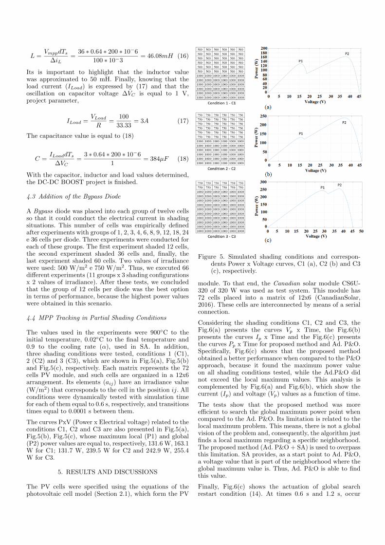
The values used in the experiments were 900C to theinitial temperature, 0.02C to the final temperature and0.9 to the cooling rate (α), used in SA. In addition,three shading conditions were tested, conditions 1 (C1),2 (C2) and 3 (C3), which are shown in Fig.5(a), Fig.5(b)and Fig.5(c), respectively. Each matrix represents the 72cells PV module, and such cells are organized in a 12x6arrangement. Its elements (aij) have an irradiance value(W/m2) that corresponds to the cell in the position ij. Allconditions were dynamically tested with simulation timefor each of them equal to 0.6 s, respectively, and transitionstimes equal to 0.0001 s between them.
The curves PxV (Power x Electrical voltage) related to theconditions C1, C2 and C3 are also presented in Fig.5(a),Fig.5(b), Fig.5(c), whose maximum local (P1) and global(P2) power values are equal to, respectively, 131.6 W, 163.1W for C1; 131.7 W, 239.5 W for C2 and 242.9 W, 255.4W for C3.
5. RESULTS AND DISCUSSIONS
The PV cells were specified using the equations of thephotovoltaic cell model (Section 2.1), which form the PV
Figure 5. Simulated shading conditions and correspon-dents Power x Voltage curves, C1 (a), C2 (b) and C3(c), respectively.
module. To that end, the Canadian solar module CS6U-320 of 320 W was used as test system. This module has72 cells placed into a matrix of 12x6 (CanadianSolar,2016). These cells are interconnected by means of a serialconnection.
Considering the shading conditions C1, C2 and C3, theFig.6(a) presents the curves Vp x Time, the Fig.6(b)presents the curves Ip x Time and the Fig.6(c) presentsthe curves Pp x Time for proposed method and Ad. P&O.Specifically, Fig.6(c) shows that the proposed methodobtained a better performance when compared to the P&Oapproach, because it found the maximum power valueon all shading conditions tested, while the Ad.P&O didnot exceed the local maximum values. This analysis iscomplemented by Fig.6(a) and Fig.6(b), which show thecurrent (Ip) and voltage (Vp) values as a function of time.
The tests show that the proposed method was moreefficient to search the global maximum power point whencompared to the Ad. P&O. Its limitation is related to thelocal maximum problem. This means, there is not a globalvision of the problem and, consequently, the algorithm justfinds a local maximum regarding a specific neighborhood.The proposed method (Ad. P&O + SA) is used to overpassthis limitation. SA provides, as a start point to Ad. P&O,a voltage value that is part of the neighborhood where theglobal maximum value is. Thus, Ad. P&O is able to findthis value.
Finally, Fig.6(c) shows the actuation of global searchrestart condition (14). At times 0.6 s and 1.2 s, occur

Figure 6. Voltage x Time (a), Current x Time (b) andPower x Time (c) resultant curves from the shadingconditions execution.
two shading conditions changes (C1-C2 and C2-C3), re-spectively. The first was detected by condition, becauseit implied a power variation higher than 10%, while thesecond is not detected. This no detection is justified by thefact that power variation, originated of shading conditionchange (C2-C3), is low enough to avoid the global searchrestart. In this case, it is likely that the Ad. P&O is able tofind the maximum power value. Thus, a more sophisticatedsearch is not necessary, as proposed by the SA.
6. CONCLUSIONS AND RESEARCH DIRECTIONS
The proposed method obtained better results when com-pared to the individual executions of the P&O approaches.
However, comparisons with other search techniques arerequired, in order to corroborate the good results obtainedwith this hybrid method. Moreover, it is intended to per-form the simulated tests on a real PV module, becausepractical results are important for the enrichment of thework developed.
Finally, an improvement to be included consists in the de-crease of the oscillations in the voltage and, consequently,in the power provided by the PV module. Abrupt changesin the reference voltage, supplied by the MPPT, causethe output voltage of the BOOST converter to oscillatemore significantly. Therefore, alternatives that minimizethe negative effects of these situations can be sought, whichis a starting point for future researches.
REFERENCES
Abdelsalam, A.K., Massoud, A.M., Ahmed, S., and Enjeti,P.N. (2011). High-performance adaptive perturb andobserve MPPT technique for photovoltaic-based micro-grids. IEEE Transactions on Power Eletronics, 26(4),1010–1021.
Ahmed, J. and Salam, Z. (2015). An improved perturband observe (P&O) maximum power point tracking(MPPT) algorithm for higher efficiency. Applied En-ergy, 150, 97–108.
Alik, R. and Jusoh, A. (2018). An enhanced P&O checkingalgorithm MPPT forhigh tracking efficiency of partiallyshaded pv module. Solar Energy, 163, 570–580.
Belhachat, F. and Larbes, C. (2018). A review of globalmaximum powerpoint tracking techniques of photo-voltaic system under partial shadingconditions. Renew-able and Sustainable Energy Reviews, 92, 513–553.
CanadianSolar (2016). MAX-POWER CS6U-315|320|325|330P.<http://download.aldo.com.br/pdfprodutos/Produto34009IdArquivo4019.pdf>. [Online] Acessadoem: 13/04/2019.
EPE (2019). Energy and electrical matrix.<http://www.epe.gov.br/pt/abcdenergia/matriz-energetica-e-eletrica>. [Online] Acessado em:02/03/2019.
Ghani, F. and Duke, M. (2011). Numerical determinationof parasitic resistances of a solar cell using the lambertw-function. Solar Energy, 85, 2386–2394.
Kobayashi, K., Matsuo, H., and Sekine, Y. (2004). A noveloptimum operating pointtracker of the solar cell powersupply system. Proceedings of the 2004 IEEE 35thannual power electronics specialists conference. PESC04, 2147–2151.
Liu, F., Kang, Y., Zhang, Y., and Duan, S. (2008). Com-parison of P&O and hillclimbing MPPT methods forgrid-connected PV converter. Proceedingsof the 3rdIEEE conference on industrial electronics and applica-tions. ICIEA 2008, IEEE, 804–807.
Rizzo, S.A. and Scelba, G. (2015). Ann based mpptmethod for rapidly variableshading conditions. ApplEnergy, 145, 124–132.
Vasarevicius, D., Martavicius, R., and Pikutis, M. (2012).Application of artificial neural networks for maximumpower point tracking of photovoltaic panels. Electronicsand Electrical Engineering, 18.