Adaptive QoS Optimizations with applications to RadarTracking ?

Sourav Ghosh1, Jeffery Hansen2, and Ragunathan (Raj) Rajkumar3 and JohnLehoczky4

1 Carnegie Mellon University, Department of Electrical and Computer Engineeringsourav@cs.cmu.edu

2 Carnegie Mellon University, Institute for Complex Engineered Systemshansen@cmu.edu3 Carnegie Mellon University, Department of Electrical and Computer Engineering

raj@ece.cmu.edu4 Carnegie Mellon University, Department of Statisticsjpl@stat.cmu.edu

Abstract. In many applications such as sensor networks, mobile ad hoc net-working and autonomous systems, the relationship between level of service andresource requirements is not fixed. Environmental factors outside the direct con-trol of the system affect this relationship and may also affect the perceived utilityof a given level of service. Radar tracking provides a good example. In radarsystems, a fixed amount of radar bandwidth and computing resources must beapportioned among multiple tasks, each of which corresponds to a target. In ad-dition, environmental factors such as noise, heating constraints of the radar andthe speed, distance and maneuverability of tracked targets dynamically affect themapping between the level of service and resource requirements as well as themapping between the level of service and the user-perceived utility. To be able tohandle these tasks, a QoS manager must be adaptive, reacting to dynamic changesin the environment, adjusting the level of service and reallocating resources effi-ciently. In this paper, we present a dynamic QoS optimization scheme for a radartracking application based on Q-RAM [1, 2]. Our scheme is able to deal with alarge number of operating points in real-time with very acceptable losses in totalutility accrued. This result is made possible by an efficient heuristic to computethe concave majorant of a multi-variate function, and an off-line storage-efficientdiscretization of the static aspects of the problem space. These two contributionswill also be useful in many dynamic QoS-driven applications beyond radar track-ing.

1 Introduction

Traditional QoS optimization algorithms assume that a collection of tasks compete forresources, with each task receiving some benefit from those resources. The goal is toallocate the resources to tasks in such a way as to optimize the total benefit received byall the tasks. This benefit is often called “utility” [3]. A larger QoS for a task generally

? This work was supported by a DARPA Multidisciplinary University Research Initiative(MURI) program administered by the Office of Naval Research under Grant N00014-01-1-0576 and by DARPA under contract number F33615-00-C-1729.

requires a larger amount of resources and results in larger utility. Furthermore, the QoS-utility curve usually saturates at a high QoS level with further increases in QoS yieldingsmaller increases in utility [1]. Generally, it is assumed that for a given invocation of atask, the utility received for a particular amount of resources is constant. While this issufficient for many applications, this may not be the case for other applications.

An example of an application where the mapping between resources and utility maychange dynamically is radar tracking. Radar tracking is challenging in that it deals witha large number of dynamic tasks, multiple resources, several practical constraints andreal-time operation. Due to the high complexity of high-quality tracking in real-time,radar systems have traditionally used rather static schemes inter-mixed with operator(somewhat error-prone) intuition of which combinations are likely to work. It is im-portant to develop real-time resource allocation algorithms that will lead near-optimalresource allocations over a wide range of conditions.

R1 only

R2 only

R3 only

R4 only

R1&R2

R2&R3 R3&R4

R1&R4

(a) Radar Layout

t

txi twi triTi

Ai

(b) Dwell Parameters

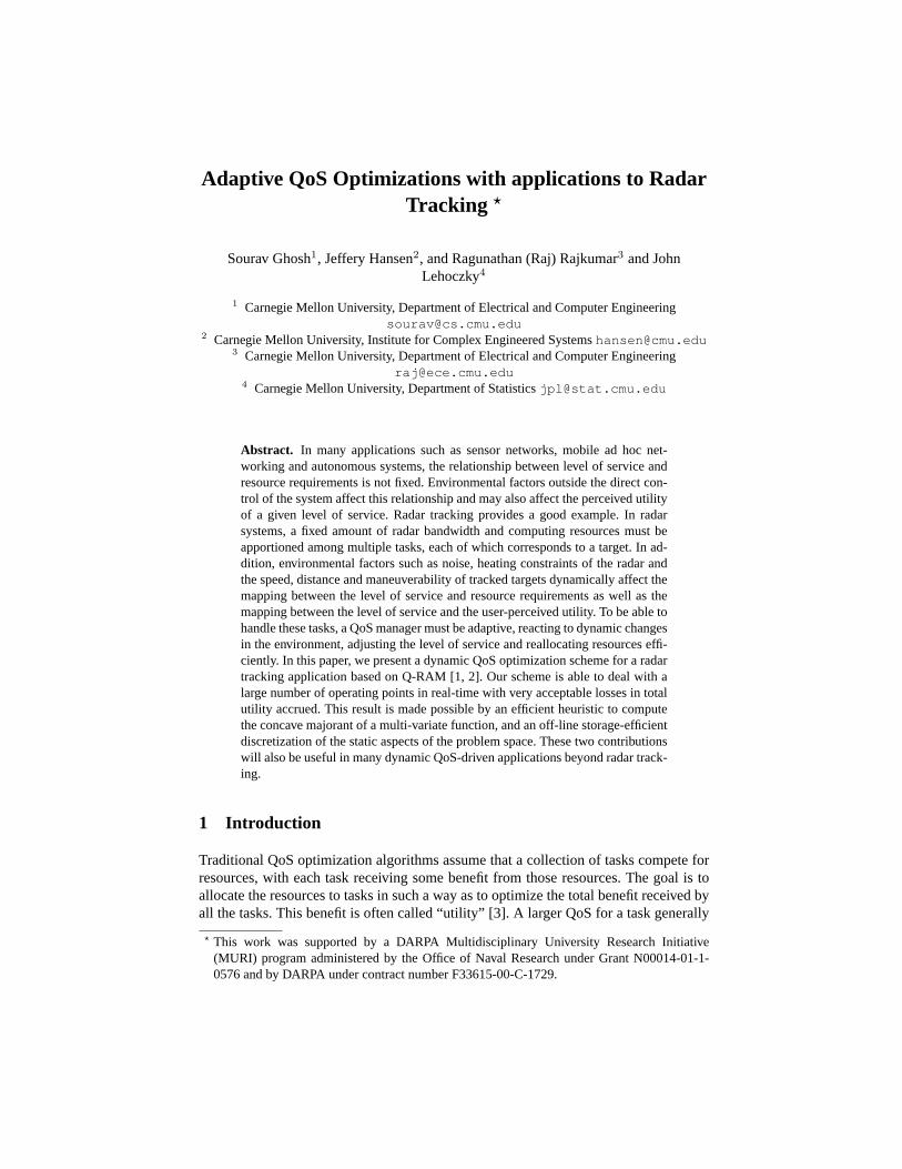
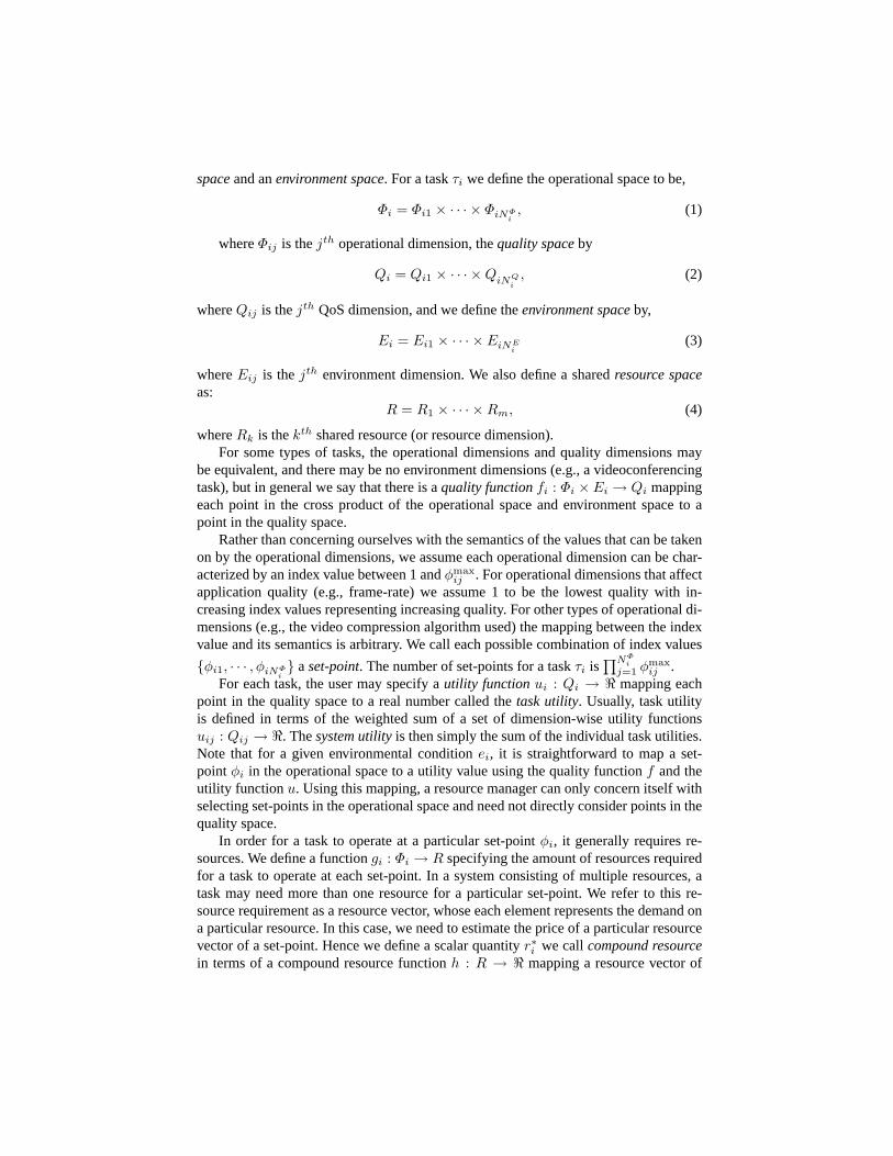
Fig. 1.Radar Model

In this paper, we model a radar system as being composed of radar transceivers,a power source and an array of processors for the signal processing and tracking algo-rithms. A radar system must also satisfy physical constraints, for example, the dynamicsof an object being tracked (such as its speed, acceleration and distance from the radar),and environmental factors such as noise influence the tracking precision. Moreover, theradar system itself imposes certain constraints. For example, not only must the utiliza-tion of the resources be below an appropriate utilization bound, other constraints suchas the heat dissipation limits of a radar transmitter must also be satisfied. The radarsystem resource management problems are as follows:

• Selection of appropriate settings or operating points for tracking tasks:Inthis paper, we address this issue. We use the QoS-based Resource Allocation Model(Q-RAM)[1, 4] as the building block of our resource management framework.

• Ensuring schedulability of the tasks:We address this in [5].Many recent studies have focused on phased-array systems, especially radar schedul-

ing. For example, Goddard et al [6] used data flow model for real-time scheduling ofradar tracking algorithms. On the other hand, Shih et al[7, 8] addressed the scheduling

issues of radar front-end. In addition, similar to our optimization methodology, theyalso introduced the idea of “service classes” designed off-line to determine the QoSoperating points of tasks.

The rest of the paper is organized as follows. Section 2 presents our model of theradar system. Section 3 presents the QoS optimization schemes in the radar system. InSection 4, we evaluate and compare these schemes. In Section 5, we quantize the prob-lem space and also perform part of the computation off-line. In Section 6, we describethe results from the quantization. Finally in Section 7, we summarize our contributionsand provide a brief description of our future work.

2 Our Radar System Model

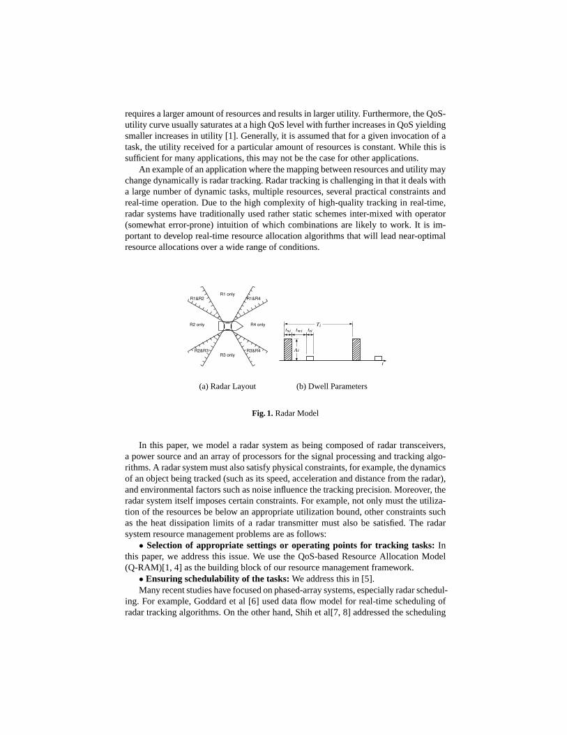
QoS and Resource Assignmentsfor tasks

QoS and Resource Specifcationsfrom Tasks

Q−RAM

Scheduler Admission Test

Request success/failure Resource reservation request to OS

Resources

CPUTime

SignalPower

Tasks

Signal

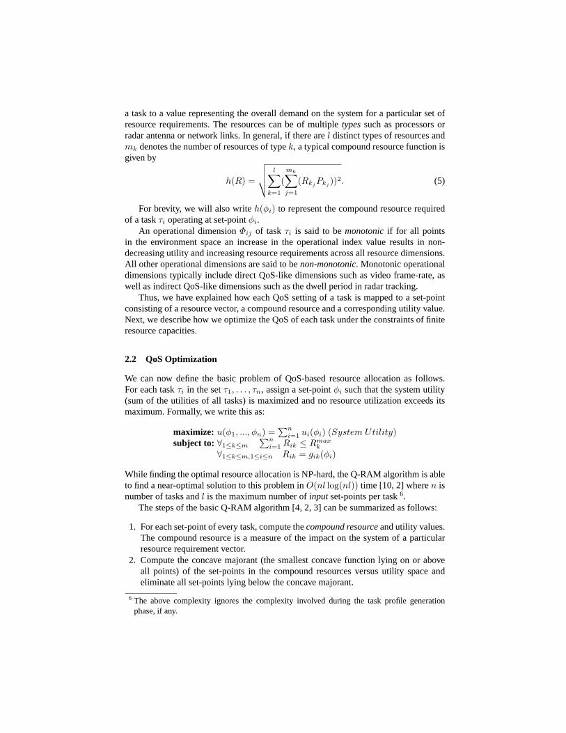
Fig. 2.Q-RAM & Scheduler Admission ControlSc

hedu

ler A

dmis

sion

Con

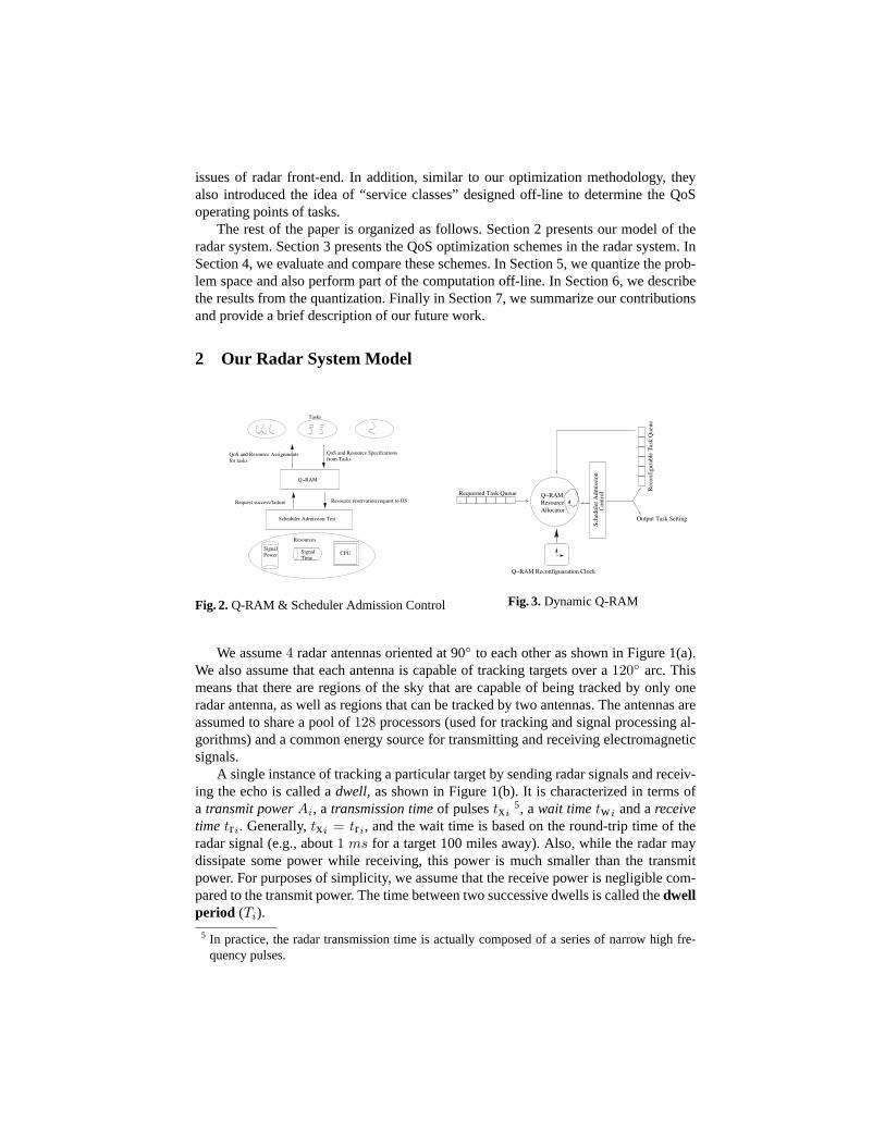
trolQ−RAM

ResourceAllocator

Requested Task Queue

Q−RAM Reconfiguaration Clock

Output Task Setting

Rec

onfi

gura

ble

Tas

k Q

ueue

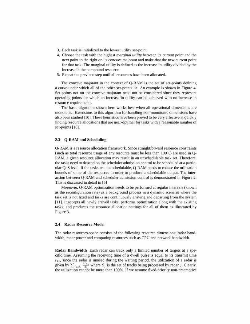
Fig. 3.Dynamic Q-RAM

We assume4 radar antennas oriented at 90◦ to each other as shown in Figure 1(a).We also assume that each antenna is capable of tracking targets over a120◦ arc. Thismeans that there are regions of the sky that are capable of being tracked by only oneradar antenna, as well as regions that can be tracked by two antennas. The antennas areassumed to share a pool of128 processors (used for tracking and signal processing al-gorithms) and a common energy source for transmitting and receiving electromagneticsignals.

A single instance of tracking a particular target by sending radar signals and receiv-ing the echo is called adwell, as shown in Figure 1(b). It is characterized in terms ofa transmit powerAi, a transmission timeof pulsestxi

5, await timetwi and areceivetime tri. Generally,txi = tri, and the wait time is based on the round-trip time of theradar signal (e.g., about1 ms for a target 100 miles away). Also, while the radar maydissipate some power while receiving, this power is much smaller than the transmitpower. For purposes of simplicity, we assume that the receive power is negligible com-pared to the transmit power. The time between two successive dwells is called thedwellperiod (Ti).

5 In practice, the radar transmission time is actually composed of a series of narrow high fre-quency pulses.

For a particular target, we obtain better tracking information by increasing the trans-mit time, reducing the dwell period,or increasing the transmission power. The powerrequirement, in turn, is inversely proportional to the fourth power of distance of thetarget from the radar as the power of the received signal at the radar is inversely of pro-portional to the fourth power of the distance [9]. Apart from the power output capabilityof the energy source, there is a limit on the amount of heat dissipation on each radartransmitter.

The tracking information is also dependent on many environmental factors beyondthe radar system’s control such as the speed, the acceleration, the distance and the typeof the target, the presence of noise in the atmosphere and the use of electronic counter-measures by the target. Several tracking algorithms are available to choose from, witheach algorithm performing better or worse with respect to computational cycles, noisetolerance, dealing with target maneuverability etc. The main tasks of an antenna are(1) Searching for targets and (2) Tracking the targets. In this paper, we only deal withtracking because search tasks can be considered to be tracking “virtual targets”. If realtargets are found by a search task, tracking tasks are initiated[5, 6, 7].

In summary, the quality of tracking a particular target depends on environmentalfactors, target dynamics as well as the usage of resources. In addition, the importanceof tracking a particular target depends on the type of the target (e.g., a friend or a foe,a helicopter or a missile), the distance of the target from the radar and the speed of thetarget towards the radar. We would like higher precision tracking for dangerous targetsthat are close to the radar, and lower precision but more resource-conserving trackingfor less dangerous ones and targets that are far away.

2.1 QoS Model

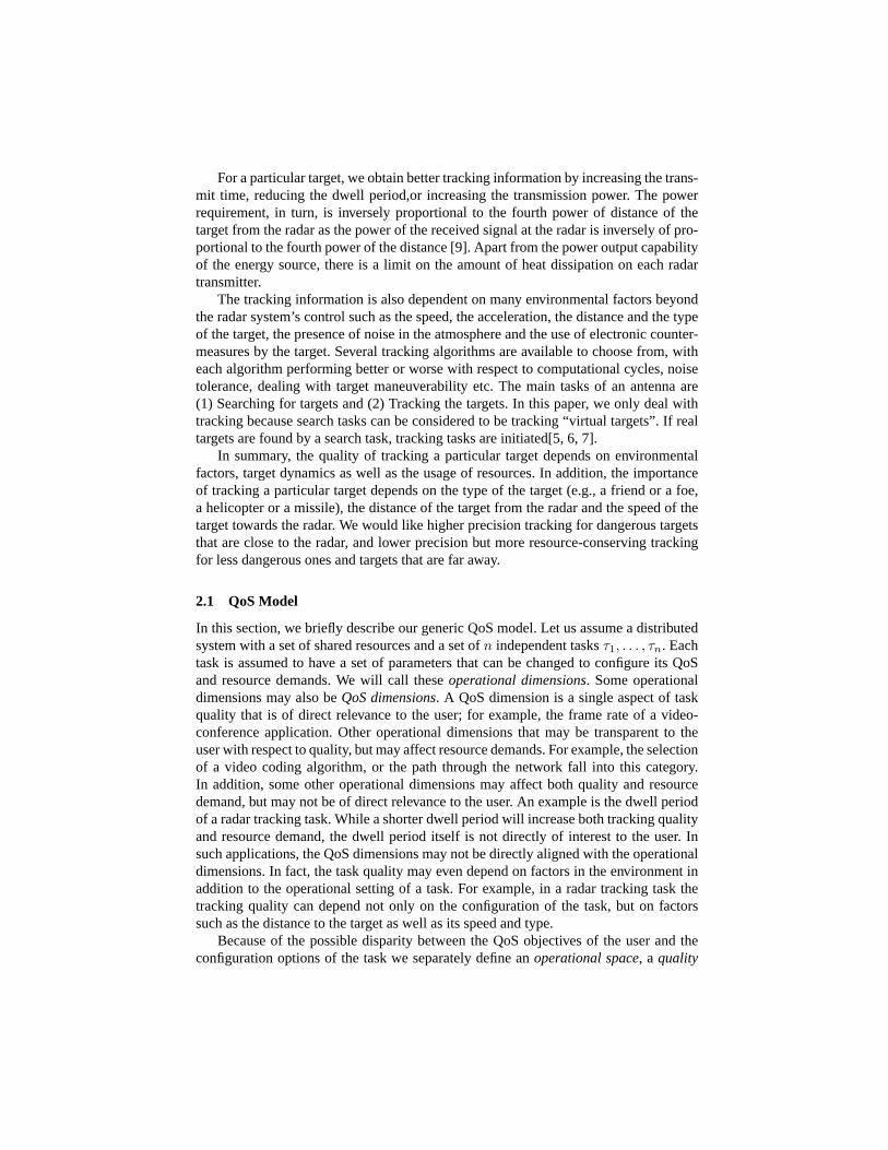
In this section, we briefly describe our generic QoS model. Let us assume a distributedsystem with a set of shared resources and a set ofn independent tasksτ1, . . . , τn. Eachtask is assumed to have a set of parameters that can be changed to configure its QoSand resource demands. We will call theseoperational dimensions. Some operationaldimensions may also beQoS dimensions. A QoS dimension is a single aspect of taskquality that is of direct relevance to the user; for example, the frame rate of a video-conference application. Other operational dimensions that may be transparent to theuser with respect to quality, but may affect resource demands. For example, the selectionof a video coding algorithm, or the path through the network fall into this category.In addition, some other operational dimensions may affect both quality and resourcedemand, but may not be of direct relevance to the user. An example is the dwell periodof a radar tracking task. While a shorter dwell period will increase both tracking qualityand resource demand, the dwell period itself is not directly of interest to the user. Insuch applications, the QoS dimensions may not be directly aligned with the operationaldimensions. In fact, the task quality may even depend on factors in the environment inaddition to the operational setting of a task. For example, in a radar tracking task thetracking quality can depend not only on the configuration of the task, but on factorssuch as the distance to the target as well as its speed and type.

Because of the possible disparity between the QoS objectives of the user and theconfiguration options of the task we separately define anoperational space, a quality

spaceand anenvironment space. For a taskτi we define the operational space to be,

Φi = Φi1 × · · · × ΦiNΦi, (1)

whereΦij is thejth operational dimension, thequality spaceby

Qi = Qi1 × · · · ×QiNQi

, (2)

whereQij is thejth QoS dimension, and we define theenvironment spaceby,

Ei = Ei1 × · · · × EiNEi

(3)

whereEij is thejth environment dimension. We also define a sharedresource spaceas:

R = R1 × · · · ×Rm, (4)

whereRk is thekth shared resource (or resource dimension).For some types of tasks, the operational dimensions and quality dimensions may

be equivalent, and there may be no environment dimensions (e.g., a videoconferencingtask), but in general we say that there is aquality functionfi : Φi ×Ei → Qi mappingeach point in the cross product of the operational space and environment space to apoint in the quality space.

Rather than concerning ourselves with the semantics of the values that can be takenon by the operational dimensions, we assume each operational dimension can be char-acterized by an index value between 1 andφmax

ij . For operational dimensions that affectapplication quality (e.g., frame-rate) we assume 1 to be the lowest quality with in-creasing index values representing increasing quality. For other types of operational di-mensions (e.g., the video compression algorithm used) the mapping between the indexvalue and its semantics is arbitrary. We call each possible combination of index values

{φi1, · · · , φiNΦi} aset-point. The number of set-points for a taskτi is

∏NΦi

j=1 φmaxij .

For each task, the user may specify autility functionui : Qi → < mapping eachpoint in the quality space to a real number called thetask utility. Usually, task utilityis defined in terms of the weighted sum of a set of dimension-wise utility functionsuij : Qij → <. Thesystem utilityis then simply the sum of the individual task utilities.Note that for a given environmental conditionei, it is straightforward to map a set-point φi in the operational space to a utility value using the quality functionf and theutility function u. Using this mapping, a resource manager can only concern itself withselecting set-points in the operational space and need not directly consider points in thequality space.

In order for a task to operate at a particular set-pointφi, it generally requires re-sources. We define a functiongi : Φi → R specifying the amount of resources requiredfor a task to operate at each set-point. In a system consisting of multiple resources, atask may need more than one resource for a particular set-point. We refer to this re-source requirement as a resource vector, whose each element represents the demand ona particular resource. In this case, we need to estimate the price of a particular resourcevector of a set-point. Hence we define a scalar quantityr∗i we callcompound resourcein terms of a compound resource functionh : R → < mapping a resource vector of

a task to a value representing the overall demand on the system for a particular set ofresource requirements. The resources can be of multipletypessuch as processors orradar antenna or network links. In general, if there arel distinct types of resources andmk denotes the number of resources of typek, a typical compound resource function isgiven by

h(R) =

√√√√ l∑k=1

(mk∑j=1

(RkjPkj

))2. (5)

For brevity, we will also writeh(φi) to represent the compound resource requiredof a taskτi operating at set-pointφi.

An operational dimensionΦij of taskτi is said to bemonotonicif for all pointsin the environment space an increase in the operational index value results in non-decreasing utility and increasing resource requirements across all resource dimensions.All other operational dimensions are said to benon-monotonic. Monotonic operationaldimensions typically include direct QoS-like dimensions such as video frame-rate, aswell as indirect QoS-like dimensions such as the dwell period in radar tracking.

Thus, we have explained how each QoS setting of a task is mapped to a set-pointconsisting of a resource vector, a compound resource and a corresponding utility value.Next, we describe how we optimize the QoS of each task under the constraints of finiteresource capacities.

2.2 QoS Optimization

We can now define the basic problem of QoS-based resource allocation as follows.For each taskτi in the setτ1, . . . , τn, assign a set-pointφi such that the system utility(sum of the utilities of all tasks) is maximized and no resource utilization exceeds itsmaximum. Formally, we write this as:

maximize: u(φ1, ..., φn) =∑n

i=1 ui(φi) (System Utility)subject to: ∀1≤k≤m

∑ni=1 Rik ≤ Rmax

k

∀1≤k≤m,1≤i≤n Rik = gik(φi)

While finding the optimal resource allocation is NP-hard, the Q-RAM algorithm is ableto find a near-optimal solution to this problem inO(nl log(nl)) time [10, 2] wheren isnumber of tasks andl is the maximum number ofinputset-points per task6.

The steps of the basic Q-RAM algorithm [4, 2, 3] can be summarized as follows:

1. For each set-point of every task, compute thecompound resourceand utility values.The compound resource is a measure of the impact on the system of a particularresource requirement vector.

2. Compute the concave majorant (the smallest concave function lying on or aboveall points) of the set-points in the compound resources versus utility space andeliminate all set-points lying below the concave majorant.

6 The above complexity ignores the complexity involved during the task profile generationphase, if any.

3. Each task is initialized to the lowest utility set-point.4. Choose the task with the highestmarginal utility between its current point and the

next point to the right on its concave majorant and make that the new current pointfor that task. The marginal utility is defined as the increase in utility divided by theincrease in the compound resource.

5. Repeat the previous step until all resources have been allocated.

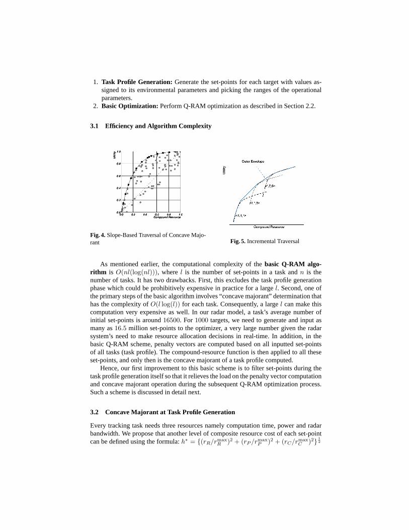
The concave majorant in the context of Q-RAM is the set of set-points defininga curve under which all of the other set-points lie. An example is shown in Figure 4.Set-points not on the concave majorant need not be considered since they representoperating points for which an increase in utility can be achieved with no increase inresource requirements.

The basic algorithm shown here works best when all operational dimensions aremonotonic. Extensions to this algorithm for handling non-monotonic dimensions havealso been studied [10]. These heuristics have been proved to be very effective at quicklyfinding resource allocations that are near-optimal for tasks with a reasonable number ofset-points [10].

2.3 Q-RAM and Scheduling

Q-RAM is a resource allocation framework. Since straightforward resource constraints(such as total resource usage of any resource must be less than 100%) are used in Q-RAM, a given resource allocation may result in an unschedulable task set. Therefore,the tasks need to depend on the scheduler admission control to be scheduled at a partic-ular QoS level. If the tasks are not schedulable, Q-RAM needs to reduce the utilizationbounds of some of the resources in order to produce a schedulable output. The inter-action between Q-RAM and scheduler admission control is demonstrated in Figure 2.This is discussed in detail in [5]

Moreover, Q-RAM optimization needs to be performed at regular intervals (knownas the reconfiguration rate) as a background process in a dynamic scenario where thetask set is not fixed and tasks are continuously arriving and departing from the system[11]. It accepts all newly arrived tasks, performs optimization along with the existingtasks, and produces the resource allocation settings for all of them as illustrated byFigure 3.

2.4 Radar Resource Model

The radar resources-space consists of the following resource dimensions: radar band-width, radar power and computing resources such as CPU and network bandwidth.

Radar Bandwidth Each radar can track only a limited number of targets at a spe-cific time. Assuming the receiving time of a dwell pulse is equal to its transmit timetxi, since the radar is unused during the waiting period, the utilization of a radar isgiven by

∑i∈Sj

2txi

TiwhereSj is the set of tracks being processed by radarj. Clearly,

the utilization cannot be more than 100%. If we assume fixed-priority non-preemptive

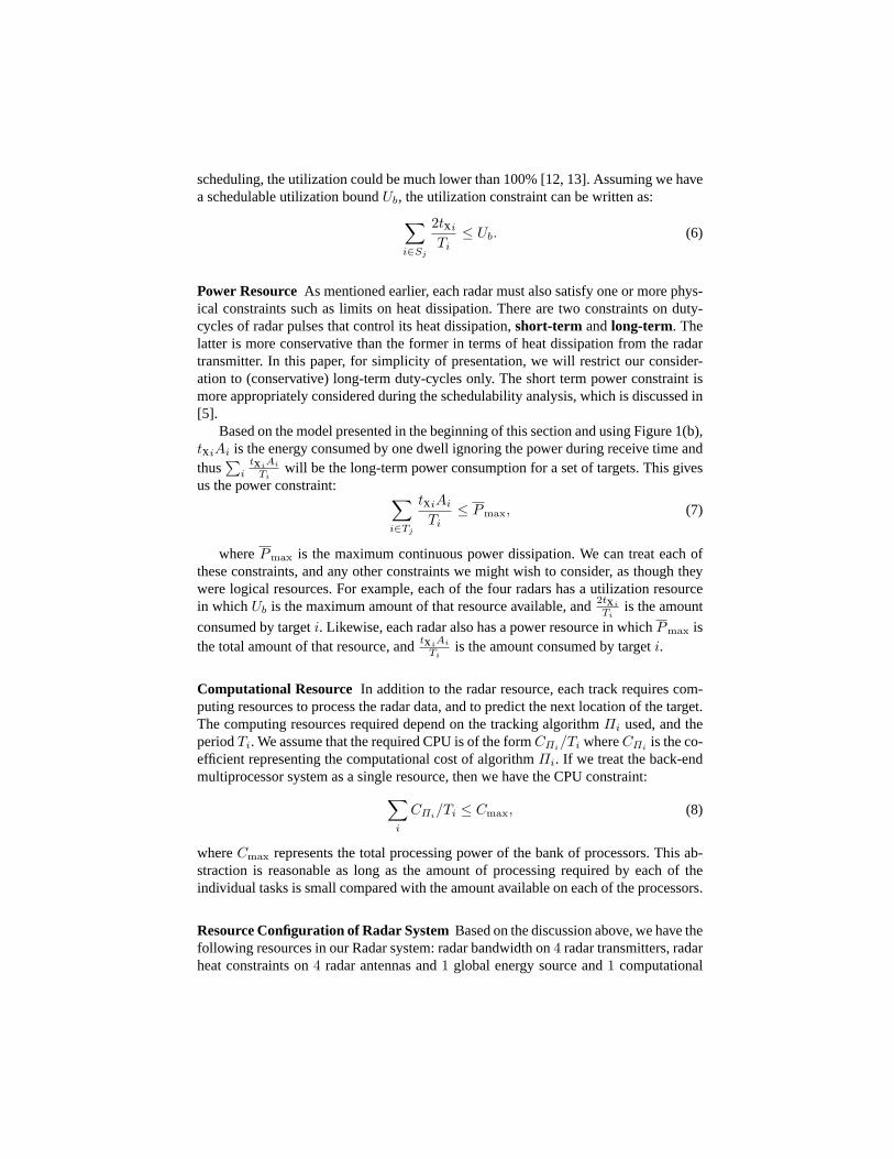
scheduling, the utilization could be much lower than 100% [12, 13]. Assuming we havea schedulable utilization boundUb, the utilization constraint can be written as:∑

i∈Sj

2txi

Ti≤ Ub. (6)

Power ResourceAs mentioned earlier, each radar must also satisfy one or more phys-ical constraints such as limits on heat dissipation. There are two constraints on duty-cycles of radar pulses that control its heat dissipation,short-term andlong-term. Thelatter is more conservative than the former in terms of heat dissipation from the radartransmitter. In this paper, for simplicity of presentation, we will restrict our consider-ation to (conservative) long-term duty-cycles only. The short term power constraint ismore appropriately considered during the schedulability analysis, which is discussed in[5].

Based on the model presented in the beginning of this section and using Figure 1(b),txiAi is the energy consumed by one dwell ignoring the power during receive time andthus

∑i

txiAi

Tiwill be the long-term power consumption for a set of targets. This gives

us the power constraint: ∑i∈Tj

txiAi

Ti≤ Pmax, (7)

wherePmax is the maximum continuous power dissipation. We can treat each ofthese constraints, and any other constraints we might wish to consider, as though theywere logical resources. For example, each of the four radars has a utilization resourcein whichUb is the maximum amount of that resource available, and2txi

Tiis the amount

consumed by targeti. Likewise, each radar also has a power resource in whichPmax isthe total amount of that resource, andtxiAi

Tiis the amount consumed by targeti.

Computational Resource In addition to the radar resource, each track requires com-puting resources to process the radar data, and to predict the next location of the target.The computing resources required depend on the tracking algorithmΠi used, and theperiodTi. We assume that the required CPU is of the formCΠi/Ti whereCΠi is the co-efficient representing the computational cost of algorithmΠi. If we treat the back-endmultiprocessor system as a single resource, then we have the CPU constraint:∑

i

CΠi/Ti ≤ Cmax, (8)

whereCmax represents the total processing power of the bank of processors. This ab-straction is reasonable as long as the amount of processing required by each of theindividual tasks is small compared with the amount available on each of the processors.

Resource Configuration of Radar SystemBased on the discussion above, we have thefollowing resources in our Radar system: radar bandwidth on4 radar transmitters, radarheat constraints on4 radar antennas and1 global energy source and1 computational

resource from the ship. Therefore, our resource vector consists of10 components. Theglobal computational processor allocation has been studied in [10], and we treat it as asingle resource.

2.5 Tracking QoS Model

There are two principal QoS dimensions in the quality space of the radar tracking prob-lem:

• Tracking error: This is the difference between the actual position and the trackedposition of the target. Although one cannot know the true tracking error, many track-ing algorithms yield estimates and their precision of a particular tracking result. Asmentioned in Section 2.4, this tracking precision is dependent on the availability ofthe physical resources in addition to the computing resources. A smaller tracking errorleads to better tracking precision and hence better quality of tracking. Therefore, weassume that the tracking qualityqtrack is inversely related to the tracking errorε.

• Reliability: This is the probability that there are no hardware/software failures ina specified time interval. Higher reliability of a task is obtained by the replicated use ofresources, such as using two radars to track a single target.

In this paper, we focus only on tracking error, and refer the reader to [10] for a studyof how the number of replicas for a particular computation is integrated into Q-RAM.

Next, we list the operational and environmental dimensions of the system.

Operational Dimensions In our tracking model, the operational dimensions are dwellperiod (Ti), dwell time (txi), dwell power (Ai), and choice of the tracking algorithmΠi.

The above parameters can be controlled by the system designer or the optimizer inorder to achieve the desired quality of tracking of a target.

Environmental dimensions The environmental dimensions we consider are thetypeof targetξi (e.g., airplane, helicopter, missile etc.), the distance of the target from theradarri, the velocity vector of the targetvi, the acceleration vector of the targetai, theactive noise or the presence of electro-magnetic interference such as counter-measuresni, and the angular location of the target in the sky.

Considering all the operational and environmental dimensions, we can write a func-tion,

εi = E(ξi, ri,vi,ai, ni︸ ︷︷ ︸environmental

, Ti, txi, Ai,Πi︸ ︷︷ ︸operational

), (9)

that estimates the tracking errorεi as a function of the position of the target along theenvironmental and operational dimensions. Higher tracking quality yields higher utility.For the purposes of this paper, we assume that the utility of tracking a target for a certainquality qtrack is given by the following concave exponential function,

U(qtrack) = w(1− e−βqtrack), (10)

whereβ is a parameter specific to the ranges of the speeds of three different typesof targets (airplane, missile or helicopter). It assumes the utility increases with increase

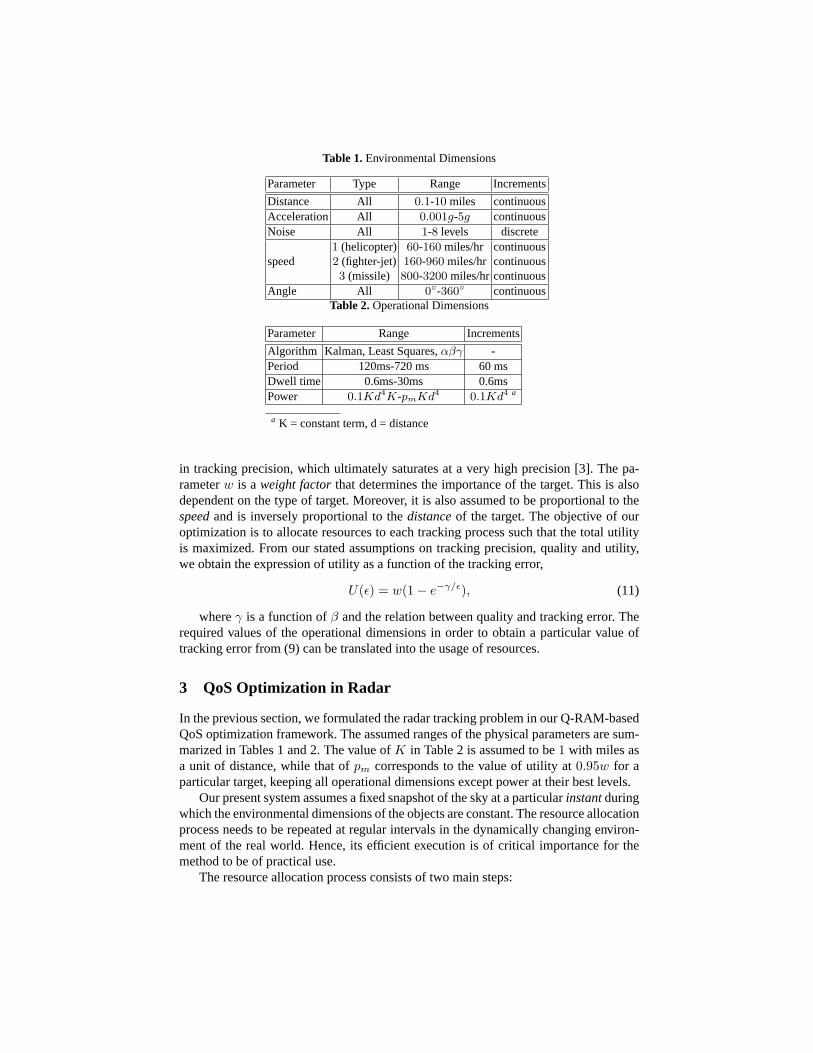
Table 1.Environmental Dimensions

Parameter Type Range Increments

Distance All 0.1-10 miles continuousAcceleration All 0.001g-5g continuousNoise All 1-8 levels discrete

1 (helicopter) 60-160 miles/hr continuousspeed 2 (fighter-jet) 160-960 miles/hr continuous

3 (missile) 800-3200 miles/hrcontinuousAngle All 0◦-360◦ continuous

Table 2.Operational Dimensions

Parameter Range Increments

Algorithm Kalman, Least Squares,αβγ -Period 120ms-720 ms 60 msDwell time 0.6ms-30ms 0.6msPower 0.1Kd4K-pmKd4 0.1Kd4 a

a K = constant term, d = distance

in tracking precision, which ultimately saturates at a very high precision [3]. The pa-rameterw is aweight factorthat determines the importance of the target. This is alsodependent on the type of target. Moreover, it is also assumed to be proportional to thespeedand is inversely proportional to thedistanceof the target. The objective of ouroptimization is to allocate resources to each tracking process such that the total utilityis maximized. From our stated assumptions on tracking precision, quality and utility,we obtain the expression of utility as a function of the tracking error,

U(ε) = w(1− e−γ/ε), (11)

whereγ is a function ofβ and the relation between quality and tracking error. Therequired values of the operational dimensions in order to obtain a particular value oftracking error from (9) can be translated into the usage of resources.

3 QoS Optimization in Radar

In the previous section, we formulated the radar tracking problem in our Q-RAM-basedQoS optimization framework. The assumed ranges of the physical parameters are sum-marized in Tables 1 and 2. The value ofK in Table 2 is assumed to be1 with miles asa unit of distance, while that ofpm corresponds to the value of utility at0.95w for aparticular target, keeping all operational dimensions except power at their best levels.

Our present system assumes a fixed snapshot of the sky at a particularinstantduringwhich the environmental dimensions of the objects are constant. The resource allocationprocess needs to be repeated at regular intervals in the dynamically changing environ-ment of the real world. Hence, its efficient execution is of critical importance for themethod to be of practical use.

The resource allocation process consists of two main steps:

1. Task Profile Generation: Generate the set-points for each target with values as-signed to its environmental parameters and picking the ranges of the operationalparameters.

2. Basic Optimization: Perform Q-RAM optimization as described in Section 2.2.

3.1 Efficiency and Algorithm Complexity

Fig. 4.Slope-Based Traversal of Concave Majo-rant Fig. 5. Incremental Traversal

As mentioned earlier, the computational complexity of thebasic Q-RAM algo-rithm is O(nl(log(nl))), wherel is the number of set-points in a task andn is thenumber of tasks. It has two drawbacks. First, this excludes the task profile generationphase which could be prohibitively expensive in practice for a largel. Second, one ofthe primary steps of the basic algorithm involves “concave majorant” determination thathas the complexity ofO(l log(l)) for each task. Consequently, a largel can make thiscomputation very expensive as well. In our radar model, a task’s average number ofinitial set-points is around16500. For 1000 targets, we need to generate and input asmany as16.5 million set-points to the optimizer, a very large number given the radarsystem’s need to make resource allocation decisions in real-time. In addition, in thebasic Q-RAM scheme, penalty vectors are computed based on all inputted set-pointsof all tasks (task profile). The compound-resource function is then applied to all theseset-points, and only then is the concave majorant of a task profile computed.

Hence, our first improvement to this basic scheme is to filter set-points during thetask profile generation itself so that it relieves the load on the penalty vector computationand concave majorant operation during the subsequent Q-RAM optimization process.Such a scheme is discussed in detail next.

3.2 Concave Majorant at Task Profile Generation

Every tracking task needs three resources namely computation time, power and radarbandwidth. We propose that another level of composite resource cost of each set-pointcan be defined using the formula:h∗ = {(rR/rmax

R )2 + (rP /rmaxP )2 + (rC/rmax

C )2} 12

during task profile generation process. The parametersrR, rP and rC are the totalamount of radar bandwidth, power and computational resource required by each taskfor its a given set-point irrespective of the particular radar and CPU to which it couldbe mapped.rmax

R , rmaxP andrmax

C are the total resource capacities for radar, power andCPU. Unlike the compound resource evaluation during the Q-RAM optimization pro-cess, this pre-processed compound resource does not require us to evaluate the penaltyvector-based demand of resources which considers all set-points of all the tasks to-gether. Next, we immediately perform the concave majorant operation on these set-points during the task profile generation. We refer to this scheme asConcave MajorantOnly in subsequent discussions, and it leads to significant load reduction in the con-cave majorant operation of the optimization step that requires us to evaluate the penaltyvector of resources.

3.3 Concave-Majorant Approximation

The complexity of computing the concave majorant can be further improved. We presentseveral pre-processing heuristics that can be performed prior to actually computing theconcave majorant. For the sake of illustration, we will first assume that all tasks haveonly monotonic operational dimensions. Later, we shall consider the case of havingsome operational dimensions that are non-monotonic.

Slope-based Traversal (ST)Let the minimumset-point for a taskτi for which alloperational dimensions are monotonic be defined asomin

i = {1, . . . , 1}, and let themaximumset-point be defined asomax

i = {vmaxi1 , . . . , vmax

iNΦi

}. Clearly, all of the set-

points in the utility/compound resource space that lie below a “terminating” line from(u(vmin

i ), h(vmini )) to (u(vmax

i ), h(vmaxi )) as shown in Figure 4 cannot be on the con-

cave majorant. These points can be eliminated immediately without being passed on tothe concave majorant step. We call this heuristic “slope-based traversal” (ST). Whilethis heuristic can reduce the time to compute the concave majorant by a constant fac-tor, it must still scan all of the set-points to determine if they are above or below theterminating line.

Fast Set-point TraversalsWe now consider a set of fast traversal heuristics that do notrequire computations for all of the set-points. We (temporarily) assume that all opera-tional dimensions are monotonic. A key observation we made is that when the actualconcave majorant is generated using all of the set-points for typical tasks, the concavemajorant tends to consists of runs of set-points which vary in onlyonedimension at atime with occasional jumps between runs of points. This insight suggests that we canuse local search techniques to follow the set-points up the concave majorant. We alsoknow thatomin

i will always be the first point on the concave majorant andomaxi will

always be the last. The different methods presented here differ primarily in the methodused to perform the local search. As an example, consider a task with three operationaldimensions. If we consider the subset of the set-points< 1, 1, ∗ > consisting of all theset-points for which dimensions 1 and 2 have index value 1, these points will tend to

1 2 3 4 5 6101

102

103

104

105

Traversal AlgorithmsN

umbe

r of

Set

−po

ints

/Tas

k (lo

gsca

le)

1.Basic Q−RAM2. Concave−Majorant3. ST4. FOFT5. 2−FOFT6. SOFT

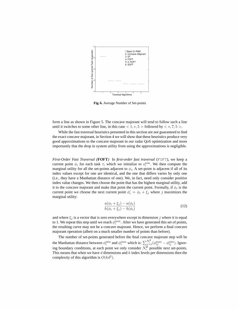
Fig. 6.Average Number of Set-points

form a line as shown in Figure 5. The concave majorant will tend to follow such a lineuntil it switches to some other line, in this case< 1, ∗, 5 > followed by< ∗, 7, 5 >.

While the fast traversal heuristics presented in this section are not guaranteed to findthe exact concave majorant, in Section 4 we will show that these heuristics produce verygood approximations to the concave majorant in our radar QoS optimization and moreimportantly that the drop in system utility from using the approximations is negligible.

First-Order Fast Traversal (FOFT) In first-order fast traversal(FOFT), we keep acurrent pointφi for each taskτi which we initialize toomin

i . We then compute themarginal utility for all the set-points adjacent toφi. A set-point is adjacent if all of itsindex values except for one are identical, and the one that differs varies by only one(i.e., they have a Manhattan distance of one). We, in fact, need only consider positiveindex value changes. We then choose the point that has the highest marginal utility, addit to the concave majorant and make that point the current point. Formally, ifφi is thecurrent point we choose the next current pointφ′i = φi + ξj wherej maximizes themarginal utility:

u(φi + ξj)− u(φi)h(φi + ξj)− h(φi)

(12)

and whereξj is a vector that is zero everywhere except in dimensionj where it is equalto 1. We repeat this step until we reachφmax

i . After we have generated this set of points,the resulting curve may not be a concave majorant. Hence, we perform a final concavemajorant operation (albeit on a much smaller number of points than before).

The number of set-points generated before the final concave majorant step will be

the Manhattan distance betweenφmini andφmax

i which is:∑NΦ

ij=1(φ

maxij − φmin

ij ). Ignor-ing boundary conditions, at each point we only considerNΦ

i possible next set-points.This means that when we haved dimensions andk index levels per dimensions then thecomplexity of this algorithm isO(kd2).

0.01

0.1

1

10

100

1000

0 100 200 300 400 500 600

Exe

cutio

n Ti

me

(s) i

n lo

gsca

le ->

Number of Tasks->

With Basic Q-RAMConcave Majorant Only

STFOFT

2-FOFTSOFT

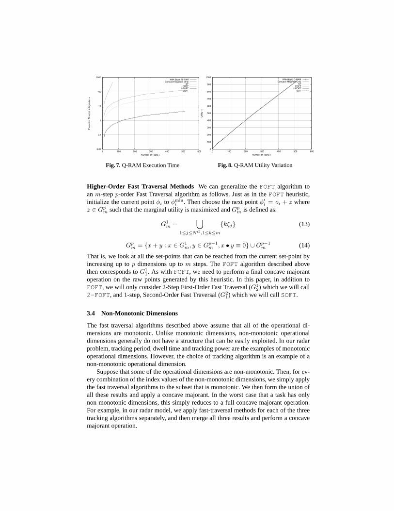
Fig. 7.Q-RAM Execution Time

0

100

200

300

400

500

600

700

800

900

1000

0 100 200 300 400 500 600

Util

ity ->

Number of Tasks->

With Basic Q-RAMConcave Majorant Only

STFOFT

2-FOFTSOT

Fig. 8.Q-RAM Utility Variation

Higher-Order Fast Traversal Methods We can generalize theFOFT algorithm toan m-stepp-order Fast Traversal algorithm as follows. Just as in theFOFTheuristic,initialize the current pointφi to φmin

i . Then choose the next pointφ′i = oi + z wherez ∈ Gp

m such that the marginal utility is maximized andGpm is defined as:

G1m =

⋃1≤j≤NO,1≤k≤m

{kξj} (13)

Gpm = {x + y : x ∈ G1

m, y ∈ Gp−1m , x • y ≡ 0} ∪Gp−1

m (14)

That is, we look at all the set-points that can be reached from the current set-point byincreasing up top dimensions up tom steps. TheFOFT algorithm described abovethen corresponds toG1

1. As with FOFT, we need to perform a final concave majorantoperation on the raw points generated by this heuristic. In this paper, in addition toFOFT, we will only consider 2-Step First-Order Fast Traversal (G1

2) which we will call2-FOFT , and 1-step, Second-Order Fast Traversal (G2

1) which we will callSOFT.

3.4 Non-Monotonic Dimensions

The fast traversal algorithms described above assume that all of the operational di-mensions are monotonic. Unlike monotonic dimensions, non-monotonic operationaldimensions generally do not have a structure that can be easily exploited. In our radarproblem, tracking period, dwell time and tracking power are the examples of monotonicoperational dimensions. However, the choice of tracking algorithm is an example of anon-monotonic operational dimension.

Suppose that some of the operational dimensions are non-monotonic. Then, for ev-ery combination of the index values of the non-monotonic dimensions, we simply applythe fast traversal algorithms to the subset that is monotonic. We then form the union ofall these results and apply a concave majorant. In the worst case that a task has onlynon-monotonic dimensions, this simply reduces to a full concave majorant operation.For example, in our radar model, we apply fast-traversal methods for each of the threetracking algorithms separately, and then merge all three results and perform a concavemajorant operation.

Conc−Majorant ST FOFT 2−FOFT SOT0

10

20

30

40

50

60

70

80

90

100

Traversal Algorithms

Per

cent

age

Exe

cutio

n Ti

me

(a) Profile Generation Time (%)

ST FOFT 2−FOFT SOFT

0

1

2

3

4

5

6

7

8

9

10

Traversal Algorithms

Per

cent

age

Loss

in U

tility

(b) Utility loss (%)

Conc−Majorant ST FOFT 2−FOFT SOT0

10

20

30

40

50

60

70

80

90

100

Traversal Algorithms

Per

cent

age

Exe

cutio

n Ti

me

(c) Optimization Time (%)

Conv−Majorant ST FOFT 2−FOFT SOFT0

10

20

30

40

50

60

70

80

90

100

Traversal Algorithms

Per

cent

age

Pro

file

Run

−Tim

e

(d) Fractional Profile Time (%)

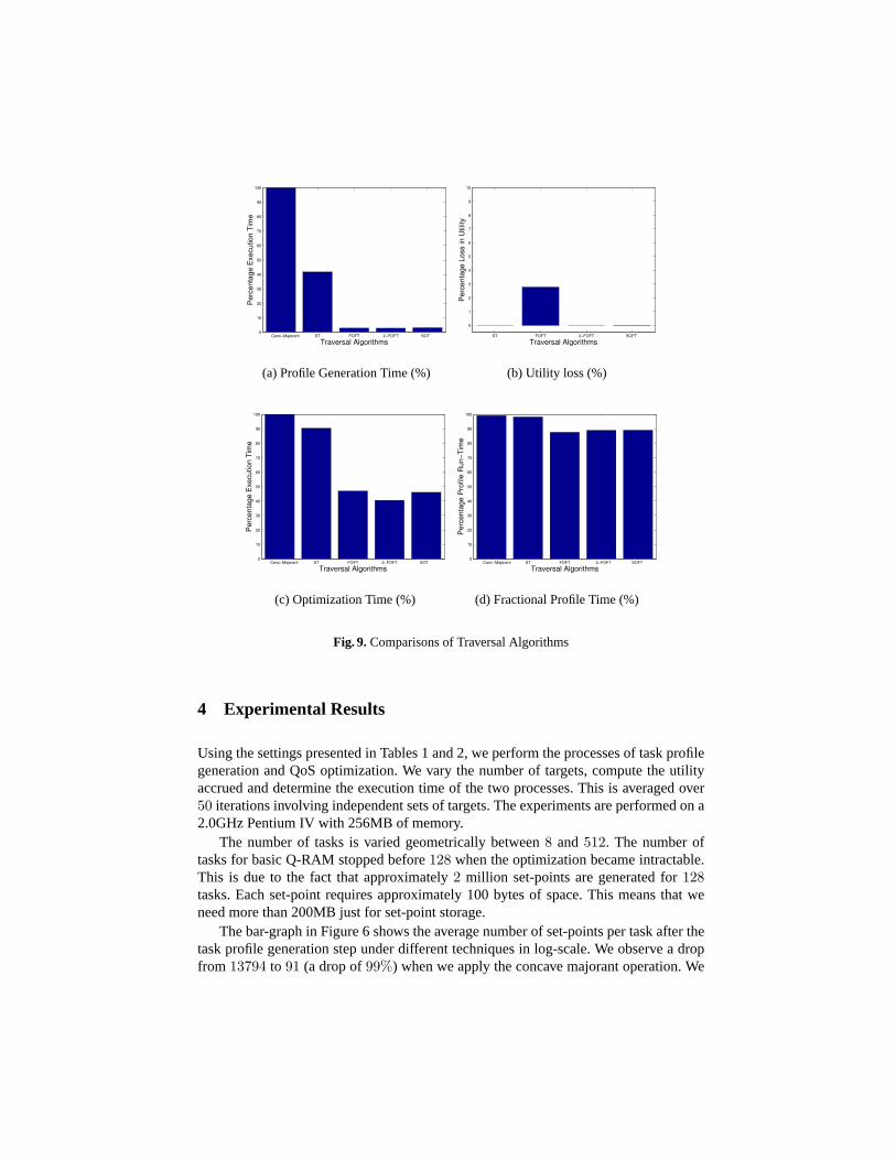
Fig. 9.Comparisons of Traversal Algorithms

4 Experimental Results

Using the settings presented in Tables 1 and 2, we perform the processes of task profilegeneration and QoS optimization. We vary the number of targets, compute the utilityaccrued and determine the execution time of the two processes. This is averaged over50 iterations involving independent sets of targets. The experiments are performed on a2.0GHz Pentium IV with 256MB of memory.

The number of tasks is varied geometrically between8 and512. The number oftasks for basic Q-RAM stopped before128 when the optimization became intractable.This is due to the fact that approximately2 million set-points are generated for128tasks. Each set-point requires approximately 100 bytes of space. This means that weneed more than 200MB just for set-point storage.

The bar-graph in Figure 6 shows the average number of set-points per task after thetask profile generation step under different techniques in log-scale. We observe a dropfrom 13794 to 91 (a drop of99%) when we apply the concave majorant operation. We

also observe that2-FOFT reduces the number of points further to47, which is a48%drop compared to the full concave majorant scheme.

0

1

2

3

4

5

6

7

8

9

10

11

0 1 2 3 4 5 6 7 8 9 10

Util

ty ->

Distance ->

Distance Variation

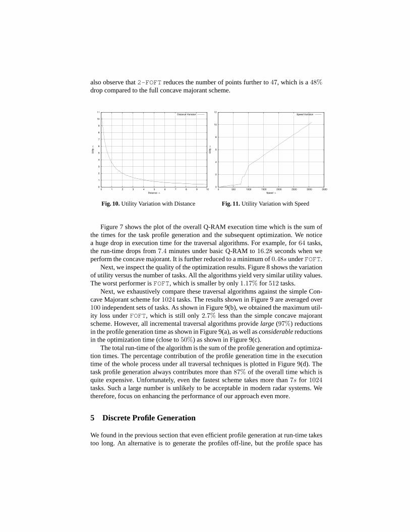
Fig. 10.Utility Variation with Distance

0

2

4

6

8

10

12

0 500 1000 1500 2000 2500 3000 3500

Util

ty ->

Speed ->

Speed Variation

Fig. 11.Utility Variation with Speed

Figure 7 shows the plot of the overall Q-RAM execution time which is the sum ofthe times for the task profile generation and the subsequent optimization. We noticea huge drop in execution time for the traversal algorithms. For example, for64 tasks,the run-time drops from7.4 minutes under basic Q-RAM to16.28 seconds when weperform the concave majorant. It is further reduced to a minimum of0.48s underFOFT.

Next, we inspect the quality of the optimization results. Figure 8 shows the variationof utility versus the number of tasks. All the algorithms yield very similar utility values.The worst performer isFOFT, which is smaller by only1.17% for 512 tasks.

Next, we exhaustively compare these traversal algorithms against the simple Con-cave Majorant scheme for1024 tasks. The results shown in Figure 9 are averaged over100 independent sets of tasks. As shown in Figure 9(b), we obtained the maximum util-ity loss underFOFT, which is still only2.7% less than the simple concave majorantscheme. However, all incremental traversal algorithms providelarge (97%) reductionsin the profile generation time as shown in Figure 9(a), as well asconsiderablereductionsin the optimization time (close to50%) as shown in Figure 9(c).

The total run-time of the algorithm is the sum of the profile generation and optimiza-tion times. The percentage contribution of the profile generation time in the executiontime of the whole process under all traversal techniques is plotted in Figure 9(d). Thetask profile generation always contributes more than87% of the overall time which isquite expensive. Unfortunately, even the fastest scheme takes more than7s for 1024tasks. Such a large number is unlikely to be acceptable in modern radar systems. Wetherefore, focus on enhancing the performance of our approach even more.

5 Discrete Profile Generation

We found in the previous section that even efficient profile generation at run-time takestoo long. An alternative is to generate the profiles off-line, but the profile space has

1.38

1.4

1.42

1.44

1.46

1.48

1.5

1.52

1.54

1.56

0 20 40 60 80 100 120 140 160

Util

ity->

Acceleration->

Acceleration Variation

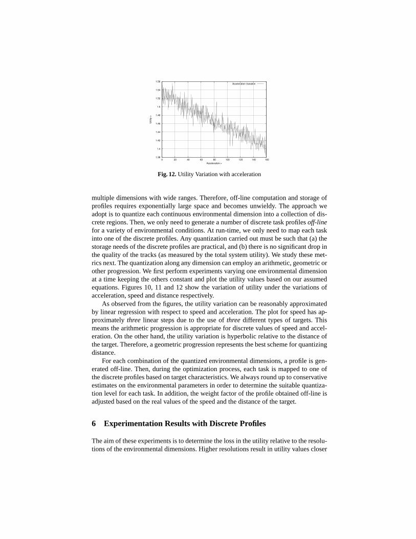
Fig. 12.Utility Variation with acceleration

multiple dimensions with wide ranges. Therefore, off-line computation and storage ofprofiles requires exponentially large space and becomes unwieldy. The approach weadopt is to quantize each continuous environmental dimension into a collection of dis-crete regions. Then, we only need to generate a number of discrete task profilesoff-linefor a variety of environmental conditions. At run-time, we only need to map each taskinto one of the discrete profiles. Any quantization carried out must be such that (a) thestorage needs of the discrete profiles are practical, and (b) there is no significant drop inthe quality of the tracks (as measured by the total system utility). We study these met-rics next. The quantization along any dimension can employ an arithmetic, geometric orother progression. We first perform experiments varying one environmental dimensionat a time keeping the others constant and plot the utility values based on our assumedequations. Figures 10, 11 and 12 show the variation of utility under the variations ofacceleration, speed and distance respectively.

As observed from the figures, the utility variation can be reasonably approximatedby linear regression with respect to speed and acceleration. The plot for speed has ap-proximatelythree linear steps due to the use ofthreedifferent types of targets. Thismeans the arithmetic progression is appropriate for discrete values of speed and accel-eration. On the other hand, the utility variation is hyperbolic relative to the distance ofthe target. Therefore, a geometric progression represents the best scheme for quantizingdistance.

For each combination of the quantized environmental dimensions, a profile is gen-erated off-line. Then, during the optimization process, each task is mapped to one ofthe discrete profiles based on target characteristics. We always round up to conservativeestimates on the environmental parameters in order to determine the suitable quantiza-tion level for each task. In addition, the weight factor of the profile obtained off-line isadjusted based on the real values of the speed and the distance of the target.

6 Experimentation Results with Discrete Profiles

The aim of these experiments is to determine the loss in the utility relative to the resolu-tions of the environmental dimensions. Higher resolutions result in utility values closer

to the optimal, but require more storage for off-line profiling. Also, one dimension maybe more dominant in influencing the utility value than others, hence we need higherresolution for this dimension. Thus, we have a trade-off between the loss in utility andstorage space.

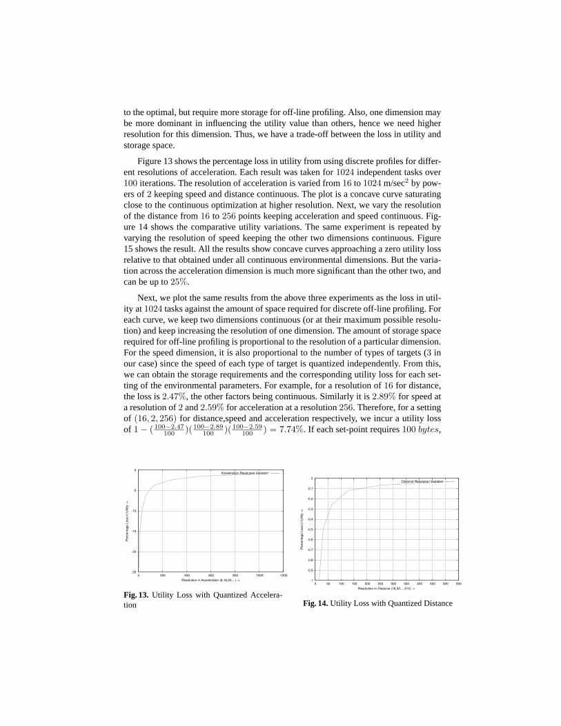
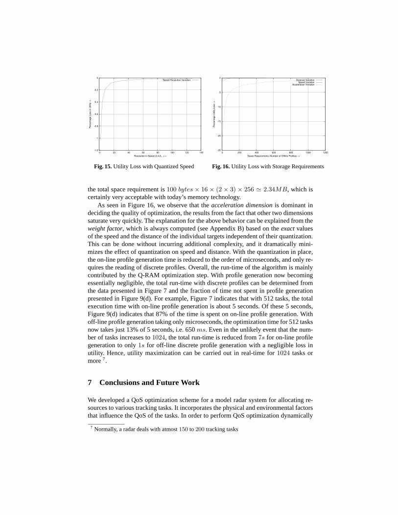
Figure 13 shows the percentage loss in utility from using discrete profiles for differ-ent resolutions of acceleration. Each result was taken for1024 independent tasks over100 iterations. The resolution of acceleration is varied from16 to 1024 m/sec2 by pow-ers of2 keeping speed and distance continuous. The plot is a concave curve saturatingclose to the continuous optimization at higher resolution. Next, we vary the resolutionof the distance from16 to 256 points keeping acceleration and speed continuous. Fig-ure 14 shows the comparative utility variations. The same experiment is repeated byvarying the resolution of speed keeping the other two dimensions continuous. Figure15 shows the result. All the results show concave curves approaching a zero utility lossrelative to that obtained under all continuous environmental dimensions. But the varia-tion across the acceleration dimension is much more significant than the other two, andcan be up to25%.

Next, we plot the same results from the above three experiments as the loss in util-ity at 1024 tasks against the amount of space required for discrete off-line profiling. Foreach curve, we keep two dimensions continuous (or at their maximum possible resolu-tion) and keep increasing the resolution of one dimension. The amount of storage spacerequired for off-line profiling is proportional to the resolution of a particular dimension.For the speed dimension, it is also proportional to the number of types of targets (3 inour case) since the speed of each type of target is quantized independently. From this,we can obtain the storage requirements and the corresponding utility loss for each set-ting of the environmental parameters. For example, for a resolution of16 for distance,the loss is2.47%, the other factors being continuous. Similarly it is2.89% for speed ata resolution of2 and2.59% for acceleration at a resolution256. Therefore, for a settingof (16, 2, 256) for distance,speed and acceleration respectively, we incur a utility lossof 1− ( 100−2.47

100 )( 100−2.89100 )( 100−2.59

100 ) = 7.74%. If each set-point requires100 bytes,

-25

-20

-15

-10

-5

0

0 200 400 600 800 1000 1200

Per

cent

age

Loss

in U

tility

->

Resolution in Acceleration (8,16,32,...) ->

Acceleration Resolution Variation

Fig. 13. Utility Loss with Quantized Accelera-tion

-1

-0.9

-0.8

-0.7

-0.6

-0.5

-0.4

-0.3

-0.2

-0.1

0

0 50 100 150 200 250 300 350 400 450 500 550

Per

cent

age

Loss

in U

tility

->

Resolution in Distance (16,32,...,512) ->

Distance Resolution Variation

Fig. 14.Utility Loss with Quantized Distance

-1.2

-1

-0.8

-0.6

-0.4

-0.2

0

0 20 40 60 80 100 120 140

Per

cent

age

Loss

in U

tility

->

Resolution in Speed (2,4,8,...)->

Speed Resolution Variation

Fig. 15.Utility Loss with Quantized Speed

-25

-20

-15

-10

-5

0

0 200 400 600 800 1000 1200

Per

cent

age

Util

ity L

oss

->

Space Requirements (Number of Offline Profiles) ->

Distance VariationSpeed Variation

Acceleration Variation

Fig. 16.Utility Loss with Storage Requirements

the total space requirement is100 bytes × 16 × (2 × 3) × 256 ' 2.34MB, which iscertainly very acceptable with today’s memory technology.

As seen in Figure 16, we observe that theacceleration dimensionis dominant indeciding the quality of optimization, the results from the fact that other two dimensionssaturate very quickly. The explanation for the above behavior can be explained from theweight factor, which is always computed (see Appendix B) based on theexactvaluesof the speed and the distance of the individual targets independent of their quantization.This can be done without incurring additional complexity, and it dramatically mini-mizes the effect of quantization on speed and distance. With the quantization in place,the on-line profile generation time is reduced to the order of microseconds, and only re-quires the reading of discrete profiles. Overall, the run-time of the algorithm is mainlycontributed by the Q-RAM optimization step. With profile generation now becomingessentially negligible, the total run-time with discrete profiles can be determined fromthe data presented in Figure 7 and the fraction of time not spent in profile generationpresented in Figure 9(d). For example, Figure 7 indicates that with 512 tasks, the totalexecution time with on-line profile generation is about 5 seconds. Of these 5 seconds,Figure 9(d) indicates that 87% of the time is spent on on-line profile generation. Withoff-line profile generation taking only microseconds, the optimization time for 512 tasksnow takes just 13% of 5 seconds, i.e. 650ms. Even in the unlikely event that the num-ber of tasks increases to1024, the total run-time is reduced from7s for on-line profilegeneration to only1s for off-line discrete profile generation with a negligible loss inutility. Hence, utility maximization can be carried out in real-time for1024 tasks ormore7.

7 Conclusions and Future Work

We developed a QoS optimization scheme for a model radar system for allocating re-sources to various tracking tasks. It incorporates the physical and environmental factorsthat influence the QoS of the tasks. In order to perform QoS optimization dynamically

7 Normally, a radar deals with atmost150 to 200 tracking tasks

in real-time, the profiles of the tasks must be dynamically generated but this leads tounacceptable execution times. We proposed two approaches to solve this problem. First,we showed how only the “relevant” set-points of the tasks are generated using traver-sal techniques that significantly reduce the complexity of the optimization. A Two-stepFirst-order Fast Traversal scheme (2-FOFT ) proves to be the best in reducing com-putational time significantly with negligible loss in system utility. Next, we showedthat the profiles can be generated off-line based on quantization of the environmentaldimensions, with very acceptable storage requirements. Only a limited number of pro-files need to be generated with quantized values of the environmental dimensions. Withsuch off-line discrete profile generation, the total optimization time takes only 650msfor 512 tasks with minimal loss in accrued utility. Hence, resource allocation with utilitymaximization can be carried out in real-time.

In this paper, we have dealt with the resource allocation to tracking tasks. Our futurework includes the modeling of a large distributed radar system involving multiple ships.Finally, these techniques need to be applied to other dynamic systems such as sensornetworks and autonomous systems such as autonomous robotic teams.

References

[1] R. Rajkumar, C. Lee, J. Lehoczky, and D. Siewiorek, “A resource allocation model for qosmanagement,” inIEEE Real-Time Systems Symposium, December 1997.

[2] C. Lee, J. Lehoczky, D. Siewiorek, R. Rajkumar, and J. Hansen, “A scalable solution to themulti-resource qos problem,”In Proceedings of the IEEE Real-Time Systems Symposium,December 1999.

[3] Chen Lee,On Quality of Service Management, Ph.D. thesis, Carnegie Mellon University,Aug. 1999.

[4] C. Lee, J. Lehoczky, R. Rajkumar, and D. Siewiorek, “On quality of service optimiza-tion with discrete qos options,” inProceedings of the IEEE Real-Time Technology andApplications Symposium. June 1998, IEEE.

[5] Sourav Ghosh, Raj Rajkumar, Jeffery Hansen, and John Lehoczky, “Integrated resourcemanagement and scheduling with multi-resource constraints,” Tech. Rep. 18-2-04, Institutefor Complex Engineering Systems, Carnegie Mellon University, 2004.

[6] S. Goddard and K. Jeffay, “Analyzing the real-time properties of a dataflow executionparadigm using a synthetic aperture radar application,” inProceedings of the IEEE Real-Time and Embedded Technology and Applications Symposium, June 1997.

[7] C. Shih, S. Gopalakrishnan, P. Ganti, M. Caccamo, and L. Sha, “Template-based real-time dwell scheduling with energy constraint,” inProceedings of the IEEE Real-Time andEmbedded Technology and Applications Symposium, May 2003.

[8] C. Shih, S. Gopalakrishnan, P. Ganti, M. Caccamo, and L. Sha, “Scheduling real-timedwells using tasks with synthetic periods,” inProceedings of the IEEE Real-Time SystemsSymposium, December 2003.

[9] Michael O. Kolawole,Radar Systems, Peak Detection and Tracking, Newnes Press, 2002.[10] Sourav Ghosh, Ragunathan (Raj) Rajkumar, Jeffery Hansen, and John Lehoczky, “Scal-

able resource allocation for multi-processor qos optimization,” in23rd IEEE InternationalConference on Distributed Computing Systems (ICDCS 2003), May 2003.

[11] Jeffery P. Hansen, John Lehoczky, and Ragunathan Rajkumar, “Optimization of quality ofservice in dynamic systems,” inProceedings of the 9th International Workshop on Paralleland Distributed Real-Time Systems (WPDRTS), April 2001.

[12] D. Chen, A.K. Mok, and T.W. Kuo, “Utilization bound revisited,”IEEE Transaction onComputers, pp. 351–361, 2003.

[13] J.W. Layland C.L. Liu, “Scheduling algorithms for multiprogramming in a hard real-timeenvironment,”Journal on ACM, vol. 2, no. 1, pp. 46–61, 1973.

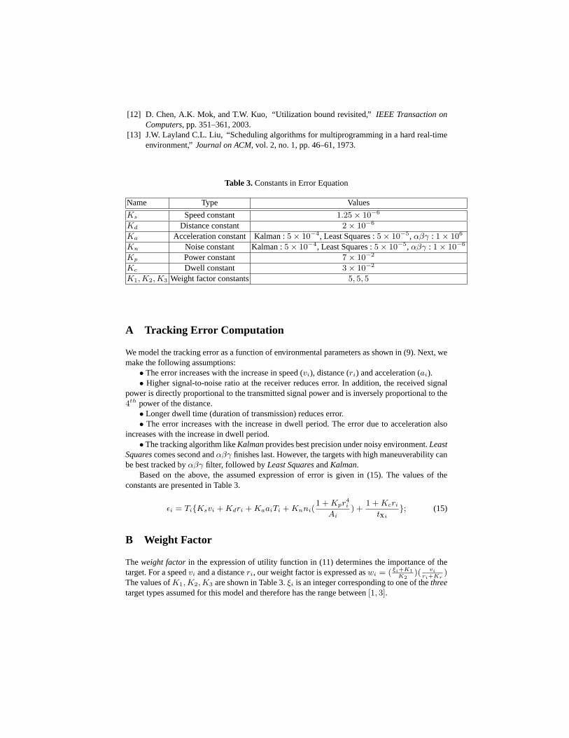
Table 3.Constants in Error Equation

Name Type Values

Ks Speed constant 1.25× 10−6

Kd Distance constant 2× 10−6

Ka Acceleration constant Kalman :5× 10−4, Least Squares :5× 10−5, αβγ : 1× 106

Kn Noise constant Kalman :5× 10−4, Least Squares :5× 10−5, αβγ : 1× 10−6

Kp Power constant 7× 10−2

Kc Dwell constant 3× 10−2

K1, K2, K3 Weight factor constants 5, 5, 5

A Tracking Error Computation

We model the tracking error as a function of environmental parameters as shown in (9). Next, wemake the following assumptions:

• The error increases with the increase in speed (vi), distance (ri) and acceleration (ai).• Higher signal-to-noise ratio at the receiver reduces error. In addition, the received signal

power is directly proportional to the transmitted signal power and is inversely proportional to the4th power of the distance.

• Longer dwell time (duration of transmission) reduces error.• The error increases with the increase in dwell period. The error due to acceleration also

increases with the increase in dwell period.• The tracking algorithm likeKalmanprovides best precision under noisy environment.Least

Squarescomes second andαβγ finishes last. However, the targets with high maneuverability canbe best tracked byαβγ filter, followed byLeast SquaresandKalman.

Based on the above, the assumed expression of error is given in (15). The values of theconstants are presented in Table 3.

εi = Ti{Ksvi + Kdri + KaaiTi + Knni(1 + Kpr4

i

Ai) +

1 + Kcri

txi

}; (15)

B Weight Factor

Theweight factorin the expression of utility function in (11) determines the importance of thetarget. For a speedvi and a distanceri, our weight factor is expressed aswi = ( ξi+K1

K2)( vi

ri+Kr)

The values ofK1, K2, K3 are shown in Table 3.ξi is an integer corresponding to one of thethreetarget types assumed for this model and therefore has the range between[1, 3].