Embed Size (px)
Citation preview

Adaptive RAKE Receiver Structures for Ultra Wide-Band Systems
A Thesis Submitted to the College
of Graduate Studies and Research
In Partial Fulfillment of the Requirements
For the Degree of Master of Science
In the Department of Electrical Engineering
University of Saskatchewan
Saskatoon
By
Quan Wan
© Copyright Quan Wan, December, 2005. All rights reserved

PERMISSION TO USE
In presenting this thesis in partial fulfillment of the requirement for a Postgraduate
degree from University of Saskatchewan, I agree that the Libraries of this
University may make it freely available for inspection. I further agree that
permission for copying of this thesis in any manner, in whole or in part, for
scholarly purposes may be granted by the professor or professors who supervised
my thesis work or, in their absence, by the Head of the Department or the Dean of
the College in which my thesis work was done. It is understood that any copying
for publication or use of this thesis or parts thereof for financial gain shall not by
allowed without my written permission. It is also understood that due recognition
shall be given to me and to the University of Saskatchewan in any scholarly use
which may be make of any material in my thesis.
Request for permission to copy or to make other use of material in this thesis in
whole or part should be addressed to:
Head of the Department of Electrical Engineering
University of Saskatchewan
Saskatoon, Saskatchewan, S7N 5A9
I

Abstract
Ultra wide band (UWB) is an emerging technology that recently has gained
regulatory approval. It is a suitable solution for high speed indoor wireless
communications due to its promising ability to provide high data rate at low cost
and low power consumption. Another benefit of UWB is its ability to resolve
individual multi-path components. This feature motivates the use of RAKE multi-
path combining techniques to provide diversity and to capture as much energy as
possible from the received signal.
Potential future and rule limitation of UWB, lead to two important
characteristics of the technology: high bit rate and low emitting power. Based on
the power emission limit of UWB, the only choice for implementation is the low
level modulation technology. To obtain such a high bit rate using low level
modulation techniques, significant inter-symbol interference (ISI) is unavoidable.
Three N (N means the numbers of fingers) fingers RAKE receiver structures are
proposed: the N-selective maximal ratio combiner (MRC), the N-selective MRC
receiver with least-mean-square (LMS) adaptive equalizer and the N-selective
MRC receiver with LMS adaptive combiner.
These three receiver structures were all simulated for N=8, 16 and 32.
Simulation results indicate that ISI is effectively suppressed. The 16-selective MRC
RAKE receiver with LMS adaptive combiner demonstrates a good balance between
performance, computation complexity and required length of the training sequence.
II

Due to the simplicity of the algorithm and a reasonable sampling rate, this structure
is feasible for practical VLSI implementations.
III

Acknowledgements
This thesis could not come through without the help of many wonderful people
around me. First of all, I would like to express my deepest sense of gratitude to my
supervisor, Dr. Anh Dinh, for his patient guidance, valuable advice and tremendous
technical and moral support. Working with him has been a true privilege. His
diligence, insights and enthusiasm demonstrate great scholars and dedicated
teachers. His ideas and inspirations have greatly helped the development of my
thesis. I really appreciate the countless times that he spent on discussions and
feedback on my work.
I would like to acknowledge TRLabs for supporting this research in the past two
years. I would also like to acknowledge my colleagues at TRLabs for making my
graduate studies and research work enjoyable and productive. The creation of the
outstanding research environment at TRLabs in Saskatoon is due to their tireless
efforts.
Finally, I would like to express my sincere gratitude to my father who always
encouraged me to face new challenges and never hesitated to provide me with ease
and comfort towards my educations.
IV

Dedication
To my dear parents
To my wife, Ying Cui, who has always been there for me and filled my life with
love and happiness
To my dear son, YingJia Wan
V

Table of Contents
Abstract ................................................................................................................... II
Acknowledgements ................................................................................................ IV
Dedication.................................................................................................................V
Table of Contents...................................................................................................VI
List of Tables.......................................................................................................... IX
List of Figures ..........................................................................................................X
List of Acronyms.................................................................................................XIII
Chapter 1 Introduction .......................................................................................... 1
1.1 Historical background .................................................................................. 1
1.2 Motivation .................................................................................................... 3
1.3 Problems and objectives ............................................................................... 5
1.4 Thesis overview............................................................................................ 8
Chapter 2 UWB Communication Technology ..................................................... 9
2.1 Definition of UWB ....................................................................................... 9
2.2 Advantages of UWB................................................................................... 11
2.3 Existing UWB system schemes.................................................................. 14
2.4 Channel characterization of UWB.............................................................. 17
Chapter 3 Receiver Signal Processing in the Presence of Multi-path ............. 24
3.1 RAKE receiver ........................................................................................... 24
3.2 Combating ISI ............................................................................................ 34
3.2.1 Optimum maximum-likelihood receiver ............................................. 35
3.2.2 Linear equalization .............................................................................. 36
VI

3.2.3 Decision-feedback equalization........................................................... 39
3.2.4 LMS adaptive equalization.................................................................. 40
Chapter 4 Proposed Receiver Structures ........................................................... 48
4.1 Basic requirements and considerations of receivers................................... 48
4.2 A simplified RAKE demodulation implementation ................................... 49
4.3 Channel estimation for RAKE demodulation............................................. 53
4.4 N-selective MRC RAKE receiver .............................................................. 57
4.5 N-selective MRC RAKE receiver with LMS adaptive equalizer............... 61
4.6 N-selective RAKE receiver with LMS adaptive combiner ........................ 67
Chapter 5 Simulation Set-up and Results .......................................................... 73
5.1 Simulation set-up........................................................................................ 73
5.1.1 Signal generator................................................................................... 74
5.1.2 UWB channel ...................................................................................... 75
5.1.3 Matched filter sampling and channel estimation................................. 77
5.1.4 N-selective MRC RAKE receiver and LMS adaptive equalizer ......... 78
5.1.5 N-selective RAKE receiver with LMS adaptive combiner ................. 79
5.2 Simulation results ....................................................................................... 79
5.3 Analysis and discussion.............................................................................. 90
Chapter 6 Conclusions and Future Work.......................................................... 95
6.1 Conclusions ................................................................................................ 95
6.2 Future work ................................................................................................ 97
Bibliography........................................................................................................... 99
Appendix A: Discrete-time model for a channel with ISI............................... 103
VII

Appendix B: Zero-forcing equalizer................................................................. 106
Appendix C: Mean-square-error (MSE) criterion linear equalizer .............. 108
Appendix D: Procedure to calculate a gradient vector................................... 110
VIII

List of Tables
Table 2-1: Unlicensed bands……………………………………………….....…..11
Table 2-2: The IEEE UWB channel characteristics………………………...…….20
Table 5-1: Parameters of different receiver structures…………………………….88
IX

List of Figures
Figure 2-1: UWB emission limit for indoor systems………..………………...... 10
Figure 2-2: UWB emission limit for outdoor hand-held systems…………..…… 10
Figure 2-3: Time divisions in THSS-UWB scheme…………………...………… 15
Figure 2-4: One realization of UWB channel model CM1……………………… 21
Figure 2-4: One realization of UWB channel model CM2………………….…... 21
Figure 2-6: One realization of UWB channel model CM3…………….……….. 22
Figure 2-7: One realization of UWB channel model CM4……………………… 22
Figure 3-1: Tapped delay line model of frequency-selective channel…………... 27
Figure 3-2: Optimum demodulator for wideband binary signals………………... 29
Figure 3-3: Model of binary digital communication system with Lth-order diversity……………………………………………………………. 33
Figure 3-4: Receiver structure for processing signal corrupted by ISI………….. 35
Figure 3-5: Linear transversal filter equalization structure……………….…….. 37
Figure 3-6: Block diagram of channel with zero-forcing equalizer………..……. 38
Figure 3-7: Structure of decision feedback equalizer………………….….……... 40
Figure 4-1: UWB transmission system model…………………………….…….. 49
Figure 4-2: The traditional RAKE demodulation implementation……….……... 50
Figure 4-3: A simplified RAKE demodulation implementation………………… 53
Figure 4-4: The number of single-path signal correlators in a UWB Rake receiver as a function of percentage energy capture for received waveforms in an office P (upper plot) and H (lower plot) representing typical “high SNR” and “low SNR” environment. In each plot, 49 measurement waveforms are used………………………………………………… 58
Figure 4-5: N- selective MRC RAKE receiver structure……………….……….. 61
X

Figure 4-6: N-selective MRC RAKE receiver with LMS adaptive equalizer…… 67
Figure 4-7: N-selective LMS RAKE receiver structure…………………………. 72
Figure 5-1: Block diagram of simulation…………………………………..……. 73
Figure 5-2: Simulink® block diagram of the signal generator………………….. 75
Figure 5-3: Block diagram of UWB channel……………………………………. 76
Figure 5-4: Simulink® block diagram of N-selective MRC RAKE receiver and LMS adaptive equalizer……………………………………..……... 78
Figure 5-5: Simulink® block diagram of N-selective RAKE receiver with LMS adaptive combiner………………………………………..………… 80
Figure 5-6: The BER for different pilot sequence…………………….…..…….. 81
Figure 5-7: The BER for N-selective MRC RAKE receiver structures….……… 82
Figure 5-8: The BER for LMS equalizers with different stages…….…..………. 83
Figure 5-9: The error signal for 8-selective MRC RAKE receiver with LMS adaptive equalizer……………………………………….…….……. 85
Figure 5-10: The error signal for 8-selective RAKE receiver with LMS adaptive combiner……………………………………………………………. 85
Figure 5-11: The error signal for 16-selective MRC RAKE receiver with LMS adaptive equalizer………………………………………………….. 86
Figure 5-12: The error signal for 16-selective RAKE receiver with LMS adaptive combiner……………………………………………………………. 86
Figure 5-13: The error signal for 32-selective MRC RAKE receiver with LMS adaptive equalizer………………………………………………….. 87
Figure 5-14: The error signal for 32-selective RAKE receiver with LMS adaptive combiner…………………………………………………..……….. 87
Figure 5-15: The BER for N-selective MRC RAKE receiver with LMS adaptive equalizer……………………………………………………….…… 89
Figure 5-16: The BER for N-selective RAKE receiver with LMS adaptive combiner…………………………………………………..……….. 90
Figure 5-17: The BER for three different receiver structures with N=8……….... 92
XI

Figure 5-18: The BER for three different receiver structures with N=16…….....92
Figure 5-19: The BER for three different receiver structures with N=32……….93
XII

List of Acronyms
AV audio and video
BER bit error rate
CMOS complementary metal oxide semiconductor
DD decision-directed
DFE decision-feedback equalizer
DSSS direct-sequence spread-spectrum
FCC Federal Communication Commission
FIR finite impulse response
IF intermediate frequency
ISI inter-symbol interference
LAN local area network
LMS least-mean-square
LOS line of sight
LTI linear time-invariant
MB multi-band
ML maximum-likelihood
MRC maximal ratio combiner
MSE mean-square-error
NLOS non-line of sight
OFDM orthogonal frequency division multiplexing
PAM pulse amplitude modulation
XIII

PAN personal area network
PPM pulse position modulation
RF radio frequency
RMS root-mean-square
SS spread spectrum
THSS time-hopping spread-spectrum
TR transmitted reference
UWB ultra wideband
WAN wide area network
WPAN wireless personal area networks
XIV

Chapter 1 Introduction
In this chapter, a brief history of ultra wideband (UWB) technology is described
first and then motivations of the research are given. Description of the problems
and objectives are also contained in this chapter.
1.1 Historical background
The concept of UWB communications originated in the early days of radio. In the
1900’s, the Marconi spark gap transmitter (the beginning of radio) communicated
by spreading a signal over a very wide bandwidth. This use of spectrum did not
allow for sharing. The communication world abandoned wideband communications
in favour of narrowband in order to share the available bandwidth. The government
of each country governs spectrum allocation and provides guidelines for radiated
power in the bandwidths of narrowband communication systems and for incidental
out of band radiated power.
The origin of ultra wideband technology stems from work in time-domain
electromagnetic begun in 1962 to fully describe the transient behaviour of a certain
class of microwave networks through their characteristic impulse response [1, 2].
The concept was indeed quite simple. Instead of characterizing a linear time-
invariant (LTI) system by the more conventional means of a swept frequency
response (i.e., amplitude and phase measurements versus frequency), an LTI system
could alternatively be fully characterized by its response to an impulsive excitation
-- the so-called impulse response h(t). In particular, the output y(t) of such a system
1

to any arbitrary input x(t) could be uniquely determined by the well-known
convolution integral:
∫∞
∞−−= duutxuhty )()()( (1.1)
However, it was not until the advent of the sampling oscilloscope (Hewlett-
Packard 1962) and the development of techniques for sub-nanosecond pulse
generation, to provide suitable approximations to an impulse excitation, that the
impulse response of microwave networks could be directly observed and measured.
Once impulse measurement techniques were applied to the design of wideband,
radiating antenna elements [1, 2], it quickly became obvious that short pulse radar
and communication systems could be developed with the same set of tools. While
at the Sperry Research Center, part of the Sperry Rand Corporation, Ross applied
these techniques to various applications in radar and communications [1, 2].
The invention of a sensitive, short pulse receiver to replace the cumbersome
time-domain sampling oscilloscope further accelerated system development. In
1973, Sperry was awarded the first UWB communications patent. Through the late
1980's, this technology was alternately referred to as base-band, carrier-free or
impulse communications. The term "ultra wideband" was not applied until 1989 by
the U.S. Department of Defence. By that time, UWB theory, techniques and many
hardware approaches had experienced nearly 30 years of extensive development.
By 1989, for example, Sperry had been awarded over 50 patents in the field
covering UWB pulse generation and reception methods, for applications such as
communications, radar, automobile collision avoidance, positioning systems, liquid
level sensing and altimetry [2].
2

On February 14th, 2002, the Federal Communication Commission (FCC) in the
US approved the use of this very controversial ultra-wideband technology for
commercial applications [3]. The targeted applications for UWB technology are
those that traditionally suffered from the multi-path fading effects like indoor high-
speed communications and positioning, ground penetrating radars, through-wall
and medical imaging systems or other security systems. In issuing its rules for
UWB, the FCC commissioners said that they were taking extreme care to avoid any
possible interference and believe that after a trial period, the commission will be
able to broaden the UWB applications permitted. UWB proponents believe that
UWB pulses will not cause interference with other narrowband applications
because the pulses continuously change frequencies and operate at extremely low
power levels.
1.2 Motivation
According to FCC’s definition, ultra wideband radio is a communication system
which utilizes a signal whose fractional bandwidth is greater than 0.2 or which
occupies 500 MHz or more of the spectrum.
Typical UWB radios communicate using sub-nanosecond pulses without a
carrier. The reason why a communication scheme using narrow pulse signals has
been proposed is because of their novel properties which possess advantages over
conventional narrow-band or wide-band signals. A UWB signal supplies that
bandwidth at a lower center frequency, which is advantageous for operation in
heavy multi-path environments and for penetration of materials. Resolvable multi-
3

path and the penetration capability enable a vision of potential UWB radio
applications in complex multi-path environments, including indoor wireless local
area network (LAN). Furthermore, the absence of a sinusoidal carrier may allow a
simpler radio architecture because no intermediate frequency (IF) stage is
necessary.
The benefits of an increasingly mobile lifestyle introduced by wireless
technologies in cell phones and home PCs resulted in a greater demand for the same
benefits in other consumer devices. Consumers have enjoyed the increased
convenience of wireless connectivity. They will soon demand it for video recording
and storage devices, for real-time audio and video (AV) streaming, interactive
gaming, and AV conferencing services as the need for digital media becomes more
predominate in the home. Many technologies used in the digital home, such as
digital video and audio streaming, require high bandwidth connections to
communicate. Considering the number of devices used throughout the digital home,
the bandwidth demand for wireless connectivity among these devices becomes very
large indeed. The wireless networking technologies developed for wireless
connecting PCs, such as Wi-Fi (IEEE 802.11a, b, g) and Bluetooth technology are
not optimized for multiple high-bandwidth usage models of a digital home.
Although data rates can reach 54 Mbps for Wi-Fi, for example, the technology has
limitations in a consumer electronics environment, including power consumption
and bandwidth. When it comes to connecting multiple consumer electronic (CE)
devices in a short-range network, or wireless personal area networks (WPAN), a
wireless technology is required to support multiple high data rate streams, consume
4

very little power, and maintain low cost, while fitting into a very small physical
package, such as a PDA or a cell phone. The emerging UWB wireless technology
and silicon developed for UWB applications offer a compelling solution.
1.3 Problems and objectives
UWB differs substantially from conventional narrowband radio frequency (RF) and
spread spectrum technologies (SS), such as Bluetooth Technology and 802.11a/g.
UWB uses an extremely wide band of RF spectrum to transmit data. In doing so,
UWB is able to transmit more data in a given period of time than traditional
technologies. The potential data rate over a given RF link is proportional to the
bandwidth of the channel and the logarithm of the signal-to-noise ratio as stated in
the Hartley-Shannon law
)1(log2 NSBC += (1.2)
where:
C = Maximum channel capacity, in bits per second.
B = Channel bandwidth, in Hertz.
S = Signal power, in watts.
N = Noise power, in watts.
RF design engineers typically have little control over bandwidth parameters as
they are dictated by FCC regulations that stipulate the allowable bandwidth of the
signal for a given radio type and application. Bluetooth Technology, 802.11a/g Wi-
Fi, cordless phones, and numerous other devices are relegated to the unlicensed
frequency bands at 900 MHz, 2.4 GHz, and 5.1 GHz.
5

Each radio channel is constrained to occupy only a narrow band of frequencies,
relative to what is allowed for UWB. UWB is a unique and new usage of a recently
legalized frequency spectrum. UWB radios can use frequencies from 3.1 GHz to
10.6 GHz—a band more than 7 GHz wide. Each radio channel can have a
bandwidth of more than 500 MHz. To allow for such a large signal bandwidth, the
FCC put in place severe broadcast power restrictions. By doing so, UWB devices
can make use of an extremely wide frequency band while not emitting enough
energy to be noticed by nearby narrower band devices, such as the 802.11a/g
radios. This spectrum sharing allows devices to obtain very high data throughput,
but they must be within close proximity. Strict power limits mean the radios
themselves must be low power consumers. Because there is no need to emit a high
power signal, it is feasible to develop cost-effective CMOS implementations of
UWB radios in place of expensive high power components. With the characteristics
of low power, low cost, and very high data rates at a limited range, UWB is
positioned to address the market for high-speed WPAN.
Potential future and rule limitation of UWB, lead to two important
characteristics of the technology: high bit rate and low emitting power. Based on
the power emission limit of UWB, the only choice for implementation is using low
level modulation technology. To obtain such a high bit rate using low level
modulation techniques, the required symbol period is very small. According to the
UWB channel model from IEEE P802.15 [4], there is a root-mean-square (RMS)
delay spread of approximately 15ns for a 4-10 meter range with a non line-of-sight
transmission. This spread indicates that a significant inter-symbol interference (ISI)
6

is unavoidable. The traditional RAKE receiver structure to collect multi-path
energy in UWB systems does not combat ISI very well. Some published results on
UWB have neglected this problem as most performance analyses employ a RAKE
receiver under the assumption that channel delay spreads are much less than system
symbol time [5, 24, 27, 29].
Still for a 4-10 meter range with a non line-of-sight transmission in the UWB
channel model from IEEE P802.15, the average number of significant paths
capturing greater than 85% energy is more than sixty. How could the multi-path
signal’s energy be captured effectively for a reasonable cost? How could the dense
multi-path channel parameters be measured in the high data rate application
environment?
The first objective is to find a method to estimate the channel parameters and
gather multi-path energy with the low computation complexity. The second
objective is to find suitable equalization technologies to suppress the significant
inter-symbol interference. The overall objective of this research is to propose low
cost UWB receiver structures with low complexity and a low sampling rate that can
achieve satisfactory performance under a significant ISI.
In this thesis, the sample and effective sliding correlation algorithm is applied
for UWB channel estimation. An analog and digital hybrid implementation of a
RAKE receiver structure is proposed. Two schemes for suppressing ISI, LMS
equalization and LMS combining, are developed. Simulations are performed using
the popular simulation tool, MATLAB Simulink®. According to the simulation
results, the objectives are achieved.
7

1.4 Thesis overview
This chapter provides a brief historical background on UWB communication
systems. Motivation, problems and objectives are also discussed. The rest of this
thesis is organized as follows.
Chapter 2 provides a definition of UWB signal. Advantages of this technology
are also discussed. Existing UWB system schemes are briefly reviewed and channel
characterization of UWB is introduced. Chapter 3 deals with signal processing
technologies in the presence of multi-path, RAKE multi-path combining techniques
and different equalization techniques. Chapter 4 describes the proposed receiver
structures. Chapter 5 focuses on simulation set-up. This chapter also provides
analysis and discussion of the simulation results. Finally, conclusions on the
accomplished research objectives are summarized and research topics for future
work are suggested in Chapter 6.
8

Chapter 2 UWB Communication Technology
In this chapter, the official definition and advantages of UWB are given. Basic
concepts of several current main stream UWB system schemes are introduced
subsequently. Finally UWB channel modes are described.
2.1 Definition of UWB
The UWB technology was often referred to as base-band, carrier-free or short
impulse. But there was not a clear definition of UWB until the Federal
Communications Commission’s Report and Order [3], issued on Feb 2002, gives an
official definition for UWB. According to this definition, an UWB signal is any
signal whose fractional bandwidth is greater than 0.20 or occupies 500 MHz or
more of the spectrum. The formula proposed by the FCC for calculating fractional
bandwidth is
)/()(2 LHLH ffff +− ,
where is the upper frequency of the –10 dB emission point and is the lower
frequency of the –10 dB emission point. The center frequency of the transmission
was defined as the average of the upper and lower –10 dB points, i.e.,
. Meanwhile UWB signals must meet the spectrum mask shown in
Fig. 2-1 and Fig. 2-2.
Hf Lf
2/)( LH ff +
According to the FCC’s rules, there is 7.5 GHz bandwidth (3.1 GHz—10.6
GHz) available for UWB communications and measurement systems. The allowed
power emission level is -41.3 dBm/MHz. The equipment must be designed to
9

0.96 1.61
1.99 3.1 10.6
GPS Band
Figure 2-1: UWB emission limit for indoor systems
Figure 2-2: UWB emission limit for outdoor hand-held systems
0.96 1.61
1.993.1 10.6
GPS Band
ensure that the operation can only occur indoors or it must consist of hand held
devices that may be employed for such activities as peer-to-peer operation. A
comparison with the other unlicensed bands currently available in the US is shown
in Table 1.
10

Table 2-1: Unlicensed bands
Unlicensed bands Frequency of operation Bandwidth
ISM at 2.4GHz 2.4000-2.4835 GHz 83.5MHz
U-NII at 5GHz 5.15-5.35GHz
5.725-5.825GHz
300MHz
UWB 3.1-10.6GHz 7,500MHz
Given the recent spectral allocation and the new definition of UWB adopted by
FCC, UWB is not only just considered as a technology anymore, but also available
spectrum for unlicensed use. This means that any transmission signal that meets the
FCC requirements for UWB spectrum is acceptable. This, of course, is not just
restricted to impulse radios or high speed spread spectrum radios pioneered by
companies so far, but opened to any technology that utilizes more than 500MHz
spectrum in the allowed spectral mask.
2.2 Advantages of UWB
Because UWB waveforms are of such short time duration, they have some unique
properties. In communications, for example, UWB pulses can be used to provide
extremely high data rate performance in multi-user network applications. For radar
applications, these same pulses can provide a very fine range resolution and a
precision distance and positioning measurement capability.
These short duration waveforms are relatively immune to multi-path effects
compared to normal narrow band systems as observed in mobile and in-building
11

environments. As a result, UWB systems are particularly well suited for high-speed
wireless applications.
As bandwidth is inversely related to pulse duration, the spectral extent of these
waveforms can be made quite large. With proper engineering design, resultant
energy densities (i.e., transmitted Watts of power per unit Hertz of bandwidth) can
be quite low. This low energy density is translated into a low probability of
detection RF signature. The low probability of detection signature is of particular
interest for military applications; meanwhile, it also produces minimal interference
to proximity systems and minimal RF health hazards, which is a significant benefit
for both military and commercial applications.
Among the most important advantages of UWB technology, however, are those
of low system complexity and low cost. UWB systems can be made nearly "all-
digital," with minimal RF or microwave electronics. Because of the inherent RF
simplicity of UWB designs, these systems are highly frequency adaptive, enabling
them to be positioned anywhere within the RF spectrum. This feature avoids
interference to existing services, while fully using the available spectrum.
In summary, UWB presents a compelling solution to many of the challenges
facing today's wireless industry and applications. These include the following [30]:
• Low radiated power: UWB is limited by regulation to power levels that
are a tiny fraction of other radio technologies, with possible health benefits
and adaptation to sensitive environments, such as hospitals and airports.
12

• Speed - The same UWB device can scale from speeds far in excess of
current communication networks, to very low speed (and low power)
applications, such as meter reading.
• Multiple channels - UWB can support hundreds of simultaneous channels,
compared to three for 802.11b, or ten for 802.11a.
• Simultaneous networking - This technology can function as a personal
area network (PAN), a local area network (LAN), and a wide area network
(WAN), simultaneously. It is the equivalent of Bluetooth, 802.11, and 3G
converging, but in a single network, with a single device.
• Lower cost and complexity - Devices using RF spectrum require a real
radio receiver and so are more complex in terms of components, higher cost,
and consume significantly more power than UWB which operates at lower
power, and requires fewer components.
• Greater security - The inherent digital nature of UWB transmission,
coupled with its operation in the lower power level, makes UWB perhaps
the most secure means of wireless transmission available.
• Co-existence - Because UWB signals can co-exist with conventional RF
carriers, the technology will open up vast new communication possibilities
by creating a new communication medium that peacefully coexists with
existing technologies.
UWB is an RF wireless technology and, as such, is still subject to the same laws
of physics as other RF technologies. Thus, there are obvious tradeoffs to be made in
13

signal-to-noise ratio versus bandwidth, range versus speed, and average power
levels, and so on.
2.3 Existing UWB system schemes
There are four popular UWB system schemes: time-hopping spread-spectrum ultra
wideband (THSS-UWB); direct-sequence spread-spectrum ultra wideband (DSSS-
UWB); multi-band orthogonal frequency division multiplexing ultra wideband
(MB-OFDM-UWB) and transmitted reference ultra wideband (TR-UWB).
• Time-hopping spread-spectrum ultra wideband
In THSS-UWB, the transmitted signal for one user using binary
antipodal modulation can be defined as [6]
)(tSTH
⎣ ⎦∑∞
−∞=
−−−=j
NjcjftrTH SDTcjTtwtS )21)(()( (2.1)
where denotes the transmitted pulse form that has a maximum amplitude of
one, a duration of and is transmitted with a repetition period . The position of
a transmitted pulse within each repetition period is determined by a pseudorandom
code which selects one of the slots, each having a duration of . The
pseudorandom code takes integer value between 0 and
)(twtr
cT fT
jc N cT
jc 1−N and it is assumed
that . Moreover, fc TNT ≤ }1,0{∈D is a data stream and ⎣ ⎦x denotes the integer
part of x. A new bit starts with j = 0 mod . Each information bit is transmitted
with pulses and has a duration of
SN
SN fSS TNT = . Figure 2-3 shows the time
divisions.
14

Figure 2-3: Time divisions in THSS-UWB scheme
• Direct-sequence spread-spectrum ultra wideband
A DSSS-UWB system is basically identical to an ordinary DSSS system except
that the bandwidth spreading effect is achieved by pulse shaping. Similar to THSS-
UWB above, DSSS-UWB is defined as
⎣ ⎦∑∞
−∞=
−−=j
NjjmtrDS DSDnjTtwtS )21()()( (2.2)
where is a pseudorandom code that takes values {±1}. Each information bit
consists of pulses and has a duration of
jn
DSN mDSb TNT = .
The flexibility provided by the FCC ruling greatly expands the design options
for UWB communication systems. Designers are free to use a combination of sub-
bands within the spectrum to optimize system performance, power consumption
and design complexity. UWB systems can still maintain the same low transmit
power as if they were using the entire bandwidth by interleaving the symbols across
these sub-bands [7].
• Multi-band orthogonal frequency division multiplexing ultra wideband
15

The MB-OFDM-UWB system transmits data simultaneously over multiple
carriers spaced apart at precise frequencies by mean of OFDM modulation
techniques. Beneficial attributes of MB-OFDM include high spectral flexibility and
resiliency to RF interference and multi-path effects.
Regardless of present or future spectral allocations and emissions restrictions in
various regions of the world, MB-OFDM is capable of complying with local
regulations by dynamically turning off certain tones or channels using software.
This flexibility, not demonstrated by other system schemes, enables worldwide
adoption of UWB systems.
• Transmitted reference ultra wideband
To circumvent the drawbacks of RAKE receivers, e.g. channel estimation or
finding a suitable template pulse form for correlation, TR-UWB schemes are well
suited. A TR-UWB system transmits a doublet every seconds. The first pulse of
each doublet is information free, and the second delayed pulse that is modulated by
pulse amplitude modulation (PAM), or pulse position modulation (PPM) and
delayed by seconds carries the user’s information. Denote the pulse by
with duration and the binary PAM symbol by
ST
dT )(twtr
pT }1,0{∈D . The transmitted signal
can be described by [8]
)]()21()([)( dStrj
jStrTR TjTtwDjTtwtS −−−+−= ∑∞
−∞=
(2.3)
Reasonably assume and pd TT > Spd TTT <+ , meaning the first and second pulses
do not interfere each other before propagating through a channel. However, large
pulse spacing inevitably sacrifices data rate for good performance, especially when
16

the channel spread is very large [4]. Meanwhile, the first pulse may severely
interfere with the second pulse and cause inter-pulse interference.
2.4 Channel characterization of UWB
The IEEE UWB channel model is based on the Saleh–Valenzuela model where
multi-path components arrive in clusters [4, 9]. In this model, a lognormal
distribution was used rather than a Rayleigh distribution for the multi-path gain
magnitude. In addition, independent fading is assumed for each cluster as well as
each ray within the cluster. Therefore, the multi-path model consists of the
following discrete time impulse response:
∑∑= =
−−=L
l
K
k
ilk
il
ilkii TtXth
0 0,, )()( τδα (2.4)
where are the multi-path gain coefficients, is the delay of the l}{ ,i
lkα }{ ilT th cluster,
is the delay of the k}{ ,i
lkτth multi-path component relative to the lth cluster arrival
time , }{ represents the log-normal shadowing, and i refers to the i}{ ilT iX th
realization of the channel. Finally, the model uses the following definitions:
Tl = the arrival time of the first path of the l-th cluster.
τk,l = the delay of the k-th path within the l-th cluster relative to the first path
arrival time, Tl.
Λ = cluster arrival rate.
λ = ray arrival rate, i.e., the arrival rate of the paths within each cluster.
17

By definition, 0,0 =lτ . The distribution of cluster arrival time and the ray arrival
time are given by
0)],(exp[)|( 11 >−Λ−Λ= −− lTTTTp llll (2.5)
0)],(exp[)|( ),1(,),1(, >−−= −− kp lklklklk ττλλττ (2.6)
The channel coefficients are defined as follow:
lkllklk p ,,, βξα = ,
),(Normal)(10log20 22
21,, σσμβξ +∝ lklkl , or 20/)(
,21,10 nn
lkllk ++= μβξ
where and are independent and
correspond to the fading on each cluster and ray respectively.
),0Normal( 211 σ∝n ),0Normal( 2
22 σ∝n
γτβξ //0
2
,,lkl eeE T
lkl−Γ−Ω=⎥⎦
⎤⎢⎣⎡
(2.7)
where Tl is the excess delay of bin l and 0Ω is the mean energy of the first path of
the first cluster, and is equiprobable +/-1 to account for signal inversion due to
reflections. The μ
lkp ,
k,l is given by
20)10ln()(
)10ln(/10/10)ln(10 2
221,0
,σσγτ
μ+
−−Γ−Ω
= lkllk
T (2.8)
In the above equations, lξ reflects the fading associated with the lth cluster, and
lk ,β corresponds to the fading associated with the kth ray of the lth cluster. Note
that, a complex tap model is not adopted here. The complex base-band model is a
natural fit for narrowband systems to capture channel behavior independently of
carrier frequency, but this motivation breaks down for UWB systems where a real-
valued simulation at RF may be more natural.
18

Finally, since the log-normal shadowing of the total multi-path energy is
captured by the term, , the total energy contained in the terms { } is
normalized to unity for each realization. This shadowing term is characterized by
the following:
iX ilk ,α
),0(Normal)(10log20 2xiX σ∝ .
As shown above, there are 7 key parameters that define the model:
Λ = cluster arrival rate.
λ = ray arrival rate, i.e., the arrival rate of path within each cluster.
Γ = cluster decay factor.
γ = ray decay factor.
1σ = standard deviation of cluster lognormal fading term (dB).
2σ = standard deviation of ray lognormal fading term (dB).
xσ = standard deviation of lognormal shadowing term for total multi-path
realization (dB).
These parameters are found by trying to match important characteristics of the
channel. Since it is difficult to match all possible channel characteristics, the main
characteristics of the channel that are used to derive the above model parameters
are chosen to be the following:
• Mean excess delay
• RMS delay spread
• Number of multi-path components which is defined as the number of multi-
path arrivals that are within 10 dB of the peak multi-path arrival
19

There are four distinguished models:
CM1: This model is based on line of sight (LOS) (0-4m) channel
measurements.
CM2: This model is based on non-line of sight (NLOS) (0-4m) channel
measurements.
CM3: This model is based on non-line of sight (NLOS) (4-10m) channel
measurements.
CM4: This model is generated to fit a 25 nsec RMS delay spread to represent
an extreme no-line of sight (NLOS) multi-path channel.
The following table lists some initial model parameters for a couple of different
channel characteristics that were found through measurement data.
Table 2-2: The IEEE UWB channel characteristics [4]
Model Parameters CM 1 CM 2 CM 3 CM 4 Λ (1/nsec) 0.0233 0.4 0.0667 0.0667 λ (1/nsec) 2.5 0.5 2.1 2.1 Γ 7.1 5.5 14.00 24.00 γ 4.3 6.7 7.9 12
1σ (dB) 3.3941 3.3941 3.3941 3.3941
2σ (dB) 3.3941 3.3941 3.3941 3.3941
xσ (dB) 3 3 3 3 Model Characteristics Mean excess delay (nsec) ( mτ ) 5.0 9.9 15.9 30.1 RMS delay (nsec) ( rmsτ ) 5 8 15 25 NP10dB 12.5 15.3 24.9 41.2 NP (85%) 20.8 33.9 64.7 123.3 Channel energy mean (dB) -0.4 -0.5 0.0 0.3 Channel energy std (dB) 2.9 3.1 3.1 2.7
20

Figure 2-4: One realization of UWB channel model CM1
Nor
mal
ized
sign
al a
mpl
itude
Figure 2-5: One realization of UWB channel model CM2
Nor
mal
ized
sign
al a
mpl
itude
21

Figure 2-6: One realization of UWB channel model CM3
Nor
mal
ized
sign
al a
mpl
itude
Figure 2-7: One realization of UWB channel model CM4
Nor
mal
ized
sign
al a
mpl
itude
22

One realization of each channel model impulse response is shown below
(continuous-time model). From Figure 2-3 the multi-path delay spread for CM1 is
about 90 ns. For CM2 in Figure 2-4 the multi-path delay spread increase to about
120 ns. For CM3 in Figure 2-5 this value is about 200ns and for CM4 in Figure 2-6
it is almost 330ns.
23
Chapter 3 Receiver Signal Processing in the
Presence of Multi-path In this chapter, introduction of the RAKE receiver is given at the beginning. Then a
description of ISI and some of the most used methods to combat ISI are introduced
subsequently.
3.1 RAKE receiver
The extremely large bandwidth of UWB signals means that the UWB channel is
highly frequency selective. According to the introduction of UWB channel model
in Chapter 2, a large number of multi-path components arrive at the receiver with
different time delays. This means that large losses in the receiver’s performance
will occur if a method of combating this frequency selective dense multi-path is not
employed. However, the extremely narrow pulses used for UWB transmission lead
to inherent path diversity (i.e., independent fading of different multi path
components). This implies that the received UWB signal contains a significant
number of resolvable multi path components which suggests a RAKE type receiver
to coherently combine them [5, 10]. This significantly reduces the fading effects
and the resulting reduction of fading margins in link power budgets leads to
reduced transmission power requirements.
The RAKE receiver was invented by Price and Green in 1958 [11]. The receiver
is used to achieve multi-path diversity by collecting signal energy from each
received path using a delay line structure [12]. In spread spectrum communications,
24

the bandwidth of the spread signal is usually larger than the channel coherence
bandwidth. If the bandwidth of the transmitted signal is large enough, it is possible
to resolve multi-path components into separate signals. In such a case, the actual
channel can be modeled as a tapped delay line with time varying tap coefficients
[13].
Now suppose that W is the bandwidth occupied by real band-pass signal, then
the band occupancy of the equivalent low-pass signal is)(tsl Wf21
≤ . Since
is band-limited to
)(tsl
Wf21
≤ , according to the sampling theorem can be
expressed as
)(tsl
[ ])/(
)/(sin)()(WntW
WntWWnsts
nll −
−= ∑
+∞
−∞= ππ (3.1)
The Fourier transform of is )(tsl
⎪⎪⎭
⎪⎪⎬
⎫
⎪⎪⎩
⎪⎪⎨
⎧
>
≤=
∑∞
−∞=
−
)21(0
)21()/(1
)(/2
Wf
WfeWnsWfS n
Wfnjl
l
π
(3.2)
The noiseless received signal through a frequency-selective channel is expressed in
the form
∫∞
∞−= dfefStfCtr ftj
llπ2)();()( (3.3)
where is the time-variant transfer function. Substitution for from
(3.2) into (3.3) yields
);( tfC )( fSl
∫∑∞
∞−
−∞
−∞=
= dfetfCWnsW
tr Wntfj
nll
)/(2);()/(1)( π
25

);/()/(1 tWntcWnsW n
l −= ∑∞
−∞=
(3.4)
where );( tc τ is the time-variant impulse response. It is observed that equation (3.4)
has the form of a convolution sum. Hence, it can be expressed in an alternative
form as:
);/()/(1)( tWncWntsW
trn
ll ∑∞
−∞=
−= (3.5)
It is convenient to define a set of time-variable channel coefficients as
);(1)( tWnc
Wtcn = (3.6)
Then Equation (3.5) expressed in terms of these channel coefficients become
∑∞
−∞=
−=n
lnl Wntstctr )/()()( (3.7)
The form for the received signal in Equation (3.7) implies that the time-variant
frequency-selective channel can be modeled or represented as a tapped delay line
with tap spacing 1/W and tap weight coefficients . In fact, it is deduced from
Equation (3.7) that the low-pass impulse response for the channel is
)}({ tcn
∑∞
−∞=
−=n
n Wntctc )/()();( τδτ (3.8)
and the corresponding time-variant transfer function is
∑∞
−∞=
−=n
Wfnjn etctfC /2)();( π (3.9)
Thus, with an equivalent low-pass-signal having a bandwidth W21 , one
achieves a resolution of 1/W in the multi-path delay profile. Since the total multi-
26

path spread is , for all practical purposes, the tapped delay line model for the
channel can be truncated at
mT
⎣ ⎦ 1+= WTL m taps. Then the noiseless received signal
can be expressed in the form
∑=
−=L
nlnl Wntstctr
1)/()()( (3.10)
The truncated tapped delay line model is shown in Figure 3-1. The time-variant
tap weights are complex-valued stationary random processes. Since
represent the tap weights corresponding to the L different delays
)}({ tcn )}({ tcn
Wn /=τ ,
, the uncorrelated scattering assumption implies that are
mutually uncorrelated. When are Gaussian random processes, they are
statistically independent.
Ln ,,2,1 K= )}({ tcn
)}({ tcn
1/W 1/W 1/W 1/W )(tsl
)(1 tc )(2 tc )(3 tc )(tcL
∑
Additive noise z(t)
)()()()(1
tzWktstctr
L
klkl +−= ∑
=
Figure 3-1: Tapped delay line model of frequency-selective channel
27
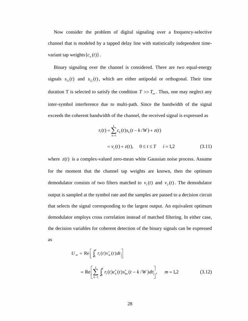
Now consider the problem of digital signaling over a frequency-selective
channel that is modeled by a tapped delay line with statistically independent time-
variant tap weights . )}({ tcn
Binary signaling over the channel is considered. There are two equal-energy
signals and , which are either antipodal or orthogonal. Their time
duration T is selected to satisfy the condition . Thus, one may neglect any
inter-symbol interference due to multi-path. Since the bandwidth of the signal
exceeds the coherent bandwidth of the channel, the received signal is expressed as
)(1 tsl )(2 tsl
mTT >>
)()/()()(1
tzWktstctrL
klikl +−=∑
=
),()( tztvi += Tt ≤≤0 2,1=i (3.11)
where is a complex-valued zero-mean white Gaussian noise process. Assume
for the moment that the channel tap weights are known, then the optimum
demodulator consists of two filters matched to and . The demodulator
output is sampled at the symbol rate and the samples are passed to a decision circuit
that selects the signal corresponding to the largest output. An equivalent optimum
demodulator employs cross correlation instead of matched filtering. In either case,
the decision variables for coherent detection of the binary signals can be expressed
as
)(tz
)(1 tv )(2 tv
⎥⎦⎤
⎢⎣⎡= ∫ ∗T
mlm dttvtrU0
)()(Re
,)/()()(Re1
0 ⎥⎦
⎤⎢⎣
⎡−= ∑ ∫
=
∗∗L
k
T
lmkl dtWktstctr 2,1=m (3.12)
28
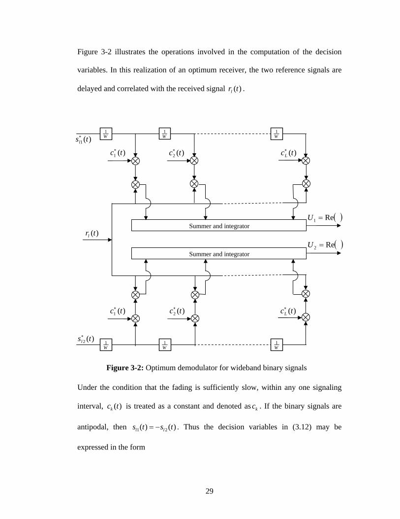
Figure 3-2 illustrates the operations involved in the computation of the decision
variables. In this realization of an optimum receiver, the two reference signals are
delayed and correlated with the received signal . )(trl
W1 W
1W1
Summer and integrator
Summer and integrator
W1
W1
W1
)(1 tsl∗
)(2 tsl∗
)(trl
)(1 tc∗
)(1 tc∗
)(2 tc∗
)(2 tc∗
)(tcL∗
)(tcL∗
( )Re2 =U
( )Re1 =U
Figure 3-2: Optimum demodulator for wideband binary signals
Under the condition that the fading is sufficiently slow, within any one signaling
interval, is treated as a constant and denoted as . If the binary signals are
antipodal, then . Thus the decision variables in (3.12) may be
expressed in the form
)(tck kc
)()( 21 tsts ll −=
29

⎥⎦
⎤⎢⎣
⎡−= ∑ ∫
=
∗∗L
k
T
llk dtWktstrcU1
0 1 )/()(Re (3.13)
Suppose the transmitted signal is , then the received signal is )(1 tsl
)()/()(1
1 tzWktsctrL
klkl +−=∑
=
Tt ≤≤0 (3.14)
Substitution of Eq.(3.14) into Eq.(3.13) yields
⎥⎦
⎤⎢⎣
⎡−−= ∑ ∫∑
=
∗
=
∗L
k
T
ll
L
nnk dtWktsWntsccU
10 11
1)/()/(Re
(3.15) ⎥⎦
⎤⎢⎣
⎡−+ ∑ ∫
=
∗∗L
k
T
lk dtWktstzc1
0 1 )/()(Re
If inter-pulse interference is neglected, the resulting signals have the property
,0)/()/(0 11 =−−∫ ∗T
ll dtWktsWnts nk ≠ (3.16)
Then Eq.3.15 can be simplified to
⎥⎦
⎤⎢⎣
⎡−−= ∫∑ ∗
=
T
ll
L
kk dtWktsWktscU
0 111
2 )/()/(Re
⎥⎦
⎤⎢⎣
⎡−+ ∑ ∫
=
∗∗L
k
T
lk dtWktstzc1
0 1 )/()(Re
⎟⎠
⎞⎜⎝
⎛+= ∑∑
==
L
kkk
L
kk N
11
2Re ααε (3.17)
where and kjkk ec φα −=
∫ −−= ∗T
ll dtWktsWkts0 11 )/()/(ε (3.18)
∫ −= ∗T
lj
k dtWktstzeN k
0 1 )/()(φ (3.19)
30

In effect, the tapped delay line demodulator attempts to collect the signal energy
from all received signal paths that fall within the span of the delay line and carry
the same information. Its action is somewhat analogous to an ordinary garden rake
and, consequently, the name “RAKE demodulator” has been coined for this
demodulator structure by Price and Green [11].
It is apparent that the tapped delay line model with statistically independent tap
weights provides L replicas of the same transmitted signal at the receiver. Hence, a
receiver that processes the received signal in an optimum manner will achieve the
performance of an equivalent Lth-order diversity communication. The L replicas of
the transmitted signal at the receiver can be considered as carrying the same
information-bearing signal passed through L diversity channels. Each channel is
assumed to be frequency-nonselective and slowly fading. The fading processes
among the L diversity channels are assumed to be mutually statistically
independent. The signal in each channel is corrupted by an additive zero-mean
white Gaussian noise process. The noise processes in the L channels are assumed to
be mutually statistically independent. Thus the equivalent low-pass received signals
for the L channels can be expressed in the form
),()()( tztsetr kkmj
klkk += − φα ,,,2,1 Lk K= 2,1=m (3.20)
where { }kjke
φα − represent the attenuation factors and phase shifts for the L
channels, denotes the m)(tskmth signal transmitted on the kth channel, and
denotes the additive white Gaussian noise on the k
)(tzk
th channel. All signals in the set
have the same energy. { )(tskm }
31

The optimum demodulator for the signal received from the kth channel consists
of two matched filters, one having the impulse response
)()( 11 tTsth kk −= ∗ (3.21)
and the other having the impulse response
)()( 22 tTsth kk −= ∗ (3.22)
Of course, if BPSK is the modulation method used to transmit information, then
. Consequently, only a single matched filter is required for BPSK.
Following the matched filters is a combiner that forms the two decision variables.
The combiner that achieves the best performance is one in which each matched
filter output is multiplied by the corresponding complex-valued (conjugate) channel
gain . The effect of this multiplication is to compensate for the phase shift in
the channel and to weight the signal by a factor that is proportional to the signal
strength. Thus, a strong signal carries a larger weight than a weak signal. After the
complex-valued weighting operation is performed, two sums are formed. One
consists of the transmitted 0. The second consists of the real part of the outputs
from the matched filters corresponding to a transmitted 1. This optimum combiner
is called a maximal ratio combiner (MRC) by Brennan [19]. Of course, the
realization of this optimum combiner is based on the assumption that the channel
attenuations { and the phase shifts
)()( 21 tsts kk −=
kjke
φα
}ka { }kφ are known. A block diagram illustrating
the model for the binary digital communication system described above is shown in
Figure 3-3.
If the modulation is BPSK, the output of the maximal ratio combiner can be
expressed as a single decision variable in the form
32

⎟⎠
⎞⎜⎝
⎛+= ∑∑
==
L
kkk
L
kk NU
11
2Re ααε (3.23)
where
∫ ∗=T
kk dttsts0 11 )()(ε (3.24)
∫ ∗=T
kkj
k dttstzeN k
0 1 )()(φ (3.25)
It is noticed that Eq.3.23 is identical to the decision variable given in Eq.3.17,
which corresponds to the output of the RAKE demodulation. Consequently, the
RAKE demodulator with perfect estimates of the channel tap weights is equivalent
to a maximal ratio combiner in a system with Lth-order diversity.
)(2 tz
Figure 3-3: Model of binary digital communication system with Lth-order diversity.
Channel 1 1
1φα je−
)()(
12
11
tsts
Receiver
1
Channel 1 2
2φα je−
)()(
22
21
tsts
Receiver
2
Channel 1 Lj
Le φα − )()(
2
1
tsts
l
l Receiver
L
)(1 tz
)(tzL
Combiner
Output Decision Variables
.
.
.
.
.
.
.
.
.
.
.
.
.
.
33

3.2 Combating ISI
The RAKE demodulator described above is an optimum demodulator based on the
condition that the bit interval , i.e., there is negligible ISI. When the
condition is not satisfied, the RAKE demodulator output is corrupted. If ISI is left
uncompensated, high error rate will occur. The detailed information about the
equivalent discrete-time model for a channel with ISI is in Appendix A. The
solution to the ISI problem is to design a receiver that employs a means for
compensating or reducing the ISI in the received signal. The compensator for the
ISI is called an equalizer. From the potential future and rule limitation of UWB, it
is well known that there are two important characteristics of UWB: high bit rate and
low emitting power. Based on the power emission limit of UWB one can only
choose low level modulation technology. To obtain such high bit rate with low
level modulation techniques, the result is very small symbol period. According to
the UWB channel models from IEEE P802.15 [4], there is a RMS delay spread of
approximately 15ns for a 4-10 meter range with a non line-of-sight transmission.
This spread indicates that a significant inter-symbol interference is unavoidable. In
such a case, an equalizer is required to suppress ISI. At the receiver, after the signal
is demodulated to base-band, it may be processed by the RAKE, followed by an
equalizer to suppress the ISI. The RAKE output is sampled at bit rate, and these
samples are passed to the equalizer. This structure is shown in Figure 3-4. There are
several types of equalization methods being extensively used. One is based on the
maximum-likelihood (ML) sequence detection criterion, which is optimum from a
probability of error viewpoint. A second equalization method is based on the use of
mb TT >>
34

a linear filter with adjustable coefficients. A third equalization method that is
described exploits the use of previously detected symbols to suppress ISI in the
present symbol being detected; this is called decision-feedback equalization. All
these equalization methods are now described in detail.
RAKE demodulator Sampler Equalizer Output
Symbol-rate clock
Received base-band
signal
Figure 3-4: Receiver structure for processing signal corrupted by ISI
3.2.1 Optimum maximum-likelihood receiver
The received base-band signal can be expressed as
)()()( tznTthItrn
nl +−= ∑ (3.26)
where is the information sequence, represents the response of the channel
to the input signal pulse and represents the additive white Gaussian
noise. The maximum-likelihood estimates of the symbols
{ }nI )(th
)(tg )(tz
[ ]pp III ,,, 21 K≡Ι are
those that maximize this quantity:
∑∑∑ −∗∗ −⎟
⎠
⎞⎜⎝
⎛=Ι
n mmnmn
nnnp xIIyICM Re2)( (3.27)
where
35

dtnTthtrnTyy ln ∫∞
∞−
∗ −=≡ )()()( (3.28)
dtnTththnTxxn ∫∞
∞−
∗ +=≡ )()()( (3.29)
In any practical system, it is reasonable to assume that ISI affects a finite number of
symbols. Consequently, ISI observed at the output of the demodulator may be
viewed as the output of a finite state machine. This implies that the channel output
with ISI can be represented by a trellis diagram, and the maximum-likelihood
estimate of the information sequence [ ]pp III ,,, 21 K≡Ι is simply the most
probable path through the trellis given the received demodulator output sequence
. Clearly, the Viterbi algorithm provides an efficient means for performing the
trellis search.
{ }ny
3.2.2 Linear equalization
The maximum likelihood signal estimation for a channel with ISI has a
computational complexity that grows exponentially with the length of the channel
time dispersion. If the size of the symbol alphabet is M and the number of
interfering symbols contributing to ISI is L, the Viterbi algorithm computes 1+LM
metrics for each new received symbol. In most channels of practical interest, such a
large computational complexity is prohibitively expensive to implement.
One suboptimum channel equalization approach is the linear equalization that
employs a linear transversal filter. This filter structure has a computational
complexity that is a linear function of the channel dispersion length L. This linear
transversal filter equalization structure is shown in Figure 3-4. Its input is the
36

demodulator output sequence { }kv and its output is the estimate of the information
sequence{ . This process can be expressed as }kI
∑−=
−=K
Kjjkjk vcI (3.30)
where { }jc are the 2K+1 complex-valued tap weight coefficients of the filter.
Unequalized input
Algorithm for tap gain adjustment
Equalized output
1−z1−z1−z1−z
2−c 1−c 0c 1+c 2+c
Figure 3-5: Linear transversal filter equalization structure
Here the problem is how to choose the tap weight coefficients{ }jc to optimize
system performance. Because the most meaningful measure of performance for a
digital communication system is the average probability of error, it is desirable to
choose the coefficients to minimize this performance index. However, the
probability of error is a highly non-linear function of { }jc . The probability of error
as a performance index for optimizing the tap weight coefficients of the equalizer is
37

computationally complex. There are two criteria commonly used. One is the peak
distortion criterion and the other is the mean-square-error criterion.
The peak distortion is simply defined as the worst-case inter-symbol interference
at the output of the equalizer. The minimization of this performance index is called
the peak distortion criterion. Firstly if one can use an equalizer that has an infinite
number of taps, it is found that the equalizer is simply just an inverse filter to the
equivalent discrete-time model of the channel and ISI can be completely
eliminated. Such a filter is called a zero-forcing filter. Here the tedious formula
derivation is left out and just the result is given. The detailed information about the
equivalent discrete-time model for a channel with ISI and the zero-forcing filter is
presented in Appendix A and Appendix B. Figure 3-6 depicts block diagram of the
equivalent discrete-time channel and equalizer.
AWGN
{ }kI { }kI Channel )(zF
Equalizer
)(1)(zF
zC =
Figure 3-6: Block diagram of channel with zero-forcing equalizer
When the equalizer has a finite number of taps, the peak distortion is a convex
function of the coefficients{ }jc . Its minimization can be carried out numerically
using the method of steepest descent.
In MSE criterion, the tap weight coefficients { }jc of the equalizer are adjusted to
minimize the mean square value of the error
38

22 ˆkkk IIEEJ −== ε (3.31)
where is the information symbol transmitted in the kkI th signaling interval and
is the estimate of that symbol at the output of the equalizer. is a quadratic
function of the equalizer coefficients
kI
J
{ }jc . This function can be easily minimized
with respect to the { }jc to yield a set of linear equations for { }jc . Alternatively, the
set of linear equations can be obtained by invoking the orthogonal principle in
mean square estimation. The optimum tap weight coefficient can be obtained by
solving this set of linear equations. The detailed information of MSE linear
equalizer is in Appendix C.
3.2.3 Decision-feedback equalization
The decision-feedback equalizer (DFE), depicted in Figure 3-7, consists of two
filters, a feedforward filter and a feedback filter. Both have taps spaced at the
symbol interval. Input to the feedforward section is the demodulator output
sequence{ . Input to the feedback filter is the sequence of decision on previously
detected symbols. Functionally, the feedback filter is used to remove part of the
inter-symbol interference from the present estimate caused by previously detected
symbols. The equalizer output can be expressed as
}kv
∑∑=
−−=
− +=2
1 1
0 ~ˆK
jjkj
Kjjkjk IcvcI (3.32)
where is an estimate of the kkI th information symbol, { }jc are the tap coefficients
of the filter, and { }2
~,,~1 Kkk II −− K are previously detected symbols.
39

The equalizer is assumed to have ( )11 +K taps in its feedforward section and
taps in its feedback section. This equalizer is no longer linear because the feedback
filter contains previously detected symbols
2K
{ }kI~ . Both the peak distortion criterion
and the MSE criterion can be applied to optimize the tap coefficients{ }jc .
{ }kv { }kI { }kI~ Feedforward filter
Feedback filter
Symbol decision
Figure 3-7: Structure of decision feedback equalizer
3.2.4 LMS adaptive equalization
In the introduction to equalization methods described previously, it is implicitly
assumed that the channel characteristics, either impulse response or frequency
response, are known at the receiver. However, in most communication systems that
employ equalizers, the channel characteristics are unknown a priori and, in many
cases, the channel response is time-variant. In such a case, the equalizers are
designed to be adjustable to the channel response and, for time-variant channels, to
be adaptive to the time variations in the channel response.
From the description of MSE criterion linear equalization, the optimum tap weight
coefficient can be obtained by solving a set of linear equations. This optimum tap
weight coefficient can also be recursively obtained by the method of steepest
descent. This method is basic to the understanding of the least-mean-square (LMS)
40

adaptive equalization, so a brief introduction about the method of steepest descent
is given[32].
Consider a cost function )(wJ r that is a continuously differentiable function of
some unknown weight vector wr . The function )(wJ r maps the elements of wr into
real numbers. One wants to find an optimal solution owr that satisfies the condition
)()( wJwJ orr
≤ for any wr (3.33)
This is a mathematical statement of unconstrained optimization.
Starting with an initial guess denoted by )0(wr , generate a sequence of weight
vectors , , …, such that the cost function )1(wr )2(wr )(wJ r is reduced at each
iteration of the algorithm; that is,
( ) ( ))()1( nwJnwJ rr<+ (3.34)
where )(nwr is the old value of the weight vector and )1( +nwr is its updated value.
According to the method of steepest descent, the successive adjustments applied to
the weight vector are in the direction of steepest descent, in a direction opposite
to the gradient vector of the cost function
wr
)(wJ r , which is denoted by . For
convenience of presentation, it is written as:
)(wJ r∇
⎥⎥⎥⎥⎥⎥⎥
⎦
⎤
⎢⎢⎢⎢⎢⎢⎢
⎣
⎡
∂∂
+∂∂
∂∂
+∂∂
∂∂
+∂
∂
=∂
∂=∇=
MM bwJj
awJ
bwJj
awJ
bwJj
awJ
wwJwJg
)()(
)()(
)()(
)()(22
11
rr M
rr
rr
r
rrr (3.35)
where [ ]MM jbajbajbaw +++= ,,, 2211 Lr is a complex valued vector.
The steepest-descent algorithm can be described by
41

)(21)()1( ngnwnw rrr μ−=+ (3.36)
where denotes the iteration, n μ is a positive constant called the step-size
parameter, and the factor ½ is introduced for mathematical convenience
Then the method of steepest descent is applied to the MSE linear equalization.
Let denote the (2K+1)-by-(2K+1) correlation matrix of the demodulator output
sequence{ }:
Γ
kv
[ ])()( kVkVE T∗=Γ (3.37)
where
[ ]TKkKkkKkKk vvvvvkV +−+−−−= ,,,,,,)( )1()1( KK (3.38)
is the (2K+1)-by-1 demodulator output sequence{ }kv vector at time k.
Correspondingly, let denote the (2K+1)-by-1 cross-correlation vector between
the demodulator output sequence
Ρ
{ }kv vector and the information signal : kI
[ ]kIkVE )(∗=Ρ (3.39)
where
[ TKKKK cccccC −−−−= ,,,,,, )1(01 KK ] (3.40)
is the (2K+1)-by-1 equalizer coefficients vector. Equation (3-16) is rewritten here.
22 ˆ
kkk IIEEJ −== ε
[ ] [ ]∗∗ −−== )ˆ)(ˆ( kkkkkk IIIIEE εε , Substituting Equation (3.30).
[ ] [ ] [ ] [ ]∑ ∑∑∑−= −=
∗−−
∗
−=−−
−=
∗ +−−=K
Kj
K
Kiikjkij
K
Kjkjkjkjk
K
Kjjk vvEccIvEcIvEcIE **2 (3.41)
42

The gradient vector of the cost function based on the equalizer coefficients
vectorC is (The detailed information about procedure of calculating this gradient
vector is in Appendix D)
J
CCJ Γ+Ρ−=∇ 22)( (3.42)
For applying the steepest-descent algorithm, it is assumed that in Eq.3.42 the
correlation matrix and the cross-correlation vector Γ Ρ are known, so that the
gradient vector can be computed for a given value of the equalizer
coefficients vectorC . Thus, substituting Eq.3-20 into Eq.3-18, the update value of
the equalizer coefficients vectorC can be computed by using a simple recursive
relation
)(CJ∇
[ ],)()()1( nCnCnC Γ−Ρ+=+ μ ,,2,1,0 K=n (3.43)
This describes the mathematical formulation of the steepest-descent algorithm for
the MSE linear equalization.
If it were possible to make exact measurements of the gradient vector at
each iteration n, and if the step-size parameter
)(CJ∇
μ was suitably chosen, then the
equalizer coefficients vector computed by using the steepest-descent algorithm
would indeed converge to the optimum solution. In reality, however, exact
measurements of the gradient vector are not possible, since that would require prior
knowledge of both the correlation matrix Γ of the demodulator output
sequence{ and the cross-correlation vector }kv Ρ between the demodulator output
sequence{ vector and the information signal . Consequently, the gradient
vector must be estimated from the available data when this algorithm is operated in
an unknown environment.
}kv kI
43

To develop an estimate of the gradient vector )(CJ∇ , the most obvious strategy
is to substitute estimates of the correlation matrix Γ and the cross-correlation
vector in the formula of Eq.3-21. The simplest choice of estimators is to use
instantaneous estimates for
Ρ
Γ and Ρ that are based on sample values of the
demodulator output sequence{ }kv vector and the information signal , defined
respectively by
kI
)()(ˆ kVkV T∗=Γ (3.44)
kIkV )(ˆ *=Ρ (3.45)
Correspondingly, the instantaneous estimate of the gradient vector is
CkVkVIkVCJ Tk
ˆ)()(2)(2)ˆ(ˆ ∗∗ +−=∇ (3.46)
Substituting the estimate of Eq.3.46 for the gradient vector )(CJ∇ in the steepest-
descent algorithm described in Eq.3.43, getting a new recursive relation for
updating the tap-weight vector:
[ ],)(ˆ)()()(ˆ)1(ˆ nCkVIkVnCnC Tk −+=+ ∗μ ,,2,1,0 K=n
[ ]kk IIkVnC ˆ)()(ˆ −+= ∗μ (3.47)
where
)(ˆ)(ˆ nCkVvcI TK
Kjjkjk == ∑
−=− (3.48)
This recursive algorithm can be operated by the time index k and the result can be
equivalently expressed in the form of three basic relations as follows:
1. Equalizer output:
)(ˆ)(ˆ kCkVI Tk = (3.49)
44

2. Estimation error:
kk IIke ˆ)( −= (3.50)
3. Equalizer coefficients adaptation:
)()()(ˆ)1(ˆ kekVkCkC ∗+=+ μ (3.51)
Equations (3.49) and (3.50) define the estimation error , the computation of
which is based on the current estimate of the equalizer coefficients vector .
The iterative procedure is started with an initial guess .
)(ke
)(ˆ kC
)0(C
The algorithm described by Eq.3.49 through Eq.3.51 is the complex form of the
adaptive least-mean-square (LMS) algorithm. In the above discussion, to obtain the
estimation error , the receiver must have knowledge of the transmitted
information sequence . Such knowledge can be made available during a short
training period in which a signal with a known information sequence is transmitted
to the receiver for initially adjusting the equalizer tap weights. In practice, the
training sequence is often selected to be a periodic pseudorandom sequence, such as
a maximum length shift-register sequence. After the training period, a practical
scheme for continuous adjustment of the equalizer tap weights may be used. One
scheme is a decision-directed mode of operation in which decisions on the
information symbols are assumed to be correct and used in place of in forming
the error signal . Another one is that a known pseudorandom-probe sequence
is inserted in the information-bearing signal either additively or by interleaving in
time and the tap weights adjusted by comparing the received probe symbols with
)(ke
kI
kI
)(ke
45

the known transmitted probe symbols. In the decision-directed mode of operation,
the error signal becomes
kk IIke ˆ~)(~ −= (3.52)
where kI~ is the decision of the receiver based on the estimate . kI
As long as the receiver is operating at low error rates, an occasional error will have
a negligible effect on the convergence of the algorithm. If the channel response
changes, this change is reflected in the error signal . Hence, the equalizer tap
weights will be changed to reflect the change in the channel. A similar change in
the equalizer tap weights occurs if the statistics of the noise or the information
sequence change. Thus, the equalizer is adaptive.
)(ke
The convergence properties of the LMS algorithm given by Eq.3.49 through
Eq.3.51 are governed by the step-size parameterμ . The necessary condition that
has to be satisfied for the convergence of the LMS algorithm is:
max
20λ
μ << (3.53)
where maxλ is the largest eigenvalue of the correlation matrixΓ . The ratio
minmax λλ ultimately determines the convergence rate. If minmax λλ is small, the
step-size parameterμ can be selected so as to achieve rapid convergence. However,
if the ratio minmax λλ is large, as is the case when the channel frequency response
has deep spectral nulls, the convergence rate of the algorithm will be slow.
A significant feature of the LMS algorithm is its simplicity. Moreover, it does
not require measurements of the pertinent correlation functions, nor does it require
matrix inversion. Indeed, it is the simplicity of the LMS algorithm that has made it
46

the standard against which the other linear adaptive equalization algorithms are
benchmarked.
47

Chapter 4 Proposed Receiver Structures
In this chapter, first basic requirements and considerations of the receiver are
introduced. A simplified RAKE demodulation implementation and basic concept
and method of channel estimation are discussed subsequently. Finally three receiver
structures are proposed.
4.1 Basic requirements and considerations of receivers
The goal is to propose a low cost UWB receiver structure with data rate of at least
120 Mbps with low complexity at a reasonable sampling rate. There are several
factors that must be considered first before selecting the receiver structure and
algorithms.
1. Signal Bandwidth: UWB technology means a wide band signal and its
advantage is also based on a wide band signal. But how wide is a good
balance between performance and implementation difficulties? If the
bandwidth is too wide, it will be very difficult to implement the analog front
end. For the digital processing following the analog front end the wider
bandwidth means a higher sampling rate and implementation cost.
2. Complexities of algorithms: The UWB technology is a potential solution for
indoor short range high speed wireless connection. This means that the
algorithms are also high speed algorithms and a good balance between
speed, complexity and cost must be carefully considered.
First, RAKE demodulation methods are considered.
48

4.2 A simplified RAKE demodulation implementation
Here a single band impulse radio system with 1GHz bandwidth and antipodal PAM
modulation is used. To simplify the analysis, only the base-band case is considered,
and all signals are assumed to be real-valued. A model for this UWB transmission
over a UWB channel is shown in Figure 4-1.
Figure 4-1: UWB transmission system model
UWB channel Modulation
r(t)
w(t)
Receiver ny
t=nT
ns s(t)
The zero-mean +1 or -1 data symbols are modulated with a unit energy pulse
to generate the signal . After antipodal PAM modulation, the signal goes
through the UWB channel with paths whose response is given by [4]:
ns
)(tp )(ts
L
∑−
=
−=1
0
)()(L
lll tth τδα (4.1)
where lα and lτ are gain and delay introduced by the l th path of the channel. The
received signal can then be expressed as:
)()()(1
0twiTtpstr
L
lll
ii +−−= ∑∑
−
=
+∞
−∞=
τα (4.2)
where T is the symbol time and is additive noise. The noise is assumed to be
a zero-mean white noise that is uncorrelated with the data.
)(tw
49

The channel is a dense multi-path channel according to the UWB channel
characteristics described in Chapter 2. A RAKE receiver, the preferred structure for
collecting multi-path energy seems a good choice. The traditional RAKE
demodulation implementation is used here as described in Chapter 3. This structure
is shown in Figure 4-2.
0τ
Summer and integrator
)(tp
)(tr
0α 1α 1−Lα
To symbol Decision
Figure 4-2: The traditional RAKE demodulation implementation
1−Lτ 1τ)(tp )(tp
τ Time delay block: time delay is τ
Otherwise the digital implementation of RAKE demodulation can be used as an
alternative method. For digital implementation, the received signal and the
pulse signal are sampled under the requirement of the Nyquist sampling
criterion (at least 2 GHz) and then carry out the digital signal processing similar to
the traditional RAKE demodulation implementation. The disadvantage of the
traditional RAKE demodulation implementation is its high complexity. For the
digital implementation of RAKE demodulation, the sampling rate is quite high.
)(tr
)(tp
50

The tapped delay line model described in Chapter 3 is restated briefly here. For
a signal having a bandwidth W when it is passed through a frequency-
selective channel, the resolution of its multi-path delay profile is 1/W. Then the
noiseless received signal can be expressed in the form
)(tsl
∑−
=
−=1
0)/()()(
L
nlnl Wntstctr (4.3)
The time-variant tap weights are complex-valued stationary random
processes. According to the UWB channel characteristics described in Chapter 2,
these time-variant tap weights are real-valued. Since the represent
the tap weights corresponding to the L different delays
)}({ tcn
)}({ tcn )}({ tcn
Wn /=τ 1,,2,1,0 −= Ln K ,
the uncorrelated scattering assumption implies that are mutually
uncorrelated.
)}({ tcn
This tapped delay line model can be applied here for the UWB channel. When a
pulse signal having a bandwidth GHzW 1= passes through the UWB channel, the
impulse response of the UWB channel can be expressed in the form
∑−
=
−=1
0
)/()(L
ll Wltth δα (4.4)
where lα is the gain introduced by the l th path of the channel. The received signal
can then be expressed as:
)()/()(1
0twiTWltpstr
L
ll
ii +−−= ∑∑
−
=
+∞
−∞=
α (4.5)
where T is the symbol time and is additive noise. If TW is an integer, then
the Eq.4.5 can be rewritten as:
)(tw
51

)()/)(()(1
0twWiTWltpstr
L
ll
ii ++−= ∑∑
−
=
+∞
−∞=
α (4.6)
If the traditional RAKE demodulation implementation shown in Figure 4-2 is
used here, the symbol decision value can be expressed as:
∫ ∑+∞
∞−
−
=
⋅⎥⎦
⎤⎢⎣
⎡−−= dttrnTWktpny
L
kk )()/()(
1
0
α
∫∑∑∑∑+∞
∞−
−
=
−
=
−
=
+∞
−∞=
⋅−−+−−+= dttwnTWktpiTWlnTWksL
kk
L
ll
L
kk
ii )()/()(
1
0
1
0
1
0
αδαα (4.7)
Here assuming that the system is perfectly synchronized, the pulse energy is 1 and
no inter-pulse interference exists.If this signal is passed through a pulse -
matched filter and sampling at the rate W . The result digital signal can be
expressed as:
)(tp
)(ˆ)()(1
0mwiTWlmsmr
L
ll
ii +−−= ∑∑
−
=
+∞
−∞=
δα (4.8)
where
)/(ˆ)(ˆ Wmwmw = (4.9)
and
τττ dtpwtw )()()(ˆ +−= ∫∞
∞− (4.10)
The sampled output were attenuated by the corresponded tap coefficients and then
combined into a single test variable:
)()()(1
0mrnTWkmny
L
kk ⋅⎥
⎦
⎤⎢⎣
⎡−−= ∑
−
=
δα
∫∑∑∑∑+∞
∞−
−
=
−
=
−
=
+∞
−∞=
⋅−−+−−+= dttwnTWktpiTWlnTWksL
kk
L
ll
L
kk
ii )()/()(
1
0
1
0
1
0αδαα (4.11)
52

This result is identical with the value in Equation (4.7). From this mathematical
procedure just described above, an analogue and digital hybrid processing method
can be proposed to implement the RAKE demodulation. First, the received signal
was passed through a pulse -matched filter and sampling at rate W . The
sampled output were attenuated by the corresponded tap coefficients and then
combined into a single test variable for final decision. This proposed simplified
RAKE demodulation implementation structure is shown in Figure 4-3.
)(tp
Matched Filter
)(tp
Summer
)(tr
1−Lα 0α
To symbol Decision
Figure 4-3: A simplified RAKE demodulation implementation
2−Lα
1−z
1−z = delay of W/1
)(mr
m/W 1−z
This proposed simplified RAKE demodulation implementation structure not
only reduces high complexity of the traditional implementation but also avoid high
Nyquist sampling rate. Another benefit is the convenience for channel estimation
described in following section.
4.3 Channel estimation for RAKE demodulation
For implementing a RAKE receiver to capture signal energy spread over multiple
paths, channel parameters such as arrival time, amplitude and phase of the fingers
need to be known. However, in a dense multi-path UWB wireless environment,
53

channel information can not be known a priori. Therefore channel parameters must
be estimated before any receiving processing can be implemented.
Channel parameters estimation in UWB communications has been previously
addressed in [10, 14] to assess the signal energy capture in Rake receivers as a
function of the number of fingers. In these papers, an UWB signal propagation
experiment was performed in a typical office building. The isolated monocycle
signal with bandwidth in excess of 1 GHz is transmitted through the channel and
corresponding multi-path profiles were measured using a digital sampling
oscilloscope and recorded. The authors use the ML technique as the optimization
criterion to find delay, amplitude and phase of the fingers. The problem is to
approximate the actual channel with a channel with branches and to choose the
propagation parameters in the latter in such a way that its output matches the
recorded waveform as best as possible. Clearly, the degree of matching depends on
and the minimum value of required for a good match establishes the number
of fingers that a Rake receiver must possess to efficiently exploit the channel
diversity.
cL
cL cL
Rather than from isolated pulses, channel estimation methods that derive
channel parameters estimates from the information-bearing signal have been
proposed [15]. In this paper there are two scenarios: either data-aided (DA) or non-
data-aided (NDA) estimation was considered based on the maximum-likelihood
(ML) criterion. The first instance is of interest during channel acquisition when a
training sequence is available. Channel tracking can be pursued in a pilot-aided
fashion, by periodically retransmitting the training sequence, or in a decision-
54

directed (DD) manner using the receiver decisions in place of the real data. On the
other hand, NDA estimation is useful in broadcast networks where training
sequences would impede the transmitter when new users enter the network.
Some words are useful about the practical implementation of the DA method. A
possible approach is to organize the data pattern in groups, each consisting of a
preamble of M pilot symbols followed by MQ× information symbols. The
channel estimate from the pilots is used to detect the subsequent information data.
In this context, the integer M must be large enough to guarantee adequate
estimation accuracy (on the order of a hundred [15]). Integer Q is related to the
transmission efficiency )1/( +QQ and should be as large as possible. However, with
a time-varying channel, the product MQ× must be much smaller than the channel
de-correlation.
Another approach is to employ a decision-directed (DD) technique. The symbol
pattern still has a framed structure as before but the channel estimates are no longer
“frozen” during the transmission of the data. Indeed, the detector decisions are
taken in groups of M and are used in place of the true symbols to update the
channel estimate. The advantage of this method is that it can track the channel and,
in consequence, it allows using much larger values ofQ .
The approaches described above all use a maximum-likelihood criterion to
estimate the arrival time, amplitude and phase of the channel taps. The complexity
of such an approach is too high for the practical implementation. Instead, the well
known suboptimal estimation sliding correlation algorithm can be used. A similar
approach for outdoor wireless communications has been presented by Viterbi in
55

[17] and also included in the Interim Standard 95 (IS-95) by the U.S.
Telecommunications Industry Association (TIA) [18].
The sliding correlation algorithm cross-correlates the received pilot sequence
with the known pilot sequence and then calculate gains and delays for the N largest
amplitudes of the cross-correlated sequence. The sliding correlation algorithm is
ML optimum for a one-tap channel or if the shifted versions of the received signal
are mutually orthogonal. Unfortunately, neither of these requirements is met in the
UWB channel mode, which results in sub-optimality of the sliding correlation
approach.
The successive cancellation algorithm [16] can improve performance of the
sliding correlation algorithm by using an iterative cancellation algorithm. The
algorithm begins with the use of the sliding correlation algorithm to find the
parameters of the strongest tap. The delayed version of the transmitted signal
corresponding to the estimated tap is then subtracted from the received sequence
and the algorithm is repeated. The number of iterations is equal to the number of
taps to be estimated. Note that the successive cancellation algorithm introduces a
longer computation delay than the sliding correlation algorithm. This delay is
unendurable in the UWB high speed communication application environment.
Therefore the simple and effective sliding correlation algorithm was finally chosen
for the channel parameter estimation. This approach endures a small loss of
performance as the cost. Another benefit of sliding correlation algorithm is that it
just needs the digital sampled output of the pulse-matched filter which is available
56

as described in Section 4.2 and it makes the receiver structure much simpler and
easier to implement without need for any extra hardware or measurement.
4.4 N-selective MRC RAKE receiver
The ultimate goal of a RAKE receiver is to construct correlators or filters that are
matched to the set of received symbol waveforms corresponding to a train of
transmitted pulses. Imperfect construction of the synthesized waveform in a UWB
RAKE receiver degrades the performance of the receiver. The All_RAKE receiver
is a RAKE receiver with unlimited resources (correlators) and instant adaptability,
so that it can, in principle, perfectly construct matched filters or correlators
reference signals that are identical to the set of received symbol waveforms. The
All_RAKE is an optimal RAKE receiver structure and is not realizable. Due to
complexity and performance, in practice, the suboptimal N-selective RAKE
receivers that process only a subset of the available resolved multi-path components
are used commonly [20]. These receivers diversity combine outputs of a fixed
number of correlators, each selectively locked to a different resolved signal path. Of
course the delay and amplitude parameters of each selected path must be estimated
in advance.
From the result of the UWB signal propagation experiment in [10], some
helpful advice can be obtained. Energy capture as a function of the number of
single-path signal correlators is computed for each received waveform
measurement. This can be used to estimate the performance of an N-selective
RAKE receiver with coherent diversity combining with the correlator outputs, each
57

correlator matched to a basic building block waveform. The number of required
correlators in an UWB N-selective Rake receiver versus percentage energy capture
is plotted in Figure 4-4[10]. Note that in Fig. 4-4 the amount of captured energy
made. Because of
Figure 4-4: The number of single-path signal correlators in a UWB Rake receiver as a function of percentage energy capture for received waveforms in an office P (upper plot) and H (lower plot) representing typical “high SNR” and “low SNR” environment. In each plot, 49 measurement waveforms are used [10].
58

increases rapidly as the number of correlators increases from 0 to 50. However, this
improvement becomes gradual as the number of correlators increases from 50 to
100. Beyond this point, only a negligible improvement in energy capture can be
complexity constraints in practice, UWB N-selective RAKE receivers are designed
to operate in the regions where the increases in energy capture as a function of the
number of correlators is rapid. Fig. 4-4 also suggests that the number of dominant
specular multi-path components is expected to be less than 50 for UWB signal
transmissions in a typical modern office building. On the other hand, the number of
dominant specular multi-path components is much larger than five.
From the UWB channel model from IEEE P802.15 [4], there is also some
useful information about the relation between energy capture and the number of
single-path signal correlators. IEEE P802.15 has four channel models:
CM1: this model is based on LOS (0-4m) channel measurements.
CM2: this model is based on NLOS (0-4m) channel measurements.
CM3: this model is based on NLOS (4-10m) channel measurements.
CM4: this model was generated to fit a 25 nsec RMS delay spread to represent
an extreme NLOS multipath channel.
These characteristics data is the average value of the 100 actual realizations for
each channel model. The situation is a little better than the result in [10]. The
rapidly increasing region is from 0 to 40. CM4 is almost the same as the “high
SNR” scenario in [10].
Based on the experiment result in [10] and the channel characteristics from
IEEE P802.15, the N-selective RAKE ought to diversity combine N multi-path
59

components where N can be chosen in the region from 5 to 40 depending on the
performance requirement and channel situation.
Based on the proposed simplified RAKE demodulation implementation
described in Section 4.2 and the sliding correlation channel estimation algorithm
chosen in Section 4.3, an N-selective MRC RAKE receiver structure is proposed.
This receiver structure includes a matched filter and sampling, a data-aided (DA)
sliding correlation channel parameters estimation and a MRC combiner. In this
receiver structure, the N strongest multi-path components were selected as N
fingers of the RAKE receiver. From the sampled output of the pulse-matched filter,
samples according to the N fingers were selected and weighted by their respective
weight and finally combined together. The weight and their respective delay can be
expressed as:
∑−
=
−=1
0)()(
N
qqq mmf θδβ (4.12)
where qβ and qθ are the weights and fingers delays respectively and ]1,0[ −∈ Lqθ
is an integer.
The block diagram of this proposed receiver structure is shown in Figure 4-5.
The received signal passes through the pulse matched filter and the
output is sampled at rate and resulted in the discrete signal . During
channel estimation period, the pilot sequence generator generates a pilot sequence
the same as the one generated at the transmitter. The slide cross-correlator
correlates the signal with the pilot sequence and N maximum result gain and
corresponding time delay are selected by the N-maximum selector as channel
)(tr )(tp
Wm / )(mr
)(mr
60

parameters. When channel estimation is finished, the MRC combiner starts to
Matched Filter
)(tp )(tr
To symbol Decision
Figure 4-5: N- selective MRC RAKE receiver structure
)(mr
m/W
Pilot sequence Generator
Slide Cross-correlator
N-maximum Selector
MRC Combiner )(ny
implement the N diversity combining on signal and creates a single value
for symbol decision.
)(mr
)(ny
4.5 N-selective MRC RAKE receiver with LMS adaptive
equalizer
To obtain 110 Mbps per user in UWB with binary signalling, the required
symbol period is less than 10 ns without considering coding or signal spreading.
Meanwhile, several UWB indoor channel measurement campaigns and UWB
channel model from IEEE P802.15 have demonstrated delay spreads far beyond
this symbol time [4, 10, 21]. In other words, for high data rate systems significant
inter-symbol interference (ISI) is unavoidable.
The N-selective MRC RAKE receiver structure described in Section 4.4, is an
effective structure for collecting multi-path energy in UWB channel environment,
61

but does not combat ISI. Several published results on UWB ignored this fact as
most performance analyses employ a RAKE receiver under the assumption that
channel delay spreads are much less than the symbol time [5, 24, 27, 29].
For ISI interference, the optimal solution is the maximum-likelihood (ML)
sequence detection. However, the computational complexity for ML detection
limits it for practical applications. Suboptimum and more computationally effective
solutions include linear equalization and decision-feedback equalization. According
to the introduction of these two equalization techniques in Section 3.2, for
implementing these equalizations an accurate channel characteristic must be
obtained first. Optimum equalizer tap weight coefficients can be then obtained by
solving a set of linear equations. The sliding correlation algorithm in the N-
selective MRC RAKE receiver structure just obtained the parameters of the N
strongest multi-path components. This is not sufficient to solve that set of linear
equations. If these two equalization methods were implemented, some new channel
estimation method through which the accurate parameters of the whole multi-path
components can be obtained must be carried out.
Based on the above analysis, the LMS adaptive equalization is a suitable
choice. First, the LMS adaptive equalization does not need to know the parameters
of the entire multi-path components a priori. Then the LMS algorithm is very
simple in implementation and capable of delivering a good performance. Another
advantage is that the algorithm has the ability to track the slow variations of the
channel. The cost for implementating the LMS equalization is an extra short
training period in which a signal with a known information sequence is transmitted
62
to the receiver. This sequence is used initially to adjust the equalizer tap weights. A
similar data pattern organization scheme for channel estimation described in
Section 4.3 can be used. After the training period, a decision-directed (DD) scheme
of operation in using receiver decisions in place of real data for continuous
adjustment of the equalizer tap weights can be used. The channel variations now
can be tracked continuously.
The LMS algorithm introduced in 3.2.4 is rewritten here.
• Equalizer output:
)(ˆ)(ˆ kCkYI Tk = (4.13)
• Estimation error:
kk IIke ˆ)( −= (4.14)
• Equalizer coefficients adaptation:
)()()(ˆ)1(ˆ kekYkCkC ∗+=+ μ (4.15)
where
[ ]TKkyKkykyKkyKkykY )(),1(,),(,),1(),()( +−++−−= KK (4.16)
is (2K+1)-by-1 MRC RAKE demodulator output sequence{ })(ny vector at time k.
[ TkK
kK
kkK
kK ccccckC )()(
)1()(
0)(1
)( ,,,,,,)( −−−−= KK ] (4.17)
is the (2K+1)-by-1 equalizer coefficients vector at time k. Equations (4.11) and
(4.12) define the estimation error , the computation of which is based on the
current estimate of the equalizer coefficients vector . The iterative procedure is
started with an initial guess .
)(ke
)(ˆ kC
)0(C
63

When the LMS algorithm is implemented, stability of the algorithm is critical.
The convergence properties of the LMS algorithm are governed by the step-size
parameterμ . The necessary condition that has to be satisfied for the convergence of
the LMS algorithm is:
max
20λ
μ << (4.18)
where maxλ is the largest eigenvalue of the correlation matrix . denotes the
(2K+1)-by-(2K+1) correlation matrix of MRC RAKE demodulator output
sequence{ vector.
Γ Γ
})(ny
This bound for the step-size parameterμ is a required condition that has to be
satisfied for the stability of zero-order solutions derived from the small-step-size
theory.
Nevertheless, a derivation of the necessary and sufficient condition for the
stability of LMS algorithm of arbitrary length remains an open problem. But if the
step-size parameterμ is selected as a small value, this bound still can be used in
practical application to guarantee the stability of the LMS algorithm.
To use the bound, the largest eigenvalue maxλ of the correlation matrix is a
prior condition. But there are some difficulties in obtaining the value of
Γ
maxλ . The
suboptimal solution is to find another value larger than maxλ and related to the MRC
RAKE demodulator output sequence{ })(ny vector.
There are two properties of the eigenvalues of the correlation matrixΓ .
1. These eigenvalues are real and nonnegative.
2. The sum of these eigenvalues equals to the trace of matrix . Γ
64

From these two properties, the relation shown below can be obtained:
≤maxλ sum of eigenvalues of matrixΓ = trace of matrixΓ = ])([)12( 2nyEK +
In any practical system, it is reasonable to assume that the ISI affects a finite
number of symbols. Eq.4.7 to Eq.4.9 are rewritten here.
)(ˆ)()(1
0
mwiTWlmsmrL
ll
ii +−−= ∑∑
−
=
+∞
−∞=
δα (4.19)
where
)/(ˆ)(ˆ Wmwmw = (4.20)
and
τττ dtpwtw )()()(ˆ +−= ∫∞
∞− (4.21)
If TW is a integer valued M , for any arbitrary value , m
0=−− iMlm (4.22)
where can be an arbitrary valued integer, the number of solutions for l can be
obtained as following:
i
If )()(MLremaider
Mmremainder ≤ then the number of solutions for isl ⎥⎦
⎥⎢⎣⎢
ML .
If )()(MLremaider
Mmremainder > then the number of solutions for l
is 1−⎥⎦⎥
⎢⎣⎢
ML .
65

This solution means that any is the sum of )(mr ⎥⎦⎥
⎢⎣⎢
ML or 1−⎥⎦
⎥⎢⎣⎢
ML multi-path
components and a noise component. If ⎪⎭
⎪⎬⎫
⎪⎩
⎪⎨⎧
⎥⎦⎥
⎢⎣⎢
)()(2
)(1 ,,, m
ML
mm ααα K is ⎥⎦⎥
⎢⎣⎢
ML maximum
multi-path components. The following relation can be obtained.
∑⎥⎦⎥
⎢⎣⎢
=
<ML
l
mlmr
1
)()( α (4-23)
Here the noise is neglected. Define )(ˆ mw { }110 ,,, −Nβββ K to be the N-selective
MRC RAKE combining weights. Then
⎟⎟⎟
⎠
⎞
⎜⎜⎜
⎝
⎛
⎟⎟⎠
⎞⎜⎜⎝
⎛< ∑∑
⎥⎦⎥
⎢⎣⎢
=
−
=
ML
l
ml
N
qqny
1
)(1
0
)( αβ (4.24)
2
1
)(1
0
2 ])([⎟⎟⎟⎟
⎠
⎞
⎜⎜⎜⎜
⎝
⎛
⎟⎟⎟
⎠
⎞
⎜⎜⎜
⎝
⎛
⎟⎟⎠
⎞⎜⎜⎝
⎛< ∑∑
⎥⎦⎥
⎢⎣⎢
=
−
=
ML
l
ml
N
qqnyE αβ (4.25)
( )
2
1
)(1
0max 12
⎟⎟⎟⎟
⎠
⎞
⎜⎜⎜⎜
⎝
⎛
⎟⎟⎟
⎠
⎞
⎜⎜⎜
⎝
⎛
⎟⎟⎠
⎞⎜⎜⎝
⎛+< ∑∑
⎥⎦⎥
⎢⎣⎢
=
−
=
ML
l
ml
N
qqK αβλ (4.26)
So the step-size parameterμ can be chosen as:
( )
2
1
)(1
012
2
⎟⎟⎟⎟
⎠
⎞
⎜⎜⎜⎜
⎝
⎛
⎟⎟⎟
⎠
⎞
⎜⎜⎜
⎝
⎛
⎟⎟⎠
⎞⎜⎜⎝
⎛+
=
∑∑⎥⎦⎥
⎢⎣⎢
=
−
=
ML
l
ml
N
qqK αβ
μ (4.27)
Then the condition in Eq.4.16 is satisfied. Here { }qβ and { }lα can all be obtained
directly from the channel estimation.
66

The receiver structure described above is shown in Figure 4-6. The step-size
parameter calculator calculates the step size parameter according to Eq.4.25. The
training sequence generator generates the same training sequence as in the
transmitter. During the training period, using the training sequence, the LMS
equalizer adjusts the equalizer tap weights. After the training period, the LMS
equalizer acts as a linear filter to suppress ISI and continuously adjust the equalizer
tap weights using the receiver decisions.
Matched Filter
)(tp
)(tr
Symbol Decision
Figure 4-6: N-selective MRC RAKE receiver with LMS adaptive equalizer
)(mr
m/W
Pilot sequence Generator
Slide Cross-correlator
N-maximum Selector
MRC Combiner )(ny
⎥⎦⎥
⎢⎣⎢ML -maximum
Selector
Step-size parameter Calculator
Training sequence Generator
LMS Equalizer
Training/DD Switch
4.6 N-selective RAKE receiver with LMS adaptive
combiner
67

It is well known that the maximum-likelihood (ML) sequence detection is the
optimal method in the presence of ISI. Since computational complexity grows
exponentially with channel length, most channels of practical interest require too
much computation for ML sequence detection to be feasible. Consequently, system
designers typically resort to suboptimal schemes such as equalization techniques to
compensate for ISI. The N-selective RAKE receiver with LMS adaptive equalizer
schemes in Section 4.5 belongs to this type of solutions. A linear equalizer (strictly
LMS adaptive equalizer is not a linear algorithm, but having a similar structure as
the linear FIR filter except the feedback) and a RAKE demodulator are structurally
quite similar, as both are linear combiners. Furthermore, an equalizer attempts to
suppress ISI by minimizing metrics as MSE, while a MRC-RAKE ignores ISI and
attempts to gather signal energy to maximize the SNR. The combination of these
two, a RAKE demodulation structure where the combining weights are chosen to
minimize MSE, thereby arrives at a RAKE that finds an optimal balance between
the goals of gathering multi-path signal energy effectively and suppressing ISI.
The pulse -matched filter’s sampling output can be expressed as: )(tp
)(ˆ)()(1
0mwiTWlmsmr
L
ll
ii +−−= ∑∑
−
=
+∞
−∞=
δα (4.28)
where
)/(ˆ)(ˆ Wmwmw = (4.29)
and
τττ dtpwtw )()()(ˆ +−= ∫∞
∞− (4.30)
The RAKE’s weights and their respective delay can be expressed as:
68

∑−
=
−=1
0)()(
N
qqq mmf θδβ (4.31)
where qβ and qθ are the weights and fingers delays respectively and ]1,0[ −∈ Lqθ
is an integer. Then output of the RAKE is
∑ ∑−
=
−−=1
0)()()(
N
q mqq mrnTWmny θδβ
∑−
=
+=1
0)(
N
qqq nTWr θβ
)(~)(1
0
1
0
nwliTWnTWsL
lql
ii
N
qq +−−+= ∑∑∑
−
=
+∞
−∞=
−
=
θδαβ (4.32)
where
∑−
=
+=1
0
)(ˆ)(~ N
qqq nTWwnw θβ (4.33)
Here define
[ 110 −= NwC ]βββ L (4.34)
to be the vector of N-selective RAKE combining weights. Define s: NRn ∈Ψ )( a
⎥⎥⎥⎥
⎦
⎤
⎢⎢⎢⎢
⎣
⎡
−+
−+−+
=Ψ
−
−
=∑
)(
)()(
)(
1
1
0
1
0
lnTW
lnTWlnTW
n
N
L
ll
θδ
θδθδ
αM
(4.35)
Define s: NRnW ∈)( a
⎥⎥⎥⎥
⎦
⎤
⎢⎢⎢⎢
⎣
⎡
+
++
=
− )(ˆ
)(ˆ)(ˆ
)(
1
1
0
NnTWw
nTWwnTWw
nW
θ
θθ
M (4.36)
69
Then the can be expressed as: )(ny
)()()( nWCinCsny wwi
i +−Ψ= ∑+∞
−∞=
(4.37)
The mean square error (MSE) of the system is given as:
])([ 2nyGsEJ n −= (4.38)
where G is a constant gain. Because here every value is real number, this MSE can
be expressed as:
])([)]([2])[( 22 nyEnyGsEGsEJ nn +−= (4.39)
Then every component in (4-30) is to be calculated:
222 ])[( sn GGsE σ= (4.40)
where is the power of source symbols. 2sσ
)0()]]([ 2 Ψ= wsn CGnyGsE σ (4.41)
in which it is assumed that data symbols are uncorrelated mutually and is
uncorrelated with data symbols
ns )(ˆ tw
ns
Tw
Tw
Tw
Tw
is CnWnWECCiiCnyE )]()([)()(])([ 22 +ΨΨ= ∑
∞
−∞=
σ (4.42)
Then Eq.4.37 can be finally expressed as:
Tw
TT
iswwss CnWnWEiiCCGGJ ⎟
⎠
⎞⎜⎝
⎛+ΨΨ+Ψ−= ∑
∞
−∞=
)]()([)()()0(2 2222 σσσ (4-43)
It is very clear from Eq.4.41 that is in a quadratic form of , and hence
there exists an optimal value of to minimize . Here stochastic gradient
approach can be used to adaptively find this optimal . So in the sense of MSE,
J wC
wC J
wC
70

there exits an optimal combining weight in the case of ISI. LMS algorithm can be
used to adaptively find this value.
Matched Filter
)(tp
)(tr
Symbol Decision
Figure 4-7: N-selective RAKE receiver with LMS adaptive combiner
)(mr
m/W
Pilot sequence Generator
Slide Cross-correlator
N-maximum Selector
LMS Combiner )(ny
⎥⎦⎥
⎢⎣⎢ML -maximum
Selector
Step-size parameter Calculator
Training sequence Generator Training/DD
Switch
A similar method described in Section 4.5 can be used to calculate the step-size
parameterμ .
2
1
)(
2
⎟⎟⎟
⎠
⎞
⎜⎜⎜
⎝
⎛=
∑⎥⎦⎥
⎢⎣⎢
=
ML
l
mlN α
μ (4. 44)
An implementation of the receiver structure described above is shown in Figure 4.7.
The step-size parameter calculator calculates the step size parameter according to
Eq.4.42. The LMS combiner gets initial combining parameters from the N-
71

maximum selector and implements diversity combining operation. Training
sequence generator generates training sequence the same as in the transmitter.
During training period, the LMS combiner adjusts the combining tap weights by
using the training sequence. After training period, the LMS combiner adjusts
combining parameters using the symbol decision results.
72

Chapter 5 Simulation Set-up and Results
In this chapter, first simulation set-up is described and then simulation results are
provided. The chapter ends with the analysis and discussion of simulations and
their results.
5.1 Simulation set-up
A personal computer equipped with MATLAB Simulink® was used as a platform
for simulation. The block diagram of the simulation is shown in Figure 5-1 below.
Figure 5-1: Block diagram of simulation
Signal Generator
UWB Channel
Matched filter Sampling
Channel Estimation
N-selective RAKE
receiver with LMS adaptive
Combiner
N-selective MRC RAKE
receiver
LMS adaptive Equalizer BER
BER
BER
The detailed information of each block in Figure 5-1 is described in the following
sectionss.
73

5.1.1 Signal generator
Functions of the signal generator include generating a pilot sequence for channel
estimation, generating a training sequence for the LMS algorithm, generating the
information sequence and modulating the data.
The pilot sequence for channel estimation must be large enough to guarantee
adequate estimation accuracy. The sequence must have good autocorrelation
properties. Here the most commonly used binary maximum-length shift-register
pseudo-noise (PN) sequence was used [13].
The training sequence and the information sequence were the same random
sequence (1 or -1) with the same probabilities.
Followings are some of the modulation parameters:
• The symbol time T is 8 ns and the bit rate is125 Mbps.
• The transmitted pulse p(t) is Gaussian mono-pulse with 1 GHz bandwidth.
• The modulation format is direct-sequence spread-spectrum ultra wideband
with 4 pulses every symbol.
The Simulink® block diagram of the signal generator is shown in Figure 5-2.
The Gaussian pulse generator generates a Gaussian mono-pulse p(t) and then
generates a direct-sequence spread-spectrum pulse train symbol signal. The PN
sequence generator generates a pilot sequence. The Bernoulli binary generator
generates training sequence and information sequence. The three switch blocks are
for timing control. The output 1 is the normal output and the output 2 is the
reference signal to be used to calculate bit error rate.
74

Figure 5-2: Simulink® block diagram of the signal generator
5.1.2 UWB channel
Functions of the UWB channel are simulating the UWB indoor dense multi-path
channel with the channel impulse response calculated based on the UWB channel
models from IEEE P802.15. This block also adds white Gaussian noise.
Block diagram of the UWB channel is shown in Figure 5-3. There are two
blocks: the UWB multi-path channel (i.e. CM1-CM4 of IEEE P802.15) and the
AWGN.
In Simulink® there is no block to be used for the UWB multi-path channel. Here
S-functions (system-functions) are used to construct this UWB multi-path channel
block. S-functions provide a powerful mechanism to extend the capabilities of
Simulink®. S-functions allow the user to add custom built blocks to Simulink
models.
75

According to the analysis in Section 4.2, the resolution of the UWB channel
multi-path delay profile is 1/W. In simulation, since the signal bandwidth is 1 GHz,
the multi-path resolution of the UWB multi-path channel is 1 ns.
Figure 5-3: Block diagram of UWB channel
UWB multi-path channel
r(t) w(t)
s(t) )(~ ts
When how much noise was decided to add, the signal energy of )(~ ts is required
to be known prior. Normally, there is an assumption that when a signal passes
through a multi-path channel, the energy of the signal will not change. But this is
different from the UWB channel models in IEEE P802.15, when the signal passes
through the channel, its energy is reduced. If this reduction has a fixed relation then
the energy of )(~ ts can be calculated based on the energy of s(t). If only one
realization of the UWB multi-path channel is used in simulation, then the reduction
is definitely a fixed relation. But for the accuracy of simulation, a sufficient larger
number of channel realizations ought to be used. Every time the simulation was
run, a channel realization is calculated and used in the run. Although using the same
channel model defined with the same statistical parameters, the channel realization
of every simulation is generated randomly by using the same statistical parameters.
So the exact relation of this change cannot be obtained. The solution is using an
average value of the signal energy of )(~ ts . Here, 100 realizations of one channel
76

model were calculated and then this average signal energy of )(~ ts was used in
simulation to decide how much noise to be added.
5.1.3 Matched filter sampling and channel estimation
The first processing unit in the receiver is the matched filter sampling. This block
generates the pulse template signal, implements matched filter function and finally
samples the output of the matched filter. The sampling rate is fixed at 1GHz. In
practical environment, distortions from the air transmission and analog front end of
the receiver cause variation of the pulse shape. When this variation is small, it can
be neglected and the pulse template signal of matched filter can be generated as
same as the pulse shape of the transmitter. When this variation is large, some
methods must be used to compensate this effect. The focus of this research is
studying the algorithm and receiver structure to improve the performance of system
in UWB multi-path channel and combat the ISI. So here in this simulation, these
distortions are neglected. The pulse template in matched filter is the same as the
one in the transmitter.
The channel estimation block generates the pilot sequence the same as in the
transmitter, fulfills the sliding correlation channel estimation algorithm and finally
selects N maximum finger values.
Synchronization between the transmitter and the receiver is not considered in
this simulation. The receiver and the transmitter use the same time base as they are
in perfect synchronization.
M-file S-functions are written to implement the matched filter and the channel
estimation blocks.
77

5.1.4 N-selective MRC RAKE receiver and LMS adaptive
equalizer
The Simulink® block diagram of N-selective MRC RAKE receiver and LMS
adaptive equalizer is shown in Figure 5-4.
Figure 5-4: Simulink® block diagram of N-selective MRC RAKE receiver and LMS adaptive equalizer
Generating error signal for LMS algorithm
In Figure 5-4, channel_information is the output of the channel estimation block;
signal_output is the matched filter sampled output; information_sequence is the
training sequence. These are three input signals. The RAKE receiver implements
78

the N-selective MRC RAKE receiving and its output is passed to the LMS
equalizer. The step-size parameter calculator generates the step-size parameter and
the desired value for the LMS equalizer. The parts in the dashed boundary area
generate the error signal for the LMS algorithm based on the training sequence or
the DD method. The RAKE receiver block, LMS equalizer block and the step-size
parameter calculator block in Figure 5-4 are all implemented with the M-file S-
functions. The rake_output is the system output without equalizer and the
decision_output is the system output with equalizer.
5.1.5 N-selective RAKE receiver with LMS adaptive combiner
The Simulink® block diagram of N-selective RAKE receiver with LMS adaptive
combiner is shown in Figure 5-5.
The difference here from Figure 5-4 is that the N-selective RAKE receiver with
LMS adaptive combiner block replaces the N-selective MRC RAKE receiver and
the LMS adaptive equalizer. Or in other words, the LMS adaptive combiner takes
the place of the maximum ratio combiner (MRC) and the equalizer is not used. The
N-selective RAKE receiver with LMS adaptive combiner block in Figure 5-5
implements the RAKE operation and at the same time updates the weighting
parameters based on the LMS algorithm.
5.2 Simulation results
UWB channel models used in the simulation are from IEEE P802.15 which consists
of four distinct channel models (CM1–CM4). Model CM3 representing a 4-10
79
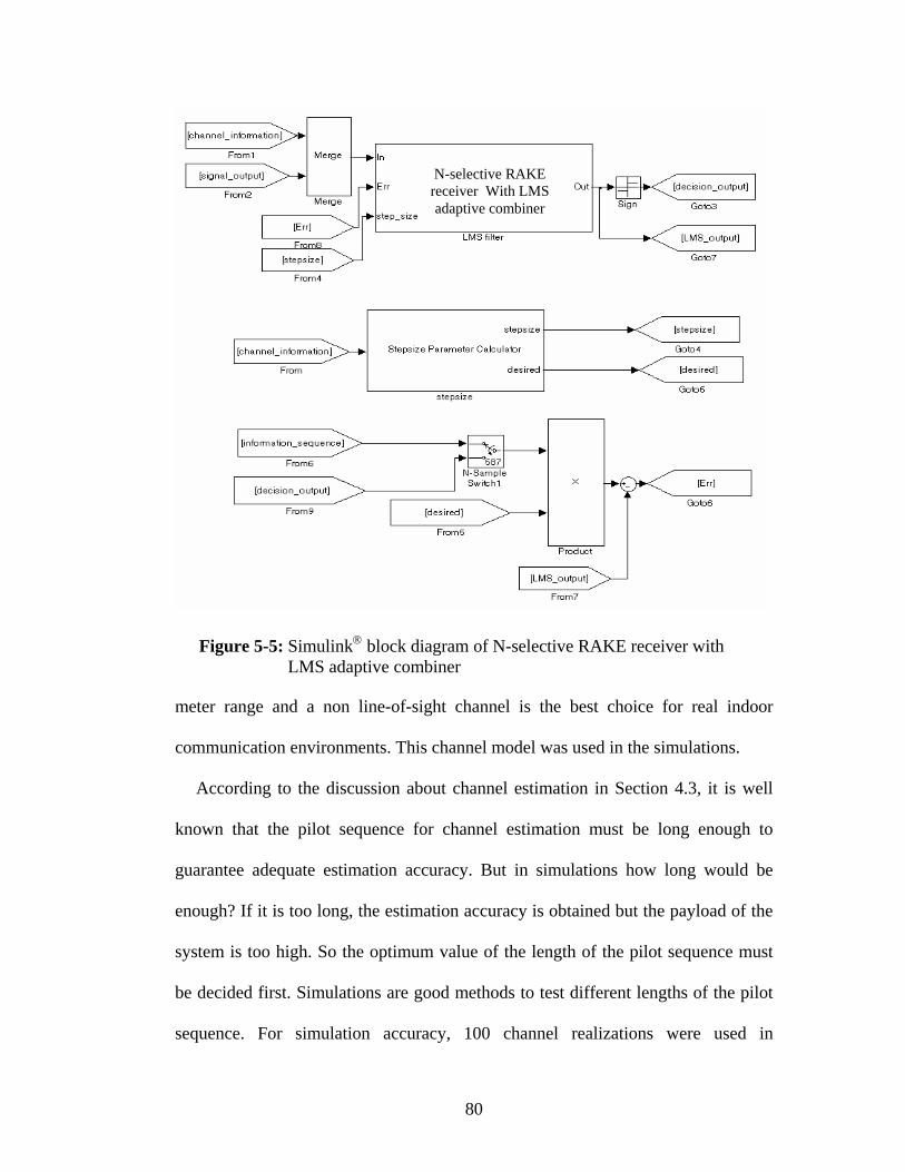
Figure 5-5: Simulink® block diagram of N-selective RAKE receiver with LMS adaptive combiner
N-selective RAKE receiver With LMS adaptive combiner
meter range and a non line-of-sight channel is the best choice for real indoor
communication environments. This channel model was used in the simulations.
According to the discussion about channel estimation in Section 4.3, it is well
known that the pilot sequence for channel estimation must be long enough to
guarantee adequate estimation accuracy. But in simulations how long would be
enough? If it is too long, the estimation accuracy is obtained but the payload of the
system is too high. So the optimum value of the length of the pilot sequence must
be decided first. Simulations are good methods to test different lengths of the pilot
sequence. For simulation accuracy, 100 channel realizations were used in
80

simulation for each length of the pilot sequence and finally an average value of bit
error rate was calculated. The 8-finger MRC RAKE receiver structure was chosen
in simulation. The simulation running time for this sample receiver structure was
short and the optimal length of pilot sequence was decided by channel no matter
what kind of receiver structure was used. Here the binary maximum-length shift-
register pseudo-noise (PN) sequence was used. The lengths were 31, 63, 127 and
255 bits. The Es/N0 level was 10 dB. The result of simulation is shown in Figure 5-
6.
Figure 5-6: The BER for different pilot sequence
From the result it is very clear that between the 31 bits to 127 bits of the pilot
sequence, the BER performance has a sharp increase. After 127 bits the BER
81

performance has almost no improvement as the length of the pilot sequence
increased. Therefore a pilot sequence of 127 bits in length was used.
After the length of pilot sequence was decided, three cases of N-selective MRC
RAKE receiver structures (N= 8, 16, 32) were simulated. The simulation results
and curves fitted to them are shown in Figure 5-7.
Figure 5-7: The BER for N-selective MRC RAKE receiver structures
Before simulating the LMS adaptive equalizer, some parameters must be
obtained. The first one is the number of stages of the LMS equalizer. There still
ought to be an optimum balance between the performance and complexity of the
system. Simulations were used to test the equalizers with different number of
stages. The index for comparing is the system bit error rate. For simulation
82

accuracy, 100 channel realizations were used in simulation for every number of
stages and finally an average value of bit error rate is obtained. The 8-finger MRC
RAKE receiver structure was chosen in this simulation. The Es/N0 level was 20
dB. For low Es/N0 level, the equalizer effect is not obvious. The result of the
simulation is shown in Figure 5-8.
Figure 5-8: The BER for LMS equalizers with different stages
From Figure 5-8 it is very clear that system performance does not always
increase with the number of stages of the LMS equalizer. The LMS equalizer with
11 stages is a reasonable choice for a good balance between performance and
complexity of the system.
83

The second parameter which must be decided before simulating the LMS
adaptive equalizer and the N-selective RAKE receiver with LMS adaptive
combiner is the length of the training sequence. This goal is also pursued by using
simulation. In this simulation the information sequence was used as a training
sequence and the system did not switch to DD mode. The error signal of the LMS
algorithm was recorded. According to the discussion of the LMS algorithm in
Chapter 3, as the LMS algorithm approaches the optimum point step by step, the
error signal decreases continuously and final when arriving optimum point the error
signal will stop to decrease and stay at this value with a small fluctuation. By
observing the error signals the optimum length of training sequence can be
obtained. For the simulation accuracy, 100 simulations for every tap of receiver
structures were run and the final result was the average value. The Es/N0 level was
set at 20 dB.
Based on the results of simulations shown in Figure 5-9 and Figure 5-10, the
length 400 of the training sequence for 8-selective MRC RAKE receiver with LMS
adaptive equalizer and 8-selective RAKE receiver with LMS adaptive combiner
was chosen.
Based on the results of simulations shown in Figure 5-11 and Figure 5-12, the
length 600 of the training sequence for 16-selective MRC RAKE receiver with
LMS adaptive equalizer and 16-selective RAKE receiver with LMS adaptive
combiner was chosen.
Based on the results of simulations shown in Figure 5-13 and Figure 5-14, the
length 800 of the training sequence for 32-selective MRC RAKE receiver with
84

LMS adaptive equalizer and 32-selective RAKE receiver with LMS adaptive
combiner was chosen.
Figure 5-9: The error signal for 8-selective MRC RAKE receiver with LMS adaptive equalizer
Figure 5-10: The error signal for 8-selective RAKE receiver with LMS adaptive combiner
85

Figure 5-11: The error signal for 16-selective MRC RAKE receiver with LMS adaptive equalizer
Figure 5-12: The error signal for 16-selective RAKE receiver with LMS adaptive combiner
86

Figure 5-13: The error signal for 32-selective MRC RAKE receiver with LMS adaptive equalizer
Figure 5-14: The error signal for 32-selective RAKE receiver with LMS adaptive combiner
87

Table 5-1: The Parameters of different receiver structures
Different receiver
structures
8E 8C 16E 16C 32E 32C
Length of pilot sequence
127 127 127 127 127 127
Number of equalizer stages
11 N/A 11 N/A 11 N/A
Length of training sequence
400 400 600 600 800 800
Calculation complexity of processing one information bit
⊗19 ⊕29
⊗8 ⊕16
⊗27 ⊕37
⊗16 ⊕32
⊗43 ⊕53
⊗32 ⊕64
8E: 8-selective RAKE receiver with LMS adaptive equalizer.
8C: 8-selective RAKE receiver with LMS adaptive combiner.
16E: 16-selective RAKE receiver with LMS adaptive equalizer.
16C: 16-selective RAKE receiver with LMS adaptive combiner.
32E: 32-selective RAKE receiver with LMS adaptive equalizer.
32C: 32-selective RAKE receiver with LMS adaptive combiner.
⊗ : multiply operation.
⊕ : add operation.
Like the simulations of the N-selective MRC RAKE receiver structure, three
cases of N-selective MRC RAKE receiver with LMS adaptive equalizer and N-
selective RAKE receiver with LMS adaptive combiner (N= 8, 16, 32) were
simulated.
When the calculation complexity is compared between the N-selective MRC
RAKE receiver with LMS adaptive equalizer and the N-selective RAKE receiver
88

with LMS adaptive combiner, only the different parts will be considered not the
Figure 5-15: The BER for N-selective MRC RAKE receiver with LMS adaptive equalizer
common parts like matched filter, sampling, channel estimation, symbol decision
etc. According to the RAKE MRC combining operation and LMS algorithm
expressed in equations (4.11), (4.13), (4.14) and (4.15), the calculation for
processing one information bit is: N-selective MRC RAKE receiver with LMS
adaptive equalizer include N+11 multiply operations, 1 sum operation of N real
numbers (equally N-1 add operations), 1 sum operation of 11 real numbers (10 add
operations) and 1+11 add operations; N-selective RAKE receiver with LMS
adaptive combiner include N multiply operations, 1 sum operation of N real
89

numbers (N-1 add operations) and 1+N add operations. The summary of parameters
and calculation complexity is listed in Table 4.
The BER simulation results and curves fitted to them are shown in Figure 5-15
and Figure 5-16.
Figure 5-16: The BER for N-selective RAKE receiver with LMS adaptive combiner
5.3 Analysis and discussion
For the three cases of N-selective MRC RAKE receiver structures (N= 8, 16, 32),
the result of the simulation is shown in Figure 5-17. System performance increases
proportionally to N; this coincides with discussions in Chapter 3 on the RAKE
receiver. When N increases, the receiver captures more signal energy leading to the
decrease in BER. In another aspect, it is well known that BER will decrease as the
90
level of SNR or Es/N0 increase. From this simulation result, this is true when
Es/N0 level is less than 20dB. However system performance does not improve
when Es/N0 level is higher than 20dB. This can be explained as follows: The bit
error rate is mainly determined by the ratio of the desired signal energy to the
energy of any other interference signal. When Es/N0 level is less than 20dB, the
main part of the interference signal is from noise signal. When the Es/N0 level
increases, the ratio of the desired signal energy to the energy of any other
interference signal increases leading to the decrease in BER. When the Es/N0 level
is larger than 20dB, a large portion of the interference signal is from ISI. So the
numerator and the denominator of this ratio will increase as Es/N0 level increases
and the result is that this ratio almost has little change. This explanation can also be
demonstrated by the simulation result shown in Figure 5-15 and Figure 5-16
because the N-selective MRC RAKE receiver with LMS adaptive equalizer and the
N-selective RAKE receiver with LMS adaptive combiner both have some
mechanism to suppress the ISI. Another significant outcome is that when the Es/N0
level is lower than 15dB, increasing N does not show an obvious performance
improvement in BER. This exists particularly for 16-selective and 32-selective
MRC RAKE receivers with LMS adaptive equalizer. It is also can be observed that
the cases of N=16 and N=32 looks more promising to combat ISI than the case of
N=8 when Es/N0 level is larger than 15dB. For the simulation result shown in
Figure 5-8, the number of stages of the equalizer is 1 which means the system does
not have an equalizer. The improvement is very obvious when the number of stages
of the equalizer is 11.
91

Figure 5-18: The BER for three different receiver structures with N=16
Figure 5-17: The BER for three different receiver structures with N=8
92

93
From the simulation results shown in Figure 5-17 to Figure 5-19, it is very clear
that both the N-selective MRC RAKE receiver with LMS adaptive equalizer and
the N-selective RAKE receiver with LMS adaptive combiner effectively suppress
ISI and significantly improve system performance.
When either the LMS adaptive equalizer or LMS adaptive combiner is used to
combat ISI, case N=16 obtains higher system performance improvement than the
case N=8. The case N=32 does not obtain obvious system performance
improvement over the case N=16 although the calculation complexity and the
length of training sequence both are increased. The calculation complexity and the
lengths of training sequence of different receiver structures are summarized in
Table 4. For N=16, the LMS adaptive combiner and the LMS adaptive equalizer
Figure 5-19: The BER for three different receiver structures with N=32

both achieved almost same system performances. But the LMS adaptive combiner
has simpler computation complexity. The case N=16 shows the best balance
between performance, computation complexity and length of training sequence.
94

Chapter 6 Conclusions and Future Work
This chapter presents conclusions of the work that was accomplished in this thesis.
e topics for future work to continue the research in this area are also discussed.
.1 Conclusions
ltra wideband (UWB) technology has been proposed recently for use in wireless
ersonal area networks. After gaining regulatory approval, the technology has
oved from academic research topics into the mainstream of telecommunications.
WB is a suitable solution for high speed indoor wireless communications due to
s promising ability to provide high data rate at low cost and low power
onsumption. Another benefit of UWB is its ability to resolve individual multi-path
omponents. This feature motivates the use of RAKE multi-path combining
chniques to provide diversity and capture as much energy as possible of the
ceived signal.
UWB is being considered for use in wireless personal area networks (WPANs),
here the required data rate can be as high as 110 Mbps per user. To obtain such a
te with very low power emission, significant inter-symbol interference (ISI) is
navoidable. Some published results on UWB have neglected this problem as most
erformance analyses employ a RAKE receiver under the assumption that channel
elay spreads are much less than the system symbol time. The traditional RAKE
ceiver structure to collect multi-path energy in UWB systems does not combat ISI
ery well. There is a need to find effective methods to combat ISI.
Som
6
U
p
m
U
it
c
c
te
re
w
ra
u
p
d
re
v
95

I irst
proposal is the N-selective MRC RAKE receiver structure. This is a mixed analog
plexity of the traditional analog RAKE demodulation implementation but also
ampling rate in the digital implementation. A very simple
is equalization algorithm ought to have the ability to track channel
var
e MSE, thereby
n this thesis, three receiver structures were proposed and simulated. The f
and digital implementation. The structure takes advantage of the unique
characteristics of the UWB signal. The structure not only reduces the high
com
avoids the high Nyquist s
and effective channel estimation algorithm (sliding correlation algorithm) is utilized
and integrated into this receiver structure smoothly. From simulation results, this
proposed receiver structure achieved a reasonable BER performance.
The second proposal is the N-selective MRC RAKE receiver with LMS
adaptive equalizer. A LMS adaptive equalizer is added to the N-selective MRC
RAKE receiver with the purpose of suppressing ISI. The channel estimation
outcome provided by the N-selective MRC RAKE receiver is not very accurate. A
fast equalization algorithm is essential in the UWB high speed application
environment. Th
iance. The LMS adaptive equalizer is a good solution for all of these
requirements. From simulation results, this proposed receiver structure indeed
suppresses ISI effectively and exhibits a high BER performance improvement over
the N-selective MRC RAKE receiver.
The third proposal is the N-selective MRC RAKE receiver with LMS adaptive
combiner. The LMS adaptive equalizer and the MRC combiner have similar linear
combing structure. The combination of these two parts, a RAKE combining
structure where the combining weights are chosen to minimize th
96
crea
posed. These
thre
e topics for future research following the
direc
tes a RAKE combining that accomplishes the goals of gathering multi-path
signal energy effectively and suppressing ISI simultaneously. The achievement of
this new idea is demonstrated by simulation results.
From simulation results, the 16-selective MRC RAKE receiver with LMS
adaptive combiner demonstrated the best balance between performance,
computation complexity and length of training sequence among three receiver
structures.
In summary, based on the proposed N-selective MRC RAKE receiver
structures, two new receiver structures for suppressing ISI were pro
e receiver structures were all simulated for N=8, 16 and 32. From simulation
results, ISI is suppressed effectively by these two new schemes. Due to the
simplicity of the algorithm and a 1G Hz sampling rate, the 16-selective MRC
RAKE receiver with LMS adaptive combiner is feasible for practical VLSI
implementations.
6.2 Future work
In this research, many important issues have not been dealt with, or have been
considered with simplified assumptions. Hence, there are some areas in which the
work of this thesis can be extended. Som
tion of this thesis are issued here:
• The inter-pulse interference was neglected in the theory derivation in Chapter 4
and was not considered in this thesis. The methods for suppressing this
interference could be studied. The scheme of using signal processing technologies
97
or designing pulse shape with better inter-pulse interference immunity properties
could be considered.
• The UWB channel model is a static model and its parameters do not change
d
ul for the future hardware implementation.
• O
uring simulations. Adding some time-variant properties to the channel model
and making it more close to the realistic indoor channel could be considered
• Constructing a hardware test-bed to verify the simulation is also very important
and helpf
ther adaptive filter algorithms could be considered instead of the LMS algorithm
used in this thesis. System performance, computation complexity and difficulty of
implementation could be analyzed.
98

Bibliography
] T. W. Barrett, “History of Ultra Wide Band (UWB) Radar & Communications
ioneers and Innovators,” In Proc. Progress In Electromagnetic Symposium 2
[1
P 000
[2 unications,” Multi-Spectral
[3
P s Regarding Ultra-Wideband Transmission
ystems,” ET Docket 98-153, Feb. 14, 2002.
] J. Foerster et al., “Channel modeling sub-committee report final,” IEEE P802.15
ireless Personal Area Networks, P802.15-02/490r1-SG3a, Feb. 2003.
] J. D. Choi and W.E. Stark, “Performance of Ultra-Wideband Communications
ith Suboptimal Receivers in Multi-path Channels,” IEEE Journal on Selected
reas in Communications, vol. 20, pp. 1754-1766, Dec. 2002.
] M. Z. Win and R.A. Scholtz, “Ultra-wide bandwidth time-hopping spread-
ectrum impulse radio for wireless multiple-access communications,” IEEE Trans.
ommun., vol. 48, pp. 679–689, Apr., 2000.
] Multi-Band OFDM Alliance, “Ultra wideband: High-speed, short-range
chnology with far-reaching effects,” MBOA-SIG White Paper, September, 2004,
ttp://www.multibandofdm.org/papers/MBOA_UWB_White_Paper.pdf
(PIERS2000), Cambridge, MA, July, 2000.
] R. J. Fontana, “A Brief History of UWB Comm
Solutions Inc..
] Federal Communications Commission, “First Report and Order, Revision of
art 15 of the Commission’s Rule
S
[4
W
[5
w
A
[6
sp
C
[7
te
h .
99

[8] R. T. Hoctor and H. W. ed transmitted reference RF
communications,” Proc. 2002 UWBST, pp. 265-270, May 2002.
] A Saleh and R. Valenzuela, “A statistical model for indoor multi-path
f ultra-wide bandwidth wireless indoor
s, vol. 20, no. 9, pp. 1613-1627, Dec. 2002.
d fading on the performance of direct
tt., vol. 2, pp. 245–
n Selected Areas in Communications,
A Indoor
Tomlinson, “Delay-hopp
[9
propagation,” IEEE Journal on Selected Areas in Communications, vol. 5, pp. 128-
137, Feb. 1987.
[10] M. Win, R. Scholtz, “Characterization o
channels: a communication-theoretic view,” IEEE Journal on Selected Areas in
Communication
[11] R. Price, P. E. Green, “A Communication Technique for Multi-path
Channels,” Proc. IRE., vol. 46, pp. 555-570, Mar. 1958.
[12] G. L. Turin, “The effect of multipath an
sequence CDMA systems,” IEEE Journal on Selected Areas in Communications,
vol. 2, pp. 597-603, Jul. 1994.
[13] J. G. Proakis, Digital Communications, 4th edition, McGraw Hill Inc., 2001.
[14] M. Z. Win and R. A. Sholtz, “On the energy capture of ultrawide bandwidth
signals in dense multipath environments,” IEEE Commun. Le
247, Sep. 1998.
[15] V. Lottici, A. D’Andrea, and U. Mengali, “Channel estimation for ultra-
wideband communications,” IEEE Journal o
vol. 20, no. 9, pp. 1638–1645, 2002.
[16] R. Fantacci and A. Galligani, “An Efficient RAKE Receiver Architecture with
Pilot Signal Cancellation for Downlink Communications in DS-CDM
100

Wireless Networks,” IEEE Transactions on Communications, vol. 47, no. 6, June
1999, pp. 823-827.
[17] A. J. Viterbi, CDMA, Principles of Spread Spectrum Communication. Reading,
MA: Addison Wesley, 1995.
[18] T. S. Rappaport, Wireless Communications. Upper Saddle River, NJ: Prentice
ol. 3, pp. 308–310, Nov.
ain,” in Proc. IEEE Conf. Ultra Wideband Systems
s, New Jersey 07632, first edition, 1995.
Finland, June 2001, pp. 2948–2952.
1186–1196, June 2001.
Hall, 1996.
[19] Brennan, D. G. “Linear Diversity Combining Techniques,” Proc. IRE., vol. 47,
pp. 1075-1102.
[20] M. Z. Win and Z. A. Kostic´, “Virtual path analysis of selective Rake receiver
in dense multipath channels,” IEEE Commun. Lett., v
1999.
[21] J. Keignart and N. Daniele, “Subnanosecond UWB Channel Sounding in
Frequency and Temporal Dom
and Technol., pp. 25-30, May 2002.
[22] Marvin K. Simon, Sami M. Hinedi, and William C. Lindsey, Digital
Communication Techniques: Signal Design and Detection, Prentice Hall,
Englewood Cliff
[23] L. Zhao and A. M. Haimovich, “Performance of ultra-wideband
communications in the presence of interference,” in Proc. IEEE Int. Conf.
Communications (ICC’01), Helsinki,
[24] F. Ramirez-Mireles, “Performance of ultra wideband SSMA using
timehopping And M-Ary PPM,” IEEE J. Select. Areas Commun., vol. 19, pp.
101

[25] Rusch, L. A., C. Prettie, D. Cheung, Q. Li, and M. Ho, "Characterization of
UWB Propagation from 2 to 8 GHz in a Residential Environment," IEEE Journal
aptive interference suppression for direct-sequence
z-Mireles, F., "On the performance of ultra-wideband signals in
. 244-249, Jan 2001 .
. Cassioli, M. Z. Win, A. F. Molisch, and F. Vatelaro, “Performance of
l, “A comparison between ultra wideband and
chnology: Potential and
on Selected Areas in Communications, submitted December 2001.
[26] Madhow, U., "Blind ad
CDMA," Proceedings of the IEEE , vol. 86, no. 10, pp. 2049-2069, Oct. 1998.
[27] Ramire
gaussian noise and dense multipath," IEEE Transactions on Vehicular Technology,
vol. 50, no. 1, pp
[28] M. Z. Win and R. A. Scholtz, “Impulse radio: How it works,” IEEE Comm.
Lett., vol. 2, pp. 36–38, Feb 1998.
[29] D
selective Rake reception in a realistic UWB channel,” in Proc. ICC 2002, pp. 763–
767, 2002.
[30] D. Barras, F. Ellinger, H. Jacke
narrowband transceivers,”
http://www.ife.ee.ethz.ch/~ellinger/Homepage/UWB2002.pdf
[31] D. Porcino, W. Hirt, “Ultra-Wideband Radio Te
Challenges Ahead,” IEEE Communications Magazines, pp. 66-74, July 2003.
[32] Simon Haykin, Adaptive Filter Theory, 4th edition, Prentice Hall Inc., 2001.
102

Appendix A: Discrete-time model for a channel
with ISI
The received base-band signal can be expressed as
+−= ∑ (A.1)
represents the additive white Gaussian
)()()( tznTthItrn
nl
where { }nI is the information sequence, )(th represents the response of the channel
to the input signal pulse )(tg and z )(t
noise. Since the transmitter sends discrete-time symbols at a rate of T1 symbols/s
and the sampled output of the matched filter at the receiver is also a discrete-time
T1 per second, the cascade of the analog signal with samples occurring at a rate of
filter at th transmitte pulse response , the channel with impulse
response ) , the matched filter at the receiver with impulse response , and
an equivalent discrete-time transversal filter
e r with im )(tg
(tc )( th −∗
the sampler can be represented by
having tap gain coefficients { }kx . This equivalent discrete-time transversal filter
spans a time interval of LT2 seconds. Its input is the sequence of information
symbols { }kI and its output is the discrete-time sequence { }ky given by Eq.A.1.
2)
here (A.3)
(A.4)
knknk xIy υ+= ∑ − (A.n
dtkTthtrkTyy lk ∫∞
∞−
∗ −=≡ )()()(W
dtkTththkTxxk ∫∞
∞−
∗ +=≡ )()()(
denotes the additive noise sequence at the output of the matched filter, kυ
103
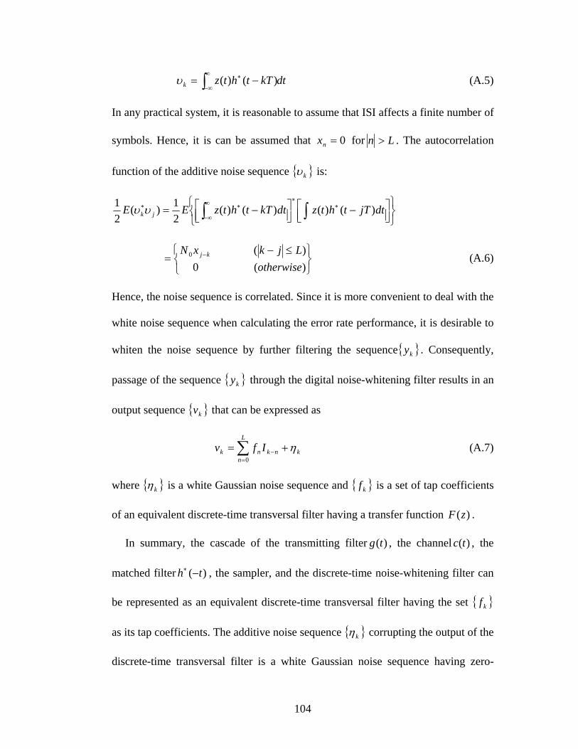
dtkTthtzk ∫∞
∞−
∗ −= )()(υ (A.5)
able to assume that ISIn any practical system, it is reason I affects a finite number of
mbols. Hence, it is can be assumed that 0=nx for Ln > . The autocorrelation sy
function of the additive noise sequence { }kυ is:
⎭⎬⎫
⎩⎨⎧
⎥⎦⎤
⎢⎣⎡ −⎥⎦
⎤⎢⎣⎡ −= ∫∫ ∗
∗∞
∞−
∗∗ dtjTthtzdtkTthtzEE jk )()()()(21)(
21 υυ
⎭⎬
⎩⎨=
−
)(00
otherwkj (A.6)
Hence, the noise sequence is correlated. Since it is more convenient to deal with the
white noise sequence when calculating the error rate performance, it is desirable to
whiten the noise sequence by further fil ng the sequence
⎫⎧ ≤− )(ise
LjkxN
teri { }ky . Consequently,
passage of the sequence { }y through the digital noise-whitening filter results in an
output sequence { }v that can be expressed as
k
L
nnkk
k
k
n Ifv η+= ∑=
(A.7) −0
where { }kη is a white Gaussian noise sequence and { }kf is a set of tap coefficients
of an equivalent discrete-time transversal filter having a transfer function )(zF .
In summary, the cascade of th
matched filter , the sampler, and the discrete-time noise-white
be represented as an equivalent discrete-time transversal filter having the set
e transmitting filter )(tg , the channel )(tc , the
)( th −∗ ning filter can
{ }kf
as its tap coefficients. The additive noise sequence { }kη corrupting the output of the
dis ng zero-crete-time transversal filter is a white Gaussian noise sequence havi
104

mean and variance . Figure A-1 illu
0N strates the discrete-time model for a channel
with ISI.
1−z 1−z 1−z{ }kI
1−z
0f 1f 1−Lf Lf
{ }kη
{ }kv 1−z =delay of T
Figure A-1: Equivalent discrete-time model of ISI channel with AWGN
105
Appendix B: Zero-forcing equalizer
Eq.A.7 is rewritten here.
(B.1)
The linear equalization process can be expressed as
(B.2)
where
k
L
nnknk Ifv η+= ∑
=−
0
∑∞
−∞=−=
jjkjk vcI
{ }jc are the complex-valued tap weight coefficients of the linear equalizer.
Sequence is the demodulator output and sequence { }kv { }kI is the estimate of the
information sequence . The equalizer is assumed to have an infinite number of
taps.
It is observed that the cascade of the discrete-time linear filter model having an
pulse response and an equalizer having an impulse response can be
presented by a single equivalent filter having the impulse response
(B.3)
is simply the convolution of
{ }kI
{ }nf { }ncim
re
∑∞
−∞=−=
jjnjn fcq
{ }nq { }nc and { }nf . Its output at the kth sampling
stant can be expressed in the form
(B.4)
in
∑∑∞
−∞=−
≠− ++=
jjkj
knnknkk cqIIqI η0
ˆ
106

The first bol. The
second term is the inter-symbol interference. The peak value of this interference,
term in Eq.B.3 represents a scaled version of the desired sym
which is called peak distortion, is
∑≠
=0
)(n
nqcD
∑ ∑≠ −∞=
−0n j
jnj
∞
= fc (B.5)
Where is a function of the e
With an equalizer having an infinite number of taps, it is possible to select the tap
)(cD qualizer tap coefficients.
weights so that 0)( =cD , i.e., 0=nq for all n except 0=n . That is, the inter-
symbol interference can be completely eliminated. The values of the tap weights to
accomplish this goal are determined from the condition
⎭
By taking the z transform of Eq.B-5, it is obtained
⎬⎫
⎩⎨⎧
≠=
== ∑∞
−∞=− )0(0
)0(1nn
fcqj
jnjn (B.6)
1)()()( == zFzCzQ (B.7)
)(1)(zF
zC = (B.8)
where ) denotes the transform of the (zC z { }jc . Note that the equalizer, with
transfer function , is simply the inverse filter to the linear filter model . In
other words, complete elimination of the inter-symbol interference requir use
of an inverse filter to . Such equalizer is called
)(zC )(zF
es the
)(zF a zero-forcing equalizer.
107

Appendix C: Mean-square-error (MSE)
criterion linear equalizer
In the MSE criterion, the tap weight coefficients { }jc of the equalizer are adjusted
to minimize the mean square value of the error
22 ˆkkk IIEEJ −== ε (C.1)
f that sy t the o th er. H
“The necessary and sufficient condition for the cost function to obtain its
minimum value is for the corresponding value of the estima
where kI is the information symbol transmitted in the kth signaling interval and kI
is the estimate o mbol a utput of e equaliz ere the principle of
orthogonality, one of the most elegant theorems in the subject of linear optimum
filtering, was stated:
J
tion error kε to be
the estimation of the desired
response at time .”
When the equalizer is
equalization process can be expressed as
orthogonal to each input sample that enters into
k
assumed to have a finite number of taps, the linear
∑ −=K
−=k vcI (C.2)
Kjjkj
where { }jc are the complex-valued tap weight coefficients of the linear equalizer.
Sequence { }kv is the demodulator output. For the cost function J to obtain its
inimum value, the orthogonal condition which must be satisfied is expressed as: m
( ) KlKvE lkk <<−=∗− ,0ε (C.3)
108

tution for kε in Eq.C.3 yields
0=⎥⎤
⎟⎟⎞
− ∗−−∑ lk
K
jkjk vvcI
Substi
⎥⎦⎢⎢⎣
⎡
⎠⎜⎜⎝
⎛
−= KjE (C.4)
equivalently,
K
<<−∗∗ (C.5)
It is convenient to express the set of linea
(C.6)
Let denote the (2K+1)-by-(2K+1) correlation matrix of the demodulator output
v :
( ) ( ) KlKvIEvvEc lkkKj
lkjkj = −−=
−−∑ ,
r equations in matrix form. Thus,
Ρ=ΓC
Γ
sequence{ }k
[ ])()( kVkVE=Γ T∗ (C.7)
W
o ut uenc
here [ ]TKkKkkKkKk vvvvvkV +−+−−−= ,,,,,,)( )1()1( KK is the (2k+1)-by-1 demodulator
output sequence{ }kv vector at time k.
Correspondingly, let Ρ denote the (2k+1)-by-1 cross-correlation vector between
the demodulator utp seq e{ }kv vector and the information signal kI :
[ ]kIkVE )(∗=Ρ (C.8)
[ ]TKKKK cccccC −−−−= ,,,,,, )1(01 KK is the (2k+1)-by-1 equalizer coefficients vector.
The solution of Eq.C.6 is
ΡΓ= −1optimumC (C.9)
where 1−Γ is the inverse matrix of Γ .
109

Appendix D: Proced ure to calculate a gradient
vect
Gradient vector of a cost function
or
)(wJ r )(wJ r∇, which is denoted by , is written.
⎥⎥⎥
⎢⎢
∂∂ wJwJ )()( rr M⎥⎥
⎢⎢
∂∂
+∂∂
= bwJj
awJ )()( ⎥
⎦⎢
⎢
⎣ ∂+
∂
∂∂
∂∂
=∇
MM bj
a
wJwJ
wwJwJ
)()(
)()(22
11 rr⎥⎤
⎢⎡
∂+
∂ bj
a
r r
r
rr
where jbajbaw
(D.1)
[ ]MM jba +++= ,, 2211 L ,r is a complex valued vector.
The linear equalization pro
∑
cess can be expressed as
−=kjv (D.2)
wh
−=Kj
jk cI K
ere { } { }jjj jbac += are the complex-valued tap weight coefficients of the linear
equalizer. Sequence { }is the dem ator output. kv odul
The cost function is J
22 ˆkkk IIEEJ −== ε
[ ] [ ]∗∗ −−== )ˆ)(ˆ( kkkkkk IIIIEE εε
substituting Eq.D.2.
[ ] [ ] [ ] [ ]∑ ∑∑∑−= −=
∗−−
∗
−=−−
−=
∗ +−−=K
Kj
K
Kiikjkij
KK
Kjkjkjkjk
Kjjk vvEccIvEcIvEcIE **2 (D.3)
110

The gradient vector of the cost function J based on the equalizer coefficients
vector is [ ]TKKKK cccccC −−−−= ,,,,,, )1(01 KK
[ ]( ) [ ] [ ]C
IvEc
C
IvEc
CIE
CCJCJ
K
Kjkjkjkjk
K
Kjj
k
∂
⎟⎟⎠
⎞⎜⎜⎝
⎛∂
−∂
⎟⎟⎠
⎞⎜⎜⎝
⎛∂
−∂
∂=
∂∂
=∑∑−=
−−−=
∗ **2
)()( ∇
[ ]C
vvEccK
Kj
K
Kiikjkij
∂
⎟⎟⎠
⎞⎜⎜⎝
⎛∂
+∑ ∑−= −=
∗−−
∗
(D.4)
Now the four parts on the right-hand side w
1. for the first part,
ill be calculated separately:
[ ]( )
⎥⎦
⎢⎣0⎥⎥⎥⎤
⎢⎢⎢⎡
=∂
00
2
MCIk is a (2k+1)-by-1 null vector.
2. for the second part,
∂ E
[ ]
[ ] [ ]
[ ] [ ]
[ ] [ ]⎥⎥⎥⎥⎥⎥⎥⎥⎥⎥⎥
⎦
⎤
⎢⎢⎢⎢⎢
⎢
⎢⎢⎢
⎣
⎡
∂
⎟⎟⎠
⎞⎜⎜⎝
⎛∂
+∂
⎟⎟⎠
⎞⎜⎜⎝
⎛∂
∂
⎟⎟⎠
⎞⎜⎝+
∂
⎟⎠
⎜⎜⎝
⎛∂
∂
⎟⎞
⎜⎛
∂
⎟⎞
⎜⎛∂
=⎠⎝
−
−−=
∗
−
−−=
∗
−
−−=
−
−−=
∗∗
−=
∑
∑
K
kjk
K
Kjj
K
kjk
K
Kjj
K
kjkKj
j
K
kjkKj
j
K
K
K
K
Kj
b
IvEcj
a
IvEc
b
Ivj
a
ba
**
1
*
1
**
M
⎥⎥
⎢⎢
⎜⎛∂⎟
⎞
⎟⎠
⎜⎝∂
+⎟⎠
⎜⎝
⎟⎟⎞
⎜⎜⎛∂ ∗∗
−−=
−−=
−∗
∑
∑∑
∑ KK
kjkKj
jkjkKj
j
kjk
K
j EcIvEc
IvEcj
IvEc
IvEc **
⎢⎢∂C
∑
111

[ ]( ) [ ]( )
[ ]( ) [ ]( )
[ ]( ) [ ]( )⎥⎥⎥⎥⎥⎥⎥⎥
⎦⎢⎢⎢⎢⎢⎢⎢⎢
⎣ ∂∂
+∂
∂
∂+
∂
∂∂
+∂
=
−
+∗−
−
+∗−
−
−−∗−
−
−−∗−
K
kKkK
K
kKkK
K
kKkK
K
kKkK
KK
bIvEc
ja
IvEc
bIvEc
ja
IvEcb
cj
a
**
1
*)1(1
1
*)1(1
M
⎤⎡
∂
∂∂ −∗
−∗
kKkKkKkK IvEIvEc **
( ) [ ]( ) ( ) [ ]( )
( ) [ ]( ) ( ) [ ]( )
( ) [ ]( ) ( ) [ ]( )⎥⎥⎥⎥⎥
⎥
⎦
⎤
⎢⎢⎢⎢⎢⎡
∂+
∂
∂+
∂
−∂∂
−∂+
∂−∂
=
−
+−−
−
+−−
−−
−−−−
−−
K
kKkKK
K
kKkKK
KK
kKkKK
kKkKK
K
kKkKK
bj
a
bj
aIvEjba
bIvEjba
ja
IvEjba
11
*)1(11
**
⎥⎥
−∂ −−−− kKkKK
K
IvEjba *)1(11
⎢⎣
⎢⎢
−∂−∂ IvEjbaIvEjba **M
[ ] ( ) [ ][ ]
( ) ]
[ ] ( ) [ ] ⎥⎥⎥⎥⎥
⎦
⎤
⎢⎢⎢
⎣
⎡
−+
−+
=
++
−
−−
kKkkKk
k
kKkkKk
IvEjjIvE
IIvEjjIvE
**
)1
**
M
3. for the third part,
[⎢⎢ −+ −−− KkkKk vEjjIvE *
(*
)1(
[ ][ ]
[ ] ⎥⎥⎥⎥⎥
⎦
⎤
⎢⎢⎢⎢⎢
⎣
⎡
=
+
−−
−
kKk
kKk
kKk
IvE
IvEIvE
*
*)1(
*
2M
[ ]
[ ] [ ]
[ ] [ ]
[ ] [ ]⎥⎥⎥⎥⎥⎥⎥⎥⎥⎥⎥⎥⎥
⎦
⎤
⎢⎢⎢⎢⎢⎢⎢⎢⎢⎢⎢⎢⎢
⎣
⎡
∂
⎟⎟⎠
⎞⎜⎜⎝
⎛∂
+∂
⎟⎟⎠
⎞⎜⎜⎝
⎛∂
∂
⎟⎟⎠
⎞⎜⎜⎝
⎛∂
+∂
⎟⎟⎠
⎞⎜⎜⎝
⎛∂
∂
⎟⎟⎠
⎞⎜⎜⎝
⎛∂
+∂
⎟⎟⎠
⎞⎜⎜⎝
⎛∂
=∂
⎟⎟⎠
⎞⎜⎜⎝
⎛∂
−
∗−
−=
−
∗−
−=
−
∗−
−=
−
∗−
−=
∗−
−=
∗−
−=
∗−
−=
∑∑
∑∑
∑∑
∑
K
kjk
K
Kjj
K
kjk
K
Kjj
K
kjk
K
Kjj
K
kjk
K
Kjj
K
kjk
K
Kjj
K
kjk
K
Kjj
kjk
K
Kjj
b
IvEcj
a
IvEc
b
IvEcj
a
IvEc
b
IvEcj
a
IvEc
C
IvEc
M11
112

[ ]( ) [ ]( )
[ ]( ) [ ]( )
[ ]( ) [ ]( )⎥⎥⎥⎥⎥⎥⎥⎥
⎦
⎤
⎢⎢⎢⎢⎢⎢⎢⎢
⎣
⎡
∂∂
+∂
∂
∂
∂+
∂
∂∂
∂+
∂∂
=
−
∗+−
−
∗+−
−
∗−−−
−
∗−−−
∗−
∗−
K
kKkK
K
kKkK
K
kKkK
K
kKkK
K
kKkK
K
kKkK
bIvEc
ja
IvEc
bIvEc
ja
IvEcb
IvEcj
aIvEc
M1
)1(1
1
)1(1
( ) [ ]( ) ( ) [ ]( )
( ) [ ]( ) ( ) [ ]( )
( ) [ ]( ) ( ) [ ]( )⎥⎥⎥⎥⎥⎥⎥⎥
⎦
⎤
⎢⎢⎢⎢⎢⎢⎢⎢
⎣
⎡
∂+∂
+∂
+∂
∂
+∂+
∂
+∂∂
+∂+
∂+∂
=
−
∗+−−
−
∗+−−
−
∗−−−−
−
∗−−−−
∗−
∗−
K
kKkKK
K
kKkKK
K
kKkKK
K
kKkKK
K
kKkKK
K
kKkKK
bIvEjba
ja
IvEjba
bIvEjba
ja
IvEjbab
IvEjbaj
aIvEjba
M1
)1(11
1
)1(11
[ ] ( ) [ ][ ] ( ) [ ]
[ ] ( ) [ ] ⎥⎥⎥⎥⎥
⎦
⎤
⎢⎢⎢⎢⎢
⎣
⎡
+
++
=
∗+
∗+
∗−−
∗−−
∗−
∗−
kKkkKk
kKkkKk
kKkkKk
IvEjjIvE
IvEjjIvEIvEjjIvE
M)1()1(
⎥⎥⎥⎥
⎦
⎤
⎢⎢⎢⎢
⎣
⎡
=
0
00
M is a (2k+1)-by-1 null vector.
4. for the fourth part,
[ ]
[ ] [ ]
[ ] [ ]
[ ] [ ]⎥⎥⎥⎥⎥⎥⎥⎥⎥⎥⎥⎥⎥
⎦
⎤
⎢⎢⎢⎢⎢⎢⎢⎢⎢⎢⎢⎢⎢
⎣
⎡
∂
⎟⎟⎠
⎞⎜⎜⎝
⎛∂
+∂
⎟⎟⎠
⎞⎜⎜⎝
⎛∂
∂
⎟⎟⎠
⎞⎜⎜⎝
⎛∂
+∂
⎟⎟⎠
⎞⎜⎜⎝
⎛∂
∂
⎟⎟⎠
⎞⎜⎜⎝
⎛∂
+∂
⎟⎟⎠
⎞⎜⎜⎝
⎛∂
=∂
⎟⎟⎠
⎞⎜⎜⎝
⎛∂
−
−= −=
∗−−
∗
−
−= −=
∗−−
∗
−
−= −=
∗−−
∗
−
−= −=
∗−−
∗
−= −=
∗−−
∗
−= −=
∗−−
∗
−= −=
∗−−
∗
∑ ∑∑ ∑
∑ ∑∑ ∑
∑ ∑∑ ∑
∑ ∑
K
K
Kj
K
Kiikjkij
K
K
Kj
K
Kiikjkij
K
K
Kj
K
Kiikjkij
K
K
Kj
K
Kiikjkij
K
K
Kj
K
Kiikjkij
K
K
Kj
K
Kiikjkij
K
Kj
K
Kiikjkij
b
vvEccj
a
vvEcc
b
vvEccj
a
vvEcc
b
vvEccj
a
vvEcc
C
vvEcc
M11
113

[ ] [ ] [ ]
[ ] [ ] [ ]
[ ] [ ] [ ]⎥⎥⎥⎥⎥⎥⎥⎥⎥⎥⎥⎥⎥⎥⎥⎥⎥
⎦
⎤
⎢⎢
⎜⎝ −≠ Ki
K⎢⎢⎢⎢⎢⎢⎢⎢⎢⎢
⎢⎢⎢
⎣
⎡
∂Ψ
+∂
⎟⎟⎠
⎞⎜⎛
++∂
∂Ψ
+∂
⎟⎟⎠
⎞⎜⎜⎝
⎛++∂
∂Ψ
+∂
⎟⎟⎠
⎞⎜⎜⎝
⎛++∂
=
−
−
−
Ψ
∗++
∗−−
−≠
∗+−
∗−
∗−+
∗−
−
−
−
Ψ
∗−−−−
∗−−
−≠ −≠
∗−−−
∗−
∗−−−
∗−
Ψ
∗−−
∗
≠ ≠
∗−−
∗∗−−
∗
−
−
∑ ∑
∑ ∑
∑ ∑
K
K
K
KkKkKKKj
KkjkjKikKki
K
K
K
KkKkKKKi Kj
KkjkjKikKkiK
K
K
K
KkKkKKKi Kj
KkjkjKikKkiK
bj
a
vvEccvvEccvvEcc
bj
a
vvEccvvEccvvEcc
bj
a
vvEccvvEccvvEcc
K
K
K
444444444444 8444444444444 76M
444444444444444 8444444444444444 76
44444444444 844444444444 76
1
1
1
)1()1(111 1
)1(1)1(1
1
⎢⎢
[ ] [ ] [ ]
[ ] [ ] [ ]
[ ] [ ] [ ]⎥⎥⎥⎥⎥⎥⎥⎥
⎦
⎤
⎢⎢⎢⎢
=−≠
−Kj
kjkj1
⎢⎢⎢⎢
⎣
⎡
∂+
+∂
++
∂+
+∂
++
∂+
+∂
++
−
∗++−−
−
∗++−−
−≠
∗+−
−
∗−−−−−−
−
∗−−−−−−∗
−−
∗−−
∗−−
≠
∗−−
∑
∑
∑
K
KkKkKK
K
KkKkKK
KjKkjkj
K
KkKkKK
K
KkKkKKK
K
KkKkKK
K
KkKkKK
KjKkjkj
bvvEbaj
avvEbavvEc
bvvEba
ja
vvEbavvEc
bvvEbaj
avvEbavvEc
)()(2
)()(2
)()(2
2222
1
)1()1(2
12
1
1
)1()1(2
12
1)1(
2222
M
⎥
[ ]⎥⎥
⎢⎢ ∑
−=−
Kjjkj vvEc
[ ]
[ ] ⎥⎥⎥⎥⎥
⎦
⎤
⎢
⎢⎢⎢
⎣
⎡
= ∑
−=+−
−=
∗−−−
∗−
KjKkjkj
K
KjKkjkj
K
Kk
vvEc )1(2
The gradient vector of the cost function based on the equalizer coefficients
vector can be rewritten
(D.5)
⎢⎢∑ ∗
K
vvEcM
J
[ ]TKKKK cccccC −−−−= ,,,,,, )1(01 KK
[ ][ ]
[ ]
[ ]
[ ]
[ ]
C
vvEc
vvEc
vvEc
IvE
IvEIvE
CJ
K
KjKkjkj
K
KjKkjkj
K
KjKkjkj
kKk
kKk
kKk
Γ+Ρ−=
⎥⎥⎥⎥⎥⎥⎥⎥
⎦
⎤
⎢⎢⎢⎢⎢⎢⎢⎢
⎣
⎡
+
⎥⎥⎥⎥⎥
⎦
⎤
⎢⎢⎢⎢⎢
⎣
⎡
−=∇
∑
∑
∑
−=
∗+−
−=
∗−−−
−=
∗−−
+
−−
−
2222)( )1(
*
*)1(
*
MM
114

Let denote the (2K+1)-by-(2K+1) correlation matrix of the demodulator output Γ
sequence{ }kv :
[ ])()( kVkVE T∗=Γ
where is the (2k+1)-by-1 demodulator
Correspondingly, let denote the (2k+1)-by-1 cross-correlation vector between the
demodulator output sequence
[ ]TKkKkkKkKk vvvvvkV +−+−−−= ,,,,,,)( )1()1( KK
output sequence{ }kv vector at time k.
Ρ
{ }kv vector and the information signal : kI
[ ]kIkVE )(∗=Ρ
[ ]TKKKK cccccC −−−−= ,,,,,, )1(01 KK is the (2k+1)-by-1 equalizer coefficients vector.
115


![[PPT]Floating Point Analysis - Πανεπιστήμιο Ιωαννίνωνvoippimrc08/present/VoIP_3GPP.ppt · Web viewBoth Rake and Equalizer w/ and w/o receiver diversity at the](https://img.pdfslide.net/doc/110x75/5ae9813b7f8b9a8b2b914dd1/pptfloating-point-analysis-voippimrc08presentvoip3gpppptweb.jpg)


![Comparative Performance Analysis of G-RAKE … · Comparative Performance Analysis of G-RAKE Receivers with Suboptimal Finger ... An attractive choice is the RAKE receiver [6]](https://img.pdfslide.net/doc/110x75/5b2021237f8b9a45458b4a1d/comparative-performance-analysis-of-g-rake-comparative-performance-analysis.jpg)