Journal of Operation and Automation in Power Engineering

Vol. 7, No. 1, May 2019, Pages: 65 - 77

http://joape.uma.ac.ir

Adaptive Sliding Mode Control of a Multi-DG, Multi-Bus Grid-Connected

Microgrid.

F. Shavakhi Zavareh 1, E. Rokrok 1, *, J. Soltani 2, 3 , M.R. Shakarami1

1 Department of Technical & Engineering, Lorestan University, Khorramabad, Iran. 2 Department of Electrical Engineering, Khomeinishahr Branch, Islamic Azad University, Isfahan, Iran.

3 Faculty of Electrical and Computer Engineering, Isfahan University of Technology.

Abstract- This paper proposes a new adaptive controller for the robust control of a grid-connected multi-DG microgrid

(MG) with the main aim of output active power and reactive power regulation as well as busbar voltage regulation of

DGs. In addition, this paper proposes a simple systematic method for the dynamic analysis including the shunt and

series faults that are assumed to occur in the MG. The presented approach is based on the application of the slowly

time-variant or quasi-steady-state sequence networks of the MG. At each time step, the connections among the MG

and DGs are shown by injecting positive and negative current sources obtained by controlling the DGs upon the sliding

mode control in the normal and abnormal operating conditions of the MG. Performance of the proposed adaptive sliding mode controller (ASMC) is compared to that of a proportional-integral (PI)-based power controller and SMC

current controller. The validation and effectiveness of the presented method are supported by simulation results in

MATLAB-Simulink.

Keyword: Adaptive sliding mode control, Dynamic analysis, Distributed generation, Microgrid, Unsymmetrical.

Fault.

1. INTRODUCTION

A microgrid (MG) consists of a group of loads and

distributed energy resources (DERs), such as distributed

generations (DGs), battery energy storage systems

(BESSs), photovoltaic cells, diesel engines, wind energy

conversion systems, and fuel cells. An MG has the ability

to operate grid-connected and islanded modes and

manage the transitions between these two modes [1-2]. In

the grid-connected mode, the main grid can provide the

power shortage of the MG, and the additional power

generated in the MG can be exchanged with the main

grid. In the islanded mode, the real and reactive power

generated by DGs should be in balance with the demand

for local loads in Ref. [3]. Recently, MG analysis has

become important due to the expansion of the MG system

and automation of its operation. There are , however,

certain operational challenges in the design of MG

control and protection systems such as reliability

assessment, energy management system, stability issues,

and power quality. One of the characteristics of smart

grids is uncertain generation and load profiles which have

to be considered in evaluating the reliability of the MGs.

In Ref. [4], the normal distribution function is used for

representing uncertainties involved in both DG units and

load demand within an MG. Moreover, in Ref. [5]

employs an incentive-based demand response program

and examines its effects on the MG energy management

system problem. The objective functions of the MG

energy management system problem include total cost

and emission. The main control variables for the MG

control are voltage, frequency, and active and reactive

power; in the grid-connected mode, the frequency and

the voltage at the PCC are dominantly determined by the

main grid in Ref. [3]. With respect to the control of DGs

and the analysis of inverter-based MGs under unbalanced

load and external fault conditions, the employment of

appropriate power, current, and voltage control strategies

is very important for enhancing power quality [6-10].

Some possible control strategies that distributed power

generation systems can use under grid disturbances in the

MG are discussed in Ref. [6]. This paper provides

strategies for generating current references, and

analytical equations are provided and discussed.

Received: 28 May. 2018

Revised: 17 Agust 2018 and 10 October 2018

Accepted: 00 Mar. 00 Corresponding author:

E-mail: rokrok.e@lu.ac.ir (E. Rokrok)

Digital object identifier: 10.22098/joape.2019.4843.1371

Research Paper

2019 University of Mohaghegh Ardabili. All rights reserved.

F. Shavakhi Zavareh, E. Rokrok, J. Soltani, M.R. Shakarami: Adaptive Sliding Mode Control … 66

However, the elimination of active and reactive power

oscillations is obtained only by accepting highly distorted

currents. In Ref. [7], a flexible voltage support control

scheme has been proposed for three-phase DG inverters

under a grid fault. A control algorithm was presented for

the reference current generation, providing flexible

voltage support under grid faults. However, a voltage

support control loop should be developed and active and

reactive power oscillations should be eliminated. A

control strategy is proposed in Ref. [8] to obtain the

control of power and current quality without requiring a

positive/negative-sequence extraction calculation.

Nevertheless, in this paper, a PR controller is utilized for

current regulation whose resonant frequency should be

updated with the grid frequency for operating the PR

controller under grid fault. Furthermore, a control

strategy is proposed in Ref. [9] to obtain the flexible

power control and successful fault ride through (FRT)

within a safe current operation range under grid faults.

However, with the proposed method, the peak current can

be controlled within the rated value only by accepting the

highly unbalanced currents and voltages. In addition, a

multivariable controller is presented in Ref. [10] for

power electronic-based DER units. The method includes

a multiple-input and multiple-output (MIMO) repetitive

controller for sinusoidal disturbance rejection. The

control strategy proposed in Ref. [10] is specifically

designed to mitigate the effect of Adaptive sliding mode

control (ASMC) is a powerful and effective control

technique with the capability of the access to desired

responses in the presence of uncertainties and external

disturbances. The important characteristics of ASMC are

robustness to parametric uncertainties, quick responses,

computational simplicity, and excellent transient

performance. [11-13]. The combination of adaptive

control techniques and SMC is established as a beneficial

robust technique for MG control with real external

disturbances and parametric uncertainties [14-18]. In

Ref. [14], an adaptive sliding-mode controller is

proposed for the rejection of external disturbances and

internal perturbation so as to guarantee the globe

robustness of the control system of the inverter in the

islanded MG. However, only the output voltage of the

DG system is controlled, while no control is exercised

over the output current. A voltage-control strategy for an

inverter-based DG system in the islanded MG is

presented in Ref. [15]; based on fractional-order SMC.

Nevertheless, the fractional-order SMC proposed in Ref.

[15] controls the terminal voltage of the DG system, with

no control on the VSC AC-side current. In the control

scheme proposed in Ref. [16], SMC strategy is employed

for distributed energy resource (DER) units in the

islanded MG. The proposed control strategy provides a

fast and stable control of the terminal voltage and

frequency of DG. However, the negative components of

voltage and current are not discussed in the control

scheme in Ref. [16]. A recursive fast terminal sliding

mode control (FTSMC) is presented in Ref. [17] for an

MG system operating in grid-connected and islanded

mode of operation. The recursive approach of FTSMC is

utilized in the voltage source inverter to control the bus

voltage nearer to the main grid and farther away from the

micro-source in a grid-connected system. Furthermore,

in Ref. [18] proposes a robust control strategy for a grid-

connected MG that employs an adaptive Lyapunov

function-based control scheme to directly compensate for

the negative-sequence current components, and a sliding

mode-based control scheme to directly regulate the

positive-sequence active and reactive power injected by

DG units to the MG. This adaptive SMC, however,

controls the terminal positive sequence of active power

and negative sequence of the current of the DG system,

with no control over the voltages.

Some analytical models exist for distribution systems

under unbalanced and fault conditions, including EMTP

which is quite detailed and is used to analyze fast

electromagnetic transients [19-20]. Simulation of the

complete power system with EMTP is computationally

inefficient since too small simulation step sizes are

employed for the calculation of fast electromagnetic

transients and EMTP requires extensive computational

effort when a complex system is simulated. Other models

are based on the dynamic phasors (DP) technique and

complex Fourier coefficients [21-23]. In most of these

papers, only DGs and loads are modeled based on

dynamic phasors and the network is based on quasi-

stationary models. The major disadvantage of the

aforementioned analytical models for large-scale systems

is the complexity and increased number of state equations

which in turn cause a high computational burden. To

study different faults, no systematic method has been

presented and, so far, only few complicated equations

have been developed for this purpose which are

troublesome and storage- and time-consuming.

In all the aforementioned methods, only the output

voltage or current or the power of the DG is controlled,

whereas no control is exerted over all of them. The main

contribution of the present paper is to propose a control

structure based on adaptive sliding mode control for fast

and stable regulation of the output of active and reactive

power and voltage of DG units. Two adaptive sliding

mode controllers are designed in order to regulate the

positive- and negative-sequence active and reactive

Journal of Operation and Automation in Power Engineering, Vol. 7, No. 1, May 2019 67

power injected by DG units to the MG under balanced

and unbalanced conditions during normal and fault

conditions. Moreover, this paper presents an

unsymmetrical fault analysis method based on quasi-

stationary time-varying phasors in the multi-DG MG. In

each step of time, the connections between the DGs and

MG are shown by injecting time-variant space phasor

currents obtained by the sliding mode control of DGs

under normal and fault conditions. The adaptive sliding

mode control method is used to (1) regulate the output

active power and voltage of the DGs in the normal mode,

and (2) eliminate the negative-sequence output voltage

and regulate the output active powers and positive-

sequence voltage of DGs in unbalanced and fault

conditions.

The content of this paper is organized as follows: The

first section describes the main concept of slow and fast

time-variant space phasors in a synchronous reference

frame attached to the main grid. In Section III, the

proposed method for dynamical modeling of the MG

under fault conditions is presented. In Section IV, the

developed adaptive sliding mode control is extended to

be used for DG control under MG faulted conditions.

Simulations are performed in Section V to verify the

validity and effectiveness of the proposed control

methods. Finally, conclusions are given in Section VI.

2. CONCEPT OF SLOWLY AND FAST TIME

VARIANT SPACE PHASOR

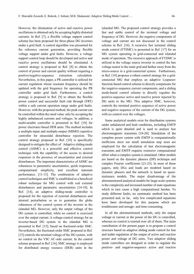
Assuming a transmission line connected between busbars

m and n in a typical MG as shown in Fig. (1-a), the

instantaneous voltage equation of this line in the

𝑎𝑏𝑐 reference frame is given by:

𝑣𝑎𝑏𝑐,𝑚(𝑡) − 𝑣𝑎𝑏𝑐,𝑛(𝑡) = 𝑣𝑎𝑏𝑐,𝑙(𝑡)

= 𝑅𝑖𝑎𝑏𝑐(𝑡) + 𝐿𝑑𝑖𝑎𝑏𝑐(𝑡)

𝑑𝑡

(1)

(a)

(b)

Fig.1. a) Representation of a typical transmission line, b) multi-

bus multi-DG MG

Transferring Eq. 1 to the 𝑑𝑞 synchronous reference frame

leads to:

𝑉𝑑𝑞𝑙𝑒 (𝑡) = 𝑅𝑉𝑑𝑞

𝑒 (𝑡) + 𝐿𝑑𝑉𝑑𝑞𝑙

𝑒

𝑑𝑡∓ 𝜔𝑠𝐿𝑉𝑞𝑑

𝑒 (𝑡) (2)

where, 𝜔𝑠 is the synchronous angular speed and

𝑉𝑑𝑞𝑙𝑒 (𝑡)and 𝑉𝑑𝑞

𝑒 (𝑡) are the fast time-variant space phasors

which define the time-varying phasors as:

�̅�𝑙(𝑡) = 𝑉𝑑𝑙𝑒 (𝑡) + 𝑗𝑉𝑞𝑙

𝑒 (𝑡), 𝐼�̅�(𝑡) = 𝐼𝑑𝑙𝑒 (𝑡) + 𝑗𝐼𝑞𝑙

𝑒 (𝑡) (3)

Considering (2), (3) it can be obtained that

�̅�𝑙(𝑡) = 𝑅𝐼�̅�(𝑡)+ 𝑗𝜔𝑠𝐿𝐼�̅�(𝑡) + 𝐿𝑑𝐼�̅�(𝑡)

𝑑𝑡

(4)

where; �̅�𝑙(𝑡) and 𝐼�̅�(𝑡) are the fast time-variant voltage

and current space phasors which describe high-frequency

effects. By ignoring the time derivative terms in Eq. 4

(which is the transient DC currents of the transmission

line), the slowly or quasi-state time-variant space phasors

are obtained as:

𝑉𝑙(𝑡) = 𝑅𝐼𝑙(𝑡)+ 𝑗𝜔𝑠𝐿𝐼𝑙(𝑡) (5)

where, 𝑉𝑙(𝑡) and 𝐼𝑙(𝑡) are the slowly time-variant voltage

and current space phasors. In fact, the quasi-state time-

variant assumption amounts to neglecting 𝑑𝐼�̅�(𝑡)

𝑑𝑡 term in

Eq. (4). By combining models of elementary passive

components, any symmetric transmission network can be

modeled based on the dq reference frame. The traditional

quasi-static model is based on the assumption that the

frequency of voltage and current signals throughout the

network is approximately constant. As a result, AC

signals can be modeled accurately enough by means of

time-varying phasors, and the transmission network can

be described by the constant admittance matrix Y through

the following linear relation [24]:

𝐼(𝑡) = 𝑌𝑉(𝑡) (6)

where 𝑌 is the admittance matrix of the n-bus network.

This is a quasi-static model of the transmission network,

since it is based on the assumption that phasors change

slowly in comparison to 𝜔𝑠. Based on this assumption,

the frequency is approximately constant throughout the

network and, as a result, matrix 𝑌𝑏𝑢𝑠 is composed of

constant admittances which are computed at fixed

frequency 𝜔𝑠 [24]. Extensive demonstration of Eq. 6 in

terms of d-q components of the voltage of the grid nodes

and the pure injectable currents can be expressed as Eq.

7. where 𝑔𝑖𝑗 and 𝑏𝑖𝑗 represent the real and imaginary part

of 𝑦𝑖𝑗 from Y bus admittance matrix of the network.

Direct comparison of these equations reveals that both

models are similar, except for the additional time

derivative terms in the dq0 model which describe high-

frequency effects. Note that, at low frequencies, where

the time derivatives are negligible, the two models are

equivalent in Ref. [25].

F. Shavakhi Zavareh, E. Rokrok, J. Soltani, M.R. Shakarami: Adaptive Sliding Mode Control … 68

[ 𝐼1𝑑

𝐼1𝑞

.

.

.𝐼𝑛𝑑

𝐼𝑛𝑞]

=

[ [

𝑔11 −𝑏11

𝑏11 𝑔11] [

𝑔12 −𝑏12

𝑏12 𝑔12] . . . [

𝑔1𝑛 −𝑏1𝑛

𝑏1𝑛 𝑔1𝑛]

.. . . . . . .. . . . . . .. . . . . . .

[𝑔𝑛1 −𝑏𝑛1

𝑏𝑛1 𝑔𝑛1] [

𝑔𝑛2 −𝑏𝑛2

𝑏𝑛2 𝑔𝑛2] . . . [

𝑔𝑛𝑛 −𝑏𝑛𝑛

𝑏𝑛𝑛 𝑔𝑛𝑛]]

[ 𝑉1𝑑

𝑉1𝑞

.

.

.𝑉𝑛𝑑

𝑉𝑛𝑞 ]

(7)

3. DYNAMIC FAULTS ANALYSIS OF THE

MICROGRID

3.1. Shunt Faults

It is well-known that, under unsymmetrical fault

conditions system voltages and currents can be written in

terms of different sequence (positive, negative, and zero)

components [20]. Under unsymmetrical faults, the DG

currents and voltages can be decomposed into

components due to positive-, negative-, and zero-

sequence components:

𝐼(𝑡) = 𝑌𝑉(𝑡),

𝐼 = 𝐼+ + 𝐼− + 𝐼0 , 𝑉 = 𝑉+ + 𝑉− + 𝑉0 (8)

Then, the connection between the DGs and MG can be

demonstrated by injecting the DG currents’ positive-,

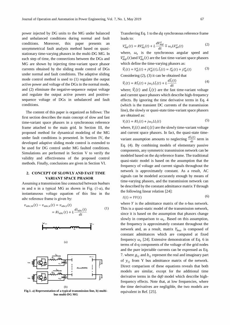
negative-, and zero-sequence components. Considering

an arbitrary shunt or series fault occurring at a certain

point (P) located in the MG network (Fig. (2)), the

conventional approach described in the power system

textbooks for shunt and series faults in the sinusoidal

steady-state conditions can be extended for the dynamic

analysis of these faults based on slowly fast time-variant

space phasors of networks as described here.

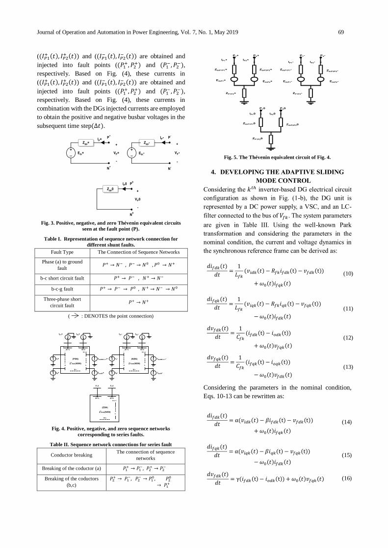
The Thévenin equivalent circuits corresponding to the

networks depicted in Fig. (2) can be obtained as shown

in Fig. (3). Using Fig. (3), the configuration of shunt

faults can be obtained as described in Table I [26]. Let us

consider a fictitious bus at the fault location in each

sequence network. In Fig. (3), 𝑍𝑃𝑃+ , 𝑍𝑃𝑃

− and 𝑍𝑃𝑃0 are the

deriving positive-, negative-, and zero-sequence

impedances corresponding to virtual bus (P) where the

fault occurs. Furthermore, 𝐸𝑡ℎ+ and 𝐸𝑡ℎ

− are the Thévenin

open-circuit voltages given by

𝐸𝑡ℎ+ = ∑ 𝑍𝑖𝑃

𝑀𝑖=1 𝐼𝑖

+(𝑡) + ∑ 𝑍𝑗𝑃𝐼𝑙𝑗+𝐿

𝑗=1 (𝑡),

𝐸𝑡ℎ− = ∑ 𝑍𝑖𝑃𝐼𝑖

−(𝑡)𝑀𝑖=1 + ∑ 𝑍𝑗𝑃𝐼𝑙𝑗

−(𝑡)𝐿𝑗=1

(9)

where; 𝐼𝑖 is the space current phasor injected by the 𝑖𝑡ℎ

DG to bus-bar (i) and 𝐼𝑙𝑗 is the space current phasor

injected by the 𝑗𝑡ℎ load. For each arbitrary shunt fault,

the Thévenin equivalent circuits are combined on the

basis of the information given in Table 1.

For an arbitrary shunt fault occurring in the MG, the

connections between MG networks’ sequences are

shown in Table I based on the application of slowly time-

variant space phasors. For a given shunt fault, by using

Thévenin equivalent circuits (Fig. (3)) and the

information given in Table I, the positive and negative

sequences’ fault currents defined by (𝐼𝑝+) and (𝐼𝑝

−) are

obtained and injected at fault points (𝑃+) and (𝑃−),

respectively (Fig. (2)). These currents in combination

with the DGs’ injected currents are used to obtain the

positive and negative busbar voltages corresponding to

these DGs in the subsequent time step (∆𝑡).

3.2. Series Faults

Series faults can occur along the power lines as the result

of an unbalanced series impedance condition of the lines

in the case of one or two broken lines. In practice, a series

fault is encountered, for example, when lines (or circuits)

are controlled by circuit breakers (or fuses) or any device

that does not open all three phases; one or two phases of

the line (or the circuit) may be open, while the other

phase(s) is closed. The present paper focuses on single-

and two-conductor breaking faults. Similar to the shunt

faults, the Thévenin equivalent circuits of Fig. (4) are

given in Fig. (5). Using these equivalent circuits and the

data in Table 2, these two types of series faults can be

studied with the same procedure described for the shunt

faults in the previous section.

Fig. 2. Positive, negative, and zero sequence networks

corresponding to shunt faults.

Referring to [26], the connections between power

sequences’ networks corresponding to a given series fault

are given Table 2.

Referring to Ref. [26], the equivalent Thévenin circuits

corresponding to Fig. (4) can be represented by the

following circuits. Assuming a type of series faults (one-

open-conductor or two-open-conductor) as shown in

Table 2, and using the Thévenin equivalent circuits

shown in Fig. (5), the positive and negative fault points

Journal of Operation and Automation in Power Engineering, Vol. 7, No. 1, May 2019 69

((𝐼𝑃1+ (𝑡), 𝐼𝑃2

+ (𝑡)) and ((𝐼𝑃1− (𝑡), 𝐼𝑃2

− (𝑡)) are obtained and

injected into fault points ((𝑃1+, 𝑃2

+) and (𝑃1− , 𝑃2

−),

respectively. Based on Fig. (4), these currents in

((𝐼𝑃1+ (𝑡), 𝐼𝑃2

+ (𝑡)) and ((𝐼𝑃1− (𝑡), 𝐼𝑃2

− (𝑡)) are obtained and

injected into fault points ((𝑃1+, 𝑃2

+) and (𝑃1− , 𝑃2

−),

respectively. Based on Fig. (4), these currents in

combination with the DGs injected currents are employed

to obtain the positive and negative busbar voltages in the

subsequent time step(∆𝑡).

Fig. 3. Positive, negative, and zero Thévenin equivalent circuits

seen at the fault point (P).

Table I. Representation of sequence network connection for

different shunt faults.

Fault Type The Connection of Sequence Networks

Phase (a) to ground

fault 𝑃+ → 𝑁− , 𝑃− → 𝑁0 , 𝑃0 → 𝑁+

b-c short circuit fault 𝑃+ → 𝑃− , 𝑁+ → 𝑁−

b-c-g fault 𝑃+ → 𝑃− → 𝑃0 , 𝑁+ → 𝑁− → 𝑁0

Three-phase short

circuit fault 𝑃+ → 𝑁+

( : DENOTES the point connection)

Fig. 4. Positive, negative, and zero sequence networks

corresponding to series faults.

Table II. Sequence network connections for series fault

Conductor breaking The connection of sequence

networks

Breaking of the coductor (a) 𝑃1+ → 𝑃1

− , 𝑃2+ → 𝑃2

−

Breaking of the coductors

(b,c)

𝑃2+ → 𝑃1

−, 𝑃2− → 𝑃1

0, 𝑃20

→ 𝑃1+

Fig. 5. The Thévenin equivalent circuit of Fig. 4.

4. DEVELOPING THE ADAPTIVE SLIDING

MODE CONTROL

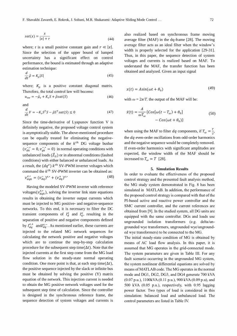
Considering the 𝑘𝑡ℎ inverter-based DG electrical circuit

configuration as shown in Fig. (1-b), the DG unit is

represented by a DC power supply, a VSC, and an LC-

filter connected to the bus of 𝑉𝑓𝑘 . The system parameters

are given in Table III. Using the well-known Park

transformation and considering the parameters in the

nominal condition, the current and voltage dynamics in

the synchronous reference frame can be derived as:

𝑑𝑖𝑓𝑑𝑘(𝑡)

𝑑𝑡=

1

𝐿𝑓𝑘(𝑣𝑖𝑑𝑘(𝑡) − 𝑅𝑓𝑘𝑖𝑓𝑑𝑘(t) − 𝑣𝑓𝑑𝑘(t))

+ 𝜔0(𝑡)𝑖𝑓𝑞𝑘(𝑡)

(10)

𝑑𝑖𝑓𝑞𝑘(𝑡)

𝑑𝑡=

1

𝐿𝑓𝑘(𝑣𝑖𝑞𝑘(𝑡) − 𝑅𝑓𝑘𝑖𝑞𝑘(t) − 𝑣𝑓𝑞𝑘(t))

− 𝜔0(𝑡)𝑖𝑓𝑑𝑘(𝑡)

(11)

𝑑𝑣𝑓𝑑𝑘(𝑡)

𝑑𝑡=

1

𝐶𝑓𝑘(𝑖𝑓𝑑𝑘(t) − 𝑖𝑜𝑑𝑘(t))

+ 𝜔0(𝑡)𝑣𝑓𝑞𝑘(𝑡)

(12)

𝑑𝑣𝑓𝑞𝑘(𝑡)

𝑑𝑡=

1

𝐶𝑓𝑘(𝑖𝑓𝑞𝑘(t) − 𝑖𝑜𝑞𝑘(t))

− 𝜔0(𝑡)𝑣𝑓𝑑𝑘(𝑡)

(13)

Considering the parameters in the nominal condition,

Eqs. 10-13 can be rewritten as:

𝑑𝑖𝑓𝑑𝑘(𝑡)

𝑑𝑡= α(𝑣𝑖𝑑𝑘(𝑡) − 𝛽𝑖𝑓𝑑𝑘(t) − 𝑣𝑓𝑑𝑘(t))

+ 𝜔0(𝑡)𝑖𝑓𝑞𝑘(𝑡)

(14)

𝑑𝑖𝑓𝑞𝑘(𝑡)

𝑑𝑡= α(𝑣𝑖𝑞𝑘(𝑡) − 𝛽𝑖𝑞𝑘(t) − 𝑣𝑓𝑞𝑘(t))

− 𝜔0(𝑡)𝑖𝑓𝑑𝑘(𝑡) (15)

𝑑𝑣𝑓𝑑𝑘(𝑡)

𝑑𝑡= γ(𝑖𝑓𝑑𝑘(t) − 𝑖𝑜𝑑𝑘(t)) + 𝜔0(𝑡)𝑣𝑓𝑞𝑘(𝑡) (16)

F. Shavakhi Zavareh, E. Rokrok, J. Soltani, M.R. Shakarami: Adaptive Sliding Mode Control … 70

𝑑𝑣𝑓𝑞𝑘(𝑡)

𝑑𝑡= γ(𝑖𝑓𝑞𝑘(t) − 𝑖𝑜𝑞𝑘(t)) − 𝜔0(𝑡)𝑣𝑓𝑑𝑘(𝑡) (17)

where 𝛼 =1

𝐿𝑓𝑘, 𝛽 = 𝑅𝑓𝑘 , 𝛾 =

1

𝐶𝑓𝑘 are the nominal

parameter values. If the parameters of the system deviate

from their nominal values, Eqs. 14-17 can be modified

as:

𝑑𝑖𝑓𝑑𝑘(𝑡)

𝑑𝑡= α(𝑣𝑖𝑑𝑘(𝑡) − 𝛽𝑖𝑓𝑑𝑘(t) − 𝑣𝑓𝑑𝑘(t))

+ 𝜔0(𝑡)𝑖𝑓𝑞𝑘(𝑡) + 𝜂𝑑

(18)

𝑑𝑖𝑓𝑞𝑘(𝑡)

𝑑𝑡= α(𝑣𝑖𝑞𝑘(𝑡) − 𝛽𝑖𝑞𝑘(t) − 𝑣𝑓𝑞𝑘(t))

− 𝜔0(𝑡)𝑖𝑓𝑑𝑘(𝑡) + 𝜂𝑞

(19)

𝑑𝑣𝑓𝑑𝑘(𝑡)

𝑑𝑡= γ(𝑖𝑓𝑑𝑘(t) − 𝑖𝑜𝑑𝑘(t)) + 𝜔0(𝑡)𝑣𝑓𝑞𝑘(𝑡)

+ 𝜗𝑑

(20)

𝑑𝑣𝑓𝑞𝑘(𝑡)

𝑑𝑡= γ(𝑖𝑓𝑞𝑘(t) − 𝑖𝑜𝑞𝑘(t)) − 𝜔0(𝑡)𝑣𝑓𝑑𝑘(𝑡)

+ 𝜗𝑞

(21)

where 𝜂𝑑𝑞 and 𝜗𝑑𝑞 are the lumped-sum uncertainties

which can be written as:

𝜂𝑑𝑞 = Δα(𝑣𝑖𝑑𝑞𝑘(𝑡) − 𝛽𝑖𝑓𝑑𝑞𝑘(𝑡) − 𝑣𝑓𝑑𝑞𝑘(𝑡)) −

Δ𝛽(𝛼 + Δ𝛼)𝑖𝑓𝑑𝑞𝑘(𝑡) + 𝛿𝑑𝑞

𝜗𝑑𝑞 = Δγ(𝑖𝑓𝑑𝑞𝑘(t) − 𝑖𝑜𝑑𝑞𝑘(t)) + 𝜈𝑑𝑞

(22)

where Δ denotes a difference from the nominal value and

the terms 𝛿𝑑𝑞 and 𝜈𝑑𝑞 are added to account for system

dynamic disturbances and other un-modeled

uncertainties.

It is assumed that the LC-filter and interlink-line have

balanced three-phase impedance since each equation (10)

to (13) can be fully decoupled into positive and negative

sequences. Under the unbalanced condition, each voltage

and current can be expressed as:

𝑣𝑓𝑑 = 𝑣𝑓𝑑+ + 𝑣𝑓𝑑

− , 𝑣𝑓𝑞 = 𝑣𝑓𝑞+ + 𝑣𝑓𝑞

−

𝑖𝑓𝑑 = 𝑖𝑓𝑑+ + 𝑖𝑓𝑑

− , 𝑖𝑓𝑞 = 𝑖𝑓𝑞+ + 𝑖𝑓𝑞

− (23)

It must be noted that in the dq coordinate [20]:

1) Positive-sequence DG quantities appear as DC

values; and

2) Negative-sequence DG quantities exhibit the

second harmonics of fundamental frequency and are,

therefore, time-variant.

Instantaneous active and reactive power injected by

the DG unit to the MG can be represented as:

𝑃𝑓 =3

2(𝑣𝑓𝑑(𝑡)𝑖𝑓𝑑(𝑡) + 𝑣𝑓𝑞(𝑡)𝑖𝑓𝑞(𝑡))

𝑄𝑓 =3

2(𝑣𝑓𝑞(𝑡)𝑖𝑓𝑑(𝑡) − 𝑣𝑓𝑑(𝑡)𝑖𝑓𝑞(𝑡))

(24)

The proposed control structure consists of an adaptive

sliding mode based on the positive and negative power

controller on the reference values of ( 𝑃𝑓+,∗ , 𝑣𝑓

+,∗ ) and

(𝑃𝑓−,∗ = 0, 𝑣𝑓

−,∗ = 0). The positive power controller is

designed to regulate the positive sequence of active and

reactive power injected by the DG unit to the MG,

whereas the negative power controller is designed to

compensate for the impact of negative sequence voltage

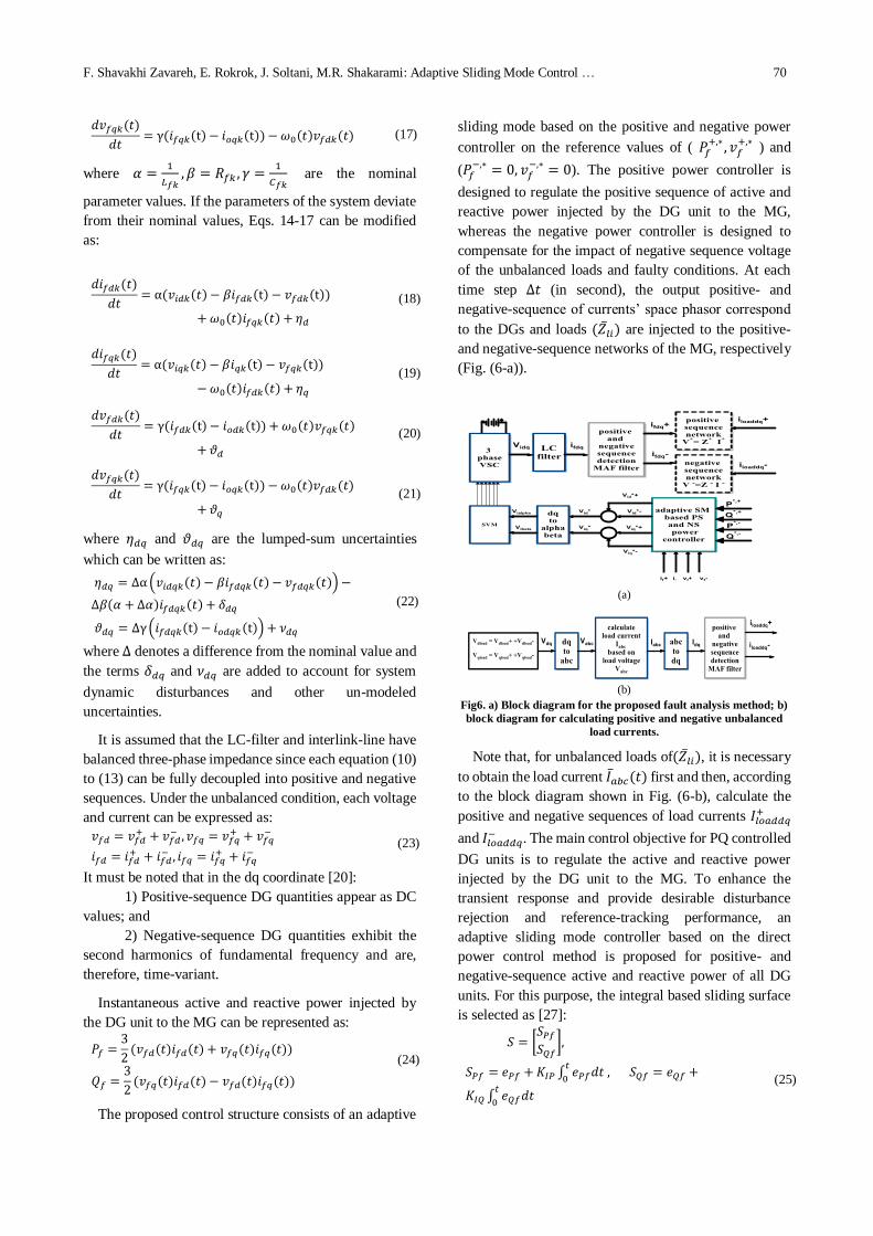
of the unbalanced loads and faulty conditions. At each

time step ∆𝑡 (in second), the output positive- and

negative-sequence of currents’ space phasor correspond

to the DGs and loads (�̅�𝑙𝑖) are injected to the positive-

and negative-sequence networks of the MG, respectively

(Fig. (6-a)).

(a)

(b)

Fig6. a) Block diagram for the proposed fault analysis method; b)

block diagram for calculating positive and negative unbalanced

load currents.

Note that, for unbalanced loads of(�̅�𝑙𝑖), it is necessary

to obtain the load current 𝐼�̅�𝑏𝑐(𝑡) first and then, according

to the block diagram shown in Fig. (6-b), calculate the

positive and negative sequences of load currents 𝐼𝑙𝑜𝑎𝑑𝑑𝑞+

and 𝐼𝑙𝑜𝑎𝑑𝑑𝑞− . The main control objective for PQ controlled

DG units is to regulate the active and reactive power

injected by the DG unit to the MG. To enhance the

transient response and provide desirable disturbance

rejection and reference-tracking performance, an

adaptive sliding mode controller based on the direct

power control method is proposed for positive- and

negative-sequence active and reactive power of all DG

units. For this purpose, the integral based sliding surface

is selected as [27]:

𝑆 = [𝑆𝑃𝑓

𝑆𝑄𝑓],

𝑆𝑃𝑓 = 𝑒𝑃𝑓 + 𝐾𝐼𝑃 ∫ 𝑒𝑃𝑓𝑑𝑡𝑡

0 , 𝑆𝑄𝑓 = 𝑒𝑄𝑓 +

𝐾𝐼𝑄 ∫ 𝑒𝑄𝑓𝑑𝑡𝑡

0

(25)

Journal of Operation and Automation in Power Engineering, Vol. 7, No. 1, May 2019 71

where 𝐾𝐼𝑃 and 𝐾𝐼𝑄 are positive constant gains and𝑒𝑃𝑓,

𝑒𝑄𝑓 are the error signals corresponding to the output

active and reactive powers and voltage of the DG, given

by:

𝑒𝑃𝑓 = 𝑃𝑓∗ − 𝑃𝑓, 𝑒𝑄𝑓 = 𝑄𝑓

∗ − 𝑄𝑓 (26)

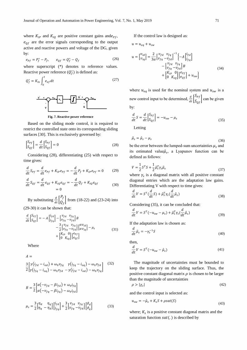
where superscript (*) denotes to reference values.

Reactive power reference (𝑄𝑓∗) is defined as:

𝑄𝑓∗ = 𝐾𝐼𝑣 ∫ 𝑒𝑣𝑓𝑑𝑡

𝑡

0

(27)

Fig. 7. Reactive power reference

Based on the sliding mode control, it is required to

restrict the controlled state onto its corresponding sliding

surfaces [30]. This is exclusively governed by:

[𝑆𝑃𝑓

𝑆𝑄𝑓] =

𝑑

𝑑𝑡[𝑆𝑃𝑓

𝑆𝑄𝑓] = 0 (28)

Considering (28), differentiating (25) with respect to

time gives:

𝑑

𝑑𝑡𝑆𝑃𝑓 =

𝑑

𝑑𝑡𝑒𝑃𝑓 + 𝐾𝐼𝑃𝑒𝑃𝑓 = −

𝑑

𝑑𝑡𝑃𝑓 + 𝐾𝐼𝑃𝑒𝑃𝑓 = 0 (29)

𝑑

𝑑𝑡𝑆𝑄𝑓 =

𝑑

𝑑𝑡𝑒𝑄𝑓 + 𝐾𝐼𝑄𝑒𝑄𝑓 = −

𝑑

𝑑𝑡𝑄𝑓 + 𝐾𝐼𝑄𝑒𝑄𝑓

= 0

(30)

By substituting 𝑑

𝑑𝑡[𝑃𝑓

𝑄𝑓] from (18-22) and (23-24) into

(29-30) it can be shown that:

𝑑

𝑑𝑡[𝑆𝑃𝑓

𝑆𝑄𝑓] = − 𝐴 [

𝑖𝑓𝑑

𝑖𝑓𝑞] − [

𝑣𝑓𝑑 𝑣𝑓𝑞

𝑣𝑓𝑞 −𝑣𝑓𝑑] 𝐵

−3

2[𝑣𝑓𝑑 𝑣𝑓𝑞

𝑣𝑓𝑞 −𝑣𝑓𝑑] [

𝛼𝑣𝑖𝑑

𝛼𝑣𝑖𝑞] − 𝜇𝑠

+ [𝐾𝐼𝑃 00 𝐾𝐼𝑄

] [𝑒𝑃𝑓

𝑒𝑄𝑓]

(31)

Where

If the control law is designed as:

𝑢 = 𝑢𝑒𝑞 + 𝑢𝑠𝑤

𝑢 = [𝑣𝑖𝑑

𝑣𝑖𝑞] =

2

3𝛼[𝑣𝑓𝑑 𝑣𝑓𝑞

𝑣𝑓𝑞 −𝑣𝑓𝑑]−1

{−𝐴 [𝑖𝑓𝑑

𝑖𝑓𝑞]

− [𝑣𝑓𝑑 𝑣𝑓𝑞

𝑣𝑓𝑞 −𝑣𝑓𝑑]𝐵

+ [𝐾𝐼𝑃 00 𝐾𝐼𝑄

] [𝑒𝑃𝑓

𝑒𝑄𝑓] + 𝑢𝑠𝑤}

(34)

where 𝑢𝑒𝑞 is used for the nominal system and 𝑢𝑠𝑤 is a

new control input to be determined, 𝑑

𝑑𝑡[𝑆𝑃𝑓

𝑆𝑄𝑓] can be given

by:

𝑑

𝑑𝑡𝑆 =

𝑑

𝑑𝑡[𝑆𝑃𝑓

𝑆𝑄𝑓] = −𝑢𝑠𝑤 − 𝜇𝑠

(35)

Letting

𝜇𝑠 = �̂�𝑠 − 𝜇𝑠

(36)

be the error between the lumped-sum uncertainties 𝜇𝑠 and

its estimated value�̂�𝑠, a Lyapunov function can be

defined as follows:

𝑉 =1

2𝑆𝑇𝑆 +

1

2𝜇𝑠

𝑇𝛾𝑠𝜇𝑠

(37)

where 𝛾𝑠 is a diagonal matrix with all positive constant

diagonal entries which are the adaptation law gains.

Differentiating V with respect to time gives:

𝑑

𝑑𝑡𝑉 = 𝑆𝑇(

𝑑

𝑑𝑡𝑆) + 𝜇𝑠

𝑇𝛾𝑠(𝑑

𝑑𝑡𝜇𝑠)

(38)

Considering (35), it can be concluded that:

𝑑

𝑑𝑡𝑉 = 𝑆𝑇(−𝑢𝑠𝑤 − 𝜇𝑠) + 𝜇𝑠

𝑇𝛾𝑠(𝑑

𝑑𝑡𝜇𝑠)

(39)

If the adaptation law is chosen as:

𝑑

𝑑𝑡𝜇𝑠 = −𝛾𝑠

−1𝑆

(40)

then, 𝑑

𝑑𝑡𝑉 = 𝑆𝑇(−𝑢𝑠𝑤 − �̂�𝑠) (41)

The magnitude of uncertainties must be bounded to

keep the trajectory on the sliding surface. Thus, the

positive constant diagonal matrix 𝜌 is chosen to be larger

than the magnitude of uncertainties

𝜌 > |𝜒𝑠| (42)

and the control input is selected as:

𝑢𝑠𝑤 = −�̂�𝑠 + 𝐾𝑠𝑆 + 𝜌𝑠𝑎𝑡(𝑆)

(43)

where; 𝐾𝑠 is a positive constant diagonal matrix and the

saturation function 𝑠𝑎𝑡(. ) is described by

𝐴 =

3

2[𝛾(𝑖𝑓𝑑 − 𝑖𝑜𝑑) + 𝜔0𝑣𝑓𝑞 𝛾(𝑖𝑓𝑞 − 𝑖𝑜𝑞) − 𝜔0𝑣𝑓𝑑

𝛾(𝑖𝑓𝑞 − 𝑖𝑜𝑞) − 𝜔0𝑣𝑓𝑑 − 𝛾(𝑖𝑓𝑑 − 𝑖𝑜𝑑) − 𝜔0𝑣𝑓𝑞

] (32)

𝐵 =3

2[𝛼(−𝑣𝑓𝑑 − 𝛽𝑖𝑓𝑑) + 𝜔0𝑖𝑓𝑞

𝛼(−𝑣𝑓𝑞 − 𝛽𝑖𝑓𝑞) − 𝜔0𝑖𝑓𝑑

]

𝜇𝑠 =3

2[𝜂𝑑 𝜂𝑞

𝜂𝑞 − 𝜂𝑑] [

𝑖𝑓𝑑

𝑖𝑓𝑞] +

3

2[𝑣𝑓𝑑 𝑣𝑓𝑞

𝑣𝑓𝑞 −𝑣𝑓𝑑] [

𝜗𝑑

𝜗𝑞] (33)

F. Shavakhi Zavareh, E. Rokrok, J. Soltani, M.R. Shakarami: Adaptive Sliding Mode Control … 72

𝑠𝑎𝑡(𝑥) =𝑥

|𝑥| + 𝑟

(44)

where; r is a small positive constant gain and 𝑟 ≪ |𝑥|.

Since the selection of the upper bound of lumped

uncertainty has a significant effect on control

performance, the bound is estimated through an adaptive

estimation technique: 𝑑

𝑑𝑡�̂� = 𝐾𝜌|𝑆| (45)

where; 𝐾𝜌 is a positive constant diagonal matrix.

Therefore, the total control law will become:

𝑢𝑠𝑤 = −�̂�𝑠 + 𝐾𝑠𝑆 + �̂�𝑠𝑎𝑡(𝑆) (46)

and 𝑑

𝑑𝑡𝑉 = −𝐾𝑠𝑆

𝑇𝑆 − �̂�𝑆𝑇𝑠𝑎𝑡(𝑆) ≤ 0 (47)

Since the time-derivative of Lyapunov function V is

definitely negative, the proposed voltage control system

is asymptotically stable. The above-mentioned procedure

can be equally treated for eliminating the negative-

sequence components of the 𝑘𝑡ℎ DG voltage busbar

(𝑣𝑑𝑘−,∗ = 0, 𝑣𝑞𝑘

−,∗ = 0) in normal operating conditions with

unbalanced loads (�̅�𝑙𝑖) or in abnormal conditions (faulted

conditions) with either balanced or unbalanced loads. As

a result, the (𝑑𝑞𝑒) 𝑘𝑡ℎ SV-PWM inverter voltages which

command the 𝑘𝑡ℎ SV-PWM inverter can be obtained as:

𝑣𝑑𝑞𝑘𝑒,∗ = (𝑣𝑑𝑞

− )𝑒,∗ + (𝑣𝑑𝑞+ )𝑒,∗ (48)

Having the modeled SV-PWM inverter with reference

voltages(𝑣𝑑𝑞𝑘𝑒,∗ ), solving the inverter link state equations

results in obtaining the inverter output currents which

must be injected to MG positive- and negative-sequence

networks. To this end, it is necessary to filter the DC

transient components of 𝐼𝑑𝑒 and 𝐼𝑞

𝑒 , resulting in the

separation of positive and negative components defined

by 𝐼𝑑𝑞𝑒,+

and𝐼𝑑𝑞𝑒.−. As mentioned earlier, these currents are

injected to the related MG network sequences for

calculating the network positive and negative voltages

which are to continue the step-by-step calculation

procedure for the subsequent step time(∆𝑡). Note that the

injected currents at the first step come from the MG load

flow solution in the steady-state normal operating

condition. One more point is that, at each step time(∆𝑡),

the positive sequence injected by the slack or infinite bus

must be obtained by solving the positive (Y) matrix

equation of the network. This injection current is needed

to obtain the MG positive network voltages used for the

subsequent step time of calculation. Since the controller

is designed in the synchronous reference frame, the

sequence detection of system voltages and currents is

also realized based on synchronous frame moving

average filter (MAF) in the dq-frame [28]. The moving

average filter acts as an ideal filter when the window’s

width is properly selected for the application [29-31].

Thus, in this paper, the sequence detection of system

voltages and currents is realized based on MAF. To

understand the MAF, the transfer function has been

obtained and analyzed. Given an input signal

𝑥(𝑡) = 𝐴𝑠𝑖𝑛(𝜔𝑡 + 𝜃0) (49)

with ω = 2π/T, the output of the MAF will be:

�̅�(t) =𝐴

𝜔𝑇𝜔

{𝐶𝑜𝑠[𝜔(𝑡 − 𝑇𝜔) + 𝜃0]

− 𝐶𝑜𝑠(𝜔𝑡 + 𝜃0)}

(50)

when using the MAF to filter 𝑑𝑞 components, if 𝑇𝜔 =𝑇

2,

the 𝑑𝑞 even-order oscillations from odd-order harmonics

and the negative sequence would be completely removed.

If even-order harmonics with significant amplitudes are

expected, the window width of the MAF should be

increased to 𝑇𝜔 = 𝑇 [28].

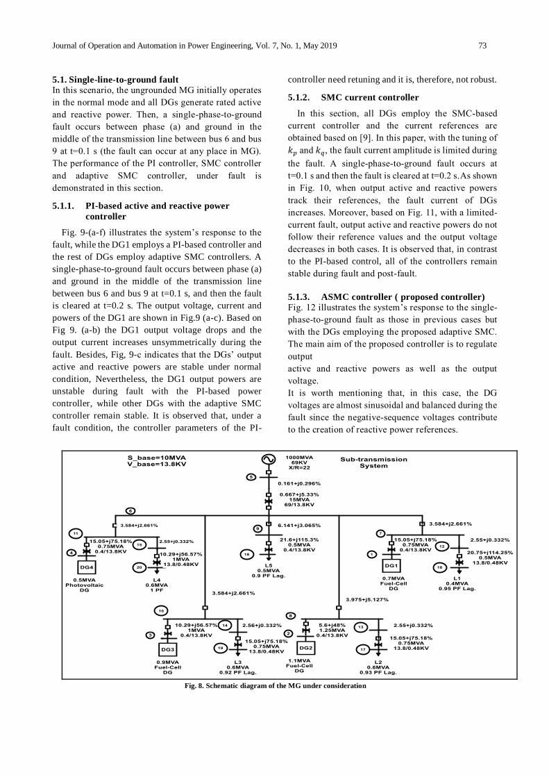
5. Simulation Results

In order to evaluate the effectiveness of the proposed

control strategy and the presented fault analysis method,

the MG study system demonstrated in Fig. 8 has been

simulated in MATLAB. In addition, the performance of

the proposed control strategy is compared with that of the

PI-based active and reactive power controller and the

SMC current controller, and the current references are

obtained from [9]. In the studied system, all DG units are

equipped with the same controller. DGs and loads use

ungrounded isolation transformers (e.g. delta/un-

grounded wye transformers, ungrounded wye/unground-

ed wye transformers) to be connected to the MG.

The initial steady-state condition of MG is obtained by

means of AC load flow analysis. In this paper, it is

assumed that MG operates in the grid-connected mode.

The system parameters are given in Table III. For any

fault scenario occurring in the ungrounded MG system,

the system nonlinear differential equations are solved by

means of MATLAB code. The MG operates in the normal

mode and DG1, DG2, DG3, and DG4 generate 700 kVA

(0.07 p.u.), 1100kVA (0.11 p.u.), 900 kVA (0.09 p.u), and

500 kVA (0.05 p.u.), respectively, with 0.95 lagging

power factor. Two types of load is considered in this

simulation: balanced load and unbalanced load. The

control parameters are listed in Table IV.

Journal of Operation and Automation in Power Engineering, Vol. 7, No. 1, May 2019 73

5.1. Single-line-to-ground fault

In this scenario, the ungrounded MG initially operates

in the normal mode and all DGs generate rated active

and reactive power. Then, a single-phase-to-ground

fault occurs between phase (a) and ground in the

middle of the transmission line between bus 6 and bus

9 at t=0.1 s (the fault can occur at any place in MG).

The performance of the PI controller, SMC controller

and adaptive SMC controller, under fault is

demonstrated in this section.

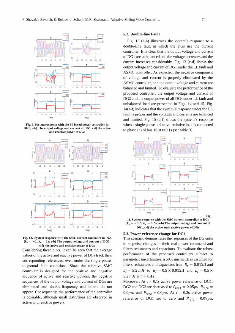
5.1.1. PI-based active and reactive power

controller

Fig. 9-(a-f) illustrates the system’s response to the

fault, while the DG1 employs a PI-based controller and

the rest of DGs employ adaptive SMC controllers. A

single-phase-to-ground fault occurs between phase (a)

and ground in the middle of the transmission line

between bus 6 and bus 9 at t=0.1 s, and then the fault

is cleared at t=0.2 s. The output voltage, current and

powers of the DG1 are shown in Fig.9 (a-c). Based on

Fig 9. (a-b) the DG1 output voltage drops and the

output current increases unsymmetrically during the

fault. Besides, Fig, 9-c indicates that the DGs’ output

active and reactive powers are stable under normal

condition, Nevertheless, the DG1 output powers are

unstable during fault with the PI-based power

controller, while other DGs with the adaptive SMC

controller remain stable. It is observed that, under a

fault condition, the controller parameters of the PI-

controller need retuning and it is, therefore, not robust.

5.1.2. SMC current controller

In this section, all DGs employ the SMC-based

current controller and the current references are

obtained based on [9]. In this paper, with the tuning of

𝑘𝑝 and 𝑘𝑞, the fault current amplitude is limited during

the fault. A single-phase-to-ground fault occurs at

t=0.1 s and then the fault is cleared at t=0.2 s.As shown

in Fig. 10, when output active and reactive powers

track their references, the fault current of DGs

increases. Moreover, based on Fig. 11, with a limited-

current fault, output active and reactive powers do not

follow their reference values and the output voltage

decreases in both cases. It is observed that, in contrast

to the PI-based control, all of the controllers remain

stable during fault and post-fault.

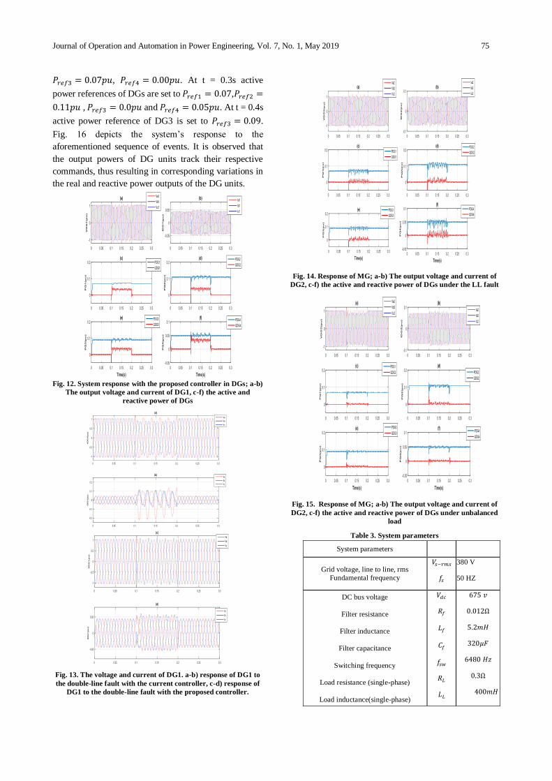
5.1.3. ASMC controller ( proposed controller)

Fig. 12 illustrates the system’s response to the single-

phase-to-ground fault as those in previous cases but

with the DGs employing the proposed adaptive SMC.

The main aim of the proposed controller is to regulate

output

active and reactive powers as well as the output

voltage.

It is worth mentioning that, in this case, the DG

voltages are almost sinusoidal and balanced during the

fault since the negative-sequence voltages contribute

to the creation of reactive power references.

Fig. 8. Schematic diagram of the MG under consideration

F. Shavakhi Zavareh, E. Rokrok, J. Soltani, M.R. Shakarami: Adaptive Sliding Mode Control … 74

Fig. 9. System response with the PI-based power controller in

DG1; a-b) The output voltage and current of DG1, c-f) the active

and reactive power of DGs

Fig. 10. System response with the SMC current controller in DGs

(𝒌𝒑 = −𝟏, 𝒌𝒒 = 𝟏); a-b) The output voltage and current of DG1,

c-f) the active and reactive power of DGs

Considering these plots, it can be seen that the average

values of the active and reactive power of DGs track their

corresponding references, even under the single-phase-

to-ground fault conditions. Since the adaptive SMC

controller is designed for the positive and negative

sequence of active and reactive powers, the negative

sequences of the output voltage and current of DGs are

eliminated and double-frequency oscillations do not

appear. Consequently, the performance of the controller

is desirable, although small distortions are observed in

active and reactive powers.

5.2. Double-line Fault

Fig. 13 (a-b) illustrates the system’s response to a

double-line fault in which the DGs use the current

controller. It is clear that the output voltage and current

of DG1 are unbalanced and the voltage decreases and the

current increases considerably. Fig. 13 (c-d) shows the

output voltage and current of DG1 under the LL fault and

ASMC controller. As expected, the negative component

of voltage and current is properly eliminated by the

ASMC controller, and the output voltage and current are

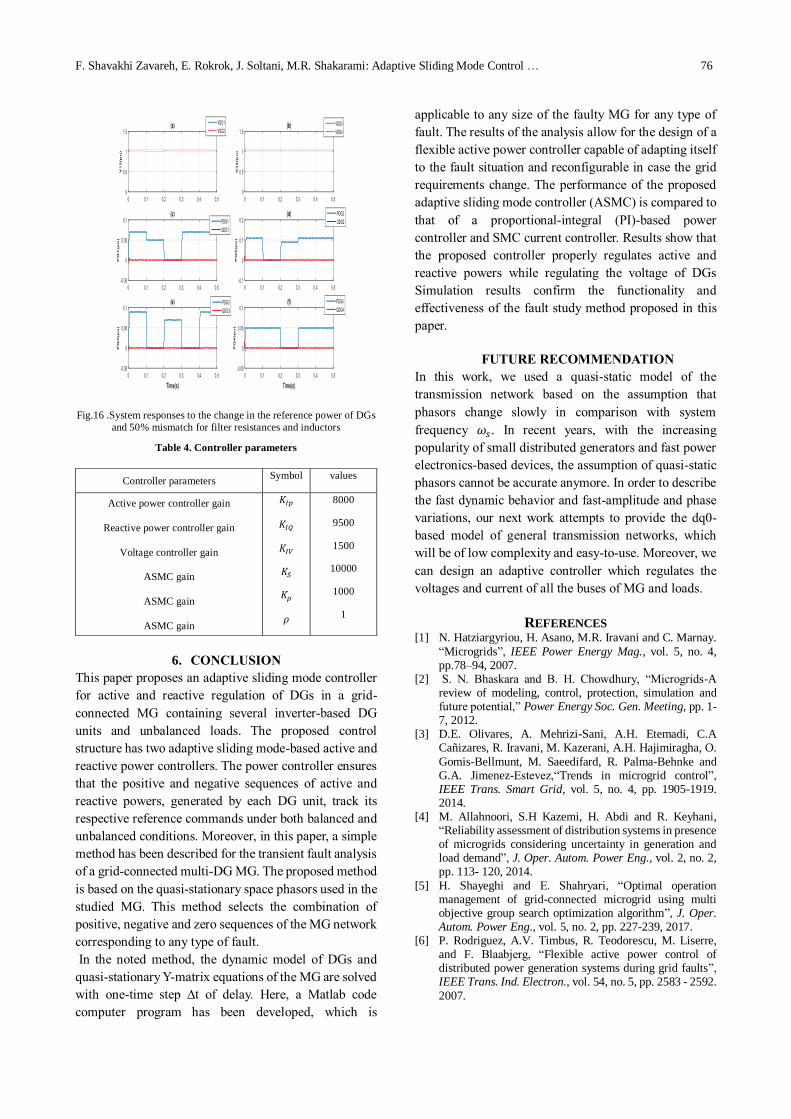
balanced and limited. To evaluate the performance of the

proposed controller, the output voltage and current of

DG2 and the output power of all DGs under LL fault and

unbalanced load are presented in Figs. 14 and 15. Fig.

14(a-f) indicates that the system’s response under the LL

fault is proper and the voltages and currents are balanced

and limited. Fig. 15 (a-f) shows the system’s response

when a single phase inductive-resistive load is connected

to phase (a) of bus 16 at t=0.1s (see table 3).

Fig.

11. System response with the SMC current controller in DGs

(𝒌𝒑 = −𝟎. 𝟓, 𝒌𝒒 = 𝟎. 𝟓); a-b) The output voltage and current of

DG1, c-f) the active and reactive power of DGs

5.3. Power reference change for DG1

This scenario demonstrates the responses of the DG units

to stepwise changes in their real power command and

filters resistances and capacitors. To evaluate the robust

performance of the proposed controllers subject to

parametric uncertainties, a 50% mismatch is assumed for

filters resistances and capacitors from 𝑅𝑓 = 0.012Ω and

𝐿𝑓 = 5.2 𝑚𝐻 to 𝑅𝑓 = 0.5 × 0.012Ω and 𝐿𝑓 = 0.5 ×

5.2 𝑚𝐻 at 𝑡 = 0.4𝑠.

Moreover. At t = 0.1s active power reference of DG1,

DG2 and DG3 are decreased to 𝑃𝑟𝑒𝑓1 = 0.05𝑝𝑢, 𝑃𝑟𝑒𝑓2 =

0.0𝑝𝑢, and 𝑃𝑟𝑒𝑓3 = 0.0𝑝𝑢. At t = 0.2s active power

reference of DG1 set to zero and 𝑃𝑟𝑒𝑓2 = 0.09𝑝𝑢,

Journal of Operation and Automation in Power Engineering, Vol. 7, No. 1, May 2019 75

𝑃𝑟𝑒𝑓3 = 0.07𝑝𝑢, 𝑃𝑟𝑒𝑓4 = 0.00𝑝𝑢. At t = 0.3s active

power references of DGs are set to 𝑃𝑟𝑒𝑓1 = 0.07,𝑃𝑟𝑒𝑓2 =

0.11𝑝𝑢 , 𝑃𝑟𝑒𝑓3 = 0.0𝑝𝑢 and 𝑃𝑟𝑒𝑓4 = 0.05𝑝𝑢. At t = 0.4s

active power reference of DG3 is set to 𝑃𝑟𝑒𝑓3 = 0.09.

Fig. 16 depicts the system’s response to the

aforementioned sequence of events. It is observed that

the output powers of DG units track their respective

commands, thus resulting in corresponding variations in

the real and reactive power outputs of the DG units.

Fig. 12. System response with the proposed controller in DGs; a-b)

The output voltage and current of DG1, c-f) the active and

reactive power of DGs

Fig. 13. The voltage and current of DG1. a-b) response of DG1 to

the double-line fault with the current controller, c-d) response of

DG1 to the double-line fault with the proposed controller.

Fig. 14. Response of MG; a-b) The output voltage and current of

DG2, c-f) the active and reactive power of DGs under the LL fault

Fig. 15. Response of MG; a-b) The output voltage and current of

DG2, c-f) the active and reactive power of DGs under unbalanced

load

Table 3. System parameters

System parameters

Grid voltage, line to line, rms

Fundamental frequency

𝑉𝑠−𝑟𝑚𝑠

𝑓𝑠

380 V

50 HZ

DC bus voltage

Filter resistance

Filter inductance

Filter capacitance

Switching frequency

Load resistance (single-phase)

Load inductance(single-phase)

𝑉𝑑𝑐

𝑅𝑓

𝐿𝑓

𝐶𝑓

𝑓𝑠𝑤

𝑅𝐿

𝐿𝐿

675 𝑣

0.012Ω

5.2𝑚𝐻

320𝜇𝐹

6480 𝐻𝑧

0.3Ω

400𝑚𝐻

F. Shavakhi Zavareh, E. Rokrok, J. Soltani, M.R. Shakarami: Adaptive Sliding Mode Control … 76

Fig.16 .System responses to the change in the reference power of DGs

and 50% mismatch for filter resistances and inductors

Table 4. Controller parameters

6. CONCLUSION

This paper proposes an adaptive sliding mode controller

for active and reactive regulation of DGs in a grid-

connected MG containing several inverter-based DG

units and unbalanced loads. The proposed control

structure has two adaptive sliding mode-based active and

reactive power controllers. The power controller ensures

that the positive and negative sequences of active and

reactive powers, generated by each DG unit, track its

respective reference commands under both balanced and

unbalanced conditions. Moreover, in this paper, a simple

method has been described for the transient fault analysis

of a grid-connected multi-DG MG. The proposed method

is based on the quasi-stationary space phasors used in the

studied MG. This method selects the combination of

positive, negative and zero sequences of the MG network

corresponding to any type of fault.

In the noted method, the dynamic model of DGs and

quasi-stationary Y-matrix equations of the MG are solved

with one-time step ∆t of delay. Here, a Matlab code

computer program has been developed, which is

applicable to any size of the faulty MG for any type of

fault. The results of the analysis allow for the design of a

flexible active power controller capable of adapting itself

to the fault situation and reconfigurable in case the grid

requirements change. The performance of the proposed

adaptive sliding mode controller (ASMC) is compared to

that of a proportional-integral (PI)-based power

controller and SMC current controller. Results show that

the proposed controller properly regulates active and

reactive powers while regulating the voltage of DGs

Simulation results confirm the functionality and

effectiveness of the fault study method proposed in this

paper.

FUTURE RECOMMENDATION

In this work, we used a quasi-static model of the

transmission network based on the assumption that

phasors change slowly in comparison with system

frequency 𝜔𝑠. In recent years, with the increasing

popularity of small distributed generators and fast power

electronics-based devices, the assumption of quasi-static

phasors cannot be accurate anymore. In order to describe

the fast dynamic behavior and fast-amplitude and phase

variations, our next work attempts to provide the dq0-

based model of general transmission networks, which

will be of low complexity and easy-to-use. Moreover, we

can design an adaptive controller which regulates the

voltages and current of all the buses of MG and loads.

REFERENCES [1] N. Hatziargyriou, H. Asano, M.R. Iravani and C. Marnay.

“Microgrids”, IEEE Power Energy Mag., vol. 5, no. 4, pp.78–94, 2007.

[2] S. N. Bhaskara and B. H. Chowdhury, “Microgrids-A review of modeling, control, protection, simulation and future potential,” Power Energy Soc. Gen. Meeting, pp. 1-7, 2012.

[3] D.E. Olivares, A. Mehrizi-Sani, A.H. Etemadi, C.A Cañizares, R. Iravani, M. Kazerani, A.H. Hajimiragha, O.

Gomis-Bellmunt, M. Saeedifard, R. Palma-Behnke and G.A. Jimenez-Estevez,“Trends in microgrid control”, IEEE Trans. Smart Grid, vol. 5, no. 4, pp. 1905-1919. 2014.

[4] M. Allahnoori, S.H Kazemi, H. Abdi and R. Keyhani, “Reliability assessment of distribution systems in presence of microgrids considering uncertainty in generation and load demand”, J. Oper. Autom. Power Eng., vol. 2, no. 2, pp. 113- 120, 2014.

[5] H. Shayeghi and E. Shahryari, “Optimal operation management of grid-connected microgrid using multi objective group search optimization algorithm”, J. Oper. Autom. Power Eng., vol. 5, no. 2, pp. 227-239, 2017.

[6] P. Rodriguez, A.V. Timbus, R. Teodorescu, M. Liserre, and F. Blaabjerg, “Flexible active power control of distributed power generation systems during grid faults”, IEEE Trans. Ind. Electron., vol. 54, no. 5, pp. 2583 - 2592.

2007.

Controller parameters Symbol values

Active power controller gain

Reactive power controller gain

Voltage controller gain

ASMC gain

ASMC gain

ASMC gain

𝐾𝐼𝑝

𝐾𝐼𝑄

𝐾𝐼𝑉

𝐾𝑆

𝐾𝜌

𝜌

8000

9500

1500

10000

1000

1

Journal of Operation and Automation in Power Engineering, Vol. 7, No. 1, May 2019 77

[7] A. Camacho, M. Castilla, J. Miret, J. C. Vasquez, and E. Alarcón-Gallo, “Flexible voltage support control for three-phase distributed generation inverters under grid fault”, IEEE Trans. Ind. Electron., vol. 60, no. 4, pp. 1429-1441, 2013.

[8] X. Guo, W. Liu and X. Zhang, “Flexible control strategy for grid-connected inverter under unbalanced grid faults without PLL,” IEEE Trans. Power Electron, vol. 30, no. 4, pp. 1773-1778, 2015.

[9] X. Guo, W. Liu, Z. Lu and M. J. Guerrero “Flexible Power Regulation and Current-limited Control of Grid-connected Inverter under Unbalanced Grid Voltage Faults”, IEEE Trans. Ind. Electron., vol. 64, no. 9, pp. 7425-7432. 2017.

[10] S. Gholami. M. Aldeen, and S. Saha, “Control strategy for dispatchable distributed energy resources in islanded microgrids”, IEEE Trans. Power Syst., vol. 33, no. 1, pp. 141-152, 2018.

[11] B. Vaseghi , M. A. Pourmina and S. Mobayen, “Secure communication in wireless sensor networks based on chaos synchronization using adaptive sliding mode control”, Nonlinear Dyn., vol. 89, no. 3, pp. 1689-1704,

2017. [12] O. Mofid and S. Mobayen, “Adaptive sliding mode control

for finite-time stability of quad-rotor UAVs with parametric uncertainties”, ISA Trans., vol. 72, pp. 1-14, 2018.

[13] S. Mobayen, “Design of novel adaptive sliding mode controller for perturbed Chameleon hidden chaotic flow”, Nonlinear Dyn., vol. 92, No. 4, pp. 1539-1553. 2018.

[14] Z. Chen, A. Luo and H. Wang ,” Adaptive sliding-mode

voltage control for inverter operating in islanded mode in microgrid”, Int. J. Electr. Power Energy Syst., vol. 66, pp. 133-143, 2015.

[15] M. B. Delghavi, S. Shoja-Majidabad and A. Yazdani, “Fractional-order sliding-mode control of islanded distributed energy resource systems”, IEEE Trans. Sustain. Energy, vol. 7, no. 4, pp. 1482-1491, October 2016.

[16] M. B. Delghavi and A. Yazdani, “Sliding-mode control of ac voltages and currents of dispatchable distributed energy resources in master-slave-organized inverter-based microgrids”, IEEE Trans. Smart Grid, 2017, DOI: 10.1109/TSG.2017.2756935

[17] S. K. Gudey and R. Gupta,” Recursive fast terminal sliding mode control in voltage source inverter for a low-voltage microgrid system”, IET Gener., Trans. Distrib., vol. 10,

no. 7, pp. 1536-1543, 2016. [18] M. M.Rezaei and J. Soltani, “A robust control strategy for

a grid-connected multi-bus microgrid under unbalanced load conditions”, Electr. Power Energy Syst., vol. 71, pp. 68–76, 2015.

[19] J. Mahseredjian, S. Lefebvre and X.D. Do, “A new method for time-domain modeling of nonlinear circuits in large linear networks”, Proc. 11th Power Syst. Comput. Conf., No. 4, 1993, pp. 915-922.

[20] S. Saha and M. Aldeen, “Dynamic modeling of power

systems experiencing faults in transmission /distribution networks” IEEE Trans. Power Syst., vol. 30, pp. 2349-2363, 2015.

[21] A. Coronado-Mendoza and A. Domínguez-Navarro, “Dyn-amic phasors modeling of inverter fed induction generator”, Electric Power Syst. Res., vol. 107 pp. 68-76. 2014.

[22] T.H. Demiray, “Simulation of power system dynamics

using dynamic phasor models,” Swiss Federal Institute Technol., Zurich, 2008.

[23] S. Huang, R. Song, and X. Zhou, “Analysis of balanced and unbalanced faults in power systems using dynamic phasors”, Proce. Conf. Power Syst. Thechnol., 2002.

[24] J. Belikov and Y. Levron, “Comparison of time-varying phasor and dq0 dynamic models for large transmission networks”, Electr. Power Energy Syst., vol. 93 pp. 65-74,

2017 [25] D. Baimel, J. Belikov, J. M. Guerrero, and Y. Levron,

“Dynamic modeling of networks, microgrids, and renewable sources in the dq0 reference frame: A survey,” IEEE Trans., vol. 5, pp. 21323-21335, 2017.

[26] J. J. Grainger and W. D. Stevenson, “Power system analysis,” McGraw-Hill, Dey 11, 1372 AP, Technol. Eng. - 787 pages.

[27] J.E. Slotine, W. Li, “Applied nonlinear control,”

Englewood Cliffs, NJ: Prentice-Hall; 1991. [28] E. Robles, S. Ceballos, J. Pou, J. Luis Mart, J. Zaragoza,

and P. Ibanez, “Variable-frequency grid-sequence detector based on a quasi-ideal low-pass filter stage and a phase-locked loop”, IEEE Trans. Power Electron., vol. 25, no. 10, pp. 2552-2563, 2010.

[29] J. Pou, E. Robles, S. Ceballos, J. Zaragoza, A. Arias, and P. Ibanez, “Control of back-to-back-connected neutral-

point-clamped converters in wind mill applications,” presented EPE2007, Dresden, Denmark, Sep. 2-5.

[30] A. Ghoshal and V. John, “A Method to Improve PLL performance under abnormal grid conditions,” presented at the NPEC2007, Indian Inst. Sci., Bangalore, India, Dec. 17-19.

[31] F. D. Freijedo, J. Doval-Gandoy, O. Lopez, and E. Acha, “A generic open loop algorithm for three-phase grid

voltage/current synchronization with particular reference to phase, frequency, and amplitude estimation,” IEEE Trans. Power Electron., vol. 24, no. 1, pp. 94-107, Jan. 2009.