Embed Size (px)
Citation preview
“POLITEHNICA” UNIVERSITY OF BUCHAREST
COMPUTER SCIENCE DEPARTMENT
GRADUATION PROJECT
Vehicle Ad-hoc Networks
Adaptive Traffic Signal Control Scientific Coordinators: Prof. Valentin Cristea, Ph.D, “Politehnica” University Bucharest Prof. Liviu Iftode, Ph.D, Rutgers University, New Jersey, USA
Author: Victor Gradinescu
June 2006
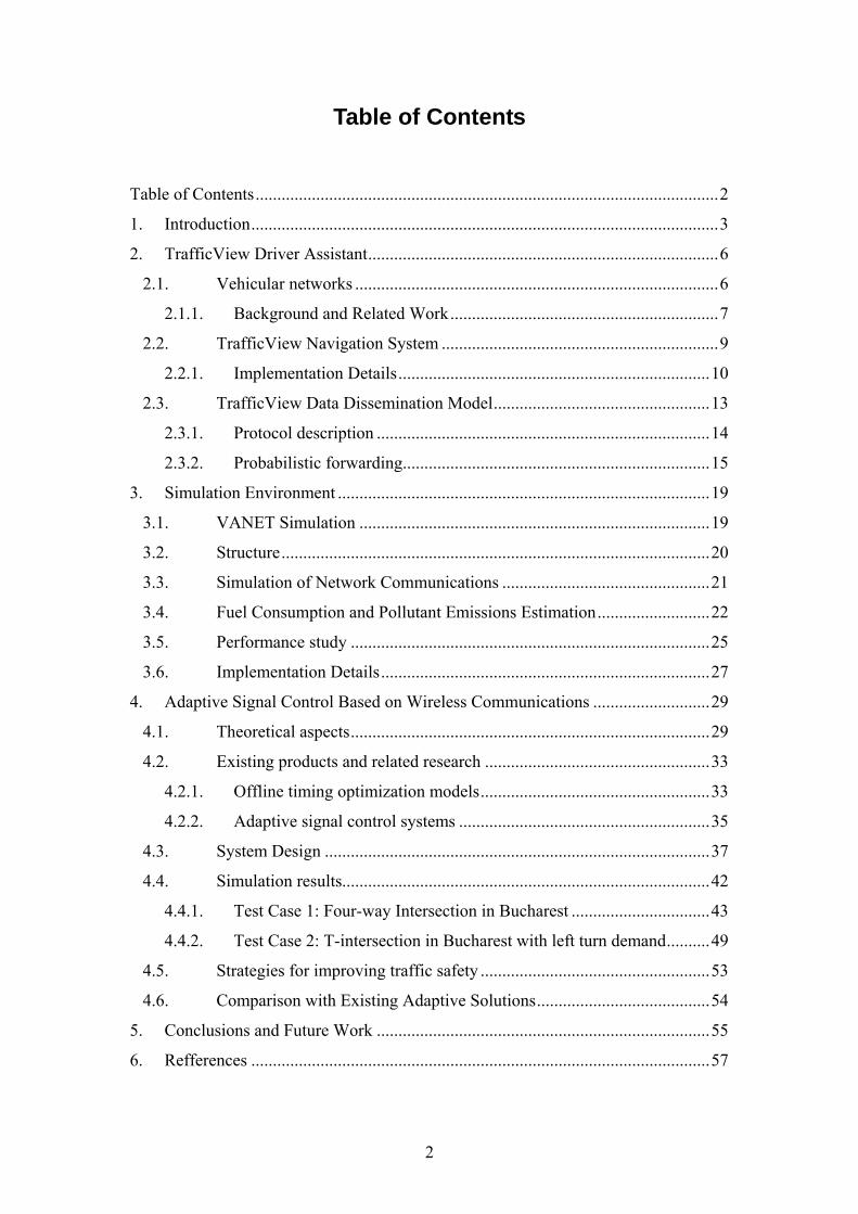
Table of Contents
Table of Contents...........................................................................................................2
1. Introduction............................................................................................................3
2. TrafficView Driver Assistant.................................................................................6
2.1. Vehicular networks ....................................................................................6
2.1.1. Background and Related Work..............................................................7
2.2. TrafficView Navigation System ................................................................9
2.2.1. Implementation Details........................................................................10
2.3. TrafficView Data Dissemination Model..................................................13
2.3.1. Protocol description .............................................................................14
2.3.2. Probabilistic forwarding.......................................................................15
3. Simulation Environment ......................................................................................19
3.1. VANET Simulation .................................................................................19
3.2. Structure...................................................................................................20
3.3. Simulation of Network Communications ................................................21
3.4. Fuel Consumption and Pollutant Emissions Estimation..........................22
3.5. Performance study ...................................................................................25
3.6. Implementation Details............................................................................27
4. Adaptive Signal Control Based on Wireless Communications ...........................29
4.1. Theoretical aspects...................................................................................29
4.2. Existing products and related research ....................................................33
4.2.1. Offline timing optimization models.....................................................33
4.2.2. Adaptive signal control systems ..........................................................35
4.3. System Design .........................................................................................37
4.4. Simulation results.....................................................................................42
4.4.1. Test Case 1: Four-way Intersection in Bucharest ................................43
4.4.2. Test Case 2: T-intersection in Bucharest with left turn demand..........49
4.5. Strategies for improving traffic safety .....................................................53
4.6. Comparison with Existing Adaptive Solutions........................................54
5. Conclusions and Future Work .............................................................................55
6. Refferences ..........................................................................................................57
2
1. Introduction Advances in mobile computing and wireless communication have offered new
possibilities for Intelligent Transportation Systems (ITS). Increasing interest has been
focused in the last years to deploy these technologies on vehicles and use them as a
means of improving driving safety and traffic efficiency.
By adding short-range communication capabilities to vehicles, the devices
form a mobile ad-hoc network, allowing cars to exchange information about road
conditions. This is often referred to in the literature as Vehicular Ad-hoc Networks
(VANETs) or Inter-Vehicular Communication (IVC) systems
The users of a VANET, drivers or passengers, can be provided with useful
information and with a wide range of interesting services. One category of such
services includes safety applications, like various types of warnings: ice on road,
intersection violation, cars in front braking, and collision avoidance and mitigation in
situations like: lane changing, lane merging and preparation for imminent collision.
Another important class of applications that can be deployed over VANETs is
concerned with traffic operations and maintenance: dynamic route planning, weather
conditions publishing and adaptive signal control in intersections. Commercial and
entertainment applications can be implemented as well, electronic payments,
reservations, advertisements or gaming and file transfer are just a few examples.
Thesis statement
This thesis examines the possibility of deploying an adaptive signal control
system in intersections, a system that can base its control decision on information
coming from cars. Thus, each intersection with traffic lights is provided with a
wireless infrastructure node that can extract data from an existing VANET.
For over thirty years now, efforts have been made to create traffic lights
systems that can respond to the ever increasing traffic. Most of the signal control
systems in United States, for example, are part of the first or the second generation,
3
and rely on timing plans generated offline by traffic engineers using optimization
models. These systems are hard to maintain and do not respond well to traffic events,
like a football game or road construction. More sophisticated adaptive traffic lights
use data coming from sensors, cameras and loop detectors to generate online timing
plans.
An architecture based on wireless communications can employ greater
flexibility than the ones mentioned before, providing more information for the signal
decision process. The cost is also significantly lower, considering loop detectors are
usually installed in the asphalt, under each lane approaching the intersections and
cameras require high processing power and good orientation.
Project Objectives
TrafficView is a data dissemination system we have implemented. It is an
application that runs on vehicles to collect and disseminate traffic information and
finally, to provide meaningful data to the driver. It is an example of a VANET
platform.
The adaptive signal control application presented here was developed to
communicate with TrafficView, a platform for inter-vehicle communication. The
main objectives are:
to increase the throughput and to decrease the average delay, considering
either one intersection or multiple coordinated intersections;
to reduce overall fuel consumption and emissions;
to increase safety in intersections.
Testing a VANET application is a real challenge because of the number of
nodes needed for a typical scenario and also because of the specific vehicle mobility
model. We have developed our own custom microscopic simulator that takes into
account this mobility model and simulates communication between nodes. With this
tool we have emulated the TrafficView application on hundreds and even thousands
of vehicles. We have also used the simulator to evaluate the adaptive traffic lights
system in various conditions and measure performance parameters.
4
The rest of this document is organized as follows. Section 2 provides a
description of the TrafficView, in the context of vehicular networks applications. A
general background and related research is discussed first, and then we present the
navigation system and data dissemination module in TrafficView. In Section 3 we
introduce an integrated VANET simulator with support for mobility, communication
between nodes and code emulation. Our adaptive traffic signal control mechanism,
based on communication with vehicles is presented in Section 4 and, finally, we draw
some conclusions in the final section.
5
2. TrafficView Driver Assistant
TrafficView is a data dissemination platform for VANETs that we have
implemented. It is an application that runs on vehicles to collect and disseminate
traffic information and finally, to provide meaningful information to the driver.
2.1. Vehicular networks
VANETs provide ITS with higher flexibility and scalability then systems that
rely on complex infrastructure deployed on the roadside. Because the devices are
installed in vehicles, some of the limitations of traditional mobile ad-hoc networks are
overcome. Thus, nodes are considered to have unlimited energy coming from the car
battery and there is enough space in a vehicle to install a computing device with good
processing power. However, the challenges a vehicular network faces are not few and
they may refer to rapid changes of the topology because of the high mobility of nodes,
to limitations of the wireless bandwidth or to frequent disconnections in the topology.
Improvements of this architecture, that could address some of these challenges, may
consider base stations or antennas being deployed in critical points along the roadside
or using occasionally WAN connectivity (like GPRS or 3G).
One important problem that deployment of car-to-car communication faces is
the fact that it is a technology with network effect: its value increases along with its
distribution. This makes it difficult to be deployed as the first users could not benefit
from car-to-car communication properly. Researchers have also been concerned with
the degrees of security such a vehicle network might need and possible ways to
achieve them. Having this in mind, electronic license plates seem like a possible node
authentication method. [4]
6
2.1.1. Background and Related Work
As it is an emerging technology, inter-vehicle communication is at the edge of
passing from academia and research laboratories to mass commercial production.
Although many car manufacturers have announced their intention of deploying this
feature on their future cars, relevant results may be found for now mostly in research
projects and simulations. Most of these projects try to make use of the collaborative
information exchange between vehicles in order to develop safety applications such as
emergency, traffic jam, traffic control, collision avoidance or obstacle warnings. A
routing protocol suitable for this highly mobile ad-hoc network is also needed in order
to provide multi-hop communication.
802.11 has been widely tested in inter-vehicular communication scenarios,
though it has a number of features that make it unfeasible for such an environment:
flexibility of radio resource assignment and of transmission rate control is low,
unlicensed frequency that produces interferences and a small signal range. There have
been numerous efforts to create wireless MAC protocols that are suitable for
VANETs. For example, Rao and Stoica suggest in [5] a layer on top of 802.11 MAC
layer that can solve asymmetric flow and hidden terminal issues.
In US, the Federal Communications Commission (FCC) has allocated 75 MHz
of spectrum at 5.9 MHz for Dedicated Short Range Communications (DSRC), a
variant of 802.11a [34]. Its goal is to support both safety applications and other
Intelligent Transportation System applications over roadside-to-vehicle and vehicle-
to-vehicle communication channels [15].
The FleetNet project, which ended in 2003, aimed to develop a
communication platform for inter-vehicle communication. The platform is suitable for
deploying three types of applications: cooperative driver assistance (emergency or
obstacle warning), decentralized floating car data (traffic jam monitor or dynamic
navigation) and user communication and user services (i.e. mobile advertising) [19].
For communication between vehicles the system uses UTRA TDD (UMTS Terrestrial
Radio Access Time Division Duplex) because of the availability of an unlicensed
frequency band at 2010–2020 MHz in Europe. As a routing protocol FleetNet chooses
7
a position-based protocol which is used along with a distributed location service and
relies on navigation systems.
The CarTalk 2000 project focuses its efforts on three application categories:
information and warning functions, communication-based longitudinal control
systems and co-operative assistance systems [9]. CarTALK, like FleetNet, uses the
UMTS radio access technology and also uses a position based routing protocol.
California PATH program has been engaged since 1986 in developing
solutions to transportation systems problems. Their work is focused on Policy and
Behavioral Research, Transportation Safety Research, Traffic Operations Research
and Transit Operations Research. Some of the many projects that are part of the
program envision inter-vehicle communication or vehicle-to-infrastructure
communication in systems ranging from safety messaging (using DSRC technology)
to automate driving, vehicle platoons formation and automated highways.
The fact that vehicle-to-vehicle and infrastructure-to-vehicle communication
are soon going to influence the way we drive is proved by recent news that show
important results coming from the automotive industry. DaimlerChrysler [37] have
publicly tested dynamic driving using wireless communication between cars in June
2005 using DSRC technology. Elsewhere, in Japan, Honda have announced the
completion of Honda ASV-3 Advanced Safety Vehicles equipped with cameras,
radars and communication devices providing new safety features like accidents
prevention, information about approaching obstacles and vehicles on the road or
drivers assistance in breaking and steering. [35].
For this technology to become ubiquitous there is an obvious need for
standardization in order to have compatibility between different car vendors. Efforts
are currently being made in Europe, Japan, US and other countries to accomplish this.
In Europe, the Car2Car Communication Consortium aims to promote the allocation of
a royalty free European wide exclusive frequency band for Car2Car applications and
to develop strategies and business models to speed-up the market penetration and
standardization.
8
2.2. TrafficView Navigation System
The TrafficView navigation module is in charge with efficient storage and
manipulation of the digital map, as well as accurate mapping of GPS readings to map
locations. As input for the maps we use the TIGER files available for free [13], in the
format of Record Type 1 (RT1) for and Record Type 2 (RT2). The two files types
permit us to construct the road graph. The RT1 files contain all the road segments for
a map region, with information like the type, name, direction, or starting and ending
points. The RT2 files contain intermediate points of the road segments for the
representation of curves. There are TIGER maps for every state in US, and for testing
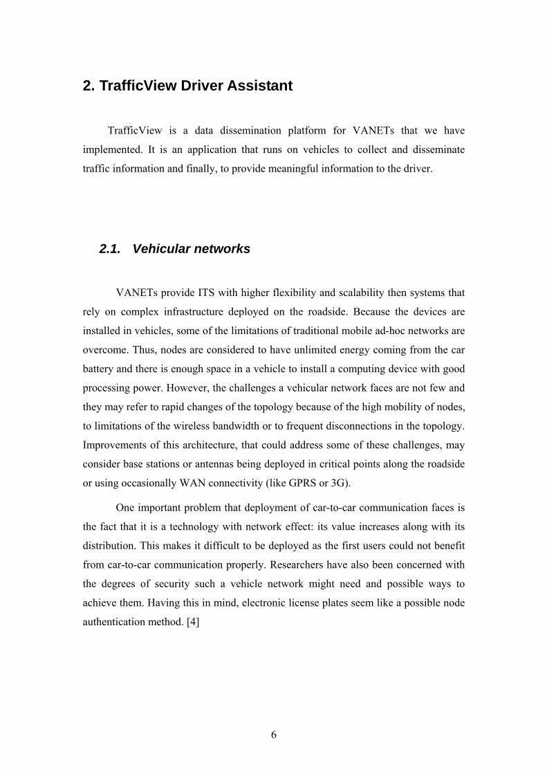
we have built our own, using the same format and representing a part of our campus
Figure 1. To calculate distances between points on the map we have used conversion
tables from degrees to meters depending on the latitude and longitude. The number of
meters per degree of latitude/longitude varies with the degree [14].
Figure 1 Dynamic map of the "Politehnica" University of Bucharest.
The geographical coordinates of a vehicle, read from the GPS device, are
transformed to a point on a road of the map and displayed accordingly to the driver. In
order to do this efficiently the system relies on the PeanoKey mechanism, initially
described in [1], which is efficient in terms of both search and storage.
A PeanoKey is associated with a point in the 2D space, and it is obtained by
interleaving the digits of the two coordinates. Thus, the 2D set of points is represented
in a one dimensional set. For example the PeanoKey associated with the geographical
9
point at 26.047800 degrees longitude and 44.435348 degrees latitude is
4246403457384080. When the map is being built, a set of sorted PeanoKeys is also
computed, corresponding to all the points of the map. Consecutive PeanoKeys in this
set correspond to points that are relatively close on the map.
Finding the closest point on the map, given the two GPS coordinates, latitude
and longitude, reduces first to finding the PeanoKey in the set that is the closest to the
PeanoKey newly formed and then, performing a linear local search around this
element.
2.2.1. Implementation Details
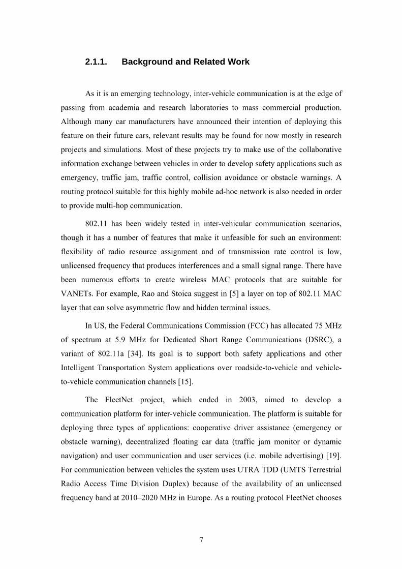
The first action taken when
TrafficView is started is to load the map into
an appropriate structure. The steps for this
task are summarized in Figure 2. First, the
Tiger RT1 file is parsed and a set of road
segments is built. This has, of course, an O(n)
complexity where n is the number of segments
in the .RT1 file. For each record in the .RT2
file, additional points are given for a specific
segment. This implies O(n2) complexity as for
each record, the corresponding segment has to
be located in the set, in order to add the points.
Although there may be multiple RT2 records
in the file for a single segment, only a part of
the segments are given records in the .RT2
file, namely the ones that have curves.
Load Intermediate Points
Merge Road Segments
Compute Point distances and PeanoKeys
Load Road Segments
Sort the PeanoKeys index
Compute crosses
Map Building Process
Figure 2. The sequence of actions for building the map structure.
10
The TIGER files contain points only for a few locations along a road
segments, such as curves or intersections. As we need to map a vehicle to a point on a
road more accurately, new points are created through interpolation. The points are
created with a specified resolution so no two consecutive points will be farther than a
configurable distance. This increases significantly the number of points, m, and
determines the complexity of the map building process.
The next phase takes care of merging the segments. The road segments in
.RT1 file are of small sizes and for a long road there may be tens of such records. This
makes them difficult to manipulate so they have to be merged. This step normally
takes O(n2) steps, because every two segments that have the same name have to be
considered.
For each point of the map, PeanoKey value is computed as specified above
along with a distance to the previous point on the segment it is on. The PeanoKey set
of all the points will be used for quick location finding and the distance value serves
for computing road distances between points.
Next, the PeanoKey set is sorted and this represents the most time expensive
step of the process: O(m log(m)) where m is the total number of points. Finally, given
the sorted set, finding the intersections between roads resumes to finding consecutive
equal values in this set, so it is only a O(m) traversal of PeanoKeys.
During the execution of the program, it is often needed to find the closest point
on the map, given the latitude and the longitude. This is accomplished by running a
binary search on the set of PeanoKeys (O(log(m)) complexity) and then the closes
point is found after a local linear search around the index returned by the binary
search.
Figure 3 presents the UML class diagram for the classes related to the map
structure. A map object has a collection of roads. Each road (Road.java) has a name,
number of lanes, a set of points and a set of crosses and it can be a one-way or two-
way street. Each point in the set of points of a road, has a longitude, latitude, distance
to the beginning of the segment and a reference to a PeanoKey value. All the
PeanoKey values are kept in a collection in the Map class. Likewise, each PeanoKey
has an inverse reference to a point on a road.
11
A road also has a set of crosses (Cross.java). Each cross object contains
references to the crossing segments and to the points of intersection.
Figure 3. The UML class diagram of the navigation module
12
2.3. TrafficView Data Dissemination Model
Most literatures suggest as a point of start to VANETs the application of
information dissemination between vehicles using periodical and regional broadcasts.
The main problem here is that broadcasts can result in flooding the network, also
known as the broadcast storm problem, so the number of messages has to be limited
in order to keep scalability. Several optimizations have been proposed, such as
decreasing the level of detail as the distance increases by using aggregation models
[1]. In [16], the authors present an adaptive way to set the broadcast period depending
on the significance of the message. In [17] several schemes (probabilistic, cluster
based and other) are proposed to reduce redundant rebroadcasts in wireless networks.
A configuration, in which information propagates through periodical
broadcasts from node to node, is said to work in the “push” mode. On the other side,
in the “pull” mode, information may be obtained on-demand, based on query-reply
communication. These two models may be put into balance when it comes to network
performance. In the “push” mode, increasing the range of the forwarding area results
in greater bandwidth requirements and more useless information. However, using
more queries even for shorter distances offers only the needed information but it is
less reliable and may increase the number of messages comparing to “push” mode as
the distances get shorter.
In TrafficView, vehicles periodically transmit information about themselves
and other cars on the road. They use one-hop broadcasts to avoid a broadcast storm
and each record consists of a position, identification number, speed, direction, state
and a timestamp of the moment when this information was created.
We have chosen to limit the size of the set of cars transmitted to fit in one
single packet. This avoids the delay caused by flow control which appears when
dealing with multiple packets. It also saves bandwidth and reduces the delay caused
by retransmissions.
Sets of car records are forwarded by each node alternatively, for cars running
on the same street and in the same direction with the forwarder, and for the opposite
direction (bi-directional model). Research shows that a propagation model that makes
use especially of the cars on the opposite direction when forwarding may have better
results in terms of distance of knowledge, error and delay of information. The bi-
13
directional model can adapt to situations when traffic on one direction is too low
switching to a single direction model.
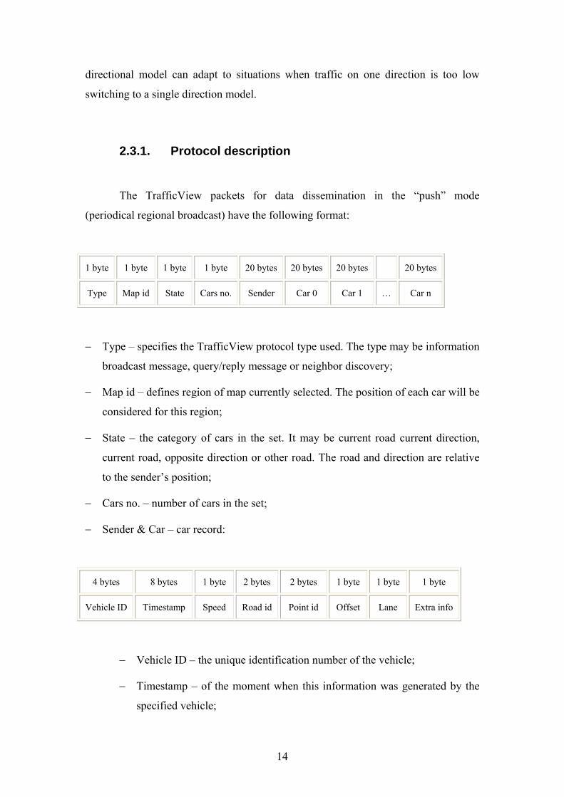
2.3.1. Protocol description
The TrafficView packets for data dissemination in the “push” mode
(periodical regional broadcast) have the following format:
1 byte 1 byte 1 byte 1 byte 20 bytes 20 bytes 20 bytes 20 bytes
Type Map id State Cars no. Sender Car 0 Car 1 … Car n
− Type – specifies the TrafficView protocol type used. The type may be information
broadcast message, query/reply message or neighbor discovery;
− Map id – defines region of map currently selected. The position of each car will be
considered for this region;
− State – the category of cars in the set. It may be current road current direction,
current road, opposite direction or other road. The road and direction are relative
to the sender’s position;
− Cars no. – number of cars in the set;
− Sender & Car – car record:
4 bytes 8 bytes 1 byte 2 bytes 2 bytes 1 byte 1 byte 1 byte
Vehicle ID Timestamp Speed Road id Point id Offset Lane Extra info
− Vehicle ID – the unique identification number of the vehicle;
− Timestamp – of the moment when this information was generated by the
specified vehicle;
14
− Speed – speed of the vehicle;
− Road & Point ids – specify the point on the map where that the car is the
closest to. We consider that vehicles have the same map format.
− Offset – distance to the map point;
− Lane – specifies the lane on which the car is running. This field is used
mostly in simulation, because current GPS systems are not that accurate.
− Extra information byte:
0 1 2 3 4 5 6 7
direction signal state
− Direction – the side of the road on which the car is running
− Signal – this field is the equivalent of the electrical signals of the
car and specifies the intentions of turning.
− State – the state of the car may be damaged, crashed or normal. The
state also gives information on the current transmission mode of
the car, such as active mode or promiscuous mode.
2.3.2. Probabilistic forwarding
Usually, on a highway or any other road, cars have a tendency to form
platoons. If every car uses the data dissemination model described above, redundant
information gets transmitted. This redundancy is even more obvious in a city
environment, where large groups of vehicles can be observed at intersections. For cars
that are moving along a street it is necessary that they broadcast their position, but
information about other cars may be redundant in the case of a platoon. In this case,
elimination of redundant information will not result in fewer messages (a moving ca
has to send minimum one record, itself), but it will result in smaller messages. Studies
of wireless networks [18] show the medium access and transmission delays vary
15
significantly depending on the packet size: from 5 milliseconds for 64 bytes, to 60
milliseconds for 2048 for a certain network load.
In TrafficView, we impose a scheme in which a vehicle functions in two
different modes: it either transmits a “keep alive” message with only one record with
its own data or a complete message with all the car records that it currently knows
about. At each broadcast period, the application will decide which type of message to
transmit in a probabilistic manner. It will transmit the full set of cars with a
probability proportional with the size, in meters, of the platoon that it is currently in.
For example, if two cars are very close to each other, it is a great chance that only one
will transmit the complete set of cars while if they are a few tens of meters apart
probably both will transmit the complete packet. In a wider and denser platoon, it is
ensured probabilistically that information (about cars in or outside the platoon) gets
transmitted from back to front and vice-versa without great redundancy.
The complete set of cars does not include car records that are older than a
certain threshold and it is limited to fit into one single Ethernet 802.11 frame of 2300
bytes.
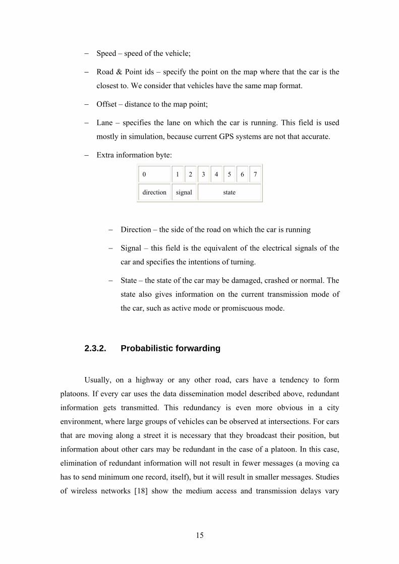
Figure 4 A view of the communication model used by each vehicle in a City Scenario (A) and a Highway Scenario (B). Vehicles are either in promiscuous mode (red), “keep alive” (orange) or complete forwarding
(blue).
In a city environment further optimizations can be accomplished by setting
cars that are not moving to promiscuous mode. However, such a car will warn the
surrounding nodes just before going into this state, in order not to be deleted from
their records when the entry would normally expire. As soon as the car starts moving,
it will switch back to normal mode. However, during the period a car is in
16
promiscuous mode, it may send complete messages if the probabilistic algorithm
decide it that it should.
In this way the number of messages exchanged in intersections or in congested
areas is greatly reduced and the performances of the network increase. Figure 4A
presents the network configurations in a city environment, near an intersection and on
a highway. In both pictures, the blue cars are the nodes that transmit messages with a
complete set of cars, while the orange ones send simple messages, informing only on
their position update. Furthermore, in Figure 4A, the vehicles that are stopped at the
traffic light, shown in red, are in promiscuous mode.
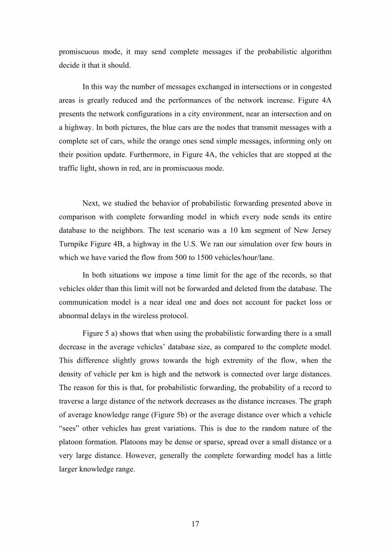
Next, we studied the behavior of probabilistic forwarding presented above in
comparison with complete forwarding model in which every node sends its entire
database to the neighbors. The test scenario was a 10 km segment of New Jersey
Turnpike Figure 4B, a highway in the U.S. We ran our simulation over few hours in
which we have varied the flow from 500 to 1500 vehicles/hour/lane.
In both situations we impose a time limit for the age of the records, so that
vehicles older than this limit will not be forwarded and deleted from the database. The
communication model is a near ideal one and does not account for packet loss or
abnormal delays in the wireless protocol.
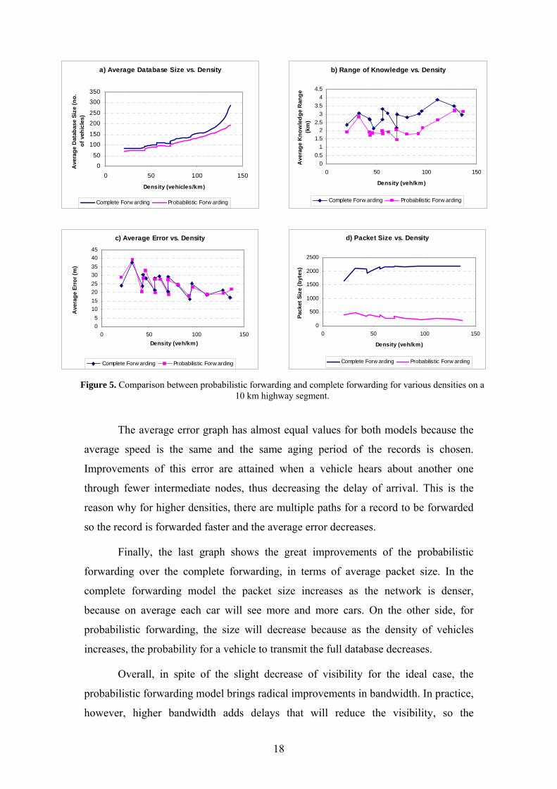
Figure 5 a) shows that when using the probabilistic forwarding there is a small
decrease in the average vehicles’ database size, as compared to the complete model.
This difference slightly grows towards the high extremity of the flow, when the
density of vehicle per km is high and the network is connected over large distances.
The reason for this is that, for probabilistic forwarding, the probability of a record to
traverse a large distance of the network decreases as the distance increases. The graph
of average knowledge range (Figure 5b) or the average distance over which a vehicle
“sees” other vehicles has great variations. This is due to the random nature of the
platoon formation. Platoons may be dense or sparse, spread over a small distance or a
very large distance. However, generally the complete forwarding model has a little
larger knowledge range.
17
a) Average Database Size vs. Density
050
100150
200250
300350
0 50 100 150
Density (vehicles/km)
Ave
rage
Dat
abas
e Si
ze (n
o.
of v
ehic
les)
Complete Forw arding Probabilistic Forw arding
b) Range of Knowledge vs. Density
00.5
11.5
22.5
33.5
44.5
0 50 100
Density (veh/km)
Ave
rage
Kno
wle
dge
Ran
ge
(km
)
150
Complete Forw arding Probabilistic Forw arding
c) Average Error vs. Density
05
1015202530354045
0 50 100 150Density (veh/km)
Ave
rage
Err
or (m
)
Complete Forw arding Probabilistic Forw arding
d) Packet Size vs. Density
0
500
1000
1500
2000
2500
0 50 100
Density (veh/km)
Pack
et S
ize
(byt
es)
150
Complete Forw arding Probabilistic Forw arding
Figure 5. Comparison between probabilistic forwarding and complete forwarding for various densities on a 10 km highway segment.
The average error graph has almost equal values for both models because the
average speed is the same and the same aging period of the records is chosen.
Improvements of this error are attained when a vehicle hears about another one
through fewer intermediate nodes, thus decreasing the delay of arrival. This is the
reason why for higher densities, there are multiple paths for a record to be forwarded
so the record is forwarded faster and the average error decreases.
Finally, the last graph shows the great improvements of the probabilistic
forwarding over the complete forwarding, in terms of average packet size. In the
complete forwarding model the packet size increases as the network is denser,
because on average each car will see more and more cars. On the other side, for
probabilistic forwarding, the size will decrease because as the density of vehicles
increases, the probability for a vehicle to transmit the full database decreases.
Overall, in spite of the slight decrease of visibility for the ideal case, the
probabilistic forwarding model brings radical improvements in bandwidth. In practice,
however, higher bandwidth adds delays that will reduce the visibility, so the
18
probabilistic forwarding model is expected to perform even better than the complete
forwarding model.
3. Simulation Environment
The evaluation of VANETs consists of real outdoor experiments, but also of
simulation and statistical analysis. The simulation process has to take into account
traffic conditions, driving characteristics and wireless communication protocols.
The VANET simulator we have developed is a discrete event simulator. The
simulation time advances with a fixed time resolution after executing the application
code for the current moment of the simulation time. More specifically, at every
moment of the simulation time, all the current events are pulled from a queue of
events, and handled in a random order.
3.1. VANET Simulation
Network simulators, like NS-2 or GloMoSim, implement the full network
protocol stack and simulate the signal propagation model and the physical
environment for wireless communications. For IVC, wireless network simulators have
to take into account the mobility of nodes that can affect signal propagation.
Traffic simulators can be microscopic or macroscopic. Microscopic simulators
model local behavior of individual vehicles by representing the velocity and position
of each vehicle at a given moment. Macroscopic simulators model traffic condition in
a global manner and may use concepts from wave theory. Usually traffic is
represented in terms of flows (vehicle/hour), density (vehicles/km) or average speed.
In relation to IVC, microscopic simulation offers a more relevant
representation. CORSIM [36] or VISSIM [38] are examples of microscopic traffic
simulators that models vehicle interactions, traffic flows, congestions or streets and
intersections geometry.
19
Considering the way they are built, simulation environments can be time based
or event based. In time based models, like meteorological or traffic simulators, time
advances with a fixed quantum and the entities act accordingly. Event based
simulators (network simulators) increase time variably, based on the occurrence of
events.
3.2. Structure
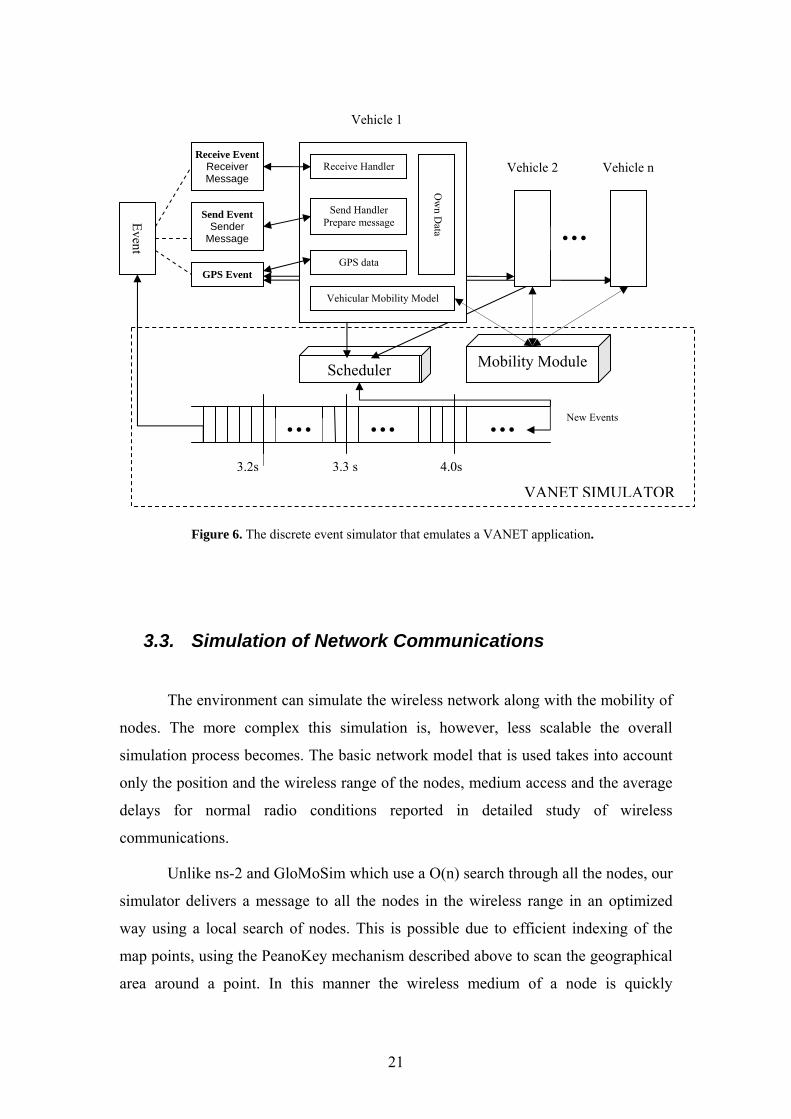
The events queue can hold three types of events: send, receive or GPS. A send
event for a specified node triggers the calling of the node’s procedure responsible for
preparing a message. It also schedules the corresponding receive event(s) for the
receiver(s) the simulator decides to deliver the message to, according to the network
module. The receive event is associated either with a node, or with a group of nodes
(broadcast) and it calls the appropriate handler in each of the receiving nodes. The
GPS event is scheduled at a regular time interval for each node, in order to simulate
the way a real VANET application collects GPS data periodically.
Besides these three types of events, the mobility module updates periodically
the position of each node that is a vehicle, according to the vehicular mobility model.
This model takes into account vehicle interactions (passing by, car following patterns
etc), traffic rules and various driver behavior.
The main advantage of this architecture is that the simulator can execute (or
emulate) the real application’s code without significant changes. Practically, we have
succeeded to simulate the TrafficView application [1] on each node, by calling the
appropriate methods of the application when the corresponding events occur. Some
minor changes were in order, because the original application was multithreaded
which would be a serious limitation for the simulator. Figure 1 shows the top-down
view of this simulation environment.
20
Scheduler
3.2s 4.0s3.3 s
Mobility Module
Vehicular Mobility Model
Receive Handler
Send Handler Prepare message
GPS data
Ow
n Data
Vehicle 1
Vehicle 2 Vehicle n
● ● ● ● ● ● ● ● ●
Event
Receive Event Receiver Message
● ● ●
Send Event Sender
Message
GPS Event
New Events
VANET SIMULATOR
Figure 6. The discrete event simulator that emulates a VANET application.
3.3. Simulation of Network Communications
The environment can simulate the wireless network along with the mobility of
nodes. The more complex this simulation is, however, less scalable the overall
simulation process becomes. The basic network model that is used takes into account
only the position and the wireless range of the nodes, medium access and the average
delays for normal radio conditions reported in detailed study of wireless
communications.
Unlike ns-2 and GloMoSim which use a O(n) search through all the nodes, our
simulator delivers a message to all the nodes in the wireless range in an optimized
way using a local search of nodes. This is possible due to efficient indexing of the
map points, using the PeanoKey mechanism described above to scan the geographical
area around a point. In this manner the wireless medium of a node is quickly
21
analyzed, its wireless neighbors are discovered and a map of the radio signal is built
in order to assure medium access.
To have a more accurate network model, more factors need to be taken into
account. The node’s protocol stack is one of these factors and the simulator can have
the packet encapsulation process simulated by adding all the corresponding headers to
the messages being sent. As a transport layer, UDP is preferred, while the IP network
layer can be replaced by a geographical routing and addressing scheme. The MAC
layer is 802.11b. The signal propagation model takes into account signal fading, gain
or loss caused by collisions or interference with other radio devices.
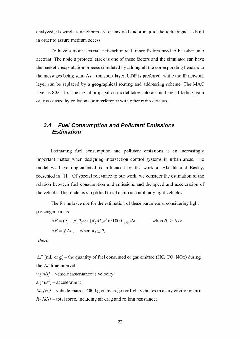
3.4. Fuel Consumption and Pollutant Emissions Estimation
Estimating fuel consumption and pollutant emissions is an increasingly
important matter when designing intersection control systems in urban areas. The
model we have implemented is influenced by the work of Akcelik and Besley,
presented in [11]. Of special relevance to our work, we consider the estimation of the
relation between fuel consumption and emissions and the speed and acceleration of
the vehicle. The model is simplified to take into account only light vehicles.
The formula we use for the estimation of these parameters, considering light
passenger cars is:
, when RtvaMvRfF avTi Δ++=Δ > )]1000/[( 02
21 ββ T > 0 or
, when RtfF iΔ=Δ T ≤ 0,
where
FΔ [mL or g] – the quantity of fuel consumed or gas emitted (HC, CO, NOx) during
the time interval; tΔ
v [m/s] – vehicle instantaneous velocity;
a [m/s2] – acceleration;
Mv [kg] – vehicle mass (1400 kg on average for light vehicles in a city environment);
RT [kN] – total force, including air drag and rolling resistance;
22

adrrvT FFaMR ++⋅=
rrF - rolling resistance force:
gMCF vrrrr ⋅⋅= , (for each tire)
Crr – rolling resistance coefficient, 0.15 on average for each tire
(depends on road surface)
adF - air drag force:
dad CAvF ⋅⋅⋅⋅= 2
21 ρ
ρ - air density (1.29 kg/m3)
A – frontal car area (2.1 m2 on average for light vehicles)
Cd – drag coefficient (0.3 for a car)
if [mL/s or g/s] – idle fuel consumption rate or gas emissions rate;
1β [mL or g per kJ] – fuel consumed or gas emitted per engine energy unit;
2β [mL or g per (kJ⋅m/s2)] – coefficient for fuel consumption or gas emissions per
unit of energy-acceleration, reflects the function behavior on positive acceleration.
The values of the last three parameters are given in the following table. They
are based on the work reported by Akcelik and Besley, presented in [11].
fi β1 β2
Fuel consumption 1350 [mL/s] 900 [mL/kJ] 300 [mL/(kJ⋅m/s2)]
CO 50 [g/s] 150 [g/kJ] 250 [g/(kJ⋅m/s2)]
HC 8 [g/s] 0 [g/kJ] 4 [g/(kJ⋅m/s2)]
NOx 2 [g/s] 10 [g/kJ] 2 [g/(kJ⋅m/s2)]
The CO2 is calculated based on the fuel consumed:
2)()( 2 COffuelFCOF ⋅Δ=Δ ,
where is the CO2COf 2 emission rate given in grams per milliliter of fuel [g/mL].
2COf = 2.5 g/mL for light vehicles
23
Speed vs Time
-20
0
20
40
60
80
100
0 10 20 30 40 50 60
Time (s)
Spe
ed (k
m/h
)
Acceleration vs Time
-6
-4
-2
0
2
4
0 10 20 30 40 50 60
Time (s)
Acce
lera
tion
(m/s
2 )
Fuel Consumption vs Time
0
10
20
30
40
50
0 10 20 30 40 50 60
Time (s)
Fuel
Con
sum
ptio
n (L
/h)
Figure 7 Example of fuel consumption estimation for a vehicle that passes through an intersection
24
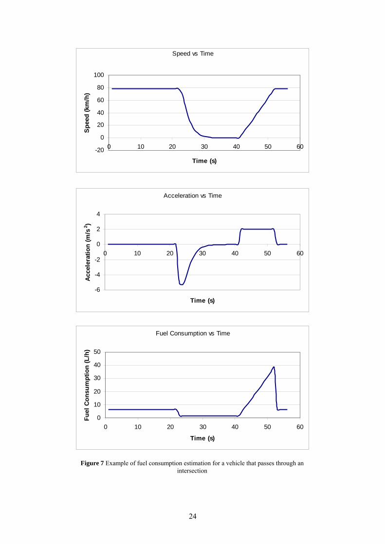
3.5. Performance study
As described above, three main parts can be distinguished in the simulation
process: mobility, simulator engine and emulation of the nodes’ application.
Optionally, the simulation may run with a graphical user interface we have
implemented, but additional time is consumed with display functions and the
synchronization mechanisms. The mobility model works as a micro-simulator. It
consumes time on moving each car independently, considering all the nearby cars that
may affect it and the traffic rules that apply. The simulator engine manages the events
queue and establishes communication between nodes. Each time a node sends a
message, the engine searches for all the cars in the node’s wireless range to deliver the
message. It performs a linear search on a limited set of elements around the
geographical position of the node, using the PeanoKey mechanism described in the
previous sections.
0
50100
150200
250
300350
400
21.5
26.1
29.3
33.8
38.4
43.7
48.3 54 58
.765
.871
.7
Density (vehicles / km)
Seco
nds
need
ed to
sim
ulat
e 5
min
utes
of t
he s
cena
rio
GUI (s)Code (s)Mobility (s)Events (s)
Figure 8 Time measurements for the simulation process and its components, depending on the density
of vehicles. Test scenario: 10 km of highway with a traffic flows varying between 500 and 1500 vehicles/hour/lane.
The most time consuming part of the simulation is code emulation (Figure 3).
The TrafficView application, which functions on each node, has to parse all the
incoming messages, update the local vehicle records and create new messages for
broadcast. Figure 8 shows that for high densities, when the network is widely
25
connected, messages are propagated easily from car to car and more than half of the
simulation time goes on processing the messages received by each of them.
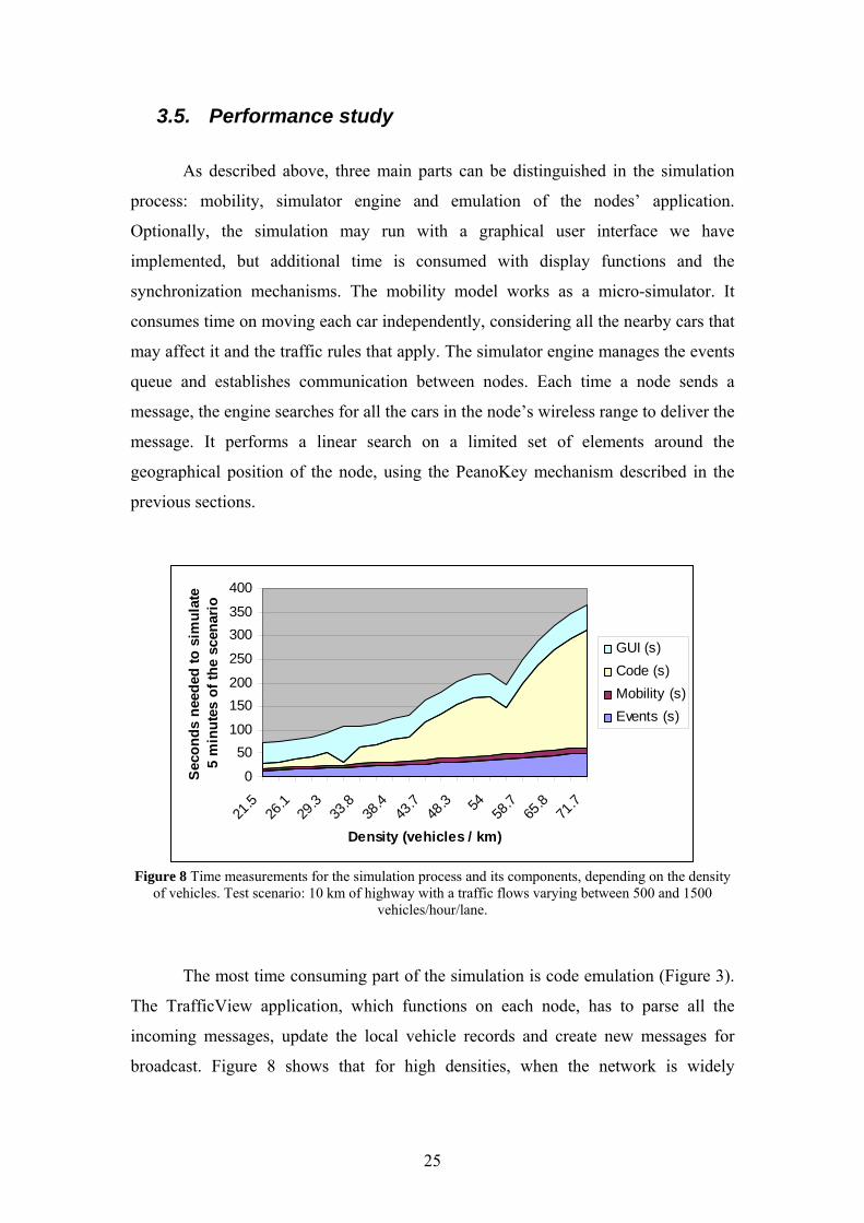
Figure 9. UML class diagram of the simulator engine module (JAVA)
26
3.6. Implementation Details
The UML class diagram in Figure 9 shows the core structure of the simulator
written in Java. The main class, Engine, manages the nodes of the network and the
interactions between them, which are triggered by events. The GUI and the
communication between nodes can be switched off for particular studies or
improvements in performance.
Each car node of the network is represented by the SimulatedCarInfo class
which extends the class CarInfo, which contains basic data needed for representing
the car such as vehicle id, speed, latitude, longitude, direction, timestamp and a few
others. The timestamp is the time when the GPS device of that car got the data. The
class SimulatedCarInfo adds the methods that come with the TrafficView application
that runs on each node. The class also implements the Communicator interface which
contains the methods for needed for a node to communicate with the network. The
map is loaded into memory only once, as a global object, and all the entities in the
simulator may have access to the map structure. The methods that are called whenever
the state of a node needs to change are basically three:
− SimulatedCarInfo.update() – is called periodically, when the node’s new
position and speed are read from the GPS. The role of the GPS is
simulated by the mobility module which moves the vehicles on the map;
− SimulatedCarInfo.prepareMessage() – is called when the node is supposed
to send a message previously scheduled, either as a periodical or single
message.
− SimulatedCarInfo.receive() – is called when a node receives a message
from another node. The engine decided that the node received this
message, based on its position and the message protocol address.
Each of these methods is called whenever the specific event occurs in the
engine. They are handlers that the engine knows to call when appropriate.
When the engine advances the simulation time, it pulls out from the main
event queue that it manages all the events for the new moment of time. The Event
class holds a time variable, for the moment when it will occur. This class is extended
by classes representing particular types of events that add more information; for
example, the Receive event has 2 communicators (a sender and a receiver) and the
27
array of bytes that form the message. The SendEvent class is used for broadcasts, and
it is extended by UnicastSendEvent for one hop unicasts. The CleanupEvent is used to
when the cars need to cleanup their databases of old records. It replaces a cleanup
thread in the real TrafficView application.
The network also permits communication between nodes, other than cars, such
as infrastructure nodes. The WirelessTrafficLight class, used to implement the logic
described in the following section, also implements the Communicator interface, has a
geographical position and may communicate with the other nodes.
Finally, the engine receives input from the emissions and fuel consumption
module that is connected to the mobility model. Each time a car is moved on the map,
its speed an acceleration determine an estimation of the fuel consumption and
pollutant emission as previously described.
28
4. Adaptive Signal Control Based on Wireless Communications
For over thirty years now, efforts have been made to create traffic lights
systems that can respond to the ever increasing traffic. A first step in adapting traffic
lights to the traffic demand was signal timing according to the time of the day. This
solution is based on signal plans generated offline by traffic engineers and requires
consistent maintenance effort as traffic changes. A possible improvement represents
the use of input from sensors to select a signal plan that best suits the situation and
modify it online. A limitation of this strategy is encountered in situations where
events that influence traffic often occur, like touristic regions or intersections near
stadiums or malls. Fully adaptive or fully actuated traffic signals generate timing
plans online, based on input from sensors that measure traffic parameters.
This thesis examines the possibility of implementing an adaptive traffic light
system, based on wireless communication with the vehicles. It proposes the use of
network infrastructure nodes that can benefit from the information exchange in
TrafficView and get a clear real-time view of the traffic.
In the following section we will present the basic theoretical aspects that are
taken into account when designing signal control systems. Then, a brief history and
the current achievements in the field are discussed. In section 4.2 the design of
TrafficView Signal Control system is described. Finally we will present the
simulation tests cases we have run and the results we have obtained when using our
system.
4.1. Theoretical aspects
A timing plan for a signal control at an intersection is specified through three
parameters: cycle length, green splits and offsets. The cycle length is the time it takes
for a traffic light to pass through all its phases before it repeats the first phase. The
split of each phase is the duration of the phase expressed in percentage of the cycle
29
length. The offset is the difference between the start times of green periods at two
adjacent intersections and is used for coordination between traffic lights.
There are several goals that can be taken into consideration when designing a
signal control mechanism [6]:
minimizing the average delay of vehicles approaching an intersection
increasing progression, by coordinating vehicle platoons between
intersections
reducing the queue length of all approaches to an intersection
maximizing overall throughput, by analyzing traffic at the intersection,
arterial or network level
Achieving two or more of these goals may be contradictory. For example,
increasing progression may not be the optimum for minimizing total delay, because
traffic on arterials is encouraged at the expense of congesting minor approaches.
However, we will consider the main measure of effectiveness (MOE) for an
intersection is the control delay, which is the component of the intersection delay
caused by the presence of the signal control [30]. It is measured in comparison with
the travel time calculated in the absence of a control mechanism. Another relevant
parameter is v/c or volume per capacity ratio which reflects the degree of saturation of
an approach to the intersection. For saturated intersections the degree of saturation is
calculated through the demand per capacity ratio which is greater than 1. The queue
length, calculated in number of cars, might also be an important parameter that would
help analyze the geometrical configuration of the intersection and detect downstream
congestions. Downstream congestions are traffic jams that occur immediately after
passing through an intersection, possibly caused by the queue at the next intersection.
This process seriously affects the traffic flow, or even freezes it, and may be also
referred to as starvation.
Minimizing the delay at intersections, suggests the selection of a cycle length
as short as possible, in order to produce less red time and shorter queues. The intuition
here is that the cycle length should be shortened until a critical value is reached, a
30
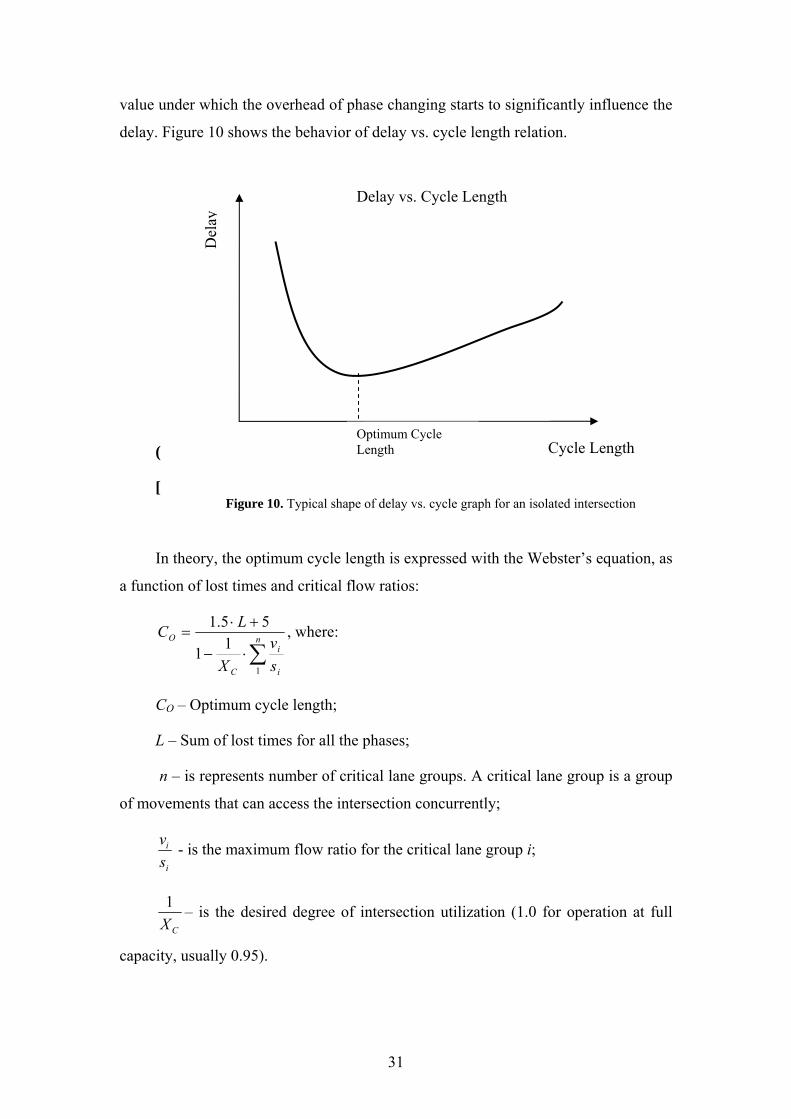
value under which the overhead of phase changing starts to significantly influence the
delay. Figure 10 shows the behavior of delay vs. cycle length relation.
(
Delay vs. Cycle Length
[
In theory, the optimum cycle length is expressed with the Webster’s equation, as
a function of lost times and critical flow ratios:
∑⋅−
+⋅= n
i
i
C
O
sv
X
LC
1
11
55.1 , where:
O – Optimum cycle length;
– Sum of lost times for all the phases;
– is represents number of critical lane groups. A critical lane group is a group
of movements that can access the intersection concurrently;
C
L
n
i
i
sv - is the maximum flow ratio for the critical lane group i;
CX1 – is the desired degree of intersection utilization (1.0 for operation at full
capacity, usually 0.95).
Cycle Length
Del
ay
Optimum Cycle Length
Figure 10. Typical shape of delay vs. cycle graph for an isolated intersection
31
The lost time is calculated as the sum of inter-green periods. The inter-green
perio e and all-red time, and represents the
interval when usually no car enters the intersection. For an intersection with
pedes
T al flow of the lane
group, for which the timing is considered, per saturation flow. The saturation flow is
calculated
signal would be green for an hour. A typical value for the saturation flow is 1900
e, but there are several factors that can reduce this value, such
as narr
ping. The intersections
can be
ebster’s formula presented above, the global cycle
length
d for a phase is the sum of yellow tim
trian crossings, the sum of green time and inter-green time for one phase has to
be long enough to permit pedestrians to safely cross the street.
he flow ratio for a lane group is computed as the actu
as the maximum number of vehicles that can enter the intersection, if the
vehicles per hour per lan
ow lanes, large number of turning movements, or large number of trucks and
busses.
In city environments, coordination between multiple intersections along
arterials is crucial. The goal of traffic lights coordination is to have large platoons of
vehicles move through a sequence of intersections without stop
best coordinated when they are uniformly spaced. Too great distances between
signals can cause the cars in platoons to spread, thus reducing the effect of
coordination.
Coordination of the traffic signals in a sequence of intersections means setting
an equal cycle length for all the signals. For optimum results this cycle length is
chosen by analyzing the critical intersection in the sequence, the one with the
maximum flow. Considering W
will be equal to the maximum of the optimum cycle length for each signal
along the path. If the cycle length of a signal differs significantly from the remaining
intersection, than it can function in using double or half of the value selected for the
other signals.
32
4.2. Existing products and related research
The evolution of traffic signal control systems is divided into three generations:
First Generation – The signal control systems in this category use pre-
calculated signal plans, generated offline, that are selected based on time of
the day. The plans change every 15 minutes and the devices are non-
computerized.
Second Generation – These systems choose online the signal plans, based on
surveillance data and predicted values. Optimization of timing plans may
ited to 10 minutes.
at may implement
system that achieves coordination.
system
plans f
is onlin
sensors
There are several software tools on the market, which are used in cities all over
the world to create tim
that implements a, so called, mesoscopic
traffic model for the analysis and optimizations of intersections and network of
tersections. A mesoscopic traffic model estimates at each moment of the simulation
occur every 5 minutes but choosing new plans is lim
Usually the data is processed by a central computer th
coordination between intersections.
Third Generation – Fully responsive traffic control systems that also rely on
sensors, but can change the plans more rapidly (3-5 minutes). These systems
are more independent, having their own processing module, and may be part
of a distributed
Thus, there are two different strategies to creating suitable signal control
s. The first alternative is using offline optimization models that generate signal
or intersections based on simulations or input parameters. The other alternative
e adaptive control systems that implement signal plans based on data from
, running their algorithms online.
4.2.1. Offline timing optimization models
ing plans based on input traffic measurements. The output of
these tools is used by traffic engineers to pre-set the traffic lights. Following we
describe the models behind the most important of these tools.
TRANSYT is a software program
in
33
the traf tha hat stop at red lights,
or the number of vehicle that depart on green or the platoon formation along a street.
The
hes through all possible
cycle
SYNCHRO is a tool that is widely accepted in USA and used to optimize
inters
The optimization process has several stages. Like TRANSYT it analyzes all
cycle
steps: first with 4-second increments, then 2-second and finally 1 second.
For coordination between two adjacent intersections SYNCHRO calculates a factor
reflec
mostly on coordination [6]
fic flow t enters each segment, the number of vehicles t
optimization techniques TRANSYT uses try to reduce the total delay and the
number of stops of a network of intersections. This are the main MOE (measures of
effectiveness) this tool analyzes for the generated traffic flows.
In the signal optimization process, TRANSYT first searc
lengths, and analyzes each value in order to find the best results. For each cycle
length it computes the green splits that produce equal saturation degrees on all
approaches. The splits are further optimized by searching the best solution around
these values, also taking into account offsets between adjacent signals [21].
The latest version uses genetic algorithms to find the most suitable sequence of
phases.
ections all over the world. Its philosophy is to minimize a performance indicator
that is a function of delay, number of stops and queue length. The traffic model used
is similar to the model of TRANSYT. SYNCHRO analyses a group of intersection
limited to 10 for the simple version and to 300 for the distributed one [20].
lengths in a specified domain. The offsets and splits are optimized using a
search in
ting the extent to which they can be coordinated, based on link distance, travel
times and volume.
PASSER II and V are similar optimization tools that uses a genetic algorithm
to find the best timing plans at several intersections along an arterial so they focus
34
4.2.2. Adaptive signal control systems
Several adaptive traffic control systems have been implemented for intersections
all over the world. The most important ones include Split, Cycle and Offset
Optimization Technique (SCOOT) [24], Sydney Coordinated Adaptive Traffic
System (SCATS) [22], Los Angeles Adaptive Traffic Control System (LA-ATCS),
ptimized Policies for Adaptive Control (OPAC) and Real-time Hierarchical
ptimized Distributed and Effective System (RHODES) [23].
SCOOT [24] is the most widely used, with hundreds of installation worldwide.
It is ba loo ersection, usually at the
upstream end of the approach. Thus, based on the actual field demand, SCOOT
creat
ee optimization stages:
Split Optimizer, Offset Optimizer and Cycle Optimizer. They work in small
increm
predicted delays and stops for the approach
nated intersections. A critical intersection
is ide
O
O
sed on p detectors placed on every link to an int
es Cyclic Flow Profile (CFP) and models platoon movements, queue formation
and discharge. To measure demand, it uses LPUs (Link Profile Units), a fundamental
measure of flow and occupancy.
The optimization process takes place at central location, where all the data from
the monitored intersections arrive, and then timing plans are adjusted and sent back to
the traffic lights controllers in the intersections. There are thr
ents that are evaluated according to a performance index, a function of
ing vehicles. The Split Optimizer runs at
each phase change and analyzes how the modification of the current phase with up to
4 seconds (in any way) would influence performance. The Offset Optimizer runs once
per cycle and based on CFPs predicted for adjacent nodes may decide modifications
of the offset also with up to 4 seconds. The Cycle Optimizer runs periodically, every
five minutes, considering a group of coordi
ntified in the group, and then an optimum cycle is calculated for a saturation
degree of 90%. The old cycle is modified with up to 16 seconds towards the new
calculated cycle.
For incident detection SCOOT has two special modules. ASTRID (Automatic
SCOOT Traffic Information Database) is a system that offers historical information
like daily flow profiles and expected congestion levels. INGRID or Integrated
35
Incident Detection is a module that detects unusual events in the traffic that affect
traffic. It looks for sudden changes in flow and occupancy on a link or important
deviations from the historical data. Incidents are indicated when there is significant
decrease in flow and occupancy at the downstream detector.
Other systems, like SCATS, have detectors placed immediately before the stop
line at an intersection. Thus, it cannot get accurate data when the queue grows beyond
the length of the detector, or the link is over saturated. Since it uses a model based
espec
inally runs intersection
optimizations algorithms. The detectors are usually placed 200-300 feet upstream the
intersection, which may also represent a limitation for longer queues.
error more appropriate for automated driving the human drivers.
Coor
ially on occupancy, it also has difficulties in differentiating between high flows
or intersection stoppage. Reported research shows poor performance when incidents
occur. [25]
RHODES suggests a hierarchical architecture of the control system. At the
highest level it predicts traffic flows at the vehicle and platoon resolution level. Then,
it allocates green based on various demand patterns and f
The problem of intersections management as a cooperation problem in a
distributed network has been intensively studied. Dresner and Stone propose a
reservation-based multiagent control policy for a simplified traffic model, which
allows car to schedule their intersection access [26]. However, their system assumes
margins of
dinating traffic signals, which are agents in a distributed environment, has also
been implemented using evolutionary game theory techniques [28] or other self
organizing methods [27].
36
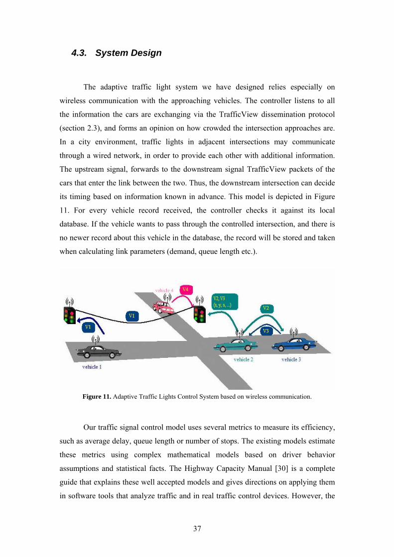
4.3. System Design
The adaptive traffic light system we have designed relies especially on
s communication with the approaching vehicles. The controller listens to all
ation the cars are exchanging via the TrafficView dissemination protocol
(section 2.3), and forms an opinion on how crowded the intersection approaches are.
a city environment, traffic lights in adjacent intersections may communicate
rough a wired network, in order to provide each other with additional information.
he upstream signal, forwards to the downstream signal TrafficView packets of the
cars that enter the link between the two. Thus, the downstream intersection can decide
ing based on information known in advance. This model is depicted in Figure
11. For every vehicle record received, the controller checks it against its local
atabase. If the vehicle wants to pass through the controlled intersection, and there is
about this vehicle in the database, the record will be stored and taken
Our traffic signal control model uses several metrics to measure its efficiency,
such as average delay, queue length or number of stops. The existing models estimate
these metrics using complex mathematical models based on driver behavior
assumptions and statistical facts. The Highway Capacity Manual [30] is a complete
guide that explains these well accepted models and gives directions on applying them
in software tools that analyze traffic and in real traffic control devices. However, the
wireles
the inform
In
th
T
its tim
d
no newer record
when calculating link parameters (demand, queue length etc.).
Figure 11. Adaptive Traffic Lights Control System based on wireless communication.
37
real situations are very complex and traffic conditions depend on a large number of
the
moment the simulator determines a car to be influenced by the traffic light
from the traffic
of analysis (the
value greater than 95 % of the set).
The
capacity r
saturation
link. The volume is the traffic flow measured at the point where the cars enter the
variables so estimation models can sometimes have significant errors.
Our control method benefits from the wireless communication system with
vehicles and can measure accurately traffic metrics. Next we describe the most
important metrics we use and how are they computed by the system:
Control delay – is calculated for each car that passes through an
intersection. As mentioned in section 4.1 it is the difference between the
travel time that would have occurred in the absence of the intersection
control, and the travel time reported by a vehicle, in the presence of the
intersection control. At the simulator level the delay is calculated from
either directly or indirectly through other cars that are slowing down. At
the controller application level, as it would be the case of a real device, this
delay is calculated from the moment the car and the controller agree that
the car has been influenced by the signal. The average delay over an
analysis period is the main measurement of effectiveness.
Queue length – is computed by the traffic controller, who knows the
traffic configuration at every moment. To find the end of the queue, it has
to check the database, and advance form car to car starting
light, until a gap larger than threshold or a vehicle speed higher than a
threshold is encountered. The queue length value is saved at every 10
seconds and offered in the 95th percentile form for a period
The number of stops – is calculated for each car that passes through the
intersection; the traffic light knows the vehicle’s queuing time and pass
through time so it can compute the number of stops based on the timing
history.
way the controller takes its timing decision is based on the volume per
atio, as described in section 4.1. It is important when calculating the
degree of a link to differentiate between the volume and the demand of the
38
intersection
upstream o mber of cars
that de e
described i
end of the
at the stop
queue whil
Ou
they are i ntersection, so it is able to measure
accurat
of connect
informatio
The plan generation process takes place once, during each cycle and
stablishes a plan for the following cycle based on the measured parameters. During a
cycle, further optimizations may occur, such as phase skipping, phase extension or
interruption. The tim
. On the other hand, the demand is the traffic flow measured at a point
f any queue that forms at the intersection, and reflects the nu
sir to pass through the intersection. For example, SCOOT, the system
n section 4.2.2, measures demand by placing the detectors at the upstream
link and estimates the volume. In contrast, SCATS has the detectors placed
line, before entering an intersection, and calculates the volume and the
e it estimates the approach demand.
r system maintains contact with the vehicles throughout the entire period
n a few miles range around the i
ely both volume and demand. Due to the fact that, on a road, there may be gaps
ivity between vehicles, the system may rely when measuring the demand on
n sent by the adjacent traffic signal over a wired network.
timing
e
ing generation procedure has two stages:
a. Phase sequence selection
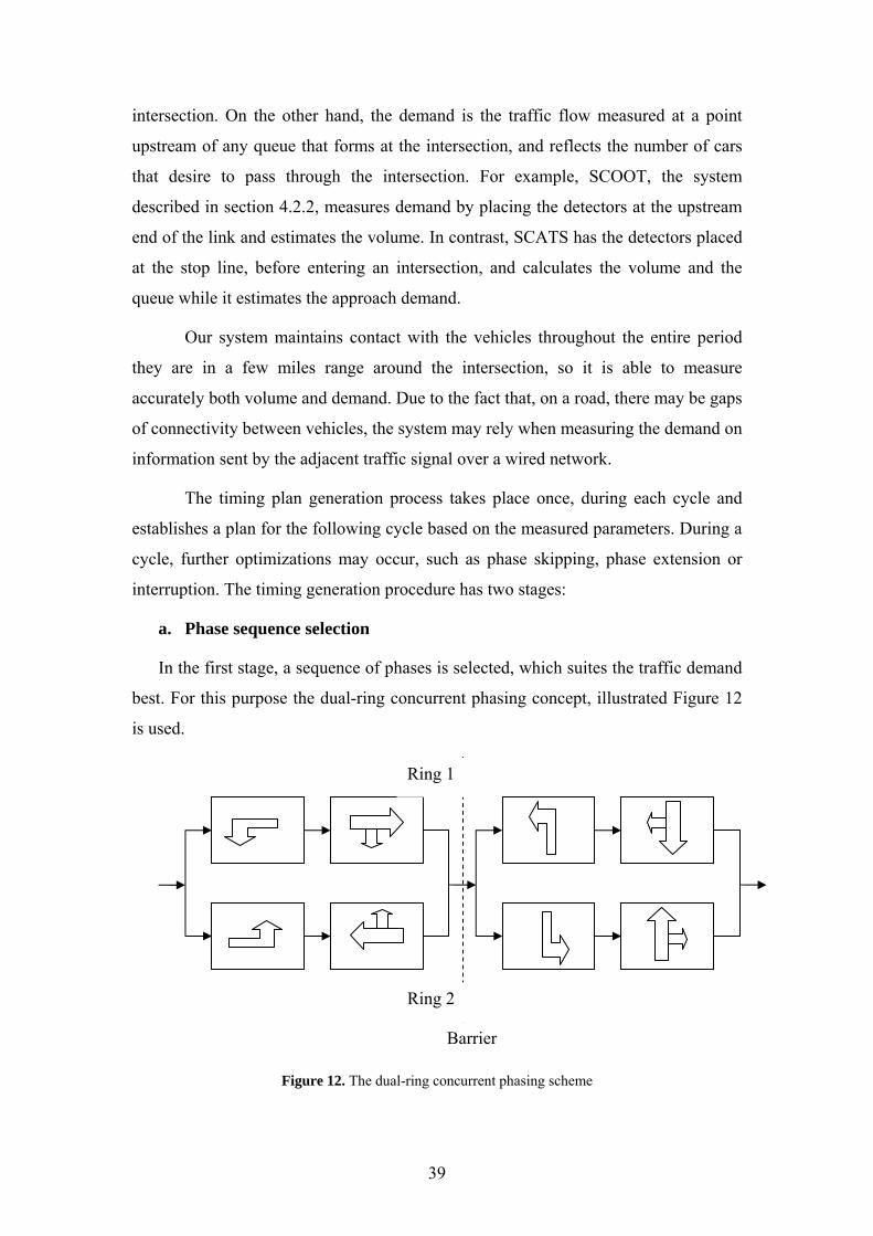
In the first stage, a sequence of phases is selected, which suites the traffic demand
best. For this purpose the dual-ring concurrent phasing concept, illustrated Figure 12
is used.
Ring 1
Barrier
Ring 2
Figure 12. The dual-ring concurrent phasing scheme
39
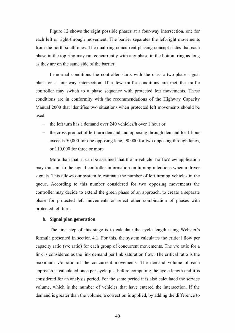
Figure 12 shows the eight possible phases at a four-way intersection, one for
each left or right-through movement. The barrier separates the left-right movements
from al-ring concurrent phasing concept states that each
phase in the top ring may run concurrently with any phase in the bottom ring as long
as they are o
normal conditions the controller starts with the classic two-phase signal
plan for a four-way intersection. If a few traffic conditions are met the traffic
controller may switch to a phase sequence with protected left movements. These
conditions are in conformity with the recommendations of the Highway Capacity
Manual 2000 that identifies two situations when protected left movements should be
used:
− the left turn has a demand over 240 vehicles/h over 1 hour or
− the cross product of left turn demand and opposing through demand for 1 hour
exceeds 50,000 for one opposing lane, 90,000 for two opposing through lanes,
or 110,000 for three or more
More than that, it can be assumed that the in-vehicle TrafficView application
may transmit to the signal controller information on turning intentions when a driver
This allows ou vehicles in the
queue. According to this number considered for two opposing movements the
control
lated once per cycle just before computing the cycle length and it is
considered for an analysis period. For the same period it is also calculated the service
volume, which is the num rsection. If the
demand is greater than the volume, a correction is applied, by adding the difference to
the north-south ones. The du
n the same side of the barrier.
In
signals. r system to estimate the number of left turning
ler may decide to extend the green phase of an approach, to create a separate
phase for protected left movements or select other combination of phases with
protected left turn.
b. Signal plan generation
The first step of this stage is to calculate the cycle length using Webster’s
formula presented in section 4.1. For this, the system calculates the critical flow per
capacity ratio (v/c ratio) for each group of concurrent movements. The v/c ratio for a
link is considered as the link demand per link saturation flow. The critical ratio is the
maximum v/c ratio of the concurrent movements. The demand volume of each
approach is calcu
ber of vehicles that have entered the inte
40
the m
in the a
en splits for each phase are allocated to produce
equal d
de and. This correction represents the number of cars that did not manage to pass
nalyzed period so they have to be counted for the demand for the next period
Having a cycle length, the gre
egrees of saturation on each link. The formula that is used here is:
∑⋅−=
j
j
i
i
i
sv
sv
LCG )( ,
where Gi is the green time for phase i, C is the cycle length, L the total lost time
during a cycle (yellow and all red times), and vi/si the critical volume per capacity
rati i.
e
control
movement,
that cause the formation of a queue on the left lane, that may influence and cause
delays on the right-through movements as well. In this situation the green phase for
the approach with the left lane queue will be extended to allow protected left turns and
discharge the queue.
o for the movements in phase
This preliminary signal plan is adjusted to meet various limitations such as a
maximum cycle length or pedestrian minimum green time. The green time for
pedestrians is usually calculated considering the average pedestrian speed of 4 ft/s, the
road width and a minimum WALK light time before the last pedestrian starts crossing
the road.
After the minimum green time for an approach has passed, which allowed
pedestrians to cross the conflicting approach(es), the phase may be interrupted if no
incoming vehicles are detected. On the other side, if the green phase for an approach
has finished, but cars keep coming while there is no demand on the conflicting
approach(es) the green phase may be extended until an acceptable pedestrians waiting
time. Another special event that may occur at the end of a green phase is when th
ler detects left turning vehicles with unusual waiting times, comparing to the
through movement. This may be because of high volumes on the opposing
41
Finally, after the new signal timing plan has been developed, the traffic light
may broadcast feedback messages for the incoming cars. These messages give
information on when the phase will switch and how large the queue is on each lane of
every approach. Feedback messages have several purposes:
1. They regulate the incoming traffic on an approach because in-vehicle
and speed of a vehicle greatly influence the fuel consumed
(Figure 7)
4.4
ts we have obtained when
using our system
ran hundred
wireless adaptive solution m
to the existing solutio
software can recommend appropriate speeds based on when the current
phase will end, and how many cars are already queued. This has an
obvious beneficial impact on safety as drivers know precisely if they can
pass or not on the current phase.
2. Delay in intersection is reduced because the drivers know in advance when
the phase changes and they can act accordingly (either avoid decelerating
too much on red or react faster on green).
3. Fuel consumption and pollutant emissions are reduced. In the situations
when the vehicles aren’t forced to stop because the drivers know they will
catch a green light, less acceleration occurs. It is known that the
acceleration
. Simulation results
In this section we present the test cases and the resul
. For testing, we have used the simulator described in section 3 and
s of hours of simulation for each scenario. The results show that the
anaged to perform better in all the cases, when comparing
ns.
42
4.4.1. Test Case 1: Four-way Intersection in Bucharest
first test scenario we evaluate is the intersection Iuliu Maniu / Vasile
Bucharest.
The
Milea in We will study the operations at this intersection without
onsidering the effect of adjacent intersections. We will focus on comparing two types
f signal control strategies: pre-timed fixed signal control as it currently is and an
adaptive strategy based on communication between the controller and approaching
eh hicles equipped with wireless communication
evices.
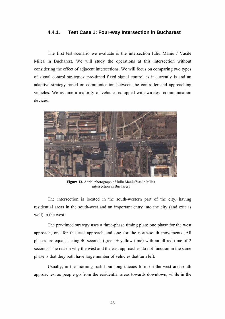
The intersection is located in the south-western part of the city, having
residential areas in the south-west and an important entry into the city (and exit as
well) to the west.
The pre-timed strategy uses a three-phase timing plan: one phase for the west
approach, one for the east approach and one for the north-south movements. All
phases are equal, lasting 40 seconds (green + yellow time) with an all-red time of 2
seconds. The reason why the west and the east approaches do not function in the same
phase is that they both have large number of vehicles that turn left.
Usually, in the morning rush hour long queues form on the west and south
approaches, as people go from the residential areas towards downtown, while in the
c
o
v icles. We assume a majority of ve
d
Figure 13. Aerial photograph of Iuliu Maniu/Vasile Milea intersection in Bucharest
43
after-no h the
ast-west flows are due to vehicles that are entering or exiting the city.
on. Usually, on the
northbound and eastbound approaches
long
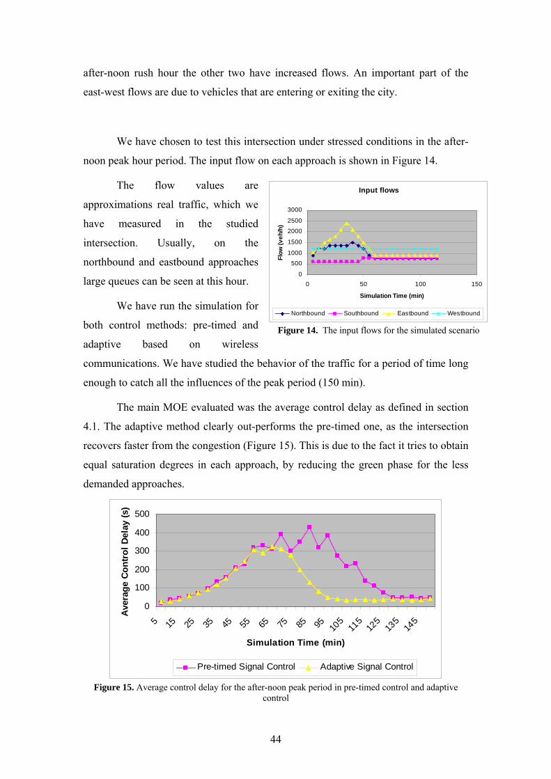
enough to catch all the influences of the peak period (150 min).
The main MOE evaluated was the average control delay as defined in s tion
4.1. The adaptive method clearly out-performs the pre-timed one, as the intersection
covers faster fro ct it tries to obtain
qual saturation degrees in each approach, by reducing the green phase for the less
mand
on rush our the other two have increased flows. An important part of
e
We have chosen to test this intersection under stressed conditions in the after-
noon peak hour period. The input flow on each approach is shown in Figure 14.
The flow values are
approximations real traffic, which we
have measured in the studied
intersecti
large queues can be seen at this hour.
We have run the simulation for
both control methods: pre-timed and
adaptive based on wireless
communications. We have studied the behavior of the traffic for a period of tim
Input flows
2000
2500
3000
/h)
0
5001000
1500
0 50 100 150
Simulation Time (min)
Flow
(veh
Northbound Southbound Eastbound Westbound
Figure 14. The input flows for the simulate ario d scen
e
ec
re m the congestion (Figure 15). This is due to the fa
e
de ed approaches.
400
500
lay
(s)
0
100
200
300
5 15 25 35 45 55 514
565 75 85 95 105
115
125
13
Aver
age
Cont
rol D
e
Simulation Time (min)
Pre-timed Signal Control Adaptive Signal Control
Figure 15. Average control delay for the after-noon peak period in pre-timed control and adaptive control
44
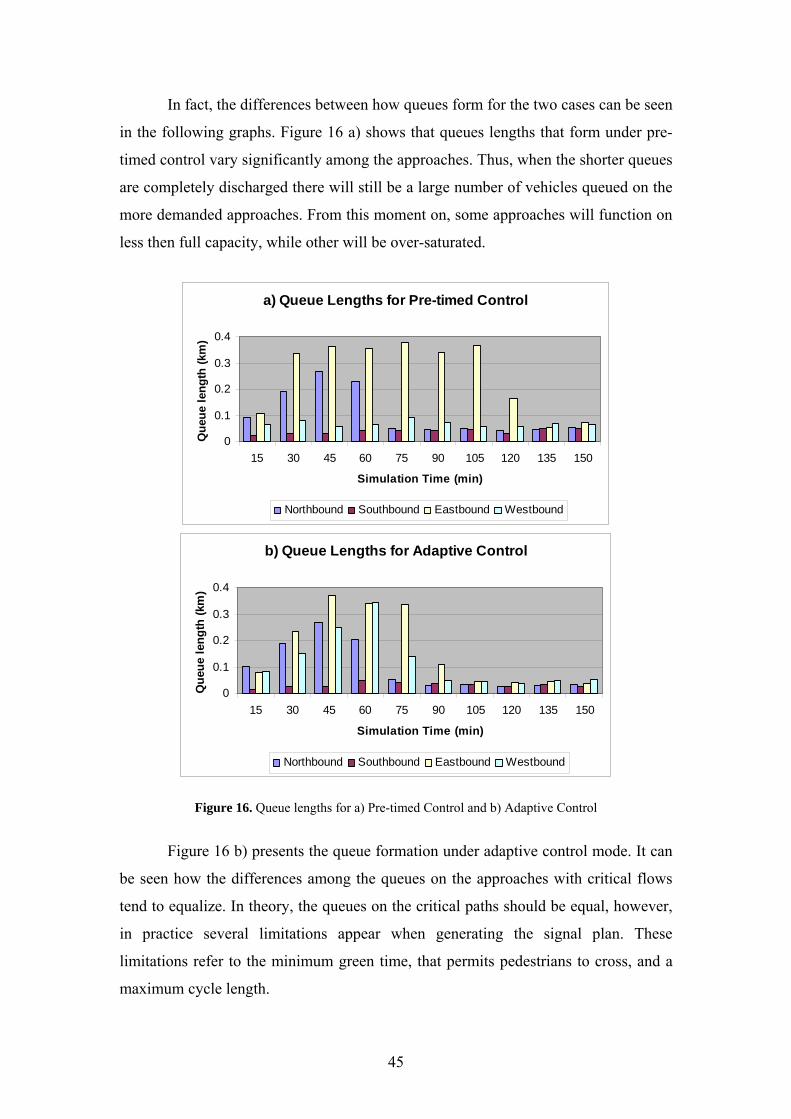
In fact, the differences between how queues form for the two cases can be seen
in the following graphs. Figure 16 a) shows that queues lengths that form under pre-
med control vary significantly among the approaches. Thus, when the shorter queues
are completely discharged there will still be a large number of vehicles queued on the
ti
more demanded approaches. From this moment on, some approaches will function on
less then full capacity, while other will be over-saturated.
a) Queue Lengths
0.1
0.2
0.3
0.4
e le
ngth
(km
)
for Pre-timed Control
015 30 45 60
Sim
Qu
75 90 105 120 135 150
ula
eu
tion Time (min)
Northbound Southbound Eastbound Westbound
b) Queue Lengths for Adaptive Control
0
0.1
0.2
0.3
0.4
Que
ue le
ngth
(km
)
15 30 45 60 75 90 105 120 135 150
Simulation Time (min)
Northbound Southbound Eastbound Westbound
Figure 16. Queue lengths for a) Pre-timed Control and b) Adaptive Control
Figure 16 b) presents the queue formation under adaptive control mode. It can
be seen how the differences among the queues on the approaches with critical flows
tend to equalize. In theory, the queues on the critical paths should be equal, however,
in practice several limitations appear when generating the signal plan. These
limitations refer to the minimum green time, that permits pedestrians to cross, and a
maximum cycle length.
45
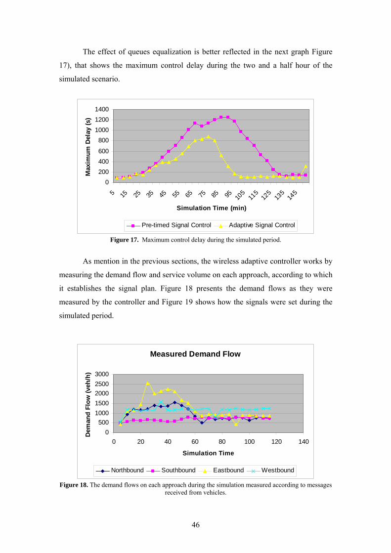
The effect of queues equalization is better reflected in the next graph Figure
17), that shows the maximum control delay during the two and a half hour of the
simulated scenario.
0200400600
800100012001400
(s)
5 15 25 35 45 55 65 75 85 95 105
115
125
135
145
Simulation Time (min)
Max
imum
Del
ay
Pre-timed Signal Control Adaptive Signal Control
Figure 17. Maximum control delay during the simulated period.
As mention in the previous sections, the wireless adaptive controller works by
measuring the demand flow and service volume on each approach, according to which
it establishes the signal plan. Figure 18 presents the demand flows as they were
measured by the controller and Figure 19 shows how the signals were set during the
simulated period.
Measured Demand Flow
0500
0 20 40 60 80 100 120 140
Simulation Time
Dem
a
1000
2025003000
nd F
low
(veh
/h)
150000
Northbound Southbound Eastbound Westbound
Figure 18. The demand flows on each approach during the simulation measured according to messages received from vehicles.
46
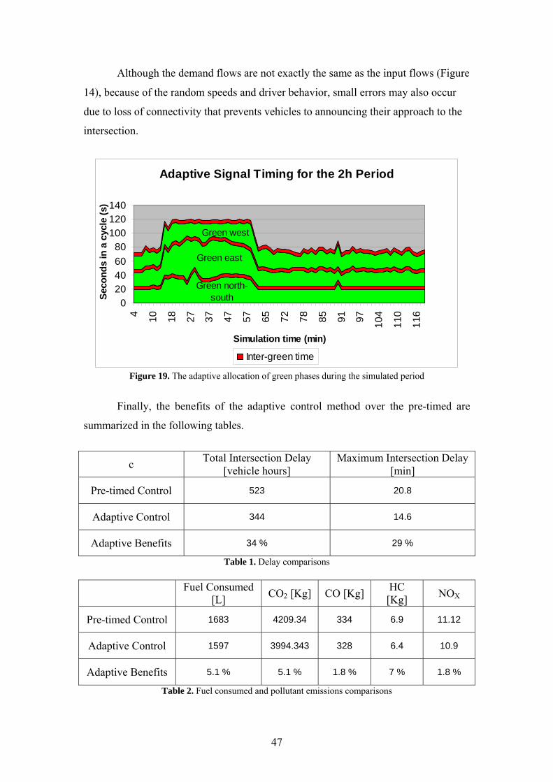
Although the demand flows are not exactly the same as the input flows (Figure
14), because of the random speeds and driver behavior, small errors may also occur
due to loss of connectivity that prevents vehicles to announcing their approach to the
tersection.
in
Adaptive Signal Timing for the 2h Period
Green north-south
Green east
Green west
020406080
100120140
4 10 18 27 37 47 57 65 72 78 85 91 97 104
110
116
Seco
nds
in a
cyc
le (s
)
Simulation time (min)
Inter-green time
Figure 19. The adaptive allocation of green phases during the simulated period
Finally, the benefits of the adaptive control method over the pre-timed are
summarized in the following tables.
c Total Intersection Delay [vehicle hours]
Maximum Intersection Delay [min]
Pre-timed Control 523 20.8
Adaptive Control 344 14.6
Adaptive Benefits 34 % 29 %
Table 1. Delay comparisons
Fuel Consumed [L] CO2 [Kg] CO [Kg] HC
[Kg] NOX
Pre-timed Control 1683 4209.34 334 6.9 11.12
Adaptive Control 1597 3994.343 328 6.4 10.9
Adaptive Benefits 5.1 % 5.1 % 1.8 % 7 % 1.8 %
Table 2. Fuel consumed and pollutant emissions comparisons
47

as
od are expected to be even more important for less congested scenarios.
It must be taken into consideration that this analysis was done in a worst-case
scenario of a congested intersection. It is assumed that the pre-timed signal plan w
developed by the authorities especially for this scenario. Therefore, the benefits of the
adaptive meth
48
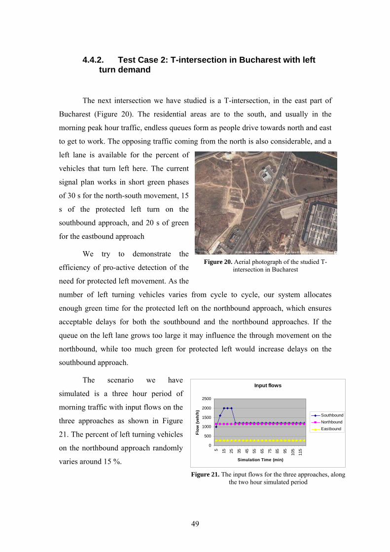
4.4.2. Test Case 2: T-intersection in Bucharest with left turn demand
The next intersection we have studied is a T-intersection, in the east part of
ucharest (Figure 20). The residential areas are to the south, and usually in the
morning peak hour traffic, endless queues form as people drive towards north and east
to get to work. The opposing traffic coming from the north is also considerable, and a
left lane is available for the percent of
vehicles that turn left here. The current
signal plan works in short green phases
of 30 s for the north-south movement, 15
s of the protected left turn on the
southbound approach, and 20 s of green
for the eastbound approach
We try to demonstrate the
efficiency of pro-active detection of the
need for protected left movement. As the
number of left turning vehicles varies from cycle to cycle, our system allocates
enough green time for the protected left on the northbound approach, which ensures
acceptable delays for both the southbound and the northbound approaches. If the
queue on the left lane grows too large it may influence the through movement on the
northbound, while too much green for protected left would increase delays on the
southbound approach.
The scenario we have
simulated is a three hour period of
morning traffic with input flows on the
three approaches as shown in Figure
21. The percent of left turning vehicles
on the northbound approach randomly
varies around 15 %.
B
Figure 20. Aerial photograph of the studied T-intersection in Bucharest
Input flows
0
500
1000
1500
2000
2500
5 15 25 35 45 55 65 75 85 95 105
115
Simulation Time (min)
Flow
(veh
/h)
SouthboundNorthboundEastbound
Figure 21. The input flows for the three approaches, along the two hour simulated period
49
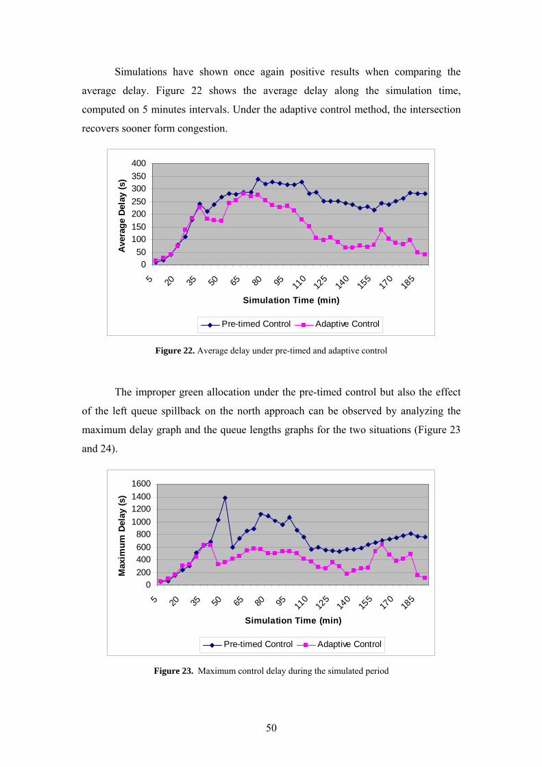
Simulations have shown once again positive results when comparing the
average me,
omputed on 5 minutes intervals. Under the adaptive control method, the intersection
recovers sooner form congestion.
delay. Figure 22 shows the average delay along the simulation ti
c
050
100150200250300350400
5 20 35 50 65 80
Simu
Aver
age
Del
ay (s
)
95 110
125
140
155
170
185
lation Time (min)
Pre-timed Control Adaptive Control
re-timed and adaptive control
er the pre-timed control but also the effect
Figure 22. Average delay under p
The improper green allocation und
of the left queue spillback on the north approach can be observed by analyzing the
maximum delay graph and the queue lengths graphs for the two situations (Figure 23
and 24).
120014001600
y (s
)
0200400600800
1000
5 20 35 50 65 80
Sim
Max
imum
Del
95 110
125
140
155
170
185
ulation Time (min)
a
Pre-timed Control Adaptive Control
he simulated period Figure 23. Maximum control delay during t
50
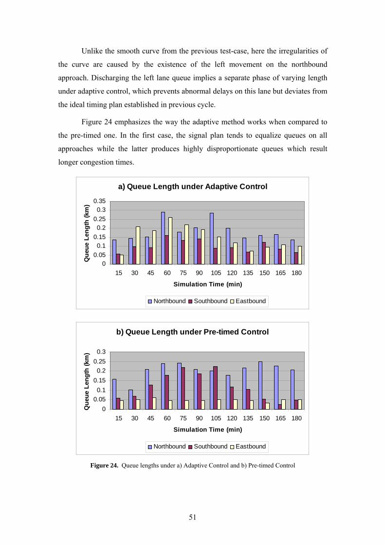
Unlike the smooth curve from the previous test-case, here the irregularities of
the curve are caused by the existence of the left movement on the northbound
approach. Discharging the left lane queue implies a separate phase of varying length
under adaptive control, which prevents abnormal delays on this lane but deviates from
the ideal timing plan established in previous cycle.
Figure 24 emphasizes the way the adaptive method works when compared to
the pre-timed one. In the first case, the signal plan tends to equalize queues on all
approaches while the latter produces highly disproportionate queues which result
longer congestion times.
a) Queue Length under Adaptive Control
00.050.1
0.150.2
0.250.3
0.35
15 30 45 60 75 90 105 120 135 150 165 180
Simulation Time (min)
Que
ue L
engt
h (k
m)
Northbound Southbound Eastbound
b) Queue Length under Pre-timed Control
00.050.1
0.150.2
0.250.3
15 30 45 60 75 90 105 120 135 150 165 180
Simulation Time (min)
Que
ue L
engt
h (k
m)
Northbound Southbound Eastbound
Figure 24. Queue lengths under a) Adaptive Control and b) Pre-timed Control
51
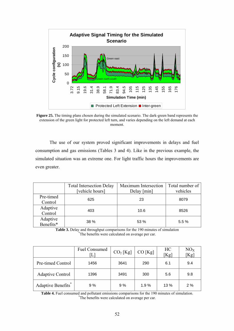
Adaptive Signal Timing for the Simulated Scenario
Green east
100
150
200
igur
atio
n (s
)
Green north-south
0
503.
72
9.15
19.6
31.4
38.9
58.1
71.9
83.4
94.5
105
115
125
135
145
155
165
176
Cyc
l
Simulation Time (min)
e co
nf
Protected Left Extension Inter-green
Figure 25. The timing plans chosen during the simulated scenario. The dark-green band represents the extension of the green light for protected left turn, and varies depending on the left demand at each
moment.
The use of our system proved significant improvements in delays and fuel
consumption and gas emissions (Tables 3 and 4). Like in the previous example, the
simulated situation was an extreme one. For light traffic hours the improvements are
even greater.
Total Intersection Delay [vehicle hours]
Maximum Intersection Delay [min]
Total number of vehicles
Pre-timed Control 625 23 8079
Adaptive Control 403 10.6 8526
Adaptive Benefits* 38 % 53 % 5.5 %
Table 3. Delay and throughput comparisons for the 190 minutes of simulation *The benefits were calculated on average per car.
Fuel Consumed [L] CO2 [Kg] CO [Kg] HC
[Kg] NOX[Kg]
Pre-timed Control 1456 3641 290 6.1 9.4
Adaptive Control 1396 3491 300 5.6 9.8
Adaptive 2 % Benefits* 9 % 9 % 1.9 % 13 %
Table 4. Fuel consumed and pollutant emissions comparisons for the 190 minutes of simulation. *The benefits were calculated on average per car.
52
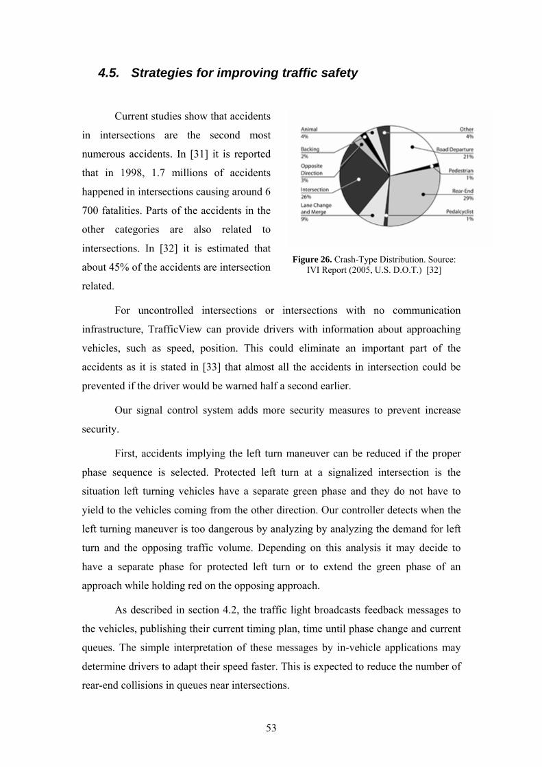
4.5. Strategies for improving traffic safety
Current studies show that accidents
in intersections are the second most
numerous accidents. In [31] it is reported
that in 1998, 1.7 millions of accidents
happened in intersections causing around 6
700 fatalities. Parts of the accidents in the
other categories are also related to
intersections. In [32] it is estimated that
rela
about 45% of the accidents are intersection
ted.
Figure 26. Crash-Type Distribution. S urce:
For uncontrolled intersections or intersections with no communication
e driver would be warned half a second earlier.
Our signal control system adds more security measures to prevent increase
security.
accidents implying the left turn maneuver can be reduced if the proper
phase sequence is selected. Protected left turn at a signalized intersection is the
situation lef turning vehicles have a separate green phase and they do not have to
yield to the vehicles coming from the other direction. ontroller detec the
lef
turn and the opposing traffic volume. Depending on this analysis it may decide to
ave a separate phase for protected left turn or to extend the green phase of an
approach while holdin os h
in sec .2, the tra ht bro ts feed messages to
t hing the rent timing plan, time until phase change and current
queues. The simple interpretation of these messages by in-vehicle applications may
adapt their speed faster is ex to red e num f
rea
oIVI Report (2005, U.S. D.O.T.) [32]
infrastructure, TrafficView can provide drivers with information about approaching
vehicles, such as speed, position. This could eliminate an important part of the
accidents as it is stated in [33] that almost all the accidents in intersection could be
prevented if th
First,
t
Our c ts when
t turning maneuver is too dangerous by analyzing by analyzing the demand for left
h
g red e oppon th ing approac .
As described tion 4 ffic lig adcas back
he vehicles, publis ir cur
determine drivers to . This pected uce th ber o
r-end collisions in queues near intersections.
53
w crossings that cause
violent crashes in intersections. When the wireless controller detects such situations it
extends n is cleared.
g Adaptive Solutions
control based on wireless communication
s based on sensors. Its strength is that
re information to the decision process. It
the
to loop detectors, for example that detect only flow and occupancy. Its
th is also its weakness, as it requ
traffic demand.
ughout the entire period they
Another safety measure can be taken for red or late yello
the all-red phase until the intersectio
4.6. Comparison with Existin
Conceptually speaking, the adaptive
is different in its design from the one that i
communicating with the vehicles implies mo
may benefit from knowing the position,
opposed
speed and the driver’s intention, as
streng ires vehicles to have GPS and wireless
communication devices and run software that publishes private data. Existing adaptive
solutions function independently of the cars by using sensors and cameras. However,
the two technologies do not exclude each other as they may work together. It is
important to identify the benefits each solution brings.
A first perspective to look at the functionality differences is the method of
detecting
The solutions that rely on loop detectors have to set the detectors at a fixed
location upstream the intersection. This raises questions about where is the best place
for installing them. If the detector is placed too close to the intersection and the queue
grows beyond this point the demand volume cannot be estimated and it is limited to
the service volume (vehicles that pass on each green phase). If the detector is placed
too far on a link and there are vehicles that exit or enter the link along this distance,
the flow measured is inaccurate.
However, our system monitors the vehicles thro
are in the area of the intersection. The only limitation is when a queue grows that
much that the dissemination model fails to propagate information from the back of the
queue to the front. This is because the maximum packet size limitation described in
section 3. This limitation can be eliminated by installing additional antennas along the
road.
54
An important advantage our system has over existing solutions is that drivers
can send their movement intentions in advance. This makes the control method more
responsive. For example, the pro-active detection of left turning demand is an
ffective measure of reducing total delay and increasing security. Current solutions
can accomplish this only through video image analysis which has several limitations.
Cam nd require
creased computational power, and they can detect only the cases when there is a
larger q
into consideration is that a
solution based on wireless communication needs an adequate wireless protocol.
DSRC
applications with wireless communication.
ation in a probabilistic manner is evaluated
in com
Ts. The simulator is discrete event oriented and has support for the complex
e
eras have to be pointed towards each approach, they are costly a
in
ueue on the left lane which is reactive.
The fact that the traffic signal controller knows the position and speed of every
vehicle for the whole period it is driving in, demand and occupancy are easier to
calculate as compared to vehicles being detected at a fixed point on the approach.
Current models measure flows at fixed locations on roads and estimate occupancy
based on complex mathematical model for platoon formation and dispersion, average
speeds. However these models may often provide erroneous data, because the
numerous random factors that affect traffic.
One important aspect that needs to be taken
(dedicated short-range communications) is a variant of IEEE 802.11 that is
expected to boost vehicular
5. Conclusions and Future Work
This project has three main contributions. First, it describes the dissemination
model that was implemented in TrafficView, a platform for Vehicle Ad-Hoc
Networks. A model that propagates inform
parison with a model in which each car forwards complete records. The study
shows that, while there is a slight decrease in the average database size on each
vehicle, the average packet size is drastically reduced saving bandwidth and medium
access delays.
Second, an integrated simulation platform was developed for the analysis of
VANE
55
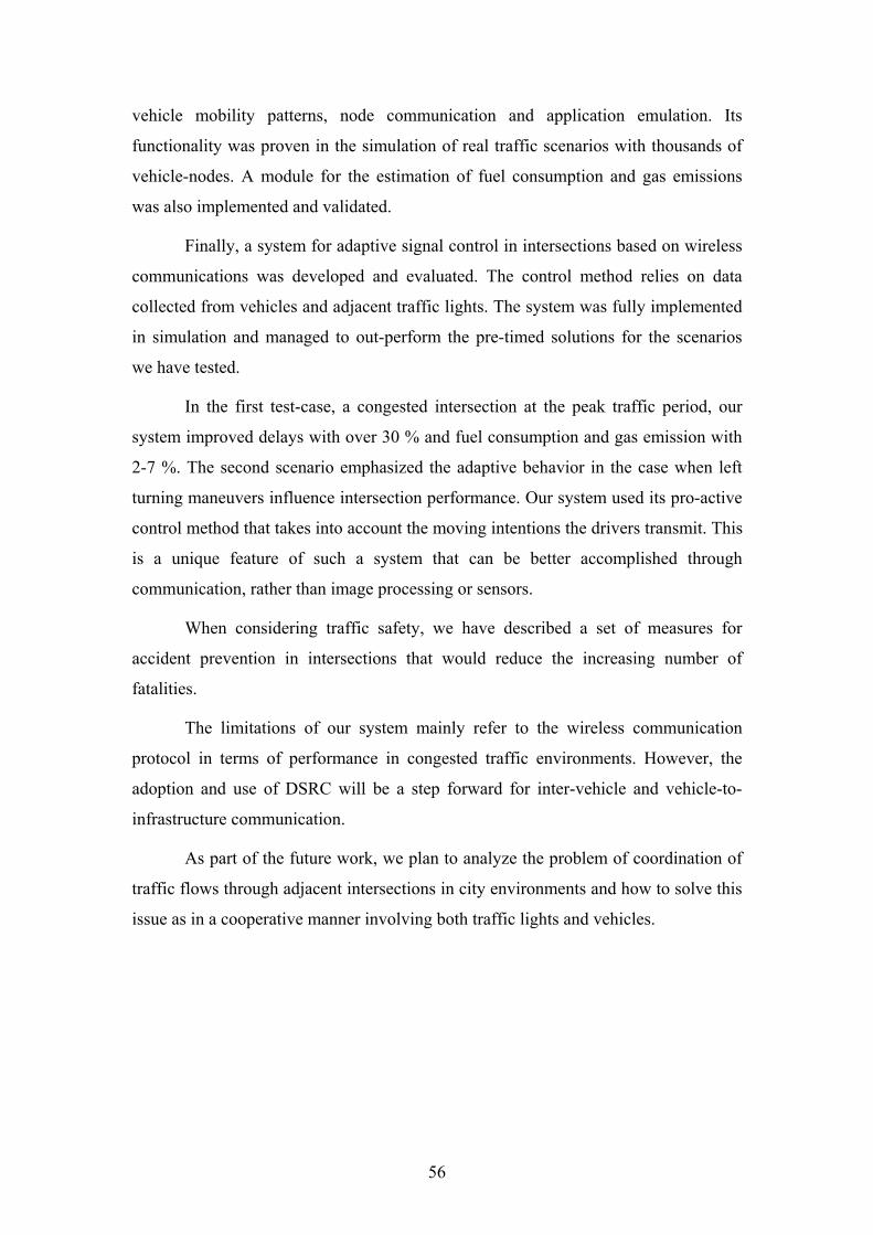
vehicle mobility patterns, node communication and application emulation. Its
functionality was proven in the simulation of real traffic scenarios with thousands of
vehicle-nodes. A module for the estimation of fuel consumption and gas emissions
was also implemented and validated.
Finally, a system for adaptive signal control in intersections based on wireless
communications was developed and evaluated. The control method relies on data
collected from vehicles and adjacent traffic lights. The system was fully implemented
in simulation and managed to out-perform the pre-timed solutions for the scenarios
t can be better accomplished through
The limitations of our system mainly refer to the wireless communication
protocol in terms of performance in congested traffic environments. However, the
for inter-vehicle and vehicle-to-
frastructure communication.
we have tested.
In the first test-case, a congested intersection at the peak traffic period, our
system improved delays with over 30 % and fuel consumption and gas emission with
2-7 %. The second scenario emphasized the adaptive behavior in the case when left
turning maneuvers influence intersection performance. Our system used its pro-active
control method that takes into account the moving intentions the drivers transmit. This
is a unique feature of such a system tha
communication, rather than image processing or sensors.
When considering traffic safety, we have described a set of measures for
accident prevention in intersections that would reduce the increasing number of
fatalities.
adoption and use of DSRC will be a step forward
in
As part of the future work, we plan to analyze the problem of coordination of
traffic flows through adjacent intersections in city environments and how to solve this
issue as in a cooperative manner involving both traffic lights and vehicles.
56
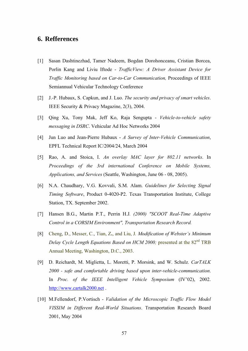
6. Refferences
[1] Sasan Dashtinezhad, Tamer Nadeem, Bogdan Dorohonceanu, Cristian Borcea,
P
ity & Privacy Magazine, 2(3), 2004.
[3] Q
nce on Mobile Systems,
Applications, and Services
ng Software, Product 0-4020-P2. Texas Transportation Institute, College
Station, TX. Septem
an, Z., and Liu, J. Modification of Webster’s Minimum
D
2000 - safe and comfortable driving based upon inter-vehicle-communication.
In Proc. of the IEEE Intelligent Vehicle Symposium (IV’02), 2002.
http://www.cartalk2000.net
orlin Kang and Liviu Iftode - TrafficView: A Driver Assistant Device for
Traffic Monitoring based on Car-to-Car Communication, Proceedings of IEEE
Semiannual Vehicular Technology Conference
[2] J.-P. Hubaux, S. Capkun, and J. Luo. The security and privacy of smart vehicles.
IEEE Secur
ing Xu, Tony Mak, Jeff Ko, Raja Sengupta - Vehicle-to-vehicle safety
messaging in DSRC. Vehicular Ad Hoc Networks 2004
[4] Jun Luo and Jean-Pierre Hubaux - A Survey of Inter-Vehicle Communication,
EPFL Technical Report IC/2004/24, March 2004
[5] Rao, A. and Stoica, I. An overlay MAC layer for 802.11 networks. In
Proceedings of the 3rd international Confere
(Seattle, Washington, June 06 - 08, 2005).
[6] N.A. Chaudhary, V.G. Kovvali, S.M. Alam. Guidelines for Selecting Signal
Timi
ber 2002.
[7] Hansen B.G., Martin P.T., Perrin H.J. (2000) "SCOOT Real-Time Adaptive
Control in a CORSIM Environment", Transportation Research Record.
[8] Cheng, D., Messer, C., Ti
elay Cycle Length Equations Based on HCM 2000; presented at the 82nd TRB
Annual Meeting, Washington, D.C., 2003.
[9] D. Reichardt, M. Miglietta, L. Moretti, P. Morsink, and W. Schulz. CarTALK
.
[10] M.Fellendorf, P.Vortisch - Validation of the Microscopic Traffic Flow Model
VISSIM in Different Real-World Situations. Transportation Research Board
2001, May 2004
57
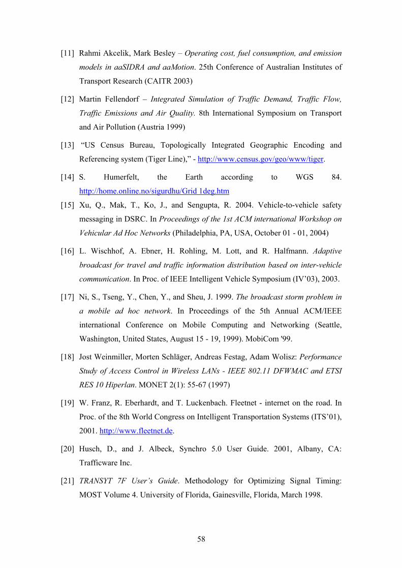
[11] Rahmi Akcelik, Mark Besley – Operating cost, fuel consumption, and emission
RA and aaMotion. 25th Conference of Australian Institutes of
Transport Research (CAITR 2003)
[13] ted Geographic Encoding and
models in aaSID
[12] Martin Fellendorf – Integrated Simulation of Traffic Demand, Traffic Flow,
Traffic Emissions and Air Quality. 8th International Symposium on Transport
and Air Pollution (Austria 1999)
“US Census Bureau, Topologically Integra
Referencing system (Tiger Line),” - http://www.census.gov/geo/www/tiger.
S. Humerfelt, the Earth accor[14] ding to WGS 84.
http://home.online.no/sigurdhu/Grid 1deg.htm
Xu, Q., Mak, T., Ko, J., and Sengupta, R. 2004. V[15] ehicle-to-vehicle safety
A, October 01 - 01, 2004)
3), 2003.
Mobile Computing and Networking (Seattle,
Washington, United States, August 15 - 19, 1999). MobiCom '99.
[18] rmance
Study of Access Control in Wireless LANs - IEEE 802.11 DFWMAC and ETSI
[19] . Fleetnet - internet on the road. In
Proc. of the 8th World Congress on Intelligent Transportation Systems (ITS’01),
messaging in DSRC. In Proceedings of the 1st ACM international Workshop on
Vehicular Ad Hoc Networks (Philadelphia, PA, US
[16] L. Wischhof, A. Ebner, H. Rohling, M. Lott, and R. Halfmann. Adaptive
broadcast for travel and traffic information distribution based on inter-vehicle
communication. In Proc. of IEEE Intelligent Vehicle Symposium (IV’0
[17] Ni, S., Tseng, Y., Chen, Y., and Sheu, J. 1999. The broadcast storm problem in
a mobile ad hoc network. In Proceedings of the 5th Annual ACM/IEEE
international Conference on
Jost Weinmiller, Morten Schläger, Andreas Festag, Adam Wolisz: Perfo
RES 10 Hiperlan. MONET 2(1): 55-67 (1997)
W. Franz, R. Eberhardt, and T. Luckenbach
2001. http://www.fleetnet.de.
Husch, D., and J. Albeck, Synchro 5.0 User Guide. 2001, Albany, CA:
Trafficware Inc.
[20]
[21] TRANSYT 7F User’s Guide. Methodology for Optimizing Signal Timing:
MOST Volume 4. University of Florida, Gainesville, Florida, March 1998.
58
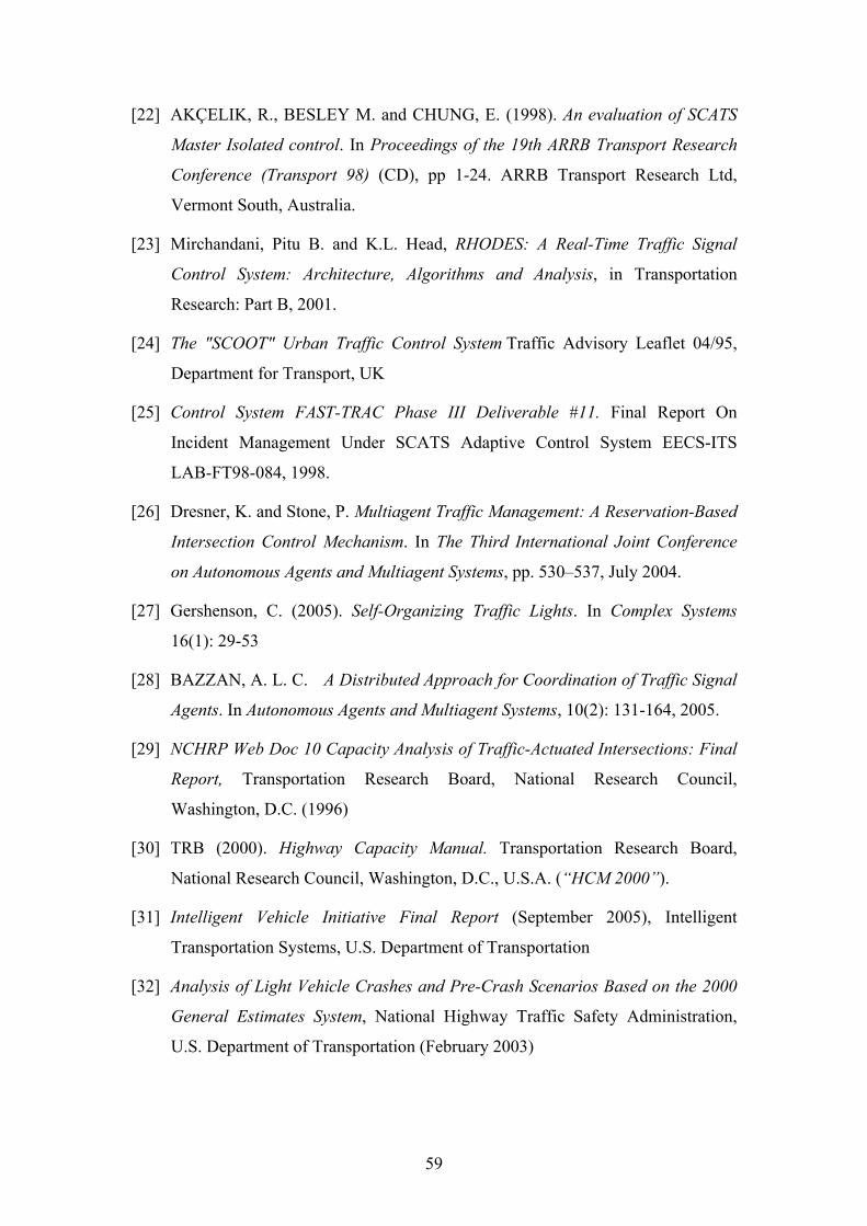
[22] AKÇELIK, R., BESLEY M. and CHUNG, E. (1998). An evaluation of SCATS
Master Isolated control. In Proceedings of the 19th ARRB Transport Research
Conference (Transport 98) (CD), pp 1-24. ARRB Transport Research Ltd,
[23]
Algorithms and Analysis, in Transportation
[24] /95,
[25] verable #11. Final Report On
[26] ed
[27]
[28]
[29] NCHRP Web Doc 10 Capacity Analysis of Traffic-Actuated Intersections: Final
[30] TRB (2000). Highway Capacity Manual. Transportation Research Board,
[31] inal Report (September 2005), Intelligent
Transportation Systems, U.S. Department of Transportation
[32] nd Pre-Crash Scenarios Based on the 2000
General Estimates System, National Highway Traffic Safety Administration,
Vermont South, Australia.
Mirchandani, Pitu B. and K.L. Head, RHODES: A Real-Time Traffic Signal
Control System: Architecture,
Research: Part B, 2001.
The "SCOOT" Urban Traffic Control System Traffic Advisory Leaflet 04
Department for Transport, UK
Control System FAST-TRAC Phase III Deli
Incident Management Under SCATS Adaptive Control System EECS-ITS
LAB-FT98-084, 1998.
Dresner, K. and Stone, P. Multiagent Traffic Management: A Reservation-Bas
Intersection Control Mechanism. In The Third International Joint Conference
on Autonomous Agents and Multiagent Systems, pp. 530–537, July 2004.
Gershenson, C. (2005). Self-Organizing Traffic Lights. In Complex Systems
16(1): 29-53
BAZZAN, A. L. C. A Distributed Approach for Coordination of Traffic Signal
Agents. In Autonomous Agents and Multiagent Systems, 10(2): 131-164, 2005.
Report, Transportation Research Board, National Research Council,
Washington, D.C. (1996)
National Research Council, Washington, D.C., U.S.A. (“HCM 2000”).
Intelligent Vehicle Initiative F
Analysis of Light Vehicle Crashes a
U.S. Department of Transportation (February 2003)
59
[33] Peter M. Knoll, Gerd Teepe; “Das sensitive Auto, mit Sensorik zum
unfallvermeidenden Auto”; auto & elektronik; 2-3/2003
DSRC Home Page - [34] http://www.leearmstrong.com/dsrc/dsrchomeset.htm
[35] http://world.honda.com/news/2005/c050902.html.
C
(W States, December 1998)
[36] Stallard, C. and Owen, L. E. 1998. Evaluating adaptive signal control using
ORSIM. In Proceedings of the 30th Conference on Winter Simulation
ashington, D.C., United
[37] www.daimlerchrysler.com
[38] VISSIM webpage - http://www.english.ptv.de/cgi-bin/traffic/traf_vissim.pl
60