1

Adaptive Transmission Scheduling in Wireless

Networks for Asynchronous Federated

Learning

Hyun-Suk Lee and Jang-Won Lee, Senior Member, IEEE

Abstract

In this paper, we study asynchronous federated learning (FL) in a wireless distributed learning

network (WDLN). To allow each edge device to use its local data more efficiently via asynchronous FL,

transmission scheduling in the WDLN for asynchronous FL should be carefully determined considering

system uncertainties, such as time-varying channel and stochastic data arrivals, and the scarce radio

resources in the WDLN. To address this, we propose a metric, called an effectivity score, which represents

the amount of learning from asynchronous FL. We then formulate an Asynchronous Learning-aware

transmission Scheduling (ALS) problem to maximize the effectivity score and develop three ALS

algorithms, called ALSA-PI, BALSA, and BALSA-PO, to solve it. If the statistical information about

the uncertainties is known, the problem can be optimally and efficiently solved by ALSA-PI. Even if not,

it can be still optimally solved by BALSA that learns the uncertainties based on a Bayesian approach

using the state information reported from devices. BALSA-PO suboptimally solves the problem, but it

addresses a more restrictive WDLN in practice, where the AP can observe a limited state information

compared with the information used in BALSA. We show via simulations that the models trained by

our ALS algorithms achieve performances close to that by an ideal benchmark and outperform those by

other state-of-the-art baseline scheduling algorithms in terms of model accuracy, training loss, learning

speed, and robustness of learning. These results demonstrate that the adaptive scheduling strategy in our

ALS algorithms is effective to asynchronous FL.

Index Terms

Asynchronous learning, distributed learning, federated learning, scheduling, wireless network

H.-S. Lee is with the School of Intelligent Mechatronics Engineering, Sejong University, Seoul 05006, South Korea (e-mail:

hyunsuk@sejong.ac.kr) and J.-W. Lee is with the Department of Electrical and Electronic Engineering, Yonsei University, Seoul

03722, South Korea (e-mail: jangwon@yonsei.ac.kr).

arX

iv:2

103.

0142

2v1

[cs

.IT

] 2

Mar

202

1

2

I. INTRODUCTION

Nowadays, a massive amount of data is generated from edge devices, such as mobile phones

and wearable devices, which can be used for a wide range of machine learning (ML) applications

from healthcare to autonomous driving. As the computational and storage capabilities of such

distributed edge devices keep growing, distributed learning has become attractive to efficiently

exploit the data from edge devices and to address privacy concerns. Due to the emergence of the

need for distributed learning, federated learning (FL) has been widely studied as a potentially

viable solution for distributed learning [1], [2]. FL allows to learn a shared central model from

the locally trained models of distributed edge devices under the coordination of a central server

while the local training data at the edge devices is not shared with the central server.

In FL, the central server and the edge devices should communicate with each other to transmit

the trained models. For this, a wireless network composed of one AP and multiple edge devices

has been widely considered [3]–[10], and the AP in the network plays the role of the central

server in FL. FL is operated in multiple rounds. In each round, first, the AP broadcasts the

current central model. Each edge device substitutes its local model into the received central one

and trains it using its local training data. Then, the locally trained model of each edge device

is uploaded to the AP and the AP aggregates them to update the central model. This enables

training the central model in a distributed manner while avoiding privacy concerns because it

does not require each edge device to upload its local training data.

FL is typically classified into synchronous FL and asynchronous FL [2]. In synchronous FL,

in each round, devices which will train their local models are selected and they synchronously

upload the local models to the AP for aggregation. Then, the AP aggregates them into the central

model after the local models from all the selected devices are received. On the other hand, in

asynchronous FL, in each round, all devices train the local models but only partial devices upload

the local models. Then, each device whose local model has not been uploaded stores its local

model for future use. Hence, asynchronous FL enables each device to continually train its local

model by using the arriving local data in an online manner, which makes FL more effective

and avoids too much pileup of the local data. However, at the same time, it causes the time

lag between the stored local model and the current central model. Such devices who store the

previous local models are typically called stragglers in the literature, and they may cause an

adverse effect to the convergence of the central model because of the time lag [11].

3

Recently, in the ML literature, several works on asynchronous FL have addressed the harmful

effects from the stragglers which inevitably exist due to network circumstances such as time-

varying channels and scarce radio resources [11]–[14]. They introduced various approaches which

address the stragglers when updating the central model and the local models; balancing between

the previous local model and current one [11], [14], adopting dynamic learning rates [11]–[13],

and using a regularized loss function [11], [14]. However, they mainly focused on addressing

the incurred stragglers and did not take into account the issues relevant to the implementation

of FL, which are related to the occurrence of the stragglers. Hence, it is necessary to study an

asynchronous FL procedure in which the key challenges of implementing asynchronous FL in a

wireless network are carefully considered.

When implementing FL in the wireless network, the scarcity of radio resources is one of the

key challenges. Hence, several existing works focus on reducing the communication costs of a

single local model transmission of each edge device; analog model aggregation methods using

the inherent characteristic of a wireless medium [3], [4], a gradient reusing method [15], and

local gradient compressing methods [16], [17]. Meanwhile, other existing works in [5]–[10] focus

on scheduling the transmission of the local models for FL in which only scheduled edge devices

participate in FL. For effective learning, various scheduling strategies for FL have been proposed

based on traditional scheduling policies [5], scheduling criteria to minimize the training loss

[6]–[9], and an effective temporal scheduling pattern to FL [10]. They allow the AP to efficiently

use the radio resources to accelerate FL.

However, these existing works on FL implementation in the wireless network have been studied

only for synchronous FL, and do not consider the characteristics of asynchronous FL, such as

the stragglers and the continual online training of the local models, at all. Nevertheless, the

existing methods on reducing the communication costs can be used for asynchronous FL since in

asynchronous FL, the edge devices should transmit their local model to the AP as in synchronous

FL. On the other hand, the methods on scheduling the transmission of the local models may cause

a significant inefficiency of learning if they are adopted to asynchronous FL. This is because

most of them consider each individual FL round separately and do not address transmission

scheduling over multiple rounds. In asynchronous FL, each round is highly inter-dependent

since the current scheduling affects the subsequent rounds due to the use of the stored local

models from the stragglers. Hence, the transmission scheduling for asynchronous FL should

be carefully determined considering the stragglers over multiple rounds. In addition, in such

4

TABLE ICOMPARISON OF OUR WORK AND RELATED WORKS ON TRANSMISSION SCHEDULING FOR FL (

√: CONSIDERED / ×: NOT

CONSIDERED)

Wireless channel Multiple rounds Stochastic data arrivals Stragglers from async. FL

[5]–[9]√ × × ×

[10]√ √ × ×

Our work√ √ √ √

scheduling over multiple rounds, the effectiveness of learning depends on system uncertainties,

such as time-varying channels and stochastic data arrivals. In particular, the stochastic data

arrivals become more important in asynchronous FL since the data arrivals are directly related to

the amount of the straggled local data due to the continual online training. However, the existing

works do not consider stochastic data arrivals at edge devices.

In this paper, we study asynchronous FL considering the key challenges of implementing it in

a wireless network. To the best of our knowledge, our work is the first to study asynchronous

FL in a wireless network. Specifically, we propose an asynchronous FL procedure in which the

characteristics of asynchronous FL, time-varying channels, and stochastic data arrivals of the

edge devices are considered for transmission scheduling over multiple rounds. The comparison

of our work and the existing works on transmission scheduling in FL is summarized in Table

I. We then analyze the convergence of the asynchronous FL procedure. To address scheduling

the transmission of the local models in the asynchronous FL procedure, we also propose a

metric called an effectivity score. It represents the amount of learning from asynchronous FL

considering the properties of asynchronous FL including the harmful effects on learning due

to the stragglers. We formulate an asynchronous learning-aware transmission scheduling (ALS)

problem to maximize the effectivity score while considering the system uncertainties (i.e., the

time-varying channels and stochastic data arrivals). We then develop the following three ALS

algorithms that solve the ALS problem:

• First, an ALS algorithm with the perfect statistical information about the system uncertainties

(ALSA-PI) optimally and efficiently solves the problem using the state information reported

from the edge devices in the asynchronous FL procedure and the statistical information.

• Second, a Bayesian ALS algorithm (BALSA) solves the problem using the state information

without requiring any a priori information. Instead, it learns the system uncertainties based

on a Bayesian approach. We prove that BALSA is optimal in terms of the long-term average

effectivity score by its regret bound analysis.

5

TABLE IILIST OF NOTATIONS

Notation Description Notation Descriptionw𝑡 Central parameters of the AP in round 𝑡 ℎ𝑡𝑢 Channel gain of device 𝑢 in round 𝑡

w𝑡𝑢 Local parameters of device 𝑢 in round 𝑡 𝑎𝑡𝑢 Transmission scheduling indicator of device 𝑢 in round 𝑡

𝑐𝑡𝑢 Central learning weight of device 𝑢 in round 𝑡 𝑥𝑡𝑢 Successful transmission indicator of device 𝑢 in round 𝑡

𝑛𝑡𝑢 Number of aggregated samples of device 𝑢 up to round 𝑡 − 1after the latest successful local update transmission

𝛉𝐶𝑢 Parameters of the channel gain of device 𝑢

𝑚𝑡𝑢 Number of arrived samples of device 𝑢 during round 𝑡 \𝑃

𝑢 Parameter of the sample arrival of device 𝑢

𝑁 𝑡𝑢 Total number of samples from device 𝑢 used for the central

updates up to round 𝑡 − 1`1 Prior distribution for the parameters 𝛉

Δ𝑡𝑢 Local update of device 𝑢 in round 𝑡 `𝑡 Posterior distribution for the parameters 𝛉 in round 𝑡

[𝑡𝑢 Local learning rate of device 𝑢 in round 𝑡 𝑡𝑘 Start time of stage 𝑘 of BALSA

𝜓𝑡𝑢 Local gradient of device 𝑢 in round 𝑡 𝑇𝑘 Length of stage 𝑘 of BALSA

• Third, a Bayesian ALS algorithm for a partially observable WDLN (BALSA-PO) solves the

problem only using partial state information (i.e., channel conditions). It addresses a more

restrictive WDLN in practice, where each edge device is allowed to report only its current

channel condition to the AP.

Through experimental results, we show that ALSA-PI and BALSAs (i.e., BALSA and BALSA-

PO) achieve performance close to an ideal benchmark with no radio resource constraints and

transmission failure. We also show that they outperform other baseline scheduling algorithms

in terms of training loss, test accuracy, learning speed, and robustness of learning.

The rest of this paper is organized as follows. Section II introduces a WDLN with asynchronous

FL. In Section III, we formulate the ALS problem considering asynchronous FL. In Section IV,

we develop ALSA-PI, BALSA, and BALSA-PO, and in Section V, we provide experimental

results. Finally, we conclude in Section VI.

II. WIRELESS DISTRIBUTED LEARNING NETWORK WITH ASYNCHRONOUS FL

In this section, we introduce typical learning strategies of asynchronous FL provided in [11]–

[14]. We then propose an asynchronous FL procedure to adopt the learning strategies in a WDLN.

For ease of reference, we summarize some notations in Table II.

A. Central and Local Parameter Updates in Asynchronous FL

Here, we introduce typical learning strategies to update the central and local parameters in

asynchronous FL [11]–[14], which address the challenges due to the stragglers. To this end,

we consider one access point (AP) that plays a role of a central server in FL and 𝑈 edge

devices. The set of edge devices is defined as U = {1, 2, ...,𝑈}. In asynchronous FL, an artificial

6

neural network (ANN) model composed of multiple parameters is trained in a distributed manner

to minimize an empirical loss function 𝑙 (w), where w denotes the parameters of the ANN.

Asynchronous FL proceeds over a discrete-time horizon composed of multiple rounds. The set of

rounds is defined as T = {1, 2, ...} and the index of rounds is denoted by 𝑡. Then, we can formally

define the problem of asynchronous FL with a given local loss function at device 𝑢, 𝑓𝑢, as follows:

minimizew

𝑙 (w) = 1𝐾

𝑈∑𝑢=1

𝐾𝑢∑𝑘=1

𝑓𝑢 (w, 𝑘), (1)

where 𝐾𝑢 denotes the number of data samples of device 𝑢,1 𝐾 =∑𝑈𝑢=1 𝐾𝑢, and 𝑓𝑢 (w, 𝑘) is an

empirical local loss function defined by the parameters w at 𝑘-th data sample of device 𝑢. To solve

this problem, in asynchronous FL, each device trains parameters by using its locally available

data and transmits the trained parameters to the AP. Then, the AP updates its parameters by

using the parameters from each device. We call the parameters at the AP central parameters

and those at each device local parameters. The details of how to update the central and local

parameters in asynchronous FL are provided in the following.

1) Central Parameter Updates: Let the central parameters of the AP and the local parameters

of device 𝑢 in round 𝑡 be denoted by w𝑡 and w𝑡𝑢, respectively. After the scheduled devices transmit

their local parameters to the AP, the AP updates its central parameters by aggregating the received

local parameters. Let U𝑡 be the set of the devices whose local parameters are successfully received

at the AP in round 𝑡. Then, the AP can updates its central parameter as follows [11], [13]:

w𝑡+1 = w𝑡 −∑𝑢∈U𝑡

𝑐𝑡𝑢 (w𝑡𝑢 − w𝑡+1

𝑢 )

= w𝑡 −∑𝑢∈U𝑡

𝑐𝑡𝑢 (w𝑡𝑢 − (w𝑡

𝑢 − Δ𝑡𝑢))

= w𝑡 −∑𝑢∈U𝑡

𝑐𝑡𝑢Δ𝑡𝑢, (2)

where 𝑐𝑡𝑢 is the central learning weight of device 𝑢 in round 𝑡 and Δ𝑡𝑢 B w𝑡+1𝑢 − w𝑡

𝑢 is the local

update on the local data samples of device 𝑢 in round 𝑡. We define the total number of samples

from device 𝑢 used for the central updates up to round 𝑡 − 1 as 𝑁 𝑡𝑢, the number of aggregated

samples of device 𝑢 up to round 𝑡 − 1 after the latest successful local update transmission as

𝑛𝑡𝑢, and the number of samples of device 𝑢 that have arrived during round 𝑡 as 𝑚𝑡𝑢. Then, the

1For simple presentation, we omit the word “edge” from edge device in the rest of the paper.

7

central learning weight of device 𝑢 in round 𝑡 is determined according to the numbers of the

samples used for the central parameter updates from the devices so far:

𝑐𝑡𝑢 =𝑁 𝑡𝑢 + 𝑛𝑡𝑢 + 𝑚𝑡𝑢∑

𝑢∈U 𝑁𝑡𝑢 +

∑𝑢∈U𝑡 𝑛𝑡𝑢 + 𝑚𝑡𝑢

.

2) Local Parameter Updates: We describe local parameter updates at each device in asyn-

chronous FL. In round 𝑡, the AP broadcasts the central parameters w𝑡 to all devices and each device

𝑢 updates its local parameters w𝑡𝑢 to be w𝑡 . Then, the device trains its local parameters using its local

data samples that have arrived since its previous local parameter update, 𝑚𝑡𝑢. To this end, it applies

a gradient-based update method using the regularized loss function defined as follows [11], [14]:

𝑠𝑢 (w𝑡𝑢) = 𝑓𝑢 (w𝑡

𝑢) +_

2| |w𝑡

𝑢 − w𝑡 | |,

where the second term mitigates the deviations of the local parameters from the central ones

and _ is the parameter for the regularization. We denote the local gradient of device 𝑢 calculated

using its local data samples in round 𝑡 by ∇𝑔𝑡𝑢. In asynchronous FL, the local gradient which

has not been transmitted in the previous rounds will be aggregated to the current local gradient.

Such local gradients not transmitted in the previous rounds are called delayed local gradients.

In the literature, the devices who have such delayed local gradients are called stragglers. It has

been shown that they adversely affect model convergence since the parameters used to calculate

the delayed local gradients are different from the current local parameters used to calculate the

current local gradients [11], [14], [18].

To address this issue, when aggregating the previous local gradients and current ones, we need

to balance between them. To this end, in [11], [14], the decay coefficient 𝛽 is introduced and

used when aggregating the local gradients as

𝜓𝑡𝑢 = ∇𝑔𝑡𝑢 + 𝛽𝜓𝑡−1𝑢 , (3)

where 𝜓𝑡𝑢 is the aggregated local gradient of device 𝑢 in round 𝑡. By using the aggregated local

gradient, we define the local update of device 𝑢 in round 𝑡 as

Δ𝑡𝑢 = [𝑡𝑢𝜓

𝑡𝑢, (4)

where [𝑡𝑢 is the local learning rate of the local parameters of device 𝑢 in round 𝑡. Moreover,

a dynamic local learning rate has been widely applied to address the stragglers. The dynamic

8

learning rate of device 𝑢 in round 𝑡 is determined as follows [11], [13], [19]:

[𝑡𝑢 = [𝑑 max{1, log

(𝑑𝑡𝑢)}, (5)

where [𝑑 is an initial value of the local learning rate and 𝑑𝑡𝑢 is a delay cost depending on the

rounds since the latest successful local update transmission of device 𝑢 in round 𝑡. Note that the

delay cost can be chosen according to the characteristics of the system. Each device transmits

its local update Δ𝑡𝑢 to the AP according to the transmission scheduling, and then, updates its

aggregated local gradient according to the local update transmission as

𝜓𝑡𝑢 =

0, if device 𝑢 successfully transmit its local update

𝜓𝑡𝑢, otherwise.(6)

B. Asynchronous FL Procedure in WDLN

We consider a WDLN consisting of one AP and 𝑈 devices that cooperatively operate FL over

the discrete-time horizon composed of multiple rounds. In the WDLN, the local data stochastically

and continually arrives at each device and the device trains its local parameters in each round

by using the arrived data. Due to the scarce radio resources of the WDLN, it is impractical that

all devices transmit their local parameters to the AP simultaneously. Hence, FL in the WDLN

becomes asynchronous FL and the devices who will transmit their local parameters in each round

should be carefully scheduled by the AP for training the central parameters effectively.

We now propose an asynchronous FL procedure for the WDLN in which the central and local

parameter update strategies introduced in the previous subsection are adopted. In the procedure,

the characteristics of the WDLN, such as time-varying channel conditions and system bandwidth,

are considered as well. This allows us to implement asynchronous FL in the WDLN while

addressing the challenges due to the scarcity of radio resources in the WDLN. We denote the

channel gain of device 𝑢 in round 𝑡 by ℎ𝑡𝑢. We assume that the channel gain of device 𝑢 in each

round follows a parameterized distribution and denote the corresponding parameters by 𝛉𝐶𝑢 . The

vector of the channel gain in round 𝑡 is defined by h𝑡 = {ℎ𝑡𝑢}𝑢∈U .

Each round 𝑡 in the procedure composed of three phases: transmission scheduling phase,

local parameter update phase, and parameter aggregation phase. In the transmission scheduling

phase, the AP observes the state information of the devices which can be used to determine the

transmission scheduling. In specific, we define the state information in round 𝑡 as s𝑡 = (h𝑡 , n𝑡),

9

Round t

Report state information and (only in partially observable WDLN)

Transmit local update and

AP

Device u

Round t+1Round t-1

Updateand

Aggregate receivedlocal updates for

Substitute local parameters& Compute local update

Broadcast central parameters& scheduling indicator

Transmission scheduling phase

Local parameter update phase

Parameter aggregation phaseTime

Schedule devices

Fig. 1. The asynchronous FL procedure in the WDLN.

where n𝑡 = {𝑛𝑡𝑢}𝑢∈U is the vector of the number of aggregated samples of each device up to round

𝑡 − 1 after its latest successful local update transmission. It is worth noting that in the following

sections, we consider a partially observable WDLN as well, in which the AP can observe the

channel gain h𝑡 only, to address more restrictive environments in practice. Then, the AP determines

the transmission scheduling for asynchronous FL based on the state information. In the local

parameter update phase, the AP broadcasts its central parameters w𝑡 to all devices. We assume that

all devices receive w𝑡 successfully because the AP can reliably broadcast the central parameters by

using much larger power than the devices and robust transmission methods considering the worst-

case device.2 Each device 𝑢 replaces its local parameters with the received central parameters.

Then, it trains the parameters using its local data samples which have arrived since the local

parameter update phase in the previous round and calculates the local update Δ𝑡𝑢 in (4) as described

in Section II-A2. Finally, in the parameter aggregation phase, each scheduled device transmits

its local update to the AP. Then, the AP updates the central parameters by averaging them as in

(2). In the following, we describe the asynchronous FL procedure in the WDLN in more detail.

First, the AP schedules the devices to transmit their local updates based on the state information

to effectively utilize the limited radio resources in each round. We define the maximum number

of devices that can be scheduled in each round as 𝑊 . It is worth noting that 𝑊 is restricted by the

bandwidth of the WDLN and typically much smaller than the number of devices 𝑈 (i.e., 𝑊 � 𝑈).

We define a transmission scheduling indicator of device 𝑢 in round 𝑡 as 𝑎𝑡𝑢 ∈ {0, 1}, where 1

represents device 𝑢 is scheduled to transmit its gradient in round 𝑡 and 0 represents it is not. The

vector of the transmission scheduling indicators in round 𝑡 is defined as a𝑡 = {𝑎𝑡𝑢}𝑢∈U . In round

2It is worth noting that this assumption is only to avoid unnecessarily complicated modeling. We can easily extend ourproposed method for the model without this assumption by allowing each device to maintain its previous local parameters whenits reception of the central parameters is failed.

10

𝑡, the AP schedules the devices to transmit their local updates satisfying the following constraint:∑𝑢∈U

𝑎𝑡 = 𝑊.

Then, according to the channel gains, the probability of successful transmission is determined. We

define the successful transmission indicator of the local update of device 𝑢 in round 𝑡 as a Bernoulli

random variable 𝑥𝑡𝑢, where 1 represents the successful transmission and 0 represents the transmis-

sion failure. To model the indicator as a Bernoulli random variable, we can use the approximation

of the packet error rate (PER) with the given signal-to-interference-noise ratio (SINR) [20], [21].

For example, the PER of an uncoded packet can be given by P[𝑥 = 0|Φ] = 1−(1−𝑏(Φ))𝑛, where Φ

is the SINR with the channel gain ℎ, 𝑏(·) is the bit error rate for the given SINR, and 𝑛 is the packet

length in bits. We refer the readers to [21] for more examples of the PER approximations with

coding. The vector of the successful transmission indicators in round 𝑡 is defined as x𝑡 = {𝑥𝑡𝑢}𝑢∈U .

We assume the number of the samples that have arrived at device 𝑢 during round 𝑡, 𝑚𝑡𝑢, is an

independently and identically distributed (i.i.d.) Poisson random variable with a parameter \𝑢.3

At the end of round 𝑡, the number of aggregated samples of device 𝑢 up to round 𝑡 after the

latest successful local update transmission,4 𝑛𝑡+1𝑢 , and the total number of samples from device 𝑢

used for the central updates up to round 𝑡, 𝑁 𝑡+1𝑢 , should be calculated depending on the local

update transmission as follows:

𝑛𝑡+1𝑢 =

0, 𝑎𝑡𝑢 = 1 and 𝑥𝑡𝑢 = 1

𝑛𝑡𝑢 + 𝑚𝑡𝑢, otherwise(7)

and

𝑁 𝑡+1𝑢 =

𝑁 𝑡𝑢 + 𝑛𝑡𝑢 + 𝑚𝑡𝑢, 𝑎𝑡𝑢 = 1 and 𝑥𝑡𝑢 = 1

𝑁 𝑡𝑢, otherwise.(8)

With the scheduling and successful transmission indicators, we can rewrite the equation for the

3It is worth noting that the assumption of Poisson data arrivals is only for simple implementation of the Bayesian approachin our proposed method. We can easily generalize our proposed method for any other i.i.d. data arrivals by using samplingalgorithms such as Gibbs sampling.

4For brevity, we simply write “the number of aggregated samples of device 𝑢 in round 𝑡” to denote 𝑛𝑡𝑢 in the rest of this paper.

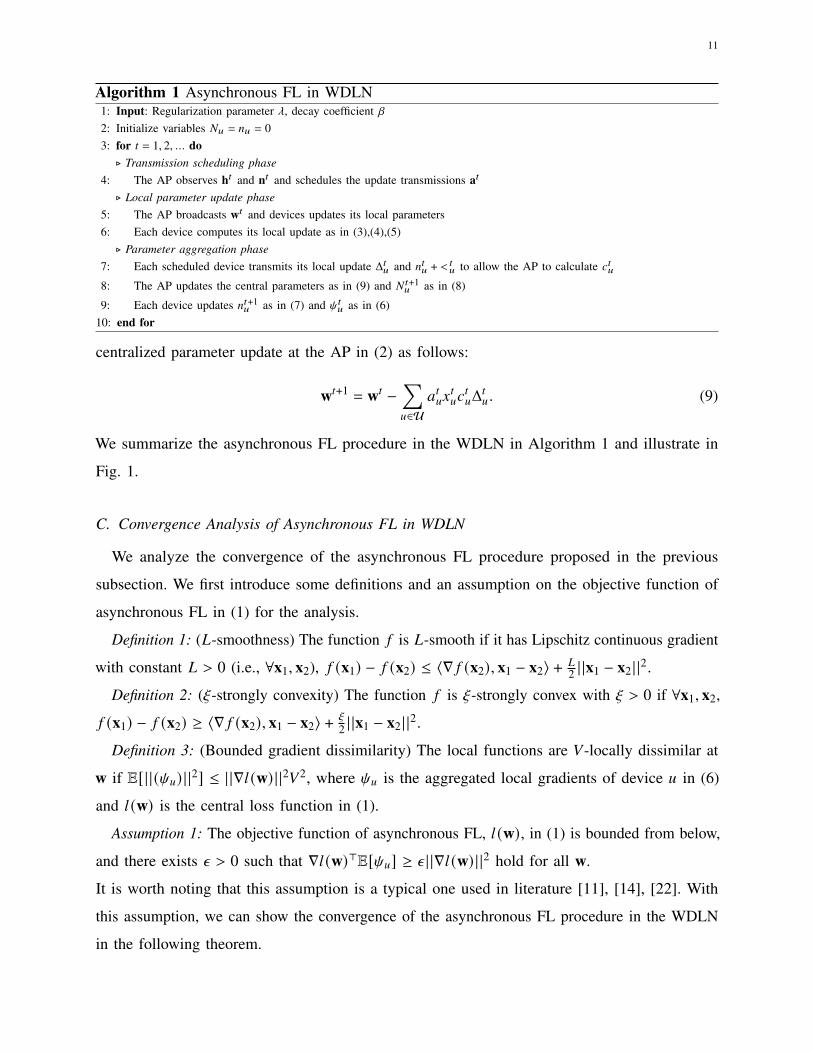
11

Algorithm 1 Asynchronous FL in WDLN1: Input: Regularization parameter _, decay coefficient 𝛽2: Initialize variables 𝑁𝑢 = 𝑛𝑢 = 03: for 𝑡 = 1, 2, ... do⊲ Transmission scheduling phase

4: The AP observes h𝑡 and n𝑡 and schedules the update transmissions a𝑡

⊲ Local parameter update phase5: The AP broadcasts w𝑡 and devices updates its local parameters6: Each device computes its local update as in (3),(4),(5)⊲ Parameter aggregation phase

7: Each scheduled device transmits its local update Δ𝑡𝑢 and 𝑛𝑡𝑢 + 𝑚𝑡

𝑢 to allow the AP to calculate 𝑐𝑡𝑢8: The AP updates the central parameters as in (9) and 𝑁 𝑡+1

𝑢 as in (8)

9: Each device updates 𝑛𝑡+1𝑢 as in (7) and 𝜓𝑡𝑢 as in (6)10: end for

centralized parameter update at the AP in (2) as follows:

w𝑡+1 = w𝑡 −∑𝑢∈U

𝑎𝑡𝑢𝑥𝑡𝑢𝑐𝑡𝑢Δ

𝑡𝑢 . (9)

We summarize the asynchronous FL procedure in the WDLN in Algorithm 1 and illustrate in

Fig. 1.

C. Convergence Analysis of Asynchronous FL in WDLN

We analyze the convergence of the asynchronous FL procedure proposed in the previous

subsection. We first introduce some definitions and an assumption on the objective function of

asynchronous FL in (1) for the analysis.

Definition 1: (𝐿-smoothness) The function 𝑓 is 𝐿-smooth if it has Lipschitz continuous gradient

with constant 𝐿 > 0 (i.e., ∀x1, x2), 𝑓 (x1) − 𝑓 (x2) ≤ 〈∇ 𝑓 (x2), x1 − x2〉 + 𝐿2 | |x1 − x2 | |2.

Definition 2: (b-strongly convexity) The function 𝑓 is b-strongly convex with b > 0 if ∀x1, x2,

𝑓 (x1) − 𝑓 (x2) ≥ 〈∇ 𝑓 (x2), x1 − x2〉 + b

2 | |x1 − x2 | |2.Definition 3: (Bounded gradient dissimilarity) The local functions are 𝑉-locally dissimilar at

w if E[| | (𝜓𝑢) | |2] ≤ ||∇𝑙 (w) | |2𝑉2, where 𝜓𝑢 is the aggregated local gradients of device 𝑢 in (6)

and 𝑙 (w) is the central loss function in (1).

Assumption 1: The objective function of asynchronous FL, 𝑙 (w), in (1) is bounded from below,

and there exists 𝜖 > 0 such that ∇𝑙 (w)>E[𝜓𝑢] ≥ 𝜖 | |∇𝑙 (w) | |2 hold for all w.

It is worth noting that this assumption is a typical one used in literature [11], [14], [22]. With

this assumption, we can show the convergence of the asynchronous FL procedure in the WDLN

in the following theorem.

12

Theorem 1: Suppose that the objective function of asynchronous FL in the WDLN, 𝑙 (w), in

(1) is 𝐿-smooth and b-strongly convex, and the local gradients 𝜓𝑢’s are 𝑉-dissimilar. Then, if

Assumption 1 holds and [ ≤ [𝑡𝑢 < [𝑡 = 2𝜖𝐿𝑈𝑉2 (max𝑢∈U{𝑐𝑡𝑢})−1, after 𝑇 rounds, the asynchronous

FL procedure in the WDLN satisfies

E[𝑙 (w𝑇 ) − 𝑙 (w∗)] ≤ (1 − 2b[𝑈𝜖′)𝑇 (𝑙 (w0) − 𝑙 (w∗)),

where 𝜖′ = 𝜖 − 𝐿[𝑡𝑉2

2 .

Proof: See Appendix A.

Theorem 1 theoretically shows the convergence of the asynchronous FL procedure in the WDLN

as 𝑇 →∞ since 0 < 2b[𝑈𝜖′ < 1. However, various aspects in learning, such as a learning speed

and a robustness to stragglers, are not directly shown in this theorem, and they may appear

differently according to transmission scheduling strategies used in the asynchronous FL procedure

as will be shown in Section V.

III. PROBLEM FORMULATION

We now formulate an asynchronous learning-aware transmission scheduling (ALS) problem to

maximize the performance of FL learning. In the literature, it is empirically shown that the FL

learning performance mainly depends on the local update of each device, which is determined

by the arrived data samples at the devices [2], [14]. However, it is still not clearly investigated

which characteristics in a local update bring a larger impact than others to learn the optimal

parameters [2], [23]. Moreover, it is hard for the AP to exploit information relevant to the local

updates because the AP cannot obtain the local updates before the devices transmit them to the

AP and cannot access the data samples of the devices due to the limited radio resources and

privacy issues. Due to these reasons, instead of directly finding the impactful local updates, the

existing works [7]–[9] schedule the transmissions according to the factors in the bound of the

convergence rate of FL, which implicitly represent the impact of the local updates in terms of the

convergence. However, as pointed out in Section I, the existing works on transmission scheduling

for FL do not consider asynchronous FL over multiple rounds. As a result, their scheduling

criterion based on the convergence rate may become inefficient in asynchronous FL since in a

long-term aspect with asynchronous FL, the deterioration of the central model’s convergence due

to the absence of some devices in model aggregation can be compensated later thanks to the

nature of asynchronous FL.

13

Contrary to the existing works, we focus on maximizing the average number of learning

from the local data samples considering asynchronous FL. The number of data samples used in

learning can implicitly represent the amount of learning. Roughly speaking, a larger number of

data samples leads the empirical loss in (1) to be converged into a true one in the real-world. It

is also empirically accepted in the literature that more amount of data samples generally results

in better performance [24], [25]. In this context, in FL, the number of the local samples used

to calculate the local gradients represents the amount of learning since the central parameters

are updated by aggregating the local gradients. However, in asynchronous FL, the delayed local

gradients due to scheduling or transmission failure are aggregated to the current one, which may

cause an adverse effect on learning. Hence, here, we maximize the total number of samples used

to calculate the local gradients aggregated in the central updates while considering their delay as

a cost to minimize its adverse effect on learning.

We define a state in round 𝑡 by a tuple of the channel gain h𝑡 and the numbers of the

aggregated samples n𝑡 , s𝑡 = (h𝑡 , n𝑡) and the state space S ⊂ R𝑈 × N𝑈 . The AP can observe the

state information in the transmission scheduling phase of each round. It is worth noting that in the

following section, we will also consider the more restrictive environments in which the AP can

observe only a partial state in round 𝑡 (i.e., the channel gain h𝑡). We denote system uncertainties

in the WDLN, such as the successful local update transmissions and data sample arrivals, by

random disturbances. The vector of the random disturbances in round 𝑡 is defined as v𝑡 = (x𝑡 ,m𝑡),where x𝑡 is the vector of the successful transmission indicators in round 𝑡 and m𝑡 is the vector of

the number of samples that have arrived at each device during round 𝑡. Then, an action in round

𝑡, a𝑡 , is chosen from the action space, defined by A = {a :∑𝑢∈U 𝑎𝑢 = 𝑊}. In each round 𝑡, the

AP determines the action based on the observed state while considering the random disturbances

which are unknown to the AP. To evaluate the effectiveness of the transmission on learning in

each round, we define a metric, called an effectivity score of asynchronous FL, as

𝐹 (s𝑡 , a𝑡 , v𝑡) =∑𝑢∈U𝑡

𝑛𝑡𝑢 + 𝑚𝑡𝑢 −∑

𝑢∈U\U𝑡

𝛾(𝑛𝑡𝑢 + 𝑚𝑡𝑢), (10)

where U𝑡 is the set of the devices whose local update transmission was successful in round 𝑡 and

𝛾 ∈ [0, 1) is a delay cost to consider the adverse effect of the stragglers. This effectivity score

represents the total number of the samples that will be effectively used in the central update

considering the delay cost in asynchronous FL. We now formulate the ALS problem maximizing

14

the total expected effectivity score of asynchronous FL as

maximize𝜋

lim𝑇→∞

E

[𝑇∑𝑡=1

𝐹 (s𝑡 , a𝑡 , v𝑡)], (11)

where 𝜋 : S → A is a policy that maps a state to an action. This problem maximizes the number

of samples used in asynchronous FL while trying to minimize the adverse effect of the stragglers

due to the delay.

We define the parameters for the the channel gain and the average number of arrived samples

(i.e., arrival rate) of each device in each round as 𝛉 = {𝛉𝐶1 , ..., 𝛉𝐶𝑈 , \

𝑃1 , ..., \

𝑃𝑈} ∈ Θ, where Θ is

a parameter space. These parameters express the system uncertainties in the WDLN, and thus,

we can solve the problem if they are known. We define the true parameters for the WDLN as

𝛉∗ = {𝛉∗,𝐶 , 𝛉∗,𝑃}, where 𝛉∗,𝐶 and 𝛉∗,𝑃 are the true parameters for the channel gains and the arrival

rates, respectively. Formally, if the parameters 𝛉∗ are perfectly known as a priori information,

the state transition probabilities, P[s′|s, a], can be derived by using the probability of successful

transmission, the distribution of the channel gains, and the Poisson distribution with the a priori

information. Then, based on the transition probabilities, the problem in (11) can be optimally

solved by standard dynamic programming (DP) methods [26]. However, this is impractical since

it is hard to obtain such a priori information in advance. Besides, even if such a priori information

is perfectly known, the computational complexity of the standard DP methods is too high as will

be shown in Section IV-E. Hence, we need a learning approach such as reinforcement learning

(RL) that learns the information while proceeding the asynchronous FL, and develop algorithms

based on it in the following section.

IV. ASYNCHRONOUS LEARNING-AWARE TRANSMISSION SCHEDULING

In this section, we develop three ALS algorithms each of which requires different information

to solve the ALS problem: an ALS algorithm with perfect a priori information (ALSA-PI), a

Bayesian ALS algorithm (BALSA), and a Bayesian ALS algorithm with a partially observable

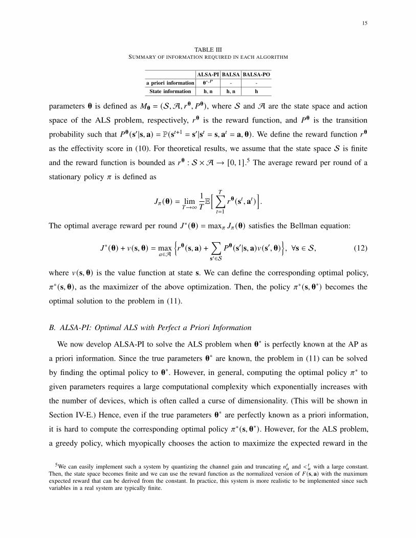
state information (BALSA-PO). We summarize the information required in ASLA-PI, BALSA,

and BALSA-PO in Table III.

A. Parametrized Markov Decision Process

Before developing algorithms, we first define a parameterized Markov decision process (MDP)

based on the ALS problem in the previous section. The MDP parameterized by the unknown

15

TABLE IIISUMMARY OF INFORMATION REQUIRED IN EACH ALGORITHM

ALSA-PI BALSA BALSA-POa priori information 𝛉∗,𝑃 - -

State information h, n h, n h

parameters 𝛉 is defined as 𝑀𝛉 = (S,A, 𝑟𝛉, 𝑃𝛉), where S and A are the state space and action

space of the ALS problem, respectively, 𝑟𝛉 is the reward function, and 𝑃𝛉 is the transition

probability such that 𝑃𝛉(s′|s, a) = P(s𝑡+1 = s′|s𝑡 = s, a𝑡 = a, 𝛉). We define the reward function 𝑟𝛉

as the effectivity score in (10). For theoretical results, we assume that the state space S is finite

and the reward function is bounded as 𝑟𝛉 : S ×A → [0, 1].5 The average reward per round of a

stationary policy 𝜋 is defined as

𝐽𝜋 (𝛉) = lim𝑇→∞

1𝑇E[ 𝑇∑𝑡=1

𝑟𝛉(s𝑡 , a𝑡)].

The optimal average reward per round 𝐽∗(𝛉) = max𝜋 𝐽𝜋 (𝛉) satisfies the Bellman equation:

𝐽∗(𝛉) + 𝑣(s, 𝛉) = max𝑎∈A

{𝑟𝛉(s, a) +

∑s′∈S

𝑃𝛉(s′|s, a)𝑣(s′, 𝛉)}, ∀s ∈ S, (12)

where 𝑣(s, 𝛉) is the value function at state s. We can define the corresponding optimal policy,

𝜋∗(s, 𝛉), as the maximizer of the above optimization. Then, the policy 𝜋∗(s, 𝛉∗) becomes the

optimal solution to the problem in (11).

B. ALSA-PI: Optimal ALS with Perfect a Priori Information

We now develop ALSA-PI to solve the ALS problem when 𝛉∗ is perfectly known at the AP as

a priori information. Since the true parameters 𝛉∗ are known, the problem in (11) can be solved

by finding the optimal policy to 𝛉∗. However, in general, computing the optimal policy 𝜋∗ to

given parameters requires a large computational complexity which exponentially increases with

the number of devices, which is often called a curse of dimensionality. (This will be shown in

Section IV-E.) Hence, even if the true parameters 𝛉∗ are perfectly known as a priori information,

it is hard to compute the corresponding optimal policy 𝜋∗(s, 𝛉∗). However, for the ALS problem,

a greedy policy, which myopically chooses the action to maximize the expected reward in the

5We can easily implement such a system by quantizing the channel gain and truncating 𝑛𝑡𝑢 and 𝑚𝑡𝑢 with a large constant.

Then, the state space becomes finite and we can use the reward function as the normalized version of 𝐹 (s, a) with the maximumexpected reward that can be derived from the constant. In practice, this system is more realistic to be implemented since suchvariables in a real system are typically finite.

16

current round, becomes the optimal policy thanks to the structure of the reward as the following

theorem.

Theorem 2: For the parameterized MDP with given finite parameters, the greedy policy in

(14) is optimal.

Proof: See Appendix B.

With this theorem, we can easily develop ALSA-PI by adopting the greedy policy with the known

parameters 𝛉∗.

In round 𝑡, the greedy policy for given parameters 𝛉 chooses the action by solving the following

optimization problem:

maximizea∈A

E[𝐹 (s𝑡 , a, v𝑡) |𝛉],

where E[·|𝛉] represents the expectation over the probability distribution of the given parameters

𝛉. We rearrange the objective function in (10) as

𝐹 (s𝑡 , a, v𝑡) =∑𝑢∈U

𝑎𝑢𝑥𝑡𝑢 (1 + 𝛾) (𝑛𝑡𝑢 + 𝑚𝑡𝑢) − 𝛾(𝑛𝑡𝑢 + 𝑚𝑡𝑢). (13)

Then, we can reformulate the problem as

maximizea∈A

∑𝑢∈U

𝑎𝑢E[𝑥𝑡𝑢 (𝑛𝑡𝑢 + 𝑚𝑡𝑢) |𝛉𝑃],

since the last term in (13) does not depend on both transmission scheduling indicator a and

uncertainty on the successful transmission x𝑡 . In addition, the conditional expectation in the

problem depends only on the parameters for the arrival rates of the data samples, 𝛉𝑃 = {\𝑃1 , ...\𝑃𝑈},

because 𝑥𝑡𝑢 is solely determined by the current channel gain. Let the devices be sorted in descending

order of their expected number of samples E[𝑥𝑡𝑢 (𝑛𝑡𝑢 + 𝑚𝑡𝑢) |𝛉𝑃] and indexed by (1), (2), ..., (𝑈).Then, the greedy policy in round 𝑡 is easily obtained as

𝜋𝑔 (s𝑡 , 𝛉𝑃) =

𝑎𝑢 = 1, 𝑢 ∈ {(1), ..., (𝑊)}

𝑎𝑢 = 0, otherwise.(14)

In ALSA-PI, the AP schedules the devices according to the greedy policy with the true parameter

𝛉∗,𝑃 (i.e., 𝜋𝑔 in (14) with 𝛉∗,𝑃) in each round.

17

C. BALSA: Optimal Bayesian ALS without a Priori Information

We now develop BALSA that solves the parameterized MDP without requiring any a priori

information. To this end, it adopts a Bayesian approach to learn the unknown parameters 𝛉. We

define the policy determined by BALSA as 𝜙 = (𝜙1, 𝜙2, ...) each of which 𝜙𝑡 (g𝑡) chooses an action

according to the history of states, actions, and rewards, g𝑡 = (s1, ..., s𝑡 , a1, ..., a𝑡−1, 𝑟1, ..., 𝑟 𝑡−1). To

apply the Bayesian approach, we assume that the parameters that belong to 𝛉 are independent to

each other. We denote a prior distribution for the parameters 𝛉 by `1. For the prior distribution, the

non-informative prior can be typically used if there is no prior information about the parameters.

On the other hand, if there is any prior information, then it can be defined by considering the

information. For example, if we know that a parameter belongs to a certain interval, then the

prior distribution can be defined as a truncated distribution whose probability measure outside of

the interval is zero. We then define the Bayesian regret of BALSA up to time 𝑇 as

𝑅(𝑇) = E[𝑇𝐽∗(𝛉) −

𝑇∑𝑡=1

𝑟𝛉(s𝑡 , 𝜙𝑡 (g𝑡))],

where the expectation in the above equation is over the prior distribution `1 and the randomness

in state transitions. This Bayesian regret has been widely used in the literature of Bayesian

reinforcement as a metric to quantify the performance of a learning algorithm [27]–[29].

In BALSA, the system uncertainties are estimated by a Bayesian approach. Formally, in the

Bayesian approach, the posterior distribution of 𝛉 in round 𝑡, which is denoted by `𝑡 , is updated

by using the observed information about 𝛉 according to the Bayes’ rule. Then, the posterior

distribution is used to estimate or sample the parameters for the algorithm. We will describe

how the posterior distribution is updated in detail later. We define the number of visits to any

state-action pair (s, a) before time 𝑡 as

𝑀 𝑡 (s, a) = |{𝜏 < 𝑡 : (s𝜏, a𝜏) = (s, a)}|,

where | · | denotes the cardinality of the set.

BALSA operates in stages each of which is composed of multiple rounds. We denote the start

time of stage 𝑘 of BALSA by 𝑡𝑘 and the length of stage 𝑘 by 𝑇𝑘 = 𝑡𝑘+1 − 𝑡𝑘 . With the convention,

we set 𝑇0 = 1. Stage 𝑘 ends and the next stage starts if 𝑡 > 𝑡𝑘 + 𝑇𝑘−1 or 𝑀 𝑡 (s, a) > 2𝑀 𝑡𝑘 (s, a)for some (s, a) ∈ S × A. This balances the trade-off between exploration and exploitation in

18

BALSA. Thus, the start time of stage 𝑘 + 1 is given by

𝑡𝑘+1 = min{𝑡 > 𝑡𝑘 : 𝑡 > 𝑡𝑘 + 𝑇𝑘−1 or 𝑀 𝑡 (s, a) > 2𝑀 𝑡𝑘 (s, a) for some (s, a) ∈ S × A},

and 𝑡1 = 1. This stopping criterion allows us to bound the number of stages over 𝑇 rounds. At the

beginning of stage 𝑘 , parameters 𝛉𝑘 are sampled from the posterior distribution `𝑡𝑘 . Then, the

action is chosen by the optimal policy corresponding to the sampled parameter 𝛉𝑘 , 𝜋∗(s, 𝛉𝑘 ), until

the stage ends. It is worth noting that this posterior sampling procedure, in which the parameters

sampled from the posterior distribution are used for choosing actions, has been widely applied to

address the exploration-exploitation dilemma in RL [27]–[29]. Since the greedy policy, 𝜋𝑔 (s, 𝛉𝑘 ),is the optimal policy to the ALS problem as shown in the previous subsection, we can easily

implement BALSA by using it. Besides, this makes the AP not have to estimate the posterior

distribution of the parameters for the channel gains, 𝛉𝐶 = {𝛉𝐶1 , ..., 𝛉𝐶𝑈}, since the greedy policy

do not use them.

Here, we describe BALSA in more detail. In round 𝑡, the AP observes the states s𝑡 = (h𝑡 , n𝑡).Then, the AP can obtain the numbers of arrived samples of all devices during round 𝑡 − 1, 𝑚𝑡−1

𝑢 ’s,

as follows: for each device whose local model was transmitted to the AP in round 𝑡 − 1 (i.e.,

𝑢 ∈ U𝑡−1), it can be known because 𝑛𝑡−1𝑢 + 𝑚𝑡−1

𝑢 is transmitted to the AP in round 𝑡 − 1 for the

local update, and for the other devices (i.e., 𝑢 ∈ U \ U𝑡−1), it can be obtained by subtracting 𝑛𝑡−1𝑢

from 𝑛𝑡𝑢. Then, the AP updates the posterior distribution of 𝛉𝑃, `𝑡𝑃

, according to Bayes’ rule. We

denote the posterior distribution for a parameter \ that belongs to 𝛉 in round 𝑡 by `𝑡\. Then, the

posterior distribution of 𝛉𝑃 is updated by using 𝑚𝑢’s. For example, if the non-informative Jeffreys

prior for the Poisson distribution is used for the parameter \𝑃𝑢 , then its posterior distribution in

round 𝑡 is derived as follows [30]:

`𝑡\𝑃𝑢(\ |g𝑡) = (𝑡 − 1)𝑆+𝑎

Γ(𝑆 + 1/2) \𝑆−1/2𝑒−\ (𝑡−1) , (15)

where 𝑆 =∑𝑡−1𝜏=1𝑚

𝜏𝑢. In this paper, we implement BALSA based on the non-informative prior.

In each stage 𝑘 of the algorithm, the AP samples the parameters 𝛉𝑃𝑘 by using the posterior

distribution in (15) and schedules the local update transmission according to the greedy policy

in (14) using the sampled parameters 𝛉𝑃𝑘 . We summarize BALSA in Algorithm 2.

We can prove the regret bound of BALSA as the following theorem.

Theorem 3: Suppose that the maximum value function over the state space is bounded, i.e.,

19

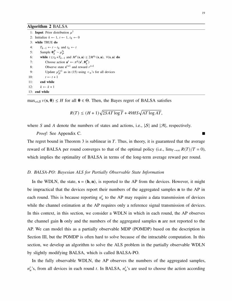
Algorithm 2 BALSA1: Input: Prior distribution `1

2: Initialize 𝑘 ← 1, 𝑡 ← 1, 𝑡𝑘 ← 03: while TRUE do4: 𝑇𝑘−1 ← 𝑡 − 𝑡𝑘 and 𝑡𝑘 ← 𝑡

5: Sample 𝛉𝑃𝑘∼ `𝑡𝑘

𝑃

6: while 𝑡 ≤ 𝑡𝑘 +𝑇𝑘−1 and 𝑀 𝑡 (s, a) ≤ 2𝑀 𝑡𝑘 (s, a), ∀(s, a) do7: Choose action a𝑡 ← 𝜋𝑔 (s𝑡 , 𝛉𝑃

𝑘)

8: Observe state s𝑡+1 and reward 𝑟 𝑡+1

9: Update `𝑡+1𝑃

as in (15) using 𝑚𝑢’s for all devices10: 𝑡 ← 𝑡 + 111: end while12: 𝑘 ← 𝑘 + 113: end while

max𝑠∈S 𝑣(s, 𝛉) ≤ 𝐻 for all 𝛉 ∈ Θ. Then, the Bayes regret of BALSA satisfies

𝑅(𝑇) ≤ (𝐻 + 1)√

2𝑆𝐴𝑇 log𝑇 + 49𝐻𝑆√𝐴𝑇 log 𝐴𝑇,

where 𝑆 and 𝐴 denote the numbers of states and actions, i.e., |S| and |A|, respectively.

Proof: See Appendix C.

The regret bound in Theorem 3 is sublinear in 𝑇 . Thus, in theory, it is guaranteed that the average

reward of BALSA per round converges to that of the optimal policy (i.e., lim𝑇→∞ 𝑅(𝑇)/𝑇 = 0),

which implies the optimality of BALSA in terms of the long-term average reward per round.

D. BALSA-PO: Bayesian ALS for Partially Observable State Information

In the WDLN, the state, s = (h, n), is reported to the AP from the devices. However, it might

be impractical that the devices report their numbers of the aggregated samples n to the AP in

each round. This is because reporting 𝑛𝑡𝑢 to the AP may require a data transmission of devices

while the channel estimation at the AP requires only a reference signal transmission of devices.

In this context, in this section, we consider a WDLN in which in each round, the AP observes

the channel gain h only and the numbers of the aggregated samples n are not reported to the

AP. We can model this as a partially observable MDP (POMDP) based on the description in

Section III, but the POMDP is often hard to solve because of the intractable computation. In this

section, we develop an algorithm to solve the ALS problem in the partially observable WDLN

by slightly modifying BALSA, which is called BALSA-PO.

In the fully observable WDLN, the AP observes the numbers of the aggregated samples,

𝑛𝑡𝑢’s, from all devices in each round 𝑡. In BALSA, 𝑛𝑡𝑢’s are used to choose the action according

20

TABLE IVCOMPARISON OF COMPUTATIONAL COMPLEXITY

Computational complexity up to round 𝑇

DP-based with perfect information 𝑂 (𝑆2𝐴)

DP-based without informationUpper-bound: 𝑂 (𝑆2𝐴𝑇 )Lower-bound: 𝑂 (

√𝑆3𝐴𝑇 (log𝑇 )−1)

ALSA-PI,BALSA(-PO) 𝑂 (𝑈𝑇 log𝑈 )𝑆 = |S | = ( |H | |N |)𝑈 and 𝐴 = |A | = 𝑈!

𝑊 !(𝑈−𝑊 ) !

to the greedy policy in (14) and to obtain the numbers of the arrived samples of all devices

during round 𝑡 − 1, 𝑚𝑡−1𝑢 ’s, for updating the posterior distribution of \𝑃𝑢 . Hence, in the partially

observable WDLN, where 𝑛𝑡𝑢’s are not observable, the AP cannot choose the action according to

the greedy policy as well as obtain 𝑚𝑡−1𝑢 ’s. To address these issues, first, in BALSA-PO, the AP

approximates 𝑛𝑡𝑢 by using the sampled parameter of \𝑃𝑢 as ��𝑡𝑢 = (𝑇𝑛𝑢 − 1)\𝑃𝑢,𝑘

, where 𝑇𝑛𝑢 is the

number of the rounds from the latest successful local update transmission to the current round

(i.e., 𝑇𝑛𝑢 = 𝑡 −max{𝜏 < 𝑡 : 𝑥𝜏𝑢 = 1 and 𝑎𝜏𝑢 = 1}) and \𝑃𝑢,𝑘

is the sampled parameter of \𝑃𝑢 in stage

𝑘 . Then, the AP can choose the action according to the greedy policy by using the approximated

𝑛𝑡𝑢’s, i.e., ��𝑡𝑢. However, the chosen action will be meaningful only if the posterior distribution

keeps updated correctly since 𝑛𝑡𝑢’s are approximated based on the samples parameters. In the

partially observable WDLN, it is a challenging issue updating the posterior distribution correctly

since the AP cannot obtain 𝑚𝑡𝑢’s which are required to update the posterior distribution. However,

fortunately, even in the partially observable WDLN, the AP can still observe the information

about the number of samples 𝑛𝑡𝑢 + 𝑚𝑡𝑢 in every successful local update transmission since the

information is included in the local update transmission (line 7 of Algorithm 1). Note that 𝑛𝑡𝑢 +𝑚𝑡𝑢denotes the sum of 𝑚𝑡𝑢’s over the rounds from the latest successful local update transmission

to the current round. This sum of 𝑚𝑡𝑢’s in the partially observable WDLN is less informative

than all individual values of 𝑚𝑡𝑢’s. Nevertheless, it is informative enough to update the posterior

distribution because the update of the posterior distribution of \𝑃𝑢 requires only the sum of 𝑚𝑡𝑢’s as

in (15). Hence, in the partially observable WDLN, the AP can update the posterior distribution of

\𝑃𝑢 when device 𝑢 successfully transmits its local update. Then, BALSA-PO can be implemented

by substituting the state in BALSA, s, to s = (h, n), where n = {��1, ..., ��𝑈} and changing the

posterior distribution update procedure from BALSA in line 9 of Algorithm 2 as follows: “Update

`𝑡+1\𝑃𝑢

as in (15) using 𝑛𝑡𝑢 + 𝑚𝑡𝑢 for device 𝑢 ∈ U𝑡”.

21

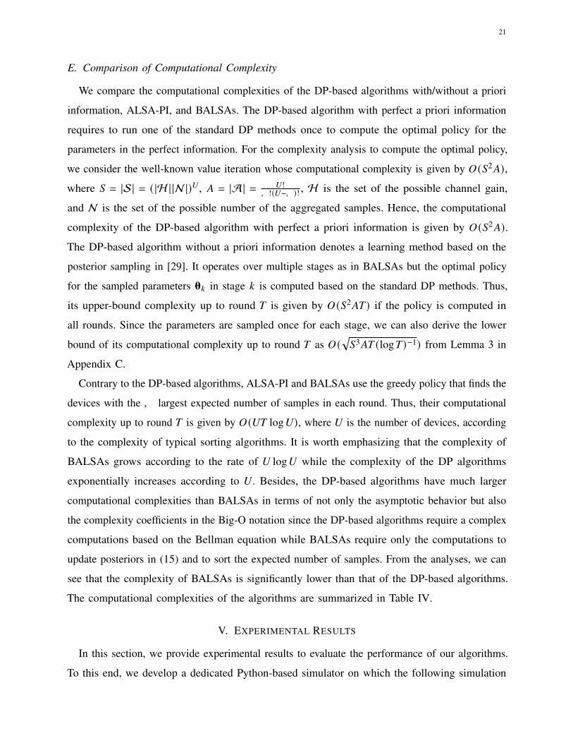
E. Comparison of Computational Complexity

We compare the computational complexities of the DP-based algorithms with/without a priori

information, ALSA-PI, and BALSAs. The DP-based algorithm with perfect a priori information

requires to run one of the standard DP methods once to compute the optimal policy for the

parameters in the perfect information. For the complexity analysis to compute the optimal policy,

we consider the well-known value iteration whose computational complexity is given by 𝑂 (𝑆2𝐴),where 𝑆 = |S| = ( |H ||N |)𝑈 , 𝐴 = |A| = 𝑈!

𝑊!(𝑈−𝑊)! , H is the set of the possible channel gain,

and N is the set of the possible number of the aggregated samples. Hence, the computational

complexity of the DP-based algorithm with perfect a priori information is given by 𝑂 (𝑆2𝐴).The DP-based algorithm without a priori information denotes a learning method based on the

posterior sampling in [29]. It operates over multiple stages as in BALSAs but the optimal policy

for the sampled parameters 𝛉𝑘 in stage 𝑘 is computed based on the standard DP methods. Thus,

its upper-bound complexity up to round 𝑇 is given by 𝑂 (𝑆2𝐴𝑇) if the policy is computed in

all rounds. Since the parameters are sampled once for each stage, we can also derive the lower

bound of its computational complexity up to round 𝑇 as 𝑂 (√𝑆3𝐴𝑇 (log𝑇)−1) from Lemma 3 in

Appendix C.

Contrary to the DP-based algorithms, ALSA-PI and BALSAs use the greedy policy that finds the

devices with the 𝑊 largest expected number of samples in each round. Thus, their computational

complexity up to round 𝑇 is given by 𝑂 (𝑈𝑇 log𝑈), where 𝑈 is the number of devices, according

to the complexity of typical sorting algorithms. It is worth emphasizing that the complexity of

BALSAs grows according to the rate of 𝑈 log𝑈 while the complexity of the DP algorithms

exponentially increases according to 𝑈. Besides, the DP-based algorithms have much larger

computational complexities than BALSAs in terms of not only the asymptotic behavior but also

the complexity coefficients in the Big-O notation since the DP-based algorithms require a complex

computations based on the Bellman equation while BALSAs require only the computations to

update posteriors in (15) and to sort the expected number of samples. From the analyses, we can

see that the complexity of BALSAs is significantly lower than that of the DP-based algorithms.

The computational complexities of the algorithms are summarized in Table IV.

V. EXPERIMENTAL RESULTS

In this section, we provide experimental results to evaluate the performance of our algorithms.

To this end, we develop a dedicated Python-based simulator on which the following simulation

22

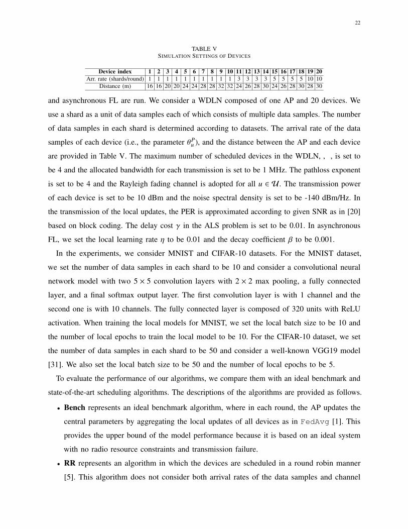
TABLE VSIMULATION SETTINGS OF DEVICES

Device index 1 2 3 4 5 6 7 8 9 10 11 12 13 14 15 16 17 18 19 20Arr. rate (shards/round) 1 1 1 1 1 1 1 1 1 1 3 3 3 3 5 5 5 5 10 10

Distance (m) 16 16 20 20 24 24 28 28 32 32 24 26 28 30 24 26 28 30 28 30

and asynchronous FL are run. We consider a WDLN composed of one AP and 20 devices. We

use a shard as a unit of data samples each of which consists of multiple data samples. The number

of data samples in each shard is determined according to datasets. The arrival rate of the data

samples of each device (i.e., the parameter \𝑃𝑢 ), and the distance between the AP and each device

are provided in Table V. The maximum number of scheduled devices in the WDLN, 𝑊 , is set to

be 4 and the allocated bandwidth for each transmission is set to be 1 MHz. The pathloss exponent

is set to be 4 and the Rayleigh fading channel is adopted for all 𝑢 ∈ U. The transmission power

of each device is set to be 10 dBm and the noise spectral density is set to be -140 dBm/Hz. In

the transmission of the local updates, the PER is approximated according to given SNR as in [20]

based on block coding. The delay cost 𝛾 in the ALS problem is set to be 0.01. In asynchronous

FL, we set the local learning rate [ to be 0.01 and the decay coefficient 𝛽 to be 0.001.

In the experiments, we consider MNIST and CIFAR-10 datasets. For the MNIST dataset,

we set the number of data samples in each shard to be 10 and consider a convolutional neural

network model with two 5 × 5 convolution layers with 2 × 2 max pooling, a fully connected

layer, and a final softmax output layer. The first convolution layer is with 1 channel and the

second one is with 10 channels. The fully connected layer is composed of 320 units with ReLU

activation. When training the local models for MNIST, we set the local batch size to be 10 and

the number of local epochs to train the local model to be 10. For the CIFAR-10 dataset, we set

the number of data samples in each shard to be 50 and consider a well-known VGG19 model

[31]. We also set the local batch size to be 50 and the number of local epochs to be 5.

To evaluate the performance of our algorithms, we compare them with an ideal benchmark and

state-of-the-art scheduling algorithms. The descriptions of the algorithms are provided as follows.

• Bench represents an ideal benchmark algorithm, where in each round, the AP updates the

central parameters by aggregating the local updates of all devices as in FedAvg [1]. This

provides the upper bound of the model performance because it is based on an ideal system

with no radio resource constraints and transmission failure.

• RR represents an algorithm in which the devices are scheduled in a round robin manner

[5]. This algorithm does not consider both arrival rates of the data samples and channel

23

0 20 40 60 80 100

Round

-200

-100

0

100

200

Effe

ctivity s

co

re

RR

W-maxALSA-PI

BALSA

BALSA-PO

Fig. 2. Average effectivity score of the ALS problem achieved by the algorithms.

information of the devices.

• 𝑊-max represents an algorithm that schedules the devices who have the 𝑊 strongest channel

gains. This algorithm does not consider the arrival rates of the data samples. It can represent

the scheduling strategies in [7], [9].

• ALSA-PI is implemented as described in Section IV-B to schedule the devices according

to the greedy policy in (14) with the perfect a priori information about 𝛉∗,𝑃.

• BALSA is implemented as Algorithm 2 in Section IV-C for the fully observable WDLN.

For the Bayesian approach, the Jeffreys prior is used.

• BALSA-PO is implemented as described in Section IV-D. The Jeffreys prior is used as in

BALSA. This algorithm is for the partially observable WDLN.

The models are trained by asynchronous FL with above transmission scheduling algorithms. We

run 50 simulation instances for MNIST dataset and 20 simulation instances for CIFAR-10 dataset.

In the following figures, the 95% confidence interval is illustrated as a shaded region.

A. Effectivity Scores in the ALS Problem

We first provide the effectivity scores of the algorithms, which are the objective function of the

ALS problem in (11), in Fig. 2. Note that Bench is not provided in the figure since in Bench, all

devices transmit their local updates and all the transmissions succeed. From the figure, we can see

that our BALSAs achieve the similar effectivity score to that of ALSA-PI, which is the optimal

one. In particular, as the round proceeds, the effectivity scores of BALSAs converge to that of

ALSA-PI. This clearly shows that our BALSAs can effectively learn the uncertainties in the

WDLN. On the other hand, RR and 𝑊-max achieve the much lower effectivity scores compared

with BALSAs. Especially, the effectivity score of 𝑊-max decreases as the round proceeds since

it fails not only to maximize the number of the data samples used in training and but also to

24

Bench RR W-max ALSA-PI BALSA BALSA-PO

0 50 100

Round

0

10

20

30

Lo

ss

(a) Training loss with MNIST

0 50 100

Round

0.6

0.7

0.8

0.9

1

Accu

racy

(b) Test accuracy with MNIST

0 50 100

Round

10

20

30

40

50

60

Lo

ss

(c) Training loss with CIFAR-10

0 50 100

Round

0.2

0.4

0.6

0.8

Accu

racy

(d) Test accuracy with CIFAR-10

Fig. 3. Training loss and test accuracy with MNIST and CIFAR-10 datasets.

minimize the adverse effect from the stragglers. To show the validity of the effectivity score for

effective learning in asynchronous FL, in the following subsections, it will be clearly shown that

the algorithms with the higher effectivity scores achieve better trained model performances such

as training loss, accuracy, robustness against stragglers, and learning speed.

B. Training Loss and Test Accuracy

To compare the performance of asynchronous FL with respect to the transmission scheduling

algorithms, which is our ultimate goal, we provide the training loss and test accuracy of the

algorithms. Fig. 3 provides the training loss and test accuracy with MNIST and CIFAR-10 datasets.

From Figs. 3a and 3c, we can see that ALSA-PI, BALSA, and BALSA-PO achieve the similar

training loss to Bench. Compared with them, RR and 𝑊-max achieve the larger training loss. The

larger training loss of a model typically implies the lower accuracy of the model. This is clearly

shown in Figs. 3b and 3d. From the figures, we can see that the models trained with RR and

𝑊-max achieve the significantly lower accuracy than the models trained with the other algorithms

and their variances are much larger than those of the other algorithms. These results imply

that RR and 𝑊-max fail to effectively gather the local updates while addressing the stragglers

because they do not have a capability to consider the characteristics of asynchronous FL and the

uncertainties in the WDLN. On the other hand, our BALSAs gather the local updates which are

enough to train the model while effectively addressing the stragglers due to asynchronous FL by

considering the effectivity score.

C. Robustness of Learning against Stragglers

In Fig. 3, the unstable learning of the algorithms due to the stragglers is not clearly shown

since the fluctuations of the training loss and accuracy in the figure are wiped out while averaging

25

Bench RR W-max ALSA-PI BALSA BALSA-PO

0 50 100

Round

0

10

20

30

40

50

Lo

ss

(a) Training loss with MNIST

0 50 100

Round

0.4

0.6

0.8

1

Accu

racy

(b) Test accuracy with MNIST

0 50 100

Round

0

20

40

60

80

100

Lo

ss

(c) Training loss with CIFAR-10

0 50 100

Round

0

0.2

0.4

0.6

0.8

Accu

racy

(d) Test accuracy with CIFAR-10

Fig. 4. Training loss and test accuracy of a single simulation instance with MNIST and CIFAR-10 datasets.

Bench RR W-max ALSA-PI BALSA BALSA-PO

0.7 0.75 0.8 0.85 0.9 0.95

Target accuracy

0.8

0.9

1

Satisfa

ction r

ate

(a) Target accuracy satisfactionrate with MNIST

0.7 0.75 0.8 0.85 0.9 0.95

Target accuracy

0

20

40

60

Avera

ge r

ound

(b) Average required roundswith MNIST

0.5 0.55 0.6 0.65 0.7 0.75

Target accuracy

0

0.2

0.4

0.6

0.8

1

Satisfa

ction r

ate

(c) Target accuracy satisfactionrate with CIFAR-10

0.5 0.55 0.6 0.65 0.7 0.75

Target accuracy

20

40

60

80

Avera

ge r

ound

(d) Average required roundswith CIFAR-10

Fig. 5. Target accuracy satisfaction rate and average required rounds for satisfying the target accuracy with MNIST and CIFAR-10datasets.

the results from the multiple simulation instances. Hence, in Fig. 4, we show the robustness

of the algorithms against the stragglers more clearly through the training loss and test accuracy

results of a single simulation instance. First of all, it is worth emphasizing that Bench is the most

stable one in terms of the stragglers because it has no straggler. From Figs. 4a and 4c, we can see

that the training losses of the algorithms considering asynchronous FL based on the effectivity

score (i.e., ALSA-PI and BALSAs) are quite stable as much as that of Bench. Accordingly,

their corresponding test accuracies are also stable. On the other hand, for the algorithms not

considering asynchronous FL (i.e., RR and 𝑊-max), a lot of spikes (i.e., short-lasting peaks)

appear in their training losses, and accordingly, their test accuracies are also unstable. Moreover,

the training loss and test accuracy of 𝑊-max is significantly unstable compared with RR. This

is because the scheduling strategy of 𝑊-max is highly biased according to the average channel

gain while RR sequentially schedules all the devices. Such biased scheduling in 𝑊-max raises

much more stragglers than RR. This clearly shows that a transmission scheduling algorithm may

cause unstable learning if its scheduling strategy is biased without considering the stragglers.

26

D. Satisfaction Rate and Learning Speed

In Fig. 5, we provide the target accuracy satisfaction rate and the average required rounds

for satisfying the target accuracy of each algorithm. For the MNIST dataset, we vary the target

accuracy from 0.7 to 0.95, and for the CIFAR-10 dataset, we vary it from 0.5 to 0.75. The test

accuracy satisfaction rate of each algorithm is obtained as the ratio of the simulation instances,

where the test accuracy of the corresponding trained model exceeds the target accuracy at the

end of the simulation, to the total simulation instances. For the average required rounds for

satisfying the target accuracy, we find the minimum required rounds of each simulation instance

in which the target accuracy is satisfied. To avoid the effect of the spikes, we set a criteria of

satisfying the target accuracy as follows: all test accuracies in three consecutive rounds exceed

the target accuracy. From Figs. 5a and 5c, we can see that the satisfaction rates of ALSA-PI and

BALSAs are similar to that of Bench. On the other hand, the satisfaction rates of RR and 𝑊-max

significantly decrease as the target accuracy increases. Figs. 5b and 5d provide the average

required rounds of the algorithms to satisfy the target accuracy. From the figures, we can see

that the algorithms considering asynchronous FL (ALSA-PI and BALSAs) require the smaller

rounds to satisfy the target accuracy. This clearly shows that the algorithms that consider the

effective score of asynchronous FL (i.e., ALSA-PI and BALSAs) have a faster learning speed

than the algorithms that do not consider it (i.e., RR and 𝑊-max).

VI. CONCLUSION AND FUTURE WORK

In this paper, we proposed the asynchronous FL procedure in the WDLN and investigated its

convergence. We also investigated transmission scheduling in the WDLN for effective learning.

To this end, we first proposed the effectivity score of asynchronous FL that represents the amount

of learning in which the harmful effects on learning due to the stragglers are considered. We

then formulated the ALS problem that maximizes the effectivity score of asynchronous FL. We

developed ALSA-PI that can solve the ALS problem when the perfect a priori information is

given. We also developed BALSA and BALSA-PO that effectively solve the ALS problem without

a priori information by learning the uncertainty on stochastic data arrivals with a minimal amount

of information. Our experimental results show that our ALSA-PI and BALSAs achieve the similar

performance to the ideal benchmark. In addition, they outperform the other baseline scheduling

algorithms. These results clearly show that the transmission scheduling strategy based on the

effectivity score, which is adopted to our algorithms, is effective for asynchronous FL. Besides,

27

our BALSAs effectively schedules the transmissions even without any a priori information by

learning the system uncertainties. As a future work, a non-i.i.d. distribution of data samples over

devices can be incorporated into the ALS problem for more effective learning in a non-i.i.d. data

distribution scenario. In addition, subchannel allocation and power control can be considered

as well to utilize the resources more effectively.

APPENDIX A

PROOF OF THEOREM 1

We first provide the following lemma to prove Theorem 1.

Lemma 1: [11] If 𝑙 (w) is b-strong convex, then with Assumption 1, we have

2b (𝑙 (w𝑡) − 𝑙 (w∗)) ≤ ||∇𝑙 (w𝑡) | |2.

Using Lemma 1, we now prove Theorem 1. Since 𝑙 (w) is 𝐿-smooth, the following holds:

𝑙 (w𝑡+1) − 𝑙 (w𝑡) ≤⟨∇𝑙 (w𝑡),w𝑡+1 − w𝑡

⟩+ 𝐿

2‖w𝑡+1 − w𝑡 ‖2

= −∑𝑢∈U𝑡

∇𝑙 (w𝑡)>[𝑡𝑢𝑐𝑡𝑢𝜓𝑡𝑢 +𝐿

2

∑𝑢∈U𝑡

[𝑡𝑢𝑐𝑡𝑢𝜓

𝑡𝑢

2.

≤ −∑𝑢∈U𝑡

∇𝑙 (w𝑡)>[𝑡𝑢𝑐𝑡𝑢𝜓𝑡𝑢 +𝐿

2

( ∑𝑢∈U𝑡

| |[𝑡𝑢𝑐𝑡𝑢𝜓𝑡𝑢 | |)2.

Let us define 𝑞 = max𝑢∈U{[𝑡𝑢𝑐𝑡𝑢}. Then, 𝑞 > 0 and with Assumption 1 and gradient dissimilarity,

the following holds:

E[𝑙 (w𝑡+1)] − 𝑙 (w𝑡) ≤ −𝑞∑𝑢∈U𝑡

∇𝑙 (w𝑡)E[𝜓𝑡𝑢] +𝐿𝑞2

2E[ ∑𝑢∈U𝑡

| |𝜓𝑡𝑢 | |]2

≤ −𝑞𝑈𝜖 | |∇𝑙 (w𝑡) | |2 + 𝐿𝑞2𝑈2𝑉2

2| |∇𝑙 (w𝑡) | |2

= −𝑞𝑈(𝜖 − 𝐿𝑞𝑈𝑉

2

2

)| |∇𝑙 (w𝑡) | |2. (16)

Let us define [𝑡 = max𝑢∈U [𝑡𝑢. Then, we have −𝑞𝑈(𝜖 − 𝐿𝑞𝑈𝑉2

2

)< −[𝑡𝑈

(𝜖 − 𝐿[𝑡𝑈𝑉2

2

)because

𝑐𝑡𝑢 < 0 for all 𝑢, 𝑡. Now, with Lemma 1, we can rewrite the inequality in (16) as

E[𝑙 (w𝑡+1)] − 𝑙 (w𝑡) ≤ −2b[𝑡𝑈𝜖′′(𝑙 (w𝑡) − 𝑙 (w∗)),

where 𝜖′′ = 𝜖− 𝐿[𝑡𝑈𝑉2

2 . By subtracting 𝑙 (w∗) from both sides and rearranging the inequality, we have

E[𝑙 (w𝑡+1)] − 𝑙 (w∗) ≤ (1 − 2b[𝑡𝑈𝜖′′) (𝑙 (w𝑡) − 𝑙 (w∗)).

28

By taking expectation of both sides, we can get

E[𝑙 (w𝑡+1) − 𝑙 (w∗)] ≤ (1 − 2b[𝑈𝜖′) (𝑙 (w𝑡) − 𝑙 (w∗)),

where 𝜖′ = 𝜖 − 𝐿[𝑡𝑈𝑉2

2 and [𝑡 = 2𝜖𝐿𝑈𝑉2 (max𝑢∈U{𝑐𝑡𝑢})−1. With telescoping the above equations, we

have Theorem 1.

APPENDIX B

PROOF OF THEOREM 2

Suppose that there exists the optimal policy whose chosen action in a round with state s is not

identical to the greedy policy. We denote the expected instantaneous effectivity score of round 𝑡

with the optimal policy by 𝑟 𝑡∗(s) and that with the greedy policy by 𝑟 𝑡𝑔 (s). Based on the equation in

(13), we can decompose the expected instantaneous effectivity score into two sub-rewards as 𝑟 (s) =𝑟𝐴 (s) +𝑟𝐵 (s), where 𝑟𝐴 (s) = E[

∑𝑢∈U 𝑎𝑢𝑥𝑢 (1+𝛾) (𝑛𝑢+𝑚𝑢)] and 𝑟𝐵 (s) = −E[

∑𝑢∈U 𝛾(𝑛𝑢+𝑚𝑢)]. In

the problem, the samples are accumulated if they are not used for central training. Moreover, the

channel gains and arrival rates of the samples of the devices are i.i.d. Hence, if a policy 𝜋 satisfies∑𝑠∈SP[𝑎𝜋𝑢 (s)] > 0 for all 𝑢 ∈ U, (17)

where 𝑎𝜋𝑢 represents 𝑎𝑢 from policy 𝜋, any arrived samples will be eventually reflected in the

sub-reward 𝑟𝐴 regardless of the policy due to the accumulation of the samples. This implies that

the average of sub-reward∑𝑇𝑡=1 𝑟

𝑡𝐴/𝑇 converges to

∑𝑢∈U \

𝑃𝑢 as 𝑇 →∞. Accordingly, if a policy

satisfies the condition in (17), its optimality to the ALS problem depends on minimizing the delay

cost (i.e., the sub-reward 𝑟𝐵). With the greedy policy, any device will be scheduled when the

number of its aggregated samples is large enough. Hence, the greedy policy satisfies the condition

if the parameters are finite. We now denote the expected sub-rewards 𝑟𝐵 of round 𝑡 with the optimal

policy and the greedy policy by 𝑟 𝑡𝐵,∗ and 𝑟 𝑡

𝐵,𝑔, respectively. From the definition of the greedy policy,

it is obvious that E[∑𝑢∈U 𝑛𝑡𝑢 |a∗] ≥ E[

∑𝑢∈U 𝑛

𝑡𝑢 |a𝑔], which implies that 𝑟 𝑡

𝐵,∗ ≤ 𝑟𝑡𝐵,𝑔, for any random

disturbances. Consequently, this leads to 𝐽∗ ≤ 𝐽𝑔, which implies that the greedy policy is optimal.

APPENDIX C

PROOF OF THEOREM 3

We first define 𝐾𝑇 = argmax{𝑘 : 𝑡𝑘 ≤ 𝑇}, which represents the number of stages in BALSA

until round 𝑇 . For 𝑡𝑘 ≤ 𝑡 < 𝑡𝑘+1 in stage 𝑘 , we have the following equation from the Bellman

29

equation in (12):

𝑟 (s𝑡 , a𝑡) = 𝐽 (𝛉𝑘 ) + 𝑣(s𝑡 , 𝛉𝑘 ) −∑s′∈S

𝑃𝛉𝑘 (s′|s𝑡 , a𝑡)𝑣(s′, 𝛉𝑘 ).

Then, the expected regret of BALSA is derived as

𝑇E[𝐽 (𝛉∗)] − E[ 𝐾𝑇∑𝑘=1

𝑡𝑘+1−1∑𝑡=𝑡𝑘

𝑟 (s𝑡 , a𝑡)]= 𝑅1 + 𝑅2 + 𝑅3, (18)

where 𝑅1 = 𝑇E[𝐽 (𝛉∗)] −E[ ∑𝐾𝑇

𝑘=1 𝑇𝑘𝐽 (𝛉𝑘 )], 𝑅2 = E

[ ∑𝐾𝑇

𝑘=1∑𝑡𝑘+1−1𝑡=𝑡𝑘

𝑣(s𝑡+1, 𝛉𝑘 ) − 𝑣(s𝑡 , 𝛉𝑘 )], and

𝑅3 = E[ ∑𝐾𝑇

𝑘=1∑𝑡𝑘+1−1𝑡=𝑡𝑘

∑s′∈S 𝑃

𝛉𝑘 (s′|s𝑡 , a𝑡)𝑣(s′, 𝛉𝑘 ) − 𝑣(s𝑡+1, 𝛉𝑘 )]. We can bound the regret of

BALSA by deriving the bounds on 𝑅1, 𝑅2, and 𝑅3 as the following lemma:

Lemma 2: For the expected regret of BALSA, we have the following bounds:

• The first term is bounded as 𝑅1 ≤ E[𝐾𝑇 ].• The second term is bounded as 𝑅2 ≤ E[𝐻𝐾𝑇 ].• The third term is bounded as 𝑅3 ≤ 49𝐻𝑆

√𝐴𝑇 log(𝐴𝑇).

In addition, we can bound the number of stages 𝐾𝑇 as follows.

Lemma 3: The number of stages in BALSA until round 𝑇 is bounded as 𝐾𝑇 ≤√

2𝑆𝐴𝑇 log(𝑇).We can prove above lemmas in similar steps to Lemmas 1–5 in [29]. Hence, here we omit the

proofs due to the lack of space. From the equation in (18), we have 𝑅(𝑇) = 𝑅1 + 𝑅2 + 𝑅3. Then,

Theorem 3 holds by Lemmas 2 and 3.

REFERENCES

[1] B. McMahan, E. Moore, D. Ramage, S. Hampson, and B. A. y Arcas, “Communication-efficient learning of deep networks

from decentralized data,” in Proc. AISTATS, 2017.

[2] W. Y. B. Lim, N. C. Luong, D. T. Hoang, Y. Jiao, Y.-C. Liang, Q. Yang, D. Niyato, and C. Miao, “Federated learning in

mobile edge networks: A comprehensive survey,” IEEE Commun. Surveys Tuts., no. 3, pp. 2031–2063, 2020.

[3] M. M. Amiri and D. Gündüz, “Federated learning over wireless fading channels,” IEEE Trans. Wireless Commun., vol. 19,

no. 5, pp. 3546–3557, May 2020.

[4] ——, “Machine learning at the wireless edge: Distributed stochastic gradient descent over-the-air,” IEEE Trans. Signal

Process., vol. 68, pp. 2155–2169, Mar. 2020.

[5] H. H. Yang, Z. Liu, T. Q. Quek, and H. V. Poor, “Scheduling policies for federated learning in wireless networks,” IEEE

Trans. Commun., vol. 68, no. 1, pp. 317–333, Jan. 2020.

[6] S. Wang, T. Tuor, T. Salonidis, K. K. Leung, C. Makaya, T. He, and K. Chan, “Adaptive federated learning in resource

constrained edge computing systems,” IEEE J. Sel. Areas Commun., vol. 37, no. 6, pp. 1205–1221, June 2019.

[7] M. M. Amiri, D. Gündüz, S. R. Kulkarni, and H. V. Poor, “Convergence of update aware device scheduling for federated

learning at the wireless edge,” arXiv preprint arXiv:2001.10402, 2020.

30

[8] W. Shi, S. Zhou, Z. Niu, M. Jiang, and L. Geng, “Joint device scheduling and resource allocation for latency constrained

wireless federated learning,” IEEE Trans. Wireless Commun., vol. 20, no. 1, pp. 453–467, Jan. 2021.

[9] M. Chen, Z. Yang, W. Saad, C. Yin, H. V. Poor, and S. Cui, “A joint learning and communications framework for federated

learning over wireless networks,” IEEE Trans. Wireless Commun., vol. 20, no. 1, pp. 269–283, Jan. 2021.

[10] J. Xu and H. Wang, “Client selection and bandwidth allocation in wireless federated learning networks: A long-term

perspective,” IEEE Trans. Wireless Commun., 2020, to be published.

[11] Y. Chen, Y. Ning, M. Slawski, and H. Rangwala, “Asynchronous online federated learning for edge devices with non-IID

data,” arXiv preprint arXiv:1911.02134, 2020.

[12] S. Zheng, Q. Meng, T. Wang, W. Chen, N. Yu, Z.-M. Ma, and T.-Y. Liu, “Asynchronous stochastic gradient descent with

delay compensation,” in Proc. ICML, 2017.

[13] Y. Chen, X. Sun, and Y. Jin, “Communication-efficient federated deep learning with layerwise asynchronous model update

and temporally weighted aggregation,” IEEE Trans. Neural Netw. Learn. Syst., vol. 31, no. 10, pp. 4229–4238, Oct. 2020.

[14] C. Xie, S. Koyejo, and I. Gupta, “Asynchronous federated optimization,” arXiv preprint arXiv:1903.03934, 2020.

[15] T. Chen, G. Giannakis, T. Sun, and W. Yin, “LAG: Lazily aggregated gradient for communication-efficient distributed

learning,” in Proc. NIPS, 2018.

[16] Y. Lin, S. Han, H. Mao, Y. Wang, and B. Dally, “Deep gradient compression: Reducing the communication bandwidth for

distributed training,” in Proc. ICLR, 2018.

[17] J. Xu, W. Du, Y. Jin, W. He, and R. Cheng, “Ternary compression for communication-efficient federated learning,” IEEE

Trans. Neural Netw. Learn. Syst., 2020, to be published.

[18] V. Smith, C.-K. Chiang, M. Sanjabi, and A. S. Talwalkar, “Federated multi-task learning,” in Proc. NIPS, 2017.

[19] I. M. Baytas, M. Yan, A. K. Jain, and J. Zhou, “Asynchronous multi-task learning,” in IEEE ICDM, 2016.

[20] Y. Xi, A. Burr, J. Wei, and D. Grace, “A general upper bound to evaluate packet error rate over quasi-static fading channels,”

IEEE Trans. Wireless Commun., vol. 10, no. 5, pp. 1373–1377, May 2011.

[21] P. Ferrand, J.-M. Gorce, and C. Goursaud, “Approximations of the packet error rate under quasi-static fading in direct and

relayed links,” EURASIP J. on Wireless Commun. and Netw., vol. 2015, no. 1, p. 12, Jan. 2015.

[22] T. Li, A. K. Sahu, M. Zaheer, M. Sanjabi, A. Talwalkar, and V. Smith, “Federated optimization in heterogeneous networks,”

in Proceedings of Machine Learning and Systems, vol. 2, 2020, pp. 429–450.

[23] Z. Tao and Q. Li, “eSGD: Communication efficient distributed deep learning on the edge,” in USENIX Workshop on Hot

Topics in Edge Computing (HotEdge 18). USENIX Association, 2018.

[24] P. Domingos, “A few useful things to know about machine learning,” Commun. of the ACM, vol. 55, no. 10, pp. 78–87,

2012.

[25] I. Goodfellow, Y. Bengio, A. Courville, and Y. Bengio, Deep learning. MIT press Cambridge, 2016, vol. 1, no. 2.

[26] D. P. Bertsekas, Dynamic programming and optimal control. Athena scientific Belmont, MA, 1995, vol. 1, no. 2.

[27] A. Gopalan and S. Mannor, “Thompson sampling for learning parameterized Markov decision processes,” in Proc. Conf.

on Learn. Theory, 2015.

[28] I. Osband and B. Van Roy, “Why is posterior sampling better than optimism for reinforcement learning?” in Proc. ICML,

2017.

[29] Y. Ouyang, M. Gagrani, A. Nayyar, and R. Jain, “Learning unknown Markov decision processes: A Thompson sampling

approach,” in Proc. NIPS, 2017.

[30] M. Misgiyati and K. Nisa, “Bayesian inference of poisson distribution using conjugate and non-informative priors,” in

Prosiding Seminar Nasional Metode Kuantitatif, no. 1, 2017.

[31] K. Simonyan and A. Zisserman, “Very deep convolutional networks for large-scale image recognition,” in Proc. ICLR, 2015.