Embed Size (px)
Citation preview
AD/AS Models and Macro Policy Debates
Phillips Curve
Adaptive vs. Rational Expectations
Policy Impotency Hypothesis
Ricardian Equivalence
Introduction
In previous models, we assumed the price level P was “stuck” in the short run. This implies a horizontal SRAS curve.
Now, we consider two prominent models of aggregate supply in the short run: Sticky-price model Imperfect-information model
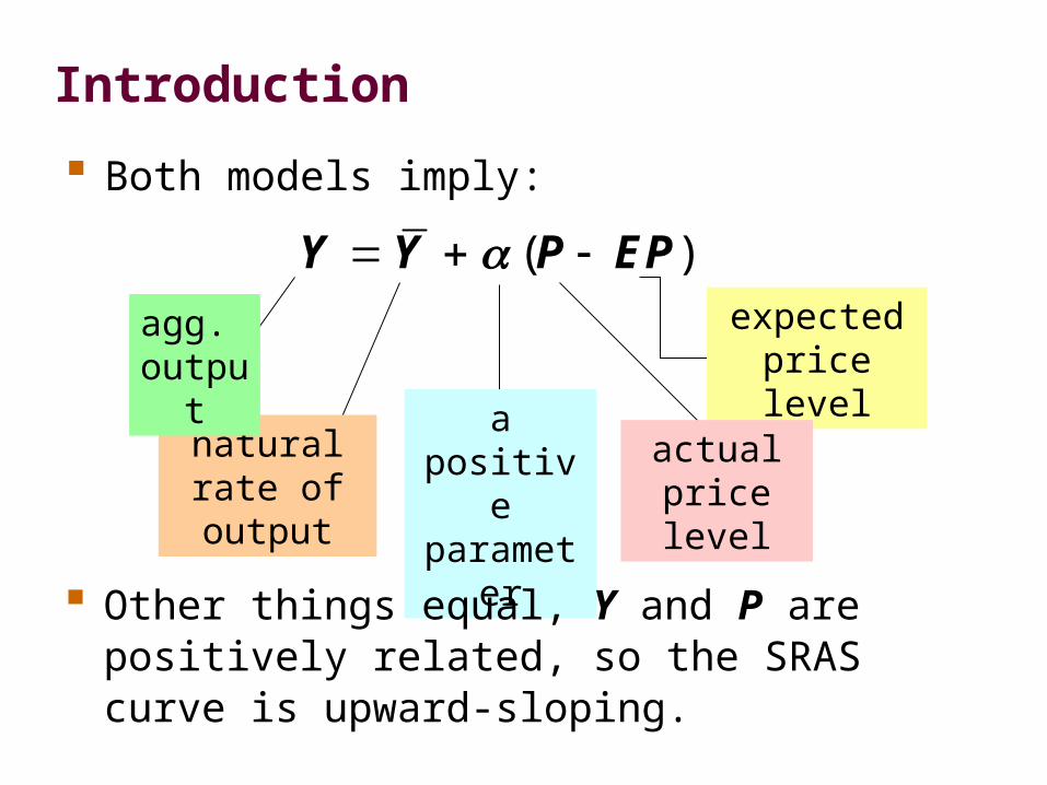
Introduction
Both models imply:
( )Y Y P EP
natural rate of output
a positive parameter
expected price level
actual price level
agg. output
Other things equal, Y and P are positively related, so the SRAS curve is upward-sloping.
The sticky-price model
Reasons for sticky prices: long-term contracts between firms and
customers menu costs firms not wishing to annoy customers with
frequent price changes
Assumption: Firms set their own prices
(i.e., firms have some market power)
The sticky-price model
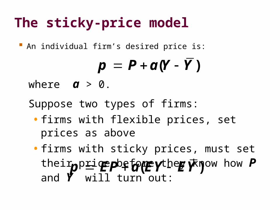
An individual firm’s desired price is:
where a > 0.
Suppose two types of firms:
• firms with flexible prices, set prices as above
• firms with sticky prices, must set their price before they know how P and Y will turn out:
p P a Y Y ( )
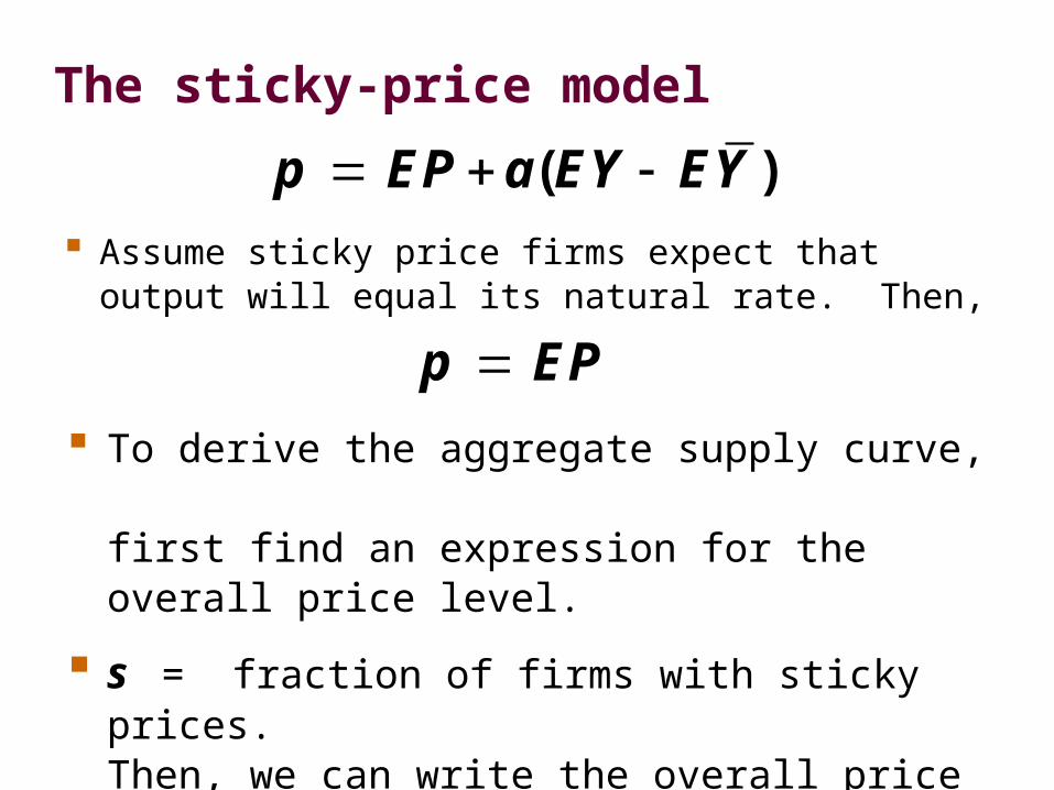
p EP a EY EY ( )
The sticky-price model
Assume sticky price firms expect that output will equal its natural rate. Then,
To derive the aggregate supply curve, first find an expression for the overall price level.
s = fraction of firms with sticky prices. Then, we can write the overall price level as…
p EP a EY EY ( )
p EP
The sticky-price model
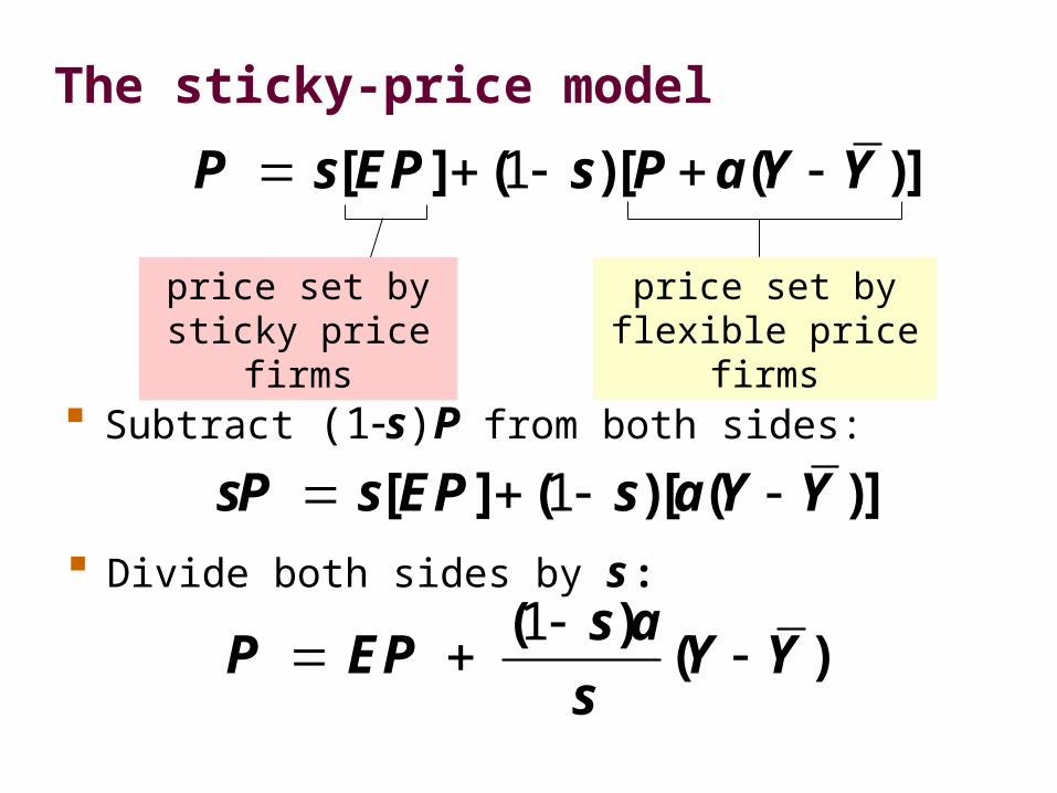
Subtract (1s)P from both sides:
price set by flexible price firms
price set by sticky price firms
Divide both sides by s :
1 [ ] ( )[ ( )]P s EP s P a Y Y
1 [ ] ( )[ ( )]sP s EP s a Y Y
1
( )( )
s aP EP Y Y
s
The sticky-price model
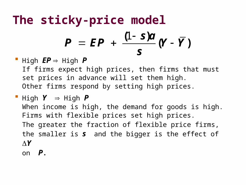
High EP High PIf firms expect high prices, then firms that must set prices in advance will set them high.Other firms respond by setting high prices.
High Y High P When income is high, the demand for goods is high. Firms with flexible prices set high prices. The greater the fraction of flexible price firms, the smaller is s and the bigger is the effect of Y
on P.
1
( )( )
s aP EP Y Y
s
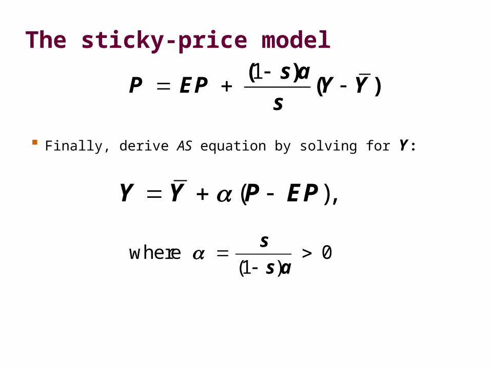
The sticky-price model
Finally, derive AS equation by solving for Y :
( ),Y Y P EP
01
s
s awhere
( )
1
( )( )
s aP EP Y Y
s
The imperfect-information model
Assumptions: All wages and prices are perfectly flexible,
so that all markets clear. Each supplier produces one good, consumes
many goods. Each supplier knows the nominal price of the
good she produces, but does not know the overall price level.
The imperfect-information model Supply of each good depends on its relative
price: the nominal price of the good divided by the overall price level.
Supplier does not know price level at the time she makes her production decision, so uses EP.
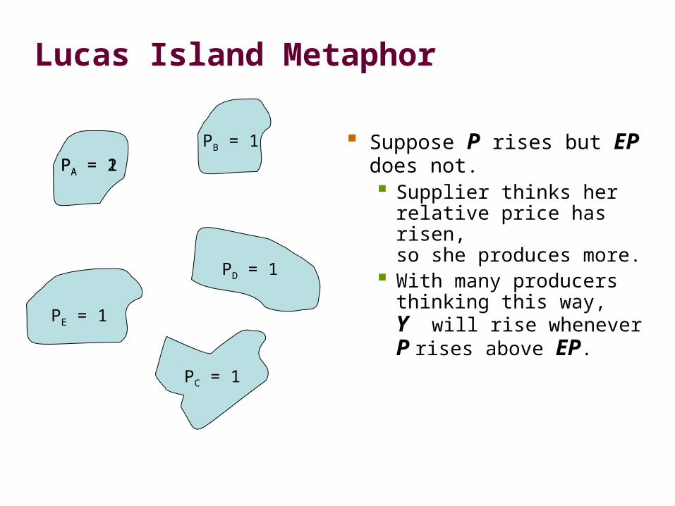
Lucas Island Metaphor
Suppose P rises but EP does not. Supplier thinks her
relative price has risen, so she produces more.
With many producers thinking this way, Y will rise whenever P rises above EP.
PA = 1
PB = 1
PC = 1
PD = 1
PE = 1
PA = 2
Summary & implications
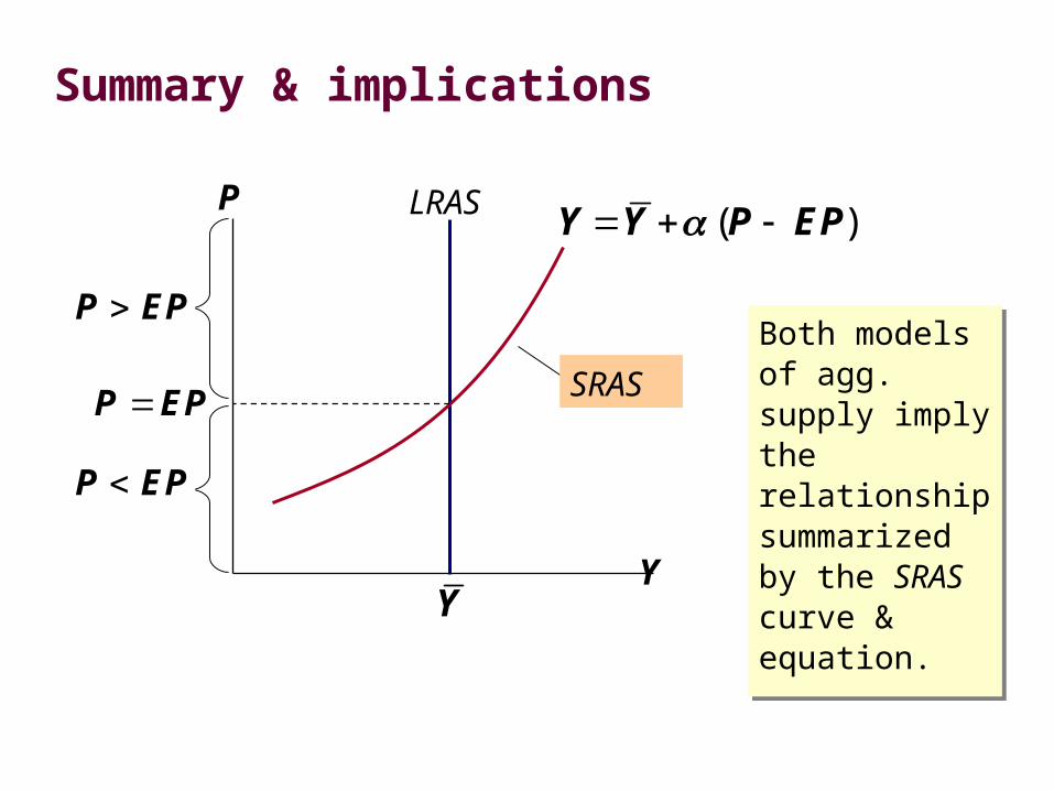
Both models of agg. supply imply the relationship summarized by the SRAS curve & equation.
Both models of agg. supply imply the relationship summarized by the SRAS curve & equation.
Y
P LRAS
Y
SRAS
( )Y Y P EP
P EP
P EP
P EP
Summary & implications
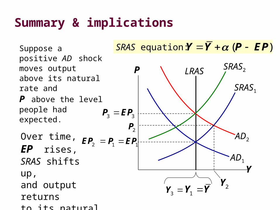
Suppose a positive AD shock moves output above its natural rate and P above the level people had expected.
Y
P LRAS
SRAS1
SRAS equation: ( )Y Y P EP
1 1P EP
AD1
AD22EP
2P3 3P EP
Over time, EP rises, SRAS shifts up,and output returns to its natural rate.
1Y Y 2Y3Y
SRAS2
1960
1961
1962
1963
1964
1965
1966
1967
1968
1969
0.0
0.5
1.0
1.5
2.0
2.5
3.0
3.5
4.0
4.5
5.0
3.0 3.5 4.0 4.5 5.0 5.5 6.0 6.5 7.0
Unemployment Rate
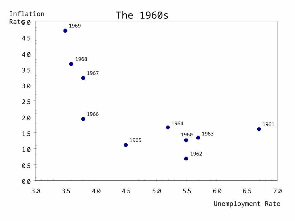
Inflation Rate The 1960s
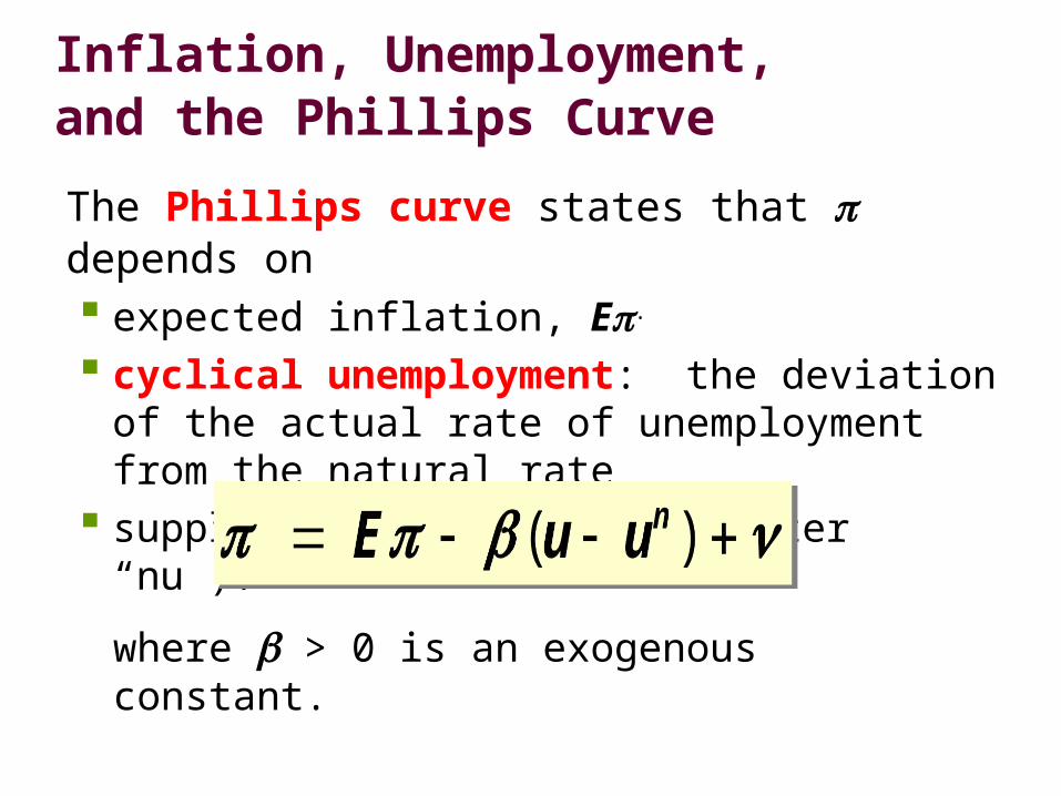
Inflation, Unemployment, and the Phillips Curve
The Phillips curve states that depends on expected inflation, E.
cyclical unemployment: the deviation of the actual rate of unemployment from the natural rate
supply shocks, (Greek letter “nu”).
where > 0 is an exogenous constant.
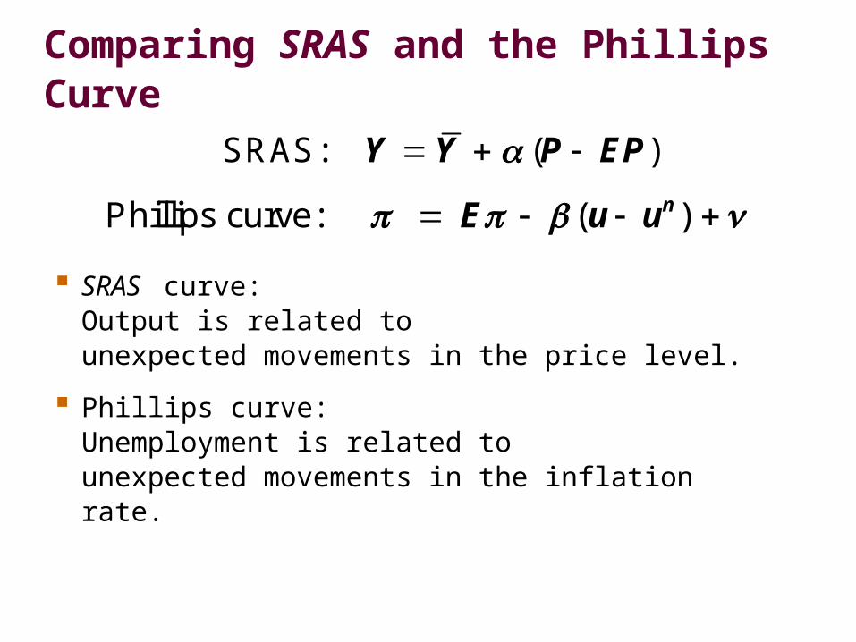
Comparing SRAS and the Phillips Curve
SRAS curve: Output is related to unexpected movements in the price level.
Phillips curve: Unemployment is related to unexpected movements in the inflation rate.
Y Y P EP SRAS: ( )
( )nE u u Phillips curve:
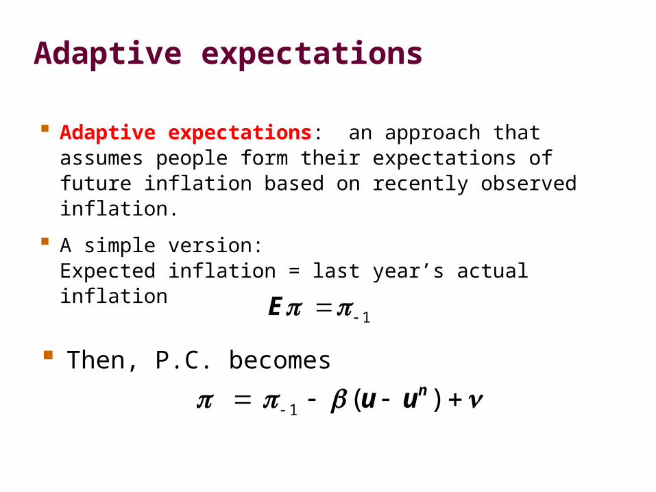
Adaptive expectations
Adaptive expectations: an approach that assumes people form their expectations of future inflation based on recently observed inflation.
A simple version: Expected inflation = last year’s actual inflation
1 ( )nu u
1E
Then, P.C. becomes
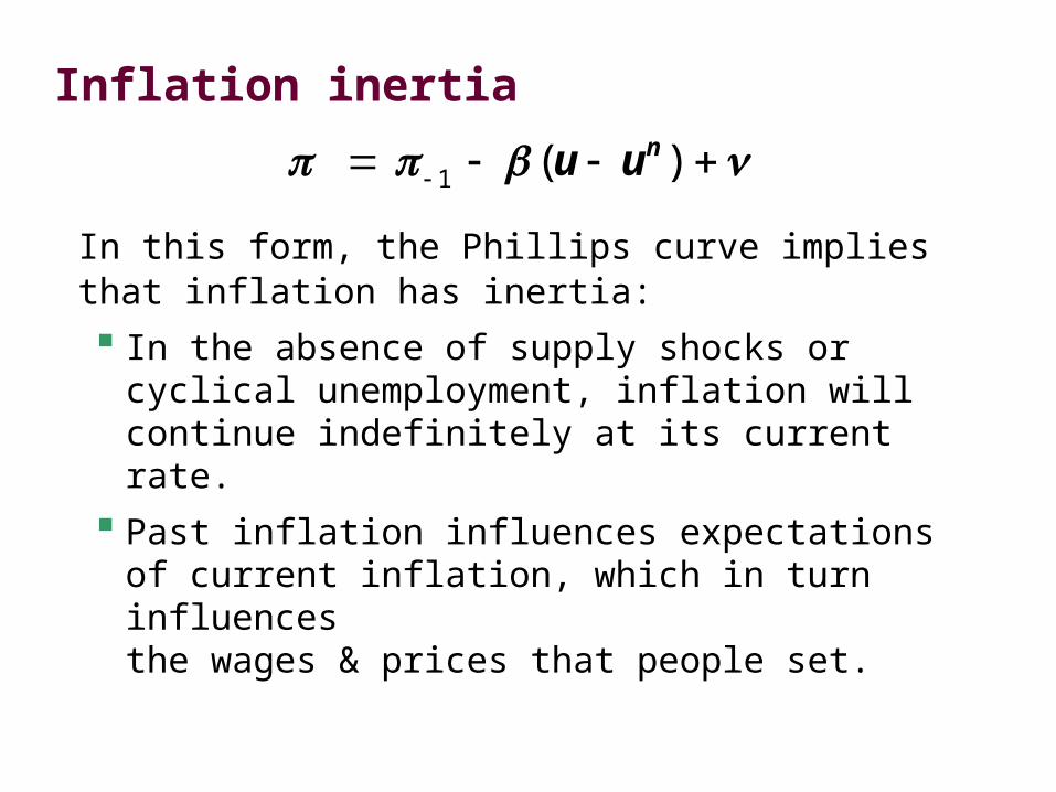
Inflation inertia
In this form, the Phillips curve implies that inflation has inertia:
In the absence of supply shocks or cyclical unemployment, inflation will continue indefinitely at its current rate.
Past inflation influences expectations of current inflation, which in turn influences the wages & prices that people set.
1 ( )nu u
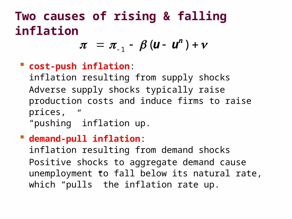
Two causes of rising & falling inflation
cost-push inflation: inflation resulting from supply shocksAdverse supply shocks typically raise production costs and induce firms to raise prices, “pushing” inflation up.
demand-pull inflation: inflation resulting from demand shocksPositive shocks to aggregate demand cause unemployment to fall below its natural rate, which “pulls” the inflation rate up.
1 ( )nu u
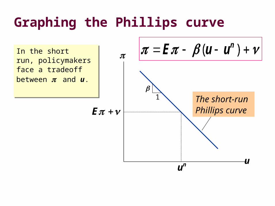
Graphing the Phillips curve
In the short run, policymakers face a tradeoff between and u.
In the short run, policymakers face a tradeoff between and u.
u
nu
1
The short-run Phillips curveE
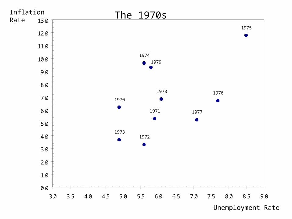
1970
1971
19721973
1974
1975
1976
1977
1978
1979
0.0
1.0
2.0
3.0
4.0
5.0
6.0
7.0
8.0
9.0
10.0
11.0
12.0
13.0
3.0 3.5 4.0 4.5 5.0 5.5 6.0 6.5 7.0 7.5 8.0 8.5 9.0
Unemployment Rate
Inflation Rate The 1970s
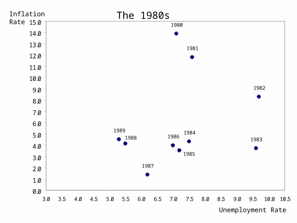
1980
1981
1982
19831984
1985
1986
1987
19881989
0.0
1.0
2.0
3.0
4.0
5.0
6.0
7.0
8.0
9.0
10.0
11.0
12.0
13.0
14.0
15.0
3.0 3.5 4.0 4.5 5.0 5.5 6.0 6.5 7.0 7.5 8.0 8.5 9.0 9.5 10.0 10.5
Unemployment Rate
Inflation Rate The 1980s
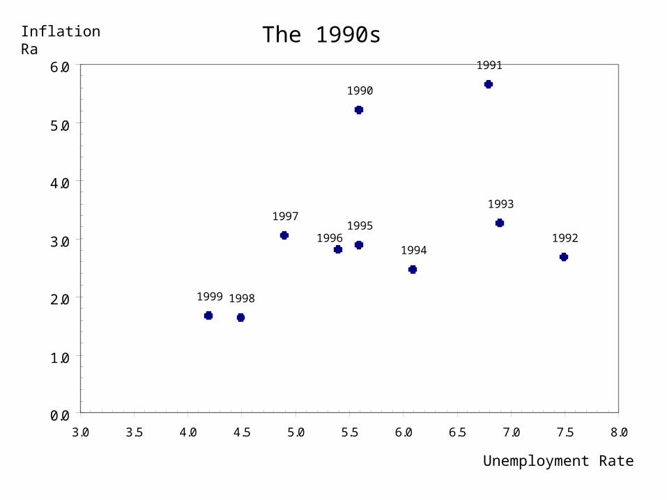
Unemployment Rate
Inflation Rate
1990
1991
1992
1993
1994
19951996
1997
19981999
0.0
1.0
2.0
3.0
4.0
5.0
6.0
3.0 3.5 4.0 4.5 5.0 5.5 6.0 6.5 7.0 7.5 8.0
The 1990s
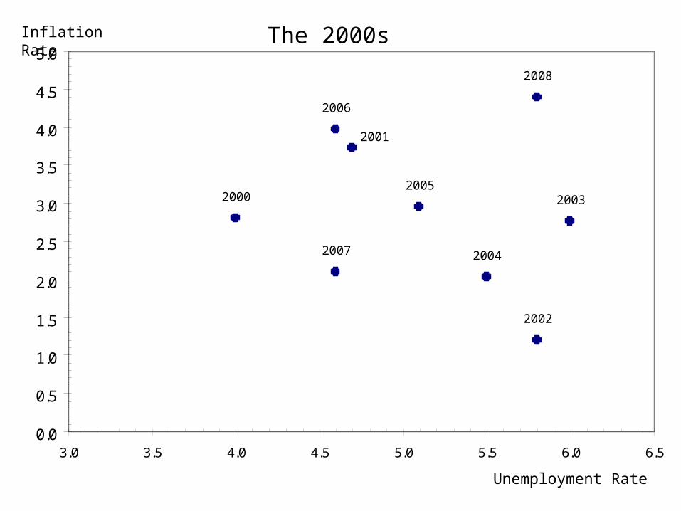
2000
2001
2002
2003
2004
2005
2006
2007
2008
0.0
0.5
1.0
1.5
2.0
2.5
3.0
3.5
4.0
4.5
5.0
3.0 3.5 4.0 4.5 5.0 5.5 6.0 6.5
Unemployment Rate
Inflation Rate The 2000s
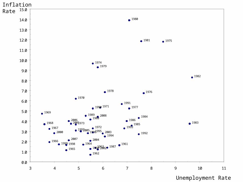
1968
19601961
1962
19631964
1965
1966
1967
1969
1970
1971
19721973
1974
1975
1976
1977
1978
1979
1980
1981
1982
1983
1984
1985
1986
1987
19881989
1990
1991
1992
1993
1994
199519961997
19981999
2000
2001
2002
2003
2004
2005
2006
2007
2008
0.0
1.0
2.0
3.0
4.0
5.0
6.0
7.0
8.0
9.0
10.0
11.0
12.0
13.0
14.0
15.0
3 4 5 6 7 8 9 10 11
Unemployment Rate
Inflation Rate
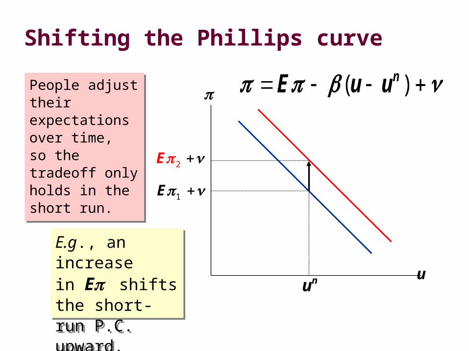
Shifting the Phillips curve
People adjust their expectations over time, so the tradeoff only holds in the short run.
People adjust their expectations over time, so the tradeoff only holds in the short run.
u
nu
1E
2E
E.g., an increase
in E shifts the short-run P.C. upward.
E.g., an increase
in E shifts the short-run P.C. upward.
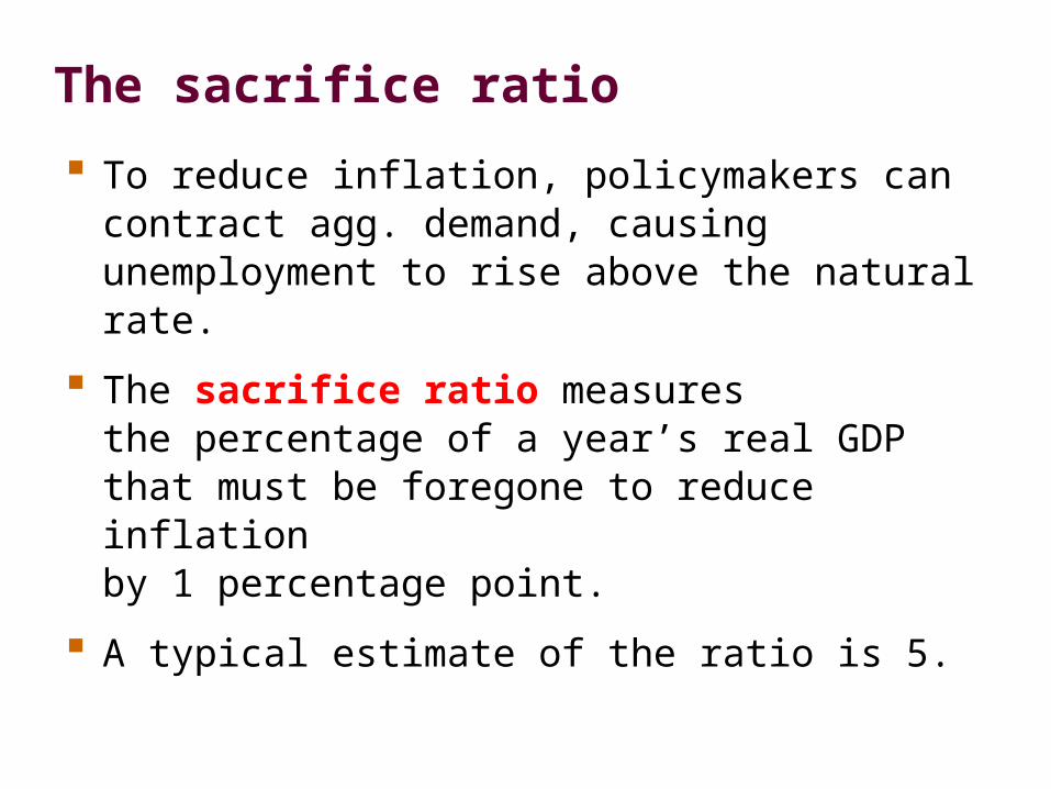
The sacrifice ratio
To reduce inflation, policymakers can contract agg. demand, causing unemployment to rise above the natural rate.
The sacrifice ratio measures the percentage of a year’s real GDP that must be foregone to reduce inflation by 1 percentage point.
A typical estimate of the ratio is 5.
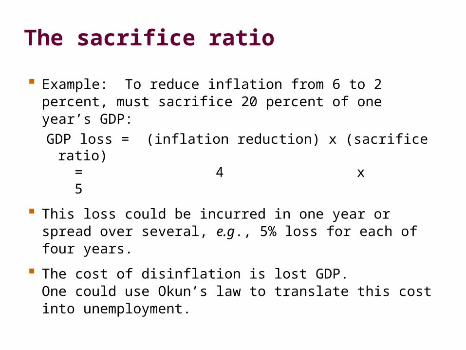
The sacrifice ratio
Example: To reduce inflation from 6 to 2 percent, must sacrifice 20 percent of one year’s GDP:
GDP loss = (inflation reduction) x (sacrifice ratio) = 4 x 5
This loss could be incurred in one year or spread over several, e.g., 5% loss for each of four years.
The cost of disinflation is lost GDP. One could use Okun’s law to translate this cost into unemployment.
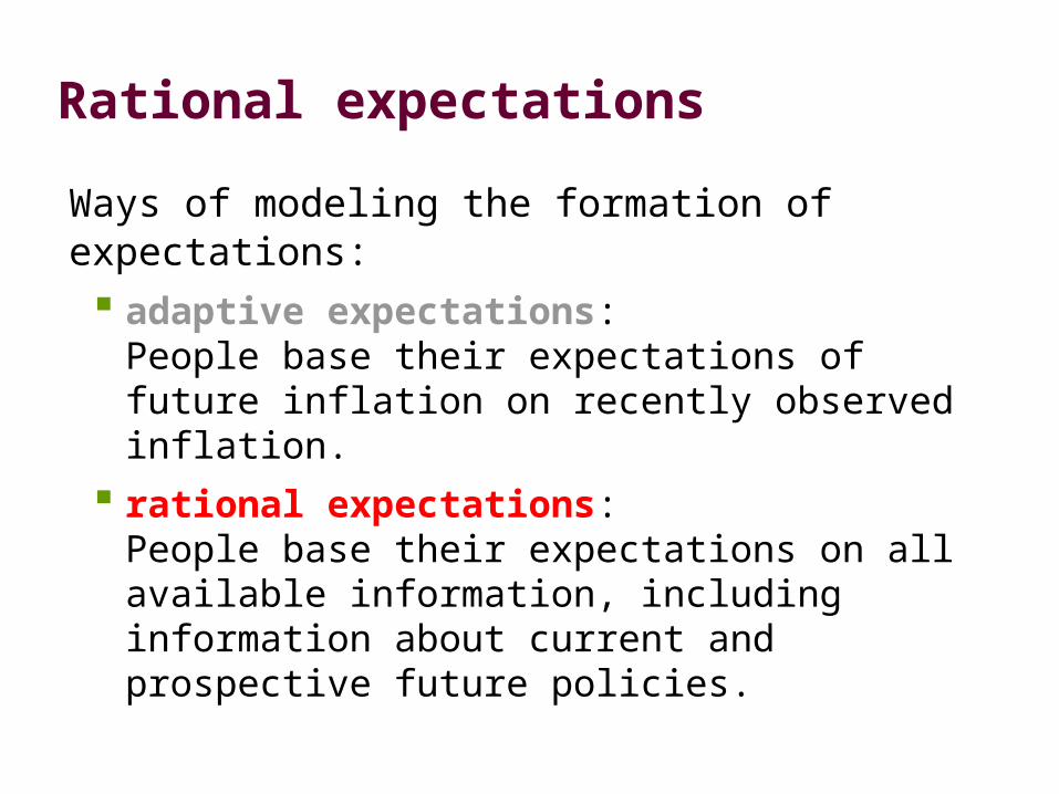
Rational expectations
Ways of modeling the formation of expectations:
adaptive expectations: People base their expectations of future inflation on recently observed inflation.
rational expectations:People base their expectations on all available information, including information about current and prospective future policies.
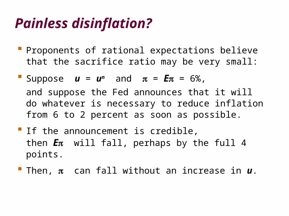
Painless disinflation?
Proponents of rational expectations believe that the sacrifice ratio may be very small:
Suppose u = un and = E = 6%,
and suppose the Fed announces that it will do whatever is necessary to reduce inflation from 6 to 2 percent as soon as possible.
If the announcement is credible, then E will fall, perhaps by the full 4 points.
Then, can fall without an increase in u.
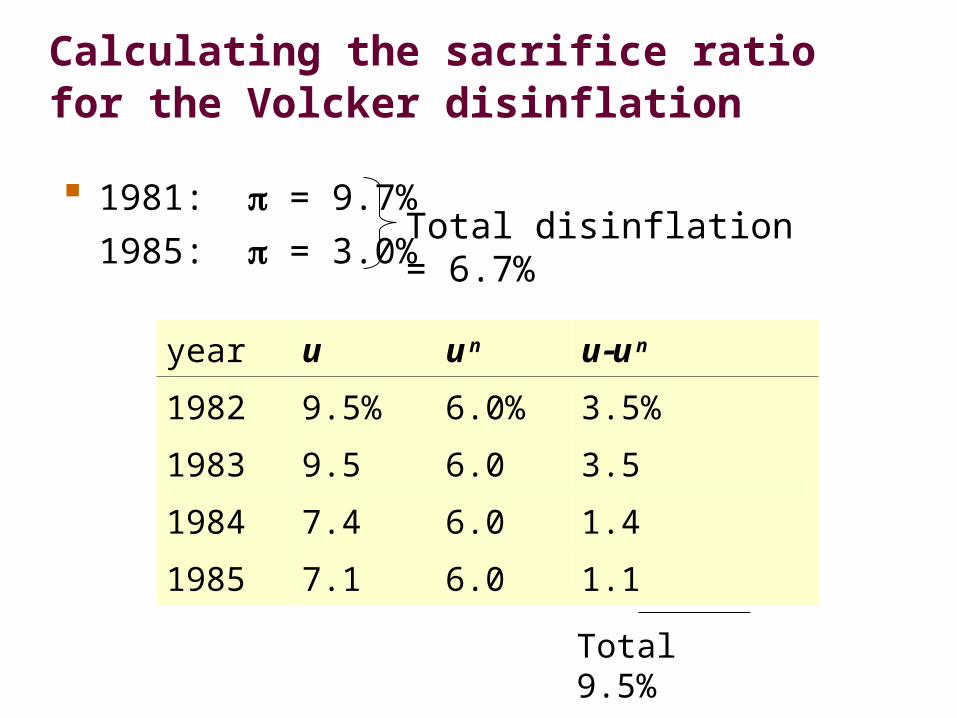
Calculating the sacrifice ratio for the Volcker disinflation
1981: = 9.7%
1985: = 3.0%
year u u n uu
n
1982 9.5% 6.0% 3.5%
1983 9.5 6.0 3.5
1984 7.4 6.0 1.4
1985 7.1 6.0 1.1
Total 9.5%
Total disinflation = 6.7%
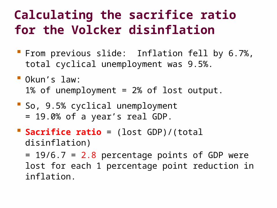
Calculating the sacrifice ratio for the Volcker disinflation
From previous slide: Inflation fell by 6.7%, total cyclical unemployment was 9.5%.
Okun’s law: 1% of unemployment = 2% of lost output.
So, 9.5% cyclical unemployment = 19.0% of a year’s real GDP.
Sacrifice ratio = (lost GDP)/(total disinflation)
= 19/6.7 = 2.8 percentage points of GDP were lost for each 1 percentage point reduction in inflation.
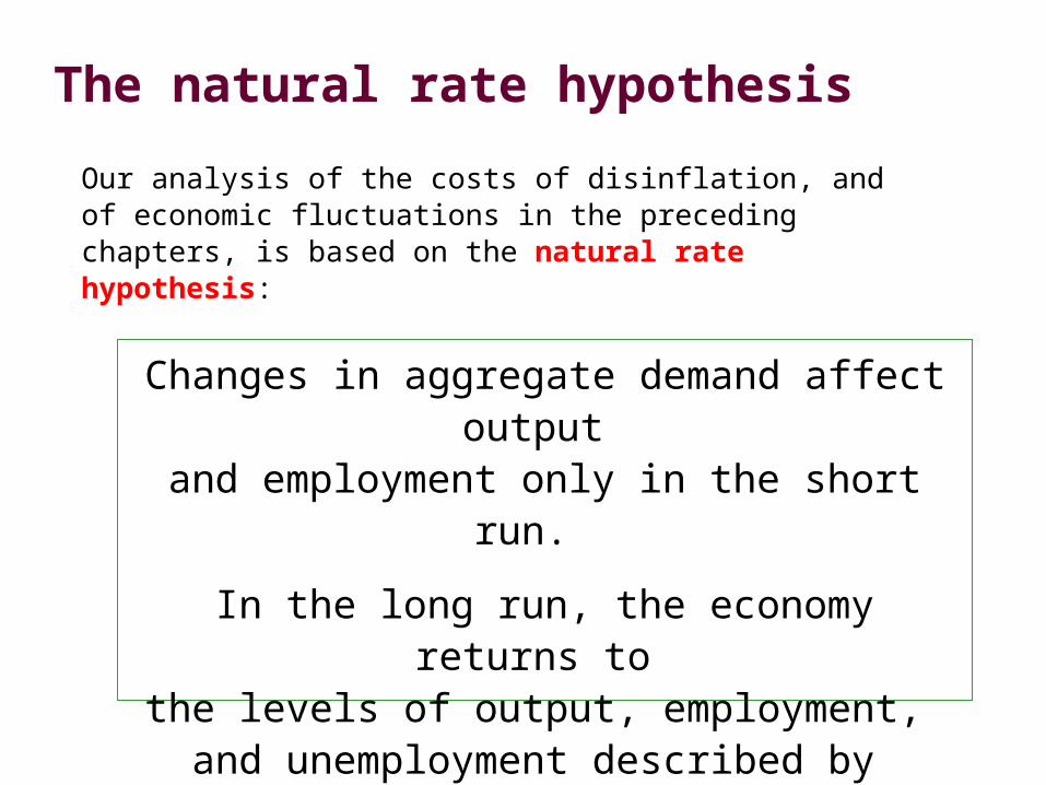
The natural rate hypothesis
Our analysis of the costs of disinflation, and of economic fluctuations in the preceding chapters, is based on the natural rate hypothesis:
Changes in aggregate demand affect output and employment only in the short run.
In the long run, the economy returns to the levels of output, employment, and unemployment described by the classical model (Chaps. 3-8).
Stabilization Policy
Should policy be active or passive?
Should policy be by rule or discretion?
Should policy be active or passive?
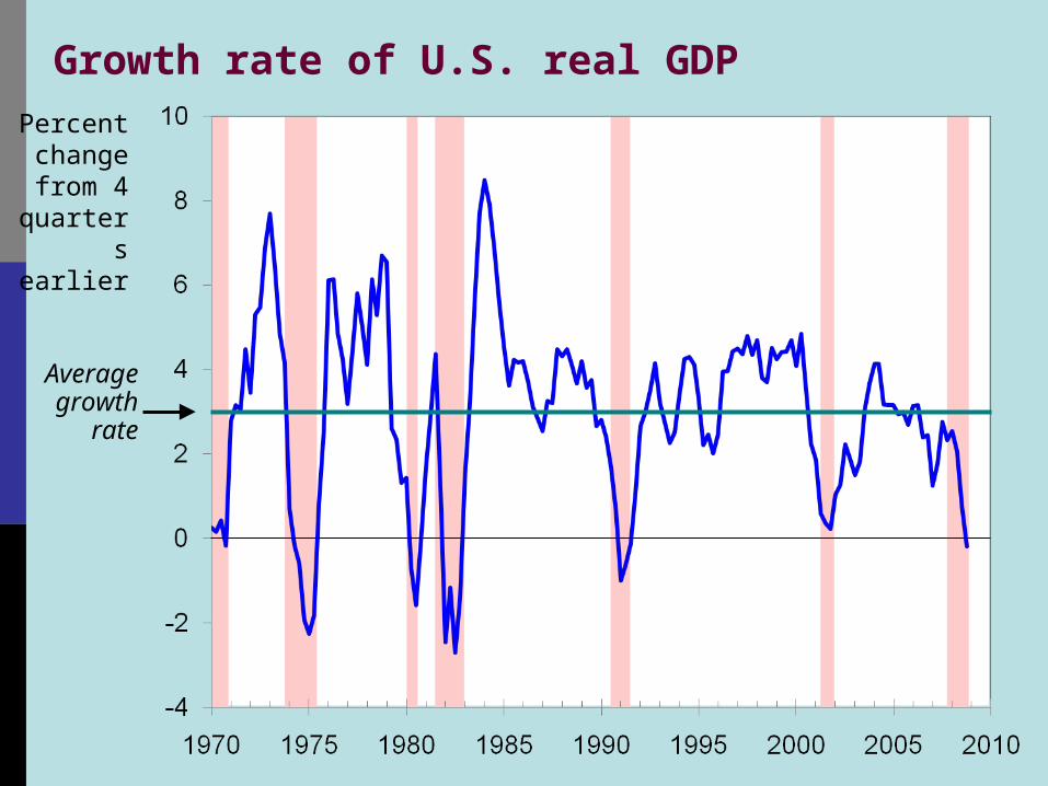
Growth rate of U.S. real GDPPercent change from 4
quarters earlier
Average growth
rate
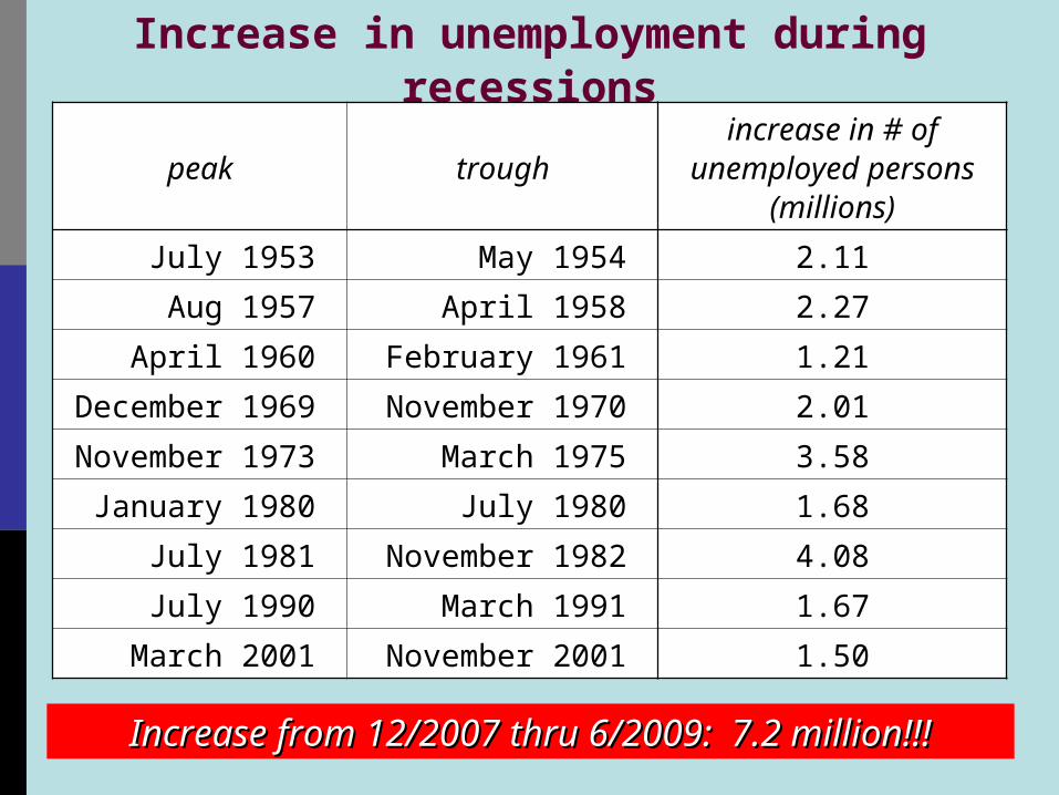
Increase in unemployment during recessions
peak troughincrease in # of
unemployed persons (millions)
July 1953 May 1954 2.11
Aug 1957 April 1958 2.27
April 1960 February 1961 1.21
December 1969 November 1970 2.01
November 1973 March 1975 3.58
January 1980 July 1980 1.68
July 1981 November 1982 4.08
July 1990 March 1991 1.67
March 2001 November 2001 1.50
Increase from 12/2007 thru 6/2009: 7.2 million!!!Increase from 12/2007 thru 6/2009: 7.2 million!!!
Arguments for active policy
Recessions cause economic hardship for millions of people.
The Employment Act of 1946: “It is the continuing policy and responsibility of the Federal Government to…promote full employment and production.”
The model of aggregate demand and supply (Chaps. 9-13) shows how fiscal and monetary policy can respond to shocks and stabilize the economy.
Arguments against active policy
Policies act with long & variable lags, including:inside lag: the time between the shock and the policy response.
takes time to recognize shock takes time to implement policy,
especially fiscal policy
outside lag: the time it takes for policy to affect economy.
If conditions change before policy’s impact is felt, the policy may destabilize the economy.
If conditions change before policy’s impact is felt, the policy may destabilize the economy.
Automatic stabilizers
definition: policies that stimulate or depress the economy when necessary without any deliberate policy change.
Designed to reduce the lags associated with stabilization policy.
Examples: income tax unemployment insurance welfare
Forecasting the macroeconomy
Because policies act with lags, policymakers must predict future conditions.
Two ways economists generate forecasts:Leading economic indicators
data series that fluctuate in advance of the economy
Macroeconometric models
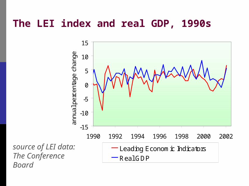
The LEI index and real GDP, 1990s
source of LEI data:The Conference Board
-15
-10
-5
0
5
10
15
1990 1992 1994 1996 1998 2000 2002
annu
al p
erce
ntag
e ch
ange
Leading Economic Indicators
Real GDP
Forecasting the macroeconomy
Because policies act with lags, policymakers must predict future conditions.
Two ways economists generate forecasts:Leading economic indicators
data series that fluctuate in advance of the economy
Macroeconometric modelsLarge-scale models with estimated parameters that can be used to forecast the response of endogenous variables to shocks and policies
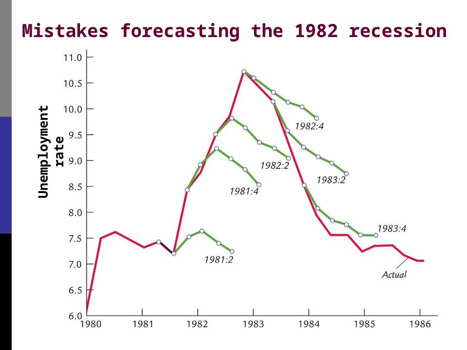
Mistakes forecasting the 1982 recessionU
ne
mp
loym
en
t ra
te
Forecasting the macroeconomy
Because policies act with lags, policymakers must predict future conditions.
The preceding slides show that the forecasts are often wrong.
This is one reason why some economists oppose policy activism.
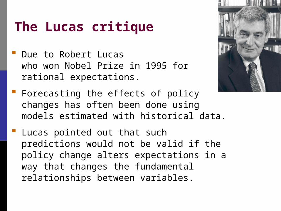
The Lucas critique
Due to Robert Lucaswho won Nobel Prize in 1995 for rational expectations.
Forecasting the effects of policy changes has often been done using models estimated with historical data.
Lucas pointed out that such predictions would not be valid if the policy change alters expectations in a way that changes the fundamental relationships between variables.
An example of the Lucas critique
Prediction (based on past experience):An increase in the money growth rate will reduce unemployment.
The Lucas critique points out that increasing the money growth rate may raise expected inflation, in which case unemployment would not necessarily fall.
The Jury’s out…
Looking at recent history does not clearly answer Question 1:
It’s hard to identify shocks in the data.
It’s hard to tell how outcomes would have been different had actual policies not been used.
The Great Moderation?
Question 2:
Should policy be conducted by Should policy be conducted by rule or discretion?rule or discretion?
Should policy be conducted by Should policy be conducted by rule or discretion?rule or discretion?
Rules and discretion: Basic concepts
Policy conducted by rule: Policymakers announce in advance how policy will respond in various situations, and commit themselves to following through.
Policy conducted by discretion:As events occur and circumstances change, policymakers use their judgment and apply whatever policies seem appropriate at the time.
Arguments for rules
1. Distrust of policymakers and the political process misinformed politicians politicians’ interests sometimes not the same
as the interests of society
Arguments for rules
2. The time inconsistency of discretionary policy def: A scenario in which policymakers
have an incentive to renege on a previously announced policy once others have acted on that announcement.
Destroys policymakers’ credibility, thereby reducing effectiveness of their policies.
Examples of time inconsistency
1. To encourage investment, govt announces it will not tax income from capital.
But once the factories are built, govt reneges in order to raise more tax revenue.
Examples of time inconsistency
2. To reduce expected inflation, the central bank announces it will tighten monetary policy.
But faced with high unemployment, the central bank may be tempted to cut interest rates.
Examples of time inconsistency
3. Aid is given to poor countries contingent on fiscal reforms.
The reforms do not occur, but aid is given anyway, because the donor countries do not want the poor countries’ citizens to starve.
Monetary policy rules
a. Constant money supply growth rate Advocated by monetarists. Stabilizes aggregate demand only if velocity
is stable.
Monetary policy rules
b. Target growth rate of nominal GDP Automatically increase money growth
whenever nominal GDP grows slower than targeted; decrease money growth when nominal GDP growth exceeds target.
a. Constant money supply growth rate
Monetary policy rules
c. Target the inflation rate Automatically reduce money growth whenever
inflation rises above the target rate. Many countries’ central banks now practice
inflation targeting, but allow themselves a little discretion.
a. Constant money supply growth rate
b. Target growth rate of nominal GDP
Central bank independence
A policy rule announced by central bank will work only if the announcement is credible.
Credibility depends in part on degree of independence of central bank.
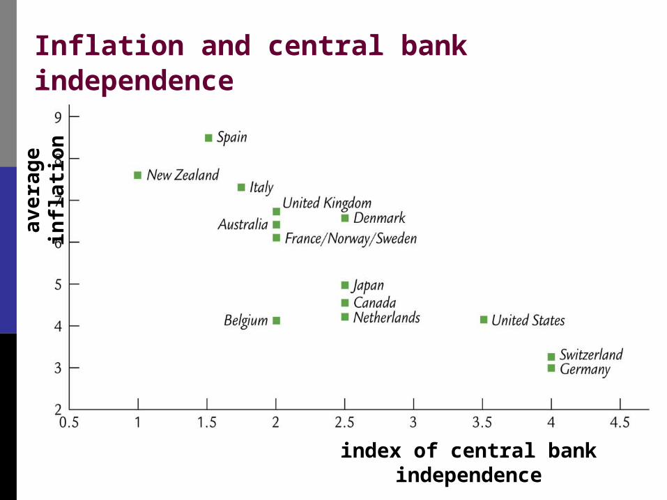
Inflation and central bank independence
aver
age
infl
atio
n
index of central bank independence
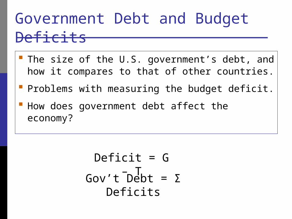
Government Debt and Budget Deficits The size of the U.S. government’s debt, and
how it compares to that of other countries.
Problems with measuring the budget deficit.
How does government debt affect the economy?
Deficit = G – T
Gov’t Debt = Σ Deficits
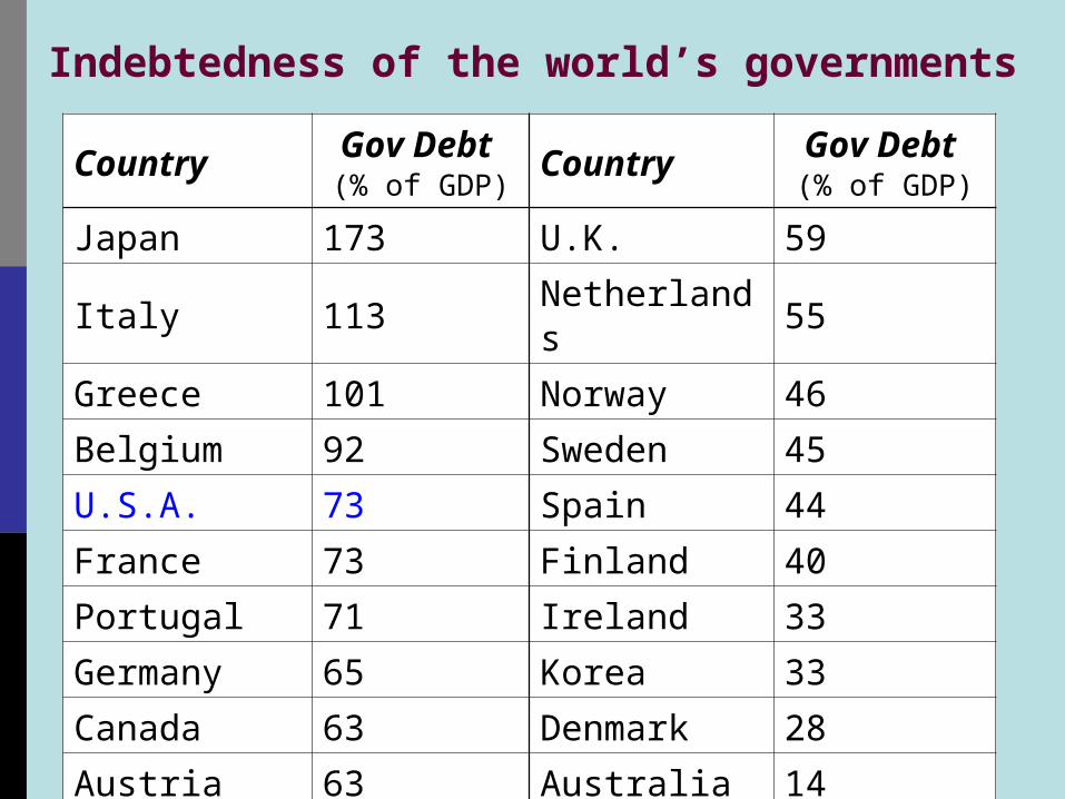
Indebtedness of the world’s governments
Country Gov Debt (% of GDP)
Country Gov Debt (% of GDP)
Japan 173 U.K. 59
Italy 113 Netherlands 55
Greece 101 Norway 46
Belgium 92 Sweden 45
U.S.A. 73 Spain 44
France 73 Finland 40
Portugal 71 Ireland 33
Germany 65 Korea 33
Canada 63 Denmark 28
Austria 63 Australia 14
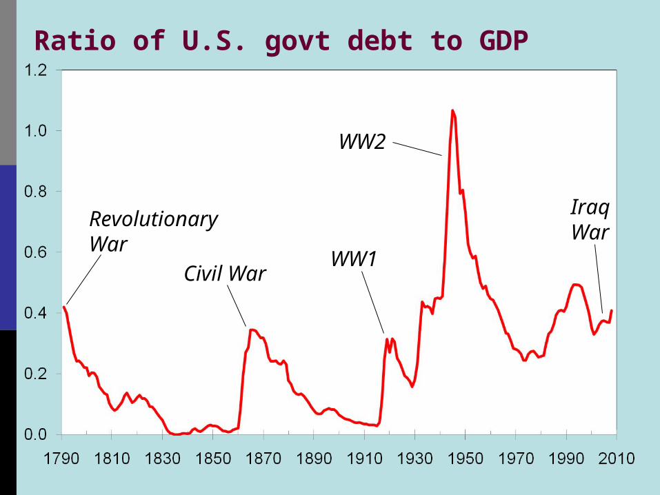
Ratio of U.S. govt debt to GDP
Revolutionary War
Civil WarWW1
WW2
Iraq War
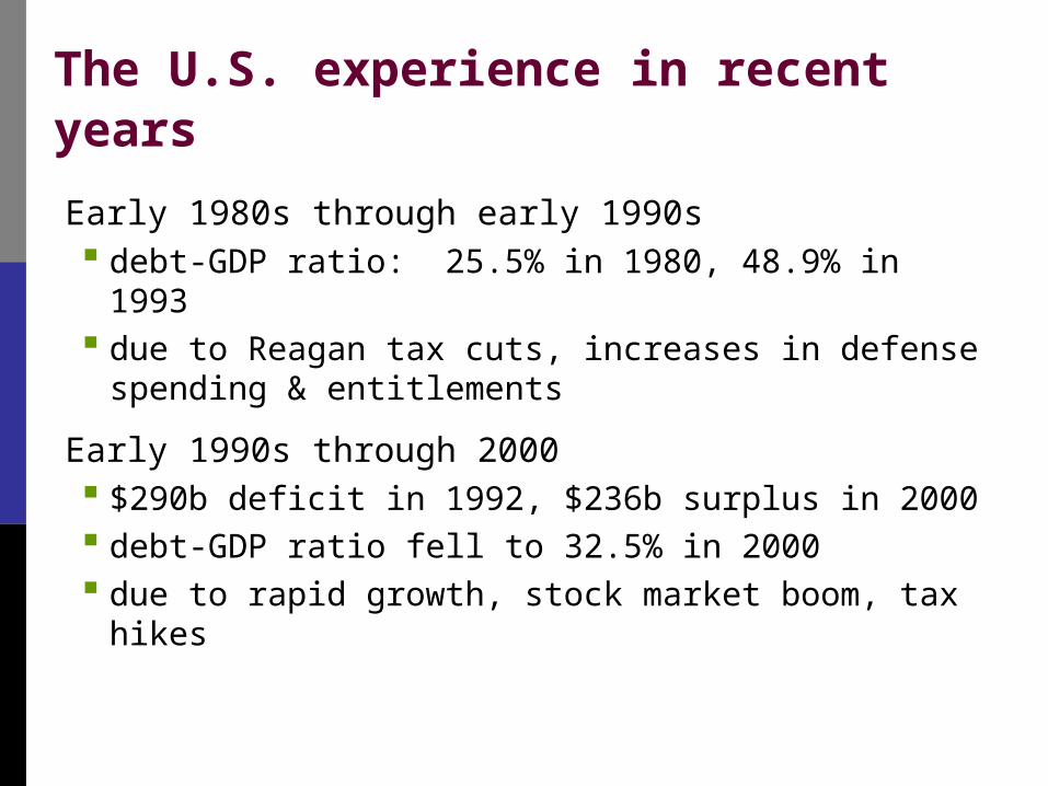
The U.S. experience in recent years
Early 1980s through early 1990s debt-GDP ratio: 25.5% in 1980, 48.9% in 1993 due to Reagan tax cuts, increases in defense
spending & entitlements
Early 1990s through 2000 $290b deficit in 1992, $236b surplus in 2000 debt-GDP ratio fell to 32.5% in 2000 due to rapid growth, stock market boom, tax
hikes
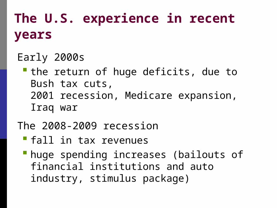
The U.S. experience in recent years
Early 2000s the return of huge deficits, due to Bush tax cuts,
2001 recession, Medicare expansion, Iraq war
The 2008-2009 recession fall in tax revenues huge spending increases (bailouts of financial
institutions and auto industry, stimulus package)
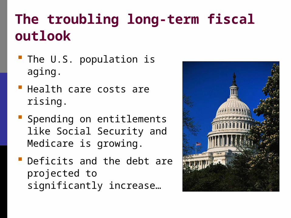
The troubling long-term fiscal outlook
The U.S. population is aging.
Health care costs are rising.
Spending on entitlements like Social Security and Medicare is growing.
Deficits and the debt are projected to significantly increase…
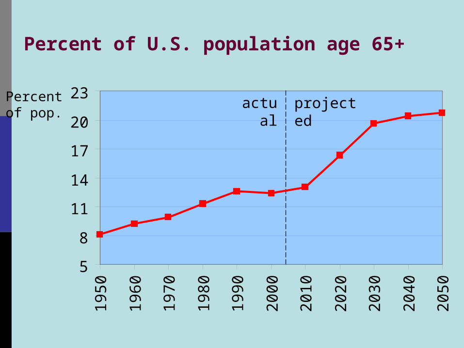
Percent of U.S. population age 65+
Percent of pop.
5
8
11
14
17
20
2319
50
1960
1970
1980
1990
2000
2010
2020
2030
2040
2050
actual projected
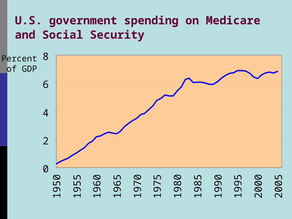
U.S. government spending on Medicare and Social Security
Percent of GDP
0
2
4
6
819
50
1955
1960
1965
1970
1975
1980
1985
1990
1995
2000
2005
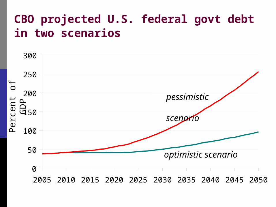
CBO projected U.S. federal govt debt in two scenarios
Pe
rce
nt o
f GD
P
0
50
100
150
200
250
300
2005 2010 2015 2020 2025 2030 2035 2040 2045 2050
optimistic scenario
pessimistic scenario
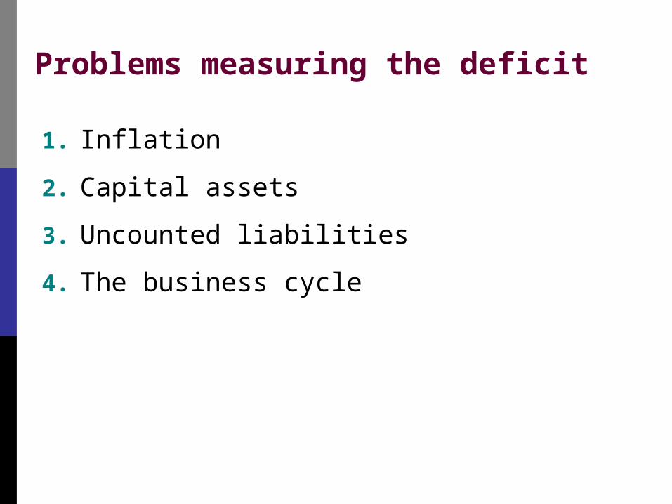
Problems measuring the deficit
1. Inflation
2. Capital assets
3. Uncounted liabilities
4. The business cycle
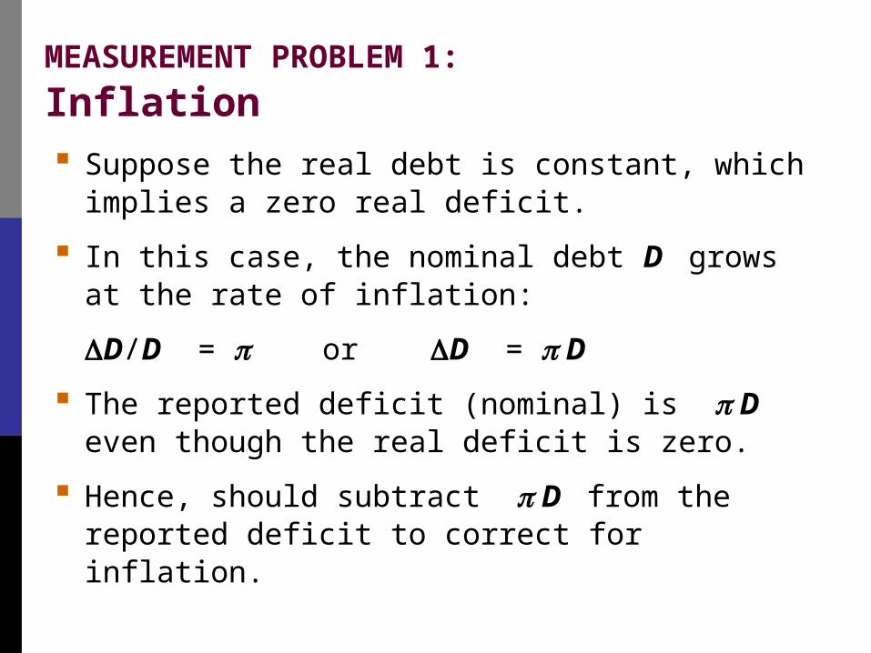
MEASUREMENT PROBLEM 1:
Inflation Suppose the real debt is constant, which implies a
zero real deficit.
In this case, the nominal debt D grows at the rate of inflation:
D/D = or D = D
The reported deficit (nominal) is D even though the real deficit is zero.
Hence, should subtract D from the reported deficit to correct for inflation.
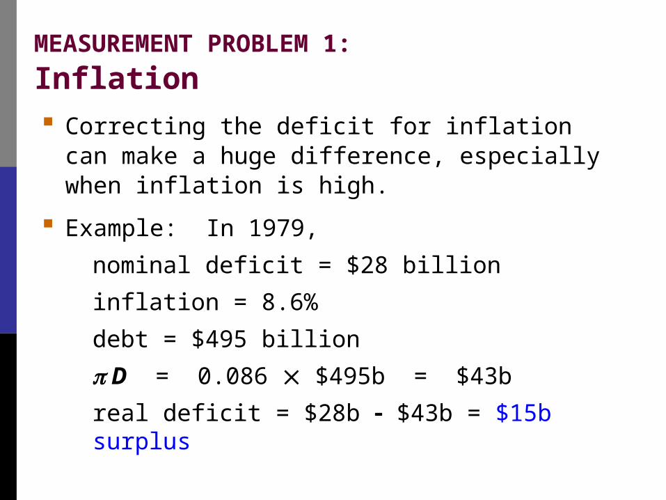
MEASUREMENT PROBLEM 1:
Inflation Correcting the deficit for inflation can make a huge
difference, especially when inflation is high.
Example: In 1979,
nominal deficit = $28 billion
inflation = 8.6%
debt = $495 billion
D = 0.086 $495b = $43b
real deficit = $28b $43b = $15b surplus
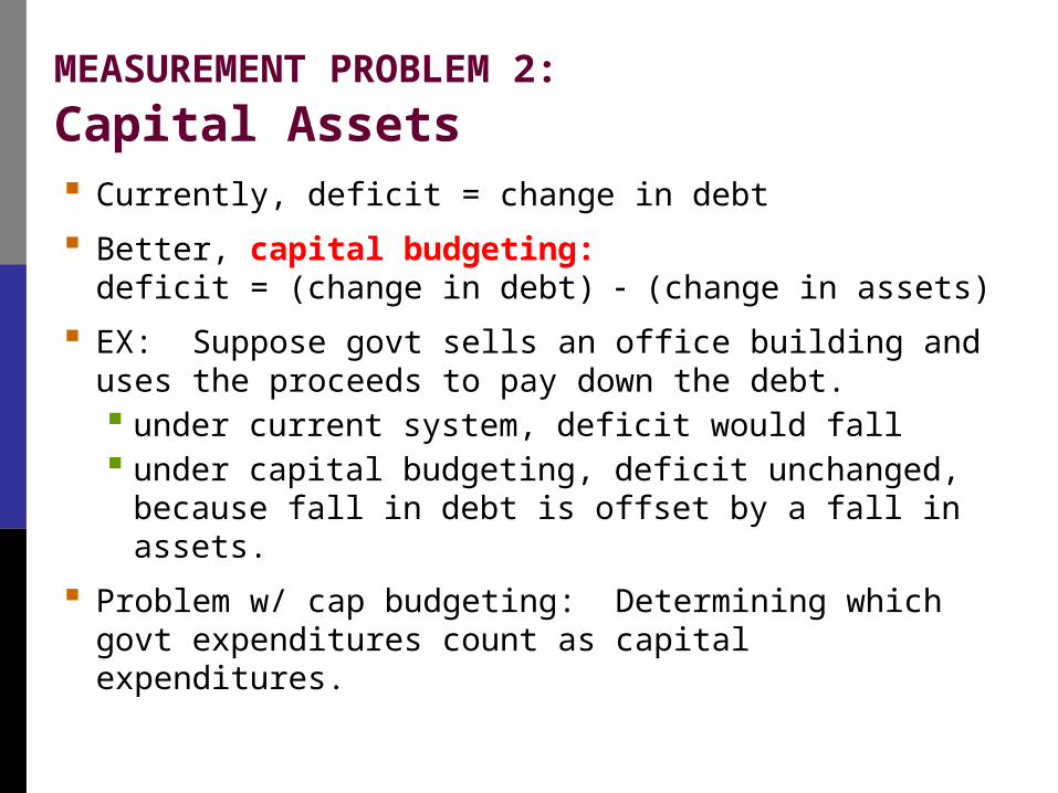
MEASUREMENT PROBLEM 2:
Capital Assets Currently, deficit = change in debt
Better, capital budgeting:deficit = (change in debt) (change in assets)
EX: Suppose govt sells an office building and uses the proceeds to pay down the debt. under current system, deficit would fall under capital budgeting, deficit unchanged,
because fall in debt is offset by a fall in assets.
Problem w/ cap budgeting: Determining which govt expenditures count as capital expenditures.
MEASUREMENT PROBLEM 3:
Uncounted liabilities
Current measure of deficit omits important liabilities of the government:
future pension payments owed to current govt workers
future Social Security payments
contingent liabilities, e.g., covering federally insured deposits when banks fail(Hard to attach a dollar value to contingent liabilities, due to inherent uncertainty.)
MEASUREMENT PROBLEM 4:
The business cycle
The deficit varies over the business cycle due to automatic stabilizers (unemployment insurance, the income tax system).
These are not measurement errors, but do make it harder to judge fiscal policy stance. E.g., is an observed increase in deficit
due to a downturn or an expansionary shift in fiscal policy?
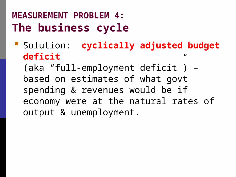
MEASUREMENT PROBLEM 4:
The business cycle
Solution: cyclically adjusted budget deficit (aka “full-employment deficit”) – based on estimates of what govt spending & revenues would be if economy were at the natural rates of output & unemployment.
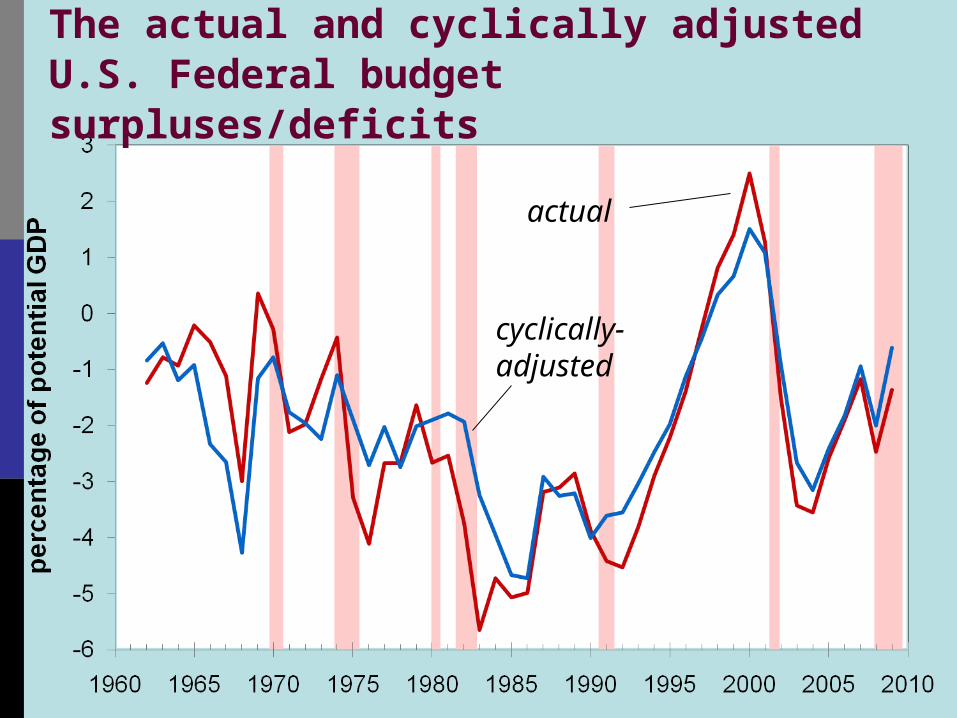
The actual and cyclically adjusted U.S. Federal budget surpluses/deficits
actual
cyclically-adjusted
The bottom line
We must exercise care We must exercise care
when interpreting when interpreting
the reported deficit figures.the reported deficit figures.
We must exercise care We must exercise care
when interpreting when interpreting
the reported deficit figures.the reported deficit figures.
Is the govt debt really a problem?Consider a tax cut with corresponding increase in the government debt.
Two viewpoints:
1. Traditional view
2. Ricardian view
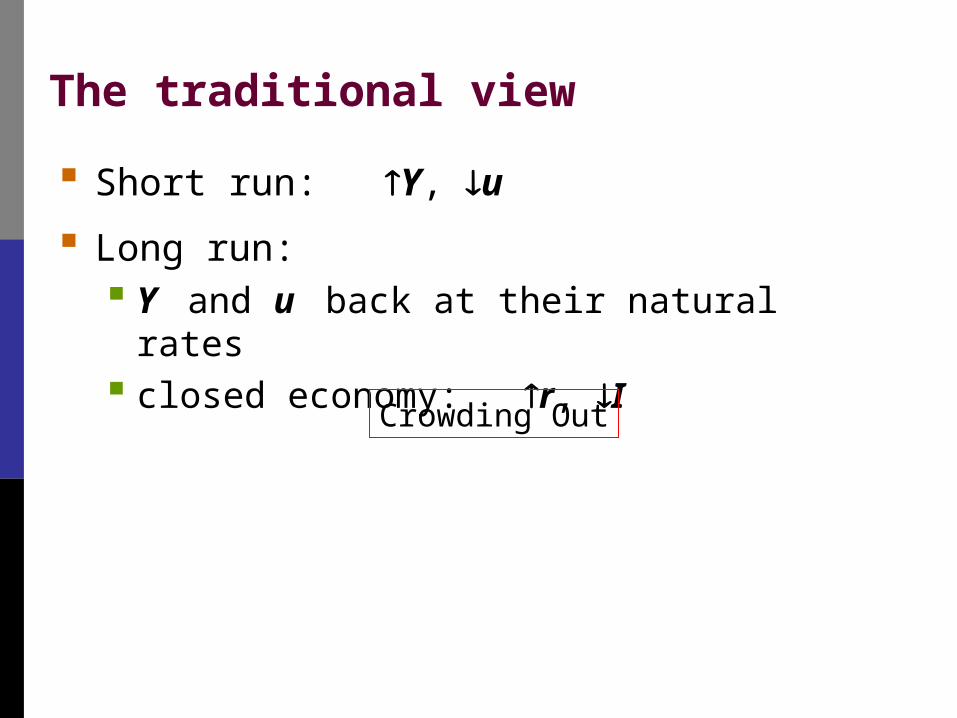
The traditional view
Short run: Y, u
Long run: Y and u back at their natural rates closed economy: r, I
Crowding Out
The Ricardian view
due to David Ricardo (1820), more recently advanced by Robert Barro
According to Ricardian equivalence, a debt-financed tax cut has no effect on consumption, national saving, the real interest rate, investment, net exports, or real GDP, even in the short run.
The logic of Ricardian Equivalence
Consumers are forward-looking, know that a debt-financed tax cut today implies an increase in future taxes that is equal – in present value – to the tax cut.
The tax cut does not make consumers better off, so they do not increase consumption spending.
Instead, they save the full tax cut in order to repay the future tax liability.
Result: Private saving rises by the amount public saving falls, leaving national saving unchanged.
Problems with Ricardian Equivalence
Myopia: Not all consumers think so far ahead, some see the tax cut as a windfall.
Borrowing constraints: Some consumers cannot borrow enough to achieve their optimal consumption, so they spend a tax cut.
Future generations: If consumers expect that the burden of repaying a tax cut will fall on future generations, then a tax cut now makes them feel better off, so they increase spending.
Evidence against Ricardian Equivalence?
Early 1980s: Reagan tax cuts increased deficit. National saving fell, real interest rate rose
1992:Income tax withholding reduced to stimulate economy. This delayed taxes but didn’t make consumers
better off. Almost half of consumers increased consumption.
Evidence against Ricardian Equivalence?
Proponents of R.E. argue that the Reagan tax cuts did not provide a fair test of R.E. Consumers may have expected the debt to be
repaid with future spending cuts instead of future tax hikes.
Private saving may have fallen for reasons other than the tax cut, such as optimism about the economy.
Because the data is subject to different interpretations, both views of govt debt survive.
OTHER PERSPECTIVES: Balanced budgets vs. optimal fiscal policy
Some politicians have proposed amending the U.S. Constitution to require balanced federal govt budget every year.
Many economists reject this proposal, arguing that deficit should be used to: stabilize output & employment smooth taxes in the face of fluctuating income redistribute income across generations when
appropriate
OTHER PERSPECTIVES:
Debt and politics“Fiscal policy is not made by angels…”
– Greg Mankiw, p.487
Some do not trust policymakers with deficit spending. They argue that:policymakers do not worry about true costs of their
spending, since burden falls on future taxpayers since future taxpayers cannot participate in the
decision process, their interests may not be taken into account
This is another reason for the proposals for a balanced budget amendment
OTHER PERSPECTIVES: Fiscal effects on monetary policy
Govt deficits may be financed by printing money A high govt debt may be an incentive for
policymakers to create inflation (to reduce real value of debt at expense of bond holders)

Clicker Questions
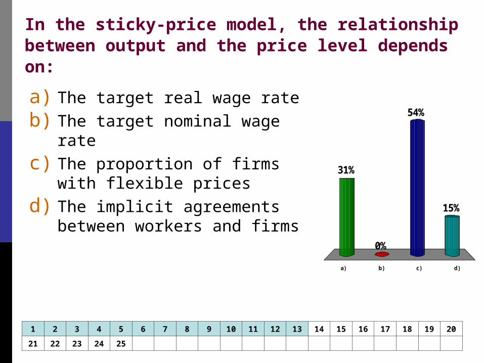
a) The target real wage rate
b) The target nominal wage rate
c) The proportion of firms with flexible prices
d) The implicit agreements between workers and firms
In the sticky-price model, the relationship between output and the price level depends on:
a) b) c) d)
31%
15%
54%
0%
1 2 3 4 5 6 7 8 9 10 11 12 13 14 15 16 17 18 19 20
21 22 23 24 25
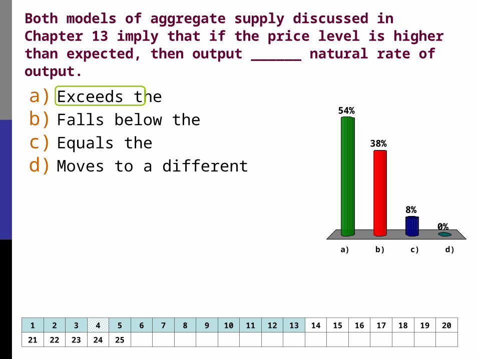
Both models of aggregate supply discussed in Chapter 13 imply that if the price level is higher than expected, then output ______ natural rate of output.
a) b) c) d)
54%
0%
8%
38%
a) Exceeds the
b) Falls below the
c) Equals the
d) Moves to a different
1 2 3 4 5 6 7 8 9 10 11 12 13 14 15 16 17 18 19 20
21 22 23 24 25
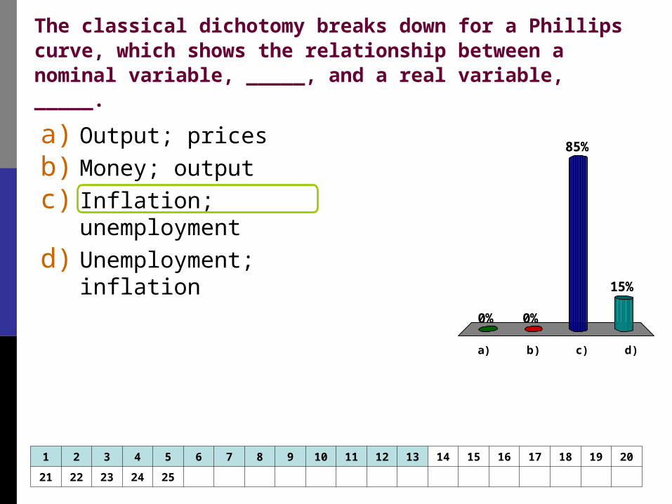
The classical dichotomy breaks down for a Phillips curve, which shows the relationship between a nominal variable, _____, and a real variable, _____.
a) b) c) d)
0%
15%
85%
0%
a) Output; prices
b) Money; output
c) Inflation; unemployment
d) Unemployment; inflation
1 2 3 4 5 6 7 8 9 10 11 12 13 14 15 16 17 18 19 20
21 22 23 24 25
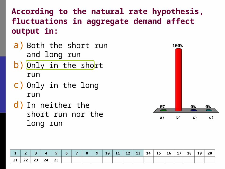
According to the natural rate hypothesis, fluctuations in aggregate demand affect output in:
a) b) c) d)
0% 0%0%
100%a) Both the short run and long run
b) Only in the short run
c) Only in the long run
d) In neither the short run nor the long run
1 2 3 4 5 6 7 8 9 10 11 12 13 14 15 16 17 18 19 20
21 22 23 24 25
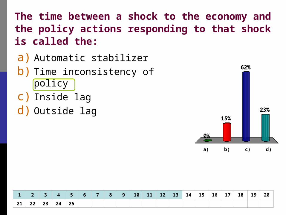
The time between a shock to the economy and the policy actions responding to that shock is called the:
a) b) c) d)
0%
23%
62%
15%
a) Automatic stabilizer
b) Time inconsistency of policy
c) Inside lag
d) Outside lag
1 2 3 4 5 6 7 8 9 10 11 12 13 14 15 16 17 18 19 20
21 22 23 24 25
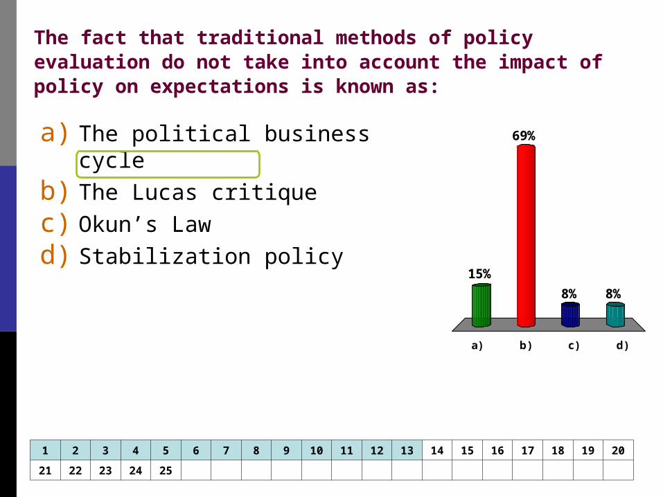
The fact that traditional methods of policy evaluation do not take into account the impact of policy on expectations is known as:
a) b) c) d)
15%
8%8%
69%a) The political business cycle
b) The Lucas critique
c) Okun’s Law
d) Stabilization policy
1 2 3 4 5 6 7 8 9 10 11 12 13 14 15 16 17 18 19 20
21 22 23 24 25
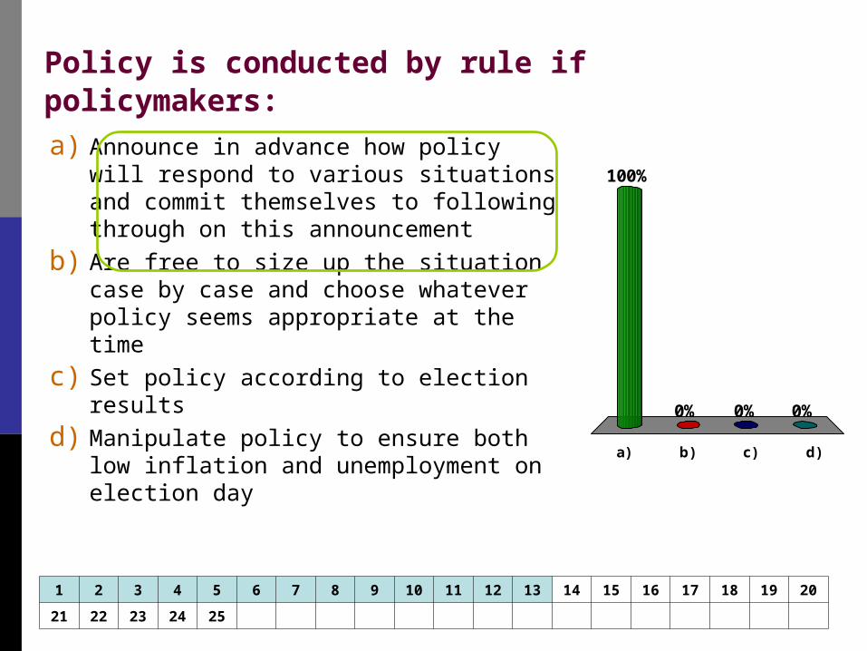
Policy is conducted by rule if policymakers:
a) b) c) d)
100%
0%0%0%
a) Announce in advance how policy will respond to various situations and commit themselves to following through on this announcement
b) Are free to size up the situation case by case and choose whatever policy seems appropriate at the time
c) Set policy according to election results
d) Manipulate policy to ensure both low inflation and unemployment on election day
1 2 3 4 5 6 7 8 9 10 11 12 13 14 15 16 17 18 19 20
21 22 23 24 25
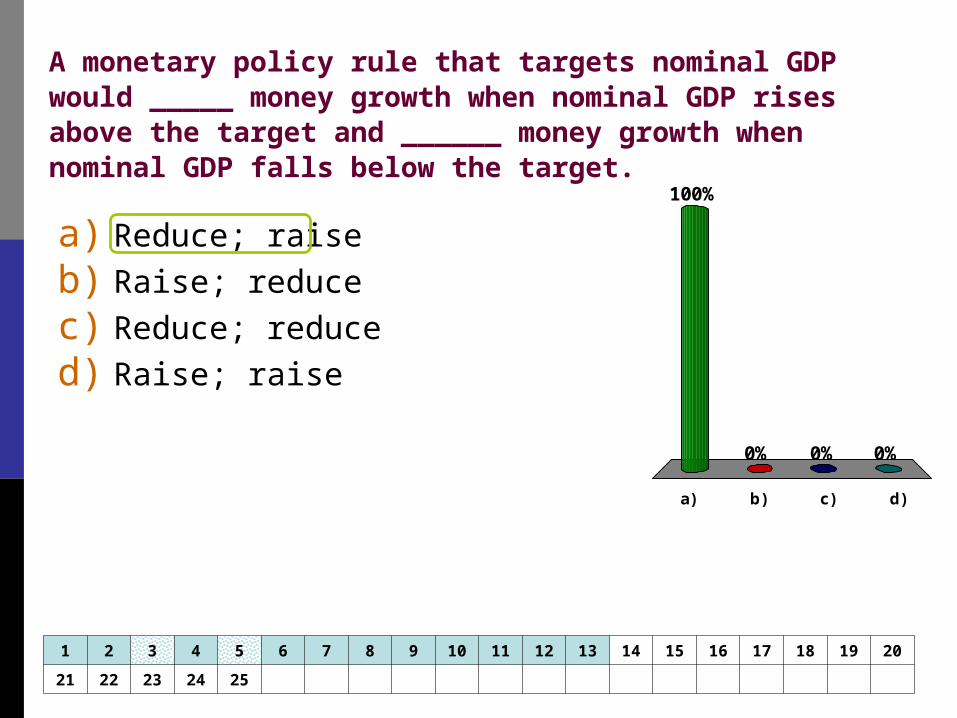
A monetary policy rule that targets nominal GDP would _____ money growth when nominal GDP rises above the target and ______ money growth when nominal GDP falls below the target.
a) b) c) d)
100%
0%0%0%
a) Reduce; raise
b) Raise; reduce
c) Reduce; reduce
d) Raise; raise
1 2 3 4 5 6 7 8 9 10 11 12 13 14 15 16 17 18 19 20
21 22 23 24 25
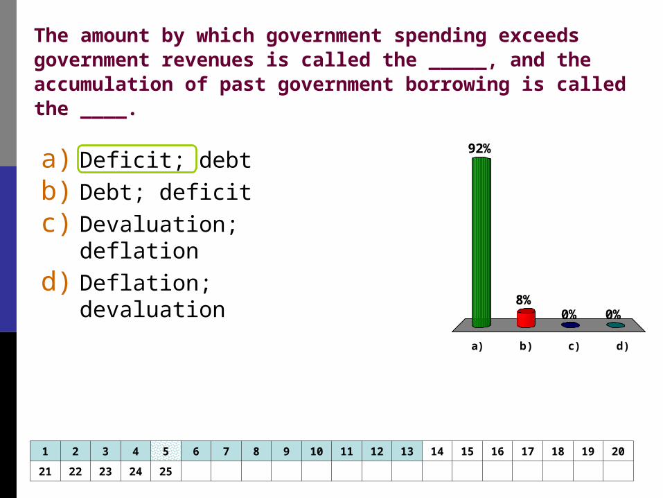
The amount by which government spending exceeds government revenues is called the _____, and the accumulation of past government borrowing is called the ____.
a) b) c) d)
92%
0%0%8%
a) Deficit; debt
b) Debt; deficit
c) Devaluation; deflation
d) Deflation; devaluation
1 2 3 4 5 6 7 8 9 10 11 12 13 14 15 16 17 18 19 20
21 22 23 24 25
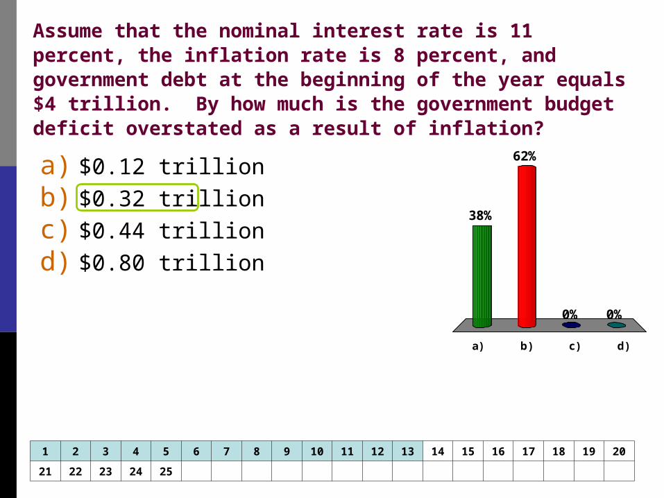
Assume that the nominal interest rate is 11 percent, the inflation rate is 8 percent, and government debt at the beginning of the year equals $4 trillion. By how much is the government budget deficit overstated as a result of inflation?
a) b) c) d)
38%
0%0%
62%a) $0.12 trillion
b) $0.32 trillion
c) $0.44 trillion
d) $0.80 trillion
1 2 3 4 5 6 7 8 9 10 11 12 13 14 15 16 17 18 19 20
21 22 23 24 25
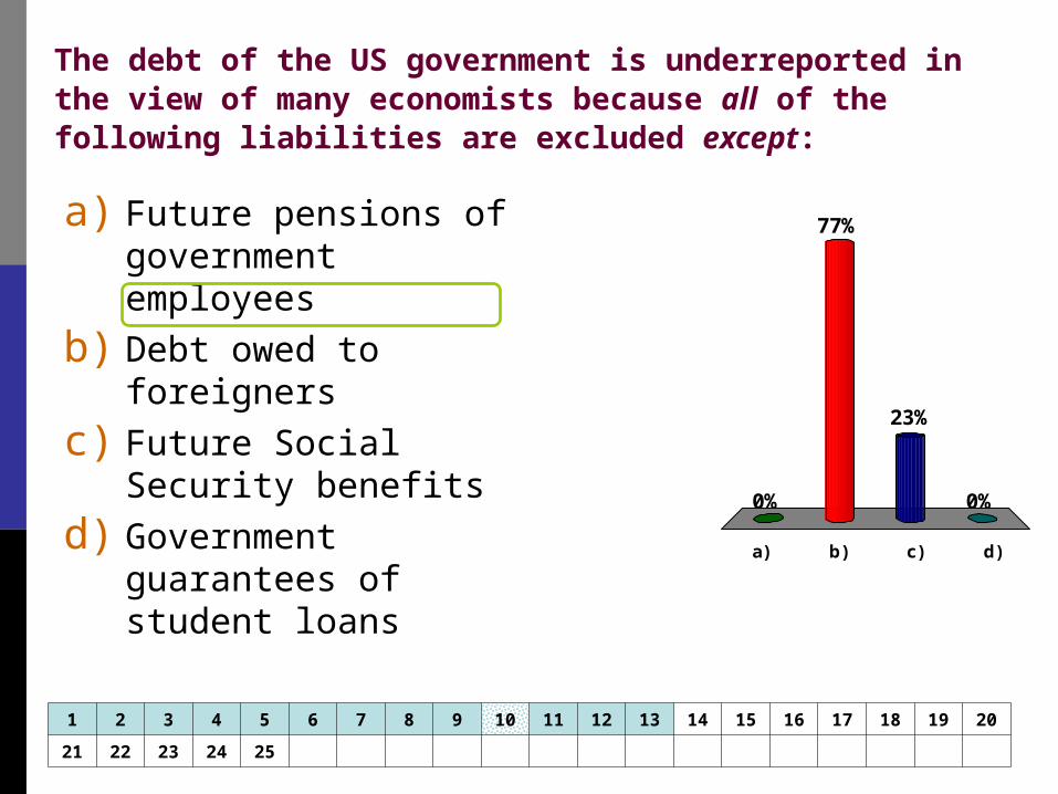
The debt of the US government is underreported in the view of many economists because all of the following liabilities are excluded except:
a) b) c) d)
0% 0%
23%
77%a) Future pensions of government employees
b) Debt owed to foreigners
c) Future Social Security benefits
d) Government guarantees of student loans
1 2 3 4 5 6 7 8 9 10 11 12 13 14 15 16 17 18 19 20
21 22 23 24 25
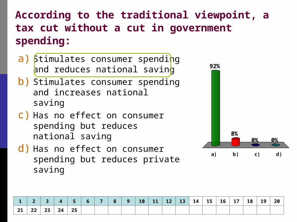
According to the traditional viewpoint, a tax cut without a cut in government spending:
a) b) c) d)
92%
0%0%8%
a) Stimulates consumer spending and reduces national saving
b) Stimulates consumer spending and increases national saving
c) Has no effect on consumer spending but reduces national saving
d) Has no effect on consumer spending but reduces private saving
1 2 3 4 5 6 7 8 9 10 11 12 13 14 15 16 17 18 19 20
21 22 23 24 25
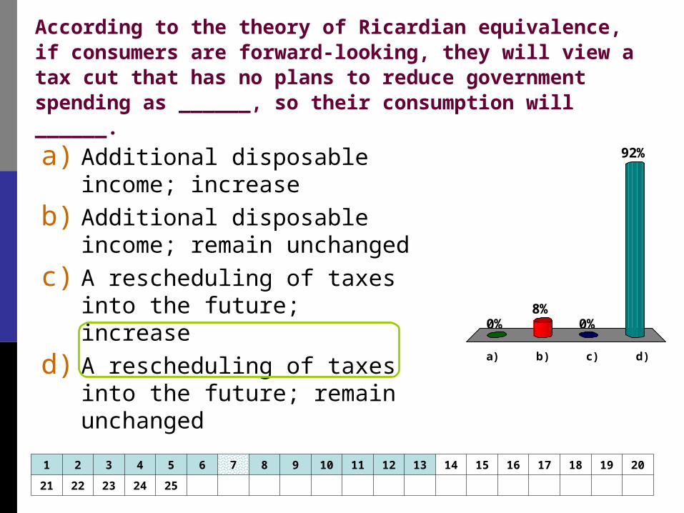
According to the theory of Ricardian equivalence, if consumers are forward-looking, they will view a tax cut that has no plans to reduce government spending as ______, so their consumption will ______.
a) b) c) d)
0%
92%
0%8%
a) Additional disposable income; increase
b) Additional disposable income; remain unchanged
c) A rescheduling of taxes into the future; increase
d) A rescheduling of taxes into the future; remain unchanged
1 2 3 4 5 6 7 8 9 10 11 12 13 14 15 16 17 18 19 20
21 22 23 24 25