Embed Size (px)
DESCRIPTION
nsit
Citation preview
ANALOG
&
DIGITAL
COMMUNICATION
LAB
FILE
NSIT SUBMITTED BY:-
NAME:-JAIDEEP KUMAR
ROLL NO :- 738/IT/13
INDEXS.NO. TOPIC DATE T.SIGN
EXPERIMENT NO.1
AIM-(a.) MATRIX COMPUTATION.
SOLUTION-
a=[1 6 3; 2 5 6; 3 6 8] b=[1 2 3; 4 5 6; 7 8 9]
OUTPUT OUTPUT
a = b=
1 6 3 1 2 3
2 5 6 4 5 6
3 6 8 7 8 9
r=a+2 c=a'
OUTPUT OUTPUT
r = 3 8 5 c = 1 2 3
4 7 8 6 5 6
5 8 10 3 6 8
d=a*b e=a.*b
OUTPUT OUTPUT
d = 46 56 66 e= 1 12 9
64 77 90 8 25 36
83 100 117 21 48 72
g=inv(a) d=det(a)
OUTPUT OUTPUT
g = d =
0.5714 -4.2857 3.0000 7
0.2857 -0.1429 0
-0.4286 1.7143 -1.0000
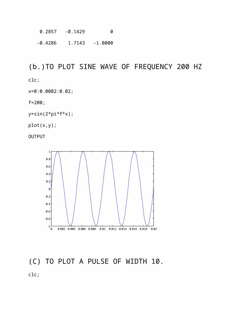
(b.)TO PLOT SINE WAVE OF FREQUENCY 200 HZ
clc;
x=0:0.0002:0.02;
f=200;
y=sin(2*pi*f*x);
plot(x,y);
OUTPUT
0 0.002 0.004 0.006 0.008 0.01 0.012 0.014 0.016 0.018 0.02
-1
-0.8
-0.6
-0.4
-0.2
0
0.2
0.4
0.6
0.8
1
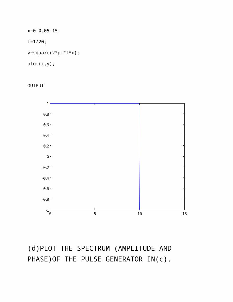
(C) TO PLOT A PULSE OF WIDTH 10.
clc;
x=0:0.05:15;
f=1/20;
y=square(2*pi*f*x);
plot(x,y);
OUTPUT
0 5 10 15-1
-0.8
-0.6
-0.4
-0.2
0
0.2
0.4
0.6
0.8
1
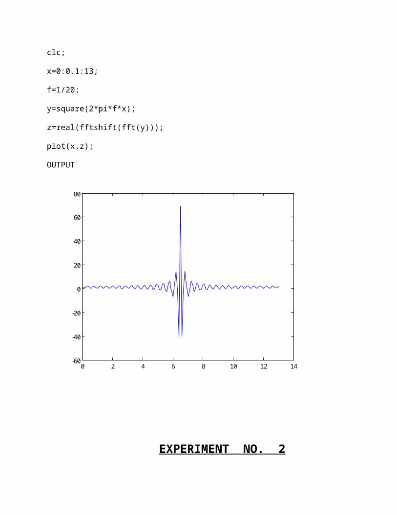
(d)PLOT THE SPECTRUM (AMPLITUDE AND PHASE)OF THE PULSE GENERATOR IN(c).
clc;
x=0:0.1:13;
f=1/20;
y=square(2*pi*f*x);
z=real(fftshift(fft(y)));
plot(x,z);
OUTPUT
0 2 4 6 8 10 12 14-60
-40
-20
0
20
40
60
80
EXPERIMENT NO. 2
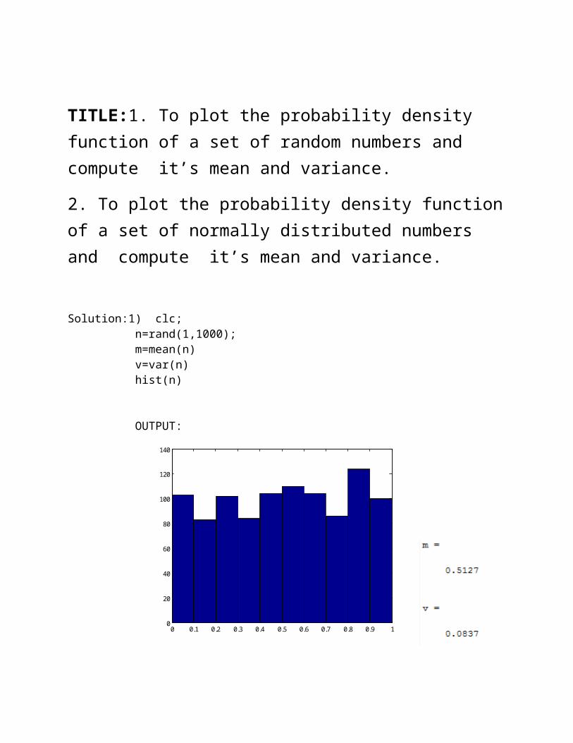
TITLE:1. To plot the probability density function of a set of random numbers and compute it’s mean and variance.
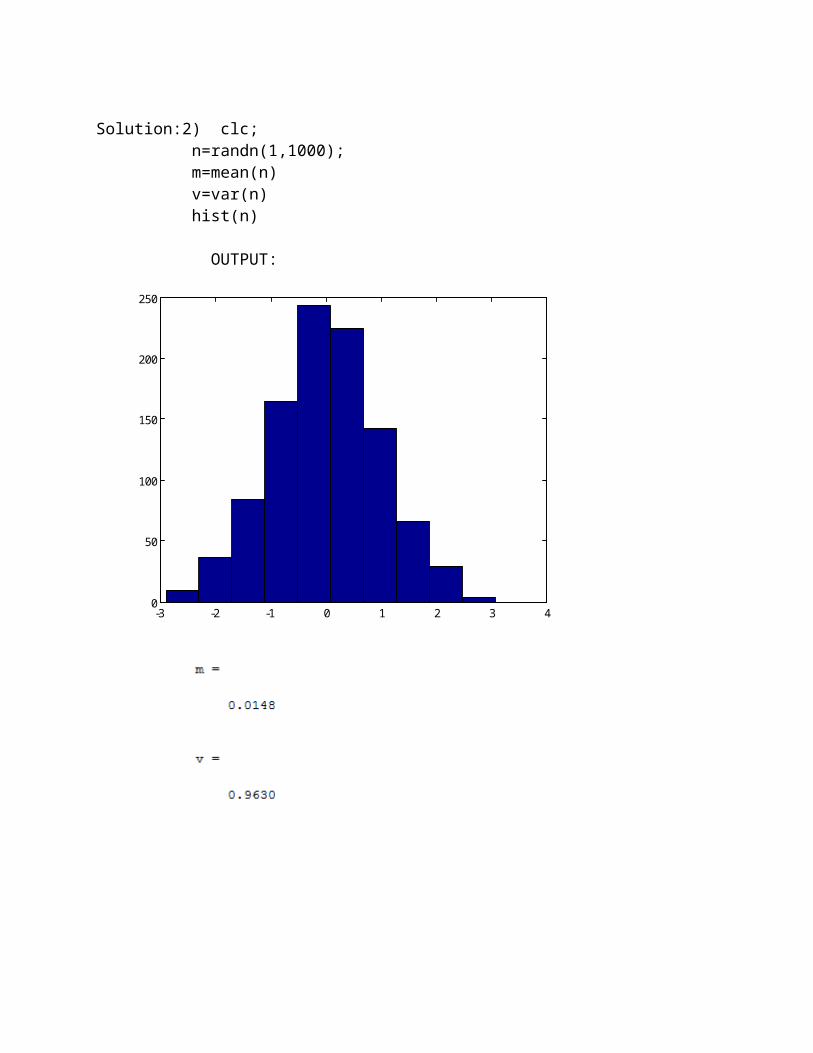
2. To plot the probability density function of a set of normally distributed numbers and compute it’s mean and variance.
Solution:1) clc;n=rand(1,1000);m=mean(n)v=var(n)hist(n)
OUTPUT:
0 0.1 0.2 0.3 0.4 0.5 0.6 0.7 0.8 0.9 10
20
40
60
80
100
120
140
Solution:2) clc;n=randn(1,1000);m=mean(n)v=var(n)hist(n)
OUTPUT:
-3 -2 -1 0 1 2 3 40
50
100
150
200
250
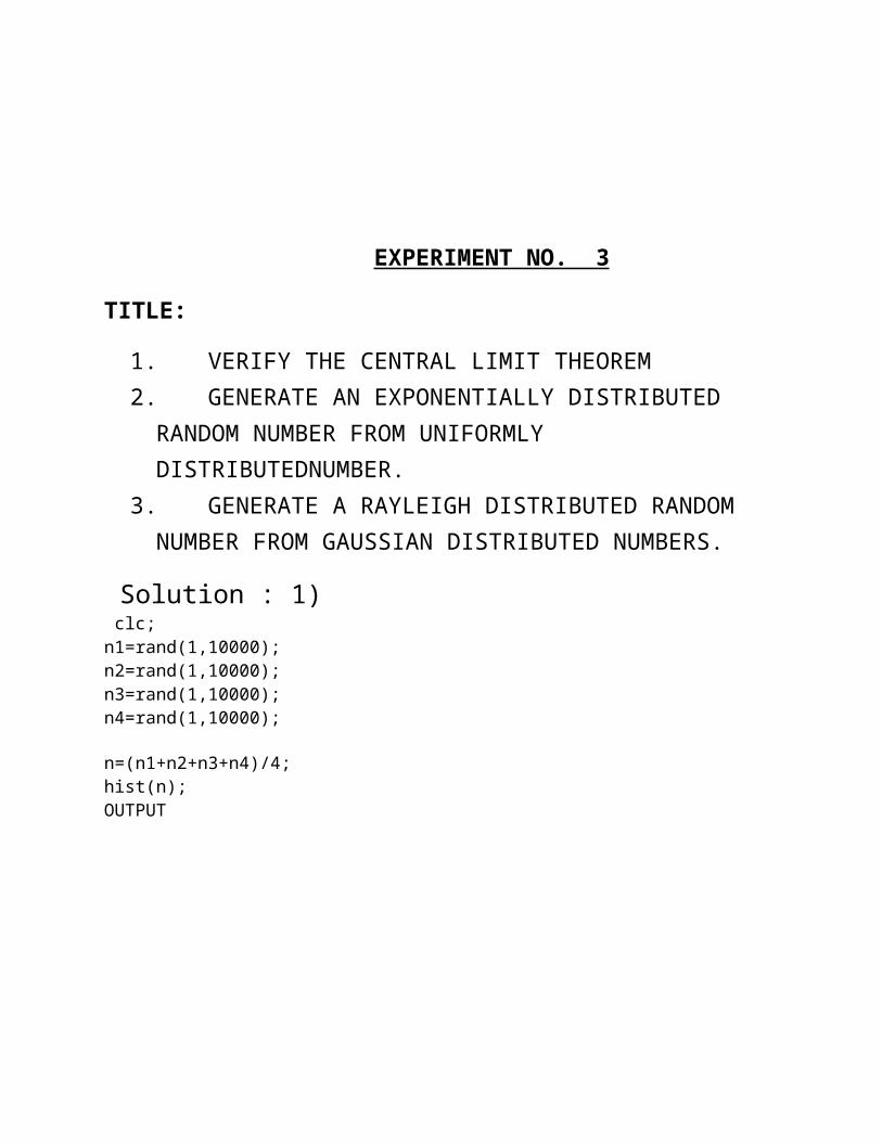
EXPERIMENT NO. 3
TITLE:
1. VERIFY THE CENTRAL LIMIT THEOREM2. GENERATE AN EXPONENTIALLY DISTRIBUTED
RANDOM NUMBER FROM UNIFORMLY DISTRIBUTEDNUMBER.
3. GENERATE A RAYLEIGH DISTRIBUTED RANDOM NUMBER FROM GAUSSIAN DISTRIBUTED NUMBERS.
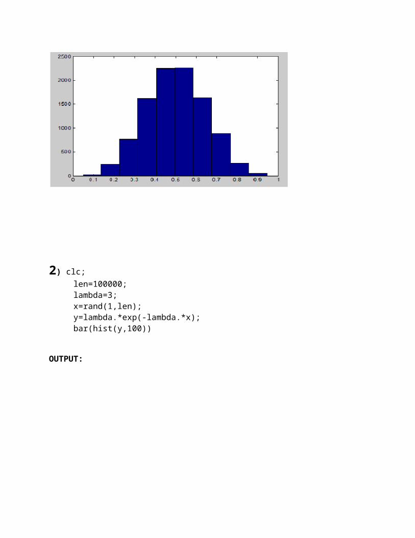
Solution : 1) clc;n1=rand(1,10000);n2=rand(1,10000);n3=rand(1,10000);n4=rand(1,10000); n=(n1+n2+n3+n4)/4;hist(n);OUTPUT
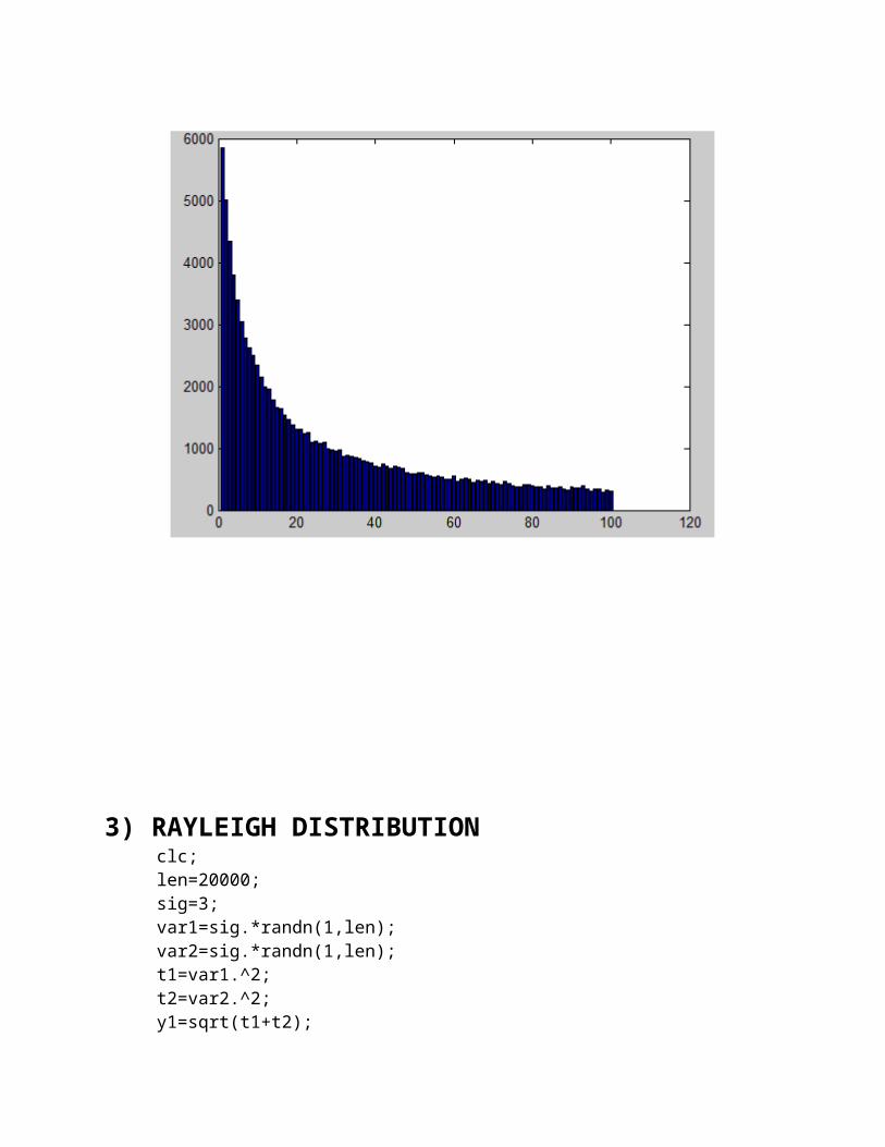
2) clc;
len=100000; lambda=3; x=rand(1,len); y=lambda.*exp(-lambda.*x); bar(hist(y,100))
OUTPUT:
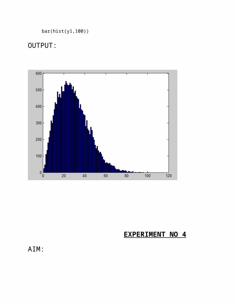
3) RAYLEIGH DISTRIBUTIONclc;len=20000;
sig=3;var1=sig.*randn(1,len);var2=sig.*randn(1,len);t1=var1.^2;t2=var2.^2;y1=sqrt(t1+t2);bar(hist(y1,100))
OUTPUT:
EXPERIMENT NO 4
AIM:
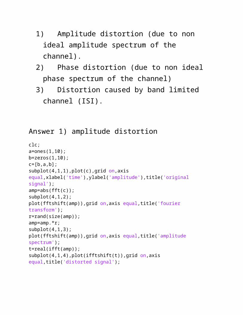
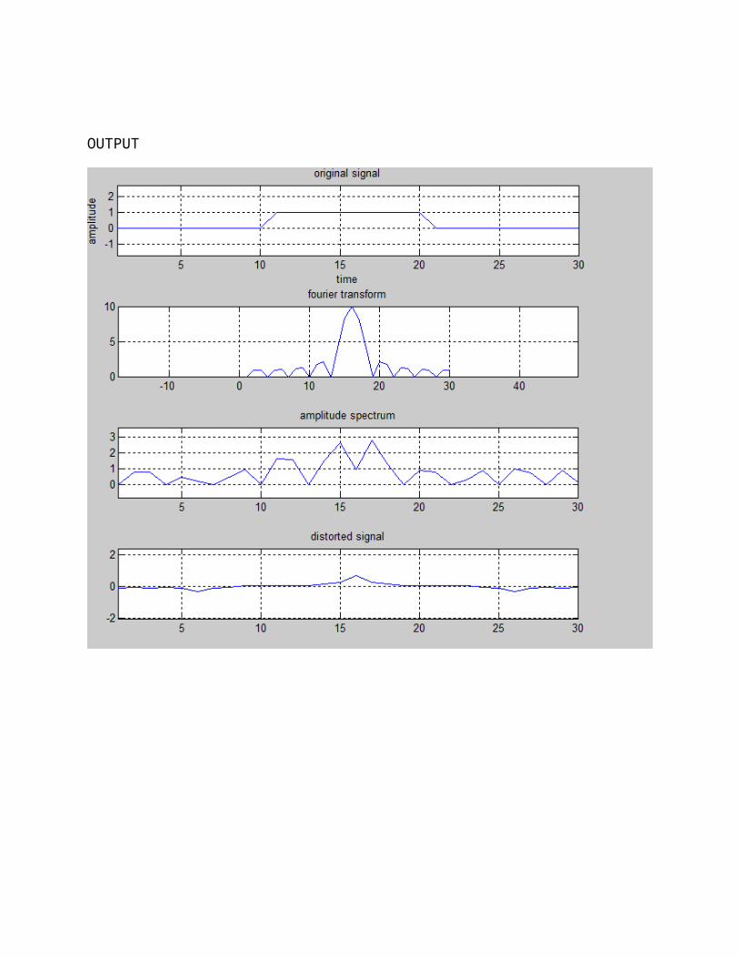
1) Amplitude distortion (due to non ideal amplitude spectrum of the channel).
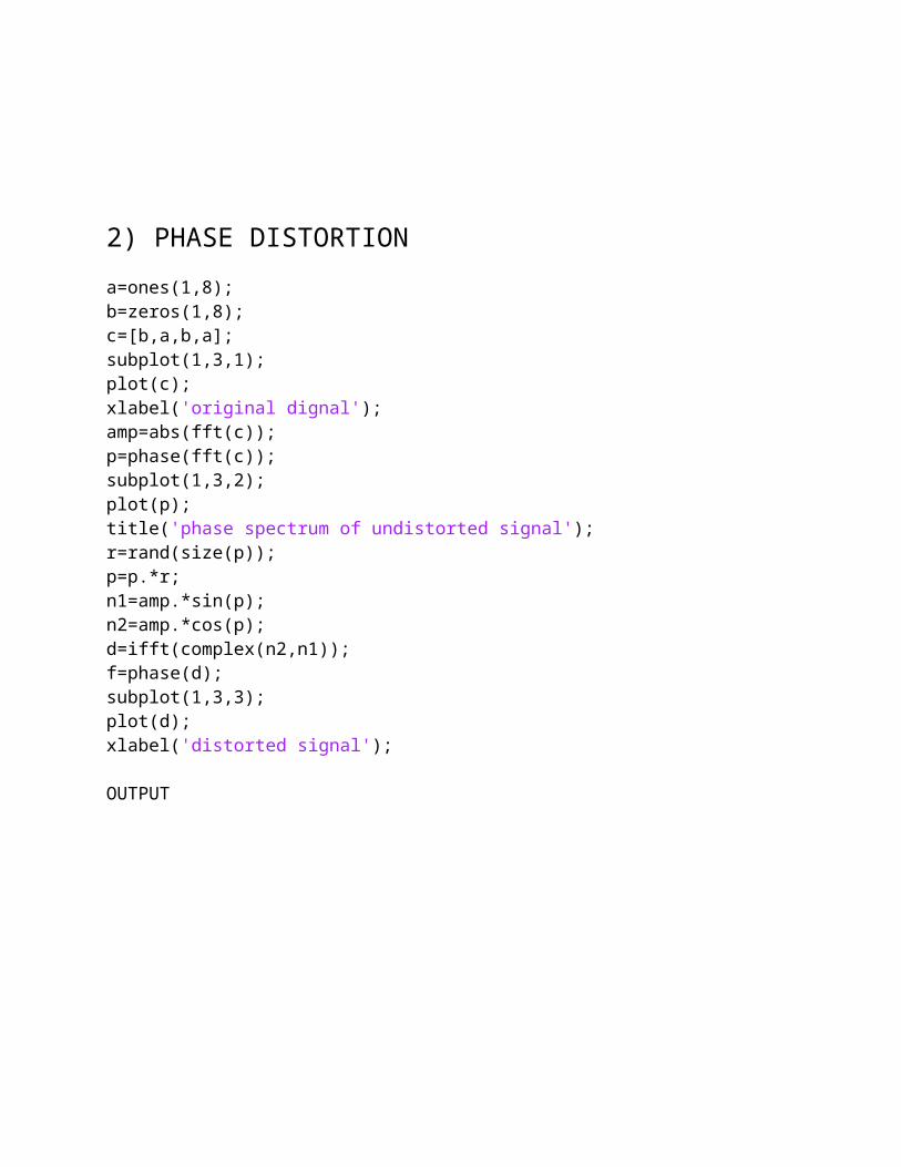
2) Phase distortion (due to non ideal phase spectrum of the channel)
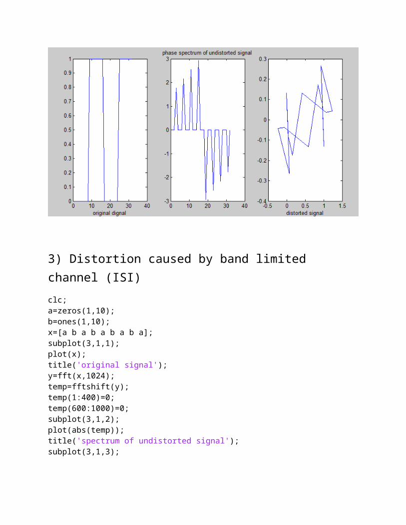
3) Distortion caused by band limited channel (ISI).
Answer 1) amplitude distortion
clc;a=ones(1,10);b=zeros(1,10);c=[b,a,b];subplot(4,1,1),plot(c),grid on,axis equal,xlabel('time'),ylabel('amplitude'),title('original signal');amp=abs(fft(c));subplot(4,1,2);plot(fftshift(amp)),grid on,axis equal,title('fourier transform');r=rand(size(amp));amp=amp.*r;subplot(4,1,3);plot(fftshift(amp)),grid on,axis equal,title('amplitude spectrum');t=real(ifft(amp));subplot(4,1,4),plot(ifftshift(t)),grid on,axis equal,title('distorted signal');
OUTPUT
2) PHASE DISTORTION
a=ones(1,8);b=zeros(1,8);c=[b,a,b,a];subplot(1,3,1);plot(c);xlabel('original dignal');amp=abs(fft(c));p=phase(fft(c));subplot(1,3,2);plot(p);title('phase spectrum of undistorted signal');r=rand(size(p));p=p.*r;n1=amp.*sin(p);n2=amp.*cos(p);d=ifft(complex(n2,n1));f=phase(d);subplot(1,3,3);plot(d);xlabel('distorted signal');
OUTPUT
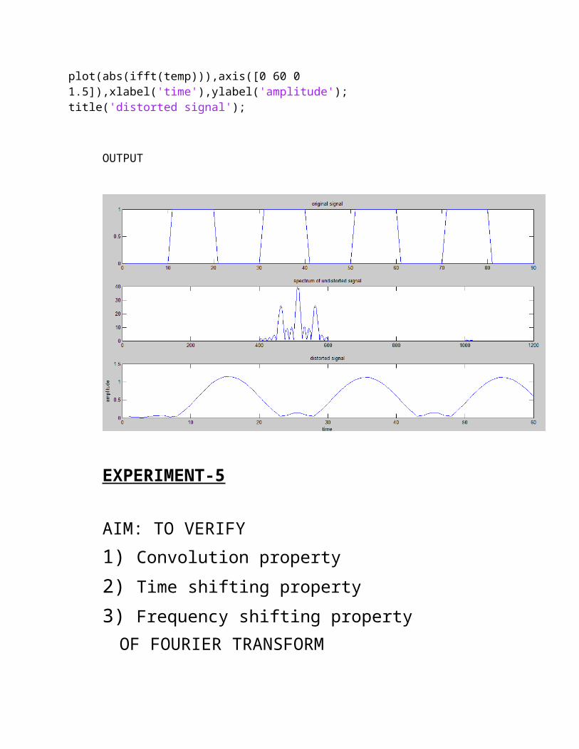
3) Distortion caused by band limited channel (ISI)
clc;a=zeros(1,10);b=ones(1,10);x=[a b a b a b a b a];subplot(3,1,1);plot(x);title('original signal');y=fft(x,1024);temp=fftshift(y);temp(1:400)=0;temp(600:1000)=0;subplot(3,1,2);plot(abs(temp));title('spectrum of undistorted signal');subplot(3,1,3);plot(abs(ifft(temp))),axis([0 60 0 1.5]),xlabel('time'),ylabel('amplitude');title('distorted signal');
OUTPUT
EXPERIMENT-5
AIM: TO VERIFY1) Convolution property
2) Time shifting property
3) Frequency shifting propertyOF FOURIER TRANSFORM
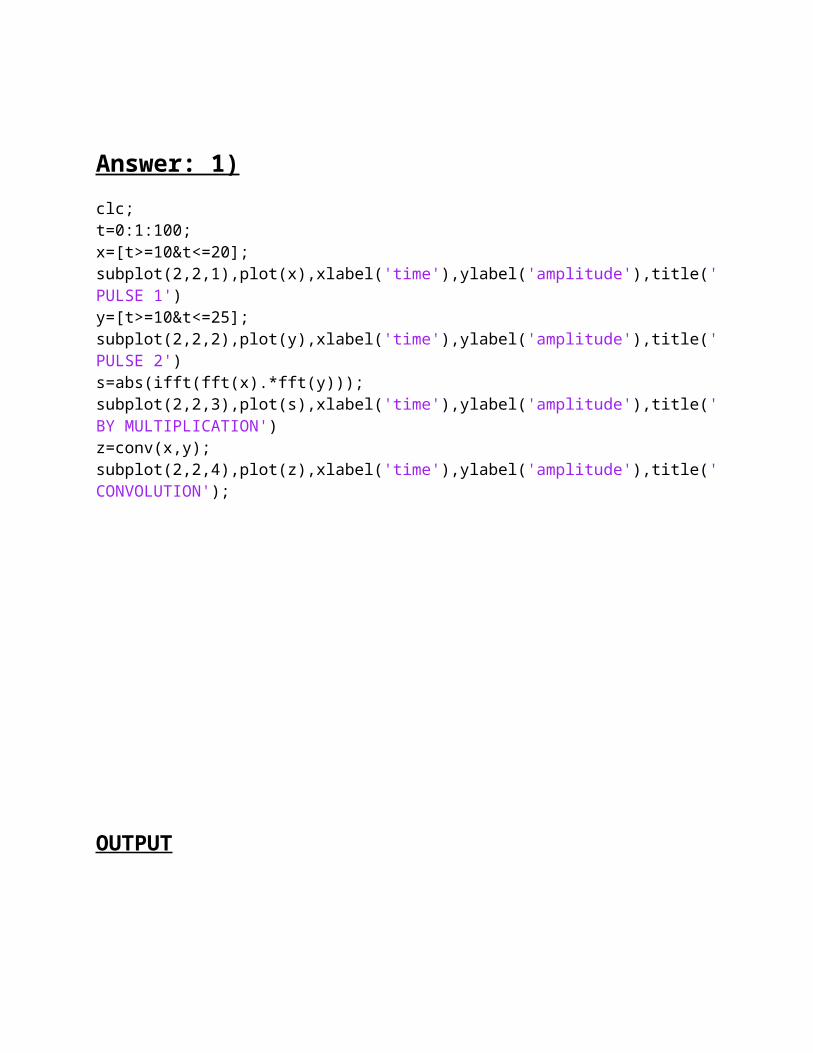
Answer: 1)
clc;t=0:1:100;x=[t>=10&t<=20];subplot(2,2,1),plot(x),xlabel('time'),ylabel('amplitude'),title('PULSE 1')y=[t>=10&t<=25];subplot(2,2,2),plot(y),xlabel('time'),ylabel('amplitude'),title('PULSE 2')s=abs(ifft(fft(x).*fft(y)));subplot(2,2,3),plot(s),xlabel('time'),ylabel('amplitude'),title('BY MULTIPLICATION')z=conv(x,y);subplot(2,2,4),plot(z),xlabel('time'),ylabel('amplitude'),title('CONVOLUTION');
OUTPUT
2)
clc;a=ones(1,128)b=zeros(1,128)pulse=[b a b a b];subplot(2,1,1),plot(pulse),xlabel('time'),ylabel('amp'),title('PULSE');fftpulse=fftshift(fft(pulse,256));for n=1:1:256 c(n)=fftpulse(n).*exp((128*j*2*pi*n)/256);endd=abs(ifft(c));subplot(2,1,2),plot(d),xlabel('time'),ylabel('amp'),title('TIME SHIFTING');
OUTPUT
3)
clc;a=ones(1,90)b=zeros(1,90)pulse=[b a b];subplot(2,2,1),plot(pulse),xlabel('time'),ylabel('amplitude'),title('PULSE');fftpulse=fftshift(fft(pulse,256));subplot(2,2,2),plot(abs(fftpulse)),xlabel('frequency'),ylabel('amplitude'),title('FOURIER TRANSFORM')for n=1:1:128 c(n)=pulse(n).*exp((90*j*2*pi*n)/256);endd=(fftshift(fft(c,256)))subplot(2,2,3),plot(abs(d)),xlabel('frequency'),ylabel('amplitude'),title('SPECTRUM');OUTPUT