Addendum to

CFLE Theory, Revised Edition

RELATION BETWEEN QUANTUM CHROMODYNAMICS AND THE

GENERAL RELATIVITY OF CFLE THEORY

1. The Proton Spin Crisis

According to the generally accepted Standard Model (Quark-Parton Model), there are two types of quarks in the proton (or nucleon)—one

with spin + (known as the “up” quark) and the other with spin −

(the “down” quark). Current theoretical physicists assume the proton to

have a total spin of + along some axis, comprising two “up” and one

“down” quark particles. That is, + = + + + + − 1-1

In 1987, the European Muon Collaboration (EMC), which had been scattering muons off polarized protons at CERN, imploded the particle physics community with their experimental news that not enough of the proton’s spin could be contributed by the spin of its three constituent quarks. In other words, the overall quark contribution to the proton is only

Δ Σ = (12±9±14) % 1-2

This result was called the EMC effect, and it precipitated what became known as the “Proton Spin Crisis.”

Following the 1987 report, the EMC spent a further 30 years continuing the experiments at CERN. Concurrently, researches were being done by the Jefferson Lab and RHIC at Brookhaven National Laboratory, the HERMES experiment at DESY Laboratory, and the COMPASS experiment at CERN. It was found in experiments that the number of quarks with spin in the proton’s spin direction was almost the same as the number of quarks whose spin was is in the opposite direction. Global analysis of data from all major experiments confirmed that the quark spin contributed only about 30% to the total spin of the proton (nucleon). That is,

2 Addendum to CFLE Theory, Revised Ed.

ΔΣ~30% 1-3

Therefore, it was believed that the remaining spin must be carried by a gluon and orbital angular momentum. Consequently, the related sum rule of the proton spin was changed to

= ∆Σ + ∆ + 1-4

where ∆Σ is the quark spin, ∆ is the gluon spin, and is the orbital angular momentum.

Data on quark and gluon distributions have shown that ∆Σ = ∆Σ( , ) 1-5

(where Q2 is the squared 4-momentum-transfer vector q of the exchanged virtual particle and x is the “Bjorken x” scaling variable) is

constrained, but ∆ = ( , ) d is largely unknown.

Experiments were (and are still being) continued to verify the particle contributions to the nucleon spin, and some current data have suggested that the valence quarks could make up ~60% of the nucleon’s spin.

Descriptions of the experiments done and data collected over the past 30 years, as well the postulates and calculations behind the experiments (i.e., spin-dependent Parton density functions, sum rules and spin polarizability, quark-hadron duality, spin structure functions g1 and g2 and their moments, etc.), have already been published elsewhere, and do not need repeating here. [An excellent review is given by Kuhn SE et al., “Spin Structure of the Nucleon – Status and Recent Results,” February 11, 2009. Accessible at http://arxiv.org/pdf/0812.3535.pdf ]

Sufficed to say that, in spite of the global efforts to reconcile data with theory, the crisis remained that part of the proton’s spin lay elsewhere. As summarized by Kuhn et al.,

“Measurements of the polarized gluon density suggest that it is much too small to resolve the spin crisis.”

But the essence of the proton spin crisis is that current physicists cannot understand why the value of ∆Σ can be 30%. CFLE theory (discussed below) will prove that this 30% result is not such a crisis at all.

Addendum to CFLE Theory, Revised Ed. 3

2. Similarities Between the Missing Precession of Planet Mercury and the Missing Spin of the Valence Quark

In Chapter 1 of my book, I touched briefly on the precession of planet Mercury. It was Urbain Le Verrier (1811–1877) who discovered the missing precession of Mercury’s perihelion in 1843, when he observed Mercury’s motion around the Sun to be 574 arcsec per century. To account for this value using Newtonian mechanics, he totaled up the contributions made by the other known planets in our solar system to Mercury’s precession. Venus contributed 277 arcsec, 153 arcsec was by Jupiter, 90 arcsec by Earth, and 10 arcsec by Mars and the remaining planets combined, for a total of 531 arcsec per century. This left 43 arcsec unaccounted for, giving rise to the crisis of “Mercury’s missing precession.”

This discovery shone a huge spotlight on the limits of Newtonian celestrial mechanics and, along with many other unresolved physics phenomena, signaled the need for some new physics concepts in the 19th century. From 1859 to 1915, many explanations of Mercury’s missing perihelion precession were put forward, but all fell by the wayside. It was Einstein, in November 1915, who would eventually glean the magical number of 43 arcsec per century out of one of the first calculations from his new general relativity theory.

From the viewpoint of the general relativity of curved force line elements theory, we can find that the proton spin crisis is very similar to the Mercury precession crisis. As discussed in my book, Einstein’s general relativity theory cannot be extended to the strong force as well as the weak force and electromagnetic force. Because Einstein’s general relativity is entrenched in curved space and extra dimensions, his theory becomes incalculable and unextendable to these three forces.

Modern physicists also do not have a calculable general relativity for each force and it related phenomena. Therefore, such physics crises remain unresolved.

CFLE theory, on the other hand, is calculable and extendable to every known force, so this theory can identify similarities between the proton spin crisis and mercury’s missing precession problem:

● Le Verrier and the Paris observatory ⇛ All members of the EMC and the EMC at CERN

● The solar system ⇛ the proton system

4 Addendum to CFLE Theory, Revised Ed.

● The planet Mercury ⇛ the valence quarks

● The other planets ⇛ gluon and other quarks

● Mercury’s missing precession ⇛ missing quark spin

● The numerous proposals ⇛ the numerous sum rules

● Newtonian celestial mechanics ⇛ quantum chromodynamics

● No calculable theory of general relativity for gravitational interaction ⇛ no calculable theory of general relativity for electromagnetic interaction and strong interaction

3. Relation Between Quantum Mechanics and CFLE Theory

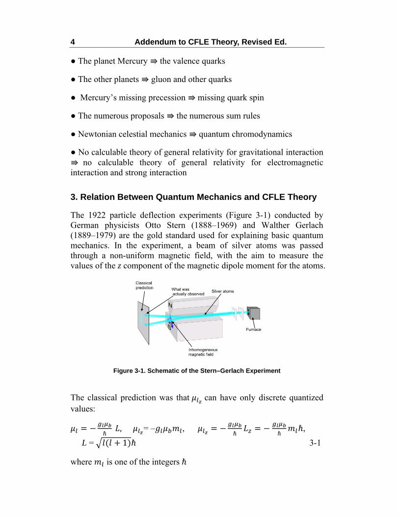
The 1922 particle deflection experiments (Figure 3-1) conducted by German physicists Otto Stern (1888–1969) and Walther Gerlach (1889–1979) are the gold standard used for explaining basic quantum mechanics. In the experiment, a beam of silver atoms was passed through a non-uniform magnetic field, with the aim to measure the values of the z component of the magnetic dipole moment for the atoms.

Figure 3-1. Schematic of the Stern–Gerlach Experiment

The classical prediction was that can have only discrete quantized values: = − ℏ , = – , = − ℏ = − ℏ ℏ,

L = ( + 1)ℏ 3-1

where is one of the integersℏ

Addendum to CFLE Theory, Revised Ed. 5

= – , − + 1,… ,0, …+ − 1,+ 3-2

Thus, as seen in Figure 3-1 (and Figure 3-2), the deflected beam was predicted to be spread into a continuous band that corresponds to a continuous distribution of from each atom. Instead, the beam pattern was split into a positive z component and a negative z component (Figures 3-1 and 3-3).

Figure 3-2. Classically predicted Figure 3-3. Observed

This suggested the existence of some other unknown magnetic dipole moment in the atom. Samual Goudsmit (1902–1978) and George Uhlenbeck (1900–1988) theorized that the magnitude S and the z component ( ) of the spin angular momentum were related to two quantum numbers, s and ms, by the same quantization relation as those for orbital angular momentum. That is

L = ( + 1)ℏ → S = ( + 1)ℏ, = ℏ 3-3

= − ℏ → = − ℏ 3-4

= − → = − 3-5

Experimentally, = ±1 3-6

Because the beam of silver atoms is deflected into two equal and opposite z components, it stands to reason that can assume just two values, equal in magnitude but opposite in sign. Therefore,

= − ,+ 3-7

and s has the single value

s = 3-8

6 Addendum to CFLE Theory, Revised Ed.

From Eq. 3-6, the possible value of gs is

= 2 3-9

Spectroscopic measurements of Lamb, using a technique of extra accuracy, have actually shown that

= 2.00232 3-10

According to CFLE theory, this value is none other than the degree of the curved force line g, like the degree of curved space in the classical theory of general relativity.

From §7 of my book, the minimum g value of a proton is given as

= 6.545979 3-11

Extrapolating from Eq. 3-6, therefore, the possible value of is = ±1, 6.545979 = ±1 3-12

Thus, the possible value of is

= − . , + . 3-13

The related that has a single value (cf. Eq. 3-8) is

= . 3-14

The permitted magnitude of the proton’s constituents and its permitted spin angular momentum are

= ( + 1)ℏ 3-15

= ℏ = ± . ℏ 3-16

This final permitted value of for the proton’s constituents can be compared to the typical value of (the fermion’s spin angular momentum according to the Standard Model)

Addendum to CFLE Theory, Revised Ed. 7

= ±( . )ℏ±( )ℏ =

. ℏ. ℏ = 0.3 = 30% 3-17

∆Σ = ∆Σ( , ) ~ 30% 1-5

This theoretical value of CFLE theory agrees very well with the experimental value of the proton’s valence quarks spin from all the laboratories on Earth.

4. Relation Between General Relativity and Quantum Chromodynamics

The Gravity Probe B satellite was designed to test one of the predictions of Einstein’s general theory of relativity: the effect of the curvature of space–time on a body (vector) moving along the same surface as an orbiting body such as Earth—otherwise known as the geodetic effect. The phenomenon can be visualized as Earth sitting on and creating a dent in a trampoline, such that a gyroscope (like the one carried by GP-B) moving along the trampoline surface will be naturally drawn down the warped slope towards Earth (Figure 4-1).

Figure 4-1

Francis Everitt, the principal investigator of GP-B, also describes the geodetic effect as the so-called “missing inch” (Figure 4-2).

8 Addendum to CFLE Theory, Revised Ed.

Figure 4-2

In this alternative view, we consider a circle with the same diameter (D) as Earth’s (~7,900 miles) existing in empty space. Standard Euclidian geometry would put the circle’s diameter as π × D (~24,800 miles). The gyroscope following this circular path in empty space would always point in the same direction, as Figure 4-2left illustrates. Now, were we to slip Earth inside of this circle, Earth’s mass would warp the space–time inside the circle into a shallow cone, shrinking the circumference of the circle by a mere 1.1 inches.

We can visualize this effect by cutting out a pie-shaped wedge from the circle and closing the gap, as illustrated in Figure 4-3.

Figure 4-3

The circumference of the resulting cone is slightly diminished, and the orientation of the moving gyroscope shifts as shown in Figure 4-3right. Measuring this shifting orientation of the gyroscope’s spin axis as it

Addendum to CFLE Theory, Revised Ed. 9

moves through warped space–time is the essence of the GP-B experiment.

By correlating the geodetic effect with the proton spin value, we can understand why the valence quarks’ spin is smaller than expected for a proton. When we liken the spin of the proton to the spin of the gyroscope in the GP-B experiment, Figure 4-3left corresponds to the bound (flat) state of the proton, g = 2.

Now, the orientation of a single gyroscope can only be one, but were we to test many gyroscopes, the orientation of each gyroscope would be different. Likewise, testing the spin of several proton constituents in each location in the EMC experiments would give many different spin orientations, like Figure 4-3right (the curved state, or g = 6.545979).

Figure 4-4 shows qualitatively and more simply how a curved system produces different orientations of gyroscopes or different spin orientations of a proton’s constituent particles. When the proton is in the bound state, the whole sytem is flat relative to the base line of the rest frame. All spin components have only one orientation (Figure 4-4left). When the proton system decays as constituent particles under the given degree of curved force line g = 6.545979, the whole system is curved relative to the base line of the rest frame.

Figure 4-4

In such condition, the spin orientation of each constituent particle is different by as much as the degree of the curved force line (Figure 4-4right). Qualitatively, this is the same as the “missing inch” effect, which is why the valence quarks’ spin is smaller than expected for a proton.

∆Σ = ∆Σ( , ) ~ 30% 1-5

10 Addendum to CFLE Theory, Revised Ed.

Equation 3-17 shows that the general relativity of CFLE theory is quantitatively correct too:

= ±( . )ℏ±( )ℏ =

. ℏ. ℏ = 0.3 = 30% 3-17

5. Conclusion

This agreement in calculated and observed values leads to my conviction that the general relativity of CFLE theory is correct and extendable to each known physical force.

In the Standard Model, fermions’ spin increases discretely as = ± ,± ,± ,± ,± ,± ,± …. 5-1

But, in CFLE theory, fermions’ spin can decrease discretely as

= ± , ± , ± , ± , ± , ± …

= ± ,± . , ± . , ± . , ± . , ± . … 5-2

Therefore, the permitted spin of the proton’s constituent particles (valence quarks) over g = 6.545979 as fermions is = ± ,±

= ± . , ± . 5-3

The sum rule of valence quarks for building the proton system (at maximum permitted force line gradient of g = 2) is

= + . + . − . = . = . ≈ 5-4

The sum rule for building up the neutron (maximum permitted force line gradient of g = 2) is

= − . − . − . = . = . ≈ 5-5

Addendum to CFLE Theory, Revised Ed. 11

Finally, the possible permitted sum rule of the constituent state for the proton (permitted maximum force line gradient of g = 6.545979) is

=+ . − . + . = . = 0.15 ≈ 30% 5-6

=+ . − . + . = . = 0.15 ≈ 30% 5-7

Expressing Figure 4-4 directly with force line elements only gives Figure 5-1.

Figure 5-1

According to CFLE theory, in Figure 5-1 we can find that when the force line element is curved, the static electric charge is decreased, as discussed in §6. Therefore, the number of related magnetic force lines for the angular momentum and spin angular momentum, according to Eqs. 3-1, 3-4, and 3-5, is also decreased.

However, the static electric charge of an “up” quark is = + ( + ) = + + + 0 = + 5-8

Those of the “down” quark and “strange” quark are

= + ( + ) = − + + 0 = −

= 0 + − 1 = − 5-9

Therefore, according to CFLE theory, the permitted maximum spin of an “up” quark is

= ( )(+ ) = + ≈ + . 5-10

12 Addendum to CFLE Theory, Revised Ed.

and that of the “down” quark and “strange” quark is

, = ( )(− ) = − ≈ − . 5-11

This result means that the possible quarks spin are ± ± , not ± ,

despite that quarks are fermions.

In conclusion:

● The Standard Model of particle physics is incorrect.

● The permitted sum rule for the bound state of a proton should be 12 = ∆Σ = Δ + Δ − Δ

● The permitted sum rule for the constituent state of a proton should be 16.5 = ∆Σ = ±Δ ± Δ ± Δ