NREL is a national laboratory of the US Department of Energy Office of Energy Efficiency amp Renewable Energy Operated by the Alliance for Sustainable Energy LLC This report is available at no cost from the National Renewable Energy Laboratory (NREL) at wwwnrelgovpublications

Contract No DE-AC36-08GO28308

Adding Complex Terrain and Stable Atmospheric Condition Capability to the OpenFOAM-based Flow Solver of the Simulator for OnOffshore Wind Farm Applications (SOWFA) Preprint Matthew J Churchfield Sang Lee and Patrick J Moriarty Presented at the 1st Symposium on OpenFOAM in Wind Energy Oldenburg Germany March 20-21 2013

Conference Paper NRELCP-5000-58539 September 2013

NOTICE

The submitted manuscript has been offered by an employee of the Alliance for Sustainable Energy LLC (Alliance) a contractor of the US Government under Contract No DE-AC36-08GO28308 Accordingly the US Government and Alliance retain a nonexclusive royalty-free license to publish or reproduce the published form of this contribution or allow others to do so for US Government purposes

This report was prepared as an account of work sponsored by an agency of the United States government Neither the United States government nor any agency thereof nor any of their employees makes any warranty express or implied or assumes any legal liability or responsibility for the accuracy completeness or usefulness of any information apparatus product or process disclosed or represents that its use would not infringe privately owned rights Reference herein to any specific commercial product process or service by trade name trademark manufacturer or otherwise does not necessarily constitute or imply its endorsement recommendation or favoring by the United States government or any agency thereof The views and opinions of authors expressed herein do not necessarily state or reflect those of the United States government or any agency thereof

This report is available at no cost from the National Renewable Energy Laboratory (NREL) at wwwnrelgovpublications

Available electronically at httpwwwostigovbridge

Available for a processing fee to US Department of Energy and its contractors in paper from

US Department of Energy Office of Scientific and Technical Information PO Box 62 Oak Ridge TN 37831-0062 phone 8655768401 fax 8655765728 email mailtoreportsadonisostigov

Available for sale to the public in paper from

US Department of Commerce National Technical Information Service 5285 Port Royal Road Springfield VA 22161 phone 8005536847 fax 7036056900 email ordersntisfedworldgov online ordering httpwwwntisgovhelpordermethodsaspx

Cover Photos (left to right) photo by Pat Corkery NREL 16416 photo from SunEdison NREL 17423 photo by Pat Corkery NREL 16560 photo by Dennis Schroeder NREL 17613 photo by Dean Armstrong NREL 17436 photo by Pat Corkery NREL 17721

Printed on paper containing at least 50 wastepaper including 10 post consumer waste

NOTICE

The submitted manuscript has been offered by an employee of the Alliance for Sustainable Energy LLC (Alliance) a contractor of the US Government under Contract No DE-AC36-08GO28308 Accordingly the US Government and Alliance retain a nonexclusive royalty-free license to publish or reproduce the published form of this contribution or allow others to do so for US Government purposes

This report was prepared as an account of work sponsored by an agency of the United States government Neither the United States government nor any agency thereof nor any of their employees makes any warranty express or implied or assumes any legal liability or responsibility for the accuracy completeness or usefulness of any information apparatus product or process disclosed or represents that its use would not infringe privately owned rights Reference herein to any specific commercial product process or service by trade name trademark manufacturer or otherwise does not necessarily constitute or imply its endorsement recommendation or favoring by the United States government or any agency thereof The views and opinions of authors expressed herein do not necessarily state or reflect those of the United States government or any agency thereof

This report is available at no cost from the National Renewable Energy Laboratory (NREL) at wwwnrelgovpublications

Available electronically at httpwwwostigovbridge

Available for a processing fee to US Department of Energy and its contractors in paper from

US Department of Energy Office of Scientific and Technical Information PO Box 62 Oak Ridge TN 37831-0062 phone 8655768401 fax 8655765728 email mailtoreportsadonisostigov

Available for sale to the public in paper from

US Department of Commerce National Technical Information Service 5285 Port Royal Road Springfield VA 22161 phone 8005536847 fax 7036056900 email ordersntisfedworldgov online ordering httpwwwntisgovhelpordermethodsaspx

Cover Photos (left to right) photo by Pat Corkery NREL 16416 photo from SunEdison NREL 17423 photo by Pat Corkery NREL 16560 photo by Dennis Schroeder NREL 17613 photo by Dean Armstrong NREL 17436 photo by Pat Corkery NREL 17721

Printed on paper containing at least 50 wastepaper including 10 post consumer waste

Adding Complex Terrain and Stable Atmospheric Condition Capability to the OpenFOAM-based Flow Solver of the Simulator

for OnOffshore Wind Farm Applications (SOWFA)

Matthew J Churchfield Sang Lee Patrick J Moriarty

Thursday 12th September 2013

Abstract

The National Renewable Energy Laboratoryrsquos Simulator for OnOffshore Wind Farm Applications contains an OpenFOAM-based flow solver for performing large-eddy simulation of flow through wind plants The solver comshyputes the atmospheric boundary layer flow and models turbines with actuator lines Until recently the solver was limited to flows over flat terrain and could only use the standard Smagorinsky subgrid-scale model In this work we present our improvements to the flow solver that enable us to 1) use any OpenFOAM-standard subgrid-scale model and 2) simulate flow over complex terrain We used the flow solver to compute a stably stratified atmospheric boundary layer using both the standard and the Lagrangian-averaged scale-independent dynamic Smagorinsky models Surprisingly the results using the standard Smagorinsky model compare well to other researchersrsquo results of the same case although it is often said that the standard Smagorinsky model is too dissipative for accurate stable stratification calculations The scale-independent dynamic subgrid-scale model produced poor results probably due to the spikes in model constant with values as high as 46 We applied a simple bounding of the model constant to remove these spikes which caused the model to produce results much more in line with other researchersrsquo results We also computed flow over a simple hilly terrain and performed some basic qualitative analysis to verify the proper operation of the terrain-local surface stress model we employed

1 Introduction In this work we present improvements to the OpenFOAM-based Simulator for OnOffshore Wind Farm Applishycations (SOWFA) that is being continually developed at the US Department of Energyrsquos National Renewable Energy Laboratory (NREL) SOWFA is composed of an OpenFOAM-based incompressible atmosphericwind farm large-eddy simulation (LES) solver that models turbines as actuator lines coupled with NRELrsquos FAST wind turbine structural and system dynamics model An example of a flow computed with SOWFA is that of the 48-turbine Lillgrund offshore wind farm that lies between Sweden and Denmark [1]

Until recently SOWFA was limited to computing wind farm flow over flat terrain under neutral or unstable atshymospheric conditions The flat terrain limitation existed because we had implemented planetary surface shear stress and temperature flux models commonly used in the atmospheric LES community that rely on Monin-Obukhov similarity theory The surface stress models assume flat homogeneous terrain over which a planar average wind profile is calculated that is then used to determine the average planetary surface stress The limitation that only neushytral and unstable atmospheric conditions could be simulated was due to the fact that the flow solver relied on a cell face-based subgrid-scale (SGS) viscosity formulation which deviates from the OpenFOAM-standard cell-centered turbulence variable approach This means that the OpenFOAM-standard SGS models were not compatible with our custom LES solver Because of its simplicity we implemented only the standard Smagorinsky model into this nonshystandard face-based SGS formulation but Brown et al [2] showed that the standard Smagorinsky model does not perform as well as models with backscatter in simulating stable atmospheric flow Furthermore Beare et al [3] have shown that at typical grid resolution SGS models more sophisticated than the standard Smagorinsky model are able to better capture stable atmospheric boundary layer details Also the Lagrangian-averaged scale-dependent dynamic Smagorinsky model of Stoll and Porteacute-Agel [4] has been shown to perform well in stably stratified atmospheric flows [5]

1

This report is available at no cost from the National Renewable Energy Laboratory at wwwnrelgovpublications

To circumvent these limitations we implemented a local planetary surface stress model that does not require horizontal averages in a plane of homogeneity following the work of Wan and colleagues [6] This allows the solver to compute flow over irregular terrain To create a terrain-conforming mesh we use OpenFOAMrsquos moveshyDynamicMesh solver We also migrated back to the standard OpenFOAM cell-centered SGS viscosity approach and the results are very similar to our previous face-centered SGS stress approach meaning that the entire suite of standard OpenFOAM SGS models can now be used with our atmosphericwind farm flow solver including the Lagrangian-averaged scale-independent dynamic Smagorinsky model of Meneveau and colleagues [7]

With these enhancements to the SOWFA flow solver we computed the well-documented stably stratified atmospheric boundary layer computed in the Global Energy and Water Cycle Experiment (GEWEX) Atmospheric Boundary Layer Study (GABLS) model intercomparison [3] We also computed the flow of a neutral boundary layer capped with an inversion over a simple hilly terrain

We are interested in simulating stably stratified flow because it can be one of the most damaging flows for wind turbines Kelley [8] spent many years at NREL researching the effects of the stable atmospheric boundary layer (ABL) on wind turbines His study shows that much wind turbine damage occurs in weakly stable flow Stable ABL flows are characterized by lower and sometimes intermittent turbulence levels and strong vertical shear of wind speed and direction both of which cause considerable fatigue loads on modern turbine rotors with a span on the order of 100 m The lower turbulence levels mean that turbine wakes persist for longer distances downstream and hence can decrease the efficiency of a wind plant The stable ABL can also contain a low-level jet a layer of flow that has speed greater than the flow above the ABL Gravity waves can also form All of these unique features of the stably stratified ABL make it important and challenging to simulate accurately

Flow through complex terrain is important because effects like local acceleration separation and recirculation can occur all of which have important impacts on turbines located within the terrain Although many wind plants are located in flat regions such as those in the U S Midwest region there is a significant number of farms located in complex terrain Complex terrain remains a challenge for reduced-order flow models used by wind plant layout engineers so having an accurate computational tool would help to improve these reduced-order tools

11 History of Subgrid-Scale Models Suitable for the Stable Atmospheric Boundary Layer and Terrain Subgrid-scale models are an important part of LES of the ABL Near the lower surface where the turbulent scales are constrained and the largest resolved eddies become smaller than at greater distances from the surface the influence of the SGS model is more dominant than at greater distances from the surface The same is true of LES of stable ABLs Because buoyancy forces act to suppress turbulence in those cases the largest resolved scales are smaller than those resolved in LES of neutral or unstable ABLs SGS models often assume that the subgrid scales of turbulence are fairly isotropic which is not true of the near-wall or stable ABL subgrid scales for typical grid resolutions Dynamic SGS models have been seen as an improvement over static models but they rely on some type of averaging which often is done in the direction of homogeneity In flow over complex terrain there is no direction of homogeneity so again a well-designed SGS model is important Because of their important role in LES of the ABL we will discuss the lineage of SGS models that have led to some of todayrsquos most sophisticated models that are used for LES of the stable ABL and of the ABL over terrain

In performing LES of the ABL often the incompressible filtered Navier-Stokes equations are solved using the Boussinesq approximation for buoyancy along with the continuity equation which is usually enforced through the solution of an elliptic equation for the pressure variable The continuity equation is

partUi

partxi = 0 (1)

and the momentum equation is

part Ui

part t +

part U j Ui

partx j = minus2εi3kΩ Uk minus

part p partxi

minus τi j

partx j +ρbgi (2)

In these equations the over line denotes the LES filtering operation Ui is the component of the resolved-scale velocity vector in the coordinate direction xi εi jk is the alternating unit tensor Ω is the planetary rotation rate vector at the point of interest on the planet (which is dependent on latitude) p is pressure τi j is the SGS stress tensor ρb is a scalar that dictates the sign and strength of the buoyancy force and gi is the gravitation vector In order to compute ρb which is given by

macr θ minusθ0

ρb = 1minus (3)

θ0

2

This report is available at no cost from the National Renewable Energy Laboratory at wwwnrelgovpublications

where θ is the resolved-scale potential temperature and θ0 is a reference temperature a potential temperature transport equation must be solved and is given by

part macr part macr macrθ Ujθ τθ i + = minus (4) part t partx j partxi

where τθ i is the SGS temperature flux In both the momentum and potential temperature equations the effects of molecular diffusion are not included because the SGS effects are much more dominant except very near the surface Near the surface LES of the ABL nearly always relies on some sort of surface model in which viscous and SGS stresses and temperature fluxes are lumped together

The SGS stress tensor arises from the filtering of the Navier-Stokes equations The first term of the right-hand side of τi j = UiUj minusUiUj cannot be directly solved so τi j must be modeled The majority of SGS models rely upon macr

the linear eddy-viscosity assumption that the SGS stress found in Eq 2 is related to resolved-scale strain by

macrτi j D = minus2νt Si j (5)

where τi j D is the deviatoric SGS stress tensor (in practice the isotropic part can be absorbed into the pressure

gradient term of the momentum equation) νt is the SGS viscosity and

1 partUi partU jSi j = + (6)

2 partx j partxi

is the resolved-scale strain rate tensor The SGS temperature flux vector in Eq 4 must be modeled and is often done in a similar manner to the SGS stress tensor using

νt part θτθ i = minus (7)

Prt partxi

where Prt is the turbulent Prandtl number In the relations of Eq 5 and 7 νt and Prt must be prescribed Smagorinsky [9] devised one of the earliest

models for νt νt =

(CsΔ

)2 S (8)

in which Cs is a fixed constant and Δ is usually related to the mesh as Δ = (ΔxΔyΔz)13 where Δx Δy and Δz are the mesh cell lengths in the x- y- and z-directions respectively and S = (2S

i j Si j)12 This model was derived macr macr

using the assumption that the shear-driven production and dissipation of SGS kinetic energy are in balance which does not always occur For example the equilibrium does not occur in the unstable buoyancy-driven ABL Another important disadvantage of the standard Smagorinsky model is that a given value of Cs is not necessarily ideal in all locations of the flow For example near the planetary surface where shear dominates the turbulence production the ideal value of Cs is different than higher into the boundary layer For different applications researchers have given values of Cs ranging from about 006 to 02 with the smaller values used in shear-driven flow

An alternative to the standard Smagorinsky model which allows for an imbalance of shear-driven production and dissipation of SGS kinetic energy is to base the SGS model on a partial differential equation for SGS kinetic energy such as the model used by Moeng [10] Once SGS kinetic energy is computed then νt can be found using

12νt = Ckle (9)

where Ck is a model constant e is the SGS kinetic energy and l is a length scale given by

12076e l = (10) (

g part θ-12

θ0 part z

where g is magnitude of the gravitation vector There have been attempts to modify the standard Smagorinsky model One of the more notable modifications

is given by Mason and Derbyshire [11] in which the model includes a function in which the filter length scale is reduced near the surface Another function modifies both the length and SGS velocity scale based on the local flux Richardson number They used this model with limited success in their pioneering LES of the stable ABL Because the Smagorinsky model is purely dissipative Mason and Thompson [12] further modified the Mason

3

This report is available at no cost from the National Renewable Energy Laboratory at wwwnrelgovpublications

and Derbyshire version of the Smagorinsky model by including the effect of ldquobackscatterrdquo of turbulence energy from small scales to large scales This is done by introducing random accelerations and fluxes into the momentum and temperature transport equations that have magnitudes that give the desired backscatter rates They show that backscatter improves the predictions of mean velocity shear near the surface which is an important and common problem in LES of the ABL

There have also been attempts to modify the SGS kinetic energy based model an important example being the work of Sullivan McWilliams and Moeng [13] They start with the SGS kinetic energy model used by Moeng [10] and replace the stress-strain relationship given in Eq 5 with

τD = minus2νtγ Si j minus2νT

Si j

(11) i j

In this equation γ is an ldquoisotropy factorrdquo that accounts for the variability in SGS constants due to anisotropy of the mean flow and it controls the transition between SGS and ensemble-averaged turbulence parameterizations Such a transition occurs near the surface where the energy-containing turbulent scales become small enough that the mesh does not well capture them and the resolved flow approaches ensemble-averaged flow The angle-brackets denote averaging over the homogeneous directions which are the horizontal directions in ABL flows over flat terrain Sullivan et al [13] show that this modified one-equation SGS model improves the predictions of mean velocity shear near the surface as compared to the baseline one-equation model Andren [14] showed that the model of Sullivan et al is about as successful as the Smagorinsky model with backscatter of Mason and Thompson [12] and he used the model to simulate the stably-stratified ABL

Kosovic [15] developed a nonlinear relationship to replace Eq 5 for use with the one-equation SGS kinetic energy model that accounts for anisotropy due to both shear and backscatter Kosovic and Curry [16] later used the nonlinear backscatter model to simulate the stably stratified ABL

A different approach than the ones listed above to modify the standard Smagorinsky model is to make the model constant dynamic such that it varies in space and time based on the flow Germano et al [17] introduced this approach The SGS stresses at a second ldquotestrdquo filter scale (typically two times as large as the base filter width usually associated with the mesh cell volume) denoted by an over tilde are

Ti j = UiUj minus ˜Ui

˜Uj (12)

The Germano identity is that

Li j = Ti j minus τi j = Ui U j minus ˜Ui

˜Uj (13)

All quantities that form the tensor Li j can be found so Li j can be directly computed If Ti j and τi j are modeled using the standard Smagorinsky model then they are

Ti j = minus2(Cs(Δ)Δ

)2 S S

i j (14)

τi j = minus2(Cs(Δ)Δ

)2SSi j (15)

The error caused by modeling Li j with the Smagorinsky model can be expressed as

ei j = Li j minus2 (

Cs(Δ)Δ)2

SSi j minus(Cs(Δ)Δ

)2 SSi j

(16)

and must be minimized By assuming that Cs is scale invariant (Cs(Δ) = Cs(Δ)) Lilly showed that the mean square error can be minimized by solving

2 Mi jLi j C = (17) s Mkl Mkl

where Mi j is

Mi j Δ2 S (18) = 2

macr SSi j minus Δ2 macrSi j

In this way Cs is found at every point and time in the flow However this local scale-invariant dynamic method is numerically unstable so in practice Eq 17 is solved as

Mi jLi j

C2 = (19) s Mkl Mkl

where the angle-brackets denote some type of averaging Often the averaging is done over planes of homogeneity as with the planar-averaged scale-independent (PASI) dynamic model which is fine for flow over flat terrain If the terrain is complex though such an averaging procedure does not make sense

4

This report is available at no cost from the National Renewable Energy Laboratory at wwwnrelgovpublications

Meneveau et al [7] proposed a Lagrangian-averaged scale-independent (LASI) dynamic Smagorinsky model in which the angle-brackets in Eq 19 denote averaging backward along a streamline They chose an exponential weighting for the averaging with strongest weighting at the point of interest They denote the averaged quantities as ILM = Mi jLi j and IMM = Mkl Mkl so then Cs

2 = ILM IMM Because of the exponential weighting function the averaging can be achieved by solving the equations

partILM U jILM 1 + =

(Li jMi j minusILM

) (20)

part t partx j θ Δ(ILM IMM )minus18

macrpartIMM UjIMM 1 + =

(Mi jMi j minusIMM

) (21)

part t partx j θΔ(ILMIMM)minus18

where θ is a constant set to 15 The assumption of scale invariance of the model constant Cs has been shown not to be fully valid and also

results in under-dissipative SGS model behavior in LES of the ABL so Porteacute-Agel et al [18] devised a planarshyaveraged scaled-dependent (PASD) version of the dynamic Smagorinsky model The model is more complicated than the scale-independent version because a fifth-order polynomial must be solved in each averaging plane and the assembly of the polynomial coefficients requires computation of 10 distinct planar averaged quantities The PASD model produces better neutral ABL results than the PASI model and is slightly more dissipative which is desirable

To remove the constraint of planar averaging but take advantage of the desirable features of the PASD model Bou-Zeid et al [19] devised a Lagrangian-averaged scale-dependent (LASD1) dynamic Smagorinsky model If the same approach as the one taken by Porte-Agel et al [18] in creating the PASD model were used but the planar averages were replaced by Lagrangian averages 10 Lagrangian averages would need to be computed at each point in the flow field during each time step which would be expensive and possibly numerically unstable Therefore Bou-Zeid et al [19] realized that when using the LASI or PASI model the value of Cs obtained is really more appropriate for the test filter scale Δ than the actual filter scale Δ Knowing that fact they were able to devise the LASD1 model such that only four Lagrangian averages are needed at each point during every time step The model retains the good qualities of the PASD model but can be used over complex terrain

Stoll and Porteacute-Agel [4] also devised a Lagrangian-averaged scale-dependent (LASD2) model that unlike Bou-Zeid et al [19] follows the original PASD model approach and requires the solution of 10 Lagrangian averages and a fifth-order polynomial at each point in the flow field during each time step Further they propose a method of dynamically solving for C2Prt for the SGS temperature flux which requires the solution to a further 10 Lagrangian s averages and a fifth-order polynomial at each point in the flow field during each time step

Basu and Porteacute-Agel [20] present results of the LES of a stably stratified ABL using a locally-averaged scaleshydependent dynamic Smagorinsky model The model works the same as the LASD2 model of Stoll and Porteacute-Agel [4] but the Lagrangian averages are replaced by local averages done in horizontal planes using a stencil of three by three grid points They show that this procedure performs well in stably stratified ABL simulations and could be used over complex terrain Later Stoll and Porteacute-Agel [5] examine the effects of different averaging schemes used in scale-dependent dynamic Smagorinsky models when simulating the stably stratified ABL

The specification of the turbulent Prandtl number Prt that appears in Eq 7 is also important Some researchers simply specify a constant value of Prt Moeng [10] used the formula

minus12lPrt = 1+ ) (22)

Δ

where l is defined in Eq 10 In neutral and unstable flow Prt = 13 but as the flow becomes more stably stratified Prt approaches 1 As mentioned above Stoll and Porteacute-Agel [4] and Basu and Porteacute-Agel [20] proposed not to specify Prt but rather to dynamically specify C2Prt s

12 Past Stable Atmospheric Boundary Layer and Terrain Large-Eddy Simulation In this section we briefly mention past work in simulating stably stratified ABL flows and ABL flows over terrain using LES The pioneering stably stratified ABL LES was conducted by Mason and Derbyshire [11] in 1990 Other researchers who followed in performing LES of the stable ABL include Brown et al [2] Andren [14] Kosovicand Curry [16] Beare and MacVean [21] Basu and Porteacute-Agel [20] and Beare et al [3] Kleissl [22] performed a comparison of various dynamic Smagorinsky models in nonneutral ABL conditions Stoll and Porteacute-Agel [5] performed stable ABL simulations with the scale-dependent dynamic Smagorinsky model using various SGS model averaging schemes

5

This report is available at no cost from the National Renewable Energy Laboratory at wwwnrelgovpublications

Wan et al [6] Sullivan et al [23] and Kirkil et al [24] are a few researchers who have worked on LES of ABL flow over terrain

2 Method The solver used is a customized version of OpenFOAM 21xrsquos buoyantBoussinesqPimpleFoam that includes modifications to include Coriolis forces a large-scale driving-pressure gradient to achieve a desired wind speed at a given height and specified surface stresses and temperature fluxes The solver solves the momentum equation shown in Eq 2 although in a slightly rearranged form because the pressure variable computed is the deviation from the hydrostatic pressure and is lumped with the isotropic part of the SGS stress tensor an elliptic pressure equation to enforce continuity and the potential temperature equation in Eq 4 We used either the standard Smagorinsky model [9] or the LASI dynamic Smagorinsky model [7] both of which are included with OpenFOAM 21x Lapoint-Theacuteriault [25] found that better temperaturendashvelocity coupling is achieved by performing outer iterations but the outer iterations are expensive Therefore we modified the solver to have not only a temperature predictor but also correctors in order to improve the coupling following Oliveira and Issa [26]

All cases in this study are periodic so the lateral boundaries are cyclic The upper boundary is set as a no-slip zero stress boundary the pressure gradient is specified depending on the Boussinesq density (ρb) gradient normal to the boundary (OpenFOAMrsquos ldquobuoyantPressurerdquo boundary condition) and the potential temperature gradient is set to match that of the initial temperature profile At the lower boundary the pressure gradient is set in the same way as at the upper boundary Models for surface stress and temperature flux are used at the lower boundary meaning that velocity parallel to the boundary and temperature need not be explicitly specified because their surface values do not enter the discretized momentum equation Velocity normal to the boundary must be zero The surface-normal gradient of velocity is needed though at the cell centers of the first layer of cells adjacent to this boundary in order to compute the strain-rate magnitude for the SGS model Therefore the surface velocity parallel to the wall is specified such that the cell center surface-normal gradient is equal to the gradient at the cell face opposite the boundary face (ie at the top of the cell) The standard Smagorinsky model does not require boundary conditions but the LASI dynamic Smagorinsky model does for the model quantities ILM and IMM The boundary conditions for those two quantities are cyclic on the lateral boundaries and zero normal gradient at the upper and lower boundaries

The surface shear stress model is that of Schumann [27] At the surface the stress tensor components are zero except for τ13 and τ23 They are specified as

U1(z1)τ13 = minusulowast

2 (23) | U(z1) |

U2(z1)τ23 = minusulowast

2 (24) | U(z1) |

where ulowast is the friction velocity z1 denotes the height of the center of the cells adjacent to the wall and angle brackshyets denote a horizontal average The friction velocity is found using Monin-Obukhov scaling If the atmospheric stability is not neutral the Monin-Obukhov scaling law becomes an implicit function of ulowast The root of the function must be found to determine ulowast The implicit function is

κ | U(z1) |f (ulowast) = ulowast minus (25)

log(

z1

-minusψM(ulowast)z0

where κ is the von Kaacutermaacuten constant z0 is the aerodynamic roughness height and ψM is a stability parameter that is a function of various quantities including ulowast Normally there are multiple roots to the function f and the largest one is chosen However we found that for stable stratifications at times the value of | U(z1) | would become low enough that the only root is ulowast = 0 which is not realistic Nonetheless we allowed the solver to at times have zero surface stress meaning that | U(z1) | increased to the point that ulowast and hence surface stress became finite again This problem is illustrated in Figure 1 for two different values of | U(z1) | one of which has only the zero root and the other has non-zero finite roots

The surface temperature flux can be prescribed directly or a surface cooling rate can be specified we did the latter Surface temperature flux is determined using the Monin-Obukhov scaling laws for velocity and potential temperature which account for the difference between surface temperature and θ (z1) At each time step this macr

surface temperature flux is specified uniformly over the lower surface This method is discussed at length by Basu and colleagues [28]

6

This report is available at no cost from the National Renewable Energy Laboratory at wwwnrelgovpublications

0 01 02 03 04 05minus01

0

01

02

03

04

f(u

lowast )

U = 2 (ms) U = 1 (ms)

ulowast

Figure 1 An illustration of the fact that when solving for ulowast for stably stratified flow depending

on the conditions the only solution is that ulowast = 0 as in the case shown with the red dashed line

A problem arises in complex terrain as the planar averages seen in Schumannrsquos surface stress model or the Monin-Obukhov scaling laws no longer make sense We follow many other researchers such as Wan et al [6] and apply Schumannrsquos model and the scaling laws locally although this may not be the best solution MoninshyObukhov scaling laws were neither meant to be used locally a point that Stoll and Porteacute-Agel [4] discuss nor were they formulated for use over complex terrain Another problem arises in that in complex terrain the surface stress tensor must be computed in terrain local coordinates specifying τ1prime 3prime and τ2prime 3prime where the primes denote the local coordinate system in which the 1prime direction is along the flow 3prime is normal to the surface and 2prime is orthogonal to 1prime and 3prime Once the local stress tensor is formed it must then be transformed back into the Cartesian coordinates used by the flow solver Dealing with terrain local coordinates and the surface stress tensor is discussed by Wan and colleagues [6]

3 Results 31 Stable Atmospheric Boundary Layer To test our method in simulating the stable ABL we used the case of the GABLS model intercomparison [3 29] The domain has a flat lower surface and is 400 m times 400 m times 400 m The domain is periodic in the lateral directions boundary conditions as described above are applied at the lower surface and a rigid stress-free lid is used on the top boundary The grid size is varied from 643 to 1283 The geostrophic wind is specified as Ug = (8000 00) ms and the simulation takes place at 73 north latitude A surface cooling rate of 025 Khr is specified The velocity is initialized to the geostrophic wind throughout the domain The virtual potential temperature is initialized at 265 K from the surface up to 100 m Above that a capping inversion with a strength of 001 Km is specified Random fluctuations with an amplitude of 01 K are added to the initial temperature field below 50 m The reference temperature is set to θ0 = 2635 K The surface aerodynamic roughness height is z0 = 01 m The flow is computed for 9 h of simulation time with averages taken over the last hour and in the planes of homogeneity

Two SGS models are tried the standard Smagorinsky model with the model constant set to three different values (Cs = 01 0135 and 017) and the LASI dynamic Smagorinsky model The LASI quantities for which

4partial-differential equations are solved are initially set to ILM = 256times10minus6 m4s4 and IMM = 10times10minus4 m4suniformly throughout the field such that the Smagorinsky constant is initially Cs = 016 The turbulent Prandtl number is fixed uniformly throughout the field at a value of 1

Figure 2 shows the mean vertical profiles of wind speed and direction and potential temperature from these stable ABL simulations The right-hand column shows the results from our simulations and the left-hand column shows those from the GABLS intercomparison The different colored lines in the GABLS intercomparison plots each represent a simulation performed by a different group that participated in the intercomparison Those interested in more detail should see Ref [29] In all cases a wind speed profile is predicted that has a low-level jet In other words the speed reaches a value about 20 greater than geostrophic speed near the top of the boundary layer There is also a considerable wind direction change about 40 over the height of the boundary layer The most

7

This report is available at no cost from the National Renewable Energy Laboratory at wwwnrelgovpublications

notable point is that the simulations using the LASI dynamic Smagorinsky model predict a considerably deeper boundary layer than do those using the standard Smagorinsky model or those of the GABLS intercomparison As resolution is increased though the boundary layer depth is reduced somewhat when using the LASI dynamic Smagorinsky model The majority of the GABLS intercomparison profiles have a low-level jet peak just below 200 m similar to our simulations with the standard Smagorinsky model This led us to explore the behavior of the predicted model constant Cs from the LASI dynamic Smagorinsky model which is discussed in depth below In short we found the constant Cs to be fairly noisy having sharp spikes with values reaching roughly 46 Therefore we applied a bounding on the model constant such that its value is clipped if greater than 014 and if less than 007 We chose these values because they are roughly the minimum and maximum of the time-averaged values of Cs from our simulations using the LASI dynamic Smagorinsky model The velocity profile from the simulation using the bounded LASI dynamic Smagorinksy model is much more similar to the GABLS participants results and to the standard Smagorinsky model results Similar conclusions can be drawn by observing the mean potential temperature profilesndashthe LASI dynamic Smagorinsky model causes the initial temperature profile to be affected to a greater height than with the other cases and it predicts the near surface temperature to be higher than in the other cases but bounding the value of Cs produces results more in line with the standard Smagorinsky and GABLS participant results Changing the value of Cs with the standard Smagorinsky model has surprisingly little effect on the mean profiles

Figure 3 shows resolved velocity variance profiles from the simulations of the present study and those of the GABLS model intercomparison In general the horizontal variances predicted in our simulations are similar to those of larger magnitude from the GABLS intercomparison The predictions using the LASI dynamic Smagorinksy model though greatly overpredict the horizontal variances Bounding the value of Cs however produces a horizonshytal variance profile much more like the GABLS results but with a slightly larger peak value and very similar to the profile produced when using the standard Smagorinsky model with Cs = 01

The resolved vertical variances predicted by the standard Smagorinksy model are quite similar to those of the GABLS intercomparison As the constant Cs is increased in our standard Smagorinsky cases the peak variance value decreases and the location of the peak increases in height Again surprisingly the LASI dynamic Smagorinshysky model predicts variances that are far greater than in the standard Smagorinsky or GABLS intercomparison cases As resolution is increased though the LASI dynamic Smagorinsky model predicts smaller values of peak variances Bounding the value of Cs with the LASI dynamic Smagorinksy model though greatly reduces the magshynitude of the vertical variance profile and produces a profile very similar to that from the case using the standard Smagorinksy model with Cs = 01

Figure 4 shows contours of instantaneous velocity fluctuations in the x-direction in a horizontal plane at 3125 m (passing through the cell centers of the lower surface-adjacent cells in the 643 cases) Three main observations can be made First the peak magnitude of the fluctuations predicted with the LASI dynamic Smagorinsky model are much greater than those predicted with the standard Smagorinsky model which is consistent with the much greater peak velocity variances predicted with that model as seen in Figure 3 Second bounding the model constant Cs predicted by the LASI dynamic Smagorinksy model reduces the peak velocity fluctuations to levels between those of the results from using the standard Smagorinksy model with Cs = 01 and 0135 Last with the standard Smagorinsky cases as the value of Cs is increased the contours of velocity fluctuation become smoother and show less of the smaller-scale content although their peak values do not noticeably change

To further assess the LASI dynamic Smagorinsky model we plot the time-averaged vertical profile of Cs which we denote as Cs in Figure 5 (a) Over the entire profile the values of Cs are on the low side of the range of values of Cs typically used with the standard Smagorinsky model Adding bounding of the value of Cs causes even lower values of Cs within the lower part of the boundary layer Cs is roughly 0115 When resolution is doubled the values of Cs at a given height generally drop slightly The cause of the kink in the profile below about 25 m is unclear It is possible that the value of Cs reduces near the surface because shear dominates and dynamic models reduce Cs in the presence of shear Below that local minimum though Cs increases back to 0135 and 012 for the 643 cell nonbounded and bounded cases respectively This increase could be caused by some sort of surface-induced effect interaction with the surface stress model or inappropriate specification of the vertical gradient of velocity in the centers of the lower-surface-adjacent cells Figure 5 (b) and (c) show the instantaneous values of Cs in cells in a horizontal plane at 3125 m above the surface from the 643 cell cases with and without bounding respectively The instantaneous values of Cs are noisy For the unbounded case the minimum and a maximum values of Cs are 00035 and 46 respectively in this horizontal plane (the color scale covers a narrower range to show the majority of the values) It may be plausible that this noise acts somewhat like backscatter In the unbounded case the backscatter effect is excessive causing the SGS stresses to contain fluctuations that cause the

8

This report is available at no cost from the National Renewable Energy Laboratory at wwwnrelgovpublications

present study GABLS intercomparison 300

0 2 4 6 8 10 0

50

100

150

200

250

643 Std Smag C s = 010 643 Std Smag Cs = 0135 643 Std Smag Cs = 017 643 LASI Dyn Smag 1283 LASI Dyn Smag 643 LASI Dyn Smag Bounded

Hei

ght

(m)

Hei

ght

(m)

Wind speed (ms)

(a)

0

50

100

150

200

250

300

minus10 0 10 20 30 40 50 60 Wind angle (degrees)

(b)

262 263 264 265 266 267 268 0

50

100

150

200

250

300

Potential Temperature (K)

Hei

ght

(m)

(c)

Figure 2 Mean vertical profiles of (a) wind speed (b) wind direction and (c) potential temshy

perature from simulation of the present study (left column) and the GABLS model intershy

comparison (right column) All GABLS intercomparison figures are from Reference [29]

9

This report is available at no cost from the National Renewable Energy Laboratory at wwwnrelgovpublications

present study GABLS intercomparison 350

300

250

200

150

100

50

0 01 02 03 04 05 0

Horizontal variance (m2s2)

643 Std Smag Cs = 010 643 Std Smag Cs = 0135 643 Std Smag Cs = 017 643 LASI Dyn Smag 1283 LASI Dyn Smag 643 LASI Dyn Smag Bounded

Hei

ght

(m)

(a)

0 002 004 006 008 01 0

50

100

150

200

250

300

350

Vertical variance (m2s2)

Hei

ght

(m)

(b)

Figure 3 Vertical profiles of (a) horizontal and (b) vertical resolved velocity variance

from simulation of the present study (left column) and the GABLS model intercom-

parison (right column) All GABLS intercomparison figures are from Reference [29]

LASI Dynamic Smagorinsky (Cs bounded) (no bounding) (no bounding)

643 643 1283

Standard Smagorinksy Cs = 010 Cs = 0135 Cs = 017

643 643 643

Figure 4 Contours of instantaneous velocity fluctuations (ms) in

the x-direction in a horizontal plane 3125 m above the lower surface

10

This report is available at no cost from the National Renewable Energy Laboratory at wwwnrelgovpublications

006 008 01 012 014 016 0

50

100

150

200

250

300

350

400

C s

hei

ght

(m)

643

1283

643 (C

s bounded)

(a) (b) (c)

Figure 5 (a) Profiles of mean Cs and contours of instantaneous Cs in a horishy

zontal plane 3125 m above the lower surface from the 643 simulation using

the LASI dynamic Smagorinsky model with (b) and without (c) Cs bounding

strong velocity variance seen in Figure 3

32 Terrain We focused on a single terrain case in order to test our implementation of the local (does not use planar averaged velocities in the Monin-Obukhov scaling laws) surface stress model in terrain-local coordinates In this case a 3 km times 3 km times 1 km domain in the x- y- and z-directions is used The domain is periodic in the lateral directions wall conditions as described above are applied at the lower surface and a rigid stress-free lid is used on the top boundary The mesh size is 125 times 125 times 50 which is relatively coarse but suitable for this somewhat qualitative study The atmospheric stability is set to neutral with the potential temperature initialized to 300 K up to 800 m above which a strong capping inversion is placed in which the temperature rises to 308 K in the next 100 m Above that a weaker inversion with a strength of 001 Km is specified The reference temperature is set to θ0 = 300 K The geostrophic wind is set to Ug = (15000 00) ms and the simulation takes place at 45 north latitude The surface aerodynamic roughness height is z0 = 016 m The simulation is run for 45 h with the averages taken over the last 25 h Only the standard Smagorinsky model with Cs = 0135 is used

The terrain consists of three two-dimensional hills with ridge lines perpendicular to the geostrophic wind although the wind near the hill tops does not cross them perpendicularly The terrain which is shown in Figure 6 (a) is described by

A

2 [

x minus xmid ]

x minus xmid z = exp minus 1+ cos 2πn (26)

2 ε xmax minus xmin

where A = 150 m xmin = 0 m xmax = 3000 m xmid = 1500 m and n = 3 The mesh is initially created with uniform resolution using OpenFOAMrsquos blockMesh tool and then OpenFOAMrsquos moveDynamicMesh tool is used to deform the mesh to the terrain using the ldquodisplacementSBRStressrdquo solver with the diffusivity of the solver set to quadratic using the inverse distance from the lower surface

Our analysis is simple and is meant to qualitatively verify the proper behavior of the flow and our method Figshyure 7 shows contours of mean velocity and resolved-scale turbulent kinetic energy in a vertical plane perpendicular to the terrain ridge lines Figure 7 (a) shows the x-component of the mean flow The top of the boundary layer is clearly visible and reversed flow is seen on the lee side of the hills The reversed flow is caused by flow separation and recirculation The y-component of the mean flow shown in Figure 7 (b) shows that the flow turns with elevashytion due to Coriolis accelerations There is no y-velocity above the boundary layer but below it there is significant y-velocity Interestingly in the separationrecirculation region the value of the mean y-velocity is smaller than elseshywhere at the same elevation Figure 7 (c) shows the vertical component of velocity and recirculation of flow back up the lee side of the hills is evident Figures 7 (b) and (c) show strange velocity behavior in the layer of cells adjacent to the lower surface There appears to be a large change in these components of the flow between these first layer cells and the cells farther from the surface Possibly this is an effect of using no non-orthogonal corrector steps and no non-orthogonal corrections to the discretization As expected Figure 7 (d) shows that there is increased turbulent kinetic energy behind the hills

To qualitatively verify the behavior of the surface stress model we plot (color contours) the x-component of

11

This report is available at no cost from the National Renewable Energy Laboratory at wwwnrelgovpublications

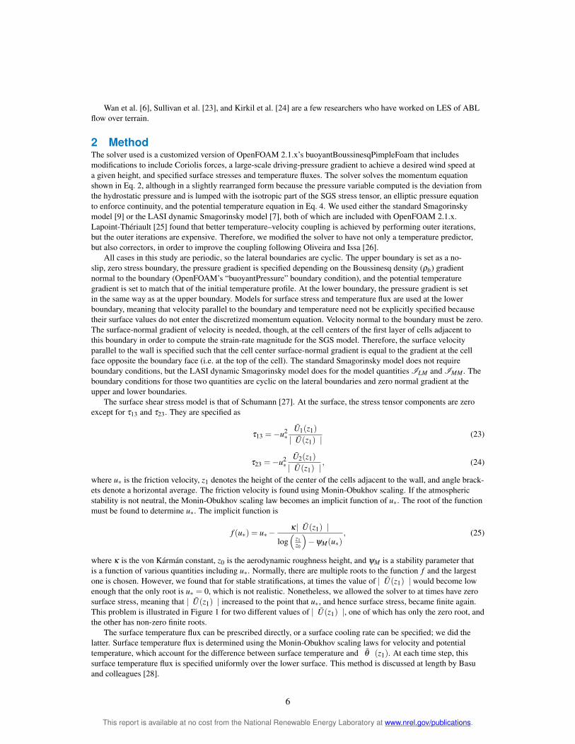
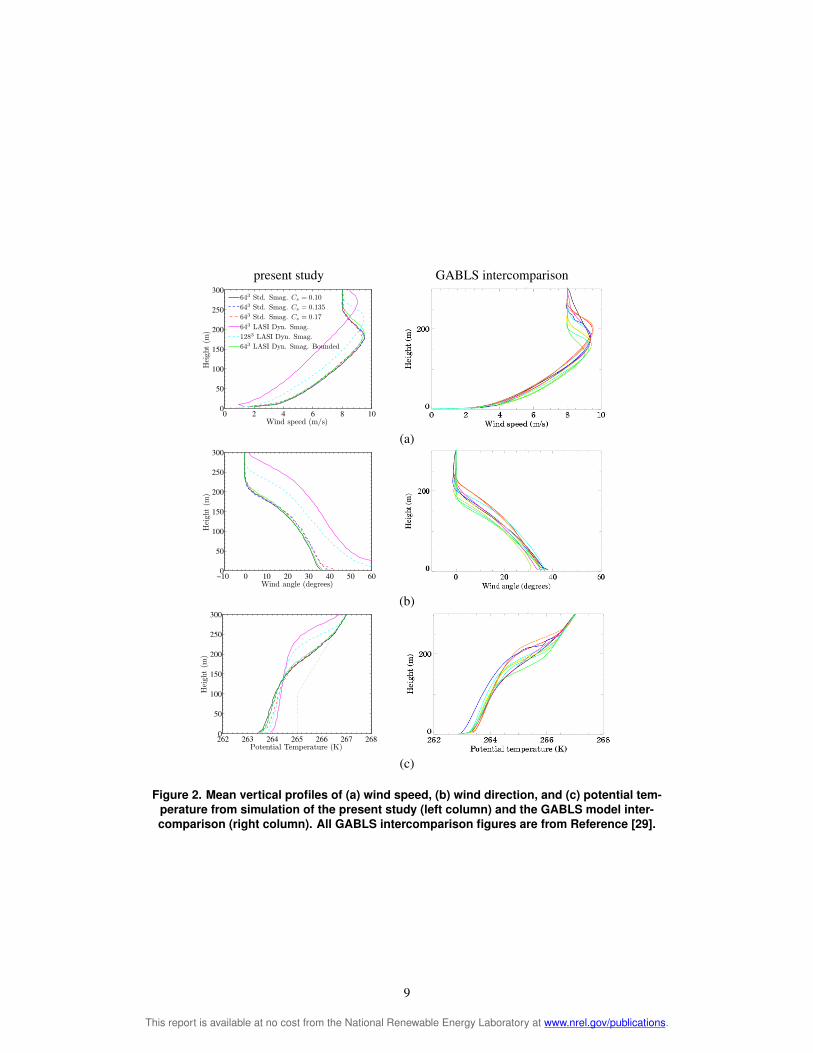
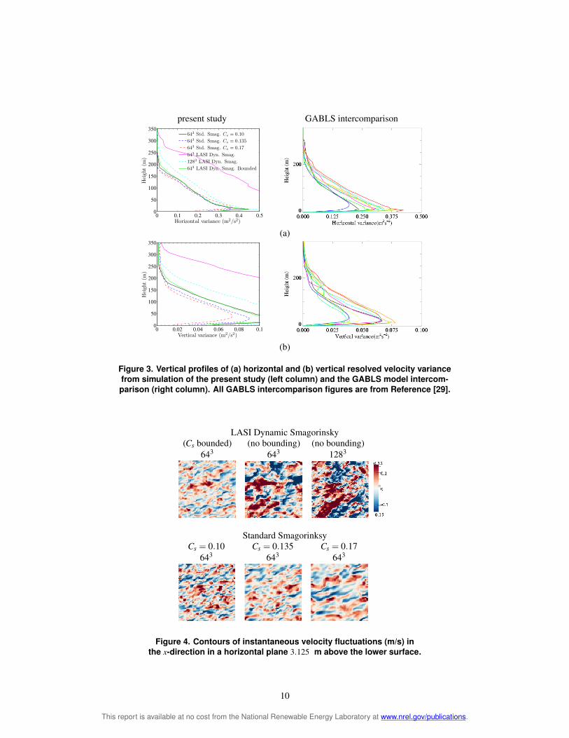
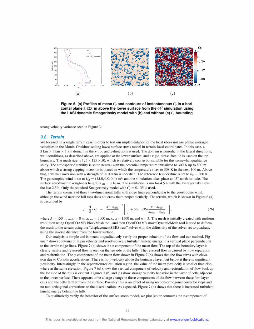
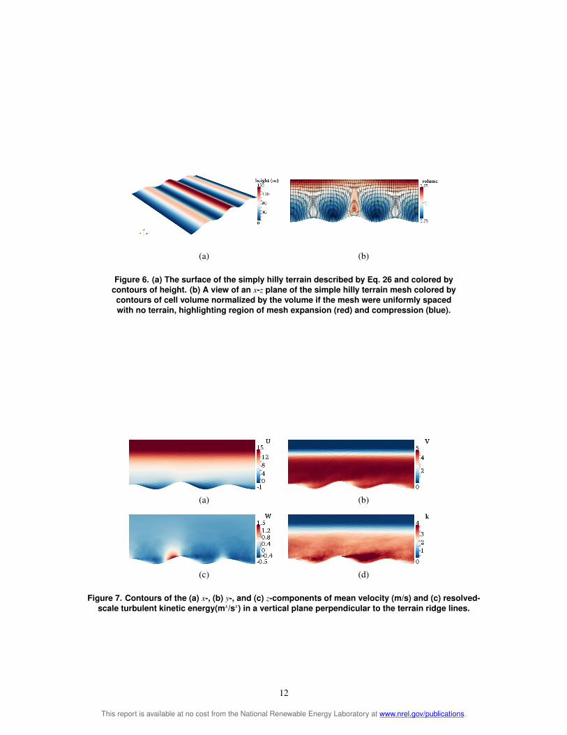
(a) (b)

Figure 6 (a) The surface of the simply hilly terrain described by Eq 26 and colored by

contours of height (b) A view of an x-z plane of the simple hilly terrain mesh colored by

contours of cell volume normalized by the volume if the mesh were uniformly spaced

with no terrain highlighting region of mesh expansion (red) and compression (blue)

(a) (b)

(c) (d)

Figure 7 Contours of the (a) x- (b) y- and (c) z-components of mean velocity (ms) and (c) resolved-

scale turbulent kinetic energy(msss) in a vertical plane perpendicular to the terrain ridge lines

12

This report is available at no cost from the National Renewable Energy Laboratory at wwwnrelgovpublications

Figure 8 Contours (colored) of the x-component of instantaneous velocshy

ity (ms) in cells adjacent to the hilly surface and the contour (black lines) of

where the x-directed component of instantaneous surface shear stress is zero

instantaneous velocity in the cells adjacent to the surface in Figure 8 We also plot (black line) the contour of where the x-directed component of the surface shear stress is zero Surface shear stress equal to zero can be an indicator of separated flow Figure 8 shows that the locations where the flow separates (where its velocity goes to zero and then reverses) are well correlated with the contour of zero shear stress

4 Conclusion and Future Work This document presents our initial work at adding the capability to NRELrsquos OpenFOAM-based SOWFA flow solver to simulate stably stratified atmospheric boundary layer flow and flow over complex terrain Before this work SOWFArsquos handling of the SGS terms in the momentum and potential temperature equations was not the same as in all other OpenFOAM solvers so it was not compatible with the SGS models that come standard with OpenFOAM We have migrated SOWFA back to the OpenFOAM-standard SGS treatment and can use models like the LASI dynamic Smagorinsky model Also before this work the surface stress and temperature flux models included with SOWFA were formulated in such a way that they were only compatible with flat terrain Now these models have the ability to work in terrain-local coordinates and the Monin-Obukhov scaling laws used by the models can be applied locally

We applied our new method to the stably stratified ABL GABLS model intercomparison test case using both the standard and LASI dynamic Smagorinsky models Surprisingly the standard Smagorinsky model which is often viewed as too dissipative for stably stratified flows in which turbulence levels are low andor intermittent produced mean vertical profiles of wind speed direction and potential temperature and variance profiles very similar to the simulation results of the GABLS intercomparison The LASI dynamic Smagorinsky results were much different That SGS model caused a much deeper boundary layer (roughly 300 m versus less than 200 m) and far greater peak velocity variances Contours of instantaneous velocity fluctuations show much stronger fluctuations in the LASI dynamic Smagorinsky cases as compared to the standard Smagorinsky cases We found that the model produces spikes of Cs with values as high as 46 so we applied bounding to the value of Cs If greater than 014 or less than 007 Cs is clipped The bounded LASI dynamic Smagorinksy results are much more in line with the GABLS participant results and the standard Smagorinksy results for Cs = 01 A possible next step is to implement one of the LASD dynamic Smagorinsky model variants which have been shown in the literature to produce better results than the LASI variant

In simulating the GABLS case in which surface temperature cooling rate is specified rather than surface temperature flux itself we found it difficult to obtain a meaningful friction velocity and surface temperature flux to create the desired cooling rate Specifically solving for the friction velocity and temperature flux requires finding the roots of a polynomial and normally the largest positive root is chosen for friction velocity Depending on the flow situation we found there to be many durations in the simulation in which the only solution was that friction velocity is zero which is unrealistic We need to remedy this problem in future work

Next we applied our new method to flow over an idealized hilly terrain under neutral atmospheric stratification This was only a qualitative study but it did confirm that the localized terrain-local surface stress formulation goes to zero and switches sign when moving into a region of flow separation More quantitative testing of our terrain methods is necessary and we plan to simulate cases for which experimental data are available such as the Askervein [30] and Bolund hills

We also plan to reexamine the use of local Monin-Obukhov scaling in the surface stress and temperature flux models Monin-Obukhov scaling was derived from average velocity temperature and moisture profiles so using

13

This report is available at no cost from the National Renewable Energy Laboratory at wwwnrelgovpublications

the scaling locally does not necessarily make sense The scaling laws were also derived for flow over relatively flat terrain We should not expect this scaling (ie the log-law) to hold over complex terrain Another option is to use detached-eddy simulation in which a Reynolds-averaged Navier-Stokes model handles the region near the surface that the surface stress and temperature flux models currently handle Yet one more option is to apply some sort of local terrain curvature correction to the standard scaling laws

Acknowledgments We would like to acknowledge Sukanta Basu and Yao Wang for their help and advice in simulating the stably stratified ABL We would like to thank David Lapoint-Theacuteriault for his useful ideas in implementing the surface stress model We also would like to thank Marshall Buhl Andy Platt Billy Hoffman and Rodd Hamann for their help with the computer resources used in this study This work was supported by the US Department of Energy under Contract No DE-AC36-08GO28308 with the National Renewable Energy Laboratory

14

This report is available at no cost from the National Renewable Energy Laboratory at wwwnrelgovpublications

Bibliography [1] M J Churchfield S Lee P J Moriarty Luis A Martiacutenez S Leonardi G Vijayakumar and J G Brasseur

A large-eddy simulation of wind-plant aerodynamics In 50th AIAA Aerospace Sciences Meeting including the New Horizons Forum and Aerospace Exposition Nashville TN Jan 9ndash12 2012 AIAA Washington DC 2012 AIAA Paper 2012-537

[2] A R Brown S H Derbyshire and P J Mason Large-eddy simulation of stable atmospheric boundary layers with a revised stochastic subgrid model Quarterly Journal of the Royal Meteorological Society 1201485ndash 1512 1994

[3] R J Beare M K MacVean A A M Holtslag J Cuxart I Esau J-C Golaz M A Jimenez M Khairoutshydinov B Kosovic D Lewellen T S Lund J K Lundquist A McCabe A F Moene Y Noh S Raasch and P Sullivan An intercomparison of large-eddy simulations of the stable boundary layer Boundary-Layer Meteorology 118247ndash272 2006

[4] R Stoll and F Porteacute-Agel Dynamic subgrid-scale models for momentum and scalar fluxes in large-eddy simulations of neutrally stratified atmospheric boundary layers over heterogeneous terrain Water Resources Research 42W01409 2006

[5] R Stoll and F Porteacute-Agel Large-eddy simulation of the stable atmospheric boundary layer using dynamic models with different averaging schemes Boundary-Layer Meteorology 1261ndash28 2008

[6] F Wan F Porteacute-Agel and R Stoll Evaluation of dynamic subgrid-scale models in large-eddy simulations of neutral turbulent flow over a two-dimensional sinusoidal hill Atmospheric Environment 41(13)2719ndash2728 2007

[7] C Meneveau T Lund and W Cabot A lagrangian dynamic subgrid-scale model of turbulence Journal of Fluid Mechanics 319353ndash385 1996

[8] N D Kelley Turbulence-turbine interaction The basis for the development of the TurbSim stochastic simulator Technical Report TP-5000-52353 National Renewable Energy Laboratory 2011

[9] J Smagorinksy General circulation experiments with the primitive equations Monthly Weather Review 9199ndash164 1963

[10] C-H Moeng A large-eddy simulation model for the study of planetary boundary layer turbulence Journal of the Atmospheric Sciences 41(13)2052ndash2062 July 1984

[11] P J Mason and S H Derbyshire Large-eddy simulation of the stably-stratified atmospheric boundary layer Boundary-Layer Meteorology 53117ndash162 1990

[12] P J Mason and D J Thompson Stochastic backscatter in large-eddy simulations of boundary layers Journal of Fluid Mechanics 24251ndash78 1992

[13] P P Sullivan J C McWilliams and C-H Moeng A subgrid-scale model for large-eddy simulation of planetary boundary-layer flows Boundary-Layer Meteorology 71247ndash276 1994

[14] A Andren The structure of the stably stratified atmospheric boundary layer A large-eddy simulation study Quarterly Journal of the Royal Meteorological Society 121(525)961ndash985 1995

[15] B Kosovic Subgrid-scale modelling for the large-eddy simulation of high-reynolds-number boundary layers Journal of Fluid Mechanics 336151ndash182 1997

[16] B Kosovic and J A Curry A large eddy simulation study of the quasi-steady stably stratified atmospheric boundary layer Journal of the Atmospheric Sciences 571052ndash1068 2000

[17] M Germano U Piomelli P Moin and W Cabot A dynamic subgrid-scale eddy viscosity model Physics of Fluids A 31760ndash1765 1991

15

This report is available at no cost from the National Renewable Energy Laboratory at wwwnrelgovpublications

[18] F Porteacute-Agel C Meneveau and M B Parlange A scale-dependent dynamic model for large-eddy simshyulation Application to a neutral atmospheric boundary layer Journal of Fluid Mechanics 415261ndash284 2000

[19] E Bou-Zeid C Meneveau and M Parlange A scale-dependent lagrangian dynamic model for large-eddy simulation of complex turbulent flows Physics of Fluids 17025105 2005

[20] S Basu and F Porteacute-Agel Large-eddy simulation of stably stratified atmospheric boundary layer turbulence A scale-dependent dynamic modeling approach Journal of the Atmospheric Sciences 632074ndash2091 2006

[21] R J Beare and M K MacVean Resolution sensitivity and scaling of large-eddy simulations of the stable boundary layer Boundary-Layer Meteorology 112257ndash281 2004

[22] J Kleissl V Kumar C Meneveau and M B Parlange Numerical study of dynamic smagorinsky models in large-eddy simulation of the atmospheric boundary layer Validation in stable and unstable conditions Water Resources Research 442W06D10 2006

[23] P P Sullivan E G Patton and K W Ayotte Turbulent flow over and around sinusoidal bumps hills gaps and craters derived from large eddy simulations In 19th Conference on Boundary Layer and Turbulence Keystone CO Aug 2ndash6 2010 2010 Paper 1B5

[24] G Kirkil J Mirocha E Bou-Zeid F K Chow and B Kosovic Implementation and evaluation of dynamic subfilter scale stress models for large eddy simulation using WRF Monthly Weather Review 140266ndash284 2012

[25] David Lapoint-Theacuteriault Vers Une Reacutesolution Numeacuterique du Vent Dans la Couche Limite Atmospheacuterique agrave Micro-eacutechelle Ave La Meacutethode de Simulation des Grandes eacutechelles (LES) Sous OpenFOAM PhD thesis Eacutecole De Technologie Supeacuterieure 2012

[26] P J Oliveira and R I Issa An improved PISO algorithm for the computation of buoyancy-driven flows Numerical Heat Transfer Part B 40473ndash493 2001

[27] U Schumann Subgrid scale model for finite difference simulations of turbulent flows in plane channels and annuli Journal of Computational Physics 18376ndash404 1975

[28] S Basu A A M Holtslag B J H Van De Weil A F Moene and G-J Steeneveld An inconvenient ldquotruthrdquo about using sensible heat flux as a surface boundary condition in models under stably stratified regimes Acta Geophysica 56(1)88ndash99 2008

[29] GABLS LES intercomparison httpgablsmetofficecomindexhtml 2006

[30] P A Taylor and H W Teunissen The askervein hill project Report on the SeptOct 1983 main field experiment Technical Report Report Number MSRBndash84ndash6 Research Canada 1985 Available online at httpwwwyorkucapatresearchAskerveinindexhtml

16

This report is available at no cost from the National Renewable Energy Laboratory at wwwnrelgovpublications
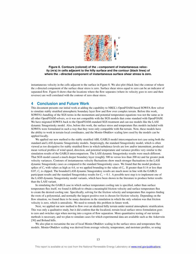