Addressing the Multiplicity of Solutions in Optical Lens Designas a Niching Evolutionary Algorithms Computational Challenge

Anna V. KononovaLIACS, Leiden University

The Netherlandsa.kononova@liacs.leidenuniv.nl

Ofer M. ShirComputer Science Department,

Tel-Hai College, and Migal InstituteUpper Galilee, Israelofersh@telhai.ac.il

Teus TukkerASML

Veldhoven, The Netherlandsteus.tukker@asml.com

Pierluigi FriscoASML

Veldhoven, The Netherlands

Shutong ZengLIACS, Leiden University

The Netherlands

Thomas BäckLIACS, Leiden University

The Netherlands

ABSTRACTOptimal Lens Design constitutes a fundamental, long-standing real-world optimization challenge. Potentially large number of optima,rich variety of critical points, as well as solid understanding ofcertain optimal designs per simple problem instances, provide al-together the motivation to address it as a niching challenge. Thisstudy applies established Niching-CMA-ES heuristic to tackle thisdesign problem (6-dimensional Cooke triplet) in a simulation-basedfashion. The outcome of employing Niching-CMA-ES ‘out-of-the-box’ proves successful, and yet it performs best when assisted bya local searcher which accurately drives the search into optima.The obtained search-points are corroborated based upon concreteknowledge of this problem-instance, accompanied by gradient andHessian calculations for validation. We extensively report on thiscomputational campaign, which overall resulted in (i) the locationof 19 out of 21 known minima within a single run, (ii) the discov-ery of 540 new optima. These are new minima similar in shapeto 21 theoretical solutions, but some of them have better meritfunction value (unknown heretofore), (iii) the identification of nu-merous infeasibility pockets throughout the domain (also unknownheretofore). We conclude that niching mechanism is well-suitedto address this problem domain, and hypothesize on the apparentmultidimensional structures formed by the attained new solutions.

CCS CONCEPTS•Computingmethodologies→Model development and anal-ysis; Artificial intelligence; • Applied computing; • Theory ofcomputation→ Continuous optimization;

KEYWORDSLens design, niching, continuous optimization, Cooke triplet

Permission to make digital or hard copies of part or all of this work for personal orclassroom use is granted without fee provided that copies are not made or distributedfor profit or commercial advantage and that copies bear this notice and the full citationon the first page. Copyrights for third-party components of this work must be honored.For all other uses, contact the owner/author(s).Preprint, arXiv, 2021© 2021 Copyright held by the owner/author(s).

1 INTRODUCTIONThe domain of Optical Lens Design [7] offers a variety of highlycomplex optimization problem instances: the solution spaces arevery rugged, and the extensive mathematical techniques are oflimited use in most of the cases. The conventional approach fol-lowed in designing lenses is to create a few designs using one’sown experience, then let commercial packages (e.g., Code V [4] andOpicStudio [19]) to optimize these designs using gradient-basedlocal search. Different techniques have been used to determine lensdesigns. For example, [26] gives an overview of classical and Evo-lutionary Algorithms (EAs) for the optimization of optical systems,[12] compares different global optimization algorithms on freeformoptical designs, [11] reviews the use of genetic algorithms for lensdesign, and different mathematical techniques are employed tolocate the minima of specific lens designs in [2, 25].

Generally speaking, most of the approaches aim to locate theglobal optima, whereas only a few are designed to find local op-tima (see, e.g., [25]). As mentioned earlier, because many factors(manufacturability, cost, etc,) are unknown a-priori, and have thepotential to influence the choice of the final design, it makes senseto come up with methodologies searching for as many local optimaas possible having some key performance indicator (KPI) valuesbelow/above given thresholds1.

In this study we propose a novel approach for the challenge oflocating as many local minima as possible in the domain of opticallens system designs (i.e., optical systems). Our proposed approachis based on the application of a niching algorithm that relies on avariant of the Covariance Matrix Adaptation Evolution Strategy(CMA-ES) [23], combined with local search.

Lens designs are subject to input and output constraints: thetype of light the optical system has to deal with, the magnifica-tion/reduction factor the optical system must achieve, the focallength the optical system must have, the occupied volume and man-ufacturability tolerances, and the maximum cost of the system. TheKPIs of a lens design can be many and they are related to aber-rations, i.e., imperfections in image formation. These aberrations1The so-called Second Toyota Paradox, which is often reviewed in management studies,promotes the consideration of multiple candidate solutions during the car productionprocess [5]:

"Delaying decisions, communicating ambiguously, and pursuing anexcessive number of prototypes, can produce better cars faster andcheaper."

arX

iv:2

105.

1054

1v1

[cs

.CE

] 2

1 M

ay 2

021

Preprint, arXiv, 2021 Kononova et al.

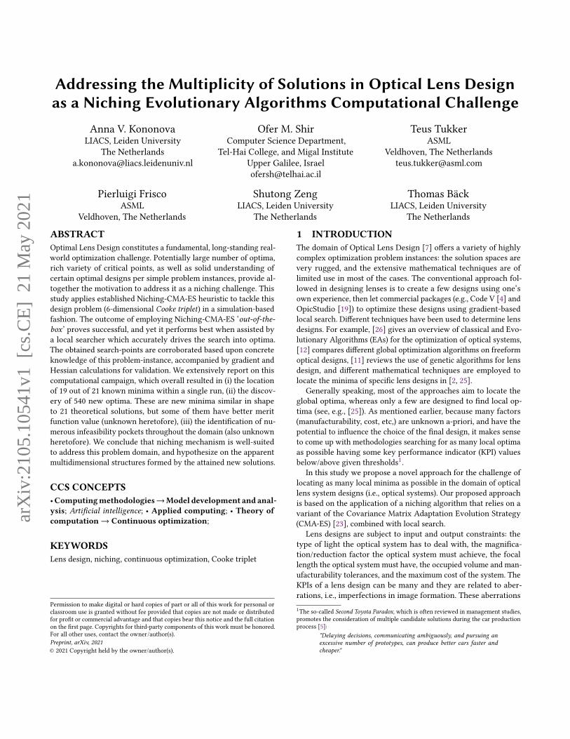
Figure 1: Depiction of a simple lens designwhere the centralray hits the center of the focal plane and an off-center rayhits the focal plane with a displacement from the desiredcenter position.

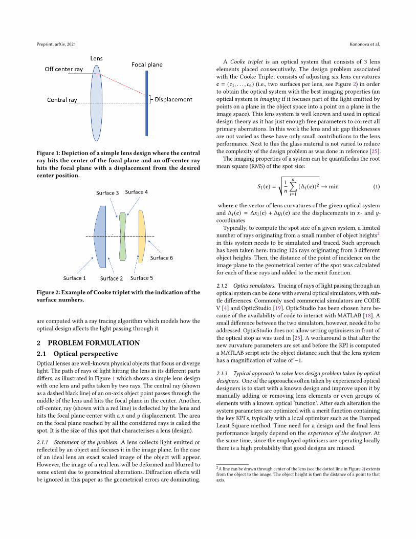
Figure 2: Example of Cooke triplet with the indication of thesurface numbers.

are computed with a ray tracing algorithm which models how theoptical design affects the light passing through it.

2 PROBLEM FORMULATION2.1 Optical perspectiveOptical lenses are well-known physical objects that focus or divergelight. The path of rays of light hitting the lens in its different partsdiffers, as illustrated in Figure 1 which shows a simple lens designwith one lens and paths taken by two rays. The central ray (shownas a dashed black line) of an on-axis object point passes through themiddle of the lens and hits the focal plane in the center. Another,off-center, ray (shown with a red line) is deflected by the lens andhits the focal plane center with a 𝑥 and 𝑦 displacement. The areaon the focal plane reached by all the considered rays is called thespot. It is the size of this spot that characterises a lens (design).

2.1.1 Statement of the problem. A lens collects light emitted orreflected by an object and focuses it in the image plane. In the caseof an ideal lens an exact scaled image of the object will appear.However, the image of a real lens will be deformed and blurred tosome extent due to geometrical aberrations. Diffraction effects willbe ignored in this paper as the geometrical errors are dominating.

A Cooke triplet is an optical system that consists of 3 lenselements placed consecutively. The design problem associatedwith the Cooke Triplet consists of adjusting six lens curvaturesc = (𝑐1, . . . , 𝑐6) (i.e., two surfaces per lens, see Figure 2) in orderto obtain the optical system with the best imaging properties (anoptical system is imaging if it focuses part of the light emitted bypoints on a plane in the object space into a point on a plane in theimage space). This lens system is well known and used in opticaldesign theory as it has just enough free parameters to correct allprimary aberrations. In this work the lens and air gap thicknessesare not varied as these have only small contributions to the lensperformance. Next to this the glass material is not varied to reducethe complexity of the design problem as was done in reference [25].

The imaging properties of a system can be quantifiedas the rootmean square (RMS) of the spot size:

𝑆1 (c) =

√√1𝑛

𝑛∑︁𝑖=1(Δ𝑖 (c))2 → min (1)

where c the vector of lens curvatures of the given optical systemand Δ𝑖 (c) = Δ𝑥𝑖 (c) + Δ𝑦𝑖 (c) are the displacements in 𝑥- and 𝑦-coordinates

Typically, to compute the spot size of a given system, a limitednumber of rays originating from a small number of object heights2in this system needs to be simulated and traced. Such approachhas been taken here: tracing 126 rays originating from 3 differentobject heights. Then, the distance of the point of incidence on theimage plane to the geometrical center of the spot was calculatedfor each of these rays and added to the merit function.

2.1.2 Optics simulators. Tracing of rays of light passing through anoptical system can be done with several optical simulators, with sub-tle differences. Commonly used commercial simulators are CODEV [4] and OpticStudio [19]. OpticStudio has been chosen here be-cause of the availability of code to interact with MATLAB [18]. Asmall difference between the two simulators, however, needed to beaddressed. OpticStudio does not allow setting optimisers in front ofthe optical stop as was used in [25]. A workaround is that after thenew curvature parameters are set and before the KPI is computeda MATLAB script sets the object distance such that the lens systemhas a magnification of value of −1.

2.1.3 Typical approach to solve lens design problem taken by opticaldesigners. One of the approaches often taken by experienced opticaldesigners is to start with a known design and improve upon it bymanually adding or removing lens elements or even groups ofelements with a known optical ‘function’. After each alteration thesystem parameters are optimized with a merit function containingthe key KPI’s, typically with a local optimizer such as the DampedLeast Square method. Time need for a design and the final lensperformance largely depend on the experience of the designer. Atthe same time, since the employed optimisers are operating locallythere is a high probability that good designs are missed.

2A line can be drawn through center of the lens (see the dotted line in Figure 2) extentsfrom the object to the image. The object height is then the distance of a point to thataxis.

Addressing the Multiplicity of Solutions in Optical Lens Design as a Niching Evolutionary Algorithms Computational Challenge Preprint, arXiv, 2021

Therefore, strictly speaking, no directly competitive computationalapproaches exist in the field of optics for the methodology proposedin this paper.

2.1.4 Infeasible lens designs. Clearly, some lens designs can re-sult in rays falling outside the focal plane or reflecting internally.For such designs, ray tracing simulators return a predefined largenumerical value.

2.2 Computational perspectiveThe lens design problem described in the previous section con-stitutes a (reasonably) low-dimensional continuous problem setwithin a simple hypercube domain whose objective function3 𝑓 (c)is based on a number of outputs obtained from an optics simulator4𝑆 :

𝑓 (c) = 𝑤1𝑆1 (𝒄) (2)+𝑤2 (𝑆EFFL (𝒄) − EFFLtarget)2

+𝑤3 (𝑆PMAG (𝒄) − PMAGtarget)2 → min ,

where c = (𝑐1, . . . , 𝑐6) ∈ [−0.25, 0.25]6 are lens curvatures,𝑆1 (𝒄) is the spot size merit function component defined in Sec-tion 2.1.1, 𝑆EFFL (𝒄) is the effective focal length component, and𝑆PMAG (𝒄) is the paraxial magnification, all three being computedby the simulator 𝑆 . The target values of the latter two are set asEFFLtarget = 30[mm] and PMAGtarget = −1, respectively, and theweights are chosen as 𝑤𝑖 = 1. Minimisation problem specified ineq. (2) is solved in this paper.

2.2.1 Analysis of known optima. The Cooke triplet lens designproblem has been intensively studied in the past. To date, the mostdetailed analysis of the problem [25] yields curvature values whichrepresent 21 locally optimal designs. This analysis is a mixtureof numerical simulation and physics-based theoretical reasoningabout the properties of a simplified objective function. The authorssuggest a methodology of constructing triplet minima from knownduplet minima (and, potentially for higher orders, incrementally)and build a classification of locally optimal designs according totheir morphology.

Their results, however, do not exclude the possibility of existenceof other local optima. The approach taken in this paper is to studyhow close a specialised evolutionary algorithm can get to the knownoptima in a purely numerical fashion, without utilizing any opticsknowledge.

2.2.2 Discrepancies between simulators. It should be mentionedthat results in [25] have been obtained using the Code V simulator.Meanwhile, in this study the OpticsStudio simulator has been em-ployed. To assure the compatibility of the two simulators, a studyhas been carried out where 21 known optima have been evaluatedin both simulators - results coincide up to the 5th decimal digit.

2.2.3 Nature of Critical Points. As described above, previous inves-tigation of this optimization domain, and particularly of this tripletproblem-instance, concluded that the underlying search landscapepossesses a rich variety of critical points [25]. Since we study the

3Referred to as KPI in the previous sections4The objective function used here is the same as in [25].

application of randomized search heuristics in a black-box fash-ion, an assessment of the attained solution-points is much neededin order to validate their nature as optima. To this end, we con-sider finite-differences calculations of the gradient vector and theHessian matrix [20], relying on the short evaluation times of thesimulator’s objective function calls. Explicitly, a critical point ofan objective function 𝑓 is where its gradient vector vanishes, i.e.,(∇𝑓 )𝑖 := 𝜕𝑓

𝜕𝑥𝑖= 0 ∀𝑖 . The Hessian of 𝑓 ,

(H𝑓

)𝑖 𝑗

:= 𝜕2 𝑓𝜕𝑥𝑖𝜕𝑥 𝑗

may

provide the diagnosis of the critical points by examination of itseigenvalues (which are guaranteed to be real due to its symmetry):a positive (negative) spectrum indicates a minimum (maximum),whereas a spectrum with mixed signs indicates a saddle point; theexistence of a zero eigenvalue suggests flatness and may requirehigher-order derivatives for assessment.

In practice, gradients and Hessian spectra of the 21 knowntheoretical solutions were approximated using finite-differences’calculations, and by utilizing a variety of infinitesimal pertur-bation values (delta steps) to validate the approximation (𝛿𝑥 :=10−4, 10−5, . . . , 10−12). The obtained gradients indeed reflect thecritical point nature of these solutions. Furthermore, we analyzedthe attained Hessian spectra. Evidently, the majority of the eigen-values vanish — indicating some flatness, but formally suggestinglack of conclusive statements. All spectra are dominated by a singledirection – which has been corroborated as a meaningful design bythe human experts – exhibiting high condition numbers at thesebasins of attraction. Notably, two optima appear to be saddle points(i.e., possess negative eigenvalues). This odd observation may beexplained by the discrepancies between the two simulators, sug-gesting that these critical-points’ locations (verified on Code-V)undergo a shift on OpticStudio.

2.2.4 Known Optima Locations. As amply demonstrated in thefield of computational intelligence [3, 6, 13–15], location of optimawithin the domain can influence the performance of heuristic opti-misation algorithms. Therefore, here we investigate how 21 knownoptima [25] are distributed within the problem domain and lookfor additional insights into the structure of the problem.

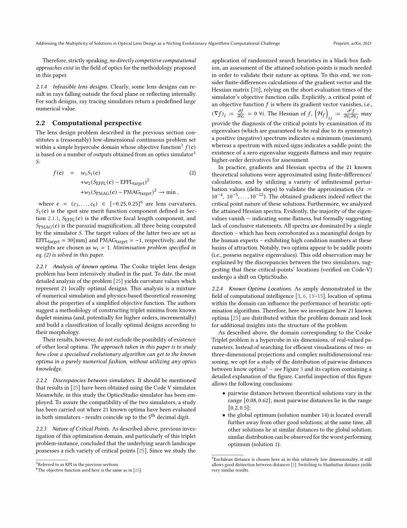
As described above, the domain corresponding to the CookeTriplet problem is a hypercube in six dimensions, of real-valued pa-rameters. Instead of searching for efficient visualisations of two- orthree-dimensional projections and complex multidimensional rea-soning, we opt for a study of the distribution of pairwise distancesbetween know optima5 – see Figure 3 and its caption containing adetailed explanation of the figure. Careful inspection of this figureallows the following conclusions:• pairwise distances between theoretical solutions vary in therange [0.08, 0.62]; most pairwise distances lie in the range[0.2, 0.5];• the global optimum (solution number 14) is located overallfurther away from other good solutions; at the same time, allother solutions lie at similar distances to the global solution;similar distribution can be observed for the worst performingoptimum (solution 1);

5Euclidean distance is chosen here as in this relatively low dimensionality, it stillallows good distinction between distances [1]. Switching to Manhattan distance yieldsvery similar results.

Preprint, arXiv, 2021 Kononova et al.

0.1

0.2

0.3

0.4

0.5

0.6

2 4 6 8 10 12 14 16 18 20

0.0025

0.003

0.0035

0.004

0.0045

0.005

0.0055

0.006

0.0065

0.007

0.0075

0.008

pa

irw

ise

Eu

clid

ea

n d

ista

nce

(th

is,

20

oth

er

the

ore

tica

l so

lutio

ns)

ob

jective

fu

nctio

n v

alu

etheoretical solution number

1

2

3

4

5

nu

mb

er

of

tim

es s

olu

tio

n h

as b

ee

n f

ou

nd

in

5 in

de

pe

nd

en

t ru

ns

Figure 3: Distribution of pairwise Euclidean distancesamong the known 21 theoretical solutions (6-dimensionalreal-valued decision vectors that are associated with 6 lenscurvatures), as identified in [25], having the solutions’ num-bering preserved. Orange dashes indicate the distribution ofall 21×20

2 pairwise distances among 21 theoretical solutions,i.e. they are projections of all rhombi onto the left verticalaxis. The objective function value of each theoretical solu-tion is depicted as a black circle, with values marked on theright vertical axis. Solution number 14 is the global min-imum. The rhombi symbols are colored according to thenumber of times a theoretical solution has been preciselylocated in a series of 5 independent runs of the final config-uration of the proposed method shown in Algorithm 1.

• other better solutions (17, 12, 9, 10) are also located furtheraway from other remaining solutions;• no direct correlation between the distribution of distances forsimilar performing solutions can be observed (e.g., solutions5 vs 18 or 6 vs 16);• in a series of 5 independent runs of the final configurationof the proposed method discussed in Section 3:★ all solutions have been found at least once; in total, 18 to

19 out of 21 solutions have been found in every single run;★ the least found solution (solution 18, found 1 time out of

5) is located further away from all other solutions;★ the second least found solution (solution 11, found 2 times

out of 5) is not drastically different from other solutions.

3 METHODOLOGY AND SETUPIn this section we elaborate on the computational approach taken,the preliminary planning, and the experimentation setup. We firstpresent the background of nichingmethods and specify the concretemethodology that we employ in this research.

3.1 Niching CMA-ESStandard Evolutionary Algorithms (EAs) tend to lose their popu-lation diversity and converge into a single solution [21]. Nichingmethods constitute the extension of EAs to finding multiple optima

in relevant search-landscapes within one population [21]. Theyaddress this issue by maintaining the diversity of certain propertieswithin the population, and thereby aim at obtaining parallel con-vergence into multiple basins of attraction in the landscape withina single run. Research on niching methods started in Genetic Algo-rithms [17], followed by work in Evolution Strategies [23, 24], andbroadened to the entire field of nature-inspired heuristics yieldingaltogether a sheer volume of potent techniques (see [16] for a recentreview).

Here, given the optimization problem at hand, we choose toemploy the established, radius-based Niching CMA-ES technique[23] using a (1, _) kernel. The targeted number of niches is denotedby 𝑞. In short, following the evaluation of the population, niches arespatially constructed around peak individuals, in a greedy manner,based upon the prescribed niche radius 𝜌 . Resources are uniformlypartitioned per niche, thus each peak individual is sampled _ timesin the following generation6.

3.2 Parameter SettingsWe employ the niching within a (1, _)-CMA-ES algorithm, andspecify in what follows its parameters’ settings by adhering to thenotation in [23]. We target 𝑞 = 20 niches per each run, yet allocatefurther 𝑝 = 5 dynamic peaks (i.e., 25 D-sets are formed). Regardingpopulation sizing, we follow the recommendation and set _ = 10 –yielding altogether 250 individuals that undergo evaluation in eachiteration. Importantly, setting the niche radius value may have acritical impact on the behavior of a niching routine that features afixed radius, often referred to as the niche radius problem [24]. Here,rather than approximating the search volume and partitioning itamong the niches [24], we are in a position to capitalize on theknown theoretical solutions. We assume that their spatial distri-bution is indicative of the general distribution of solution pointswithin the feasible space, and set accordingly the niche radius tohalf of the mean pairwise distances (see Figure 3): 𝜌 = 0.18. Oth-erwise, the cycle of non-peak reset is set to ^ = 20 iterations, andthe initial global step-size is set to 𝜎0 = 0.05. Solutions generatedoutside the domain are corrected by placing them on the boundary[13].

3.3 Local Search UtilizationThe so-called Dampened Least Squares (DLS) [9, 26] (also knownas the Levenberg-Marquardt algorithm) constitutes a modificationof the well-known Newton-Raphson method [20]. It is traditionallyemployed in lens design, and it became a built-in option in theOpticsStudio simulator. This local search method on its own, beingdependent upon ‘good’ initial points, is unlikely to locate all theoptima of the problem. We thus utilised it for validation purposes,as explained in Section 2.2.3. At the same time, preliminary experi-ments suggested that minor improvements are often achieved whenthis local searchmethod is applied to the solution-points attained bythe niching algorithm, regardless of the niching configuration andits parameters’ setting. We explain these observed improvements

6In socio-biological terms, the peak individual is associated with an alpha-male,which wins the local competition and gets all the sexual resources of its ecologicalniche. The algorithm as a whole can be thus considered as a competition between alpha-males, each of which is fighting for one of the available 𝑞 “computational resources”,after winning its local competition at the “ecological optimum” site.

Addressing the Multiplicity of Solutions in Optical Lens Design as a Niching Evolutionary Algorithms Computational Challenge Preprint, arXiv, 2021

by the landscape’s rich variety of critical points, including saddlepoints, which seemingly render the convergence attempts by theCMA-ES challenging. We therefore devised a hybrid approach, asoutlined in Algorithm 1.

Algorithm 1 The Proposed Niching-(1, _)-CMA-ES + DLS HybridApproach1: 𝑖 ← 12: 𝑎 ← ∅ ⊲ initialise solution archive3: 𝑜 ← ∅ ⊲ initialise optima archive4: 𝑑 ← 10 ⊲ set archive search depth5: 𝑝 [𝑖] ← initialise niching (1, _)-CMA-ES ⊲ see Section 3.26: while fitness evaluation budget permits do7: 𝑝 [𝑖 + 1] ← 𝑖𝑡ℎ generation of niching (1, _)-CMA-ES ⊲ [23]8: 𝑎[𝑖] ← 𝑝 [𝑖] ⊲ update solution archive9: 𝑖 ← 𝑖 + 110: end while11: for 𝑗 = 𝑖 − 𝑑 → 𝑖 − 1 do ⊲ take last 𝑑 generations12: while 𝑎[ 𝑗] is not empty do13: 𝑠 ← fetch next element of 𝑎[ 𝑗]14: 𝑜 ← 𝑜 ∪ 𝐷𝐿𝑆 (𝑠) ⊲ via OpticsStudio715: end while16: end for17: return filter(𝑜) ⊲ remove duplicates, return optima archive

3.4 Setup and Experimental PlanningOur niching implementation follows the publicly available sourcecode [22]. The niching algorithm was run using the configurationfrom Section 3.2 for up to 25000 objective function evaluations,with the variation operator being adjusted within the predefined6-dimensional boundaries. An approximate duration of a singleobjective function call is within the range of 2 sec. All the experi-ments were run using MATLAB and executed on Windows Intel(R)Core(R)i5 CPU 8350 @ 1.90GHz with 4 processing units. The fi-nal Niching-(1, _)-CMA-ES configuration has been run 5 times,meanwhile overall, we conducted 60 runs with various settings.

4 RESULTS AND ANALYSESOur proposed approach located altogether 540 optima within thisdomain. Furthermore, during the reported experimentation, all theevaluated candidate solution-points (i.e., lens designs) visited bythe aforementioned approach have been recorded. Upon filteringout duplicate points, 185200 unique feasible candidate solution-points were altogether located, versus 245880 infeasible candidatesolution-points. Next, we elaborate on these observations and offerinsights into the landscape.

4.1 Distribution of Known and Novel OptimaThe aforementioned experimentation has consistently indicatedthe existence of new locally optimal solutions. Overall, 540 newsolutions have been identified and further investigated for local

7Apply DLS implementation from OpticStudio until the internal termination criteriais not hit: no significant improvement in the value of the objective function.

0

0.1

0.2

0.3

0.4

0.5

0.6

0.7

2 4 6 8 10 12 14 16 18 20

0.0025

0.003

0.0035

0.004

0.0045

0.005

0.0055

0.006

0.0065

0.007

0.0075

0.008

pa

irw

ise

Eu

clid

ea

n d

ista

nce

(th

is t

he

ore

tica

l, 5

40

ne

w s

olu

tio

ns)

fitn

ess v

alu

e o

f th

is t

he

ore

tica

l so

lutio

n

theoretical solution number

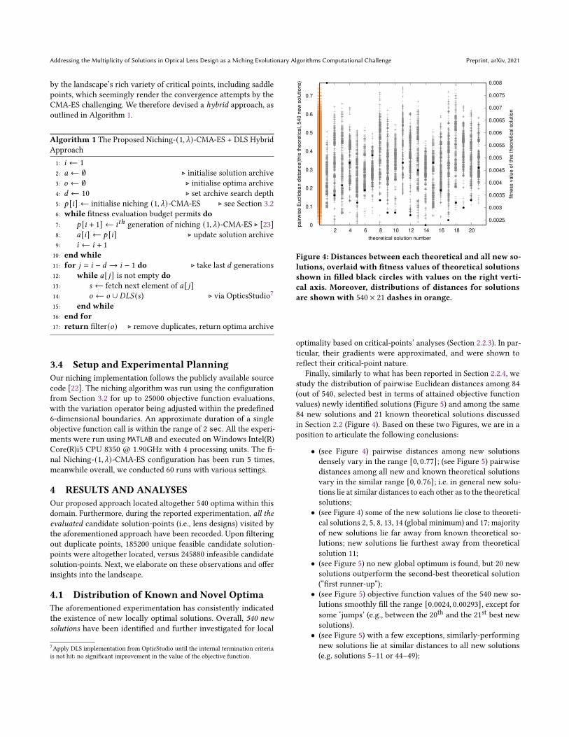
Figure 4: Distances between each theoretical and all new so-lutions, overlaid with fitness values of theoretical solutionsshown in filled black circles with values on the right verti-cal axis. Moreover, distributions of distances for solutionsare shown with 540 × 21 dashes in orange.

optimality based on critical-points’ analyses (Section 2.2.3). In par-ticular, their gradients were approximated, and were shown toreflect their critical-point nature.

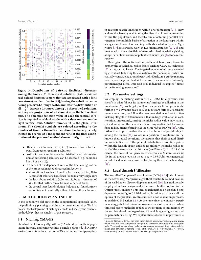
Finally, similarly to what has been reported in Section 2.2.4, westudy the distribution of pairwise Euclidean distances among 84(out of 540, selected best in terms of attained objective functionvalues) newly identified solutions (Figure 5) and among the same84 new solutions and 21 known theoretical solutions discussedin Section 2.2 (Figure 4). Based on these two Figures, we are in aposition to articulate the following conclusions:

• (see Figure 4) pairwise distances among new solutionsdensely vary in the range [0, 0.77]; (see Figure 5) pairwisedistances among all new and known theoretical solutionsvary in the similar range [0, 0.76]; i.e. in general new solu-tions lie at similar distances to each other as to the theoreticalsolutions;• (see Figure 4) some of the new solutions lie close to theoreti-cal solutions 2, 5, 8, 13, 14 (global minimum) and 17; majorityof new solutions lie far away from known theoretical so-lutions; new solutions lie furthest away from theoreticalsolution 11;• (see Figure 5) no new global optimum is found, but 20 newsolutions outperform the second-best theoretical solution(“first runner-up”);• (see Figure 5) objective function values of the 540 new so-lutions smoothly fill the range [0.0024, 0.00293], except forsome ‘jumps’ (e.g., between the 20th and the 21st best newsolutions).• (see Figure 5) with a few exceptions, similarly-performingnew solutions lie at similar distances to all new solutions(e.g. solutions 5–11 or 44–49);

Preprint, arXiv, 2021 Kononova et al.

0

0.1

0.2

0.3

0.4

0.5

0.6

0.7

4 8 12 16 20 24 28 32 36 40 44 48 52 56 60 64 68 72 76 80 84 0.0023

0.0024

0.0025

0.0026

0.0027

0.0028

0.0029

pa

irw

ise

Eu

clid

ea

n d

ista

nce

(th

is n

ew

, a

ll o

the

r n

ew

so

lutio

ns)

fitn

ess v

alu

e o

f th

is n

ew

so

lutio

n

new solution number

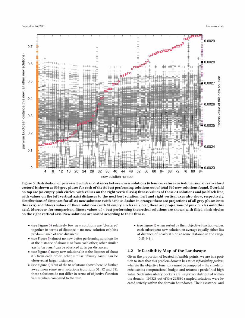
Figure 5: Distribution of pairwise Euclidean distances between new solutions (6 lens curvatures or 6-dimensional real-valuedvectors) is shown as 539 grey pluses for each of the 84 best performing solutions out of total 540 new solutions found. Overlaidon top are (as empty pink circles, with values on the right vertical axis) fitness values of these 84 solutions and (as black line,with values on the left vertical axis) distances to the next best solution. Left and right vertical axes also show, respectively,distributions of distances for all 84 new solutions (with 539 × 84 dashes in orange; these are projections of all grey pluses ontothis axis) and fitness values of these solutions (with 84 empty circles in violet; these are projections of pink circles onto thisaxis). Moreover, for comparison, fitness values of 4 best performing theoretical solutions are shown with filled black circleson the right vertical axis. New solutions are sorted according to their fitness.

• (see Figure 5) relatively few new solutions are ‘clustered’together in terms of distance – no new solution exhibitspredominance of zero distances;• (see Figure 5) almost no new better performing solutions lieat the distance of about 0.12 from each other; other similar‘exclusion zones’ can be observed at larger distances;• (see Figure 5) many new solutions lie at the distance of about0.3 from each other; other similar ‘density zones’ can beobserved at larger distances;• (see Figure 5) 3 out of the 84 solutions shown here lie furtheraway from some new solutions (solutions 31, 52 and 78);these solutions do not differ in terms of objective functionvalues when compared to the rest;

• (see Figure 5) when sorted by their objective function values,each subsequent new solution on average equally either liesat distance of nearly 0.0 or at some distance in the range[0.25, 0.4];

4.2 Infeasibility Map of the LandscapeGiven the proportion of located infeasible points, we are in a posi-tion to state that this problem domain has inner infeasibility pockets,wherein the objective function cannot be computed – the simulatorexhausts its computational budget and returns a predefined highvalue. Such infeasibility pockets are uniformly distributed withinthe domain: 109328 out of the 245880 sampled solutions were lo-cated strictly within the domain boundaries. Their existence, and

Addressing the Multiplicity of Solutions in Optical Lens Design as a Niching Evolutionary Algorithms Computational Challenge Preprint, arXiv, 2021

245880 sampled solutions

109328 infeasible inside domain ≈ 6 × 109 p/w distances

500 subsampled infeasible |100𝑖=1

1𝑠𝑡min|100𝑖=1

... 10𝑡ℎmin|100𝑖=1

≈ 1.2 × 105 p/w distances |100𝑖=1

5000 subsamples |100𝑖=1

Shapiro-Wilk p-values |100𝑖=1Figure 7

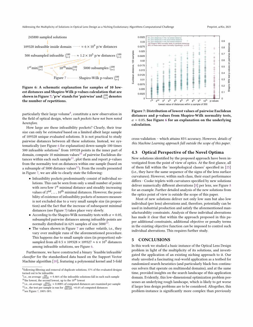
Figure 6: A schematic explanation for samples of 10 low-est distances and Shapiro-Wilk p-values calculation that areshown in Figure 7; ‘p/w’ stands for ‘pairwise’ and |100

𝑖=1 denotesthe number of repetitions.

particularly their large volume8, constitute a new observation inthe field of optical design, where such pockets have not been notedheretofore.

How large are these infeasibility pockets? Clearly, their truesize can only be estimated based on a limited albeit large sampleof 109328 unique evaluated solutions. It is not practical to studypairwise distances between all these solutions. Instead, we sys-tematically (see Figure 6 for explanation) down-sample 100 times500 infeasible solutions9 from 109328 points in the inner part ofdomain, compute 10 minimum values10 of pairwise Euclidean dis-tances within each such sample11, plot them and report 𝑝-valuesfrom the normality test on distances within one sample (based ona subsample of 5000 distance values12). From the results presentedin Figure 7, we are able to clearly state the following:• Infeasibility pockets predominantly consist of individual so-lutions. This can be seen from only a small number of pointswith zero/low 1st minimal distance and steadily increasingvalues of 2nd, ... , 10th minimal distances. However, the possi-bility of existence of infeasibility pockets of nonzero measureis not excluded due to a very small sample size (in propor-tion) and the fact that the increase of subsequent minimaldistances (see Figure 7) takes place very slowly.• According to the Shapiro-Wilk normality tests with 𝛼 = 0.05,subsampled pairwise distances among infeasible points arenormally distributed in 62% samples of size 500013.• The values shown in Figure 7 are rather volatile, i.e., theyvary over multiple runs of the aforementioned procedure.This happens due to small sample sizes (in proportion) sub-sampled from all 0.5 × 109328 × 109327 ≈ 6 × 109 distancesamong infeasible solutions, see Figure 6.

Furthermore, we have constructed a binary ‘feasible/infeasible’classifier for the standardised data based on the Support VectorMachine algorithm [10], featuring a polynomial kernel and 5-fold

8following filtering and removal of duplicate solutions, 57% of the evaluated designsturned out to be infeasible.9i.e., on average 500

109328 ≈ 0.46% of the infeasible solutions fall in each such sample10the lowest, the second lowest, up to the 10th lowest11i.e., on average 10×2

500×499 ≈ 0.008% of computed distances are examined per sample12i.e., the test per sample is run for 5000×2

500×499 ≈0.4% of computed distances13see Figure 7, 100%-38%.

0

0.0025

0.005

0.0075

0.01

0.0125

0.015

0.0175

0.02

0.0225

0.025

0.0275

0.03

0.0325

1st

2nd

3d

4th

5th

6th

7th

8th

9th

10th p-values

0

0.1

0.2

0.3

0.4

0.5

0.6

0.7

0.8

0.9

Euclid

ean

dis

tance,

100

sa

mple

s

Sh

ap

iro

-Wilk

test

p-v

alu

es o

n p

airw

ise

dis

tances

lowest value of distances within a sample of 500

5% zero distances in the 1st lowest distance0% zero distances in the 2nd lowest distance0% zero distances in the 3rd lowest distance100 Shapiro-Wilk normality tests on pairwise distances38% of these tests reject normality hypothesis, α=0.05

Figure 7: Distribution of lowest values of pairwise Euclideandistances and p-values from Shapiro-Wilk normality tests,𝛼 = 0.05. See Figure 6 for an explanation on the underlyingcalculation.

cross-validation – which attains 85% accuracy. However, details ofthis Machine Learning approach fall outside the scope of this paper.

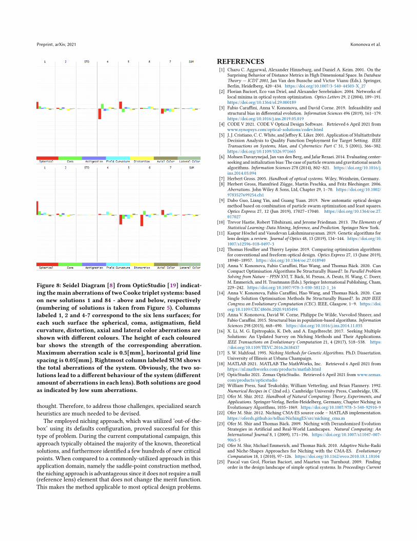
4.3 Optical Perspective of the Novel OptimaNew solutions identified by the proposed approach have been in-vestigated from the point of view of optics. At the first glance, allof them fall within the ‘morphological classes’ specified in [25](i.e., they have the same sequence of the signs of the lens surfacecurvatures). However, within such class, their exact performancediffers - Cooke triplets with curvatures specified by new solutionsdeliver numerically different aberrations [8] per lens, see Figure 8for an example. Further detailed analysis of the new solutions fromthe optics point of view is outside the scope of this paper.

Most of new solutions deliver not only low sum but also lowindividual (per lens) aberrations and, therefore, potentially can beused in industrial production and satisfy the aforementioned man-ufacturability constraints. Analysis of these individual aberrationshas made it clear that within the approach proposed in this pa-per additional constraints, additional objective or penalty termsin the existing objective function can be imposed to control suchindividual aberrations. This requires further study.

5 CONCLUSIONSIn this work we studied a basic instance of the Optical Lens Designproblem in light of the multiplicity of its solutions, and investi-gated the application of an existing niching approach to it. Ourstudy unveiled a fascinating real-world application as a testbed forrandomized search heuristics (and particularly black-box continu-ous solvers that operate on multimodal domains), and at the sametime, provided insights on the search landscape of this applicationdomain. Evidently, this low-dimensional optimization problem pos-sesses an underlying rough landscape, which is likely to get worseif larger lens design problems are to be considered. Altogether, thisproblem-instance is significantly more complex than previously

Preprint, arXiv, 2021 Kononova et al.

Figure 8: Seidel Diagram [8] from OpticStudio [19] indicat-ing themain aberrations of twoCooke triplet systems: basedon new solutions 1 and 84 - above and below, respectively(numbering of solutions is taken from Figure 5). Columnslabeled 1, 2 and 4-7 correspond to the six lens surfaces; foreach such surface the spherical, coma, astigmatism, fieldcurvature, distortion, axial and lateral color aberrations areshown with different colours. The height of each colouredbar shows the strength of the corresponding aberration.Maximum aberration scale is 0.5[mm], horizontal grid linespacing is 0.05[mm]. Rightmost column labeled SUM showsthe total aberrations of the system. Obviously, the two so-lutions lead to a different behaviour of the system (differentamount of aberrations in each lens). Both solutions are goodas indicated by low sum aberrations.

thought. Therefore, to address those challenges, specialized searchheuristics are much needed to be devised.

The employed niching approach, which was utilized ‘out-of-the-box’ using its defaults configuration, proved successful for thistype of problem. During the current computational campaign, thisapproach typically obtained the majority of the known, theoreticalsolutions, and furthermore identified a few hundreds of new criticalpoints. When compared to a commonly-utilized approach in thisapplication domain, namely the saddle-point construction method,the niching approach is advantageous since it does not require a null(reference lens) element that does not change the merit function.This makes the method applicable to most optical design problems.

REFERENCES[1] Charu C. Aggarwal, Alexander Hinneburg, and Daniel A. Keim. 2001. On the

Surprising Behavior of Distance Metrics in High Dimensional Space. In DatabaseTheory — ICDT 2001, Jan Van den Bussche and Victor Vianu (Eds.). Springer,Berlin, Heidelberg, 420–434. https://doi.org/10.1007/3-540-44503-X_27

[2] Florian Baciort, Eco van Driel, and Alexander Serebriakov. 2004. Networks oflocal minima in optical system optimization. Optics Letters 29, 2 (2004), 189–191.https://doi.org/10.1364/ol.29.000189

[3] Fabio Caraffini, Anna V. Kononova, and David Corne. 2019. Infeasibility andstructural bias in differential evolution. Information Sciences 496 (2019), 161–179.https://doi.org/10.1016/j.ins.2019.05.019

[4] CODE V 2021. CODE V Optical Design Software. Retrieved 6 April 2021 fromwww.synopsys.com/optical-solutions/codev.html

[5] J. J. Cristiano, C. C. White, and Jeffrey K. Liker. 2001. Application of MultiattributeDecision Analysis to Quality Function Deployment for Target Setting. IEEETransactions on Systems, Man, and Cybernetics: Part C 31, 3 (2001), 366–382.https://doi.org/10.1109/5326.971665

[6] Mohsen Davarynejad, Jan van den Berg, and Jafar Rezaei. 2014. Evaluating center-seeking and initialization bias: The case of particle swarm and gravitational searchalgorithms. Information Sciences 278 (2014), 802–821. https://doi.org/10.1016/j.ins.2014.03.094

[7] Herbert Gross. 2005. Handbook of optical systems. Wiley, Weinheim, Germany.[8] Herbert Gross, Hannfried Zügge, Martin Peschka, and Fritz Blechinger. 2006.

Aberrations. John Wiley & Sons, Ltd, Chapter 29, 1–70. https://doi.org/10.1002/9783527699254.ch1

[9] Dabo Guo, Liang Yin, and Guang Yuan. 2019. New automatic optical designmethod based on combination of particle swarm optimization and least squares.Optics Express 27, 12 (Jun 2019), 17027–17040. https://doi.org/10.1364/oe.27.017027

[10] Trevor Hastie, Robert Tibshirani, and Jerome Friedman. 2013. The Elements ofStatistical Learning: Data Mining, Inference, and Prediction. Springer New York.

[11] Kaspar Höschel and Vasudevan Lakshminarayanan. 2019. Genetic algorithms forlens design: a review. Journal of Optics 48, 13 (2019), 134–144. https://doi.org/10.1007/s12596-018-0497-3

[12] Thomas Houllier and Thierry Lepine. 2019. Comparing optimization algorithmsfor conventional and freeform optical design. Optics Express 27, 13 (June 2019),18940–18957. https://doi.org/10.1364/oe.27.018940

[13] Anna V. Kononova, Fabio Caraffini, Hao Wang, and Thomas Bäck. 2020. CanCompact Optimisation Algorithms Be Structurally Biased?. In Parallel ProblemSolving from Nature – PPSN XVI, T. Bäck, M. Preuss, A. Deutz, H. Wang, C. Doerr,M. Emmerich, and H. Trautmann (Eds.). Springer International Publishing, Cham,229–242. https://doi.org/10.1007/978-3-030-58112-1_16

[14] Anna V. Kononova, Fabio Caraffini, Hao Wang, and Thomas Bäck. 2020. CanSingle Solution Optimisation Methods Be Structurally Biased?. In 2020 IEEECongress on Evolutionary Computation (CEC). IEEE, Glasgow, 1–9. https://doi.org/10.1109/CEC48606.2020.9185494

[15] Anna V. Kononova, David W. Corne, Philippe De Wilde, Vsevolod Shneer, andFabio Caraffini. 2015. Structural bias in population-based algorithms. InformationSciences 298 (2015), 468–490. https://doi.org/10.1016/j.ins.2014.11.035

[16] X. Li, M. G. Epitropakis, K. Deb, and A. Engelbrecht. 2017. Seeking MultipleSolutions: An Updated Survey on Niching Methods and Their Applications.IEEE Transactions on Evolutionary Computation 21, 4 (2017), 518–538. https://doi.org/10.1109/TEVC.2016.2638437

[17] S. W. Mahfoud. 1995. Niching Methods for Genetic Algorithms. Ph.D. Dissertation.University of Illinois at Urbana Champaign.

[18] MATLAB 2021. MATLAB The MathWorks, Inc. Retrieved 6 April 2021 fromhttps://nl.mathworks.com/products/matlab.html

[19] OpticStudio 2021. Zemax OpticStudio. Retrieved 6 April 2021 from www.zemax.com/products/opticstudio

[20] William Press, Saul Teukolsky, William Vetterling, and Brian Flannery. 1992.Numerical Recipes in C (2nd ed.). Cambridge University Press, Cambridge, UK.

[21] Ofer M. Shir. 2012. Handbook of Natural Computing: Theory, Experiments, andApplications. Springer-Verlag, Berlin-Heidelberg, Germany, Chapter Niching inEvolutionary Algorithms, 1035–1069. https://doi.org/10.1007/978-3-540-92910-9

[22] Ofer M. Shir. 2012. Niching CMA-ES source code – MATLAB implementation.https://ofersh.github.io/telhai/NichingES/src/niching_cma.m

[23] Ofer M. Shir and Thomas Bäck. 2009. Niching with Derandomized EvolutionStrategies in Artificial and Real-World Landscapes. Natural Computing: AnInternational Journal 8, 1 (2009), 171–196. https://doi.org/10.1007/s11047-007-9065-5

[24] Ofer M. Shir, Michael Emmerich, and Thomas Bäck. 2010. Adaptive Niche-Radiiand Niche-Shapes Approaches for Niching with the CMA-ES. EvolutionaryComputation 18, 1 (2010), 97–126. https://doi.org/10.1162/evco.2010.18.1.18104

[25] Pascal van Grol, Florian Baciort, and Maarten van Turnhout. 2009. Findingorder in the design landscape of simple optical systems. In Proceedings Current

Addressing the Multiplicity of Solutions in Optical Lens Design as a Niching Evolutionary Algorithms Computational Challenge Preprint, arXiv, 2021

Developments in Lens Design and Optical Engineering X, Vol. 7428. SPIE OpticalEngineering + Applications, San Diego, California, United States, 742808–1–742808–11. https://doi.org/10.1117/12.825495

[26] Darko Vasiljevic. 2002. Classical and Evolutionary Algorithms in the Optimizationof Optical Systems. Springer, Boston, MA. https://doi.org/10.1007/978-1-4615-1051-2