Admission control of multi-class trafﬁc with service

Queueing Systems 27 (1997) 79–97 79

Admission control of multi-class traffic with servicepriorities in high-speed networks ∗

V.G. Kulkarni and N. Gautam

Department of Operations Research, University of North Carolina, Chapel Hill, NC 27599-3180, USAE-mail: {vg kulkarni;gautam}@unc.edu

Received 29 November 1995; revised 15 June 1997

We consider a fluid model of a system that handles multiple classes of traffic. The delayand cell-loss requirements of the different classes of traffic are generally widely differentand are achieved by assigning different buffers for different classes, and serving them in astrict priority order. We use results from the effective bandwidth of the output processes(see Chang and Thomas (1995)) to derive simple and asymptotically exact call-admissionpolicies for such a system to guarantee the cell-loss requirements for the different classesassuming that each source produces a single class traffic. We compare the admission-controlpolicies developed here with the approximate policy studied by Elwalid and Mitra (1995)for the case of two-class traffic.

Keywords: quality-of-service, fluid-flow models, effective bandwidth, multi-priority traffic,Chernoff dominant eigenvalue

1. Introduction

The concept of effective bandwidth and its use in the admission control for thestatistical multiplexing of bursty sources is now well-documented and accepted (seeGibbens and Hunt [11], Kesidis et al. [12], Elwalid and Mitra [8], Choudhury et al. [3],Whitt [18], etc.). In the emerging high-speed networks using asynchronous transfermode (ATM), each traffic-source is described by its stochastic characteristics, and isassured a quality of service (QoS), as measured by cell-loss probability, delay, delay-jitter, etc. The effective bandwidth is a number associated with a traffic-source suchthat if the sum of the effective bandwidths of all the sources multiplexed onto a bufferis less than the output rate of that buffer, then the QoS is satisfied for each source.

This method of admission control works quite satisfactorily as long as the QoSrequirements of the sources are the same or at least similar. Otherwise buffer-sizinghas to be done to assure the most stringent QoS for all the sources. This leads tounnecessarily large buffer sizes.

When the multiplexed traffic has widely differing QoS requirements (as will most

∗ This work was partially supported by NSF Grant No. NCR-9406823.

J.C. Baltzer AG, Science Publishers

80 V.G. Kulkarni, N. Gautam / Admission control of multi-class traffic

certainly be the case since the high-speed network is expected to carry all the traffic:video, voice and data) we need to look for other alternatives. There are two distinctcases that arise in applications.

In the first case (for example, the digitized voice with low-end bit-dropping, orMPEG2 video, or output from a leaky bucket) each source produces multi-class traffic,and although different classes can tolerate different cell-losses, the accepted traffic froma given source must reach the destination in the order in which it was generated. Thisnecessitates first-come-first-served scheduling at each node enroute. This kind of trafficrequirement is best handled by buffer-sharing schemes, or space-priority mechanisms(see Cidon et al. [4,5], Elwalid and Mitra [7], and Lin and Sylvester [16]). Kulkarniet al. [15] show that the effective bandwidth concept can be extended to effectivebandwidth vectors and used for admission control in this case.

In the second case each source produces a single-class traffic, but different sourceshave different QoS requirements. For example, real-time traffic has a more stringentdelay requirement but can tolerate higher cell-loss; while data traffic can tolerate higherdelay but demands much smaller cell losses. In such cases it is feasible to providea separate buffer for each class and service the real-time traffic buffer with higherpriority than the data-traffic buffer. Several service priorities are possible. The simplestscheduling discipline gives full priority to real-time traffic and the channel capacitythat is not used by the real-time traffic is made available to the data traffic.

In this paper we concentrate on this second case and consider a fluid model ofN distinct classes. There are Kj independent sources (j = 1, 2, . . . ,N ) producingfluid of type j that is multiplexed into a buffer of size Bj . The fluid is removed fromthese buffers following a static priority full service (SPFS) policy, i.e., fluid of type jis removed before fluid of type i if j < i. The main aim of this paper is to identifythe conditions under which the cell-loss probability requirement is satisfied for eachclass. We do this by using the results on the effective bandwidth of output processesas reported by de Veciana et al. [6], Chang and Thomas [1], and Chang and Zajic [2].

To do this we need to analyze multi-priority fluid models. Some work is alreadydone in this area: see Narayanan and Kulkarni [17] and Zhang [19]. A recent paper byElwalid and Mitra [9] provides an approximate way of solving the admission controlproblem for the two priority case. They approximate the busy periods of the high-priority buffers by exponential distributions to obtain tractable solutions, and showthat the approximation works quite well. They also incorporate the new results usingChernoff bounds in their analysis. Our results provide a simple admission controlcriterion that does not use the exponential approximation of Elwalid and Mitra [9].When there are two types of fluids, the SPFS policy is identical to the generalizedprocessor sharing scheduling discipline analyzed by Zhang et al. [20,21].

The rest of the paper is organized as follows. The next section restates some ofthe known results from large deviations. It also states an important characterization ofthe effective bandwidth of the output in terms of that of the input.

The multi-priority fluid model (with Kj sources of type j) is described in section 3to set the notation. We observe that the multi-priority model is identical to a tandem

V.G. Kulkarni, N. Gautam / Admission control of multi-class traffic 81

fluid model, where the fluid of type j and the output from the buffers 1, 2, . . . , j − 1are input to the jth buffer in tandem. This observation is also made in Elwalid andMitra [9] (for N = 2) and is immensely useful in our analysis.

The admission control criterion is formally derived in section 4. The main resultis given in theorem 3. An admission criterion that does not use the output analysisis even more simple and is shown to be conservative. Thus, the admission control inpractice can be done rather simply, using existing effective bandwidth formulae. Theresults are illustrated with an example of two classes of exponential on–off sources insection 5.

In section 6 the admission control is fine tuned using Chernoff bounds as statedin Elwalid et al. [9,10]. It takes into account the gain in statistical multiplexing.Three methods are stated to compute the relevant tail probabilities. The results aredemonstrated for a two-class exponential on–off source model in section 7. Numericalexamples are used to compare the three methods with each other and that in Elwalidand Mitra [9].

2. Preliminaries

Consider a single-buffer fluid model driven by a random environment {Z(t), t >0}. The buffer has infinite capacity and is serviced by a channel of constant capacity c.When the environment is in state Z(t), fluid enters the buffer at rate r(Z(t)). Let X(t)be the amount of fluid in the buffer at time t. The dynamics of the buffer contentprocess {X(t), t > 0} is described by

dX(t)dt

=

{r(Z(t))− c if X(t) > 0,{r(Z(t))− c}+ if X(t) = 0,

(1)

where {x}+ = max(x, 0).It has been shown in Kulkarni and Rolski [14] that the buffer content process

{X(t), t > 0} is stable if

E{r(Z(∞)

)}< c. (2)

Typically, in applications we are interested in satisfying a Quality of Servicecriterion that can be mathematically formulated as follows:

limt→∞

P(X(t) > B

)6 ε.

One can think of B as the finite buffer size and ε as the upper bound on the overflowprobability. It is known that (see Elwalid and Mitra [8], Gibbens and Hunt [11], andKesidis et al. [12]) in the asymptotic region, i.e., as B → ∞ and ε → 0, such that− log(ε)/B → δ > 0, there exists a quantity eb(δ), called the effective bandwidth ofthe input source, such that the QoS criterion is satisfied if

eb(δ) < c.


We recount below an important result by Kesidis et al. [12] that relates eb(δ) tothe input process. Let A(t) be the total fluid input until time t, where

A(t) =

∫ t

0r(Z(u)

)du.

Define

hA(v) = limt→∞

1t

logE{

exp(vA(t)

)}. (3)

Kesidis et al. [12] show that the effective bandwidth of the input is given by

ebA(δ) =hA(δ)δ

. (4)

They also state that hA(v) is an increasing, convex function of v.The important question is how to compute hA(·) for a given input process. El-

walid and Mitra [8], and Kesidis et al. [12] show how to do this when {Z(t), t > 0}is a Continuous Time Markov Chain (CTMC). Kulkarni [13] shows how to do thiswhen {Z(t), t > 0} is a Markov Regenerative Process (MRGP).

Now let D(t) be the total output from the buffer over [0, t]. In practice, D(t)may act as an input for a downstream buffer (e.g., in case of tandem queues). Henceit is useful to know the effective bandwidth of the output process. Analogous to (3),define

hD(v) = limt→∞

1t

logE{

exp(vD(t)

)}. (5)

Note that hD(v) is also a convex, increasing function and h′D(v) 6 c, since thepeak rate of the output process is bounded above by c, the channel-capacity.

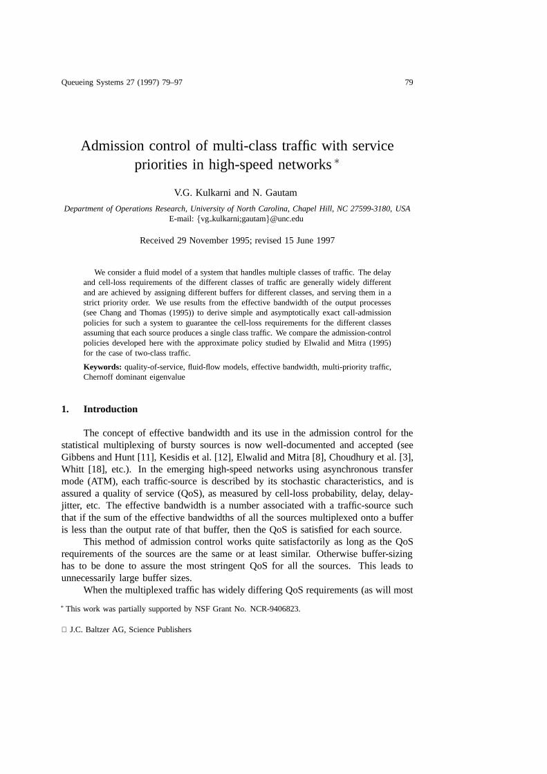
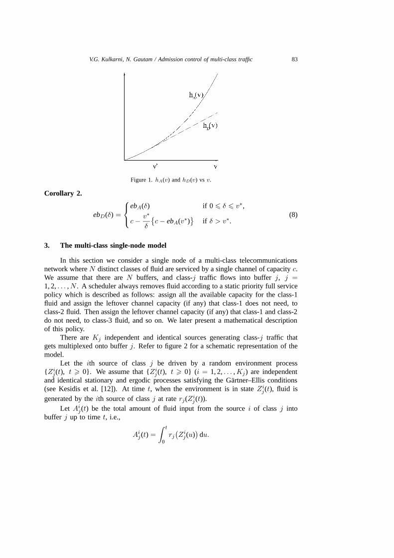
The next theorem (from Chang and Thomas [1], and, Chang and Zajic [2])establishes the relationship between hA(v) and hD(v). (h′A(v) denotes the derivativeof hA(v) with respect to v.)

Theorem 1. Suppose {Z(t), t > 0} is a stationary ergodic process satisfying theGartner–Ellis conditions (see Kesidis et al. [12]). Let v∗ satisfy

h′A(v∗) = c. (6)

Then

hD(v) =

{hA(v) if 0 6 v 6 v∗,hA(v∗)− cv∗ + cv if v > v∗.

(7)

See figure 1 for an illustration of hA(v) and hD(v). Using equation (4) we canrelate the effective bandwidth ebD(δ) of the output to the effective bandwidth ebA(δ)of the input.


Figure 1. hA(v) and hD(v) vs v.

Corollary 2.

ebD(δ) =

ebA(δ) if 0 6 δ 6 v∗,

c− v∗

δ

{c− ebA(v∗)

}if δ > v∗.

(8)

3. The multi-class single-node model

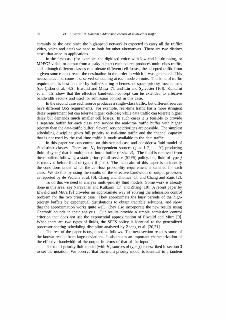
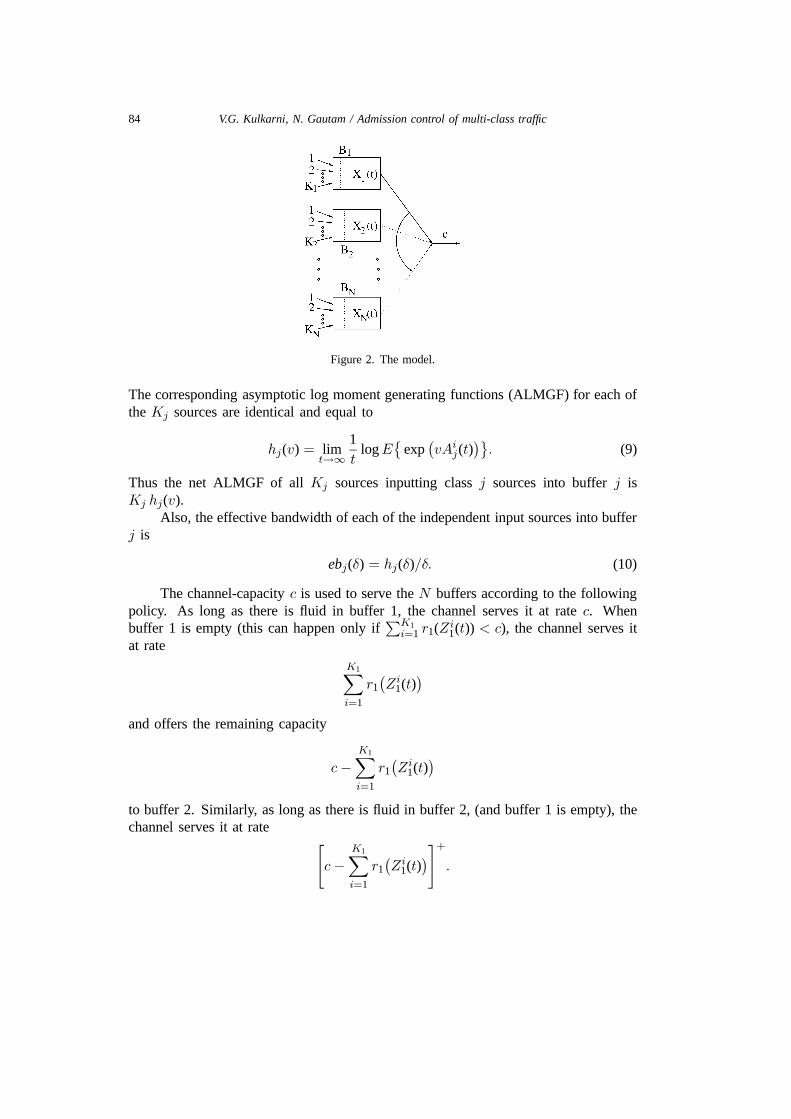
In this section we consider a single node of a multi-class telecommunicationsnetwork where N distinct classes of fluid are serviced by a single channel of capacity c.We assume that there are N buffers, and class-j traffic flows into buffer j, j =1, 2, . . . ,N . A scheduler always removes fluid according to a static priority full servicepolicy which is described as follows: assign all the available capacity for the class-1fluid and assign the leftover channel capacity (if any) that class-1 does not need, toclass-2 fluid. Then assign the leftover channel capacity (if any) that class-1 and class-2do not need, to class-3 fluid, and so on. We later present a mathematical descriptionof this policy.

There are Kj independent and identical sources generating class-j traffic thatgets multiplexed onto buffer j. Refer to figure 2 for a schematic representation of themodel.

Let the ith source of class j be driven by a random environment process{Zij(t), t > 0}. We assume that {Zij(t), t > 0} (i = 1, 2, . . . ,Kj) are independentand identical stationary and ergodic processes satisfying the Gartner–Ellis conditions(see Kesidis et al. [12]). At time t, when the environment is in state Zij(t), fluid isgenerated by the ith source of class j at rate rj(Zij(t)).

Let Aij(t) be the total amount of fluid input from the source i of class j intobuffer j up to time t, i.e.,

Aij(t) =

∫ t

0rj(Zij(u)

)du.


Figure 2. The model.

The corresponding asymptotic log moment generating functions (ALMGF) for each ofthe Kj sources are identical and equal to

hj(v) = limt→∞

1t

logE{

exp(vAij(t)

)}. (9)

Thus the net ALMGF of all Kj sources inputting class j sources into buffer j isKj hj(v).

Also, the effective bandwidth of each of the independent input sources into bufferj is

ebj(δ) = hj(δ)/δ. (10)

The channel-capacity c is used to serve the N buffers according to the followingpolicy. As long as there is fluid in buffer 1, the channel serves it at rate c. Whenbuffer 1 is empty (this can happen only if

∑K1i=1 r1(Zi1(t)) < c), the channel serves it

at rateK1∑i=1

r1(Zi1(t)

)and offers the remaining capacity

c−K1∑i=1

r1(Zi1(t)

)to buffer 2. Similarly, as long as there is fluid in buffer 2, (and buffer 1 is empty), thechannel serves it at rate [

c−K1∑i=1

r1(Zi1(t)

)]+

.


When buffer 2 is empty it is served at rate

min

{K2∑i=1

r2(Zi2(t)

),

[c−

K1∑i=1

r1(Zi1(t)

)]+}.

Similarly, as long as there is fluid in buffer 3, it gets served at rate[c−

K1∑i=1

r1(Zi1(t)

)−

K2∑i=1

r2(Zi2(t)

)]+

,

and so on.Let Xj(t) be the amount of fluid in the buffer j at time t. We shall analyze

the {Xj(t), t > 0} process assuming infinite buffers. Due to strict priority rules, wesee that {Xj(t), t > 0} does not depend upon Kj+1, . . . ,KN . We require a modifiedversion of the system stability condition as stated in Kulkarni and Rolski [14] as

limt→∞

N∑j=1

Kj∑i=1

E{rj(Zij(t)

)}< c. (11)

Let εj be the cell-loss-probability target for class-j traffic. Thus we want tosatisfy the following Quality-of-Service criteria for the N classes:

Gj(K1,K2, . . . ,Kj) = limt→∞

P(Xj(t) > Bj

)6 εj ,

where Bj is a given number (j = 1, 2, . . . ,N ).The main aim of the analysis in the next section is to identify the feasible region

K ={

(K1,K2, . . . ,KN ): G1(K1) 6 ε1, . . . ,GN (K1,K2, . . . ,KN ) 6 εN}. (12)

4. Analysis

We shall concentrate on the asymptotic region:

Bj →∞ and εj → 0, such that − log(εj)/Bj → δj > 0, j = 1, 2, . . . ,N.

We shall treat each of the priority cases separately.

• Priority 1. Since the priority-1 fluid gets uninterrupted service, the call-admissionpolicy is identical to the case where there is no other traffic. The effective band-width of K1 priority-1 fluid sources is given by K1 eb1(δ) (see (10)). It is knownthat the QoS criteria G1(K1) 6 ε1 is satisfied if

K1 eb1(δ1) < c. (13)


• Priority j (j = 2, 3, . . . ,N ). The capacity available to buffer j is 0 when at leastone of the buffers 1, 2, . . . , j − 1 is non-empty and it is[

c−j−1∑k=1

Kk∑i=1

rk(Zik(t)

)]+

if all the buffers 1, 2, . . . , j − 1 are empty. Let Rj−1(t) be the sum of the outputrates of the buffers 1, 2, . . . , j− 1 at time t. (Thus R0(t) = 0.) It can be seen that

Rj−1(t) =

{c if

∑j−1k=1Xk(t) > 0,

min[c,∑K1

i=1 r1(Zi1(t)

)]if∑j−1

k=1Xk(t) = 0.(14)

It is clear that the buffer j gets served with capacity c−Rj−1(t) at time t. Thus itis easy to see that the buffer j can be equivalently modeled as one that is servedat a constant rate c, but has an additional compensating source producing fluidat rate Rj−1(t) at time t. (The compensating source j is independent of the Kj

sources of priority j.) Since Rj−1(t) is the rate at which fluid is departing frombuffers 1, 2, . . . , j− 1, the effective bandwidth of the compensating source for thejth buffer, ebsj(δ), is equal to the effective bandwidth of the sum of the outputsof buffers 1, 2, . . . , j − 1. Note that ebs1(δ) = 0 for all δ. From corollary 2 ofsection 2, we have the effective bandwidth of the compensating source for bufferj recursively given by

ebs1(δ) = 0 for all δ,

ebsj(δ) =

Kj−1 ebj−1(δ) + ebsj−1(δ) if 0 6 δ 6 v∗j ,

c−v∗jδ

{c−Kj−1 ebj−1(v∗j )− ebsj−1(v∗j )

}if δ > v∗j ,

(15)

j > 2,

where v∗j is obtained by solving for v in the equation

ddv

[v(Kj−1 ebj−1(v) + ebsj−1(v)

)]= c.

Then the QoS criteria is satisfied for buffer j if

Kjebj(δj ) + ebsj(δj ) < c.

Combining the above results we get the following theorem.

Theorem 3. (K1,K2, . . . ,KN ) ∈ K (see equation (12)), i.e., the QoS criteria

Gj(K1,K2, . . . ,Kj) 6 εj , j = 1, 2, . . . ,N ,

are satisfied if

Kjebj(δj) + ebsj(δj ) < c, ∀j = 1, 2, . . . ,N , (16)


where ebs1(·) = 0, ebsj(·) is as in equation (15) and ebj(·) is as in equation (10).

Next we describe the approximation to K that eliminates the need to compute v∗jand ebsj(·). Let N be the set of points (K1,K2, . . . ,KN ) such that

N =

{(K1,K2, . . . ,KN ):

j∑k=1

Kkebk(δk) < c, for j = 1, 2, . . . ,N

}. (17)

Using (15) and the fact that hj(v) is an increasing, convex function, one can provethat ebsj(v) <

∑j−1i=1 Kiebi(v). Hence, we can easily prove the following theorem.

Theorem 4. N ⊂ K.

Thus the admission-control policy based on the simpler set of inequalities (17),rather than (16), is more conservative. We illustrate the results by means of an examplein the next section.

5. Exponential on–off sources

Consider the multiclass node (in section 3) with two classes of traffic. Class-1 isthe real-time traffic while class-2 is the non-real-time traffic. Class-1 traffic is givenhigher service priority over class-2 traffic. We assume that there are two buffers, withclass-j traffic coming into buffer j, j = 1, 2. A scheduler removes (capacity c) fluidfrom the buffers according to a static priority full service policy. Each of the Kj

class-j sources, j = 1, 2, are independent and identical on–off sources with exp(αj)on-times and exp(βj) off-times. When a class-j source is on, it generates fluid at raterj and when it is off, it generates fluid at rate 0.

From theorem 3 in section 4, we can derive the following results. (K1,K2) ∈ K(see equation (12)), i.e., the QoS criteria

G1(K1) 6 ε1, G2(K1,K2) 6 ε2

are satisfied if

(i) K1eb1(δ1) < c, and

(ii) K1eb1(δ2) +K2 eb2(δ2) < c if δ2 6 v∗,v∗

δ2K1eb1(v∗) +K2eb2(δ2) <

cv∗

δ2if δ2 > v∗,

(18)

where

v∗ =β1

r1

(√cα1

β1(K1r1 − c)− 1

)+α1

r1

(1−

√β1(K1r1 − c)

cα1

)


Figure 3. Feasible values of (K1,K2).

and (from Elwalid and Mitra [8] and Kesidis et al. [12])

ebj(δj) =rjδj − αj − βj +

√(rjδj − αj − βj)2 + 4βjrjδj

2δj.

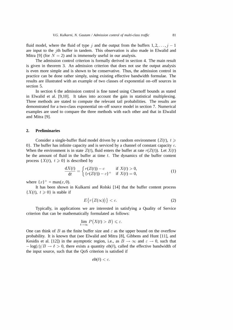
The acceptance region for the following numerical problem is shown in figure 3.

α1 = 2.4, β1 = 0.4, r1 = 2.0, ε1 = 10−7, B1 = 10,α2 = 1.0, β2 = 0.4, r2 = 1.2, ε2 = 10−5, B2 = 8 and c = 32.1.

Refer to figure 3 and inequalities (18). In region 1, K1r1 < c and hence v∗ =∞.Therefore (i) is trivially satisfied, and (ii) reduces to K1 eb1(δ2) +K2 eb2(δ2) < c. Inregion 2 K1r1 > c and δ2 6 v∗. Therefore we still use K1eb1(δ2) + K2eb2(δ2) < c.Now if δ2 > v∗ and we continue to use K1eb1(δ2) +K2eb2(δ2) < c we get region 3(bounded above by the dotted line). Instead, if we use

v∗

δ2K1eb1(v∗) +K2eb2(δ2) <

cv∗

δ2,

we get an extra set of feasible values of (K1,K2) that constitute region 4. Thus theregion K defined by (16) is the union of regions 1, 2, 3 and 4, while the approximateregion N , defined by (17) is the union of regions 1, 2 and 3. Note that N can besignificantly smaller than K.

6. Chernoff bounds

It can be shown that the region K (and hence of course N ) from the previoussections, is conservative, mainly because the statistical multiplexing gains are nottaken advantage of. In this section we show how we can use the Chernoff DominantEigenvalue (CDE) approximation (see Elwalid et al. [9,10]) to further fine tune the calladmission control problem analysis. The CDE approximation for the tail probability(for j = 1, 2, . . . ,N ) is given by

limt→∞

P(Xj(t) > Bj

)≈ Lje−ζjBj ,


where Lj is the fraction of the class j fluid that would be lost if there was no buffer.Mathematically Lj , j = 1, 2, . . . ,N , can be written as

Lj = limt→∞

∫ t0

{Rj−1(t) +

[∑Kji=1 rj

(Zij(t)

)]− c}+

dt∫ t0

{Rj−1(t) +

∑Kji=1 rj

(Zij(t)

)}dt

, (19)

where Rj−1(t) is the sum of the rates at which fluid is output from buffers 1, 2, . . . , j−1at time t as defined in (14) with R0(t) = 0 for all t. Note that Lj is a function of c,K1, . . . ,Kj , and the parameters of the sources of class j or less. Typically it may notbe computationally simple to calculate Lj exactly. Hence Elwalid et al. [10] suggesta method of estimating Lj by using Chernoff’s theorem. We explain it briefly below.

We characterize the input sources of class-j by a function mj(w), which is similarto hj(v) function, and is defined as

mj(w) = limt→∞

logE{

exp(wrj

(Zij(t)

))}. (20)

Note that mj(w) does not depend on i, for i = 1, 2, . . . ,Kj , since the Kj sources areidentical. Let

u∗j = supw>0

{cw −

N∑j=1

Kjmj(w)

}.

and w∗j be obtained by solving

N∑j=1

Kjm′j(w∗j ) = c.

Then the Chernoff estimate of Lj as given in Elwalid et al. [9,10] is

Lj ≈exp(−u∗j )

w∗jσ(w∗j )√

2π, (21)

where

σ2(w∗j ) =N∑j=1

Kjm′′j

(w∗j).

The main problem in the above analysis is computing mj(w). If {Zij(t), t > 0}can be modeled as a stationary and ergodic process with state space Sj and stationaryprobability vector, πj , we have

mj(w) = log

{∑k∈Sj

πkj ewrj(k)}. (22)

Then, we identify the new feasible region K using the following theorem.


Theorem 5. (K1,K2, . . . ,KN ) ∈ K, i.e., the QoS criteria

Gj(K1,K2, . . . ,Kj) = Lje−ζjBj 6 εj , j = 1, 2, . . . ,N ,

are satisfied if

Kjebj(ζj) + ebsj(ζj) < c, (23)

where ζj , j = 1, 2, . . . ,N , is given by

ζj = − log(εj/Lj)Bj

,

ebs1(·) = 0, ebsj(·) is as in equation (15) and ebj(·) is as in equation (10) with ebsj(v) =ebj(v) = 0 for v < 0.

We illustrate the above results with the following example.

7. CDE method for exponential on–off sources

In this section we consider the model of section 5 and show how the acceptanceregion changes with the choice of the method used to compute Lj . We also compare theresults obtained with those in Elwalid and Mitra [9]. Using the results from theorem 5in section 6, we get the following feasible region K.

(K1,K2) ∈ K, i.e., the QoS criteria

G1(K1) = L1e−ζ1B1 6 ε1, G2(K1,K2) = L2e−ζ2B2 6 ε2, (24)

are satisfied if

K1eb1(ζ1) < c, K2eb2(ζ2) + ebs2(ζ2) < c, (25)

where ζj , j = 1, 2, is given by

ζj = − log(εj/Lj)Bj

,

ebs2(v) =

K1 eb1(v) if 0 6 v 6 v∗,

c− v∗

v

{c−K1 eb1(v∗)

}if v > v∗,

0 if v < 0

(26)

and

ebj(v) =

rjv − αj − βj +√

(rjv − αj − βj)2 + 4βjrjv2v

if v > 0,

0 if v < 0.


Note that ζj would be negative when Lj < εj . We need to explicitly account for thispossibility.

The major effort in the above analysis lies in computing L1 and L2. We discussthree methods. The estimate of Li (i = 1, 2) obtained by method j (j = 1, 2, 3) isdenoted by L(j)

i . The feasible regions obtained by using L(j)1 and L(j)

2 is denoted by

K(j)={

(K1,K2): L(j)1 e−ζ1B1 6 ε1, L(j)

2 e−ζ2B2 6 ε2}.

Method 1. L(1)1 = 1 and L(1)

2 = 1. We know that L1 6 1 and L2 6 1, hence this is a

conservative estimate. Then the admissible region K(1)is the same as K in section 5

and is shown in figure 3.

Method 2. Using the independent on–off nature of the inputs of class-1, we can obtainan exact expression for L1 of equation (19) as

L(2)1 =

K1∑i=dc/r1e

(1− c

ir1

)K1!

i! (K1 − i)!(β1)i (α1)K1−i

(α1 + β1)K1. (27)

To compute L(2)2 , we use (21). First note that we analyze the buffer content process of

the second buffer by assuming that the output rate is always c and the input is fromK2 + 1 sources, viz., K2-exponential on–off sources of type 2 and one compensatingsource producing fluid at rate R1(t) at time t. Using equation (22) the m-function forthe K2 exponential on–off sources is seen to be

m2(w) = log

{α2

α2 + β2+

β2

α2 + β2ew r2

}. (28)

We show in appendix 1 that the m-function for the compensating source (see equa-tions (34) and (39)) is given by

m1(w) =

log{∑M

k=0 πk1 ewkr1

}if K1 6

⌊c

r1

⌋,

log{πM1 ewc +

∑M−1k=0 πk1 ewkr1

}if K1 >

⌊c

r1

⌋,

(29)

where M and the probabilities π01,π1

1, . . . ,πM1 are derived in appendix 1 (equations(32), (33) and (38)). Using m1(w) and m2(w), compute

u∗2 = supw>0

{cw −m1(w)−K2m2(w)

}and obtain w∗2 by solving

m′1(w∗2) +K2m′2(w∗2 ) = c.

Then compute L(2)2 using equation (21) and obtain the feasible region K(2)

.


Method 3. Compute L(3)1 = L(2)

1 . Instead of using Chernoff theorem to compute L2,we directly compute L(3)

2 by the following.If K1 6 bc/r1c,

L(3)2 =

K2∑k=d c−ir1

r2e

M∑i=0

πi1

(αK2−kβk

(α+ β)K2

)(ir1 + kr2 − cir1 + kr2

)K2!

k! (K2 − k)!

and if K1 > bc/r1c,

L(3)2 =

K2∑k=d c−ir1

r2e

(αK2−kβk

(α+ β)K2

)K2!

k! (K2 − k)!

M∑i=0

πi1

(1− c

min(c, ir1) + kr2

),

where M and the probabilities π01,π1

1, . . . ,πM1 are derived in the appendix (see equa-

tions (32), (33) and (38)). The admissible region obtained by this method is K (3).

Utilizing the fact that

L(3)1 = L(2)

1 6 L(1)1 = 1 and L(3)

2 6 L(2)2 6 L

(1)2 = 1,

we can easily prove the following theorem that summarizes the ordering of the regionsobtained in methods 1, 2 and 3.

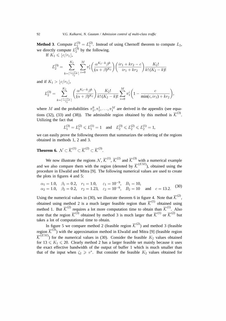
Theorem 6. N ⊂ K (1) ⊂ K (2) ⊂ K (3).

We now illustrate the regions N , K (1), K (2)

and K (3)with a numerical example

and we also compare them with the region (denoted by K (EM )), obtained using the

procedure in Elwalid and Mitra [9]. The following numerical values are used to createthe plots in figures 4 and 5:

α1 = 1.0, β1 = 0.2, r1 = 1.0, ε1 = 10−9, B1 = 10,α2 = 1.0, β2 = 0.2, r2 = 1.23, ε2 = 10−6, B2 = 10 and c = 13.2.

(30)

Using the numerical values in (30), we illustrate theorem 6 in figure 4. Note that K (2),

obtained using method 2 is a much larger feasible region than K (1)obtained using

method 1. But K (2)requires a lot more computation time to obtain than K (1)

. Alsonote that the region K (3)

obtained by method 3 is much larger that K (1)or K (2)

buttakes a lot of computational time to obtain.

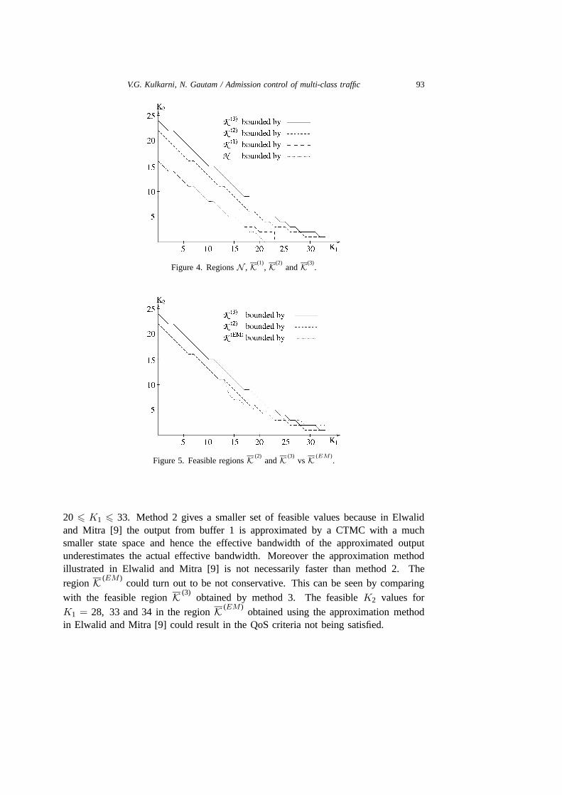
In figure 5 we compare method 2 (feasible region K (2)) and method 3 (feasible

region K (3)) with the approximation method in Elwalid and Mitra [9] (feasible region

K (EM )) for the numerical values in (30). Consider the feasible K2 values obtained

for 13 6 K1 6 20. Clearly method 2 has a larger feasible set mainly because it usesthe exact effective bandwidth of the output of buffer 1 which is much smaller thanthat of the input when ζ2 > v∗. But consider the feasible K2 values obtained for


Figure 4. Regions N , K(1), K(2)

and K(3).

Figure 5. Feasible regions K (2)and K (3)

vs K (EM).

20 6 K1 6 33. Method 2 gives a smaller set of feasible values because in Elwalidand Mitra [9] the output from buffer 1 is approximated by a CTMC with a muchsmaller state space and hence the effective bandwidth of the approximated outputunderestimates the actual effective bandwidth. Moreover the approximation methodillustrated in Elwalid and Mitra [9] is not necessarily faster than method 2. Theregion K (EM )

could turn out to be not conservative. This can be seen by comparingwith the feasible region K (3)

obtained by method 3. The feasible K2 values forK1 = 28, 33 and 34 in the region K (EM )

obtained using the approximation methodin Elwalid and Mitra [9] could result in the QoS criteria not being satisfied.


8. Conclusions

In this paper we have derived simple and asymptotically exact admission controlpolicies for the N -priority system with general sources. These policies use the standardeffective bandwidth formulae along with critical numbers v∗j , j = 2, 3, . . . ,N , forimplementation. A further simplification can be done that eliminates the use of v∗j ,and results in a more conservative policy. We have then used Chernoff bounds tofine tune the policies to obtain larger admissible regions. We have compared thedifferent approximations and simplifications to the admissible region. Depending onwhat kind of trade-off one would like to do between computational time and size ofthe feasible region, an appropriate method can be used. We have also illustrated howthe approximate policies reported by Elwalid and Mitra [9] compare with ours.

Note that it is possible to extend the computational results in section 7 to N > 2priorities. We consider the example of a 2-priority node firstly because it is easy toillustrate the results using a 2-dimensional graph, and secondly because comparableknown results are done for 2-priority cases only.

Appendix: Output process from buffer 1

To compute the m-function of the compensating source, we study the outputprocess from buffer 1. There are K1 independent and identical exponential on–offsources (with parameters α1, β1 and r1 as defined in section 5) that generate class 1fluid into buffer 1 and a channel serves the buffer at a maximum capacity c. Let N1(t)be the number of class 1 sources on at time t and X1(t) be the amount of class-1 fluidin the buffer 1 at time t. Define

Y (t) =

N1(t) if X1(t) = 0,⌈c

r1

⌉if X1(t) > 0.

(31)

Define

M = K1 if K1 6⌊c

r1

⌋and M =

⌈c

r1

⌉if K1 >

⌊c

r1

⌋. (32)

Let R1(t) be the output rate from buffer 1 at time t. We consider two cases:Case (i) K1r1 6 c. In this case M = K1, the buffer 1 is always empty, i.e.,

X1(t) = 0 for all t. The process {Y (t), t > 0} is a CTMC on {0, 1, . . . ,K1} andR1(t) = r1 Y (t) for all t. Therefore using (31), for i = 0, 1, 2, . . . ,K1,

πi1 = limt→∞

P{R1(t) = i r1

}= lim

t→∞P{N1(t) = i

}=

K1!i!(K1 − i)!

(β1)i(α1)K1−i

(α1 + β1)K1.

(33)


Then using equation (22),

m1(w) = log

{M∑k=0

πk1 ewkr1

}. (34)

Case (ii) K1r1 > c. In this case M = dc/r1e. We can see that the {Y (t), t > 0}process (see (31)) is a Semi-Markov Process (SMP) on state space {0, 1, . . . ,M} withkernel

G(t) =[Gi,j(t)

].

For i = 0, 1, . . . ,M − 1 and j = 0, 1, . . . ,M , let

Gi,j(t) =

iα1

iα1 + (K1 − i)β1

(1− exp

{−(iα1 +

(K1 − i)β1

)t})

if j = i− 1,

(K1 − i)β1

iα1 + (K1 − i)β1

(1− exp

{−(iα1 +

(K1 − i)β1

)t})

if j = i+ 1,

0 otherwise.

To describe GM ,j(t), we need to define the first passage time in {X1(t), t > 0} processas described below:

T = min{t > 0: X1(t) = 0

}.

Then for j = 0, 1, . . . ,M − 1, we have

GM ,j(t) = P{T 6 t, N1(T ) = j|X1(0) = 0, N1(0) = M

}.

(Note that GM ,M (t) = 0.)We need G(∞) = [Gi,j(∞)] in our analysis. We have for i = 0, 1, . . . ,M − 1

and j = 0, 1, . . . ,M ,

Gi,j(∞) =

iα1

iα1 + (K1 − i)β1if j = i− 1,

(K1 − i)β1

iα1 + (K1 − i)β1if j = i+ 1,

0 otherwise,

GM ,j(∞) = GM ,j(0),

(35)

where GM ,j(s) is the Laplace–Stieltjes transform (LST) of GM ,j(t), and can be com-puted using the analysis in Narayanan and Kulkarni [17].

We also need the expression for the sojourn time µi in state i, for i = 0, 1, . . . ,M .We have

µi =

1

iα1 + (K1 − i)β1if i = 0, 1, . . . ,M − 1,∑M−1

j=1 G′M ,j(0) if i = M .


Then we have for i = 0, 1, . . . ,M

πi1 = limt→∞

P{Y (t) = i

}=

piµi∑Mk=0 pkµk

, (36)

where

p = pG(∞).

It is easy to see that

R1(t) =

{r1 Y (t) if Y (t) < M ,c if Y (t) = M .

(37)

Therefore using (36) and (37), we have for i = 0, 1, . . . ,M

limt→∞ P{R1(t) = i} = limt→∞ P{Y (t) = i} =piµi∑Mk=0 pkµk

if i < M ,

limt→∞ P{R1(t) = c} = limt→∞ P{Y (t) = M} =pMµM∑Mk=0 pkµk

if i = M.(38)

Using the equations (22), (38) and (36), we see that

m1(w) = log

{πM1 ewc +

M−1∑k=0

πk1 ewkr1

}. (39)

References

[1] C.S. Chang and J.A. Thomas, Effective bandwidth in high-speed digital networks, IEEE Journal onSelected Areas in Communications 13(6) (1995) 1091–1100.

[2] C.S. Chang and T. Zajic, Effective bandwidths of departure processes from queues with time varyingcapacities, in: INFOCOM ’95 (1995) pp. 1001–1009.

[3] G.L. Choudhury, D.M. Lucantoni and W. Whitt, On the effectiveness of effective bandwidths foradmission control in ATM networks, in: Proceedings of ITC-14 (Elsevier Science, B.V., 1994)pp. 411–420.

[4] I. Cidon, R. Guerin and A. Khamisy, On protective buffer policies, Technical Report RC 18113,IBM Research Division (1992).

[5] I. Cidon, L. Georgiadis, R. Guerin and A. Khamisy, Optimal buffer sharing, IEEE Journal onSelected Areas in Communications 13(7) (1995) 1229–1240.

[6] G. de Veciana, C. Courcoubetis and J. Walrand, Decoupling bandwidths for networks: A decom-position approach to resource management, in: INFOCOM ’94 (1994) pp. 466–473.

[7] A.I. Elwalid and D. Mitra, Fluid models for the analysis and design of statistical multiplexing withloss priorities on multiple classes of bursty traffic, IEEE Trans. Communications 42(11) (1992)2989–3002.

[8] A.I. Elwalid and D. Mitra, Effective bandwidth of general Markovian traffic sources and admissioncontrol of high-speed networks, IEEE/ACM Trans. on Networking 1(3) (1993) 329–343.

[9] A.I. Elwalid and D. Mitra, Analysis, approximations and admission control of a multi-servicemultiplexing system with priorities, in: INFOCOM ’95 (1995) pp. 463–472.


[10] A.I. Elwalid, D. Heyman, T.V. Lakshman, D. Mitra and A. Weiss, Fundamental bounds and ap-proximations for ATM multiplexers with applications to video teleconferencing, IEEE Journal onSelected Areas in Communications 13(6) (1995) 1004–1016.

[11] R.J. Gibbens and P.J. Hunt, Effective bandwidths for the multi-type UAS channel, Queueing Systems9 (1991) 17–28.

[12] G. Kesidis, J. Walrand and C.S. Chang, Effective bandwidths for multiclass Markov fluids and otherATM sources, IEEE/ACM Trans. on Networking 1(4) (1993) 424–428.

[13] V.G. Kulkarni, Effective bandwidths for Markov regenerative sources, Queueing Systems 24 (1996)137–154.

[14] V.G. Kulkarni and T. Rolski, Fluid model driven by an Ornstein–Uhlenbeck Process, Probab. Engrg.Inform. Sci. 8 (1994) 403–417.

[15] V.G. Kulkarni, L. Gun and P.F. Chimento, Effective bandwidth vectors for multiclass traffic mul-tiplexed in a partitioned buffer, IEEE Journal on Selected Areas in Communications 13(6) (1995)1039–1047.

[16] A.Y.-M. Lin and J.A. Silvester, Priority queueing strategies and buffer allocation protocols fortraffic control at an ATM integrated broadband switching system, IEEE Journal on Selected Areasin Communications 9(9) (1991) 1524–1536.

[17] A. Narayanan and V.G. Kulkarni, First passage times in fluid models with an application to two-priority fluid systems, in: Proceedings of IPDS ’96 (1996).

[18] W. Whitt, Tail probabilities with statistical multiplexing and effective bandwidths for multiclassqueues, Telecommun. Syst. 2 (1993) 71–107.

[19] J. Zhang, Performance study of Markov-modulated fluid flow models with priority traffic, in:INFOCOM ’93 (1993) pp. 10–17.

[20] Z.L. Zhang, D. Towsley and J. Kurose, Statistical analysis of generalized processor sharing schedul-ing discipline, IEEE Journal on Selected Areas in Communications 13(6) (1995) 1071-80.

[21] Z.L. Zhang, D. Towsley and J. Kurose, Call admission control scheme under the generalized proces-sor sharing scheduling discipline, Technical Report UM-CS-95-10, University of Massachusetts(1995).

Documents

Admission control of multi-class trafﬁc with service