The Stewart PlatformThe Stewart-Gough or the Stewart Platform5 device is a six degree of freedom (mobility six) kinematic chain with closed loops. The kinematic chain consists of a base and a moving platform each of which is a spatial hexagon. See Figure 7. Every vertex of the base hexagon is connected to one vertex of the moving platform hexagon by one leg. Similarly, every vertex of the moving hexagon is connected to a vertex of the base hexagon by a leg. There are six such legs. Each leg has is a serial chain consisting of two revolute joints with intersecting axes, a prismatic joint and a spherical joint. Typically the prismatic joints are actuated.The mobility of a Stewart Platform can be easily verified to be six. Each leg has three linksand four joints. If we include the moving platform,n = 6 × 3+1 = 19.

The connectivity of the revolute and the prismatic joint is one. The connectivity of the sphericaljoint is three. There are 6 X 2 revolute joints, 6 prismatic joints and 6 spherical joints.The Stewart Platform has actuators for all its six prismatic joints and it is therefore possible tocontrol all six degrees of freedom.

Degrees of freedom of a systemThe number of independent variables (or coordinates) required to completely specify the configuration of the mechanical system. It is also the number of independent inputs required to drive all the rigid bodies in the mechanical system.

Kinematic chainA system of rigid bodies connected together by joints. A chain is called closed if it forms a closed loop. A chain that is not closed is called an open chain.

Serial chainIf each link of an open chain except the first and the last link is connected to two other links it is called a serial chain.

Connectivity of a jointThe number of degrees of freedom of a rigid body connected to a fixed rigid body through the joint. The revolute, prismatic and helical joints have a connectivity 1. The spherical joint has a connectivity of 3. Sometimes one uses the term “degree of freedom of a joint” instead of the connectivity of a joint.

Numerical ExampleCRS F3 is holding a plate. The plate is at location (0, 0, 200) in the tool coordinate system. At

the ready position, the tool coordinate system is at (500, 0, 600).

What is the location of the plate in the base coordinate system?

If the base is rotated 30° about Z0, what is the location of the plate?

0 = Tran (500, 0, 600) Rot(y, 90) N

= [ 0 0 1 5000 1 0 0

−1 0 0 6000 0 0 1

] [ 00

2001

] = [7000

6001

]0 = Rot (Z, 30) Tran (500, 0, 600) Rot(y, 90) N

= [0.866 −0.5 0 00.5 0.866 0 00 0 1 00 0 0 1

] [1 0 0 5000 1 0 00 0 1 6000 0 0 1

] [ 0 0 1 00 1 0 0

−1 0 0 00 0 0 1

] [ 00

2001

]= [433+173

250+100600

1] = [606

3506001

]If we swap the order of z rotation and translation, we will haveTran(433,250,600) Rot(z, 30) Rot(y,90).

The Denavit-Hartenberg Parameters in RoboticsThe Denavit-Hartenberg (D-H) framework is a method for assigning frames of reference

to a serial robot arm constructed of sequential rotary (and/or translational) joints connected with rigid links. If the robot arm is imagined at any fixed time, the axes about which the joints turn are viewed as lines in space. In the most general case, these lines will be skew, and in degenerate cases, they can be parallel or intersect.

In the D-H framework, a frame of reference is assigned to each link of the robot at the joint where it meets the previous link. The z-axis of the ith D-H frame points along the ith joint axis. Since a robot arm is usually attached to a base, there is no ambiguity in terms of which of

the two (±) directions along the joint axis should be chosen, i.e., the “up” direction for the first joint is chosen. Since the (i + 1)st joint axis in space will generally be skew relative to axis i , a unique x-axis is assigned to frame i, by defining it to be the unit vector pointing in the direction of the shortest line segment from axis i to axis i + 1. This segment intersects both axes orthogonally. In addition to completely defining the relative orientation of the ith frame relative to the (i − 1)st, it also provides the relative position of the origin of this frame.

The D-H parameters, which completely specify this model, are:

1. The distance from joint axis i to axis i + 1 as measured along their mutual normal.

This distance is denoted as ai .

2. The angle between the projections of joint axes i and i + 1 in the plane of their

common normal. The sense of this angle is measured counterclockwise around

their mutual normal originating at axis i and terminating at axis i + 1. This angle

is denoted as i .

3. The distance between where the common normal of joint axes i − 1 and i , and

that of joint axes i and i + 1 intersect joint axis i, as measured along joint axis i.

This is denoted as di.

4. The angle between the common normal of joint axes i − 1 and i , and the common

normal of joint axes i and i + 1. This is denoted as θi , and has positive sense

when rotation about axis i is counterclockwise.

Hence, given all the parameters {ai , αi , di , θi } for all the links in the robot, together with how

the base of the robot is situated in space, one can completely specify the geometry of the arm at

any fixed time. Generally, θi is the only parameter that depends on time.

In order to solve the forward kinematics problem, which is to find the position and

orientation of the distal end of the arm relative to the base, the homogeneous transformations of

the relative displacements from one D-H frame to another are multiplied sequentially. The

relative transformation, Hi−1 from frame i − 1 to frame i is performed by first rotating about the

x-axis of frame i −1 by αi-1, then translating along this same axis by ai−1. Next we rotate about the

z-axis of frame i by θi and translate along the same axis by di . Since all these transformations

are relative, they are multiplied sequentially on the right as rotations (and translations) about

(and along) natural basis vectors.

Motion Control

Motion control in NC machines is achieved by issuing coordinated motion commands to

the individual drives of the machine tool. Almost all commercial NC machines employ DC or

AC electrical motors that linearly drive stages/tables mounted on ball-bearing leadscrews. These

leadscrews provide low-friction (no stick-slip), no-backlash motions with accuracies of 0.001 to

0.005 mm or even better. High-precision machines employ interferometry- based displacement

sensors to provide sensory data to the (closed loop) controllers of the individual axes of the

machine tool (Chap. 13).

Rotational movements (spindle and other feed motions) are normally achieved using

high-precision circular bearings (plain, ball, or roller). Motion Types Machine tools can be

utilized to fabricate workpieces with prismatic and/or rotational geometries. Desired contours

are normally achieved through a controlled relative motion of the cutting tool with respect to the

work piece. Holes of desired diameters, on the other hand, are normally achieved by holding the

workpiece fixed and moving a rotating drill bit into the workpiece vertically. Correspondingly,

NC motions have been classified as point-to-point (PTP) motion (e.g., drilling) and contouring,

or continuous path (CP), motion (e.g., milling and turning).

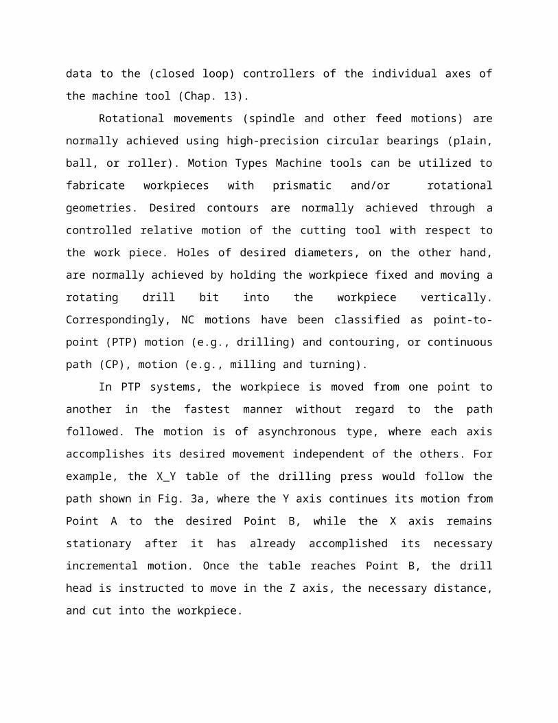
In PTP systems, the workpiece is moved from one point to another in the fastest manner

without regard to the path followed. The motion is of asynchronous type, where each axis

accomplishes its desired movement independent of the others. For example, the X_Y table of the

drilling press would follow the path shown in Fig. 3a, where the Y axis continues its motion

from Point A to the desired Point B, while the X axis remains stationary after it has already

accomplished its necessary incremental motion. Once the table reaches Point B, the drill head is

instructed to move in the Z axis, the necessary distance, and cut into the workpiece.

In CP systems, the workpiece (in milling) or the tool (in turning) follows a well-defined

path, while the material removal (cutting) process is in progress. All motion axes are controlled

individually and move synchronously to achieve the desired workpiece/tool motion (position and

speed). For example, the X_Y table of a milling machine would follow the path shown in Figure

3b, when continuously cutting into the workpiece along a two-dimensional path from Point A to

Point B.

For both PTP and CP motions, the coordinates of points or paths can be defined with

respect to a global (world) coordinate frame or with respect to the last location of the

workpiece/tool: absolute versus incremental positioning, respectively. Regardless of the

positioning system chosen, the primary problem in contouring is the resolution of the desired

path into multiple individual motions of the machine axes, whose combination would yield a

cutter motion that is closest possible to the desired path. This motion-planning phase is often

called interpolation. In earlier NC machine controllers, interpolation was carried out exclusively

in dedicated hardware boards, thus limiting the contouring capability of the machine tool to

mostly straight-line and circular-path motions. In modern CNC machines, interpolation is carried

out in software, thus allowing any desired curvature to be approximated by polynomial or spline-

fit equations.

FIGURE 3 (a) Point-to-point; (b) continuous path motion.

Trajectory Planning

As discussed above, a robotic manipulator is required to move either in PTP or in CP motion

modes in task space. However, robot motion control necessitates that commands be given in joint

space to yield a required task space end-effector path. We must plan individual joint trajectories

—joint displacement, velocity, and acceleration as a function of time, to meet this objective. PTP

and CP motions are treated separately below:

Point-to-Point Motion: In PTP motion, the robot end-effector is required to move from

its current point to another: a point is defined by a Cartesian frame location (position and

orientation—‘‘pose’’) with respect to a global (world) coordinate system (Fig. 14a). Although

the path followed is of no significance, except for avoiding collisions, all manipulator joints must

start and end their motions synchronously. Such a strategy would minimize acceleration periods

and thus minimize joint torque requirements— a phenomenon not considered in NC machining

due to the absence of significant inertial forces.

Trajectory planning for PTP motion starts by determining the joint displacement values at

both ends of the motion corresponding to the two end-effector Cartesian frames Fe1 and Fe2—

inverse kinematics, 1i and 2i, i=1, n, for an n-dof manipulator. The next step involves

determining individual joint trajectories: a vast majority of commercial robots only utilize

kinematics to determine these trajectories; only a very few utilize the dynamic models of the

manipulators. We will address both approaches below.

The dynamic model of the robot, clearly indicates that the availability of joint torques to

maximize joint velocities and accelerations is a function of the instantaneous robot configuration

and the geometry and mass of the object carried. In the absence of dynamic model utilization

during trajectory planning, one must therefore assume some logical limits for the joint velocities

and accelerations. Normally, worst-case values are utilized for these limits, i.e., assuming that

the robot configuration is in its most unfavorable configuration and carrying a payload of

maximum mass.

Based on these limits and user-defined joint trajectory velocity profiles, trapezoidal, or

parabolic, we must first determine the slowest joint, #k, i.e., the joint that will take the longest

time to accomplish its motion, k = 2k -1k. The time required to achieve k is defined as

the overall robot motion time for the end-effector to move from frame Fe1 to Fe2. All other

joints are slowed down to yield a synchronous motion for the robot that ends at time tf.

Continuous Point-to-Point Motion: In CPTP motion, the robot end effector is required to move

through all intermediate points (i.e., end-effector frames) without stopping and preferably

following continuous joint velocity profiles. A common solution approach to this problem is to

achieve velocity continuity at an intermediate point by accelerating/decelerating the joint motion

prior to getting to that point and in the process, potentially, not pass through the point itself but

only close to it. A preferred alternative strategy, however, would be the employment of spline

curves for the individual segments of the joint trajectory.

Through an iterative process, one can fit cubic or quintic splines to all the trajectories of

the robot’s n joints, while satisfying displacement, velocity, and acceleration continuity at all the

knots. The overall motion time can be minimized through an iterative process or using

parametric closed form equations, subject to all the joints’ individual kinematic constraints (i.e.,

max and ¨max).

Continuous Path Motion: In CP motion, the robot end-effector is required to follow a Cartesian

path, normally with a constant speed. The motion (translation and rotation) of the end-effector

frame is defined as a function of time. The solution of the (joint space) trajectory planning

problem for CP motion requires discretization of the Cartesian path in terms of a set of points

(frames) on this path separated by Cartesian distance and time. The robot can then be required to

carry out a CPTP motion through these points, as described above, whose corresponding joint

displacement values are determined by inverse kinematics.

In CPTP motion, however, the end-effector can be forced to pass only through the

selected set of points yielding a Cartesian path that approximates the desired path (e.g., a

straight-line motion with constant endeffector orientation with respect to the workpiece). If the

resultant path following errors in Cartesian space are greater than an acceptable threshold, we

would have to increase the number of points selected to approximate the desired path.

As a generalization of CP motion for real-time implementation, one can simply use the

inverse Jacobian matrix of the robot in determining joint velocities corresponding to the

instantaneous end-effector velocity requirements (Eq. 14.5). This method, originally proposed by

D. E. Whitney in the early 1970s, is commonly known as the resolved motion-rate-control

method. If at any instant, the robot’s dynamic capabilities cannot match the required end-effector

motion requirements, a tracking error results.

g-CodeA g-code program consists of a collection of statements/blocks to be executed in a sequential

manner. Each statement comprises a number of ‘‘words’’—a letter followed by an integer

number. The first word in a statement is the block number designated by the letter N followed by

the number of the block (e.g., N0027, for the 27th line in the g-code program). The next word is

typically the preparatory function designated by the letter G (hence, the letter ‘‘g’’ in g-code)

followed by a two-digit number. Several examples of G words are given in Table 1.

TABLE 1 Some G Words

Code Function Code Function

G00 Point-to-point motion

G01 Linear-interpolation motion

G02 Clockwise circular-interpolation

G03 Counterclockwise circular interpolation motion

G20 Imperial units

G21 Metric units

G32 Thread cutting motion

G98 Per-minute feed rate

G99 Per-revolution feed rate

The preparatory function is followed by dimensional words designated by axes’ letters X, Y, and

Z with corresponding dimensions, normally expressed as multiples of smallest possible

incremental displacements (e.g., X3712 Y-47000 Z12000; multiples of 0.01 mm) or in absolute

coordinates (e.g., X175.25 Y325.00 Z136.50). The feed rate and spindle speed words are

designated by the letters F and S, respectively, followed by the corresponding numerical values

in the chosen units. Next come the tool number word designated by the letter T and the

miscellaneous function word designated by the letter M (Table 2).

A typical g-code program block is

N0027 G90 G01 X175:25 Y325:00 Z136:50 F125 S800 T1712 M03 M08;

TABLE 2 Some M Words

M00 Program stop (during run)

M02 End of program

M03 Spindle start clockwise

M05 Spindle stop

M08 Coolant on

M11 Tool change

M98 Call a subprogram

M99 Return to main program

INTEGRATED AND AUTOMATED MANUFACTURING

Integrated manufacturing uses computers to connect physically separated processes. When

integrated, the processes can share information and initiate actions. This allows decisions to be

made faster and with fewer errors. Automation allows manufacturing processes to be run

automatically, without requiring intervention. This chapter will discuss how these systems fit

into manufacturing, and what role they play.

An integrated system requires that there be two or more computers connected to pass

information. A simple example is a robot controller and a programmable logic controller

working together in a single machine. A complex example is an entire manufacturing plant with

hundreds of workstations connected to a central database. The database is used to distribute work

instructions, job routing data and to store quality control test results. In all cases the major issue

is connecting devices for the purposes of transmitting data.

• Automated equipment and systems don’t require human effort or direction. Although this

does not require a computer based solution

• Automated systems benefit from some level of integration

Why Integrate?

There is a tendency to look at computer based solutions as inherently superior. This is an

assumption that an engineer cannot afford to entertain. Some of the factors that justify an

integrated system are listed below.

• a large organization where interdepartmental communication is a problem

• the need to monitor processes

• Things to Avoid when making a decision for integration and automation,

- ignore impact on upstream and downstream operations

- allow the system to become the driving force in strategy

- believe the vendor will solve the problem

- base decisions solely on financials

- ignore employee input to the process

- try to implement all at once (if possible)

• Justification of integration and automation,

- consider “BIG” picture

- determine key problems that must be solved

- highlight areas that will be impacted in enterprise

- determine kind of flexibility needed

- determine what kind of integration to use

- look at FMS impacts

- consider implementation cost based on above

• Factors to consider in integration decision,

- volume of product

- previous experience of company with FMS

- product mix

- scheduling / production mixes

- extent of information system usage in organization (eg. MRP)

- use of CAD/CAM at the front end.

- availability of process planning and process data

* Process planning is only part of CIM, and cannot stand alone.

ADVANTAGES OF AUTOMATION IN MANUFACTURING

In many cases there are valid reasons for assisting humans- tedious work -- consistency required- dangerous- tasks are beyond normal human abilities (e.g., weight, time, size, etc)- economics

• Advantages of Automated Manufacturing,- improved work flow- reduced handling- simplification of production- reduced lead time- increased moral in workers (after a wise implementation)- more responsive to quality, and other problems- etc.

• Various measures of flexibility,- Able to deal with slightly, or greatly mixed parts.

- Variations allowed in parts mix- Routing

flexibility to alternate machines- Volume flexibility- Design change flexibility

The Architecture of Integration

Integrated manufacturing systems are built with generic components such as,- Computing Hardware- Application Software- Database Software- Network Hardware- Automated Machinery

Manufacturing requires computers for two functions,- Information Processing - This is characterized by programs that can operate in a batchmode.- Control - These programs must analyze sensory information, and control devices while observing time constraints.

• An integrated system is made up of Interfaced and Networked Computers. The general structure is hierarchical: Corporate > Plant > Plant Floor >Process ControlThe plant computers tend to drive the orders in the factory.• The plant floor computers focus on departmental control. In particular,

- synchronization of processes.- downloading data, programs, etc., for process control.- analysis of results (e.g., inspection results).

• Process control computers are local to machines to control the specifics of the individual processes. Some of their attributes are,

- program storage and execution (e.g., NC Code),- sensor analysis,- actuator control,- process modeling,- observe time constraints (real time control).

To perform information processing and control functions, each computer requires connections,- Stand alone - No connections to other computers, often requires a user interface.- Interfaced - Uses a single connection between two computers. This is characterized by serial interfaces such as RS-232 and RS-422.- Networked - A single connection allows connections to more than one other computer. May also have shared files and databases.

• Types of common interfaces,- RS-232 (and other RS standards) are usually run at speeds of 2400 to 9600 baud, but theyare very dependable.

TABLE

1

Some G Wordsa

Code Function Code Function

G00 Point-to-point motion G20 Imperial units

G01 Linear-interpolation motion G21 Metric units

G02 Clockwise circular-

interpolation G32 Thread cutting

• Types of Common Networks,- IEEE-488 connects a small number of computers (up to 32) at speeds from .5 Mbits/sec to 8 Mbits/sec. The devices must all be with a few meters of one another.- Ethernet - connects a large number of computers (up to 1024) at speeds of up to 10 Mbits/sec., covering distances of km. These networks are LAN’s, but bridges may be used to connect them to other LAN’s to make a WAN.

• Types of Modern Computers,- Mainframes - Used for a high throughput of data (from disks and programs). These areideal for large business applications with multiple users, running many programs at once.- Workstations (replacing Mini Computers) - have multiprocessing abilities of Mainframe, but are not suited to a limited number of users.- Micro-processors, small computers with simple operating systems (like PC’s with msdos) well suited to control. Most computerized machines use a micro-processor

Manufacturing Automation Protocol was a computer network standard released in 1982 for interconnection of devices from multiple manufacturers. It was developed by General Motors to combat the proliferation of incompatible communications standards used by suppliers of automation products such as programmable controllers. By 1985 demonstrations of interoperability were carried out and 21 vendors offered MAP products. In 1986 the Boeing corporation merged its Technical Office Protocol with the MAP standard, and the combined standard was referred to as "MAP/TOP". The standard was revised several times between the first issue in 1982 and MAP 3.0 in 1987, with significant technical changes that made interoperation between different revisions of the standard difficult.Although promoted and used by manufacturers such as General Motors, Boeing, and others, it lost market share to the contemporary Ethernet standard and was not widely adopted. Difficulties included changing protocol specifications, the expense of MAP interface links, and the speed penalty of a token-passing network. The token bus network protocol used by MAP became standardized as IEEE standard 802.4 but this committee disbanded in 2004 due to lack of industry attention.