Embed Size (px)
Citation preview

Adnan Menderes UniversityFaculty of Arts And Sciences
Physics Department
PHYS 141 Physics LaboratoryLaboratory Manual
September, 2017AYDIN
1

.
Contents
1. Measurement of Basic Quantities: length, width, resistance and time...........6
2. Motion in One Dimension...............................................................................13
3. Projectile Motion............................................................................................19
4. Newton’s Second Law.....................................................................................24
5. Hooke’s Law....................................................................................................31
6. Ballistic Pendulum and Conservation of Energy..............................................37
7. Conservation of Momentum/Laws of Collision ..............................................41
8. Mechanical Conservation of Energy (Maxwell’s Wheel).................................47
2

Prepared by ;
• Experiments 1-7: Yelda Kadıoglu
• Experiments 2-3: Fatih Ersan
• Experiments 4-5: Onur Genc
• Experiments 6-8: S. Gokce Calıskan
Edited by ;
• Gonul Bilgec Akyuz
• Haydar Uncu
3

Notes For Students
The main aim of the general physics laboratory is to provide you with experimentalverification of various well known physical principles. They have been tested manytimes before, and there are accepted values for some of the physical quantities involvedin these principles. Your task in the laboratory is to compare your experimentallymeasured values to accepted theoretical or previously measured values.
Another purpose of the laboratory is to provide a vehicle to help you to search forand find relationships involved in a physical phenomena rather than just to try toreproduce precisely the accepted numerical value.
Also, one of the purposes of the laboratory is to give you an opportunity to be-come familiar with different measuring instruments and with methods for measuringphysical quantities like time, distance, velocity, acceleration, etc., to develop accu-rate results and at the same time to analyze the possible errors involved in makingmeasurements.
1 Laboratory Instructions
1. Remember at all times that the laboratory is a place for serious work. You willlearn a lot of useful things in the laboratory and develop skills necessary laterin your life.
2. The most important thing in the laboratory is your safety. Experiments aredesigned to be done safely, but necessary caution should always be exercised.The dangers mostly come from a lack of knowledge of the equipment and pro-cedures.
3. Upon entering the laboratory at the beginning of the laboratory period, youwill find the equipment on the tables. Restrain your curiosity and never playwith the equipment until it has been explained and permission has been givenby the instructor.
4. Most physics experiments are not dangerous, but a few are. Also, certain items,for example electricity, in various experiments can be especially dangerous.Equipment falling over is a common cause of accidents and therefore apparatusmust be properly placed and securely supported. Basic common sense andknowledge will keep you from all of the possible dangers.
5. Keep your apparatus and table top clean. Arrange your equipment properly,this will give you enough space to work easily, otherwise it will seem to beinsufficient.
6. The equipment provided for the laboratory experiment is expensive and some ofthe pieces are delicate. If they are used carelessly, certain pieces of apparatuscan be damaged easily. Personal safety rules also apply to equipment care.Even after you are familiar with the equipment, always have your experimentalset up checked and approved by instructor before putting it into operation.
7. If a piece of equipment is broken or does not function properly, report it to theinstructor.
4

8. Do not disassemble the set up until you are sure you have done everythingnecessary. After you complete the experiment, take the apparatus apart andleave the equipment neatly as you find it.
9. Good working habits are useful. Always read the whole description of an exper-iment before you come to the laboratory, so that you have a clear understandingof the experiment you are going to carry out.
10. Make sure you understand the purpose of the experiment. Keep the purposeclearly in mind and never forget it in the details of the procedure.
11. Repeat observations; whenever necessary, a few times while you carry out yourexperiment. Several readings are usually better than one.
12. In the experiments you will need the help of one or more partners. Discussthe results with your partners. You may learn more by working together on ananalysis than by doing it alone.
2 Grading Policy
Each experiment will be graduated upon 100 points.
(a) The student has an mini exam (approximately 15 minutes) for each ex-periment before performing the experiment. [30 points]
(b) The student will take experiment performance grades (This part also in-cludes oral exam). [30 points]
(c) The student prepare an experiment report. [40 points]
Average of these total grades will be your midterm exam.
Final exam include theoretical questions about each performed experiments,and will be at the end of semester.
3 Laboratory Reports
The laboratory report is a kind of manuscript to communicate your experimentresults and conclusions to other professionals. In this course you will write thelaboratory report to inform your LTA, so LTA can learn what you did andlearned from the experiment. But don’t write in your report like this sentence”In this experiment i learned the Ohm’s law · · · ”. Your laboratory reportshould be clear and concise. We prepare a report format as follow, you can useas a guide. In this lab probably you will work with more than one lab partners,but your report will be your individual effort.
3.1 Format of Laboratory Report
Name Surname:
Student Number:
5

Section and Experiment Date:
Laboratory Teaching Assistant Name: The name of the instructor whoyou have performed the experiment with.
Title of Experiment
Purpose In this part explain the purpose of the experiment briefly.
Theory In this part you can benefit from your lecture notes, books, etc. (Dontwrite more than one page for this part)
Apparatus In this part indicate which equipment was used while you performthe experiment.
Procedure In this part you will write how you perform this experiment in yourown words (not from laboratory manual)
Data and Calculations In this part you must write your data in order ( Youcan express them in a data-table format). You must write formulas that usedfor calculations, and your results must be written with significant numbers. Youmust write units of your all results in all steps of your calculations. You alsoplot graphs on graph paper (milimetric, logarithmic, etc.) in this part if neces-sary.
Conclusion In this part you must make a comment on your experiment andresults (and also on graphs). For example: you can evaluate and compare yourresults with theory, are they in agreement with physics laws, are your graphsas expected with respect to those laws? If there is error in your results, whatcan be the physical error causes? You must make comment also on those errorcauses.
Questions In this part you must answer questions about performed experimentwhich are in laboratory manual.
4 Symbols and Units of Some Fundamentals
In this course we will use SI (Systeme International) units for calculations.Some of the physical quantities are given in Table 1.
5 SIGNIFICANT FIGURES
The number of significant figures means the number of digits known in some number.The number of significant figures does not necessarily equal the total digits in thenumber because zeros are used as place keepers when digits are not known. Forexample, in the number 123 there are three significant figures. In the number 1230,
6

although there are four digits in the number, there are only three significant figuresbecause the zero is assumed to be merely keeping a place. Similarly, the numbers0.123 and 0.0123 both have only three significant figures. The rules for determiningthe number of significant figures in a number are:
• The most significant digit is the leftmost nonzero digit. In other words, zerosat the left are never significant.
• In numbers that contain no decimal point, the rightmost nonzero digit is theleast significant digit.
• In numbers that contain a decimal point, the rightmost digit is the least signif-icant digit, regardless of whether it is zero or nonzero.
• The number of significant digits is found by counting the places from the mostsignificant to the least significant digit.
As an example, the numbers in the following list of numbers all have four significantfigures. An explanation for each is given.
• 3456: All four nonzero digits are significant.
• 135700: The two rightmost zeros are not significant because there is no decimalpoint.
• 0.003043: Zeros at the left are never significant.
• 0.01000: The zero at the left is not significant, but the three zeros at the rightare significant because there is a decimal point.
• 1030.: There is a decimal point, so all four numbers are significant.
• 1.057: Again, there is a decimal point, so all four are significant.
• 0.0002307: Zeros at the left are never significant.
6 READING MEASUREMENT SCALES
Figure 1: A meter stick
For the measurement of any physical quantity such as mass, length, time, tempera-ture, voltage, or current, some appropriate measuring device must be chosen. Despite
7

the diverse nature of the devices used to measure the various quantities, they all havein common a measurement scale, and that scale has a smallest marked scale division.All measurements should be done in the following very specific manner. All metersand measuring devices should be read by interpolating between the smallest markedscale division. Generally the most sensible interpolation is to attempt to estimate 10divisions between the smallest marked scale division.
Consider the section of a meter stick pictured in Figure 1 that shows the regionbetween 2cm and 5cm. The smallest marked scale divisions are 1 mm apart. Thelocation of the arrow in the figure is to be determined. It is clearly between 3.4cmand 3.5cm, and the correct procedure is to estimate the final place. In this case areading of 3.45cm is estimated. For this measurement the first two digits are certain,but the last digit is estimated. This measurement is said to contain three significantfigures. Much of the data taken in this laboratory will have three significant figures,but occasionally data may contain four or even five significant figures.
8

Experiment 1Measurement of Basic Quantities: length,
width, resistance and time
1 Purpose
1. Demonstrate the specific knowledge gained by repeated measurements of thelength, weight, resistance and time.
2. Apply the statistical concepts of mean, standard deviation from the mean, andstandard error to these measurements.
Keywords: Mean value, standard deviation, standard error
2 Theory
No measuring device can be read to an unlimited number of digits. In addition whenwe repeat a measurement we often obtain a different value because of changes inconditions that we cannot control. The results of various measurements will spreadover a range of values. This spread is due to the errors in the measurements. Weare therefore uncertain as to the exact values of measurements. These uncertaintiesmake quantities calculated from such measurements uncertain as well.
The arithmetic mean, X, (or average) of a series of n measurements (Xi) is definedby :
X =1n
n∑
i=1
Xi (1)
Consider a case in which n measurements of the length and width are done. If Li
and Wi stand for the individual measurements of the length and width, and L andW stand for the mean of those measurements, so the equations relating them are:
L =1n
n∑
i
Li W =1n
n∑
i
Wi (2)
As mentioned above, in all measurements do have an error. Therefore we need alsoa way to determine the precision of the measurements. We get information aboutthe precision of the measurement from the variations of the individual measurementsusing the statistical concept standard deviation. The standard deviation is an indexof how closely the individual data points cluster around the mean. It is a measure ofthe dispersion, or scatter, of the data.
The standard deviation from the mean is defined as:
σX =
√√√√ 1n− 1
n∑
i=1
(Xi −X)2 (3)
9

The precision of the mean for X is given by the quantity called standard error, αX .In other words standard error is standard deviation of the mean value. This quantityis defined by the following equation:
αX =σX√
n(4)
Standard deviation reflects the variability of individual data points, and standarderror is the variability of means. Therefore, the result of the experiment is writtenas:
X = X ± αX (5)
which shows that the true value is most probably equal to X, but it can be in therange (X − αX , X + αX).
In experiments, one generally does more than one measurement and then usesthe results of these measurements to calculate to find the quantity that is to bemeasured. For example to find the momentum of an object one measures the massand the velocity of the object and multiply these quantities or to find the perimeterof a rectangle one measures the length and the width of the rectangle then sumthese two lengths and multiply by two, etc. Therefore we need how to proceed error(±αX) by doing these calculations. Propagation of error formula for multiplicationor division is given by:
Z = aX+bY ±c αZ
Z=
√b2(
αX
X)2 + c2(
αY
Z)2 (6)
For the case of an area that is the product of two measured quantities, the uncer-tainty in the area is related to the uncertainty of the length and width by:
Area = A = L×W αA =√
(L)2(αW )2 + (W )2(αL)2 (7)
Moreover, propagation of error formula for addition or subtraction is:
Z = X ± Y αZ =√
(αX)2 + (αY )2. (8)
THE VERNIER CALIPER
A vernier is a device that extends the sensitivity of a scale. It consists of a parallelscale whose divisions are less than that of the main scale by a small fraction, typically1/10 of a division. Each vernier division is then 9/10 of the divisions on the mainscale. The lower scale in Fig.1 is the vernier scale, the upper one, extending to 120mm is the main scale.
The left edge of the vernier is called the index, or pointer. The position of theindex is what is to be read. When the index is beyond a line on the main scale by1/10 then the first vernier line after the index will line up with the next main scaleline. If the index is beyond by 2/10 then the second vernier line will line up with thesecond main scale line, and so forth.
10

Figure 1: Vernier Caliper
If you line up the index with the zero position on the main scale you will see that theten divisions on the vernier span only nine divisions on the main scale. (It is alwaysa good idea to check that the vernier index lines up with zero when the caliper iscompletely closed. Otherwise this zero reading might have to be subtracted from allmeasurements.) Note how the vernier lines on either side of the matching line areinside those of the main scale. This pattern can help you locate the matching line.The sensitivity of the vernier caliper is then 1/10 that of the main scale. Keep inmind that the variability of the object being measured may be much larger than this.Also be aware that too much pressure on the caliper slide may distort the objectbeing measured.
THE MICROMETER CALIPER
Also called a screw micrometer, this measuring device consists of a screw of pitch0.5mm and two scales, as shown in Fig.2 . A linear scale along the barrel is dividedinto half millimeters, and the other is along the curved edge of the thimble, with 50divisions.
The pointer for the linear scale is the edge of the thimble, while that for the curvedscale is the solid line on the linear scale. The reading is the sum of the two parts inmm . The divisions on the linear scale are equal to the pitch, 0.5 mm. Since thiscorresponds to one revolution of the thimble, with its 50 divisions, then each divisionon the thimble corresponds to a linear shift of (0.50 mm)/50 = 0.01 mm.
In Fig.2 , the value on the linear scale can be read as 4.5 mm , and the thimblereading is 44×0.01 mm = 0.44 mm. The reading of the micrometer is then (4.50+0.44)mm = 4.94 mm.
Since a screw of this pitch can exert a considerable force on an object betweenthe spindle and anvil, we use a ratchet at the end of the spindle to limit the forceapplied and thereby, the distortion of the object being measured. The micrometerzero reading should be checked by using the ratchet to close the spindle directly onthe anvil. If it is not zero, then this value will have to be subtracted from all other
11
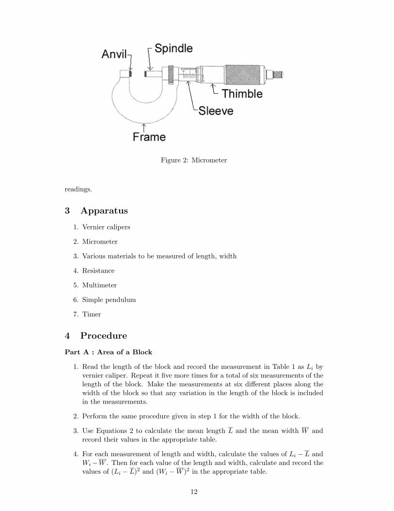
Figure 2: Micrometer
readings.
3 Apparatus
1. Vernier calipers
2. Micrometer
3. Various materials to be measured of length, width
4. Resistance
5. Multimeter
6. Simple pendulum
7. Timer
4 Procedure
Part A : Area of a Block
1. Read the length of the block and record the measurement in Table 1 as Li byvernier caliper. Repeat it five more times for a total of six measurements of thelength of the block. Make the measurements at six different places along thewidth of the block so that any variation in the length of the block is includedin the measurements.
2. Perform the same procedure given in step 1 for the width of the block.
3. Use Equations 2 to calculate the mean length L and the mean width W andrecord their values in the appropriate table.
4. For each measurement of length and width, calculate the values of Li − L andWi−W . Then for each value of the length and width, calculate and record thevalues of (Li − L)2 and (Wi −W )2 in the appropriate table.
12

5. Calculate σL, σW , αL, αW and record them in table.
6. Use the formula of Area = L ×W to calculate the value of area of the blockand record it in the appropriate table. Use Equation 7 to calculate the valueof αA.
Table 1:
Trial Li(m) Li − L(m) (Li − L)2 (m2) Wi(m) Wi −W (m) (Wi −W )2 (m2)123456
L =n∑
i=1(Li − L)2 = W =
n∑i=1
(Wi −W )2 =
σL = αL = L = L± αL =σW = αW = W = W ± αW =
A = L×W = αA = A = A± αA =
Part B : Volume of cylinderV olume = V = π × r2 × height
1. Measure the height and radius (1/2 diameter of a circle) of the cylinder bymicrometer or vernier, and record the measurement in Table 2 as Hi and ri
respectively.
2. Perform Steps in Part A for cylinder height and radius.
3. Calculate the volume of the cylinder.
Table 2:
Trial Hi (m) Hi −H (m) (Hi −H)2 (m2) ri(m) ri − r (m) (ri − r)2 (m2)123456
H =n∑
i=1(Hi −H)2 = r =
n∑i=1
(ri − r)2 =
σH = αH = H = H ± αH =σr = αr = r = r ± αr =
V = π × r2 ×H = αV = V = V ± αV
Part C : Period Measurement
13

1. Read the time for 10 complete oscillation of a simple pendulum by means of atimer and divide the time you measured by 10 to find the period of the simplependulum.
2. Perform step 1 five more times.
3. Calculate mean value, standard deviation and standard error of period of asimple pendulum.
Table 3:
Trial Ti(s) Ti − T (s) (Ti − T )2 (s2)12345
T =n∑
i=1(Ti − T )2 =
σT = αT = T = T ± αT =
Part D : Resistance Measurement
1. Read the value of resistance (R) by means of a multimeter.
2. Perform the procedure in part A for resistance.
3. Calculate mean value, standard deviation and standard error of a resistance.
Table 4:
Trial Ri(Ω) Ri −R(Ω) (Ri −R)2
12345
R =n∑1
(Ri −R)2 =
σR = αR = R = R± αR =
5 Questions
1. Learn the meaning of the keyword given in latin ”usus magister est optimus”.
2. Five students measure the mass of an object by making several measurements.These measurements are (in grams): 9.80, 9.87, 9.89, 9.95, 9.91, 9.98, 9.92,10.05, 9.97, 9.84. Calculate the mean, the standard deviation and standarderror.
3. If the standard deviation of a given data set is equal to zero, what can you sayabout the data values included in the given data set?
14

6 References
1. David H. Loyd, Physics Laboratory Manual
2. Juan Carlos Reina, Carol S. Monahan, Physics Experiments in Mechanic
15

Experiment 2Motion in One Dimension
1 Keywords
Vector, Distance, Displacement, Speed, Velocity, Acceleration.
2 Purpose
Investigation of position-time and velocity-time relation in one dimension.
3 Theory
This theoretical part is based on the corresponding chapter of “Physics Principles withApplications” (Douglas C. Giancoli).
Animals, balls, cars, and almost everything else in our environment are in motion,or can be in motion. The motion of objects was undoubtedly the first aspect of thephysical world to be thoroughly studied.
The study of motion is customarily divided into two parts: kinematics, whichdescribe the motion in terms of space and time while ignoring the agents that causethat motion, and dynamics, the reasons why a particular body moves as it does. Thisexperiment deals with kinematics. To describe the motion of an object we will needin addition to distance and time, two concepts: velocity (or speed) and acceleration.In this experiment we will discuss objects that move without rotating. Such motionis called translational motion. We will also restrict ourselves mainly to linear motion- that is, to motion along a straight line for this experiment.
3.1 Reference frames and coordinate systems
When riding in a train you may observe a bird flying by overhead and remark thatit looks as if it is moving at a speed of 30km/h. But do you mean it is traveling30km/h with respect to the train, or with respect to the ground?
Every measurement must be made with respect to a frame of reference. Forexample, while on a train traveling at 80km/h, you may notice a person passing youby walking toward the front of the train at a speed, of say, 5 km/h. Of course this isthe person’s speed with respect to the train. With respect to the ground, that personis moving at 85km/h. It is always important to specify the frame of reference whenstating a speed. We almost always mean ”with respect to the earth” without eventhinking about it, but the reference frame should be specified whenever there mightbe confusion.
The values of other physical quantities also depend on the frame of reference. Forexample, there is no point in telling you that Izmir is 110km away unless specifying110km from where. Distances are always measured in some frame of reference. Fur-thermore, when specifying the motion of an object, it is important to specify not onlythe speed but also the direction of motion. Therefore, in physics we often draw a setof coordinate axes as shown in Figure 1, to represent a frame of reference. Objects
16

O+ x- x
+ y
- y
Figure 1: Standard (Cartesian) set of coordinate axes.
positioned to the right of the origin of coordinates (O) on the x axis are usually saidto have an x coordinate with a positive value and positioned to the left of origin anegative value. The position along the y axis is usually considered positive whenabove and negative when below O, although the reverse convention can be used ifconvenient. Any point on the plane can then be specified by giving its x and y co-ordinates. In three dimensions, a z axis perpendicular to the x and y axes is alsoused.
3.2 Vectors
A quantity which has direction as well as a magnitude, is called a vector. However,many quantities such as time, have no direction associated with them; they only havea magnitude; that is, they are specified completely by giving a number (and units, ifany). Such quantities are called scalars.
3.3 Distance vs. Displacement
As an object moves, its location undergoes a change. There are two quantities thatare used to describe the changing location. One quantity - distance - accumulatesthe amount of total change of location over the course of a motion. Distance isthe amount of ground that is covered. The second quantity - displacement - onlyconcerns itself with the initial and final position of the object. Displacement is theoverall change in position of the object from start to finish and does not concern itselfwith the accumulation of distance traveled during the path from start to finish.
3.4 Speed vs. Velocity
Speed and velocity are two quantities in physics that seem at first glance to have thesame meaning. Although related, they have distinctly different definitions. Knowingtheir definitions is critical to understanding the difference between them.
Speed is a quantity that refers to how far an object moves in a given time interval,and that describes how fast or how slow an object is moving. In general, the averagespeed of an object is defined as the distance traveled divided by the time it takes totravel this distance:
Average speed =distance traveled
time elapsed(1)
17

This definition can be written briefly as:
v =d
t, (2)
where d stands for distance, t for the elapsed time and v for speed (v is the abbre-viation for the word velocity). The bar over the v is the standard symbol meaning”average.”
Another term is instantaneous speed. Instantaneous speed can be defined moreprecisely as the average speed over a very short time interval -an interval so shortthat the speed can be considered not to change during that short time. We can statethis in shorthand (or algebraic) terms by making use of the Greek letter ∆ (delta) tomean ”small change in” or ”small amount of.” Then:
v =∆d
∆t[∆t very small, approaching zero (∆t → 0)], (3)
Here v represents the instantaneous speed, and ∆d represents the small distancetraveled during the very short time interval ∆t.
Velocity is used to signify both the magnitude (numerical value) of how fast anobject is moving and its direction. Speed, on the other hand, has a magnitude only.There is a second difference between speed and velocity: namely, the magnitudeof the average velocity is defined in terms of ”displacement (~d),” rather than totaldistance traveled (d); that is
Average velocity =displacement
time elapsed(4)
where displacement means the net distance of the object from the starting point aftera given elapsed time. To see the distinction between the distance (which is used incalculating the speed) and the displacement (used for the velocity), imagine a personwalking 50 meters (m) to the east and then turning around and walking back (west) adistance of 10 m. The total distance traveled is 60 m but the displacement is only 40m since the person is now only 40 m for from the starting point. If this walk took 40seconds (s), the average speed was (60 m)/(40 s)=1.5 m/s, but the average velocityin this case was (40 m)/(40 s)=1.0 m/s. This discrepancy between the magnitudeof velocity and the speed occurs in some cases, but only for the average values andwe rarely need to be concerned with it. The magnitude of the instantaneous velocityand the instantaneous speed are always the same. The instantaneous velocity isdefined, like instantaneous speed. It equals the limiting of the ratio ∆~d/∆t as ∆tapproaches zero and in calculus notation, this limit is called the derivative of ~d withrespect to t, written as:
~v = lim∆t→0
∆~d
∆t=
~ds − ~di
ts − ti=
d~d
dt, (5)
3.5 Acceleration
The definition of acceleration involves the change in velocity. Thus an accelerationresults not only when the magnitude of the velocity changes but also if the directionchanges. For example, a person riding in a car traveling at constant speed arounda curve or a child riding o a merry-go-round, will both experience an accelerationbecause of a change in the direction of the velocity.
18

The average acceleration ~a of the particle is defined as the change in velocity ∆~vdivided by the time interval ∆t during which that change occurs:
~a =∆~v
∆t(6)
Using this definition, one can immediately define instantaneous acceleration as:
~a = lim∆t→0
∆~v
∆t=
d~v
dt(7)
One Dimensional Motion with Constant Acceleration:If the acceleration of a particle varies in time, its motion is complex and difficult to
analyze. However, a very common and simple type of one dimensional motion is theone in which the acceleration is constant. When this is the case, the average acceler-ation over any time interval is numerically equal to the instantaneous acceleration atany instant within the interval, and the velocity changes at the same rate throughoutthe motion.
4 Apparatus
1. Timer 4-4
2. Light barrier
3. Air track rail
4. Glider for air track
5. Magnet with plug for starter system
5 Procedure
1. Set up the apparatus like shown in figure 2.
2. Fix the positions of sensors such that the distance between successive ones willbe equal to each other (for example 15cm) and perform all your measurementswith these positions.
3. While d1 = d2 = d3 = d4 is the magnitude of the length of the black card (weassume this length as displacement) which is hang off to glider and t1, t2, t3,t4 are the time at which car passes the corresponding glider. Measure thesevalues for 3 different levels of the button (which includes magnet with plug forstarter system) and write them in Table 1. Don’t forget to write their units.
4. Calculate the average velocity and average acceleration and write them in Table2. Don’t forget to write their units.
5. Draw d-t and v-t graphs on a millimetric paper and make comments for graphs.
Table 1: Magnitude of displacement and time
d1 ( ) d2 ( ) d3 ( ) d4 ( ) t1 ( ) t2 ( ) t3 ( ) t4 ( )1th level2th level3rd level
19

Figure 2: Experiment set-up.
Table 2: Magnitude of velocity and acceleration
v1 ( ) v2 ( ) v3 ( ) v4 ( ) a1 ( ) a2 ( ) a3 ( ) a4 ( )1th level2th level3rd level
6 Questions
1. Categorize the following quantities by placing them under one of the two columnheadings.
displacement, speed, force, momentum, energy, acceleration, distance, velocity,temperature, time.
Scalars Vectors
2. True or False: An object may be moving for 10 seconds and still have zerodisplacement.
If the above statement is true, then describe an example of such a motion. Ifthe above statement is false, then explain why it is false with giving an exampleof such a motion.
3. True or False: It is possible for an object to move for 10 seconds at a highspeed and end up with an average velocity of zero.
20

If the above statement is true, then describe an example of such a motion. Ifthe above statement is false, then explain why it is false with giving an exampleof such a motion.
7 References
1. Physics Principles with applications, Douglas C. Giancoli, Prentice-Hall, Inc.Englewood Cliffs, New Jersey 07632.
2. Phywe, Physics Laboratory Experiments Manual.
21

Experiment 3Projectile Motion
1 Keywords
Gravitational Force, Two Dimensional Motion, Range.
2 Purpose
A steel (and wooden) ball is fired by a spring at different velocities and at differentangles to the horizontal. The relationships between the range, the height of projec-tion, the angle of inclination, and the firing velocity are determined. Our purposeis
1. To determine the range as a function of the angle of inclination.2. To determine the maximum height of projection as a function of the angle of
inclination.3. To determine the (maximum) range as a function of the initial velocity.
3 Theory
This theoretical part is based on the corresponding chapters of “Physics Principleswith Applications” (Douglas C. Giancoli) and “PHYSICS for Scientists and Engi-neers with Modern Physics” (Raymond A. Serway, John W. Jewett, Jr.)
In the previous experiment, we have discussed only motion in a straight line, andthe net force exerted on objects (if you don’t ignore the friction) was along the lineof motion. If the force on an object acts sideways to the direction of motion, thenthe object will move in a curved path. This is the situation occurs when an object isprojected into the air at an angle other than vertical in this case, the object is actedon by the force of gravity. A thrown football, a speeding bullet, and propagation ofa charged particle in a uniform electric field are all examples of projectiles.
It was Galileo who realized that projectile motion could be understood by analyzingthe horizontal and vertical components of the motion separately. If a body of massmoves in a constant gravitational field (gravitational force, ~Fgravity = m~g), the motionlies in a plane as in Figure 1. In this experiment we will ignore air resistance. Thevelocity vector at each instant points in the direction of the motion at that instantand hence is always tangent to the path.
For a given initial velocity, ~v0 and initial position, ~s0, the position of a particle, ~s,as a function of time, undergoing constant acceleration, ~a is given by
~s = ~s0 + ~v0t +12~at2 (1)
This is a vector equation and can be broken up into its x, y, and z components. Sincethe motion is in a plane, we need only look at the x and y components. If we neglectair resistance, the acceleration in the y direction is -g, due to gravity. The accelerationin the x direction is zero. Therefore, we can express acceleration as ~g = 0~i + (−g)~j.When analyzing projectile motion, we model it to be the superposition of two motions:
22

y
x
v =0yOA
V0
h
θ
R
OA
OBO
Figure 1: Trajectory of projectile motion.
(i) motion of a particle under constant velocity in the horizontal directionand (ii) motion of a particle under constant acceleration (free fall) in thevertical direction. The horizontal and vertical components of a projectiles motionare completely independent of each other and can be handled separately, with time tas the common variable for both components. Hence, the vector equation (1) becomestwo scalar equations:
x = x0 + v0xt (2)
y = y0 + v0yt− 12gt2 (3)
In terms of the angle θ, and the initial speed v0 the initial velocity components are
v0x = v0cosθ = constant , v0y = v0sinθ − gt (4)
Let us assume that a projectile is launched from the origin at ti = 0 with a positivev0y component as shown in Figure 1 and returns to the same horizontal level. Twopoints are especially interesting to analyze: the peak point (A), which has Cartesiancoordinates (R/2, h), and the point (B), which has coordinates (R, 0). The distanceR is called the horizontal range of the projectile, and the distance h is its maximumheight. Let us find h and R mathematically in terms of v0 , θ , and g.
We can determine h by noting that at the peak vy(A) = 0. Therefore, we can usethe equality for the y component of Equation 4 to determine the time t(A) at whichthe projectile reaches the peak:
0 = v0sinθ − gt(A) so t(A) =v0sinθ
g(5)
Substituting this expression for t(A) into the Equation 3 and replacing y − y(A)
with h, we obtain an expression for h in terms of the magnitude and direction of theinitial velocity vector:
23

h = (v0sinθ)v0sinθ
g− 1
2g(
v0sinθ
g)2 , h =
(v0)2sin2θ
2g(6)
The time spent by the projectile until it reaches to the range R is twice the timeat which it reaches its peak, that is, t(B) = 2t(A). Using the Equation 2 and notingthat v0x = v(xB) = v0cosθ, and setting x(B) = R at t = 2t(A), we find that
R = v0xt(B) = v0cosθ2t(B) = (v0cosθ)2v0sinθ
g=
2(v0)2sinθcosθ
g(7)
Using the identity sin 2θ = 2sinθcosθ, we can write R in the more compact form
R =(v0)2sin2θ
g(8)
The maximum value of R obtained by Equation 8 is Rmax = (v0)2/g. Since themaximum value of sine function is 1 and it is reached when 2θ = 90 , the maximumof the range R occurs when θ = 45 .
4 Apparatus
1. Ballistic unit
2. Recording paper
3. Steel ball, hardened and polished, d = 19 mm
4. Two tier platform support
5. Meter Scale
6. Barrel base
7. Speed measuring attachment
8. Power supply 5 VDC/2.4 A with DC-socket 2.1 mm
5 Procedure
1. Set up the apparatus like shown in Figure 2.
2. Try to level heights of the platform and ball position.
3. Place the steel ball to the leaper and adjust it at 75 . Perform your experimentfor three levels of leaper, measure the range with a ruler, read initial velocityfrom screen and write them into the Table 1. Calculate the theoretical rangefrom the equation 8. Find the percentage errors and write all your results toTable 1. Don’t forget to write their units.
4. Repeat the experiment again with the steel ball at first level for various anglevalues (15 , 30 , 45 , 60 , 75 ). Using the obtained initial velocity calculatethe theoretical maximum height and range from equations 6 and 8, respectively.Find the percentage errors of your experiments for the ranges. Write your allresults in Table 2. Don’t forget to write their units.
24

Figure 2: Set-up of Projectile motion experiment.
5. Repeat procedure 4 with wooden ball. Write your all results in Table 3. Don’tforget to write their units.
6. Plot R vs v0 for steel ball for procedure 3 in millimetric paper and makeyour comments for graphs.
7. Plot R vs θ for both steel and wooden balls in millimetric paper and makeyour comments for graphs.
Table 1: For steel ball and 75
First level Second level Third levelv0( )R( )
Rtheoretical( )PercentageError( )
Table 2: For steel ball and various angles (15 , 30 , 45 , 60 , 75 )
15 30 45 60 75
v0( )R( )
Rtheoretical( )PercentageError( )
hmax(theoretical)
25

V
Figure 3: Draw in the x- and y-components of velocity and acceleration.
Table 3: For wooden ball and various angles (15 , 30 , 45 , 60 , 75 )
15 30 45 60 75
v0( )R( )
Rtheoretical( )PercentageError( )hmax(theoretical)( )
6 Questions
1. Draw the x- and y- components of the velocity and acceleration for each dotalong the path of the cannonball in Figure 3. The velocity component for thefirst dot is done for you.
2. State which of the following quantities, if any, remain constant as a projectilemoves through its parabolic trajectory: (a) speed (b) acceleration (c) horizontalcomponent of velocity (d) vertical component of velocity.
3. An artillery shell is fired with an initial velocity of 100 m/s at an angle of 30
above the horizontal. Find (a) its position and velocity after 8s (b) the timerequired to reach its maximum height (c) the horizontal distance (R).
4. Discuss how the air resistance changes the motion of a projectile.
7 References
1. Physics Principles with applications, Douglas C. Giancoli, Prentice-Hall, Inc.Englewood Cliffs, New Jersey 07632.
2. Physics for Scientists and Engineers with Modern Physics, Raymond A. Serway,John W. Jewett, Jr.
3. Phywe, Physics Laboratory Experiments Manual.
26

Experiment 4Newton’s Second Law
1 Purpose
To examine the Newton’s second law in the manner of the physical relations; position-time, velocity-time, total mass-acceleration, and force-acceleration.
1.1 Keywords
Vector, magnitude (strength) of a vector, force, external force, internal force, gravi-tational force, weight, mass, acceleration, velocity, speed, position vector, Newton’sLaws (first, second & third)
2 Theory
The fundamental principle of the dynamics (The Second Law of Newton) for a con-stant mass m(t′) ≡ m ≡ [constant] with an external net force ~F (t′) acting on it, isexspressed in terms of the acceleration ~a(t′) by;
~F (t′) = m~a(t′) (1)
on the other hand;
~a(t′) =d2~r(t′)dt′2
(2)
where ~r(t′) is the position vector of the mass m. Hence the Newtons’s Second Lawcan be expressed in the differential equation form as;
~F (t′) = md2~r(t′)dt′2
(3)
Then from the above equation;
~F (t′) = md2~r(t′)dt′2
= md
dt′
(d~r(t′)dt′
)
⇒ d
(d~r(t)dt′
)=
1m
~F (t′)dt′ ⇒∫ t
0d
(d~r(t′)dt′
)=
∫ t
0
1m
~F (t′)dt′
if the external net force ~F (t′) which is created by the gravitational field on thehanging mass in this experiment (i.e. which is the weight of the hanging mass in thisexperiment), is constant s.t. ~F (t′) ≡ ~F ≡ [constant force]
⇒∫ t
0d
(d~r(t′)dt′
)=
~F
m
∫ t
0dt′ ⇒ d~r(t′)
dt′
∣∣∣∣t′=t
− d~r(t′)dt′
∣∣∣∣t′=0
=~F
m(t− 0)
⇒ d~r(t′)dt′
∣∣∣∣t′=t
=d~r(t′)dt′
∣∣∣∣t′=0
+~F
mt (4)
27

However d~r(t′)dt′
∣∣t′=t
≡ ~v(t) ≡ [velocity] and ~Fm ≡ ~a ≡ [constant acceleration], thus the
velocity can be obtained s.t.
~v(t) = ~v(0) + ~at (for a system where the force and the total mass are constant.)(5)
If the initial conditions ~v(0) = d~r(t′)dt′
∣∣∣∣t′=0
= ~0 & ~r(0) = ~0 are assumed to exist
and one more integration is performed on the equation (4) in the similar way, thevelocity and the position vector for the constant force and the acceleration case canbe reached s.t.
~v(t) = ~at (6)
~r(t) =12~at2 (7)
In this experiment the net force acting on the system of two masses (one is hanging,say m1 and the other is gliding on the track, say m2) is nothing but the weightof the hanging mass as mentioned before. Thus the magnitude of that force onthe system equals |~F | = F = G = m1g where the magnitude of the gravitationalacceleration g = |~g| can be assumed to be numerically g = 9.81m/s2 and constantin this experiment. Due to the fact that the Newton’s second law also holds for themagnitude of the net external force on the system |~F | = F , the total mass of thesystem mT = m1 + m2 and the magnitude of the acceleration |~a| = a of the systems.t.
F = mT a
⇒ m1g = (m1 + m2)a
the magnitude of the acceleration of the system can be obtained in this experimentas below;
a =m1
m1 + m2g =
m1
mTg (8)
3 Apparatus
1. Track
2. Glider
3. Digital counter.
4. For sensors and various cables.
5. Various masses (1 gram, 10 grams & 50 grams.)
6. Magnetic starting apparatus.
4 Procedure
1. Measure the mass of the glider m2 and the mass of the hanger m1 without anyadditional masses and record on Table 0.
28

Figure 1: Experimental Setup
Table 0:
m1(×10−3 kg) m2(×10−3 kg)
4.1 Construction of the Experimental Setup
2. Attach the magnetic starting apparatus to the glider in a proper orientation.
3. Place the glider on the track and fix it using the magnetic starting apparatus.
4. Pass the rope that connects the glider and the hanging mass through the pulleyin a convenient way.
5. Attach the sensors to the track and fix the positions of them s.t. there is nearlythe same distances between them. Fix the position of the fourth sensor s.t.when the mass m2 (the glider) passes through it, the mass m1 does not touchthe ground.
6. Complete the all necessary connections (power cable, transmission cables etc.).
7. Turn on the counter.
4.2 Relation between the position and the time
8. Adjust the mode of the counter s.t. each sensor counts the time required forthe glider takes the distance from the origin to the position of that sensor, andcheck that.
29

9. Determine an origin (a starting point) as the point at which the black plate’sside that is in the direction of motion is located. Take the position data of eachsensor w.r.t. that origin and record the data on Table 1. Do not change thepositions of the sensors from now on.
10. Add 10 grams (in 1 grams) to the mass of the glider and check that if the glideris in touch with the magnetic starting apparatus or not.
11. Add 10 grams to the hanging mass (Be always avare of that additional 10 gramsfrom now on) and check that if the rope is properly settled on the pulley ornot.
12. Reset the counter and start the experiment.
13. Take the time data from each sensor and record the data on Table 1.
Table 1:
r1(×10−2m) r2(×10−2m) r3(×10−2m) r4(×10−2m) t1(s) t2(s) t3(s) t4(s)
14. Sketch a ”position v.s. time” graph using the data of Table 1 by calculatingthe coordinates of all data points of the graph w.r.t. the scalings of the graphaxes (Express all results and at least one calculation of coordinate explicitlyand perform this process for all the remaining graphs).
15. Analyze the graph.
4.3 Determination of the |~a| = a of the system
16. Determine the experimental value of the magnitude of the acceleration |~aexp.| =aexp. of the system in the manner of the equation (7) in 1-dim. using the positionand the time data of the fourth sensor from Table 1.
17. Compare the aexp. result with the atheor. obtained from the equation (8) and cal-culate the error percentage assuming that the theoretical value is right. Discussthis error percentage w.r.t. the physical tools.
4.4 The relation between the |~a| = a & |~F | = F of the system(while mT ≡ [constant])
18. Remove 2 grams from m2 (the mass of the glider) and add it to the mass m1
(the hanging mass) and record that on Table 2.
19. Reset the counter and start the experiment. Record the time data of sensorfour on the Table 2.
20. Remove one more 2 grams from m2 and add it to the mass m1 and record onTable 2.
30

21. Reset the counter and restart the experiment. Record the new time data ofsensor four on the Table 2.
22. Continue this process until the Table 2 is completed.
Table 2:
r4(×10−2m) m11(×10−3kg) m2
1(×10−3kg) m31(×10−3kg) m4
1(×10−3kg) m51(×10−3kg)
– t14(s) t24(s) t34(s) t44(s) t54(s)–
23. Using the data of Table 2 and the equation (7) calculate the aexp. for each caseand record on the table 3.
24. Taking care of the fact that the net force on the system in this experiment isequal to the weight of the mass m1 calculate the magnitude of the net force foreach case and record on Table 3.
Table 3:
aexp.(m/s2) F (N)
25. Sketch an aexp. v.s. F graph using the data of Table 3 and analyze the graph.
26. Determine the experimental value of mT from the graph and calculate errorpercentage assuming that the measured value of mT is right. Discuss the errorpercentage by means of the physical phenomenon.
4.5 The relation between the |~a| = a & mT of the system (whileF ≡ [constant])
27. Record the r4 and m1 values on Table 4.
28. Add 50 grams to m2 and record mT on Table 4.
29. Reset the counter and start the experiment. Record the time data of sensorfour on the Table 4.
30. Add one more 50 grams to m2 and record the new value of mT on Table 4.
31. Reset the counter and restart the experiment. Record the new time data ofsensor four on the Table 4.
32. Continue this process until the Table 4 is completed.
31
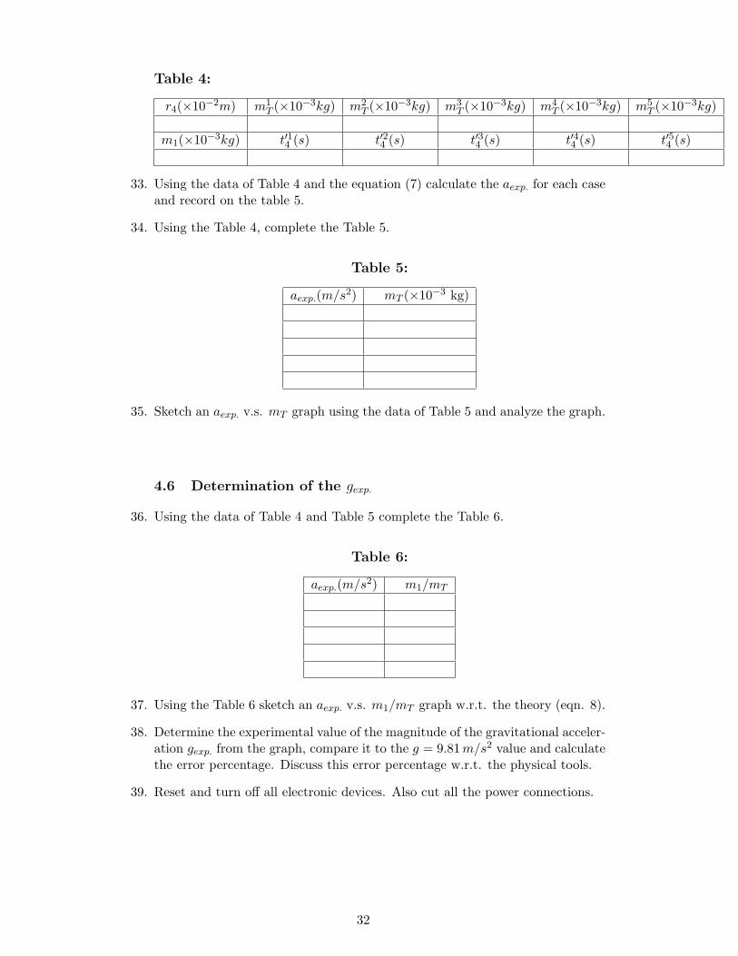
Table 4:
r4(×10−2m) m1T (×10−3kg) m2
T (×10−3kg) m3T (×10−3kg) m4
T (×10−3kg) m5T (×10−3kg)
m1(×10−3kg) t′14 (s) t′24 (s) t′34 (s) t′44 (s) t′54 (s)
33. Using the data of Table 4 and the equation (7) calculate the aexp. for each caseand record on the table 5.
34. Using the Table 4, complete the Table 5.
Table 5:
aexp.(m/s2) mT (×10−3 kg)
35. Sketch an aexp. v.s. mT graph using the data of Table 5 and analyze the graph.
4.6 Determination of the gexp.
36. Using the data of Table 4 and Table 5 complete the Table 6.
Table 6:
aexp.(m/s2) m1/mT
37. Using the Table 6 sketch an aexp. v.s. m1/mT graph w.r.t. the theory (eqn. 8).
38. Determine the experimental value of the magnitude of the gravitational acceler-ation gexp. from the graph, compare it to the g = 9.81m/s2 value and calculatethe error percentage. Discuss this error percentage w.r.t. the physical tools.
39. Reset and turn off all electronic devices. Also cut all the power connections.
32

5 Questions
1. In this experiment, the force is acting on a dynamical system which consists oftwo masses, however the magnitude of the acceleration values were determinedvia the position and time data obtained w.r.t. the motion of the one of themasses (the gliding one). Then the other calculations were performed andthe graphs were sketched according to that. How is this possible? Explainphysically.
2. Would the error percentages calculated in this experiment be higher or lower ifthe sensor 3 is used rather than the sensor 4 and why? Explain.
3. What are the ignored quantities in this experiment and in which steps of theexperiment are they ignored?
4. What are the types of data in this experiment?
33

Experiment 5Hooke’s Law
1 Purpose
To examine the Hooke’s Law by using spring(s) vertically oriented and to investigatethe harmonic behavior of the mass attached to springs in vertical direction.
1.1 Keywords
Potential energy, potential, gravitational potential, force, conserved force, harmonicmotion, simple harmonic motion, sinusoidal function, period, frequency, angular fre-quency, phase difference (phase angle).
2 Theory
According to Hooke’s Law there exists a direct relation between the force on a springand the negative variation of the position of the tip of the spring from its rest position(where there is no net force on it) and in this direct relation the constant of relationis nothing but the spring constant. In other words, if there is a force ~F (t) on a springat an instant, there is a change ∆~L(t) in the position w.r.t. the rest position of thetip of the spring in the opposite direction of that force at that instant and the springconstant k relates them s.t.
~F (t) = k (−∆~L(t))︸ ︷︷ ︸
Hooke′sLaw
(1)
If ∆~L(t), the change in the position of the tip of the spring is expressed as a gen-eral position vector ~r(t), the Hooke’s Law can be expressed in magnitudes in onedimension as;
F (t) = −kr(t) (2)
On the other hand, according to the Newton’s Second Law in magnitudes for m ≡[constant];
F (t) = ma(t) = md2r(t)dt2
(3)
Thus combining the equations (2) & (3);
md2r(t)dt2
= −k r(t) ⇒ md2r(t)dt2
+ kr(t) = 0
⇒ d2r(t)dt2
+k
mr(t) = 0 (4)
relations are obtained. The general solution of the above differential equation (4) issinusoidal functions s.t.
r(t) = A sin(ωt + φ), ω =
√k
m(5)
34

where A is the strength of r(t) (which is complex in general), ω is the angular fre-quency, & φ is the some phase difference (phase angle). However, the angular fre-quency is nothing but the ω = 2πf (where f = [frequency]) thus;
ω =
√k
m= 2πf = 2πT−1, T = [period]
hence, the period of the motion of the mass m attached to spring is as below;
T = 2π
√m
k(6)
3 Apparatus
1. Construction Apparatus (metal bar, clamp system for hanging the springs,supporting unit for ruler, tripod supporting unit for metal bar)
2. Ruler
3. Two pointer
4. Thin & thick springs. (Thin OR thick here refers to the big OR little diameterof the mathematical helixes which correspond to the springs, not refers to thediameter of the wires which the springs made of)
5. Scale
6. Various Masses (10 grams, 50 grams)
7. Chronometer
Figure 1: Experimental Setup
35

4 Procedure
4.1 Construction of the experimental Setup
1. Construct the experimental setup as in the figure using the metal bars andconnecting units.
2. Orientate the ruler in a proper way in order to have the ability of determiningthe vertical positions clearly.
4.2 Determination of the Spring Constant kthin of the ThinSpring
3. Hang the thin spring to the experimental setup.
4. Hang the scale to the lower end of the spring.
5. Determine the position of the bottom of the empty scale using the ruler andassume that position as the origin in vertical direction.
6. Add 20 grams to the hanger and determine the new vertical position of thebottom of the scale w.r.t. the origin and record the data on Table 1.
7. Add one more 20 grams to the hanger and determine the new vertical positionof the bottom of the scale w.r.t. the origin and record the data on Table 1.
8. Continue this process until the Table 1 is completed.
Table 1:
Masses Added (×10−3 kg)Vertical Positions w.r.t. the Origin (×10−2 m)
9. Calculate the magnitude of the additional force (gravitational force acting onthe additional mass OR the weight of the additional mass in this experiment)on the spring corresponding to each additional mass and record on Table 2.(Assume that |~g| = g = 9.81m/s2)
10. Using Table 1, complete the Table 2.
Table 2:
F (N) r(×10−2 m)
11. Determine the spring constant kthin using each F v.s. r couple of Table 2, thencalculate the average of those and record on Table 3 as the average experimentalvalue of the kthin.
36

Table 3:
k1thin k2
thin k3thin k4
thin k5thin kaverage
thin
12. Calculate the error percentage in kaveragethin value comparing to the theoretical
value of kthin and discuss this error percentage physically.
4.3 Determination of the Spring Constant kthick of the ThickSpring
13. Repeat exactly the procedure of the previous part (from number 3 to 12) forthick spring, however for 10 grams of additional masses for each time recordingthe data and calculations on Tables 4, 5, & 6.
Table 4:
Masses Added (×10−3kg)Vertical Positions w.r.t. the Origin (×10−2m)
Table 5:
F (N) r (×10−2m)
Table 6:
k1thick k2
thick k3thick k4
thick k5thick kaverage
thick
4.4 Determination of the Spring Constant kequivalent of the SpringSystem of Two Springs Connected in Series in Vertical Direction
14. Connect thin and thick springs in series and hang the scale to them.
15. Repeat exactly the procedure from number 3 to 12 for the spring system con-nected in series for 10 grams of additional masses for each time and record thedata and calculations on Tables 7, 8 & 9. (Calculate the equivalent spring con-stant of those two springs when they are connected in series using the theoreti-cal values of their spring constants via the relation ”k−1
equivalent ≡ k−1thin + k−1
thick”and assume that this calculated value is correct in order to determine the errorpercentage in kaverage
equivalent)
Table 7:
Masses Added (×10−3kg)Vertical Positions w.r.t. the Origin (×10−2m)
37

Table 8:
F (N) r (×10−2m)
Table 9:
k1equivalent k2
equivalent k3equivalent k4
equivalent k5equivalent kaverage
equivalent
4.5 Determination of kthin via the Graph of T 2 v.s. m
16. Hang the thin spring to the experimental setup again.
17. Measure the mass of the scale.
18. Hang the scale to the spring.
19. Add 40 grams to hanger and let it to reach its equilibrium state.
20. Record the total mass hanged on the spring (mT = mscale + madded) on Table10.
21. Determine the vertical equilibrium position of the hanger.
22. Expand the spring by taking the hanger downwards sligthly (be careful aboutnot to expand the spring too much) from the equilibrium point determinedabove.
23. Release the hanger, start the chronometer and start to count complete harmoniccycles at the same instant.
24. Count the number of five complete harmonic cycles and stop the chronometer.
25. Record the time t required for the five complete harmonic cyles on Table 10.
26. Add one more 40 grams to the hanger and repeat the procedure for new mT
value from number 20 to 25.
27. Continue this process until the first two rows of the Table 10 is completed.
28. Calculate the period values and record on Table 10.
29. Calculate the squares of the period values and record on Table 10.
38

Table 10:
mT (×10−3kg)t (s)T (s)T2(s2)
30. Sketch a T 2 v.s. m graph using the data of Table 10 by calculating the co-ordinates of all data points of the graph w.r.t. the scalings of the graph axes(Express all results and at least one calculation of coordinate explicitly) anddetermine the kthin by means of the graph.
31. Calculate the error percentage in kthin value comparing to the theoretical valueof kthin and discuss this error percentage physically.
32. Remove the thin spring and the scale from the experimental setup.
4.6 Determination of kthick via the Graph of T 2 v.s. m
33. Hang the thick spring to the experimental setup.
34. Hang the scale to the thick spring.
35. Repeat the procedure for thick spring from number 19 to 32 for additional 10grams recording the data and calculations on Table 11.
Table 11:
mT (×10−3kg)t (s)T (s)T2(s2)
5 Questions
1. Are there any ignored physical quantity in this experiment or not? If there are,what are they and in which part(s) of the experiment are they ignored, explain.
2. Does the connection order of the springs in the springs in series part of thisexperiment matter, OR not? Why OR why not?
3. Of course the motion of the mass in the period part of this experiment is notan exactly simple harmonic motion in practice. Why, explain. However, is itan exactly simple harmonic motion theoretically OR not? Explain.
4. What must be expected in the period part of this experiment if it is performedin water in the existence of a gravitational field, in free space (where there is nopotential on the mass) and in an elevator moving downwards with an increasingspeed. Explain respectively.
5. What are the types of data in this experiment?
39

Experiment 6Ballistic Pendulum and Conservation of Energy
1 Purpose
To determine the initial speed of a ball in terms of the momentum conservation atthe instant of collision and the conservation of mechanical energy after the collisionusing the ballistic pendulum apparatus.
1.1 Keywords
Energy, kinetic energy, potential energy, conservation of energy, momentum, conser-vation of momentum, collision, elastic collision, inelastic collision.
2 Theory
One of the most important principles in physics is the concept that total energy ofa system is always conserved. The energy can change form but the sum of all ofthese forms of energy must stay constant unless energy is added or removed from thesystem.
Another important conserved quantity is momentum. The principle of conservationof momentum states that the total momentum of a system remains constant if thereis no external force. Collision processes are good examples of this concept. There aretwo types of collision named elastic and inelastic collision. An elastic collision betweentwo objects is one in which the total kinetic energy (as well as total momentum) ofthe system is the same before and after the collision. Collisions between billiard ballsare only approximately elastic because some deformation and loss of kinetic energytake place. A collision in which the total kinetic energy after the collision is lessthan before the collision is called an inelastic collision. A special type of inelasticcollision in which the colliding bodies stick together and move as one body after thecollision is often called a completely inelastic collision. The most common examplefor completely inelastic collision is the ballistic pendulum. The ballistic pendulum isan apparatus used to measure the speed of a fast-moving projectile, such as a bullet.
In this laboratory we will use a ballistic pendulum to measure the speed of a ballprojected by a spring gun. Figure 6.1 shows a ball of mass m moving initially in thehorizontal direction with speed v0x that then strikes a pendulum designed to catchthe ball. The pendulum of mass M catches the ball and swings about pivot pointO to some maximum height y2 above its original height y1. The system of ball pluspendulum rises a vertical distance of ∆y = y2 − y1 as a result of the process.
Momentum is conserved because the external net force on the system at the instantof the collision is zero. The two particles stick together after the collision and movewith the same velocity.
The equation for conservation of momentum is;
mv0x = (m + M)V (1)
40

Figure 1: Ballistic Pendulum
If we assume that the potential energy of the pendulum at its resting position is zero,the following is valid for the potential energy at the highest point of the oscillation:
Epot = (m + M)g∆y
where g is the magnitude of the gravitational acceleration and ∆y the height by whichthe centre of gravity was raised. In Figure 6.1 one sees that with r as the distancebetween the pivot point and the centre of gravity, one can also write this formula as:
Epot = (m + M)gr(1− cos(φ))
This potential energy must be equal to the kinetic energy Ekin immediately after thecollision:
Ekin =12(m + M)V 2 (2)
If one substitutes the momentum p = (m + M)V in this equation, the following isobtained:
Ekin =p2
2(m + M)OR p =
√2(m + M)Ekin
before the collision the pendulum was at rest. Due to the principle of conservation ofmomentum, the momentum p = mv must be equal in magnitude to the momentumof the ball before the collision. One obtains the following for the speed v of the ballbefore the start, for the parameter to be determined:
v =m + M
m
√2gr(1− cos(φ)) (3)
This equation shows the function v(φ). For the evaluation, determine the mass of theball. The position of the center of gravity with captured steel ball is marked on thependulums body. The mass of the pendulums body can only be determined togetherwith its mounting.
41

3 Apparatus
1. Ballistic unit
2. Ballistic pendulum
3. Speed measuring attachment
4. Steel ball
5. Wooden ball
4 Procedure
Figure 2: Experimental Setup
1. The experimental setup must be standing on a stable table during the measure-ments.
2. Before stretching the spring of the throwing device, affix the steel ball to theholding magnet on the bolt.
3. Then pull the bolt back until the desired lock-in position has been reached.There are three levels. Pull the bolt until the first level.
4. Now ensure that the pendulum is at rest and that the trailing pointer indicatesnearly zero.
5. After these preparations have been completed, trigger the shot by pulling therelease lever.
6. Record speed of the ball from the speed measuring attachment every time youpull the release lever.
7. Read the amplitude of the pendulum’s oscillation from the trailing pointer.8. Due to the friction involved in the functioning of the trailing pointer, the mea-
sured amplitude may be slightly low. Because of that repeat the experiment for asecond and a third time without resetting the trailing pointer. When the trailingpointer is not moved any further, one can assume that the angle indicated has notbeen falsified by friction.
42

9. Do the experiment again for the second and third level of the unit and fill inthe Table 6.1.
10. Measure the mass of steel ball and wooden ball. Here the mass M is M =122× 10−3kg.
11. Measure the length of the ballistic pendulum (r).
Table 6.1:
... v (m/s) φ (degree)1st level of the starter unit2nd level of the starter unit3rd level of the starter unit
12. Calculate the experimental speed of the ball with formula (3) and comparethe result with the one you obtained from speed measuring attachment. Find thepercentage error.
13. Do the experiment again for the wooden ball and record the data to the Table6.2.
Table 6.2:
... v (m/s) φ (degree)1st level of the starter unit2nd level of the starter unit3rd level of the starter unit
14. Plot vexp versus φ for steel and wooden balls respectively.
5 Questions
1. What are the conditions under which the total momentum of a system is con-served?
2. Is the case that two objects collide and stick together an elastic or inelasticcollision?
3. How many types of collisions are there?
6 References
1. Serway R. A., Beichner R. J., Jewett J. W. Physics for Scientists and Engineers,Brooks Cole, U.S., 2000
2. Young H. D., Freedman R. A. Sears and Zemansky’s University Physics:WithModern Physics , Pearson Addison-Wesley, U.S., 2008
43
Experiment 7Conservation of Momentum/Laws of Collision
1 Purpose
1. To understand the conservation of linear momentum.
2. To investigate whether or not momentum and energy are conserved in elasticand inelastic collisions.
Keywords: Momentum, kinetic energy, elastic-inelastic collision, conservation ofmomentum, conservation of energy.
2 Theory
The momentum ~p of an object is the product of its mass and its velocity:
−→p = m−→v (1)
Momentum is a vector quantity, because it is multiplication of velocity (a vector)and mass (a scalar).
Newton originally stated his second law using momentum, rather than acceleration:
−→F net =
d−→pdt
(2)
where
−→F net =
N∑
i=1
−→F i =
−→F 1 +
−→F 2 +
−→F 3... +
−→F N (3)
Here−→F i’s show all the forces that act on an object and
−→F net is vector sum of
all these forces. In the case we are considering, namely where there are no externalforces, the above equation reads;
d−→pdt
= 0 or −→p = constant (4)
which states that the linear momentum of a system is conserved, when the net ex-ternal force is zero.
If the system consists of two or more particles, the total momentum is the vectorsum of the individual particles. That is if there are m particles in the system thetotal momentum is
−→p tot =m∑
i=1
−→p i = −→p 1 +−→p 2 +−→p 3... +−→p m. (5)
The equation ?? becomes
44

d−→p tot
dt= 0 (6)
for this case.Consider a collision between two objects (object 1 and object 2). For such a
collision, the time interval that we are most interested in is the period just before thecollision to just after the collision. The forces acting between the two objects in thistime interval are equal in magnitude and opposite in direction (Newton’s third law):
−→F 12 = −−→F 21. (7)
So if there is no frictional force, the net force will be zero on the system andmomentum will be conserved. Therefore, we can write the law of conservation ofmomentum as follows;
−→p initial = −→p final (8)
Despite their fundamental nature, the conservation laws are often difficult to ob-serve in ordinary experiences, primarily because of the presence of friction. Frictionbetween moving bodies and their surroundings means there are external forces act-ing on the system, therefore, the conservation laws do not apply. So, to observe theconservation laws, friction must be eliminated as much as possible.
In this experiment, we will examine two types of collisions: elastic collisions, inwhich energy is ideally conserved, and inelastic collisions, in which energy of thesystem is not conserved. However, linear momentum is ideally conserved for bothtypes of collisions.
In elastic collisions the objects bounce off each other without losing any energy.For a system composed of two masses along a track, we can write conservation ofmomentum and energy as follows :
m1−→v 1i + m2
−→v 2i = m1−→v 1f + m2
−→v 2f (conservation of momentum) (9)
12m1v
21i +
12m2v
22i =
12m1v
21f +
12m2v
22f (conservation of energy) (10)
A collision is completely inelastic when the bodies stick together after a collision.An inelastic collision is one in which part of the kinetic energy is changed to someother form of energy in the collision. Any macroscopic collision between objects willconvert some of the kinetic energy into internal energy and other forms of energy, sono large scale impacts are perfectly elastic. We can write conservation of momentumfor a totally inelastic collision as follows :
m1−→v 1i + m2
−→v 2i = (m1 + m2)−→v (conservation of momentum) (11)
The laws of conservation of energy and momentum are among the most fundamen-tal and useful laws of physics
45

3 Apparatus
1. Demonstration Track, magnet with plug for starter system , low friction sap-phire bearing
2. Starter system for motion track
3. Needle with plug, Tube with plug
4. Carts
5. Light barrier
6. Timer
7. Shutter plates for low friction cart
4 Procedure
Part A : Elastic Collision
1. Align the track horizontally. Be careful about that the track is precisely aligned.
2. Position the starter system at the left end of the track. Please note that, inorder to start the cart with an initial momentum, the starter system must beinstalled so that the cart receives an impulse from the ram of the starter system(Fig. 1)
3. Attach a plasticine-filled tube to the end holder at the right-hand end of thetrack in order to stop the cart without a strong impact (Fig. 2).
4. Position the three light barriers at the 50 cm, 70 cm and 90 cm marks on thetrack.
5. Connect light barriers to the sockets in field “1”,“2”,“3” of the timer. Connectthe yellow sockets of the light barriers to the yellow sockets of the measuringinstrument, the red sockets to their red counterparts, and the blue sockets ofthe light barriers to the white sockets of the timer (see Fig.3)
6. Place the two carts on the track. Equip the cart on the left, which is closerto the starter system with a magnet with a plug facing the starter system andwith a tube with a plug in the direction of motion. Place the second cart at73cm mark on track.
7. Fasten a shutter plate (x = 100mm) in both carts.
8. Set the timer to mode 1.
9. Determine the masses of carts by way of the balance.
10. Prior to every collision experiment, press the ”Reset” button in order to resetthe displays.
11. Cart 1 will be accelerated by the starter system and cart 2 will be stationaryat 73cm mark.
46

12. After the collision, the light barrier in the direction of motion of both carts willbe interrupted. It will only register the shading time of the shutter plate.
13. Use the shading times ti and the shutter plate length x = 100mm to determinethe velocities vi = x/ti. Since the velocities are vector quantities, their sign isimportant.
14. Record the measuring times five times and take the mean of these values. Then,repeat the measurement for different cart masses and mass ratios.
15. Calculate the momentum and energy values before and after collision by usingequation 7 and 8.
16. Compare the values and make comments about it.
Figure 1: Starter system for providing the necessary impulse
Figure 2: End holder with plasticine
47

Figure 3: Connection of the light barriers
Table 1:
v2i = 0masses (kg) t1 (s) t2 (s) t3 (s) t1 (s) t2 (s) t3 (s) v1i (m
s ) v1f (ms ) v2f (m
s )m1 =m2 =
m1 + 20 =
m2 =m1 + 40 =
m2 =m1 + 60 =
m2 =
masses (kg) P1i (kgms ) P1f (kgm
s ) P2f (kgms ) E1i (J) E1f (J) E2f (J)
m1 and m2
m1 + 20 and m2
m1 + 40 and m2
m1 + 60 and m2
Part B : Inelastic Collision
1. Perform same steps in part A. Only the following points are different from part
48

A:
2. This time position two light barriers at 50 cm and 90 cm marks on the track.
3. Equip the cart on the left, which is closer to the starter system with a needlewith plug facing the other cart. Equip the cart on the right with plasticine-filledtube facing the other cart at 73cm mark on track.
4. Calculate the momentum and energy values before and after collision by usingequation 8 and 9.
5. Compare the values and comment about it.
Table 2:
v2i = 0masses (kg) t1 (s) t2 (s) t1 (s) t2 (s) v1i (m
s ) vf (ms )
m1 =m2 =
masses (kg) P1i (kgms ) Pf (kgm
s ) E1i (J) Ef (J)m1 and m2
5 Questions
1. A 0.112 kg ball moving at 154 cm/s strikes a second ball of the same massmoving in the opposite direction at 46 cm/s. The second ball rebounds andtravels at 72 cm/s after the head on collision. Determine the post-collisionvelocity of the first ball.
2. A 3000 kg truck moving rightward with a speed of 20 m/s collides head-on witha 1000 kg car moving leftward with a speed of 40 m/s. The two vehicles sticktogether and move with the same velocity after the collision. Determine thepost collision velocity of the car and truck.
3. A bicycle has a momentum of 24 kgm/s. What momentum would the bicyclehave if it had twice the mass and was moving at the same speed?
4. A 0.150-kg baseball moving at a speed of 45.0 m/s crosses the plate and strikesthe 0.250-kg catcher’s mitt (originally at rest). The catcher’s mitt immediatelyrecoils backwards (at the same speed as the ball) before the catcher applies anexternal force to stop its momentum. If the catcher’s hand is in a relaxed stateat the time of the collision, it can be assumed that no net external force existsand the law of momentum conservation applies to the baseball-catcher’s mittcollision. Determine the post-collision velocity of the mitt and ball.
6 References
1. Phywe Physics Laboratory Manual
49

Experiment 8Mechanical Conservation of Energy (Maxwell’s
Wheel)
1 Purpose
To measure the moment o inertia of Maxwell’s wheel and to determine the potentialenergy, the energy of translation and the energy of rotation as a function of time byusing the Maxwell’s wheel.
1.1 Keywords
The conservation of energy, energy of translation, energy of rotation, potential energy,moment of inertia, angular velocity, angular acceleration.
2 Theory
According to the conservation of mechanical energy, if the forces acting on the systemare conservative, the total mechanical energy of a system remains constant.
∆Ek + ∆Ep = 0. (1)
The total kinetic energy of an object which is in rolling motion is the sum of thetranslational kinetic energy of its center of mass and the rotational kinetic energy ofthe body.
Ek = Et + Er (2)
where
Et =12mv2 (3)
and
Er =12Iω2. (4)
The total energy E of the Maxwell disk, of mass m and moment of inertia Iz aboutthe axis of rotation, is composed of the potential energy Ep, the energy of translationEt and the energy of rotation Er:
Etotal = Ep + Et + Er (5)
and thenE = m~g~s +
12m~v2 +
12Iz~ω
2 (6)
Here, ~ω denotes the angular velocity, ~v the translational velocity, ~g the accelerationdue to gravity and ~s the (negative) height.
Using the notation of Fig. 8.1,
50

Figure 1: Relationship between the increase in angle dφ and the decrease in heightd~s in the Maxwell disk.
|d~s| = |d~φ||~r| (7)
and
|~v| = |d~sdt| = |d
~φ
dt|~r = |~ω|~r (8)
where r is the radius of the spindle. In the present case ~g is parallel to ~s and ~ω isperpendicular to ~r so that one obtains.
E = −mgs(t) +12(m +
Iz
r2)(v(t))2. (9)
Since the total energy E is constant with respect to time, differentiation gives
0 = −mgv(t) + (m +Iz
r2)v(t)v′(t) (10)
then
0 = −mg + (m + Iz/r2)d2s(t)dt2
⇒ d2s(t)dt2
=mg
m + Iz/r2
⇒ d
dt
ds(t)dt
=mg
m + Iz/r2
⇒∫
d(ds(t)dt
) =∫
(mg
m + Iz/r2)dt
⇒ ds(t)dt
=mg
m + Iz/r2t + k1
For v(t = 0) = 0 k1 = 0 and one gets;
v(t) =ds
dt=
mg
(m + Izr2 )
t (11)
51

When we integrate the equation ??,∫
ds =∫
mg
m + Izr2
tdt (12)
We obtain;
s(t) =12
mg
(m + Izr2 )
t2 + k2 (13)
For s(t = 0) = 0, k2 = 0 and
s(t) =12
mg
(m + Izr2 )
t2 (14)
is obtained. In the experiment the mass m is m=0,470 kg and the radius r of thespindle is r = 2.510−3m.
3 Apparatus
1. Maxwell’s wheel
2. Light barrier with counter
3. Holding device w. cable release
4. Meter scale
5. Power supply 5 V DC/2.4 A with 4 mm plugs
6. Capacitor 100 nF
4 Procedure
1. The experimental set up is as shown in Fig. 8.2. By using the adjusting screw onthe support rod, the axis of the Maxwell disk is aligned horizontally in the unwoundcondition. When winding up, the windings must run inwards.
2. The winding density should be equal on both sides. It is essential to watch thefirst up and down movements of the disk. Furthermore, the cord should always bewound in the same direction at start.
3. To measure the falling time of the wheel, wind the cord until the wheel reachthe height determined in Table 8.1.
4. Press the wire cable release and lock it.5. Adjust the light barrier to the mode 3 using the selection button on it.6. Press the ”set” button of the light barrier in order to reset it.7. Start the motion of the wheel and the counter of the light barrier by setting the
wire cable release free and pressing it again instantly, and keep the wire cable releasepressed until the motion finishes.
8. Record the time value t(s) on Table 8.1.9. At this point adjust the light barrier to the mode 2 and remove the blue cable
from wire cable release apparatus.
52

Figure 2: Experimental Setup
10. To measure the ∆t value elevate the wheel to the starting position again andfix it by pressing the wire cable release.
11. Set the wire cable release free and start the motion of the wheel again.12. After the motion has completed, record the new time value ∆t which is the
time required for the thin metal rod of the wheel passes through the light barrier.13. Calculate the translational velocity of the disc at the bottom point of the
motion by using v = 2r/∆t equation.14. Using the Table 8.1 sketch an s(t2) and v(t) graph.15. Determine the experimental value of moment of inertia Iz of the wheel from
the slope of s v.s. (t2) the graph.16. Calculate the potential energy, the translational kinetic energy, and the rota-
tional kinetic energy of the Maxwell’s wheel and record them on Table 8.2.17. Plot Ep v.s. t, Et v.s. t and Er v.s. t graphs. Is the mechanical energy
conserved? Make comments especially on the energy conservation and on the graphs.
Table 8.1
s (m) t (s) t2 (s2) v (m/s) ∆t(s)0,100,200,300,400,50
53

Table 8.2
s (m) Ep (J) Et (J) Er (J)0,100,200,300,400,50
5 Questions
1. If we use a plate square in shape rather than disk in the experiment with asame moment of inertia do you expect any difference in the experiment or not?Why? Explain.
2. Is it possible to change the translational kinetic energy of an object withoutchanging its rotational energy?
3. Is the energy conserved if the mass of the disk increases continuously duringthe motion?
54