Embed Size (px)
Citation preview
ADVANCED ASTROPHYSICS
This book develops the basic underlying physics required for a fuller, richer under-standing of the science of astrophysics and the important astronomical phenomenait describes. The Cosmos manifests phenomena in which physics can appear inits most extreme, and therefore more insightful, forms. A proper understanding ofphenomena such as black holes, quasars and extrasolar planets requires that weunderstand the physics that underlies all of astrophysics. Consequently, developingastrophysical concepts from fundamental physics has the potential to achieve twogoals: to derive a better understanding of astrophysical phenomena from first prin-ciples and to illuminate the physics from which the astrophysics is developed. Tothat end, astrophysical topics are grouped according to the relevant areas of physics.The book is ideal as a text for graduate students and as a reference for establishedresearchers.
The author obtained his PhD in 1984 from the University of Toronto where heearned the Royal Astronomical Society of Canada Gold Medal for academic ex-cellence. After a brief postdoctoral stint at the University of British Columbia, hejoined the faculty at the University of New Mexico where he pursued his interests inradio astronomy. He has been teaching for the past 17 years, earning an “excellencein teaching” award for the graduate courses on which this book is based. Dr. Durichas over 100 scientific publications and has authored and/or edited five books. Inaddition, he has developed a number of online classes, including a completely inter-active, web-based freshman astronomy course. He is the recipient of the “Regent’sFellowship”, the highest honour that UNM bestows on its faculty. His researchhas taken him around the world to over a dozen countries, accounting in part, forthe global perspective that characterizes his book. Dr. Duric is a member of theAmerican Astronomical Society and the Canadian Astronomical Society.


ADVANCED ASTROPHYSICS
NEB DURICUniversity of New Mexico

Cambridge, New York, Melbourne, Madrid, Cape Town, Singapore, São Paulo
Cambridge University PressThe Edinburgh Building, Cambridge , United Kingdom
First published in print format
- ----
- ----
- ----
© Neb Duric 2004
2003
Information on this title: www.cambridge.org/9780521819671
This book is in copyright. Subject to statutory exception and to the provision ofrelevant collective licensing agreements, no reproduction of any part may take placewithout the written permission of Cambridge University Press.
- ---
- ---
- ---
Cambridge University Press has no responsibility for the persistence or accuracy ofs for external or third-party internet websites referred to in this book, and does notguarantee that any content on such websites is, or will remain, accurate or appropriate.
Published in the United States of America by Cambridge University Press, New York
www.cambridge.org
hardback
paperbackpaperback
eBook (NetLibrary)eBook (NetLibrary)
hardback

Contents
Preface page xiiiPart I Classical mechanics 11 Orbital mechanics 3
1.1 Universal gravitation 31.1.1 Center of mass 31.1.2 Reduced mass 4
1.2 Kepler’s laws 51.2.1 Planetary orbits 9
1.3 Binary stars 111.3.1 Visual binaries 111.3.2 The apparent orbit 111.3.3 The true orbit 121.3.4 Determining the orbital elements 141.3.5 Spectroscopic binaries 141.3.6 The mass function 171.3.7 Summary of binary star studies 181.3.8 Mass–luminosity relation 19
1.4 Extrasolar planets 201.4.1 The astrometric method 211.4.2 The radial velocity method 221.4.3 The transit method 24
1.5 References 251.6 Further reading 25
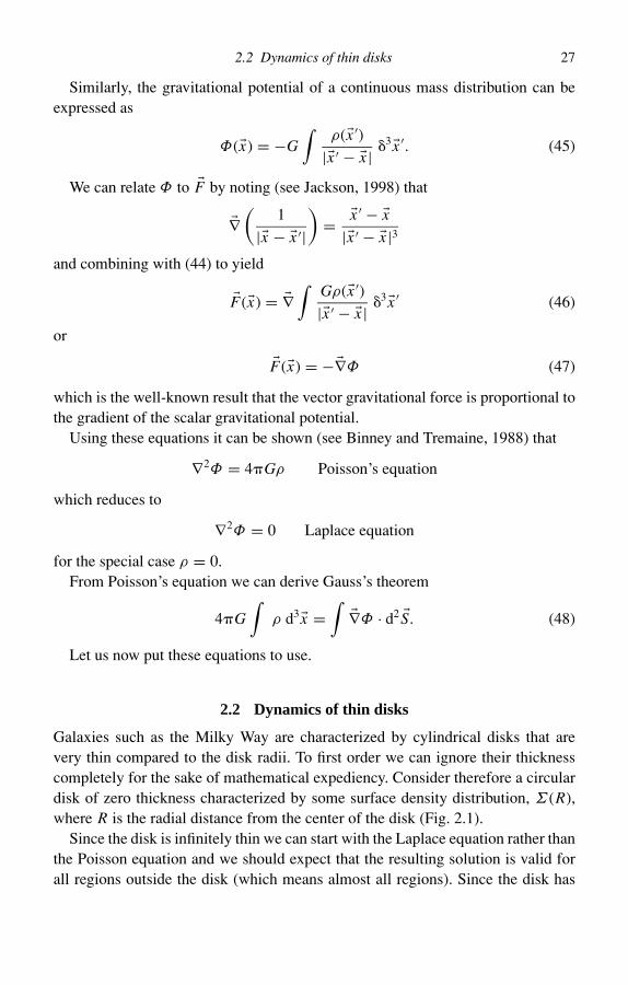
2 Galaxy dynamics 262.1 Potentials of arbitrary matter distributions 262.2 Dynamics of thin disks 27
v

vi Contents
2.3 Rotation curves of disk galaxies 302.3.1 Rotation curves of real spiral galaxies 31
2.4 N-body gravitational systems 342.4.1 Equation of motion 342.4.2 The Virial theorem 352.4.3 Clusters of galaxies 36
2.5 References 392.6 Further reading 39
3 Cosmic expansion and large scale structure 403.1 The expansion of the Universe 40
3.1.1 The cosmological constant 423.2 Large-scale cosmic structure 45
3.2.1 Overview 453.2.2 Correlation functions of galaxies 463.2.3 Dark matter and large-scale structure 473.2.4 Hot and cold dark matter 513.2.5 The Jeans’ mass and gravitational stability 523.2.6 Possible models of structure formation 54
3.3 References 553.4 Further reading 55
Part II Statistical mechanics 574 Overview of statistical mechanics 59
4.1 Thermodynamics 594.2 Classical statistical mechanics 614.3 Quantum statistical mechanics 63
4.3.1 Bose–Einstein statistics 644.3.2 Fermi–Dirac statistics 64
4.4 Photon distribution function 654.5 Thermodynamic equilibrium 664.6 Further reading 68
5 The early Universe 695.1 The 3 K background radiation 69
5.1.1 History of the background radiation 695.1.2 Evolution of energy density 70
5.2 Galaxy formation 715.3 Local cosmology and nucleosynthesis 72
5.3.1 Overview 725.3.2 Primordial helium 73
5.4 Reaction rates 755.4.1 Introduction 75

Contents vii
5.4.2 Barrier penetration 775.4.3 Estimating reaction rates 815.4.4 Destruction of D 825.4.5 Formation of D 825.4.6 Formation of 4He 83
5.5 Particle equilibria in the early Universe 835.5.1 Overview 835.5.2 Chemical equilibrium 865.5.3 The early Universe 875.5.4 The neutron–proton ratio 875.5.5 Reaction freeze-out 885.5.6 Reaction timescale 905.5.7 Formation of deuterium 91
5.6 Further reading 936 Stellar structure and compact stars 94
6.1 Hydrostatic equilibrium 946.2 Fermion degeneracy 97
6.2.1 White dwarf equation of state 1006.2.2 Mass–radius relation for white dwarfs 100
6.3 Internal structure of white dwarfs 1006.3.1 Relationship between pressure and
energy density 1016.3.2 Relating electron number density to the
mass density 1046.3.3 Other sources of pressure 1056.3.4 Equation of state 1056.3.5 Internal structure of white dwarfs 1056.3.6 Estimating the radius and mass of a
white dwarf 1076.4 Stability of compact stars 109
6.4.1 Total energy 1096.4.2 Electron capture 1106.4.3 Maximum density 111
6.5 Structure of neutron stars 1146.5.1 Overview 1146.5.2 Liquid layer 1156.5.3 The crust 1176.5.4 The core 119
6.6 Pulsars 1196.7 Further reading 121

viii Contents
Part III Electromagnetism 1237 Radiation from accelerating charges 125
7.1 The Lienard–Wiechert potential 1257.1.1 Scalar and vector potentials 1257.1.2 Green’s function solution 1267.1.3 The L–W potentials 127
7.2 Electric and magnetic fields of a moving charge 1287.2.1 Moving charge at constant velocity 1297.2.2 Radiation from accelerating charges – the far zone 1317.2.3 Angular distribution of radiation 1317.2.4 Total emitted power 133
7.3 Further reading 1348 Bremsstrahlung and synchrotron radiation 135
8.1 Bremsstrahlung 1358.1.1 Single particle collisions 1358.1.2 Radiation from an ensemble of particles 137
8.2 Synchrotron radiation 1388.2.1 Total power 1398.2.2 The received spectrum 1408.2.3 Spectrum of a power-law energy distribution 141
8.3 Further reading 1439 High energy processes in astrophysics 144
9.1 Neutron stars 1449.2 Supernova remnants 145
9.2.1 Particle acceleration 1459.3 Radio galaxies 1489.4 Galactic X-ray sources 152
9.4.1 The energy source 1539.4.2 Maximum luminosity/Eddington limit 1539.4.3 Characteristic temperature 1549.4.4 Mass transfer 154
9.5 Accretion disks 1549.5.1 Disk hydrodynamics 1569.5.2 The emission spectrum of the disk 157
9.6 Pulsars revisited 1599.6.1 The radiation field 1609.6.2 Radiated power 1619.6.3 The Braking Index 1629.6.4 The static magnetic field 1629.6.5 The static electric field 162

Contents ix
9.7 Reference 1639.8 Further reading 163
10 Electromagnetic wave propagation 16410.1 EM waves in an un-magnetized plasma 165
10.1.1 Dispersion measure 16610.2 EM waves in a magnetized medium 167
10.2.1 Rotation measure 17010.3 Reference 17210.4 Further reading 172
Part IV Quantum mechanics 17311 The hydrogen atom 175
11.1 Structure of the hydrogen atom 17511.1.1 Case 1 r → ∞ 17711.1.2 Case 2 r → 0 17711.1.3 What about the in-between? 17811.1.4 Normalizing R(r ) 179
11.2 Total wave function 18111.3 Probability functions 18111.4 Energy eigenstates and transitions 18511.5 Further reading 185
12 The interaction of radiation with matter 18712.1 Non-relativistic treatment 18712.2 Single particle Hamiltonian 18812.3 Separation of static and radiation fields 189
12.3.1 Relative importance of H0, H1 and H2 18912.4 Radiative transitions 190
12.4.1 Semi-classical approach 19012.4.2 The Hamiltonian of the radiation field 19112.4.3 The perturbation Hamiltonian 19212.4.4 Time-dependent perturbation theory 193
12.5 Absorption of photons 19412.5.1 Absorption cross-sections 19612.5.2 Dipole transition probability 19712.5.3 Bound–bound absorption cross-section 198
12.6 Spontaneous emission 19912.7 Photoionization 200
12.7.1 Bound–free cross-sections 20212.8 Selection rules 203
12.8.1 Dipole selection rules 20412.8.2 Electric quadrupole transitions 205

x Contents
12.9 Numerical evaluation of transition probabilities 20612.9.1 The Lyman transition 20712.9.2 Bound–free absorption cross-section 209
12.10 HII regions 21012.10.1 Ionizing stars 211
12.11 Ionization of a pure hydrogen nebula 21212.11.1 Radius of HII region 216
12.12 Quasars and the Lyman forest 21612.12.1 Correlation studies 21812.12.2 Column density of the HI responsible for
the Ly- forest 22012.13 Reference 22012.14 Further reading 221
13 Atomic fine structure lines 22213.1 Electron spin 222
13.1.1 Relativistic Hamiltonian 22213.2 Dirac’s postulate 223
13.2.1 The Dirac equation 22413.2.2 Free particle at rest 22413.2.3 Non-relativistic limit of Dirac’s
equation 22513.3 Radiative transitions involving spin 227
13.3.1 Zeeman effect 22813.4 Relativistic correction with A = 0 22813.5 Atomic fine structure 229
13.5.1 Spin–orbit interaction 23013.5.2 Time-independent perturbation theory 23013.5.3 The jm representation 23113.5.4 Solution for ESO 232
13.6 Further reading 23414 Atomic hyperfine lines 235
14.1 The 21 cm line of hydrogen 23514.1.1 Transition rate 23814.1.2 The 21 cm line profile 239
14.2 The Doppler effect 24014.2.1 Doppler broadening of the 21 cm line 241
14.3 Neutral hydrogen in galaxies 24214.3.1 Equation of transfer for HI emission 24214.3.2 Emission or absorption? 244

Contents xi
14.4 Measuring HI in external galaxies 24414.4.1 Integral properties of galaxies 24514.4.2 Kinematics of the HI 245
14.5 Probing galactic mass distributions 24614.5.1 HI rotation curves 247
14.6 References 25314.7 Further reading 253
15 Transitions involving multi-electron atoms 25415.1 Symmetry of multi-particle wave functions 25415.2 The helium atom 255
15.2.1 The ground state 25515.2.2 Lowest excited states 25715.2.3 Summary 258
15.3 Many-electron atoms 25915.3.1 The Hartree–Fock procedure 260
15.4 Forbidden lines in astrophysics 26115.4.1 Collisional equilibria 26115.4.2 Line emission and cooling of nebulas 26315.4.3 Statistical equilibrium for N levels 26515.4.4 OIII lines as probes of temperature 26615.4.5 Line ratios as density probes 26915.4.6 Observations of nebulas 27015.4.7 Observations of active galactic nuclei 270
15.5 Further reading 27216 Molecular lines in astrophysics 273
16.1 Diatomic molecules 27316.1.1 Inter-nuclear potential 27316.1.2 Electronic transitions 27316.1.3 Vibrational transitions 27416.1.4 Rotational transitions 27416.1.5 Summary 275
16.2 Diatomic molecules with two valence electrons 27516.2.1 The Born–Oppenheimer Approximation 276
16.3 Translational and internal degrees of freedom 27816.3.1 Vibrations and rotations 27916.3.2 Vibrations – harmonic oscillator approximation 280
16.4 Dipole transition probability 28116.4.1 Pure rotational spectra 282
16.5 Transitions between vibrational levels 283

xii Contents
16.6 Transitions between electronic levels 28416.7 The H2 molecule 28516.8 The CO molecule 28716.9 Other molecules 29016.10 Life in the Universe 291
16.10.1 The building blocks of life 29116.10.2 Communicating with other civilizations 293
16.11 Further reading 293Index 294

Preface
Astrophysics strives to describe the Universe through the application of fundamen-tal physics. The Cosmos manifests phenomena in which the physics can appear inits most extreme, and therefore more insightful, forms. Consequently, developingastrophysical concepts from fundamental physics has the potential to achieve twogoals: to derive a better understanding of astrophysical phenomena from first prin-ciples, and to illuminate the physics from which the astrophysics is developed. Tothat end, astrophysical topics are grouped, in this book, according to the relevantareas of physics. For example, the derivation of the laws of orbital motion, used inthe detection of extrasolar planets, takes place in the classical mechanics part of thebook while the derivation of transition rates for the 21 cm neutral hydrogen line,used to probe galaxy kinematics, is performed in the quantum mechanics part. Thebook could serve as a text for graduate students and as a reference for establishedresearchers.
The content of this book is based on the material used by the author in supportof advanced astrophysics courses taught at the University of New Mexico. Theintended audience consists of graduate students and senior undergraduates pur-suing degrees in physics and/or astrophysics. Perhaps the most directly relevantdemographic is the combined Physics and Astronomy departments. These depart-ments tend to emphasize the fundamental physics regardless of the research trackpursued by the student. In many cases a separate astrophysics degree is not anoption. In these departments (such as the author’s) all students must pass the samephysics comprehensive examination. Consequently, students must be well preparedin fundamental physics both from the points of view of course work as well as re-search. In the latter case a strong physics foundation is very helpful in developingthesis topics to an acceptable level in a physics-dominated department. This bookis specifically aimed at those departments.
The department of Physics and Astronomy at the University of New Mexicorequires its graduate students to take the physics comprehensive exam. Courses
xiii

xiv Preface
based on the material in this book have helped astrophysics and physics studentsprepare for these exams. I attribute this benefit to the fact that the astrophysicaltopics provide interesting and insightful manifestations of the fundamental physics,of which, the students previously may have had only a theoretical knowledge. Itherefore expect the book to impact the physics as well as the astrophysics studentsin the mixed departments. I also expect that graduate students in physics-only andastronomy-only departments may choose to use this book to hone their researchskills. Targeting junior/senior undergraduates is also possible in schools where thescience curricula are robust.
Multi-disciplinary and cross-disciplinary investigations are playing an increas-ingly important role in scientific research. The cross-over of particle physicists intocosmology, and the establishment of the field of astroparticle physics, is just onemanifestation of the growing overlap between physics and astrophysics disciplines.The emphasis on the linkage of fundamental physics and astrophysics makes thisbook potentially useful as a reference to physics and astrophysics researchers whowish to broaden their research base.
The author acknowledges the help of Dr. Rich Epstein (Los Alamos NationalLaboratory) who co-taught the first course in the series of courses that have led to thedevelopment of the material used in this book. The cooperation and help of the manystudents who have taken these courses has been instrumental in identifying manytypos and inconsistencies in the course material. Finally, the author acknowledgesthe help and support of the department of physics and astronomy at UNM and thepatience and encouragement of family and friends in this endeavor.

Part I
Classical mechanics
The visible Universe contains hundreds of billions of galaxies, each consisting ofbillions of stars. Recent discoveries of extrasolar planets lead us to believe thata typical galaxy may contain billions of planets (and presumably, asteroids andcomets). The planets, stars and galaxies interact on a hierarchy of scales rangingfrom AU to parsec to megaparsec, experiencing forces arising from gravity, on allscales, and cosmic expansion on the larger scales. The combination of gravitationalattraction and cosmic expansion has shaped the visible matter in the Universe intoa hierarchy of structures leading to clusters and superclusters of galaxies.
A full description of the interactions that define the large-scale structure of theUniverse and its constituent parts requires the application of general relativity onall scales and the introduction of a new force, as embodied in the recently proposedcosmological constant, on the largest scales. In this part, however, we limit ourselveslargely to the application of classical (Newtonian) mechanics which is sufficientlyaccurate to describe the topics covered in this part and has the advantage of beingmore intuitive and accessible to the reader.
This part begins with a review of the basic elements of classical mechanics,subsequently used to derive Kepler’s laws, the Virial theorem and various aspectsof orbital motion. The resulting derivations are applied to specific astrophysicalproblems such as planetary motion, extrasolar planets, binary stars, galaxy rotationcurves, dark matter, the large scale structure of the Universe and cosmic expansion.
1


Chapter 1
Orbital mechanics
I begin this part by reviewing some basic concepts that underlie Newtonian gravi-tation. The concepts of universal gravitation, center of mass and reduced mass aredefined and subsequently used in the following chapters.
1.1 Universal gravitation
The gravitational force acting between two bodies, m1 and m2, located at R1 andR2, is given by
F = ± Gm1m2
| R1 − R2|3( R1 − R2) (1)
where the quantities are defined in Fig. 1.1 and G is the gravitational constant. The± signs reflect the fact that the same magnitude of force acts on m1 and m2 but withopposite sign.
1.1.1 Center of mass
Consider a point on a line, joining m1 and m2, which is the centroid of the totalmass distribution. We call this centroid the center of mass of the two-body system.The vector r , separating the two masses, can then be decomposed into r1 and r2
relative to the center of mass, such that
r = r1 − r2.
From Newton’s Second Law
F1 = m1r1 = −Gm1m2
|r |3 r . (2)
3

4 Orbital mechanics
m2 m1+r2 r1
R2 R1
cm
Fig. 1.1 The universal law of gravitation. Gravity is a mutual force that actsbetween the masses m1 and m2.
Similarly
F2 = Gm1m2
|r |3 r (3)
⇒ r1 − r2 = r = −G(m1 + m2)
|r |3 r = −G M
|r |3 r . (4)
The acceleration of the two bodies toward each other is proportional to the totalmass and inversely proportional to the square of the distance between them. Thelocation of the center of mass (CM) can now be found
m1r1 = −m2r2 ⇒ −m1G M
|r |3 r1 = m2G M
|r |3 r2 ⇒ r1 = −m2
m1r2 (5)
where r1 and r2 represent the distance of m1 and m2 from the center of mass,respectively. The center of mass is a useful concept in astronomy. It marks thecenter about which two astronomical bodies orbit. In an isolated two-body system,the center of mass is not seen to accelerate.
1.1.2 Reduced mass
Let us define a mass such that
F = µr = −G Mµ
|r |3 r = −Gm1m2
|r |3 r
⇒ µ = m1m2
m1 + m2. (6)
The concept of reduced mass allows us to transform any two-body problem into aone-body problem where the reduced mass responds to a central force emanatingfrom a point whose distance is equal to the separation of the original two bodies.

1.2 Kepler’s laws 5
1.2 Kepler’s laws
We are now in a position to derive the most famous orbital laws used in astronomy,Kepler’s laws. We begin, as with so many other problems in classical mechanics,with the Lagrangian
L = T − V (7)
where T is the kinetic energy and V is the potential energy. Let us set m = m1
and M = m2 in anticipation of defining planetary orbits where the planets havemuch lower masses than the Sun (that is m M). We are considering a two-body interaction so that the expected motion is in a plane and possibly periodic.It therefore makes sense to use polar coordinates, r and θ for this problem. Equation(7) then becomes
L = 1
2m(r2 + r2θ2) − V (r ). (8)
We are now in a position to determine the angular momentum pθ from theLagrangian. Recall that
pθ = ∂L
∂θ= mr2θ .
We now use the Lagrange equation of motion
d
dt
∂L
∂θ− ∂L
∂θ= 0.
so that
d
dt(mr2θ ) = 0.
Integrating
mr2θ = l = constant. (9)
Equation (9) represents the conservation of angular momentum. Rearrangingterms
1
2r2θ = 1
2
l
m= constant.
Recall that the area of an elemental triangle is given by dA = r2/2 dθ , so that
dA
dt= r2
2
(dθ
dt
)= constant. (10)
According to (10), a radius vector sweeps out equal areas in equal time which, ofcourse, is Kepler’s Second Law.

6 Orbital mechanics
The Hamiltonian or total energy of a two-body system is given by
E = T + V = 1
2m(r2 + r2θ2) + V (r ). (11)
Rearranging (11) and solving for r
r2 = 2
m(E − V (r )) − r2θ2.
But, r2θ = l/m so that
r2 = 2
m(E − V (r )) −
(l
rm
)2
⇒ r =√
2
m
(E − V (r ) − l2
2mr2
).
The above can be solved for dt so that
dt = dr√(2/m)(E − V (r ) − (l2/(2mr2)))
. (12)
Equation (12) can now be used to determine the shape of the orbit resultingfrom the two-body interaction. What we really want is a function r (θ ) whichmeans converting (12) into a relationship between r and θ and eliminating t in theprocess.
We begin by noting that r2θ = r2(dθ/dt) = l/m so that l dt = mr2 dθ
⇒ d
dt= l
mr2
d
dθ
so that
mr2
ldθ = dr√
(2/m)(E − V (r ) − (l2/(2mr2)))
⇒ dθ = l dr
mr2√
(2/m)(E − V (r ) − (l2/(2mr2)))
⇒ θ =∫ r
r0
dr
r2√
(2m E/ l2) − (2mV/ l2) − (1/r2)+ θ0. (13)
Let µ = 1/r and substitute into (13)
⇒ θ = θ0 −∫ µ
µ0
dµ√(2m E/ l2) − (2mV/ l2) − µ2
.

1.2 Kepler’s laws 7
For V = −(Gm M)/r = −k/r = −kµ
⇒ θ = θ0 −∫ µ
µ0
dµ√(2m E/ l2) + (2mkµ/ l2) − µ2
(14)
which can be put into standard form and solution with µ = x∫dx√
a + bx + cx2= 1√−c
cos−1
[−b + 2cx
q
](15)
where
q = b2 − 4ac.
Comparison of (14) and (15) yields
a = 2m E
l2b = 2mk
l2c = −1
q =(
2mk
l2
)2 (1 + 2El2
mk2
)
so that the solution to (14) becomes
θ = θ ′ − cos−1
[(l2µ/mk) − 1√1 + (2El2/mk2)
](16)
where θ ′ incorporates the additional constants resulting from the integration. Puttingµ = 1/r back into (16) and taking the cosine of both sides yields
1
r= mk
l2
(1 +
√1 + 2El2
mk2cos(θ − θ ′)
). (17)
We now have a solution, r (θ ), that determines the shape of the orbit and clearlydepends on the energy, E , and the angular momentum, l. This equation can becompared with the general expression for a conic section
1
r= C(1 + ε cos(θ − θ ′)). (18)
By equating (17) to (18) we see that
C = mk
l2(19)
ε =√
1 + 2El2
mk2.

8 Orbital mechanics
Fig. 1.2 Orbits as conic sections. Circular, elliptical and parabolic/hyperbolicclasses of orbits are shown. The total energy, E , determines the class of orbitwhile the combination of E and the angular momentum, l, determines the shapeof the orbit within a class. The Sun is shown as the small filled circle at the center.
The only variable that can be negative is the total energy of the two-body systemso that
E > 0 → ε > 1 hyperbola
E = 0 → ε = 1 parabola
E < 0 → ε < 1 ellipse
E = −1
2V = −mk2
2l2→ ε = 0 circle.
These define conic sections, as illustrated in Fig. 1.2.In the solar system, planets have closed orbits (E < 0) and move in elliptical
trajectories (Kepler’s First Law). Kepler’s Third Law can now be derived, beginningwith the second law. Integrating (10) over a complete period of the orbit yields∫ P
0A dt = 1
2
l
mP = ab (20)
where ab is the area of an ellipse and a and b are the semi-major and semi-minoraxes of the elliptical orbit. Now from (18) we can define a as the sum of distancesthat correspond to θ = θ ′ and θ = θ ′ +
a = 1
C(1 − ε2).
Combining this with the well-known relationship between a and b
b = a√
(1 − ε2)

1.2 Kepler’s laws 9
yields
b =√
a
C. (21)
Combining (19) and (21) yields
b = √a
√l2
mk. (22)
Combining (20) and (22)
1
2
l
mP = a3/2
√l2
mk
⇒ P = 2a3/2
√m
k
⇒ P = 2√G M
a3/2. (23)
Equation (23) represents Kepler’s Third Law – the square of the period is propor-tional to the cube of the diameter of the orbit.
1.2.1 Planetary orbits
The planets follow orbits as described by (18). However, the orbits differ signifi-cantly from each other and do not fall in exactly the same plane. Consequently, itis necessary to describe planetary orbits in three dimensions relative to a standardreference frame, as shown in Fig. 1.3.
There are two major reference points for a planetary orbit and both are relatedto the Earth. The Earth’s orbit (plane NB) is used as the standard reference planecalled the ecliptic. The intersection of the Earth’s celestial equator with the eclipticdefines the vernal and autumnal equinoxes. The former is denoted as γ in Fig. 1.3.It is used as the fundamental reference point for defining the orbital elements. Theplane of the Earth’s orbit (the ecliptic) is γ N′B while the plane of the planet’sorbit is NQN′. The intersection of the two planes is called the line of nodes whichconnect the ascending and descending nodes (N and N′, respectively – the directionof motion of the planet is indicated by the arrow). The Sun is located at the centerand its position is denoted by S. The true orbit of the planet is shown as the ellipsepLA. The perihelion position is marked as A and the position of the planet, at timet , is denoted as p. The planet and the Sun define a radius vector, Sp, that cuts thegreat circle, NQN′, at P1.

10 Orbital mechanics
p
S AL
Q
N
N'
BA1
P1
γ θ
ω
Fig. 1.3 The orbit of a planet relative to the Earth’s orbit. A planetary orbit canbe uniquely defined in 3-D space relative to γ and the Earth’s orbit. The variousparameters that characterize the planetary orbit are defined in the text.
With the help of Fig. 1.3, we can define the following parameters of the apparentorbit of the planet
v = A1 − P1 = true anomaly
ω = N − A1 = argument of perihelion
θ = γ − N = longitude of ascending node
ω = θ + ω = longitude of the perihelion
L = θ + ω + v = true longitude of planet
i = B − N − A1 = inclination of orbit
τ = time when planet is at perihelion, A.
The six elements that completely define the orbit are a, e, θ, ω, i, τ . To completethe connection to (18), which we derived earlier, we see that v = θ − θ ′. The

1.3 Binary stars 11
Table 1.1. Planetary orbits – elements on January 1, 2000
Planet a (AU) e P (years) i (degree) θ (degree) θ + ω (degree)
Mercury 0.387 0.206 0.241 7.00 48.33 77.46Venus 0.723 0.007 0.615 3.39 76.68 131.53Earth 1.000 0.017 1.000 0.0 −11.26 102.95Mars 1.524 0.093 1.85 1.85 49.58 336.04Jupiter 5.203 0.048 11.862 1.31 100.56 14.75Saturn 9.537 0.054 29.458 2.49 113.72 92.43Uranus 19.191 0.047 84.012 0.77 74.23 170.96Neptune 30.069 0.009 164.796 1.77 131.72 44.97Pluto 39.482 0.249 246.378 17.14 110.30 224.07
additional elements allow us to determine the orbit relative to our perspective at theEarth. Table 1.1 lists the orbital elements of the planets in our solar system.
1.3 Binary stars
1.3.1 Visual binaries
Roughly half of all stars in the Galaxy are binaries. Analysis of binary star orbitsvia the equations we have derived thus far, provides valuable information regardingstellar properties and stellar evolution, information that would otherwise be diffi-cult to obtain. Binary systems in which both stars are visible are known as visualbinaries.
1.3.2 The apparent orbit
Binary stars represent the most general two-body problem. Their orbits are orientedrandomly in space and are described fully in three dimensions in much the sameway as were the planets we discussed earlier. However, because we only see aprojection of the orbit on the sky we must somehow recover the orbital elementsfrom an analysis of the 2-D orbit. The 2-D orbit is measured according to Fig. 1.4.
The most general form of an ellipse is given by
ax2 + 2hxy + by2 + 2gx + 2 f y + 1 = 0 (24)
where x = ρ cos θ and y = ρ sin θ and all coefficients are real constants. The equa-tion of the apparent orbit is obtained by fitting (24) to a large number of measure-ments of ρ and θ . The more observations the better the fit and the more accuratethe coefficients that define the shape of the apparent orbit. The procedures for

12 Orbital mechanics
N
S
B
EW
θ ρ
A
Fig. 1.4 Definition of the apparent orbit. The cardinal directions are shown. Theapparent separation of the two stars is given by ρ and the position angle (measuredeast of north) is given by θ .
recovering the elements of the 3-D orbit from the measured 2-D orbit and theassociated limitations are now discussed.
1.3.3 The true orbit
Consider Fig. 1.5, which shows the binary orbit relative to the observer. The positionof the primary star of the binary system is denoted as S, at the center of the sphere.The position of the companion, at time t , is given by F. Periastron is at P. The planeLGM represents the plane of the binary orbit. The plane NLD corresponds to theapparent orbit. It is perpendicular to the line of sight to the observer and representsthe projection of the plane of the true orbit in the direction of the observer. The linesegment, SN, represents a reference angle, θ = 0 (relative to true north for theobserver). ML is the line of nodes defined by the intersection of the plane of thebinary orbit and the plane NLD.
Analysis of Fig. 1.5 shows that
ρ = r cos GD (25)
where r = SF and ρ is the apparent distance of the companion from the primary(Fig. 1.4) and r is the true separation of the two stars. We also note the following

1.3 Binary stars 13
F
S P
L
MG
A
N
line of sight
K
Dω
θ − WW
Fig. 1.5 Binary star orbit relative to the observer. The orbit of the secondary staris shown relative to the primary (S). The orbit is defined relative to a plane that isorthogonal to the line of sight to the observer.
relationship between three of the angles
cos GD = cos(v + ω)
cos(θ − Ω). (26)
Combining (25) and (26) yields
ρ = rcos(v + ω)
cos(θ − Ω). (27)

14 Orbital mechanics
Similarly,
tan(θ − Ω) = tan(v + ω) cos i. (28)
The average angular velocity (averaged over one orbit) is given by
n = 2
P.
The time of periastron passage is given by τ . Kepler’s Third Law must be used in itsfull form so that
n2a3 = 42a3
P2= G(m1 + m2). (29)
1.3.4 Determining the orbital elements
The elements of the true orbit are a, e, i, Ω, ω, τ and P . The true orbit is determinedby varying the orbital elements to generate values of ρ and θ using equations suchas (27), (28) and (29) and comparing this with the apparent orbit until there is a goodmatch. All the orbital parameters can be obtained in this way, including a but nota1 and a2 because the center of mass is not measured. The individual semi-majoraxes can only be obtained if the motions of the stars are monitored with respect toan absolute reference frame. Although this is possible the resulting elements tendto be much less accurate.
Determining the stellar masses
Since the individual semi-major axes are not measured, only the sum of the massescan be determined via (29). Again, if measurements are made on an absolute ref-erence grid the individual masses can be obtained.
1.3.5 Spectroscopic binaries
When stars are too close to be individually resolved we rely on information obtainedfrom their spectra. Generally one of the two stars dominates the observed spectrumby being the brighter of the two. We will therefore begin by considering a singlespectrum.
The essential point is that the wavelengths of the spectral lines are measuredrepeatedly and accurately in order to search for Doppler induced wavelength vari-ations. Consider Fig. 1.6, where G is the center of gravity of the two-body system.From the figure
z = r sin(PM) (30)

1.3 Binary stars 15
S
G
P
A
H
K
Mω
to the Sun
L
T
Fig. 1.6 Orbit of a spectroscopic binary relative to the observer. The orbit is definedrelative to a plane orthogonal to the line of sight to the observer.
represents the elevation of the star above the HLM plane and therefore representsthe component of r along the line of sight to the observer. It is only the line-of-sightcomponent that contributes to the Doppler effect. Also, remember that the observercan be considered to be at infinity relative to the scale of the binary system.
Again, from Fig. 1.6
sin(PM) = sin(v + ω) sin i. (31)
Combining (30) and (31)
z = r sin(v + ω) sin i. (32)

16 Orbital mechanics
80
40
0
−80
−40
−120
Vrkm/s
10 20 30 40
tdays
Fig. 1.7 Radial velocity curve showing the radial velocity changes as well as thesystemic velocity. The systemic velocity is shown as a dashed line.
The radial velocity (the line-of-sight velocity) is simply the rate at which zchanges with time plus whatever net velocity the binary system has with respect tothe observer
Vr = Vs + dz
dt. (33)
The velocity Vs is called the systemic velocity and represents the steady, non-periodic portion of the binary’s motion along the line of sight. The velocity Vr ismeasured empirically from high-dispersion spectra. The velocity Vs is separatedfrom dz/dt by examining velocity curves such as that shown in Fig. 1.7.
To extract useful information about the orbit of the star it is necessary to relatedz/dt to the parameters of the true orbit.
We begin with the general expression for an orbit (equations (18) and (20))
r = a(1 − e2)
1 + e cos v(34)
and Kepler’s Second Law
r2 dv
dt= h = [n2a4(1 − e2)]1/2. (35)

1.3 Binary stars 17
Differentiating both sides of (32) with respect to time yields
dz
dt= dr
dtsin(v + ω) sin i + r cos(v + ω) sin i
dv
dt. (36)
Doing the same thing with (34)
dr
dt= nae sin v
(1 − e2)1/2. (37)
From (35)
rdv
dt= 1
rr2 dv
dt= h
r= na
(1 − e2)1/2(1 + e cos v). (38)
Substituting (37) and (38) into (36) yields
dz
dt= na sin i
(1 − e2)1/2[cos (v + ω) + e cos ω] (39)
which gives us what we have been looking for, the radial velocity as a function of thetrue orbital parameters. With many repeated measurements of dz/dt it is possibleto determine the orbital parameters via (39). In practice, we vary the parameters in(39) in order to fit the observed radial velocity curve, such as the one shown.
One important aspect of this procedure is that it does not yield a unique value for i ,the orbital inclination, because only the radial component of the velocity is measuredwithout accompanying geometrical information. This means that only a sin i canbe measured, not a. As we will see this affects the ability to measure the masses ofthe stars.
1.3.6 The mass function
From page 3 and the discussion of the center of gravity (center of mass), we have
a1
a1 + a2= a1
a0= m2
m1 + m2
so that
(a1 sin i)3 =(
a0m2
m1 + m2sin i
)3
= m32a3
0 sin3 i
(m1 + m2)3. (40)
Re-examining Kepler’s Third Law,
m1 + m2 = 42
G
a30
P2. (41)

18 Orbital mechanics
P
0.05
0.05
0
0
−0.05
−0.05
−0.10
0.100.15
∆δ (
")
∆α(" )
N
E
Fig. 1.8 The apparent orbit of 70 Tauri on the sky. The observed data points areshown along with the best-fit ellipse (from Torres, G., Stefanik, R.P. and Latham,D. W., 1997, ApJ, 479, pp. 268–278).
Combining (40) and (41), yields
m32 sin3 i
(m1 + m2)2= 42
G
(a1 sin i)3
P2. (42)
The quantity on the right can be estimated from observations. The left-hand sideis referred to as the mass function. Though it contains information about the massesit is not possible to determine individual masses or, for that matter, the total mass.If two spectra are visible the ratio of the masses can also be obtained. If the binaryis eclipsing (i = 90) the individual masses can also be obtained.
1.3.7 Summary of binary star studies
Examples are now shown of results relating to binary stars. Figure 1.8 shows theorbit of 70 Tauri. The orbit was derived from speckle imaging, a method thatcompensates for the blurring of the Earth’s atmosphere. The figure is taken fromTorres et al. (1997). The system is also a double-line spectroscopic binary as shownin Fig. 1.9 (from Torres et al., 1997). In all subsequent figures in this section, thedots represent the data and the curve represents the best fit model.

1.3 Binary stars 19
Table 1.2. Binary orbits – derivable parameters
Type of binary Derivable parameters Observations needed
Visual Luminosity Parallax, apparent brightnessSum of masses, orbital elements Parallax, separation, periodIndividual masses Absolute reference grid
Spectroscopic Mass function, some orbital data Single velocity curveRatio of masses, some orbital data Double velocity curve
Eclipsing Radii, masses, orbital elements Light and velocity curves
+60
+50
+40
+30
+200.0 0.2 0.4 0.6 0.8 1.0
Orbital phase
Rad
ial v
eloc
ity (
km s
−1)
Fig. 1.9 Radial velocity curve of the double-line spectroscopic binary 70 Tauri.Observations of both stars are shown by the filled and unfilled circles. The systemicvelocity is shown as a horizontal line (from Torres, G., Stefanik, R. P. and Latham,D. W., 1997, ApJ, 479, pp. 268–278).
For comparison, a single-line spectroscopic binary, 51 Tauri, is shown inFig. 1.10, also from Torres et al. (1997). Table 1.2 summarizes and comparesthe various studies of binary stars.
1.3.8 Mass–luminosity relation
As noted earlier, one of the main reasons for studying binary stars is to determine themasses of stars and to correlate those masses with other properties. Such correlationsyield important clues on how stars are born and how they evolve with time. Acornerstone for such studies is the mass–luminosity relation which is a correlationbetween the mass of a star and the rate at which it emits (and therefore produces)energy.

20 Orbital mechanics
Fig. 1.10 Radial velocity curve of the single-line spectroscopic binary 51 Tauri.In this case only one star is visible (from Torres, G., Stefanik, R. P. and Latham,D. W., 1997, ApJ, 485, pp. 167–181).
The mass–luminosity relation is fairly tight and is well represented by the fol-lowing equations
L
L=
(M
M
)4.0
(M > 0.43 M)
L
L= 0.23
(M
M
)2.3
(M < 0.43 M).
An example of a mass–luminosity relation for members of the Hyades cluster ofstars is shown in Fig. 1.11. It has been determined from mass measurements obtainedusing astrometric and spectroscopic techniques as described before. Figure 1.11 isalso taken from Torres et al. (1997).
1.4 Extrasolar planets
The detection of extrasolar planets represents a holy grail of modern astronomy.The techniques used to hunt down planets are extensions of the methods used tostudy binary stars. I describe each of them briefly.

1.4 Extrasolar planets 21
0
2
4
6
8
10+0.4 +0.2 0.0 −0.2
log M
Mv
Fig. 1.11 The mass–luminosity relation for members of the Hyades star cluster.The visual magnitude is shown along the vertical axis while the log of the massis shown along the horizontal axis (from Torres, G., Stefanik, R. P. and Latham,D. W., 1997, ApJ, 485, pp. 167–181).
1.4.1 The astrometric method
This method is essentially the same as the visual binary method except for thefact that the companion is not visible. Consequently, all measurements of the starmust be made with respect to the center of mass, in other words in an inertialreference such as that provided by background stars. Figure 1.12 shows how suchmeasurements might be made.
The measurements of the stellar position relative to the center of mass are, ofcourse, angles (θ ) and are related to the mass of the system as
θ ′′ = m
M
a(AU)
D(pc)
where θ ′′ is the angular deviation in seconds of arc, m is the mass of the planet, Mis the mass of the star, a is the orbital semi-major axis of the planet relative to thecenter of mass of the system, in AUs, and D is the distance to the system in parsecs.This equation follows directly from (5) by setting r1 = θ ′′ D and r2 = a.

22 Orbital mechanics
θ
Motion of CM
Motion of star
θ
Fig. 1.12 Apparent motion of a star interacting with an unseen companion. Thecombination of the proper motion and the orbital motion of the star leads to thedashed path. The angle θ is the maximum deviation from a straight line.
The measured amplitude of the signal is independent of the inclination of the orbitwhich is the primary advantage of this method. The major disadvantages are that itis difficult to measure accurate positions in the presence of atmospheric turbulenceand that it takes a long time to monitor changes in the orbit and accumulate asignificant signal.
So far, the best candidate for this type of work is Lalonde 21185. George Gate-wood (1996), using the Allegheny Observatory, has monitored this star for manyyears. He claims that the star has two Jovian-mass companions, one with an orbitof 30 years, the other 6 years. This result, however, is controversial. For details seethe catalog of extrasolar planets, www.obspm.fr/encycl/catalog.html.
1.4.2 The radial velocity method
This method is identical to that used to study single-line spectroscopic binaries. Ithas proven to be the most prolific method for detecting extrasolar planet candidates.
From (42), assuming m M (which is true for planets)
m3 sin3 i
M2= n2
G(a1 sin i)3
but from (39), setting a = a1 and e = 0, we have
Vr (max) = na1 sin i.

1.4 Extrasolar planets 23
51 Pegasi
P = 4.231 dayK = 56.04 m s−1
e = 0.014
100
50
−50
0
velo
city
(m
s−1
)
0.0 0.5 1.0phase
RMS = 5.33 m s−1
−300−200−100
100
200300400
0
0 50 100
70 Vir
velo
city
(m
s−1
)
period = 116.7 daysdays
Fig. 1.13 The two stars, 51 Peg and 70 Vir, are responding to an unseen com-panion, as shown in these radial velocity plots. These curves are equivalent to thesingle-line spectroscopic binary curves but have much lower amplitudes. Fromwww.physics.sfsu.edu/∼gmarcy/planetsearch/doppler.html.
Keeping in mind that a = a1 is the semi-major axis relative to the center of mass,then, from (5), we have
a1
a1 + a2= a1
a0= m
M
so that
Vr (max) = 2
Pa1 sin i = 2
P
m
Ma0 sin i.
But from Kepler’s Second Law
P2 = 42
G Ma3
0 → P = 2√G M
a3/20 .
Substituting into the expression for Vr (max)
⇒ Vr (max) =√
Gm√Ma0
sin i.
In astronomer-friendly units
Vr
km s−1≈ 30
m√Ma0
sin i
where m, M are in solar masses and a0 is in AUs.Examples of velocity curves with planetary signatures are shown in Fig. 1.13.
Over 100 planets have been detected with this procedure. Although this is the mostsensitive technique for finding planets it has one major drawback. Only m sin i canbe inferred, not m. It is therefore difficult to prove that any given candidate is a bona

24 Orbital mechanics
star
planet
brightness
time
3
3
2
2
1
1 3
2.07
2.08
0.6 0.7 0.75 0.80.65
2.06
2.05
Fig. 1.14 Schematic of a transit, from Hans Deeg (2003), and actual data showinga transit of HD 209458, from Henry (2003). A transit occurs when the planet passesin front of a star, as shown. The resulting changes in the brightness of the star areshown in the case of HD 209458. The units are magnitude and time.
fide planet. Statistically, though, it would seem that at least some of the candidatesare planets. The candidates are detailed further in the catalog of extrasolar planets.
1.4.3 The transit method
For stars oriented in just the right way, companions will transit (eclipse) in front ofthe star as a result of their orbital motion (Fig. 1.14). A light curve results very muchlike that of eclipsing binaries except that the depth of the eclipse is much smaller.This method is still in its infancy and suffers from the major disadvantage that itrequires systems whose orbital planes are aligned with the observer’s line of sight.Needless to say, statistics do not favor such an orientation. The first such searcheshave relied on observing known eclipsing binaries. It is not clear that binaries cansupport stable planetary orbits although that in itself is an interesting question thatcan be addressed by this method. The major advantage of the transit method isthat it can, in principle, detect planets as small as the Earth, using current detectortechnology. The first possible detection of an extrasolar planet was reported byCharbonneau et al. (2000). Figure 1.14 shows a transit around the star HD 209458.

1.6 Further reading 25
1.5 References
Charbonneau, D., Brown, T. M., Latham, D. W., Mayor, M. (2000) Detection of PlanetaryTransits Across a Sun-like Star, Astrophysical Journal, 529, pp. L45–L48.
Deeg, H.-J. (2003) www.iac.es/proyect/tep/tephome.html.Gatewood, G. (1996) Bulletin of the American Astronomical Society, 28, 885.Henry, G. (2003) http://schwab.tsuniv.edu/t8/hd209458/transit.html.Torres, G., Stefanik, R. P., Latham, D. W. (1997) The Hyades Binary Finsen 342
(70 Tauri): A Double-lined Spectroscopic Orbit, the Distance to the Cluster, and theMass–Luminosity Relation, Astrophysical Journal, 479, pp. 268–78.
Torres, G., Stefanik, R. P., Latham, D. W. (1997) The Hyades Binaries theta 1 Tauri andtheta 2 Tauri: The Distance to the Cluster and the Mass–Luminosity Relation,Astrophysical Journal, 485, pp. 167–181.
1.6 Further reading
Goldstein, H. (1950) Classical Mechanics, Addison-Wesley, Reading, MA, USA.Marcy, G. and Butler, P. (2003) http://exoplanets.org/science.html.Schneider, J. (2003) www.obspm.fr/encycl/catalog.html.Smart, W. M. (1977) Spherical Astronomy, Cambridge University Press, Cambridge, UK.

Chapter 2
Galaxy dynamics
Now that I have covered the two-body interaction in detail I turn my attention tomore complex systems such as galaxies. Galaxies can be thought of as large systemsof interacting objects such as stars and gas clouds. Since galaxies like the MilkyWay contain of the order of 1011 stars it is not practical to analyze all possibletwo-body interactions in such a system. Instead, I treat the mass distribution of agalaxy as a continuous quantity and therefore determine the gravitational effectsin a macroscopic fashion, that is, by considering the integral effects of matter ona test mass. I therefore begin with a discussion of forces and potentials arisingfrom continuous but finite distributions of matter. In the discussions that followI will relate forces and potential energy to test particles of unit mass. Much ofthe mathematical development in this chapter is patterned after that of Binney andTremaine (1988).
2.1 Potentials of arbitrary matter distributions
Consider an incremental force F(x) acting on a unit mass and arising from aninfinitesimal mass element m(x). From Newton’s law of universal gravitation(equation (1)) we have
F(x) = Gx ′ − x
|x ′ − x |3 m(x ′) = Gx ′ − x
|x ′ − x |3 ρ(x ′) 3 x ′. (43)
The total force arising from all mass elements of the mass distribution is obtainedby integrating (43) so that
F(x) =∫
F(x) = G∫ x ′ − x
|x ′ − x |3 ρ(x ′) 3 x ′. (44)
26
2.2 Dynamics of thin disks 27
Similarly, the gravitational potential of a continuous mass distribution can beexpressed as
Φ(x) = −G∫
ρ(x ′)|x ′ − x | 3 x ′. (45)
We can relate Φ to F by noting (see Jackson, 1998) that
∇(
1
|x − x ′|)
= x ′ − x|x ′ − x |3
and combining with (44) to yield
F(x) = ∇∫
Gρ(x ′)|x ′ − x | 3 x ′ (46)
or
F(x) = −∇Φ (47)
which is the well-known result that the vector gravitational force is proportional tothe gradient of the scalar gravitational potential.
Using these equations it can be shown (see Binney and Tremaine, 1988) that
∇2Φ = 4Gρ Poisson’s equation
which reduces to
∇2Φ = 0 Laplace equation
for the special case ρ = 0.From Poisson’s equation we can derive Gauss’s theorem
4G∫
ρ d3 x =∫
∇Φ · d2 S. (48)
Let us now put these equations to use.
2.2 Dynamics of thin disks
Galaxies such as the Milky Way are characterized by cylindrical disks that arevery thin compared to the disk radii. To first order we can ignore their thicknesscompletely for the sake of mathematical expediency. Consider therefore a circulardisk of zero thickness characterized by some surface density distribution, Σ(R),where R is the radial distance from the center of the disk (Fig. 2.1).
Since the disk is infinitely thin we can start with the Laplace equation rather thanthe Poisson equation and we should expect that the resulting solution is valid forall regions outside the disk (which means almost all regions). Since the disk has

28 Galaxy dynamics
R
R
Rz
θ
Side View
Top View
Fig. 2.1 Side and top views of an idealized galaxy disk. The relevant coordinatesare R, θ and z.
cylindrical symmetry and since we want a solution for all 3-D space we begin bycasting the Laplace equation in cylindrical coordinates.
∇2Φ = 1
R
∂
∂ R
(1
R
∂Φ
∂ R
)+ ∂2Φ
∂z2= 0.
Separating variables, we look for a solution of the form
Φ(R, z) = J (R)Z (z).
Substituting into the Laplace equation yields
1
J (R)
1
R
d
dR
(R
dJ
dR
)= − 1
Z (z)
d2 Z
dz2= −k2,
which follows from the fact that the two independent quantities always add up tozero and this can only happen if the two terms are constrained to a constant value,k. Thus
d2 Z
dz2− k2 Z = 0
1
R
d
dR
(R
dJ
dR
)+ k2 J (R) = 0.

2.2 Dynamics of thin disks 29
The first equation looks a lot easier to solve. In fact, we immediately see that itssolution is given by
Z (z) = S e±kz (49)
where S is a constant. The second equation is a little trickier. We begin with thesubstitution, u = k R, which leads to
1
u
d
du
(u
dJ
du
)+ J (u) = 0. (50)
If we add the constraint that the solution should lead to a finite value of J atu = 0, we have
J (u) = J0(u) → J (k R) = J0(k R). (51)
The relevant solution is the cylindrical Bessel function of order zero. Combiningthe two solutions yields
Φ(R, z) = S e±kz J0(k R). (52)
Considering now a solution for a specific value of k, we have
Φk(R, z) = e−k|z| J0(k R). (53)
This solution has the desirable properties that Φk → 0 as z → ∞ and R → ∞.
It also has the undesirable property that there is a discontinuity in the gradient ofΦ(z) at z = 0. It does not satisfy Laplace’s equation because matter is present there.We therefore need to correct the solution for the presence of the thin matter disk.Since the matter distribution is two dimensional, that is it forms a surface ratherthan a volume, it makes sense to use Gauss’s theorem here. Since we are interestedin finding the surface density that gives rise to the discontinuity in ∇Φ
∂Φk
∂z= −k J0(k R), lim z → 0+
∂Φk
∂z= k J0(k R), lim z → 0−.
The integral of ∇Φk over a closed unit surface must equal 4GΣk (48) so that
Σk(R) = − k
2GJ0(k R) (54)
is the surface density that we need.Now we can determine the potential associated with the surface density.
Using (53)
Φk(R, z) = −e−k|z| 2GΣk(R)
k. (55)

30 Galaxy dynamics
Keep in mind that this is a special solution corresponding to a particular surfacedensity Σk . To get the general solution for an arbitrary surface density Σ we needto allow for all possible values of k. If we can find a function S(k) such that
Σ(R) =∫ ∞
0S(k)Σk(R) dk = − 1
2G
∫ ∞
0S(k)J0(k R) k dk (56)
then we will have
Φ(R, z) =∫ ∞
0S(k)Φk(R, z) dk =
∫ ∞
oS(k)J0(k R) e−k|z| dk (57)
and the equations will be in terms of an arbitrary mass density Σ(R).The function S(k) is the Hankel transform of −2GΣ and transforms in a similar
fashion to Fourier transforms so that
S(k) = −2G∫ ∞
0J0(k R)Σ(R)R dR. (58)
Eliminating S(k) from (57) and (58) yields
Φ(R) = −2G∫ ∞
0dk e−k|z| J0(k R)
∫ ∞
0Σ(R′)J0(k R′)R′ dR′.
This is the solution we have been seeking. By stipulating the surface density weobtain the potential.
With the potential expressed in terms of the mass density it is now possible todetermine the circular speed an object would have at any point on the disk (z = 0).Setting z = 0 we have
v2
R= F = | ∇Φ|
⇒ v2(R) = R | ∇Φ| = R
(∂Φ
∂ R
)z=0
= −R∫ ∞
0S(k)J1(k R) k dk. (59)
Equation (59) allows us to determine the rotation curve of a galaxy. Let us nowdo that for a galaxy like the Milky Way.
2.3 Rotation curves of disk galaxies
So far we have kept the surface mass density unspecified. Let us now consider adisk with a specific density distribution. Disk galaxies such as the Milky Way arecharacterized by optical surface brightnesses that decline exponentially with radius.Since it is generally believed that stars emit light in direct proportion to their mass,it is inferred that the radial mass distribution is also exponential. The surface mass

2.3 Rotation curves of disk galaxies 31
density we will therefore assume is given by
Σ(R) = Σ0 e−R/Rd . (60)
Substituting (60) into (59) and solving for the function S(k), we have
S(k) = − 2GΣ0 R2d
[1 + (k Rd)2]3/2. (61)
To get the potential we simply insert (61) into (60) yielding
Φ(R, z) = −2GΣ0 R2d
∫ ∞
0
J0(k R) e−k|z|
[1 + (k Rd)2]3/2dk.
Since we are primarily interested in the dynamics of the thin disk itself we setz = 0 and solve the above integral – for solutions see Gradshteyn and Ryzhik (2000)and Abramowitz and Stegun (1964)
Φ(R, 0) = −GΣ0 R(I0(y)K1(y) − I1(y)K0(y)) (62)
where
y ≡ R
2Rd.
In (62), I0 and I1 are the modified Bessel functions of the first kind and of order0 and 1 respectively. Similarly, K0 and K1 are modified Bessel functions of thesecond kind and of order 0 and 1 respectively.
To get the velocity of the disk as a function of radial distance R we need todifferentiate (62) according to (59). Doing so, we obtain
v2(R) = RdΦ
dR= 4GΣ0 Rd y2 [I0(y)K0(y) − I1(y)K1(y)] . (63)
Equation (63) represents the rotation curve of a thin disk. It is a good represen-tation of how we expect disk galaxies to rotate. A plot corresponding to (63), isshown in Fig. 2.2. Note the initial rise, the peak velocity and the subsequent 1/
√R
decline. The latter is known as Keplerian rotation because that is how the planetsin the solar system behave.
2.3.1 Rotation curves of real spiral galaxies
Real spiral galaxies are not, of course, disks of zero thickness. Their disks have afinite width and they have spiral arms superimposed. In addition, the central regionof many spiral galaxies is characterized by a spherical distribution of mass calledthe bulge. Conceptually, a real spiral galaxy looks something like Fig. 2.3. It is

32 Galaxy dynamics
0.2
0.4
0.3
0.1
1 2 3 4 5R
V
Fig. 2.2 Model rotation curves based on equation (63). The variables R and V areshown in relative units. Note the rigid body rotation evident at small R and theKeplerian fall-off at large R.
|
|h
RdRb
Fig. 2.3 The major parameters of a galaxy disk. The radius RB of the central bulgeand the radius Rd and thickness h of the disk are shown.
assumed that mass elements in the disk of a spiral galaxy have circular orbits aboutthe center of the galaxy. The galaxy is taken to have a central bulge and a flat,circular disk.
The bulge
If the bulge has a constant density ρB , independent of radius, then
M(r ) = 4
3r3ρB (r < RB)
represents the mass distribution as a function of the radius, r , out to the edge of the

2.3 Rotation curves of disk galaxies 33
bulge, r = RB . Balancing centripetal and gravitational forces, we have
v2(r ) = G M(r )
r= 4
3ρB Gr2 (r < RB)
Thus, we see that
v(r ) ∝ r and θ (r ) = constant.
The linear velocity increases with r and the angular velocity is constant indicatingrigid body rotation. This kind of rotation is observed in all spiral galaxy bulges andis consistent with the rotation of the inner disk as shown in Fig. 2.2.
The disk
Suppose that a point is reached where most of the disk is encompassed within anorbit of an outer mass element. Then we expect that mass element to respond as ifit were orbiting a point mass. In the limit of large r , (63) yields
v(r ) ∝ 1√r
and θ ∝ r−3/2
consistent with M(r ) = constant and Keplerian rotation. These dependencies areindicative of differential rotation, a characteristic shared by many astronomicalbodies that are not solid or rigid.
Thus, it is expected that in the outer-most regions of a spiral galaxy there should bea turnover where v(r ) begins to decline according to Keplerian orbital motion. Sucha turnover is rarely observed in spiral galaxies! In fact, most rotation curves appearto be flat, i.e. v(r ) = constant. Why is that? Well, if we assume that Kepler’s lawsare valid on kiloparsec scales then we must conclude that the true mass distributionis different from that which is actually visible. The unseen mass may not radiatebut it still provides a gravitational potential that any mass element must respond to.
The halo
Let us therefore suppose that there is a massive, spherical and invisible halo ofmaterial surrounding a spiral galaxy such that
M(r ) = 4
3r3ρh (r < Rh)
and let us suppose that the halo dominates all other components in terms of totalmass. It turns out that such massive halos are gravitationally stable if ρh ∝ 1/r2 inwhich case
M(r ) ∝ r
v2(r ) ∝ M(r )
r= constant
⇒ v(r ) = constant.

34 Galaxy dynamics
Rb Rd Rh
V(r)
r
Fig. 2.4 Hypothetical rotation curve showing a massive halo. If a massive darkmatter halo did exist and we had the means to measure rotation into the halo, theresulting rotation curve might look like the one shown.
We see that massive halos of dark matter can flatten rotation curves of spiralgalaxies. This fact is the main argument that individual galaxies are surrounded bydark matter. Dark matter and the rotation curves of galaxies are discussed in greaterdetail in Chapter 14. In Sections 2.4.3 and 3.2.3, I discuss evidence for dark matterin clusters of galaxies. If dark matter halos exist then the true rotation curves ofgalaxies might look similar to the sketch in Fig. 2.4.
2.4 N-body gravitational systems
Consider a system of many particles (galaxies) that interact only via gravity.
2.4.1 Equation of motion
We can set up an equation of motion using the law of universal gravitation(equation (1))
mi ri = −G∑j =i
mi m j
|ri − r j |3 (ri − r j ). (64)
2.4 N-body gravitational systems 35
Taking the product of ri with (64) and summing over all i , the left-hand sidebecomes
∑i
mi ri · ri = d
dt
∑i
mi ri2
2= d
dtEk (65)
while the right-hand side becomes
−G∑i, j
mi m j
|ri − r j |3 (ri − r j ) · ri
= −G∑i, j
mi m j
|r j − ri |3 (r j − ri ) · r j
= 1
2G
∑i, j
mi m jd
dt
1
|ri − r j | = − d
dtEG .
Equating the two sides we see that
d
dt(Ek + EG) = d
dtEtot = 0.
This equation is not only a statement of energy conservation but is also useful asan equation of motion for large numbers of bodies under the influence of gravity.
2.4.2 The Virial theorem
The Virial theorem is a valuable tool for studying static, non-evolving (relaxed)systems such as stars (systems of gas particles), gas clouds, star clusters, galaxiesand galaxy clusters. The Virial theorem can be used to study large structures in theUniverse as now described.
Let us go back to (64) and dot-multiply the left-hand side of the expression withri and then sum over all i
∑i
mi ri · ri =∑
i
mi
[d2
dt2
(r2
i
2
)− r2
i
]
= d2
dt2
∑i
mir2i
2−
∑i
mi r2i = d2
dt2I − 2Ek,
where I is the moment of inertia of the system. For a stationary system (one that isrelaxed) the moment of inertia does not change (on average) with time. Thus∑
i
mi riri = −2Ek . (66)

36 Galaxy dynamics
Repeating the same operation on the right-hand side of (64) we get
−∑
i j
mi m j G(ri − r j ) · ri
|ri − r j |3
= −∑
i j
mi m j G(r j − ri ) · r j
|ri − r j |3
= −1
2
∑i j
mi m j G
|ri − r j | = EG . (67)
Equating (66) and (67) yields the relation that defines the theorem
Ek = −1
2EG = 1
2|EG |. (68)
⇒ the Virial theorem
According to the Virial theorem the total energy of a stationary system is
ET = Ek + EG = 1
2EG .
A stationary system is one in which no significant dynamical evolution is takingplace.
2.4.3 Clusters of galaxies
Let us consider now a cluster of galaxies and the application of the Virial theoremto such a cluster. The kinetic energy can be obtained by summing over the kineticenergies of the individual galaxies in the cluster.
Ek =∑ Mi V 2
i
2= Mtot
〈V 2〉2
. (69)
The space velocities of the galaxies cannot be observed directly but their radialvelocities, Vrad can. For a sufficiently large number of galaxies, there is a relation-ship between the average radial velocities of the galaxies and their average spacevelocities. Assuming isotropic orbits, it is given by⟨
V 2rad
⟩ = 〈V 2〉/3.
The self-potential or gravitational energy can be expressed as
EG = −G M2tot
Rc, (70)
where Rc is the radius of the cluster. By combining (68), (69) and (70) we obtain

2.4 N-body gravitational systems 37
Fig. 2.5 The Hercules cluster of galaxies. Note the mix of elliptical andspiral galaxies. From: http://antwrp.gsfc.nasa.gov/apod/ap980827.html. Credit:Dr. Victor Andersen (University of Alabama, KPNO).
an expression for estimating the total mass of the cluster.
Mtot = 3⟨V 2
rad
⟩Rc
G.
The radius of the cluster, Rc, can be estimated if the distance to the cluster isknown (obtained from the Hubble relation). Masses of clusters, obtained in theabove manner, have led to estimates of the mass-to-light ratio, that is
Mtot
L≈ 200
ML
.
This is a much higher number than is typically found for individual galaxiesindicating that there must be a lot of matter whose gravitational influence is feltbut is otherwise invisible. This ratio of mass to light can be used to estimate theaverage density of the Universe (see Chapter 3).
There are uncertainties in these analyses that must be kept in mind.
(i) The characteristic radius of the cluster is determined from the distribution of visiblematter and may not be representative of the true matter distribution.
(ii) The outer parts of the cluster may not be static in which case, d2 I/dt2 may not be 0.(iii) The mass-to-light ratio may be a function of radius within the cluster.(iv) Newtonian gravitation may be invalid on large scales.
Examples of well-known galaxy clusters are shown in Figs. 2.5 to 2.7.

38 Galaxy dynamics
Fig. 2.6 The Virgo cluster of galaxies. The field is dominated by a pair of giantelliptical galaxies. From: http://www.seds.org/messier/more/virgo.html.
Fig. 2.7 Abell 2218: A Galaxy Cluster Lens. The foreground galaxy clusteris refracting, gravitationally, the light from distant background objects. From:http://antwrp.gsfc.nasa.gov/apod/ap950710.html Picture Credit: NASA, HST,WFPC2, W. Couch (UNSW).

2.6 Further reading 39
2.5 References
Abramowitz, M. and Stegun, I. A. (1964) Handbook of Mathematical Functions withFormulas, Graphs, and Mathematical Tables, National Bureau of Standards AppliedMathematics Series, vol. 55, US Government Printing Office, Washington, DC, USA.
Binney, J. and Tremaine, S. (1988) Galactic Dynamics, Princeton University Press,Princeton, NJ, USA.
Gradshteyn, I. S. and Ryzhik, I. M. (2000) Table of Integrals, Series, and Products, 6th edn(translated from Russian by Scripta Technika), Academic Press, New York, NY, USA.
2.6 Further reading
Bertin, G. (2000) Dynamics of Galaxies, Cambridge University Press, New York, NY,USA.
Binney, J. and Merrifield, M. (1998) Galactic Astronomy, Princeton University Press,Princeton, NJ, USA.
Combes, F., Mamon, G. A., Charmandaris, V. (Eds) (2000) Dynamics of Galaxies: Fromthe Early Universe to the Present, Astronomical Society of the Pacific, San Francisco,CA, USA.
Jackson, J. D. (1998) Classical Electrodynamics, John Wiley and Sons, New York, NY,USA.

Chapter 3
Cosmic expansion and large scale structure
3.1 The expansion of the Universe
The expansion of the Universe can be modeled in a very simple way if we assumeuniform expansion and that matter dominates the dynamics of the expansion (inother words, purely gravitational dynamics). Let us therefore consider a sphereexpanding uniformly such that
V = Hr
where V is the velocity of expansion and r is the radius at which the velocity ismeasured (Fig. 3.1). We also assume complete spherical symmetry. The kineticenergy of the expansion can be written as
Ek =∫
ρv2
2d3r = 4ρH 2
2
∫ R
0r4 dr = 2
5ρH 2 R5.
The gravitational potential energy can be expressed as
EG = −G∫
M(r )ρ
rd3r = −G
∫ (4
3r3ρ
)ρ
rd3r
⇒ EG = (4)2
15ρ2G R5.
We see that
MR ∝ ρR3
R ∝(
MR
ρ
)1/3
EG ∝ ρ1/3 M5/3 → 0 as ρ → 0.
40

3.1 The expansion of the Universe 41
r
Fig. 3.1 Cosmic expansion according to Newtonian mechanics. The expansion isassumed to be uniform and isotropic.
The total energy in the expansion can now be obtained
ET = Ek
(1 + EG
Ek
)= Ek
(1 − 8ρG
3H 2
)≡ Ek
(1 − ρ
ρc
)≡ Ek (1 − Ω)
where
ρc = 3H 20
8G= 10−29g cm−3
(H0
70 km s−1 Mpc−1
)2
= 6 × 10⁻⁶m p cm−3
(H0
70 km s−1 Mpc−1
)2
,
where H0 is known as the Hubble constant and represents the present rate ofexpansion.
We know from Earth-based and space-based observations that
H0 ≈ 70 km s−1 Mpc−1 = 2.3 × 10⁻¹⁸ s−1 = (14 billion years)−1
to within about 30%. Note that H0 has units of inverse time so that 1/H0 representsa timescale for the expansion,
⇒ t0 ≈ H−10 = 1.4 × 10¹⁰ years.
Using these relationships it is possible to determine the radius of the Universe asa function of time. The exact shape of the function R(t), depends on the quantityΩ , the density of the Universe. Figure 3.2 illustrates the cases, Ω < 1, Ω = 1 andΩ > 1. If ρ < ρc (Ω < 1) then ET > 0 so that as ρ → 0, EG → 0 and Ek remains> 0. Thus expansion continues without termination.

42 Cosmic expansion and structure
R(t)
t
W < 1
W
W > 1
= 1
Fig. 3.2 Possible expansion scenarios. In the Newtonian model of the Universe,the future evolution of the universe is determined by the parameter Ω . An open,flat or closed universe is possible, depending on the mass density of the Universe.
If, on the other hand, ρ > ρc (Ω > 1) ⇒ ET < 0. Then a time is eventuallyreached when Ek = 0 and ET = EG . Without any kinetic energy left in the expan-sion the gravitational term takes over and the Universe re-collapses to a point.
Empirical determinations of Ω have narrowed its value to
Ω ≈ 0.3.
This value of Ω suggests that the Universe is open. However, recent observationssuggest that Ω is not the only parameter that characterizes the expansion of theUniverse.
3.1.1 The cosmological constant
Until recently, the above simple picture provided a good qualitative picture of howthe Universe expands. However, recent observations of galaxy redshift–distancerelations have revealed that the Universe may be actually accelerating as opposedto decelerating. How can this be?
In order for the Universe to accelerate, there must be an effective “force” that iscountering gravity. Current speculation centers on the “cosmological constant”. Thecosmological constant, Λ, is a term in Einstein’s general relativity equations that

3.1 The expansion of the Universe 43
time
dece
leration
acceleratio
n
size
Fig. 3.3 The distance R(t) for an expanding Universe with a nonzero Λ. Theinflection point corresponds to the present epoch. The past expansion has beendominated by matter, future expansion will be controlled by Λ.
describes the expansion of the Universe. Einstein had placed the term there whenthe Universe was believed to be static. A re-examination of those equations leadsto the following equation of motion for the Universe
3R
R= − c
2R3+ Λ.
The behavior of this function is interesting. For small values of R (early Universe)the solution is similar to that which we derived for the Newtonian case. For largeR, the first term on the right-hand side becomes insignificant, leading to
3R
R= Λ
which has the solution, for large R
R ∝ e√
3Λt/3.
The expansion of the Universe becomes exponential.A plot of the formal (full) solution is sketched in Fig. 3.3. Note that we are near
the inflection point. The expansion of the Universe has been dominated by gravityin the past and will be dominated by the cosmological constant in the future. Thephysical meaning of Λ is not fully known but current theories suggest that vacuumenergy is the source of the “repulsive force”.
The geometry of the Universe is now determined by Ω = ΩΛ + ΩM whereΩM replaces the Ω determined earlier for a purely Newtonian Universe. Currentestimates of the values of ΩΛ and ΩM are based on plots such as the one shownin Fig. 3.4.

44 Cosmic expansion and structure
− WM = 0.3, WL = 0.7
− WM = 0.3, WL = 0.0
− WM = 1.0, WL = 0.0
0.01 0.10 1.00z
−1.0
−0.5
0.0
0.5
1.0
34
36
38
40
42
44High-Z SN Search TeamSupernova Cosmology Project
m−M
(m
ag)
∆(m
−M)
(mag
)
Fig. 3.4 The observations that led to a nonzero Λ. The top plot shows the distancemoduli (relating to actual distance) plotted as a function of redshift, z. The ob-served points are shown as dots, along with best fit model curves utilizing differentcombinations of ΩΛ and ΩM . The differences in the fits are more clearly seen inthe bottom figure, which results from subtracting the ΩΛ = 0, ΩM = 0.3 modelcurve from the data points. The excess of positive data points near z = 0.5 is bestfit by the ΩΛ = 0.7, ΩM = 0.3 model. From: Perlmutter, S. et al., The SupernovaCosmology Project, 1999, ApJ, 517, pp. 565–586.
Inspection of Fig. 3.4 shows that the best fit solution yields, ΩM ≈ 0.3 andΩΛ ≈ 0.7. The sum of the two terms is consistent with Ω = 1. Thus, it appearsthat we live in a flat Universe.
There is still considerable uncertainty in these estimates, as shown in Fig. 3.5.Future projects, such as the Supernova Acceleration Probe (SNAP), are designedto bring down the uncertainties, as illustrated in Fig. 3.5.

3.2 Large-scale cosmic structure 45
SATSNAP
No Big Bang
68%
90%95%
42 Supernovas
Target Statistical Uncertainty
expands forever
recollapses eventually
closed
flat
open
FlatΛ = 0
Universe
WM0 1 2 3
−1
0
1
2
3
WL SNAPSAT
Fig. 3.5 The values of ΩΛ and ΩM . These results from the Supernova Cosmo-logy Project show the best fit contours in the ΩΛ–ΩM plane. The uncertaintyis displayed in terms of confidence levels. Although the uncertainties are largethey are consistent with a nonzero ΩΛ. Future projects such as SNAP shouldgreatly reduce the uncertainties shown hypothetically in the plot. From: Perlmutter,S. et al., The Supernova Cosmology Project, 1999, ApJ, 517, pp. 565–586.
3.2 Large-scale cosmic structure
I now discuss the characteristics of large scale structure and gravitational dynam-ics on large scales. Expanding upon the preceding discussion I relate the currentlarge scale structure to the conditions in the early Universe that led to the formationof galaxies. Figure 3.8 shows the distribution of galaxies for a specific “slice” ofthe Universe, indicating that galaxies are not distributed randomly in space.
3.2.1 Overview
The following observations describe the main characteristics of large scale structurein the modern Universe.
Stars are distributed uniformly on scales of ≈ 10 kpc and mass concentrations of≈ 1011 M which we call galaxies. We can think of galaxies as test particles that traceout the structure of the Universe. Even “empty” regions of the sky contain countlessgalaxies if we look hard enough (see Fig. 3.9).

46 Cosmic expansion and structure
Vδ
r
Galaxy
Fig. 3.6 A volume element near a galaxy. The definitions of r and V used ingalaxy correlation studies are as shown.
The distribution of galaxies is non-uniform. Galaxies trace out structures we call clusters, superclusters and voids (see Fig. 3.8). The big question is: How did these structures form and how do they relate to the formation
of galaxies?
Before addressing the last question, let us first describe a quantitative measure ofcosmic structure, the correlation function of galaxies, a tool that can help illustratethe role of dark matter in large scale structure. The discussion is motivated by thedevelopments of Narlikar (1993).
3.2.2 Correlation functions of galaxies
Consider an elemental volume of space V , a distance r from a given galaxy(Fig. 3.6). What is the probability of finding a galaxy in that volume? The elementalprobability is given by
p = n 1 + ζ (r ) V
where n is the local mean density of galaxies. The function ζ (r ) represents thedeviation from a uniform distribution. Positive means an enhancement of galaxieswhile a negative means a depletion.
Galaxy counts can be used to determine the shape of the function, ζ (r ). Suchmeasurements yield
ζ (r ) ∝(
r
r0
)−γ
where r0 = 5h−10 Mpc, γ ≈ 1.8 and h0 = H0/75. A major result is that γ appears
to be scale invariant.
3.2 Large-scale cosmic structure 47
The correlation functions describe the distributions of visible matter. But we havesome hints that dark matter plays an important dynamical role. In order to build atheory that describes galaxy formation and the formation of large scale structurewe need to take into account the possible properties of dark matter.
3.2.3 Dark matter and large-scale structure
Dark matter is obviously difficult to detect. One approach is to determine the mass-to-light ratios of the various structures in the Universe. We begin by defining themass-to-light ratio as
η = M(M)
L(L).
Galaxies
It is possible to estimate the “visible” mass of an individual galaxy from its rotationcurve via
v2(r )
r= G M(r )
r2
⇒ M(r ) = rv2(r )
G
where v(r ) is the rotational velocity at radius r . Since most galaxy rotation curvesdo not fall off, the resulting mass is a lower limit. Such measurements yield
η = (9 ± 1)h0 Spirals
η = (10 ± 2)h0 Ellipticals.
For comparison, the Sun has η = 1, an M5 star has η = 20 and an O star hasη = 2 × 10⁻⁴.
Galaxy groups
Consider a pair of galaxies, moving non-relativistically, as shown in Fig. 3.7.Typically, v = vH + v p, where vH is the velocity resulting from the Hubble flowand v p is the velocity arising from peculiar motions caused by the local gravitationalpotential. The velocity of object G can be similarly expressed so that
V = vG − vg = vH + v p = HrH + Hrp
where rH + rp represents the apparent radial component of the separation vec-tor. The total apparent separation is given by
r = rH + rp + σ = π + σ

48 Cosmic expansion and structure
σ
π
G
g
r
Fig. 3.7 Components of galaxy motion. The motion of galaxy g relative to galaxyG has two components.
which now includes the transverse component, σ . The true separation is given by
⇒ rt = rH + σ .
Thus a plot of π versus σ for a large number of galaxies results in a distortedcorrelation where the points clump vertically, parallel to the radial axis.
Such plots can be used to yield 〈rp〉 and v p. Typically⟨v2
p
⟩1/2 ≈ (600 ± 250) km s−1.
This information can be used to estimate masses of galaxy groups as follows.Recall from the Virial theorem that
v2i ≈ G M Ni
R.
where vi is the “peculiar” velocity one would expect of the i th galaxy having Ni
neighbors of average mass, M , at a distance R. The Ni can be estimated from thecorrelation function, ζ (r ) for a 5 Mpc volume around our Galaxy where
N = n∫ 5 Mpc
0[1 + ζ (r )] d3r ≈ 42
and n = 0.03h30 Mpc−3 (for bright galaxies). Setting R = r0, N = 〈Ni 〉, the result is
M ≈ 5 × 10¹² h−10 M
for a volume of space with r0 = 5 Mpc. Combining this result with empiricalestimates of the luminosity, L , for the same volume, yields
η ≈ (500 ± 200)h0.
An image of Stephan’s Quintet, a group of galaxies, is shown in Fig. 3.10.

3.2 Large-scale cosmic structure 49
17h
16h
15h
14h13h 12h
11h
10h
9h
8h
10 000
5 000
cz (km
/s)
Fig. 3.8 Structure in redshift space. A slice of the Universe is shown. Each dotrepresents a galaxy whose RA coordinate and redshift have been measured. Theresulting plot is a plane that shows the distribution of galaxies in depth. It isseen that galaxies are mainly found in large filamentary structures, which canbe thought of as walls separating large empty regions known as voids. From:http://nedwww.ipac.caltech.edu/level5/March01/Salzer/Figures/figure2.jpg.
Hubble Deep Field HST WFPC2ST Scl OPO January 15, 1996 R. Wllliams and the HDF Team (ST Scl) and NASA
Fig. 3.9 Deep HST field of an “empty” region. Regions of the sky that appearempty to the naked eye are filled with galaxies, as shown in this famous Hubbledeep field. From: http://arcturus.mit.edu/gallery/gifs/HDF-MosaicHalf.jpg.

50 Cosmic expansion and structure
Fig. 3.10 Stephan’s Quintet – an interacting group of galaxies. This smallgroup of galaxies is too small to be classified as a cluster though the fivegalaxies are clearly interacting gravitationally. From: http://antwrp.gsfc.nasa.gov/apod/ap030124.html. Credit: J. English (U. Manitoba), C. Palma (PSU), et al.,NASA.
Clusters of galaxies
For well-defined clusters such as Coma
η ≈ 300 ≈ 30ηG .
An image of the Coma cluster is shown in Fig. 3.11.
The local supercluster
Similar measurements of the Virgo supercluster (we sit in its outskirts at d ≈11 h−1
0 Mpc) yield
η ≈ (80 ± 30)h0.
Thus, we see that light-to-mass ratios of all structures larger than galaxies are muchgreater than those of the individual galaxies.
Studies such as these have been used to estimate the amount of matter in theUniverse. These estimates suggest that
ΩG ≈ 0.3.
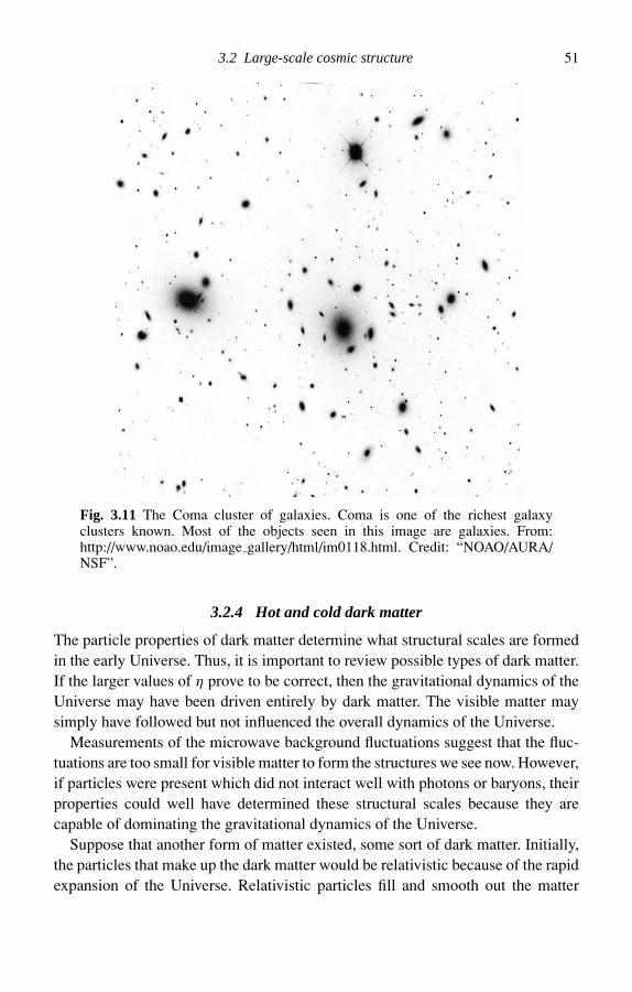
3.2 Large-scale cosmic structure 51
Fig. 3.11 The Coma cluster of galaxies. Coma is one of the richest galaxyclusters known. Most of the objects seen in this image are galaxies. From:http://www.noao.edu/image gallery/html/im0118.html. Credit: “NOAO/AURA/NSF”.
3.2.4 Hot and cold dark matter
The particle properties of dark matter determine what structural scales are formedin the early Universe. Thus, it is important to review possible types of dark matter.If the larger values of η prove to be correct, then the gravitational dynamics of theUniverse may have been driven entirely by dark matter. The visible matter maysimply have followed but not influenced the overall dynamics of the Universe.
Measurements of the microwave background fluctuations suggest that the fluc-tuations are too small for visible matter to form the structures we see now. However,if particles were present which did not interact well with photons or baryons, theirproperties could well have determined these structural scales because they arecapable of dominating the gravitational dynamics of the Universe.
Suppose that another form of matter existed, some sort of dark matter. Initially,the particles that make up the dark matter would be relativistic because of the rapidexpansion of the Universe. Relativistic particles fill and smooth out the matter

52 Cosmic expansion and structure
distribution in a horizon sphere of size 2ct∗
R∗ ≈ ct∗ (71)
so that at epoch t∗, the largest mass structure is given by
M = 4
3R3
∗( ε
c2
)(72)
where ε is the energy density of the sphere.As the Universe cools, the particles become sub-relativistic when the temperature
drops to
T∗ = m∗c2
k(73)
where m∗ is the mass of the particle. The epoch corresponding to a temperature T∗is given by
t∗ ∝ T −2∗ (74)
and the energy density by
ε∗ ∝ (kT∗)4. (75)
Combining (72), (73), (74) and (75)
⇒ M ∝ m−2∗ .
The exact solution is given by
M ≈ 1015
(30 eV
m∗
)2
M (76)
where m∗ is in electronvolt units. Thus, the mass of the dark matter particle has adirect bearing on how small a fluctuation can exist in the matter-dominated Universe.
For a particle with mc2 ≈ 30 eV, → M ≈ 1015 M. This is one prediction ofHot Dark Matter.
On the other hand, for a particle with mc2 ≈ 1 MeV, → M ≈ 106 M. This isthe prediction of Cold Dark Matter.
3.2.5 The Jeans’ mass and gravitational stability
Primordial density fluctuations are constrained to having a minimum mass becausethe conditions at decoupling are such that the thermal pressure of matter can balancegravitational collapse (Chapter 5). We now calculate the minimum mass based onwhat we know about primordial fluctuations.

3.2 Large-scale cosmic structure 53
In terms of the total energy we have the following three cases that define dynam-ical stability
2Ek + EG = 0 static equilibrium
Ek < −1
2EG collapse
Ek > −1
2EG expansion.
In the case of galaxy clusters the kinetic energy refers to the motion of individualgalaxies. In the case of a clump of gas, it refers to the motion of the individual gasparticles, the atoms. Thus, for a parcel of gas, assumed to be ideal, we can rewritethe condition for collapse as
Ek = 3
2NkT < −1
2EG
⇒ 3NkT <G M2
〈R〉 Jeans’ Condition. (77)
From the Jeans’ condition we see that there is a minimum mass below which thethermal pressure prevents gravitational collapse.
Mmin = MJ =(
3NkT 〈R〉G
)1/2
.
The number of atoms corresponding to the Jeans’ mass is given by
N = MJ
m pµ(78)
where µ is the mean molecular weight of the gas and m p is the mass of the proton.In terms of the mass density, ρ,
MJ = 4
3ρ〈R〉3. (79)
Combining (77), (78) and (79)
MJ = ρ−1/2T 3/2
(5k
Gµm p
)3/2 (3
4
)1/2
.
As expected, high density favors collapse while high temperature favors largerJeans’ mass. In units favored by astronomers this condition becomes
MJ ≈ 45 MT 3/2k n−1/2
cm−3 . (80)

54 Cosmic expansion and structure
At the era of decoupling, Tk ≈ 3000 and n ≈ 6 × 10³. Inserting into equation(80) yields
MJ (tD) ≈ 105 M.
Thus, the smallest possible mass capable of collapse at the time of decouplingwas 105 M (assuming that those scales exist). That is about the mass of a globularcluster today. Nothing smaller could have formed. By contrast, in the interstellarmedium of our Galaxy where T ≈ 50 K and n ≈ 103 the Jeans’ mass is ≈ 500 M.Now, far smaller parcels of gas can collapse. That is why molecular clouds cancollapse and form individual stars. The Jeans’ mass at recombination is an importantconstraint on models attempting to explain how galaxies formed.
3.2.6 Possible models of structure formation
Any theory that attempts to explain large-scale structure must account for:
(a) The presence of clusters, superclusters and voids.(b) The r−1.8 scale-invariant correlation law.(c) The minimum mass at decoupling.(d) The role of dark matter.
There are two major competing models that attempt to explain the formationof the large scale structure that we now see. One model begins with the largeststructures forming first and the smallest structures forming last. The other proposesthat smallest structures form first which then coalesce to form larger structures. Thetwo models are summarized below.
(A) The top-down scenario
Largest structures form first because the expanding hot dark matter smoothes out allsmaller scales.
Other, smaller structures result from subsequent fragmentation of the largest structures. Galaxies form last in this fragmentation process. The fragmentation follows the r−1.8 law. Hot dark matter is needed to form the large structures from the primordial fluctuations.
(B) The bottom-up scenario
Objects with M ≈ 105−6 M form first because that is the minimum mass allowedaccording to the Jeans’ criterion.
Larger structures result from gravitational interactions of the smaller structures. Galaxies form before larger-scale structure. The r−1.8 structure law is achievable. Structure exists on small scales because of the dominance of cold dark matter (CDM).

3.4 Further reading 55
In recent years, the realization that the cosmological constant may play a role in theexpansion of the Universe, has led to the development of models that incorporatenonzero values of Λ. The favored models now are those that utilize CDM andnonzero Λ. A more detailed discussion of the early Universe (the time beforedecoupling of matter and radiation) is presented in Chapter 5.
3.3 References
Narlikar, J. V. (1993) Introduction to Cosmology, Cambridge University Press,Cambridge, UK.
Perlmutter, S. et al. (1999) Measurements of Omega and Lambda from 42 High-RedshiftSupernovae, Astrophysical Journal, 517, pp. 565–86.
3.4 Further reading
Coles, P. and Ellis, G. F. R. (1997) Is the Universe Open or Closed?: The Density ofMatter in the Universe, Cambridge University Press, New York, NY, USA.
Combes, F., Mamon, G. A., Charmandaris, V. (Eds) (2000) Dynamics of Galaxies: Fromthe Early Universe to the Present, Astronomical Society of the Pacific, San Francisco,CA, USA.
Dekel, A. and Ostriker, J. (Eds) (1999) Formation of Structure in the Universe, CambridgeUniversity Press, Cambridge, UK.
Fairall, A. P. (Ed). (1998) Large-Scale Structures in the Universe, John Wiley and Sons,New York, NY, USA.
Harrison, E. (2000) Cosmology: The Science of the Universe, Cambridge UniversityPress, Cambridge, UK.
Harwitt, M. (1991) Astrophysical Concepts, Springer-Verlag, New York, NY, USA.Liddle, A. R. and Lyth, D. H. (2000) Cosmological Inflation and Large Scale Structure,
Cambridge University Press, Cambridge, UK.Peacock, J. A. (1999) Cosmological Physics, Cambridge University Press, Cambridge,
UK.Peebles, P. J. E. (1993) Physical Cosmology, Princeton University Press, Princeton, NJ,
USA.Rees, M. (2000) New Perspectives in Astrophysical Cosmology, Cambridge University
Press, Cambridge, UK.


Part II
Statistical mechanics
There are about 1080 particles in the Universe. Most of them are concentrated instars though some can be found in interstellar and intergalactic space. At the centersof stars, particle densities are sufficiently high to allow nuclear reactions to takeplace. The energy liberated by these reactions heats the gas that makes up the starto the point where the gas pressure balances the gravitational pressure leading tohydrostatic equilibrium and long-term stability. Stars like the Sun are stable forabout 1010 years, a large fraction of the age of the Universe.
The radiation produced by the nuclear reactions achieves a near equilibrium withthe gas particles in the stellar interior, leading to local (but not global) thermody-namic equilibrium. The presence of local thermodynamic equilibrium (LTE) meansthat radiation inside the star is close to that of a black body at the local tempera-ture. The absence of global equilibrium allows the radiation to leak out through thesurface of the star and into space. Thus, stars are objects which attain hydrostaticequilibrium and radiate as near-black bodies for most of their lives.
The early Universe, just after the Big Bang, was much like the interior of the star.The radiation from that epoch has the characteristics of black-body radiation and wesee it nowadays as the 2.7 K cosmic background radiation. The early Universe alsoexperienced a period of thermonuclear reactions when most of the hydrogen andhelium was produced. The Universe, of course, is not in hydrostatic equilibrium,which has resulted in a variety of dynamical and physical changes as describedlater in this book.
The thermodynamics that drive the evolution of the Universe and its constituents,can be described in terms of the interaction of particles with radiation and withthemselves. The statistical properties of particles and their grouping into “bosons”and “fermions” are key to understanding the statistical physics that underlie thethermodynamics of the Universe. To that end, this part of the book is dedicatedto reviewing and using concepts from statistical mechanics to gain a better un-derstanding of astrophysical objects. The part begins with a discussion of particle
57
58 Statistical mechanics
distributions which are subsequently used to describe the interior structure of stars,the thermodynamics of the early Universe and the properties of radiation. Specifictopics include basic thermodynamics, Planck’s Law and black-body radiation, the3 K background radiation and the Big Bang, nucleosynthesis and reaction equilibriain the early Universe, stellar structure, properties of white dwarfs and the propertiesof neutron stars and pulsars.

Chapter 4
Overview of statistical mechanics
4.1 Thermodynamics
Many astrophysical bodies are close to thermodynamic equilibrium. A proper un-derstanding of them requires that we understand the basic thermodynamic processesthat control their properties. I begin with a review of classical and quantum me-chanical statistical mechanics. The immediate goal of the review is to derive anddiscuss the equations that define Bose–Einstein and Fermi–Dirac statistics, the twodistributions that govern the behavior of the particles that make up astrophysicalbodies.
Let us consider a simple thermodynamic system consisting of two subsystemsin physical contact as shown in Fig. 4.1. Each subsystem is characterized by thethermodynamic variables of energy (E), volume (V ) and entropy (S). The systemis constrained by the conservation of total energy and volume. Once allowed tointeract the total system comes into equilibrium when the total entropy no longerchanges.
From the first law of thermodynamics
dE = T dS − P dV (81)
where T and P are the temperature and pressure, respectively. Solving for dS, andsetting it to zero,
dS = dE + P dV
T= dE1
T1+ P1 dV1
T1+ dE2
T2+ P2
T2dV2
=(
1
T1− 1
T2
)dE1 +
(P1
T1− P2
T2
)dV1 = 0. (82)
We see that the entropy will stop changing when T1 = T2 and P1 = P2. In otherwords, when the total system has achieved mechanical and thermal equilibrium theentropy is maximized and stops changing.
59

60 Statistical mechanics
S1
V1
E1 E2
V2
S2
S = S1 + S2 dS = 0
V = V1 + V2 = constant
E = E1 + E2 = constant
Fig. 4.1 A system consisting of two subsystems. Energy is conserved in the systembut not within the subsystems. The two subsystems interact until the entropy stopschanging and equilibrium is achieved.
There are other means by which energy can be exchanged. Chemical reactions,for example, can be added to (81), so that
dE = T dS − P dV + µ dN (83)
where we have introduced the chemical potential, µ, and the number of particles,N . The result represented by (82) can now be generalized to
dS =(
1
T1− 1
T2
)dE1 +
(P1
T1− P2
T2
)dV1 −
(µ1
T1− µ2
T2
)dN1 (84)
Thus, if µ1 > µ2, T1 = T2 and P1 = P2 ⇒ dN1 < 0 for dS > 0. With this manyvariables there are many interrelationships that define how changes in one variableaffect other properties. A summary of commonly used thermodynamic terms is asfollows:
Energy E = T S − PV + µN → dE = T dS − P dV + µ dN (85)
Enthalpy H = E + PV → dH = T dS + µ dN + V dP (86)
Helmholtz free energy F = E − T S → dF = −S dT − P dV + µ dN (87)
Gibbs free energy G = E − T S + PV → dG = −S dT + V dP + µ dN (88)
Grand potential Ω = E − T S − µN → dΩ = −S dT − P dV − N dµ. (89)
Combining these equations yields the further relations
G = µN Ω = −PV .

4.2 Classical statistical mechanics 61
GB
GA
B p
has
e sp
ace
A phase space
Fig. 4.2 The phase space AB. The individual phase spaces of A and B form acombined phase space AB.
4.2 Classical statistical mechanics
Some basic concepts are now discussed. These are the grand canonical ensemble,the partition function and the grand potential.
A grand canonical ensemble is an ensemble of a large number of systems. Eachsystem consists of a subsystem A surrounded by a much larger subsystem B, whichtogether form a closed system containing a large number of particles. Within thesubsystem A, the quantities N and E are not necessarily conserved. Consider theschematic of the combined phase space of the system AB, as shown in Fig. 4.2. Anelemental volume in the phase space of A and B is given by
dΓA = d3qA d3 pA
dΓB = d3qB d3 pB .
Now, let DA+B be the density of system points in Γ space. The probability of aspecific macrostate is given by
DA+B = DA DB → ln DA+B = ln DA + ln DB
⇒ DA+B = constant. Density DA+B is a conserved quantity! In other words, thesystem will eventually reach equilibrium, that is ln DA+B approaches a constant intime.
From our previous discussion regarding conservation laws and the fact that thisis a constant sum that looks like a conservation law, we should be able to expressln D as a linear combination of energy and particle number (since those are the

62 Statistical mechanics
quantities that must be conserved in the system AB) such that
ln DA = αA + βµNA − βE A.
Thus, for subsystem A
D = constant × eβ(µN−HN )
where HN = HN (q, p) is the Hamiltonian representing the total energy of all NA
particles and we have generalized the notation by replacing NA with N . Dimen-sionally, β must also have units of energy. Identifying β as the inverse of the thermalenergy we have
D = constant × e(µN−HN )/kT .
This expression requires normalization which can be achieved through the definition
DN ≡ 1
Qe(µN−HN )/kT . (90)
The normalization condition then becomes∞∑
N=0
∫DN dΓN = 1
Q
∞∑N=0
eµN /kT∫
e−HN (q,p)/kT d3Nq d3N p = 1.
Solving this for Q yields
Q(T, V, µ) ≡∞∑
N=0
∫e(µN−HN (q,p))/kT d3N q d3N p. (91)
The integral has the name canonical partition function while the summed quantityQ(T, V, µ) is called the grand canonical partition function. We can make theconnection with the thermodynamic equations by setting
S = −k∞∑
N=0
∫DN ln DN dΓN . (92)
We can see that this is the correct choice by substituting (90) into (92) so that
S = −k∞∑
N=0
∫DN
[1
kT(µN − HN ) − ln Q
]dΓN
= −µ
T〈N 〉 + 1
T〈HN 〉 + k ln Q (93)
where the angle brackets represent the operation
〈X〉 ≡∞∑
N=0
∫X DN dΓN

4.3 Quantum statistical mechanics 63
known as the grand canonical ensemble average. Rearrangement of (93) gives
T S = −µN + E + kT ln Q. (94)
Comparing with (89) yields the definition of Q
Ω ≡ −kT ln [Q(T, V, µ)] (95)
the grand potential. Thus, the connection with the thermodynamic equations iscomplete.
4.3 Quantum statistical mechanics
The transition to quantum mechanics requires that we recognize the discretenessof energy levels associated with individual particles.
HN =∑
j
N jε j (96)
where∑
j N j = N , the total occupation number. The transformation from classicalto quantum statistical mechanics therefore requires
Q =∞∑
N=0
∫e(µN−HN )/kT dΓN ⇒
∑N j
e∑
j N j (µ−ε j )/kT . (97)
If we use the identity
e∑
j x j = Πj
ex j
(97) becomes
Q(T, V, µ) =∑N j
[Πj
yN j
j
](98)
where
y j ≡ e(µ−ε j )/kT . (99)
If we now use the additional identity
∑N j
[Πj
α j (N j )
]≡ Π
j
∑
N j α j (N j )
we end up with
Q(T, V, µ) = Πj
∑N j
yN j
j . (100)

64 Statistical mechanics
This result places us in a better position to discuss Bose–Einstein and Fermi–Diracstatistics.
4.3.1 Bose–Einstein statistics
Recall that power series can have convergent sums, so that∞∑
N j =0
yN j
j = 1 + y j + y2j + · · · = 1
1 − y j(101)
where y < 1. Combining (100) and (101)
⇒ Q = Πj
1
1 − y j.
Substituting into the definition of the grand potential and using (99) we obtain
Ω = −kT ln Q = kT∑
j
ln[1 − e(µ−ε j )/kT
]. (102)
From (89), N = − (∂Ω/∂µ)T,V so that
N =∑
j
e(µ−ε j )/kT
1 − e(µ−ε j )/kT=
∑j
1
e(ε j −µ)/kT − 1. (103)
Identifying the quantity inside the summation sign as the average occupationnumber, we finally have
〈N j 〉 = 1
e(ε j −µ)/kT − 1. (104)
4.3.2 Fermi–Dirac statistics
The Pauli exclusion principle requires that N j = 0, 1 only. Thus∑j
yN j
j = 1 + y j
so that
Ω = −kT ln Q = −kT∑
j
ln[1 + e(µ−ε j )/kT
]with
N = −(
∂Ω
∂µ
)T,V
≡∑
j
〈N j 〉
⇒ 〈N j 〉 = 1
e(ε j −µ)/kT + 1. (105)

4.4 Photon distribution function 65
dA
dx
n
k
Fig. 4.3 Elemental surface. The beam direction, k, and the normal to the surface,n, are shown.
Ωd
p
dp
Fig. 4.4 Elemental volume. The relationship between the elemental momentumvolume and the elemental solid angle is shown.
We can see that the distribution functions, equations (104) and (105), reflect thedifferent constraints on the occupation number.
4.4 Photon distribution function
Let us define a function that describes the number of photons of spin state (polar-ization) α, at time t , in a phase element centered at x , p. For photons
α = 1, 2 p = hk = hν
ck. (106)
Thus the radiant energy per phase element is
dE =2∑
α=1
hν Fα(x, p, t) d3x d3 p. (107)
For a beam of photons (Figs. 4.3 and 4.4)
dV = d3x = dxdA = k · nc dt dA (108)
d3 p = p2 dΩ dp = h3ν2
c3dΩ dν from (106). (109)
66 Statistical mechanics
Combining (107), (108) and (109)
⇒ dE =2∑1
hνFα(x, p, t)k · n c dt dAh3ν2
c3dΩ dν
= h4ν3
c2
2∑1
Fα(x, p, t)k · n dA dΩ dν dt. (110)
Let us now compare (110) with the definition of specific intensity, Iν(k, x, t),
dE = Iν(k, x, t)k · n dA dΩ dν dt.
We see that
Iν =2∑1
h4ν3
c2Fα(x, p, t). (111)
This places us in a position to define an occupation number for each spin state, thatis an occupation number per phase cell
Nα ≡ h3 Fα (112)
so that (111) can be rewritten as
Iν =2∑1
hν3
c2Nα(x, p, t). (113)
Equation (113) represents a relationship between the intensity of a beam ofphotons and the occupation number which describes the statistical behavior of thephotons with respect to the phase space. Under thermodynamic equilibrium, (111)and (113) are constrained to specific functional forms. We now consider those.
4.5 Thermodynamic equilibrium
Kirchhoff showed that under thermodynamic equilibrium
Iν = Bν(T ) (114)
the spectrum of emitted radiation depends only on the temperature of the emittingbody. Planck showed that the specific functional form of Bν is given by
Bν = 2hν3/c2
ehν/kT − 1. (115)
Proper derivation of (115) from (113) requires knowledge of Bose–Einstein statis-tics given that photons are bosons. Since we defined the latter in the previous

4.5 Thermodynamic equilibrium 67
100 200 300 400 500400
300
200
100
01.0 0.2 0.1 0.07 0.05
Frequency (GHz)
Inte
nsity
(M
Jy/s
r)
Wavelength (cm)
T = 2.725 ± 0.001 K
Fig. 4.5 The 3 K background spectrum. The measurements were made by theFIRAS instrument on COBE. The best curve yields a temperature of 2.725 K. Thisfigure was obtained from http://space.gsfc.nasa.gov/astro/cobe.
subsection let us do that. Using (104) and the knowledge that for photons, µ = 0we have
Nα = 1
ehν/kT − 1. (116)
Substituting (116) into (113) yields (114) and (115). It is useful to examine theseresults in limits of high and low photon energy.
For hν kT
Nα = e−hν/kT
which represents the classical Boltzmann distribution. Photons act like particles.For hν kT
Nα = kT
hν 1
which is in the Rayleigh–Jeans Limit. In a single phase cell, E = hνNα = kT andphotons act like waves.
An example of a black-body spectrum is shown in Fig. 4.5. It is the spectrumexpected from a body in thermodynamic equilibrium at a temperature of 2.7 K.It is also the best fit curve for measurements made of the cosmic background
68 4.6 Further reading
radiation with the FIRAS detector on the COBE satellite (see COBE homepage –http://space.gsfc.nasa.gov/astro/cobe). The curve in Fig. 4.5 represents a perfectblack body to within the experimental errors, which tells us that the cosmic 3 Kradiation was originally emitted under conditions of thermodynamic equilibrium.Since the modern day Universe consists of both matter and radiation, these twocomponents were, at one time, in equilibrium. When was that and what is theimplication of this result on galaxy formation? That is the subject of the nextchapter.
4.6 Further reading
Garrod, C. (1994) Statistical Mechanics and Thermodynamics, Oxford University Press,New York, NY, USA.
Kittel, C. (1980) Thermal Physics, 2nd edn, Freeman, San Francisco, CA, USA.Pauli, W. (2000) Thermodynamics and the Kinetic Theory of Gases, Dover, New York,
NY, USA.Shu, F. H. (1992) The Physics of Astrophysics: Radiation, University Science Books, Mill
Valley, CA, USA.

Chapter 5
The early Universe
5.1 The 3 K background radiation
According to the COBE results, the thermal properties of the cosmic backgroundradiation are characterized by a temperature of
T = 2.725 ± 0.006 K
and temperature fluctuations of
T
T= 6 × 10⁻⁶
which represent the spatial variation of temperature across the sky. These resultshave fundamental importance with respect to our knowledge of the early Universeand the formation of galaxies. Given our earlier discussion of the gravitationaldynamics of the Universe and given what we now know about the background radi-ation, let us evolve the “radiation” Universe back in time to see what we can learn.
5.1.1 History of the background radiation
According to energy conservation and the equations developed in Section 3.1
ET = Ek + EG = 2
5ρH 2 R5 − 162
15ρ2G R5 = constant. (117)
We know that ρ = M/( 43 R3), H = v/R so that (117) can be cast into the form
ET = 0.3Mv2 − 3
5G M2 R−1
⇒ v2 − 2G M
R= ET
M
10
3= E
⇒ dR
dt=
√E + 2G M
R(118)
69

70 The early Universe
⇒ dR√E + (2G M/R)= dt
⇒∫ R
0
dR′√E + (2G M/R′)
=∫ t
0dt ′.
This equation represents the evolution of R(t) for a given energy and mass of theUniverse.
We can consider the three special cases corresponding to flat, open and closedUniverses.
Flat Universe (E = 0)
In this case, the integral is trivial
1√2G M
∫ R
0dR′√R′ = t
⇒ R(t) =(
3
2
)2/3
(2G M)1/3t2/3 =(
9
2G M
)1/3
t2/3. (119)
The radius increases as t2/3.
Open Universe (E > 0)
When the Universe has a positive total energy its long-term evolution is determinedby the excess kinetic energy. In that case, the solution to (118) is more complex.The author has used the software package MAPLE to obtain the solution below.√
R2
E + 2G M R
E2− G M
E3/2ln
[2√E2 R2
2EG M R + 2ER + 2G M] = t. (120)
Closed Universe (E < 0)
When the total energy is negative the gravitational attraction of the matter wins outin the long term and the Universe eventually collapses. The solution, obtained in asimilar way, becomes
⇒ G M
E3/2arcsin
[ ER
G M− 1
]−
√2G M R
E2− R2
E = t. (121)
5.1.2 Evolution of energy density
Recall that the quantity E represents energy density. Let us now consider the energydensity of the photons.
Eγ = nγ hν. (122)

5.2 Galaxy formation 71
But the number density, Nγ has the behavior nγ ∝ R−3 and the frequency of aphoton goes as ν ∝ 1/λ ∝ 1/R as a result of being redshifted by the expansion.Thus, according to (122)
Eγ ∝ R−4.
But, Eγ ∝ T 4 ⇒ T ∝ 1/R. Combining all of this, we have
⇒ T
T0= R0
R. (123)
Combining (123) and (119)
⇒ T
T0=
(t0t
)2/3
(124)
for a flat Universe. This is a good scaling law even for E = 0 so long as E is closeto 0. The scaling law is valid only for t > tD after the decoupling time. For timesbefore decoupling the radiation pressure of the photons dominated the dynamics ofthe Universe.
It is now possible to evolve the Universe back in time using this scaling law.As starting points we will use contemporary values of T0 = 2.7 K and t0 = 1.4 ×10¹⁰ years. Let us evolve the Universe back in time when T = 3000 K, the era ofdecoupling. The age of the Universe would then have been
tD =(
T0
T
)3/2
t0 = 4 × 10⁵ years.
Thus, for times t ≤ 4 × 10⁵ years, radiation and matter would have been tightlycoupled because the photons were energetic enough to keep matter ionized. Duringthis time the Universe was radiation dominated in the sense that radiation energydensity was greater than the energy density of matter. Any clustering of matterduring this epoch would have to be accompanied by a clustering of radiation energydensity (i.e. a temperature enhancement).
5.2 Galaxy formation
In the hot-dark-matter (HDM) top-down scenario, the modern day structure requiresthat
ρ
ρ> 10−4
at time of decoupling, where ρ is the matter density. Otherwise Hubble expansionand gravitation alone could not produce the modern day large scale structure. Just

72 The early Universe
before decoupling, matter and radiation were coupled so that the density enhance-ments must also show up as temperature enhancements
ρ
ρ= (T 4)
T 4= 4T
T(125)
so that the HDM model would predict
ρ
ρ> 10−4 ⇒ T
T> 2.5 × 10⁻⁵.
Now, according to COBE, T/T ≈ 6 × 10⁻⁶ K, which argues against a purelyHDM model.
Now, some cold-dark-matter (CDM) models predict
T
T> 4 × 10⁻⁶ K
and they cannot be ruled out by the COBE observations. On the other hand, CDMhas difficulty accounting for the largest structures in the Universe. For these reasonshybrid models, combining HDM and CDM, were introduced. However, the possi-bility of a nonzero cosmological constant makes the hybrid models less relevant.In fact, CDM, in conjunction with a nonzero Λ can satisfactorily account for thelarge scale structure, as discussed in Chapter 3.
5.3 Local cosmology and nucleosynthesis
5.3.1 Overview
As noted in the previous section, the energy density of the Universe was much higherin the past. Before decoupling, matter and radiation were in close equilibrium andthere were times during the early evolution of the Universe when the conditions weresimilar to those found in the interiors of stars such as the Sun. In other words, thedensity, temperature and pressure were high enough for thermonuclear reactionsto take place and for nucleosynthesis to occur. Consequently the following areexamples of cosmological questions.
Why is 10−5 of the seawater “heavy”? In other words why is the ratio [D/H] ≈ 10−5? Why is 25% of the Sun’s mass in the form of 4He?
The reason the above are cosmological questions is that there is no known process inthe current Universe to account for the above ratios. There is simply too much 2D and4He (and 7Li) around. Yet we know that these elements can be produced in simplenuclear reactions whose physics are understood. With scaling laws in hand, we knowthat if we evolve the Universe back in time the conditions for nucleosynthesis existed

5.3 Local cosmology and nucleosynthesis 73
for t ≤ 1 ms. Having estimated these conditions and knowing how nuclear reactionsoperate (they are governed by readily understood laws of physics) it is possible forus to estimate how much 2D and 4He (and 7Li) could have been produced duringthe Big Bang. Such calculations indicate that the currently observed abundancesof these elements can be entirely explained as resulting from the Big Bang. Thesuccess of these calculations gives great weight to the Big Bang hypothesis and givesresearchers the confidence to examine the physics of the Universe back to t ≈ 10−35
seconds and to contemplate the birth of the Universe and its basic elements.Despite the fact that BBN can account for the current abundances of 2D and
4He (and 7Li) we should still ask the question – can these elements be producedin a more conventional manner? Could 2D and 4He (and 7Li) be products of stellarnucleosynthesis (such as takes place in the core of the Sun)?
5.3.2 Primordial helium
All main-sequence stars produce 4He in their cores. These elements are dispersedinto the interstellar medium through stellar winds, ejection of planetary nebulasand supernova explosions. So why cannot these processes account for the currentabundance of 4He in the Universe? Let us answer that question quantitatively byexamining how much energy is needed to make a 4He atom from 4 nucleons. Westart off with the definition of an atomic mass unit (amu),
1 amu = 931.478 MeV/c2.
Table 5.1 lists the mass defects of some simple elements.When 4p → 4He + Q, the energy released is Q = 26.7 MeV, of which about
1.6 MeV is in the form of neutrinos. Thus, the formation of the 4He atom is accom-panied by the release of > 25 MeV ≈ 4 × 10⁻⁵ ergs.
If we now take all the nucleons in the Universe
〈nnucleons〉 ≥ 10−7 cm−3
Table 5.1. Mass defects
Element (M − A) × amu c2 (M − A)/A
n 8.07 MeV 8.07 MeVp 7.29 MeV 7.29 MeV2H = D 13.14 MeV 6.57 MeV3He 14.93 MeV 4.98 MeV4He = α 2.42 MeV 0.61 MeV12C 0 0

74 The early Universe
we can make
→ ⟨n(4He)
⟩ ≈ 0.25nucleon
4≥ 6 × 10⁻⁹ cm−3.
helium nuclei. The energy associated with making this many helium nuclei is thengiven by
〈Eα〉 ≈ 4 × 10−5 erg × 6 × 10−9 cm−3 = 2 × 10⁻¹³ erg cm−3.
Now, most of the luminosity of the Universe arises ultimately from theproduction of 4He. The mean luminosity density of the Universe is known to be≈ 2 × 10⁻³² erg s−1 cm−3. Thus, in the 1010 years = 3 × 10¹⁷ seconds, duringwhich stars have existed, the amount of energy arising from 4He production is
〈EL〉 ≈ 6 × 10⁻¹⁵ erg cm−3.
Thus, the ratio of energy densities resulting from actual helium production to thatneeded to account for the observed amount is
〈EL〉〈Eα〉 ≈ 0.03.
Thus, if all the luminosity of the Universe were used to make 4He over the entireage of the Universe it could change the present amount by only a few percent. Thusthe 4He must be primordial. What about D?
The number density of D is
〈nD〉 = 10−5〈nN 〉 ≈ 10−12 cm−3.
The element D is most easily made in the reaction
n + p → D + Q; Q = 2.2 MeV
p + p → Q + Q; Q = 3 MeV
so that the energy density associated with the formation of D is given by
〈ED〉 ≈ 3 MeV × 10−12 cm−3 ≈ 5 × 10⁻¹⁸ erg cm−3 〈EL〉.There is no problem accounting for D given the current nuclear reactions going on inthe Universe. However, D is very hard to preserve once it is made. The environmentsin which it is currently made (stellar interiors) are conducive to the destruction ofD. This can best be illustrated in the context of nuclear reaction rates which wediscuss now.

5.4 Reaction rates 75
5.4 Reaction rates
5.4.1 Introduction
Consider the generic reaction
a + X → Y + b + Q
where X is stationary and there is a flux of incident particles a having a density na
and velocity v. Then
flux = nav
cross-section = σ (v) ≡ reactions/time (per X particle)
flux of a (particles area−1 time−1).
So that the number of reactions volume−1 second−1 are
raX = nanX 〈σv〉where v is the relative velocity and
〈σv〉 ≡∫ ∞
0σ (v)φ(v)v dv
where φ(v) is the normalized relative velocity distribution such that∫φ(v) dv = 1.
For a non-degenerate gas (defined in Section 5.5)
φ(v) dv ∝ e−E/kT︸ ︷︷ ︸Boltzmann factor
v2 dv︸ ︷︷ ︸phase space factor
φ(v) =( µ
2kT
)3/2e[−(µv2)/(2kT )] 4v2
µ = mam X
ma + m X= reduced mass.
The reaction cross-section is governed by nuclear attraction at small distances andCoulomb repulsion at larger distances. The nuclear attraction represents a bindingenergy which is typically around 8 MeV/nucleon (see Table 5.1). Thus, Qreaction isalways ≈ MeV.
The range of the attractive nuclear force is given by
R ≈ A1/3 × 10−13 cm = A1/3 fm.

76 The early Universe
R
ro
E =kTVc
Q
E
r
Fig. 5.1 The Coulomb barrier. A particle with E = kT traveling leftward fromr = ∞ will see a Coulomb barrier of amplitude Vc and scale r0. The nuclearpotential well, depth Q and scale R is also shown.
On the other hand, Coulomb repulsion is described by
V = qaqX
r= Za Z X × e2
R
= 1.44Za Z X
R(fm)MeV.
The excess energy is the result of having to overcome the Coulomb barrier.Typically, the kinetic energies of the particles undergoing nuclear reactions have
Ek ≈ kT ≈ 1 keV (Sun)
Ek ≈ kT ≈ 10 keV (BBN).
We see that Ek Vcoulomb so that classically nuclear reactions are impossible. Thedistance r0 at which the Coulomb potential equals the kinetic energy of the incidentparticle (Fig. 5.1) is then r0 ≈ 103 R. Classically the incident particle turns backvery far from the region where nuclear reactions can take place. The reason thatnuclear reactions take place at all is because of quantum mechanical tunneling. Wenow review the concept of tunneling by discussing the QM 1-D potential barrier.
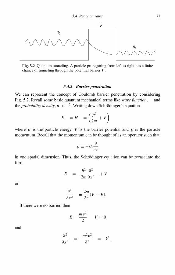
5.4 Reaction rates 77
n0
V
n1
Fig. 5.2 Quantum tunneling. A particle propagating from left to right has a finitechance of tunneling through the potential barrier V .
5.4.2 Barrier penetration
We can represent the concept of Coulomb barrier penetration by consideringFig. 5.2. Recall some basic quantum mechanical terms like wave function, Ψ andthe probability density, n ∝ Ψ 2. Writing down Schrodinger’s equation
EΨ = HΨ =(
p2
2m+ V
)Ψ
where E is the particle energy, V is the barrier potential and p is the particlemomentum. Recall that the momentum can be thought of as an operator such that
p ≡ −i h∂
∂x
in one spatial dimension. Thus, the Schrodinger equation can be recast into theform
EΨ = − h2
2m
∂2
∂x2Ψ + V Ψ
or
∂2
∂x2Ψ = 2m
h2(V − E)Ψ.
If there were no barrier, then
E = mv2
2V = 0
and
∂2
∂x2Ψ = −m2v2
h2Ψ = −k2Ψ.

78 The early Universe
This is just the equation for a traveling wave, meaning that the particle travels alongunimpeded. The wave function then becomes
Ψ = Ψ0 e±ikx
and particle motion is possible in either direction. The probability density is thengiven by
|Ψ |2 = Ψ Ψ ∗ = |Ψ0|2 = constant
as expected.With the barrier in place, V > 0 and we have
∂2
∂x2Ψ = 2m
h2(V − E)Ψ ≡ λ2Ψ
for which the solution is
Ψ = Ψ0 e−λx + Ψ1 e+λx︸ ︷︷ ︸→0
since we require that the probability density be bounded over an infinite volume.Thus, the probability density is given by
|Ψ |2 = |Ψ0|2 e−2λx .
The penetration is characterized by the parameter
P = |Ψ (xb)|2|Ψ0|2 = e−2λxb .
where, xb = 1/(2λ) is the scale length for the penetration and
λ =[
2m
h2(V − E)
]1/2
.
The larger the V and the smaller the energy of the particle the harder it is forbarrier penetration to work. However, the exponential dependence of the effectensures that the probability for penetration is always finite.
Gamow Peak
In real life V = V (x) thereby complicating this simple picture. These results wouldhave to be generalized so that
ln P ≈ 2∫
λ(x) dx .

5.4 Reaction rates 79
Consequently, the relevant integral is
ln P = 2∫ R
r0
λ(r ) dr
= 2∫ R
r0
[2m
h2
(Za Z X e2
r− mv2
0
2
)]1/2
dr.
The classical turning point is defined by the condition
Za Z X e2
r0≡ mv2
0
2.
Thus
ln P = 2
[(2m
h2
) (mv2
0
2
)]1/2 ∫ R
r0
(r0
r− 1
)1/2dr
= 2
[(2m
h2
) (mv2
0
2
)]1/2
r0
∫ R/r0
1
(1
x− 1
)1/2
dx︸ ︷︷ ︸convergent for x→0
where x = r/r0. Setting the integral to a finite value I , we have
ln P = 2
[(2m
h2
) (mv2
0
2
)]1/22Za Z X e2
mv20
I = 4I Za Z X e2
hv0.
The exact solution, generalized for any v, is
P = e−(2Za Z X e2)/(hv).
The convention for defining the cross-section in terms of the penetration param-eter is given by the equation
σ (E) = S(E)
Ee−(2Za Z X e2)/(hv).
The function S(E) depends on the nuclear physics and is weakly dependent on theenergy. Armed with this definition of σ let us turn our attention back to reactionrates
〈σv〉 =∫ ∞
0σφv dv =
∫σφ
dE
µ
where
σ (E) = S(E)
Ee−b/
√E
φ =( µ
2kT
)3/2e−E/kT
(8
µ
)E

80 The early Universe
e−E/kT
e−b/E 1/2
S (E )
<σv>
E
Fig. 5.3 Components of the reaction rate function. The shapes of the three func-tions that make up the expression for 〈σv〉 are shown.
b ≡ 2Za Z X e2
h
(µ
2
)1/2
〈σv〉 =(
8
µ
)1/2 1
(kT )3/2
∫ ∞
0S(E) e[−(E/kT )−(b/
√E)] dE .
Figure 5.3 illustrates the dependence of 〈σv〉 on energy. The exponential in theintegral is sharply peaked at some energy E0. Let us find out what E0 is. We beginby searching for a local extremum in the argument of the exponential
d
dE
[E
kT+ b√
E
]= 0 at E0
1
kT− b
2E3/20
= 0
⇒ E0 =(
bkT
2
)2/3
E0 = 1.2(Z2
a Z2X AredT 2
6
)1/3keV.
This represents the optimal energy for nuclear reactions. The sharp drop off inenergy on either side of E0 gives the cross-section a peaked geometry with respectto energy. The region centered on E0 is known as the Gamow Peak.
5.4 Reaction rates 81
5.4.3 Estimating reaction rates
All that remains now is to estimate the integral in order to obtain a numericalexpression for the reaction rate. Integrals of the form
I =∫ B
AS(E) e− f (E) dE
where f (E) is peaked at E0 can be estimated by the method of steepest descent.Part of the method involves an expansion of f (E) about E0 in a Taylor series.
f (E) ≈ f (E0) + ∂ f
∂ E(E − E0) +
(∂2 f
∂ E2
)E0
(E − E0)2
2+ · · ·
≈ f (E0) +(
∂2 f
∂ E2
)E0
(E − E0)2
2
= f (E0) +(
E − E0
σ
)2
where
σ 2 = 2
(∂2 f/∂ E2)E0
I ≈ e− f (E0)S(E0)∫ ∞
−∞e−[(E−E0)/σ ]2
dE
= σ√
S(E0)e− f (E0).
In our case
f (E) = E
kT+ b√
E
E0 =(
bkT
2
)2/3
kT
f (E0) = 3E0
σ = 2√3
(E0kT )1/2 E0
⇒ raX = nanX7 × 10−19
Ared Za Z XS0(keV barns)τ 2e−τ s−1 cm−3
where
τ = 42.5
(Z2
a Z2X Ared
T6
)1/3

82 The early Universe
where
T6 = T/106 K Ared =(
1
Aa+ 1
AX
)−1
= Aa AX
Aa + AX
Note the very strong dependence on Za Z X . The factor of 42.5 also gives the reactionrate a strong dependence on T6.
5.4.4 Destruction of D
It turns out that
D + p → 3He +
is the most rapid nuclear reaction. If we examine the deuterium lifetime
1
tD= 1
nD
(∂nD
∂t
)= n p〈σv〉Dp
we see that it is short because Z D Z p = 1 has the lowest possible value and protonsare the most abundant constituent. In any environment where D can be made it willbe destroyed. In the Sun
[D/H] ≈ 10−18
reflecting the fact that D is easily destroyed. The destruction of D is what makes itdifficult to preserve. Therefore, the observed cosmic abundance of D can only beexplained if it is primordial. How much D is produced in BBN is critically dependenton the conditions that existed in the early Universe. Explaining its current abundancetells us much about the nature of the early Universe.
5.4.5 Formation of D
When T < 109 K the following reaction forms deuterium
n + p → D + .
However, the D that is formed then participates in a subsequent reaction
D + D →4 He + .
Whereas, the former reaction produces D, the latter one destroys it. The relativerates of the two reactions determine the equilibrium abundance of the deuterium.Generally, the second reaction is the faster of the two and it therefore determinesthe equilibrium value of D.
Using the preceding arguments, the timescale for the DD reaction is
tDD ∝ ρ−1b .

5.5 Particle equilibria 83
where ρb is the baryon mass density. The greater the mass density of the Universe,for example, the faster the DD reaction proceeds and the lower the equilibriumvalue of D. The lower the mass density the greater the D abundance. It is for thisreason that the D abundance is a sensitive tracer of the conditions (density) in theearly Universe.
5.4.6 Formation of 4He
Before Big Bang nucleosynthesis began, the early Universe had plenty of freeneutrons (see next section) and protons. The interaction of n and p leads to theproduction of 4He, as we have noted. If the abundance of n is significantly lowerthan the abundance of p essentially all the n go into making 4He. Thus, the abundanceof 4He is given by
4He ≈ n/2
(n + p)/4= 2n
n + p.
The contemporary ratio of neutrons to protons is about 0.12. Inserting that valueinto the previous equation yields 4He ≈ 2/9, which is the approximate abundanceof 4He in the Universe today.
5.5 Particle equilibria in the early Universe
5.5.1 Overview
The formation of elements in the early Universe can best be understood by con-sidering the environments in which current fundamental particles were in equilib-rium. These particles include well-known baryons such as neutrons and protons,leptons such as electrons, mu neutrinos, electron neutrinos, tau neutrinos and an-tineutrinos, as well as photons. All the particles are, of course, fermions while thephotons are bosons. For the particles to be in equilibrium with each other theirkinetic energies must be comparable to their rest mass energies. Table 5.2 lists therest mass energies of some particles. For temperatures above about 1012 K all ofthe particles are in equilibrium with each other.
Using the temperature scaling law appropriate for cosmic expansion beforedecoupling
t = td ×(
Td
T12
)2
is the time after the Big Bang when the temperature was 1012 K. Using the numbersfrom Section 5.1.5, we obtain t12 = 10−4 seconds. Thus, it appears that 10−4 secondsafter the Big Bang there was an equilibrium between n, p, e+−, , νe, νe, νµ, νµ,
ντ , ντ .

84 The early Universe
Table 5.2. Particle equilibrium temperatures
Particle species A Rest mass energy Teq
Electron/positron 511 keV 6 × 10⁹ KMuon/antimuon 107 MeV 1.2 × 10¹² K and e neutrinos/antineutrinos 0 0Proton/neutron 940 MeV 1013 K∗Pions 140 MeV 1.6 × 10¹² K
∗ Tn − Tp = 1.5 × 10¹⁰ K
N
ε
T = 0
T > 0
1
0µ
Fig. 5.4 Fermion occupancies at T = 0 and T > 0. At T = 0 all states up toµ are filled. At finite temperatures the sharp boundary at µ is softened and thedistribution assumes a more classical form.
The statistical distribution of the fermions is described by (105). Let us examinethe behavior of the occupation number in the limits of strongly negative and stronglypositive chemical potentials because this behavior will illustrate how fermions inthe Universe behave.
For µ −kT equation (105) reduces to
N ≈ e(µ−ε)/kT = e−|µ/kT | e−ε/kT = α e−ε/kT
where α 1. The behavior is exponential, as you would expect.For µ kT we have N ≈ 1 if ε µ and N 1 if ε µ. The corresponding
distribution function is shown in Fig. 5.4 (T = 0).The intermediate case, µ ≈ kT , is an interpolation between the two extreme cases
and is shown in Fig. 5.4 (T > 0). The number density follows from the occupation

5.5 Particle equilibria 85
number according to
n =∑
α
∫d3p
h3Nα(ε). (126)
In the low-density, non-degenerate limit µ kT we have the Maxwell–Boltzmannlimit
n =∑
α
∫d3p
h3eµ/kT e−ε/kT (127)
where
ε = εkinetic︸ ︷︷ ︸εk=p2/(2m)
+ εinternal︸ ︷︷ ︸εα
0︸︷︷︸lowest level
+ εαi︸︷︷︸
excitations
n =∑
α
∫ ∞
0
4p2 dp
h3(eµ/kT ) e−εk/kT e−ε0/kT e−εα
i /kT
= 4 eµ/kT
h3
(∫p2 dp e−εk/kT
)︸ ︷︷ ︸∫
p(p dp) e−εk /kT
(∑α
eεαi /kT
)︸ ︷︷ ︸
g≡internal partition function
e−ε0/kT . (128)
For non-relativistic particles
p = (2mεk)1/2 p dp = m dεk
so that ∫p2 dp e−εk/kT = 1
2(2mkT )3/2
∫ ∞
0
√x e−x dx︸ ︷︷ ︸√/2
so that (128) becomes
n = eµ/kT
(2mkT
h2
)3/2
g e−ε0/kT .
Solving for µ/kT
µ
kT= ln
[(h2
2mkT
)3/2n
g
]+ ε0
kT. (129)
For the Maxwell–Boltzmann limit to hold we require
ln
[(h2
2mkT
)3/2n
g
] −1

86 The early Universe
which is the mathematical way of saying that phase space is not important. Forelectrons without internal excitations g = 2, and the previous expression can bere-expressed as
ne 2
(2mekT
h2
)3/2
= 4.8 × 10¹⁵T 3/2 cm−3
or
ρ ≈ m pne 10−8T 3/2 g cm−3.
We can apply this criterion to a number of astrophysical environments to seewhether the Maxwell–Boltzmann limit is justified. For the Sun, T ≈ 107 K →ρ 300 g cm−3 for complete non-degeneracy. The maximum density of the Sunis ≈ 100 g cm−3 so the criterion is largely satisfied. This is the case for most normalstars. The criterion is not satisfied in the case of white dwarfs which have degen-erate cores. For the Universe as a whole when the electrons were non-relativistic(T < 109 K)
ne ≈ 10−5
(T
2.7
)3
⇒ ne
T 3/2= 10−5 T 3/2
(2.7)3=
(T
109 K
)3/2
2 × 107 cm−3 1015.
The more massive particles have even lower chemical potentials. For nucleons
n 4.8 × 10¹⁵T 3/2
(m p
me
)3/2
≈ 3.7 × 10²⁰T 3/2 cm−3
ρ 6.1 × 10⁻⁴T 3/2 g cm−3 = 6.1 × 10⁸
(T
108 K
)3/2
. (130)
This criterion is satisfied everywhere except in neutron stars. Thus neutron stars andwhite dwarfs are fully degenerate while some stars and Jovian planets are partiallydegenerate. As far as the Universe is concerned it can be considered non-degeneratewhich makes life a lot easier for describing particle reactions in the early Universe.Let us do that now.
5.5.2 Chemical equilibrium
Consider particle species, A, B, C, D. The reaction,
A + B · · · C + D · · ·

5.5 Particle equilibria 87
has the chemical potential relating as:
µA + µB · · · µC + µD · · ·where µi is the chemical potential of species i and represents the energy changefrom adding one particle of type i .
5.5.3 The early Universe
Let us now consider the chemical equilibrium at T = 1010 K. From the previoustable we know that electrons and positrons are in equilibrium. Since the two particlesinteract via the pair production process we know that the following reaction willoccur under equilibrium conditions
+ e+ + e−.
For photons which can be emitted and absorbed in unrestricted quantities, thechemical potential µγ = 0. Therefore
µe+ = −µe− .
We know from observations of the modern day Universe that
n p nγ ≈ ne+ + ne− .
This means that the number density of electrons and positrons is very low relative totheir number before they produced all the photons. Thus, their chemical potential,according to (129), must be relatively low. Thus, to a good approximation, µe+ ≈µe− ≈ 0. A similar statement can be made for the protons, neutrons and neutrinos.
5.5.4 The neutron–proton ratio
The current ratio of neutrons to protons in the Universe can be estimated by ex-amining the nuclei of the elements. To a good approximation this ratio is given bycomparing the abundances of H and He. Thus[
n
p
]≈ 1
2
[He
H
]≈ 12%.
When the temperature of the Universe was 1010 K the neutrons and protons werein equilibrium with the electrons and neutrinos according to these reactions
n + e+ p + νe
n + νe p + e−
n → p + e− + νe (one way).

88 The early Universe
The above is characterized by the chemical balance
µn + µνe = µp + µe−
⇒ µn = µp. (131)
Given the previous discussion these chemical potentials are also close to 0.However, let us use (131) to establish an important relationship between protonsand neutrons. Combining (129) and (131) we have
ln
[(h2
2mnkT
)3/2nn
gn
]+ ε0,n
kT= ln
[(h2
2m pkT
)3/2n p
gp
]+ ε0,p
kT.
Now, gn ≈ gp ≈ 2. Also, mn ≈ m p is a good approximation for the slowly varyinglogarithmic term. Thus, this simplifies to
ln nn + ε0,n
kT= ln n p + ε0,p
kT
⇒ ln
(nn
n p
)= ε0,p − ε0,n
kT= − (mn − m p)c2
kT
so that the ratio of neutron to proton number densities is given by
nn
n p= e−mc2/kT .
Now, mc2 = 0.78 MeV → m/k = 9.1 × 10⁹ K so that
nn
n p= e−9.1×10⁹/T . (132)
In order for this ratio to have the currently observed value of 0.12, thetemperature in (132) must be
T = 4.3 × 10⁹ K.
So at T = 4.3 × 10⁹ K the ratio froze out close to its current value. Why did thathappen?
5.5.5 Reaction freeze-out
If the timescale of a chemical reaction is longer than the expansion timescale(over which the temperature cools sufficiently to change the reaction rate) then thereaction stops. We know that in the early Universe
Ω = 8ρG
3H 2≈ 1.

5.5 Particle equilibria 89
Thus
H = V
R= 1
R
dR
dt=
(8ρG
3
)1/2
.
We can now define the expansion timescale as
texp =∣∣∣∣ ρm
dρm/dt
∣∣∣∣ .Since ρm ∝ R−3
texp = 1
3
R
dR/dt= 1
3H
texp =(
1
24ρG
)1/2
= 446 seconds√ρm/g cm−3
. (133)
Equation (133) describes the non-relativistic expansion time. It is the character-istic dynamic timescale for a gravitating system.
Relativistic expansion
The first part of (133) is the same in the relativistic case so long as the ρ refers tothe total mass-energy of the particles and radiation. For a single particle
Ei = (p2
i c2 + m2i c4
)1/2 ≈ pc
for a highly relativistic particle. The equivalent ρ is therefore given by
ρ = 1
c2
∑vol
Ei = 1
c
∑pi .
We now define the Fermi energy density (i.e. the “mass”) as
ρ f =∑
2N p/c.
For the case: µ = 0 we have
ρ f = 2
c
∫d3 p
h3
p
[epc/kT + 1]
⇒ ρ f c2 = u f = 2c
h3
∫p
[epc/kT + 1]4 p2 dp
= 8
h3
(kT
c
)4 ∫ ∞
0
x3 dx
ex + 1. (134)

90 The early Universe
For photons
uγ = 2
ch3
∫d3 p
h3
p
epc/kT − 1
= 8
h3
(kT
c
)4 ∫ ∞
0
x3 dx
ex − 1︸ ︷︷ ︸4/15
⇒ uγ = 85k4
15c2h3T 4 ≡ aT 4 (135)
where a is the Stefan–Boltzmann constant = 7.6 × 10⁻¹⁵ erg cm−3 K−4. Combining(134) and (135)
u f
uγ
=[∫ ∞
0 (x3 dx)/(ex + 1)∫ ∞0 (x3 dx)/(ex − 1)
]= 7
8.
At T > 10 MeV ≈ 1011 K
ρtot = ργ + ρe+ + ρe− + ρνe + ρνe + ρνµ+ ρνµ
+ ρντ+ ρντ
= aT 4
c2
[1 + 7
8(8)
]= 8
aT 4
c2.
Thus, turning back to (133) with ρ → ρtot we have
texp = 0.54 s
(T/106 K)2≈ 0.5
T 210
seconds. (136)
5.5.6 Reaction timescale
The reaction timescale is defined by the expression
nσvt ≈ 1 (137)
For the weak-force reaction equilibria
n + e+ → p + ν
n + ν → p + e−
the reaction timescale is given by
→ treact = 1
ne+σwc(138)

5.5 Particle equilibria 91
where
ne+ ≈ aT 4
kT≈ 5.5 × 1031T 3
10 (139)
and
σw ≈ 10−41T 210 cm2. (140)
Combining (138), (139) and (140)
treact ≈ 0.06
T 510
s.
Comparing with (136) the condition treact > texp is satisfied when 0.06/T 510 >
0.5/T 210. The timescales cross over at T10 = 0.5 and texp = 2 s.
Substituting this temperature into (132)
nn
n p= e−9.1×10⁹/5×109 ≈ 0.17
→ nn
nn + n p≈ 0.14,
close to the abundances currently observed. However, free neutrons decay via
n → p + e+ + ν
on a timescale of 700 seconds. So why are there any neutrons left? Because stablenuclei formed and the neutrons were no longer free.
5.5.7 Formation of deuterium
Deuterium formed according to
n + p D + .
At high temperatures the neutrons are fast and equilibrium is approached. Later Tdecreases and there is a “freeze-out”. Early on the equilibrium is represented by
µn + µp = µD + µγ = µD.
Substituting (129) into the above yields
ln
[(h2
2mnkT
)3/2nn
gn
]+ ε0n
kT+ ln
[(h2
2m pkT
)3/2n p
gp
]+ ε0p
kT
= ln
[(h2
2m DkT
)3/2nD
gD
]+ ε0D
kT.

92 The early Universe
Rearranging terms,(nnn p
nD
)= gngp
gD
[2(mnm p/m D)kT
h2
]3/2
e−E/kT (141)
where E = E0n + E0p − E0D = (mn + m p − m D)c2. You may recognize theabove equation as the Saha equation.
The Saha equation indicates that systems tend to break apart even when super-ficial estimates of binding energy suggest they should stay together. For the deu-terium problem, gn = gp = 2, gD = 3, m D = 2m p = 2mn , E = 8.07 + 7.29 −13.14 = 2.22 MeV, E/k = 2.6 × 10¹⁰ K.
Defining
R =(
nnn p
nD
) / 1
nnucleon(142)
when R 1 most nucleons are free, when R 1 most nucleons are in D. For
nN = nnucleon = 10−5
(T
2.7
)3
= 5 × 10²⁰T 39
combining (141) and (142), we get
R = 3 × 1048
T 3/29
e−26/T9 .
From the above
R ≈ 1 when T = 2.3 × 10⁸ K.
Thus
treact = 1
nσv≈ 3.4 seconds,
while
texp = 1.2 × 10³ seconds.
All the nucleons would be in D if it were not for other reactions that tend todestroy it, i.e.
D + p → 3He . . .
The early Universe is the site of exotic particle equilibria that lead up to thenucleosynthesis of the basic elements. The various particle equilibria and freeze-outs lead to the conditions we now see.

5.7 Further reading 93
5.6 Further reading
Clayton, D. D. (1984) Principles of Stellar Evolution and Nucleosynthesis, University ofChicago Press, Chicago, USA.
Clayton, D. D. (2003) From Hydrogen to Gallium, Cambridge University Press,Cambridge, UK.
Combes, F., Mamon, G. A., Charmandaris, V. (Eds) (2000) Dynamics of Galaxies: Fromthe Early Universe to the Present, Astronomical Society of the Pacific, San Francisco,USA.
Dekel, A. and Ostriker, J. (Eds) (1999) Formation of Structure in the Universe, CambridgeUniversity Press, Cambridge, UK.
Fairall, A. P. (Ed) (1998) Large-Scale Structures in the Universe, John Wiley and Sons,New York, USA.
Harrison, E. (2000) Cosmology: The Science of the Universe, Cambridge UniversityPress, Cambridge, UK.
Liddle, A. R. and Lyth, D. H. (2000) Cosmological Inflation and Large Scale Structure,Cambridge University Press, Cambridge, UK.
Mathews, G. J. (1988) The Origin and Distribution of the Elements, World Scientific,London, UK.
Narlikar, J. V. (1993) Introduction to Cosmology, Cambridge University Press,Cambridge, UK.
Peacock, J. A. (1999) Cosmological Physics, Cambridge University Press, Cambridge,UK.
Peebles, P. J. E. (1993) Physical Cosmology, Princeton University Press, Princeton, NJ,USA.
Rees, M. (2000) New Perspectives in Astrophysical Cosmology, Cambridge UniversityPress, Cambridge, UK.
Songaila, A., Cowie, L. L., Hogan, C. J., Rugers, M. (1994) Deuterium Abundance andBackground Radiation Temperature in High Redshift Primordial Clouds, Nature, 368,599.
Vangioni-Flam, E., Ferlet, R., Lemoine, M. (Eds) (2000) Cosmic Evolution, WorldScientific, London, UK.

Chapter 6
Stellar structure and compact stars
Stars like the Sun owe their stability to a balance between gravitational and inter-nal forces, the latter generated by thermonuclear reactions. This balance uniquelydetermines the internal structure of a star whose mass and chemical compositionis known. The bulk of the gas inside such stars can be described through the idealgas law. I will now present a very brief and very broad description of such stars.However, the real goal of this chapter is to describe very different kinds of stars,dead stars whose stability is owed not to thermonuclear reactions but to degenerategas pressure. These stars are called white dwarfs and neutron stars. In doing so Iwill illustrate the interplay of gravitational dynamics and statistical mechanics.
6.1 Hydrostatic equilibrium
To be stable a star must be in mechanical equilibrium. It must not significantlyexpand or contract. Consider an idealized star of uniform density T and temperatureρ, radius R, mass M, as shown in Fig. 6.1. The gravitational pressure Pg can beobtained from the gravitational force Fg using the relation
Pg = Fg
4r2. (143)
To calculate the net gravitational pressure we consider the interaction of thinshells of matter with mass interior to each shell and add up contributions fromall shells. Thus
Pg = −∫ R
0G
(4r2ρ dr )(
43 r3ρ
)4r2r2
= −2
3Gρ2 R2. (144)
94

6.1 Hydrostatic equilibrium 95
Pi
PgPi = −Pg
Fig. 6.1 Hydrostatic equilibrium. A star is stable when its internal gas pressurematches its gravitational pressure.
But
ρ = M43 R3
→ ρ2 = 9
16
M2
2 R6
⇒ Pg = − 3
8G
M2
R4. (145)
The thermal pressure is provided by the kinetic motions of the gas particles and fora normal star follows the ideal gas law. Thus
Pi ≈ nkT (assume a pure hydrogen star)
≈ MkT43 R3m H
, (146)
where m H is the mass of the hydrogen atom.

96 Compact stars
For hydrostatic equilibrium to hold
Pi = −Pg.
Equating (145) and (146)
M = 2RkT
Gm H. (147)
So, we see that an M(R) relation is a consequence of hydrostatic equilibrium.Of course, real stars have gradients but this exercise serves to illustrate the basicconcept. This particular M(R) relation is dependent on the fact that the pressure isderived from thermonuclear reactions and arises from a quasi-ideal gas. Supposethe gas were degenerate? How would M(R) change? This implication is discussedlater in the chapter. What would happen if nuclear reactions were suddenly turnedoff? The star would begin to collapse and generate its energy by gravitationalcontraction. After some time we would expect the star to become sufficiently densethat gas degeneracy would begin to play a role. We can estimate at what radius thatmight happen as follows.
From the degeneracy condition (see below) for electrons
n 5 × 10¹⁵T 3/2 → n > nc = 5 × 10¹⁶T 3/2
where n is the number density, we can define a critical density, nc, above which agas is considered fully degenerate.
For T = 107 K, nc ≈ 1027 cm−3. But
n = M43 m H R3
so that for M = 1 M and m H ≈ 10−24 g
R < Rc ≈ 109 cm = 104 km.
About the size of the Earth!So what happens now? The answer requires us to work out a new hydrostatic
equilibrium based on the degeneracy pressure.

6.2 Fermion degeneracy 97
N
T = 0
T > 0
1
0µ ∋
Fig. 6.2 The chemical potential. The chemical potential defines the energy atwhich the occupancies are falling off. At T = 0 the fall-off is abrupt. At T > 0 thefall-off is more gradual.
6.2 Fermion degeneracy
Fermi gases start to become degenerate when the finite volume of phase cellsbecomes important. Recall how the volume of a phase cell is defined
dV = dx dy dz︸ ︷︷ ︸dVs
dpx dpy dpz︸ ︷︷ ︸dVp
= h3.
The total number of available phase cells is given by
N = 2Vs Vp
h3= 8
3h3p3
m Vs (148)
and is defined by the spatial volume, Vs , and the maximum momentum, Pm , in theensemble. When the number of particles approaches the number of available phasecells the particle momenta are no longer determined by classical kinetics.
In a differential momentum volume
dN = 2V
h34 p2
m dp = Z (p) dp (149)
represents the distribution of states in p. Recall the Fermi–Dirac expression for theoccupation number (105) which tells us what fraction of the available phase cellsare filled at a given energy ε (Fig. 6.2). The distribution is characterized by thefollowing limits.

98 Compact stars
Quantum limit: ε µ → N (ε) = 1/(e−µ/kT + 1) ≤ 1
Classical limit: ε µ → N (ε) = e−ε/kT
For T = 0 (µ kT ) → N (ε) = 1, (ε < µ) and N (ε) = 0, ( ε > µ).
From (149) the number density of available states is given by
Z(p) dp = Z (p) dp
V= 8 p2
h3dp. (150)
Comparing Z and N , see (105) and (150), requires that common parameters beused. Let us proceed by converting p → ε in (150).
Recall
ε2 = p2c2 + m2c4 → dε = c2 p
εdp.
Substituting into (150) yields
Z(ε) dε = 8
c3h3(ε2 − m2c4)1/2ε dε. (151)
In the ultra-relativistic limit, ε mc2
Z(ε) dε = 8
c3h3ε2 dε (relativistic). (152)
In the non-relativistic limit, mc2 ≤ ε 2mc2
⇒ (ε2 − m2c4)1/2 = pc, ε =√
p2c2 + m2c4 ≈ mc2
(1 + 1
2
p2c2
mc2
)
⇒ Z(ε) dε ≈ 8
ch3mc3 p dε ≈ 4
h3(2m)3/2ε
1/2k dε (non–relativistic).
(153)
Now we are in a position to determine the distribution of particle energies. We beginby defining the number density of particles as a function of energy
n(ε) dε = Z(ε) dε N (ε). (154)
At T = 0 we have
→ n(ε) dε =Z(ε) dε ε < µ
0 ε > µ.
We can now determine various quantities like mean and average energy of anensemble of particles at T = 0. For phase cells of energy, ε, the mean particle

6.2 Fermion degeneracy 99
energy is defined as
ε = εN (ε) = ε
e(ε−µ)/kT + 1=
ε, ε < µ
0, ε > µ.
For all phase cells of all ε
〈ε〉 =∫ ∞
0 Z(ε)N (ε)ε dε∫ ∞0 Z(ε)N (ε) dε
=∫ ∞
0 n(ε)ε dε∫ ∞0 n(ε) dε
. (155)
For non-relativistic particles, from equations (153) and (155)
〈ε〉T =0 =∫ µ
0 ε3/2∫ µ
0 ε1/2 dε= 3
5µ = 3
5εF . (156)
Here, we have defined µ = εF , the Fermi energy.Similarly, for ultra-relativistic particles
〈ε〉T =0 =∫ µ
0 ε3 dε∫ µ
0 ε2 dε= 3
4µ = 3
4εF . (157)
We see that the chemical potential (the Fermi energy) is related to the mean energyof the particles. Let us now evaluate µ specifically.
The total number of particles in an ensemble is
n =∫ ∞
0n(ε) dε =
∫ µ
0n(ε) dε at T = 0
= 8
c3h3
µ3
3(relativistic)
= 8
3h3(2m)3/2µ3/2 (non-relativistic)
so that
µ =(
3c3h3
8
)1/3
n1/3 (relativistic) (158)
µ = 1
2m
(3h3
8
)2/3
n2/3 (non-relativistic). (159)
In either case adding particles to the same volume increases the chemical potential(which is a way of defining the chemical potential).

100 Compact stars
6.2.1 White dwarf equation of state
These results make it possible to write down a relationship between pressure anddensity. From (156) and (157)
P = 2
3〈ε〉T =0 n = 2
5µn (non-relativistic)
P = 1
4µn (relativistic).
Using (158) and (159) to eliminate µ we get
P =
(1/8)(3c3h3/)1/3n4/3 (relativistic)
(1/(10m))(3h3/8)2/3n5/3 (non-relativistic).(160)
What do we notice about (160)? It does not depend on T ! Remember this equationholds not only for T = 0 but for any T such that µ kT . Now let us make a whitedwarf.
6.2.2 Mass–radius relation for white dwarfs
Since we want the star to be stable we begin with the hydrostatic equilibriumcondition. From (145) and (160) we have
1
10me
(3h3
8
)2/3
n5/3 = 3G M2
8R4(non-relativistic).
Using nH = M/( 43 R3m H ) = ne
⇒ M =[
8
30Gme
]3 [3h3
8
]2 [3
4m H
]5
R−3
⇒ M ≈ 1060 R−3 (non-relativistic). (161)
Repeating this for relativistic particles (a relativistic white dwarf)
M ≈(
2ch
3G
)3/2 (3
4m H
)2
≈ 1034 (relativistic). (162)
6.3 Internal structure of white dwarfs
We will now derive a more rigorous description of the structure of white dwarfs.First, we clarify the relationship between pressure and density, then the relationship

6.3 Internal structure of white dwarfs 101
qv
Fig. 6.3 Particle flux and the definitions of v and θ .
between pressure and mass density. This will set the stage for solving the equationsof stellar structure.
6.3.1 Relationship between pressure and energy density
The microscopic approach
Consider Figs. 6.3 and 6.4. The momentum change of a single particle uponreflection off a surface is
p = −2p cos θ.
The pressure is the total change of momentum suffered by all particles incident onunit area in unit time
P =∫ ∞
0dv
∫pv cos θ n(Ω, v) dΩ
=∫ ∞
0dv
∫ 2
0dφ
∫ /2
0pv cos θ n(θ, φ, v) sin θ dθ

102 Compact stars
dW
Fig. 6.4 Definition of the elemental solid angle.
where we have used the relation
[dΩ = sin θ dθ dφ].
For an isotropic distribution
n(θ, φ, v) = n(v) dv
4
so that
P =∫ ∞
0
n(v)v dv
4
∫ /2
0p cos θ sin θ dθ
∫ 2
0dφ
= 2∫ ∞
0
n(v)v2 dv
4
∫ /2
0m cos2 θ sin θ dθ
∫ 2
0dφ.
Now
2∫ ∞
0
n(v)v2 dv
4= 1
2n〈v2〉

6.3 Internal structure of white dwarfs 103∫ 2
0dφ = 2
m∫ /2
0cos2 θ sin θ dθ = − m
3cos3 θ
∣∣∣/2
0= m
3.
Combining
⇒ P = 1
3mn〈v2〉 = 1
3ρ〈v2〉 = 2
3U
⇒ P = 2
3U.
For a relativistic gas
m〈v2〉 → γ mc2
⇒ P = 1
3nγ mc2 = 1
3U
⇒ P = 1
3U.
Macroscopic approach
A star in hydrostatic equilibrium must satisfy
dP
dr= −ρG M(r )
r2.
Multiplying both sides by V (r ) dr = (4/3)r3 dr
V (r ) dP = −1
34r2ρ dr
G M(r )
r= −1
3
G M
rdM
⇒∫ R
0V (r ) dP = PV
∣∣R
0 −∫ R
0P dV = −PV .
While
−∫
1
3
G M(r )
rdM = 1
3Ω.
We see that
PV = −1
3Ω.
But, according to the Virial theorem
Ω = −2Ek
⇒ P = 2
3U (U = Ek/V ),
where Ek is the kinetic energy.

104 Compact stars
For relativistic systems
Ek ≈ 1
2
∑mi 〈v2〉n → 1
2
∑γi mi nc2
⇒ P = 1
3U (relativistic).
Recall that for a degenerate gas
U = 3
5µn (non-relativistic)
⇒ P = 2
3U = 2
5µn
⇒ P = 1
5me
[3h3
8
]2/3
n5/3 (non-relativistic).
Or
U = 3
4µn
⇒ P = 1
3U = 1
4µn
P = 1
8
[3c3h3
]1/3
n4/3 (relativistic).
It is conventional to cast this equation into functions of mass and density.
6.3.2 Relating electron number density to the mass density
Atoms other than hydrogen must be taken into account when describing the internalstructure of real white dwarfs. These atoms contribute multiple electrons and cannottherefore be neglected. Thus, the electron density is
ne =(
X + 1
2Y + 1
2Z
)ρ
m H,
where X , Y , and Z are the fractional abundances of hydrogen, helium and heavyelements, respectively.Since
X + Y + Z = 1
we have
ne = 1
2(1 + X )
ρ
m H
For X = 0
⇒ ne = ρ
2m H.

6.3 Internal structure of white dwarfs 105
6.3.3 Other sources of pressure
Although usually minor, other sources of pressure include ions and photons
Pion =(
X + 1
4Y
)ρkT
m H
Prad = U
3= n
3〈hν〉 = σ T 4
3.
6.3.4 Equation of state
Putting all of this together we have
P = αρ(n+1)/n
where
α =
(h2/(20mem H ))(3/(m H ))2/3((1 + X )/2)5/3 (non-relativistic)
(hc/(8m H ))(3/(m H ))1/3((1 + X )/2)4/3 (relativistic)
n =
3/2 (non-relativistic)
3 (relativistic).
Now we are set up to properly determine the internal structure of a white dwarf.
6.3.5 Internal structure of white dwarfs
There are three fundamental equations that govern the structure of white dwarfs.
Hydrostatic equilibrium In differential form we can describe the condition forhydrostatic equilibrium as
dP
dr= −ρ
G M(r )
r2. (163)
Mass continuity
dM
dr= 4r2ρ(r ). (164)
Equation of state
P = αρ(n+1)/n. (165)
Combining (163) and (164) yields
1
r2
d
dr
(r2
ρ
dP
dρ
)= −4Gρ(r ). (166)

106 Compact stars
It is mathematically expedient to write the density as
ρ(r ) ≡ ρcφn(r ), (167)
where ρc = ρ(0) and φ(0) = 1. Substituting (167) into (165) and (165) into (166)yields
(n + 1)αρ1/nc
1
r2
d
dr
(r2 dφ
dr
)= −4Gρcφ
n. (168)
We can further simplify things by defining the following parameters.
a ≡[
(n + 1)αρ(1−n)/nc
4G
]1/2
(169)
ζ ≡ r/a.
Combining with (169) and (168) we now have
1
ζ 2
d
dζ
(ζ 2 dφ
dζ
)= −φn. (170)
Equation (170) is known as the Lane–Emden equation.Explicit solutions exist only for n = 0, 1 and 5. For our cases of interest (n =
3/2 and n = 3) there are no analytical solutions. Let us see what we can do.Solving equation (170) requires boundary conditions for φ and dφ/dζ . An
obvious one for φ is
φ(r = 0) = 1 (ρ(0) = ρc).
However, we also need one for dφ/dζ . Let us see if we can determine what(dφ/dζ )|ζ=0 should be.
In the vicinity of ζ = 0 we can expand
φn(ζ ) ≈ φ(0) + nφn−1(0)(ζ ) = 1 + nζφn−1(0) = 1 + cζ (171)
where c is a constant. Combining (171) with (164)
⇒ dM ∝ ζ 2ρc(1 + cζ ) ∝ ζ 2 + cζ 3
⇒ M ∝ ζ 3 + c′ζ 4. (172)
Substituting (172) into (163)
⇒ dP
dr∝ ρcφ
n(ζ 3 + c′ζ 4)
ζ 2→ 0 as ζ → 0.

6.3 Internal structure of white dwarfs 107
But P = αρ(n+1)/n = αρcφn+1 so that
dP
dr∝ (n + 1)φn dφ
dr⇒ dφ
dζ(0) = 0.
Thus, the second boundary condition is
dφ
dζ
∣∣∣∣ζ=0
= 0. (173)
We can now get an approximate solution to (170) by expanding the solution in apower series for ζ < 1
φ(ζ ) ≈ c0 + c1ζ + c2ζ2. (174)
Substituting (174) into (170)
1
ζ 2
d
dζ
(ζ 2 dφ
dζ
)= −(c0 + c1ζ + c2ζ
2)n ≈ −cn0
[1 + n
(c1
c0ζ + c2
c0ζ 2
)].
From (174), dφ/dζ ≈ c1 + 2c2ζ so that
1
ζ 2
d
dζ(c1ζ
2 + 2c2ζ3) ≈ −cn
0
[1 + n
(c1
c0ζ + c2
c0ζ 2
)].
Simplifying
2c1ζ + 6c2ζ2 ≈ −cn
0ζ2 − cn−1
0 nc1ζ3 + · · ·
Equating the coefficients on the left- and right-hand sides, c0 = 1 → c1 = 0,
c2 = −1/6, so that
φ(ζ ) ≈ 1 − 1
6ζ 2 ζ < 1.
This solution satisfies both boundary conditions as can be readily verified. Thisprocedure can be repeated with as many terms as needed for a given accuracy.However, the total solution, for all ζ requires the solution of (170) numerically forζ > 1. With the total solution it is possible to determine the mass and radius of thewhite dwarf given a central density.
6.3.6 Estimating the radius and mass of a white dwarf
The first zero of φ(ζ ), corresponding to φ(ζ0) = 0, represents the radius of the whitedwarf, see (169)
R = aζ0. (175)

108 Compact stars
The quantity
M(ζ ) =∫ aζ
04r2ρ dr =
∫ aζ
04a3ρcφ
nζ 2 dζ
can be combined with (170) to yield
M(ζ ) = −4a3ρc
∫ ζ
0
d
dζζ 2 dφ
dζdζ = −4a3ρcζ
2 dφ
dζ,
is the mass within a given ζ . The total mass of the star is therefore
M(ζ0) = −4a3ρcζ20
dφ
dζ
∣∣∣∣ζ=ζ0
. (176)
The numerical solution yields
n ζ0 ζ 20 (dφ/dζ )ζ=ζ0
3/2 3.65 −2.713 6.90 −2.02
For a relativistic white dwarf
RW D = aζ0 = 6.9a = 6.9
[αρ
−2/3c
G
]1/2
from (169)
= 6.9( α
G
)1/2ρ−1/3
c .
From page 105
α = hc
8m H
(3
m H
)1/3 (1 + X
2
)4/3
.
For X = 0
α = 4.8 × 10¹⁴
so that
RW D = 3.3 × 10¹¹ρ−1/3c cm.
Now, we can estimate the mass from (176) and the previous table
MW D = −4a3ρc(−2.02) = 8( α
G
)3/2.
= 2.76 × 1033 g = 1.4 M. (177)

6.4 Stability of compact stars 109
Equation (177) represents the Chandrasekhar Limit. Consider now a non-relativisticwhite dwarf. Referring to the previous table
RW D = aζ0 = 3.65a = 3.65
[5αρ
−1/3c
8G
]1/2
= 3.65
(5α
8G
)1/2
ρ−1/6c .
From page 105
α = h2
20mem H
(3
m H
)2/3 (1 + X
2
)5/3
.
For X = 0
α = 3.1 × 10¹²
⇒ RW D = 1.1 × 10¹⁰ρ−1/6c
⇒ RW D = 0.16Rρ−1/6c . (178)
Repeating this for the mass
MW D = 2.71 4a3ρc = 9 × 1029ρ1/2c g
⇒ MW D = 4 × 10⁻⁴ ρ1/2c M. (179)
Combining (178) and (179)
MW D
M= 1.6 × 10⁻⁶
(R
R
)−3
(non-relativistic). (180)
The above Mass–Radius relation is valid for the mass range, 0.2 ≤ M ≤ 0.5 M.
6.4 Stability of compact stars
We can investigate the stability of compact stars by analyzing the total energy ofthe star. In the process we will gain insight into why white dwarfs have an uppermass limit and we will set the stage for understanding neutron stars.
6.4.1 Total energy
The total energy of a star is given by the energy conservation law
ET = EG + Ek = −G M2
Rc+ U V .

110 Compact stars
Let us examine how the total energy scales with radius. We know that
V ∝ R3c ρ ∝ R−3
c U ∝ ρΓ ∝ R−3Γc .
From the previous discussion we know that
Γ = 5/3 non-relativistic
Γ = 4/3 relativistic.
Thus, the scaling of the total energy is described by
ET = − Eg0
Rc+ Ek0
R3(Γ −1)c
.
Thus, for non-relativistic gas
ET = − EG0
Rc+ Ek0
R2c
for which there is a minimum at a finite radius. The minimum represents stability(Fig. 6.5).
In the relativistic case
ET = − EG0
Rc+ Ek0
Rc
for which there is no minimum (Fig. 6.6).Relativistic stars are unstable because the pressure does not increase fast enough
with density to achieve hydrostatic equilibrium. Physically, on the microscopicscale, the relativistic electrons combine with the protons to form neutrons therebyreducing the available electrons for pressure support. The combination of the “soft”equation of state and the neutron production leads to the instability of relativisticstars. Let us look at the neutron production in a little more detail now because it isneutron production that leads to the formation of neutron stars.
6.4.2 Electron capture
In the laboratory neutrons are unstable and follow the usual decay process (Fig. 6.7)
n → p + e− + ν + 0.78 MeV.
In an environment in which the electrons are degenerate this process can onlyoccur if there are available states for the created electron to occupy. If such statesare not available, the decay does not take place. The highest energy electrons in adegenerate gas have
εe = mec2 + εF .

6.4 Stability of compact stars 111
EK
ET
EG
E
0 Rc
Stable minimum
Fig. 6.5 Energy curve showing a stable point. When the total energy curve has alocal minimum with respect to R the star has a stable point where it can exist inhydrostatic equilibrium.
When εF > 0.78 MeV > mec2 ≈ 0.51 MeV, the electrons are just relativistic. Thus,the onset of electron capture is coincident with the equation of state becoming “soft”(Fig. 6.8).
6.4.3 Maximum density
Electrons are relativistic when
pe ≈ mec = hk = h
λe
⇒ λce = h
mec= 2.4 × 10⁻¹⁰ cm
is the Compton Wavelength.
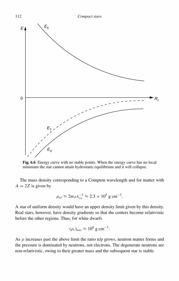
112 Compact stars
0 Rc
EK
EG
E
ET
Fig. 6.6 Energy curve with no stable points. When the energy curve has no localminimum the star cannot attain hydrostatic equilibrium and it will collapse.
The mass density corresponding to a Compton wavelength and for matter withA = 2Z is given by
ρrel ≈ 2m Pλ−3ce ≈ 2.3 × 10⁵ g cm−3.
A star of uniform density would have an upper density limit given by this density.Real stars, however, have density gradients so that the centers become relativisticbefore the other regions. Thus, for white dwarfs
(ρc)max ≈ 108 g cm−3.
As ρ increases past the above limit the ratio n/p grows, neutron matter forms andthe pressure is dominated by neutrons, not electrons. The degenerate neutrons arenon-relativistic, owing to their greater mass and the subsequent star is stable.

6.4 Stability of compact stars 113
decay
mnc2
0.78 MeV
mec2
mpc2
n
E
p+e
Fig. 6.7 Beta decay. Beta decay occurs when the rest mass energy of the neutronis greater than the combined energies of the electron and proton.
Thus
pn ≤ mnc = h
λcn
⇒ λcn ≈ h
mcnc≈ 1.3 × 10⁻¹³ cm = 1.3 fm
ρn,rel ≈ mn/λ3cn ≈ 7 × 10¹⁴ g cm−3.
The corresponding maximum density is then
ρmax ≈ few × 1015 g cm−3.
At these densities nuclear reactions are strong and they play an important role indetermining the structure of the neutron star. Consequently, the P(ρ) relation forneutron stars is not well modeled and there are great debates over its exact form.Figure 6.9 summarizes the stability of compact stars.

114 Compact stars
mnc2
mpc2
n
E
mec2 + ef
p+e
Fig. 6.8 Inverse beta decay (electron capture). Inverse beta decay occurs when thecombined energies of the electron and proton are greater than the rest mass energyof the neutron. In this case it is the Fermi energy that causes the inverse process.
6.5 Structure of neutron stars
6.5.1 Overview
At the high densities and pressures characteristic of neutrons stars, the internalstructure is quite interesting. At and just above the surface, where P = 0, ordinarymatter can exist and there is no degeneracy. Just below the surface, it is believedthat there is a relatively thin liquid layer, an ocean of non-relativistic degeneratematter. The interior is solid but the core may also be liquid as a result of a phasetransition. The unusual structure is the result of the high internal densities which inturn is the result of the extremely strong gravitational potential.
The characteristic radius of a neutron star can be obtained from the maximumdensity just derived
4
3ρmax R3
c ≈ 1 M
⇒ Rc ≈ 7 × 105 cm.

6.5 Structure of neutron stars 115
M/M
2
1
ρ
(g cm−3)
white dwarfs
neutron stars
black holes
1010 1015105
Fig. 6.9 Stability regimes for white dwarfs and neutron stars. The solid curvesindicate regions of stability. The dashed curves represent regions of instability forwhite dwarfs and neutron stars.
For real stars, with density gradients
8 < RNS < 20 km.
The surface gravity is then given by
gN = G M
R2≈ 1014 cm s−2.
Compare that to the Earth where g ≈ 103 cm s−2.
6.5.2 Liquid layer
The liquid surface is the result of relatively low densities in the outer regions ofthe neutron star. Here, there are still plenty of non-relativistic electrons and protonsand few neutrons. The situation is favorable (more later) for a liquid state when

116 Compact stars
ρ < 106 g cm−3. We can get an approximate depth scale for the neutron star oceanusing the following equilibrium equation
dP
dz= gρ (181)
which is just the equation of hydrostatic equilibrium where z is the depth. Theequation of state for neutron stars is given by
P ≈ 1013ρ5/3 = kρ5/3 (182)
as one would expect for a degenerate non-relativistic star. Substituting (145) into(144) yields
dz = 5
3ρ−1/3 k
gdρ. (183)
With the boundary condition ρ(z = 0) = 0 we get
z = 5
2
k
gρ2/3 for (ρ < 106 g cm−3)
⇒ z = 25 meters
(ρ
106 g cm−3
)2/3
. (184)
We see that the liquid surface layer has a characteristic depth of ≈ 25 meters.
Why is the surface layer liquid?
In the outer regions of the neutron star the nuclei are surrounded by a sea of electrons(Fig. 6.10). The electrons are bound to the nuclei with an energy
Ec ≈ − Ze2
ri≈ −
(4
3
)1/3
Ze2n1/3. (185)
At high densities the binding energy is high and the particles form a crystal lattice.At lower densities the thermal energies of the particles can partially break down thelattice and form a liquid. The parameter that controls when that happens is given by
Γ = Ec
kT. (186)
Computer simulations show that when Γ < Γm ≈ 150, matter is liquid. The meltingtemperature Tm can then be defined by combining (185) and (186)
Tm = Ec
kΓm≈ 103ρ1/3 Z5/3 K for A = 2Z
⇒ Tm = 3 × 10⁷
(ρ
106 g cm−3
)1/3
(187)
for Z ≈ 30.

6.5 Structure of neutron stars 117
e−
e−
e−
e−
e−
e−
e−
e−
e−
e−
e−
e−
+Ze
+Ze
+Ze
+Ze
+Ze
+Ze
Fig. 6.10 The liquid layer. The ions are shown as circles. They are imbedded in asea of electrons.
The internal temperature of a neutron star evolves with time so that
Tm > 108 K t < 103 years
Tm < 107 K t > 106 years.
According to (187) only a thin layer can be liquid after about a million years. Thatliquid has an estimated thickness of 10–100 meters. A solid crust forms below theocean.
6.5.3 The crust
In the outer crust, electron capture alters the composition according to
e− + (Z , N ) → (Z − 1, N + 1) + ν.

118 Compact stars
E
N
F
∋
Fig. 6.11 Electron capture brought on by degeneracy. The plot shows bindingenergies for nuclei of a fixed atomic mass. The presence of a biasing Fermi energyallows electron capture to occur to the right of the minimum.
Consider the plot of binding energies for nuclei of a fixed atomic mass in Fig. 6.11.Electron capture should not be possible to the right of the minimum. However, thehigh Fermi energies allow this to happen.
As the density increases with depth there is a corresponding increase in the Fermienergy, εF . At high enough Fermi energies of εF ≈ 20 MeV and ρ ≈ 1012 g cm−3
neutrons begin to drip out of the nuclei according to
(Z , N ) → (Z , N − 1) + n.
Thus, the outer crust has an altered composition of electrons and nuclei while theinner crust is a mixture of neutrons, nuclei and electrons.
6.6 Pulsars 119
6.5.4 The core
In the core the density approaches ρ ≈ 2.8 × 10¹⁴ g cm−3, at which point the nucleiare merging together to form a liquid core. This liquid consists of free neutrons,protons and electrons. At this point the Fermi energies are approaching 100 MeV,which is the rest mass energy of a muon. At the very center muons become a partof the mixture. For T < Tc ≈ 109−10K, free neutrons in the crust and in the coreform a neutron superfluid. Free protons in the core form a superconductor. Thesuperfluid represents flow without viscosity while superconductivity representsenergy conduction without losses.
6.6 Pulsars
Pulsars, as the name suggests, emit repeated pulses of radiation. The frequency ofpulsation is rapid ranging from milliseconds to seconds of time. The pulse frequencyis also very regular. The combination of rapid pulsation and regularity is a severeconstraint on the physics of these objects. There are two possibilities. Pulsars areeither dynamical pulsators (they contract and expand periodically like pulsatingvariable stars) or rapidly rotating objects.
The dynamical timescale for a stellar oscillation is given by
tdyn ≈ (24Gρ)−1/2
which is related to the free fall time. The period of oscillation must exceed thedynamical timescale, otherwise the star is destroyed.
P > tdyn = 446√ρ
seconds.
If we use a typical period for a pulsar (say that of the Crab nebula) we can derive alower limit on the density of the star.
ρ >
(446
0.033 s
)2
≈ 2 × 10⁸ g cm−3
which is just above the maximum density of a white dwarf. For faster pulsars, whitedwarfs can be ruled out.
In the case of rotation
acent = Ω2 R agrav = G M
R2
and for the star to be stable against disruption
Ω2 R =(
2
P
)2
R <G M
R2
⇒ (2)2 P−2 <G M
R3= 4
3Gρ

120 Compact stars
P >
(3
Gρ
)1/2
= 1200√ρ
⇒ ρ >
(1200
P
)2
= 1.3 × 10⁹ g cm−3.
The density has to be greater than ≈ 109 g cm−3, especially for the faster millisecondpulsars. This range of densities completely eliminates white dwarfs as candidates.Thus it seems that regardless of whether pulsars are oscillating or rotating they areprobably neutron stars. So which is it? Are they oscillating or rotating?
The periods of pulsars can be measured so accurately that it is possible to measurevery small changes in pulse periods. In the case of the Crab pulsar
P = 0.03342 . . . s
P = 2.5 × 10⁻¹² > 0
⇒ P
P= 2650 years.
The deceleration timescale is 2650 years. All pulsars for which the decelerationtimescales have been measured have positive P . That is, they all slow down andincrease their periods.
If pulsars were oscillating sources their evolution would be determined by theVirial theorem. Since they are emitting radiation and since they have no internalheat generation their density should increase with time. But according to theseequations
Posc ∝ ρ−1/2
which predicts that the period should decrease with time, contrary to what is actuallyobserved.
A rotating star loses rotational energy as it radiates so that
d
dt
(I
2Ω2
)= ΩΩ I + Ω2
2
dI
dt< 0
if I ≈ constant. Thus
Ω < 0 ⇒ P > 0
as is observed.Pulsars are rapidly rotating neutron stars. We will discuss pulsars in more de-
tail later, when we have reviewed EM. The radiation pulsars give off contains somevery interesting physics as we will see in Section 9.6.

6.7 Further reading 121
6.7 Further reading
Clayton, D. D. (1984) Principles of Stellar Evolution and Nucleosynthesis, University ofChicago Press, Chicago, USA.
Frank, J., King, A., Raine, D. (2002) Accretion Power in Astrophysics, CambridgeUniversity Press, Cambridge, UK.
Glendenning, N. K. (1996) Compact Stars: Nuclear Physics, Particle Physics andGeneral Relativity, Springer-Verlag, Heidelberg, Germany.
Kaminker, A. M. (1995) The Physics of Neutron Stars, Nova Science Publishers,Hauppauge, NY, USA.
Riffert, H. (Ed) (1996) Matter at High Densities in Astrophysics, Springer-Verlag,Heidelberg, Germany.
Shapiro, S. L. and Teukolsky, S. A. (1983) Black Holes, White Dwarfs and Neutron Stars,John Wiley and Sons, New York, USA.


Part III
Electromagnetism
Observational astronomy is based on the detection of radiation emitted by astro-physical objects. All morphological and physical information about astrophysicalsources is derived from observation and analysis of the emitted radiation. Contin-uum radiation is a natural consequence of the principle that accelerating charges ra-diate. In this part of the book I will review and apply principles of electromagnetismto further our understanding of important astrophysical phenomena, demonstratingin the process that important radiation processes can be derived from the basic prin-ciple that accelerating charges radiate. To that end, I will develop the theory thatdescribes bremsstrahlung and synchrotron radiation. A theoretical understandingof these two radiation mechanisms allows us to interpret the emission of a widerange of objects, ranging from distant radio galaxies to nearby HII regions. Thespecific astrophysical topics covered in this part of the book include: the radiativeproperties of pulsars, dispersion and Faraday rotation of electromagnetic radiation,active binary star systems, accretion disks, supernova remnants, particle accelera-tion, cosmic rays and active galaxies.
123


Chapter 7
Radiation from accelerating charges
A proper interpretation of the radiation detected from astrophysical sources requiresus to understand why radiation occurs and what the main radiation mechanisms are.In this chapter I derive the Lienard–Wiechert (L–W) potentials, which form the basisfor describing radiating charges using basic principles of EM and relativity. TheL–W potentials are used to describe two of the most important continuum radiationmechanisms in astronomy, thermal bremsstrahlung and synchrotron radiation.
7.1 The Lienard–Wiechert potential
7.1.1 Scalar and vector potentials
Recall the vector relation
∇ · ( ∇ × a) = 0
from which we can define a vector potential such that
∇ · B = ∇ · ( ∇ × A) = 0
⇒ B = ∇ × A, (188)
where B is the magnetic field and A is the associated vector potential.Substituting (188) into Faraday’s Law (from Maxwell’s equations (242)–(245))
∇ × E = −1
c
∂
∂t( ∇ × A) = −1
c∇ × ∂ A
∂t,
where E is the electric field and φ is the associated scalar potential. But recall that∇ × ( ∇φ) = 0 which we are then free to add to the right-hand side
⇒ ∇ × E = −∇ ×[
1
c
∂ A∂t
+ ∇φ
]
⇒ E = −1
c
∂ A∂t
− ∇φ. (189)
125

126 Radiation from charges
Generalizing this result
A′ = A + ∇Ψ
φ′ = φ − 1
c
∂Ψ
∂t,
These equations represent gauge transformations. The gauge transformations giveus mathematical flexibility for solving various EM problems. They are useful be-cause they do not change the underlying physics. A particularly useful gauge fordealing with radiation is given by the Lorentz condition
∇ · A − 1
c
∂φ
∂t= 0. (190)
Let us now substitute (188) and (189) into Coulomb’s and Ampere’s Laws (seeMaxwell’s equations (242)–(245))
⇒ −∇2φ − 1
c
∂
∂t( ∇ · A) = 4ρe (191a)
∇ × ( ∇ × A) = 4
cje − 1
c∇ ∂φ
∂t− 1
c2
∂2 A∂t2
. (191b)
Combining (190) and (191) we obtain
2
(φ
A)
= −4
(ρe
je/c
). (192)
This is known as the inhomogeneous wave equation where
2 ≡ ∇2 − 1
c2
∂2
∂t2.
It is possible to solve (192) with the help of Green’s function.
7.1.2 Green’s function solution
The first step is to solve the special case:
2G(x, t ; x ′, t ′) = 4(x − x ′)(t − t ′) (193)
for G, then
φ(x, t) =∫
G(x, t ; x ′, t ′)ρe(x ′, t ′) dx ′ dt ′ (194a)
A(x, t) =∫
G(x, t ; x ′, t ′)je(x ′, t ′)
cd3x ′ dt ′. (194b)

7.1 The Lienard–Wiechert potential 127
The solution to (193) is given by
Gret = (t ′ − (t − |x − x ′|/c))
|x − x ′| (195)
so that (194) becomes
φ(x, t) =∫
[t ′ − (t − |x − x ′|/c)]
|x − x ′| ρe(x ′, t ′) d3x ′ dt ′
A(x, t) =∫
[t ′ − (|x − x ′|/c)]
|x − x ′|jec
d3x ′ dt ′.
For t ′ = t − |x − x ′|/c, the retarded time, we have
φ(x, t) =∫
ρe(x ′, t ′)|x − x ′| d3x ′ (196a)
A(x, t) = 1
c
∫ je(x ′, t ′)|x − x ′| d3x ′. (196b)
These are known as the retarded potentials.
7.1.3 The L–W potentials
Consider a single charge q moving on a trajectory r (t)
⇒ ρe = q[x − r (t)
](197a)
j e = qv[x − r (t)
]. (197b)
Then, in terms of the preceding approach[ρe(x ′, t ′)j e(x ′, t ′)/c
]=
∫ [q
qv(τ )/c
](x ′ − r (τ ))(τ − t ′) dτ.
Substituting into (196) and integrating over x ′
φ(x, t) =∫ ∫
q(x ′ − r (τ ))
|x − x ′| (τ − t ′) d3x ′ dτ
which is nonzero only for x ′ = r (τ )
⇒ φ(x, t) =∫
q(τ − t ′)|x − r (τ )| dτ . (198)

128 Radiation from charges
Similarly
⇒ A(x, t) =∫
qv(τ )/c
|x − r (τ )| (τ − t ′) dτ. (199)
Now let us define R(τ ) ≡ x − r (τ )
⇒ t ′ = t − |x − x ′|/c = t − |x − r (τ )|/c (200)
t ′ = t − R(τ )/c. (201)
Now let τ ′ ≡ τ − t ′ = τ − t + R(τ )/c
⇒ dτ ′ = [1 + R(τ )/c] dτ. (202)
After some manipulation
dτ
R(τ )= dτ ′
R(τ ) − R(τ ) · v(τ )/c. (203)
Substituting (203) into (198) and (199)(φ(x, t)A(x, t)
)=
∫ (q
qv(τ )/c
)(τ ′) dτ ′
R(τ ) − R(τ ) · v(τ )/c. (204)
Equation (204) is nonzero only for τ ′ = 0 so
φ(x, t) = q
R(τ ) − R(τ ) · v/c
]ret
(205a)
A(x, t) = q v(τ )/c
R(τ ) − R(τ ) · v/c
]ret
(205b)
where ]ret indicates that quantities are evaluated at the retarded time, that is,for
τ = t − R(τ )/c. (206)
Equations (205) and (206) represent the Lienard–Wiechert potentials.
7.2 Electric and magnetic fields of a moving charge
The E and B fields can be evaluated according to
E = −∇φ − 1
c
∂ A∂t
and B = ∇ × A. (207)

7.2 Fields of a moving charge 129
θt
(t − τ)
|R(τ)| = c(
t − τ)
R(τ
) −
(t −
τ)v
= R
t
v
Fig. 7.1 Trajectory of a charge moving at constant velocity.
Now, from (206)
∂τ
∂t= 1
1 + R/c= 1
1 − R · v/c= 1
κ. (208)
Combining (207), (208) and (205)
E = q
(R − R · v/c)3
[(1 − v2
c2
) (R − Rv
c
)+
Rc2
×[(
R − Rvc
)× v
]]
(209)B = R × E .
Note that the first term in (209) ∝ 1/R2 and yields the Coulomb field. The secondterm ∝ 1/R and represents the Radiation field.
7.2.1 Moving charge at constant velocity
When v = 0 only Coulomb fields are possible. From Fig. 7.1
R −R · v
c= Rt
(1 − v2
c2sin2 θt
)1/2
=[| Rt |2 −
∣∣∣∣ Rt × vc
∣∣∣∣2]1/2
. (210)
For a proof see Shu (1992). Combining (207), (209) and (210)
⇒ E = q(1 − (v2/c2)) Rt
(| Rt |2 − | Rt × (v/c)|2)3/2and B = v
c× E . (211)

130 Radiation from charges
v v=0
Decelerated Charge
Fig. 7.2 The fields of a decelerating charge. A charge is moving initially atconstant speed v. It decelerates instantly to v = 0. Portions of the resulting E fieldsare shown.
Special cases
v = 0 → E = q
R2t
r
v ⊥ R → E = γ q
R2t
r
v ‖ R → E = 1
γ 2
q
R2t
r .
A qualitative picture based on (211) is shown in Fig. 7.2. Inspection of Fig. 7.2shows that when a moving charge suddenly stops, corresponding to an instantaneousacceleration, the static fields form two separate regimes. Causality demands thatthe fields associated with the two regimes be connected, as shown. Given the finitespeed of light, an external observer first sees the initial field associated with themoving charge. After a finite amount of time, corresponding to the time it takes forthe field of the stationary charge to reach the observer, a discontinuity in the E andB fields sweeps over the observer. This discontinuous field is the EM wave asso-ciated with the acceleration of the charge. Note that the E field lines along the dis-continuity are orthogonal to the direction of propagation and that the discontinuity

7.2 Fields of a moving charge 131
propagates at the speed of light, both characteristics of propagating EM radiation.Causality demands that accelerating charges radiate.
7.2.2 Radiation from accelerating charges – the far zone
Let us now investigate the second term in (209). In the far field, R = kx .
⇒ E = q
xc2κ3
k ×
[(k − v
c
)× v
](212)
B = k × E .
For v/c 1 → | E | = (q|v| sin θ )/xc2.For v/c ≈ 1 → κ = 1 − (k · v)/c ≈ 1 − cos θ , demonstrating that there is
relativistic beaming around θ ≈ 0.
7.2.3 Angular distribution of radiation
Recall that
dP
dΩ= x2 × | S|︸︷︷︸
Poynting Vector
= c
4(x | E |)2. (213)
Define
g = 1
κ3
k ×
[(k − v
c
)× v
](214)
with the help of Fig. 7.3, such that, from (212), (213) and (214)
dP
dΩ= q2|g|2
4c3.
Expanding the double product in (212)
g = 1
κ3
[(k · v)
(k − v
c
)− κ v
]
⇒ g · g = g2 = 1
κ4|v|2 + 2
κ5(k · v)
(v · v
c
)− 1
κ6
(1 − v2
c2
)(k · v)2 (215)
where we have used κ = 1 − (k · v)/c. We also note that
k · vc
= v
ccos θ
k · v = |v|(sin θ cos φ sin i + cos θ sin φ cos i)
v · vc
= |v|vc
cos i. (216)

132 Radiation from charges
z
x
y
kv
v
i
.
^
^
^
^
Fig. 7.3 Definition of coordinate system used to describe radiation patterns.
Armed with (215) and (216), two special cases can now be described.
Case 1 (‖v)
v ‖ v(i = 0) ⇒ k · vc
= v
ccos θ and k · v = |v| cos θ and v · v
c= |v|v
c.
Substitute into (215)
⇒ g2
|v|2 = sin2 θ
(1 − (v/c) cos θ )6.
The radiation pattern, corresponding to this equation, is shown in Fig. 7.4.
Case 2 ( ⊥v)
v ⊥ v(i = 90) ⇒ k · vc
= 0 and k · v = |v|(sin θ cos φ) and v · vc
= 0
⇒ g2
|v|2 =(
1 − v
ccos θ
)−4−
(1 − v2
c2
) (1 − v
ccos θ
)−6sin2 θ cos2 φ.
The radiation pattern, corresponding to this equation, is shown in Fig. 7.5.

7.2 Fields of a moving charge 133
v/c << 1
v, v v, v
v/c < 1 ~
Fig. 7.4 Radiation pattern when v ‖ v.
v v
v v
v/c << 1 v/c < 1 ~
Fig. 7.5 Radiation pattern when v ⊥ v.
7.2.4 Total emitted power
We can obtain an expression for the total power emitted by the radiating charge ifwe evaluate the following integral∫
dP
dΩ
dt
dτdΩ
where all angles are evaluated at time τ
⇒ P =∫
q2|g|24c3
κ sin θ dθ dφ.
Substituting into (215) and identifying |v|β sin i = |v × v/c| and after somemanipulation
Pem = 2e2
3c3γ 6[|v|2 − |v × v/c|2]. (217)
These equations describe the radiated power of a moving charge. Now we are in agood position to describe specific radiation mechanisms because (217) tells us that

134 Radiation from charges
the only thing we need to specify is the trajectory of the charge (its velocity andacceleration). As we will see it is the trajectory which defines radiation mechanisms.As examples, I will now describe two of the more important continuum radiationmechanisms in astrophysics, thermal bremsstrahlung and synchrotron radiation.
7.3 Further reading
Jackson, J.D. (1998) Classical Electrodynamics, John Wiley and Sons, New York, NY,USA.
Rybicki, G. B. and Lightman, A. P. (1985) Radiative Processes in Astrophysics, JohnWiley and Sons, New York, NY, USA.
Shu, F. H. (1992) The Physics of Astrophysics: Radiation, University Science Books, MillValley, CA, USA.
Tucker, W. H. (1975) Radiation Processes in Astrophysics, MIT Press, Cambridge, MA,USA.
Zhelezniakov, V. V. (1996) Radiation in Astrophysical Plasmas, Kluwer AcademicPublishers, Dordrecht, The Netherlands.
Chapter 8
Bremsstrahlung and synchrotron radiation
8.1 Bremsstrahlung
A thermal plasma in which the ionized particles follow a Maxwell–Boltzmanndistribution will undergo Coulomb interactions. The Coulomb forces cause thecharged particles to accelerate during the interactions (collisions) so that the parti-cles give off radiation. In this chapter we will study the acceleration of electrons ina thermal plasma and determine the characteristics of the emitted radiation usingequation (217).
8.1.1 Single particle collisions
We begin by considering the interaction of a free electron with a free ion, as shownin Fig. 8.1.
me|x | = Zi e2
b2 + v2t2and v ⊥ v v
c 1.
Substituting this into (217) yields
P = 2e2
3c3|v|2 = 2Z2
i e6
3m2ec3
1
(b2 + v2t2)2. (218)
Integrating over the entire collision
Ptot =∫
P(t) dt = 2e2
3c3
∫|vt |2 dt.
This integral has been expressed in the time domain. It can also be expressed in thefrequency domain if we recall Parseval’s theorem, namely∫ ∞
−∞|vν |2 dν =
∫ ∞
−∞|vt |2 dt.
135

136 Bremsstrahlung and synchrotron radiation
x
e v
b
θ
i-Z e
Fig. 8.1 A single particle collision. An electron, of velocity v, incident on an ion ofcharge Z is deflected by the Coulomb interaction. The impact parameter is shownas the distance of closest approach (b). The deflection angle is θ .
where
|vν | =∫
|vt | e2iνt dt. (219)
Thus ∫Pt dt =
∫Pν dν
⇒ Ptot = 2e2
3c3
∫ ∞
−∞|vν |2 dν = 4e2
3c3
∫ ∞
0|vν |2 dν. (220)
The differential form of (220) represents the frequency spectrum resulting fromone encounter
Pν = 4e2
3c3|vν |2 dν. (221)
Combining (219) and (221)
Pν = 4e2
3c3
[∫|vt |2 e2iνt dt
]2
. (222)
Combining (218) and (222)
Pν = 4e6 Z2i
3m2ec3
[
bv
]2e−4|ν|b/v. (223)

8.1 Bremsstrahlung 137
Equation (223) represents the single particle spectrum resulting from a singlecollision.
8.1.2 Radiation from an ensemble of particles
In reality we must consider the effect of many collisions. Since each collisiondepends on velocity we must know the velocity distribution of the particles in theplasma. For a thermal plasma that is given by the Maxwell–Boltzmann distribution.What we need to do is to integrate (223) over all velocities and all possible impactparameters. Thus
Pν =∫ ∞
vmin
[ne f (v)4v2 dv]
[42 Z2
i e6
3m2ec3v2
] ∫ ∞
bmin
e−4|ν|b/v 2b db
b2
where f (v) is usually a Maxwellian, in which case this simplifies to
Pν = ne
(2me
kT
)1/2 (83 Z2
i e6
3m2ec3
)I (224)
where
I =∫ ∞
xmin
e−x dx∫ ∞
ζmin
e−ζ
ζdζ
where
ζmin ≡ 4νbmin
vand xmin ≡ mev
2min
2kT.
For xmin we require (1/2)mev2min = hν
xmin = hν
kT. (225)
For bmin we require bminmev ≈ h (QM limit) so that
bmin = h
mev(226)
ζmin = 4νh
mev2.
Combining (224), (225) and (226) yields
Pν =∫ ∞
hν/kTe−x E1(ζmin) dx . (227)

138 Bremsstrahlung and synchrotron radiation
P
νν
n
P -hν/kT
h =kT
=E (1) e1
Fig. 8.2 Theoretical bremsstrahlung spectrum. The radiation from a single particlehas this spectrum. The fall-off is determined by the thermal energy of the particle.
For
hν
kT 1 ⇒ Pν ≈ E1(1) e−hν/kT .
For
hν
kT 1 ⇒ Pν ≈ ln
[γ
(me Z2
i e4
2h2hν
) (me Z2
i e4
2kT h2
)3/2]
− 3
2γ
where
γ = −∫ ∞
0ln x e−x dx .
The latter is a slowly varying function, therefore the overall spectrum can be approx-imated according to Fig. 8.2: This, with (227), represent a thermal bremsstrahlungspectrum. These spectra are characteristic of HII regions, supernova remnants andgalaxy clusters.
8.2 Synchrotron radiation
In the presence of a magnetic field, charged particles gyrate about the magneticfield. The gyration results in continuous circular acceleration so that the particlesradiate. In this section we will describe the total power and frequency spectrum of(a) a single gyrating particle and (b) an ensemble of particles. These results will beapplied to astrophysical sources.

8.2 Synchrotron radiation 139
a
v
B0
Fig. 8.3 Definition of pitch angle.
8.2.1 Total power
In the presence of a magnetic field a charged particle experiences a Lorentz force
d
dτ(γ mv) = q
( vc
× B0
)(228)
Rearranging
dvdτ
= v × zωB and ωB = q B0
γ c(229)
which has the solution
r (τ ) = zvzτ + vxy
ωB(x cos ωBτ + y sin ωBτ )
where
vz = v · B0
B0and vxy =
√v2
x + v2y = v × B0
B0
for B0 = B0 z. Letting cos α = v · B0/vB0 ⇒ R = (v/ωB) sin α. The angle α isknown as the pitch angle and is defined in Fig. 8.3. These descriptions of theparticle trajectory can be used to determine the radiation characteristics of theparticle through (217). The latter can be cast into a more convenient form
Pem = 2q2
3c3γ 4(a2
⊥ + γ 2a‖). (230)

140 Bremsstrahlung and synchrotron radiation
B0
∆θ
∆θ
Fig. 8.4 Beamed radiation from a gyrating electron. The electron is moving towardthe observer at that particular instant.
Comparing (229) and (230)
a⊥ = ωBv sin α and a‖ = 0.
Substituting into (230)
Pem = 2e2
3c3γ 2 e2 B2
0
m2ec2
v2 sin2 α for electrons.
Why can we ignore protons? Because Pem scales as 1/m4 and protons are 1800times more massive than electrons. Simplifying this equation
⇒ Pem = 2β2γ 2cσT UB sin2 α
where σT is the Thomson cross-section and UB = B20/(8). For an isotropic prob-
ability distribution
〈Pem〉 = 4
3β2γ 2cσT UB
where 〈sin2 α〉 = 2/3. For an ensemble of particles 〈Pem〉 = 〈P〉
⇒ 〈P〉 = 4
3β2γ 2cσT UB (231)
which describes both emitted and received power.
8.2.2 The received spectrum
We will take the approach of examining the properties of the pulses emitted byultra-relativistic gyrating particles (Fig. 8.4). In terms of the retarded time τ
⇒ τ
P= θ
2≈ 1
2γ.

8.2 Synchrotron radiation 141
γ3ωB
P(t)
2π/ωB2π
t
Fig. 8.5 Pulsed radiation from gyrating electron.
In terms of the observer’s time, recall
dt
dτ= 1 − β cos θ ≈ 1 − β + (θ )2
2≈ 1
γ 2(γ 1)
⇒ t
P= 1
2γ 3⇒ ν ≈ γ 3ωB .
Using standard pulse analysis we can predict emission at ω = ωB → γ 3ωB
(Fig. 8.5). Now let us define ωL = γωB = eB0/mec and let ν = ω/2
⇒ 〈Pν(γ )〉 = 4
3β2γ 2cσT UBφν(γ ) (232)
such that∫ ∞
0 φν(γ ) dν = 1. From an ensemble of particles at energy γ we wouldexpect a discrete spectrum with a basic period of
2
ωB= γ
νL.
But
νL = eB0
2mec≈ 20−30 Hz.
In astrophysical sources the basic period is too low to be detectable. In a typicalastrophysical spectrum where γ ≈ 104
⇒ νB = γ −1νL = 2 × 10⁻³ Hz
the spacing of the harmonics. The spectrum, in practice, is continuous, as shown inFig. 8.6.
8.2.3 Spectrum of a power-law energy distribution
Consider an energy distribution of electrons defined by
n(γ ) dγ → mec2γ − mec2(γ + dγ ).

142 Bremsstrahlung and synchrotron radiation
φνlog
ν=γ ν2L
ν
log ν2
e-
2Lν/γ ν1/3
Fig. 8.6 Synchrotron spectrum of a single electron. The gyrating electron emitsradiation that is characterized by the spectrum shown. The fall-off frequency isdetermined by the energy, γ , of the electron.
slope −(p − 1)/2
log jν log jν
log v log v
ν-0.75
ν-0.1
synchrotron
bremsstrahlung
Fig. 8.7 Synchrotron spectrum of an ensemble of electrons. A power-law energydistribution of electrons yields a power-law synchrotron spectrum. The latter canbe thought of as the superposition of individual electron spectra, scaled by the elec-tron energy. The slope of the resulting spectrum is shown in terms of the power-lawindex of the energy distribution. The plot on the right shows typical spectra asso-ciated with synchrotron and bremsstrahlung radio sources. The markedly differentslopes of the two spectra allow astronomers to differentiate between thermal andnon-thermal sources.
With (232) we can define a volume emissivity
ρ jν =∫ ∞
1〈Pν(γ )〉n(γ ) dγ. (233)
Empirical evidence indicates that
n(γ ) dγ = n0γ−p dγ = n0γ
−2.5 dγ. (234)

8.3 Further reading 143
Now substitute (232) and (234) into (233), letting
φν(γ ) → (ν − γ 2νL )
and let β ≈ 1, ν ′ = γ 2νL and integrate to get
ρ jν = 2
3cσT n0UBν−1
L
(ν
νL
)−(p−1)/2
. (235)
The basic result is independent of actual shape of φν . We can define a luminosityLν by integrating (235) over the volume of the source
Lν =∫
Vρ jν dV ∝ ν−(p−1)/2. (236)
The net result is a power-law spectrum, as shown in Fig. 8.7.
8.3 Further reading
Jackson, J. D. (1998) Classical Electrodynamics, John Wiley and Sons, New York, NY,USA.
Pacholczyk, A. G. (1970) Radio Astrophysics. Nonthermal Processes in Galactic andExtragalactic Sources, Freeman, San Francisco, USA.
Rybicki, G. B. and Lightman, A. P. (1985) Radiative Processes in Astrophysics, JohnWiley and Sons, New York, NY, USA.
Shu, F. H. (1992) The Physics of Astrophysics: Radiation, University Science Books, MillValley, CA, USA.
Tucker, W. H. (1975) Radiation Processes in Astrophysics, MIT Press, Cambridge, MA,USA.
Verschuur, G. A. and Kellerman, K. I. (1988) Galactic and Extragalactic RadioAstronomy, Springer-Verlag, Berlin, Germany.
Zhelezniakov, V. V. (1996) Radiation in Astrophysical Plasmas, Kluwer AcademicPublishers, Dordrecht, The Netherlands.

Chapter 9
High energy processes in astrophysics
Unlike the black-body radiation that characterizes stars and planets, thebremsstrahlung and synchrotron processes are tracers mainly of high-energy phe-nomena. The former often traces regions of hot ionized gas, the latter traces non-thermal matter consisting of relativistic particles. As we will see later, both processesare associated with supernova remnants and accreting neutron stars. I now examinethese phenomena in more detail.
9.1 Neutron stars
When matter accretes onto a neutron star, the energy gained by a particle (assumea proton) is just the potential energy per particle at the neutron star surface
Up = −G Mm p
R≈ 2 × 10⁻⁴ ergs ≈ 0.1 m pc2.
Thus, a thermalized particle at the surface has a temperature of
kT ≈ 108 eV ≈ 100 MeV.
In principle particles can radiate γ rays. However, the Eddington limit (more detailslater) sets a maximum luminosity of
L = 4R2σ T 4 ≈ 1037 erg s−1
⇒ T ≈ 107 K ⇒ kT ≈ 1 keV.
Matter at this temperature is a fully ionized plasma so that collisions are mediatedby Coulomb interactions. This, of course, is a recipe for thermal bremsstrahlung.
As noted in the previous chapters, bremsstrahlung is characterized with a highenergy cut-off defined by,
hν ≈ kT .
144

9.2 Supernova remnants 145
Thus, for kT ≈ 1 keV → hν ≈ 1 keV. The accreting region should therefore emitto hundreds of electronvolts, consistent with their designation as UV and X-raysources.
We can contrast this with HII regions (kT ≈ 1 eV). In this case bremsstrahlungdoes not operate at the quantum limit and bmin ≈ Zi e2/mev
2. Comparing withthe quantum limit (189) we see that, in this case, bmin is larger by a factor ofZi e2/hv ≈ 4 × 10⁸. The photon energies are therefore smaller by a similar factor,yielding frequencies of order 1 GHz. The HII regions are known to be radio sources.
9.2 Supernova remnants
Supernovas leave behind a neutron star (sometimes a black hole). They also ejecta shell of material which is called a supernova remnant (SNR). Detection of 1 keVphotons from SNRs suggests that
kT ≈ 103 eV ⇒ T ≈ 107 K.
The bremsstrahlung process operates here too! Since it depends on ne as well as Tthe density can be evaluated once T is known. Typical values of ne are 0.1–10 cm−3,averaged over the SNR.
How much energy does it take to ionize this much gas?Consider a 10 pc SNR. Then
nekT Vsnr ≈ (10)(2 × 10⁻⁹)(3 × 10¹⁹)3
≈ 5 × 1050 ergs ⇒ blast energy!
Where does the energy come from?
ρv2
2≈ nekT ⇒ v ≈
√2kT
m p≈ 5 × 107 cm s−1
≈ 500 km s−1.
But the sound speed
cs ≈ 30 km s−1 ⇒ M ≈ 17 → supersonic.
The supersonic shock from the explosion heats the interior of the SNR.
9.2.1 Particle acceleration
Given the large amount of kinetic energy associated with SNRs, is it possible thatSNRs are the source of most of the relativistic particles in the Galaxy? At the Earthwe detect these particles as cosmic rays. From all sky radio surveys (see Fig. 8.7)

146 High energy processes
we know that the Galaxy is filled with cosmic rays because the radio emission isalmost entirely synchrotron.
Recall νc = eB
2mecγ 2.
For B = 5µG, γ = 2 × 10⁴ ⇒ ν = 3 GHz. At radio frequencies, synchrotron-emitting electrons are highly relativistic.
Observations of synchrotron emission in SNRs indicates that relativistic particlesare also present there. For SNRs to be the primary source of cosmic rays we needa mechanism that taps the blast energy of the SNR. That mechanism is known asdiffusive shock acceleration (see Gaisser, 1990).
To determine whether SNRs are plausible sources of cosmic rays we need toevaluate how much of an SNR’s energy is in the form of cosmic rays.
Minimum energy
Consider an SNR of volume V , containing a mixture of cosmic rays and magneticfields. The energy density of the magnetic field is simply
UB = B20
8. (237)
The energy density of the cosmic rays is a little more difficult to determine. Forelectrons
Ue = n0
∫ ∞
γmin
(γ mec2) γ −p dγ = n0mec2
2 − pγ
−(p−2)min [p > 2] (238)
requiring knowledge of the electron energy density distribution. But, from syn-chrotron theory, Pν ∝ n0 B−(p+1)/2
0 , so that
n0 = constant × B(p+1)/20 (239)
at a fixed frequency, ν, of observation.Combining (238) and (239)
⇒ Ue = constantB−(p+1)/20 at fixed ν (fixed γ ). (240)
The total non-thermal energy can now be expressed in terms of the magnetic fieldstrength
U = UB + kUe = UB + UC R
⇒ U ∝ B20 + B−(p+1)/2
0 (241)

9.2 Supernova remnants 147
Fig. 9.1 Minimum energy. The energy in particles and fields is plotted as a functionof B0. The curve has a well-defined minimum.
from (237) and (240) and where k = UC R/Ue (which can be estimated from obser-vations of cosmic rays at the Earth). A plot of (241) is shown in Fig. 9.1. Equation(241) has a minimum when
d
dB0(UC R + UB) = − (p + 1)UC R
2B0+ 2UB
B0= 0
⇒ UC R = 4
p + 1UB .
For p ≈ 2.5, UC R ≈ UB . There is an approximate balance between the cosmic rayand magnetic field energy densities. This balance is known as equipartition.
From this we see that the minimum energy can now be expressed as
Umin = (UC R + UB)min ≈ 2UC R ≈ 2UB .
The equipartition condition allows the calculation of B0 which yields UC R , UB andUmin . Regardless of assumptions about equipartition, Umin can always be calculated.The non-thermal energy curve for a SNR in the nearby galaxy, M33, is shown inFig. 9.2. Arguments based on equipartition have been used to estimate how muchcosmic ray energy resides inside SNRs. These calculations suggest
〈Umin〉 ≈ 5 × 1049 ergs
which is a substantial fraction of the blast energy (estimated to be ≈ 1051 ergs).On the basis of these numbers it seems plausible that SNRs convert a fair fraction
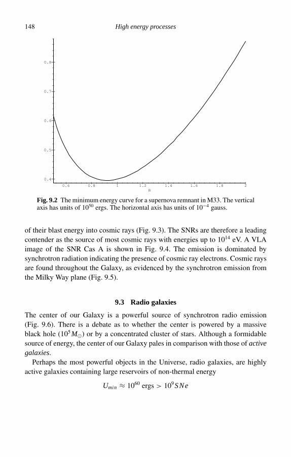
148 High energy processes
0.4
0.5
0.6
0.7
0.8
0.6 0.8 1 1.2 1.4 1.6 1.8 2B
Fig. 9.2 The minimum energy curve for a supernova remnant in M33. The verticalaxis has units of 1050 ergs. The horizontal axis has units of 10−4 gauss.
of their blast energy into cosmic rays (Fig. 9.3). The SNRs are therefore a leadingcontender as the source of most cosmic rays with energies up to 1014 eV. A VLAimage of the SNR Cas A is shown in Fig. 9.4. The emission is dominated bysynchrotron radiation indicating the presence of cosmic ray electrons. Cosmic raysare found throughout the Galaxy, as evidenced by the synchrotron emission fromthe Milky Way plane (Fig. 9.5).
9.3 Radio galaxies
The center of our Galaxy is a powerful source of synchrotron radio emission(Fig. 9.6). There is a debate as to whether the center is powered by a massiveblack hole (105 M) or by a concentrated cluster of stars. Although a formidablesource of energy, the center of our Galaxy pales in comparison with those of activegalaxies.
Perhaps the most powerful objects in the Universe, radio galaxies, are highlyactive galaxies containing large reservoirs of non-thermal energy
Umin ≈ 1060 ergs > 109SNe

9.3 Radio galaxies 149
log U
log
N(U
)
49 49.5 50 50.5 51
.2
.4
.6
.8
1
1.2
N(U)
Fig. 9.3 A histogram of minimum energies calculated for a sample of about50 SNRs in M33. The energy is in ergs. The sample is complete above logU ≈ 49.5.

150 High energy processes
Fig. 9.4 A VLA image of the SNR, Cas A. The observing frequency is 1.4 GHz.The radio emission is dominated by synchrotron radiation indicating that theSNR contains relativistic electrons gyrating in magnetic fields. Image courtesyof NRAO/AUI.
located hundreds of kiloparsecs from the power centers of these galaxies, theirnuclei. A VLA image of Cygnus A, a well-known radio galaxy, is shown in Fig. 9.7.
A simple light travel time argument illustrates that the relativistic particles fillingthese reservoirs must be accelerated in situ.
The lifetime of a relativistic particle is ultimately dependent on the rate at whichit loses energy (emits synchrotron radiation).
mec2 dγ
dτ= −Pem = −2β2γ 2cσT UB sin2 α
⇒ − γ
dγ /dτ= mec/γ
2σT UB sin2 α.

9.3 Radio galaxies 151
Fig. 9.5 The radio sky at 408 MHz. The grey-scale represents intensity of radioemission from the sky with black being most intense. The Galactic plane is horizon-tal in this representation. Although radio emission is evident across the whole skythere is a concentration of emission toward the plane and the center of the Galaxy.From: http://www.mpe.mpg.de/∼hcs/Cen-A/Pictures/galaxy-radio408mhz-2.gif.
Fig. 9.6 A VLA image of the Galactic center. The observing frequency is 1.4 GHz.The filamentary structures are not well understood but are believed to be relatedto violent activity at the Galactic center. Image courtesy of NRAO/AUI.

152 High energy processes
Fig. 9.7 A VLA image of the active galaxy Cygnus A. The observing frequencyis 1.4 GHz. The two outer lobes are intense sources of synchrotron emissionsuggesting that the lobes are filled with relativistic electrons and magnetic fields.The nucleus of Cen A is the relatively faint point source at the center of the image.Image courtesy of NRAO/AUI (Perley, R. C., Carilli, C. and Dreher, J.).
Typically, B = 10−5 G, γ ≈ 104 → τe ≈ 107 years. For γ = 106 → τe ≈ 105
years. But the light-travel-time for a distance of l ≈ 1025 cm ⇒ τc ≈ l/c ≈ 107
years. So, how is energy transferred in radio galaxies? The particles must be accel-erated within the lobes and perhaps all along the way from the nucleus to the lobes.If that is the case, there is no need for the particles to be completely transferred tothe lobes. The acceleration occurs in situ.
9.4 Galactic X-ray sources
As we have discussed earlier, rotation powers some objects such as pulsars. Inbinary stars, infalling matter can also power neutron stars and white dwarfs. Thelatter are called accretion powered sources. They are among the most powerfulsources in the Galaxy and emit much of their radiation in the high-energy part ofthe EM spectrum. They were discovered by the earliest X-ray telescopes (such asUhuru) and studied in great detail by subsequent X-ray and γ -ray satellites suchas Copernicus, Ariel 5, SAS-3, OSO-7.8, COS-B, HEAO-1, Einstein, EXOSAT,ROSAT, ASCA, XTE and Chandra. These X-ray sources are characterized by X-rayluminosities of Lx (2–10 keV) ≈ 1035–1037 erg s−1. Since they are always foundin binary star systems the source of the energy is believed to be mass transfer froma companion star to the compact star (white dwarf, neutron star, black hole) hencethe name X-ray binaries.

9.4 Galactic X-ray sources 153
9.4.1 The energy source
Matter falling onto a compact star represents the conversion of gravitational poten-tial energy into radiation. Thus, as discussed earlier,
Lx ≈ MG Mc
Rc= Mc2
(G Mc
c2 Rc
)= Mc2
(2Rs
Rc
)
where, Mc, Rc are the mass and radius of the compact object and Rs is theSchwarzschild radius of the compact object. For a white dwarf, Mc ≈ 1M, Rc ≈1 000 km. The efficiency of energy conversion is given by
≈(
G Mc
c2 Rc
)≈ 0.001
or about 0.1%. For neutron stars, Mc ≈ 1M, Rc ≈ 10 km
⇒ efficiency ≈ 0.1
or about 10%. For a black hole the efficiency is also about 10%. These numberscontrast with 0.7% for thermonuclear burning of hydrogen and 0.1% for burning ofheavier elements. Neutron stars and black holes are the most efficient astrophysicalengines known. In order for these engines to produce the observed X-ray luminosi-ties of Lx ≈ 1037 erg s−1 the required rate of mass accretion is M ≈ 10−9 M/yearfor a neutron star and M ≈ 10−7 M/year for a white dwarf.
9.4.2 Maximum luminosity/Eddington limit
It is no accident that X-ray binaries have a well-defined upper limit to their lumi-nosities. As compact stars accrete more matter they become more luminous. Theincreased radiation pressure opposes the gravitational infall of matter and even-tually an equilibrium is reached at the so-called Eddington luminosity. This canbe investigated quantitatively. We begin with the simplifying assumption that theinfalling matter is pure, fully ionized hydrogen. Then
Fg = −G Mcρ
r2= −G Mcnm p
r2
Fr = L
4r2cnσT spherical symmetry
where σT = 6.6 × 10⁻²⁵ cm2 is the Thomson cross-section and Fg and Fr are thegravitational and radiation forces respectively. An equilibrium is reached when
Fr = −Fg ⇒ L = L Edd = 4G Mccm p
σT= 1.3 × 1038
(Mc
M
)erg s−1.

154 High energy processes
9.4.3 Characteristic temperature
What would the surface temperature of the compact star have to be in order tothermally emit the required 1037 erg s−1? With
L = 4R2cσ T 4
c
and σ = 5.7 × 10⁻⁵ erg cm−2 degrees−4 s−1
T ≈ 107
(R
10 km
)−1/2
K → kT ≈(
R
10 km
)−1/2
keV.
Neutron stars and black holes are natural X-ray emitters. White dwarfs are naturalUV sources. The emission we have discussed thus far can be characterized as blackbody and originates in the compact accretion disks that form around the compact star(see Section 9.4.4 next). The black-body radiation is optically thick bremsstrahlung.These sources also emit optically thin bremsstrahlung and synchrotron radiation.
9.4.4 Mass transfer
We now investigate how matter is transferred onto the compact object.
Roche Lobe overflow
In Fig. 9.8, matter from one star spills over the equipotential surfaces that definethe potential of the two-body system.
Stellar winds
A variant of the above picture suggests that the mass-carrying wind of the evolvingstar is focused onto the compact object by the latter’s intense gravitational field(Fig. 9.9). Upper main-sequence stars have
Mwind ≈ 10−7−10−6 M/ year
⇒ Macc ≈ 0.1% of Mwind
⇒ Macc ≈ 10−9−10−10 M/year, which is adequate.
9.5 Accretion disks
Matter falling onto the compact star forms an accretion disk. How? The obser-vational evidence for white dwarfs comes in the form of cataclysmic variableswhere we see Doppler shifts from gas corresponding to Keplerian velocities at theRoche Lobe. In the case of neutron stars we observe X-ray binaries. The best caseis Hercules X-1 which shows evidence for a large precessing disk. A schematicrepresentation of the evolution of an accretion disk is shown in Fig. 9.10.

9.5 Accretion disks 155
Mc M0
Fig. 9.8 Potential surfaces of a binary star. The compact star is shown as Mc. Gasspills over from M0 to Mc.
Mc M0
Fig. 9.9 Focused wind in a binary star system. The stellar wind of the evolvingstar is focused by the gravitational field of the compact star, resulting in massaccretion.

156 High energy processes
Shock formation
Ring spreads becauseof viscocity > disk
Ring formation
Fig. 9.10 Formation of an accretion disk. The formation of an accretion disk occursin stages, beginning with the formation of a shock as the material piles up duringinfall, and ends with ring spreading into a disk because of gas viscosity.
r
z
^Mc
h
Fig. 9.11 Cross-section of an accretion disk. The parameters used to define thevertical structure of the disk are shown.
9.5.1 Disk hydrodynamics
Let us consider a steady-state axisymmetric thin disk (Fig. 9.11). We will brieflydiscuss the vertical structure of the disk. A description of the full structure of thedisk requires consideration of the equations of mass conservation, conservationof radial momentum, conservation of angular momentum and the conservation ofenergy, which is beyond the scope of this book.

9.5 Accretion disks 157
M (r + ∆r)
M (r)
E
E•
•
Fig. 9.12 Pressure gradients in an accretion disk.
Vertical structure
The vertical (z direction) scale length is defined as
h ≡ 1
ρ0
∫ ∞
0ρ(z) dz.
In order for the accretion disk to be in hydrostatic equilibrium
dP
dz= −ρgz = −ρ(z)
G M
r2
z
r
P = G M
r3
∫ ∞
0ρ(z)z dz ≈ G Mρh2
2r3(h
r
)2
= 2P/ρ
G M/r≈ 2
c2s
VP≈ c2
s
Vk.
Since cs Vk , we see that h/r 1. The accretion disk is very thin. Consequently
P
r G Mρ
r2.
The pressure gradients are very small in the radial direction (Fig. 9.12).
9.5.2 The emission spectrum of the disk
In order to determine the emission spectrum of the accretion disk we begin bycrudely estimating the rate of energy deposition per unit area, Q (Fig. 9.13).
Q2rr = M
[− G M
2(r + r )+ G M
2r
]= G M M
2r2r
⇒ Q = G M M
4r3.

158 High energy processes
<ν>Frequencyof peak
Area
Q = power/area
r
Q
Fig. 9.13 Functional dependence of Q, peak frequency and the area.
When viscosity is included (a form of energy transport)
Q = 3
8
G M M
r3.
The spectral signature of the accretion disk is the empirically determined Lν ∝ ν1/3
law. Let us see if we can model such a law theoretically. From the previous discussion
Q(r ) ∝ 1
r3.
Thus, for black-body emission
Q = σ T 4 ∝ 1
r3→ T ∝ r−3/4
and
νB B ≈ kT ∝ r−3/4
⇒ Lν = 2
∫r dr S(ν, r )∫ ∞
0S(ν, r ) dν = Q(r ) = Q0
r3.
Let us treat S(ν, r ) as a sharp function of frequency such that
S(ν, r ) ≈ Q0
r3
[ν − ν0
(r
r0
)−3/4]
.
9.6 Pulsars revisited 159
We are using a similar approach to that we used when discussing synchrotronemission.
Now, let us define
[ν − ν0
(r
r0
)−3/4]
≡ [ f (ν, r )]
so that
Lν ≈ 2
∫r
drQ0
r2 [ f (ν, r )]
= 2Q0
∫1
r2 (d f/dr )( f )
(d f
dr
)dr
= 2Q0
∫1
r2 (d f/dr )( f ) d f.
Now, from this
d f
dr= 3
4ν0r3/4
0 r−7/4 ∝ r−7/4
so that
Lν ∝(
r7/4
r2
)f =0
= (r−1/4) f =0.
Since f = ν − ν0 (r/r0)−3/4 = 0
⇒ r−3/4 ∝ ν → r−1/4 ∝ ν1/3.
So, finally
Lν ∝ ν1/3.
The accretion disks around neutron stars are characterized by this spectrum whichincorporates black-body radiation (at low frequencies), a ν1/3 law at intermediatefrequencies and a high-frequency bremsstrahlung fall-off (Fig. 9.14).
9.6 Pulsars revisited
In addition to being astrophysically interesting, pulsars also represent interestingapplications of what we have learned in previous chapters. The reason for the latteris that they have both static and radiation fields with a well-defined transition regionseparating the two EM regimes.

160 High energy processes
log Lv
log v
Lv ∝ v1/3
Lv ∝ v2
Lv ∝ e−hν/kT
Fig. 9.14 Emission spectrum of an accretion disk. The optically thick regime isshown as a dashed curve at low frequencies. The optically thin regime is shownas a solid line while the fall-off is shown as a dotted line.
Ω
Fig. 9.15 Aligned magnetic field. The B field is said to be aligned with the rotationaxis of the pulsar.
9.6.1 The radiation field
Neutron stars have intense dipolar magnetic fields which are anchored to the starand therefore rotate with it (Fig. 9.15). The rotating magnetic field is responsiblefor generating a strong static electric field as well as radiation. To see that a rotating

9.6 Pulsars revisited 161
magnetic field does radiate let us consider its rotation.
B = B0
(r
Rs
)−3
.
The rapid rotation of the B field ensures that at some radius, RL , the linear velocityof the B field must be that of light, that is when
Ω = c
RL.
Thus, inside RL we have v = rΩ < RLΩ = c and the fields are said to co-rotatewith the star. On the other hand, outside RL , v = rΩ > RLΩ > c and co-rotationis not possible. For r > RL the rotating B field must radiate away energy in ordernot to violate causality.
9.6.2 Radiated power
We can get an estimate of how much power must be radiated by examining theenergy density of the magnetic field at the light cylinder.
U ≈ B2
8= 1
8
[Bs
(RL
Rs
)−3]2
= B2s
8
R6s
R6L
.
From the definition of the Poynting vector
S = Uc
⇒ E ≈ −4R2LUc = 1
2B2
s R6s R−4
L c
= −1
2B2
s R6s Ω
4c−3.
Thus
d
dt
(IΩ2
2
)= IΩΩ = − B2
s R6s Ω
4
2c3.
So that,
Ω ∝ −Ω3
Ω ∝ t−1/2 if Ω Ωinitial
P ∝ t1/2
⇒ t = P
2P.

162 High energy processes
For the Crab pulsar t = 1300 years. The predicted age of the Crab pulsar is notfar from its known age (we know the Crab supernova went off in AD 1054, almost1000 years ago).
9.6.3 The Braking Index
It is conventional to characterize the spindown of a pulsar by the so-called BrakingIndex, n defined by
Ω = −kΩn
or
ΩΩ
Ω2= n.
For magnetic dipole radiation n = 3.
9.6.4 The static magnetic field
We can use these equations to estimate the magnetic field strength of the Crabpulsar.
B2 = − I Ωc3
R6s Ω
3= I
(2)2
P Pc3
R6s
B ≈ (P P)1/2 I 1/2c3/2
2R3s
≈ 3.3 × 10¹⁹(P P)1/2
(I
1045 g cm−3
)1/2 (R
10 km
)−3
.
For the Crab pulsar, for which P and P have been accurately measured,
B ≈ 3 × 10¹² G.
The range for typical pulsars is given by
1011 < B < 1013 G.
9.6.5 The static electric field
A rotating magnetic field (Fig. 9.16) will generate an electric field according to
E = vc
× Bwhere
|v| = RΩ.
A charged particle will accelerate along the E field and gain energy before leavingthe pulsar magnetosphere. The amount of energy gain for a particle of charge q is
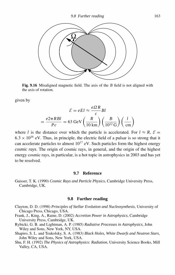
9.8 Further reading 163
Ω
Fig. 9.16 Misaligned magnetic field. The axis of the B field is not aligned withthe axis of rotation.
given by
E = eEl ≈ eΩ R
cBl
= e2R Bl
Pc= 63 GeV
(R
10 km
) (B
1012 G
) (l
cm
)
where l is the distance over which the particle is accelerated. For l ≈ R, E =6.3 × 10¹⁶ eV. Thus, in principle, the electric field of a pulsar is so strong that itcan accelerate particles to almost 1017 eV. Such particles form the highest energycosmic rays. The origin of cosmic rays, in general, and the origin of the highestenergy cosmic rays, in particular, is a hot topic in astrophysics in 2003 and has yetto be resolved.
9.7 Reference
Gaisser, T. K. (1990) Cosmic Rays and Particle Physics, Cambridge University Press,Cambridge, UK.
9.8 Further reading
Clayton, D. D. (1998) Principles of Stellar Evolution and Nucleosynthesis, University ofChicago Press, Chicago, USA.
Frank, J., King, A., Raine, D. (2002) Accretion Power in Astrophysics, CambridgeUniversity Press, Cambridge, UK.
Rybicki, G. B. and Lightman, A. P. (1985) Radiative Processes in Astrophysics, JohnWiley and Sons, New York, NY, USA.
Shapiro, S. L. and Teukolsky, S. A. (1983) Black Holes, White Dwarfs and Neutron Stars,John Wiley and Sons, New York, USA.
Shu, F. H. (1992) The Physics of Astrophysics: Radiation, University Science Books, MillValley, CA, USA.
Chapter 10
Electromagnetic wave propagation
So far we have assumed that the radiation we receive from astronomical sourcesis unaltered en route to the observer. However, in some cases this assumption isnot correct. I will now examine the dispersion of EM radiation and the relatedphenomenon of Faraday rotation, both of which are important at radio frequencies.
I begin with Maxwell’s Equations,
∇ · E = 4ρe (242)
∇ × E = −1
c
∂ B∂t
(243)
∇ × B = 4
cJ + 1
c
∂ E∂t
= −4
cρe V + 1
c
∂ E∂t
(244)
∇ · B = 0. (245)
Consider also the force law for charged particles
ρm∂ V∂t
= −ρe E − ρe
c( V × B). (246)
These equations describe the interplay between plasmas and EM waves.Consider a plasma with no large scale E and B fields and an EM wave passing
through it. The plasma sees oscillating E and B fields
E1 = E10 ei(k·r−ωt) B1 = B10 ei(k·r−ωt). (247)
The electrons in the plasma, being lighter, oscillate in response. We therefore lookfor electron velocity solutions of the form
V = V0 e−iωt . (248)
164

10.1 EM waves in an un-magnetized plasma 165
10.1 EM waves in an un-magnetized plasma
When B = 0,⇒ V × B = 0 (in (246)).
Combine ∇ × (243) and ∂/∂t (244) and (246), and eliminate ∂ Ve/∂t and B
⇒ −c ∇ × ( ∇ × E) = 4ρ2e
ρmcE + 1
c
∂2 E∂t2
.
Use identity ∇ × ( ∇ × E) = ∇( ∇ · E) − ∇2 E .Define ω2
e = 4ρ2e /ρm = 4nee2/me – Plasma Frequency
⇒ c∇2 E = ω2e
cE + 1
c
∂2 E∂t2
. (249)
Consider the 1-D case
c∂2 E
∂x2= ω2
e
cE + 1
c
∂2 E
∂t2. (250)
Look for plane wave solutions described by (247)
−ck2 E = ω2e
cE − ω2
cE
⇒ E
(ω2
c− ck2 − ω2
e
c
)= 0
⇒ ω2 = ω2e + c2k2
which is the Dispersion Relation. We can now define the index of refraction, thephase speed and the group velocity.
Index of Refraction
η = ck
ω=
√ω2 − ω2
e
ω=
√1 − ω2
e
ω2
ωe < ω → 0 < η < 1
ωe = ω → η = 0
ωe > ω → η = imaginary → reflection and absorption
Phase Speed
Vp = ω
k= 1
k
√ω2
e + k2c2 (251)
ωe > 0 → Vp > c
ωe = 0 → Vp = c (vacuum)
ωe kc → Vp = ωe/k

166 Electromagnetic wave propagation
Group Velocity
Vg = ∂ω
∂k= c2k√
ω2e + c2k2
(252)
ωe > 0 → Vg < c
ωe = 0 → Vg = c
ωe ck → Vg = kc2/ωe → 0.
10.1.1 Dispersion measure
To relate these to astronomical phenomena, let us consider observations of radiofrequency signals emitted by pulsars. A pulse is a wave packet and its propagation istherefore characterized by its group velocity. Dispersion has the effect of spreadingthe pulse such that different pulse frequencies will arrive at different times. Considera pair of observations made at frequencies ω1 and ω2. The arrival times are thereforet1 and t2 and are governed by the phase velocity. The difference in arrival times is
t = t1 − t2 = l
V1− l
V2(253)
where V1 and V2 are the phase velocities at ω1 and ω2 and l is the distance to thesource. Rearranging (251)
Vp = c√1 − (
ω2e/ω
2) . (254)
Normally, ω ωe so that (254) becomes
Vp ≈ c
1 − 12
(ω2
e/ω2) . (255)
Inserting (255) into (253), cross multiplying and neglecting high order terms in thedenominator, yields
t ≈ lω2e
2c
[1
ω21
− 1
ω22
](256)
⇒ t ≈ 2e2
mec
[1
ω21
− 1
ω22
]nel = 1.35 × 10⁻³
[1
ν21
− 1
ν22
]DM seconds.
(257)
The quantity nel is referred to as the dispersion measure and is often denoted asDM. Since ne is normally a function of l (257) is generalized so that
DM =∫ l
0ne dl ′ cm−2. (258)

10.2 EM waves in a magnetized medium 167
z
x
y
B0, k
E1
B1
^
^
^
^
^
^^
^V
Fig. 10.1 Definition of coordinate system for EM wave propagating in amagnetized plasma.
Application of (255) to observations of pulsars has allowed astronomers to deter-mine the electron density of the ISM in the direction of the pulsars. Typical valuesare found to be ≈ 0.03 cm−3.
10.2 EM waves in a magnetized medium
Consider an EM wave traveling along a magnetic field line, B0, as shown inFig. 10.1. Treat EM wave fields as perturbations on the plasma fields
E = E0 + E1 B = B0 + B1.
Substitute into (243), (244) and (246) and retain terms to 1st order
ik × E1 = iω
cB1
ik × B1 = −4n0e
cV − iω
cE1
−iωme V = −e E1 − e
cV × B0.
A consistent solution must have V1, E1, B1 in the x–y plane.

168 Electromagnetic wave propagation
Let
k = kz E1 = Ex x + Ey y B1 = Bx x + By y V = Vx x + Vy y.
Insert into the above to get
−ik Ey = iω
cBx (259)
ik Ex = iω
cBy (260)
−ik By = −4
cn0eVx − iω
cEx (261)
ik Bx = −4
cn0eVy − iω
cEy (262)
−iωmeVx = −eEx − e
cB0Vy (263)
−iωmeVy = −eEy + e
cB0Vx . (264)
Insert (259) and (260) into (261) and (262) to eliminate Bx , By
Vx = (iw/c) − (ik2c/w)
−4n0e/cEx (265)
Vy = (iw/c) − (ik2c/w)
−4n0e/cEy. (266)
Insert (265) and (266) into (263) and (264) to get
iwme((iw/c) − (ik2c/w))
4n0e/c+ e
eB0
c
((ik2c/w) − (iw/c))
4n0e/c
eB0
c
((iw/c) − (ik2c/w))
4n0e/c
iwme((iw/c) − (ik2c/c))
4n0e/c+ e
×(
Ex
Ey
)=
(00
).
Setting the determinant to 0 and letting Ωe = −eB0/mc(1 + k2c2
w2e
− w2
w2e
)2
= Ω2e
w4e
(w − k2c2
w2
)2
⇒ 1 =(
w
w2e
± Ωe
w2e
) (w − k2c2
w2
)
⇒ η2 ≡ k2c2
w2= 1 − w2
e/w2
1 ± Ωe/w.
We can now define the R wave and the L wave.

10.2 EM waves in a magnetized medium 169
z
x
y
^
^
^
E1^
R
L
k
Fig. 10.2 Definition of Faraday rotation. The electric field vector rotates inthe x–y plane. The rotation can be in either the right-hand or the left-hand sense.
R wave:
η2 = c2
V 2R
= 1 − w2e/w
2
1 + Ωe/w. (267)
Right circularly polarized.
L wave:
η2 = c2
V 2L
= 1 − w2e/w
2
1 − Ωe/w. (268)
Defining the phase speeds, we see that(w
k
)R
>(w
k
)L.
The implication of this inequality is that the plane of polarization rotates (Fig. 10.2).
⇒ Faraday Rotation.
170 Electromagnetic wave propagation
10.2.1 Rotation measure
Connecting theory to astronomical observations we note that the amount of rotationof the polarization vector depends on the difference in phase velocities of theR wave and the L wave. We can therefore proceed as we did for the dispersionmeasure.
t = tR − tL = l
VR− l
VL(269)
where
c
VR=
√1 − w2
e/w2
1 + Ωe/w
c
VL=
√1 − w2
e/w2
1 − Ωe/w
from (267) and (268). In the limit of |Ωe| ω
c
V≈ 1 − 1
2
w2e/w
2
1 ± Ωe/w. (270)
Inserting into (269) yields
t ≈ l
2c
ω2e
ω2
[1
1 − Ωe/w− 1
1 + Ωe/w
]. (271)
Cross multiplying and keeping the lowest order term in the denominator yields
t ≈ ω2eΩel
cω3
= 2e3
ω3m2ec2
ne B0l.
Now, the amount of rotation of E vector, in radians, is
Ψ = ωt = 2e3
ω2m2ec2
ne Bl.
Generalizing the quantity ne B0l
Ψ = 2e3
ω2m2ec2
∫ l
0ne B‖ dl ′ = 2.36 × 10⁴
ν2
∫ l
0ne B‖ dl ′.
In terms of the wavelength we can define
Ψ
λ2= RM

10.2 EM waves in a magnetized medium 171
Fig. 10.3 Rotation measures measured toward known pulsars (from Rand, J. R.and Lyne, A. G., 1994, MNRAS, 268, pp. 497–505) and plotted such that they areviewed from the Galactic pole.
Fig. 10.4 Magnetic field strengths determined from the RMs in Fig. 10.3 (withthe help of DMs). The projection is on the Galactic coordinate system as projectedonto the sky (from Rand, J. R. and Lyne, A. G., 1994, MNRAS, 268, pp. 497–505).

172 Electromagnetic wave propagation
where RM is the rotation measure and is defined as
RM = 2.62 × 10⁻¹³∫ l
0ne B‖ dl ′ rad m−2. (272)
Rotation measures can be determined empirically from polarization measurementsmade at different wavelengths, in the direction of pulsars (Fig. 10.3). They canbe used, in conjunction with the dispersion measure, to determine the magneticfield along the line of sight to a pulsar, or for that matter any other radio source.Since only the line-of-sight component is relevant the above B is usually denotedas B‖. An example of how the Galactic magnetic field is measured, using rotationmeasure, is given in Fig. 10.4.
10.3 Reference
Rand, R. J. and Lyne, A. G. (1994) New Rotation Measures of Distant Pulsars in the InnerGalaxy and Magnetic Field Reversals, Monthly Notices of the Royal AstronomicalSociety, 268, pp. 497–505.
10.4 Further reading
Chen, F. (1974) Introduction to Plasma Physics, Plenum, New York, NY, USA.Jackson, J. D. (1998) Classical Electrodynamics, John Wiley and Sons, New York, NY,
USA.Nicholson, D. R. (1983) Introduction to Plasma Theory, John Wiley and Sons, New York,
NY, USA.Shu, F. H. (1992) The Physics of Astrophysics: Radiation, University Science Books, Mill
Valley, CA, USA.Tucker, W. H. (1975) Radiation Processes in Astrophysics, MIT Press, Cambridge, MA,
USA.Verschuur, G. A. and Kellerman, K. I. (1988) Galactic and Extragalactic Radio
Astronomy, Springer-Verlag, Berlin, Germany.

Part IV
Quantum mechanics
Astrophysical spectral lines offer two important insights into the workings of ourUniverse. First, they are probes of the fundamental (QM) nature of matter be-cause they originate from subatomic, atomic and molecular systems. Second, theyprovide, via the Doppler effect, critical dynamical information on astrophysicalsystems ranging in scale from planetary systems to superclusters of galaxies. Ex-amples of major contemporary problems in astrophysics that can be addressedthrough spectral line studies and the associated quantum mechanics include.
Missing mass and the halos of galaxies The most common element in the Universeis hydrogen and much of it is in a cold state. Given the 10 eV gap betweenthe ground state and the first excited state of the simple Bohr atom, we shouldhave little direct knowledge of this gas, yet it is the best studied gaseous componentof the Universe. The reason is the 21 cm line corresponding to the hyperfine split-ting of the ground state. The extremely low transition probability of this transitionand the consequently narrow width of this line have led to its widespread use inmeasuring galaxy dynamics and kinematics. Studies of galaxy rotation have shownevidence for missing matter and point to the possibility of dark-matter halos. Thenature of the dark matter and the implication on the long-term fate of the Universeremain contentious issues in astrophysics. The nature of this line and its use in thesestudies is discussed.
What is the ultimate fate of the stars? Analysis of debris left behind by dying starsprovides clues to the fate of our own Sun. Classically forbidden spectral lines playa special role as diagnostics of these post-mortem plasmas which include planetarynebulas and supernova remnants.
How are stars born? Stars are believed to originate in dense molecular clouds.Molecular spectral lines are therefore instrumental in probing these stellar nurseries.Examples include molecules such as CO, OH and H2.
173

174 Quantum mechanics
What are quasars? Among Nature’s most luminous beacons quasars can be seento the edges of the Universe but their true nature remains a mystery. I will explorethe latest studies on these objects including the mystery of the “Lyman Forest”.
Life in the Universe? Spectral lines are relevant because of the following twoquestions: (1) What are the best frequencies to “listen” in on? (2) What evidence dowe have that the molecular chains, needed for life to form on Earth, exist elsewhere?

Chapter 11
The hydrogen atom
A good starting point for a quantum mechanical understanding of spectral lines isthe hydrogen atom. There are two good reasons for this approach. First, hydrogenis the most abundant element in the Universe, making up the bulk of the Universeboth by mass and by volume. Any study of hydrogen is therefore relevant to muchof the Universe. Second, hydrogen is the simplest of all atoms, consisting of oneproton and one electron. Quantum theory assumes its simplest form and greatestaccessibility for this simple element. The combination of quantum simplicity andthe ubiquity of hydrogen makes the study of hydrogen a natural starting point forthis part of the book.
11.1 Structure of the hydrogen atom
Since the H atom consists of only a proton and an electron, the Coulomb fieldexperienced by the electron is spherically symmetric. Consequently, it is appropriateto solve Schrodinger’s equation in spherical coordinates.
The time-independent Schrodinger equation is given by
Hφ = Eφ
H = − h2
2m2 +V (r ) (273)
where
∇2 =(
∂2
∂r2+ 2
r
∂
∂r
)+ 1
r2
[1
sin θ
∂
∂θ
(sin θ
∂
∂θ
)+ 1
sin2 θ
∂2
∂φ2
]
= R + 1
r2L2. (274)
175

176 The hydrogen atom
Since V (r ) depends only on r , we anticipate a solution with separated variables.Thus, we can try something like
φ (r, θ, φ) = R(r )Y (θ, φ). (275)
Substituting (274) and (275) into (273)
⇒[− h2
2mRR(r )
]Y (θ, φ) − h2
2mr2[L2Y (θ, φ)]R(r )
+ V (r )R(r )Y (θ, φ) = E R(r )Y (θ, φ). (276)
Multiplying each term by ((2mr2)/h2)(1/(R(r )Y (θ, φ)))
⇒ r2RR(r )
R(r )+ 2mr2
h2 [E − V (r )] = −L2Y (θ, φ)
Y (θ, φ)= Λ
⇒ RR(r ) + 2m
h2 [E − V (r )] R(r ) = Λ
r2R(r ) (277)
L2Y (θ, φ) = −ΛY (θ, φ) (278)
where Λ = separation constant.The function R(r ) carries important information on the electron’s energy while
Y (θ, φ) carries information about the angular momentum.The solution of (278) yields spherical harmonics and can be found in standard
texts (for example Jackson, 1998) and we simply quote the result here.
Y (θ, φ) = Ym(θ, φ)
Λ = ( + 1) (279)
where is a positive integer, which allows us to reformulate the solution for φ as
φm = R(r )Ym(θ, φ). (280)
Now, V (r ) = −e2/r so that (277) becomes(d2
dr2+ 2
r
d
dr
)R(r ) − 2m
h2
[(( + 1)h2
2mr2− e2
r
)− E
]R(r ) = 0. (281)
Solution of (281) yields the radial part of the wave function and the energy eigen-states. The latter are crucial for constructing the energy level diagram of hydrogen.
Making the substitution R(r ) = g(r )/r
⇒ dR
dr(r ) = dg(r )
dr− g(r )
r2
d2 R(r )
dr2= d2g(r )
dr2− 2
r2
dg(r )
dr+ 2g(r )
r3.

11.1 Structure of the hydrogen atom 177
Substitute into (281)
∂2g(r )
∂r2− 2m
h2
[( + 1)h2
2mr2− e2
r− E
]g(r ) = 0. (282)
Equation (282) cannot be solved in closed form.Let us try some tricks. Let us construct solutions for the r → 0 and r → ∞
asymptotic limits then bridge the gap with a polynomial solution.
11.1.1 Case 1 r → ∞Equation (282) simplifies to
∂2g(r )
∂r2+ 2m
h2 Eg(r ) = 0
yielding the solution
g1(r ) ∝ e±(i/h)√
2m Er . (283)
Since we are looking for bound solutions (E < 0)
⇒ ± i
h
√−2m |E | = ∓1
h
√2m |E | = ±λ
so that (283) becomes
g1(r ) ∝ e±λr ∝ e−λr [g(∞) = 0] .
11.1.2 Case 2 r → 0
Equation (282) becomes
∂2g(r )
∂r2− ( + 1)
r2g(r ) = 0.
Because of the 1/r2 term it is tempting to try
g2(r ) ∝ r p
⇒ p(p − 1)r p−2 − ( + 1)r p−2 = 0
which is only satisfied when
p = − p = + 1
⇒ g2(r ) ∝
r−, = 0
r +1.

178 The hydrogen atom
But we want g(0) = 0
⇒ g2(r ) ∝ r +1. (284)
11.1.3 What about the in-between?
Change to a dimensionless variable
ρ = 2λr
⇒ ∂2g(r )
∂r2= 4λ2 ∂2g(ρ)
∂ρ2.
Substitute into (282)
⇒ ∂2g(ρ)
∂ρ2−
[( + 1)
ρ2− n
ρ+ 1
4
]g(ρ) = 0 (285)
where
n = me2
h2λ= 1
a0λ
[a0 = h2
m2e
]
where a0 is the Bohr radius. Let us now try a general solution for g(r ) that is aproduct of g1(r ), g2(r ) and a power series to cover the in-between. With (283) and(284) we get
g(ρ) = e−ρ/2ρ+1∞∑0
a jρj .
Substitute into (285) to get the recursion relation
ak+1 = ak + k + 1 − n
(k + 1)(2 + k + 2).
A satisfactory solution must be normalized so that the infinite power series must betruncated to a polynomial. Truncation at the kth term → ak+1 = 0. Thus, accordingto the previous recursion relation
ak+1 = 0 ⇒ n = + k + 1.
Since k, are integers, n must also be an integer. It defines the principal quantumnumber of the atom and is restricted to the values
n = + 1, + 2, + 3, . . .
which constrains to the values
= 0, 1, 2, 3, . . . , n − 1.

11.1 Structure of the hydrogen atom 179
The polynomial solution we are looking for takes the form of associated Laguerrepolynomials
L2+1n+ (ρ) =
(d
dρ
)2+1[
eρ
(∂
∂ρ
)n+
(ρn+ e−ρ)
]
so that
g(ρ) ∝ e−ρ/2ρ+1L2+1n+ (ρ)
⇒ R ∝ g
ρ∝ e−ρ/2ρL2+1
n+ (ρ)
where
ρ = 2λr = 2
na0r.
11.1.4 Normalizing R(r )
We note the integral ∫ ∞
0e−ρρ2
[L2+1
n+ (ρ)]2
ρ2 dρ
= 2n [(n + )!]3
(n − − 1)!(286)
then ∫ ∞
0[Rn(r )]2 r2 dr =
(1
2λ
)3 ∫ ∞
0[Rn(ρ)]2 ρ2 dρ
=(na0
2
)3∫ ∞
0[Rn(ρ)]2 ρ2 dρ. (287)
Combining the expression for g(ρ) with (286) and (287)
Rn(r ) = −2
(1
na0
)3/2√
(n − − 1)!
n [(n + )!]3
(2r
na0
)
e−r/na0 L2+1n+
(2r
na0
). (288)
These are the radial components of the electron wave functions. Table 11.1 lists theradial components up to n = 3. Figure 11.1 shows the geometry used to define thespatial variables, r, θ, φ. Figure 11.2 shows, graphically, all possible radial wavefunctions up to n = 3.

Tabl
e11
.1.W
ave
func
tion
san
dth
eir
com
pone
nts
n
mR
nY
m
|φ nm|
10
02( 1 a 0
) 3/2e−r
/a 0
12√
1 √
( 1 a 0
) 3/2e−r
/a 0
20
0( 1 2a
0
) 3/2(2
−r a 0
) e−r/2a
01
2√ 1
4√ 2
( 1 a 0
) 3/2(2
−r a 0
) e−r/2a
0
21
0( 1 2a
0
) 3/21 √ 3
r a 0e−r
/2a
01 2
√ 3 co
sθ1
4√ 2
( 1 a 0
) 3/2r a 0
e−r/2a
0co
sθ
21
±1( 1 2a
0
) 3/21 √ 3
r a 0e−r
/2a
0∓
1 2
√ 3 2si
nθ
e±iφ
1 8
√ 1
( 1 a 0
) 3/2r a 0
e−r/2a
0si
nθ
e±iφ
30
02( 1 3a
0
) 3/2(1
−2 3
r a 0+
2 27(r
/a 0
)2) e−r
/3 a
01
2√ 1
81√ 3
( 1 a 0
) 3/2(27
−18
r a 0+
2(r/
a 0)2
) e−r/3 a
0
31
0( 1 3a
0
) 3/24√ 2
3
( 1−
1 6r a 0
) r a 0e−r
/3 a
01 2
√ 3 co
s θ1 81
√ 2
( 1 a 0
) 3/2(6
−r a 0
) r a 0e−r
/3 a
0co
s θ
31
±1( 1 3a
0
) 3/24√ 2
3
( 1−
1 6r a 0
) r a 0e−r
/3 a
0∓
1 2
√ 3 2si
nθ
e±iφ
18√
( 1 a 0
) 3/2(6
−r a 0
) r a 0e−r
/3 a
0si
nθ
e±iφ
32
0( 1 3a
0
) 3/22√ 2
27√ 5
( r a 0
) 2 e−r/3 a
01 4
√ 5 (3
cos2
θ−
1)1
81√ 6
( 1 a 0
) 3/2r2 a2 0
e−r/3 a
0(3
cos2
θ−
1)
32
±1( 1 3a
0
) 3/22√ 2
27√ 5
( r a 0
) 2 e−r/3 a
0∓
1 2
√ 15 2si
nθ
cosθ
e±iφ
181
√
( 1 a 0
) 3/2(r a 0
) 2 e−r/3 a
0si
nθ
cosθ
e±iφ
32
±2( 1 3a
0
) 3/22√ 2
27√ 5
( r a 0
) 2 e−r/3 a
01 4
√ 15 2si
n2θ
e±2iφ
116
2√
( 1 a 0
) 3/2(r a 0
) 2 e−r/3 a
0si
n2θ
e±2iφ

11.3 Probability functions 181
θ
φ
z
y
x
^
^
^
r
Fig. 11.1 The coordinate system used to define the variables in Table 11.1.
11.2 Total wave function
Substituting (288) into (275) and (279) yields the total solution
φnm = Rn(r )Ym(θ, φ). (289)
The simplest example corresponds to n = 1, l = 0, m = 0
⇒ φ100 = 1√
(1
a0
)3/2
e−r/a0 .
The nomenclature associated with l is given by
= 0, 1, 2, 3, 4 . . .
= s, p, d, f, g . . .
The m’s represent degenerate states. Table 11.1 lists the total wave functions up ton = 3, along with their radial and angular parts.
11.3 Probability functions
The probability of finding an electron in a unit volume dV is given by
P dV = φnmφ∗nm dV .
“Images” of these probability functions are shown in Fig. 11.3.

182 The hydrogen atom
r/a0
R10
−0.5
0
0.5
1
1.5
2
6 16 18 2010 12 142 4 8
r /a0R20
R21
−0.2
0
0.2
0.4
0.6
2 4 6 8 10 12 14 16 18 20
R32R31
R30−0.1
0
0.1
0.2
0.3
0.4
2 4 6 8 10 12 14 16 18 20
Fig. 11.2 Radial wave functions for the first three principal quantum numbers ofhydrogen.

11.3 Probability functions 183
z
z
z
y
z
z
z
z
−10 −5 0 5 10z
−20 −10 0 10 20−20
−10
0 y
10
20
−10
−5
0 y
5
10
−10
−5
0
5
10
y
−10 −5 0 5 10−10
0
5
10
y
10 200−10−20
20
10
0 y
−10
−20−20 −10 0 10 20
−20
−10
0 y
10
20
−20 −10 0 10 20−20
−10
0 y
10
20
−20
−10
0
10
20
−20 −10 0 10 20
−10
−5
0
5
10
y
10−10 −5 0 5
−10 −5 0 5 10
−5
E
z
Fig. 11.3 Probability distributions (per unit volume). A slice through the φ = 0plane. The darker the shading the greater the probability density. Left column:from top to bottom, 1s, 2s, 2p0. Center column: 2p1, 3s, 3p0. Right column: 3p1,3d0, 3d1.
In the case of spherical geometry, we can evaluate the probability of finding anelectron in a shell of radius r , as follows
P dV = |φnm |2 dV = |φnm |2 r2 dr dΩ
⇒ P(r ) dr =∫
Ω
|φnm |2 r2 dr dΩ
= |Rn(r )|2 r2 dr ×∫
Ω
|Ym |2 dΩ
P(r ) dr = r2 |Rn(r )|2 dr. (290)
All possible radial probability functions, up to n = 3, are shown in Fig. 11.4.

184 The hydrogen atom
1s
0
0.1
0.2
0.3
0.4
0.5
2 4 6 8 10 12 14 16 18 20
2s2p
0
0.05
0.1
0.15
0.2
0.25
2 4 6 8 10 12 14 16 18 20
3d
3p3s
0
0.02
0.04
0.06
0.08
0.1
0.12
0.14
2 4 6 8 10 12 14 16 18 20
Fig. 11.4 The radial probability function r2 R2 which gives the relative probabilityof finding the electron at a given distance r /a0.

11.5 Further reading 185
−3.4
−1.5
0
E (eV)
Lyman Series
Balmer Series
Paschen Series
H α
Ly-α
−13.6
Brackett Series
Fig. 11.5 The energy ladder for hydrogen based on its eigenstates. The well-knownseries of transitions are shown.
11.4 Energy eigenstates and transitions
Recalling the definition of λ
λ = 1
h
√2m |E | = 1
na0
⇒ E = En = h2
m2n2a20
⇒ En = 13.6
n2eV. (291)
These are the energy eigenstates of the hydrogen atom. These states are shownschematically in Fig. 11.5. Common transitions between these states are also shown.
11.5 Further reading
Anderson, E. E. (1971) Modern Physics and Quantum Mechanics, W. B. Saunders,Philadelphia, PA, USA.

186 The hydrogen atom
Cohen-Tanoudji, C. (1992) Principles of Quantum Mechanics, John Wiley and Sons, NewYork, NY, USA.
Griffiths, D. (1995) Introduction to Quantum Mechanics, Prentice Hall, Englewood Cliffs,NJ, USA.
Hansch, T. S., Schawlow, A. L., Series, G. W. (1979) The Spectrum of the HydrogenAtom, Scientific American, March, p. 94.
Landau, L. D. and Lifschitz, E. M. (1977) Quantum Mechanics, 3rd edn, Pergamon Press,Oxford, UK.
Landau, R. H. (1996) Quantum Mechanics II: A Second Course in Quantum Theory, 2ndedn, John Wiley and Sons, New York, NY, USA.
Osterbrock, D. E. (1974) Astrophysics of Gaseous Nebulae, W. H. Freeman, SanFrancisco, CA, USA.
Shu, F. H. (1992) The Physics of Astrophysics: Radiation, University Science Books, MillValley, CA, USA.
Tucker, W. H. (1975) Radiation Processes in Astrophysics, MIT Press, Cambridge, MA,USA.

Chapter 12
The interaction of radiation with matter
Now that we have discussed the structure of the hydrogen atom, we are able toexamine the interaction of hydrogen atoms with photons from a quantum mechan-ical point of view. First, we begin with a non-relativistic treatment. Then, we willdescribe the single particle Hamiltonian with time varying EM fields. Perturbationanalysis will then be used to separate the interaction part of the Hamiltonian fromthe static part.
12.1 Non-relativistic treatment
Recall from the last chapter that the H atom in its ground state has a radius givenby the Bohr radius, a0
a0 = h2
mee2
so that
mev2
2= e2
2a0→ v
c= e2
hc= α ≈ 1/137
⇒ v c.
Thus, from the atom’s point of view, the non-relativistic treatment is justified. Nowlet us examine the photon’s point of view.
The highest photon energies that can interact with the H atom correspond to theionization potential. Recall that
E0 = e2
2a0= hω
187

188 Radiation and matter
so that
k = ω
c= α
2
1
a0
⇒ ka0 = α
2 1
Since ka0 1, multipole expansions converge rapidly so that the radiation fieldcan be approximated by relatively few terms.
Now, let us find an expression for the single particle Hamiltonian that includesthe time varying radiation field.
12.2 Single particle Hamiltonian
Borrowing from classical mechanics we can express the equation of motion of aparticle in an EM field using the Lagrangian L so that
d
dt
(∂L
∂ x
)= ∂L
∂x . (292)
For a charged particle in a time varying EM field, the solution is given by
L = 1
2me|x |2 + eΦ(x, t) − e x
c· A(x, t). (293)
Substitution of this into (292) yields
me x = −e
(E + x
c× B
). (294)
Now let us recall the definition of the canonical momentum
p = ∂L
∂ x = me x − e
cA. (295)
To get the Hamiltonian, recall that
H ≡ x · p − L . (296)
Taking (293) and (295) and substituting into (296) we get
H = me|x |2 − e
cx · A − 1
2me|x |2 − eΦ + e
cx · A = 1
2me|x |2 − eΦ. (297)
Using (295) again
H = 1
2me
∣∣∣ p + e
cA(x, t)
∣∣∣2− eΦ(x, t). (298)

12.3 Separation of static and radiation fields 189
12.3 Separation of static and radiation fields
This Hamiltonian is cumbersome to use. However, as I will now show, we canseparate the static and radiation fields, which allows us to separate the Hamil-tonian into a static part and radiative part. Consider an electron interacting with(a) an electrostatic field associated with an external charge distribution (usu-ally the field of the nucleus and other electrons) and (b) vacuum radiation fields(photons).
Our goal is to choose a gauge in which the static and radiation fields can beseparated. The Coulomb Gauge will do that as I will now demonstrate. The CoulombGauge is defined by the condition
∇ · A = 0. (299)
Note that under such a condition A can be decomposed as
A = ∇ P + ∇ × Q = A‖ + A⊥.
We note the fact that we will usually deal with radiation fields that have transverseE and B fields, so that A‖ = 0.
With this in mind, we can expand and interpret (298)
H = 1
2me
[p + e
cA(x, t)
]·[
p + e
cA(x, t)
]− eΦ(x, t)
= 1
2me| p|2 − eΦ(x) + e
2mec( p · A + A · p) + e2
2mec2A · A (300)
= H0 + H1 + H2.
12.3.1 Relative importance of H0, H1 and H2
To demonstrate that we can use a perturbation analysis let us evaluate the ratiosH2/H1 and H1/H0.
H2
H1≈ e2 A2/2mec2
ep A/mec= α2a0 A
2ev/c= αa0 A
2e. (301)
For radiation we know that B = ∇ × A = ik × A so that
A = B
k≈ 2a0 E
α(B ≈ E).

190 Radiation and matter
Also recall that k ≈ α/(2a0). Substituting into (301), we get
H2
H1≈ a2
0 E
e= Erad
Estatic
⇒ H2
H1≈ [
2n pha30
]1/2(302)
where (n phe2)/2a0 = n phhω = E2/4.Now, the number of photons in a Bohr cube is roughly n pha3
0 so when n pha30 1
the ratio in equation (302) is small
⇒ n ph a−30 = 1024 cm−3.
In stars, n ph ≈ 1014 cm−3 so that the two-photon process is not that important.As for the ratio H0/H1, note that
H0
H1≈ e
a20 E
1. (303)
In summary
H2 H1 H0 (304)
We see that we are fully justified in using a perturbation analysis. With that in mindlet us now derive an expression for H1 so that we can quantify the transitions thatresult from the interaction of light with atoms.
12.4 Radiative transitions
12.4.1 Semi-classical approach
In this approach we treat the radiation field classically and the structure of the atomquantum mechanically. The latter has already been done, the former is justified bythe conditions we have just derived.
The vector potential, A, represents a time varying function associated with theEM field of the radiation field. Since photons have a wave-like nature (they alsohave a particle nature but in the above perturbation analysis we showed that k a0
so the wave description is sufficient for the following analysis) we can decomposeA into its Fourier components so that
A(x, t) =∑
k
[ a(k) ei(k·x−ωt) + c.c]. (305)
Given the Coulomb Gauge, ∇ · A = 0, we see from the above that k · a(k) = 0. Wesee that a(k) must have two components orthogonal to k! These are, of course, the

12.4 Radiative transitions 191
polarization (spin) states of the radiation field. Thus, a more complete descriptionof the above is
A(x, t) =∑k,α
[eα(k)aα(k) ei(k·x−ωt) + c.c
](306)
where c.c indicates the complex conjugate of the preceding term and e1 and e2 are⊥ k.
12.4.2 The Hamiltonian of the radiation field
Recall that the Hamiltonian measures the total energy which, for a radiationfield, is
Hrad = 1
8
∫(| E |2 + | B|2) d3x . (307)
To evaluate the Hamiltonian of the radiation field we must borrow from Maxwell’sequations the relations relating E and B to the vector potential, A
E = −1
c
∂ A∂t
and B = ∇ × A.
Inserting (306) into this leads to the relations
E =∑k,α
[ Eα(k) ei(k·x−ωt) + c.c]
(308)
B =∑k,α
[ Bα(k) ei(k·x−ωt) + c.c]
(309)
where
Eα(k) = −1
c(eαaα(−iω)) = ω
c(i eαaα) = ikaα(k)eα
Bα(k) = ikaα(k)(k × eα).
Combining (307), (308) and (309) yields
Hrad = 2V
8
∑k,α
| Eα(k)|2 + | Bα(k)|2 =∑k,α
|aα(k)|2 k2V
2. (310)
If we now express Hrad in terms of the photon occupation number, Nα(k) (the

192 Radiation and matter
spectrum of the radiation field), we expect
Hrad =∑k,α
hωNα(k). (311)
Comparing (310) and (311) we see that
|aα(k)| = c
[hNα(k)
V ω
]1/2
. (312)
Equation (312) is relevant to the process of photon absorption by an atom. Wecan write down a similar expression for emission but we have to remember thatemission can be spontaneous as well as stimulated. Without going through all thedetails, the emission process requires the transformation
Nα(k) → 1 + Nα(k).
12.4.3 The perturbation Hamiltonian
We are now ready to define H1. Combining (298), (306) and (312), and noting thatp · A ∝ ∇ · A = 0, we have
H1 =∑k,α
[H abs
α (k) e−iωt + H emα (k) eiωt
](313)
where
H absα (k) = e
me
[h
ωVNα(k)
]1/2
eik·x eα(k) · p (314)
and
H emα (k) = e
me
[h
ωV(1 + Nα(k))
]1/2
e−ik·x eα(k) · p. (315)
Finally, in the continuum limit
H1 =2∑
α=1
V
(2)3
∫ [H abs
α (k) e−iωt + H emα (k) eiωt
]d3k. (316)
We have an expression for H1. We can now go ahead and construct the total Hamilto-nian, H = H0 + H1 (neglecting the two-photon process) and solve the Schrodingerequation. However, given the fact that an interaction of an atom with a photon is nec-essarily a time-dependent process we must solve the time-dependent Schrodingerequation.

12.4 Radiative transitions 193
12.4.4 Time-dependent perturbation theory
The time evolution of the electron wave function is governed by Schrodinger’sequation
HΨ = i h∂Ψ
∂t(317)
where H = H0 + H1 and H0 = −(h2/(2me))∇2 − eΦ(x). Recall that H0 haseigenfunctions of the form
Ψ j (x, t) = φ j (x) e−i E j t/h (318)
where the energy, E j , of the j th eigenstate is an eigenvalue of the time-independentSchrodinger equation
H0φ j = E jφ j . (319)
For H0, the set of all φ j ’s forms a basis for any possible wave function for stationaryatomic systems. It should therefore be possible to construct any perturbed (time-dependent) Ψ from
Ψ (x, t) =∑
j
c j (t)φ j (x) e−i E j t/h (320)
where c j (t) are evaluated according to the constraint represented by (317).Normally, Ψ is chosen to be normalized so that∫
Ψ ∗Ψ d3x = 1. (321)
In Dirac bra-ket notation this becomes
〈Ψ |Ψ 〉 = 1. (322)
The eigenfunctions form an orthonormal set such that
〈φl |φ j 〉 = l j . (323)
With the bra-ket introduction out of the way let us go back to solving the coefficients,c j . Substituting (320) into (317) we get
(H0 + H1)∑
j
c j (t)φ j (x) e−i E j t/h = i h∑
j
φ j (x)∂
∂tc j (t) e−(i E j t)/h. (324)
Expanding and using (319) we end up with∑j
H1c j (t)φ j (x) e−i E j t/h = i h∑
j
c j (t)φ j (x) e−i E j t/h. (325)

194 Radiation and matter
Multiplying both sides by φ∗f ei E f t/h gets the final state into the equation. Integrating
over V results in∑j
ei t(E f −E j )/hc j (t)∫
φ∗f H1φ j d3x = i hc j (t) ei t(E f −E j )/h
∫V
φ∗f φ j d3x
which simplifies to ∑j
eiω f j t c j (t)〈φ f |H1|φ j 〉 = i hc f (t) (326)
where
ω f j ≡ (E f − E j )/h
is +ve for E f > E j (absorption) and −ve for E f < E j (emission).If we take the initial conditions as
Ψ (x, 0) = φi (x) → c j (0) = j i (327)
we can iterate by assuming that c j = j i for all t . Substituting this into the left-handside of (326) leads to ∑
j
eiω f j t j i 〈φ f |H1|φ j 〉 = i hc f (t)
⇒ eiω f i t〈φ f |H1|φi 〉 = i hc f (t).
Integrating,
c f (t) = − i
h
∫ t
0〈φ f |H1|φi 〉 eiω f i t dt. (328)
Substitute the new value into (326) and continue iterating . . .
12.5 Absorption of photons
To see how the absorption of photons takes place, we will now derive an expres-sion for the transition probability for absorption. We begin by considering onecomponent of the absorption part of H1,
H absα (k) e−iωt . (329)
Replace H1 with (329) and substitute into (328)
⇒ c f (k, t) = − i
h
∫ t
0
⟨φ f
∣∣H absα
∣∣φi⟩
ei(ω f i −ω)t = −1
h
⟨φ f
∣∣H absα
∣∣φi⟩ei(ω f i −ω)t − 1
ω f i − ω.
(330)

12.5 Absorption of photons 195
The absorption probability follows by squaring the above
|c f (k, t)|2 = h−2∣∣⟨φ f
∣∣H absα
∣∣φi⟩∣∣2 sin2[(ω − ω f i )t/2]
[(w − ω f i )/2]2(331)
which is the probability of absorbing a photon of frequency ω = ck!To get the total transition probability we must sum over all k and α
Pi f =∑k,α
|c f (k, t)|2
= V
(2)3h−2
2∑α=1
∫ ∣∣⟨φ f
∣∣H absα (k)
∣∣φi⟩∣∣2 sin2[(ω − ω f i )t/2]
[(ω − ω f i )/2]2d3k. (332)
The above can be cast into a more revealing form by substituting the absorptionpart of (316) and the relation d3k = k2 dk dΩ = ω2/c3 dω dΩ into
⇒ Pi f =(
e
2me
)2 2∑α=1
∫Nα(k)
hω|〈φ f | eik·x eα(k) · p|φi 〉|2
× sin2[(ω − ω f i )t/2]
[(ω − ω f i )/2]2
ω2
c3dω dΩ. (333)
Notice how the dependence on V dropped out. Note that for t 2/ω f i this functionis strongly peaked. Thus
⇒∫ ∞
0F(ω)
sin2[(ω − ω f i )t/2]
[(ω − ω f i )/2]2dω
≈ 2t F(ω f i )∫ ∞
−∞
sin2 ζ
ζ 2dζ = 2t F(ω f i ) (334)
where F(ω) is any continuous function.Applying (334) to (333) we get
Pi f = t
(e2
hc3m2e
) 2∑α=1
∫Ω
[ωNα(k)〈φ f |eik·x eα(k) · p|φi 〉2] f i dΩ. (335)
This predicts that the transition will eventually occur. What we really want to knowis what the transition probability rate is, so
∂ Pi f
∂t=
2∑α=1
∫ωα dΩ (336)
where ωα = a constant probability rate per dΩ for the radiative transition, i → f .

196 Radiation and matter
So there we have it, a basis for calculating the transition rate between any twolevels of an atom. It boils down to evaluating the matrix element 〈φ f |eik·x eα(k) ·p|φi 〉. In general, though, this is tough to do. However, if we expand eik·x eα(k) · p in
a multipole expansion, the problem is greatly simplified. We do that next, beginningwith the dipole approximation.
12.5.1 Absorption cross-sections
Now that we have an expression for the interaction Hamiltonian, H1, let us formalizethe expression for the absorption part of it by deriving expressions for the absorptioncross-section. The cross-section is what is normally quoted in the literature so this isan attempt to connect our quantum mechanical development to tabulated propertiesof atoms. In the process we will discuss bound–bound and bound–free (ionization)absorption processes. The role of spontaneous emission and the natural line widthwill also be discussed.
The essential step in deriving an expression for the absorption cross-section isto evaluate the H abs
α operator
⟨φ f
∣∣H absα
∣∣ φi⟩ = e
mc
[h
V ωNα(k)
]1/2
× 〈φ f | eik·x eα(k) · p|φi 〉. (337)
As noted earlier this expression is difficult to solve without making an approxima-tion. The logical thing to do, in light of the fact that we are in the non-relativisticregime, is to expand this complex exponential in a multipole expansion, so that
eik·x = 1 + ik · x + · · ·In the dipole approximation
eik·x ≈ 1
because k · x 1.Substituting into this and rearranging terms we have the following matrix element
to solve
eα · 〈φ f |p|φi 〉which is much simpler than that we started with.
To simplify the calculation of the matrix element further we express p in termsof H0, x .
Use [H0, x] = H0x − x H0 = −h2/2me[∇2x − x∇2]=−h2/me ∇ = −i h/me pso that p = (ime/h)(H0x − x H0).

12.5 Absorption of photons 197
φ
θ
e1
k
^
e2
Xfi
^
Fig. 12.1 The coordinate system associated with X .
Thus
〈φ f |p|φi 〉 = imeω f i X f i
where
X f i ≡ 〈φ f |x |φi 〉 (338)
and
−e X f i = 〈φ f |d|φi 〉.All we have to do now is to insert the above into (335) and (336) to get the transitionprobability rate.
12.5.2 Dipole transition probability
Substituting into (336) yields
dPi f
dt= e2
hc3
2∑α=1
∮[Na(k)ω3|eα(k) · X f i |2] f i dΩ. (339)
We now have to consider the geometry of the interaction (Fig. 12.1). The vectorX f i represents the orientation of the atomic charge distribution while k, e1 and e2

198 Radiation and matter
describe the orientation of the photon field and propagation vectors. Projecting X f i
into the (e1 , e2) plane yields
e1 · X f i = | X f i | sin θ cos φ
e2 · X f i = | X f i | sin θ sin φ.
For an isotropic, unpolarized field N1 = N2 ≡ N (ω)/2.If we now substitute this information into (339) and integrate over the angular
variables we end up with
dPi f
dt= 4e2ω3
f i
3hc3N (ω f i )| X f i |2. (340)
Now we are in a position to define the bound–bound absorption cross-section,σbb(ω), by comparing (340) with the standard definition of the cross-section.
12.5.3 Bound–bound absorption cross-section
It is conventional to define σbb(ω) such that
dPi f
dt=
∞∫0
σbb(ω) cN (ω)4ω2 dω
(2)3c3. (341)
Comparison with (340) yields
σbb(ω) = 42
3
(e2
hc
)| X f i |2ω (ω − ω f i ). (342)
The expression for the classically derived absorption coefficient is
αν = e2
mecf12φ12(ν). (343)
If we now equate (342) and (343) we can identify the following relationships
φ12(ν) = ω(ω − ω f i ) = 2ν(ν − ν f i )
⇒ f12 = (4me/3h)ν21| X21|2 = 2me(ω21| X21|)2/3hω21. (344)
We now have a QM interpretation of oscillator strengths. This however is not quitecomplete because the expression for the line profile φ12 is suspect.

12.6 Spontaneous emission 199
12.6 Spontaneous emission
What we failed to consider previously is that emission processes compete with theabsorption processes so that the absorption rate is affected by the transition rate forspontaneous emission. Let us try and add that to get a more complete picture.
We begin by introducing the A coefficient as A f i = dPf i/dt . Let Nα → 1, re-verse i f → f i and proceed as before
A f i = e2
hc3
2∑α=1
∮[ω3|eα(k) · X f i |2] f i dΩ. (345)
Given that | X f i | = | Xi f | and integrating
A f i = 4e2ω3f i
3hc3| X f i |2.
Now let us go back to time-dependent perturbation theory and let us set the transitionrate
d
dt(|c f |2)|spon = −A f i |c f |2 = −Γ |c f |2
⇒ c f = −Γ c f
2.
We can use this result to modify c f (t) (absorption)
c f (t) ⇒ − i
h
⟨φ f
∣∣H absα
∣∣ φi⟩ei(ω f i −ω)t−Γ
2c f .
absorption emission(346)
Integrating
c f (t) = −1
h
⟨φ f
∣∣H absα
∣∣ φi⟩ [ei(ω f i −ω)t − e−Γ t/2
ω f i − ω − iΓ/2
]. (347)
Multiplying by c.c
⇒ |c f (t)|2 = h−2∣∣⟨φ f
∣∣H absα
∣∣ φi⟩∣∣2
[1 + e−Γ t − 2e−Γ t/2 cos(ω f i − ω)t
(ω f i − ω)2 + (Γ/2)2
]. (348)
In the limit t → ∞ we have
|c f (t)|2 = h−2∣∣⟨φ f
∣∣H absα
∣∣ φi⟩∣∣2
(ω f i − ω)2 + (Γ/2)2. (349)
We can now define σbb(ω) as
σbb(ω) = 42
3
(e2
hc
)| X f i |2ω f iL(ω)

200 Radiation and matter
where
L(ω) ≡ 1
[Γ/2
(ω − ω f i )2 + (Γ/2)2
]
which is the Lorentzian profile associated with the natural line profile. The aboverepresent the definition of the absorption cross-section which we have now definedin terms of the dipole transition element and the Lorentzian. I now consider a naturalextension of this discussion, the bound–free transition. I first discuss the concept ofphotoionization and then we determine an analogous expression for the bound–freecross-section.
12.7 Photoionization
Let us now consider the bound–free process. Let us begin with
dPi f
dt= e2
hc3m2e
2∑α=1
∮[ωNα(k)|〈φ f |eik·x eα · p|φi 〉|2] f i dΩ. (350)
We now need to define the initial and final states. With an atom at the origin of thecoordinate system, the initial state
φi = (a3
z
)−1/2e−|x |/az (351)
represents the bound state where
az = h2
Zmee2effective size of atom.
To determine the final state, we use the Born approximation which makes theassumption that the electron is isolated in a vacuum once it is liberated from theatom, so that
φ f = V −1/2 ei ke·x ⇒ φ∗f = V −1/2 e−i ke·x . (352)
Furthermore
hω = p2
2me=
(h
λ
)2 1
2me= E ⇒ |ke| = (2m E f )1/2
h(353)
where E f = hω f i − Ze2/2az .Substituting (351), (352) and (353) into (350) and using p = −i h ∇, we get
⇒ h2
a3z V
∣∣∣∣∫
Vei(k−ke)·x eα · ∇(e−|x |/az ) d3x
∣∣∣∣2
the “square of the matrix element”.

12.7 Photoionization 201
Integrating by parts
⇒ h2
a3z V
(ke · eα)2
∣∣∣∣∫
Vei(k−ke)·x−|x |/az d3x
∣∣∣∣2
where k · eα = 0 was used.Let q = k − ke ⇒ hq = momentum not transferred. Using spherical polar
coordinates
q · x = qr cos θ, d3x = 2r2 sin θ dr dθ, µ = cos θ, V → ∞⇒
∫ei q·x−|x |/az d3x = 2
∫ ∞
0r2 e−r/az
∫ +1
−1eiqrµ dµ dr = 8a3
z /(1 + q2a2
z
)2.
Collecting all expressions
|〈φ f |eik·x eα · p|φi 〉|2 = 64h2a3
z
V
(ke · eα)2(1 + q2a2
z
)4 .
Substituting into (350) and dropping the f i subscripts on the right-hand side
⇒ dPi f
dt= 32e2ha3
z
V c3m2e
2∑α=1
∮[ωNα(k)(ke · eα)2][(1 + |k − ke|2a2
z
)]4 dΩ. (354)
For an ensemble of randomly oriented atoms, photons appear isotropic with respectto e− ejection ke (Fig. 12.2) so that,
ke · eα = ke sin θ cos φ
|k − ke|2 = k2 + k2e − 2kke cos θ.
Combine with (353) and ω = ck
k2e = 2meck
h− 1
a2z
(355)
where
az = h2
Zmee2.
Collecting expressions again
1 + |k − ke|2a2z = a2
z
2meck
h
(1 + hk
2mec− hke
2meccos θ
)
≈ a2z
2meω
h(non-relativistic).
Now we are in a position to evaluate the angular integral in dPi f /dt .

202 Radiation and matter
φ
θ
eα
k
ke^
^
^
Fig. 12.2 The geometry that defines ke.
Thus ∫ 2
0dφ
∫
0sin2 θ cos2 φ sin θ dθ = 4
3(356)
⇒ dPi f
dt= 8e2a3
z
3V hm2ec3
ω−3 N (ω)(hke)2
(h
mea2z
)4
↑ ↑ ↑photons electron atom
12.7.1 Bound–free cross-sections
Our goal is to determine a σb f analogous to σbb.
Let dN f be the number of final free electron states between ke and ke + dke
so that
dN f = V
(2)34k2
e dke. (357)
Define σb f (ω) via
dPi f
dtdN f = σb f (ω)
[cN (ω)4ω2
(2)3c3dω
]. (358)
Let ke dke = (me/h) dω and use (84) and (86)
⇒ σb f (ω) = 8
3
(e2
mec
) (h
mea2z
)4
ω−5 (keaz)3 (359)

12.8 Selection rules 203
M L edgeν
σbf (ν)
K
Fig. 12.3 Bound–free absorption cross-sections. These plots correspond to the M,L and K shell electrons. Note the abrupt rise at the ionization frequency followedby the 1/ν3 fall-off.
where k2e = (2me/h2)(hω − (Ze2/2az)) = +ive if hω > IP and IP is the ioniza-
tion potential. To use the Born approximation, let hω Ze2/2az
⇒ ke ≈[
2meω
h
]1/2
which leads to
σb f (ω) = 8
3√
3
Z4mee10
ch3(hω)3
[48
Ze2
2azhω
]1/2
. (360)
The above can be compared to the standard formulation,
αν(n) = n−5 8
3√
3
Z4mee10
ch3(hν)3gbf (ν).
Now we have a QM basis for b–b and b–f transitions. Plots of σb f are shown inFig. 12.3.
12.8 Selection rules
Now that we have workable expressions for the interaction Hamiltonian and thestructure Hamiltonian we are well placed to work out and understand the selectionrules associated with electronic transitions. In the process we will discuss selectionrules for electric dipole and quadrupole and magnetic dipole transitions, and theconcept of forbidden transitions.

204 Radiation and matter
12.8.1 Dipole selection rules
Consider a radiative transition nm → n′′m ′. To describe it we need to evaluate
〈φ f |eα · x |φi 〉which can be split into
〈φ f |z|φi 〉1√2〈φ f |x ± iy|φi 〉
by considering the geometry of the interaction. In spherical coordinates
z = r cos θ and x ± iy = r sin θ e±iφ.
Let
µ = cos θ and d3x = r2 dr dµ dφ
⇒ 〈φ f |z|φi 〉 ∝[∫ ∞
0r3 Rn′′ Rn dr
] [∫ +1
−1µP |m ′|
′ (µ)P |m| (µ) dµ
]
×[∫ 2
0ei(m−m ′)φ dφ
]
where we have expressed the eigenfunctions explicitly. In order for the integral overφ not to vanish, ⇒ m = m ′. Now consider the recursion relation
µP (m) (µ) = 1
2 + 1
[( − |m|) P |m|
+1(µ) + ( + |m|) P |m|−1(µ)
]and substitute into the µ integral, above, and use the orthogonality relationship ofassociated Legendre polynomials. The condition for the θ integral not to vanish isthen given by
′ = + 1′ = − 1
= ±1.
Thus
⟨φ f |z| φi
⟩ =
0, = ±1, m = 0> 0, = ±1, m = 0.
Similar consideration of⟨φ f |x ± iy| φi
⟩yields
⟨φ f |x ± iy| φi
⟩ =
0, = ±1, m = ±1> 0, = ±1, m = ±1.
These electric dipole selection rules limit the amount of momentum the photon cantake away.

12.8 Selection rules 205
12.8.2 Electric quadrupole transitions
Transitions whose dipole moments are zero are said to be forbidden. Considerationof higher order terms of the multipole expansion, however, indicates that this is trueonly in the dipole approximation. The higher terms, such as the electric quadrupole,can yield finite, though usually much lower, transition probabilities. Recall that thegeneral expression for the transition matrix element is given by
〈φ f |eik·x p|φi 〉 · eα
where
eik·x = 1 + ik · x + · · ·For the next higher term, we must evaluate
ik · 〈φ f |x p|φi 〉 · eα.
↑ dyad
Proceed as with classical multipoles
x p = 1
2(x p + px) + 1
2(x p − px).
Then note the following identities
x p + px = ime
h[H0, x x]
k · (x p − px) · eα = (k × eα) · (x × p).
Given that
k · eα = 0
⇒ k · (x x) · eα = k ·(
x x − |x |23
I
)· eα
= (1/3e)k · (−e[3x x − |x |2 I ]) · eα
= (1/3e)k · Q · eα
where
Q ≡ −e(3x x − |x |2 I )
Q33 = −e(2z2 − x2 − y2) = (−er2)2(4/5)1/2Y2,0
Q31 ± i Q23 = −e3z(x ± iy) = (±er2)3(8/15)1/2Y2,±1
Q11 ± 2i Q12 − Q22 = −e3(x ± iy)2 = (−er2)12(2/15)1/2Y2,±2

206 Radiation and matter
are sufficient to specify a traceless, symmetric Q. The selection rules that followare governed by = 0, ±2, m = 0, ±1, ±2.
To calculate the transition matrix elements, we also need to evaluate∮Y ∗
3m3Y2m2Y1m1dΩ =
[(21 + 1) (22 + 1)
4 (23 + 1)
]1/2
× 〈1200|1230〉 〈12m1m2|123m3〉 .
The symbols inside the angle brackets are known as the Clebsch–Gordon coeffi-cients.
12.9 Numerical evaluation of transition probabilities
As an illustration of how we calculate dipole transition probabilities and absorptioncross-sections we will calculate some numbers for the 2 ↔ 1 transition of hydrogen,the so-called Lyman transition. We will begin in general terms by consideringany downward transition, (n′, l ′, m ′) → ( n, l, m) where n′ > n.
The essential computation is the calculation of the dipole matrix element, 〈i |x | f 〉,where
|nlm〉 = Rnl(r )Ylm(θ, φ).
Recall that for the H atom
Rnl(r ) =
(n − l − 1)!
2n [(n + l)!]3
(2
na0
)31/2
e−r/na0
(2r
na0
)l
L2l+1n+1
(2r
na0
)
and
Ylm(θ, φ) =[
(l − |m|)!(2l + 1)
4(l + |m|)!]1/2
P |m|l (cos θ ) eimφ.
The vector, x = xex + yey + zez , can be cast into the form
x = 1
2[(x + iy)(ex − i ey) + (x − iy)(ex + i ey) + zez].
This format has a useful physical interpretation. The case eα · x = z representsinteraction with a wave polarized in the z direction (and therefore propagatingin the x–y plane). The case eα · x ∝ x ± iy represents a wave traveling in the zdirection and having right or left circular polarization.
The polarization directions can be expressed in terms of Ylm so that
z = r cos θ =(
4
3
)1/2
rY10
12.9 Transition probabilities 207
and
x ± iy = r sin θ e±iφ =(
8
3
)1/2
rY1,±1.
Now we are ready to evaluate the square of the dipole matrix element,|〈n′l ′m ′|x |nlm〉|2.
Substituting all of this, and rearranging terms, we get∣∣〈n′l ′m ′|x |nlm〉∣∣2 = a20Yl ′m ′lmR2
n′l ′nl
where
Yl ′m ′lm ≡ 4
3
[∣∣∣∣∮
Y ∗l ′m ′Y11Ylm dΩ
∣∣∣∣2
+∣∣∣∣∮
Y ∗l ′m ′Y10Ylm dΩ
∣∣∣∣2
+∣∣∣∣∮
Y ∗l ′m ′Y1,−1Ylm dΩ
∣∣∣∣2]
and
Rn′l ′nl ≡ 1
a0
∫ ∞
0Rn′l ′ Rnl r3 dr.
The volume integral was separated according to dV = dA dr = r2 dΩ dr .
12.9.1 The Lyman transition
Let us now evaluate the specific transition (2, 1, m ′) → (1, 0, 0). Recall that thereare three possible values of m ′ because the range in m is given by 2l + 1. Thus for,l = 1, m = −1, 0, 1. For each of these cases, Y must be evaluated separately. As itturns out the Y’s are identical and equal to 1/3 (check it out yourself). Thus
Y1,1,0,0 = Y1,0,0,0 = Y1,−1,0,0 = 1/3.
In the case of the radial wave functions
R1,0(r ) = 2a−3/20 e−r/a0
R2,1(r ) = (24)−1/2a−3/20
(r
a0
)e−r/2a0
so that
R2,1,1,0 = 1
a40
∫ ∞
06−1/2r4 e−3r/2a0 dr.

208 Radiation and matter
Now, let us change variables so that x = r/a0, and
R2,1,1,0 = 1√6
∫ ∞
0x4 e− 3
2 x dx = 1√6
(2
3
)5
4!
Substituting into the above yields
|〈211|x |100〉|2 = |〈210|x |100〉|2 = |〈21, −1|x |100〉|2 = 215
310a2
0 .
Taking a0 = Bohr radius = 5.29 × 10⁻⁹ cm, we finally have
|〈21m ′|x |100〉|2 = 1.55 × 10⁻¹⁷.
Substituting into (54) now yields the transition rate
A2p1s = 1.55 × 10⁻¹⁷ 4e2
3h
(ω21
c
)3s−1.
In the case of the Lyman (Ly-) transition
hω21 = 13.6 × 1.6 × 10−12
(1
n2− 1
n′2
)→ ω21 = 1.6 × 10¹⁶ s−1.
Thus
A2p1s = 6.8 × 10⁸ s−1.
Is this the actual transition rate? To answer that question we must ask how manypossible states the electron could occupy in the n = 2 level. It can occupy the threedegenerate states already described but it can also occupy the 2s state (2, 0, 0).
Effective transition rate
To get the effective transition rate we must average over all possible transition ratesfor all possible state changes in the n′ → n transition. Generally, since level n hasm2 possible states, we have
An′n =n−1∑l=0
n′−1∑l ′=0
2l ′ + 1
n′2 An′l ′nl .
In the case of the Ly- transition
A21 = 1
4[3A2110 + A2010] = 1
4[3A2p1s + A2s1s].
Thus, we must evaluate the A2s1s transition.If we proceed as before we quickly find that
Y0000 ∝ Y ∗00Y11Y00 + Y ∗
00Y10Y00 + Y ∗00Y1,−1Y00 = 0
so that, A2s1s = 0, consistent with the dipole selection rules.

12.9 Transition probabilities 209
As we have seen, there are three states corresponding to A2p1s whereas there isonly one state corresponding to A2s1s . Thus
A21 = 3
4A2p1s = 5 × 10⁸ s−1.
Cross-section for Ly- absorption
We can now calculate the cross-section for Ly- absorption. At the line center
L(ω = ω12) = 2
Γ= 2
A21
so that
σ12(ω = ω12) = 8
3
(e2
hc
)ω12| X12|2/A21.
Using these numbers we get
σ12(ω = ω12) = 3 × 10⁻¹¹ cm2.
The Ly- absorption rate
The relationship between photon occupation number, Nα(ω), and the Planck curvein the case of black-body radiation is given by
I (ω) =2∑1
hω3
(2)3c2Nα(ω).
The transition rate is defined by
∂ P12
∂t= B12 I (ω = ω12)
so that
B12 = 2e2
3(2)2c| X12|2 = (2)2c2
2hω3A21.
Numerically, the above yields
B12 = 8.3A21 = 4.2 × 10⁹ s−1.
12.9.2 Bound–free absorption cross-section
Substituting the physical constants into (341) yields
σb f = 0.7 × 1032ω−3
for the H atom.
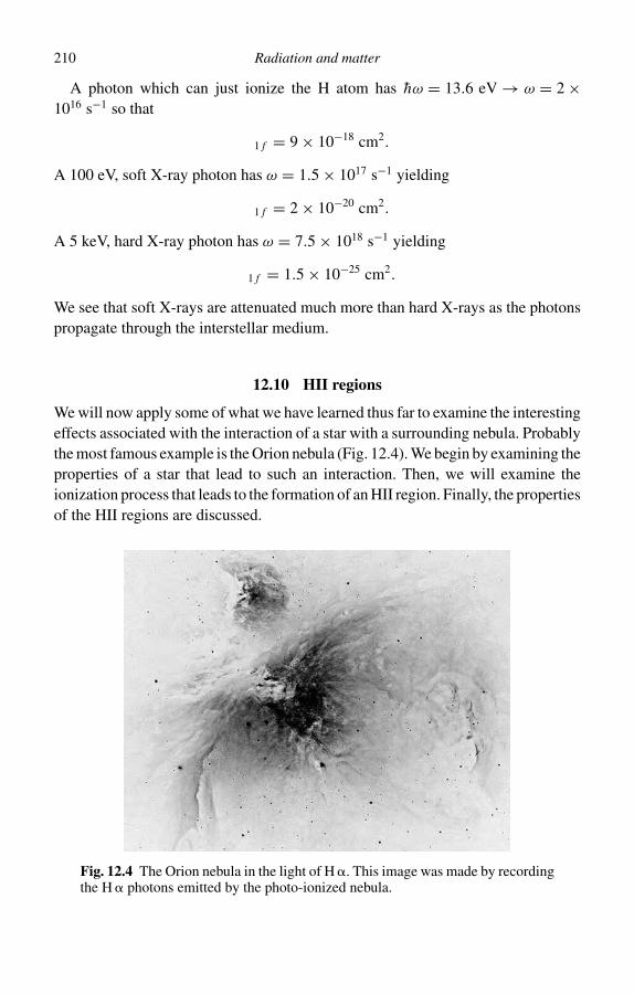
210 Radiation and matter
A photon which can just ionize the H atom has hω = 13.6 eV → ω = 2 ×10¹⁶ s−1 so that
σ1 f = 9 × 10⁻¹⁸ cm2.
A 100 eV, soft X-ray photon has ω = 1.5 × 10¹⁷ s−1 yielding
σ1 f = 2 × 10⁻²⁰ cm2.
A 5 keV, hard X-ray photon has ω = 7.5 × 10¹⁸ s−1 yielding
σ1 f = 1.5 × 10⁻²⁵ cm2.
We see that soft X-rays are attenuated much more than hard X-rays as the photonspropagate through the interstellar medium.
12.10 HII regions
We will now apply some of what we have learned thus far to examine the interestingeffects associated with the interaction of a star with a surrounding nebula. Probablythe most famous example is the Orion nebula (Fig. 12.4). We begin by examining theproperties of a star that lead to such an interaction. Then, we will examine theionization process that leads to the formation of an HII region. Finally, the propertiesof the HII regions are discussed.
Fig. 12.4 The Orion nebula in the light of H . This image was made by recordingthe H photons emitted by the photo-ionized nebula.

12.10 HII regions 211
dA n
dW k
Fig. 12.5 The geometry that defines the intensity,
12.10.1 Ionizing stars
Stars with photospheric temperatures in excess of 104 K emit a significant numberof photons whose energies are greater than 13.6 eV, the ionization potential ofhydrogen. Consequently, if such a star is immersed in a cloud of neutral hydrogen,some of that cloud will be ionized, leading to the formation of an HII region, thatis, a region of ionized hydrogen.
The spectrum of a star, to a good approximation, is that of a black body whosetemperature is that of the star’s photosphere. The spectrum can therefore be de-scribed with the Planck law
Iν = 2hν3/c2
ehν/kT + 1erg cm−2 s−1 Hz−1 sr−1
where ν is the frequency of the emitted radiation and T is the temperature of thephotosphere. The intensity, Iν is defined by
dE = Iν k · n dA dΩ dν dt
where k is the direction of the emitted radiation and n is the direction of the normalof the surface from which the radiation is emitted (see Fig. 12.5).
In order for a star to ionize HI, it must produce reasonable quantities of Lymancontinuum photons (photons with hν > 13.6 eV or ν > ν0 = 3 × 10¹⁵ Hz). In termsof photons, the Planck curve can be rewritten as
Nε = 1.6 × 10²² 2ε2
eε/kT + 1cm−2 s−1 eV−1 sr−1 (361)
where ε is the energy of the photon in electronvolts. Thus the number of photonsemitted with ε > 13.6 eV is given by
Ni = 1.6 × 10²²∫ ∞
13.6 eV
2ε2
eε/kT + 1dε cm−2 s−1 sr−1.

212 Radiation and matter
The fraction of a star’s emitted photons that can ionize HI is therefore given by
fi =∫ ∞
hν0
2ε2
eε/kT + 1
/∫ ∞
0
2ε2
eε/kT + 1= Ni/N .
For the Sun, which has a photospheric temperature of 5600 K, the fraction is4 × 10−10. For an A0 star with a temperature of 10 000 K, the fraction is 3 × 10⁻⁵.For a B0 star with T = 30 000 K, 12% of the emitted photons are ionizing. In thecase of the hottest stars, the O5 stars, the fraction is more like 45%.
Integration of (361) with respect to dA, dΩ and dε yields the luminosity of thestar in photons per second. For a spherically symmetric star
N = (4)2N R2∗
and
Ni = (4)2Ni R2∗ = 1046 fi (R∗/R)2 s−1
where R∗ is the radius of the star.
12.11 Ionization of a pure hydrogen nebula
The ionizing radiation of the star interacts with the surrounding HI atoms. Thenumber of such photons incident on the atoms per unit area per unit time is obtainedby integrating (361) with respect to the solid angle, dΩ . The ionization rate per unitvolume is then given by the product of the atom number density, the ionization rateand the cross-section for bound–free absorption
1.6 × 10224 nH
∫ ∞
13.6 eV
2ε2 σb f (ε)
eε/kT + 1dε cm−3 s−1.
The cross-section can be approximated by recognizing that almost all of the Hatoms are in the ground state when neutral. One way to see that is to consider thespontaneous transition probabilities for hydrogen. Some of the various transitionsare shown in Fig. 12.6.
The transition rate between any two levels can be approximated by the formula
Ann′ ≈ 1.6 × 10¹⁰[n3n′(n2 − n′2)]−1.
Some examples
A2,1 = 5 × 10⁸ s−1
A5,4 = 3.6 × 10⁶ s−1
A10,9 = 9.3 × 10⁴ s−1
A110,109 = 0.5 s−1.

12.11 Ionization of a pure hydrogen nebula 213
1s
2s 2p
3s 3p 3d
4s 4p 4d 4f
Fig. 12.6 The energy level diagram for hydrogen. Energy levels to n = 4 areshown. The dashed lines indicate all permitted transitions to n = 3 and lower.
We see that there is a strong tendency for the electron to descend into the groundstate. Thus, the approximation that all electrons are in the ground level is a reason-able one. We therefore make the approximation that σb f (ν) = σ1 f (ν) = σν so that(360) can be used. The electrons freed by the ionizations will recombine at a rategiven by
n pneαA
where αA ∝ veσ f b is the recombination coefficient and has units cm3 s−1. It isdefined by
αA =∑n,l
αnl
and
αn,l =∫ ∞
0vσnl f (v) dv
where
f (v) = 4√
( m
2kT
)3/2v2 e−mv2/2kT .
See tabulated values of α in Table 12.1.
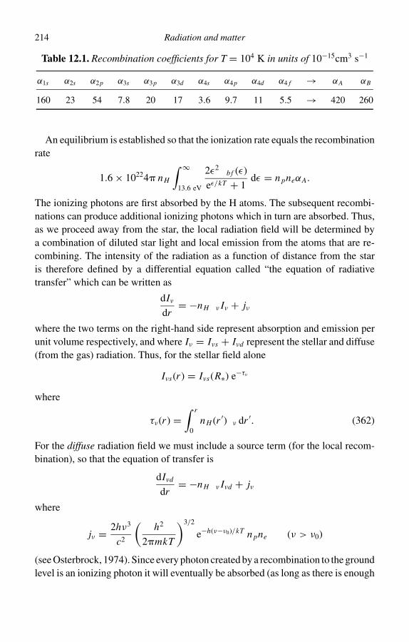
214 Radiation and matter
Table 12.1. Recombination coefficients for T = 104 K in units of 10−15cm3 s−1
α1s α2s α2p α3s α3p α3d α4s α4p α4d α4 f → αA αB
160 23 54 7.8 20 17 3.6 9.7 11 5.5 → 420 260
An equilibrium is established so that the ionization rate equals the recombinationrate
1.6 × 10224 nH
∫ ∞
13.6 eV
2ε2 σb f (ε)
eε/kT + 1dε = n pneαA.
The ionizing photons are first absorbed by the H atoms. The subsequent recombi-nations can produce additional ionizing photons which in turn are absorbed. Thus,as we proceed away from the star, the local radiation field will be determined bya combination of diluted star light and local emission from the atoms that are re-combining. The intensity of the radiation as a function of distance from the staris therefore defined by a differential equation called “the equation of radiativetransfer” which can be written as
dIνdr
= −nHσν Iν + jν
where the two terms on the right-hand side represent absorption and emission perunit volume respectively, and where Iν = Iνs + Iνd represent the stellar and diffuse(from the gas) radiation. Thus, for the stellar field alone
Iνs(r ) = Iνs(R∗) e−τν
where
τν(r ) =∫ r
0nH (r ′)σν dr ′. (362)
For the diffuse radiation field we must include a source term (for the local recom-bination), so that the equation of transfer is
dIνd
dr= −nHσν Iνd + jν
where
jν = 2hν3
c2
(h2
2mkT
)3/2
e−h(ν−ν0)/kT n pne (ν > ν0)
(see Osterbrock, 1974). Since every photon created by a recombination to the groundlevel is an ionizing photon it will eventually be absorbed (as long as there is enough

12.11 Ionization of a pure hydrogen nebula 215
100
0.2
0.4
0.6
0.8
1.0F
ract
iona
l ion
izat
ion
T = 4.0 x 10⁴ K*Black body
Distance, r (pc)2 4 6 8
Fig. 12.7 Fractional ionization as a function of distance from the center of an HIIregion. Note the sharp fall-off that defines the edge of the HII region.
gas around). Thus, any such photons must be local in origin so that dIνd/dr = 0and
Iνd = jνnHσν
and
4
∫ ∞
ν0
jνhν
dν = n pneα1.
Thus, for any point in the nebula
4nH
∫ ∞
ν0
Iνhν
σν e−τν (r ) dν + n pneα1 = n pneαA.
But αA = αB + α1, so we finally have
4nH
∫ ∞
ν0
Iνhν
σν e−τν (r ) dν = n pneαB . (363)
Equations (362) and (363) can be used to solve for nH (r ) and ne(r ) given an input gasdensity distribution, n(r ) = nH (r ) + ne(r ). A typical solution is shown in Fig. 12.7.

216 Radiation and matter
Note that the HII region has a very sharp boundary. The gas is fully ionized insidethe boundary and fully neutral outside.
12.11.1 Radius of HII region
Equations (362) and (363) can also be combined to solve for the radius of the HIIregion. Taking the differential form of (362)
dτν
dr= nHσν.
Combining with (363) yields
4
∫ ∞
ν0
Iνhν
dνdτ
dre−τν (r ) = n pneαB .
Integrating over all space and assuming spherical symmetry
4
∫ ∞
ν0
Iνhν
dν
∫ ∞
0d (−e−τν )4r2 dr =
∫ r0
0n pneαB4r2 dr.
On the right-hand side we have recognized that there is no ionized gas outside r0.Evaluating these integrals and rearranging terms, we have∫ ∞
ν0
(4)2r2 Iν/hν dν = 4
3r3
0 n pneαB .
But Lν = (4)2r2 Iν , so that∫ ∞
ν0
Lν/hν dν = Ni = 4
3n pneαBr3
0 .
Solving this for r0
r0 =[
3Ni
4n2eαB
]1/3
= 104 N 1/3i
( ne
1 cm−3
)−2/3. (364)
The quantity r0 is often referred to as the Stromgren radius and the quantity(4/3) r3
0 as the Stromgren sphere.According to (364), Ni can be calculated for any star. Table 12.2 lists the size of
the Stromgren sphere predicted for four different types of star.
12.12 Quasars and the Lyman forest
Quasars are compact, stellar-like objects when imaged on photographic plates orby CCD cameras. What makes them unique is their often tremendous redshifts.Figure 12.8 shows the spectra of four distant quasars.

12.12 Quasars and the Lyman forest 217
Table 12.2. Stromgren spheres. The table shows the size of theionizing star in solar radii, the log of the ionization rate and the
size of the corresponding Hll region in parsecs. An ambientdensity of one particle per cubic centimeter is assumed.
Spectral type R/R log Ni r0 (pc)
O5 10 50.0 142B0 7.0 48.7 50A0 2.5 42.7 0.6G2 1.0 36.3 5 × 10⁻³
Fig. 12.8 Spectra of four quasars with z > 4. The spectral lines are annotated.Note the observed wavelengths of the Ly- line compared to the rest wavelengthof 1216A. From Schneider, D. P., Schmidt, M. and Gunn, J. E. 1997, AJ, 114, pp.36–40.
The most distant quasars also show complex absorption spectra which contain thesame line observed over a wide range of wavelengths. For example, Fig. 12.9 showsa large number of Lyman lines spaced out over a wide range of wavelengths. It isdoubtful that a single source could account for the range in velocity (and thereforedistance). It has therefore been proposed that the absorption line system (the forest)is caused by intervening galaxies or clouds of gas. The intervening objects, although

218 Radiation and matter
250200150100500
3400 3600 3800
4000 4200 4400 46000
200400600800
1000
1000
500
0
4600 4800 5000 5200 56005400
KP 76
Fig. 12.9 Lyman forest. The observations are taken from Crotts, A. P. S. andFang, Y. (1998, ApJ, 502, pp. 16–47).
closer than the quasar in question, are probably also in their earlier phases ofevolution. The distribution of these objects in velocity space provides an importantclue on the distribution of matter in the distant Universe. This is particularly truegiven that the matter sampled in the Lyman forest is fairly old, that is the Lyman photons left the scene billions of years ago. Did the Universe at that time havesimilar structure to the modern Universe?
12.12.1 Correlation studies
Features in the Lyman forest are separated in velocity space by amounts rangingfrom the instrumental spectral resolution to the entire range in velocities observed.The question is whether the distribution of possible values of v is different froma random distribution.

12.12 Quasars and the Lyman forest 219
8
6
4
2
0
0 500 1000 15000∆v (km s−1)
Num
ber
of p
airs
Fig. 12.10 Correlation statistics for a Lyman forest. The figure is taken fromCrotts, A. P. S. and Fang, Y. (1998, ApJ, 502, pp. 16–47).
Let
v = c[(
λλ0
)1 − (
λλ0
)2
]1 + ⟨
λλ0
⟩where the subscripts 1 and 2 refer to any pair of Lyman lines. We can then definea two-point correlation function, ζ , such that
ζ (v) = Nobs(v)
Np(v)− 1
where Nobs(v) is the number of observed pairs at a given v and Np(v) is thenumber expected from a purely random distribution.
Figure 12.10 is taken from Crotts and Fang (1998) and shows a correlation plot.Note that the excursions from ζ = 0 are not significant, suggesting that there is nostrong clustering of Lyman lines in the forest. Such results suggest that if thelines arise from intervening galaxies, the galaxies are not as strongly clustered as

220 Radiation and matter
they have become. Some astronomers have taken this to mean that the interveningmatter is not galaxies at all but rather a general intergalactic medium in the form ofclouds. The issue is not yet totally settled. If there is an intergalactic medium it isfairly tenuous as the following estimate shows.
12.12.2 Column density of the HI responsible for the Ly − forest
Using our definition of optical depth we write down the opacity arising from onecloud as
τ = n1σ12r = dN1σ12
where n1 represents the number density of hydrogen atoms in the ground state, σ12 =3 × 10⁻¹¹ cm2 is the Lyman absorption cross-section as defined on page 209 andr is taken to be the dimension of the cloud responsible for a specific Lyman
feature. The column density associated with one cloud is N1.If the clouds are moving as a result of the Hubble flow then we can relate r to
the line spacings in the Ly- forest
dv = H r
where dv is the minimum resolved line spacing in velocity space.The observed absorption lines are unsaturated suggesting that τ < 1 so that
dN1σ12 ≤ 1 → dN1 ≤ 3 × 1010 cm−2.
Summing over the entire Lyman forest
NH =∫ r0
0n1 r =
⟨dN1
r
⟩r0 ≈ 〈dN1〉 v0
dv
where v0 is the recession velocity of the quasar. Using these numbers
NH ≤ 3 × 10¹⁰ 2.7 × 10¹⁰
5 × 10⁶≈ 2 × 1014 cm−2
which is about six orders of magnitude smaller than the column density of HI inour own Galaxy.
12.13 Reference
Crotts, A. P. S. and Fang, Y. (1998) Re-observation of Close QSO Groups: The SizeEvolution and Shape of Ly alpha Forest Absorbers, The Astrophysical Journal, 502,pp. 16–47.

12.14 Further reading 221
12.14 Further reading
Cohen-Tanoudji, C. (1992) Principles of Quantum Mechanics, John Wiley and Sons, NewYork, NY, USA.
Griffiths, D. (1995) Introduction to Quantum Mechanics, Prentice Hall, Englewood Cliffs,NJ, USA.
Landau, L. D. and Lifschitz, E. M. (1977) Quantum Mechanics, 3rd edn, Pergamon Press,Oxford, UK.
Landau, R. H. (1996) Quantum Mechanics II: A Second Course in Quantum Theory, 2ndedn, John Wiley and Sons, New York, NY, USA.
Osterbrock, D. E. (1974) Astrophysics of Gaseous Nebulae, W. H. Freeman, SanFrancisco, CA, USA.
Rybicki, G. B. and Lightman, A. P. (1985) Radiative Processes in Astrophysics, JohnWiley and Sons, New York, NY, USA.
Shu, F. H. (1992) The Physics of Astrophysics: Radiation, University Science Books, MillValley, CA, USA.

Chapter 13
Atomic fine structure lines
13.1 Electron spin
Some of the most important astrophysical transitions involve electron spin. Perhapsthe most famous example is the 21 cm line. We will now consider the role of electronspin in atomic transitions. The non-relativistic Hamiltonian, introduced earlier, con-tains no spin-specific terms (it allows only for orbital angular momentum throughthe operator L). As I will now demonstrate, the relativistic Hamiltonian providesadditional degrees of freedom so that effects like spin (nuclear and electron) canbe incorporated into the Schrodinger equation. To that end we now discuss Dirac’spostulate, spin angular momentum, Dirac’s equation, the non-relativistic limit, rel-ativistic corrections, transitions involving spin, the Zeeman effect and spin–orbitcoupling. Discussion of these topics will give us an understanding of atomic finestructure.
13.1.1 Relativistic Hamiltonian
Recall the form of the relativistic Hamiltonian (see, for example, Shu, 1992).
H = [|c P|2 + m2c4]1/2 + qΦ (365)
where
P = p − q
cA.
It is difficult to use the above as an operator because it is nonlinear. Let us thereforesquare the operators of
HΨ = i h∂Ψ
∂t→ H 2Ψ = −h
∂2
∂t2Ψ.
222

13.2 Dirac’s postulate 223
With no scalar potential the above reduces to[(|c P|2 + m2c4) − h2 ∂2
∂t2
]Ψ = 0.
With no vector potential we get the Klein–Gordon (K–G) equation[(∇2 − 1
c2
∂2
∂t2
)−
(mc
h
)2]
Ψ = 0. (366)
Note that Ψ is not a wave function. It is a scalar field which must be describedusing Quantum Field theory.
13.2 Dirac’s postulate
To circumvent the problem with the K–G equation, Dirac proposed a Hamiltonianof the form
H = a · Pa + bmc2 + qφ (367)
where a and b are constants.To make (367) equivalent to (365) requires
axax = ayay = azaz = bb = 1
axay + ayax = ayaz + azay = azax + axaz
= ax b + bax = ayb + bay = azb + baz = 0.
This can only hold if ax , ay , az and b form 4 × 4 matrices. Thus
ax =(© σx
σx ©)
and ay =(© σy
σy ©)
az =(© σz
σz ©)
and b =(
I ©© −I
) (368)
where
© ≡(© ©
© ©)
and I ≡(
1 ©© 1
)
and the Pauli matrices are
σx =(© 1
1 ©)
and σy =(© −i
i ©)
and σz =(
1 ©© −1
). (369)

224 Atomic fine structure lines
See Shu (pp. 268–9 in that book) for suggestions on proof. The properties of thePauli matrices can be summarized as
σiσk − σkσi = 2iεikmσm(370)
σiσk + σkσi = 2ik .
Rotation and angular momentum
We can write (370) in operator form, so that
σ × σ = 2i σ .
Note the analogy to
L × L = i h L⇒ let s = h
2σ ⇒ s × s = i hs.
13.2.1 The Dirac equation
The Dirac equation gives us a mathematical feel for the extra degrees of freedomthat allow us to include spin in the definition of the wave function, Ψ .
To make use of (367) we need a four-component Ψ because the operators are4 × 4 matrices,
Ψ ⇒ χ ≡
χ1
χ2
χ3
χ4
so that
⇒[ca ·
(i h ∇ + e
cA)
+ bmec2]χ =
(i h
∂
∂t+ eφ
)χ. (371)
It follows that the probability density is given by
g = χ †χ = |χ1|2 + |χ2|2 + |χ3|2 + |χ4|2
where † = Hermitian complex conjugate.
13.2.2 Free particle at rest
Normally, the Dirac equation is too complicated to be solved analytically. However,there exists a simple but important application of the Dirac equation. It will serveto illustrate how the Dirac equation is used in practice.

13.2 Dirac’s postulate 225
For a free particle, φ, A = 0, so that the Dirac equation becomes
⇒ [−i hca · ∇ + bmec2]χ = i h∂χ
∂t. (372)
Let us try a solution of the form
χ = χ0(ke) ei(ke·x−Et/h). (373)
Given that ke = 0, substitute (373) into (372) to yield
mec2
(I ©© I
) (Ψ+Ψ−
)= E
(Ψ+Ψ−
)
where
χ0 =(
Ψ+Ψ−
)2 × 2-component spinors
spinor:Ψ+ = ψ+
+α+ + ψ+−α−
Ψ− = ψ−+α+ + ψ−
−α−
α+ =
(1
0
), α− =
(0
1
).
Thus
mec2Ψ+ = EΨ+ ⇒ E = mec2
−mec2Ψ− = EΨ− ⇒ E = −mec2
E = 2mec2.
The negative rest mass energy led Dirac to propose the existence of the positron. Theenergy difference is the difference in rest mass energies of electrons and positrons.
13.2.3 Non-relativistic limit of Dirac’s equation
By examining the behavior of the Dirac equation in the non-relativistic limit wecan simplify the Hamiltonian but retain the effects of spin. Let
E ≡ i h∂
∂t− mec2 (374)
P ≡ −i h ∇ + e
cA. (375)
Consider the limit of (371) when E and P are small compared to mec2 and mecrespectively.
Let us define wave function χ such that
χ =(
Ψ+Ψ−
)(376)

226 Atomic fine structure lines
so that (371) becomes
(E + eφ)Ψ+ − cσ · PΨ− = 0 (377)
(E + 2mec2 + eφ)Ψ− − cσ · PΨ+ = 0 (378)
where
σ ≡ σx x + σy y + σz z.
Equation (378) can be written as
Ψ− = [2mec2 + (E + eφ)]−1cσ · PΨ+. (379)
For E + eφ 2mec2
⇒ [2mec2 + (E + eφ)]−1 ≈ 1
2mec2
(1 − E + eφ
2mec2
).
Substituting this into (377)
⇒[
(E + eφ) − σ · P2me
(1 − E + eφ
2mec2
)σ · P
]Ψ+ = 0 (380)
correct to order v2/c2!To simplify further we factor out the dependence on rest energy so that
EΨ+ = E(Ψ (x, t) e−imec2t/h) = i h∂Ψ
∂te−imec2t/h.
Substituting into (380) with the definition of E and after a little manipulation allthe mec2 terms cancel out so that
⇒ SΨ = 0 S = S0 + S2 (381)
where
S0 =(
i h∂
∂t+ eφ
)− (σ · P)2
2me
and
S2 = σ · P2mec
(i h
∂
∂t+ eφ
) σ · P2mec
.
In the fully non-relativistic limit S0 S2 so that
⇒ S0Ψ = 0. (382)

13.3 Radiative transitions involving spin 227
Since σ operates in a different space than P(σ · P)2 = P · σ σ · P (383)
⇒ σiσk = 1
2[(σiσk + σkσi ) + (σiσk − σkσi )]
= ik + iεikmσm
which implies
P · σ σ · P = | P|2 + i σ · ( P × P) (384)
where
P = −i h ∇ + e Ac
⇒ P × P = 0.
We are now in the position of working out two do-able cases.Case A: Discard terms of ≈ v2/c2. Radiative transitions involving spin.Case B: Consider terms of ≈ v2/c2 but let A = 0.
The former allows us to describe radiative transitions involving spin (Section13.3), the latter describes spin–orbit coupling (Section 13.4).
13.3 Radiative transitions involving spin
Recall
P = p + e Ac
= −i h ∇ + e Ac
A = 0
so that (384) becomes
P · σ σ · P =∣∣∣ p + e
cA∣∣∣2
+ eh
cσ · ( ∇ × A). (385)
So take (381) for S0 and put it into Hamiltonian form
⇒ S0Ψ = 0 ⇒ (H0 + H1 + H2 + HBS) Ψ = i h∂Ψ
∂t(386)
where, as before
H0 + H1 + H2 = 1
2me
∣∣∣p + e
cA∣∣∣2
− eφ
and HBS contains the spin term in (385)
HBS = eh
2mecσ · ( ∇ × A) = eh
2mec
(2
hs)
· B
⇒ HBS = e
mecs · B. (387)

228 Atomic fine structure lines
As we noted earlier, s acts as a spin-angular-momentum operator, so that(s2
x + s2y + s2
z
)α± = 3
4 h2α ±szα± = ± 1
2 hα ±(sx ± isy)α∓ = hα ±(sx ± isy)α± = 0.
Define ± 12 terms with ms = 1
2 (spin up), = − 12 (spin down). Now suppose
A = Arad + 1
2B0 × x . (388)
The modified potential still satisfies the Coulomb gauge but ∇ × A → static field
⇒ HBS = H radBS + Hzs
H radBS = (e/mec)s · ( ∇ × Arad) (389)
HzS = (e/mec)s · B0.
The H radBS does not contribute to the transition matrix element in the same multipole
order as the largest term present in H . Note the parallel between k × eα and ∇ ×Arad = Brad. We see that magnetic dipoles interact only with the B part of the EM
field.
13.3.1 Zeeman effect
The previous discussion allows us to describe the Zeeman effect. We begin byexamining the static B0 portion of H1, and express the Hamiltonian as
HzL = e
2mec( B0 × x) · p = e
2mecB0 · L.
Then, we add HzS to get the total Hz ,
Hz = −eB0
2mec· (L + s) = − B0 · ( M + m). (390)
The Zeeman effect is an example of spin coupling.
13.4 Relativistic correction with A = 0
Letting A = 0 reduces P to the canonical momentum, p, so that
P = p ⇒ p · σ σ · p = | p|2.

13.5 Atomic fine structure 229
Retaining the relativistic corrections to v2/c2 yields
S = S0 + S2 → S ′ = S0 + 1/(8m2
ec2)eh(∇2φ) + | p|4/me
+ 2eh σ · [( ∇φ) × (p)]⇒solve S ′Ψ ′ = 0.
(391)
In Hamiltonian form S ′ = H − i h(∂/∂t), so if we compare with (391)
⇒ HS = S0 − i h∂
∂t= i h
∂
∂t+ eφ − | p|2
2me− i h
∂
∂t
we get
⇒ HS = | p|22me
− eφ (392)
the structure Hamiltonian
Hk = | p|48m2
ec2(393)
the relativistic correction for kinetic energy
H0 = −eh2
8m2ec2
∇2φ (394)
the relativistic correction for the potential, affecting only the = 0 term and
HSO = −es · [( ∇φ) × p]
2mec2(395)
the term representing spin–orbit coupling where s = (h/2)σ . Note that spin–orbitcoupling is like a self induced Zeeman splitting because it is the motion of theelectron in the potential that produces a local B field (recall Ampere’s law). Spin–orbit coupling accounts for the fine structure of atoms.
13.5 Atomic fine structure
I now examine the nature of the spin–orbit interaction. In the process, I will solvefor the energy eigenvalues of the spin–orbit Hamiltonian. I conclude by describingthe fine structure of the atomic energy levels of hydrogen.

230 Atomic fine structure lines
13.5.1 Spin–orbit interaction
The total angular momentum is now the sum of spin and orbital angular momenta
J = L + Swhich requires a change of counters: m → m, and addition of ms, j so that thenew eigenket is |n, , j, m, ms〉.
13.5.2 Time-independent perturbation theory
Spin lifts the degeneracy with respect to and m.We want to solve
(H0 + HSO ) Φ = EΦ
where, from (395)
HSO ∝ S · ( ∇φ × p) ∝ S ·(
1
r
dV
drr × p
)∝ 1
r
dV
drS · L
so that
HSO = 1
2m2ec2
(1
r
dV
dr
)S · L. (396)
Let Φ be a linear superposition of unperturbed states
Φ =∑
m ′,m
′s
C(m ′, m ′
s)|n, , m ′, m ′
s〉
where
|n, , m ′, m ′
s〉 = 1
rRn,(r )Y,m ′
α±.
Substituting the above into (396) yields∑m ′
,m′s
(En − E + HSO )|n, , m ′, m ′
s〉C(m ′, m ′
s) = 0.
Left multiply by 〈n, , m, ms |∑m ′
,m′s
(−ESOm,m ′ms ,m ′
s+ 〈n, , m, ms |HSO |n, , m ′
, m ′s〉)C(m ′
, m ′s) = 0
where
ESO ≡ E − E0 = E − En.

13.5 Atomic fine structure 231
Since α± is a two-column matrix we can cast the above as(A++ A+−A−+ A−−
) (C+C−
)= 0. (397)
Each A has (2 + 1)2 matrix elements from the 2 + 1 values of ml in C . Thus
A++ =
H++ − ESO H++
,−1 . . . H++,−
H++−1, H++
−1,−1 − ESO . . . H++−1,−
. . . . . . . . . . . .
H++−, H++
−,−1 . . . H++−,− − ESO
(398)
where
H±±mm ′
≡ 〈n, , m, ±1/2|HSO |n, , m ′
, ±1/2〉 (399)
and
C+ ≡
C(, +1/2)C( − 1, +1/2)
.
.
.
C(−, +1/2)
C− ≡
C(, −1/2)C( − 1, −1/2)
.
.
.
C(−, −1/2)
. (400)
The requirement for solving (397) is∣∣∣∣ A++ A+−A−+ A−−
∣∣∣∣ = 0 (401)
which yields a characteristic equation for ESO as a polynomial of order 2(2 + 1).The roots are eigenvalues corresponding to the perturbation energies.
13.5.3 The jm representation
Substituting (396) into (399) yields
H±±mm ′
=
[1
2m2ec2
∫ ∞
0
1
r
dV
drR2
n(r ) dr
]〈Ym
α(ms)| S · L|Ym ′α(m ′
s)〉 (402)
where
S · L ≡ Sx Lx + Sy L y + Sz Lz.
Note that Sx Lx + Sy L y = 12 [(Sx + i Sy)(Lx − i L y) + (Sx − i Sy)(Lx + i L y)].
These are raising and lowering operators so that
(Lx ± i L y)Ylm = [(l ∓ m)( ± 1 + m)]1/2 hY,m±1

232 Atomic fine structure lines
and
(Sx ± i Sy)α∓ = hα±
so that
〈Y,mα(ms)|Sx Lx + Sy L y|Y,m ′
α(m ′
s)〉 = 0
unless m ′s + m ′
= ms + m, while
〈Y,mα(ms)|Sz Lz|Y,m ′
α(ms)〉 = 0
unless m ′s = ms and m ′
= m, consistent with the above constraint. Thus
H±±mm ′
=
0, m ′
s + m ′ = ms + m
= 0, m ′s + m ′
= ms + m = m
⇒ m = ms + m is a good quantum number.Since J 2Φ = j( j + 1)h2Φ, j is also a good quantum number.Given that J 2 = S2 + L2 + 2 S · L we have
[ j( j + 1)]max = s(s + 1) + ( + 1) + 2s
[ j( j + 1)]min = s(s + 1) + ( + 1) − 2s
so that − s ≤ j ≤ + s in increments of 1!Thus, in the jm representation, the new eigenket becomes |n, , j, m〉.
13.5.4 Solution for ESO
We can now drop the n from the eigenket so that Φ = | jm〉. Substituting into theSchrodinger equation yields
E = 〈 jm|H0| jm〉 + 〈 jm|HSO | jm〉 = E0 + ESO
where
ESO =[
1
2m2ec2
∫ ∞
0
1
r
dV
drR2
n dr
]〈 jm| S · L| jm〉.
But S · L = 1/2[J 2 − L2 − S2] is diagonal in the jm representation
⇒ 〈 jm| S · L| jm〉 = 1
2[ j( j + 1) − ( + 1) − s(s + 1)]h2
=
(/2)h2, j = + 12
−( + 1)h2/2, j = − 12 .

13.5 Atomic fine structure 233
n = 2
n = 3 j = 1/2 j = 1/2
j = 3/2
j = 3/2
j = 5/2
j = 1/2 j = 1/2
j = 3/2
2s2p
1/21/2
Lamb shiftl = 0 l = 1l = 0 l = 1
l = 2
Fig. 13.1 The fine structure associated with the Hα transition. The expandedregion shows the Lamb Shift which is not predicted by Dirac theory.
For a hydrogen atom, V = −e2/r . Substituting into the previous equation andgrouping terms
⇒ ESO = |En| α2
n( + 1
2
)( + 1)
/2, j = + 1
2
−( + 1)/2, j = − 12 .
The corresponding perturbation from the relativistic correction is
Ek = −|En|α2
n2
(n
+ 12
− 3
4
).
Adding ESO and Ek yields
E = Ek + ESO = −|En|α2
n2
(n
j + 12
− 3
4
). (403)
For j = 1/2, 3/2, . . . , n − (1/2).We see that levels are still degenerate with respect to m but not with respect to
j . Applying (403) to the n = 4 level of hydrogen, as an example, we see that there

234 Atomic fine structure lines
are now four levels
E = −|E4|α2
1316 , j = 1
2
564 , j = 3
2
7176 , j = 5
2
164 , j = 7
2 .
Spin–orbit coupling produces fine structure of the order of α2 of the unperturbedenergy. The new dipole selection rules are
m = 0, ±1 = ±1 j = 0, ±1.
The fine structure associated with the Hα transition is shown in Fig. 13.1.
13.6 Further reading
Cohen-Tanoudji, C. (1992) Principles of Quantum Mechanics, John Wiley and Sons,New York, NY, USA.
Dirac, P.A.M. (1982) Principles of Quantum Mechanics, 4th edn, Oxford UniversityPress, Oxford, UK.
Griffiths, D. (1995) Introduction to Quantum Mechanics, Prentice Hall, Englewood Cliffs,NJ, USA.
Landau, L. D. and Lifschitz, E. M. (1977) Quantum Mechanics, 3rd edn, Pergamon Press,Oxford, UK.
Landau, R. H. (1996) Quantum Mechanics II: A Second Course in Quantum Theory, 2ndedn, John Wiley and Sons, New York, NY, USA.
Osterbrock, D. E. (1974) Astrophysics of Gaseous Nebulae, W. H. Freeman, SanFrancisco, CA, USA.
Shu, F. H. (1992) The Physics of Astrophysics: Radiation, University Science Books, MillValley, CA, USA.

Chapter 14
Atomic hyperfine lines
In expanding the relativistic Hamiltonian we noted two do-able cases. In the firstcase, we demonstrated that interactions of spin and orbital momentum with mag-netic fields can take place thereby producing fine structure. In the second case, weshowed that an electron’s spin can interact with its orbital momentum (self inducedZeeman effect) to produce atomic fine structure. Of special interest in Case A is thespin–spin interaction. In that case the electron’s spin interacts with the magneticfield produced by the spin of the nucleus. The spin–spin interaction is therefore anexample of the Zeeman effect which leads to hyperfine structure. We now proceedto examine the spin–spin interaction in the ground state (1S1/2) of hydrogen. Notethat spin–orbit coupling alone does not split this state.
14.1 The 21 cm line of hydrogen
The spin magnetic moments of the electron and nucleus are given by
m = − gee
2mecs (404)
M = gpe
2m pcS (405)
respectively, where ge and gp are the so-called g factors of the electron and nucleus.Associated with M is a magnetic field. Recall that for a dipole field
B = 3( M · k)k − M|x |3 (406)
where k represents the direction of the dipole moment and x is the distance fromthe center of the dipole.
235

236 Atomic hyperfine lines
F = 1n = 1
n = 1 F = 0
E = h νFig. 14.1 Hyperfine splitting of the ground state of hydrogen. Transitions betweenthe F = 1 and F = 0 states lead to the 21 cm line. Shown are the relative alignmentsof the proton and electron spins.
According to our earlier discussions we can calculate the Zeeman effect
Hm = HzS = e
mecs · B = − m · B. (407)
Since the proton (nucleus) and electron each have a spin of 1/2 there are fourpossible combinations for the combined wave function. We define a total spin Fsuch that F = S + s. Therefore there are three possible states that produce F = 1and one state that produces F = 0 (Fig. 14.1)
Σ F2
Fz= Σ1
±1, Σ10 , Σ0
0 (408)
where
Σ1±1 = α±(p)α±(e)
Σ10 = 1√
2[α+(p)α−(e) + α−(p)α+(e)] (409)
Σ00 = 1√
2[α+(p)α−(e) − α−(p)α+(e)].
The energies of the levels can be calculated in the usual way by taking the expec-tation value of the Hamiltonian
Em = 〈φΣ |Hm |φΣ〉 (410)
where φ is the unperturbed wave function for the ground state of hydrogen and isgiven by
φ = 2r−3/20 e−r/r0Y00 (411)
while Σ corresponds to the four spin states previously described.

14.1 The 21 cm line of hydrogen 237
Direct substitution of equations (404) and (411) into (410) results in a divergentintegral. We therefore have to resort to a trick first formulated by Fermi.
Fermi’s trick
We know that for a magnetic dipole (see Jackson, 1998)
A = ∇ ×( M
r
)(412)
so that the B field can be written as
B = ∇ × A → ∇ ×[
M × ∇(
1
r
)]. (413)
From (407), Hm = − m · B. Inserting (413) yields
Hm = ( m · M)∇2
(1
r
)− [( m · ∇)( M · ∇)]
1
r.
Subtracting one-third of the first term from the first term and adding this to thesecond term yields
Hm = H (0)m + H (2)
m
where
H (0)m = 2
3( m · M)∇2
(1
r
)(414)
and
H (2)m = −[( m · ∇)( M · ∇) − 1/3( m · M)∇2]
1
r.
We see that the bad behavior at r = 0 is localized to H (2)m . However, when inserted
into (410) it yields only spherical harmonics, but because it is operating on aspherically symmetric function (411) the net result from the operation is 0. Thus⟨
φΣ∣∣H (2)
m
∣∣φΣ⟩ = 0
and takes away the bad behavior at r = 0. Thus the remaining expression is
Em = ⟨φΣ
∣∣H (0)m
∣∣φΣ⟩.
Using ∇2(1/r ) = −4(x) with (404) and (414), this reduces to
Em = 2gegpe2
3mem pc2a30
〈Σ |S · s|Σ〉 = 2
3
E0
h2〈Σ |S · s|Σ〉. (415)

238 Atomic hyperfine lines
Now, S · s = 12 ( F · F − S · S − s · s) so that
〈Σ | S · s|Σ〉 = 1
2[〈Σ | F · F |Σ〉 − 〈Σ | S · S|Σ〉 − 〈Σ |s · s|Σ〉]
= 1
2[F(F + 1)h2 − S(S + 1)h2 − s(s + 1)h2].
For F = 1, Em1 = (1/6)E0 and for F = 0, Em2 = −(1/2)E0, where E0 can berewritten as
E0 = gegpα4
(me
m p
)mec2.
The net energy difference between the F = 1 and F = 0 states is given by
E = Em1 − Em2 = 2
3E0 = 6 × 10⁻⁶eV.
For hν = E → ν = 1.420 405 752 × 109 Hz → λ ≈ 21 cm.
14.1.1 Transition rate
Recall that it is the total angular momentum that contributes to the Zeeman effect.In this case the total momentum is S + s. Thus, in analogy to the electric dipoletransition, we can define a magnetic dipole transition as
Ai f = 4ω3
3hc3|〈 f | M + m|i〉|2 (416)
which we get by setting ex → M + m. Now recall that the spin can be expressedin terms of the Pauli spin matrices. Thus
M = µp σ p and m = −µe σe
where
µp = gpeh
4m pcand µe = − geeh
4mec.
For the F = 1 → 0 transition
A10 = 4ω3
3hc3
∣∣⟨Σ00 |µp σp − µe σe|Σ1
⟩∣∣2. (417)
Recall that σ = σx x + σy y + σz z, where σzα± = ±α± and σxα± = α±, σyα± =±iα∓ so that ∣∣⟨Σ0
0 |µp σp − µe σe|Σ1±1
⟩∣∣ = − 1√2
(x ± i y)(µp + µe)
∣∣⟨Σ00 |µp σp − µe σe|Σ1
0
⟩∣∣ = z(µp + µe).

14.1 The 21 cm line of hydrogen 239
Table 14.1. Transitions involving hyperfine structure
Atom Spin Transition Frequency (Hz) A (s−1)
HI 1/2 2S1/2, F = 0 − 1 1.420405751 × 10⁹ 2.85 × 10⁻¹⁵
D 1 2S1/2, F = 1/2 − 3/2 3.27384349 × 10⁸ 4.64 × 10⁻¹⁷
HeII 1/2 2S1/2, F = 1 − 0 8.66566 × 10⁹ 6.50 × 10⁻¹³
NVII 1 2S1/2, F = 1/2 − 3/2 5.306 × 10⁷ 1.49 × 10⁻¹⁹
NI 1 4S3/2, F = 3/2 − 5/2 2.612 × 10⁷ 1.78 × 10⁻²⁰
F = 1/2 − 3/2 1.567 × 10⁷ 3.84 × 10⁻²¹
H+2 1 F2, F = 3/2, 5/2 − 1/2, 3/2 1.40430 × 10⁹ 2.75 × 10⁻¹⁵
F2, F = 3/2, 3/2 − 1/2, 3/2 1.41224 × 10⁹ 2.80 × 10⁻¹⁵
NaI 3/2 2S3/2, F = 1 − 2 1.77161 × 10⁹ 5.56 × 10⁻¹⁵
Recalling that the transition rate is independent of the upper level state we choose(when states are degenerate), we have
A10 = 4ω3
3hc3
∣∣⟨Σ00 |µp σp − µe σe|Σ1
⟩∣∣2 = 4ω3
3hc3(µp + µe)2. (418)
But µe µp so that
A10 = ge
12
(1 + gpme
gem p
)2 (reω
c
) (hω
mec2
)ω (419)
⇒ A10 ≈ 3 × 10⁻¹⁵s−1.
The lifetime of the excited state is ≈ 107 years.Note that the hyperfine structure scales as α4 while the fine structure scales
as α2. The 21 cm line represents the most famous astrophysical transition arisingfrom hyperfine structure. Other hyperfine transitions are also possible and these aresummarized in Table 14.1.
In direct analogy to (384) for the fine structure, the general formula for calculatingenergy hyperfine splitting is given by
ESS = gN (mem p)α2hcRZ3
n3
[F(F + 1) − S(S + 1) − j( j + 1)
j( j + 1)(2 j + 1)
]. (420)
14.1.2 The 21 cm line profile
The natural width of the 21 cm line is Γ ≈ A10 = 3 × 10⁻¹⁵ s−1. The extremelynarrow width follows from the uncertainty principle because of the extremely longlifetime of the excited state. The lifetime is ≈ A−1
10 = 107 years. The naturallynarrow width of this line makes it an ideal diagnostic of interstellar hydrogenbecause the strength of the line depends on the density and temperature of the

240 Atomic hyperfine lines
∗
v x ′
θ ′
^
Fig. 14.2 The geometry associated with the Doppler effect.
hydrogen gas. The latter broadens the line because of differential Doppler shiftsfrom randomly moving hydrogen atoms. In the next section we review the Dopplereffect and then apply it to determine the profile of the 21 cm line.
14.2 The Doppler effect
Consider the motion of an observer relative to a star, as shown in Fig. 14.2. Recallfrom special relativity that energy, E , and momentum, p, make up a four-vector.The E is the fourth component of such a four-vector and therefore transforms as
E = γ (V )[E ′ + V p′x ]
in analogy to
t = γ (V )
[t ′ + V
c2x ′
]
where the primed coordinates refer to the frame of the star. Thus
⇒ E = γ (V )
[E ′ + E ′
cV||
]
where the radial velocity with respect to the star is defined as
V|| = V cos θ ′
so that
E = γ (V )E ′[
1 + V
ccos θ ′
].
For photons we can let E = hν, E ′ = hν ′
ν = ν ′γ (V )[1 + β cos θ ′].

14.2 The Doppler effect 241
All that remains is to transform θ ′ → θ , which we can do by using the aberrationformulae, so that
= ν ′γ[
1 + β
(cos θ − β
1 − β cos θ
)].
Now, let us consider some special cases
θ = 0 : ν = ν ′γ (1 + β) = ν ′ [(1 + β)/(1 − β)]1/2
θ = /2 : ν = ν ′γ (1 − β2) = ν ′[1 − β2]1/2.
We see that at relativistic velocities there is a significant transverse Doppler shiftin addition to the regular radial shift. The transverse shift is always a redshift. Inthe non-relativistic limit, β 1
ν = ν ′
1 + β, θ = 0
1 − 12β
2, θ = /2.(421)
Thus, to first order in β there is only a radial Doppler shift.
14.2.1 Doppler broadening of the 21 cm line
The 21 cm line emissivity of HI gas is given by
jν = hν
4n1 A10φν
where n1 is the number density of HI in the F = 1 state and φν is the normalizedline profile such that ∫ ∞
0φν dν = 1.
Since HI atoms are in collisional equilibrium with each other they follow aMaxwell–Boltzmann velocity distribution. The probability, therefore, of an atom’sradial velocity being between v and v + dv at a temperature T is given by
4 f (v)v2 dv = 4( m H
2kT
)1/2e−(m H v2)/(2kT )v2 dv (422)
where
4
∫ ∞
0f (v)v2 dv = 1.
At interstellar temperatures the HI gas is not relativistic so that (421) can be usedfor the Doppler shift, in which case
ν
ν0= v
c.

242 Atomic hyperfine lines
Combining with (422)
f (ν) =( m H
2kT
)3/2e−(m H c2ν2)/(2kT ν2
0 ). (423)
Similarly
4v2 dv → 4
[νc2
ν20
]c
ν0dν = 4
[2kT
m H
]c
ν0dν.
Combining the last two equations, and insuring normalization, finally yields
φν =[
m H c2
2kT ν20
]1/2
e−(m H c2(ν−ν0)2)/(2kT ν20 t). (424)
This is a Gaussian whose 1/e halfwidth is given by
σν =√
2kT
m H
ν0
c. (425)
For T = 100 K, σν = 7 kHz for the 21 cm line.
14.3 Neutral hydrogen in galaxies
Observations of 21 cm emission can be used to probe neutral hydrogen in galaxies.I begin with a discussion of the equation of transfer for HI emission and its usein determining gas distributions in galaxies. The shape of the 21 cm line providesimportant information on the dynamics of the detected gas. We will therefore discusshow gas dynamics are measured. In the process, we will highlight the problem ofmissing mass and dark matter.
14.3.1 Equation of transfer for HI emission
Earlier, we introduced the equation of transfer. If we now define the volume ab-sorption coefficient as
κν = nHσν cm−1 (426)
we can express the equation of transfer as
dIν = jν dr − κν Iν dr. (427)
Recall that the optical depth is defined as dτν = κν dr , so that
dIνdτν
= −Iν + jνκν
(428)

14.3 Neutral hydrogen in galaxies 243
which has the solution
Iν = Iν(0)e−τν + e−τν
∫ τν
0
jνκν
eτ ′ν dτ ′
ν. (429)
For the 21 cm line
jν = hν
4n1 A10φν erg cm−3 s−1 sr−1 Hz−1. (430)
Assuming thermodynamic equilibrium
jν = κν Bν. (431)
Recall that the relationship between B and A is given by
B10 = c2
2hν3A10. (432)
Combining (430) and (432) we get
jν = hν
4n1
2hν3
c2φν B10. (433)
Combining (431) and (433) and recognizing that B01 = 3B10
κν = jνBν
= hν
4n1φν(ehν/kT − 1)B10. (434)
Now, from the Boltzmann relation
n1
n0= 3 e−hν/kT . (435)
Combining (434) and (435)
⇒ κν = hν
4φνn0 B01
(1 − n1
3n0
). (436)
Now let us look at the extreme cases of high and low optical depth.
Case A τν 1
Iν ≈ jνκν
= 2hν3/c2
3n0/n1 − 1. (437)
We can now define the spin temperature by setting Iν = Bν which leads to
n1/n0 = 3 e−hν/kTs . (438)
Typically, Ts ≈ 100 K.

244 Atomic hyperfine lines
At 21 cm, hν kTs so that
n0/n1 ≈ 1/3
(1 + hν
kTs
). (439)
Combining with (437) and (438) we get
Iν = 2kTsν2
c2. (440)
Equation (440) is known as the Rayleigh–Jeans Approximation.
Case B τν 1If we set Iν(0) = 0 and integrate over all ν we get
I =∫
Iν dν = hν
4A10
∫n1 dr = 3hν
16A10
∫nH dr. (441)
Use of this equation in interpreting observations of HI emission indicates that theaverage density of HI, nH ≈ 0.5 cm−3.
14.3.2 Emission or absorption?
If we assume jν = κν Bν and Ts is constant throughout the observed region, thenthe equation of transfer becomes
Iν = Iν(0) e−τν + Bν(1 − e−τν ). (442)
Inserting the Rayleigh–Jeans Approximation (440), this becomes
Tb = T e−τν + Ts(1 − e−τν ). (443)
Typically, T represents a background source and Ts represents the foreground HI.An emission line is observed when Tb − T > 0, which occurs when T < Ts . A lineis seen in absorption when Tb − T < 0 requiring that T > Ts , as you would expectfrom Kirchhoff’s laws.
14.4 Measuring HI in external galaxies
The HI traces the building material from which stars and planets are made. Externalgalaxies provide the optimal perspective on the distribution and kinematics of thismaterial.

14.4 Measuring HI in external galaxies 245
14.4.1 Integral properties of galaxies
The hydrogen mass of a galaxy can be estimated by integrating under the observedHI line profile. From (441) and (443) and τν 1 the surface density of HI atomsradiating in a 1 km s−1 Doppler interval is given by
Nν = 1.82 × 10¹⁸Tsτν. (444)
Since Tb ≈ Tsτν for an optically thin gas
NH = 1.82 × 10¹⁸∫
VTb dV (445)
which is the column density of hydrogen obtained by integrating over the lineprofile. Integration over the surface, S, of the galaxy yields the total number of HIatoms
NH =∫
SNH dS = 1.82 × 10¹⁸
∫Tb dV
∫dS
⇒ NH = 1.82 × 10¹⁸d2∫ ∫
Tb dV dΩ
where d is the distance to the galaxy and dS = d2 dΩ . In more convenient units
M
M= 2.36 × 10⁵
(d
Mpc
)2 ∫Fv
Jy
dV
km s−1. (446)
The total gravitating mass of a galaxy can be calculated by treating the HI as testparticles and assuming that the galaxy is in rotational equilibrium so that
v2(r )
r= G M(r )
r2→ M(r ) = rv2(r )
G(447)
⇒ Mtotal = rv2max
G.
14.4.2 Kinematics of the HI
Consider a circular disk defined by the coordinates r, θ which is inclined withrespect to the plane of the sky by an angle i . The observed line-of-sight velocityu(r, θ ) is given by
u(r, θ ) = v0 + v(r, θ ) sin i cos θ + w(r, θ ) sin i sin θ + z(r, θ ) cos i (448)
where, v0 is the systemic velocity, v(r, θ ) is the tangential velocity in the plane ofthe galaxy, w(r, θ ) is the radial velocity in the plane of the galaxy and z(r, θ ) is the

246 Atomic hyperfine lines
Rot
atio
nal v
eloc
ity
Radius
Fig. 14.3 Model of a Keplerian rotation curve expected from a thin circular disk,tilted at an angle i with respect to the line of sight. The top view shows isovelocitycontours for the tilted disk. The bottom plot shows the radial velocity curve obtainedby azimuthal integration of the velocity.
velocity out of the plane. For purely circular rotation, w and z = 0 so that
v(r ) cos θ = constant
represents the lines of constant observed radial velocity along the line of sight.Azimuthal averaging produces the rotation curve shown in Fig. 14.3. Figure 14.4shows the HI emission of the galaxy M33. The radial distribution of the HI is shownin Fig. 14.5. The velocity field is displayed in Fig. 14.6 and the correspondingrotation curve is shown in Fig. 14.7.
14.5 Probing galactic mass distributions
In this Section we will discuss the use of spectral lines to determine the massdistributions within galaxies as well as the distribution of matter on cosmologicalscales. The first part deals with masses of individual galaxies and addresses the

14.5 Probing galactic mass distributions 247
Fig. 14.4 The HI emission of M33. The intensity of the 21 cm line emissionis shown in a grey-scale representation such that intensities increase with shadedarkness. From: Wright, M. C. H., Warner, P. J., Baldwin, J. E., 1972, ApJ, 155,pp. 337–356.
issue of missing mass and dark matter. The second part deals with the distributionof HI on scales that can help us understand the evolution of the Universe as a whole.
14.5.1 HI rotation curves
For the purpose of interpreting rotation curves of galaxies, let us make the simpli-fying assumption that spiral galaxies have thin circular disks and central sphericalbulges such that RB , Rd and h represent the bulge radius, disk radius and diskthickness respectively (Fig. 14.8).

248 Atomic hyperfine lines
2.0
1.0
2 4 6 8 10 12 14
Optical HI
NH
(IO
21 c
m−2
)
Radial distance in kpc
Fig. 14.5 The radial distribution of HI in M33. The HI distribution was determinedthrough azimuthal integration of the emission map shown in Fig. 14.4 and the useof equation (445). The distribution of optical light is shown for comparison. From:Wright, M. C. H., Warner, P. J., Baldwin, J. E., 1972, ApJ, 155, pp. 337–356.
It is assumed that mass elements in the disk of a spiral galaxy have circular orbitsabout the center of the galaxy.
The bulge
If the bulge has a constant density ρB , independent of radius, then
M(r ) = 4
3r3ρB (r < RB)
represents the mass distribution as a function of the radius, r , out to the edge of thebulge, r = RB . From (23) and the following, we have
v2(r ) = G M(r )
r= 4
3ρB Gr2 (r < RB).
Thus, we see that
v(r ) ∝ r and θ (r ) = constant

14.5 Probing galactic mass distributions 249
Fig. 14.6 The radial velocity field of M33. The observed velocity field is deter-mined from measurements of the Doppler shift of the HI line and the use ofequation (448). From: Warner, P. J., Wright, M. C. H., Baldwin, J. E., 1973,MNRAS, 163, pp. 163–182.
the linear velocity increases with r and the angular velocity is constant indicatingrigid body rotation. This kind of rotation is observed in all spiral galaxy bulges andis consistent with the rotation of the inner disk as shown in Fig. 14.3.
The disk
Suppose that a point is reached where most of the disk is encompassed within anorbit of an outer mass element. Then we expect that mass element to respond as if

250 Atomic hyperfine lines
Fig. 14.7 The rotation curve obtained from the velocity field shown in Fig. 14.6.From: Warner, P. J., Wright, M. C. H., Baldwin, J. E., 1973, MNRAS, 163,pp. 163–182.
|
|h
RdRB
Fig. 14.8 The bulge and disk components of a spiral galaxy.
it were orbiting a point of mass. In the limit of large r equation (63) yields
v(r ) ∝ 1√r
and θ ∝ r−3/2
consistent with M(r ) = constant and Keplerian rotation. These are indicative ofdifferential rotation, a characteristic shared by many astronomical bodies that arenot solid or rigid.
Thus, it is expected that in the outer-most regions of a spiral galaxy there shouldbe a turnover where v(r ) begins to decline according to Keplerian orbital motion.Figure 14.9 shows a sample of observed rotation curves. It is evident that the ex-pected turnover is rarely observed in spiral galaxies! In fact, most rotation curvesappear to be flat, that is v(r ) = constant. Why is that? One explanation is that theρ(r ) ∝ 1/r which would yield v(r ) = constant at large radii (see previous equa-tions). If that were the case we would expect that the surface brightness of a galaxywould also fall off as 1/r . Figure 14.10 shows the typical surface brightness profile

14.5 Probing galactic mass distributions 251
0 5 10 15 20 0 10 20 30 40 kpc200
100
0
VE
LOC
ITY
IN P
LAN
E O
F G
ALA
XY
(km
/.s)
NGC 4605
NGC 1035
NGC 4062
NGC 2742
NGC 701
NGC 2608
NGC 3495
NGC 1087
NGC 3691
NGC 4682NGC 753
NGC 2998
NGC 7664
NGC 7541
IC 487
NGC 2715
NGC 4321
NGC 1421
NGC 3672
21 Sc GALAXIES
100 km s−1
NGC 801
UGC 2885200
100
0
0 10 20 30 40 50 60 80 100 120
DISTANCE FROM NUCLEUS (kpc) [H=50 km s−1 Mpc−1]
II
IIII
II
II
I I
II
II
II
II I I
I
I
I
I
I
II
I I
I I
II
Fig. 14.9 Observed rotation curves. From: Rubin, V. C., Thonnard, N., Ford,W. K. Jr., 1980, ApJ, 238, pp. 471–487.
of a galaxy (in this case the spiral galaxy NGC 5055). The surface brightness fallsoff exponentially, too steeply to produce the required 1/r density law. Exponentialsurface brightness profiles characterize almost all spiral galaxies. The explanationmust lie somewhere else, but where? Well, if we assume that Kepler’s laws arevalid on kiloparsec scales then we must conclude that the true mass distributionis different from that which is actually visible. The unseen mass may not radi-ate but it still provides a gravitational potential to which any mass element mustrespond.

252 Atomic hyperfine lines
Fig. 14.10 The surface brightness profile of the galaxy NGC 5055. Note the bulgeand disk components.
V(r)
RB Rd Rh r
Fig. 14.11 A hypothetical rotation curve that includes a dark matter halo.

14.7 Further reading 253
The halo
Let us therefore suppose that there is a massive, spherical and invisible halo ofmaterial surrounding a spiral galaxy such that
M(r ) = 4
3r3ρh (r < Rh)
and let us suppose that the halo dominates all other components in terms of totalmass. It turns out that such massive halos are gravitationally stable if ρh ∝ 1/r2 inwhich case
M(r ) ∝ r
v2(r ) ∝ M(r )
r= constant
⇒ v(r ) = constant.
We see that massive halos of dark matter can flatten rotation curves of spiral galaxies.This fact is the main contention that individual galaxies are surrounded by darkmatter. In a following chapter we discuss evidence for dark matter in clusters ofgalaxies. If these dark matter halos exist then the true rotation curves of galaxiesmight look something like the sketch in Fig. 14.11.
14.6 References
Jackson, J. D. (1998) Classical Electrodynamics, John Wiley and Sons, New York, NY,USA.
Rubin, V. C., Thonnard, N., Ford, W. K. Jr. (1980) Rotational Properties of 21 Sc Galaxieswith a Large Range of Luminosities and Radii, Astrophysical Journal, 238,pp. 471–487.
14.7 Further reading
Cohen-Tanoudji, C. (1992) Principles of Quantum Mechanics, John Wiley and Sons, NewYork, NY, USA, pp. 16–47.
Dirac, P. A. M. (1982) Principles of Quantum Mechanics, 4th edn, Oxford UniversityPress, Oxford, UK.
Duric, N. et al. (1996) Radial Light Distributions in Five Spiral Galaxies: The Relationshipbetween Young Stars and the Relativistic Gas, Astrophysical Journal, 470, pp. 814–20.
Griffiths, D. (1995) Introduction to Quantum Mechanics, Prentice Hall, Englewood Cliffs,NJ, USA.
Landau, L. D. and Lifschitz, E. M. (1977) Quantum Mechanics, 3rd edn, Pergamon Press,Oxford, UK.
Landau, R. H. (1996) Quantum Mechanics II: A Second Course in Quantum Theory, 2ndedn, John Wiley and Sons, New York, NY, USA.
Osterbrock, D. E. (1974) Astrophysics of Gaseous Nebulae, W. H. Freeman, SanFrancisco, CA, USA.
Shu, F. H. (1992) The Physics of Astrophysics: Radiation, University Science Books, MillValley, CA, USA.
Verschuur, G. A. and Kellerman, K. I. (1988) Galactic and Extragalactic RadioAstronomy, Springer-Verlag, Berlin, Germany.

Chapter 15
Transitions involving multi-electron atoms
Thus far, I have discussed only hydrogenic atoms, those with a single electron. Inorder to expand our understanding to atoms with multiple electrons we will do twothings. First, we will discuss the necessary issue of the symmetry of multi-particlewave functions. Second, we will consider the structure of the helium atom in consid-erable detail. Understanding the helium atom lays the foundation for understandingthe general case of the multi-electron atom.
15.1 Symmetry of multi-particle wave functions
Recall that there are four ways to construct a two-particle spin wave function fromthe individual spin wave functions.
χ =
χ+(1)χ+(2)χ−(1)χ−(2)
1√2(χ+(1)χ−(2) + χ−(1)χ+(2))
1√2(χ+(1)χ−(2) − χ−(1)χ+(2)).
(449)
The first three functions are said to be symmetric because the interchange of particles1 and 2 does not lead to a change in sign of χ . The fourth function is antisymmetricbecause the interchange leads to a change in sign of χ .
The total wave function for an electron, ψn = φnχ±, is the product of the spatialand spin wave functions. Thus, the total wave function of two electrons can bedefined as the product of the two-electron spatial function and the two-electronspin function.
ψ = φχ = 1√2
[φn(1)φn′(2) ± φn′(1)φn(2)] χ
where χ is given by (449). We see that there are potentially eight possible wavefunctions (possibly more if n and n′ are degenerate).
254
15.2 The helium atom 255
In the case of electrons, being fermions they must satisfy the Pauli exclusionprinciple which states that no two electrons can occupy the same state. Thus, if thetwo electrons are in the same spatial state they must be in different spin states. Thisis another way of saying that the total wave function must be antisymmetric. Thus, ifthe spatial two-electron wave function is symmetric, the two-electron spin functionmust be antisymmetric and if the spatial function is antisymmetric the spin functionmust be symmetric. According to these constraints the above functions become
ψ = 1√2
[φn(1)φn′(2) − φn′(1)φn(2)]
χ+(1)χ+(2)χ−(1)χ−(2)
1√2
[χ+(1)χ−(2) + χ−(1)χ+(2)]
[φn(1)φn′(2) + φn′(1)φn(2)][
1√2(χ+(1)χ−(2) − χ−(1)χ+(2))
].
There are four possible two-electron wave functions that satisfy the Pauli exclusionprinciple. We are now ready to discuss the helium atom.
15.2 The helium atom
The helium atom consists of two electrons and a nucleus made up of two protonsand two neutrons. The two electrons interact with the nucleus via the Coulombpotential. In addition, the electrons feel a Coulomb repulsion between themselves,and one electron always screens some of the nuclear charge that the other electron“sees”. Finally, the constraints imposed by the Pauli exclusion principle, that isthe required antisymmetry of the two-electron wave function, introduce a subtleforce-like effect called the exchange force or sometimes called the correlation force.All these effects (plus other even more subtle ones from quantum field theory) acttogether to determine the structure of the helium atom. We now describe the groundand first excited state of helium in light of these various effects.
15.2.1 The ground state
We begin with the strongest effect, that of the electron Coulomb interaction withthe nucleus. In that case we can write the Hamiltonian as
H =(
− h2
2m∇2
1 − 2e2
r1
)+
(− h2
2m∇2
2 − 2e2
r2
)= 2H0. (Z = 2).
The subscripts 1 and 2 refer to the electrons 1 and 2. For a hydrogenic atom
H0 = −Z2 E0 = −54.4 eV.

256 Multi-electron atoms
Thus, for helium
HHe = 2H0 = −108.8 eV (450)
some way from the measured value of −78.62 eV.Clearly, we need to add the electron–electron Coulomb repulsion because it will
raise the total energy of the system. Treating the electron–electron repulsion as aperturbation we can modify the Hamiltonian so that
H = 2H0 + e2
r12r12 = |r1 − r2|.
We can now define the energy of the ground state by taking the expectation valueof H , so that
〈0|H |0〉 = −2Z2 E0 +⟨0
∣∣∣∣ e2
r12
∣∣∣∣ 0
⟩
where
⟨0
∣∣∣∣ e2
r12
∣∣∣∣ 0
⟩= e2
2
(Z
a0
)6 ⟨e−(Z/a0)(r1+r2)
∣∣∣∣ 1
r12
∣∣∣∣ e−(Z/a0)(r1+r2)
⟩〈s, ms |s, ms〉
= e2
2
(Z
a0
)6 ∫Ω1
dΩ1
∫ ∞
0dr1r2
1 e−2Zr1/a0
∫Ω2
dΩ2
∫ ∞
0dr2
r22
r12e−2Zr2/a0
= 5e2 Z
8a0= 5
4Z E0 (451)
Adding (450) to (451), we get the modified energy of the ground state
Eg = −2Z2 E0 + 5
4Z E0 = −11
2E0 = −74.8 eV.
This is closer! Now let us consider a further correction associated with the partialscreening of the nucleus by the electrons. This can be done with a variationalapproach in which we try to minimize the energy with respect to the effective valueof Z which is allowed to vary as a free parameter.
The expectation value of the ground state energy can be written as
⟨0
∣∣∣∣2H0 + e2
r12
∣∣∣∣ 0
⟩= 2〈0|H0|0〉 +
⟨0
∣∣∣∣ e2
r12
∣∣∣∣ 0
⟩. (452)

15.2 The helium atom 257
The latter we have already calculated. Evaluation of the former leads to
2〈0|H0|0〉 = 2(Z2 − 4Z )E0.
Substituting into (452) yields
〈Eg〉 = 2(Z2 − 4Z )E0 + 5
4Z E0. (453)
All we have to do now is minimize the above and solve for the Z at the minimum.Thus, setting (d/dZ )〈Eg〉 = 0 we get
Z = 27
16.
Substituting into (453) leads to the newest estimate of the ground state energy
〈Eg〉 = −5.7E0 = −77.5 eV.
15.2.2 Lowest excited states
The lowest possible excited state occurs when one electron remains in the ground(1s) state while the other is excited into the 2s or 2p state. As discussed earlier,for a pair of electrons, there are four possible spin wave functions and in this casefour possible spatial wave functions (the ψ100ψ200, ψ100ψ210, ψ100ψ21,±1 states).Thus, there are sixteen possible states. The Coulomb interactions lift some of thedegeneracy of these states. I now demonstrate this explicitly. Let us begin by writingthe two-electron wave functions for the 1s, 2s excited state as
ψ = 1√2
[ψ1s(1)ψ2s(2) ± ψ2s(1)ψ1s(2)] s, ms〉.
The first order correction to E2 is then given by
E (1)2 =
⟨ψ
∣∣∣∣ e2
r12
∣∣∣∣ ψ⟩
= e2
2
⟨ψ1s(1)ψ2s(2) ± ψ2s(1)ψ1s(2)
∣∣∣∣ 1
r12
∣∣∣∣ ψ1s(1)ψ2s(2)
±ψ2s(1)ψ1s(2)
⟩〈s, ms |s, ms〉
= K ± J
where
K = e2
⟨ψ1s(1)ψ2s(2)
∣∣∣∣ 1
r12
∣∣∣∣ ψ1s(1)ψ2s(2)
⟩

258 Multi-electron atoms
and
J = e2
⟨ψ1s(1)ψ2s(2)
∣∣∣∣ 1
r12
∣∣∣∣ ψ1s(2)ψ2s(1)
⟩.
The K correction is known as the ordinary Coulomb integral while J is the exchangeCoulomb integral and represents the so-called exchange force.
The first order correction to E2 is therefore given by
E2 = E (0)2 + K ± J.
The K correction acts as a d.c. offset, raising the energy of the level by a fixedamount. The J correction (from the exchange force) actually splits the level intotwo. The antisymmetric spin state is raised while the triplet of symmetric spin statesis lowered with respect to K . A similar effect occurs in the case of the 1s, 2p state,although in this case the value of K is higher. The net effect is to split the Bohrn = 2 level into four levels. The values of K and J associated with the varioussplittings are summarized in Fig. 15.1.
K1s,2p = e2
⟨ψ1s(1)ψ2p(2)
∣∣∣∣ 1
r12
∣∣∣∣ ψ1s(1)ψ2p(2)
⟩≈ 10.0 eV
K1s,2s = e2
⟨ψ1s(1)ψ2s(2)
∣∣∣∣ 1
r12
∣∣∣∣ ψ1s(1)ψ2s(2)
⟩≈ 9.1 eV
J1s,2s = e2
⟨ψ1s(1)ψ2s(2)
∣∣∣∣ 1
r12
∣∣∣∣ ψ1s(2)ψ2s(1)
⟩≈ 0.4 eV
J1s,2p = e2
⟨ψ1s(1)ψ2p(2)
∣∣∣∣ 1
r12
∣∣∣∣ ψ1s(2)ψ2p(1)
⟩≈ 0.1 eV.
15.2.3 Summary
The basic interactions that lead to the structure of the helium atom are Coulombinteractions combined with the Pauli exclusion principle, the latter leading to theexchange force. There is additional structure arising from the fact that the split-tings are affected by the orbital angular momentum of the electrons and the fineand hyperfine structure already discussed in the case of single-electron atoms. Itmust be remembered that in many cases, when dealing with multi-electron atoms,the Coulomb interactions and the exchange force lead to greater splittings thanspin–orbit coupling. These effects cannot be ignored, in general, for multi-electronatoms. There is a methodology that describes the structure of multi-electron atoms,which incorporates all these effects. It is called the LS coupling or Russell–Saunderscoupling scheme.

15.3 Many-electron atoms 259
−108.8
−78.62
−68.0
−54.16
E(eV)
1S
1S
1s 2s1s 2p
1s 2s
1s 2p2 P
2 P
2 S
2 S
K 1s, 1s
K
KJ
J1s, 2p
1s, 2p
1s, 2s
1s, 2s
1
0
210
1
Bohr Theory
CoulombInteraction
Exchange CoulombInteractions
1
1
3
3
11S0
Fig. 15.1 Energy levels of the helium atom. The diagram shows the splittingsarising from Coulomb and exchange interactions.
15.3 Many-electron atoms
The LS coupling scheme is based on the following sequence of “corrections” to alevel of a given principal quantum number. These are known as Hund’s Rules.
1. The higher the S (total electron spin), the lower the energy. These splittings arise fromthe exchange force.
2. The higher the L (total electron orbital momentum), the lower the energy of the exchangesplitting. This results from the fact that at high orbital momenta the electrons “keep apart”better thereby enhancing the effect of the exchange force.
3. The higher the J the higher the energy associated with spin–orbit splitting. This is truefor electron shells that are less than half filled. For shells that are more than half filledthe opposite is true.
Figure 15.2 summarizes these results schematically.

260 Multi-electron atoms
n=4, l=1n=4, l=2&
S=1
S=0
L=1
L=3
L=2
L=1
L=2
J=2J=1J=0
J=3J=2J=1
J=4J=3J=2
PPP
o
333
333
333
1o
2
432
DDD
FFF
321
L=3
E
P
D
F
11
12
13
J=1
J=2
J=3
Fig. 15.2 The LS coupling scheme. The splittings for the n = 4 level are shown.
15.3.1 The Hartree–Fock procedure
To actually calculate the energies of all the split levels it is necessary to invoke eithernumerical procedures or analytical approximations. The Hartree–Fock procedureutilizes both.
For an N -electron atom we can express the Hamiltonian as
H = Hcf + Hee + HSO
where Hcf represents the basic central field approximation (assume each electronacts as if it is in a hydrogenic atom) so that
Hcf =N∑
a=1
Ha
where
Ha ≡ − h2
2m∇2
a + Va(ra)

15.4 Forbidden lines in astrophysics 261
and
Va(ra) = − Ze2
ra+ Wa(ra).
The function Wa(ra) is meant to be a spherical approximation for a smeared-outelectron cloud distribution.
The second term, Hee, represents the electron–electron repulsion in excess ofany spherically symmetric effects (which cancel out),
Hee = e2
2
N∑a =b
1
rab−
N∑a=1
Wa(ra).
Finally, HSO represents the spin–orbit interaction
HSO =N∑
a=1
1
2m2c2
(1
ra
dVa
dra
)Sa · La.
One proceeds by constructing an antisymmetric wave function using combinationsof unperturbed single-particle wave functions. The functions are taken to be trialfunctions. The expectation of H is then minimized with respect to the trial functions,which yields an estimate of the wave function.
15.4 Forbidden lines in astrophysics
Some multi-electron atoms have low lying energy levels that are easier to excitecollisionally than in the case of the hydrogen atom. Examples include OII, NII,SII and OIII (Fig. 15.3). The first few energy levels of these atoms have energiescomparable to the kT of most astrophysical nebulas and even active galactic nuclei(such as Seyferts) and quasars. Thus, the spectral lines associated with these low-lying energy levels are ideal diagnostics of the physical conditions in these regions.In this portion of the chapter we will describe how density and temperature aremeasured from ratios of spectral line intensities.
15.4.1 Collisional equilibria
We begin by considering the process of collisional excitation and de-excitation ofthe low lying energy levels. In analogy to radiative cross-sections we discussedearlier we define the collision cross-section as
σ12(v) = h2
m2v21
Ω12
g1
1
2mv2 > χ12 (454)

262 Multi-electron atoms
where Ω12 is the quantum mechanical collision strength and is approximately con-stant near the threshold energy. The statistical weight, g1 = 2J (1) + 1, is the statis-tical weight of the level being depopulated. The energy gap between the two levelsis given by χ12, the threshold energy.
The impacting particles tend to be electrons because they have the highest cross-section for interacting with ions. Since the nebulas are usually thermal in characterwe can describe the electron velocity distribution as Maxwellian. Consider a 2-levelsystem with n = 1, n = 2. There is a balance between collisions which is such thatfor every excitation there is a de-excitation
Ne N1v1σ12(v1) f (v1) dv1 = Ne N2v2σ21 f (v2) dv2 (455)
where N is the population of each level, v = v1 + dv1 is the velocity range foran electron producing an excitation, v = v2 + dv2 for an electron producing ade-excitation. Combining with the Boltzmann relation
N1
N2= g2
g1e−χ12/kT (456)
we can derive the relation
g1v21σ12(v1) = g2v
22σ21(v2) (457)
where (1/2)mv21 = (1/2)mv2
2 + χ12 so that v1 dv1 = v2 dv2.Combining (454) and (457) yields
σ21(v2) = h2
mv22
Ω12
g2(458)
and we see that Ω12 = Ω21. We are now in the position of being able to calculatethe total rate of collisional de-excitations per unit volume
Ne N2q21 = Ne N2
∫ ∞
0σ21(v)v f (v) dv
= Ne N2
(2
kT
)1/2 h2
m3/2
Ω12
g2= Ne N28.6 × 10−6
T 1/2
Ω12
g2(459)
for a constant Ω12 and units of cm3 s−1. The rate of excitations is similarly givenby Ne N1q12 where
q12 = g2
g1q21e−χ12/kT . (460)
Tables 15.1 and 15.2 list the collisional strengths for a variety of ions and transitions.We now examine, in light of the previous discussion, how spectral lines are formedin astrophysical nebulas.

15.4 Forbidden lines in astrophysics 263
Table 15.1. Collisional strengths for doubly ionized atoms
Ion Ω(3P,1 D) Ω(3P,1 S) Ω(1D,1 S) Ω(3P0,3 P1) Ω(3P0,
3 P2) Ω(3P1,3 P2)
NII 2.99 0.36 0.39 0.41 0.28 1.38OIII 2.50 0.30 0.58 0.39 0.21 0.95SIII 3.87 0.75 1.34 0.94 0.51 2.32
Table 15.2. Collisional strengths for singly ionized atoms
Ion Ω(4S,2 D) Ω(4S,2 P) Ω(2D3/2,2 D5/2) Ω(2D3/2,
2 P1/2)
OII 1.47 0.45 1.16 0.29SII 5.66 2.72 5.55 1.96
15.4.2 Line emission and cooling of nebulas
Consider a simple two-level ion in the limit of low density. Every collisional ex-citation is followed by a radiative de-excitation. The line emissivity is then givenby
j21 = N2 A21hν21 = Ne N1q12hν21 (461)
since
N2 A21 = Ne N1q12.
When the density is significant enough to make collisional de-excitation importantthe excitation balance becomes
Ne N1q12 = Ne N2q21 + N2 A21 (462)
so that
N2
N1= Neq12
A21
[1
1 + Neq21/A21
](463)
and the line emissivity now becomes
j21 = N2 A21hν21 = Ne N1q12hν21
[1
1 + Neq21/A21
]. (464)
If we let Ne → 0 we recover (461). If we let Ne → ∞ we get
j21 → N1q12
q21hν21 A21.

264 Multi-electron atomsE
nerg
y (e
v)
0
1
4
5
6
3
2
2P3/2,1/2
2P3/2, 1/2
2D5/2, 3/2
4S3/23P2
3P2
1D2
1S0
1S0
1D2
2D5/2, 3/2
4S3/210
10
[SII][NII][OIII][OII]
5007
65836548
6731
3726
3729
4363
4959
5755
6716
4069
λ
λ
λ
λλ λ
λλ
λ
λ
λ
Fig. 15.3 Energy levels of OII, OIII, SII and NII. Note the low lying states that areonly 2–3 eV above the ground state. These states can be populated collisionally.
Combining with (460) yields
j21 → N1g2
g1e−χ12/kT hν21 A21 (465)
which is what we would expect under conditions of thermodynamic equilibrium (inthe limit of high density). Examination of (461) and (465) shows that at low densitiesthe strength of a line grows as N 2 while at high densities it grows as N. Also, atlow densities there is no dependence on A21. This means that forbidden lines aretreated on an equal footing with the permitted lines. However, at high densities theforbidden lines are “quenched” by the ratio of the permitted to forbidden transitionrates, a ratio that is at least six orders of magnitude smaller than 1. The levelsthat would normally be populated for the forbidden lines are depopulated by thecombination of collisions and permitted transitions. Figure 15.3 shows the lowestlevels of OII, OIII, SII and NII.
Only the bottom five levels are normally active since their energies are nearkT ≈ 1eV, typical of HII regions and other nebulas. Note that all possible transitionsin the optical violate the dipole selection rules for multi-electron atoms. Thus all

15.4 Forbidden lines in astrophysics 265
Table 15.3. Transition rates for O[II] and S[II]
O[II] S[II]
Transition A (s−1) λ (A) A (s−1) λ (A)
2P1/2–3P3/2 6.0 × 10⁻¹¹ – 1.0 × 10⁻⁶ –2D5/2–2P3/2 1.2 × 10⁻¹ 7319.9 2.1 × 10⁻¹ 10320.52D3/2–2P3/2 6.1 × 10⁻² 7330.2 1.7 × 10⁻¹ 10286.72D5/2–2P1/2 6.1 × 10⁻² 7319.9 8.7 × 10⁻² 10370.52D3/2–2P1/2 1.0 × 10⁻¹ 7330.2 2.0 × 10⁻¹ 10336.44S3/2–2P3/2 6.0 × 10⁻² 2470.3 3.4 × 10⁻¹ 4068.64S3/2–2P1/2 2.4 × 10⁻² 2470.3 1.3 × 10⁻¹ 4076.42D5/2–2D3/2 1.3 × 10⁻⁷ – 3.3 × 10⁻⁷ –4S3/2–2D5/2 4.2 × 10⁻⁵ 3728.8 4.7 × 10⁻⁴ 6716.44S3/2–2D3/2 1.8 × 10⁻⁴ 3726.1 1.8 × 10⁻³ 6730.8
Table 15.4. Transition rates for N[II], O[III] and S[III]
N[II] O[III] S[III]
Transition A (s−1) λ (A) A (s−1) λ (A) A (s−1) λ (A)
1D2–1S0 1.1 5754.6 1.6 4363.2 2.5 6312.13P2–1S0 1.6 × 10⁻⁴ 3070.8 7.1 × 10⁻⁴ 2331.4 1.6 × 10⁻² 3797.43P1–1S0 3.4 × 10⁻² 3062.8 2.3 × 10⁻¹ 2321.0 8.5 × 10⁻¹ 3721.73P2–1D2 3.0 × 10⁻³ 6583.4 2.1 × 10⁻² 5006.9 6.4 × 10⁻² 9531.83P1–1D2 1.0 × 10⁻³ 6548.1 7.1 × 10⁻³ 4958.9 2.5 × 10⁻² 9069.03P0–1D2 4.2 × 10⁻⁷ 6527.1 1.9 × 10⁻⁶ 4931.0 9.1 × 10⁻⁶ 8830.93P1–3P2 7.5 × 10⁻⁶ – 9.8 × 10⁻⁵ – 2.4 × 10⁻³ –3P0–3P2 1.3 × 10⁻¹² – 3.5 × 10⁻¹¹ – 4.7 × 10⁻⁸ –3P0–3P1 2.1 × 10⁻⁶ – 2.6 × 10⁻⁵ – 4.7 × 10⁻⁴ –
transitions we will be considering are forbidden. Tables 15.3 and 15.4 list thetransition rates for the more common spectral lines of multi-electron ions.
Let us now discuss the OIII ion and ions like it. Since these are not simple two-level systems as previously discussed we need to examine the general equation ofstatistical equilibrium.
15.4.3 Statistical equilibrium for N levels
For each level i of a multi-level atom it is necessary to consider all possible pathsfor populating and depopulating level i . Thus∑
j =i
N j Neq ji +∑j>i
N j A ji =∑j =i
Ni Neqi j +∑j<i
Ni Ai j . (466)

266 Multi-electron atoms
Table 15.5. Critical densities
Ion Level Ne (cm3)
NII 1D2 7.8 × 10⁴
NII 3P2 2.6 × 10²
NII 3P1 41OII 2D3/2 3.3 × 10³
OII 2D5/2 6.3 × 10²
OIII 1D2 6.5 × 10⁵
OIII 3P2 4.9 × 10³
OIII 3P1 6.7 × 10²
The above is subject to number conservation,∑
j N j = N . Equation (466) can besolved to yield equilibrium populations for any level i . Once the populations aredetermined the line emissivity follows from
jik = Ni Aikhνik .
The above is greatly simplified in the low density limit because jik can be expressedas terms of the form
Ni Neqki hνik
making the previous equation a lot easier to solve. The low density approximationis valid so long as
Ne < Nc = Aik/qik .
For typical interstellar conditions, Nc ≈ 105 cm−3. Table 15.5 lists critical densitiesfor a variety of ions and transitions.
For most nebulas the densities are below the critical density and the low densityapproximation can often be used. We will now use that approximation to discusshow OIII lines can be used to estimate temperatures of astrophysical gases.
15.4.4 OIII lines as probes of temperature
The most common way of estimating temperatures of nebulas is to use the ratio ofspectral line intensities such as
j(λ5007) + j(λ4959)
j(λ4363)= j(1D2→3P2) + j(1D2→3P1)
j(1S0 →1D2)
where the corresponding transitions are indicated. Note that all three transitionsviolate the dipole selections rules and are therefore forbidden. Can you find any

15.4 Forbidden lines in astrophysics 267
permitted transitions in the OIII energy level diagram? Let us now set up an exci-tation balance equation for each transition in the low density limit.
For the doublet in the numerator
Ne N1q12 = Ne [N1aq21a + N1bq21b + N1cq21c]
= N2 A21 = N2 [A21a + A21b + A21c]
where the radiative population of the n = 2 level is negligible. We can furthersimplify this by noting that the collisional excitations from the ground triplet aremore or less independent of level (because the E is essentially the same for allthree) so that an average q12 can be used. The downward 1D2→3Px transitionsare represented by the subscripts a, b and c for x = 1, 2, 3 respectively. SinceA21c A21b, A21a the equation reduces to
Ne N1q12 = N2 [A21a + A21b] .
Similar considerations with regard to the 1S0→1D2 line yield
Ne N1q13 = N3 [A31 + A32] .
The cross-section for photon absorption is proportional to A so that it is verysmall for forbidden transitions and can be ignored. That, in fact, is the reason whyforbidden lines are important as coolants in nebulas allowing them to maintain anequilibrium temperature. We are now in the position of evaluating the line ratiopresented above.
j(λ5007) + j(λ4959)
j(λ4363)= N2 [A21ahν21a + A21bhν21b]
N3 [A32hν32]. (467)
From the preceding discussion
N2 = Ne N1q12
A21a + A21b
N3 = Ne N1q13
A31 + A32.
Substituting into (467) yields
j(λ5007) + j(λ4959)
j(λ4363)= q12
q13
A21ahν21a + A21bhν21b
A21a + A21b
A31 + A32
A32hν32.
Combining with (459) and (460) allows us to rewrite the above as
j(λ5007) + j(λ4959)
j(λ4363)= Ω21
Ω31eχ32/kT A21ahν21a + A21bhν21b
A21a + A21b
A31 + A32
A32hν32.

268 Multi-electron atoms
NII
OIII
1.5
2
2.5
3
3.5
6000 8000 10000 12000 14000T (K)
Fig. 15.4 Line ratios as functions of temperature for [OIII] and [NII]. For eachelement, the lower curve is associated with the low densities limit, while the uppercurve represents the high density limit.
Using the A’s and Ω’s from Tables 15.1 to 15.4 we get
j(λ5007) + j(λ4959)
j(λ4363)= 8.3 e3.3×104/T .
We see that the line ratio is very sensitive to the temperature. Application of thisprocedure to measurements of nebulas yields temperatures generally in the rangeof 8 × 10³–1.2 × 10⁴ K. Figure 15.4 shows the dependence of the line ratio ontemperature (along with an analogous ratio for NII).

15.4 Forbidden lines in astrophysics 269
15.4.5 Line ratios as density probes
Consider the energy level diagram of SII. The line ratio j(λ6716)/j(λ6731) ispotentially a useful estimator of density because it has almost no dependence ontemperature since the two lines have almost identical excitation requirements. Al-lowing for any possible range of density we have to evaluate the ratio by consideringexcitation equilibria that include collisional de-excitation. Thus,
j(λ6716)
j(λ6731)= N2a A2a1hν2a1
N2b A2b1hν2b1≈ N2a A2a1
N2b A2b1(468)
where the higher energy level in the doublet is labeled 2a and the lower level is 2b,and where we have taken advantage of the fact that the ratio of photon energies isalmost unity. From (463)
N2a
N1= Neq12a
A2a1
[1
1 + Neq2a1/A2a1
]
and
N2b
N1= Neq12b
A2b1
[1
1 + Neq2b1/A2b1
].
Combining these two equations with (468) we get
j(λ6716)
j(λ6731)= q12a
q12b· 1 + Neq2b1/A2b1
1 + Neq2a1/A2a1(469)
which represents the relationship between Ne and the line ratio. We have ignoredall other levels because they are generally too hard to excite for the range of tem-peratures typical of nebulas.
In the low density limit, Ne A2a1/q2a1 so that
j(λ6716)
j(λ6731)= q12a
q12b= Ω2a1
Ω2b1eχ2a2b/kT ≈ Ω2a1
Ω2b1= g2a
g2b. (470)
For the 2 D5/2 (= 2a) and 2 D3/2 (= 2b) levels, g2a = 6 and g2b = 4 so that the lineratio → 3/2 in the low density limit.
In the high density limit, Ne A2a1/q2a1 so that (469) reduces to
j(λ6716)
j(λ6731)= g2a
g2b
A2a1
A2b1≈ 0.38
(see Tables 15.1 to 15.5). Figure 15.5 is a graphical representation of the dependenceof the line ratios of OII and SII on density. We see that the line ratio is indeedsensitive, particularly in the vicinity of the critical density.

270 Multi-electron atoms
Ne
[OII] [SII]
1.4
1.2
1
0.8
0.6
0.4
1. .1e2 .1e3 .1e4 .1e5 1e+05 1e+06Ne
Fig. 15.5 Line ratios as functions of density for OII and SII. Note the great sensi-tivity to density in the range Ne =10–104.
15.4.6 Observations of nebulas
Using techniques such as those previously described, the temperatures and densitiesof various astrophysical nebulas have been measured. Table 15.6 summarizes theproperties of some well-known nebulas.
15.4.7 Observations of active galactic nuclei
Distant, active galaxies have very bright nuclei which can be detected to greatdistances. Analysis of the light from these active galactic nuclei (AGNs) can beperformed in the same way as in the case of the nebulas. These measurements have

15.4 Forbidden lines in astrophysics 271
Table 15.6. Physical parameters derived from observations
Te (K) Ne (cm−3)
Nebula OIII NII Tk (K) OII SII
Orion 8600 10 200 7000–12 000 100–3000 1000Trifid – – 8000–10 000 100–200 300–1000Lagoon 8300 8 100 7000–10 000 100–1000 1000–3000Omega 9000 7 000 – – –
60
40
20
0
6
4
2
0
10
5
0
6
4
2
0
20
15
10
5
0
1200 1250 1300 1350 1400 1450 1500 1550 1600
1600 1700 1800 1900 2000 2100 2200 2300
2200 2300 2400 2500 2600 2700 2800 2900 3000 3100 3200 3300
3200 48004200 4400 46003400 3600 3800 4000
4600 50004800 5400 5600 5800 6000 62005200 6400 6600 6800
Flux
(10
−16
erg
cm−3
a−1
λ−1
)
Ly a
N V Si IV + O IV]C IV
(a)
He II
NIII]O III]N
III]Si III]C (b)
(c)III][O + C II]
II][OIV][Ne
IIMg
IIFe (IS) IIFe (IS) IIMg (IS)
v][Ne v][Ne II][OIII][Ne III][Ne II][S
HgHe He
HyIII][O
(d)
IIHe
III][O
IIHeHe
IHe I][O
Ha(e)
II][S
II][N
Fig. 15.6 Spectrum of a Seyfert galaxy. The various lines discussed in the preced-ing chapters can be seen here. Note the range from 1200 A to 6900 A.

272 Multi-electron atoms
led to a better understanding of the Seyfert and quasar phenomena. The spectrumshown in Fig. 15.6 illustrates the diverse spectral features found in AGNs.
15.5 Further reading
Avrett, E. H. (Ed) (1976) Frontiers of Astrophysics, Harvard University Press, Cambridge,MA, USA.
Cohen-Tanoudji, C. (1992) Principles of Quantum Mechanics, John Wiley and Sons, NewYork, NY, USA.
Dirac, P. A. M. (1982) Principles of Quantum Mechanics, 4th edn, Oxford UniversityPress, Oxford, UK.
Griffiths, D. (1995) Introduction to Quantum Mechanics, Prentice Hall, Englewood Cliffs,NJ, USA.
Landau, L. D. and Lifschitz, E. M. (1977) Quantum Mechanics, 3rd edn, Pergamon Press,Oxford, UK.
Landau, R. H. (1996) Quantum Mechanics II: A Second Course in Quantum Theory, 2ndedn, John Wiley and Sons, New York, NY, USA.
Osterbrock, D. E. (1974) Astrophysics of Gaseous Nebulae, W. H. Freeman, SanFrancisco, CA, USA.
Shu, F. H. (1992) The Physics of Astrophysics: Radiation, University Science Books, MillValley, CA, USA.

Chapter 16
Molecular lines in astrophysics
The phase of the interstellar medium that is predominantly molecular contains manyclues to the formation of stars and planets and may provide the link that connectsmolecular astrophysical gases to the formation of life. The fact that molecules aremulti-nuclear and multi-electronic gives them a rich structure of energy levels.The complex structure is fortunately mediated by the existence of separate regimesof energy corresponding to the rotational, vibrational and electronic degrees offreedom. I will now discuss the energy level structure of molecules starting with adetailed discussion of the simplest systems, the diatomic molecules.
16.1 Diatomic molecules
16.1.1 Inter-nuclear potential
Given that atoms are characterized by the spatial scale length, a0, we expect that twoatoms will interact strongly when they are separated by a distance that is roughlya0. Figure 16.1 shows that the inter-nuclear potential of two atoms has a minimumnear r ≈ a0.
16.1.2 Electronic transitions
The energy scale of electronic transitions is given by the ionization potential
Eel ≈ e2
a0= hω
⇒ ωel → visible and UV.
273

274 Molecular lines in astrophysics
E∆
RR 0
E
Fig. 16.1 The inter-nuclear potential of a diatomic molecule. The figure on theleft shows the two nuclei surrounded by “electron clouds”. The figure on the rightshows a minimum in the potential for a separation near the Bohr radius.
16.1.3 Vibrational transitions
For a pair of nuclei, A and B, we can use a harmonic oscillator treatment
Mω2viba2
0 ≈ Eel
⇒ ωvib =(
Eel
Ma20
)1/2
=(
h2
me Ma40
)1/2
so that
Evib = hωvib ≈ h2
m1/2e M1/2a2
0
≈(me
M
)1/2Eel .
We see that the energy range is reduced by the factor(me
M
)1/2
relative to the electronic energy range. For me/M ≈ 10−3–10−4 → ωvib → IR.The resulting transitions are in the infrared.
16.1.4 Rotational transitions
The rotation of the molecule represents a form of angular momentum which mustalso be quantized. The moment of inertia is defined as
I ≈ Ma20
so that the angular momentum of rotation becomes
L ≈ Iωrot = Ma20ωrot .

16.2 Diatomic molecules with two valence electrons 275
Since the basic unit of L is h we have
Ma20ωrot = h
⇒ Erot = hωrot ≈ h2
Ma20
≈(me
M
)Eel .
Typically, ωrot is in the radio portion of the spectrum.
16.1.5 Summary
We see that the ratio of Erot to Evib to Eel has increments of (M/me)1/2 >∼ 40 sothat the whole problem is amenable to perturbation analysis. In light of that we willnow discuss the Born–Oppenheimer Approximation.
16.2 Diatomic molecules with two valence electrons
Consider a molecule with the indicated separations (Fig. 16.2). Since we are inter-ested in the basic structure of the molecule let us neglect effects such as spin–orbit
A
R
B
12
r1A
r1B
r2B
r12
r2A
Fig. 16.2 The interaction associated with two valence electrons.

276 Molecular lines in astrophysics
coupling and spin–spin interactions. The Hamiltonian now becomes
H = HAB + Hel = −h2
2MA∇2
A − h2
2MB∇2
B − h2
2me
(∇21 + ∇2
2
) + V (471)
where the A and B refer to the nuclei A and B and where V represents all thepotentials
V = − Z Ae2
r1A− Z Be2
r1B− Z Ae2
r2A− Z Be2
r2B+ Z A Z Be2
R+ e2
r12.
We must be careful to keep track of all the spatial variables and recognizethat ∇A, ∇B, ∇1, ∇2 operate on xA, xB, x1, x2 respectively. We also note therelationships
R = |xA − xB |, ri j = |xi − x j |.
16.2.1 The Born–Oppenheimer Approximation
Whenever we have used perturbation theory we have tried to separate wave functionsinto products of wave functions corresponding to the separate energy regimes. Since,HAB ≈ (me/M)Hel we can try
φ ≈ φel(x1, x2, R)φAB(xA, xB). (472)
We can now set up a time-independent Schrodinger equation using (471) and (472)so that
φAB Helφel + HABφelφAB = EφelφAB . (473)
If we now recall Leibnitz’s rule
HABφelφAB = φel HABφAB − h2
MA
∇Aφel · ∇AφAB
− h2
MB
∇Bφel · ∇BφAB + φAB HABφel . (474)
The second and third terms can be combined to read
h2 ∂φel
∂rR ·
(1
MB
∇B − 1
MA
∇A
)φAB (475)
because, ∇Aφel = R(∂φel/∂ R) = −∇Bφel [ R = xA − xB].For a bound molecule the quantity (475) → 0, on average. Furthermore, the
fourth term in (474) is much smaller than the left-hand side of (473). Thus, the onlyimportant term is
HABφelφAB ≈ φel HABφAB .

16.2 Diatomic molecules with two valence electrons 277
Fig. 16.3 The electronic energy levels of H2. The labeling of the energy statesis as follows. The ground state (n = 1) is labeled as X , while the excited states,n = 2, 3, 4, . . . , are labeled B, C, D, . . . , respectively. The corresponding unboundstates are labeled b, c, d. . . The electronic orbital angular momentum is denoted byΛ and represents the momentum about the internuclear axis. Values are given byΛ = Σ, Π, for 0, 1, 2, respectively. The left superscript represents the numberof spin states (e.g. triplet, singlet). The right superscript refers to the symmetry ofthe electronic wave function upon reflection about any plane containing the twonuclei. The right subscript refers to the symmetry of the electronic wave functionrelative to the center of the molecule, which, in the case of H2, is the center ofsymmetry of the electric field through which the electrons move. (From Shull, M.T. and Beckwith, S., 1982, ARA&A, 20, pp. 163–190.) With permission, from theAnnual Review of Astronomy and Astrophysics, Volume 20 C© 1982 by AnnualReviews www.annualreviews.org.

278 Molecular lines in astrophysics
Substituting into (473) yields
Helφel
φel= − 1
φABHABφAB + E .
Note that the right-hand side now depends only on xA and xB while the left-handside depends only on x1 and x2. The equation can be separated according to
Helφel = Eel(R)φel (476)
HABφAB + Eel(R)φAB = EφAB . (477)
Equation (476) describes the energy states of the electrons and can be solvedusing Coulomb and exchange integrals in a manner similar to that we used in thecase of the helium atom. Figure 16.3 illustrates the first few electronic energy levelsof the H2.
Equation (477) describes the states associated with the motion of the nuclei (thevibrational and rotational degrees of freedom). We see that the Born–OppenheimerApproximation has yielded the desired result of separating the Schrodinger equa-tions. We now go on to show that (477) can be further separated according totranslational, vibrational and rotational degrees of freedom.
16.3 Translational and internal degrees of freedom
To separate the internal degrees of freedom from bulk translational motions weneed to consider the behavior of the molecule relative to its center of mass. Webegin by introducing the center-of-mass (CM) coordinate
XC M ≡ MA X A + MB X B
MA + MB.
Defining the relative displacement, R = X A − X B , the total mass, M = MA + MB
and the reduced mass µ = (MA MB)/(MA + MB) allows us to transform HAB toCM coordinates such that
HAB = − h2
2M∇C M − h2
2µ∇2
R
where, ∇C M and ∇R operate separately on XC M and R respectively. We thereforelook for eigenfunctions of the form
φAB = φtrans( XC M )φint ( R).

16.3 Degrees of freedom 279
^
^
^
x
z
y
φ
θ
µ
R
Fig. 16.4 The geometry used to define the angular momentum.
Substitution into (477) yields
1
φtrans
(− h2
2M∇2
C Mφtrans
)= 1
φint
(h2
2µ∇2
Rφint
)− Eel(R) + E . (478)
Since ∇2C M and ∇2
R operate independently, both sides must equal a constant
⇒ − h2
2M∇2
C Mφtrans = Etransφtrans (479)
− h2
2µ∇2
Rφint + Eel(R)φint = Eintφint (480)
where Eint = E − Etrans .We see that we have achieved our goal of isolating the internal degrees of freedom.
All that is left now is to separate them into vibrational and rotational degrees offreedom.
16.3.1 Vibrations and rotations
To separate (480) into vibrational and rotational components we begin by introduc-ing spherical coordinates for R (Fig. 16.4)
∇2R = 1
R2
[∂
∂ R
(R2 ∂
∂ R
)− L2
h2
](481)
where L = R × (−i h ∇R), as usual.

280 Molecular lines in astrophysics
Fig. 16.5 Rotational degrees of freedom.
Eel depends only on |R| so that (480) can be separated into radial and angularparts so that
φint (R, θ, φ) = 1
RZvib(R)YJm(θ, φ)
where J, m are analogous to , m. Thus
L2YJm = J (J + 1)h2YJm
L Z YJm = mhYJm
also in analogy to the angular momentum operator in atomic physics.If we now substitute (481) into (480) using these relations we get
− h2
2µ
d2 Zvib
dR2+ Eel(R)Zvib =
[Eint − J (J + 1)h2
2µR2
]Zvib (482)
which is Schrodinger’s equation for anharmonic oscillators in which YJm representsthe two independent degrees of freedom for directional orientation of the diatomicmolecules, that is two rotations (Fig. 16.5).
Now let us consider the radial degree of freedom, the vibrations, and we willhave separated out the three regimes of motion.
16.3.2 Vibrations – harmonic oscillator approximation
Let us assume small excursions relative to the mean separation, R0, whereE ′
el(R0) = 0, using a Taylor series expansion so that
Eel(R) = Eel(R0) + E ′′el(R0)
2(R − R0)2 + · · ·

16.4 Dipole transition probability 281
If we now define µω20/2 = E ′′
el(R0)/2 and x = R − R0 we can write the radial partof (482) as
− h2
2µ
d2 Zvib
dx2+ µ
2ω2
0x2 Zvib = Evib Zvib. (483)
In (483) we have defined
Evib = Eint − Eel(R0) − J (J + 1)h2
2µR20
that is Eint = Eel(R0) + Evib + Erot .Thus, we identify
Erot = J (J + 1)h2
2µR20
= J (J + 1)B J = 0, 1, 2, . . .
where B is the rotational constant of the molecule.Equation (483) is the Schrodinger equation for a harmonic oscillator. The eigen-
values are therefore
Evib =(
v + 1
2
)hω0 v = 0, 1, 2, . . .
Now that we have defined the energy level structure of diatomic molecules let usconsider transition rates in order to determine what transitions are actually possibleon these energy ladders.
16.4 Dipole transition probability
In the dipole approximation we can define a perturbation Hamiltonian as follows
Hd = − E · dwhere d is the dipole moment and E is the electric field of the radiation field. Thedipole moment of a diatomic molecule is defined as
d ≡ del + dnuc =N∑
a=1
da + Z Ae X A + Z Be X B
where da ≡ −e Xa is the dipole moment of the ath electron relative to the center ofmass of the molecule. The dipole transition matrix element can be defined in theusual way so that
〈Ψ f |Hd |Ψi 〉 = −〈Φ f | Eω · ( del + dnuc)|Φi 〉 (484)

282 Molecular lines in astrophysics
where
Φ = 1
RZvib(R)YJm(θ, φ)φtransφelΣ
where Σ is the electron spin wave function.
16.4.1 Pure rotational spectra
Let us consider the lowest energy transitions first. These are the transitions in whichthe initial and final vibrational and electronic states are the same. Equation (484)then becomes
〈Ψ f |Hd |Ψi 〉 =∫ 2
0dφ
∫
0Y ∗
Jm(θ, φ)〈Zvib|HD|Zvib〉YJ ′m ′(θ, φ) sin θ dθ (485)
where
〈Zvib|HD|Zvib〉 ≡ −∫ ∞
0
Eω · d(R, θ, φ)|Zvib(R)|2 dR
and where
D(R, θ, φ) ≡∫
( del + dnuc)|φel( X1, X2, . . . , X N ; R)|2 d3 X1 d3 X2 . . . d3 X N .
The symbol D is commonly referred to as the permanent dipole moment. Thus, fora transition to have a nonvanishing probability the permanent dipole moment mustnot be zero.
For a diatomic molecule, the rather specific geometry allows a simple expressionfor the nuclear dipole moment
Dnuc = dnuc = e
M(Z A MB − Z B MA) R = D(R)
RR
.
Consider now the case where
Eω · D = | Eω|D(R) cos θ ≈ | Eω|D0 cos θ
where θ is the angle between the electric vector and the z-axis and where wehave made the approximation that D(R) = D(R0) ≈ D0 which is valid when themolecule is in the vibrational and electronic ground state.
Equation (485) now becomes
〈Ψ f |Hd |Ψi 〉 = −| Eω|D0
∫ 2
0dφ
∫
0cos θY ∗
Jm(θ, φ)YJ ′m ′ sin θ dθ.

16.5 Transitions between vibrational levels 283
Table 16.1. Molecular transition rates
Molecule Transition Rest frequency (MHz) A (sec−1)
12C16O J = 1 → 0 115271.2 6 × 10⁻⁸
J = 2 → 1 230542.4 –13C16O J = 1 → 0 110201.4 –1H12
2 C16O JK − K + = 110 → 111 4829.66 3 × 10⁻⁸
211 → 212 14488.65 3 × 10⁻⁷
202 → 101 145602.97 –212 → 111 140839.53 5 × 10⁻⁵
211 → 110 150498.36 –16O1H J = 2/3, F = 1 → 2 1612.231 1.3 × 10⁻¹¹
1 → 1 1665.402 7.7 × 10⁻¹¹
2 → 2 1667.359 7.7 × 10⁻¹¹
2 → 1 1720.530 9 × 10⁻¹²
The above allows us to construct the transition dipole moment
| d J+1,J |2 ≡J∑
m=−J
D20
∣∣∣∣∫
Y ∗Jm cos θYJ+1,m ′ dΩ
∣∣∣∣2
= J + 1
2J + 3D2
0 . (486)
With the transition dipole moment defined we can now use the standard formulafor A to get the transition probability
AJ+1,J = 4ω3
3hc3| Di f |2 = 4(J + 1)ω3
3(2J + 3)hc3D2
0 . (487)
Equations (486) and (487) allow us to calculate the dipole transition rate betweenadjacent rotational levels of molecules. Some rotational transition rates are listedin Table 16.1.
The selection rule for rotational transitions is J = ±1.
16.5 Transitions between vibrational levels
Similar considerations apply for vibrational levels. We proceed by replacingthe vibrational integral in (485) with 〈v′|HD|v〉. The selection rule is given by,v = ±1.
In general we have to allow for a change in rotational as well as vibrational levels.The energy level associated with the transition is therefore given by
Ev J =(
v + 1
2
)hω0 + J (J + 1)B.

284 Molecular lines in astrophysics
For the transition v′ → v such that v = ±1, J can change by either +1 or −1.Thus, the frequency of the emitted photon has two sets of possibilities
ω = ω0 + 2(J + 1)B/h J ′ = J + 1 → R branch
ω = ω0 − 2J B/h J ′ = J − 1 → P branch.
Paradoxically the natural vibrational frequency, ω0, is not possible because it re-quires J = 0 and it would violate the dipole selection rules. Instead there is aband of rotational transitions associated with each ω0. The band is made up of theP and R branches.
The dipole selection rules for rotational–vibrational transitions are v = ±1,J = ±1.
16.6 Transitions between electronic levels
The retention of φel in (484) and (485) allows the calculation of transition ratesbetween levels having different electronic, vibrational and rotational states.
Electronic transitions do not require the molecule to have a dipole moment be-cause the electronic dipole moment is governed by the charge distributions associ-ated with the electronic levels as in the atomic case.
E
R
n'
n"
10
2
01
32
Fig. 16.6 Electronic transitions. Note the splittings that arise from the availablevibrational levels.

16.7 The H2 molecule 285
Consequently, the J can be 0 (so long as Λ = 0) and there is no restrictionon v. The dipole selection rules are therefore J = 0, ±1, m = 0, ±1, Λ =0, ±1 and S = 0.
The J = 0 possibility introduces another branch, the Q branch which com-plements the P and R branches and adds to the wealth of the band structure inmolecular spectra. Thus, for every electronic transition n′ → n, there is fine struc-ture associated with the unrestricted vibrational transitions (see Fig. 16.6).
Each vibrational transition, in turn, consists of a band of rotational transitionsadding even finer structure. The final result is a rich structure of lines associatedwith each electronic transition.
We now examine two specific molecules to illustrate some of these concepts andto describe how their spectra are used as diagnostics of the interstellar medium.
16.7 The H2 molecule
We now examine the simplest possible molecule, H2. According to (483), the J =1 → J = 0 rotational energy transition should have an energy gap of 2B, wherethe rotational constant
B = h2
2µR20
= 10−14
for H2. Thus, hω = 2 × 10⁻¹⁴ ergs = 0.014 eV so that the emitted frequency isν ≈ 1.6 × 10¹² Hz (λ ≈ 200 µm).
There are no radio-frequency lines. The expected transitions fall into the far IRwindow of the spectrum. Do we see these transitions? According to (484), the dipoletransition rate depends on the permanent dipole moment of the molecule. For H2
this dipole moment is 0 because of the obvious symmetry in the nuclear chargedistribution and the consequent symmetry of the charge to rotations. Furthermore,the H2 molecule is not detectable at radio frequencies, which is unfortunate becauseradio frequencies are the only ones immune to galactic extinction (attenuation byinterstellar dust). Thus, once in the molecular form, hydrogen becomes very difficultto detect. We must turn to vibrational transitions. Recall from (483) that
Evib =(
v + 1
2
)hω0
where ω0 is the natural or fundamental vibrational frequency of the molecule whichcan be measured in the laboratory. For H2, therefore, ω0 = 3.3 × 10¹⁴ radians persecond and ν = 5 × 10¹³ Hz which is in the near IR part of the spectrum (wavelengthof 6 micrometers). Figure 16.7 illustrates the vibrational levels of H2. These aresubject to the selection rule, v = ±1. Vibrational transitions can involve changes

286 Molecular lines in astrophysics
0 0.4 1.2 1.6 2.0 2.4
v = 01
23
4
5
6789
13121110
4.476 eV 4.750 eV
12-- h v
0.749 eV
E
R (angstroms)
Fig. 16.7 Vibrational levels of H2.
Fig. 16.8 Observed spectrum of H2 in the UV portion of the spectrum near 1000 A.(From Spitzer, L. and Jenkins, J. B., 1975, ARA&A, 13, 133–164.) With permis-sion, from the Annual Review of Astronomy and Astrophysics, Volume 20 C© 1982by Annual Reviews www.annualreviews.org.
in rotational levels so that an overall modulation of the vibrational transition leadsto multiple spectral lines.
The electronic transitions have even greater energy gaps. Figure 16.8 showsthe UV spectrum of the electronic transition B1Σ+
u → X1Σ+g . Note the bands in
the UV caused by the blending of lines from the P and R branches. Figure 16.9illustrates schematically some of the lines visible in Fig. 16.8. The spectrum isobtained by observing UV absorption in the direction of luminous blue stars.These kinds of observations have revealed the presence of a diffuse interstellar

16.8 The CO molecule 287
Χ Σ
Σu
R(0)R(1) P(2)
P(1)
B +
g+1
1
J" = 0
1
2
3
J´ = 0
1
2
3
v´
v= 0
Fig. 16.9 Examples of rotational transitions associated with a single electronictransition. The labeled transitions correspond to rotational fine structure lines seenin Fig. 16.8.
molecular gas. Observations of IR lines from vibrational transitions have con-firmed the widespread existence of H2. Analysis of the H2 spectra has shown thatthe diffuse molecular hydrogen has a density of n = 10–103 cm−3 and a temperatureT = 102–103 K.
The absence of radio lines in the spectra of H2 precludes probing the distributionof H2 in the centers of molecular clouds where dust extinction is severe. Conse-quently, studies of H2 tell us relatively little about the interiors of molecular clouds.We must turn to a molecule that has rotational radio-frequency transitions.
16.8 The CO molecule
The CO molecule consists of a 12C and a 16O nucleus along with the associatedelectrons. Its reduced mass is therefore (12 × 16/28) = 6.9 nucleons so that its B is13.8 times smaller than that of H2. The resulting J = 1 → 0 transition frequency is1.15 × 1011 Hz or a wavelength of 2.6 mm. This transition does fall into the radioportion of the EM spectrum. Furthermore, since the molecule has a permanentdipole moment there is a finite dipole transition rate so that the transition can beactually observed.

288 Molecular lines in astrophysics
Fig. 16.10 The energy ladder of CO. The corresponding spectral lines from theOrion and Trifid nebulas are also shown. Reprinted by permission of the publisherfrom FRONTIERS OF ASTROPHYSICS, edited by Eugene Avrett, Cambridge,Mass,: Harvard University Press, Copyright c© 1976 by the Smithsonian InstitutionAstrophysical Observatory.
For CO, D = 0.112 × 10⁻¹⁸ esu cm so that the transition rate according to (217)is A10 = 6 × 10⁻⁸. The value of A is low only because of the low frequency ofthe transition. It is not a forbidden transition, it satisfies the dipole selection rule,J = ±1. Figure 16.10 shows observations of this transition from the Orion andTrifid nebulas. Observations of the line strength provide information about thetemperature and density of the molecule’s environment since the rotational levelsare populated by collisions with neighboring molecules (mainly H2 as it turns out).Figure 16.11 shows the dependence of the line strength on the temperature anddensity. Observations of the spectral lines of the isotope 13C 16O yield additionalestimates of the ambient density. Thus, CO observations are excellent probes ofmolecular clouds.
Vibrational–rotational transitions of CO illustrate nicely the band structures as-sociated with the P and R branches as shown in Fig. 16.12 for the v = 1 → 0transition. Transitions associated with J as high as 23 are noticeable. These linesare found near a wavelength of 5 µm. Modern observations allow maps of emissionto be made, as shown in Fig. 16.13.

10
20
30
40
50
1 2 3 4 5-3Log N(H2) (cm )
T
(K
)m
n
Fig. 16.11 The dependence of line strength on temperature and density.
Fig. 16.12 Observed vibrational–rotational transitions of CO. (From: Mitchell,George F.; Curry, Charles; Maillard, Jean-Pierre; Allen, Mark, 1989, ApJ, 341,pp. 1020–1034.)

290 Molecular lines in astrophysics
Fig. 16.13 Maps of CO emission from the Orion nebula. The grey-scale repre-sentation shows the distribution of line intensities for the J = 1 → 0 transition ofCO. (From: http://rst.gsfc.nasa.gov/sect20/A5.html.)
16.9 Other molecules
There is a great diversity of molecular lines arising from a plethora of moleculeswhich, when taken together, yield a complete picture of the conditions insidemolecular clouds. Fig. 16.14 shows spectral features arising from H2CO. The studyof molecules such as CO, OH and H2CO and others has led to a detailed under-standing of the environments in which stars are born. Such studies are crucial toan understanding of how stars (like our Sun) and planets (like our solar system)are born. In the 1980s and 1990s the conventional view that stars form from asymmetric collapse of a spherical cloud has been turned on its head. We now knowthat molecular clouds form flat disks inside which the forming stars drive massiveoutflows of molecular gas out of the collapse regions. These YSOs (young stellarobjects) are beacons of star formation in much the same way that radio continuumjets and lobes are indicators of active galactic nuclei and quasars.

16.10 Life in the Universe 291
Fig. 16.14 The energy ladder of H2CO. Also shown are the spectral lines fromthe Orion and Trifid nebulas. Reprinted by permission of the publisher fromFRONTIERS OF ASTROPHYSICS, edited by Eugene Avrett, Cambridge, Mass,:Harvard University Press, Copyright c© 1976 by the Smithsonian InstitutionAstrophysical Observatory.
16.10 Life in the Universe
I close out the book by briefly discussing the question – is there other life in theUniverse? I discuss this from two points of view. First, we ask whether formationof life is a universal process. Does it occur as a natural process or is it a fluke?Secondly, I explore the optimal way to attempt communication with other potentialcivilizations.
16.10.1 The building blocks of life
The fundamental basis of life on Earth is the complex carbon-based organicmolecules that are found in all terrestrial life forms. The interactions of thesemolecules are optimized by the presence of water. Molecular clouds are so densethat complex molecules can form and be protected from dissociation. The identifi-able features include absorption bands (like the P , Q and R branches I previouslydiscussed) of silicate grains (the same as that found in minerals on Earth) and waterice (H2O). The formation of water, at least, appears to be a ubiquitous process.

292 Molecular lines in astrophysics
10
20
30
40
50
T
(K)
300 1000 3000 10000 300000 0
100 10 330Wavelength (cms)
Frequency (MHz)
sky
Atmosp
heric
emis
sion
emission
Galactic
Fig. 16.15 The radio spectrum of emission from the Galaxy and the Earth’s at-mosphere. Note the emission minimum near 1 GHz. The minimum represents anatural observing window optimized for the HI and OH lines.
What is even more astonishing is the evidence for organic molecules, which arerequired to explain the details of the water bands seen in these spectra.
The presence of water and organic molecules in molecular clouds does not in-dicate that these are then incorporated into stars and planets (they are not, becausethey are destroyed near the forming star) but rather that these molecules are a naturalby-product of universal processes. Thus, if such molecules can be formed in molec-ular clouds they can certainly form on the surfaces of newly formed planets. Thisdoes not of course prove that life itself is a universal process but it is evidence inthat direction.
16.10.2 Communicating with other civilizations
We are technologically capable of sending and receiving communication signalsto a distance of a few tens of parsecs. Such distances encompass many Sun-likestars. If there are technologically advanced civilizations among them we shouldbe able to communicate with them. The question is – what is the best way? Theradio part of the spectrum is the obvious place to begin because radio waves arenot attenuated by atmospheres and other gases and dust between us and the source.However, the radio spectrum itself suffers from two major sources of noise. Radioemission from the Earth’s atmosphere is strong at wavelengths shorter than 3 cm.Radio emission from the Milky Way is strong at wavelengths longer than 30 cm.Thus, the obvious window to which we can narrow our search is between 3 and 30cm (see Fig. 16.15).

16.11 Further reading 293
It turns out that the neutral hydrogen line (HI) lies at 21 cm while strong lines ofOH can be found at 18 cm. Perhaps these are natural wavelengths at which to searchfor artificial signals. Alternatively, one might attempt to search for signals betweenthese wavelengths since this region is relatively free of natural signals. Multi-channel searches of this region for artificial signals are currently being carried out.So far there are no results but we have only just begun.
16.11 Further reading
Atkins, P. W. and Friedman, R. S. (1999) Molecular Quantum Mechanics, OxfordUniversity Press, Oxford, UK.
Avrett, E. H. (Ed) (1976) Frontiers of Astrophysics, Harvard University Press, Cambridge,MA, USA.
Goldsmith, D. and Owen, T. (2001) The Search for Life in the Universe, UniversityScience Books, Mill Valley, CA, USA.
Shu, F. H. (1992) The Physics of Astrophysics: Radiation, University Science Books, MillValley, CA, USA.
Verschuur, G. A. and Kellerman, K. I. (1988) Galactic and Extragalactic RadioAstronomy, Springer-Verlag, Berlin, Germany.

Index
Abell, 2218, 38absorption of photons, 194–199accelerating charges,
EM fields, 128–134Green’s function solution, 126–127Lienard–Wiechert potential, 125–128scalar potential, 125–126vector potential, 125–126
accretion disk,formation, 154–156hydrodynamics, 156–157emission spectrum, 157–159
binary stars, 11–20spectroscopic, 14–19visual, 11–14
Born–Oppenheimer Approximation, 276–278Bose-Einstein statistics, 64braking index, 162Bremsstrahlung,
from a particle ensemble, 137–138single particle collisions, 135–137single particle spectrum, 136–137spectrum from an ensemble of particles,
137–138total power from single particle, 136
canonical partition function, 62carbon monoxide molecule, 287–290Cas A, 151clusters of galaxies, 36–38, 47–51, 54–55
Coma, 51galaxy groups, 47–48, 50Hercules, 37local supercluster, 50Stephan’s Quintet, 50structure formation, 54–55Virgo, 50
COBE, 67–68Coma galaxy cluster, 51correlation functions of galaxies, 46–50cosmic microwave background radiation,
evolution, 69–72
spectrum, 67–68temperature, 69temperature fluctuations, 69
cosmic nucleosynthesis,barrier penetration, 76–80chemical equilibrium, 86–87coulomb barrier, 76Gamow Peak, 78–80neutron–proton ratio, 87–88particle equilibria, 83–93primordial helium, 73–reaction rates, 75–82
cosmic rays, 145–148cosmological constant, 42–44Cygnus A, 152
dark matter, 47–52deuterium,
destruction, 82formation, 82–83, 91–92
Dirac equation, 224–227Dirac’s postulate, 223–224dispersion measure, 166–167, 177dispersion relation, 165Doppler effect, 240–241
Eddington luminosity, 153electromagnetic wave propagation,
dispersion measure, 166–167, 171dispersion relation, 165Faraday rotation, 168–172group velocity, 166in a magnetized plasma, 167–170in a plasma, 165–166index of refraction, 165Maxwell’s Equations, 164phase velocity, 165
electron spin, 222–229emission of photons, 199–200equation of transfer, 242–244exchange force, 255extraterrestrial life, see Life in the
Universe
294

Index 295
Faraday rotation, 168–172Fermi–Dirac statistics, 64Fermion degeneracy, 97–9951 Peg, 2351 Tauri, 19–20forbidden lines,
from oxygen, 264–272from nitrogen, 264–272from sulfur, 264–271in nebulas, 263–272
formaldehyde molecule, 290–291
Gamow Peak, 78–80galactic dynamics, 26–38
N-body systems, 34–35rotation curves, 30–34Virial theorem, 35–36
galaxies,dynamics, 26–38forbidden lines observed, 270–271formation,mass distributions, 246–253neutral hydrogen in, 242–244rotation curves, 247–253
grand canonical ensemble, 61–62grand canonical partition function, 62grand canonical ensemble average, 62–63group velocity, 166
HII regions,ionizing stars, 211–212Orion nebula, 210radius, 216Stromgren sphere, 216–217
Hartree–Fock procedure, 260–261HD 209458, 24helium atom,
exchange force, 255ground state, 255–257lowest excited states, 257–258primordial, 83
Hercules cluster of galaxies, 37hydrogen atom,
21 cm line, 235–242energy levels, 185probability functions, 181, 183–184quantum fine structure, 222–234quantum hyperfine structure, 235–253transitions, 185wave functions, 175–182
hydrogen gas,in galaxies, 242–253intergalactic, 216–220
hydrogen molecule, 285–287
Jeans’ mass, 52–54
Kepler’s laws, 5–11
LS coupling scheme, 259–260Lamb Shift, 233
Lane–Emden equation, 106Lienard–Wiechert potential, 125–128life in the Universe, 291–293Lyman α forest,
correlation studies, 218–220observational data, 217–218
M33, 247–249many-electron atoms, 259–261mass–luminosity relation, 19–21Maxwell’s Equations, 164molecules,
carbon monoxide, 287–290diatomic, 273–290formaldehyde, 290–291hydrogen, 285–287rotations, 274–275vibrations, 274
molecular transitions,electronic, 273, 281–283, 284–285rotational, 274–275, 279–280, 283–291vibrational, 274, 279–281, 283–291dipole transitions, 281–283
nebulas,measuring density, 269–270measuring temperature, 266–269observations, 270–271spectral lines of, 261–272
neutral hydrogen in galaxies,equation of transfer, 242–244kinematics, 245–253measuring, 244–251
neutron stars,core, 119crust, 117–118liquid layer, 115–117pulsars, 119–120structure, 114–120
NGC 5055, 252
Omega parameter, 41–45orbits, 3–24
binary stars, 11–20center of mass, 3Kepler’s laws, 5–11planetary, 5–11
Orion nebula, 210, 288–291
phase velocity, 165photoionization, 200–203planets, extrasolar
astrometric detection, 21–22detections, 20–24spectroscopic detection, 21–22transit detection, 24
primordial helium, 83probability functions, 181, 183–184pulsars,
braking index, 162static magnetic field, 162

296 Index
pulsars (cont.)static electric field, 162–163radiation field, 160–161radiated power, 161–162
quasars,Lyman alpha forest, 216–220redshifts, 216–217spectra, 217–218
radiation,angular distribution, 131–133bremsstrahlung, 135–138from accelerating charges, 129–134synchrotron, 139–143
radiation, interaction with matter,Hamiltonian, 191–192single particle interaction Hamiltonian,
188–190radiative transitions,
absorption of photons, 194–199emission of photons, 199–200Hamiltonian of radiation field, 191–192in multi-electron atoms, 254–272involving spin, 227–234, 235–photoionization, 200–203, 209–210,
212–217semi-classical approach, 190–191time dependent perturbation theory, 193–194
radio galaxies, 148, 150, 152Rayleigh–Jeans Limit, 67recombination of electrons, 212–216relativistic Hamiltonian,
Dirac equation, 224–227Dirac’s postulate, 223–224
rotation curves, 30–34
scalar potential, 125–126selection rules,
dipole, 204quadrupole, 205–206
SETI, 291–29370 Tauri, 18–1970 Vir, 23spectral lines,
atomic, 175–272fine structure, 222–234forbidden, 261–272hyperfine structure, 235–252Lamb Shift, 233molecular, 272–293
stellar structure,hydrostatic equilibrium, 94–96stability, 109–115
Stephan’s Quintet, 18Stromgren sphere, 216–217
supernova remnants,equipartition, 147minimum energy, 146–149particle acceleration, 145–148
synchrotron radiation,spectrum from particle ensemble, 141–143spectrum from single particle, 140–141total power from particle ensemble, 141–143total power from single particle, 139–140
thermodynamics,Bose–Einstein statistics, 64canonical partition function, 62classical statistical mechanics, 61–63Fermi–Dirac statistics, 64grand canonical ensemble, 61–62grand canonical ensemble average, 62–63grand canonical partition function, 62quantum statistical mechanics, 63–65thermodynamic equilibrium, 66–68
time independent perturbation theory, 230–231Triffid nebula, 288–289, 29121 cm line of hydrogen,
absorption, 244profile, 239–242splitting of hydrogen ground state, 236transition rate, 238–239
universe,cosmological constant, 42–44correlation functions of galaxies, 46–50dark matter, 47–52expansion, 40–44, 69–72, 88–90large scale structure, 45–55nucleosynthesis, 72–83omega parameter, 41–45
universal gravitation, 1–3
vector potential, 125–126Virgo cluster of galaxies, 38
wave functions, 175–182White dwarfs,
electron capture, 110–113equation of state, 100, 105internal structure, 100–101, 105–107Lane–Emden equation, 106mass–radius relation, 100, 107–109
X-ray binaries,accretion disk, 154–159Eddington luminosity, 153mass transfer, 154temperature, 154
Zeeman effect, 228–229