Embed Size (px)
Citation preview
Florida International UniversityFIU Digital Commons
FIU Electronic Theses and Dissertations University Graduate School
5-26-2017
Advanced Characterization of Hydraulic Structuresfor Flow Regime Control: ExperimentalDevelopementAmirmasoud HamediPhD. Candidate, [email protected]
DOI: 10.25148/etd.FIDC001966Follow this and additional works at: https://digitalcommons.fiu.edu/etd
Part of the Hydraulic Engineering Commons
This work is brought to you for free and open access by the University Graduate School at FIU Digital Commons. It has been accepted for inclusion inFIU Electronic Theses and Dissertations by an authorized administrator of FIU Digital Commons. For more information, please contact [email protected].
Recommended CitationHamedi, Amirmasoud, "Advanced Characterization of Hydraulic Structures for Flow Regime Control: Experimental Developement"(2017). FIU Electronic Theses and Dissertations. 3369.https://digitalcommons.fiu.edu/etd/3369

FLORIDA INTERNATIONAL UNIVERSITY
Miami, Florida
ADVANCED CHARACTERIZATION OF HYDRAULIC STRUCTURES FOR FLOW
REGIME CONTROL: EXPERIMENTAL DEVELOPMENT
A dissertation submitted in partial fulfillment of the
requirements for the degree of
DOCTOR OF PHILOSOPHY
in
CIVIL ENGINEERING
by
Amirmasoud Hamedi
2017
ii
To: Interim Dean Ranu Jung College of Engineering and Computing
This dissertation, written by Amirmasoud Hamedi, and entitled Advanced Characterization of
Hydraulic Structures for Flow Regime Control: Experimental Development, having been approved
in respect to style and intellectual content, has been referred to you for judgment.
We have read this dissertation and recommend that it be approved.
Assefa Melesse
Florence George
Seung Jae Lee
Ioannis Zisis
Hector R. Fuentes, Major Professor
Date of Defense: May 26, 2017
The dissertation of Amirmasoud Hamedi is approved.
Interim Dean Ranu Jung
College of Engineering and Computing
Andres G. Gil
Vice President for Research and Economic Development
and Dean of the University Graduate School
Florida International University, 2017

iii
© Copyright 2017 by Amirmasoud Hamedi
All rights reserved.

iv
DEDICATION
This dissertation is dedicated to all the members of my family. Without their patience,
understanding, support, and most importantly of all love, completing this work would not
have been possible. Thank you a million times over!
v
ACKNOWLEDGMENTS
I would like to acknowledge my major advisor, Dr. Hector R. Fuentes, for his mentorship
and support during my Ph.D. program. He always encouraged me to seek new knowledge
in hydraulic engineering while striving to solve problems using advanced and creative
techniques. I also appreciate that he gave me the opportunity to work in the fluid mechanics
laboratory, providing the resources needed to complete this research. Moreover, I would
like to thank Dr. Seung Jae Lee, Dr. Ioannis Zisis, Dr. Assefa Melesse, and Dr. Florence
George, my dissertation committee members, for their valuable advice and their timely
involvement during my research development and completion. Special thanks to Dr. Ben
R. Hodges for providing me with the opportunity to work at the Center for Research in
Water Resources at the UT-Austin, as well as to his Ph.D. student Muhammad for his
support before, during, and after my work there. I would also like to extend my thanks to
the Water Research Institute, Hydraulic Laboratory in Tehran, Iran, for providing pictures
of a physical model of a stepped spillway, which were used in some parts of this study.
Special thanks to the FIU University Graduate School for the Doctoral Evidence
Acquisition and the Dissertation Year Fellowships, which I was awarded to conduct
experiments, completing my research and dissertation. In addition, I extend my gratitude
to the FIU Department of Civil and Environmental Engineering for their financial support
through Graduate Assistantships during my doctoral degree program.
vi
ABSTRACT OF THE DISSERTATION
ADVANCED CHARACTERIZATION OF HYDRAULIC STRUCTURES FOR FLOW
REGIME CONTROL: EXPERIMENTAL DEVELOPMENT
by
Amirmasoud Hamedi
Florida International University, 2017
Miami, Florida
Professor Hector R. Fuentes, Major Professor
A good understanding of flow in a number of hydraulic structures, such as energy
dissipators, among others, is needed to effectively control upstream and downstream flow
conditions, for instance, high water depth and velocity to ensure, scouring, flow stability
and control scouring, which is thus crucial to ensuring safe acceptable operation. Although
some previous research exists on minimizing scouring and flow fluctuations after hydraulic
structures, none of this research can fully resolve all issues of concern. In this research,
three types of structures were studied, as follows: a) a vertical gate; b) a vertical gate with
an expansion; and c) a vertical gate with a contraction. A Stability Concept was introduced
and defined to characterize the conditions downstream of gated structures. When
established criteria for stability are met, erosion is prevented. This research then
investigated and evaluated two methods to classify the flow downstream of a gated
structure to easily determine stability. The two classification methods are: the Flow
Stability Factor and the Flow Stability Number. The Flow Stability Factor, which is
developed based on the Fuzzy Concept, is defined in the range of 0 to 1; the maximum
value is one and indicates that the flow is completely stable; and the minimum value is zero
vii
and indicates that the flow is completely unstable. The Flow Stability Number is defined
as the ratio of total energy at two channel sections with a maximum value of one, and it
allows flow conditions to be classified for various hydraulic structures; the number is
dimensionless and quantitatively defines the flow stability downstream of a hydraulic
structure under critical and subcritical flow conditions herein studied, also allowing for an
estimate of the downstream stable condition for operation of a hydraulic structure. This
research also implemented an Artificial Neural Network to determine the optimal gate
opening that ensures a downstream stable condition. A post-processing method
(regression-based) was also introduced to reduce the differences in the amount of the gate
openings between experimental results and artificial intelligence estimates. The results
indicate that the differences were reduced approximately 2% when the post-processing
method was implemented on the Artificial Neural Network estimates. This method
provides reasonable results when few data values are available and the Artificial Neural
Network cannot be well trained.
viii
TABLE OF CONTENTS
CHAPTER PAGE
CHAPTER 1. INTRODUCTION ..................................................................................... 2
CHAPTER 2. BACKGROUND ........................................................................................ 5 2.1 LITERATURE REVIEW ........................................................................................... 5
2.1.1 Geographic Distribution............................................................................... 6 2.1.2 Timeline Distribution ................................................................................... 9 2.1.3 Popular Subjects......................................................................................... 11
CHAPTER 3. OBJECTIVES .......................................................................................... 21 3.1 OBJECTIVES OF THE RESEARCH ...................................................................... 21
CHAPTER 4. METHODOLOGY .................................................................................. 23 4.1 FLOW STABILITY FACTOR ................................................................................. 23 4.2 FLOW STABILITY NUMBER ............................................................................... 28 4.3 ACCEPTABLE STABILITY RANGE .................................................................... 31 4.4 HYDRAULIC SYSTEMS AND LABORATORIES ............................................... 33 4.5 REQUIRED MEASUREMENT VARIABLES ....................................................... 46
4.5.1 Discharge ................................................................................................... 46 4.5.2 Depth .......................................................................................................... 48 4.5.3 Velocity ...................................................................................................... 49 4.5.4 Temperature ............................................................................................... 50 4.5.5 Flow Pattern ............................................................................................... 51
4.6 ARTIFICIAL INTELLIGENCE METHOD ............................................................. 53 4.6.1 The Fuzzy Concept .................................................................................... 53 4.6.2 Artificial Neural Network (ANN) .............................................................. 54
4.7 DIMENSIONLESS PARAMETERS ....................................................................... 54
CHAPTER 5. RESULTS & DISCUSSION ................................................................... 56 SECTION 1. OPTIMIZING GATE OPENINGS FOR FLOW REGIME CONTROL: EXPERIMENTAL AND ARTIFICIAL NEURAL NETWORK DEVELOPEMENT......................................................................................................... 56 5.1.1 Introduction ................................................................................................ 57
5.1.2 Theory ........................................................................................................ 58 5.1.3 Experiments ............................................................................................... 61 5.1.4 Neural Network .......................................................................................... 63 5.1.5 Dimensional Analysis ................................................................................ 64
ix
5.1.6 Results and Discussion .............................................................................. 65 SECTION 2. FLOW STABILITY NUMBER IN VERTICAL SLUICE GATES ......... 75
5.2.1 Introduction ................................................................................................ 75 5.2.2 Experiments (Set One) ............................................................................... 75 5.2.3 Experiments (Set Two) .............................................................................. 84
SECTION 3. THE FLOW STABILITY NUMBER IN A GATE WITH EXPANSIONS ................................................................................................................ 94 5.3.1 Introduction ................................................................................................ 94
5.3.2 Experiments (Set One) ............................................................................... 94 5.3.3 Experiments (Set Two) ............................................................................ 106
SECTION 4. THE FLOW STABILITY NUMBER IN A GATE WITH CONTRACTIONS ........................................................................................................ 115 5.4.1 Introduction .............................................................................................. 115
5.4.2 Experiments (Set One) ............................................................................. 115 5.4.3 Experiments (Set Two) ............................................................................ 127
SECTION 5. COMPARISON OF THE RESULTS OF A GATE, A GATE WITH EXPANSION, AND A GATE WITH CONTRACTION ............................................ 136 5.5.1 Introduction .............................................................................................. 136
5.5.2 Comparison of Stabilities ......................................................................... 137 5.5.3 Comparison of a Gate, a Gate with Expansion, and a Gate with Contraction ........................................................................................................ 141 5.5.4 Choose an Appropriate Hydraulic Structure ............................................ 149 5.5.5 Scale Effect .............................................................................................. 153
SECTION 6. AN IMAGE PROCESSING TECHNIQUE TO DETERMINE THE EFFICIENCY OF ENERGY DISSIPATION IN HYDRAULIC STRUCTURES157 5.6.1 Introduction .............................................................................................. 157
5.6.2 Digital Pictures......................................................................................... 158 5.6.3 Model Preparation .................................................................................... 159 5.6.4 Efficiency Index Calculation ................................................................... 160 5.6.5 Laboratory Results ................................................................................... 160 5.6.6 Case Study I ............................................................................................. 163 5.6.7 Case Study II ............................................................................................ 166
SECTION 7. LIMITATIONS ....................................................................................... 172
CHAPTER 6. CONCLUSIONS AND RECOMMENDATION .................................. 174 6.1 KEY FINDINGS AND CONCLUSIONS .............................................................. 174 6.2 RECOMMENDATIONS FOR FUTURE WORK ................................................. 179
BIBLIOGRAPHY ......................................................................................................... 180
APPENDICES ............................................................................................................... 193
VITA.............................................................................................................................. 227
x
LIST OF TABLES
TABLE PAGE
2.1 Number of Publications and Researchers ................................................................... 7
2.2 Contributing Countries, Number of Publications and Researchers in Asia ................ 7
2.3 Number of Publications and Researchers in North America ...................................... 9
2.4 Contributing Countries, Number of Publications and Researchers in Europe............ 9
2.5 Countries’ Contribution from Each Decade ............................................................. 10
2.6 Popular Topics in Gate Studies ................................................................................. 12
2.7 Summary of Selected Gate Studies ........................................................................... 17
4.1 Flow Stability Factor................................................................................................. 24
4.2 Characteristics of Expansion and Contraction Structures ......................................... 36
4.3 Tested Discharges ..................................................................................................... 47
4.4 Validation Discharges ............................................................................................... 47
4.5 Discharges ................................................................................................................. 48
4.6 Structures and Measurement Sections ...................................................................... 49
5.1.1 Acceptable Stability for Each Test Discharge ....................................................... 65
5.1.2 Acceptable Stability for Validation Discharges ..................................................... 66
5.1.3 Data Used to Train the Network ............................................................................ 68
5.1.4 Data Used to Test the Network .............................................................................. 68
5.1.5 Results of the Neural Network ............................................................................... 69
5.1.6 Nonlinear Regression Methods .............................................................................. 71
5.1.7 Results of Post-Processing on the Neural Network ............................................... 72
5.1.8 Nash-Sutcliffe Coefficient Results Using Post-Processing Neural Network ........ 73
5.2.1 Tested Discharges .................................................................................................. 76
5.2.2 Control of the Flow Condition ............................................................................... 79
5.2.3 Control of the Permissible Velocity ....................................................................... 79
5.2.4 Depth Measurements ............................................................................................. 79
5.2.5 Two-sided t-test ..................................................................................................... 80
5.2.6 Check of Normality................................................................................................ 83
5.2.7 Check of the Equality of Variances ....................................................................... 83
5.2.8 Tested Discharges .................................................................................................. 85
5.2.9 Control of the Flow Condition ............................................................................... 87
5.2.10 Control of the Permissible Velocity ..................................................................... 87
5.2.11 Depth Measurements ........................................................................................... 88
5.2.12 Two-sided t-test ................................................................................................... 89
5.2.13 Check of Normality.............................................................................................. 92
5.2.14 Check of the Equality of Variances ..................................................................... 92
5.3.1 Control of the Flow Condition ............................................................................... 98
xi
5.3.2 Control of the Permissible Velocity ....................................................................... 99
5.3.3 Depth Measurements ............................................................................................. 99
5.3.4 Two-sided t-test ................................................................................................... 100
5.3.5 Check of Normality.............................................................................................. 103
5.3.6 Check of the Equality of Variances ..................................................................... 103
5.3.7 Tested Discharges ................................................................................................ 106
5.3.8 Control of the Flow Condition ............................................................................. 108
5.3.9 Control of the Permissible Velocity ..................................................................... 108
5.3.10 Depth Measurements ......................................................................................... 109
5.3.11 Two-sided t-test ................................................................................................. 110
5.3.12 Check of Normality............................................................................................ 113
5.3.13 Check of the Equality of Variances ................................................................... 113
5.4.1 Tested Discharges ................................................................................................ 117
5.4.2 Control of the Flow Condition ............................................................................. 119
5.4.3 Control of the Permissible Velocity ..................................................................... 120
5.4.4 Depth Measurements ........................................................................................... 120
5.4.5 Two-sided t-test ................................................................................................... 121
5.4.6 Check of Normality.............................................................................................. 124
5.4.7 Check of the Equality of Variances ..................................................................... 124
5.4.8 Tested Discharges ................................................................................................ 127
5.4.9 Control of the Flow Condition ............................................................................. 129
5.4.10 Control of the Permissible Velocity ................................................................... 129
5.4.11 Depth Measurements ......................................................................................... 130
5.4.12 Two-sided t-test ................................................................................................. 131
5.4.13 Check of Normality............................................................................................ 134
5.4.14 Check of the Equality of Variances ................................................................... 134
5.5.1 Stabilities in a Gate .............................................................................................. 137
5.5.2 Stabilities in a Gate with Expansion .................................................................... 139
5.5.3 Stabilities in a Gate with Contraction .................................................................. 140
5.5.4 Results for All Three Hydraulic Structures ......................................................... 144
5.5.5 Results for All Three Hydraulic Structures (The Second Laboratory) ................ 148
5.6.1 Downstream Efficiency Index ............................................................................. 162
A.1 Permissible Velocities in Unlined, Earthen Channels ........................................... 194
B.1 Grain Size Distribution........................................................................................... 196
C.1 Experimental Measurements (Main Data) ............................................................. 199
C.2 Experimental Measurements (Validation Data) ..................................................... 201
D.1 Measurements in the First Laboratory ................................................................... 203
xii
D.2 Measurements in the Second Laboratory ............................................................... 205
E.1 Measurements, Thickness Two Centimeters .......................................................... 207
E.2 Measurements, Thickness 1.2 Centimeters ............................................................ 209
E.3 Measurements, Thickness 0.7 Centimeters ............................................................ 211
E.4 Measurements in the Second Laboratory ............................................................... 213
F.1 Measurements, Thickness Two Centimeters .......................................................... 215
F.2 Measurements, Thickness 1.2 Centimeters ............................................................ 216
F.3 Measurements, Thickness 0.7 Centimeters ............................................................ 217
F.4 Measurements in the Second Laboratory ............................................................... 218
H.1 Validation Results .................................................................................................. 226
xiii
LIST OF FIGURES
FIGURE PAGE
4.1. (a) Hydraulic jump at the end of the flume and far from the gate (St = 0) .............. 25
4.1. (b) Hydraulic jump after the gate (St = 0)................................................................ 25
4.1. (c) Submerged hydraulic jump after the gate (St = 0.2) .......................................... 25
4.1. (d) Weak submerged hydraulic jump after the gate (St = 0.4) ................................ 26
4.1. (e) Very weak submerged hydraulic jump after the gate (St = 0.5) ......................... 26
4.1. (f) Strong wave after the gate (St = 0.6) .................................................................. 26
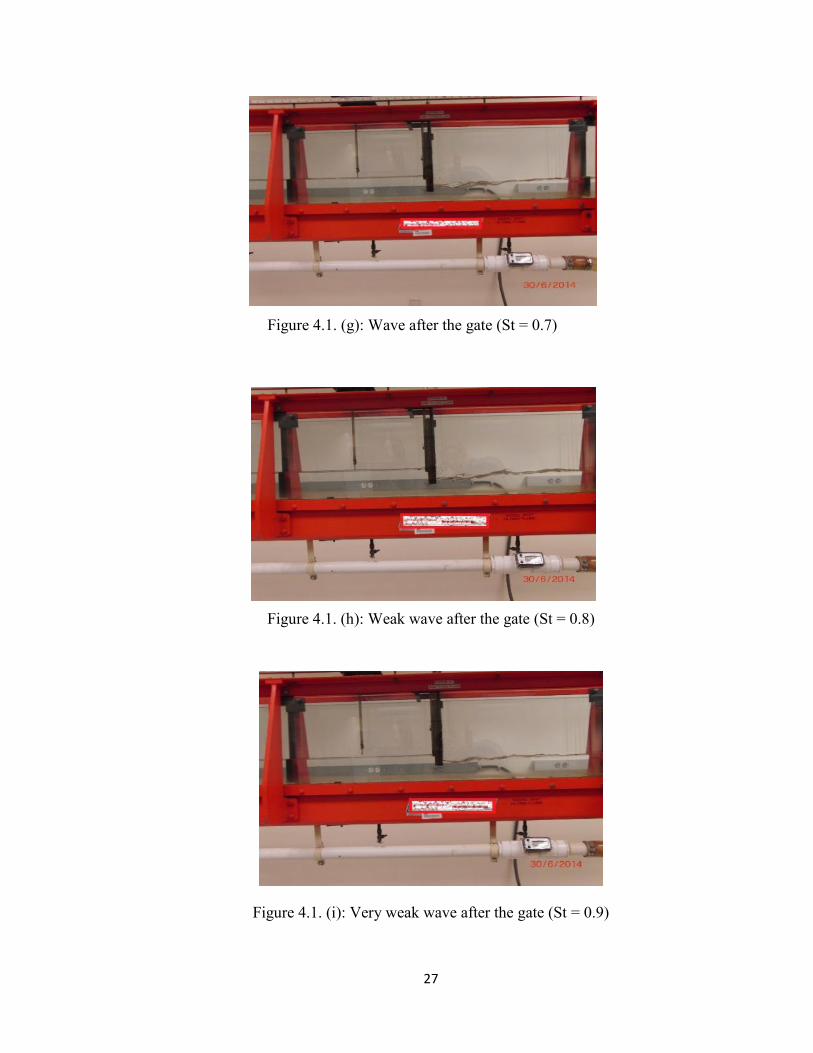
4.1. (g) Wave after the gate (St = 0.7) ............................................................................ 27
4.1. (h) Weak wave after the gate (St = 0.8) ................................................................... 27
4.1. (i) Very weak wave after the gate (St = 0.9) ............................................................ 27
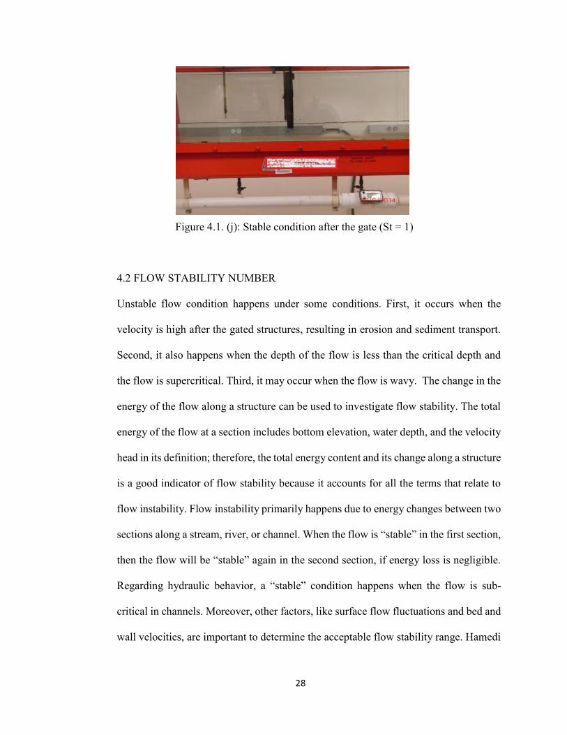
4.1. (j) Stable condition after the gate (St = 1) ............................................................... 28
4.2. (a) Sections in hydraulic jump ................................................................................. 30
4.2. (b) Sections in subcritical flow ................................................................................ 30
4.3 A method to calculate the Flow Stability Number.................................................... 31
4.4. (a) Vertical gate........................................................................................................ 34
4.4. (b) Gate with Expansion .......................................................................................... 34
4.4. (c) Gate with Contraction......................................................................................... 34
4.5 Flume and gate .......................................................................................................... 35
4.6. (a) Gate with Expansion, section view .................................................................... 36
4.6. (b) Gate with Expansion, plan view ......................................................................... 37
4.7. (a) Gate with Contraction, section view .................................................................. 37
4.7. (b) Gate with Contraction, plan view ....................................................................... 38
4.8 The flume and lagoon, satellite view ........................................................................ 39
4.9. (a) The first valve ..................................................................................................... 39
4.9. (b) The second valve ................................................................................................ 40
4.10 The flume ................................................................................................................ 40
4.11 The mixture which covers the flume bed ................................................................ 41
4.12. (a) An overview of the gate ................................................................................... 42
4.12. (b) Details of the gate ............................................................................................. 43
4.13. (a) Gate with Expansion, section view .................................................................. 44
4.13. (b) Gate with Expansion, plan view ....................................................................... 44
4.14. (a) Gate with Contraction, section view ................................................................ 45
4.14. (b) Gate with Contraction, plan view ..................................................................... 45
4.15 Digital flow meter ................................................................................................... 46
4.16 Digital velocity meter ............................................................................................. 50
4.17 Digital thermometer ................................................................................................ 51
4.18. (a) A high-speed camera and tripod ....................................................................... 52
4.18. (b) 1000 lumen LED portable work light .............................................................. 53
5.1.1 Free flow under the vertical sluice gate ................................................................. 58
5.1.2 Submerged flow under the vertical sluice gate ...................................................... 59
xiv
5.1.3 Neural Network, MLP ........................................................................................... 61
5.1.4. (a) Hydraulic jump after the gate (St = 0) ............................................................. 66
5.1.4. (b) Submerged hydraulic jump after the gate (St = 0.2) ....................................... 67
5.1.4. (c) Strong wave after the gate (St = 0.6) ............................................................... 67
5.1.4. (d) Stable condition after the gate (St = 1) ............................................................ 67
5.1.5 h0/a - dc/h0 graph .................................................................................................... 69
5.1.6 Post-processing - regression – ANN ...................................................................... 71
5.1.7 RMSE – Post-processing ....................................................................................... 74
5.2.1. (a) Supercritical flow after the gate ...................................................................... 77
5.2.1. (b) Subcritical flow after the gate ......................................................................... 78
5.2.2 Boxplots – sections 2 and 3 ................................................................................... 81
5.2.3 Normal Q-Q plot – section 2 .................................................................................. 81
5.2.4 Normal Q-Q plot – section 3 .................................................................................. 82
5.2.5 Q-Q plot – section 2 versus section 3 .................................................................... 82
5.2.6. (a) Sediment transport after the gate ..................................................................... 86
5.2.6. (b) Surface flow fluctuations after the gate ........................................................... 86
5.2.7 Boxplots – sections 2 and 3 ................................................................................... 90
5.2.8 Normal Q-Q plot – section 2 .................................................................................. 90
5.2.9 Normal Q-Q plot – section 3 .................................................................................. 91
5.2.10 Q-Q plot – section 2 versus section 3 .................................................................. 91
5.3.1 Sections in a gate with expansion .......................................................................... 96
5.3.2. (a) Flow fluctuations after a gate with expansion ................................................. 97
5.3.2. (b) Stable flow after a gate with expansion .......................................................... 97
5.3.3 Boxplots – sections 2 and 3 ................................................................................. 101
5.3.4 Normal Q-Q plot – section 2 ................................................................................ 101
5.3.5 Normal Q-Q plot – section 3 ................................................................................ 102
5.3.6 Q-Q plot – section 2 versus section 3 .................................................................. 102
5.3.7 h0/a vs. dc/h0......................................................................................................... 105
5.3.8. (a) Sediment transport in the presence of a gate with expansion ........................ 107
5.3.8. (b) Flow pattern in the presence of a gate with expansion .................................. 107
5.3.9 Boxplots – sections 2 and 3 ................................................................................. 111
5.3.10 Normal Q-Q plot – section 2 .............................................................................. 111
5.3.11 Normal Q-Q plot – section 3 .............................................................................. 112
5.3.12 Q-Q plot – section 2 versus section 3 ................................................................ 112
5.4.1 Sections in a gate with contraction ...................................................................... 117
5.4.2. (a) Flow fluctuations in the presence of a gate with contractions....................... 118
5.4.2. (b) Stable flow in the presence of a gate with contractions ................................ 118
5.4.3 Boxplots – sections 2 and 3 ................................................................................. 122
5.4.4 Normal Q-Q plot – section 2 ................................................................................ 122
5.4.5 Normal Q-Q plot – section 3 ................................................................................ 123
5.4.6 Q-Q plot – section 2 versus section 3 .................................................................. 123
5.4.7 h0/a vs. dc/h0......................................................................................................... 126
xv
5.4.8. (a) Sediment transport in the presence of a gate with contractions .................... 128
5.4.8. (b) Flow pattern in the presence of a gate with contractions .............................. 128
5.4.9 Boxplots – sections 2 and 3 ................................................................................. 132
5.4.10 Normal Q-Q plot – section 2 .............................................................................. 132
5.4.11 Normal Q-Q plot – section 3 .............................................................................. 133
5.4.12 Q-Q plot – section 2 versus section 3 ................................................................ 133
5.5.1 Stability versus discharge in a gate ...................................................................... 138
5.5.2 Stability versus discharge in a gate with expansion ............................................. 139
5.5.3 Stability versus discharge in a gate with contraction ........................................... 140
5.5.4 h0/a versus dc/h0 in all three hydraulic structures ................................................ 143
5.5.5 Schematic of the river .......................................................................................... 151
5.5.6 Benefits to each agency in different situations .................................................... 152
5.5.7 Scale effect in gates ............................................................................................. 154
5.5.8 Scale effect in a gate with expansion ................................................................... 155
5.5.9 Scale effect in a gate with contraction ................................................................. 155
5.6.1 Image histogram on a 0-1 scale ........................................................................... 159
5.6.2. (a) Stepped spillway physical model, the Water Research Institute ................... 161
5.6.2. (b) Top view, stepped spillway, the Water Research Institute .......................... 161
5.6.3. (a) Top view, Spillway Park – Lake Worth, FL, [Google Earth] ....................... 163
5.6.3. (b) Image histogram – section one ...................................................................... 164
5.6.3. (c) Image histogram – section two ...................................................................... 164
5.6.3. (d) Image histogram – section three.................................................................... 165
5.6.3. (e) Downstream flow condition .......................................................................... 165
5.6.4. (a) Top view, Oroville Dam – CA, [Google Earth] ............................................ 167
5.6.4. (b) Section one .................................................................................................... 168
5.6.4. (c) Sections two and three ................................................................................... 168
5.6.4. (d) Image histogram – section one ...................................................................... 169
5.6.4. (e) Image histogram – section two ...................................................................... 169
5.6.4. (f) Image histogram – section three .................................................................... 170
B.1 Grain Size Distribution Curve ................................................................................ 197
G.1 Gate hydraulic structure (S334) ............................................................................. 220
G.2 Downstream of the hydraulic structure (S334) ...................................................... 220
G.3 Upstream of the hydraulic structure (S334) ........................................................... 221
G.4 Flow condition immediately after a gate (S334) .................................................... 221
G.5 Depth measurement................................................................................................ 222
G.6 Upstream of the hydraulic structure (S333) ........................................................... 222
G.7 Flow in the canal .................................................................................................... 223
G.8 The gate hydraulic structure (S355B) .................................................................... 223
G.9 Details of the gate hydraulic structure (S355B) ..................................................... 224
G.10 Upstream of the gate hydraulic structure (S355B)............................................... 224
xvi
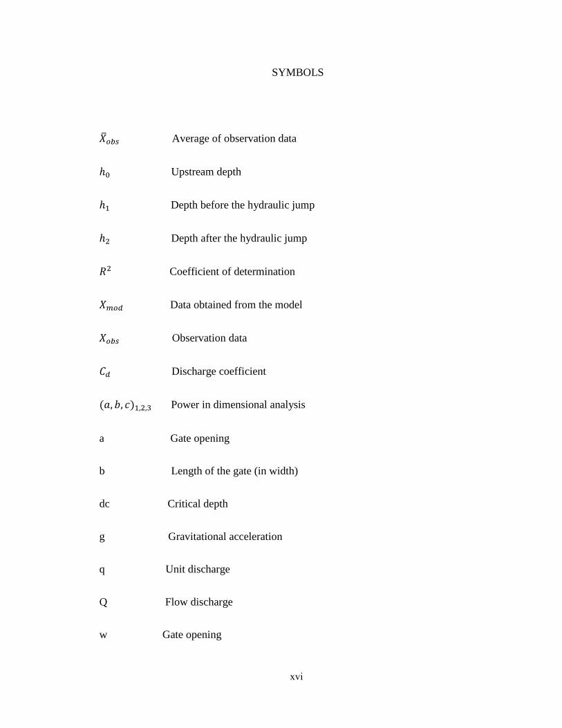
SYMBOLS
�̅�𝑜𝑏𝑠 Average of observation data
ℎ0 Upstream depth
ℎ1 Depth before the hydraulic jump
ℎ2 Depth after the hydraulic jump
𝑅2 Coefficient of determination
𝑋𝑚𝑜𝑑 Data obtained from the model
𝑋𝑜𝑏𝑠 Observation data
𝐶𝑑 Discharge coefficient
(𝑎, 𝑏, 𝑐)1,2,3 Power in dimensional analysis
a Gate opening
b Length of the gate (in width)
dc Critical depth
g Gravitational acceleration
q Unit discharge
Q Flow discharge
w Gate opening
xvii
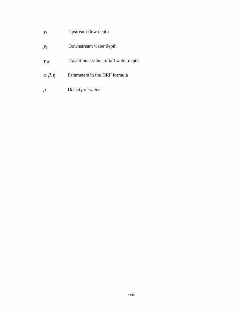
𝑦1 Upstream flow depth
𝑦3 Downstream water depth
𝑦3𝑡 Transitional value of tail water depth
𝛼, 𝛽, 𝜂 Parameters in the DRF formula
𝜌 Density of water
xviii
ABBREVIATIONS AND ACRONYMS
ANN Artificial Neural Network
DRF Discharge Reduction Factor
E Nash-Sutcliffe Coefficient
GPM Gallons per minute
L Length in dimension analysis
M Mass in dimension analysis
MLP Multi-Layer Perceptron
n Number of observed data points used to calculate RMSE
NLPCA Nonlinear principal component analysis
PCA Principal component analysis
r Basic (main) parameters in the dimension analysis
RMSE Root mean square error
St Flow Stability Factor
T Time in dimension analysis
𝑘 All parameters in dimension analysis
𝜋 Buckingham Method

1
DISCLAIMER
The author, Professor Hector R. Fuentes, Florida International University, the Civil and
Environmental Engineering Graduate Program, and all other technical sources referred to
in this report:
1. Do not make any warranty or representation, expressed or implied, with respect to the
accuracy and completeness of the information contained in this report.
2. Do not warrant that the use of any information, method, or process described in this
report may not infringe on privately owned rights; and
3. Do not assume any liability with respect to the use of or for damages resulting from the
use of any information, method, or process described in this report.
This dissertation does not reflect the official views or policies of any sponsoring or
participating organizations and individuals.
2
CHAPTER 1
INTRODUCTION
Streams, rivers, and canals are able to transfer flow from one point to another. Along
their pathways, they can be used for different purposes, such as water supply,
recreation, fisheries, and agricultural irrigation, etc. Hydraulic structures are usually
built along streams, rivers, and canals to manage and control the flow, including, for
instance, maintaining the upstream level to ensure that irrigation needs are met.
Despite the advantages of hydraulic structures, they also have disadvantages that may
be reduced by a better understanding of flow conditions and their control. A vertical
gate is one type of hydraulic structure. When the gate opening is small, downstream
the flow has a high velocity and flow fluctuation, which causes erosion downstream of
the gate.
If the main causes of erosion (and the resulting sediment transport) downstream of gates
need to be controlled, a flow classification method is helpful in minimizing erosion.
Although a few flow classification methods have been developed via past research,
none has fully aided in minimizing erosion after gates. Consequently, there is a need to
develop a new flow classification method that can aid in identifying desired flow
conditions. This is stable flow.
Two flow classification methods have been introduced in this research. The first one
classifies flow based on the Flow Stability Factor and the second one classifies flow
based on the Flow Stability Number (which is dimensionless). The gated structures
3
should be managed in a way that the downstream condition is very close to the stable
condition, thus minimizing undesirable flow conditions.
This research focuses on three gated structures including a gate, a gate with expansion,
and a gate with contraction. These structures were investigated in two laboratories, and
at different scales, to address a possible scale effect on the methodologies herein
developed. These structures were investigated over a range of discharges and
thicknesses (for both gates with expansion and contraction). Consequently, they can be
compared under flow to select the best structure type to ensure a stable flow.
Six chapters of this dissertation present and analyze numerous research questions. The
first chapter is an introduction and describes the needs, problems, and probable
solutions; it also outlines the overall structure of the dissertation. The second chapter
documents the literature review and defines gaps in the existing knowledge. Objectives
are defined in the third chapter. The methods that are used in the research, laboratories,
variables, instruments, and the accuracy of results are detailed in chapter four.
The fifth chapter includes results and a discussion, covering seven sections. The Flow
Stability Factor is defined in the first section and its application in vertical gates is also
demonstrated in that section. The second, third, and fourth sections show the
applications of the Flow Stability Number in a gate, a gate with expansion, and a gate
with contraction, respectively. The accuracy of the Flow Stability Factor was compared
with the Flow Stability Number in section five; the three studied structures were also
compared in this section. A method that uses Game Theory and the Nash Equilibrium
was implemented to select the best structure for specific flow conditions. A scale effect
and the probable causes of a scale effect in this research were also discussed in the last
4
part of section five. Section six introduces the Efficiency Index as an innovative index
which is practical, low-cost, and quick to apply. This index can be determined using an
image processing technique and is able to estimate the overall efficiency of hydraulic
structures. Two case studies were presented in this section to show the application of
this method. Section seven, which is the last section of chapter five, documented the
limitations of the methods used in these investigations.
Chapter six, the last chapter, includes both conclusions and recommendations for future
research. In addition, supporting data and information regarding permissible velocity,
bed materials, and flow stability, as well as pictures of real scale structures, are
provided in the Appendices.
5
CHAPTER 2
BACKGROUND
2.1 LITERATURE REVIEW
Sluice gates are primarily used to control the upstream depth to provide required water
for irrigation and to manage passing discharge below gates in channels [1 - 14]. A wide
range of sluice gate characteristics has been considered by researchers in different parts
of the world during past decades. The geographic distribution, as well as the timeline
of these studies, are reported in the first and second parts of the literature review in this
chapter (2.1.1 and 2.1.2). The geographical distribution includes a statistical analysis
to show the contributing percentage of sluice gates studies from each country. The
timeline distribution reports relevant research work on the sluice gate from the 19th
century to the present day differentiated by continent and country. Gate studies can be
categorized as either old or new studies. Old studies are those published before 1900
and from 1900 to 1949. New studies are divided into three time periods: 1950 to 1979,
1980 to 1999, and finally 2000 to 2017. The results indicate that most studies belong
to the two most recent time periods (new studies). There are some old studies which
were published prior to 1900 [15 - 18]. The oldest study was published in 1848 by
Boileau [15]. Also, some other studies were published in the first half of the 20th century
[19 - 29]. New studies started with Henry [30] in 1950 and were followed by other
research from 1959 [31 - 36] and 1960 to 1969 [37 - 44]. The final part of this chapter
illustrates the most popular subjects in sluice gate studies and briefly explains other
researchers’ work. It should be noted that all data has been collected from research
6
scholars, including conference and journal papers, books, journal discussions, and
closures to journal discussions and handbooks.
In the initial stage, more than 150 pieces of research were collected and briefly
considered to prepare the sluice gate research database; this was then narrowed down
to 71 works for further consideration based on their relevance to this topic of study.
2.1.1 Geographic Distribution
Research has been conducted to show the geographical distribution of studies related
to sluice gates. Each continent was considered separately and then a statistical analysis
was conducted for each country based on the number of publications and the number
of researchers.
Based on the database which has been used in this research, in total 21 countries (the
UK is counted as a single country) have contributed to sluice gate research studies.
These countries are from all the continents. This means that the topic is important
globally and that researchers are paying attention to gate issues. It should be noted that
some gate research may have been conducted in other countries. However, these works
are not found in research journals. The author did try to include all important and
relevant work in the database. The criteria for considering the research in the statistical
results are the first author and the institute/school of the first author when he/she
published the work. Therefore, the nationality of the first author was not considered in
the statistical analysis.
7
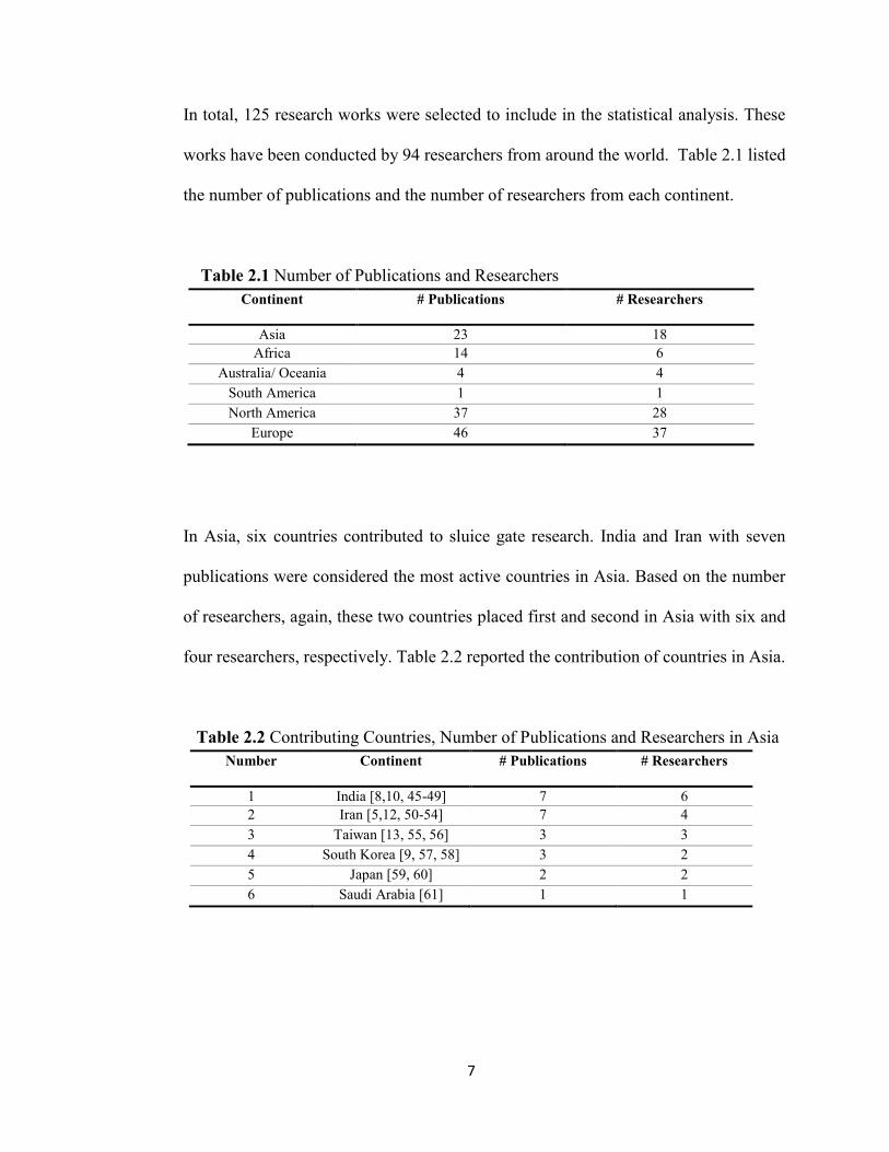
In total, 125 research works were selected to include in the statistical analysis. These
works have been conducted by 94 researchers from around the world. Table 2.1 listed
the number of publications and the number of researchers from each continent.
Table 2.1 Number of Publications and Researchers Continent # Publications # Researchers
Asia 23 18 Africa 14 6
Australia/ Oceania 4 4 South America 1 1 North America 37 28
Europe 46 37
In Asia, six countries contributed to sluice gate research. India and Iran with seven
publications were considered the most active countries in Asia. Based on the number
of researchers, again, these two countries placed first and second in Asia with six and
four researchers, respectively. Table 2.2 reported the contribution of countries in Asia.
Table 2.2 Contributing Countries, Number of Publications and Researchers in Asia Number Continent # Publications # Researchers
1 India [8,10, 45-49] 7 6 2 Iran [5,12, 50-54] 7 4 3 Taiwan [13, 55, 56] 3 3 4 South Korea [9, 57, 58] 3 2 5 Japan [59, 60] 2 2 6 Saudi Arabia [61] 1 1
8
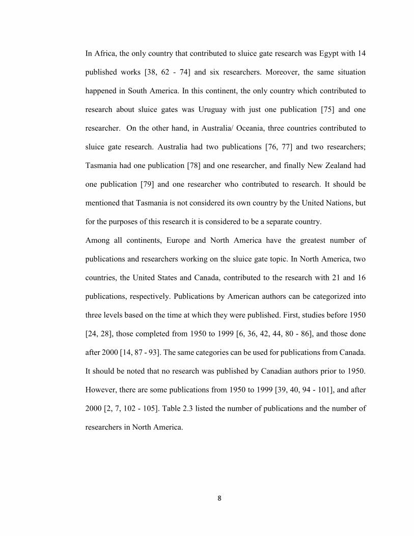
In Africa, the only country that contributed to sluice gate research was Egypt with 14
published works [38, 62 - 74] and six researchers. Moreover, the same situation
happened in South America. In this continent, the only country which contributed to
research about sluice gates was Uruguay with just one publication [75] and one
researcher. On the other hand, in Australia/ Oceania, three countries contributed to
sluice gate research. Australia had two publications [76, 77] and two researchers;
Tasmania had one publication [78] and one researcher, and finally New Zealand had
one publication [79] and one researcher who contributed to research. It should be
mentioned that Tasmania is not considered its own country by the United Nations, but
for the purposes of this research it is considered to be a separate country.
Among all continents, Europe and North America have the greatest number of
publications and researchers working on the sluice gate topic. In North America, two
countries, the United States and Canada, contributed to the research with 21 and 16
publications, respectively. Publications by American authors can be categorized into
three levels based on the time at which they were published. First, studies before 1950
[24, 28], those completed from 1950 to 1999 [6, 36, 42, 44, 80 - 86], and those done
after 2000 [14, 87 - 93]. The same categories can be used for publications from Canada.
It should be noted that no research was published by Canadian authors prior to 1950.
However, there are some publications from 1950 to 1999 [39, 40, 94 - 101], and after
2000 [2, 7, 102 - 105]. Table 2.3 listed the number of publications and the number of
researchers in North America.
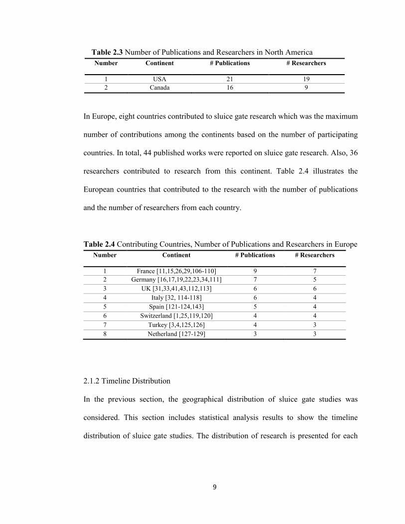
9
Table 2.3 Number of Publications and Researchers in North America Number Continent # Publications # Researchers
1 USA 21 19 2 Canada 16 9
In Europe, eight countries contributed to sluice gate research which was the maximum
number of contributions among the continents based on the number of participating
countries. In total, 44 published works were reported on sluice gate research. Also, 36
researchers contributed to research from this continent. Table 2.4 illustrates the
European countries that contributed to the research with the number of publications
and the number of researchers from each country.
Table 2.4 Contributing Countries, Number of Publications and Researchers in Europe Number Continent # Publications # Researchers
1 France [11,15,26,29,106-110] 9 7 2 Germany [16,17,19,22,23,34,111] 7 5 3 UK [31,33,41,43,112,113] 6 6 4 Italy [32, 114-118] 6 4 5 Spain [121-124,143] 5 4 6 Switzerland [1,25,119,120] 4 4 7 Turkey [3,4,125,126] 4 3 8 Netherland [127-129] 3 3
2.1.2 Timeline Distribution
In the previous section, the geographical distribution of sluice gate studies was
considered. This section includes statistical analysis results to show the timeline
distribution of sluice gate studies. The distribution of research is presented for each

10
country by decade. In total, 144 research works have been included in this statistical
analysis. Table 2.5 shows the contribution of each country in different decades.
Table 2.5 Countries’ Contribution from Each Decade Country 2010-
2017
2000-
2009
1990-
1999
1980-
1989
1970-
1979
1960-
1969
1950-
1959
1940-
1949
1930-
1939
Before
1930
USA 1 7 2 3 2 3 1 1 1 - Canada 2 4 2 4 2 2 - - - - Uruguay 1 - - - - - - - - - Egypt - 1 11 1 - 1 - - - - Australia - - 1 - 1 - - - - - Tasmania - - - - 1 - - - - - New Zealand
- - 1 - - - - - - - India - 1 4 2 - - - - - - Taiwan - 2 - - 1 - - - - - South Korea
2 1 - - - - - - - - Japan - - 1 - 1 - - - - - Iran 4 2 1 - - - - - - - Saudi Arabia
- - 1 - - - - - - - France 2 4 - - - - - 1 1 1 Germany - - - - 1 - 1 - 2 3 UK - - 1 - 1 2 2 - - - Italy - 3 1 - 1 - 1 - - - Switzerland 1 - 2 - - - - - 1 - Spain 4 1 - - - - - - - - Netherland - 1 2 - - - - - - - Turkey 1 2 - 1 - - - - - -
From Table 2.5, it can be inferred that Iran and Spain have the most contributions in
the 2010-2017 period with four publications. The United States had the maximum
number of contributions in the 2000-2009 period with seven publications, and Egypt
had the greatest number of publications (11) during the 1990-1999 period. France and
Germany had the most contributions in the initial stage of the studies (1930-1939 and
11
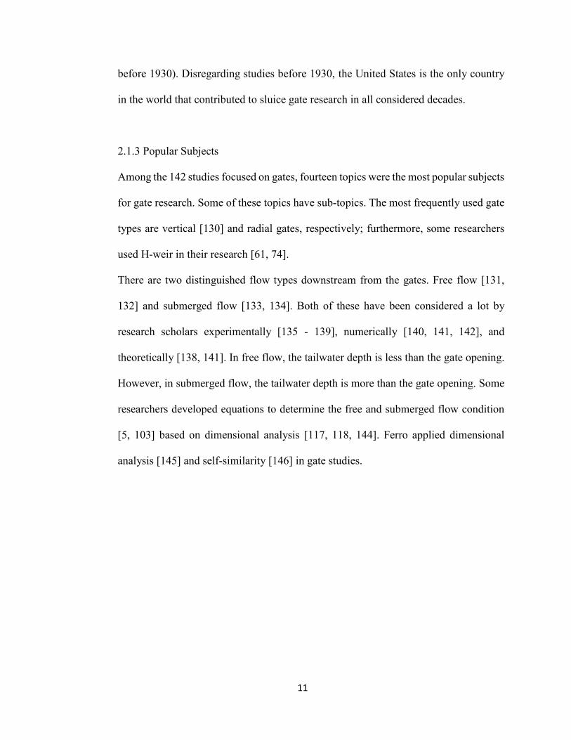
before 1930). Disregarding studies before 1930, the United States is the only country
in the world that contributed to sluice gate research in all considered decades.
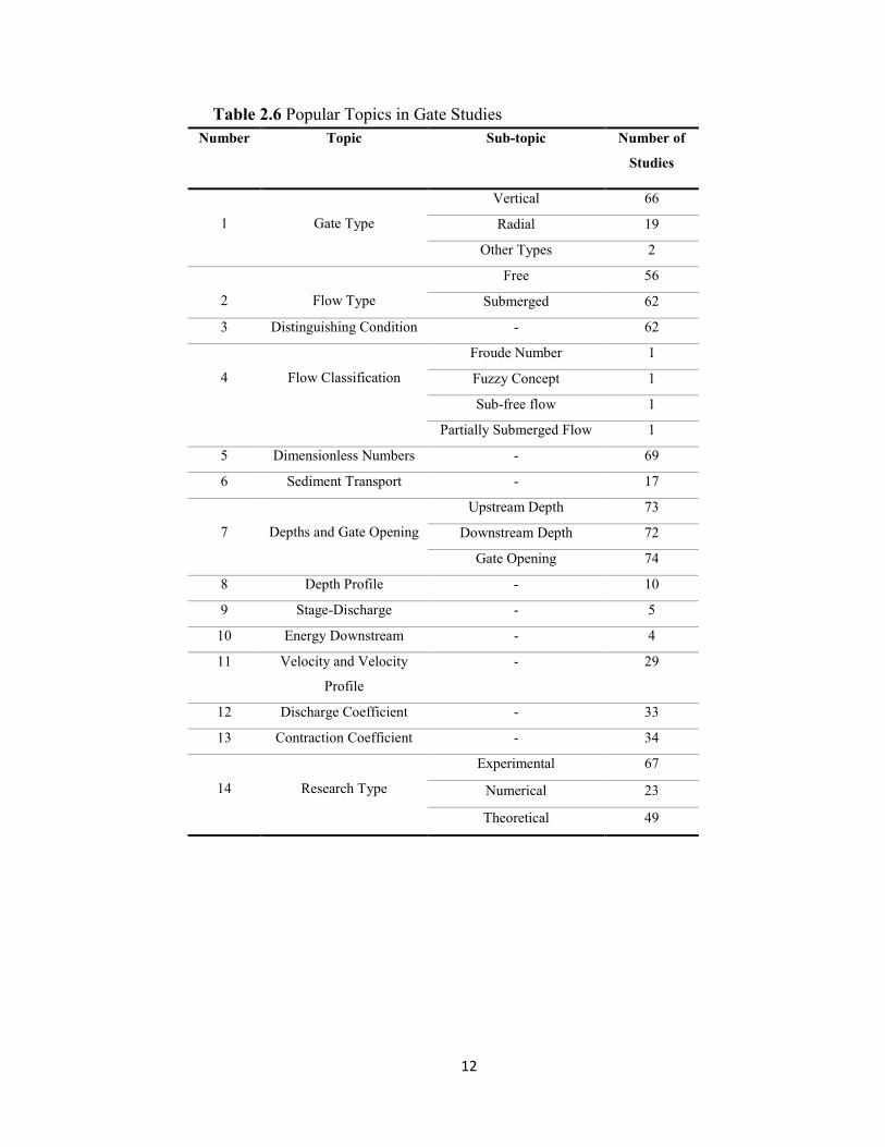
2.1.3 Popular Subjects
Among the 142 studies focused on gates, fourteen topics were the most popular subjects
for gate research. Some of these topics have sub-topics. The most frequently used gate
types are vertical [130] and radial gates, respectively; furthermore, some researchers
used H-weir in their research [61, 74].
There are two distinguished flow types downstream from the gates. Free flow [131,
132] and submerged flow [133, 134]. Both of these have been considered a lot by
research scholars experimentally [135 - 139], numerically [140, 141, 142], and
theoretically [138, 141]. In free flow, the tailwater depth is less than the gate opening.
However, in submerged flow, the tailwater depth is more than the gate opening. Some
researchers developed equations to determine the free and submerged flow condition
[5, 103] based on dimensional analysis [117, 118, 144]. Ferro applied dimensional
analysis [145] and self-similarity [146] in gate studies.
12
Table 2.6 Popular Topics in Gate Studies Number Topic Sub-topic Number of
Studies
1
Gate Type
Vertical 66
Radial 19
Other Types 2
2
Flow Type
Free 56
Submerged 62
3 Distinguishing Condition - 62
4
Flow Classification
Froude Number 1
Fuzzy Concept 1
Sub-free flow 1
Partially Submerged Flow 1
5 Dimensionless Numbers - 69
6 Sediment Transport - 17
7
Depths and Gate Opening
Upstream Depth 73
Downstream Depth 72
Gate Opening 74
8 Depth Profile - 10
9 Stage-Discharge - 5
10 Energy Downstream - 4
11 Velocity and Velocity
Profile
- 29
12 Discharge Coefficient - 33
13 Contraction Coefficient - 34
14
Research Type
Experimental 67
Numerical 23
Theoretical 49
13
Upstream depth, tailwater, and gate opening are the most common variables which
have been used in the dimensional analysis of gate studies [2, 5, 10, 14, 55]. Yen et al.
[13] studied maximum gate openings in vertical gates in rectangular canals. They noted
that supercritical flow occurs exactly after the gate in the downstream section when the
gate opening is smaller than the critical depth. Furthermore, the Froude number has
been considered by some researchers in dimensional analysis [9, 59, 62, 115].
Some researchers have tried to classify the flow regime downstream of the gate.
Hamedi and Fuentes used the Fuzzy Concept to classify the flow [14]. In their research,
the number zero was assigned to a hydraulic jump. It means that the flow was
completely unstable, and the number one was assigned to a stable condition. Belaud et
al. [106] plotted the submergence ratio versus the relative gate opening and defined
three flow types downstream of the gate. These three flow types are free flow, partially
submerged flow, and submerged flow. The partially submerged flow can be seen
between the other two flow types. Defina and Susin [115] related flow and gate opening
under the vertical gates to the Froude number. With a Froude number greater than 0.8,
the flow behavior is like a hysteresis, due to the contraction effect under the gate.
Bhowmik [81], also, classified different types of a hydraulic jump based on the Froude
number. Moreover, Vanden-Broeck [80] assumed an incompressible fluid. He
mentioned that when the Froude number is large downstream, negligible waves occur,
and the flow is mostly smooth upstream. However, when the Froude number is small
downstream, large waves occur.
14
Sediment transport downstream of the gate is another topic which has been considered
by some researchers. A moderate number of publications have paid attention to this
topic. Bove et al. [75] used PIV (Particle Image Velocimetry) to consider sediment
transport in non-cohesive particle sediment beds after the gate. They observed two
holes downstream of the gate and reported that the first hole is made because of the
shear stress of the jet flow, whereas the second hole is made because of turbulent
fluctuations which happened due to jet flow destabilization. Therefore, the production
mechanism of these holes is completely different. Furthermore, Kells et al. [102]
considered the effect of grain size downstream of the gate on the dynamics of the local
scour process in the submerged flow. They noted that the area and depth of the scours
are dependent on grain size. Smaller grain size produces larger scours. They, also,
reported that the smaller scour had been seen when a mixed bed was used (compared
with a uniform grain). Moreover, in the presence of higher discharges and tailwater,
the maximum scour depth is increasing.
Another popular topic among researchers is determining stage-discharge relationships
in gates. Shahrokhnia and Javan used dimensional analysis and presented some
relationships for determining the stage-discharge relationship in radial gates for both
free and submerged flow conditions. They pointed out that the Reynolds number has a
negligible effect on average discharge. Therefore, it can be disregarded. They also
claimed that their method was better than conventional ones for determining the stage-
discharge relationship in radial gates [12]. Bijankhan et al. determined that the methods
to obtain the stage-discharge relationships under gates are suitable for free flow, but
need to be reconsidered for a low submerged condition [5]. They presented a method
15
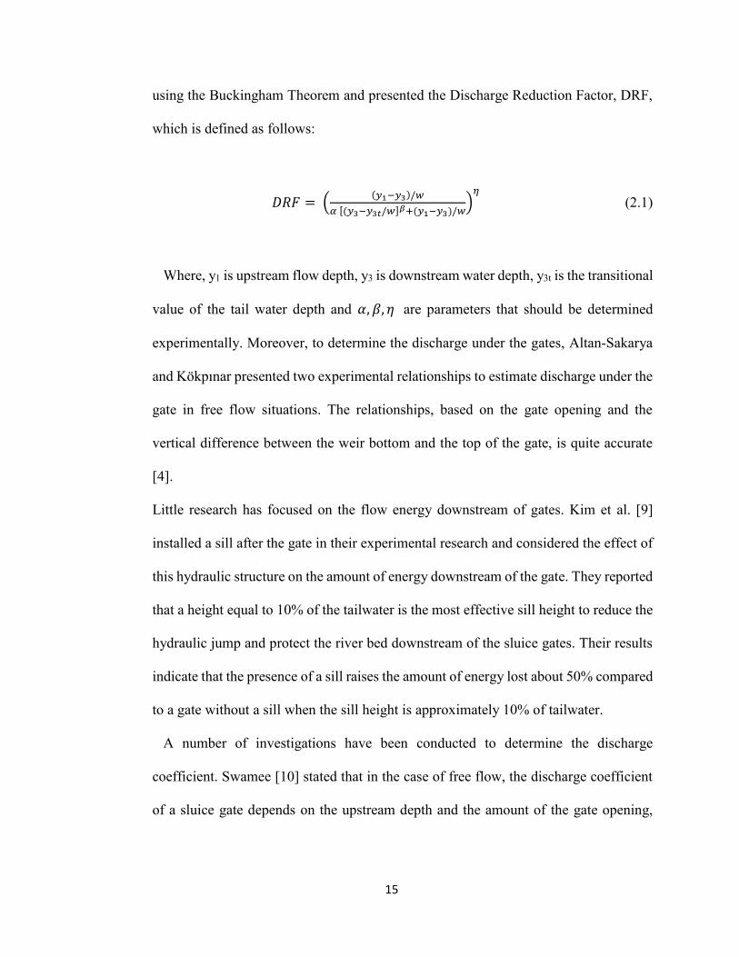
using the Buckingham Theorem and presented the Discharge Reduction Factor, DRF,
which is defined as follows:
𝐷𝑅𝐹 = ((𝑦1−𝑦3)/𝑤
𝛼 [(𝑦3−𝑦3𝑡/𝑤]𝛽+(𝑦1−𝑦3)/𝑤)
𝜂
(2.1)
Where, y1 is upstream flow depth, y3 is downstream water depth, y3t is the transitional
value of the tail water depth and 𝛼, 𝛽, 𝜂 are parameters that should be determined
experimentally. Moreover, to determine the discharge under the gates, Altan-Sakarya
and Kökpınar presented two experimental relationships to estimate discharge under the
gate in free flow situations. The relationships, based on the gate opening and the
vertical difference between the weir bottom and the top of the gate, is quite accurate
[4].
Little research has focused on the flow energy downstream of gates. Kim et al. [9]
installed a sill after the gate in their experimental research and considered the effect of
this hydraulic structure on the amount of energy downstream of the gate. They reported
that a height equal to 10% of the tailwater is the most effective sill height to reduce the
hydraulic jump and protect the river bed downstream of the sluice gates. Their results
indicate that the presence of a sill raises the amount of energy lost about 50% compared
to a gate without a sill when the sill height is approximately 10% of tailwater.
A number of investigations have been conducted to determine the discharge
coefficient. Swamee [10] stated that in the case of free flow, the discharge coefficient
of a sluice gate depends on the upstream depth and the amount of the gate opening,
16
whereas in a submerged flow, the discharge coefficient depends on the tailwater depth,
as well as the factors mentioned for free flow. This researcher proposed a new method
to attain the discharge coefficient as a function of the gate opening. He also believed
that previous graphical methods that determined the discharge coefficient using the
upstream depth to gate opening ratio graphs under free flow conditions were not strong
enough to use in numerical and analytical methods. Habibzadeh et al. utilized formulas
to determine the discharge coefficient under gates under both free and submerged flow
conditions. They accounted for the energy lost between the upstream section and the
venna section (immediately after the gate) in the discharge coefficient. They also
acknowledged that energy loss is a function of gate geometry, and can thus change the
discharge coefficient. Their formula can be used to determine the discharge coefficient
in gates with different shapes [103].
The contraction coefficient is one of the important parameters in sluice gate studies.
Belaud et al. considered the contraction coefficient under gates in both free and
submerged flow conditions. They determined that when the gate opening is small the
contraction coefficient is approximately the same for free and submerged flow
conditions. However, the gate opening is larger [106].
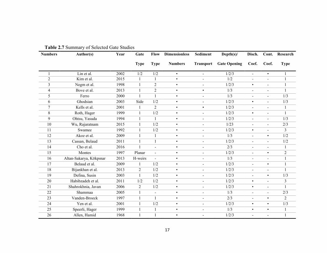
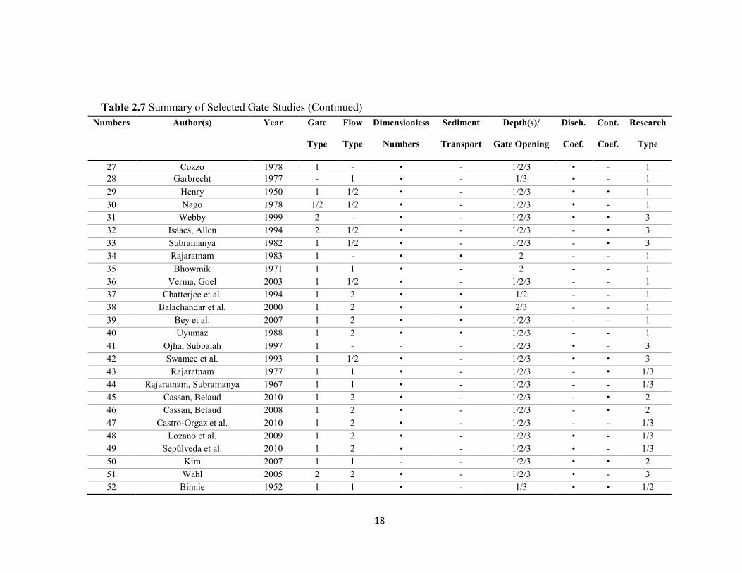
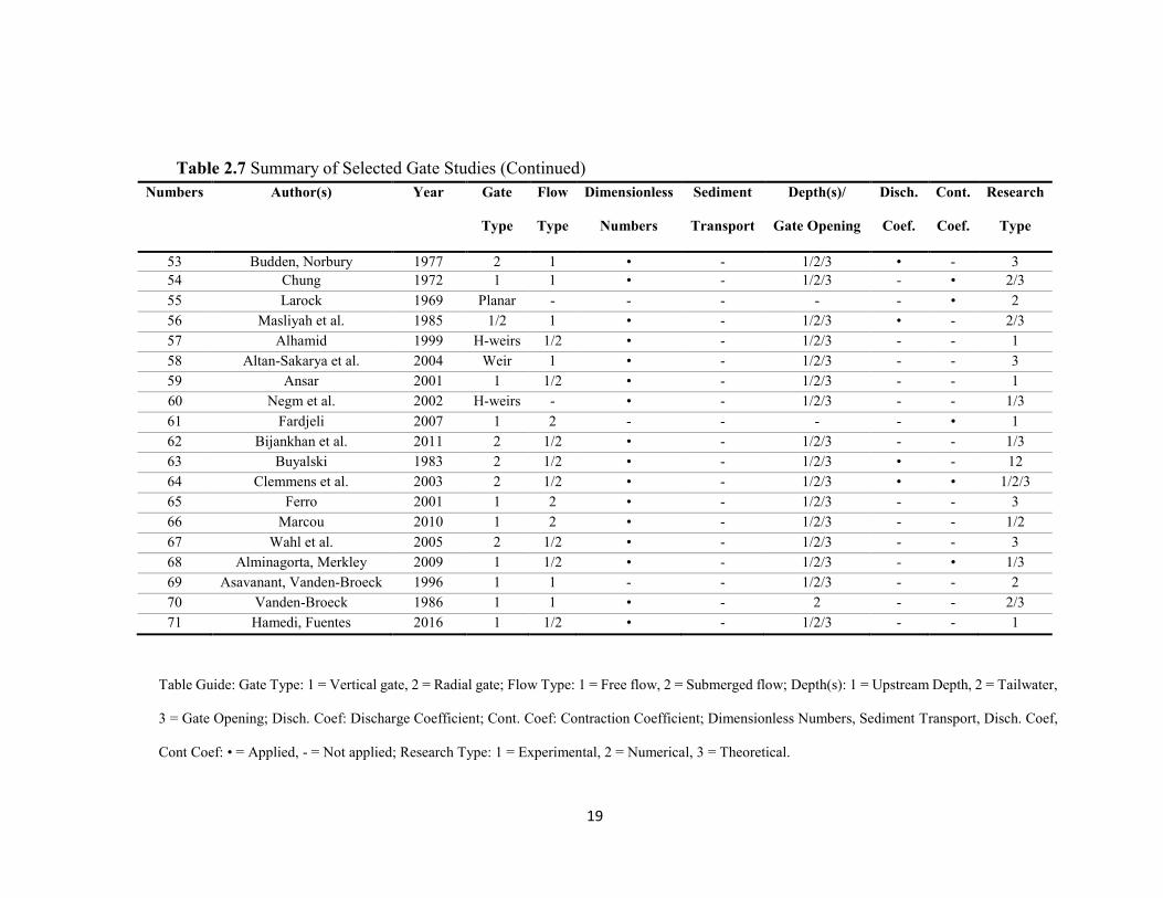
There are lots of studies on each topic. Therefore, a summary of important studies is
listed in Table 2.7. This table illustrates the authors, the year, and the contribution of
each selected publication to different popular topics of sluice gate studies.
17
Table 2.7 Summary of Selected Gate Studies Numbers Author(s) Year Gate
Type
Flow
Type
Dimensionless
Numbers
Sediment
Transport
Depth(s)/
Gate Opening
Disch.
Coef.
Cont.
Coef.
Research
Type
1 Lin et al. 2002 1/2 1/2 • - 1/2/3 - • 1 2 Kim et al. 2015 1 1 • - 1/2 - - 1 3 Negm et al. 1998 1 2 • - 1/2/3 • - 1 4 Bove et al. 2013 1 2 • • 1/3 - - 1 5 Ferro 2000 1 1 • - 1/3 - - 1/3 6 Ghodsian 2003 Side 1/2 • - 1/2/3 • - 1/3 7 Kells et al. 2001 1 2 • • 1/2/3 - - 1 8 Roth, Hager 1999 1 1/2 • - 1/2/3 • - 1 9 Ohtsu, Yasuda 1994 1 1 • - 1/2/3 - - 1/3 10 Wu, Rajaratnam 2015 1 1/2 • - 1/23 - - 2/3 11 Swamee 1992 1 1/2 • - 1/2/3 • - 3 12 Akoz et al. 2009 1 1 • - 1/3 - • 1/2 13 Cassan, Belaud 2011 1 1 • - 1/2/3 - - 1/2 14 Cho et al. 2016 1 - • - 2/3 - - 1 15 Montes 1997 Planar - • - 1/2/3 - • 2 16 Altan-Sakarya, Kökpınar 2013 H-weirs - • - 1/3 - - 1 17 Belaud et al. 2009 1 1/2 • - 1/2/3 - • 1 18 Bijankhan et al. 2013 2 1/2 • - 1/2/3 - - 1 19 Defina, Susin 2003 1 1/2 • - 1/2/3 - • 1/3 20 Habibzadeh et al. 2011 1/2 1/2 • - 1/2/3 • - 3 21 Shahrokhnia, Javan 2006 2 1/2 • - 1/2/3 • - 1 22 Shammaa 2005 1 - • - 1/3 - - 2/3 23 Vanden-Broeck
1997 1 1 • - 2/3 - • 2 24 Yen et al. 2001 1 1/2 • - 1/2/3 • • 1/3 25 Speerli, Hager 1999 1 1 • - 1/3 • • 1 26 Allen, Hamid 1968 1 1 • - 1/2/3 - - 1
18
Table 2.7 Summary of Selected Gate Studies (Continued) Numbers Author(s) Year Gate
Type
Flow
Type
Dimensionless
Numbers
Sediment
Transport
Depth(s)/
Gate Opening
Disch.
Coef.
Cont.
Coef.
Research
Type
27 Cozzo 1978 1 - • - 1/2/3 • - 1 28 Garbrecht 1977 - 1 • - 1/3 • - 1 29 Henry 1950 1 1/2 • - 1/2/3 • • 1 30 Nago 1978 1/2 1/2 • - 1/2/3 • - 1 31 Webby 1999 2 - • - 1/2/3 • • 3 32 Isaacs, Allen 1994 2 1/2 • - 1/2/3 - • 3 33 Subramanya 1982 1 1/2 • - 1/2/3 - • 3
34 Rajaratnam 1983 1 - • • 2 - - 1 35 Bhowmik 1971 1 1 • - 2 - - 1 36 Verma, Goel 2003 1 1/2 • - 1/2/3 - - 1 37 Chatterjee et al. 1994 1 2 • • 1/2 - - 1 38 Balachandar et al. 2000 1 2 • • 2/3 - - 1 39 Bey et al. 2007 1 2 • • 1/2/3 - - 1 40 Uyumaz 1988 1 2 • • 1/2/3 - - 1 41 Ojha, Subbaiah 1997 1 - - - 1/2/3 • - 3 42 Swamee et al. 1993 1 1/2 • - 1/2/3 • • 3 43 Rajaratnam 1977 1 1 • - 1/2/3 - • 1/3 44 Rajaratnam, Subramanya 1967 1 1 • - 1/2/3 - - 1/3 45 Cassan, Belaud 2010 1 2 • - 1/2/3 - • 2 46 Cassan, Belaud 2008 1 2 • - 1/2/3 - • 2 47 Castro-Orgaz et al. 2010 1 2 • - 1/2/3 - - 1/3 48 Lozano et al. 2009 1 2 • - 1/2/3 • - 1/3 49 Sepúlveda et al. 2010 1 2 • - 1/2/3 • - 1/3 50 Kim 2007 1 1 - - 1/2/3 • • 2 51 Wahl 2005 2 2 • - 1/2/3 • - 3 52 Binnie 1952 1 1 • - 1/3 • • 1/2
19
Table 2.7 Summary of Selected Gate Studies (Continued) Numbers Author(s) Year Gate
Type
Flow
Type
Dimensionless
Numbers
Sediment
Transport
Depth(s)/
Gate Opening
Disch.
Coef.
Cont.
Coef.
Research
Type
53 Budden, Norbury 1977 2 1 • - 1/2/3 • - 3 54 Chung 1972 1 1 • - 1/2/3 - • 2/3 55 Larock 1969 Planar - - - - - • 2 56 Masliyah et al. 1985 1/2 1 • - 1/2/3 • - 2/3 57 Alhamid 1999 H-weirs 1/2 • - 1/2/3 - - 1 58 Altan-Sakarya et al. 2004 Weir 1 • - 1/2/3 - - 3 59 Ansar 2001 1 1/2 • - 1/2/3 - - 1
60 Negm et al. 2002 H-weirs - • - 1/2/3 - - 1/3 61 Fardjeli 2007 1 2 - - - - • 1 62 Bijankhan et al. 2011 2 1/2 • - 1/2/3 - - 1/3 63 Buyalski 1983 2 1/2 • - 1/2/3 • - 12 64 Clemmens et al. 2003 2 1/2 • - 1/2/3 • • 1/2/3 65 Ferro 2001 1 2 • - 1/2/3 - - 3 66 Marcou 2010 1 2 • - 1/2/3 - - 1/2 67 Wahl et al. 2005 2 1/2 • - 1/2/3 - - 3 68 Alminagorta, Merkley 2009 1 1/2 • - 1/2/3 - • 1/3 69 Asavanant, Vanden-Broeck 1996 1 1 - - 1/2/3 - - 2 70 Vanden-Broeck 1986 1 1 • - 2 - - 2/3 71 Hamedi, Fuentes 2016 1 1/2 • - 1/2/3 - - 1
Table Guide: Gate Type: 1 = Vertical gate, 2 = Radial gate; Flow Type: 1 = Free flow, 2 = Submerged flow; Depth(s): 1 = Upstream Depth, 2 = Tailwater,
3 = Gate Opening; Disch. Coef: Discharge Coefficient; Cont. Coef: Contraction Coefficient; Dimensionless Numbers, Sediment Transport, Disch. Coef,
Cont Coef: • = Applied, - = Not applied; Research Type: 1 = Experimental, 2 = Numerical, 3 = Theoretical.
20
Dimensionless numbers and dimensional analysis have been used in studies, as
reported in Table 2.6. Those studies highlight the importance of using dimensional
analysis and dimensionless numbers in future studies. Furthermore, numerous studies,
which have focused on upstream depth, downstream depth, and gate opening indicate
the importance of these variables in gate studies. In addition, these studies also indicate
that the discharge coefficient and contraction coefficient are also important factors in
gate studies.
On the other hand, based on the results in Table 2.6, flow classification, energy
downstream, depth profile, and stage-discharge relationships have not been widely
considered in the literature, and there is a resulting knowledge gap in these areas.
Therefore, it is recommended that these topics receive greater focus in future studies.
In addition, sediment transport should also be more strongly considered in future work.
This research focuses on flow classification, developing the Flow Stability Factor and
the Flow Stability Number. The Flow Stability Number is able to define the stability of
the flow based on the ratio of total energy between two sections downstream of the
structures; total energy includes bottom elevation (Z), flow depth (y), and velocity
heads (v2/2g). This dimensionless number adds to knowledge in gate studies,
addressing sediment transport in the condition of stability in flow.

21
CHAPTER 3
OBJECTIVES
3.1 OBJECTIVES OF THE RESEARCH
The main goal of this research is the development of an improved understanding of the
hydraulic characteristics of flow and the energy downstream of hydraulic structures,
since this currently represents an information gap in knowledge about the hydraulics of
gate studies. The flow was classified using the Fuzzy Concept and the Flow Stability
Number as a dimensionless number; this number is obtained by dividing energy into
the two sections downstream. Sediment transport also has been considered to determine
the acceptable range of the Flow Stability number. Therefore, this research is filling in
parts of the knowledge gap in gate studies.
The specific research objectives are listed next:
● Introduce the Fuzzy-based Flow Stability Factor as an innovative factor to classify
the flow downstream of hydraulic structures; also, the application of the Flow Stability
Factor to determine flow stable conditions has been presented.
● Show the application of the Artificial Neural Network (ANN) to determine the
amount of the gate openings and introduce the post-processing technique to reduce the
differences between the results of the ANN network and the experiment.
● Introduce the dimensionless Flow Stability Number which can be used to classify the
flow downstream of hydraulic structures; also, the application of the Flow Stability
Number to determine flow stable conditions in gates, gates with expansions, and gates
with contractions has been presented.
22
● Compare hydraulic performance of gates, gates with expansions, and gates with
contractions.
● Show the application of Game Theory and the Nash Equilibrium to determine the
best hydraulic structure under different conditions.
● Introduce an Efficiency Index as a Fuzzy-based index to determine the efficiency of
hydraulic structures using image processing technique; moreover, the application of the
Efficiency Index in a laboratory model, as well as two case studies from Florida and
California have been presented.
In addition to these topics, upstream depth, downstream depth, and gate opening have
also been measured in this research, and the application and usefulness of these
measures have been illustrated using dimensional analysis.
23
CHAPTER 4
METHODOLOGY
Hydraulic, human-made structures are used to manage and control the flow in
channels. For example, a vertical gate is used to control the upstream water level [1].
The flow condition may change after hydraulic structures. Therefore, it is necessary to
classify the flow after these structures, then manage the structure to ensure safe and
stable downstream flow conditions. Investigations on flow characteristics are one of
the most interesting parts of hydraulic engineering. There are some methods that
classify flow conditions. Some of these methods classify flow conditions based on
dimensionless numbers. The Froude number and the Reynolds number are two
examples of this kind, which are widely used in hydraulic engineering [36]. As
mentioned in chapter 3, one of the objectives of this research is to find flow stability
conditions downstream in hydraulic structures. Two methods have been presented in
this research to estimate flow stability after hydraulic structures. The first method uses
the Fuzzy Concept to categorize different flow conditions downstream based on
engineering judgments and the second method utilizes a dimensionless value to
determine flow stability. The stability definition in the second method is again based
on the Fuzzy Concept.
4.1 FLOW STABILITY FACTOR
In this method, flow conditions downstream of the hydraulic structure are categorized
based on the Fuzzy Concept. The optimum hydraulic structure is obtained when the
24
flow condition is stable in the downstream section. Consequently, it is necessary to
define a stable condition in the downstream section. Depending on the type of hydraulic
structure, different conditions can occur downstream, such as a hydraulic jump, a
submerged hydraulic jump, a wave, or a stable condition.
The Flow Stability Factor for the flow pattern is defined based on the Fuzzy Concept
within a range between 0 and 1 (Table 4.1). This arbitrary range has been chosen
because it is simple and easy to understand. As an example, a stability parameter of
0.2 means that the submerged hydraulic jump is just 0.2 or 20% close to the stable
condition. Different hydraulic conditions, like a hydraulic jump and a submerged
hydraulic jump, etc., should be determined based on engineering judgment. This is a
weakness of this method, because a hydraulic expert is needed to determine the flow
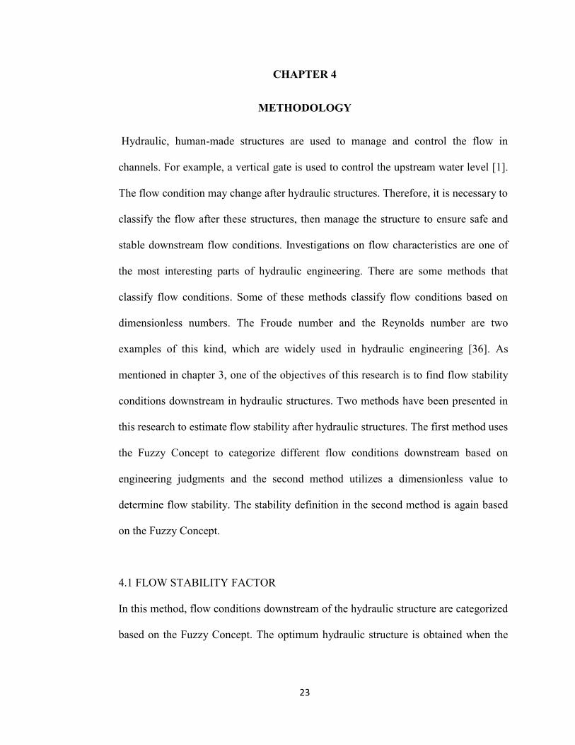
condition after hydraulic structures. Figures 4.1 (a to j) show the different flow
conditions after the hydraulic structures, which are determined based on engineering
judgment.
Table 4.1 Flow Stability Factor
Numbers Downstream condition Flow Stability Factor
1 Hydraulic Jump 0 2 Submerged Hydraulic Jump 0.2 3 Weak submerged H.J 0.4 4 Very weak submerged H.J 0.5 5 Strong wave 0.6 6 Wave 0.7 7 Weak wave
Weak Wave
0.8 8 Very weak wave 0.9 9 Stable 1
25
Figure 4.1. (a): Hydraulic jump at the end of the flume and far from the gate (St = 0)
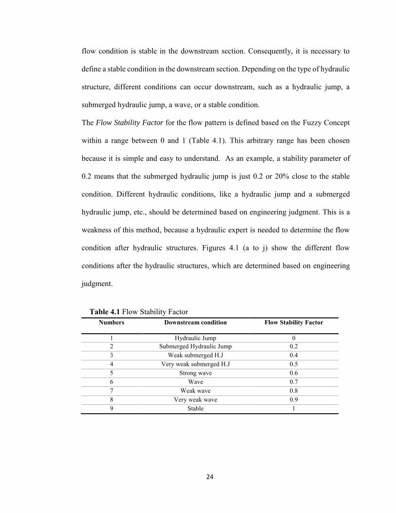
Figure 4.1. (b): Hydraulic jump after the gate (St = 0)
Figure 4.1. (c): Submerged hydraulic jump after the gate (St = 0.2)
26
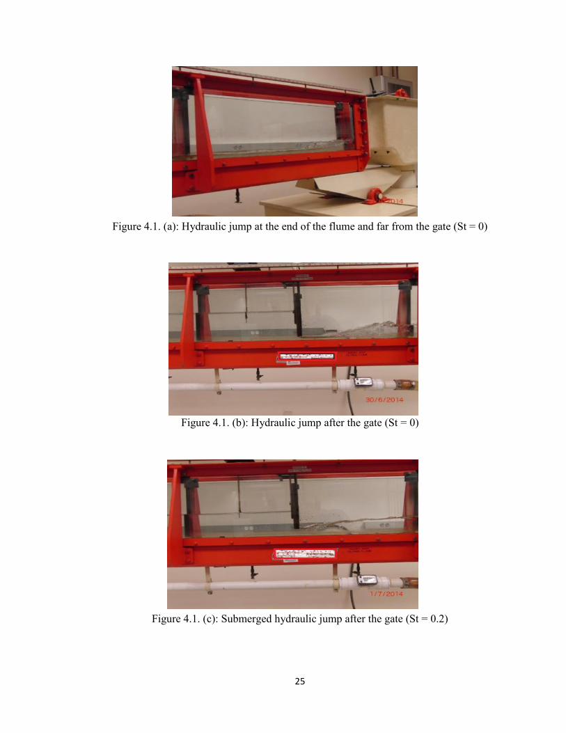
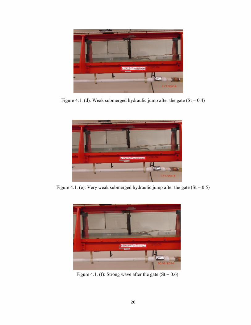
Figure 4.1. (d): Weak submerged hydraulic jump after the gate (St = 0.4)
Figure 4.1. (e): Very weak submerged hydraulic jump after the gate (St = 0.5)
Figure 4.1. (f): Strong wave after the gate (St = 0.6)
27
Figure 4.1. (g): Wave after the gate (St = 0.7)
Figure 4.1. (h): Weak wave after the gate (St = 0.8)
Figure 4.1. (i): Very weak wave after the gate (St = 0.9)
28
Figure 4.1. (j): Stable condition after the gate (St = 1)
4.2 FLOW STABILITY NUMBER
Unstable flow condition happens under some conditions. First, it occurs when the
velocity is high after the gated structures, resulting in erosion and sediment transport.
Second, it also happens when the depth of the flow is less than the critical depth and
the flow is supercritical. Third, it may occur when the flow is wavy. The change in the
energy of the flow along a structure can be used to investigate flow stability. The total
energy of the flow at a section includes bottom elevation, water depth, and the velocity
head in its definition; therefore, the total energy content and its change along a structure
is a good indicator of flow stability because it accounts for all the terms that relate to
flow instability. Flow instability primarily happens due to energy changes between two
sections along a stream, river, or channel. When the flow is “stable” in the first section,
then the flow will be “stable” again in the second section, if energy loss is negligible.
Regarding hydraulic behavior, a “stable” condition happens when the flow is sub-
critical in channels. Moreover, other factors, like surface flow fluctuations and bed and
wall velocities, are important to determine the acceptable flow stability range. Hamedi
29
and Fuentes [14] classified downstream flow conditions based on engineering
judgment to determine different flow conditions, like hydraulic jump, submerged
hydraulic jump, and wave, etc. This study introduces the Flow Stability Number and
the procedure to calculate this number. The study also considered other quantities (e.g.
hydraulic gradient, change in specific energy, and velocity head) as possible indicators
of flow stability; however, the change in total energy was selected given its full
accounting of the total energy at the sections of concern within the structure; in fact,
the change in total energy between sections within a structure is widely used in the
common design and operation of energy dissipation via hydraulic jumps, among other
structures
Two sections should be selected in the same flow direction; then, the energy of each
section is calculated and the two values are divided, that is the energy of the second
section is divided by the energy of the first section, thus determining the value of the
Flow Stability Number as a dimensionless number. The maximum value of the Flow
Stability Number is one. The Flow Stability Number is based on the Fuzzy Concept and
indicates the stability percentage of the flow in subcritical flows. For example, when
the Flow Stability Number is 0.67, it means that the flow is 67% stable. It should be
noted that both channel sections should be located after the hydraulic structure(s). The
first section should be selected immediately after the hydraulic structure(s) (in gates
after the vena-contracta) and the second section can be selected downstream of the first
section where the flow is uniform. Figure 4.2 shows the selected sections to calculate
energies after the vertical gate. In Figure 4.2 a, the jump is not submerged and the vena-
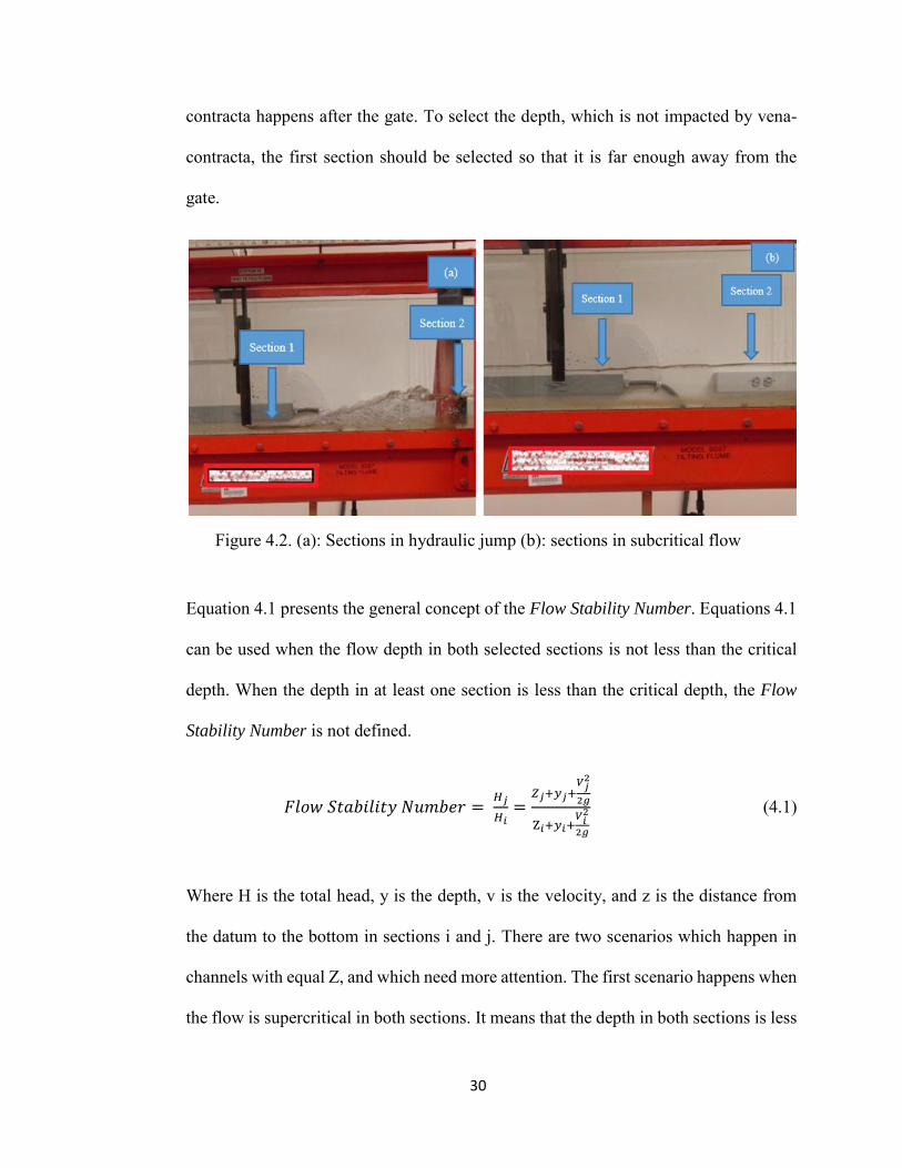
30
contracta happens after the gate. To select the depth, which is not impacted by vena-
contracta, the first section should be selected so that it is far enough away from the
gate.
Figure 4.2. (a): Sections in hydraulic jump (b): sections in subcritical flow
Equation 4.1 presents the general concept of the Flow Stability Number. Equations 4.1
can be used when the flow depth in both selected sections is not less than the critical
depth. When the depth in at least one section is less than the critical depth, the Flow
Stability Number is not defined.
𝐹𝑙𝑜𝑤 𝑆𝑡𝑎𝑏𝑖𝑙𝑖𝑡𝑦 𝑁𝑢𝑚𝑏𝑒𝑟 = 𝐻𝑗
𝐻𝑖=
𝑍𝑗+𝑦𝑗+𝑉𝑗
2
2𝑔
Z𝑖+𝑦𝑖+𝑉𝑖
2
2𝑔
(4.1)
Where H is the total head, y is the depth, v is the velocity, and z is the distance from
the datum to the bottom in sections i and j. There are two scenarios which happen in
channels with equal Z, and which need more attention. The first scenario happens when
the flow is supercritical in both sections. It means that the depth in both sections is less
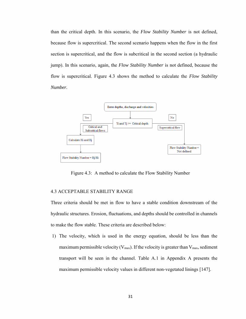
31
than the critical depth. In this scenario, the Flow Stability Number is not defined,
because flow is supercritical. The second scenario happens when the flow in the first
section is supercritical, and the flow is subcritical in the second section (a hydraulic
jump). In this scenario, again, the Flow Stability Number is not defined, because the
flow is supercritical. Figure 4.3 shows the method to calculate the Flow Stability
Number.
Figure 4.3: A method to calculate the Flow Stability Number
4.3 ACCEPTABLE STABILITY RANGE
Three criteria should be met in flow to have a stable condition downstream of the
hydraulic structures. Erosion, fluctuations, and depths should be controlled in channels
to make the flow stable. These criteria are described below:
1) The velocity, which is used in the energy equation, should be less than the
maximum permissible velocity (Vmax). If the velocity is greater than Vmax, sediment
transport will be seen in the channel. Table A.1 in Appendix A presents the
maximum permissible velocity values in different non-vegetated linings [147].
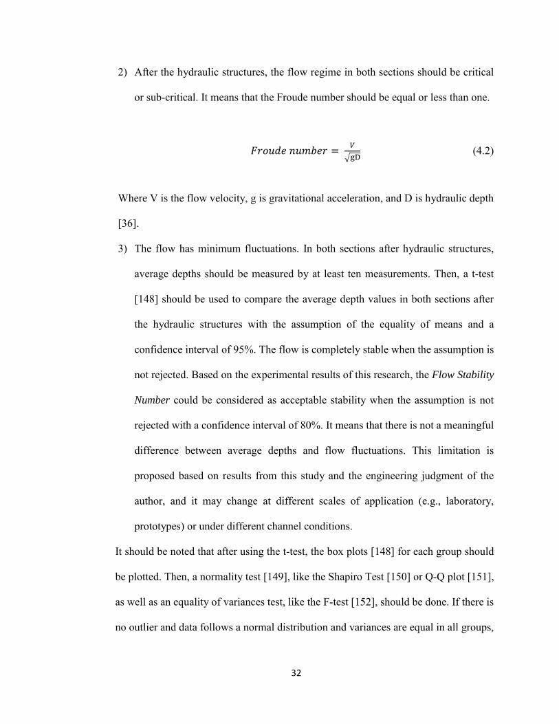
32
2) After the hydraulic structures, the flow regime in both sections should be critical
or sub-critical. It means that the Froude number should be equal or less than one.
𝐹𝑟𝑜𝑢𝑑𝑒 𝑛𝑢𝑚𝑏𝑒𝑟 = 𝑉
√gD (4.2)
Where V is the flow velocity, g is gravitational acceleration, and D is hydraulic depth
[36].
3) The flow has minimum fluctuations. In both sections after hydraulic structures,
average depths should be measured by at least ten measurements. Then, a t-test
[148] should be used to compare the average depth values in both sections after
the hydraulic structures with the assumption of the equality of means and a
confidence interval of 95%. The flow is completely stable when the assumption is
not rejected. Based on the experimental results of this research, the Flow Stability
Number could be considered as acceptable stability when the assumption is not
rejected with a confidence interval of 80%. It means that there is not a meaningful
difference between average depths and flow fluctuations. This limitation is
proposed based on results from this study and the engineering judgment of the
author, and it may change at different scales of application (e.g., laboratory,
prototypes) or under different channel conditions.
It should be noted that after using the t-test, the box plots [148] for each group should
be plotted. Then, a normality test [149], like the Shapiro Test [150] or Q-Q plot [151],
as well as an equality of variances test, like the F-test [152], should be done. If there is
no outlier and data follows a normal distribution and variances are equal in all groups,
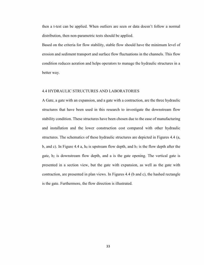
33
then a t-test can be applied. When outliers are seen or data doesn’t follow a normal
distribution, then non-parametric tests should be applied.
Based on the criteria for flow stability, stable flow should have the minimum level of
erosion and sediment transport and surface flow fluctuations in the channels. This flow
condition reduces aeration and helps operators to manage the hydraulic structures in a
better way.
4.4 HYDRAULIC STRUCTURES AND LABORATORIES
A Gate, a gate with an expansion, and a gate with a contraction, are the three hydraulic
structures that have been used in this research to investigate the downstream flow
stability condition. These structures have been chosen due to the ease of manufacturing
and installation and the lower construction cost compared with other hydraulic
structures. The schematics of these hydraulic structures are depicted in Figures 4.4 (a,
b, and c). In Figure 4.4 a, h0 is upstream flow depth, and h1 is the flow depth after the
gate, h2 is downstream flow depth, and a is the gate opening. The vertical gate is
presented in a section view, but the gate with expansion, as well as the gate with
contraction, are presented in plan views. In Figures 4.4 (b and c), the hashed rectangle
is the gate. Furthermore, the flow direction is illustrated.
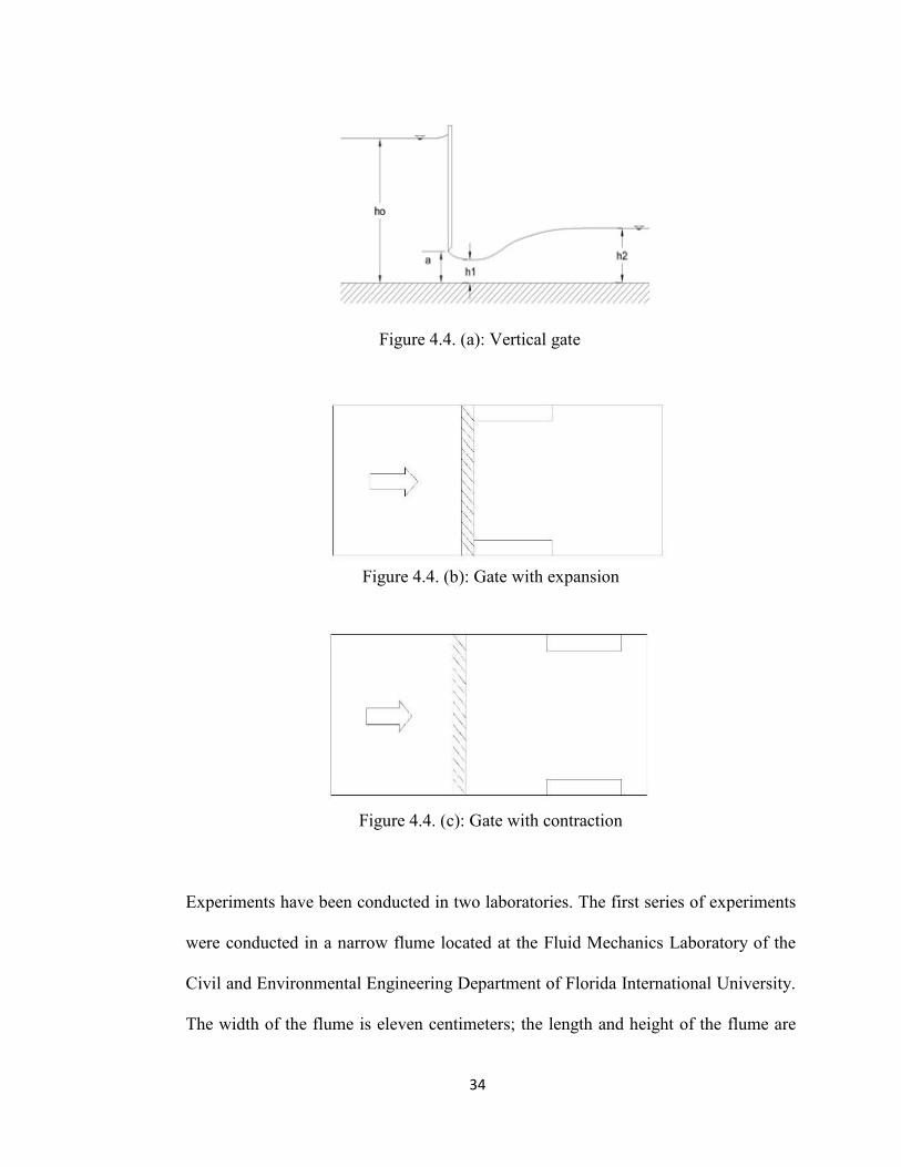
34
Figure 4.4. (a): Vertical gate
Figure 4.4. (b): Gate with expansion
Figure 4.4. (c): Gate with contraction
Experiments have been conducted in two laboratories. The first series of experiments
were conducted in a narrow flume located at the Fluid Mechanics Laboratory of the
Civil and Environmental Engineering Department of Florida International University.
The width of the flume is eleven centimeters; the length and height of the flume are
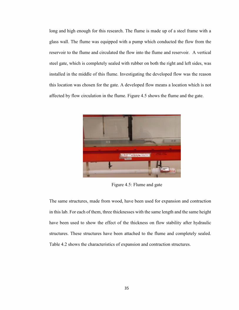
35
long and high enough for this research. The flume is made up of a steel frame with a
glass wall. The flume was equipped with a pump which conducted the flow from the
reservoir to the flume and circulated the flow into the flume and reservoir. A vertical
steel gate, which is completely sealed with rubber on both the right and left sides, was
installed in the middle of this flume. Investigating the developed flow was the reason
this location was chosen for the gate. A developed flow means a location which is not
affected by flow circulation in the flume. Figure 4.5 shows the flume and the gate.
The same structures, made from wood, have been used for expansion and contraction
in this lab. For each of them, three thicknesses with the same length and the same height
have been used to show the effect of the thickness on flow stability after hydraulic
structures. These structures have been attached to the flume and completely sealed.
Table 4.2 shows the characteristics of expansion and contraction structures.
Figure 4.5: Flume and gate
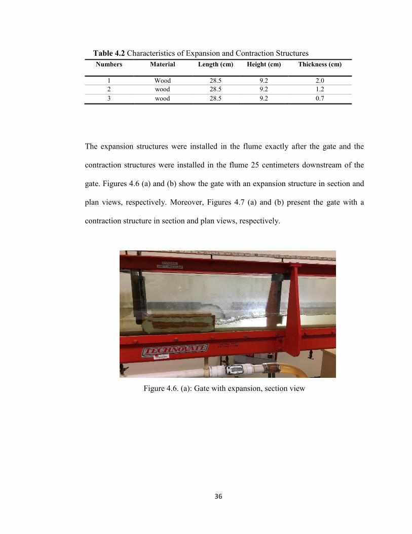
36
Table 4.2 Characteristics of Expansion and Contraction Structures Numbers Material Length (cm) Height (cm) Thickness (cm)
1 Wood 28.5 9.2 2.0 2 wood 28.5 9.2 1.2 3 wood 28.5 9.2 0.7
The expansion structures were installed in the flume exactly after the gate and the
contraction structures were installed in the flume 25 centimeters downstream of the
gate. Figures 4.6 (a) and (b) show the gate with an expansion structure in section and
plan views, respectively. Moreover, Figures 4.7 (a) and (b) present the gate with a
contraction structure in section and plan views, respectively.
Figure 4.6. (a): Gate with expansion, section view
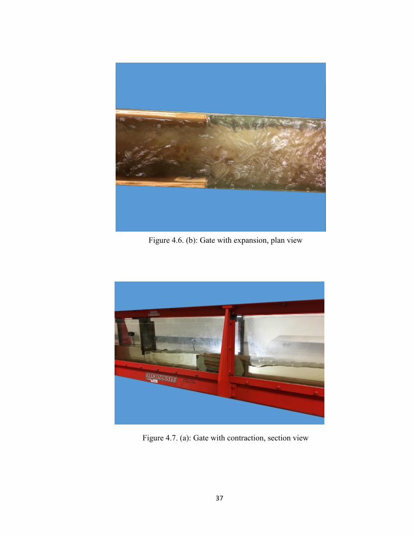
37
Figure 4.6. (b): Gate with expansion, plan view
Figure 4.7. (a): Gate with contraction, section view
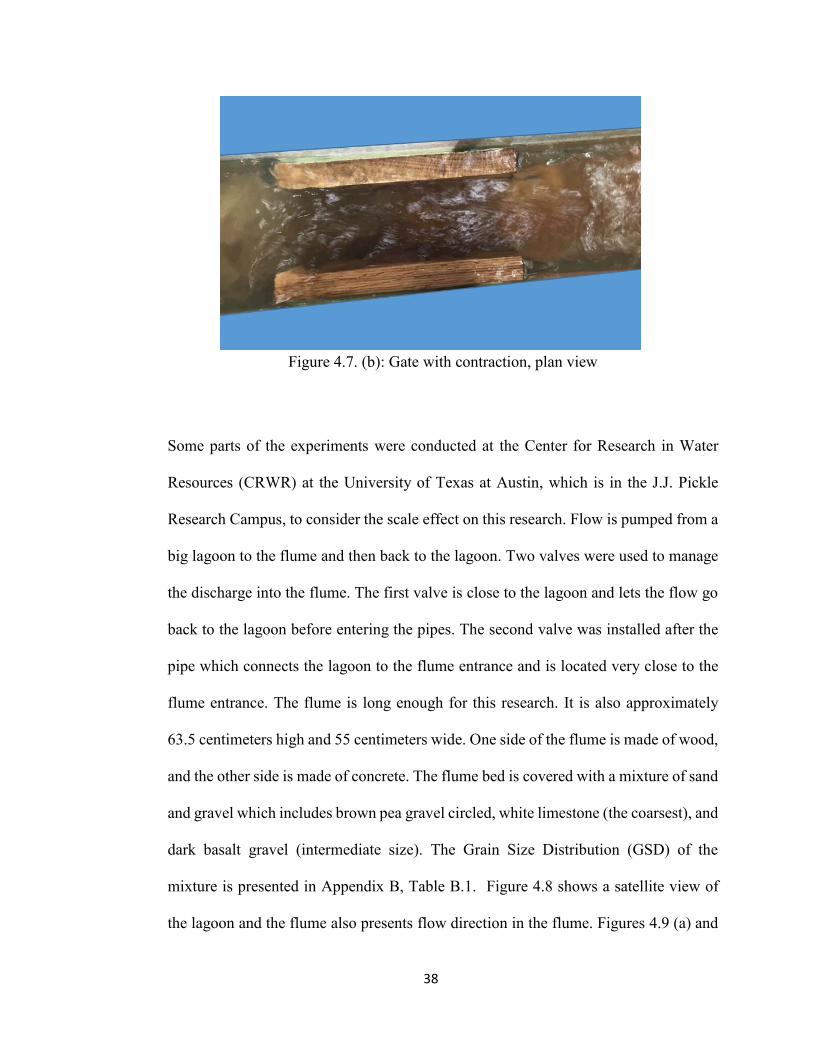
38
Figure 4.7. (b): Gate with contraction, plan view
Some parts of the experiments were conducted at the Center for Research in Water
Resources (CRWR) at the University of Texas at Austin, which is in the J.J. Pickle
Research Campus, to consider the scale effect on this research. Flow is pumped from a
big lagoon to the flume and then back to the lagoon. Two valves were used to manage
the discharge into the flume. The first valve is close to the lagoon and lets the flow go
back to the lagoon before entering the pipes. The second valve was installed after the
pipe which connects the lagoon to the flume entrance and is located very close to the
flume entrance. The flume is long enough for this research. It is also approximately
63.5 centimeters high and 55 centimeters wide. One side of the flume is made of wood,
and the other side is made of concrete. The flume bed is covered with a mixture of sand
and gravel which includes brown pea gravel circled, white limestone (the coarsest), and
dark basalt gravel (intermediate size). The Grain Size Distribution (GSD) of the
mixture is presented in Appendix B, Table B.1. Figure 4.8 shows a satellite view of
the lagoon and the flume also presents flow direction in the flume. Figures 4.9 (a) and
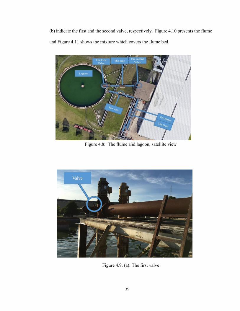
39
(b) indicate the first and the second valve, respectively. Figure 4.10 presents the flume
and Figure 4.11 shows the mixture which covers the flume bed.
Figure 4.8: The flume and lagoon, satellite view
Figure 4.9. (a): The first valve
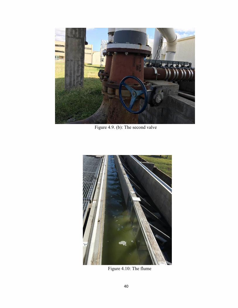
40
Figure 4.9. (b): The second valve
Figure 4.10: The flume

41
Figure 4.11: The mixture which covers the flume bed
The gate is made of wood with a steel frame. Two wooden parts were used in the gate;
the fixed part and the sliding part. The fixed part is 51 centimeters high and is thicker
than the sliding part to tolerate flow pressure and maintain the gate in a stable condition.
This part can be seen from downstream of the gate and is fixed with bar #10 at an
elevation of 78 centimeters from the bottom of the flume. The sliding part is 51
centimeters high and is less thick than the fixed portion. Because of its thickness, it
easily slides in the frame. This part can be seen from the upstream part of the gate. The
frame is fixed to both sides of the flume, and the gate slides up and down in the frame.
Therefore, the gate opening is easily managed. The sliding part of the gate is completely
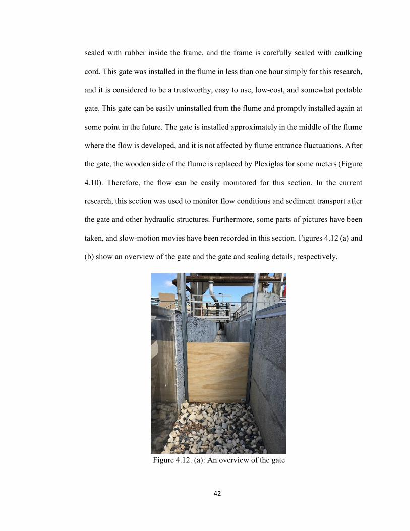
42
sealed with rubber inside the frame, and the frame is carefully sealed with caulking
cord. This gate was installed in the flume in less than one hour simply for this research,
and it is considered to be a trustworthy, easy to use, low-cost, and somewhat portable
gate. This gate can be easily uninstalled from the flume and promptly installed again at
some point in the future. The gate is installed approximately in the middle of the flume
where the flow is developed, and it is not affected by flume entrance fluctuations. After
the gate, the wooden side of the flume is replaced by Plexiglas for some meters (Figure
4.10). Therefore, the flow can be easily monitored for this section. In the current
research, this section was used to monitor flow conditions and sediment transport after
the gate and other hydraulic structures. Furthermore, some parts of pictures have been
taken, and slow-motion movies have been recorded in this section. Figures 4.12 (a) and
(b) show an overview of the gate and the gate and sealing details, respectively.
Figure 4.12. (a): An overview of the gate
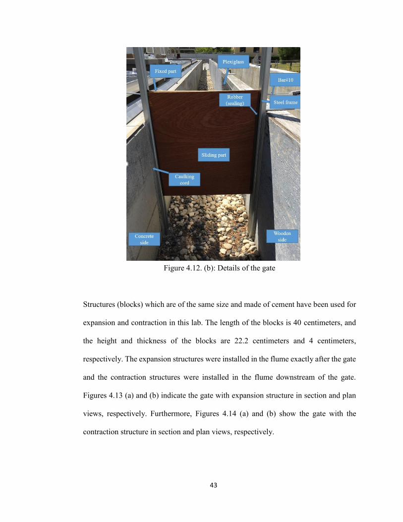
43
Figure 4.12. (b): Details of the gate
Structures (blocks) which are of the same size and made of cement have been used for
expansion and contraction in this lab. The length of the blocks is 40 centimeters, and
the height and thickness of the blocks are 22.2 centimeters and 4 centimeters,
respectively. The expansion structures were installed in the flume exactly after the gate
and the contraction structures were installed in the flume downstream of the gate.
Figures 4.13 (a) and (b) indicate the gate with expansion structure in section and plan
views, respectively. Furthermore, Figures 4.14 (a) and (b) show the gate with the
contraction structure in section and plan views, respectively.
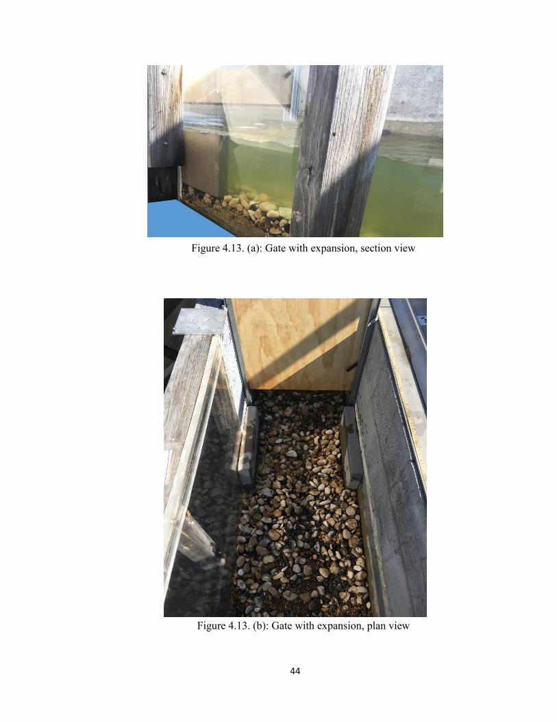
44
Figure 4.13. (a): Gate with expansion, section view
Figure 4.13. (b): Gate with expansion, plan view
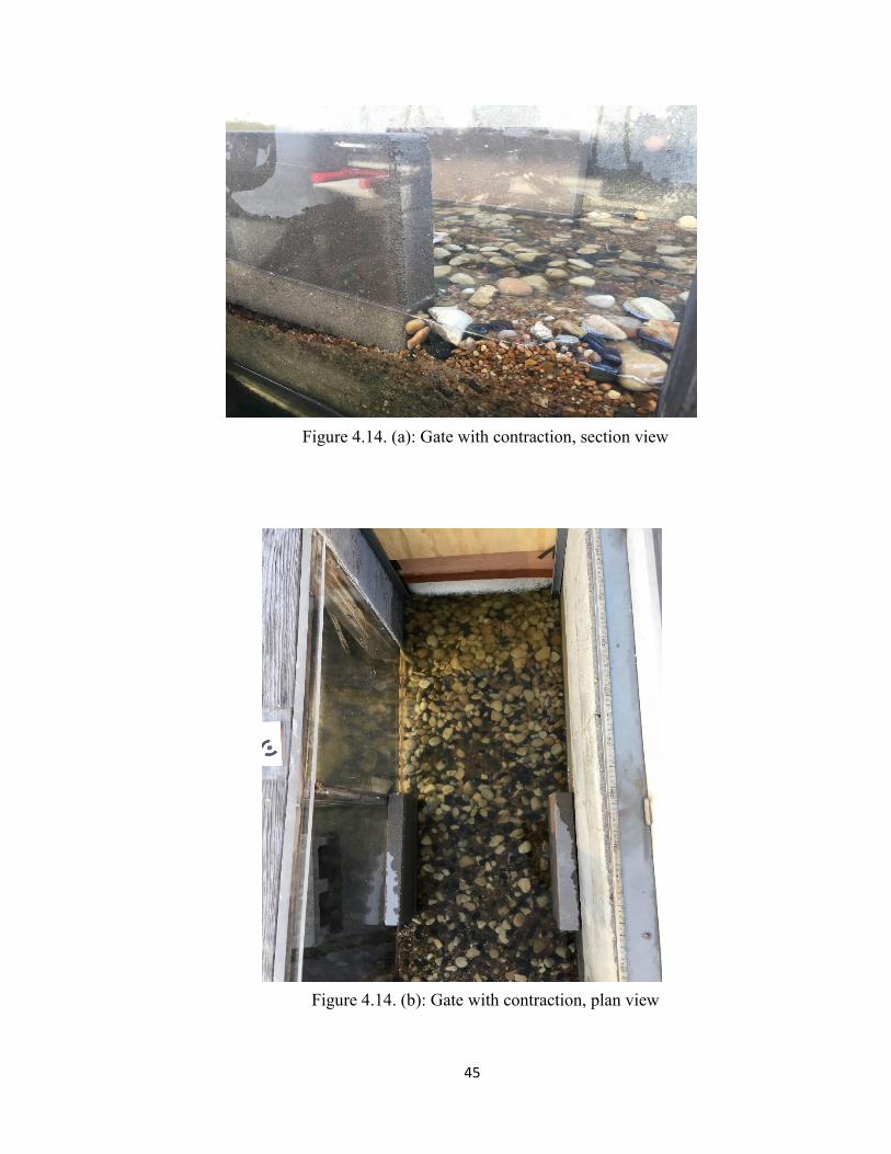
45
Figure 4.14. (a): Gate with contraction, section view
Figure 4.14. (b): Gate with contraction, plan view
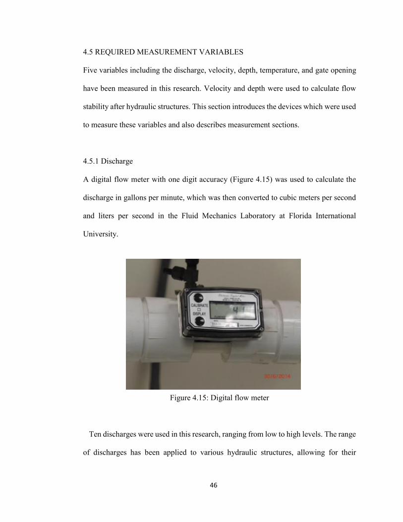
46
4.5 REQUIRED MEASUREMENT VARIABLES
Five variables including the discharge, velocity, depth, temperature, and gate opening
have been measured in this research. Velocity and depth were used to calculate flow
stability after hydraulic structures. This section introduces the devices which were used
to measure these variables and also describes measurement sections.
4.5.1 Discharge
A digital flow meter with one digit accuracy (Figure 4.15) was used to calculate the
discharge in gallons per minute, which was then converted to cubic meters per second
and liters per second in the Fluid Mechanics Laboratory at Florida International
University.
Figure 4.15: Digital flow meter
Ten discharges were used in this research, ranging from low to high levels. The range
of discharges has been applied to various hydraulic structures, allowing for their
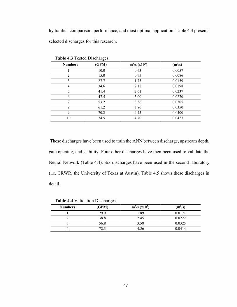
47
hydraulic comparison, performance, and most optimal application. Table 4.3 presents
selected discharges for this research.
Table 4.3 Tested Discharges
Numbers (GPM)
(GPM)
m3/s (x103) (m2/s) 1 10.0 0.63 0.0057
2 15.0 0.95 0.0086 3 27.7 1.75 0.0159 4 34.6 2.18 0.0198 5 41.4 2.61 0.0237 6 47.5 3.00 0.0270 7 53.2 3.36 0.0305 8 61.2 3.86 0.0350 9 70.2 4.43 0.0400 10 74.5 4.70 0.0427
These discharges have been used to train the ANN between discharge, upstream depth,
gate opening, and stability. Four other discharges have then been used to validate the
Neural Network (Table 4.4). Six discharges have been used in the second laboratory
(i.e. CRWR, the University of Texas at Austin). Table 4.5 shows these discharges in
detail.
Table 4.4 Validation Discharges
Numbers (GPM)
m3/s (x103) (m2/s) 1 29.9 1.89 0.0171 2 38.8 2.45 0.0222 3 56.8 3.58 0.0325 4 72.3 4.56 0.0414
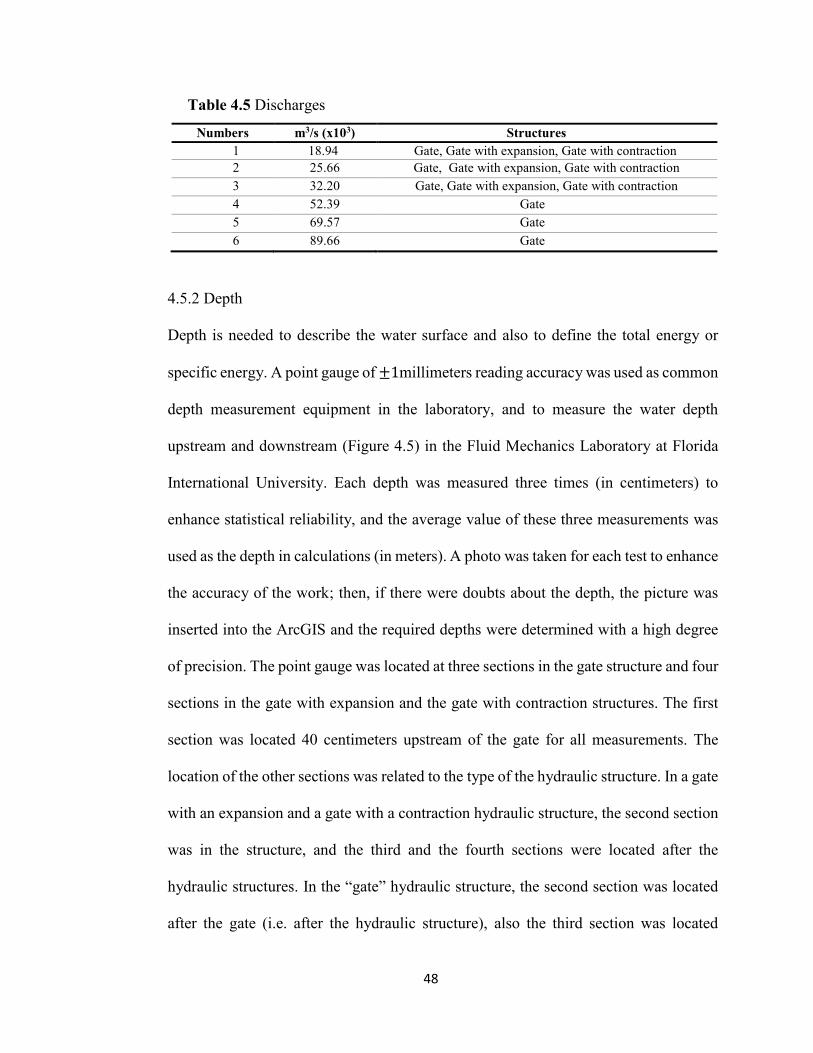
48
Table 4.5 Discharges
4.5.2 Depth
Depth is needed to describe the water surface and also to define the total energy or
specific energy. A point gauge of ±1millimeters reading accuracy was used as common
depth measurement equipment in the laboratory, and to measure the water depth
upstream and downstream (Figure 4.5) in the Fluid Mechanics Laboratory at Florida
International University. Each depth was measured three times (in centimeters) to
enhance statistical reliability, and the average value of these three measurements was
used as the depth in calculations (in meters). A photo was taken for each test to enhance
the accuracy of the work; then, if there were doubts about the depth, the picture was
inserted into the ArcGIS and the required depths were determined with a high degree
of precision. The point gauge was located at three sections in the gate structure and four
sections in the gate with expansion and the gate with contraction structures. The first
section was located 40 centimeters upstream of the gate for all measurements. The
location of the other sections was related to the type of the hydraulic structure. In a gate
with an expansion and a gate with a contraction hydraulic structure, the second section
was in the structure, and the third and the fourth sections were located after the
hydraulic structures. In the “gate” hydraulic structure, the second section was located
after the gate (i.e. after the hydraulic structure), also the third section was located
Numbers m3/s (x103) Structures 1 18.94 Gate, Gate with expansion, Gate with contraction 2 25.66 Gate, Gate with expansion, Gate with contraction 3 32.20 Gate, Gate with expansion, Gate with contraction 4 52.39 Gate 5 69.57 Gate 6 89.66 Gate
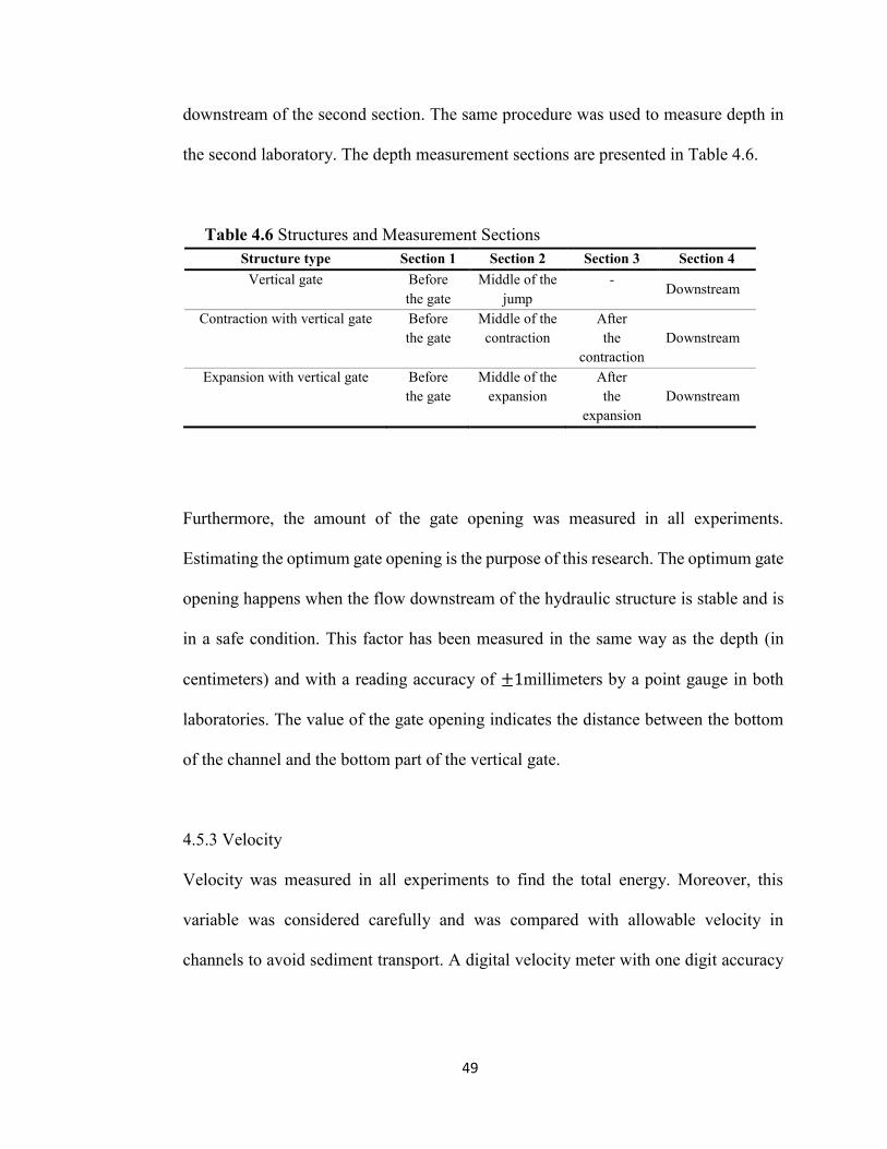
49
downstream of the second section. The same procedure was used to measure depth in
the second laboratory. The depth measurement sections are presented in Table 4.6.
Table 4.6 Structures and Measurement Sections Structure type Section 1 Section 2 Section 3 Section 4
Vertical gate Before the gate
Middle of the jump
- Downstream
Contraction with vertical gate Before the gate
Middle of the contraction
After the
contraction Downstream
Expansion with vertical gate Before the gate
Middle of the expansion
After the
expansion Downstream
Furthermore, the amount of the gate opening was measured in all experiments.
Estimating the optimum gate opening is the purpose of this research. The optimum gate
opening happens when the flow downstream of the hydraulic structure is stable and is
in a safe condition. This factor has been measured in the same way as the depth (in
centimeters) and with a reading accuracy of ±1millimeters by a point gauge in both
laboratories. The value of the gate opening indicates the distance between the bottom
of the channel and the bottom part of the vertical gate.
4.5.3 Velocity
Velocity was measured in all experiments to find the total energy. Moreover, this
variable was considered carefully and was compared with allowable velocity in
channels to avoid sediment transport. A digital velocity meter with one digit accuracy

50
was used in this research to determine the velocity in meters per second (both
laboratories). Figure 4.16 shows the digital velocity meter.
Figure 4.16: Digital velocity meter (globalindustrial.com)
The sections which were used to measure depth were also used to determine velocity
(Table 4.6). Velocity was measured using two methods. When the depth was deep (high
discharge), the velocity was measured at 0.2 and 0.8 depth from the surface and the
average of these two values was used as velocity. On the other hand, when the depth
was not deep enough, the velocity was only measured at 0.6 depth from the surface.
All measurements were repeated three times to reduce the error and the average of these
three measurements were used as velocity in the calculations.
4.5.4 Temperature
The Reynolds number is affected by temperature; therefore, this variable was measured
in all the experiments. A digital thermometer with one digit accuracy was used in the
51
first laboratory (FIU) to measure the temperature in Celsius (oC). The thermometer is
presented in Figure 4.17. In the second laboratory (CRWR – UT Austin), the velocity
meter (Figure 2.16) was used to measure the temperature with one digit accuracy, again
in Celsius (oC). This device can measure temperature as well as velocity. The sections
which were used to measure depth were also used to determine the temperature in both
laboratories (Table 4.6).
Figure 4.17: Digital thermometer (homedepot.com)
4.5.5 Flow Pattern
The flow pattern is one of the most important factors in determining the downstream
flow stability of the hydraulic structures based on both definitions previously presented
in this chapter. Pictures and movies were captured and recorded by a high-speed camera
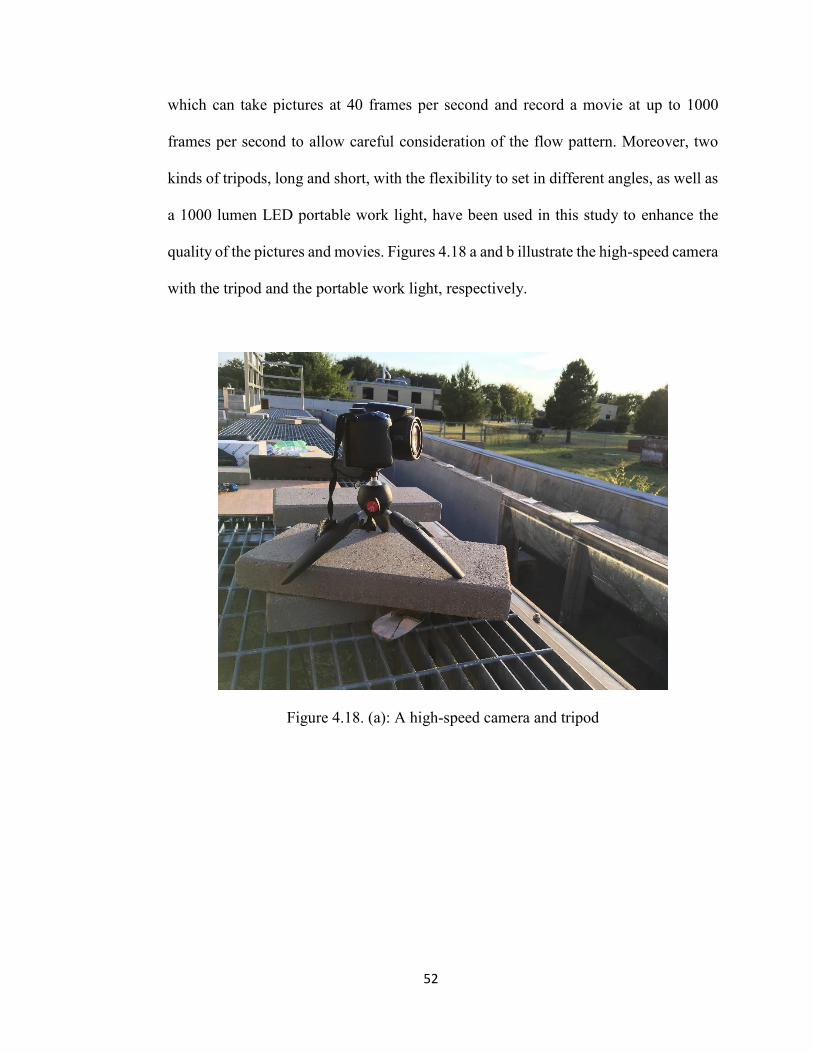
52
which can take pictures at 40 frames per second and record a movie at up to 1000
frames per second to allow careful consideration of the flow pattern. Moreover, two
kinds of tripods, long and short, with the flexibility to set in different angles, as well as
a 1000 lumen LED portable work light, have been used in this study to enhance the
quality of the pictures and movies. Figures 4.18 a and b illustrate the high-speed camera
with the tripod and the portable work light, respectively.
Figure 4.18. (a): A high-speed camera and tripod
53
Figure 4.18. (b): 1000 lumen LED portable work light (homedepot.com)
4.6 ARTIFICIAL INTELLIGENCE METHODS
Two artificial intelligence methods, the Fuzzy Concept and the Artificial Neural
Network (ANN), have been used in this study to define the stability concept and predict
the amount of the gate opening.
4.6.1 The Fuzzy Concept
The Fuzzy Concept has been used to define flow stability types (flow categories)
downstream of the vertical gates in sections 4.1 and 4.2. When the flow experienced a
hydraulic jump that means that the flow is completely unstable and the stability number
is not defined in supercritical flow. On the other hand, when the flow is sub- critical
and the velocity is low, the flow is completely stable (100%) and the assigned stability
54
number for this type of flow is “1.” Between these two flow types, there are some other
types of flow with an assigned stability number of more than zero and less than one.
This concept is borrowed from the Fuzzy Concept, which was introduced by Zadeh
[153].
4.6.2 Artificial Neural Network (ANN)
In this research, the Artificial Neural Network toolbox in MATLAB was used to predict
the amount of the gate opening. The stability parameter and the unit discharge are
imported as inputs and the upstream depth over the gate opening is calculated as output
using Multi-Layer Perceptron (MLP) in ANN. Two layers with ten neurons in each
layer were used to create the network. This method, however, does not result in very
accurate results when there is not a lot of data, and it needs some corrections to reduce
error. Therefore, a regression-based post-processing method has been introduced and
applied in this study to reduce error. The results indicate that the post-processing
method effectively works when fewer data points are available. Various statistical
methods (e.g., RMSE and Nash-Sutcliff) have been used to determine model accuracy.
The details of the ANN network and the post-possessing method which were used are
presented in the results and discussion chapter.
4.7 DIMENSIONLESS PARAMETERS
The first step in calculating the optimum hydraulic structure is determining all relevant
dimensionless parameters. The Buckingham Pi Theorem has been used to find effective
dimensionless parameters. Some parameters like density, gravitational acceleration,
55
upstream depth, critical depth, gate opening, viscosity, downstream depth, and slope
are important to develop the most effective dimensionless parameters. For each
hydraulic structure, the set of dimensionless parameters has been determined and used
in graphs, calculations, and relationships. These sets of dimensionless parameters are
introduced and described in their specific sections in the results and discussion chapter.
Moreover, two dimensionless numbers are important in this research. The Froude
number and the Reynolds number. The Froude number is a ratio of inertia force to
gravity force and the Reynolds number is a ratio of inertia force to viscosity force.
𝐹𝑟2 = 𝐼𝑛𝑒𝑟𝑡𝑖𝑎 𝑓𝑜𝑟𝑐𝑒
𝐺𝑒𝑟𝑎𝑣𝑖𝑡𝑦 𝑓𝑜𝑟𝑐𝑒=
𝑚𝑎𝑠𝑠 × 𝑎𝑐𝑐𝑒𝑙𝑒𝑟𝑎𝑡𝑖𝑜𝑛
𝑚𝑎𝑠𝑠 × 𝑔𝑟𝑎𝑣𝑖𝑡𝑦 𝑎𝑐𝑐𝑒𝑙𝑒𝑟𝑎𝑡𝑖𝑜𝑛
=
𝑣𝑒𝑙𝑜𝑐𝑖𝑡𝑦𝑡𝑖𝑚𝑒
𝑔𝑟𝑎𝑣𝑖𝑡𝑦 𝑎𝑐𝑐𝑒𝑙𝑒𝑟𝑎𝑡𝑖𝑜𝑛
(𝑉𝑡
)
𝑔=
𝑉
𝑡𝑔=
𝑉
𝐷𝑉 × 𝑔
= 𝑉2
𝐷𝑔 → 𝐹𝑟 =
𝑉
√𝑔𝐷 (4.3)
𝑅𝑒 = 𝐼𝑛𝑒𝑟𝑡𝑖𝑎 𝑓𝑜𝑟𝑐𝑒
𝑉𝑖𝑠𝑐𝑜𝑠𝑖𝑡𝑦 𝑓𝑜𝑟𝑐𝑒=
𝑚𝑎𝑠𝑠 × 𝑎𝑐𝑐𝑒𝑙𝑒𝑟𝑎𝑡𝑖𝑜𝑛
𝑠ℎ𝑒𝑎𝑟 𝑠𝑡𝑟𝑒𝑠𝑠 × 𝑎𝑟𝑒𝑎
= 𝑣𝑜𝑙𝑢𝑚𝑒 × 𝑑𝑒𝑛𝑠𝑖𝑡𝑦 ×
𝑣𝑒𝑙𝑜𝑐𝑖𝑡𝑦𝑡𝑖𝑚𝑒
𝑠ℎ𝑒𝑎𝑟 𝑠𝑡𝑟𝑒𝑠𝑠 × 𝑎𝑟𝑒𝑎
𝑣𝑜𝑙𝑢𝑚𝑒
𝑡𝑖𝑚𝑒 ×𝑑𝑒𝑛𝑠𝑖𝑡𝑦 ×𝑣𝑒𝑙𝑜𝑐𝑖𝑡𝑦
𝑠ℎ𝑒𝑎𝑟 𝑠𝑡𝑟𝑒𝑠𝑠 ×𝑎𝑟𝑒𝑎=
𝑎𝑟𝑒𝑎 ×𝑣𝑒𝑙𝑜𝑐𝑖𝑡𝑦 ×𝑑𝑒𝑛𝑠𝑖𝑡𝑦 ×𝑣𝑒𝑙𝑜𝑐𝑖𝑡𝑦
𝑠ℎ𝑒𝑎𝑟 𝑠𝑡𝑟𝑒𝑠𝑠 ×𝑎𝑟𝑒𝑎
𝑣𝑒𝑙𝑜𝑐𝑖𝑡𝑦 × 𝑑𝑒𝑛𝑠𝑖𝑡𝑦 × 𝑣𝑒𝑙𝑜𝑐𝑖𝑡𝑦
𝑠ℎ𝑒𝑎𝑟 𝑠𝑡𝑟𝑒𝑠𝑠=
𝑉𝜌𝑉
𝜇 (𝑑𝑉𝑑𝑦
)=
𝑉𝜌𝑉
𝜇𝑉𝐿
= 𝑉𝜌𝜇𝐿
= 𝑉𝐿𝜇𝜌
(4.4)
56
CHAPTER 5
RESULTS & DISCUSSION
SECTION 1
OPTIMIZING GATE OPENINGS FOR FLOW REGIME CONTROL:
EXPERIMENTAL AND ARTIFICIAL NEURAL NETWORK
DEVELOPEMENT
Vertical gates are important structures that control flow characteristics in both
downstream and upstream flows in streams and canals. In this investigation, laboratory
tests were conducted to find the optimum vertical gate opening as a function of the
upstream water level to yield a stable downstream condition. Physical simulations were
conducted within a range of discharges for the experimental flume. Fuzzy Concepts
were also used to define the Flow Stability Factor. Experimental results were then
analyzed via an artificial neural network (ANN) to estimate the optimum gate opening.
The ANN results were post-processed via regression analysis to minimize estimation
errors. This investigation highlights the potential for optimizing hydraulic performance
based on regression-based post-processing ANN to define optimal design, analysis, and
operating conditions for hydraulic structures (e.g., gates) in controlling stream flow
conditions.
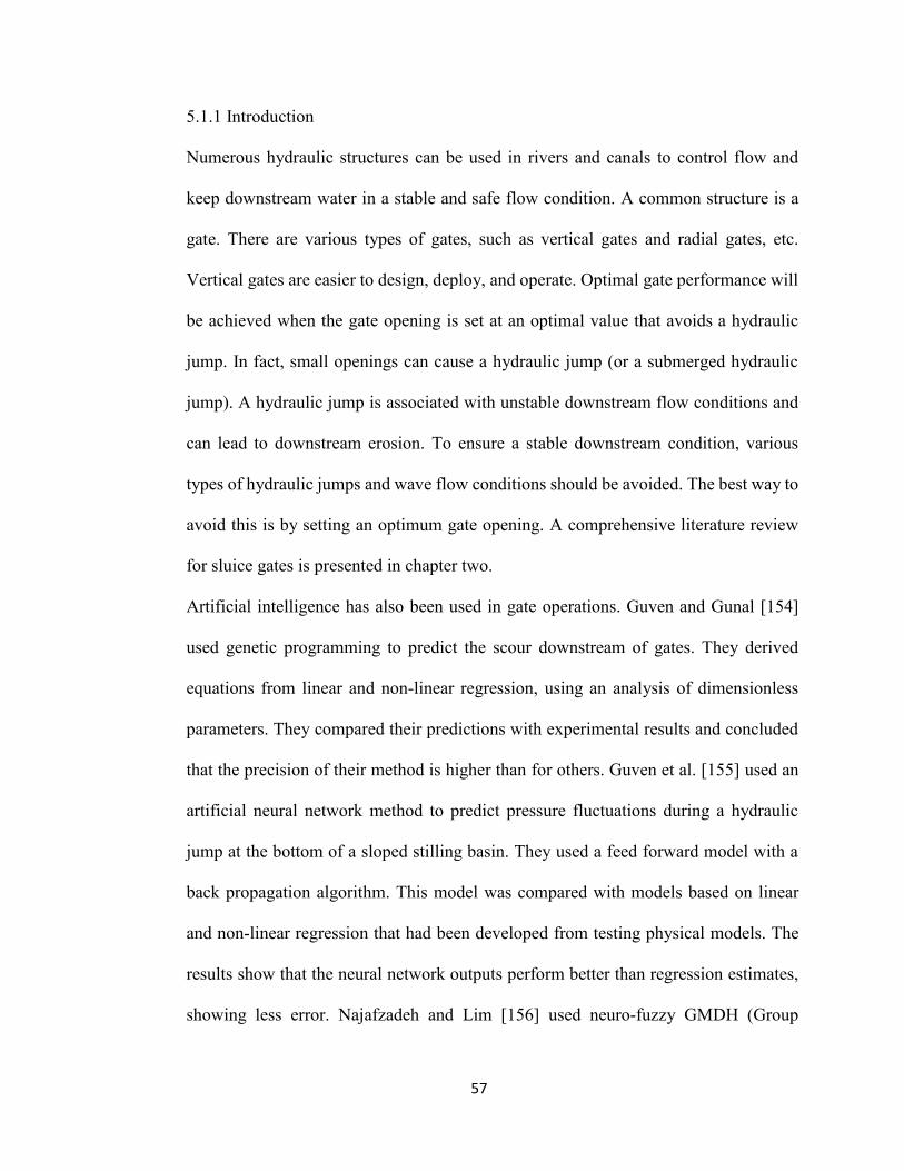
57
5.1.1 Introduction
Numerous hydraulic structures can be used in rivers and canals to control flow and
keep downstream water in a stable and safe flow condition. A common structure is a
gate. There are various types of gates, such as vertical gates and radial gates, etc.
Vertical gates are easier to design, deploy, and operate. Optimal gate performance will
be achieved when the gate opening is set at an optimal value that avoids a hydraulic
jump. In fact, small openings can cause a hydraulic jump (or a submerged hydraulic
jump). A hydraulic jump is associated with unstable downstream flow conditions and
can lead to downstream erosion. To ensure a stable downstream condition, various
types of hydraulic jumps and wave flow conditions should be avoided. The best way to
avoid this is by setting an optimum gate opening. A comprehensive literature review
for sluice gates is presented in chapter two.
Artificial intelligence has also been used in gate operations. Guven and Gunal [154]
used genetic programming to predict the scour downstream of gates. They derived
equations from linear and non-linear regression, using an analysis of dimensionless
parameters. They compared their predictions with experimental results and concluded
that the precision of their method is higher than for others. Guven et al. [155] used an
artificial neural network method to predict pressure fluctuations during a hydraulic
jump at the bottom of a sloped stilling basin. They used a feed forward model with a
back propagation algorithm. This model was compared with models based on linear
and non-linear regression that had been developed from testing physical models. The
results show that the neural network outputs perform better than regression estimates,
showing less error. Najafzadeh and Lim [156] used neuro-fuzzy GMDH (Group
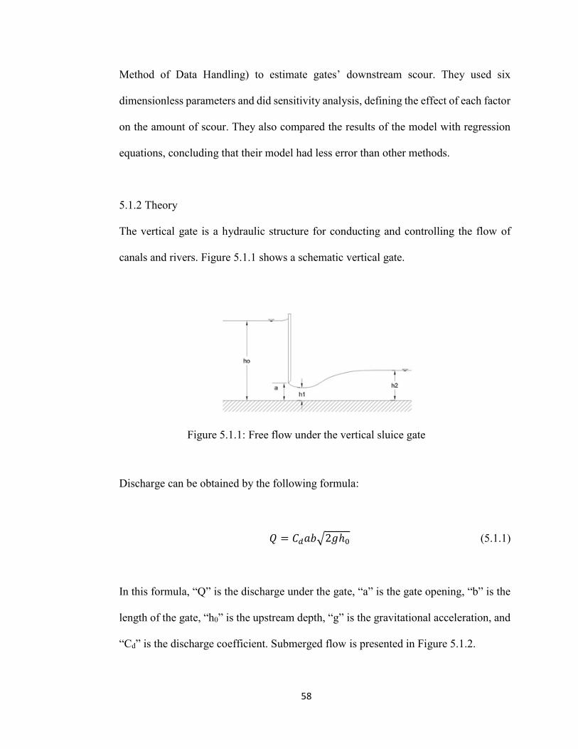
58
Method of Data Handling) to estimate gates’ downstream scour. They used six
dimensionless parameters and did sensitivity analysis, defining the effect of each factor
on the amount of scour. They also compared the results of the model with regression
equations, concluding that their model had less error than other methods.
5.1.2 Theory
The vertical gate is a hydraulic structure for conducting and controlling the flow of
canals and rivers. Figure 5.1.1 shows a schematic vertical gate.
Figure 5.1.1: Free flow under the vertical sluice gate
Discharge can be obtained by the following formula:
𝑄 = 𝐶𝑑𝑎𝑏√2𝑔ℎ0 (5.1.1)
In this formula, “Q” is the discharge under the gate, “a” is the gate opening, “b” is the
length of the gate, “h0” is the upstream depth, “g” is the gravitational acceleration, and
“Cd” is the discharge coefficient. Submerged flow is presented in Figure 5.1.2.
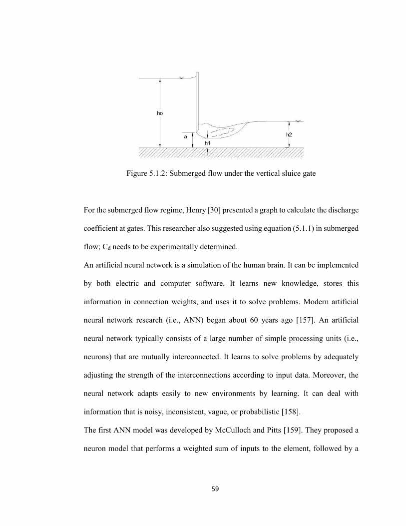
59
Figure 5.1.2: Submerged flow under the vertical sluice gate
For the submerged flow regime, Henry [30] presented a graph to calculate the discharge
coefficient at gates. This researcher also suggested using equation (5.1.1) in submerged
flow; Cd needs to be experimentally determined.
An artificial neural network is a simulation of the human brain. It can be implemented
by both electric and computer software. It learns new knowledge, stores this
information in connection weights, and uses it to solve problems. Modern artificial
neural network research (i.e., ANN) began about 60 years ago [157]. An artificial
neural network typically consists of a large number of simple processing units (i.e.,
neurons) that are mutually interconnected. It learns to solve problems by adequately
adjusting the strength of the interconnections according to input data. Moreover, the
neural network adapts easily to new environments by learning. It can deal with
information that is noisy, inconsistent, vague, or probabilistic [158].
The first ANN model was developed by McCulloch and Pitts [159]. They proposed a
neuron model that performs a weighted sum of inputs to the element, followed by a
60
threshold logical operation. Hebb [160] proposed a learning scheme for adjusting a
connection weight based on pre- and post-synaptic variable values. Minsky [161]
developed a learning machine in which the connection strength could be automatically
adapted. Rosenblatt [162] proposed that a perception model that has adjustable weights
be the perception learning law. Minsky and Papert [163] produced a multilayer
perceptron (MLP) to solve difficult problems. Hopfield [164] developed an energy
analysis for feedback neural networks.
The MLP is made up of elements or perceptrons that are based on the McCulloch and
Pitts [159] model of a simple human neural. The perceptron units are made up of
multiple inputs linked via weighted connections (synapses or weights) to summing and
nonlinear squashing functions. When perceptrons are connected in a network with more
than one layer, the subsequent structure is called an MLP (Figure 5.1.3).
MLPs, with the correct weight configurations, can be used to solve many problems in
pattern recognition, system identification, and time series prediction. The strength of
the MLP is that the underlying rules of the function do not need to be known prior to
network training (i.e., finding the relationship between inputs and outputs in a black
box). During the training process, assuming there is a representative training data set,
the network extracts the mapping function in its internal representation, thus obtaining
a solution. The simplicity of this solution adds to its usefulness. It is important to note,
however, that in some applications it is necessary to know how the task has been solved.
The black-box nature of the MLP can be a drawback rather than a strength [165].
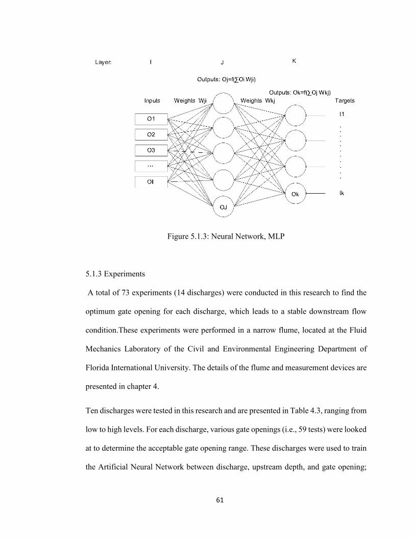
61
Figure 5.1.3: Neural Network, MLP
5.1.3 Experiments
A total of 73 experiments (14 discharges) were conducted in this research to find the
optimum gate opening for each discharge, which leads to a stable downstream flow
condition.These experiments were performed in a narrow flume, located at the Fluid
Mechanics Laboratory of the Civil and Environmental Engineering Department of
Florida International University. The details of the flume and measurement devices are
presented in chapter 4.
Ten discharges were tested in this research and are presented in Table 4.3, ranging from
low to high levels. For each discharge, various gate openings (i.e., 59 tests) were looked
at to determine the acceptable gate opening range. These discharges were used to train
the Artificial Neural Network between discharge, upstream depth, and gate opening;
62
then, four other discharges (i.e., 14 tests) were used to validate the Neural Network
(Table 4.4).
Finding the optimum gate opening for each upstream depth and discharge is the purpose
of this research. The optimum gate opening is obtained when the flow condition is
stable in the downstream section, and consequently, it is necessary to define a stable
condition in the downstream section. Depending on the gate opening, different
conditions can occur downstream, such as a hydraulic jump, a submerged hydraulic
jump, a wave, or a stable condition.
The Flow Stability Factor is defined in chapter 4, based on the Fuzzy Concept, to
classify the downstream flow condition and consequently determine the optimum gate
opening (Table 4.1).
For each discharge, various gate openings were examined. For each gate opening, the
downstream flow condition was recorded. The first step in calculating the optimum
gate opening is to determine all relevant dimensionless parameters.
Unit discharges and dimensionless parameters were applied in this study; therefore, the
results can be used in real streams and rivers. However, a scale effect should be taken
into account to validate the results or to find a correction factor for the outcomes due
to the small dimensions used in this research. Roth and Hager [1] noted that due to fluid
viscosity, channel width has an effect on the minimum gate opening. They stated that
for any channel width and with inviscid flow, for the Froude similarity to apply, a gate
opening of at least approximately 50 millimeters is required. Also, they reported that
narrower channels need a higher minimum gate opening. The flume which was used in
this research was narrow (11 centimeters), and some gate openings were less than the

63
minimum gate opening reported by Roth and Hager [1]. It should be noted that Roth
and Hager’s claim is based on fluid viscosity which can vary with temperature and
water quality. The flow classification which is used in this research can be applied in
larger scale models.
5.1.4 Neural Network
The neural network toolbox (i.e., nntool) in Matlab was used to create a network for
predicting the optimum gate opening. The critical depth and upstream depth are
network inputs, and “a” is the network output. First, stable conditions were separated
from all the tests. A network was then generated for eight critical depths, and four other
critical depths were used to validate the network. The characteristics of the neural
network are as follows:
Multi-layer perceptron (MLP);
Inputs: unit discharge and Flow Stability Factor;
Target: h0/a;
Network type: Feed-forward backprop;
Training function: TRAINLM;
Adaption learning function: LEARNGDM;
Performance function: MSE;
Number of layers: 2;
Property for the first layer: 10 Neurons;
Property for the second layer: 10 Neurons; and
Transfer function: PURELIN.
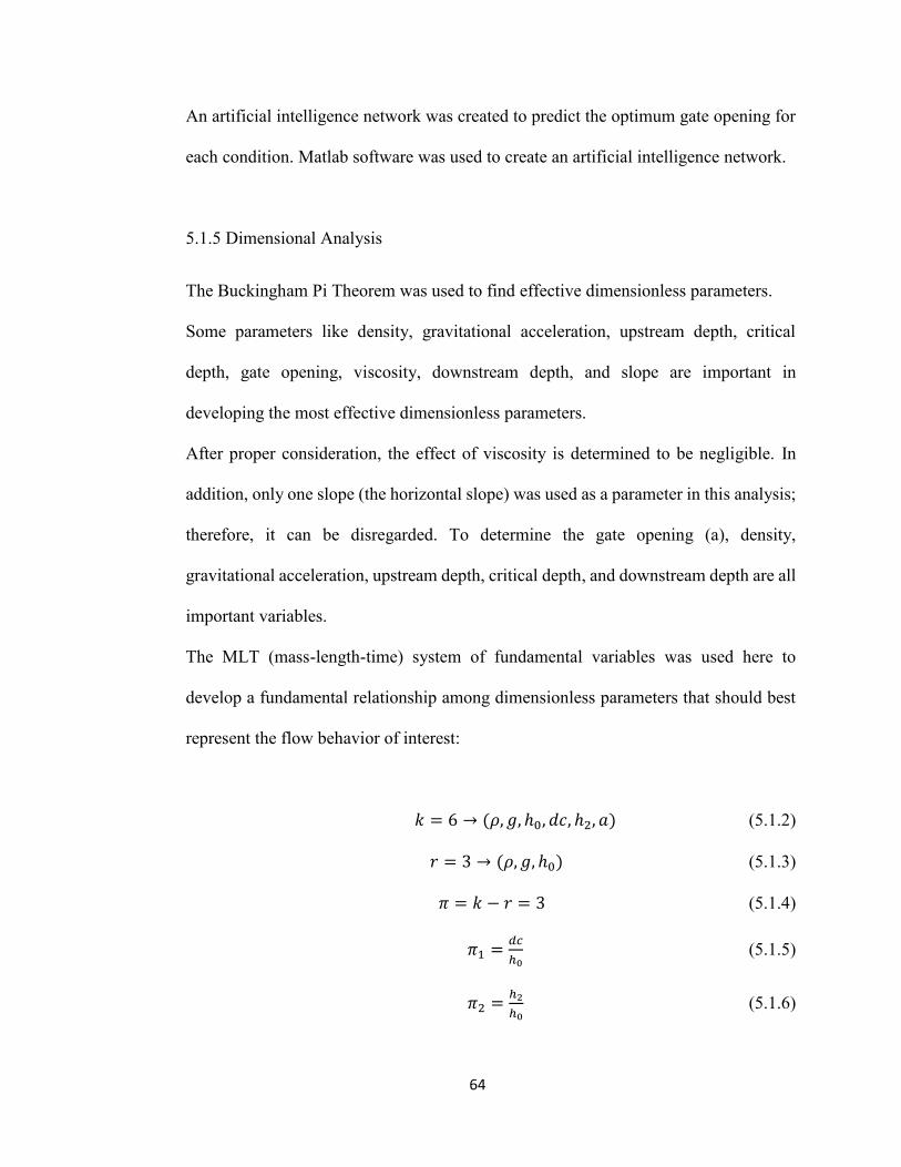
64
An artificial intelligence network was created to predict the optimum gate opening for
each condition. Matlab software was used to create an artificial intelligence network.
5.1.5 Dimensional Analysis
The Buckingham Pi Theorem was used to find effective dimensionless parameters.
Some parameters like density, gravitational acceleration, upstream depth, critical
depth, gate opening, viscosity, downstream depth, and slope are important in
developing the most effective dimensionless parameters.
After proper consideration, the effect of viscosity is determined to be negligible. In
addition, only one slope (the horizontal slope) was used as a parameter in this analysis;
therefore, it can be disregarded. To determine the gate opening (a), density,
gravitational acceleration, upstream depth, critical depth, and downstream depth are all
important variables.
The MLT (mass-length-time) system of fundamental variables was used here to
develop a fundamental relationship among dimensionless parameters that should best
represent the flow behavior of interest:
𝑘 = 6 → (𝜌, 𝑔, ℎ0, 𝑑𝑐, ℎ2, 𝑎) (5.1.2)
𝑟 = 3 → (𝜌, 𝑔, ℎ0) (5.1.3)
𝜋 = 𝑘 − 𝑟 = 3 (5.1.4)
𝜋1 =𝑑𝑐
ℎ0 (5.1.5)
𝜋2 =ℎ2
ℎ0 (5.1.6)
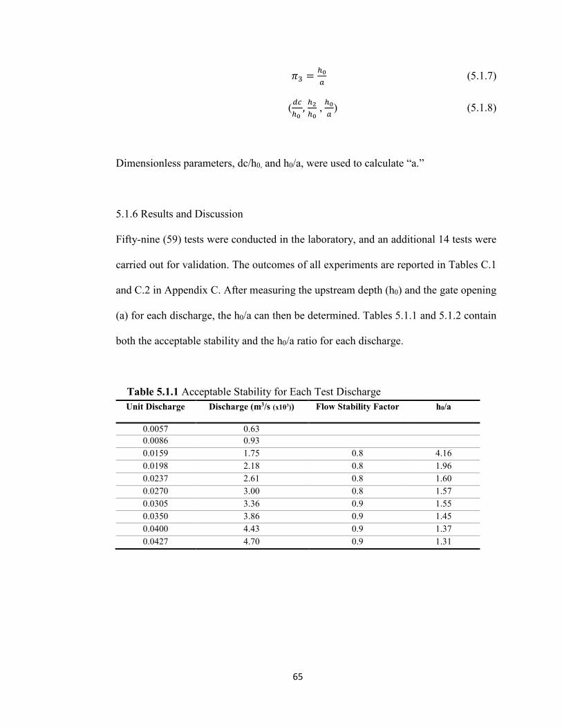
65
𝜋3 =ℎ0
𝑎 (5.1.7)
(𝑑𝑐
ℎ0 , ℎ2
ℎ0 , ℎ0
𝑎) (5.1.8)
Dimensionless parameters, dc/h0, and h0/a, were used to calculate “a.”
5.1.6 Results and Discussion
Fifty-nine (59) tests were conducted in the laboratory, and an additional 14 tests were
carried out for validation. The outcomes of all experiments are reported in Tables C.1
and C.2 in Appendix C. After measuring the upstream depth (h0) and the gate opening
(a) for each discharge, the h0/a can then be determined. Tables 5.1.1 and 5.1.2 contain
both the acceptable stability and the h0/a ratio for each discharge.
Table 5.1.1 Acceptable Stability for Each Test Discharge Unit Discharge Discharge (m3/s (x103)) Flow Stability Factor h0/a
0.0057 0.63 0.0086 0.93 0.0159 1.75 0.8 4.16 0.0198 2.18 0.8 1.96 0.0237 2.61 0.8 1.60 0.0270 3.00 0.8 1.57 0.0305 3.36 0.9 1.55 0.0350 3.86 0.9 1.45 0.0400 4.43 0.9 1.37 0.0427 4.70 0.9 1.31
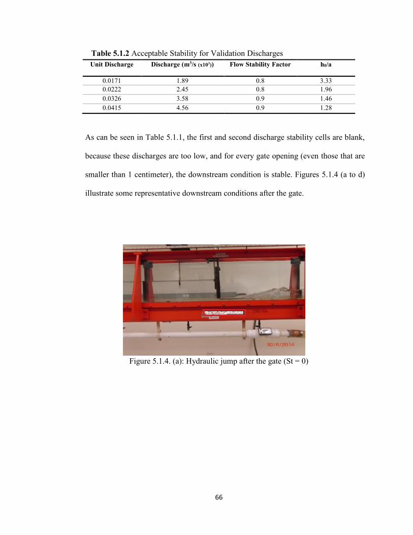
66
Table 5.1.2 Acceptable Stability for Validation Discharges Unit Discharge Discharge (m3/s (x103)) Flow Stability Factor h0/a
0.0171 1.89 0.8 3.33 0.0222 2.45 0.8 1.96 0.0326 3.58 0.9 1.46 0.0415 4.56 0.9 1.28
As can be seen in Table 5.1.1, the first and second discharge stability cells are blank,
because these discharges are too low, and for every gate opening (even those that are
smaller than 1 centimeter), the downstream condition is stable. Figures 5.1.4 (a to d)
illustrate some representative downstream conditions after the gate.
Figure 5.1.4. (a): Hydraulic jump after the gate (St = 0)
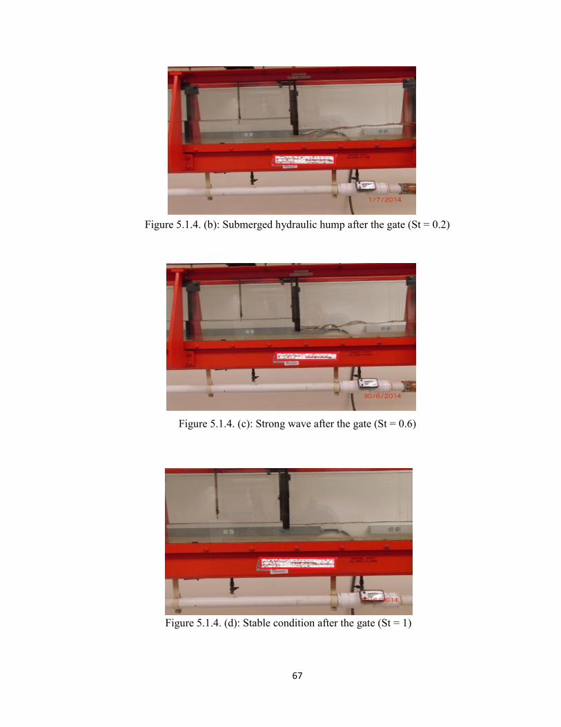
67
Figure 5.1.4. (b): Submerged hydraulic hump after the gate (St = 0.2)
Figure 5.1.4. (c): Strong wave after the gate (St = 0.6)
Figure 5.1.4. (d): Stable condition after the gate (St = 1)
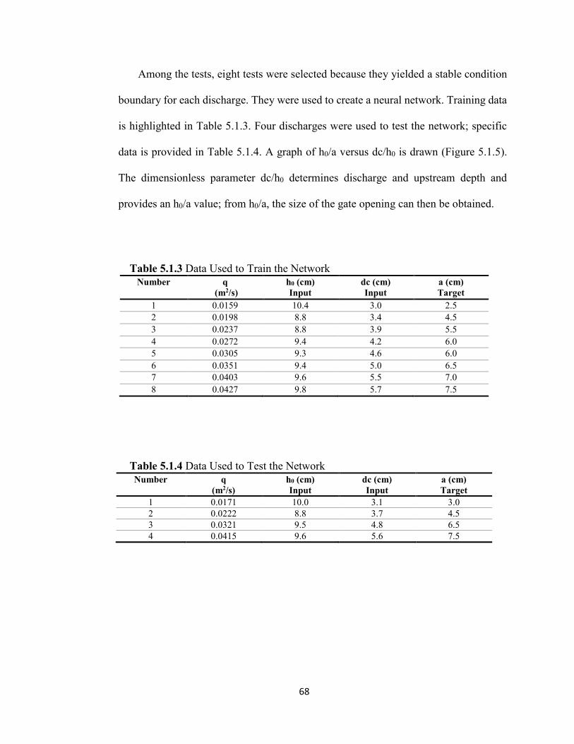
68
Among the tests, eight tests were selected because they yielded a stable condition
boundary for each discharge. They were used to create a neural network. Training data
is highlighted in Table 5.1.3. Four discharges were used to test the network; specific
data is provided in Table 5.1.4. A graph of h0/a versus dc/h0 is drawn (Figure 5.1.5).
The dimensionless parameter dc/h0 determines discharge and upstream depth and
provides an h0/a value; from h0/a, the size of the gate opening can then be obtained.
Table 5.1.3 Data Used to Train the Network Number q
(m2/s) h0 (cm) Input
dc (cm) Input
a (cm) Target
1 0.0159 10.4 3.0 2.5 2 0.0198 8.8 3.4 4.5 3 0.0237 8.8 3.9 5.5 4 0.0272 9.4 4.2 6.0 5 0.0305 9.3 4.6 6.0 6 0.0351 9.4 5.0 6.5 7 0.0403 9.6 5.5 7.0 8 0.0427 9.8 5.7 7.5
Table 5.1.4 Data Used to Test the Network Number q
(m2/s) h0 (cm) Input
dc (cm) Input
a (cm) Target
1 0.0171 10.0 3.1 3.0 2 0.0222 8.8 3.7 4.5 3 0.0321 9.5 4.8 6.5 4 0.0415 9.6 5.6 7.5
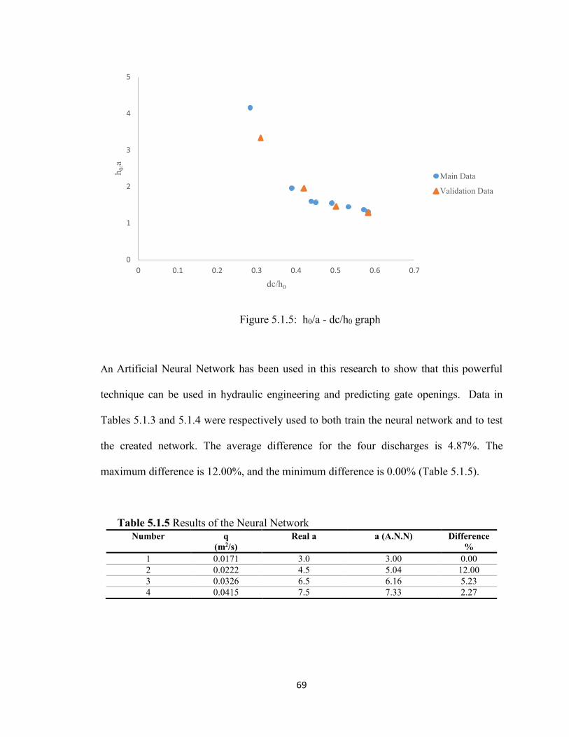
69
Figure 5.1.5: h0/a - dc/h0 graph
An Artificial Neural Network has been used in this research to show that this powerful
technique can be used in hydraulic engineering and predicting gate openings. Data in
Tables 5.1.3 and 5.1.4 were respectively used to both train the neural network and to test
the created network. The average difference for the four discharges is 4.87%. The
maximum difference is 12.00%, and the minimum difference is 0.00% (Table 5.1.5).
Table 5.1.5 Results of the Neural Network Number q
(m2/s) Real a a (A.N.N) Difference
% 1 0.0171 3.0 3.00 0.00 2 0.0222 4.5 5.04 12.00 3 0.0326 6.5 6.16 5.23 4 0.0415 7.5 7.33 2.27
0
1
2
3
4
5
0 0.1 0.2 0.3 0.4 0.5 0.6 0.7
h 0/a
dc/h0
Main Data
Validation Data
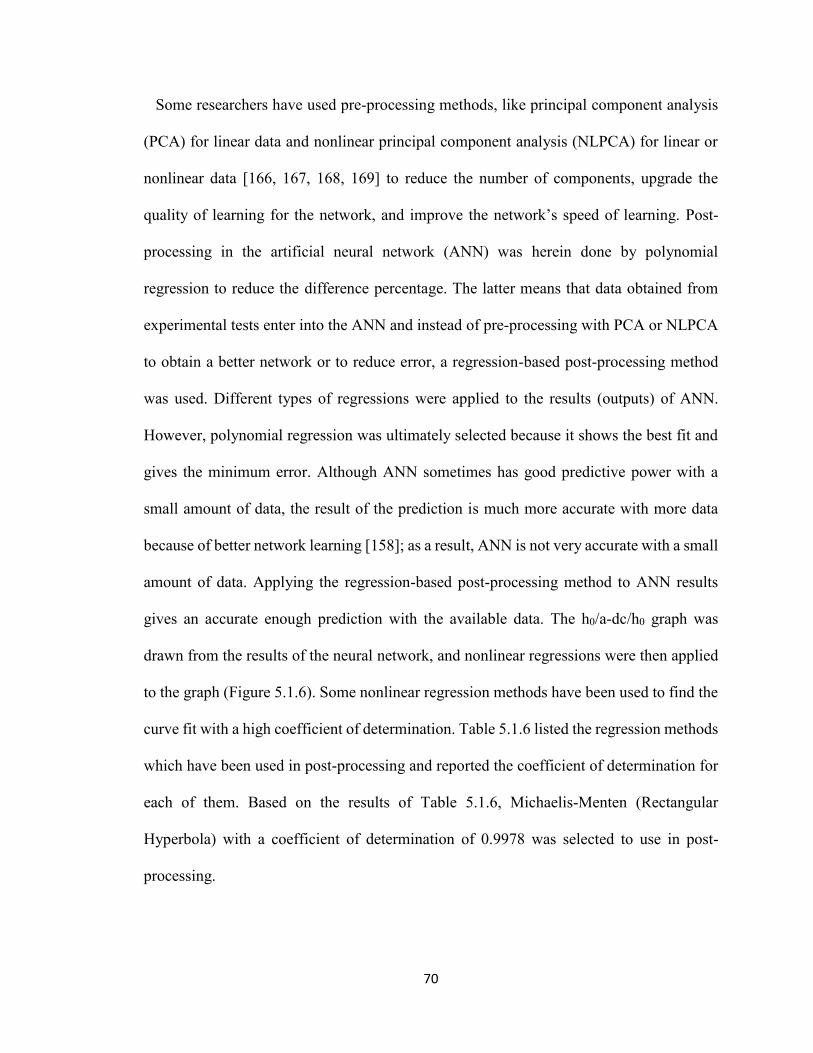
70
Some researchers have used pre-processing methods, like principal component analysis
(PCA) for linear data and nonlinear principal component analysis (NLPCA) for linear or
nonlinear data [166, 167, 168, 169] to reduce the number of components, upgrade the
quality of learning for the network, and improve the network’s speed of learning. Post-
processing in the artificial neural network (ANN) was herein done by polynomial
regression to reduce the difference percentage. The latter means that data obtained from
experimental tests enter into the ANN and instead of pre-processing with PCA or NLPCA
to obtain a better network or to reduce error, a regression-based post-processing method
was used. Different types of regressions were applied to the results (outputs) of ANN.
However, polynomial regression was ultimately selected because it shows the best fit and
gives the minimum error. Although ANN sometimes has good predictive power with a
small amount of data, the result of the prediction is much more accurate with more data
because of better network learning [158]; as a result, ANN is not very accurate with a small
amount of data. Applying the regression-based post-processing method to ANN results
gives an accurate enough prediction with the available data. The h0/a-dc/h0 graph was
drawn from the results of the neural network, and nonlinear regressions were then applied
to the graph (Figure 5.1.6). Some nonlinear regression methods have been used to find the
curve fit with a high coefficient of determination. Table 5.1.6 listed the regression methods
which have been used in post-processing and reported the coefficient of determination for
each of them. Based on the results of Table 5.1.6, Michaelis-Menten (Rectangular
Hyperbola) with a coefficient of determination of 0.9978 was selected to use in post-
processing.
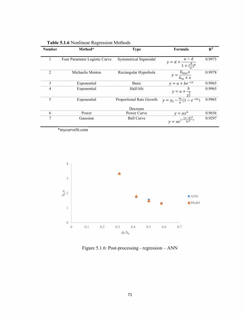
71
Table 5.1.6 Nonlinear Regression Methods Number Method* Type Formula 𝐑𝟐
1 Four Parameter Logistic Curve Symmetrical Sigmoidal 𝑦 = 𝑑 +
𝑎 − 𝑑
1 + (𝑥𝑐
)𝑏
0.9973
2 Michaelis Menten Rectangular Hyperbola 𝑦 =
𝑉𝑚𝑎𝑥𝑥
𝑘𝑚 + 𝑥 0.9978
3 Exponential Basic 𝑦 = 𝑎 + 𝑏𝑒−𝑐𝑥 0.9965 4 Exponential Half-life
𝑦 = 𝑎 +𝑏
2𝑥𝑐
0.9965
5 Exponential
Proportional Rate Growth
Decrease
𝑦 = 𝑦0 −𝑣0
𝑘(1 − 𝑒−𝑘𝑥) 0.9965
6 Power Power Curve 𝑦 = 𝑎𝑥𝑏 0.9656 7 Gaussian Bell Curve
𝑦 = 𝑎𝑒(−
(𝑥−𝑏)2
2𝑐2 ) 0.9297
*mycurvefit.com
Figure 5.1.6: Post-processing - regression – ANN
0
1
2
3
4
0 0.1 0.2 0.3 0.4 0.5 0.6 0.7
h 0/a
dc/h0
ANN
Model
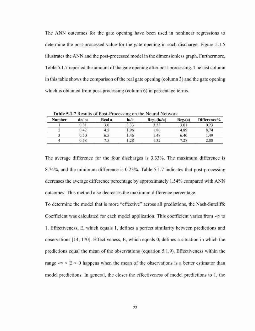
72
The ANN outcomes for the gate opening have been used in nonlinear regressions to
determine the post-processed value for the gate opening in each discharge. Figure 5.1.5
illustrates the ANN and the post-processed model in the dimensionless graph. Furthermore,
Table 5.1.7 reported the amount of the gate opening after post-processing. The last column
in this table shows the comparison of the real gate opening (column 3) and the gate opening
which is obtained from post-processing (column 6) in percentage terms.
Table 5.1.7 Results of Post-Processing on the Neural Network Number dc/ h0 Real a h0/a Reg. (h0/a) Reg.(a) Difference%
1 0.31 3.0 3.33 3.33 3.01 0.23 2 0.42 4.5 1.96 1.80 4.89 8.74 3 0.50 6.5 1.46 1.48 6.40 1.49 4 0.58 7.5 1.28 1.32 7.28 2.88
The average difference for the four discharges is 3.33%. The maximum difference is
8.74%, and the minimum difference is 0.23%. Table 5.1.7 indicates that post-processing
decreases the average difference percentage by approximately 1.54% compared with ANN
outcomes. This method also decreases the maximum difference percentage.
To determine the model that is more “effective” across all predictions, the Nash-Sutcliffe
Coefficient was calculated for each model application. This coefficient varies from - to
1. Effectiveness, E, which equals 1, defines a perfect similarity between predictions and
observations [14, 170]. Effectiveness, E, which equals 0, defines a situation in which the
predictions equal the mean of the observations (equation 5.1.9). Effectiveness within the
range - < E < 0 happens when the mean of the observations is a better estimator than
model predictions. In general, the closer the effectiveness of model predictions to 1, the
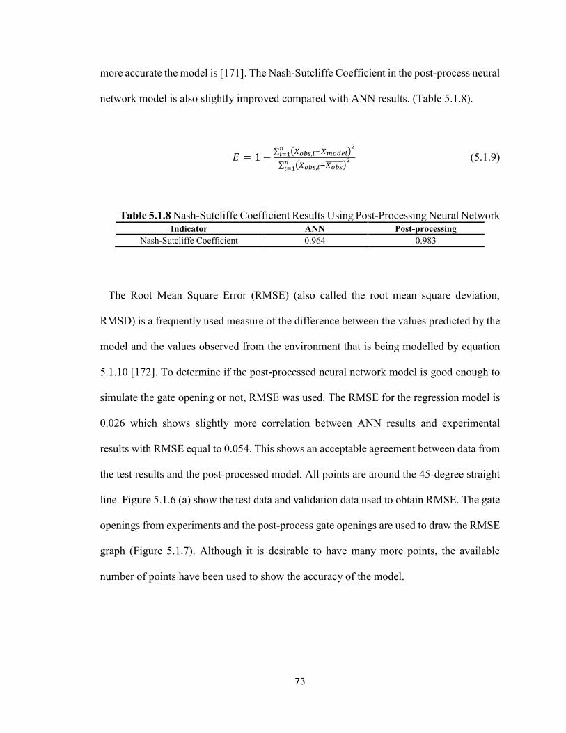
73
more accurate the model is [171]. The Nash-Sutcliffe Coefficient in the post-process neural
network model is also slightly improved compared with ANN results. (Table 5.1.8).
𝐸 = 1 −∑ (𝑋𝑜𝑏𝑠,𝑖−𝑋𝑚𝑜𝑑𝑒𝑙)
2𝑛𝑖=1
∑ (𝑋𝑜𝑏𝑠,𝑖−𝑋𝑜𝑏𝑠̅̅ ̅̅ ̅̅ ̅)2𝑛
𝑖=1
(5.1.9)
Table 5.1.8 Nash-Sutcliffe Coefficient Results Using Post-Processing Neural Network Indicator ANN Post-processing
Nash-Sutcliffe Coefficient 0.964 0.983
The Root Mean Square Error (RMSE) (also called the root mean square deviation,
RMSD) is a frequently used measure of the difference between the values predicted by the
model and the values observed from the environment that is being modelled by equation
5.1.10 [172]. To determine if the post-processed neural network model is good enough to
simulate the gate opening or not, RMSE was used. The RMSE for the regression model is
0.026 which shows slightly more correlation between ANN results and experimental
results with RMSE equal to 0.054. This shows an acceptable agreement between data from
the test results and the post-processed model. All points are around the 45-degree straight
line. Figure 5.1.6 (a) show the test data and validation data used to obtain RMSE. The gate
openings from experiments and the post-process gate openings are used to draw the RMSE
graph (Figure 5.1.7). Although it is desirable to have many more points, the available
number of points have been used to show the accuracy of the model.

74
𝑅𝑀𝑆𝐸 = √∑ (𝑋𝑜𝑏𝑠,𝑖−𝑋𝑚𝑜𝑑𝑒𝑙,𝑖)
2𝑛𝑖=1
𝑛 (5.1.10)
Figure 5.1.7: RMSE – Post-processing
0
2
4
6
8
0 2 4 6 8
Post
-Pro
cess
ing
Mod
el
Validation
75
CHAPTER 5
RESULTS & DISCUSSION
SECTION 2
FLOW STABILITY NUMBER IN VERTICAL SLUICE GATES
5.2.1 Introduction
The Flow Stability Number was defined in chapter four as a dimensionless number to
show the flow characteristics after hydraulic structures. The maximum value for this
number is one. When the value is equal to one or very close to one, the flow may be
stable. There are three conditions for the flow to be stable. These three conditions were
presented in chapter four. When the flow is stable, it means that the channel is safe
from surface flow fluctuations and also erosion. The experiments were conducted in
two laboratories; the Fluid Mechanics Laboratory at Florida International University
and the Center for Research in Water Resources at the University of Texas at Austin.
Two laboratories were selected for this research to see the scale effect. Moreover,
sediment transport was considered in the second laboratory to find an acceptable range
for the Flow Stability Number.
5.2.2 Experiments (Set One)
A total of 10 experiments (10 discharges) were selected from the gate results to find
the Flow Stability Number. These experiments were performed in a narrow flume,
located at the Fluid Mechanics Laboratory of the Civil and Environmental Engineering
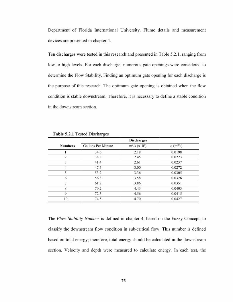
76
Department of Florida International University. Flume details and measurement
devices are presented in chapter 4.
Ten discharges were tested in this research and presented in Table 5.2.1, ranging from
low to high levels. For each discharge, numerous gate openings were considered to
determine the Flow Stability. Finding an optimum gate opening for each discharge is
the purpose of this research. The optimum gate opening is obtained when the flow
condition is stable downstream. Therefore, it is necessary to define a stable condition
in the downstream section.
Table 5.2.1 Tested Discharges Discharges Numbers Gallons Per Minute
(GPM)
m3/s (x103) q (m2/s)
1 34.6 2.18 0.0198 2 38.8 2.45 0.0223 3 41.4 2.61 0.0237 4 47.5 3.00 0.0272 5 53.2 3.36 0.0305 6 56.8 3.58 0.0326 7 61.2 3.86 0.0351 8 70.2 4.43 0.0403 9 72.3 4.56 0.0415 10 74.5 4.70 0.0427
The Flow Stability Number is defined in chapter 4, based on the Fuzzy Concept, to
classify the downstream flow condition in sub-critical flow. This number is defined
based on total energy; therefore, total energy should be calculated in the downstream
section. Velocity and depth were measured to calculate energy. In each test, the
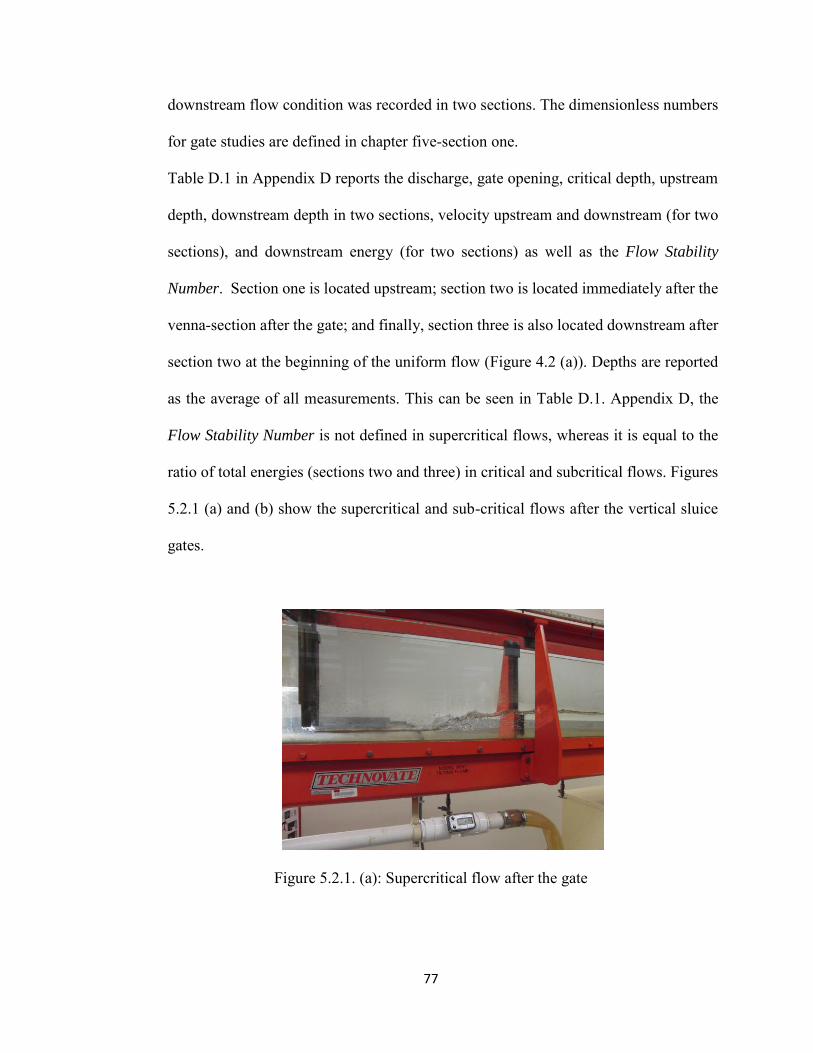
77
downstream flow condition was recorded in two sections. The dimensionless numbers
for gate studies are defined in chapter five-section one.
Table D.1 in Appendix D reports the discharge, gate opening, critical depth, upstream
depth, downstream depth in two sections, velocity upstream and downstream (for two
sections), and downstream energy (for two sections) as well as the Flow Stability
Number. Section one is located upstream; section two is located immediately after the
venna-section after the gate; and finally, section three is also located downstream after
section two at the beginning of the uniform flow (Figure 4.2 (a)). Depths are reported
as the average of all measurements. This can be seen in Table D.1. Appendix D, the
Flow Stability Number is not defined in supercritical flows, whereas it is equal to the
ratio of total energies (sections two and three) in critical and subcritical flows. Figures
5.2.1 (a) and (b) show the supercritical and sub-critical flows after the vertical sluice
gates.
Figure 5.2.1. (a): Supercritical flow after the gate
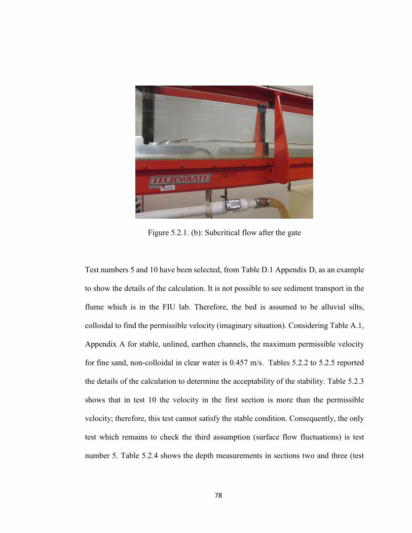
78
Figure 5.2.1. (b): Subcritical flow after the gate
Test numbers 5 and 10 have been selected, from Table D.1 Appendix D, as an example
to show the details of the calculation. It is not possible to see sediment transport in the
flume which is in the FIU lab. Therefore, the bed is assumed to be alluvial silts,
colloidal to find the permissible velocity (imaginary situation). Considering Table A.1,
Appendix A for stable, unlined, earthen channels, the maximum permissible velocity
for fine sand, non-colloidal in clear water is 0.457 m/s. Tables 5.2.2 to 5.2.5 reported
the details of the calculation to determine the acceptability of the stability. Table 5.2.3
shows that in test 10 the velocity in the first section is more than the permissible
velocity; therefore, this test cannot satisfy the stable condition. Consequently, the only
test which remains to check the third assumption (surface flow fluctuations) is test
number 5. Table 5.2.4 shows the depth measurements in sections two and three (test
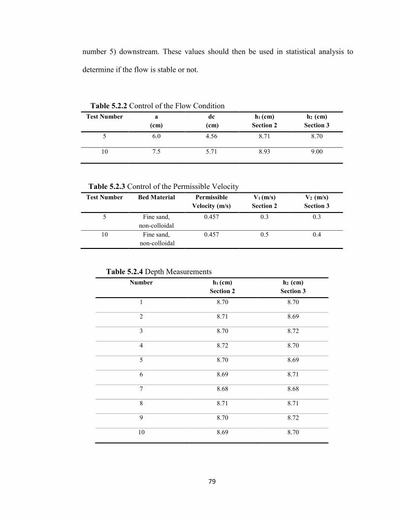
79
number 5) downstream. These values should then be used in statistical analysis to
determine if the flow is stable or not.
Table 5.2.2 Control of the Flow Condition Test Number a
(cm) dc
(cm) h1 (cm)
Section 2 h2 (cm)
Section 3
5 6.0 4.56 8.71 8.70
10 7.5 5.71 8.93 9.00
Table 5.2.3 Control of the Permissible Velocity Test Number Bed Material Permissible
Velocity (m/s) V1 (m/s)
Section 2 V2 (m/s)
Section 3
5 Fine sand, non-colloidal
0.457 0.3 0.3
10 Fine sand, non-colloidal
0.457 0.5 0.4
Table 5.2.4 Depth Measurements Number h1 (cm)
Section 2 h2 (cm)
Section 3
1 8.70 8.70
2 8.71 8.69
3 8.70 8.72
4 8.72 8.70
5 8.70 8.69
6 8.69 8.71
7 8.68 8.68
8 8.71 8.71
9 8.70 8.72
10 8.69 8.70

80
Table 5.2.5 Two-sided t-test t-test Value H0
Ha P-Value Result Explanation
Section 2 versus
section 3 *The average of section 2 is equal to the average of section 3
H0
is false 0.7223 Do not
reject 𝐻0
There is no evidence to conclude that the average of section 2 is different from the average of section 3. So, it is reasonable to assume that the two averages are equal. ●Assume 𝛼 = 0.005
●Degree of
freedom: n-2=18
●t value :
-0.36116
●95% confidence interval -0.013648584 0.009648584
*the mean of section 2 is 8.700 and the mean of section 3 is 8.702
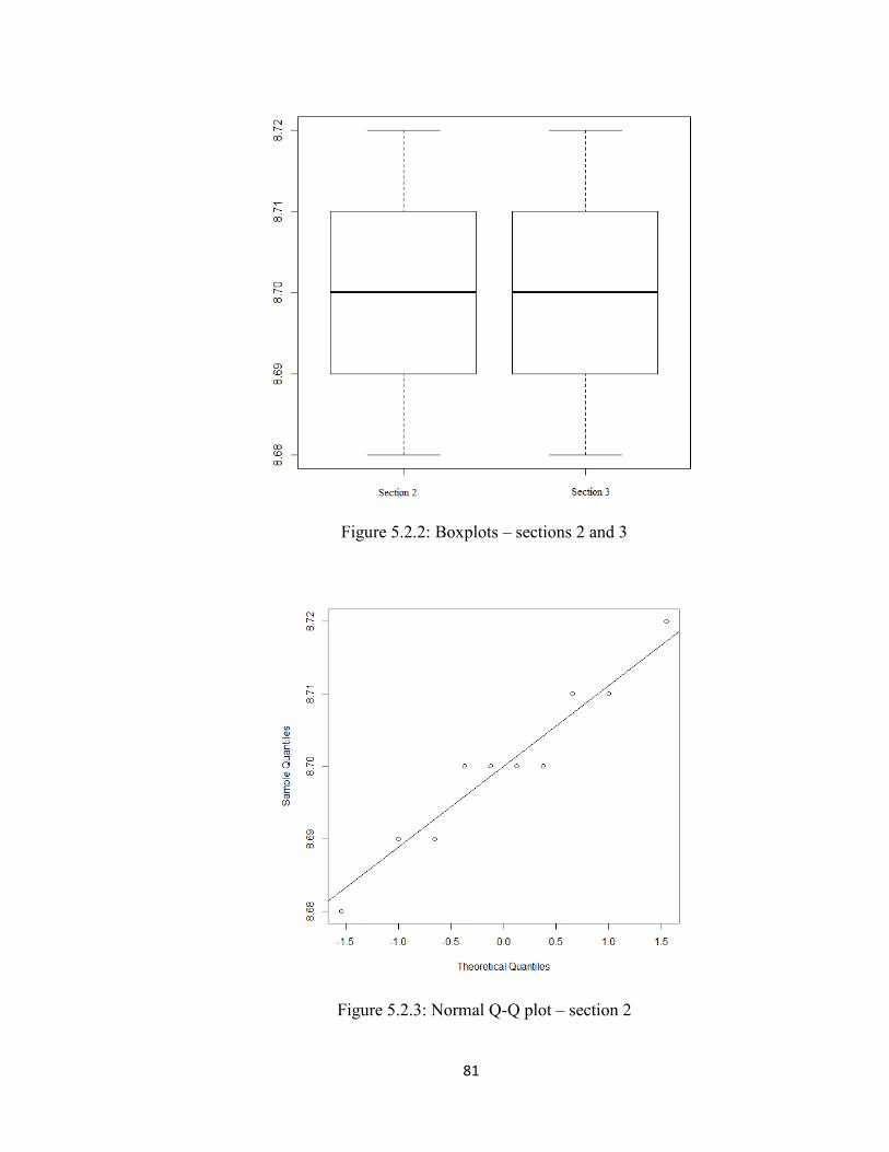
81
Figure 5.2.2: Boxplots – sections 2 and 3
Figure 5.2.3: Normal Q-Q plot – section 2
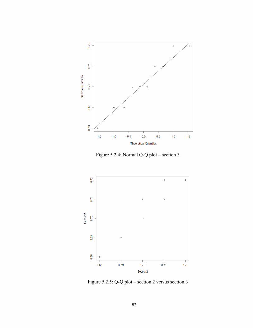
82
Figure 5.2.4: Normal Q-Q plot – section 3
Figure 5.2.5: Q-Q plot – section 2 versus section 3
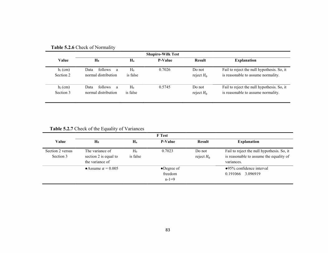
83
Table 5.2.6 Check of Normality Shapiro-Wilk Test Value H0
Ha P-Value Result Explanation
h1 (cm)
Section 2 Data follows a normal distribution
H0
is false 0.7026 Do not
reject 𝐻0
Fail to reject the null hypothesis. So, it is reasonable to assume normality.
h2 (cm)
Section 3 Data follows a normal distribution
H0
is false
0.5745 Do not reject 𝐻0
Fail to reject the null hypothesis. So, it is reasonable to assume normality.
Table 5.2.7 Check of the Equality of Variances F Test Value H0
Ha P-Value Result Explanation
Section 2 versus
Section 3 The variance of section 2 is equal to the variance of section 3
H0
is false 0.7023 Do not
reject 𝐻0
Fail to reject the null hypothesis. So, it is reasonable to assume the equality of variances.
●Assume 𝛼 = 0.005
●Degree of freedom n-1=9
●95% confidence interval 0.191066 3.096919
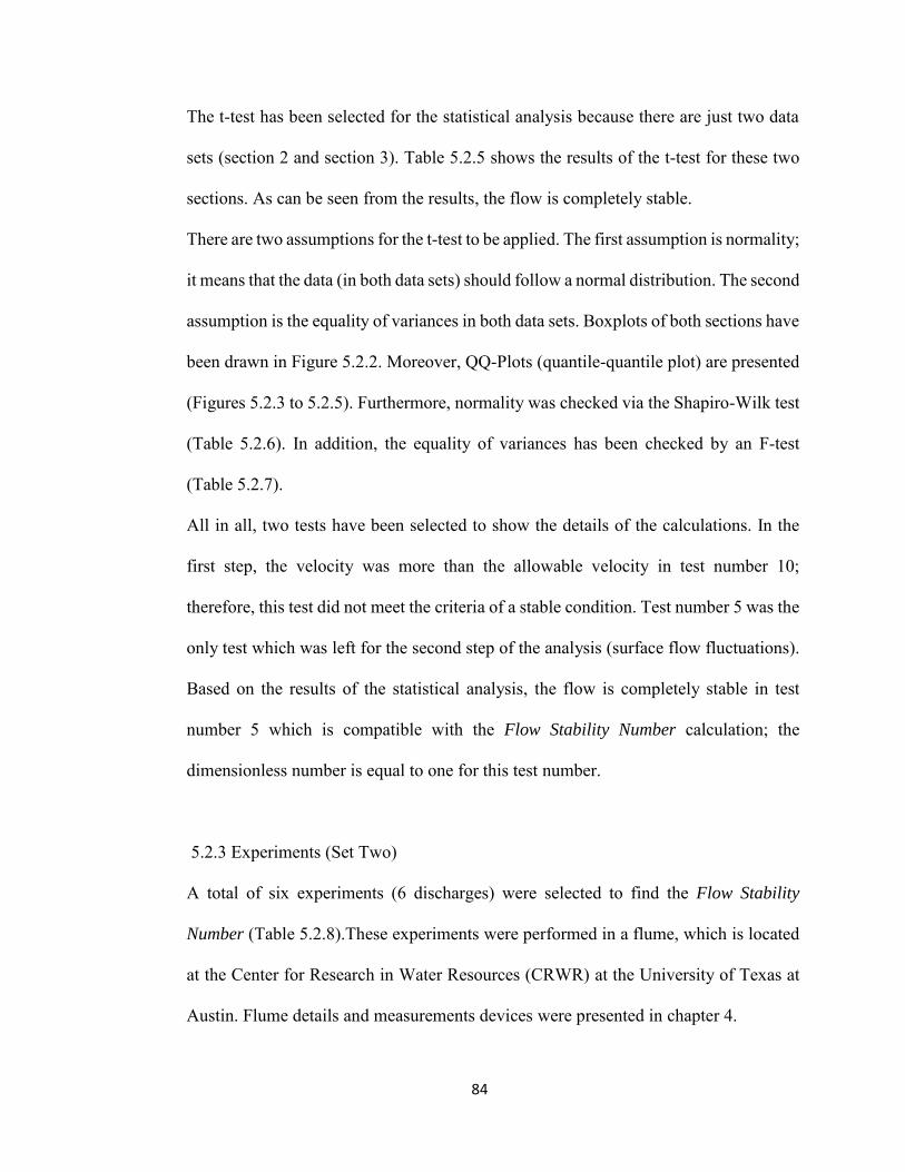
84
The t-test has been selected for the statistical analysis because there are just two data
sets (section 2 and section 3). Table 5.2.5 shows the results of the t-test for these two
sections. As can be seen from the results, the flow is completely stable.
There are two assumptions for the t-test to be applied. The first assumption is normality;
it means that the data (in both data sets) should follow a normal distribution. The second
assumption is the equality of variances in both data sets. Boxplots of both sections have
been drawn in Figure 5.2.2. Moreover, QQ-Plots (quantile-quantile plot) are presented
(Figures 5.2.3 to 5.2.5). Furthermore, normality was checked via the Shapiro-Wilk test
(Table 5.2.6). In addition, the equality of variances has been checked by an F-test
(Table 5.2.7).
All in all, two tests have been selected to show the details of the calculations. In the
first step, the velocity was more than the allowable velocity in test number 10;
therefore, this test did not meet the criteria of a stable condition. Test number 5 was the
only test which was left for the second step of the analysis (surface flow fluctuations).
Based on the results of the statistical analysis, the flow is completely stable in test
number 5 which is compatible with the Flow Stability Number calculation; the
dimensionless number is equal to one for this test number.
5.2.3 Experiments (Set Two)
A total of six experiments (6 discharges) were selected to find the Flow Stability
Number (Table 5.2.8).These experiments were performed in a flume, which is located
at the Center for Research in Water Resources (CRWR) at the University of Texas at
Austin. Flume details and measurements devices were presented in chapter 4.
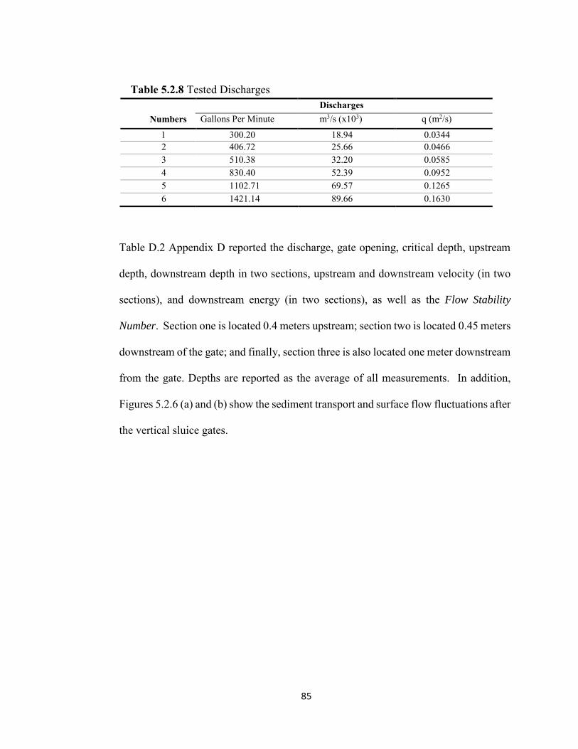
85
Table 5.2.8 Tested Discharges
Discharges Numbers Gallons Per Minute m3/s (x103) q (m2/s)
1 300.20 18.94 0.0344 2 406.72 25.66 0.0466 3 510.38 32.20 0.0585 4 830.40 52.39 0.0952 5 1102.71 69.57 0.1265 6 1421.14 89.66 0.1630
Table D.2 Appendix D reported the discharge, gate opening, critical depth, upstream
depth, downstream depth in two sections, upstream and downstream velocity (in two
sections), and downstream energy (in two sections), as well as the Flow Stability
Number. Section one is located 0.4 meters upstream; section two is located 0.45 meters
downstream of the gate; and finally, section three is also located one meter downstream
from the gate. Depths are reported as the average of all measurements. In addition,
Figures 5.2.6 (a) and (b) show the sediment transport and surface flow fluctuations after
the vertical sluice gates.
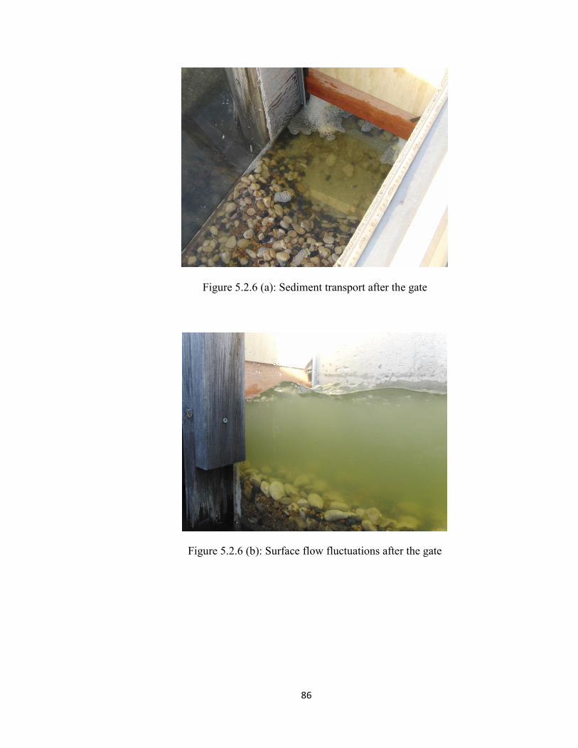
86
Figure 5.2.6 (a): Sediment transport after the gate
Figure 5.2.6 (b): Surface flow fluctuations after the gate

87
Test number 6 was selected as an example to show the details of the calculation. The
bed is a mixture of limestone pebbles, basalt pebbles, and brown pea gravel.
Considering Table A.1. Appendix A, for stable, unlined, earthen channels, the
maximum permissible velocity for coarse gravel, non-colloidal, and fine gravel in clear
water are 1.220 and 0.762 m/s, respectively. The minimum value is taken in this study
as a safety factor. Tables 5.2.9 to 5.2.12 reported the details of the calculation to
determine the acceptability of the stability. As can be seen from Table 5.2.9, the depths
in both the second and the third section are more than the critical depth; therefore, the
first assumption is satisfied. Table 5.2.10 shows that the velocities in both sections are
less than the permissible velocity; consequently, the test is eligible for checking the
third assumption (surface flow fluctuations). Table 5.2.11 shows the depth
measurements in sections two and three (test number 6) downstream. These values
should then be used in the statistical analysis to determine if the flow is stable or not.
Table 5.2.9 Control of the Flow Condition Test Number a
(cm) dc
(cm) h1 (cm)
Section 2 h2 (cm)
Section 3
6 23.0 13.94 21.91 21.91
Table 5.2.10 Control of the Permissible Velocity Test Number Bed Material Permissible
Velocity (m/s) V1 (m/s)
Section 2 V2 (m/s)
Section 3
6 Fine gravel 0.762 0.74 0.74
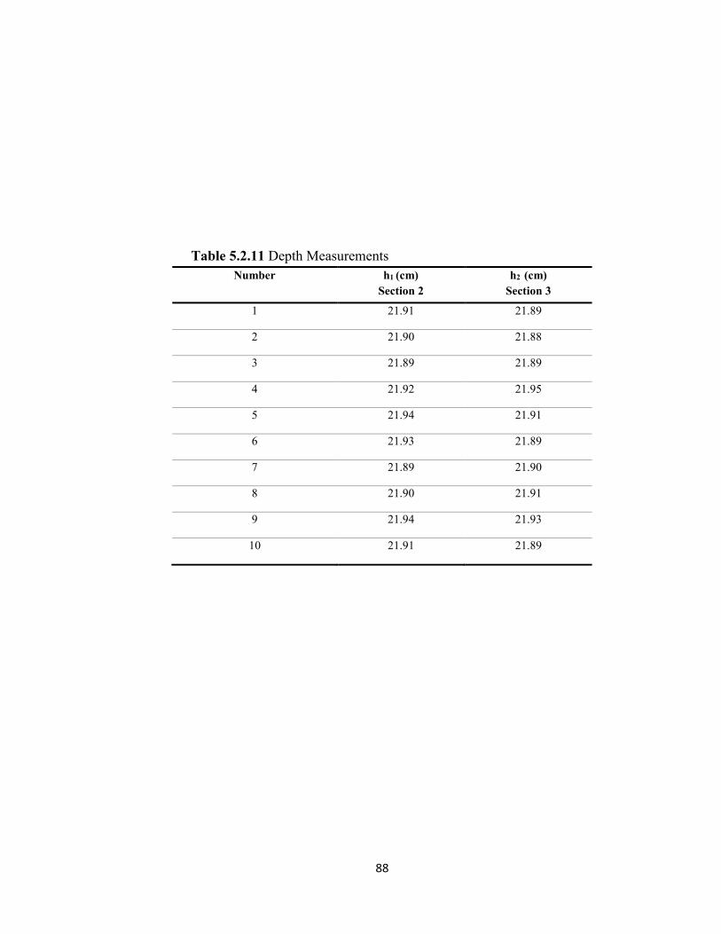
88
Table 5.2.11 Depth Measurements Number h1 (cm)
Section 2 h2 (cm)
Section 3
1 21.91 21.89
2 21.90 21.88
3 21.89 21.89
4 21.92 21.95
5 21.94 21.91
6 21.93 21.89
7 21.89 21.90
8 21.90 21.91
9 21.94 21.93
10 21.91 21.89
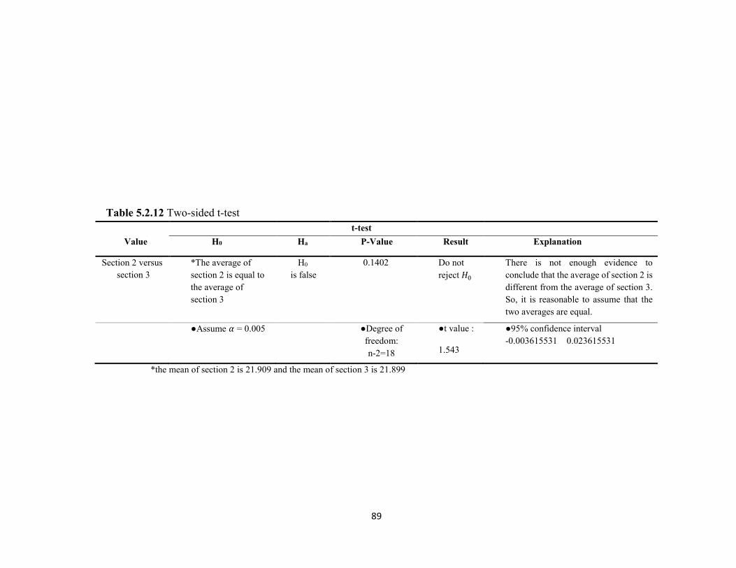
89
Table 5.2.12 Two-sided t-test t-test Value H0
Ha P-Value Result Explanation
Section 2 versus
section 3 *The average of section 2 is equal to the average of section 3
H0
is false 0.1402 Do not
reject 𝐻0
There is not enough evidence to conclude that the average of section 2 is different from the average of section 3. So, it is reasonable to assume that the two averages are equal.
●Assume 𝛼 = 0.005
●Degree of freedom: n-2=18
●t value :
1.543
●95% confidence interval -0.003615531 0.023615531
*the mean of section 2 is 21.909 and the mean of section 3 is 21.899
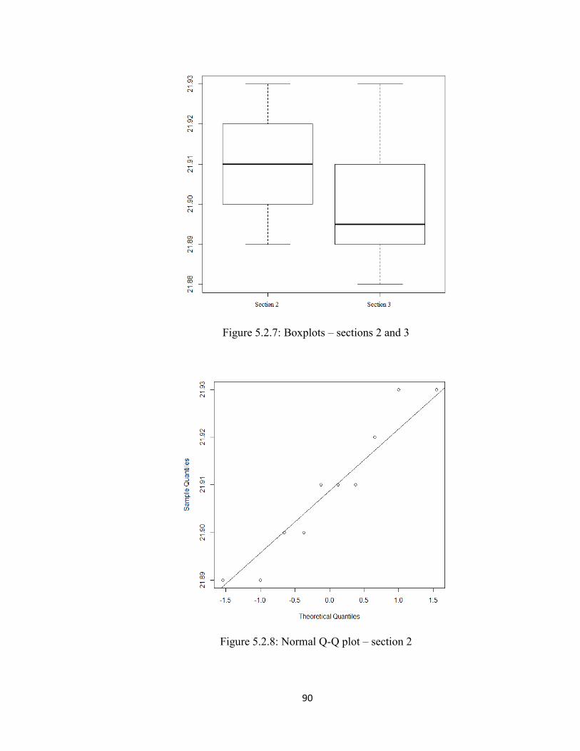
90
Figure 5.2.7: Boxplots – sections 2 and 3
Figure 5.2.8: Normal Q-Q plot – section 2
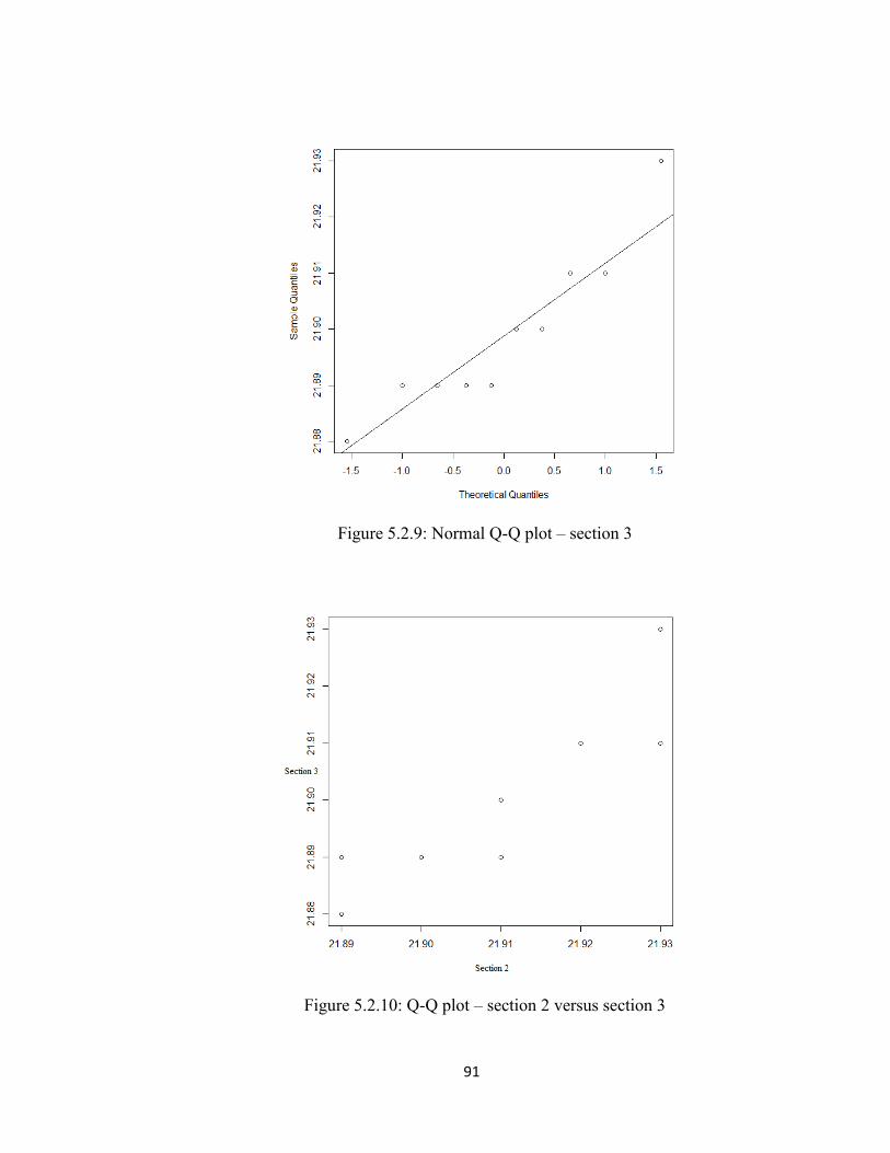
91
Figure 5.2.9: Normal Q-Q plot – section 3
Figure 5.2.10: Q-Q plot – section 2 versus section 3

92
Table 5.2.13 Check of Normality Shapiro-Wilk Test Value H0
Ha P-Value Result Explanation
h1 (cm)
Section 2 Data follows a normal distribution
H0
is false 0.3296 Do not
reject 𝐻0
Fail to reject the null hypothesis. So, it is reasonable to assume normality.
h2 (cm)
Section 3 Data follows a normal distribution
H0
is false
0.2045 Do not reject 𝐻0
Fail to reject the null hypothesis. So, it is reasonable to assume normality.
Table 5.2.14 Check of the Equality of Variances F Test Value H0
Ha P-Value Result Explanation
Section 2 versus
section 3 The variance of section 2 is equal to the variance of section 3
H0
is false 1 Do not
reject 𝐻0
Fail to reject the null hypothesis. So, it is reasonable to assume the equality of variances.
●Assume 𝛼 = 0.005
●Degree of freedom n-1=9
●95% confidence interval 0.2483859 4.0259942
93
The t-test has been selected for the statistical analysis because there are just two data
sets (section 2 and section 3). Table 5.2.12 shows the results of the t-test for these two
sections. As can be seen from the results, the flow is completely stable.
There are two assumptions for the t-test to be applied. The first assumption is normality;
it means that the data (in both data sets) should follow a normal distribution. The second
assumption is the equality of variances in both data sets. Boxplots of both sections have
been drawn as Figure 5.2.7. Moreover, QQ-Plots (quantile-quantile plot) are presented
in both sections (Figures 5.2.8 to 5.2.10). Furthermore, normality was checked by the
Shapiro-Wilk test (Table 5.2.13). In addition, the equality of variances was checked by
an F-test (Table 5.2.14).
Based on the results of the statistical analysis, the flow is completely stable in test
number 6 which is compatible with the Flow Stability Number calculation; the
dimensionless number is equal to one for this test number.
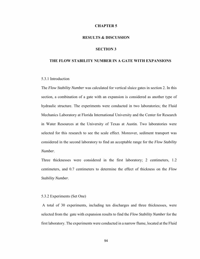
94
CHAPTER 5
RESULTS & DISCUSSION
SECTION 3
THE FLOW STABILITY NUMBER IN A GATE WITH EXPANSIONS
5.3.1 Introduction
The Flow Stability Number was calculated for vertical sluice gates in section 2. In this
section, a combination of a gate with an expansion is considered as another type of
hydraulic structure. The experiments were conducted in two laboratories; the Fluid
Mechanics Laboratory at Florida International University and the Center for Research
in Water Resources at the University of Texas at Austin. Two laboratories were
selected for this research to see the scale effect. Moreover, sediment transport was
considered in the second laboratory to find an acceptable range for the Flow Stability
Number.
Three thicknesses were considered in the first laboratory; 2 centimeters, 1.2
centimeters, and 0.7 centimeters to determine the effect of thickness on the Flow
Stability Number.
5.3.2 Experiments (Set One)
A total of 30 experiments, including ten discharges and three thicknesses, were
selected from the gate with expansion results to find the Flow Stability Number for the
first laboratory. The experiments were conducted in a narrow flume, located at the Fluid
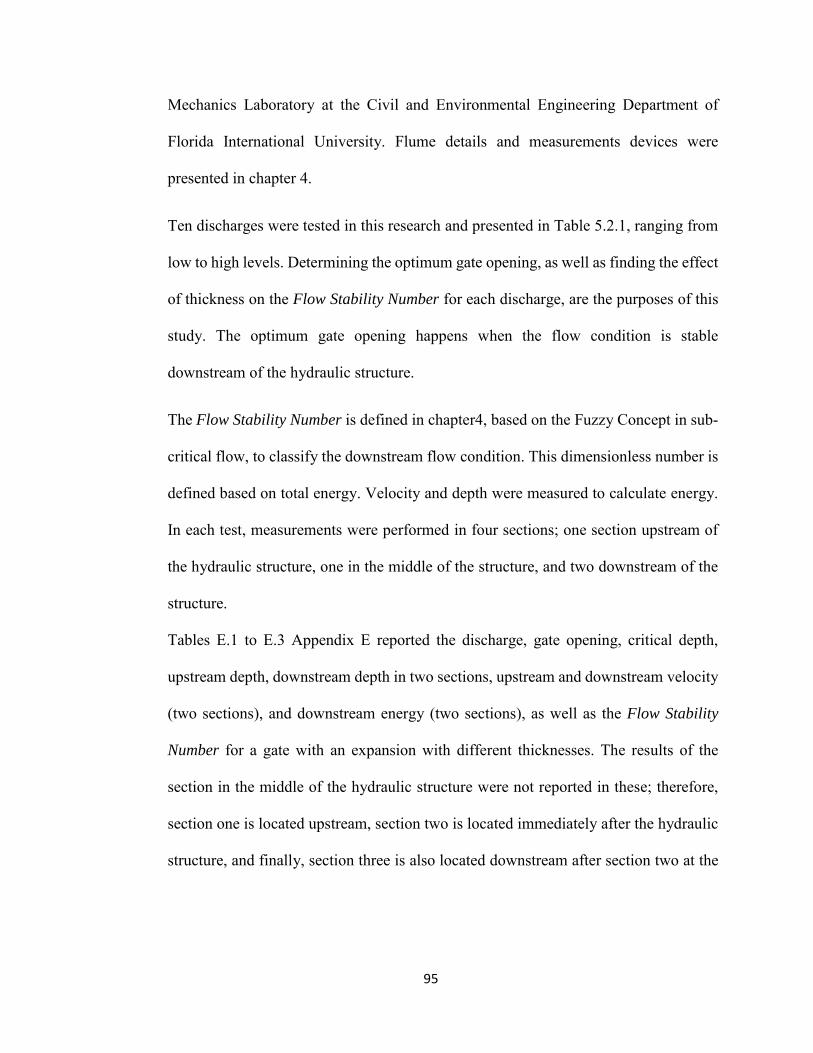
95
Mechanics Laboratory at the Civil and Environmental Engineering Department of
Florida International University. Flume details and measurements devices were
presented in chapter 4.
Ten discharges were tested in this research and presented in Table 5.2.1, ranging from
low to high levels. Determining the optimum gate opening, as well as finding the effect
of thickness on the Flow Stability Number for each discharge, are the purposes of this
study. The optimum gate opening happens when the flow condition is stable
downstream of the hydraulic structure.
The Flow Stability Number is defined in chapter4, based on the Fuzzy Concept in sub-
critical flow, to classify the downstream flow condition. This dimensionless number is
defined based on total energy. Velocity and depth were measured to calculate energy.
In each test, measurements were performed in four sections; one section upstream of
the hydraulic structure, one in the middle of the structure, and two downstream of the
structure.
Tables E.1 to E.3 Appendix E reported the discharge, gate opening, critical depth,
upstream depth, downstream depth in two sections, upstream and downstream velocity
(two sections), and downstream energy (two sections), as well as the Flow Stability
Number for a gate with an expansion with different thicknesses. The results of the
section in the middle of the hydraulic structure were not reported in these; therefore,
section one is located upstream, section two is located immediately after the hydraulic
structure, and finally, section three is also located downstream after section two at the
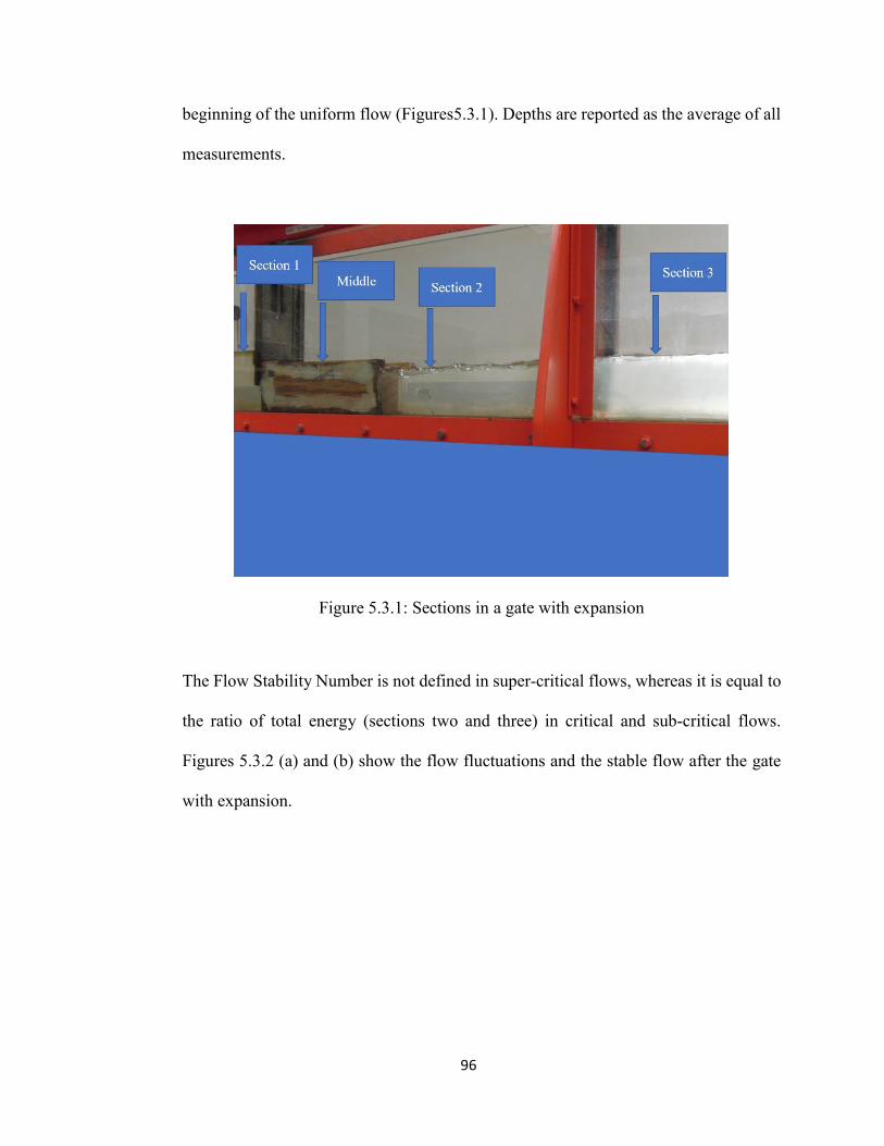
96
beginning of the uniform flow (Figures5.3.1). Depths are reported as the average of all
measurements.
Figure 5.3.1: Sections in a gate with expansion
The Flow Stability Number is not defined in super-critical flows, whereas it is equal to
the ratio of total energy (sections two and three) in critical and sub-critical flows.
Figures 5.3.2 (a) and (b) show the flow fluctuations and the stable flow after the gate
with expansion.
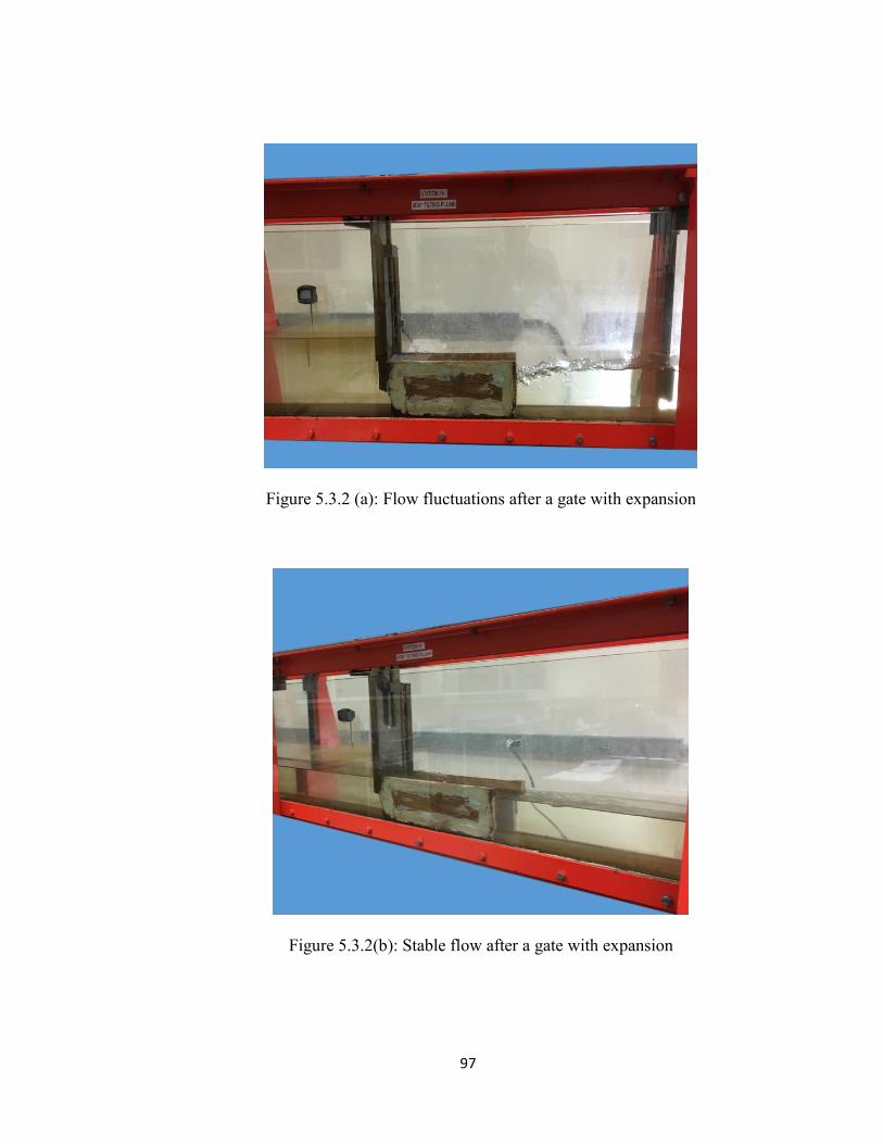
97
Figure 5.3.2 (a): Flow fluctuations after a gate with expansion
Figure 5.3.2(b): Stable flow after a gate with expansion

98
Test numbers 2, 7, 8, and 10 from Table E.1 Appendix E have been selected as an
example to show the details of the calculation. It is not possible to see the sediment
transport in the flume which is at the FIU lab. Therefore, the bed is assumed to be
alluvial silts, colloidal to find the permissible velocity (hypothetical situation).
Considering Table A.1, Appendix A for stable, unlined, earthen channels, the
maximum permissible velocity for fine sand, non-colloidal in clear water is 0.457 m/s.
Tables 5.3.4 to 5.3.7 reported the details of the calculation to determine the
acceptability of the stability. As can be seen from Table 5.3.1, the depths in the second
section of tests 8 and 10 are less than the critical depth; hence, the flow is super-critical
and cannot be stable. According to the results of Table 5.2.1, test numbers 8 and 10
will be excluded from the rest of the calculations. Table 5.2.2 shows that in test 7 the
velocity in the second section is more than the permissible velocity; therefore, this test
cannot satisfy the stability condition. Consequently, the only test which remains to
check the third assumption (surface flow fluctuations) is test number 2. Table 5.3.3
shows the depth measurements in sections two and three (test number 2) downstream.
These values should then be used in statistical analysis to determine if the flow is stable
or not.
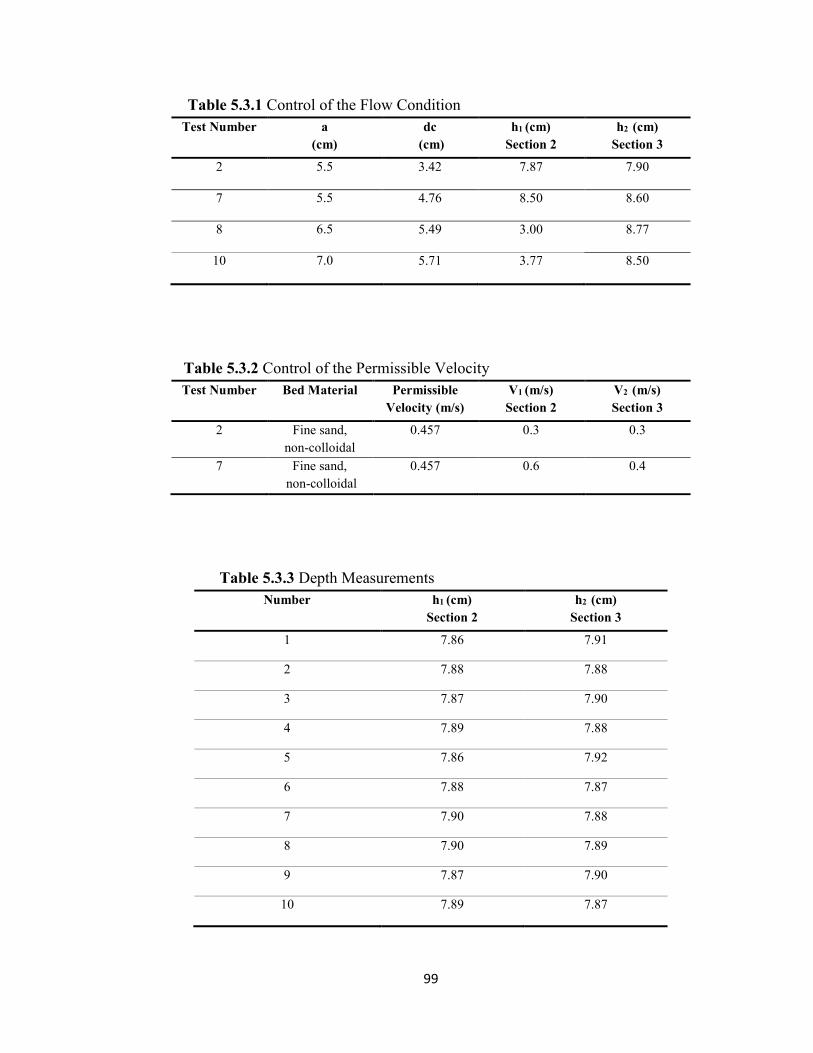
99
Table 5.3.1 Control of the Flow Condition Test Number a
(cm) dc
(cm) h1 (cm)
Section 2 h2 (cm)
Section 3
2 5.5 3.42 7.87 7.90
7 5.5 4.76 8.50 8.60
8 6.5 5.49 3.00 8.77
10 7.0 5.71 3.77 8.50
Table 5.3.2 Control of the Permissible Velocity Test Number Bed Material Permissible
Velocity (m/s) V1 (m/s)
Section 2 V2 (m/s)
Section 3
2 Fine sand, non-colloidal
0.457 0.3 0.3
7 Fine sand, non-colloidal
0.457 0.6 0.4
Table 5.3.3 Depth Measurements Number h1 (cm)
Section 2 h2 (cm)
Section 3
1 7.86 7.91
2 7.88 7.88
3 7.87 7.90
4 7.89 7.88
5 7.86 7.92
6 7.88 7.87
7 7.90 7.88
8 7.90 7.89
9 7.87 7.90
10 7.89 7.87
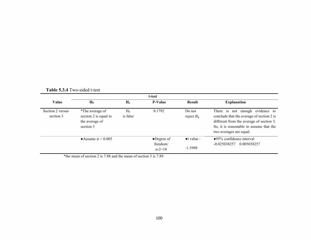
100
Table 5.3.4 Two-sided t-test t-test Value H0
Ha P-Value Result Explanation
Section 2 versus
section 3 *The average of section 2 is equal to the average of section 3
H0
is false 0.1792 Do not
reject 𝐻0
There is not enough evidence to conclude that the average of section 2 is different from the average of section 3. So, it is reasonable to assume that the two averages are equal. ●Assume 𝛼 = 0.005
●Degree of
freedom: n-2=18
●t value :
-1.3988
●95% confidence interval -0.025038257 0.005038257
*the mean of section 2 is 7.88 and the mean of section 3 is 7.89
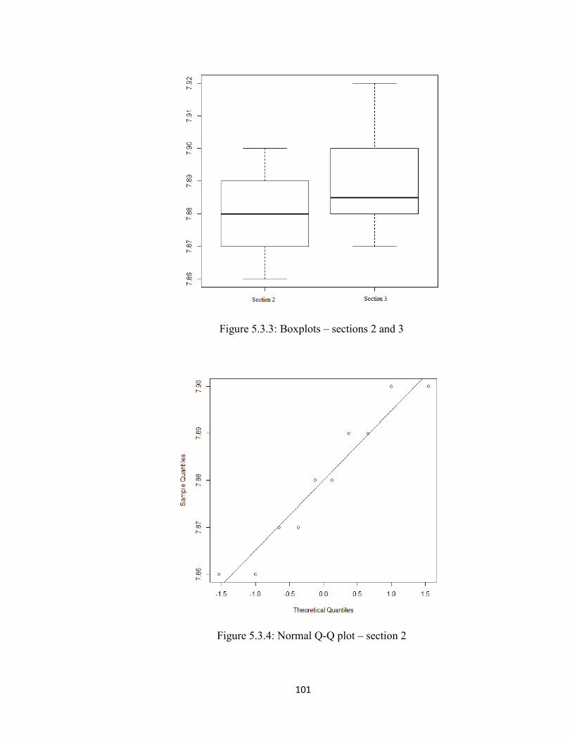
101
Figure 5.3.3: Boxplots – sections 2 and 3
Figure 5.3.4: Normal Q-Q plot – section 2
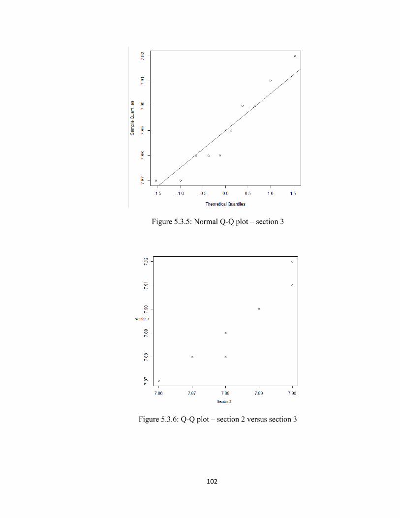
102
Figure 5.3.5: Normal Q-Q plot – section 3
Figure 5.3.6: Q-Q plot – section 2 versus section 3

103
Table 5.3.5 Check of Normality Shapiro-Wilk Test Value H0
Ha P-Value Result Explanation
h1 (cm)
Section 2 Data follows a normal distribution
H0
is false 0.3411 Do not
reject 𝐻0
Fail to reject the null hypothesis. So, it is reasonable to assume normality.
h2 (cm)
Section 3 Data follows a normal distribution
H0
is false
0.3828 Do not reject 𝐻0
Fail to reject the null hypothesis. So, it is reasonable to assume normality.
Table 5.3.6 Check of the Equality of Variances F Test Value H0
Ha P-Value Result Explanation
Section 2 versus
section 3 The variance of section 2 is equal to the variance of section 3
H0
is false 0.7023 Do not
reject 𝐻0
Fail to reject the null hypothesis. So, it is reasonable to assume the equality of variances.
●Assume 𝛼 = 0.005
●Degree of freedom n-1=9
●95% confidence interval 0.191066 3.096919
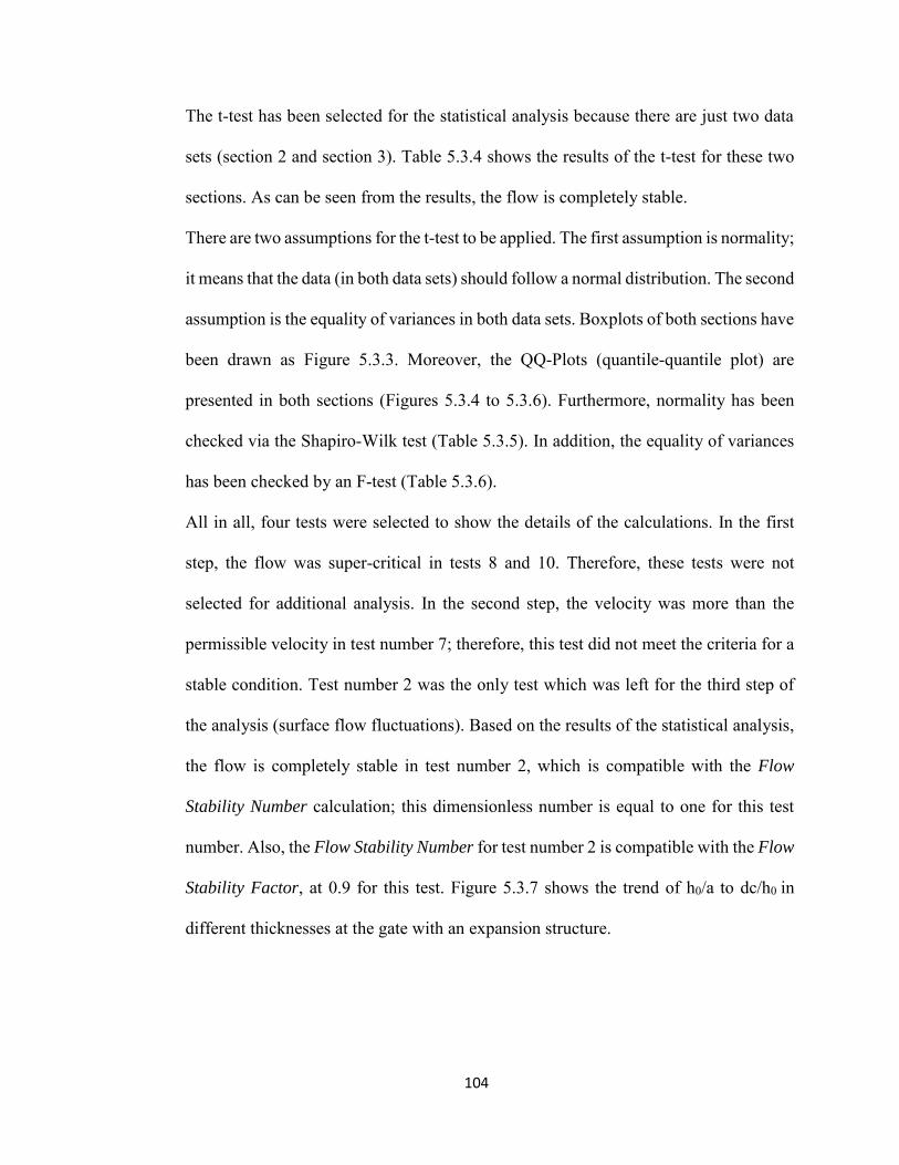
104
The t-test has been selected for the statistical analysis because there are just two data
sets (section 2 and section 3). Table 5.3.4 shows the results of the t-test for these two
sections. As can be seen from the results, the flow is completely stable.
There are two assumptions for the t-test to be applied. The first assumption is normality;
it means that the data (in both data sets) should follow a normal distribution. The second
assumption is the equality of variances in both data sets. Boxplots of both sections have
been drawn as Figure 5.3.3. Moreover, the QQ-Plots (quantile-quantile plot) are
presented in both sections (Figures 5.3.4 to 5.3.6). Furthermore, normality has been
checked via the Shapiro-Wilk test (Table 5.3.5). In addition, the equality of variances
has been checked by an F-test (Table 5.3.6).
All in all, four tests were selected to show the details of the calculations. In the first
step, the flow was super-critical in tests 8 and 10. Therefore, these tests were not
selected for additional analysis. In the second step, the velocity was more than the
permissible velocity in test number 7; therefore, this test did not meet the criteria for a
stable condition. Test number 2 was the only test which was left for the third step of
the analysis (surface flow fluctuations). Based on the results of the statistical analysis,
the flow is completely stable in test number 2, which is compatible with the Flow
Stability Number calculation; this dimensionless number is equal to one for this test
number. Also, the Flow Stability Number for test number 2 is compatible with the Flow
Stability Factor, at 0.9 for this test. Figure 5.3.7 shows the trend of h0/a to dc/h0 in
different thicknesses at the gate with an expansion structure.
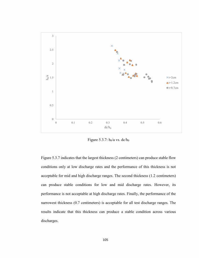
105
Figure 5.3.7: h0/a vs. dc/h0
Figure 5.3.7 indicates that the largest thickness (2 centimeters) can produce stable flow
conditions only at low discharge rates and the performance of this thickness is not
acceptable for mid and high discharge ranges. The second thickness (1.2 centimeters)
can produce stable conditions for low and mid discharge rates. However, its
performance is not acceptable at high discharge rates. Finally, the performance of the
narrowest thickness (0.7 centimeters) is acceptable for all test discharge ranges. The
results indicate that this thickness can produce a stable condition across various
discharges.
0
0.5
1
1.5
2
2.5
3
0 0.1 0.2 0.3 0.4 0.5 0.6
h 0/a
dc/h0
t=2cm
t=1.2cm
t=0.7cm
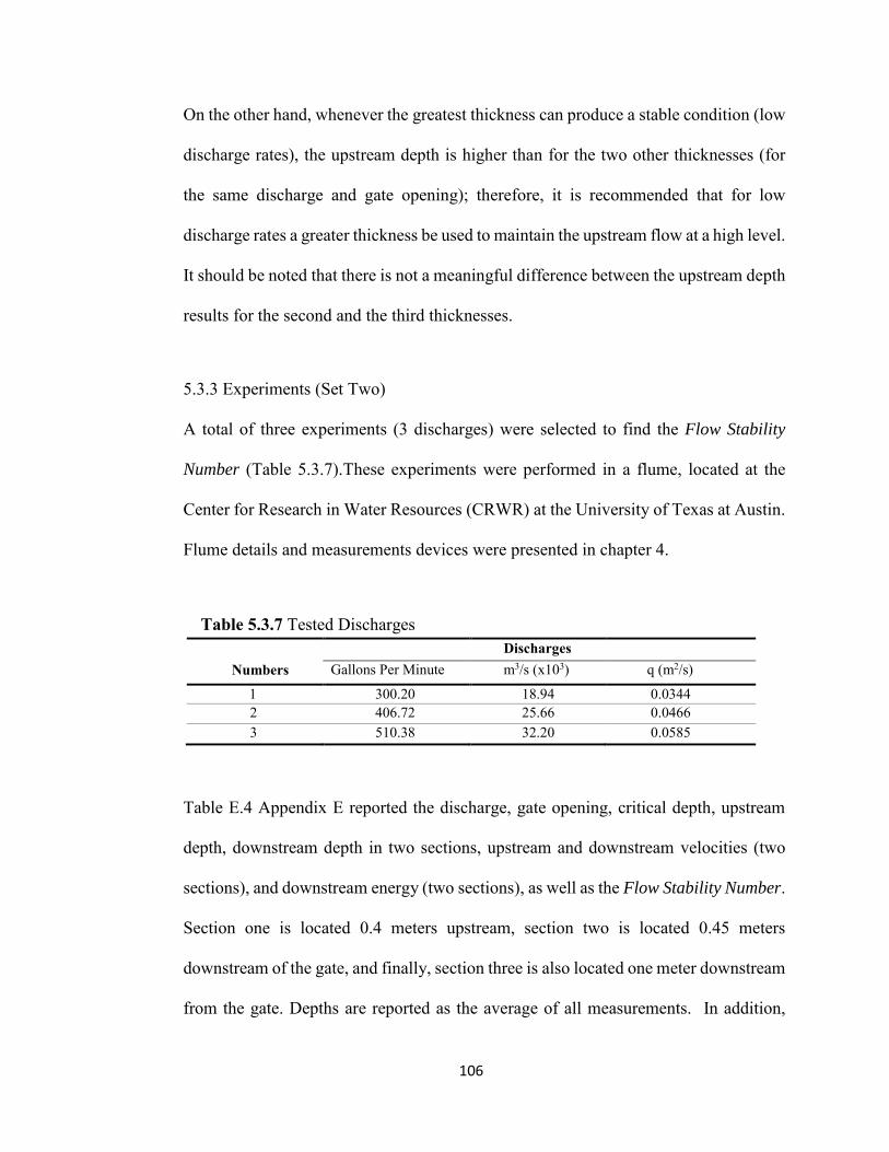
106
On the other hand, whenever the greatest thickness can produce a stable condition (low
discharge rates), the upstream depth is higher than for the two other thicknesses (for
the same discharge and gate opening); therefore, it is recommended that for low
discharge rates a greater thickness be used to maintain the upstream flow at a high level.
It should be noted that there is not a meaningful difference between the upstream depth
results for the second and the third thicknesses.
5.3.3 Experiments (Set Two)
A total of three experiments (3 discharges) were selected to find the Flow Stability
Number (Table 5.3.7).These experiments were performed in a flume, located at the
Center for Research in Water Resources (CRWR) at the University of Texas at Austin.
Flume details and measurements devices were presented in chapter 4.
Table 5.3.7 Tested Discharges
Discharges Numbers Gallons Per Minute m3/s (x103) q (m2/s)
1 300.20 18.94 0.0344 2 406.72 25.66 0.0466 3 510.38 32.20 0.0585
Table E.4 Appendix E reported the discharge, gate opening, critical depth, upstream
depth, downstream depth in two sections, upstream and downstream velocities (two
sections), and downstream energy (two sections), as well as the Flow Stability Number.
Section one is located 0.4 meters upstream, section two is located 0.45 meters
downstream of the gate, and finally, section three is also located one meter downstream
from the gate. Depths are reported as the average of all measurements. In addition,
107
Figures 5.3.8 (a) and (b) show the sediment transport and surface flow pattern in the
presence of a gate with an expansion.
Figure 5.3.8. (a): Sediment transport in the presence of a gate with an expansion
Figure 5.3.8. (b): Flow pattern in the presence of a gate with an expansion
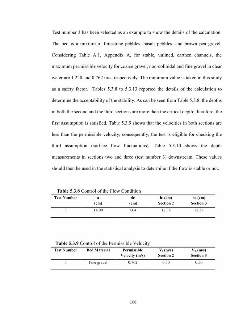
108
Test number 3 has been selected as an example to show the details of the calculation.
The bed is a mixture of limestone pebbles, basalt pebbles, and brown pea gravel.
Considering Table A.1, Appendix A, for stable, unlined, earthen channels, the
maximum permissible velocity for coarse gravel, non-colloidal and fine gravel in clear
water are 1.220 and 0.762 m/s, respectively. The minimum value is taken in this study
as a safety factor. Tables 5.3.8 to 5.3.13 reported the details of the calculation to
determine the acceptability of the stability. As can be seen from Table 5.3.8, the depths
in both the second and the third sections are more than the critical depth; therefore, the
first assumption is satisfied. Table 5.3.9 shows that the velocities in both sections are
less than the permissible velocity; consequently, the test is eligible for checking the
third assumption (surface flow fluctuations). Table 5.3.10 shows the depth
measurements in sections two and three (test number 3) downstream. These values
should then be used in the statistical analysis to determine if the flow is stable or not.
Table 5.3.8 Control of the Flow Condition Test Number a
(cm) dc
(cm) h1 (cm)
Section 2 h2 (cm)
Section 3
3 14.00 7.04 12.38 12.38
Table 5.3.9 Control of the Permissible Velocity Test Number Bed Material Permissible
Velocity (m/s) V1 (m/s)
Section 2 V2 (m/s)
Section 3
3 Fine gravel 0.762 0.50 0.50
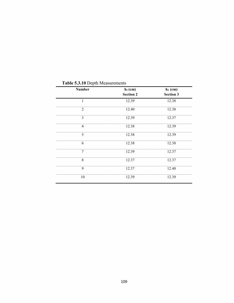
109
Table 5.3.10 Depth Measurements Number h1 (cm)
Section 2 h2 (cm)
Section 3
1 12.39 12.38
2 12.40 12.38
3 12.39 12.37
4 12.38 12.39
5 12.38 12.39
6 12.38 12.38
7 12.39 12.37
8 12.37 12.37
9 12.37 12.40
10 12.39 12.39
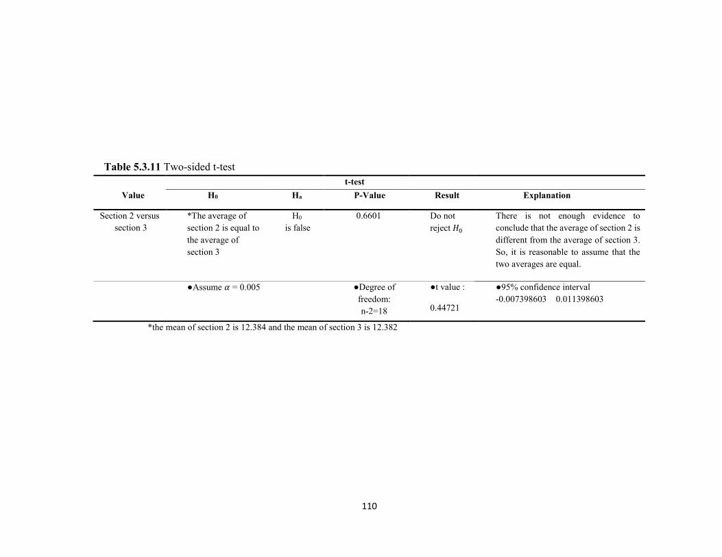
110
Table 5.3.11 Two-sided t-test t-test Value H0
Ha P-Value Result Explanation
Section 2 versus
section 3 *The average of section 2 is equal to the average of section 3
H0
is false 0.6601 Do not
reject 𝐻0
There is not enough evidence to conclude that the average of section 2 is different from the average of section 3. So, it is reasonable to assume that the two averages are equal.
●Assume 𝛼 = 0.005
●Degree of freedom: n-2=18
●t value :
0.44721
●95% confidence interval -0.007398603 0.011398603
*the mean of section 2 is 12.384 and the mean of section 3 is 12.382
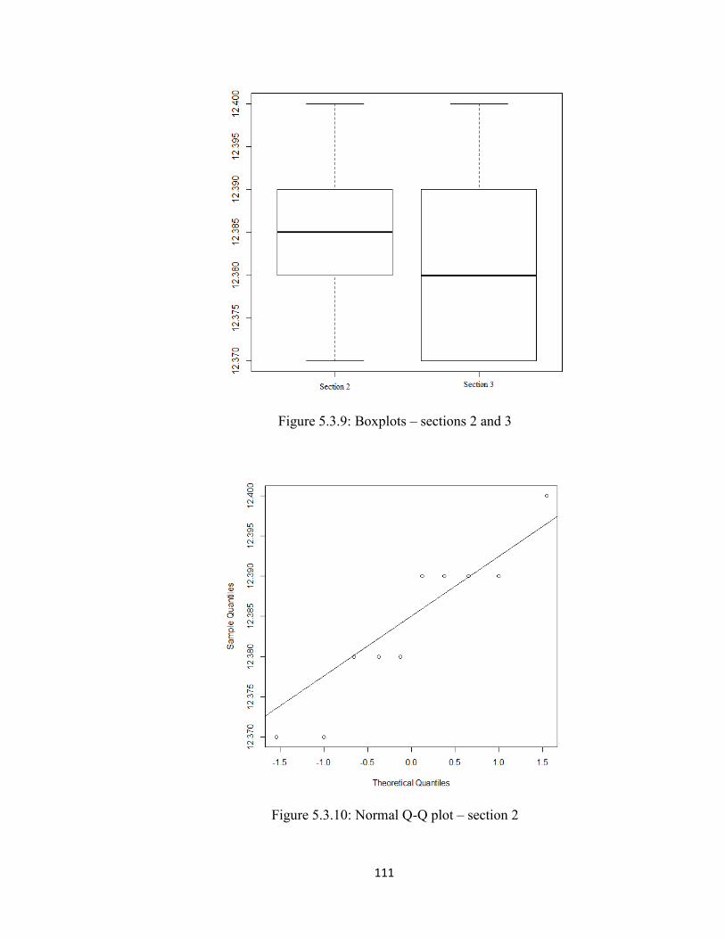
111
Figure 5.3.9: Boxplots – sections 2 and 3
Figure 5.3.10: Normal Q-Q plot – section 2
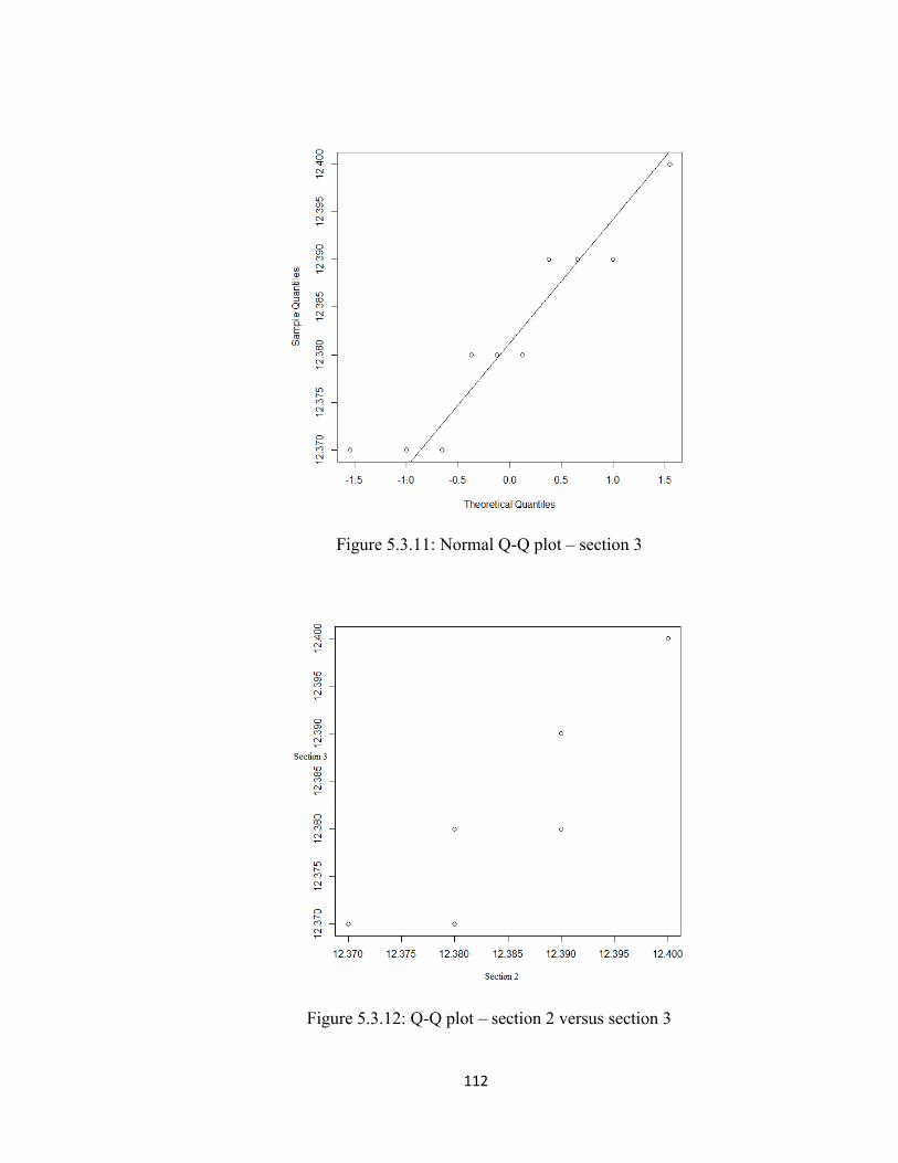
112
Figure 5.3.11: Normal Q-Q plot – section 3
Figure 5.3.12: Q-Q plot – section 2 versus section 3

113
Table 5.3.12 Check of Normality Shapiro-Wilk Test Value H0
Ha P-Value Result Explanation
h1 (cm)
Section 2 Data follows a normal distribution
H0
is false 0.2449 Do not
reject 𝐻0
Fail to reject the null hypothesis. So, it is reasonable to assume normality.
h2 (cm)
Section 3 Data follows a normal distribution
H0
is false
0.191 Do not reject 𝐻0
Fail to reject the null hypothesis. So, it is reasonable to assume normality.
Table 5.3.13 Check of the Equality of Variances F Test Value H0
Ha P-Value Result Explanation
Section 2 versus
section 3 The variance of section 2 is equal to the variance of section 3
H0
is false 0.8456 Do not
reject 𝐻0
Fail to reject the null hypothesis. So, it is reasonable to assume the equality of variances.
●Assume 𝛼 = 0.005
●Degree of freedom n-1=9
●95% confidence interval 0.2173376 3.5227449
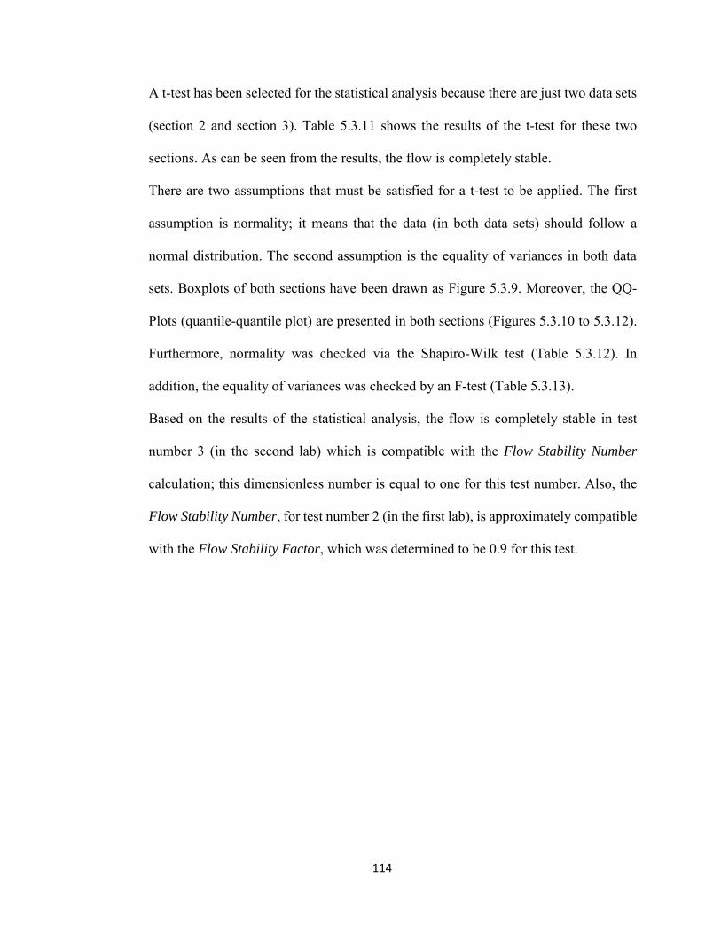
114
A t-test has been selected for the statistical analysis because there are just two data sets
(section 2 and section 3). Table 5.3.11 shows the results of the t-test for these two
sections. As can be seen from the results, the flow is completely stable.
There are two assumptions that must be satisfied for a t-test to be applied. The first
assumption is normality; it means that the data (in both data sets) should follow a
normal distribution. The second assumption is the equality of variances in both data
sets. Boxplots of both sections have been drawn as Figure 5.3.9. Moreover, the QQ-
Plots (quantile-quantile plot) are presented in both sections (Figures 5.3.10 to 5.3.12).
Furthermore, normality was checked via the Shapiro-Wilk test (Table 5.3.12). In
addition, the equality of variances was checked by an F-test (Table 5.3.13).
Based on the results of the statistical analysis, the flow is completely stable in test
number 3 (in the second lab) which is compatible with the Flow Stability Number
calculation; this dimensionless number is equal to one for this test number. Also, the
Flow Stability Number, for test number 2 (in the first lab), is approximately compatible
with the Flow Stability Factor, which was determined to be 0.9 for this test.
115
CHAPTER 5
RESULTS & DISCUSSION
SECTION 4
THE FLOW STABILITY NUMBER IN A GATE WITH
CONTRACTIONS
5.4.1 Introduction
The Flow Stability Number was calculated for vertical sluice gates in section 2 and a
gate with an expansion in section 3. In this section, a combination of gates with
contractions is considered as another type of hydraulic structure. The experiments were
conducted in two laboratories; the Fluid Mechanics Laboratory at Florida International
University and the Center for Research in Water Resources at the University of Texas
at Austin. Two laboratories were selected for this research to see the scale effect.
Moreover, sediment transport was considered in the second laboratory to find the
acceptable range of the Flow Stability Number.
Three thicknesses were considered in the first laboratory; 2 centimeters, 1.2
centimeters, and 0.7 centimeters to determine the effect of thickness on the Flow
Stability Number.
5.4.2 Experiments (Set One)
A total of 16 experiments, including five discharges (in one case, six discharges) and
three thicknesses, were selected from a gate with contraction results to find the Flow
116
Stability Number in the first laboratory.The experiments were conducted in a narrow
flume, located at the Fluid Mechanics Laboratory at the Civil and Environmental
Engineering Department of Florida International University. Flume details and
measurements devices were presented in chapter 4.
Six discharges were tested in this research and presented in Table 5.4.1, ranging from
low to high levels. For the narrowest thickness, six tests were performed. Determining
the effect of thickness on the Flow Stability Number for each discharge was the purpose
of this study. The optimum gate opening happens when the flow condition is stable
downstream of the hydraulic structure.
The Flow Stability Number was defined in chapter 4, based on the Fuzzy Concept in
sub-critical flow, to classify the downstream flow condition. This dimensionless
number is defined based on total energy. Velocity and depth were measured to calculate
energy. In each test, measurements were performed in four sections; one section
upstream of the hydraulic structure, one inside the structure, and two downstream of
the structure.
Tables F.1 to F.3 Appendix F reported the discharge, gate opening, critical depth,
upstream depth, downstream depth in two sections, upstream and downstream velocity
(two sections), and downstream energy (two sections), as well as the Flow Stability
Number for a gate with contractions with different thicknesses. The results of the
section inside the hydraulic structure are not reported in these; therefore, section one is
located upstream, section two is located immediately after the hydraulic structure, and
finally, section three is also located downstream from section two at the beginning of
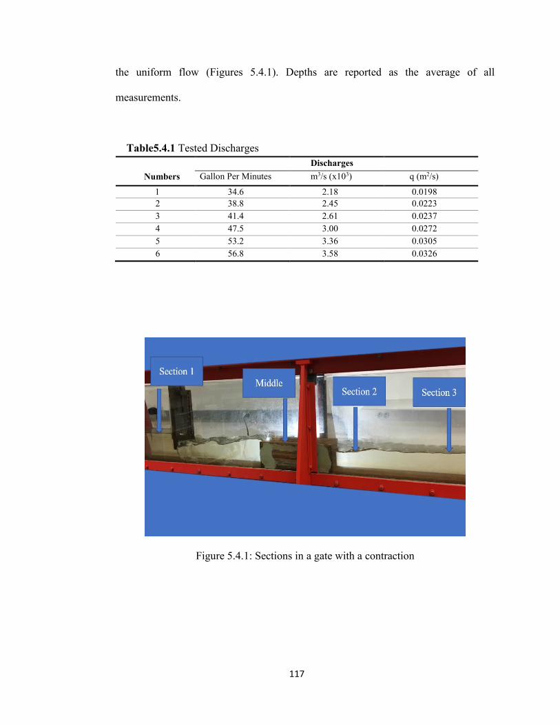
117
the uniform flow (Figures 5.4.1). Depths are reported as the average of all
measurements.
Table5.4.1 Tested Discharges Discharges Numbers Gallon Per Minutes
(GPM)
m3/s (x103) q (m2/s)
1 34.6 2.18 0.0198 2 38.8 2.45 0.0223 3 41.4 2.61 0.0237 4 47.5 3.00 0.0272 5 53.2 3.36 0.0305 6 56.8 3.58 0.0326
Figure 5.4.1: Sections in a gate with a contraction
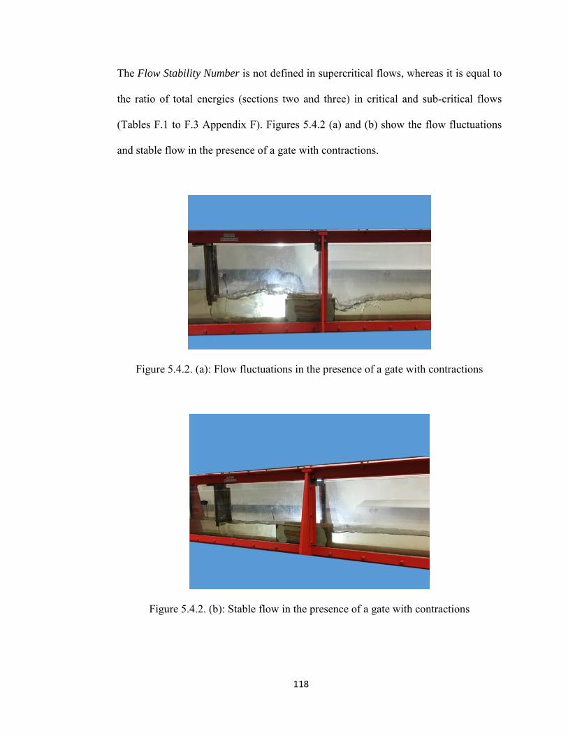
118
The Flow Stability Number is not defined in supercritical flows, whereas it is equal to
the ratio of total energies (sections two and three) in critical and sub-critical flows
(Tables F.1 to F.3 Appendix F). Figures 5.4.2 (a) and (b) show the flow fluctuations
and stable flow in the presence of a gate with contractions.
Figure 5.4.2. (a): Flow fluctuations in the presence of a gate with contractions
Figure 5.4.2. (b): Stable flow in the presence of a gate with contractions
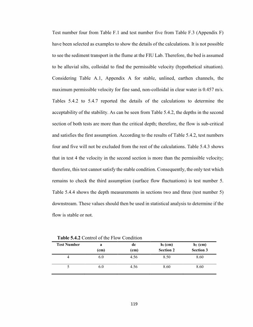
119
Test number four from Table F.1 and test number five from Table F.3 (Appendix F)
have been selected as examples to show the details of the calculations. It is not possible
to see the sediment transport in the flume at the FIU Lab. Therefore, the bed is assumed
to be alluvial silts, colloidal to find the permissible velocity (hypothetical situation).
Considering Table A.1, Appendix A for stable, unlined, earthen channels, the
maximum permissible velocity for fine sand, non-colloidal in clear water is 0.457 m/s.
Tables 5.4.2 to 5.4.7 reported the details of the calculations to determine the
acceptability of the stability. As can be seen from Table 5.4.2, the depths in the second
section of both tests are more than the critical depth; therefore, the flow is sub-critical
and satisfies the first assumption. According to the results of Table 5.4.2, test numbers
four and five will not be excluded from the rest of the calculations. Table 5.4.3 shows
that in test 4 the velocity in the second section is more than the permissible velocity;
therefore, this test cannot satisfy the stable condition. Consequently, the only test which
remains to check the third assumption (surface flow fluctuations) is test number 5.
Table 5.4.4 shows the depth measurements in sections two and three (test number 5)
downstream. These values should then be used in statistical analysis to determine if the
flow is stable or not.
Table 5.4.2 Control of the Flow Condition Test Number a
(cm) dc
(cm) h1 (cm)
Section 2 h2 (cm)
Section 3
4 6.0 4.56 8.50 8.60
5 6.0 4.56 8.60 8.60
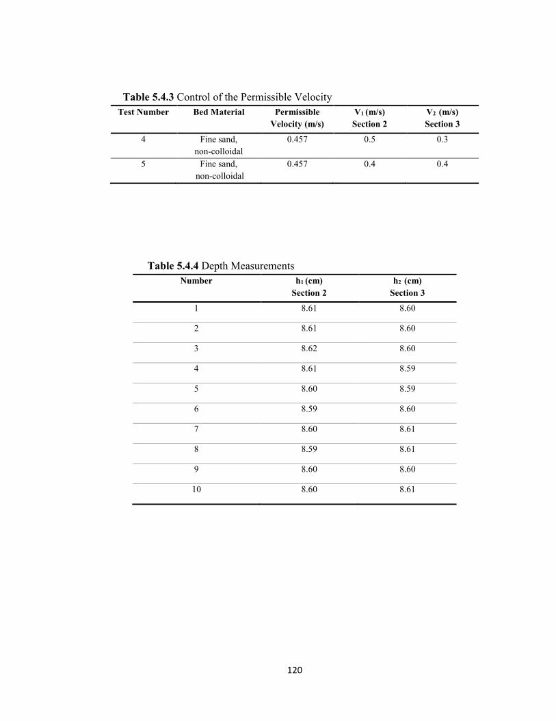
120
Table 5.4.3 Control of the Permissible Velocity Test Number Bed Material Permissible
Velocity (m/s) V1 (m/s)
Section 2 V2 (m/s)
Section 3
4 Fine sand, non-colloidal
0.457 0.5 0.3
5 Fine sand, non-colloidal
0.457 0.4 0.4
Table 5.4.4 Depth Measurements Number h1 (cm)
Section 2 h2 (cm)
Section 3
1 8.61 8.60
2 8.61 8.60
3 8.62 8.60
4 8.61 8.59
5 8.60 8.59
6 8.59 8.60
7 8.60 8.61
8 8.59 8.61
9 8.60 8.60
10 8.60 8.61
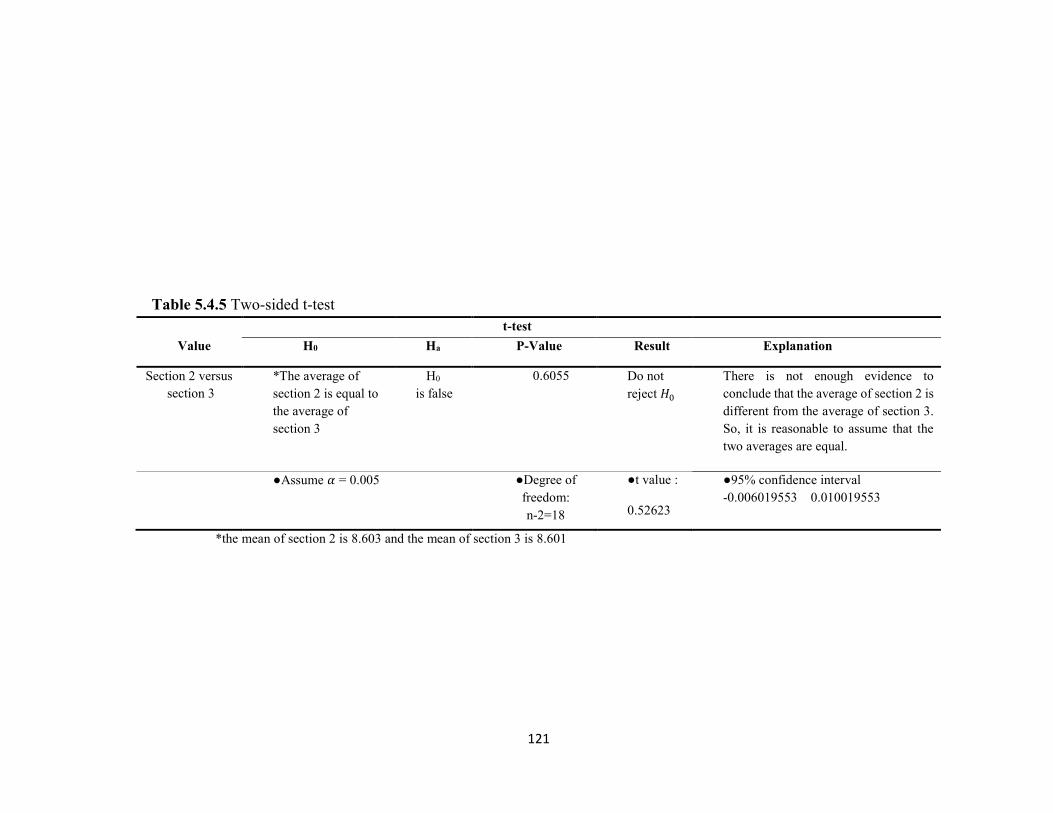
121
Table 5.4.5 Two-sided t-test t-test Value H0
Ha P-Value Result Explanation
Section 2 versus
section 3 *The average of section 2 is equal to the average of section 3
H0
is false 0.6055 Do not
reject 𝐻0
There is not enough evidence to conclude that the average of section 2 is different from the average of section 3. So, it is reasonable to assume that the two averages are equal.
●Assume 𝛼 = 0.005
●Degree of freedom: n-2=18
●t value :
0.52623
●95% confidence interval -0.006019553 0.010019553
*the mean of section 2 is 8.603 and the mean of section 3 is 8.601
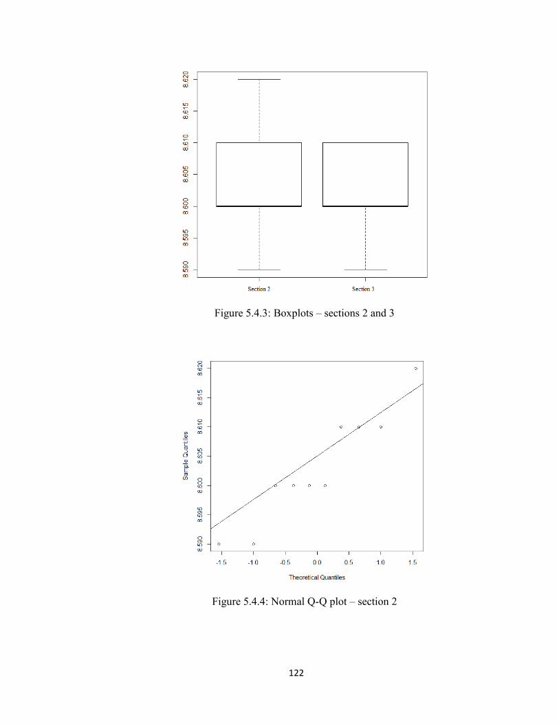
122
Figure 5.4.3: Boxplots – sections 2 and 3
Figure 5.4.4: Normal Q-Q plot – section 2
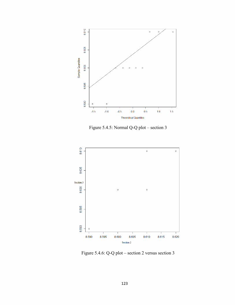
123
Figure 5.4.5: Normal Q-Q plot – section 3
Figure 5.4.6: Q-Q plot – section 2 versus section 3
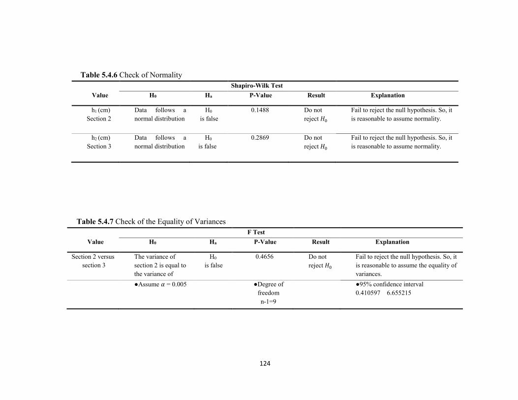
124
Table 5.4.6 Check of Normality Shapiro-Wilk Test Value H0
Ha P-Value Result Explanation
h1 (cm)
Section 2 Data follows a normal distribution
H0
is false 0.1488 Do not
reject 𝐻0
Fail to reject the null hypothesis. So, it is reasonable to assume normality.
h2 (cm)
Section 3 Data follows a normal distribution
H0
is false
0.2869 Do not reject 𝐻0
Fail to reject the null hypothesis. So, it is reasonable to assume normality.
Table 5.4.7 Check of the Equality of Variances F Test Value H0
Ha P-Value Result Explanation
Section 2 versus
section 3 The variance of section 2 is equal to the variance of section 3
H0
is false 0.4656 Do not
reject 𝐻0
Fail to reject the null hypothesis. So, it is reasonable to assume the equality of variances.
●Assume 𝛼 = 0.005
●Degree of freedom n-1=9
●95% confidence interval 0.410597 6.655215
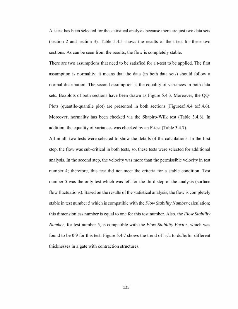
125
A t-test has been selected for the statistical analysis because there are just two data sets
(section 2 and section 3). Table 5.4.5 shows the results of the t-test for these two
sections. As can be seen from the results, the flow is completely stable.
There are two assumptions that need to be satisfied for a t-test to be applied. The first
assumption is normality; it means that the data (in both data sets) should follow a
normal distribution. The second assumption is the equality of variances in both data
sets. Boxplots of both sections have been drawn as Figure 5.4.3. Moreover, the QQ-
Plots (quantile-quantile plot) are presented in both sections (Figures5.4.4 to5.4.6).
Moreover, normality has been checked via the Shapiro-Wilk test (Table 3.4.6). In
addition, the equality of variances was checked by an F-test (Table 3.4.7).
All in all, two tests were selected to show the details of the calculations. In the first
step, the flow was sub-critical in both tests, so, these tests were selected for additional
analysis. In the second step, the velocity was more than the permissible velocity in test
number 4; therefore, this test did not meet the criteria for a stable condition. Test
number 5 was the only test which was left for the third step of the analysis (surface
flow fluctuations). Based on the results of the statistical analysis, the flow is completely
stable in test number 5 which is compatible with the Flow Stability Number calculation;
this dimensionless number is equal to one for this test number. Also, the Flow Stability
Number, for test number 5, is compatible with the Flow Stability Factor, which was
found to be 0.9 for this test. Figure 5.4.7 shows the trend of h0/a to dc/h0 for different
thicknesses in a gate with contraction structures.
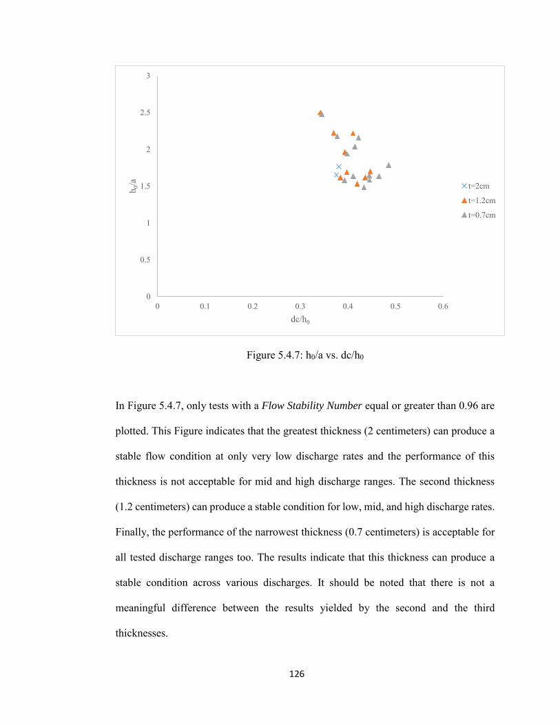
126
Figure 5.4.7: h0/a vs. dc/h0
In Figure 5.4.7, only tests with a Flow Stability Number equal or greater than 0.96 are
plotted. This Figure indicates that the greatest thickness (2 centimeters) can produce a
stable flow condition at only very low discharge rates and the performance of this
thickness is not acceptable for mid and high discharge ranges. The second thickness
(1.2 centimeters) can produce a stable condition for low, mid, and high discharge rates.
Finally, the performance of the narrowest thickness (0.7 centimeters) is acceptable for
all tested discharge ranges too. The results indicate that this thickness can produce a
stable condition across various discharges. It should be noted that there is not a
meaningful difference between the results yielded by the second and the third
thicknesses.
0
0.5
1
1.5
2
2.5
3
0 0.1 0.2 0.3 0.4 0.5 0.6
h 0/a
dc/h0
t=2cm
t=1.2cm
t=0.7cm
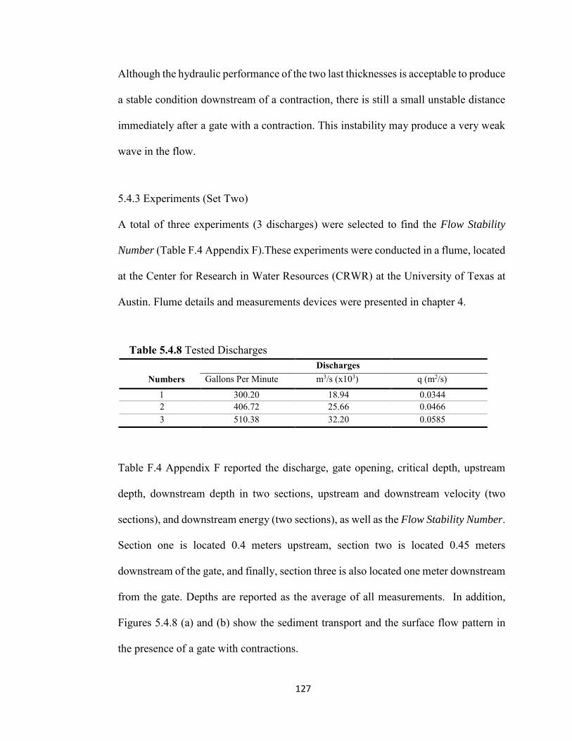
127
Although the hydraulic performance of the two last thicknesses is acceptable to produce
a stable condition downstream of a contraction, there is still a small unstable distance
immediately after a gate with a contraction. This instability may produce a very weak
wave in the flow.
5.4.3 Experiments (Set Two)
A total of three experiments (3 discharges) were selected to find the Flow Stability
Number (Table F.4 Appendix F).These experiments were conducted in a flume, located
at the Center for Research in Water Resources (CRWR) at the University of Texas at
Austin. Flume details and measurements devices were presented in chapter 4.
Table 5.4.8 Tested Discharges
Discharges Numbers Gallons Per Minute m3/s (x103) q (m2/s)
1 300.20 18.94 0.0344 2 406.72 25.66 0.0466 3 510.38 32.20 0.0585
Table F.4 Appendix F reported the discharge, gate opening, critical depth, upstream
depth, downstream depth in two sections, upstream and downstream velocity (two
sections), and downstream energy (two sections), as well as the Flow Stability Number.
Section one is located 0.4 meters upstream, section two is located 0.45 meters
downstream of the gate, and finally, section three is also located one meter downstream
from the gate. Depths are reported as the average of all measurements. In addition,
Figures 5.4.8 (a) and (b) show the sediment transport and the surface flow pattern in
the presence of a gate with contractions.
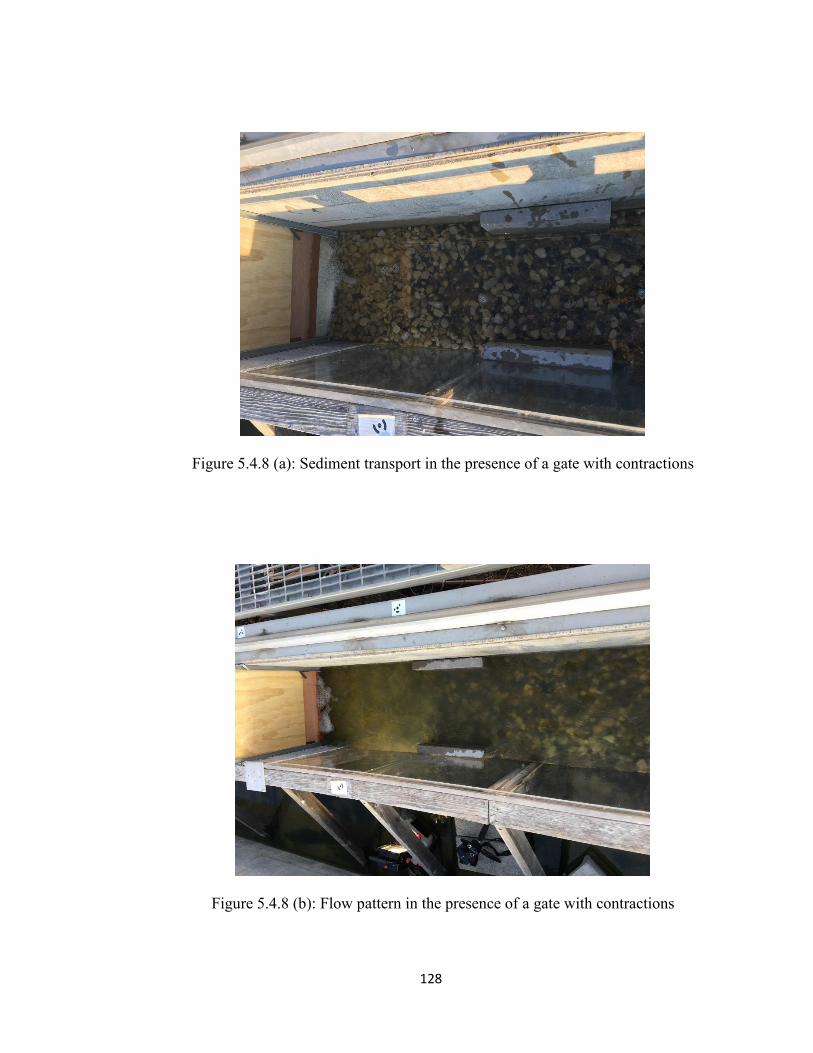
128
Figure 5.4.8 (a): Sediment transport in the presence of a gate with contractions
Figure 5.4.8 (b): Flow pattern in the presence of a gate with contractions
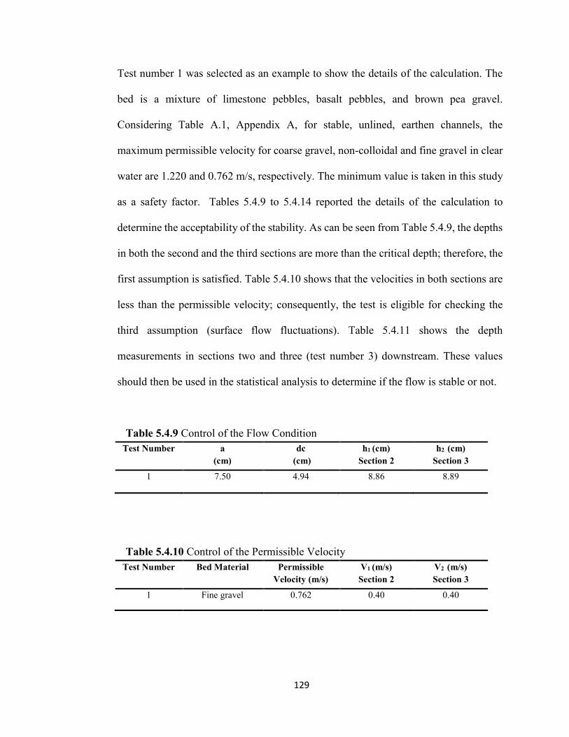
129
Test number 1 was selected as an example to show the details of the calculation. The
bed is a mixture of limestone pebbles, basalt pebbles, and brown pea gravel.
Considering Table A.1, Appendix A, for stable, unlined, earthen channels, the
maximum permissible velocity for coarse gravel, non-colloidal and fine gravel in clear
water are 1.220 and 0.762 m/s, respectively. The minimum value is taken in this study
as a safety factor. Tables 5.4.9 to 5.4.14 reported the details of the calculation to
determine the acceptability of the stability. As can be seen from Table 5.4.9, the depths
in both the second and the third sections are more than the critical depth; therefore, the
first assumption is satisfied. Table 5.4.10 shows that the velocities in both sections are
less than the permissible velocity; consequently, the test is eligible for checking the
third assumption (surface flow fluctuations). Table 5.4.11 shows the depth
measurements in sections two and three (test number 3) downstream. These values
should then be used in the statistical analysis to determine if the flow is stable or not.
Table 5.4.9 Control of the Flow Condition Test Number a
(cm) dc
(cm) h1 (cm)
Section 2 h2 (cm)
Section 3
1 7.50 4.94 8.86 8.89
Table 5.4.10 Control of the Permissible Velocity Test Number Bed Material Permissible
Velocity (m/s) V1 (m/s)
Section 2 V2 (m/s)
Section 3
1 Fine gravel 0.762 0.40 0.40
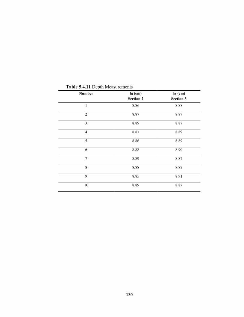
130
Table 5.4.11 Depth Measurements Number h1 (cm)
Section 2 h2 (cm)
Section 3
1 8.86 8.88
2 8.87 8.87
3 8.89 8.87
4 8.87 8.89
5 8.86 8.89
6 8.88 8.90
7 8.89 8.87
8 8.88 8.89
9 8.85 8.91
10 8.89 8.87
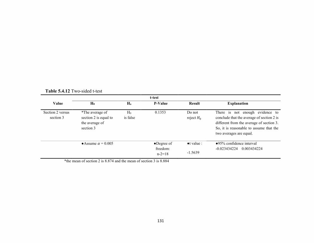
131
Table 5.4.12 Two-sided t-test t-test Value H0
Ha P-Value Result Explanation
Section 2 versus
section 3 *The average of section 2 is equal to the average of section 3
H0
is false 0.1353 Do not
reject 𝐻0
There is not enough evidence to conclude that the average of section 2 is different from the average of section 3. So, it is reasonable to assume that the two averages are equal.
●Assume 𝛼 = 0.005
●Degree of freedom: n-2=18
●t value :
-1.5639
●95% confidence interval -0.023434224 0.003434224
*the mean of section 2 is 8.874 and the mean of section 3 is 8.884
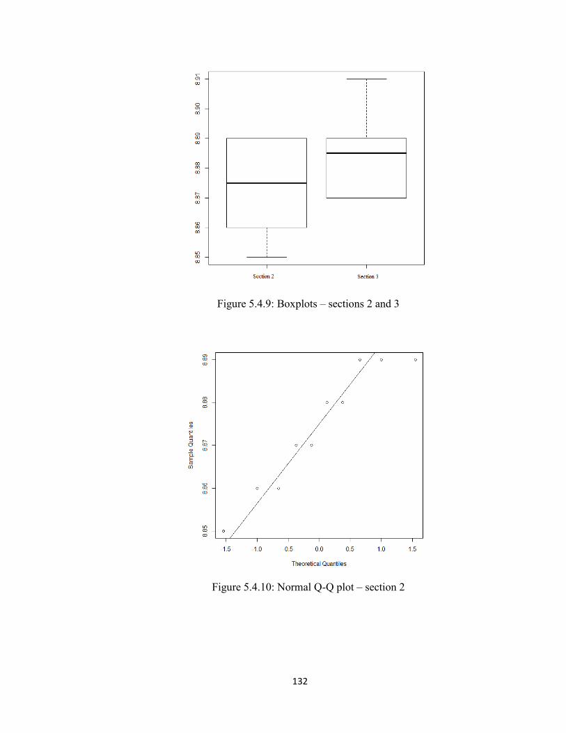
132
Figure 5.4.9: Boxplots – sections 2 and 3
Figure 5.4.10: Normal Q-Q plot – section 2
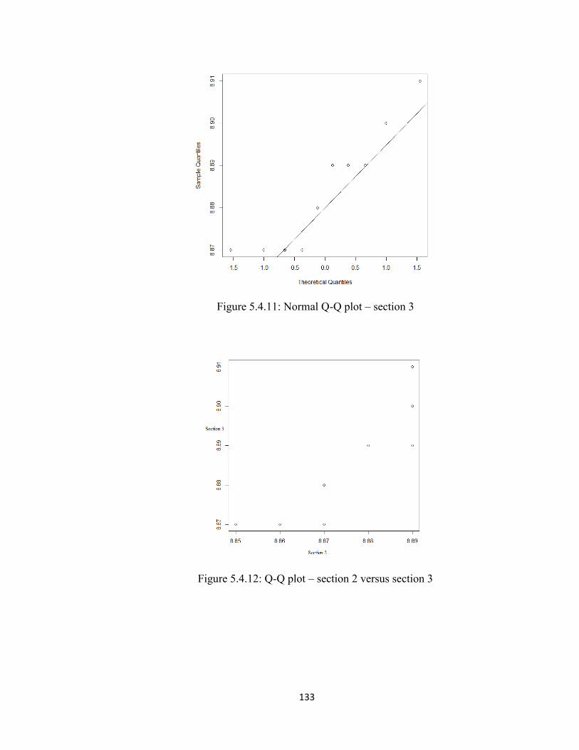
133
Figure 5.4.11: Normal Q-Q plot – section 3
Figure 5.4.12: Q-Q plot – section 2 versus section 3
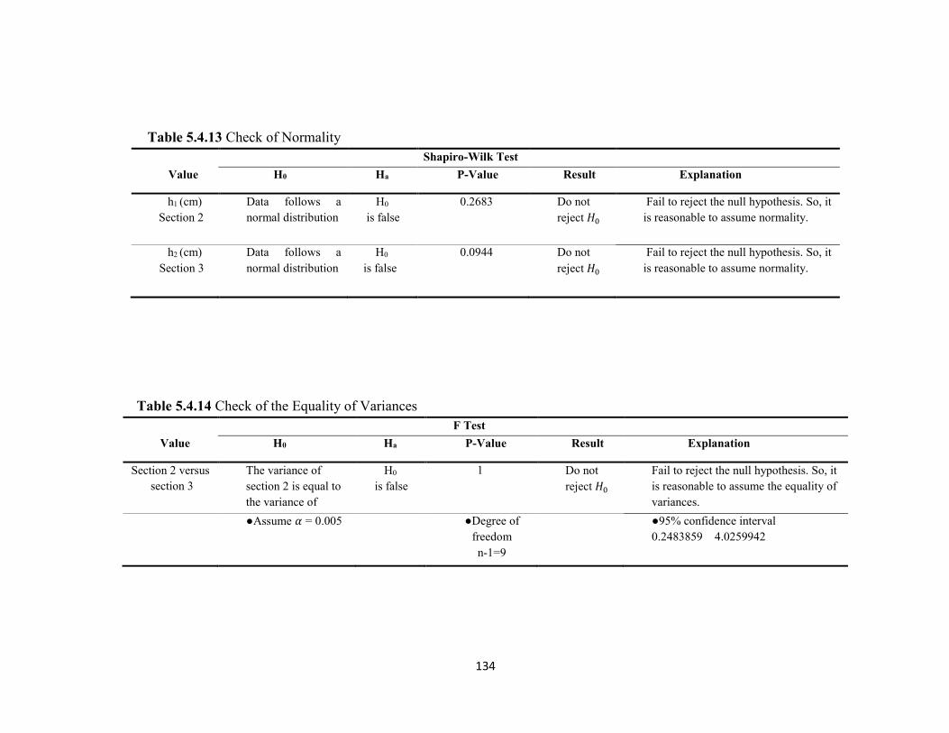
134
Table 5.4.13 Check of Normality Shapiro-Wilk Test Value H0
Ha P-Value Result Explanation
h1 (cm)
Section 2 Data follows a normal distribution
H0
is false 0.2683 Do not
reject 𝐻0
Fail to reject the null hypothesis. So, it is reasonable to assume normality.
h2 (cm)
Section 3 Data follows a normal distribution
H0
is false
0.0944 Do not reject 𝐻0
Fail to reject the null hypothesis. So, it is reasonable to assume normality.
Table 5.4.14 Check of the Equality of Variances F Test Value H0
Ha P-Value Result Explanation
Section 2 versus
section 3 The variance of section 2 is equal to the variance of section 3
H0
is false 1 Do not
reject 𝐻0
Fail to reject the null hypothesis. So, it is reasonable to assume the equality of variances.
●Assume 𝛼 = 0.005
●Degree of freedom n-1=9
●95% confidence interval 0.2483859 4.0259942
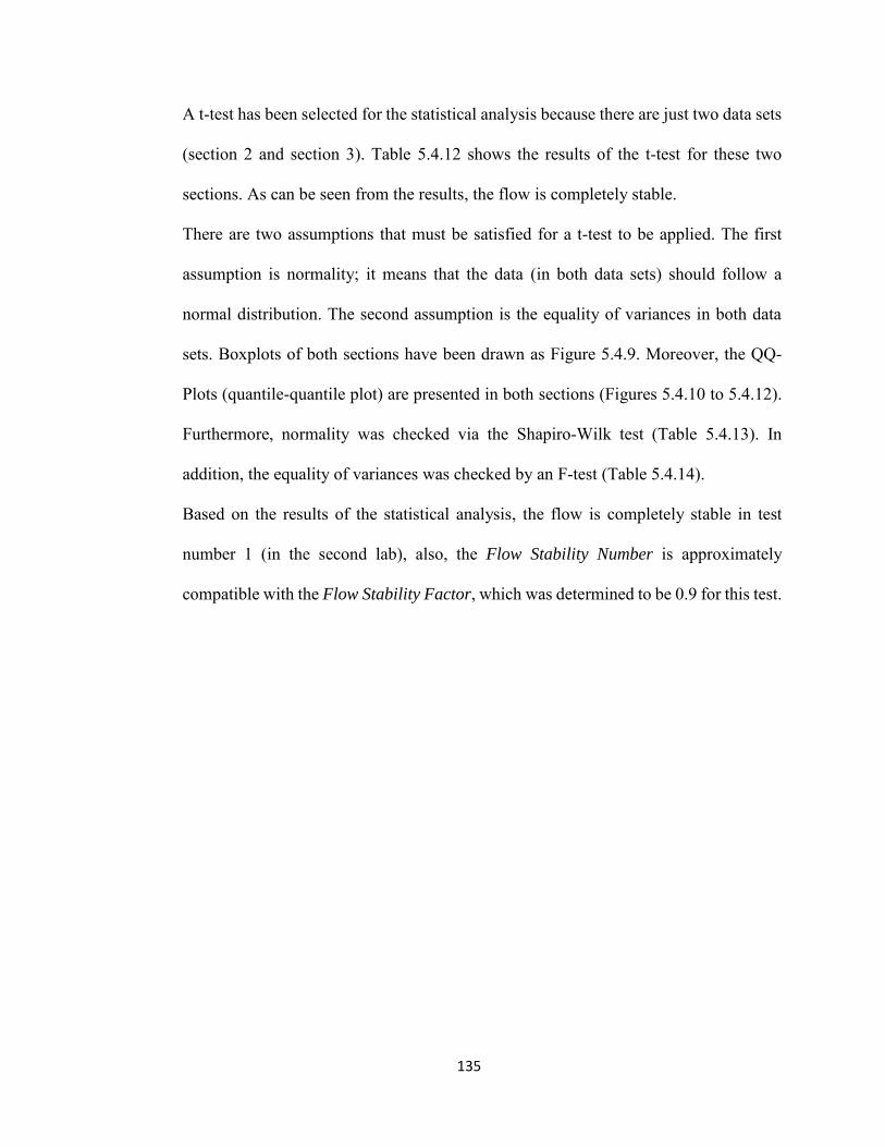
135
A t-test has been selected for the statistical analysis because there are just two data sets
(section 2 and section 3). Table 5.4.12 shows the results of the t-test for these two
sections. As can be seen from the results, the flow is completely stable.
There are two assumptions that must be satisfied for a t-test to be applied. The first
assumption is normality; it means that the data (in both data sets) should follow a
normal distribution. The second assumption is the equality of variances in both data
sets. Boxplots of both sections have been drawn as Figure 5.4.9. Moreover, the QQ-
Plots (quantile-quantile plot) are presented in both sections (Figures 5.4.10 to 5.4.12).
Furthermore, normality was checked via the Shapiro-Wilk test (Table 5.4.13). In
addition, the equality of variances was checked by an F-test (Table 5.4.14).
Based on the results of the statistical analysis, the flow is completely stable in test
number 1 (in the second lab), also, the Flow Stability Number is approximately
compatible with the Flow Stability Factor, which was determined to be 0.9 for this test.
136
CHAPTER 5
RESULTS & DISCUSSION
SECTION 5
COMPARISON OF THE RESULTS OF A GATE, A GATE WITH
EXPANSION, AND A GATE WITH CONTRACTION
5.5.1 Introduction
This research introduced the Flow Stability Factor as a new flow classification method,
which works based on the Fuzzy Concept and can be used downstream of hydraulic
structures. In addition, the Flow Stability Number — a ratio of energy in two sections
— was introduced as a new dimensionless number. These sections are located
downstream of the hydraulic structures. Due to the novelty of the Flow Stability Factor,
as well as the Flow Stability Number, the results can not be compared with any previous
studies. Therefore, in this section, the results of hydraulic structures which were used
in this research were compared with each other. These hydraulic structures include a
gate and a gate with expansion, as well as a gate with contraction. This section has four
parts, not including the introduction. In the first part, the outcomes of the Flow Stability
Factor and Flow Stability Number are compared with some experiments on a gate, a
gate with expansion, and a gate with contraction. The second part shows the
comparison between three hydraulic structures. In this part, the smallest thickness for
a gate with expansion and a gate with contraction which are represented as the best
results for these structures were compared with the results of gates in a dimensionless
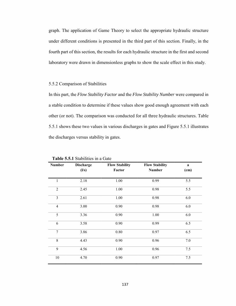
137
graph. The application of Game Theory to select the appropriate hydraulic structure
under different conditions is presented in the third part of this section. Finally, in the
fourth part of this section, the results for each hydraulic structure in the first and second
laboratory were drawn in dimensionless graphs to show the scale effect in this study.
5.5.2 Comparison of Stabilities
In this part, the Flow Stability Factor and the Flow Stability Number were compared in
a stable condition to determine if these values show good enough agreement with each
other (or not). The comparison was conducted for all three hydraulic structures. Table
5.5.1 shows these two values in various discharges in gates and Figure 5.5.1 illustrates
the discharges versus stability in gates.
Table 5.5.1 Stabilities in a Gate Number Discharge
(l/s) Flow Stability
Factor Flow Stability
Number a
(cm)
1 2.18 1.00 0.99 5.5
2 2.45 1.00 0.98 5.5
3 2.61 1.00 0.98 6.0
4 3.00 0.90 0.98 6.0
5 3.36 0.90 1.00 6.0
6 3.58 0.90 0.99 6.5
7 3.86 0.80 0.97 6.5
8 4.43 0.90 0.96 7.0
9 4.56 1.00 0.96 7.5
10 4.70 0.90 0.97 7.5
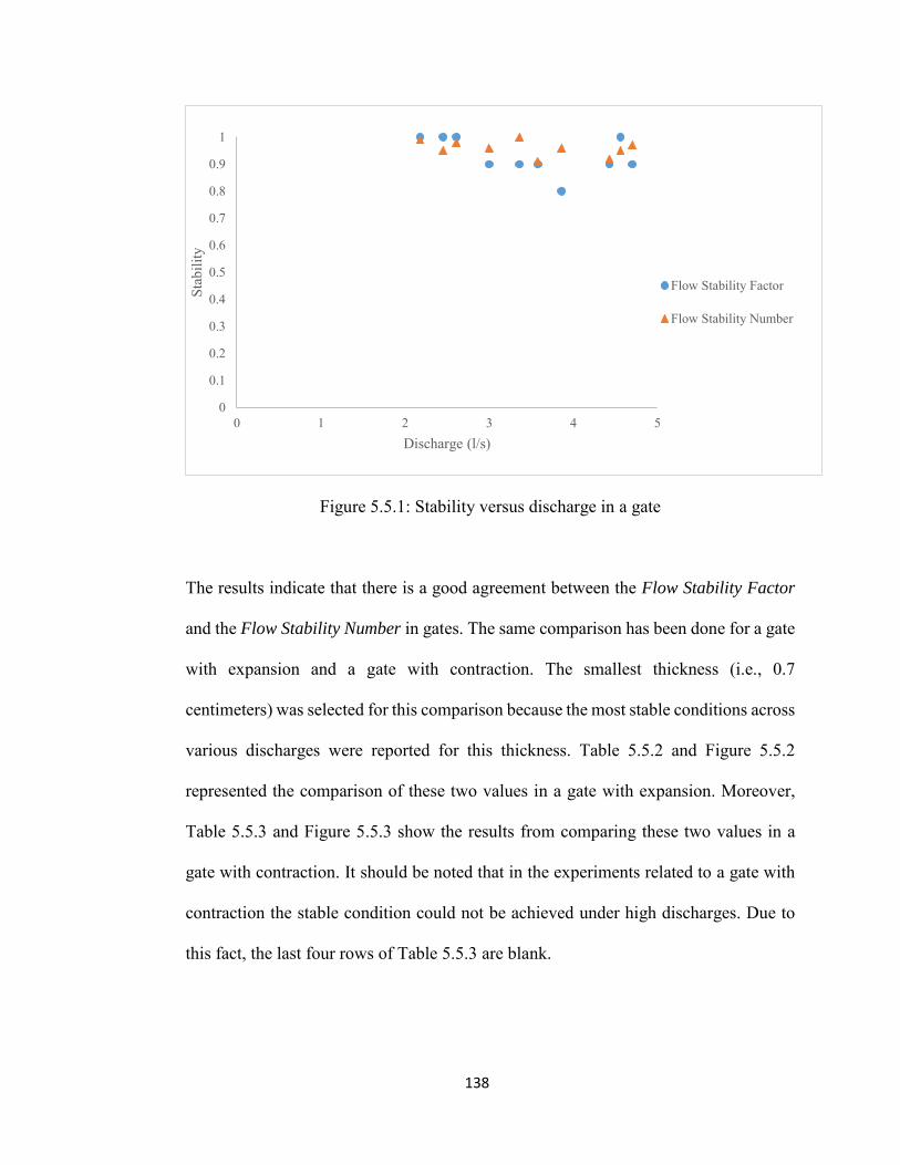
138
Figure 5.5.1: Stability versus discharge in a gate
The results indicate that there is a good agreement between the Flow Stability Factor
and the Flow Stability Number in gates. The same comparison has been done for a gate
with expansion and a gate with contraction. The smallest thickness (i.e., 0.7
centimeters) was selected for this comparison because the most stable conditions across
various discharges were reported for this thickness. Table 5.5.2 and Figure 5.5.2
represented the comparison of these two values in a gate with expansion. Moreover,
Table 5.5.3 and Figure 5.5.3 show the results from comparing these two values in a
gate with contraction. It should be noted that in the experiments related to a gate with
contraction the stable condition could not be achieved under high discharges. Due to
this fact, the last four rows of Table 5.5.3 are blank.
0
0.1
0.2
0.3
0.4
0.5
0.6
0.7
0.8
0.9
1
0 1 2 3 4 5
Stab
ility
Discharge (l/s)
Flow Stability Factor
Flow Stability Number
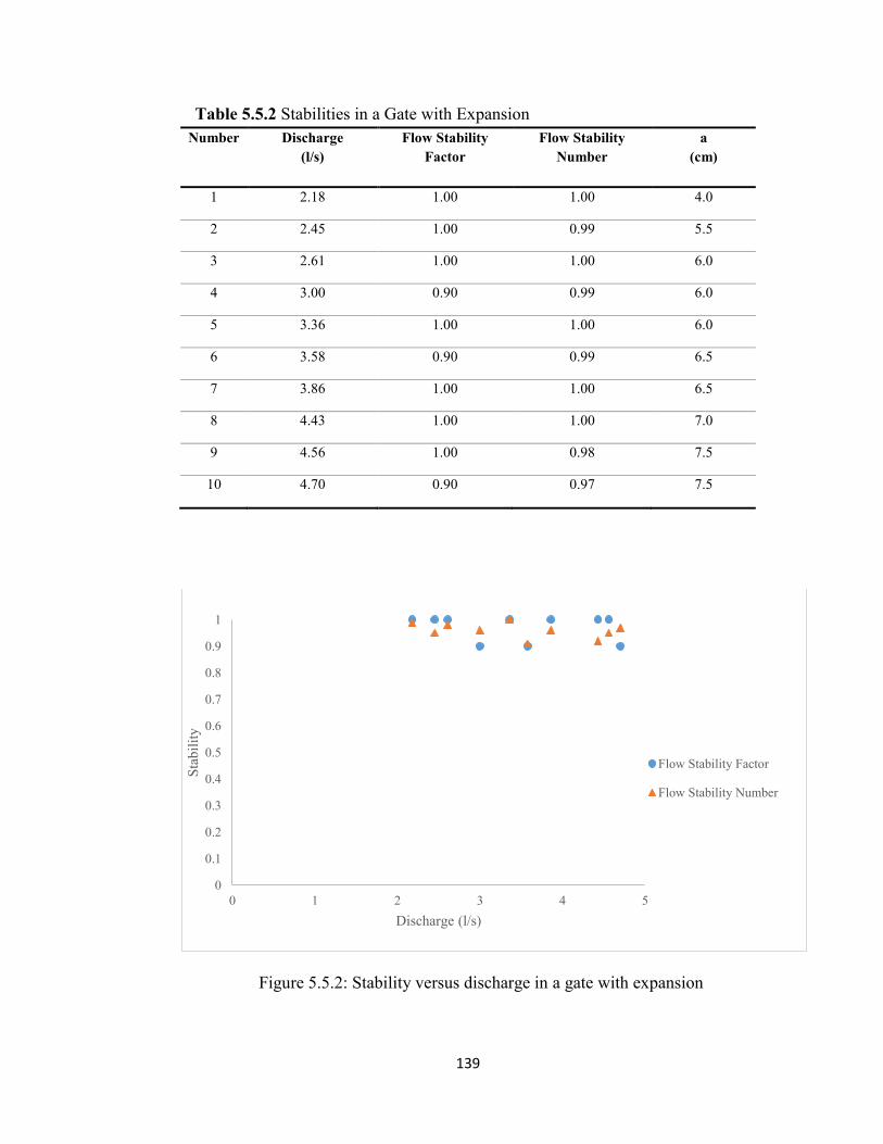
139
Table 5.5.2 Stabilities in a Gate with Expansion Number Discharge
(l/s) Flow Stability
Factor Flow Stability
Number a
(cm)
1 2.18 1.00 1.00 4.0
2 2.45 1.00 0.99 5.5
3 2.61 1.00 1.00 6.0
4 3.00 0.90 0.99 6.0
5 3.36 1.00 1.00 6.0
6 3.58 0.90 0.99 6.5
7 3.86 1.00 1.00 6.5
8 4.43 1.00 1.00 7.0
9 4.56 1.00 0.98 7.5
10 4.70 0.90 0.97 7.5
Figure 5.5.2: Stability versus discharge in a gate with expansion
0
0.1
0.2
0.3
0.4
0.5
0.6
0.7
0.8
0.9
1
0 1 2 3 4 5
Stab
ility
Discharge (l/s)
Flow Stability Factor
Flow Stability Number
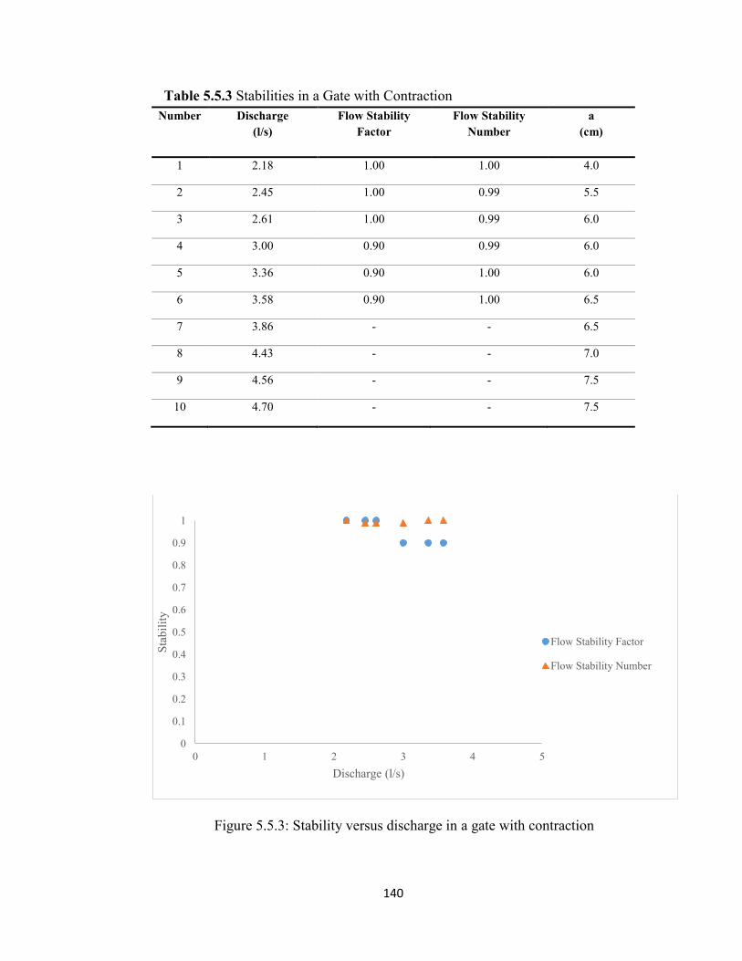
140
Table 5.5.3 Stabilities in a Gate with Contraction Number Discharge
(l/s) Flow Stability
Factor Flow Stability
Number a
(cm)
1 2.18 1.00 1.00 4.0
2 2.45 1.00 0.99 5.5
3 2.61 1.00 0.99 6.0
4 3.00 0.90 0.99 6.0
5 3.36 0.90 1.00 6.0
6 3.58 0.90 1.00 6.5
7 3.86 - - 6.5
8 4.43 - - 7.0
9 4.56 - - 7.5
10 4.70 - - 7.5
Figure 5.5.3: Stability versus discharge in a gate with contraction
0
0.1
0.2
0.3
0.4
0.5
0.6
0.7
0.8
0.9
1
0 1 2 3 4 5
Stab
ility
Discharge (l/s)
Flow Stability Factor
Flow Stability Number
141
It can be inferred from the results that the Flow Stability Factor and Flow Stability
Number are in good agreement with each other for all three tested hydraulic structures.
The depth and velocity measures are needed to calculate the Flow Stability Number.
However, the determination of the Flow Stability Factor is based on visual engineering
judgment. Therefore, Flow Stability Factor, instead of the Flow Stability Number, can
be determined and used in practical works with a high degree of reliability without any
measurements and calculations to find the flow stability condition downstream of
hydraulic structures. Furthermore, the results indicate that the hydraulic gate with a
contraction structure does not have a good hydraulic performance, and it is not able to
establish a stable condition under high discharges.
5.5.3 Comparison of a Gate, a Gate with Expansion, and a Gate with Contraction
The performance of all three tested hydraulic structures, including a gate, a gate with
expansion, and a gate with contraction, were compared based on the graph using
dimensionless numbers. Some researchers developed and presented different
dimensionless numbers in sluice gates [5, 114, 89]. Bijankhan et al. [5] developed and
used dc/a and h0/a in his research to establish a new stage-discharge relationship in
radial gates. Ferro [114] also developed and used the same dimensionless numbers to
establish a stage-discharge relationship for the flow under gates in both free and
submerged flows. Ansar [89] mentioned that the numbers that Ferro developed and
used in his work are compatible with real scale data in free flow. Ansar [89] developed
a new dimensionless number for the submerged flow in gates which includes the
142
tailwater. He proposed using (h1/h0)/a as a dimensionless number to find a stage-
discharge relationship in gates which are operating in a submerged condition.
Comparing the performance of hydraulic structures is the purpose of this part of the
research. Based on the results of the dimensional analysis which is presented in chapter
five – section one, the graph of h0/a versus dc/h0 is selected to show the results and do
the comparison. Although Ansar suggested using (h1/h0)/a in a submerged and stable
condition, the flow is submerged. However, this number can not directly show the
upstream water level. Therefore, other dimensionless numbers have been used in this
research to show the results. Figure 5.5.4 shows the results for stable conditions in a
gate, a gate with expansion, and a gate with contraction at the first laboratory. It should
be noted that to show the results of a gate with expansion and a gate with contraction
only the outcomes for the narrowest thickness (0.7 centimeters) which provided the
most stable conditions under various discharges were used. Furthermore, more details
are provided in Tables 5.5.4 and 5.5.5 from the first and second laboratory,
respectively.
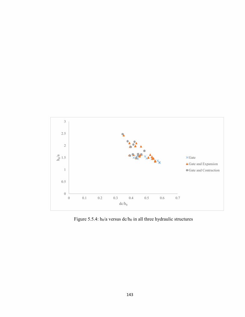
143
Figure 5.5.4: h0/a versus dc/h0 in all three hydraulic structures
0
0.5
1
1.5
2
2.5
3
0 0.1 0.2 0.3 0.4 0.5 0.6 0.7
h 0/a
dc/h0
Gate
Gate and Expansion
Gate and Contraction
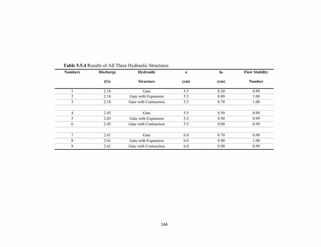
144
Table 5.5.4 Results of All Three Hydraulic Structures
Numbers Discharge
(l/s)
Hydraulic
Structure
a
(cm)
h0
(cm)
Flow Stability
Number
1 2.18 Gate 5.5 8.20 0.99 2 2.18 Gate with Expansion 5.5 8.80 1.00 3 2.18 Gate with Contraction 5.5 8.70 1.00
4 2.45 Gate 5.5 8.50 0.98 5 2.45 Gate with Expansion 5.5 8.90 0.99 6 2.45 Gate with Contraction 5.5 9.00 0.99
7 2.61 Gate 6.0 8.70 0.98 8 2.61 Gate with Expansion 6.0 8.90 1.00 9 2.61 Gate with Contraction 6.0 8.90 0.99
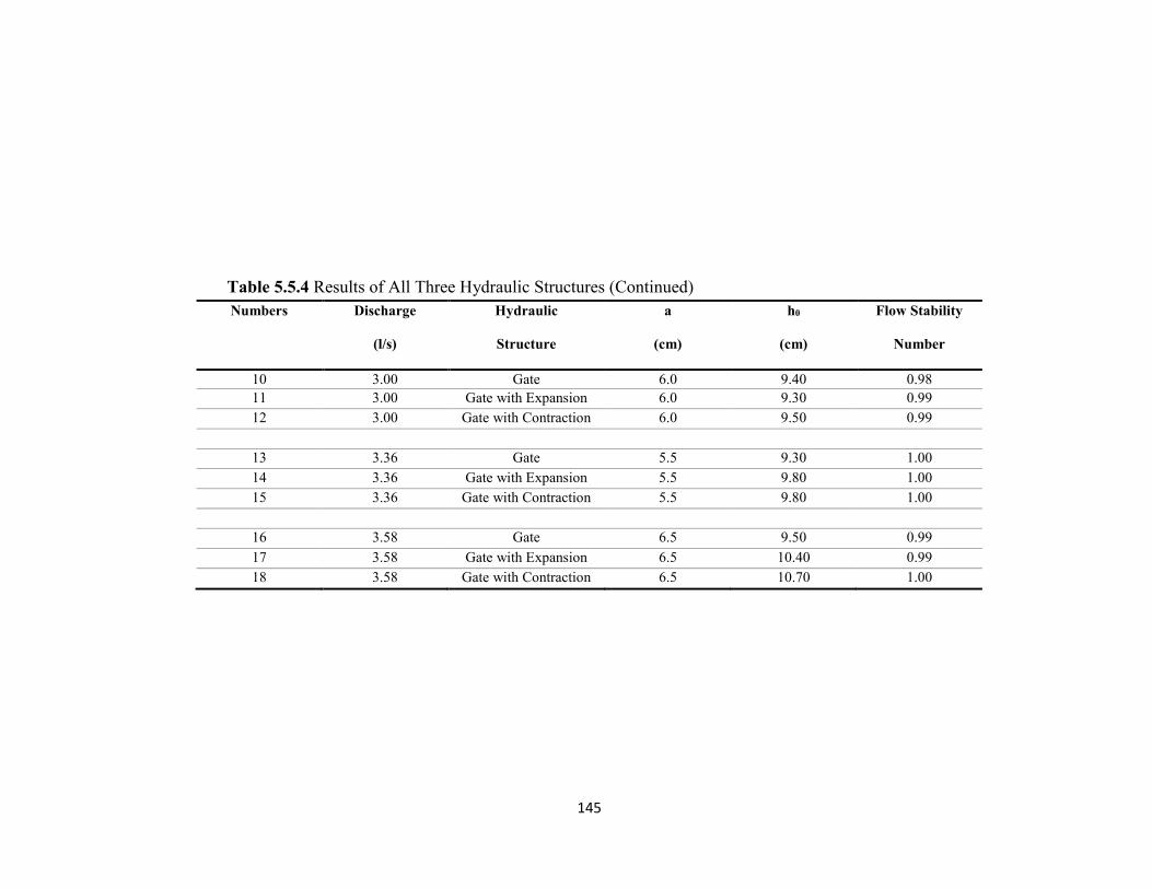
145
Table 5.5.4 Results of All Three Hydraulic Structures (Continued) Numbers Discharge
(l/s)
Hydraulic
Structure
a
(cm)
h0
(cm)
Flow Stability
Number
10 3.00 Gate 6.0 9.40 0.98 11 3.00 Gate with Expansion 6.0 9.30 0.99 12 3.00 Gate with Contraction 6.0 9.50 0.99
13 3.36 Gate 5.5 9.30 1.00 14 3.36 Gate with Expansion 5.5 9.80 1.00 15 3.36 Gate with Contraction 5.5 9.80 1.00
16 3.58 Gate 6.5 9.50 0.99 17 3.58 Gate with Expansion 6.5 10.40 0.99 18 3.58 Gate with Contraction 6.5 10.70 1.00
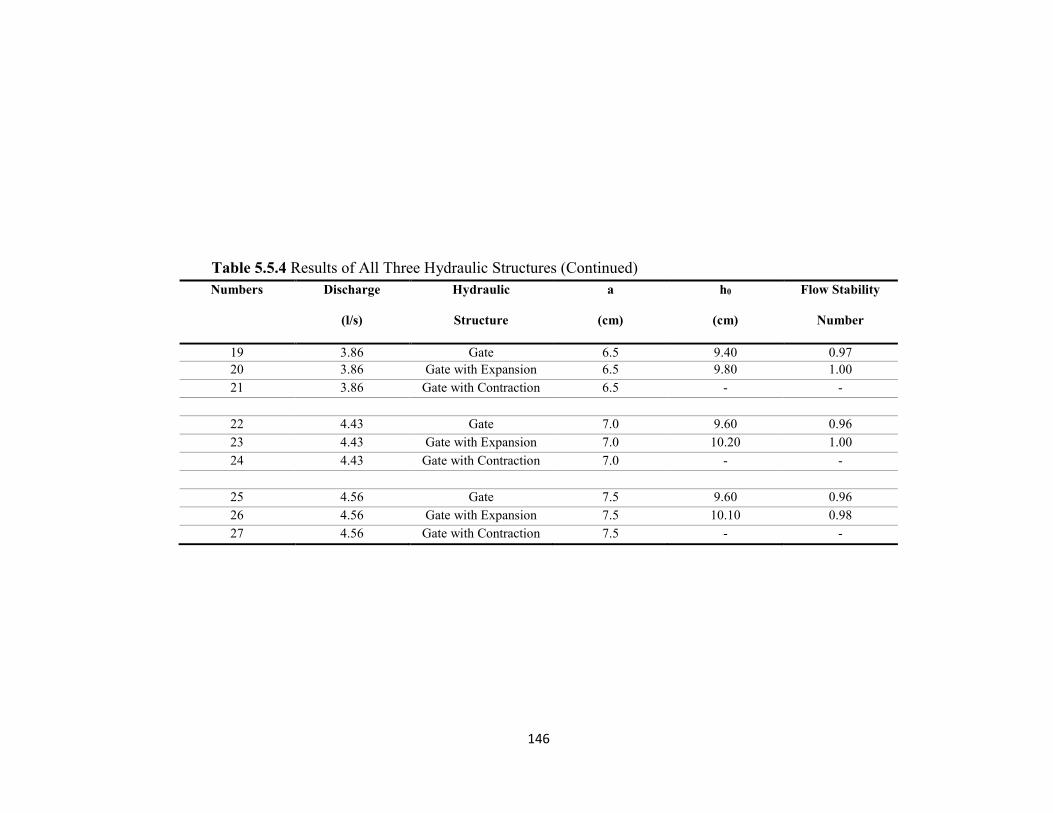
146
Table 5.5.4 Results of All Three Hydraulic Structures (Continued)
Numbers Discharge
(l/s)
Hydraulic
Structure
a
(cm)
h0
(cm)
Flow Stability
Number
19 3.86 Gate 6.5 9.40 0.97 20 3.86 Gate with Expansion 6.5 9.80 1.00 21 3.86 Gate with Contraction 6.5 - -
22 4.43 Gate 7.0 9.60 0.96 23 4.43 Gate with Expansion 7.0 10.20 1.00 24 4.43 Gate with Contraction 7.0 - -
25 4.56 Gate 7.5 9.60 0.96 26 4.56 Gate with Expansion 7.5 10.10 0.98 27 4.56 Gate with Contraction 7.5 - -
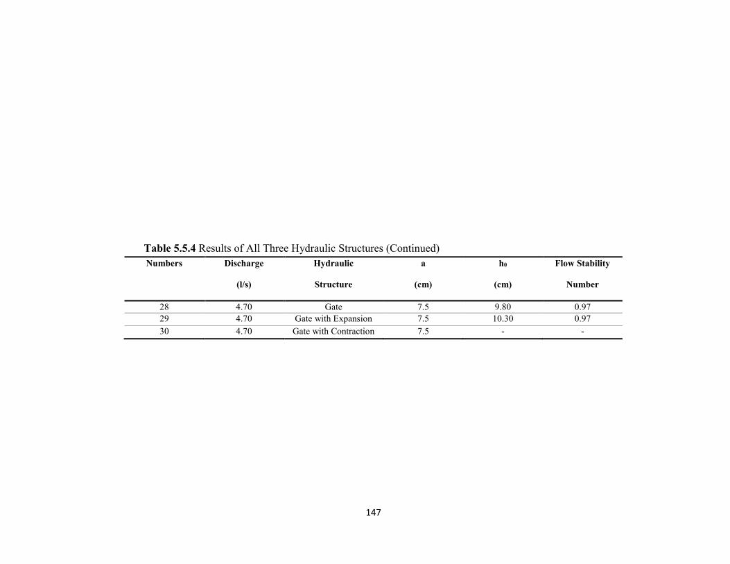
147
Table 5.5.4 Results of All Three Hydraulic Structures (Continued)
Numbers Discharge
(l/s)
Hydraulic
Structure
a
(cm)
h0
(cm)
Flow Stability
Number
28 4.70 Gate 7.5 9.80 0.97 29 4.70 Gate with Expansion 7.5 10.30 0.97 30 4.70 Gate with Contraction 7.5 - -
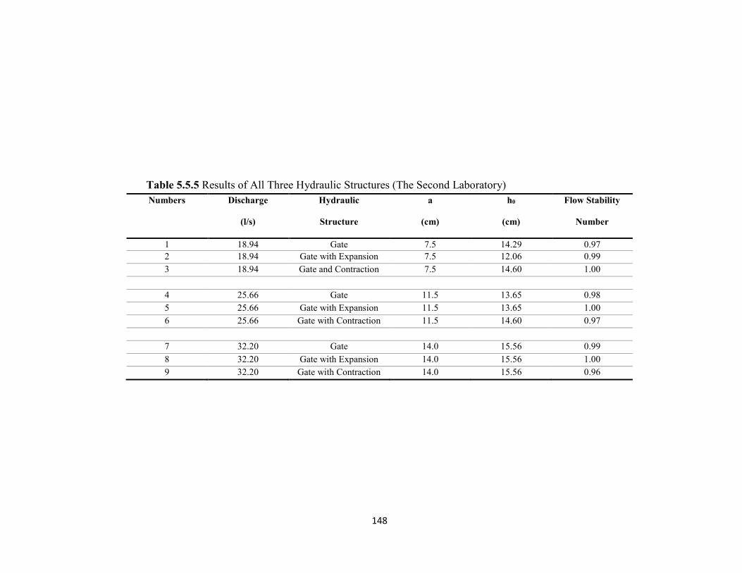
148
Table 5.5.5 Results of All Three Hydraulic Structures (The Second Laboratory) Numbers Discharge
(l/s)
Hydraulic
Structure
a
(cm)
h0
(cm)
Flow Stability
Number
1 18.94 Gate 7.5 14.29 0.97 2 18.94 Gate with Expansion 7.5 12.06 0.99 3 18.94 Gate and Contraction 7.5 14.60 1.00
4 25.66 Gate 11.5 13.65 0.98 5 25.66 Gate with Expansion 11.5 13.65 1.00 6 25.66 Gate with Contraction 11.5 14.60 0.97
7 32.20 Gate 14.0 15.56 0.99 8 32.20 Gate with Expansion 14.0 15.56 1.00 9 32.20 Gate with Contraction 14.0 15.56 0.96
149
It can be inferred from Figure 5.5.4 and Tables 5.5.4 and 5.5.5 that the performance of
a gate with expansion and a gate with contraction are better than the performance for a
gate. With additional consideration, it can be concluded that for the same gate opening
and the same discharge, a gate with contraction shows the highest upstream level and
Flow Stability Number among these three hydraulic structures across a low range of
discharges. However, the performance of a hydraulic gate with a contraction structure
is not desirable for mid- and high-range discharges. On the other hand, a gate with
expansion structures demonstrates excellent performance for low- to high-range
discharges. The results indicate that a hydraulic gate with an expansion structure
produces the highest upstream depth and Flow Stability Number across mid- and high-
range discharges among all three hydraulic structures. Moreover, the performance of a
gate with an expansion structure for low-range discharges is just slightly less than the
performance of a gate with a contraction structure. Therefore, the best hydraulic
structure which can be used across all discharge ranges to achieve the highest upstream
level, as well as the highest Flow Stability Number, is a hydraulic gate with an
expansion structure. The gate hydraulic structure can also be used across all discharge
ranges. However, its performance is less than the performance of a hydraulic gate with
an expansion structure.
5.5.4 Choose an Appropriate Hydraulic Structure
In 5.5.3, it was mentioned that among the three tested hydraulic structures two of them,
including a gate and a gate with an expansion, could be used for low to high discharge
ranges. Therefore, these two hydraulic structures are evaluated in this part to determine
150
which one is preferable in which situation. Game Theory, initially presented by Nash
[173], has been used to achieve this purpose.
Based on these results, a hydraulic gate with an expansion structure can produce a
higher upstream water level, as well as a higher Flow Stability Number than a gate
hydraulic structure under the same condition. As a result, a gate with an expansion
hydraulic structure is better able to protect the environment than a gate. On the other
hand, the construction cost of a gate hydraulic structure is lower than for a hydraulic
gate with an expansion structure.
A two-person game (a hypothetical game), with the involvement of a third-party, is
presented below to show what hydraulic structure should be selected when two
agencies try to build a hydraulic structure on the same river (at a specific distance) with
different purposes.
The assumptions in this problem are listed below:
In this problem, two agencies decide to build a hydraulic structure on the same river.
The first agency is an environmental agency and the second agency is an irrigation
agency. The irrigation agency wants to build a hydraulic structure to provide water for
agriculture, dissipate energy, and provide drinking water at a minimum cost (some of
the purposes). An environmental agency wants to build a hydraulic structure which
protects the ecosystem, avoids eutrophication, and keeps aquatic life in a normal
situation (some of the purposes). A design with strong environmental protection and a
higher cost is preferred to a design with less environmental protection and a lower cost.
Moreover, a consulting engineering company designed the hydraulic structures. The
first one is a gate hydraulic structure which is closer to the objectives of the irrigation

151
agency and the second is a hydraulic gate with an expansion structure which is closer
to the objectives of the environmental agency. Figure 3.5.5 shows the schematic of the
river and the agencies’ objectives.
Figure 5.5.5: Schematic of the river
Each agency derives some benefits from using one of these designs. In Figure 5.5.6,
the benefits for each player of the game are reported on a 0-1 scale for an economic
design, which is a gate hydraulic structure in this problem, and an environmentally-
friendly design, which is a hydraulic gate with an expansion structure in this problem.
Zero means there is no benefit for the company and one shows the maximum benefit.
The benefits are based on assumptions.
As can be seen in Figure 5.5.6, the benefit for the environmental agency for building
an environmentally-friendly design (a gate with an expansion structure) is equal to one,
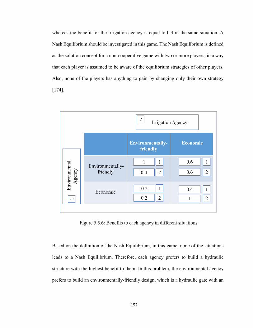
152
whereas the benefit for the irrigation agency is equal to 0.4 in the same situation. A
Nash Equilibrium should be investigated in this game. The Nash Equilibrium is defined
as the solution concept for a non-cooperative game with two or more players, in a way
that each player is assumed to be aware of the equilibrium strategies of other players.
Also, none of the players has anything to gain by changing only their own strategy
[174].
Figure 5.5.6: Benefits to each agency in different situations
Based on the definition of the Nash Equilibrium, in this game, none of the situations
leads to a Nash Equilibrium. Therefore, each agency prefers to build a hydraulic
structure with the highest benefit to them. In this problem, the environmental agency
prefers to build an environmentally-friendly design, which is a hydraulic gate with an
153
expansion structure, whereas the irrigation agency prefers to build an economic design,
which is a hydraulic gate.
There is another interesting fact in this problem which is related to the existence of a
third-party. Assume that the designer (the consulting engineering company) gains a
benefit equal to one by selling the design to an agency. If both agencies ask the same
designer (the consulting engineering company) to design a hydraulic structure for them,
then the designer gains a benefit equal to two — one from the environmental agency
and one from the irrigation agency. The designer is not a decision-maker in this game.
However, based on the results of the game, the designer is the real winner — gaining a
benefit equal to two. This is a great example that shows that the winner is not
necessarily a decision-maker in the game.
5.5.5 Scale Effect
As previously mentioned, the experiments were conducted in two laboratories with
different scales. In this part, the results of the first and second laboratory are compared
to show the scale effect on the nature of the study. The graph which indicates the h0/a
versus the dc/h0 was selected to compare the results from both laboratories. Figure 5.5.7
illustrated the results of both laboratories in gates.
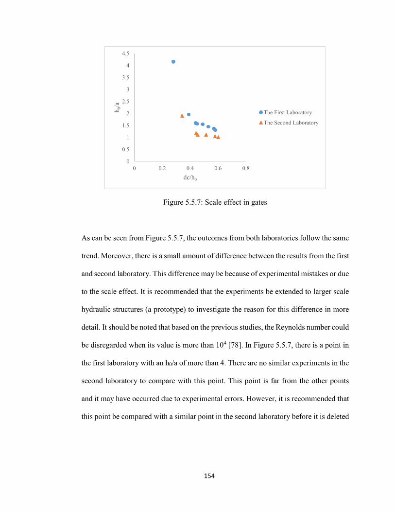
154
Figure 5.5.7: Scale effect in gates
As can be seen from Figure 5.5.7, the outcomes from both laboratories follow the same
trend. Moreover, there is a small amount of difference between the results from the first
and second laboratory. This difference may be because of experimental mistakes or due
to the scale effect. It is recommended that the experiments be extended to larger scale
hydraulic structures (a prototype) to investigate the reason for this difference in more
detail. It should be noted that based on the previous studies, the Reynolds number could
be disregarded when its value is more than 104 [78]. In Figure 5.5.7, there is a point in
the first laboratory with an h0/a of more than 4. There are no similar experiments in the
second laboratory to compare with this point. This point is far from the other points
and it may have occurred due to experimental errors. However, it is recommended that
this point be compared with a similar point in the second laboratory before it is deleted
0
0.5
1
1.5
2
2.5
3
3.5
4
4.5
0 0.2 0.4 0.6 0.8
h 0/a
dc/h0
The First Laboratory
The Second Laboratory
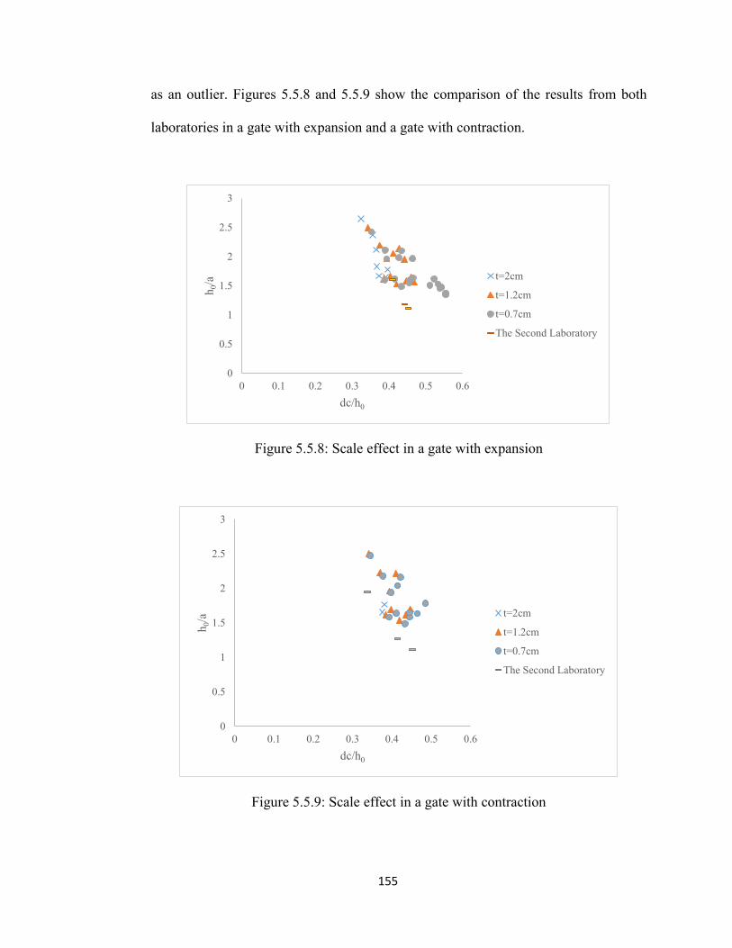
155
as an outlier. Figures 5.5.8 and 5.5.9 show the comparison of the results from both
laboratories in a gate with expansion and a gate with contraction.
Figure 5.5.8: Scale effect in a gate with expansion
Figure 5.5.9: Scale effect in a gate with contraction
0
0.5
1
1.5
2
2.5
3
0 0.1 0.2 0.3 0.4 0.5 0.6
h 0/a
dc/h0
t=2cm
t=1.2cm
t=0.7cm
The Second Laboratory
0
0.5
1
1.5
2
2.5
3
0 0.1 0.2 0.3 0.4 0.5 0.6
h 0/a
dc/h0
t=2cm
t=1.2cm
t=0.7cm
The Second Laboratory

156
The Reynolds number was recorded in a range of 8816 to 27000 in this research (the
first laboratory). Moreover, the Froude number was recorded in a range of 0.3 to 2.77
in the first laboratory. The results of the experiments indicate that the Reynolds number
is less than 104 in all stable conditions which provides a fundamental, reasonable
explanation for the scale effect observed between the various experimental set-ups.
Figures 5.5.8 and 5.5.9 show that, again, the results of both laboratories follow the same
trend, but with a small amount of difference. Some researchers [5, 114, 89] selected
one type of regression (like exponential) to develop a stage-discharge relationship in
gates and suggested using this kind of regression with different coefficients for
different scales. The coefficients should be determined separately in each structure.
Due to the lack of data in this research, it is not reasonable to develop any kind of
relationship based on the graphs. In Appendix G, some pictures of the real scale
hydraulic structures are provided for better understanding. These structures are located
in South Florida.
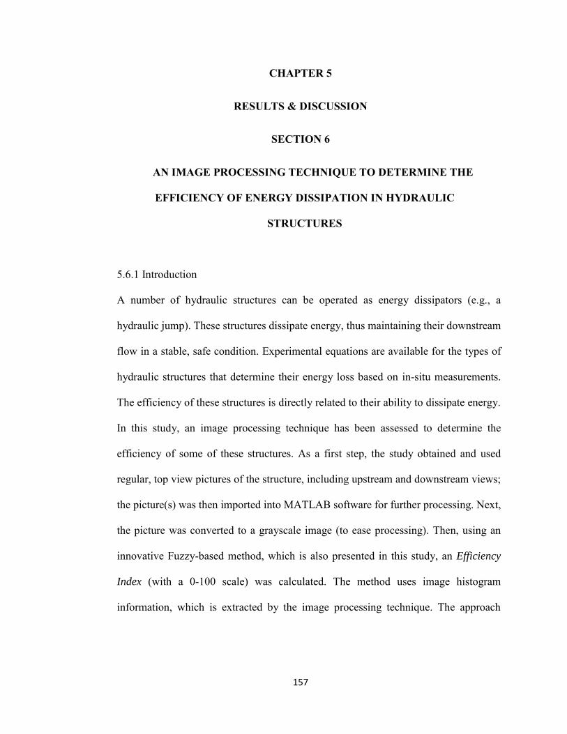
157
CHAPTER 5
RESULTS & DISCUSSION
SECTION 6
AN IMAGE PROCESSING TECHNIQUE TO DETERMINE THE
EFFICIENCY OF ENERGY DISSIPATION IN HYDRAULIC
STRUCTURES
5.6.1 Introduction
A number of hydraulic structures can be operated as energy dissipators (e.g., a
hydraulic jump). These structures dissipate energy, thus maintaining their downstream
flow in a stable, safe condition. Experimental equations are available for the types of
hydraulic structures that determine their energy loss based on in-situ measurements.
The efficiency of these structures is directly related to their ability to dissipate energy.
In this study, an image processing technique has been assessed to determine the
efficiency of some of these structures. As a first step, the study obtained and used
regular, top view pictures of the structure, including upstream and downstream views;
the picture(s) was then imported into MATLAB software for further processing. Next,
the picture was converted to a grayscale image (to ease processing). Then, using an
innovative Fuzzy-based method, which is also presented in this study, an Efficiency
Index (with a 0-100 scale) was calculated. The method uses image histogram
information, which is extracted by the image processing technique. The approach
158
herein described offers an alternative technique that hydraulic structure managers may
develop to support their operation.
5.6.2 Digital Pictures
Each picture is made from elements which are known as the pixel. There is some
information in each pixel which represents a color. Simply put, the color in each section
of the picture is represented by a pixel. The quality of the image can be determined by
the intensity of the pixels; a higher quality picture needs more pixels and greater
resolution [175].
Colored and black and white photos are two types of images. Colored pictures are made
up of three basic colors (red, green, and blue (RGB)) in three layers with 16.7 million
spectra, whereas black and white pictures are made by gray level with 256-color spectra
ranging from 0 to 255 [176]. Some other types of color images, such as CMYK (cyan,
magenta, yellow, and black), have more than three basic colors with 4.3 billion spectra.
With image processing techniques, some information can be extracted from the image.
This process is known as digitization[178].
It is easier to extract data from black and white images than from colored images,
because in colored images there is one layer for each basic color (in total, three layers)
and millions and billions of spectra. The huge amount of information in colored images
makes analyzing these pictures very difficult.Therefore, the black and white image is
preferred, because it has just 256 spectra colors. In this research, black and white
images are used to extract information. The image frequency histogram is extracted for
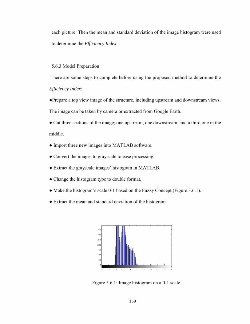
159
each picture. Then the mean and standard deviation of the image histogram were used
to determine the Efficiency Index.
5.6.3 Model Preparation
There are some steps to complete before using the proposed method to determine the
Efficiency Index:
●Prepare a top view image of the structure, including upstream and downstream views.
The image can be taken by camera or extracted from Google Earth.
● Cut three sections of the image; one upstream, one downstream, and a third one in the
middle.
● Import three new images into MATLAB software.
● Convert the images to grayscale to ease processing.
● Extract the grayscale images’ histogram in MATLAB.
● Change the histogram type to double format.
● Make the histogram’s scale 0-1 based on the Fuzzy Concept (Figure 3.6.1).
● Extract the mean and standard deviation of the histogram.
Figure 5.6.1: Image histogram on a 0-1 scale
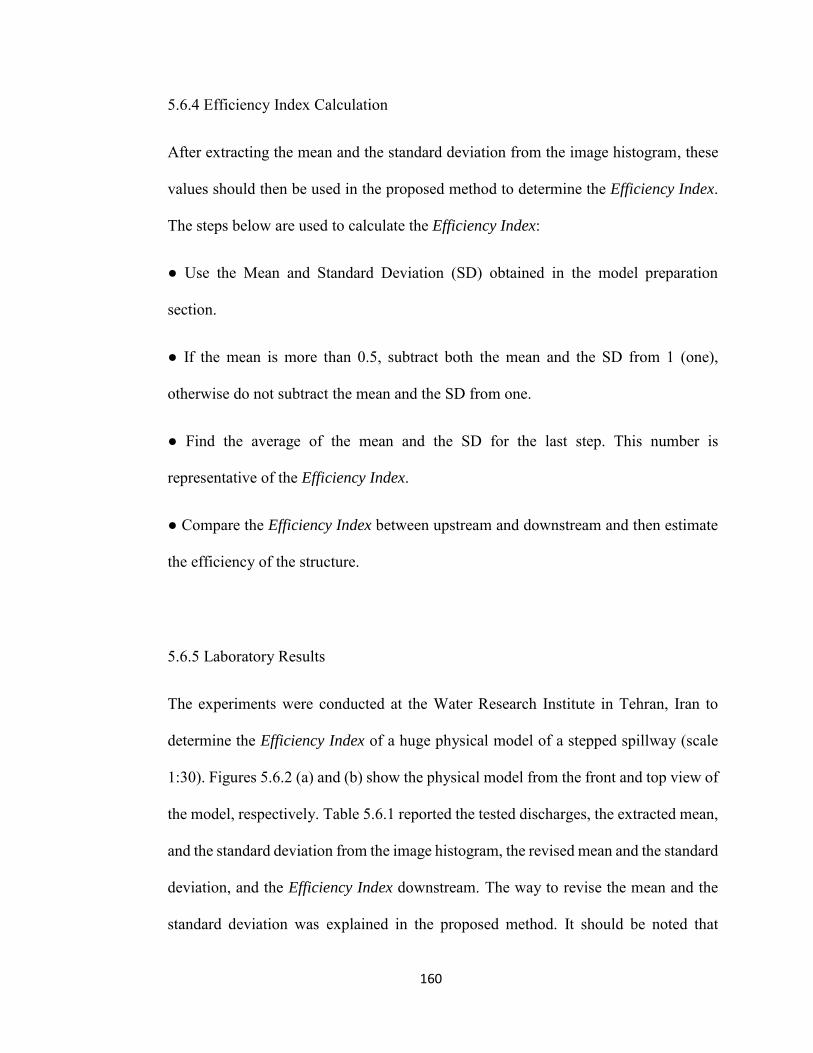
160
5.6.4 Efficiency Index Calculation
After extracting the mean and the standard deviation from the image histogram, these
values should then be used in the proposed method to determine the Efficiency Index.
The steps below are used to calculate the Efficiency Index:
● Use the Mean and Standard Deviation (SD) obtained in the model preparation
section.
● If the mean is more than 0.5, subtract both the mean and the SD from 1 (one),
otherwise do not subtract the mean and the SD from one.
● Find the average of the mean and the SD for the last step. This number is
representative of the Efficiency Index.
● Compare the Efficiency Index between upstream and downstream and then estimate
the efficiency of the structure.
5.6.5 Laboratory Results
The experiments were conducted at the Water Research Institute in Tehran, Iran to
determine the Efficiency Index of a huge physical model of a stepped spillway (scale
1:30). Figures 5.6.2 (a) and (b) show the physical model from the front and top view of
the model, respectively. Table 5.6.1 reported the tested discharges, the extracted mean,
and the standard deviation from the image histogram, the revised mean and the standard
deviation, and the Efficiency Index downstream. The way to revise the mean and the
standard deviation was explained in the proposed method. It should be noted that
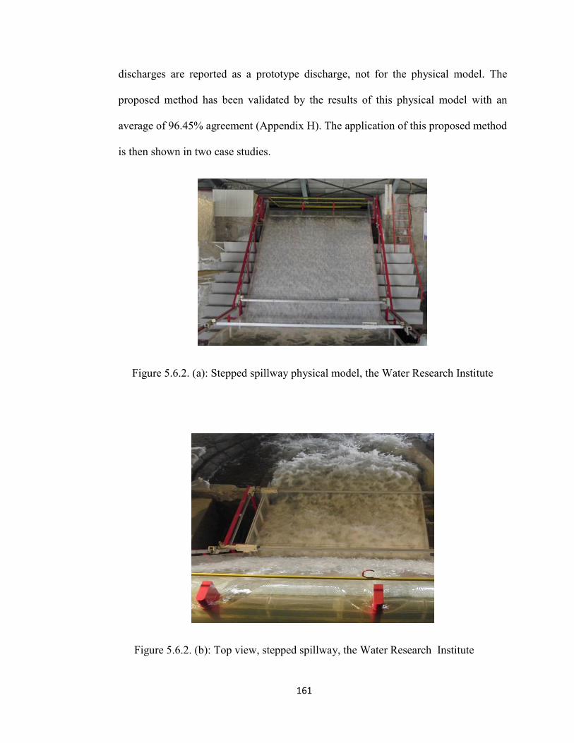
161
discharges are reported as a prototype discharge, not for the physical model. The
proposed method has been validated by the results of this physical model with an
average of 96.45% agreement (Appendix H). The application of this proposed method
is then shown in two case studies.
Figure 5.6.2. (a): Stepped spillway physical model, the Water Research Institute
Figure 5.6.2. (b): Top view, stepped spillway, the Water Research Institute
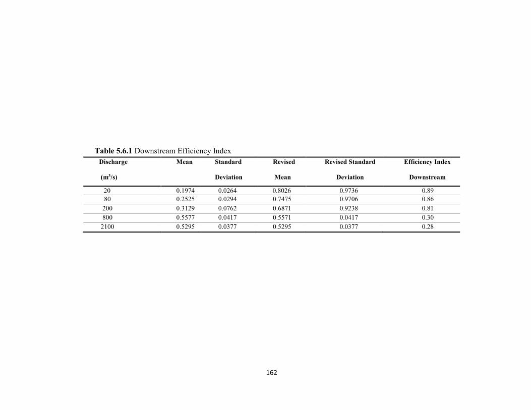
162
Table 5.6.1 Downstream Efficiency Index Discharge
(m3/s)
Mean
Standard
Deviation
Revised
Mean
Revised Standard
Deviation
Efficiency Index
Downstream
20 0.1974 0.0264 0.8026 0.9736 0.89 80 0.2525 0.0294 0.7475 0.9706 0.86 200 0.3129 0.0762 0.6871 0.9238
0.81 800 0.5577 0.0417 0.5571 0.0417 0.30 2100 0.5295 0.0377 0.5295 0.0377 0.28
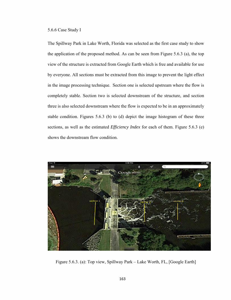
163
5.6.6 Case Study I
The Spillway Park in Lake Worth, Florida was selected as the first case study to show
the application of the proposed method. As can be seen from Figure 5.6.3 (a), the top
view of the structure is extracted from Google Earth which is free and available for use
by everyone. All sections must be extracted from this image to prevent the light effect
in the image processing technique. Section one is selected upstream where the flow is
completely stable. Section two is selected downstream of the structure, and section
three is also selected downstream where the flow is expected to be in an approximately
stable condition. Figures 5.6.3 (b) to (d) depict the image histogram of these three
sections, as well as the estimated Efficiency Index for each of them. Figure 5.6.3 (e)
shows the downstream flow condition.
Figure 5.6.3. (a): Top view, Spillway Park – Lake Worth, FL, [Google Earth]
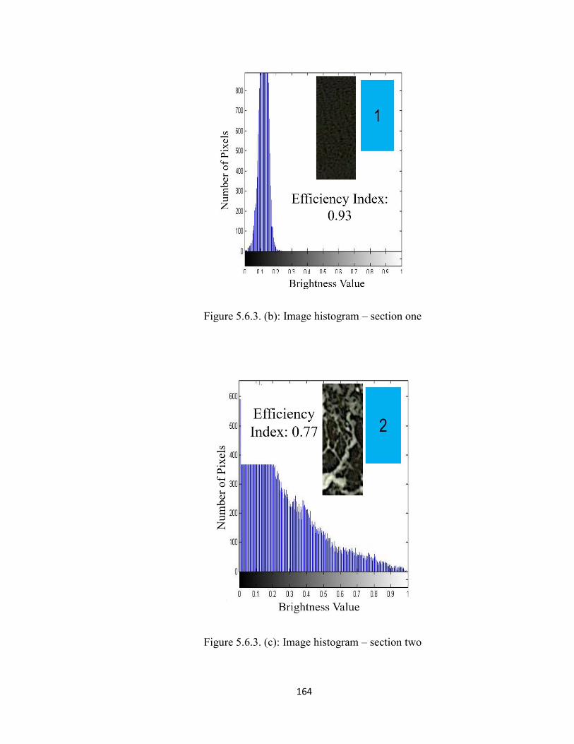
164
Figure 5.6.3. (b): Image histogram – section one
Figure 5.6.3. (c): Image histogram – section two
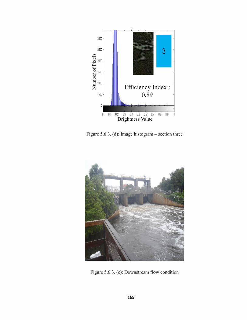
165
Figure 5.6.3. (d): Image histogram – section three
Figure 5.6.3. (e): Downstream flow condition
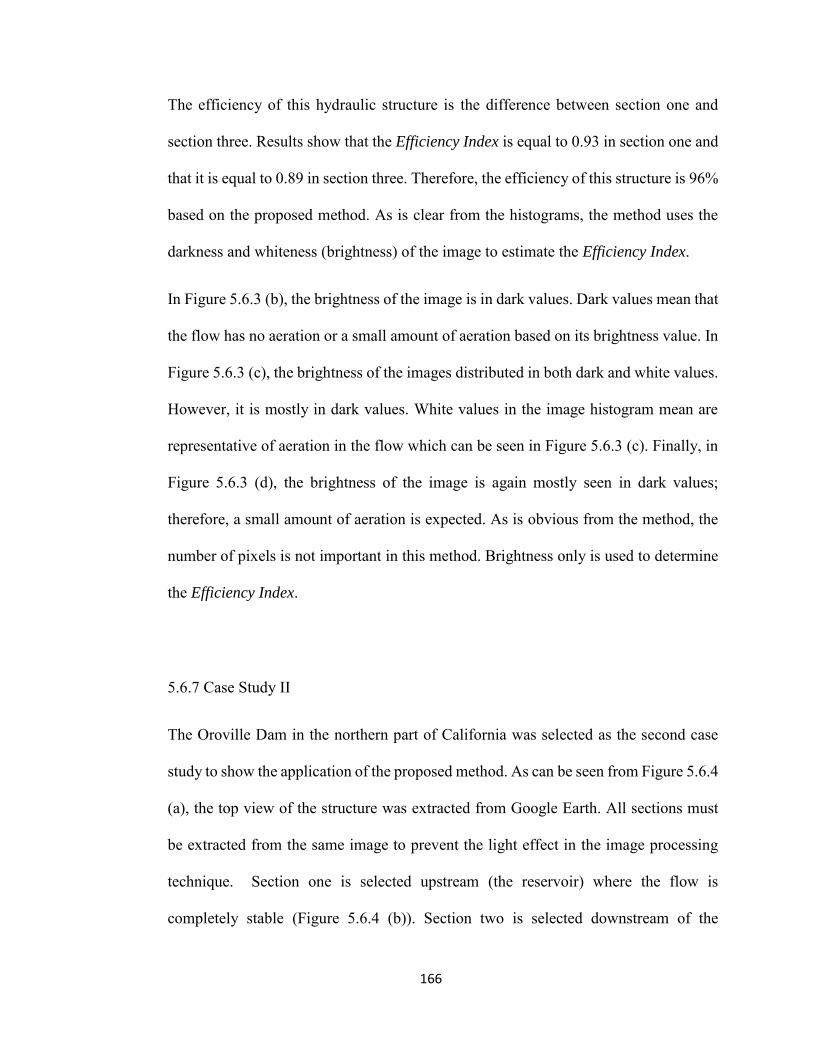
166
The efficiency of this hydraulic structure is the difference between section one and
section three. Results show that the Efficiency Index is equal to 0.93 in section one and
that it is equal to 0.89 in section three. Therefore, the efficiency of this structure is 96%
based on the proposed method. As is clear from the histograms, the method uses the
darkness and whiteness (brightness) of the image to estimate the Efficiency Index.
In Figure 5.6.3 (b), the brightness of the image is in dark values. Dark values mean that
the flow has no aeration or a small amount of aeration based on its brightness value. In
Figure 5.6.3 (c), the brightness of the images distributed in both dark and white values.
However, it is mostly in dark values. White values in the image histogram mean are
representative of aeration in the flow which can be seen in Figure 5.6.3 (c). Finally, in
Figure 5.6.3 (d), the brightness of the image is again mostly seen in dark values;
therefore, a small amount of aeration is expected. As is obvious from the method, the
number of pixels is not important in this method. Brightness only is used to determine
the Efficiency Index.
5.6.7 Case Study II
The Oroville Dam in the northern part of California was selected as the second case
study to show the application of the proposed method. As can be seen from Figure 5.6.4
(a), the top view of the structure was extracted from Google Earth. All sections must
be extracted from the same image to prevent the light effect in the image processing
technique. Section one is selected upstream (the reservoir) where the flow is
completely stable (Figure 5.6.4 (b)). Section two is selected downstream of the
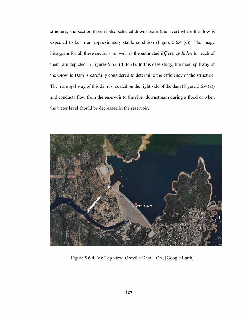
167
structure, and section three is also selected downstream (the river) where the flow is
expected to be in an approximately stable condition (Figure 5.6.4 (c)). The image
histogram for all these sections, as well as the estimated Efficiency Index for each of
them, are depicted in Figures 5.6.4 (d) to (f). In this case study, the main spillway of
the Oroville Dam is carefully considered to determine the efficiency of the structure.
The main spillway of this dam is located on the right side of the dam (Figure 5.6.4 (a))
and conducts flow from the reservoir to the river downstream during a flood or when
the water level should be decreased in the reservoir.
Figure 5.6.4. (a): Top view, Oroville Dam – CA, [Google Earth]
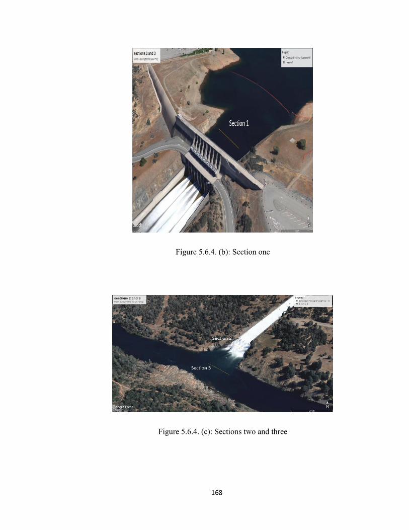
168
Figure 5.6.4. (b): Section one
Figure 5.6.4. (c): Sections two and three
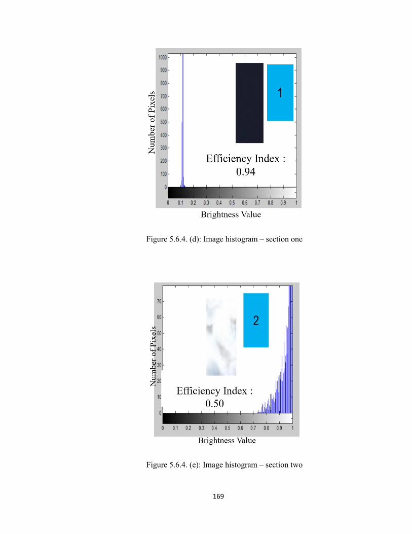
169
Figure 5.6.4. (d): Image histogram – section one
Figure 5.6.4. (e): Image histogram – section two
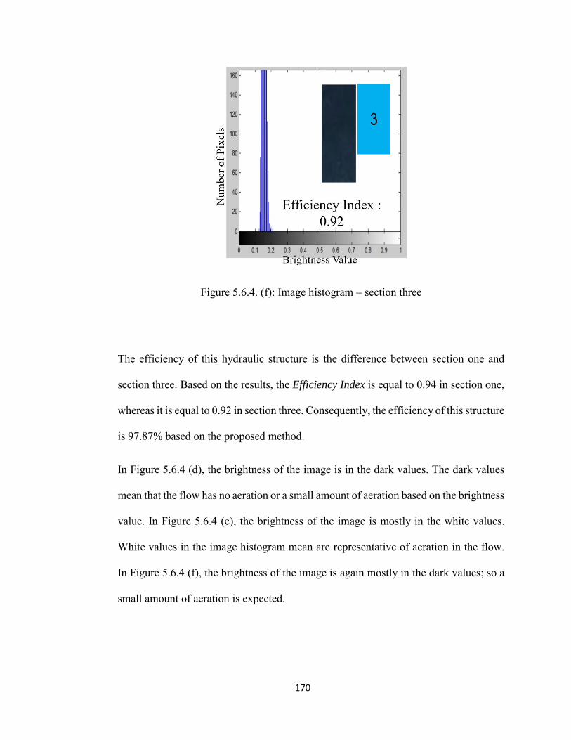
170
Figure 5.6.4. (f): Image histogram – section three
The efficiency of this hydraulic structure is the difference between section one and
section three. Based on the results, the Efficiency Index is equal to 0.94 in section one,
whereas it is equal to 0.92 in section three. Consequently, the efficiency of this structure
is 97.87% based on the proposed method.
In Figure 5.6.4 (d), the brightness of the image is in the dark values. The dark values
mean that the flow has no aeration or a small amount of aeration based on the brightness
value. In Figure 5.6.4 (e), the brightness of the image is mostly in the white values.
White values in the image histogram mean are representative of aeration in the flow.
In Figure 5.6.4 (f), the brightness of the image is again mostly in the dark values; so a
small amount of aeration is expected.
171
Section two can be used to determine the efficiency of the chute when the stilling basin
or any other type of combination is available. Moreover, the results of this section can
help engineers carefully monitor the performance of the hydraulic structure and find
out what is happening exactly in the middle of the structure or immediately after the
structure. Based on the results of this study, the following outcomes can be highlighted:
● The proposed method effectively estimated the efficiency of the hydraulic structures
in both the laboratory and the prototype.
●The proposed method, which utilizes the Image Processing Technique, is a
trustworthy, quick, low-cost, and practical method for engineers to monitor hydraulic
structures.
● The proposed method is simple because the pictures can be easily obtained from
Google Earth.
172
CHAPTER 5
RESULTS & DISCUSSION
SECTION 7
LIMITATIONS
The concepts and methods that have been introduced and developed in this research
have limitations (or constraints) that must be acknowledged. These concepts and
methods include the Flow Stability Factor, the Flow Stability Number, and the image
processing technique. Moreover, there are some additional factors, like the impact of
the Reynolds number, which limit the results. The limitations on this research are listed
in this section.
The Flow Stability Factor is a visual method and does not need any measurement,
because it is based on observation. Therefore, the individual who uses this method
should be an educated, trained expert in hydraulic engineering. This requirement is
important to ensure the correct classification of the flow into a category. This method
is based on surface flow fluctuations.
The Flow Stability Number is not defined for supercritical flow and, consequently, is
only applicable to critical and subcritical flows. This method requires measuring depth
and velocity. Thus, it is more elaborate and quantitative than the Flow Stability Factor.
An expert using this method must be familiar with the concept of permissible velocity,
the meaning and role of the energy equation, and basic statistical analysis.
173
The outcomes of this research indicate that scale has an effect on the results. The scale
effect has been assessed using the differences in the experimental results at the two
utilized laboratories and experimental flumes. The effect may be connected with the
range of the Reynolds number. Based on the literature review, results from conditions
of a Reynolds number of less than 104 cannot ensure Froude similarity, which was the
case for this research. Conclusively, additional experimentation is needed to improve
the understanding of the scale effect, and its implication in the transitioning laboratory
and pilot conditions to real prototypes.
The Efficiency Index method also has limitations. In this method, the top view picture
should capture the entire structure, fully covering the upstream and downstream areas,
in one picture. Then, three sections should be selected from the captured picture. The
method works based on the image processing technique and is able to estimate the
Efficiency Index for each selected section based on the darkness and whiteness of the
picture. If different pictures (instead of one picture) are used for different sections, the
quality of the pictures (resolution) may not be the same. Hence, the method cannot be
applied.
Because shadows have an effect on results, it is important to select areas without a
shadow, or better yet, to use a picture without a shadow. Another limitation of this
method is the availability of real time pictures. For instance, Google Earth provides
“old pictures” most of the time, which does not support the online monitoring of
structures. A person who uses this method should also be familiar with Matlab
software, image processing, hydraulic structures, flow regime categories, and statistics.
174
CHAPTER 6
CONCLUSIONS AND RECOMMENDATIONS
6.1 KEY FINDINGS AND CONCLUSIONS
The focus of the research is to classify the flow condition downstream of the hydraulic
structures by introducing the Flow Stability Factor, as well as the Flow Stability
Number. These innovative factors are presented to easily classify the flow and help to
manage the hydraulic structures to maintain downstream flow in a stable condition.
Three types of structures were used in this research, including a vertical sluice gate, a
gate and an expansion structure, and a gate and a contraction structure. Researchers
have not paid a lot of attention to flow classification and energy loss investigations, and
thus, there is an information gap.
Chapter four explained the methodology, laboratory details, and the devices which
were used in this study. The experiments were conducted in two laboratories. The first
one was the Fluid Mechanics Laboratory at Florida International University (FIU) and
the second one was the Center for Research in Water Resources (CRWR) at the
University of Texas-Austin. The Flow Stability Factor and the Flow Stability Number
(as a ratio of two energies) are introduced in this chapter.
Chapter five includes seven sections, presented as results and a discussion. Section one
shows the application of the Flow Stability Factor based on the Fuzzy Concept to
classify the flow downstream of gates. Flow classification was conducted for 14
discharges and the size of the gate opening to ensure a stable condition downstream is
175
reported using dimensionless numbers. Based on this classification method, the number
one is assigned to a completely stable flow and the number zero is assigned to a
hydraulic jump (a completely unstable flow). Other numbers between zero and one are
assigned to various hydraulic conditions between a hydraulic jump and a stable
condition, like a submerged jump, a wave, and a weak wave, etc. This research
developed dimensionless parameters, using the Pi-Buckingham method that shows the
h0/a versus dc/h0 trend, while securing a stable flow condition downstream. Two data
series were used to train and validate the gate opening neural network in vertical sluice
gates. Furthermore, a regression-based post-processing method was applied to the
outputs of the artificial neural network to reduce the difference percentage in
determining the gate opening. By considering difference percentages and average
difference percentages, it can be inferred that the regression-based post-processing
method results in less difference than ANN outcomes. The regression-based post-
processing method can be used with an average difference of roughly 3%. Therefore,
it is a reliable and accurate method even if the data set is small.
All in all, simply by measuring the depth and discharge before the gate, it is possible
to find an acceptable gate opening using ANN. Section Two shows the values of the
Flow Stability Number in vertical gates. This dimensionless number is a ratio of total
energies in two sections downstream of a gate. The results show that there is a good
agreement between the Flow Stability Number and the Flow Stability Factor.
Section three and section four represent the application of the Flow Stability Number
in a gate and an expansion, as well as in a gate and a contraction hydraulic structures.
Three thicknesses were used for these two structures. The results indicate that the
176
narrowest thickness (i.e., 0.7 centimeters) generates the best results in these hydraulic
structures. Moreover, the outcomes show that there is not a meaningful difference in
the hydraulic performance between 0.7 centimeters and 1.2 centimeter thicknesses in a
gate and an expansion hydraulic structure. The greatest thickness (2 centimeters) can
be used in low rate discharges; the 1.2 cm thickness can be used in low- and mid-rate
discharges; and finally, the narrowest thickness (0.7 centimeters) can be used for all
discharge rates to produce a stable condition downstream of a gate and an expansion
hydraulic structure.
In section five, the results of the Flow Stability Number and the Flow Stability Factor
were compared. These two values demonstrate good agreement in determining the
stable condition downstream of hydraulic structures. As a result, the Flow Stability
Factor can be implemented in projects by hydraulic experts as a practical, quick, and
reliable method to determine the stability condition. There is no need to measure any
variables to determine the Flow Stability Factor; therefore, it is desirable for
applications in practical work when measurements cannot be taken. Later in section
five, three hydraulic structures were compared and the results indicate that a gate with
an expansion structure has the best hydraulic performance among these structures
across all discharge rates. Furthermore, a gate and an expansion with the smallest
thickness can be used across a wide range of discharges, whereas a gate with a
contraction hydraulic structure can only be used for low discharge rates. The flow
immediately after a gate a contraction is somehow wavy, and this hydraulic structure
is not recommended as a structure for producing a stable condition downstream.
177
Game Theory was used to select an appropriate hydraulic structure based on the
objectives of different agencies. A gate with an expansion structure is presented as a
desirable hydraulic structure for environmental agencies, because it provides the
highest degree of downstream stability for the structure. However, the construction cost
of this structure is more than the cost for a gate hydraulic structure. On the other hand,
the gate structure is presented as a desirable option for irrigation agencies, because the
construction cost is lower than for a gate with an expansion structure. Based on the
results, a Nash Equilibrium cannot be achieved in this game; therefore, each agency
should build their own most desired option. Moreover, the designer is presented as a
third-party who is not a decision-maker in the game, but who can benefit from it. If
both agencies select the same designer for their project, then, the designer is the real
winner of the game. In addition, the graphs which show the results for both laboratories,
in section five, illustrate that the flow in these structures is sensitive to a scale effect
and more consideration should be taken about sluice gate studies.
An image processing technique has been assessed to determine the efficiency of some
of the hydraulic structures in chapter five – section six. In this method, a grayscale
image should be used for processing ease. MATLAB software was used to produce a
grayscale image from a colored image (the top view of the structure) and to extract an
image histogram. Then, an innovative Fuzzy-based method should be applied to
calculate the Efficiency Index, across a 0-100 scale. The method uses image histogram
information, which is extracted by the image processing technique, and determines the
Efficiency Index based on the darkness and whiteness (brightness) of the picture in
question. One laboratory physical model and two case studies were selected to show
178
the application of the method. The method was validated with the results of the physical
method with an average 96.45% agreement. The efficiency of the structure was
calculated at 96% in the Spillway Park, Lake Worth, Florida, and as 97.87% in the
main spillway of the Oroville Dam, California. The outcomes show that this proposed
method can be effectively used to determine the efficiency of hydraulic structures in
both laboratory and real world situations. Moreover, this method can help engineers —
offering a practical, low-cost, trustworthy, and quick way to monitor hydraulic
structures. Simplicity is another advantage of this method, because the top view
pictures can be obtained from Google Earth for free and quickly.
Limitations on the methods which have been used in this research are listed in chapter
five - section seven. There are some limitations to using the Flow Stability Factor, the
Flow Stability Number, and the image processing technique. The Flow Stability Factor
is a visual method and there is no need to measure any variable in this method.
Therefore, the person who is using this method should be a hydraulic expert. The flow
is classified in some categories, and there is the chance to select the flow in an incorrect
category when the person using this method is not a hydraulic expert. The Flow
Stability Number is not defined for supercritical flow and is only applicable in critical
and subcritical flows. Also, to use this method, depths and velocities must be measured
which makes it more expensive than the Flow Stability Factor. The proposed method
to estimate the Efficiency Index and the overall efficiency of the structures also has
some limitations. In this method, one picture should be captured for the whole structure,
including both upstream and downstream. Then, three sections should be selected from
the captured picture. When different pictures are used for different sections, the quality
179
of the pictures (resolution) are not the same. Hence, the method cannot be applied.
Moreover, a shadow affects the results of the method. Therefore, when selecting the
sections, the user should try to select an area without shadows or use a picture without
shadows. Another limitation of this method is the lack of access to real time pictures.
Most of the time, Google Earth offers only old pictures, whereas for the online
monitoring of structures the most updated pictures are needed.
4.2 RECOMMENDATIONS FOR FUTURE WORK
Because of the scale effect, it is recommended that experiments be conducted in large-
scale structures (in sections one to four) to better understand a scale effect and to find
more reliable results and develop an equation which can be used to estimate the size of
the gate opening. Also, it is recommended that expansion and contraction be used with
different lenghths to find the effect of this factor on the hydraulic performance of these
structures.
Other types of structures, like stepped spillways, ogee spillways, and flip buckets, can
be combined with a gate, and then the Flow Stability Number can be estimated for
different discharges and gate openings. Therefore, the secenarios which lead to
downstream stable conditions can be determined.
The Efficiency Index is defined in chapter three – section six. However, the acceptable
range of this index should be investigated by conducting some experiments. It is
recommended that the acceptable range be found by measuring the energy and flow
aeration in different hydraulic structures.
180
BIBLIOGRAPHY
[1] Roth, A., & Hager, W. H. (1999). Underflow of standard sluice gate. Experiments in
fluids, 27(4), 339-350. [2] Wu, S., & Rajaratnam, N. (2015). Solutions to rectangular sluice gate flow problems. Journal of Irrigation and Drainage Engineering, 141(12), 06015003. [3] Akoz, M. S., Kirkgoz, M. S., & Oner, A. A. (2009). Experimental and numerical modeling of a sluice gate flow. Journal of Hydraulic Research, 47(2), 167-176. [4] Altan-Sakarya, A. B., & Kökpınar, M. A. (2013). Computation of discharge for simultaneous flow over weirs and below gates (H-weirs). Flow Measurement and
Instrumentation, 29, 32-38. [5] Bijankhan, M., Ferro, V., & Kouchakzadeh, S. (2012). New stage-discharge relationships for radial gates. Journal of Irrigation and Drainage Engineering, 139(5), 378-387. [6] Henderson, F. M. (1966). Open channel flow, Macmillan, New York.
[7] Shammaa, Y., Zhu, D. Z., & Rajaratnam, N. (2005). Flow upstream of orifices and sluice gates. Journal of Hydraulic Engineering, 131(2), 127-133. [8] Subramanya, K. (1982). Flow in open channels, National Book Trust, India.
[9] Kim, Y., Choi, G., Park, H., & Byeon, S. (2015). Hydraulic Jump and Energy Dissipation with Sluice Gate. Water, 7(9), 5115-5133. [10] Swamee, P. K. (1992). Sluice-gate discharge equations. Journal of Irrigation and
Drainage Engineering, 118(1), 56-60. [11] Cassan, L., & Belaud, G. (2011). Experimental and numerical investigation of flow under sluice gates. Journal of Hydraulic Engineering, 138(4), 367-373. [12] Shahrokhnia, M. A., & Javan, M. (2006). Dimensionless stage–discharge relationship in radial gates. Journal of irrigation and drainage engineering, 132(2), 180-184. [13] Yen, J. F., Lin, C. H., & Tsai, C. T. (2001). Hydraulic characteristics and discharge control of sluice gates. Journal of the Chinese Institute of Engineers, 24(3), 301-310. [14] Hamedi, A., & Fuentes, H. R. (2016). New Relationship between a Vertical Gate Opening and Downstream Flow Stability: Experimental Development. In World
Environmental and Water Resources Congress 2016 (pp. 47-57).
181
[15] Boileau P. (1848). MeHmoire sur le jaugeage des cours d'eau a` faible ou a` moyenne section. Journal Ecole Polytechnique Paris 33. [16] Bornemann KR. (1871). Versuche uK ber den Aus¯uss unter Wasser bei SchuK tzen. Civilingenieur 17: 45-60. [17] Bornemann KR. (1880). UG ber den Aus¯uss bei SchuK tzen und schuK tzenartigen MuK ndungen. Civilingenieur 26: 297-376. [18] Haberstroh CE. (1890). Experiments on flow of water through large gates and over wide crests. Journal of Association Engineering Society 5: 1-11. [19] von Mises, R. (1917). Berechnung von ausfluß und ueberfallzahlen, Zeitschrift des Vereine Deutscher Ingenieure, Berlin (in German). [20] Gibson, A. (1919). Experiments on the coefficients on discharge under rectangular sluice gates. (Abridges). In Minutes of the Proceedings of the Institution of Civil
Engineers (Vol. 207, No. 1919, pp. 427-434). Thomas Telford-ICE Virtual Library. [21] Hurst HE; Watt DAF. (1925). The similarity of motion of water through sluices of the Assuan dam. Proceeding of Institution of Civil Engineering. 218: 72-180. [22] Keutner, C. (1932). WasserabfuK hrungsvermoKgen von scharfkantigen und abgerundeten PlanschuK tzen. Bautechnik 10: 266-269; 10:303-305. [23] Keutner, C. (1935). Die StroKmungsvorgaKnge an unterstroKmten SchuK tztafeln mit scharfen und abgerundeten Unterkanten. Wasserkraft und Wasserwirtschaft 30: 5-8; 30: 16-21. [24] Woycicki, K. (1935). The hydraulic jump on its role on discharge of sluice gates. Technical Rep. No. 3-2, U.S. Bureau of Reclamation, Denver, 65. [25] Fawer, C. (1937). Calcul de la contraction causeHe par une vanne plane dans le cas d'un eHcoulement deHnoyeH. Bulletin Technique de la Suisse Romande 63: 192-198; 63: 217-219; 63: 245-252; 63: 283-287. [26] Escande, L. (1938). Etude theHorique et expeHrimentale de l'eHcoulement par vanne de fond. Revue GeHneHrale de l'Hydraulique 4: 25-29; 4:120-128. [27] Gentilini, B. (1941). Ef¯usso dalle luci soggiacenti alle paratoie piane inclinate e a settore. L'Energia Elettrica 18: 361-380. [28] Metzler, D. E. (1948). A model study of Tainter gate operation. MS thesis, Iowa State
Univ., Iowa City, Iowa.
182
[29] Smetana, J. (1948). Ecoulement de l'eau au-dessous d'une vanne et forme rationelle de la surface d'appui de la vanne. La Houille Blanche 4: 126-146. [30] Henry, H. R. (1950). Discussion of ‘Diffusion of Submerged Jets. Trans. ASCE, 115, 687–694. [31] Binnie, A. M. (1952). The flow of water under a sluice-gate. Quarterly Journal of
Mechanics and Applied Mathematics, Oxford, England, 4,395-407. [32] Marchi, E. (1953). Sui fenomeni di efflusso piano da luci a battente. Ann. Mat. Pura
Appl., 35(1), 327–341 (in Italian). [33] Benjamin, T. B. (1955). On the flow in channels when rigid obstacles are placed in the stream. Journal of Fluid Mechanics, 1, 227–248. [34] Franke, P. G. (1956). Theoretische Betrachtungen zur Strahlkontraktion beim Ausfluss unter Schu¨tzen. Bautechnik, 33(3), 73–77 (in German). [35] Toch, A. (1955). Discharge characteristics of Tainter gates. Trans. American Society
of Civil Engineers, 120, 290–300. [36] Chow, V.T. (1959). Open channel hydraulics. McGraw-Hill Book Company, Inc; New
York.
[37] King, H.W., (1963). Handbook of Hydraulics, 5th Edition, McGraw-Hill, New York.
[38] Anwar, H. O. (1964). Discharge coefficients for control gates. WaterPower, 17(4), 152–159. [39] Rajaratnam, N., and Subramanya, K. (1967). Flow equation for the sluice gate. Journal Irrigation and Drainage Engineering, 93(3), 167–186. [40] Rajaratnam, N., & Subramanya, K. (1967). Flow immediately below submerged sluice gate. Journal of the Hydraulics Division, 93(4), 57-77. [41] Allen, J., and Hamid, H. I. (1968). The hydraulic jump and other phenomena associated with flow under rectangular sluice-gates. Proceeding of Institution Civil
Engineering, 40, 345–362. [42] Fangmeier, D., and Strelkoff, T. S. (1968). Solution for gravity flow under sluice gates. Journal of Engineering Mechanical Division, ASCE, 94(1), 153-176. [43] Barr, D. I. H., Huq, S. S., and Skaikh, A. H. (1969). Discussion of ‘The hydraulic jump and other phenomena associated with flow under rectangular sluice-gates,’ by J. Allen and H. I. Hamid. Proceeding o, Institution of Civil Engineering, 42, 529–533.
183
[44] Larock, B. E. (1969). Gravity affected flows from planar sluice gates. Journal of
Hydraulic Division, ASCE, 95(4), 851-864. [45] Verma, D. V. S., & Goel, A. (2003). Development of efficient stilling basins for pipe outlets. Journal of irrigation and drainage engineering, 129(3), 194-200. [46] Chatterjee, S. S., Ghosh, S. N., & Chatterjee, M. (1994). Local scour due to submerged horizontal jet. Journal of Hydraulic Engineering, 120(8), 973-992. [47] Ojha, C. S. P., & Subbaiah, D. (1997). Analysis of flow through lateral slot. Journal
of irrigation and drainage engineering, 123(5), 402-405. [48] Panda, S. (1981). Characteristics of side sluice flow. ME thesis, Univ. of Roorkee,
Roorkee, India. [49] Swamee, P. K., Pathak, S. K., & Ali, M. S. (1993). Analysis of rectangular side sluice gate. Journal of irrigation and drainage engineering, 119(6), 1026-1035. [50] Ghodsian, M. (2003). Flow through side sluice gate. Journal of irrigation and
drainage engineering, 129(6), 458-463. [51] Bijankhan, M., Darvishi, E., and Kouchakzadeh, S. (2012). Discussion of ‘Energy and momentum velocity coefficients for calibrating submerged sluice gates in irrigation canals” by Oscar Castro-Orgaz, David Lozano, and Luciano Mateos. Journal of irrigation and
drainage engineering, 138(9), 852–854. [52] Bijankhan, M., and Kouchakzadeh, S. (2011). Discussion of ‘Benchmark of discharge calibration methods for submerged sluice gates’ by Carlos Sepúlveda, Manuel Gómez, and José Rodellar. Journal of irrigation and drainage engineering, 137(1), 56–57. [53] Bijankhan, M., Kouchakzadeh, S., & Bayat, E. (2011). Distinguishing condition curve for radial gates. Flow Measurement and Instrumentation, 22(6), 500-506. [54] Safarinezhad, D. (1991). Discharge algorithms for canal radial gates. MS thesis, Shiraz
Univ., Shiraz, Iran.
[55] Lin, C. H., Yen, J. F., & Tsai, C. T. (2002). Influence of sluice gate contraction coefficient on distinguishing condition. Journal of Irrigation and Drainage
Engineering, 128(4), 249-252. [56] Eei, J., (1975). Open Channel Hydraulics, Vol. 2, (in Chinese) Tung Hwa Publishing
Co., Taiwan, R.O.C.
184
[57] Cho, J. N., Kim, D. H., & Lee, S. O. (2016). Experimental Study of Shape and Pressure Characteristics of Solitary Wave generated by Sluice Gate for Various Conditions. Journal
of the Korean Society of Safety, 31(2), 70-75. [58] Kim, D. (2007). Numerical analysis of free flow past a sluice gate. KSCE Journal of Civil Engineering, 11(2), 127–132. [59] Ohtsu, I., & Yasuda, Y. (1994). Characteristics of supercritical flow below sluice gate. Journal of Hydraulic Engineering, 120(3), 332-346. [60] Nago, H. (1978). Influence of gate-shapes on discharge coefficients. Trans. Japanese
Society of Civil Engineering, 10, 116–119. [61] Alhamid, A. A. (1999). Analysis and formulation of flow through combined V-notch-gate-device. Journal of Hydraulic Research, 37(5), 697-705. [62] Negm, A. M., Alhamid, A. A., & El-Saiad, A. A. (1998). Submerged flow below sluice gate with sill. Advances in Hydroscience and Engineering, 3. [63] Abdelaal, G.M.M., (1990). Study of the free flow conditions for silled gates Unpublished M.Sc. Thesis, Faculty of Engineering, Ain Shams University, Cairo, Egypt.
[64] Negm, A.M.; Abouelatta, N. and Abdellateef, M., (1993). Supercritical free flow characteristics under silled sluice gate. Scientific Bulletin, Faculty of Engineering, Ain
Shams University, 28:4, Cairo, Egypt, pp.163-174. [65] Negm, A.M., Abdelaal, G. M., Owais, T. M., Abdellateef, M. and Hammad, M.N., (1995) Characteristics of free hydraulic jump downstream silled sluice gates. Journal of
Water and Energy International, 52:3, CBIP, India, pp.45-51. [66] Negm, A.M., (1994). Optimum relative height of the optimal under-gate sill for supercritical submerged flow below sluice Gates. 19th Int. Conf. for Statistic, Computer
Science, Scientific and Social Applications, 9-14 April, Engineering Science, Cairo, Egypt, Vol.1, pp. 39-49. [67] Negm, A. M. and El-Saiad, A. A., (1993). Subcritical submerged flow characteristics beneath silled sluice gates. Proc. of AEIC-93, December 18-21, Faculty of Engineering,
Al-Azhar University, Naser City, Cairo, Egypt, vol.4, pp. 298-309.
[68] El-Saiad, A., (1990). Study of submerged flow characteristics under silled sluice gates. Unpublished M.Sc. Thesis Ain Shams University, Cairo, Egypt.
185
[69] El-Saiad, Atef A.; Abdel Hafiz, Essam; Owais, Talaat M. and Hammad, M. N., (1991). Characteristics of submerged flow under sluice gate with sill. Ain Shams University
Engineering Bulletin, Vol.26, No.1, March, Cairo, Egypt, pp.109-120. [70] El-Saiad, Atef A.; Abdel Hafiz, Essam and Hammad, M. N., (1991). Effect of sill under gate on the discharge coefficient. Journal of the Egyptian Society of Engineers, Vol.30, No.2, pp. 13-16. [71] Abdel-Salam, M. W.; Owais, T. M., Armanious S. D. and Salem, M. N., (1990). Theoretical and experimental studies of radial gates with and without sill. Engineering
Bulletin, Faculty of Engineering, Ain Shams University, Vol.25, No.3, Cairo, Egypt, Dec., pp. 18-35. [72] Negm, A. M.; Abdellateef, M. and Owais, T. M., (1993). Effect of under-gate sill crest shapes on the flow characteristics. Proc. of AEIC-93, 18-21 Dec., Faculty of Eng., Al-Azhar
University, Naser City, Cairo, Egypt, Vol.4, pp. 230-241. [73] Salama, M., (1987). Flow below sluice gate with sill. Journal of Egyptian Society of
Engineers, Vol 26, No.4, pp. 31-36. [74] Negm AM, Al-Brahim AM, AlHamid AA. (2002). Combined free flow over weirs and below gates. Journal of Hydraulic Research ;40(3):359–65. [75] Bove, I., Acosta, D., Gutiérreza, N., Gutiérreza, V., & Sarasúa, L. G. (2013). Double scouring by turbulent jets downstream of a submerged sluice gate. arXiv preprint
arXiv:1311.4194. [76] Isaacs, L. T., and Allen, P. H. (1994). Contraction coefficients for radial sluice gates. Proc., 1994 Int. Conf. on Hydr. in Civ. Eng., Nat. Conf. Publ. No. 94/1, Institution of
Engineers, Barton, ACT, Australia, 262–265. [77] Isaacs, L.T., (1977). Numerical Solution for Flow under Sluice Gates. Journal of
Hydraulic Division, ASCE, Vol. 103, No. 5, pp. 473-481. [78] Montes, J. S. (1997). Irrotational flow and real fluid effects under planar sluice gates. Journal of Hydraulic Engineering, 123(3), 219-232. [79] Webby, M.G., (1999). Discussion of ‘Irrotational Flow and Real Fluid Effects under Planar Sluice Gates,’ Discussion by J. S. Montes, Journal of Hydraulic Division, ASCE, Vol. 125, No. 2, pp. 210-212. [80] Vanden-Broeck, J. M. (1997). Numerical calculations of the free-surface flow under a sluice gate. Journal of Fluid Mechanics, 330, 339-347.
186
[81] Bhowmik, N. G. (1971). Hydraulic Jump Type Stilling Basins for Froude Number 2.5
to 4.5. Illinois State Water Survey. [82] French, R. H. (1985). Open-channel hydraulics.
[83] Chung, Y. C. (1972). Solution of flow under sluice gates. Journal of Engineering
Mechanical Divivision, ASCE, 98(1), 121-140. [84] Buyalski, C. P. (1983). Discharge algorithms for canal radial gates. REC-ERC-83-9,
Engineering and Research Center, U.S. Bureau of Reclamation, Denver,
⟨http://www.usbr.gov/pmts/hydraulics_lab/pubs/REC/REC-ERC-83-09.pdf⟩. [85] Asavanant, J. & Vanden-Broeck, J.-M. (1996). Nonlinear free surface flows emerging from a vessel and flows under a sluice gate. Journal of Australia Mathematic Society. B 38, 63-86. [86] Vanden-Broeck, J.-M. (1986). Flow under a gate. Physics of Fluids. 29, 3148-3151.
[87] Hill, D. F., & Younkin, B. D. (2009). A simple estimation of the growth rate and equilibrium size of bedforms created by a turbulent wall jet. Journal of Hydraulic
Research, 47(5), 619-625. [88] Wahl, T. (2005). Refined energy correction for calibration of submerged radial gates. Journal of Hydraulic Engineering, 131(6), 457–466. [89] Ansar M. (2001). Discussion of Simultaneous flow over and under a gate by V Ferro. Journal of Irrigation and Drainage Engineering, ASCE; 127(5):325–6. [90] Clemmens, A. J., Strelkoff, T. S., and Replogle, J. A. (2003). Calibration of submerged radial gates. Journal of Hydraulic Engineering, 129(9), 680–687. [91] U.S. Bureau of Reclamation (USBR). (2001). Water measurement manual, 3rd Ed.,
U.S. Dept. of the Interior, Washington, DC
[92] Wahl, T. L., and Clemmens, A. J. (2005). Applying the energy-momentum method to radial gate discharge calibration. Impacts of Global Climate Change, ASCE, Reston, VA. [93] Alminagorta, O., and Merkley, G. P. (2009). Transitional flow between orifice and nonorifice regimes at a rectangular sluice gate. Journal of Irrigation and Drainage
Engineering, 135(3), 382–387. [94] Smith, C. D. (1977). Discussion of ‘Free flow immediately below sluice gates,’ by Nallamuthu Rajaratnam. Jounal of Hydraulic Division, ASCE, 123(11), 1371–1373.
187
[95] Rajaratnam, N., & Macdougall, R. K. (1983). Erosion by plane wall jets with minimum tailwater. Journal of Hydraulic Engineering, 109(7), 1061-1064. [96] Rajaratnam, N. (1981). Erosion by plane turbulent jets. Journal of hydraulic Research, 19(4), 339-358. [97] Balachandar, R., & Kells, J. A. (1997). Local channel in scour in uniformly graded sediments: the time-scale problem. Canadian journal of civil engineering, 24(5), 799-807. [98] Balachandar, R., & Kells, J. A. (1998). Instantaneous water surface and bed scour profiles using video image analysis. Canadian Journal of Civil Engineering, 25(4), 662-667. [99] Rajaratnam, N. (1977). Free flow immediately below sluice gates. Journal of the
Hydraulics Division, 103(4), 345-351. [100] Masliyah, J. H., Nandakumar, K., Hemphill, F., & Fung, L. (1985). Body-fitted coordinates for flow under sluice gates. Journal of Hydraulic Engineering, 111(6), 922-933. [101] Rajaratnam, N., & Humphries, J. A. (1982). Free flow upstream of vertical sluice gates. Journal of Hydraulic Research, 20(5), 427-437. [102] Kells, J. A., Balachandar, R., & Hagel, K. P. (2001). Effect of grain size on local channel scour below a sluice gate. Canadian Journal of Civil Engineering, 28(3), 440-451. [103] Habibzadeh, A., Vatankhah, A. R., & Rajaratnam, N. (2011). Role of energy loss on discharge characteristics of sluice gates. Journal of Hydraulic engineering, 137(9), 1079-1084. [104] Balachandar, R., Kells, J. A., & Thiessen, R. J. (2000). The effect of tailwater depth on the dynamics of local scour. Canadian Journal of Civil Engineering, 27(1), 138-150. [105] Bey, A., Faruque, M. A., & Balachandar, R. (2007). Two-dimensional scour hole problem: role of fluid structures. Journal of Hydraulic Engineering, 133(4), 414-430. [106] Belaud, G., Cassan, L., & Baume, J. P. (2009). Calculation of contraction coefficient under sluice gates and application to discharge measurement. Journal of Hydraulic
Engineering, 135(12), 1086-1091. [107] Cassan, L., and Belaud, G. (2010). Experimental and numerical studies of the flow structure generated by a submerged sluice gate. Proc. 1st Eur. IAHR Cong., Edinburgh, UK.
188
[108] Cassan, L., and Belaud, G. (2008). Rans simulation of the flow gene-rated by sluice gates. Hydraulic structure: Proc. 2nd Int. Junior Res. and Eng. Workshop on Hydraulic
Structure (IJREW’08), S. Pagliara, ed., Edizioni Plus—Pisa University Press, Pisa, Italy, 217–225. [109] Belaud, G., and Litrico, X. (2008). Closed-form solution of the potential flow in a contracted flume. Journal of Fluid Mechanics, 599, 299–307. [110] Fardjeli, N. (2007). Modélisation d’ouvrages de régulation pour l’aide à la gestion des canaux. MS thesis, Montpellier Supagro, France, 57 (in French). [111] Garbrecht, G. (1977). Discussion of ‘Discharge computation at river control structures,’ by Dannie L. Collins. Journal of Hydraulic Division, ASCE, 104(12), 1481–1484. [112] Hogg, A. J., Huppert, H. E., & Dade, W. B. (1997). Erosion by planar turbulent wall jets. Journal of Fluid Mechanics, 338, 317-340. [113] Budden, P. J., and Norbury, J. (1977). Sluice gate problems with gravity. Math. Proc.
Cambridge Philosophical Soc., Cambridge, England, 81,157-175. [114] Ferro, V. (2000). Simultaneous flow over and under a gate. Journal of irrigation and
drainage engineering, 126(3), 190-193. [115] Defina, A., & Susin, F. M. (2003). Hysteretic behavior of the flow under a vertical sluice gate. Physics of Fluids, 15(9), 2541-2548. [116] Cozzo, G. (1978). Una formula per il calcolo del coefficiente d’efflusso delle luci sotto paratoie. L’Energia Elettrica, 55(11/12), 504–513 (in Italian). [117] Ferro, V. (1997). Applying hypothesis of self-similarity for flow-resistance law of small-diameter plastic pipes. Journal of irrigation and drainage engineering, 123(3), 175-179. [118] Ferro, V. (2001). Closure to ‘Simultaneous flow over and under a gate’ by Vito Ferro. Journal of Irrigation and Drainage Engineering, 127(5), 326–328. [119] Speerli, J., Hager, W. H., Webby, M. G., & Montes, J. S. (1999). Discussions and Closure: Irrotational Flow and Real Fluid Effects under Planar Sluice Gates. Journal of
Hydraulic Engineering, 125(2), 208-213. [120] Marcou, O., Chopard, B., El Yacoubi, S., Hamroun, B., Lefèvre, L., and Mendes, E. (2010). Lattice Boltzmann Model for the simulation of flows in open channels with application to flows in a submerged sluice gate. Journal of Irrigation and Drainage
Engineering, 136(12), 809–822.
189
[121] Castro-Orgaz, O., Lozano, D., and Mateos, L. (2010). Energy and momen- tum velocity coefficients for calibrating submerged sluice gates in irrigation canals. Journal of
Irrigation and Drainage Engineering, 136(9), 610–616. [122] Lozano, D., Mateos, L., Merkley, G. P., and Clemmens, A. J. (2009). Field calibration of submerged sluice gates in irrigation canals. Journal of Irrigation and
Drainage Engineering, 135(6), 763–772. [123] Sepúlveda, C., Gómez, M., and Rodellar, J. (2009). Benchmark of discharge calibration methods for submerged sluice gates. Journal of Irrigation and Drainage
Engineering, 135(5), 676–682. [124] Sepúlveda, C., Gómez, M., and Rodellar, J. (2011). Closure to ‘Benchmark of discharge calibration methods for submerged sluice gates’ by Carlos Sepúlveda, Manuel Gómez, and José Rodellar. Journal of Irrigation and Drainage Engineering, 137(1), 57–58. [125] Uyumaz, A. (1988). Scour downstream of vertical gate. Journal of Hydraulic
Engineering, 114(7), 811-816. [126] Altan-Sakarya B, Aydin I, Ger AM. (2004). Discussion of combined free flow over weirs and below gates by Negm AM, Al-Brahim AM, AlHamid AA. Journal of Hydraulic
Research;42(5):557–60. [127] Hoffmans, G.J.C.M.; Verheij, H.J. (1997). Scour Manual; A.A. Balkema: Rotterdam, The Netherlands; pp. 68–87. [128] Breusers, H. N. C., & Raudkivi, A. J. (1991). Scouring. Rotterdam: Balkema.
[129] Tel, J. (2000). Discharge relations for radial gates. MS thesis, Delft Technical Univ., The Netherlands.
[130] Chaudhry, M.H., (1993). Open Channel Flow. Prentice Hall, Englewood Cliffs, New
Jersey.
[131] Ranga Raju, K.G. and Visavadia, D. S., (1979). Discharge characteristics of a sluice gate located on a raised crest. Proc. IMEKO in Industry Tokyo, Japan, Nov., pp.39-43. [132] Ranga Raju, K.G., (1981). Flow through open channels. Tata McGraw Hill
Publishing Company Limited, pp.246-247. [133] Johnston, A. J. (1990). Scourhole developments in shallow tailwater. Journal of
Hydraulic Research, 28(3), 341-354.
190
[134] Mohamed, M. S., & McCorquodale, J. A. (1992). Short-term local scour. Journal of
Hydraulic Research, 30(5), 685-699. [135] Noutsopoulos, G. K., and Fanariotis, S. (1978). Discussion of ‘Free flow immediately below sluice gates,’ by Nallamuthu Rajaratnam. Journal of Hydraulic Division, ASCE, 124(3), 451–454. [136] Noshi, H. M. (1999, August). Energy dissipation near the bed downstream end sill. In Proceedings of the 28th IAHR Congress, Graz, Austria (Vol. 2227, p. 1-8). [137] Hecker, G.E. (1984). Scale effects in modelling vortices. In: Proc. Symp. on Scale
Effects in Modelling Hydraulic Structures, Technische Akademie Esslingen, ed. H. Kobus 6: 1-9. [138] Muskatirovic, D., & Batinic, B. (1977). The influence of abrupt change of channel geometry on hydraulic regime characteristics. In Proceedings of the 17th IAHR
Congress (pp. 397-404). [139] Leng, X., & Chanson, H. (2014). Turbulent Advances of Breaking Bores: Experimental Observations (No. Hydraulic Model Report CH96/14, pp. 1-40). The
University of Queensland School of Civil Engineering. [140] Han, T. Y., and Chow, W. L. (1981). The study of sluice gate and sharp crested weir through hodograph transformations. Journal of Applied Mechanics, 48, 229-238. [141] Forbes, L. K. & Schwartz, L. W. (1982). Free-surface flow over a semicircular obstruction. Journal of Fluid Mechanics, 114, 299-314. [142] Jain, S. C. (2001). Open-channel flow, Wiley, New York.
[143] Horváth, K., van Overloop, P. J., Galvis, E., Gómez, M., & Rodellar, J. (2014). Multivariable model predictive control of water levels on a laboratory canal. In Advances
in hydroinformatics (pp. 77-92). Springer Singapore. [144] Chadwick, A. J., and Morfett, J. C. (1986). Hydraulics in civil engineering, Allen &
Unwin, London.
[145] Barenblatt, G. I. (1987). Dimensional analysis. CRC Press.
[146] Barenblatt, G. I., & Cole, J. D. (1981). Similarity, self-similarity and intermediate asymptotics. Journal of Applied Mechanics, 48, 213. [147] Fortier, S., & Scobey, F. C. (1923). Permissible canal velocities. In Proceedings of
the American Society of Civil Engineers (Vol. 51, No. 7, pp. 1398-1414). ASCE
191
[148] McGill, R., Tukey, J. W., & Larsen, W. A. (1978). Variations of box plots. The
American Statistician, 32(1), 12-16. [149] Chernoff, H., & Savage, I. R. (1958). Asymptotic normality and efficiency of certain nonparametric test statistics. The Annals of Mathematical Statistics, 972-994. [150] Shapiro, S. S., & Wilk, M. B. (1965). An analysis of variance test for normality (complete samples). Biometrika, 52(3-4), 591-611. [151] Wilk, M. B., & Gnanadesikan, R. (1968). Probability plotting methods for the analysis for the analysis of data. Biometrika, 55(1), 1-17. [152] Levene, H. (1960). Robust tests for equality of variances. Contributions to
probability and statistics, 1, 278-292. [153] Zadeh, L. A. (1975). Fuzzy logic and approximate reasoning. Synthese, 30(3), 40
[154] Guven, A., & Gunal, M. (2008). Genetic programming approach for prediction of local scour downstream of hydraulic structures. Journal of Irrigation and Drainage
Engineering, 134(2), 241-249. [155] Güven, A., Günal, M., & Cevik, A. (2006). Prediction of pressure fluctuations on sloping stilling basins. Canadian Journal of Civil Engineering, 33(11), 1379-1388. [156] Najafzadeh, M., & Lim, S. Y. (2015). Application of improved neuro-fuzzy GMDH to predict scour depth at sluice gates. Earth Science Informatics, 8(1), 187-196.
[157] Zhang, W. (2010). Computational ecology: artificial neural networks and their applications. World Scientific.
[158] Leondes, C. T. (1998). Neural network systems techniques and applications. Elsevier.
[159] McCulloch, W. S., & Pitts, W. (1943). A logical calculus of the ideas immanent in nervous activity. The bulletin of mathematical biophysics, 5(4), 115-133.
[160] Hebb, D. O. (1949). The first stage of perception: Growth of the assembly. The
Organization of Behavior, 60-78.
[161] Minsky, M. (1954). Neural nets and the brain-model problem. Unpublished doctoral dissertation, Princeton University, NJ.
[162] Rosenblatt, F. (1958). The perceptron: A probabilistic model for information storage and organization in the brain. Psychological review, 65(6), 386.
[163] Minsky, M., & Papert, S. (1969). Perceptrons.
192
[164] Hopfield, J. J. (1982). Neural networks and physical systems with emergent collective computational abilities. Proceedings of the national academy of sciences, 79(8), 2554-2558.
[165] Edwards, P. J., & Murray, A. F. (1996). Analogue imprecision in MLP training (Vol. 4). World Scientific.
[166] Baldi, P., & Hornik, K. (1989). Neural networks and principal component analysis: Learning from examples without local minima. Neural networks, 2(1), 53-58.
[167] Dong, D., & McAvoy, T. J. (1996). Nonlinear principal component analysis—based on principal curves and neural networks. Computers & Chemical Engineering, 20(1), 65-78.
[168] Karhunen, J., & Joutsensalo, J. (1995). Generalizations of principal component analysis, optimization problems, and neural networks. Neural Networks, 8(4), 549-562.
[169] Oja, E. (1992). Principal components, minor components, and linear neural networks. Neural networks, 5(6), 927-935.
[170] Hamedi, A., & Fuentes, H. R. (2015). Comparative Effectiveness and Reliability of NEXRAD Data to Predict Outlet Hydrographs Using the GSSHA and HEC-HMS Hydrologic Models. In World Environmental and Water Resources Congress. pp. 1444-1453.
[171] Nash, J. E., & Sutcliffe, J. V. (1970). River flow forecasting through conceptual models part I—A discussion of principles. Journal of hydrology, 10(3), 282-290.
[172] Beach, C. M., & MacKinnon, J. G. (1978). A maximum likelihood procedure for regression with autocorrelated errors. Econometrica: Journal of the Econometric Society, 51-58.
[173] Nash, J. (1953). Two-person cooperative games. Econometrica: Journal of the
Econometric Society, 128-140.
[174] Osborne, M. J., & Rubinstein, A. (1994). A course in game theory. MIT press.
[175] J. Sachs, J. (1996). Digital Image Basics, Digital Light & Color.
[176] Castleman, K.R. (1996). Digital Imaging Processing, Prentice Hall.
[177] Jähne, B. (2005). Digital Image Processing, Springer.
193
APPENDIX A
PERMISSIBLE VELOCITY
The table which was used to find the permisible velocity in an ulined, earthen channel is
presented in this section. This table represents Fortier and Scobey’s limiting velocities in
straight channels [147] after ageing in clear water, as well as in water transporting colloidal
silts. The data in this table was used to determine permissible velocities in this research.
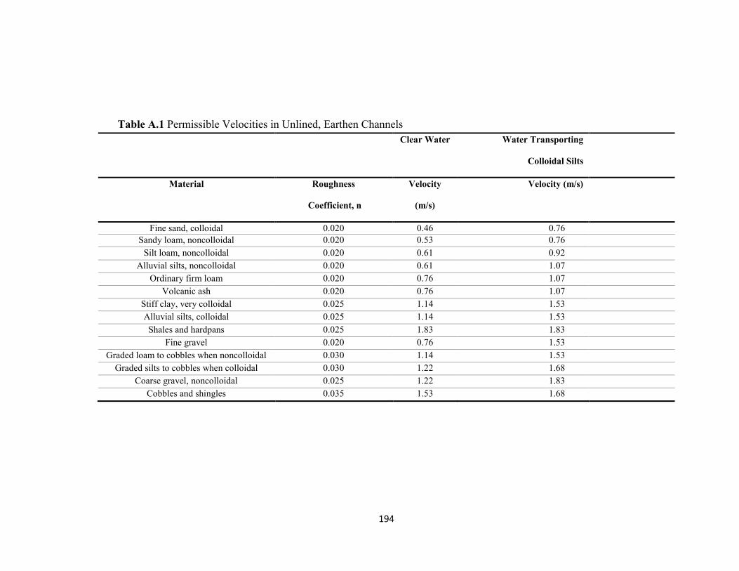
194
Table A.1 Permissible Velocities in Unlined, Earthen Channels
Clear Water Water Transporting
Colloidal Silts
Material Roughness
Coefficient, n
Velocity
(m/s)
Velocity (m/s)
Fine sand, colloidal 0.020 0.46 0.76 Sandy loam, noncolloidal 0.020 0.53 0.76
Silt loam, noncolloidal 0.020 0.61 0.92 Alluvial silts, noncolloidal 0.020 0.61 1.07
Ordinary firm loam 0.020 0.76 1.07 Volcanic ash 0.020 0.76 1.07
Stiff clay, very colloidal 0.025 1.14 1.53 Alluvial silts, colloidal 0.025 1.14 1.53 Shales and hardpans 0.025 1.83 1.83
Fine gravel 0.020 0.76 1.53 Graded loam to cobbles when noncolloidal 0.030 1.14 1.53
Graded silts to cobbles when colloidal 0.030 1.22 1.68 Coarse gravel, noncolloidal 0.025 1.22 1.83
Cobbles and shingles 0.035 1.53 1.68
195
APPENDIX B
GRAIN SIZE DISTRIBUTION
The grain size distribution (GSD) of the mixture which was used in this research is
presented in this section. The flume bed is covered with a mixture of sand and gravel,
including brown pea gravel circled, white limestone (coarsest), and dark basalt gravel
(intermediate size).
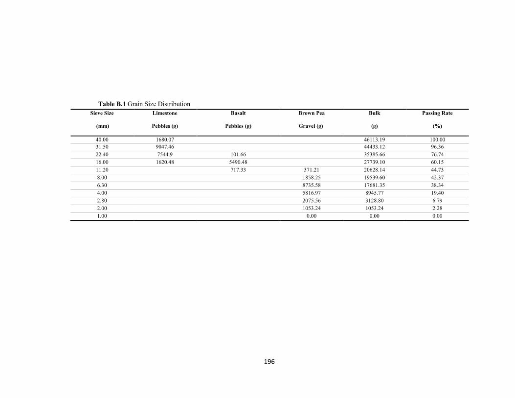
196
Table B.1 Grain Size Distribution
Sieve Size
(mm)
Limestone
Pebbles (g)
Basalt
Pebbles (g)
Brown Pea
Gravel (g)
Bulk
(g)
Passing Rate
(%)
40.00 1680.07 46113.19 100.00 31.50 9047.46 44433.12 96.36 22.40 7544.9 101.66 35385.66 76.74 16.00 1620.48 5490.48 27739.10 60.15 11.20 717.33 371.21 20628.14 44.73 8.00 1858.25 19539.60 42.37 6.30 8735.58 17681.35 38.34 4.00 5816.97 8945.77 19.40 2.80 2075.56 3128.80 6.79 2.00 1053.24 1053.24 2.28 1.00 0.00 0.00 0.00
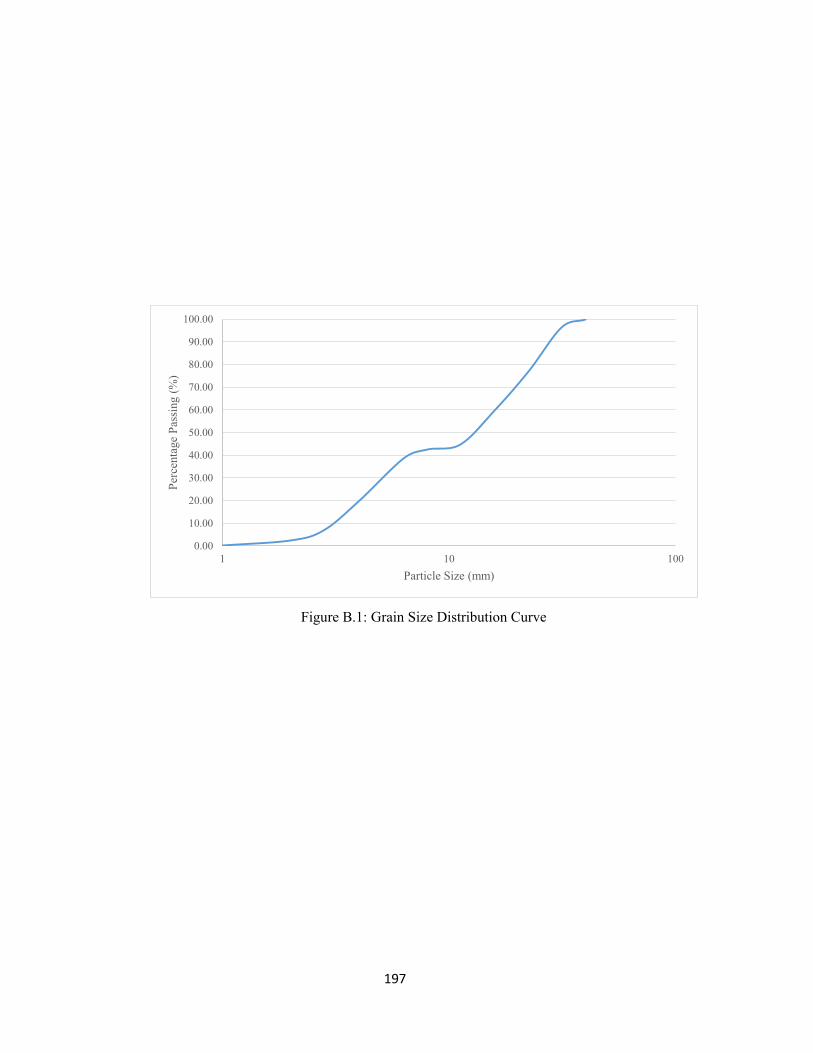
197
Figure B.1: Grain Size Distribution Curve
0.00
10.00
20.00
30.00
40.00
50.00
60.00
70.00
80.00
90.00
100.00
1 10 100
Perc
enta
ge P
assi
ng (%
)
Particle Size (mm)
198
APPENDIX C
EXPERIMENTAL MEASUREMENTS
Experimental measurements in vertical sluice gates are presented in Table C.1 and C.2 for
the main discharges and validation measurements. Gate opening, upstream depth,
downstream depth, downstream flow condition, the Flow Stability Factor, and the h0/a
ratio are reported in these tables.The data in these tables have been used in chapter three,
sections one and two, to show the experimental results and to also determine the Flow
Stability Number.
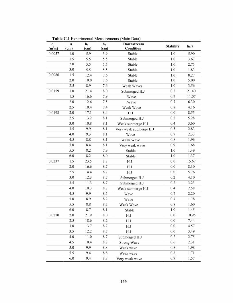
199
Table C.1 Experimental Measurements (Main Data) q (m2/s)
a (cm)
h0 (cm)
h1 (cm)
Downstream Condition Stability h0/a
0.0057 1.0 5.9 5.9 Stable 1.0 5.90 1.5 5.5 5.5 Stable 1.0 3.67 2.0 5.5 5.5 Stable 1.0 2.75 3.0 5.5 5.5 Stable 1.0 1.83 0.0086 1.5 12.4 7.6 Stable 1.0 8.27 2.0 10.0 7.6 Stable 1.0 5.00 2.5 8.9 7.6 Weak Waves 1.0 3.56 0.0159 1.0 21.4 8.0 Submerged H.J 0.2 21.40 1.5 16.6 7.9 Wave 0.7 11.07 2.0 12.6 7.5 Wave 0.7 6.30 2.5 10.4 7.4 Weak Wave 0.8 4.16 0.0198 2.0 17.1 8.4 H.J 0.0 8.55 2.5 13.2 8.1 Submerged H.J 0.2 5.28 3.0 10.8 8.1 Weak submerge H.J 0.4 3.60 3.5 9.9 8.1 Very weak submerge H.J 0.5 2.83 4.0 9.3 8.1 Wave 0.7 2.33 4.5 8.8 8.1 Weak Wave 0.8 1.96 5.0 8.4 8.1 Very weak wave 0.9 1.68 5.5 8.2 7.9 Stable 1.0 1.49 6.0 8.2 8.0 Stable 1.0 1.37 0.0237 1.5 23.5 8.7 H.J 0.0 15.67 2.0 16.6 8.7 H.J 0.0 8.30 2.5 14.4 8.7 H.J 0.0 5.76 3.0 12.3 8.7 Submerged H.J 0.2 4.10 3.5 11.3 8.7 Submerged H.J 0.2 3.23 4.0 10.3 8.7 Weak submerge H.J 0.4 2.58 4.5 9.9 8.5 Wave 0.7 2.20 5.0 8.9 8.2 Wave 0.7 1.78 5.5 8.8 8.2 Weak Wave 0.8 1.60 6.0 8.7 8.1 Stable 1.0 1.45 0.0270 2.0 21.9 8.0 H.J 0.0 10.95 2.5 18.6 8.2 H.J 0.0 7.44 3.0 13.7 8.7 H.J 0.0 4.57 3.5 12.2 8.7 H.J 0.0 3.49 4.0 11.0 8.7 Submerged H.J 0.2 2.75 4.5 10.4 8.7 Strong Wave 0.6 2.31 5.0 9.9 8.8 Weak wave 0.8 1.98 5.5 9.4 8.8 Weak wave 0.8 1.71 6.0 9.4 8.8 Very weak wave 0.9 1.57
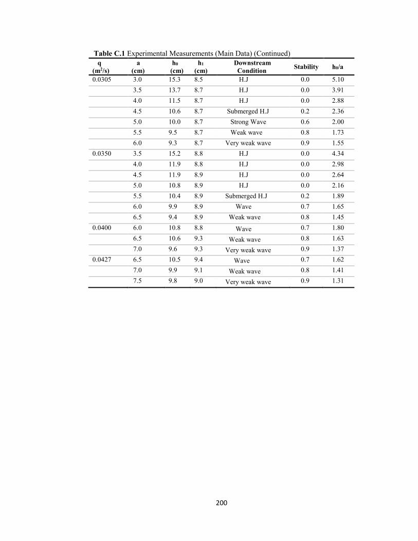
200
Table C.1 Experimental Measurements (Main Data) (Continued) q (m2/s)
a (cm)
h0 (cm)
h1 (cm)
Downstream Condition Stability h0/a
0.0305 3.0 15.3 8.5 H.J 0.0 5.10 3.5 13.7 8.7 H.J 0.0 3.91 4.0 11.5 8.7 H.J 0.0 2.88 4.5 10.6 8.7 Submerged H.J 0.2 2.36 5.0 10.0 8.7 Strong Wave 0.6 2.00 5.5 9.5 8.7 Weak wave 0.8 1.73 6.0 9.3 8.7 Very weak wave 0.9 1.55 0.0350 3.5 15.2 8.8 H.J 0.0 4.34 4.0 11.9 8.8 H.J 0.0 2.98 4.5 11.9 8.9 H.J 0.0 2.64 5.0 10.8 8.9 H.J 0.0 2.16 5.5 10.4 8.9 Submerged H.J 0.2 1.89 6.0 9.9 8.9 Wave 0.7 1.65 6.5 9.4 8.9 Weak wave 0.8 1.45 0.0400 6.0 10.8 8.8 Wave 0.7 1.80 6.5 10.6 9.3 Weak wave 0.8 1.63 7.0 9.6 9.3 Very weak wave 0.9 1.37 0.0427 6.5 10.5 9.4 Wave 0.7 1.62 7.0 9.9 9.1 Weak wave 0.8 1.41 7.5 9.8 9.0 Very weak wave 0.9 1.31
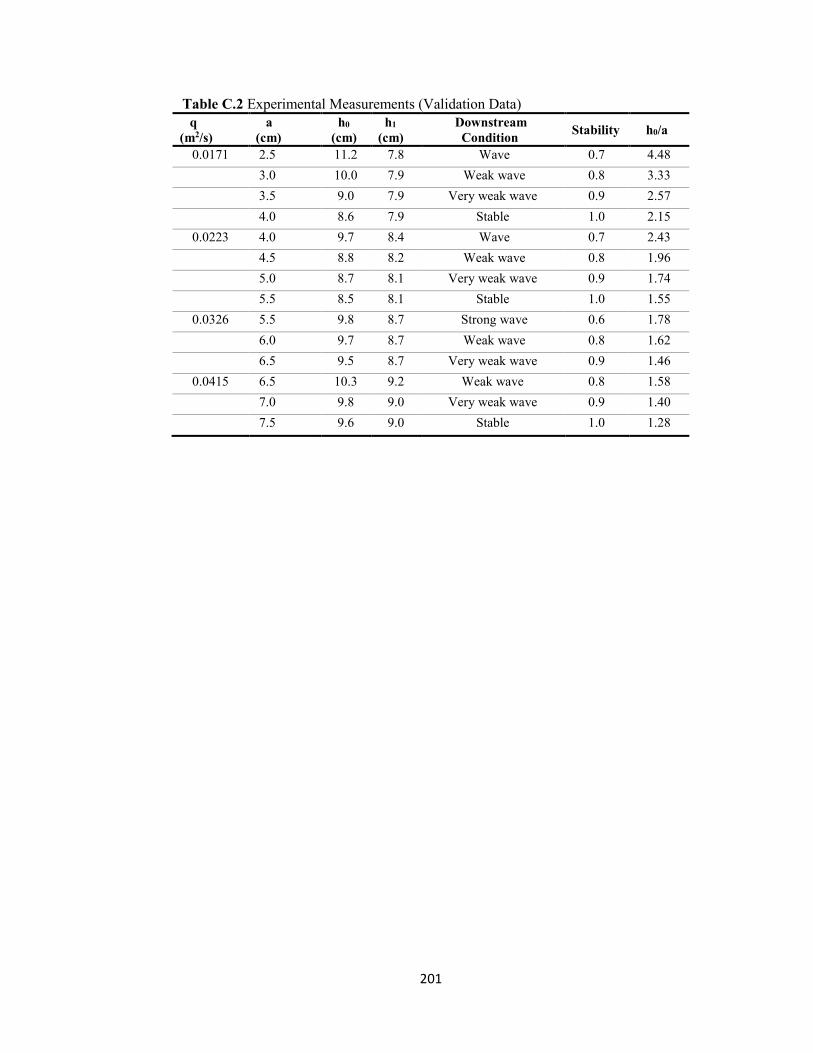
201
Table C.2 Experimental Measurements (Validation Data) q (m2/s)
a (cm)
h0 (cm)
h1 (cm)
Downstream Condition Stability h0/a
0.0171 2.5 11.2 7.8 Wave 0.7 4.48 3.0 10.0 7.9 Weak wave 0.8 3.33 3.5 9.0 7.9 Very weak wave 0.9 2.57 4.0 8.6 7.9 Stable 1.0 2.15
0.0223 4.0 9.7 8.4 Wave 0.7 2.43 4.5 8.8 8.2 Weak wave 0.8 1.96 5.0 8.7 8.1 Very weak wave 0.9 1.74 5.5 8.5 8.1 Stable 1.0 1.55
0.0326 5.5 9.8 8.7 Strong wave 0.6 1.78 6.0 9.7 8.7 Weak wave 0.8 1.62 6.5 9.5 8.7 Very weak wave 0.9 1.46
0.0415 6.5 10.3 9.2 Weak wave 0.8 1.58 7.0 9.8 9.0 Very weak wave 0.9 1.40 7.5 9.6 9.0 Stable 1.0 1.28
202
APPENDIX D
EXPERIMENTAL MEASUREMENTS
Experimental measurements for the vertical sluice gates for the first and second
laboratories are presented in Tables D.1 and D.2, respectively. Discharge, critical depth,
gate opening, upstream depth, downstream depth (section 2), downstream depth (section
3), upstream velocity, downstream velocity and energy (section 2), downstream velocity
and energy (section 3), and the Flow Stability Number are reported in this table. The data
in these tables have been used in chapter five, section two, for statistical analysis and to
determine the flow stability.
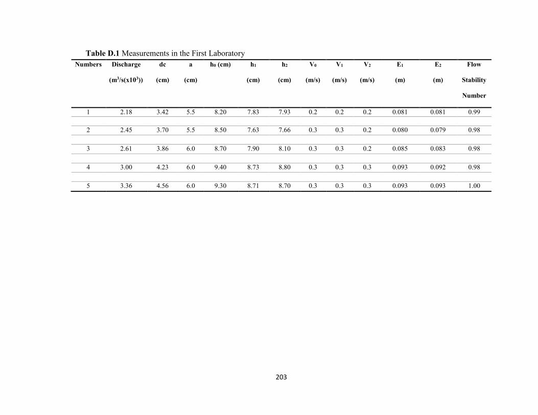
203
Table D.1 Measurements in the First Laboratory Numbers Discharge
(m3/s(x103))
dc
(cm)
a
(cm)
h0 (cm) h1
(cm)
h2
(cm)
V0
(m/s)
V1
(m/s)
V2
(m/s)
E1
(m)
E2
(m)
Flow
Stability
Number
1 2.18 3.42 5.5 8.20 7.83 7.93 0.2 0.2 0.2 0.081 0.081 0.99
2 2.45 3.70 5.5 8.50 7.63 7.66 0.3 0.3 0.2 0.080 0.079 0.98
3 2.61 3.86 6.0 8.70 7.90 8.10 0.3 0.3 0.2 0.085 0.083 0.98
4 3.00 4.23 6.0 9.40 8.73 8.80 0.3 0.3 0.3 0.093 0.092 0.98
5 3.36 4.56 6.0 9.30 8.71 8.70 0.3 0.3 0.3 0.093 0.093 1.00

204
Table D.1 Measurements in the First Laboratory (Continued) Numbers Discharge
(m3/s(x103))
dc
(cm)
a
(cm)
h0 (cm) h1
(cm)
h2
(cm)
V0
(m/s)
V1
(m/s)
V2
(m/s)
E1
(m)
E2
(m)
Flow
Stability
Number
6 3.58 4.76 6.5 9.50 8.60 8.70 0.3 0.4 0.3 0.095 0.094 0.99
7 3.86 5.01 6.5 9.40 8.78 8.90 0.4 0.4 0.3 0.097 0.095 0.97
8 4.43 5.49 7.0 9.60 8.86 9.10 0.4 0.5 0.4 0.099 0.097 0.96
9 4.56 5.60 7.5 9.60 8.91 9.00 0.4 0.5 0.4 0.102 0.098 0.96
10 4.70 5.71 7.5 9.80 8.93 9.00 0.4 0.5 0.4 0.102 0.099 0.97
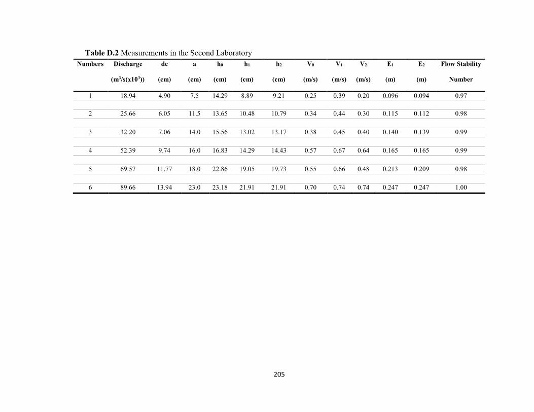
205
Table D.2 Measurements in the Second Laboratory Numbers Discharge
(m3/s(x103))
dc
(cm)
a
(cm)
h0
(cm)
h1
(cm)
h2
(cm)
V0
(m/s)
V1
(m/s)
V2
(m/s)
E1
(m)
E2
(m)
Flow Stability
Number
1 18.94 4.90 7.5 14.29 8.89 9.21 0.25 0.39 0.20 0.096 0.094 0.97
2 25.66 6.05 11.5 13.65 10.48 10.79 0.34 0.44 0.30 0.115 0.112 0.98
3 32.20 7.06 14.0 15.56 13.02 13.17 0.38 0.45 0.40 0.140 0.139 0.99
4 52.39 9.74 16.0 16.83 14.29 14.43 0.57 0.67 0.64 0.165 0.165 0.99
5 69.57 11.77 18.0 22.86 19.05 19.73 0.55 0.66 0.48 0.213 0.209 0.98
6 89.66 13.94 23.0 23.18 21.91 21.91 0.70 0.74 0.74 0.247 0.247 1.00
206
APPENDIX E
EXPERIMENTAL MEASUREMENTS
Experimental measurements in a gate with an expansion hydraulic system at the first and
second laboratories are presented in Tables E.1 to E.3 and E.4, respectively. Discharge,
critical depth, gate opening, upstream depth, downstream depth (section 2), downstream
depth (section 3), upstream velocity, downstream velocity and energy (section 2),
downstream velocity and energy (section 3), and the Flow Stability Number are reported
in this table. The data in these tables have been used in chapter five, section three, for
statistical analysis and to determine the flow stability.

207
Table E.1 Measurements, Thickness Two Centimeters Numbers Discharge
(m3/s(x103))
dc
(cm)
a
(cm)
h0
(cm)
h1
(cm)
h2
(cm)
V0
(m/s)
V1
(m/s)
V2
(m/s)
E1
(m)
E2
(m)
Flow
Stability
Number
1 2.18 3.42 5.5 9.17 7.87 7.90 0.2 0.3 0.3 0.082 0.082 1.00
2 2.45 3.70 5.5 10.07 7.97 7.97 0.2 0.3 0.3 0.084 0.084 1.00
3 2.61 3.86 6.0 9.87 7.87 7.85 0.2 0.3 0.3 0.083 0.083 1.00
4 3.00 4.23 6.0 10.67 7.96 8.00 0.3 0.3 0.3 0.085 0.084 0.98
5 3.36 4.56 6.0 11.57 7.77 8.08 0.3 0.5 0.4 0.090 0.089 0.98
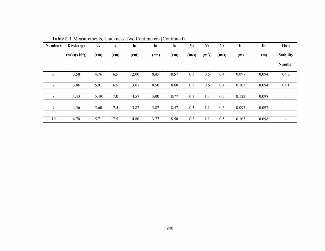
208
Table E.1 Measurements, Thickness Two Centimeters (Continued)
Numbers Discharge
(m3/s(x103))
dc
(cm)
a
(cm)
h0
(cm)
h1
(cm)
h2
(cm)
V0
(m/s)
V1
(m/s)
V2
(m/s)
E1
(m)
E2
(m)
Flow
Stability
Number
6 3.58 4.76 6.5 12.00 8.45 8.57 0.3 0.5 0.4 0.097 0.094 0.96
7 3.86 5.01 6.5 13.07 8.50 8.60 0.3 0.6 0.4 0.103 0.094 0.91
8 4.43 5.49 7.0 14.57 3.00 8.77 0.3 1.3 0.5 0.122 0.098 -
9 4.56 5.60 7.5 13.87 3.87 8.47 0.3 1.1 0.5 0.097 0.097 -
10 4.70 5.71 7.5 14.80 3.77 8.50 0.3 1.1 0.5 0.103 0.098 -
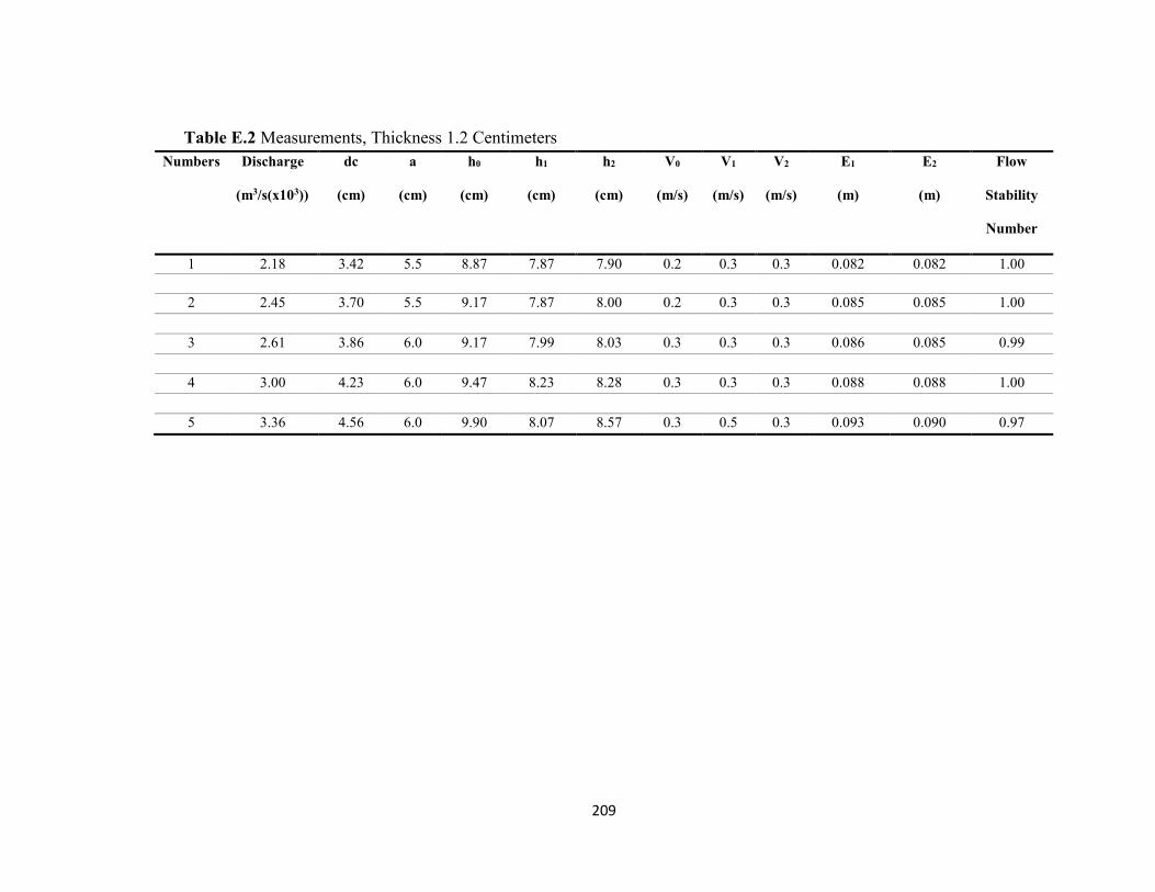
209
Table E.2 Measurements, Thickness 1.2 Centimeters
Numbers Discharge
(m3/s(x103))
dc
(cm)
a
(cm)
h0
(cm)
h1
(cm)
h2
(cm)
V0
(m/s)
V1
(m/s)
V2
(m/s)
E1
(m)
E2
(m)
Flow
Stability
Number
1 2.18 3.42 5.5 8.87 7.87 7.90 0.2 0.3 0.3 0.082 0.082 1.00
2 2.45 3.70 5.5 9.17 7.87 8.00 0.2 0.3 0.3 0.085 0.085 1.00
3 2.61 3.86 6.0 9.17 7.99 8.03 0.3 0.3 0.3 0.086 0.085 0.99
4 3.00 4.23 6.0 9.47 8.23 8.28 0.3 0.3 0.3 0.088 0.088 1.00
5 3.36 4.56 6.0 9.90 8.07 8.57 0.3 0.5 0.3 0.093 0.090 0.97
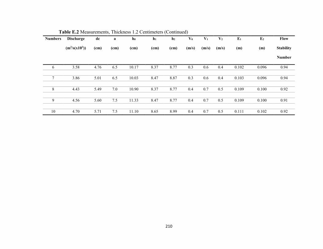
210
Table E.2 Measurements, Thickness 1.2 Centimeters (Continued) Numbers Discharge
(m3/s(x103))
dc
(cm)
a
(cm)
h0
(cm)
h1
(cm)
h2
(cm)
V0
(m/s)
V1
(m/s)
V2
(m/s)
E1
(m)
E2
(m)
Flow
Stability
Number
6 3.58 4.76 6.5 10.17 8.37 8.77 0.3 0.6 0.4 0.102 0.096 0.94
7 3.86 5.01 6.5 10.03 8.47 8.87 0.3 0.6 0.4 0.103 0.096 0.94
8 4.43 5.49 7.0 10.90 8.37 8.77 0.4 0.7 0.5 0.109 0.100 0.92
9 4.56 5.60 7.5 11.33 8.47 8.77 0.4 0.7 0.5 0.109 0.100 0.91
10 4.70 5.71 7.5 11.10 8.65 8.99 0.4 0.7 0.5 0.111 0.102 0.92
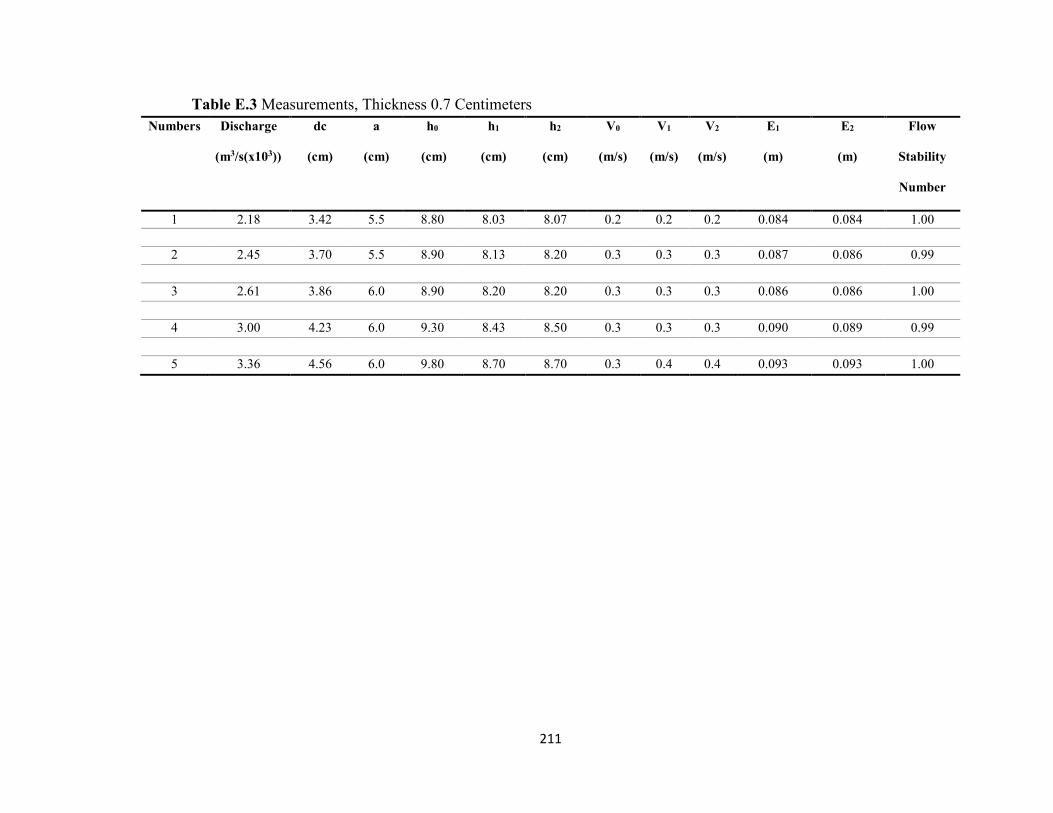
211
Table E.3 Measurements, Thickness 0.7 Centimeters Numbers Discharge
(m3/s(x103))
dc
(cm)
a
(cm)
h0
(cm)
h1
(cm)
h2
(cm)
V0
(m/s)
V1
(m/s)
V2
(m/s)
E1
(m)
E2
(m)
Flow
Stability
Number
1 2.18 3.42 5.5 8.80 8.03 8.07 0.2 0.2 0.2 0.084 0.084 1.00
2 2.45 3.70 5.5 8.90 8.13 8.20 0.3 0.3 0.3 0.087 0.086 0.99
3 2.61 3.86 6.0 8.90 8.20 8.20 0.3 0.3 0.3 0.086 0.086 1.00
4 3.00 4.23 6.0 9.30 8.43 8.50 0.3 0.3 0.3 0.090 0.089 0.99
5 3.36 4.56 6.0 9.80 8.70 8.70 0.3 0.4 0.4 0.093 0.093 1.00
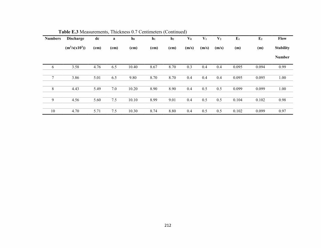
212
Table E.3 Measurements, Thickness 0.7 Centimeters (Continued) Numbers Discharge
(m3/s(x103))
dc
(cm)
a
(cm)
h0
(cm)
h1
(cm)
h2
(cm)
V0
(m/s)
V1
(m/s)
V2
(m/s)
E1
(m)
E2
(m)
Flow
Stability
Number
6 3.58 4.76 6.5 10.40 8.67 8.70 0.3 0.4 0.4 0.095 0.094 0.99
7 3.86 5.01 6.5 9.80 8.70 8.70 0.4 0.4 0.4 0.095 0.095 1.00
8 4.43 5.49 7.0 10.20 8.90 8.90 0.4 0.5 0.5 0.099 0.099 1.00
9 4.56 5.60 7.5 10.10 8.99 9.01 0.4 0.5 0.5 0.104 0.102 0.98
10 4.70 5.71 7.5 10.30 8.74 8.80 0.4 0.5 0.5 0.102 0.099 0.97
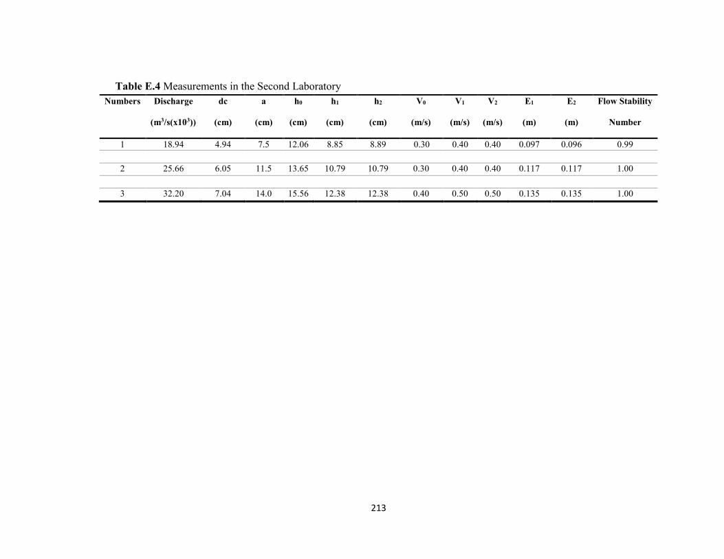
213
Table E.4 Measurements in the Second Laboratory
Numbers Discharge
(m3/s(x103))
dc
(cm)
a
(cm)
h0
(cm)
h1
(cm)
h2
(cm)
V0
(m/s)
V1
(m/s)
V2
(m/s)
E1
(m)
E2
(m)
Flow Stability
Number
1 18.94 4.94 7.5 12.06 8.85 8.89 0.30 0.40 0.40 0.097 0.096 0.99
2 25.66 6.05 11.5 13.65 10.79 10.79 0.30 0.40 0.40 0.117 0.117 1.00
3 32.20 7.04 14.0 15.56 12.38 12.38 0.40 0.50 0.50 0.135 0.135 1.00

214
APPENDIX F
EXPERIMENTAL MEASUREMENTS
Experimental measurements in a gate with a contraction hydraulic system at the first and
second laboratories are presented in Tables F.1 to F.3 and F.4, respectively. Discharge,
critical depth, gate opening, upstream depth, downstream depth (section 2), downstream
depth (section 3), upstream velocity, downstream velocity and energy (section 2),
downstream velocity and energy (section 3), and the Flow Stability Number are reported
in this table. The data in these tables have been used in chapter five, section four, for
statistical analysis and to determine the flow stability.
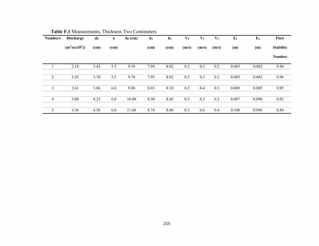
215
Table F.1 Measurements, Thickness Two Centimeters Numbers Discharge
(m3/s(x103))
dc
(cm)
a
(cm)
h0 (cm) h1
(cm)
h2
(cm)
V0
(m/s)
V1
(m/s)
V2
(m/s)
E1
(m)
E2
(m)
Flow
Stability
Number
1 2.18 3.42 5.5 9.10 7.94 8.02 0.2 0.3 0.2 0.085 0.082 0.96
2 2.45 3.70 5.5 9.70 7.95 8.02 0.2 0.3 0.2 0.085 0.082 0.96
3 2.61 3.86 6.0 9.80 8.03 8.10 0.2 0.4 0.3 0.089 0.085 0.95
4 3.00 4.23 6.0 10.80 8.50 8.60 0.3 0.5 0.3 0.097 0.090 0.92
5 3.36 4.56 6.0 11.60 8.74 8.80 0.3 0.6 0.4 0.108 0.096 0.89
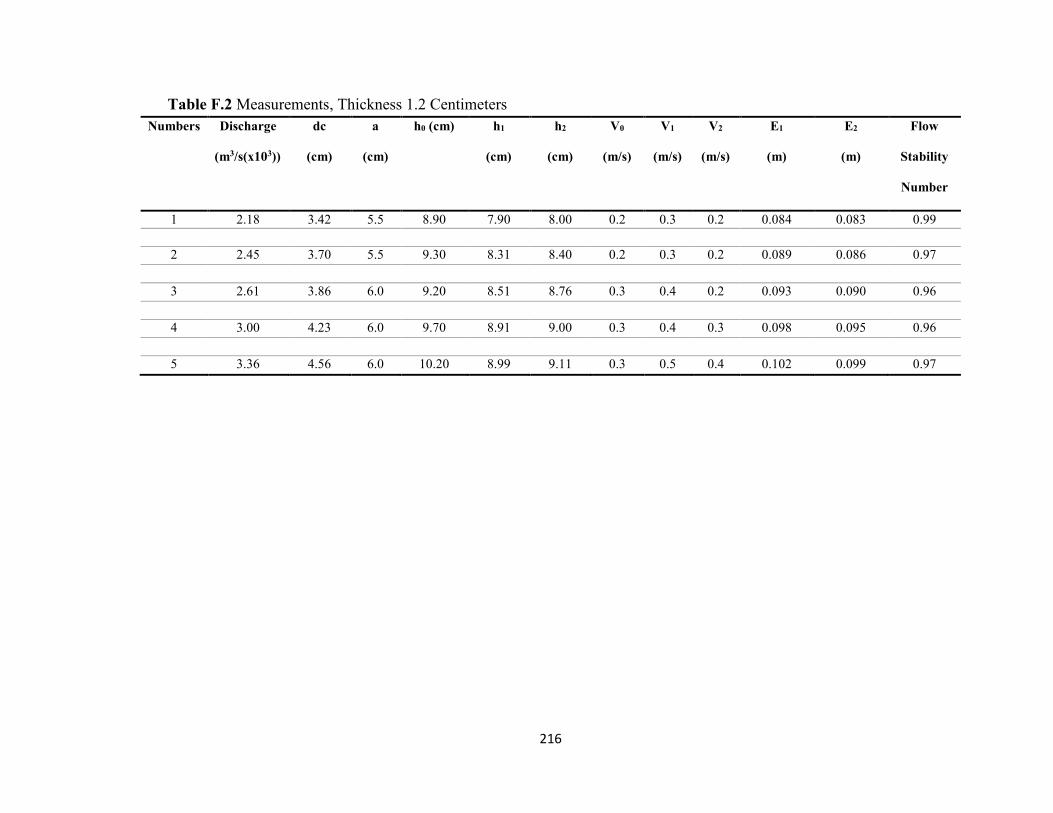
216
Table F.2 Measurements, Thickness 1.2 Centimeters Numbers Discharge
(m3/s(x103))
dc
(cm)
a
(cm)
h0 (cm) h1
(cm)
h2
(cm)
V0
(m/s)
V1
(m/s)
V2
(m/s)
E1
(m)
E2
(m)
Flow
Stability
Number
1 2.18 3.42 5.5 8.90 7.90 8.00 0.2 0.3 0.2 0.084 0.083 0.99
2 2.45 3.70 5.5 9.30 8.31 8.40 0.2 0.3 0.2 0.089 0.086 0.97
3 2.61 3.86 6.0 9.20 8.51 8.76 0.3 0.4 0.2 0.093 0.090 0.96
4 3.00 4.23 6.0 9.70 8.91 9.00 0.3 0.4 0.3 0.098 0.095 0.96
5 3.36 4.56 6.0 10.20 8.99 9.11 0.3 0.5 0.4 0.102 0.099 0.97
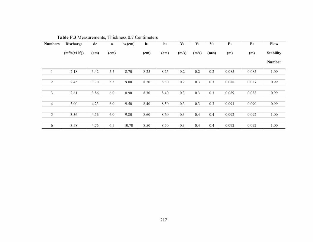
217
Table F.3 Measurements, Thickness 0.7 Centimeters
Numbers Discharge
(m3/s(x103))
dc
(cm)
a
(cm)
h0 (cm) h1
(cm)
h2
(cm)
V0
(m/s)
V1
(m/s)
V2
(m/s)
E1
(m)
E2
(m)
Flow
Stability
Number
1 2.18 3.42 5.5 8.70 8.25 8.25 0.2 0.2 0.2 0.085 0.085 1.00
2 2.45 3.70 5.5 9.00 8.20 8.30 0.2 0.3 0.3 0.088 0.087 0.99
3 2.61 3.86 6.0 8.90 8.30 8.40 0.3 0.3 0.3 0.089 0.088 0.99
4 3.00 4.23 6.0 9.50 8.40 8.50 0.3 0.3 0.3 0.091 0.090 0.99
5 3.36 4.56 6.0 9.80 8.60 8.60 0.3 0.4 0.4 0.092 0.092 1.00
6 3.58 4.76 6.5 10.70 8.50 8.50 0.3 0.4 0.4 0.092 0.092 1.00
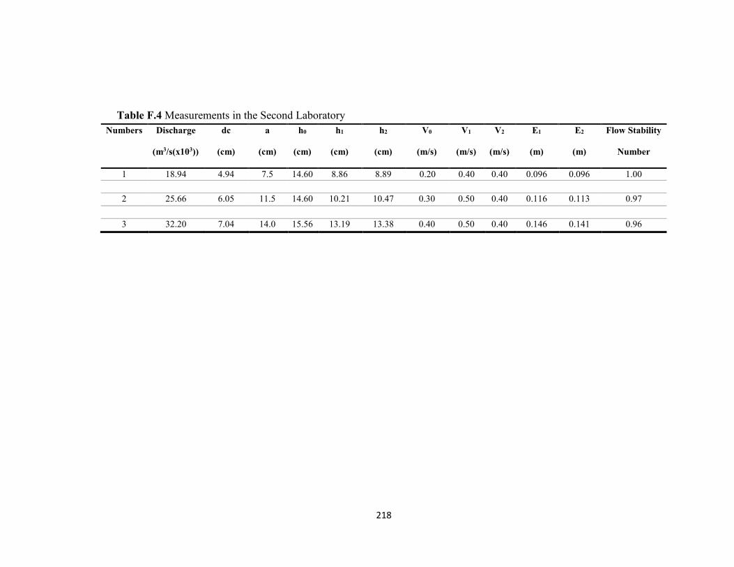
218
Table F.4 Measurements in the Second Laboratory Numbers Discharge
(m3/s(x103))
dc
(cm)
a
(cm)
h0
(cm)
h1
(cm)
h2
(cm)
V0
(m/s)
V1
(m/s)
V2
(m/s)
E1
(m)
E2
(m)
Flow Stability
Number
1 18.94 4.94 7.5 14.60 8.86 8.89 0.20 0.40 0.40 0.096 0.096 1.00
2 25.66 6.05 11.5 14.60 10.21 10.47 0.30 0.50 0.40 0.116 0.113 0.97
3 32.20 7.04 14.0 15.56 13.19 13.38 0.40 0.50 0.40 0.146 0.141 0.96

219
APPENDIX G
PROTOTYPE IMAGES
Pictures of the real-scale hydraulic structures (prototype) are provided in this section. The
structures are located in South Florida, Miami-Dade County.
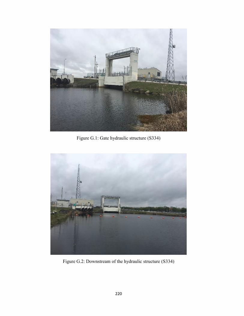
220
Figure G.1: Gate hydraulic structure (S334)
Figure G.2: Downstream of the hydraulic structure (S334)
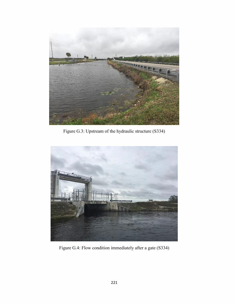
221
Figure G.3: Upstream of the hydraulic structure (S334)
Figure G.4: Flow condition immediately after a gate (S334)
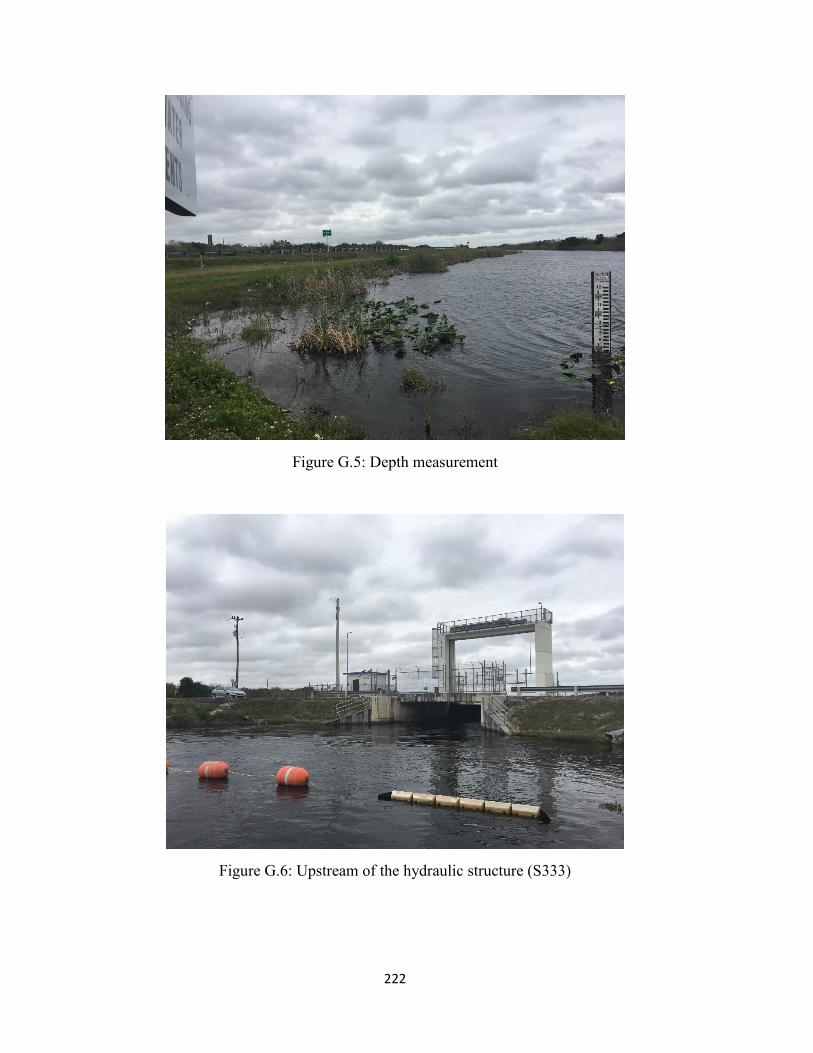
222
Figure G.5: Depth measurement
Figure G.6: Upstream of the hydraulic structure (S333)
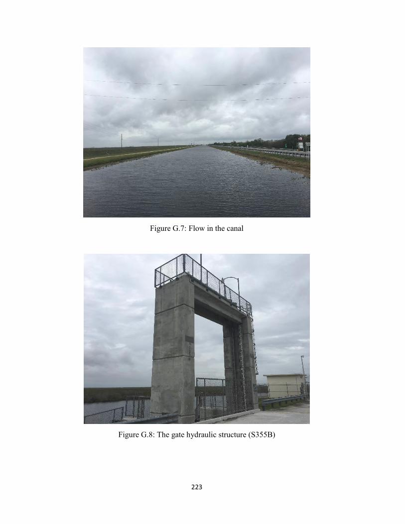
223
Figure G.7: Flow in the canal
Figure G.8: The gate hydraulic structure (S355B)
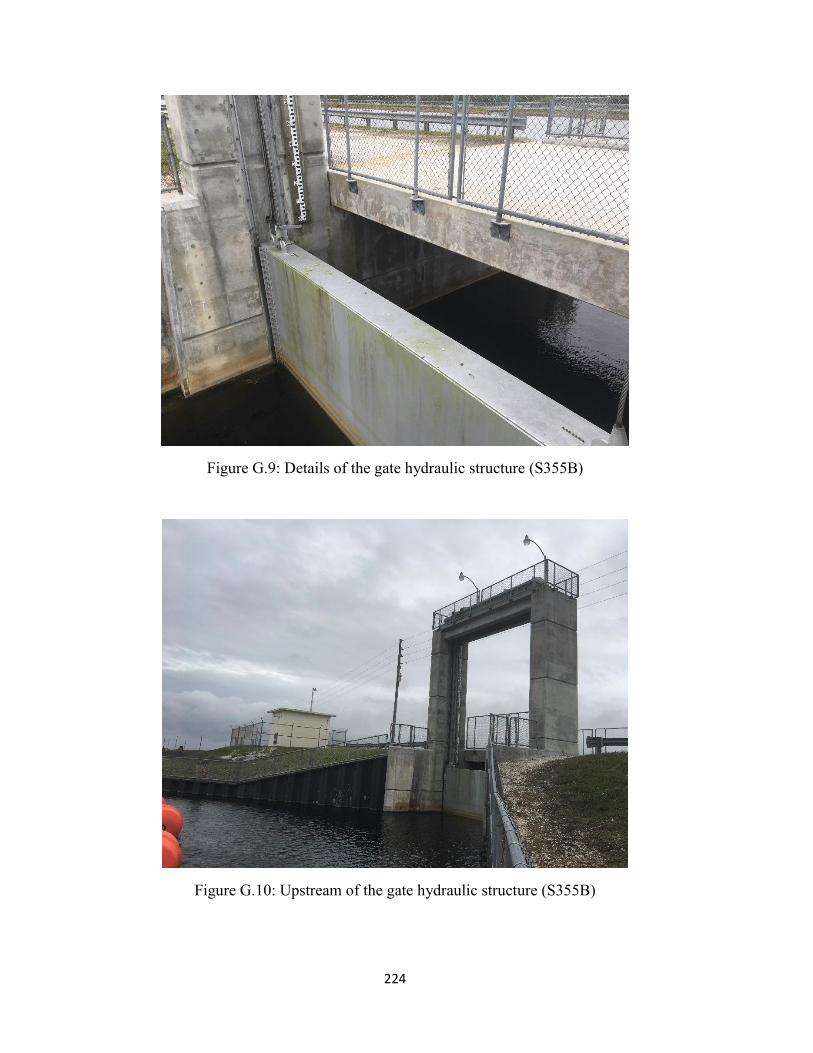
224
Figure G.9: Details of the gate hydraulic structure (S355B)
Figure G.10: Upstream of the gate hydraulic structure (S355B)
225
APPENDIX H
VALIDATION
The proposed method to determine the Efficiency Index that is documented in section 6 of
chapter 5 was validated with the results of the large physical model in the laboratory. The
validation data is reported in this section. The overall efficiency of the structure is the
difference between the total energies in the reservoir and the end of the stilling basin in
percentage terms.
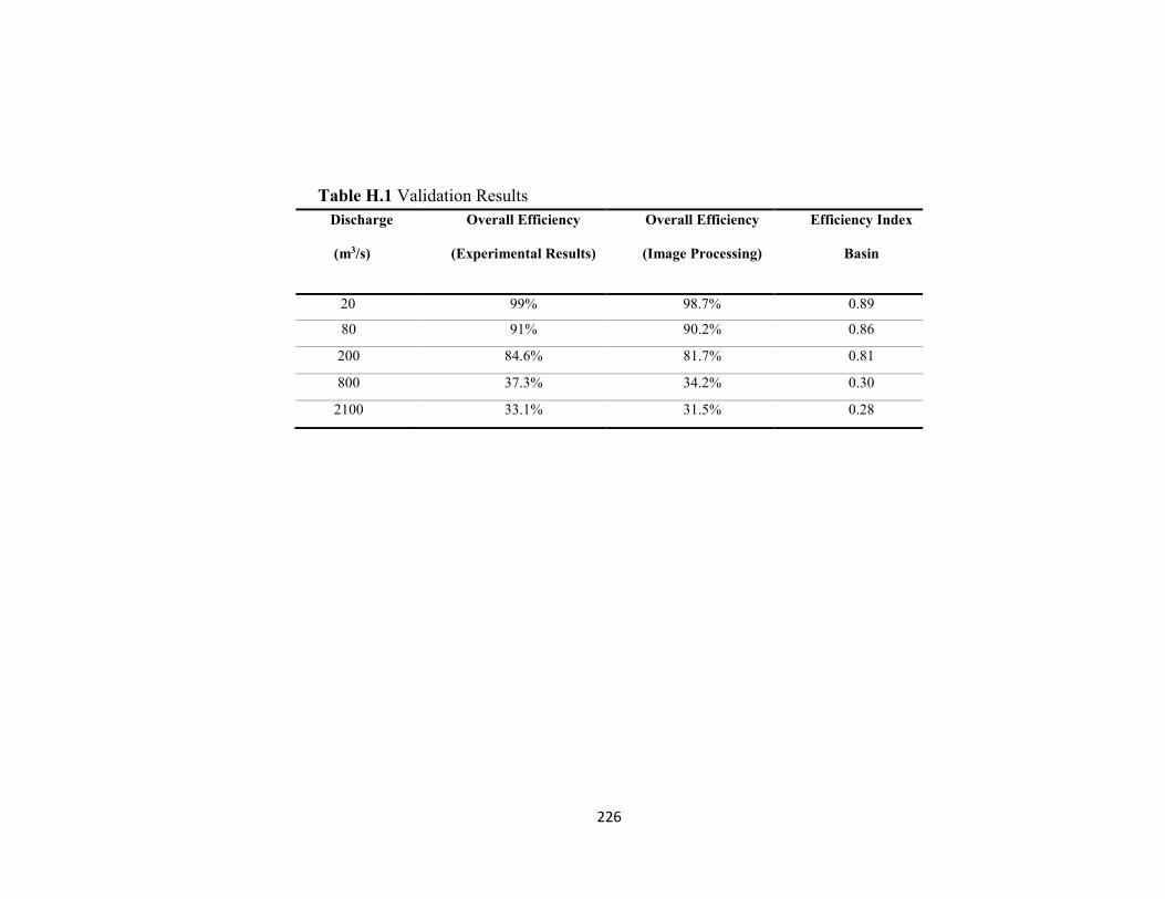
226
Table H.1 Validation Results
Discharge
(m3/s)
Overall Efficiency
(Experimental Results)
Overall Efficiency
(Image Processing)
Efficiency Index
Basin
20 99% 98.7% 0.89
80 91% 90.2% 0.86
200 84.6% 81.7% 0.81
800 37.3% 34.2% 0.30
2100 33.1% 31.5% 0.28
227
VITA
AMIRMASOUD HAMEDI
Born, Tehran, Iran
2002-2007 B.Sc., Civil Engineering
Azad University South Branch of Tehran
Tehran, Iran
2008-2010 M.Sc., Civil Engineering (Water Resources)
Azad University Central Branch of Tehran
Tehran, Iran
2014-2016 Research and Teaching Assistant
Florida International University
Miami, Florida
2014 -2017 PhD, Civil Engineering
Florida International University
Miami, Florida
PUBLICATIONS AND PRESENTATIONS*
Baqersad, M., Hamedi, A., Mohammadafzali, M., Ali, H., (2017). Asphalt Mixture
Segregation Detection: Digital Image Processing Approach. Advances in Material Science and Engineering. (doi.org/10.1155/2017/9493408)
*Hamedi, A., Fuentes, H.R., (2016) New Relationship between a Vertical Gate Opening
and Downstream Flow Stability: Experimental Development. World Environmental and Water Resources Congress, pp. 47–57.
228
Hamedi, A., Ketabdar, M., (2016). Energy Loss Estimation and Flow Simulation in the
Skimming Flow Regime of Stepped Spillways with Inclined Steps and End Sill: A Numerical
Model. International Journal of Science and Engineering Applications. 5(7), 399-407.
Hamedi, A., Haji Gholizadeh, M., Mansoori, A., (2016). Flow Simulation and Energy Loss
Estimation in the Nappe Flow Regime of Stepped Spillways with Inclined Steps and End
Sill: A Numerical Approach. Civil Engineering Journal. 2(9), 426-437.
Hamedi, A., Ketabdar, M., Hamedi, A., Fesharaki, M., Mansoori, A., (2016). Nappe Flow
Regime Energy Loss in Stepped Chutes Equipped with Reverse Inclined Steps:
Experimental Development. Florida Civil Engineering Journal. Volume 2, 28-37. ASCE-Florida Section.
Ketabdar, M., Hamedi, A., (2016). Intake Angle Optimization in 90-degree Converged
Bends in Presence of Floating Wooden Debris: Experimental Development. Florida Civil Engineering Journal. Volume 2, 22-27. ASCE-Florida Section.
Fesharaki, M., Hamedi, A., (2016). Effects of High-Speed Rail Substructure on Ground-
borne Vibrations. Florida Civil Engineering Journal. Volume 2, 38-47. ASCE-Florida Section.
Haji Gholizadeh, M., Hamedi, A., Niazi, A., & Eazi, M. (2016). Optimal Design of Water-
Supply Pipe Systems Using Economic and Technical Analysis. In World Environmental and Water Resources Congress. pp. 284-293.
*Hamedi, A., & Fuentes, H. R. (2015). Comparative Effectiveness and Reliability of
NEXRAD Data to Predict Outlet Hydrographs Using the GSSHA and HEC-HMS
Hydrologic Models. In World Environmental and Water Resources Congress. pp. 1444-1453.
Hamedi, A., Mansoori, A., Shamsai, A., Amirahmadian, S., (2014). The Effect of End Sill
and Stepped Slope on Stepped Spillway Energy Dissipation. Journal of Water Sciences Research. 6(1), 1-15.
Hamedi, A., Malekmohammadi, I., Mansoori, A., & Roshanaei, H. (2012). Energy
Dissipation in Stepped Spillway Equipped with Inclined Steps Together with End Sill. In Computational Intelligence and Communication Networks (CICN), Fourth International Conference. pp. 638-642. IEEE.
Hamedi, A., Mansoori, A., Malekmohamadi, I., & Roshanaei, H. (2011). Estimating
Energy Dissipation in Stepped Spillways with Reverse Inclined Steps and End Sill. In World Environmental and Water Resources Congress: Bearing Knowledge for Sustainability (pp. 2528-2537).


![Hydraulic Structures[4]](https://img.pdfslide.net/doc/110x75/563db7e1550346aa9a8ed1d4/hydraulic-structures4.jpg)