Embed Size (px)
Citation preview

Advanced Computer Graphics CS 563: Area and Environmental Light
William DiSanto
Computer Science Dept.Worcester Polytechnic Institute (WPI)

Outline
Radiometry Area Light Source Approximation Ambient Light Environmental Mapping Maps Explicit
Spherical Harmonics Irradiance Map

Radiometry
Radiance:
Irradiance:
Radiance [1]

Area Light Source
Approximation: Model the area light as point or directional For any or all area sources compute a single vector e
This vector represents the average magnitude and direction Irradiance can now be computed as
Light Vector [1]

Area Light Source: Alternatives
Easy to add color to the light vector model Wrapping: point light ‐> light that covers hemisphere
Implicit expression for a spherical area light Assuming constant radiance

Ambiance
Outgoing radiance take a simple constant term
Could replace with ambient reflectance for view dependent, self occluding ambiance

Environmental Mapping
Model reflective surfaces Project reflect vectors onto some function Use function evaluation as radiance
Environment Map [1]

EM: Maps Use components of reflect vector to sample:
Equirectangular: Two singularities at poles, does not preserve area
Mercator Equal Area [5]:
Other Maps:
[6]
[5]
[5][7]

EM: Sphere Mapping Use light probe or generate data in
View Dependent, recomputed for different view
Transform surface normal and view vector into reference frame of sphere map projection
[8]

EM: Cubic Environment Mapping View independent Better uniformity in sampling
Use isocube to achieve better distribution[1]
[9]

EM: Parabolic Mapping Join two parabolic projections No singularities Decent sampling Difficult to generate
[10]

EM: Glossy Reflections Artifacts from sampling cube map
Filter with Gaussian lobes at various resolutions Not accurate but gives appearance of variable reflectivity
[11]
[1] [11]

EM: Irradiance Mapping Map irradiance to some texture Generated from EM Addressed by the normal of surface
Generate Irradiance Map [1] [12]

Spherical Harmonics: Impetus
SH expression can allow for a reasonably accurate representation of low frequency objects.
Fast to compute, small set of polynomials Reasonably fast to solve Allow for frequency domain modification Functions are orthonormal

Spherical Harmonics : Description
Laplacian (divergence of gradient) expression.
Provides a frequency domain representation of some feature in spherical coordinates. We look for where this expression is 0. We will fit solutions to zeros of
the second derivative (essentially edge detection).

Spherical Harmonics: Expression
Two parts of the equation: Zonal (perturbed only in the altitude angle [0..PI])
Azimuthal (oscillates with altitude and azimuth) More components as frequency increases.
Real and imaginary components are identical but out of phase
Legendre Polynomial
Associated Legendre Polynomial

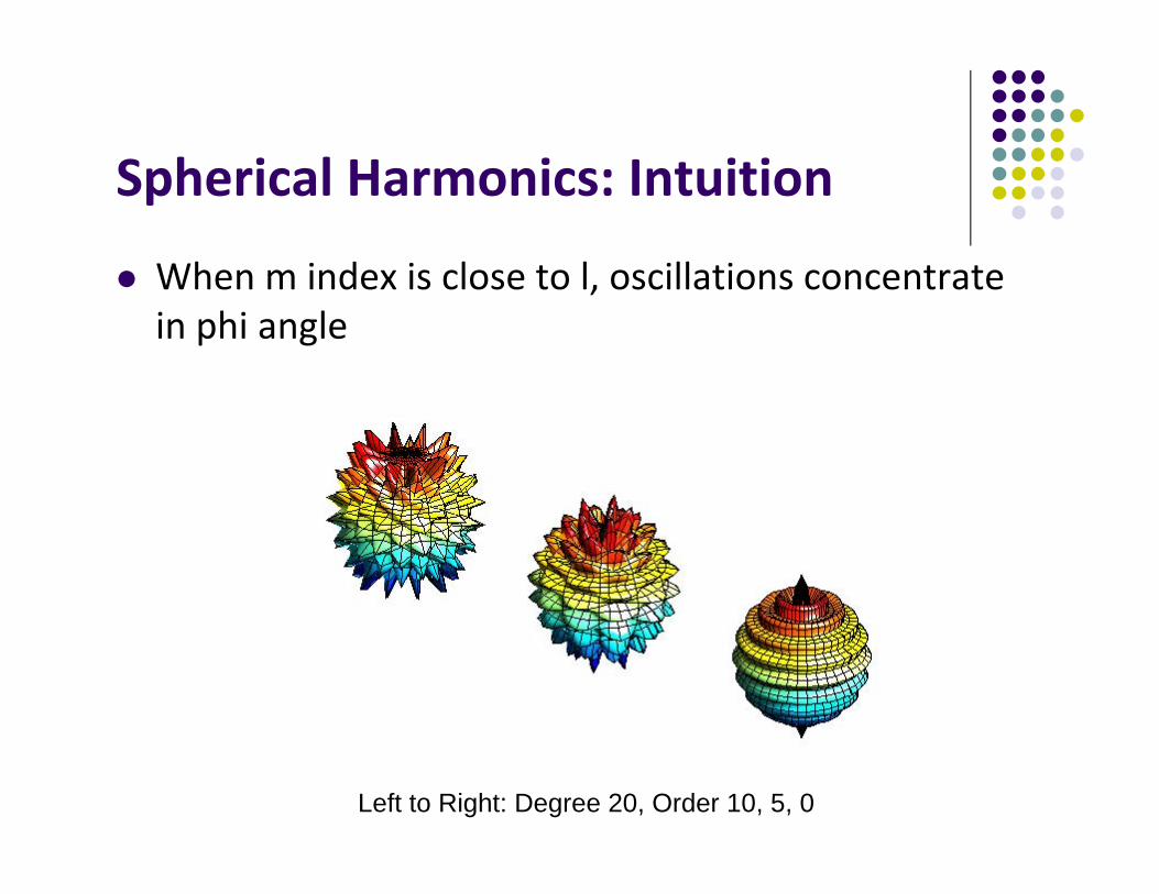
Spherical Harmonics: Intuition
As order index m approaches degree l, oscillations concentrate in theta angle
Left to Right: Degree 20, Order 10, 15, 20
Spherical Harmonics: Intuition
When m index is close to l, oscillations concentrate in phi angle
Left to Right: Degree 20, Order 10, 5, 0
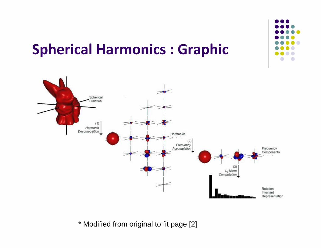
Spherical Harmonics : Graphic
* Modified from original to fit page [2]

Spherical Harmonics: Limitations
Requires many components to represent non‐axially symmetric data
Cannot represent all object perfectly, singularities require infinite terms
Is not necessarily rotation invariant however its power spectrum is rotation invariant

Spherical Harmonics: Solutions
Fit SH with least squares or some other method Build matrix of observed energy per Build matrix of basis functions constructed from
associated Legendre polynomials Use some fitting method to find function weights
Easy to generate with MATLAB, Mathematica, Boost libraries etc.
Some methods can solve in [4]

EM: Inexpensive Irradiance
Weighted sum of ground and sky radiance
Ambient cube
(x,y,z) irradiance selected from cube map surfaces within the hemisphere of surface normal
[3]

References [1] Real Time Rendering: Third Edition by [2] Michael Kazhdan , Thomas Funkhouser , Szymon Rusinkiewicz,
Rotation invariant spherical harmonic representation of 3D shape descriptors, Proceedings of the 2003 Eurographics/ACM SIGGRAPH symposium on Geometry processing, June 23‐25, 2003, Aachen, Germany
[3] Steven Parker , William Martin , Peter‐Pike J. Sloan , Peter Shirley , Brian Smits , Charles Hansen, Interactive ray tracing, Proceedings of the 1999 symposium on Interactive 3D graphics, p.119‐126, April 26‐29, 1999, Atlanta, Georgia, United States
[4] Rokhlin, V. and Tygert, M., Fast algorithms for spherical harmonic expansions, SIAM J. Sci.Comp. 27 (2005), 1903‐1928.
[5]http://mathworld.wolfram.com/SinusoidalProjection.html [6]http://earthobservatory.nasa.gov/Features/BlueMarble/

References [7]http://www.westnet.com/~crywalt/unfold.html [8]http://gl.ict.usc.edu/HDRShop/tutorial/tutorial5.html [9] Wan, L., Wong, T.‐T., and Leung, C.‐S. (2007). Isocube: Exploiting the Cubemap Hardware. IEEE Transactions on Visualization and
Computer Graphics, 13(4):720–731. [10] Wolfgang Heidrich , Hans‐Peter Seidel, Realistic, hardware‐
accelerated shading and lighting, Proceedings of the 26th annual conference on Computer graphics and interactive techniques, p.171‐178, July 1999
[11]http://developer.amd.com/archive/gpu/cubemapgen/pages/default.aspx
[12]http://http.developer.nvidia.com/GPUGems2/gpugems2_chapter10.html
http://www.mathworks.com/products/matlab/demos.html?file=/products/demos/shipping/matlab/spharm2.html


![CS 563 Advanced Topics in Computer Graphics Introduction To IBR By Cliff Lindsay Slide Show ’99 Siggraph[6]](https://img.pdfslide.net/doc/110x75/56649d7d5503460f94a5fe16/cs-563-advanced-topics-in-computer-graphics-introduction-to-ibr-by-cliff-lindsay.jpg)

![Computer Graphics (CS 563) 4: Advanced Computer Graphics … · 2012. 2. 8. · Microsoft PowerPoint - cs563_ibr_wk4_p2.ppt [Compatibility Mode] Author: emmanuel Created Date: 2/7/2012](https://img.pdfslide.net/doc/110x75/60afc1e8a784bf29d7469ece/computer-graphics-cs-563-4-advanced-computer-graphics-2012-2-8-microsoft.jpg)