Embed Size (px)
Citation preview
Internat. J. Math. & Math. Sci./oi.6 No.4 (1983) 671-703
671
ADVANCED DIFFERENTIAL EQUATIONS WITHPIECEWISE CONSTANT ARGUMENT DEVIATIONS
S.M. SHAHDepartment of Mathematics
University of KentuckyLexington, Kentucky 40502
and
JOSEPH WIENERDepartment of MathematicsPan American UniversityEdinburg, Texas 78539
(Received November 15, 1983)
ABSTRACT. Functional differential equations of advanced type with piecewise constant
argument deviations are studied. They are closely related to impulse, loaded and,
especially, to difference equations, and have the structure of continuous dynamical
systems within intervals of unit length.
KEY WORDS AND PHRASES. Functional Differential Equation, Advanced Equation,
Difference Equation, Piecewise Constant Deviation, Initial-Value Problem, Solution,
Existence, Uniqueness, Backward Continuation, Growth, Stability.
1980 MATHEMATICS SUBJECT CLASSIFICATION CODES. 34K05, 34K10, 34K20, 39A10.
i. INTRODUCTION.
In [i] and [2] analytic solutions to differential equations with linear trans-
formations of the argument are studied. The initial values are given at the fixed
point of the argument deviation. Integral transformations establish close connec-
tions between entire and distributional solutions of such equations. Profound links
exist also between functional and functional differential equations. Thus, the study
of the first often enables one to predict properties of differential equations of
neutral type. On the other hand, some methods for the latter in the special case
when the deviation of the argument vanishes at individual points has been used to
investigate functional equations [3]. Functional equations are directly related to
difference equations of a discrete (for example, integer-valued) argument, the theory
672 S.M. SHAH AND J. WIENER
of which has been very intensively developed in the book [4] and in numerous subse-
quent papers. Bordering on difference equations are also impulse functional differ-
ential equations with impacts and switching, loaded equations (that is, those inclu-
ding values of the unknown solution for given constant values of the argument),
equations
x’(t) f(t, x(t), x(h(t)))
with arguments of the form [t], that is, having intervals of constancy, etc. A sub-
stantial theory of such equations is virtually undeveloped [5]
In this article we study differential equations with arguments h(t) [t] and
h(t) [t+n], where [t] denotes the greatest-integer function. Connections are
established between differential equations with piecewise constant deviations and
difference equations of an integer-valued argument. Impulse and loaded equations
may be included in our scheme too. Indeed, consider the equation
x’(t) ax(t) + a0x([t ]) + alx([t+l])and write it as
x’(t) ax(t) + Y (a0x(i) + alx(i+l))(H(t-i) H(t-i-l)),i----
(i.l)
where H(t) i for t > 0 and H(t) 0 for t < 0. If we admit distributional deriva-
tives, then differentiating the latter relation gives
x"(t) ax’(t) + Z (aoX(i) + alx(i+l))((t-i) (t-i-l)),
where 6 is the delta functional. This impulse equation contains the values of the
unknown solution for the integral values of t. In the second section Eq. (I.I) is
considered. The initial-value problem is posed at t 0, and the solution is sought
for t > 0. The existence and uniqueness of solution and of its backward continuation
on (_oo, 0] is proved. Furthermore, an important fact is established that the initial
condition may be posed at any point, not necessarily integral. Necessary and suffi-
cient conditions of stability and asymptotic stability of the trivial solution are
determined explicitly via coefficients of the given equation, and oscillatory proper-
ties of solutions to (i.I) are studied.
In the third part the foregoing results are generalized for equations with many
deviations and systems of equations. We show that these equations are intrinsically
closer to difference rather than to differential equations. In fact, the equations
DIFFERENTIAL EQUATIONS WITH PIECEWISE CONSTANT ARGUMENT DEVIATIONS 673
considered in this paper have the structure of continuous dynamical systems within
intervals of unit length. Continuity of a solution at a point joining any two con-
secutive intervals then implies recursion relations for the solution at such points.
The equations are thus similar in structure to those found in certain "sequential-
continuous" models of disease dynamics as treated in [6]. We also investigate a
class of systems that depending on their coefficients combine either equations of
retarded, neutral or advanced type.
In the last section linear equations with variable coefficients are studied.
First, the existence and uniqueness of solution on [0, ) is proved for systems with
continuous coefficients. A simple algorithm of computing the solution by means of
continued fractions is indicated for a class of scalar equations. Then, a general
estimate of the solutions growth as t + is found. Special consideration is given
to the problem of stability, and for this purpose we employ a method developed
earlier in the theory of distributional and entire solutions to functional differen-
tial equations. An existence criterion of periodic solutions to linear equations
with periodic coefficients is established. Some nonlinear equations are also
tackled.
Consider the nth order differential equation with N argument delays
(m0x (t) f(t, x(t) x(mo-l)(t), x(t-Tl(t)) x(ml)(t-Tl(t))x(t-rN(t)) x(mN) (t-rN(t))), (1.2)
where all Ti(t) _> 0 and n max mi, 0 <_ i <_ N. Here x (k)(t-Ti(t)) is the kth deriva-
tive of the function x(z) taken at the point z t-Ti(t). Often equations that can
be reduced to the form (1.2) by a change of the independent variable are also dis-
cussed. A natural classification of functional differential equations has been
suggested in [7]. In Eq. (1.2) let max mi, i _< i _< N, and % m0 D. If % > 0,
then (1.2) is called an equation with retarded (lagging, delayed) argument. In the
case % O, Eq. (1.2) is of neutral type. For % < O, (1.2) is an equation of
advanced type. Retarded differential equations with piecewise constant delays (EPCD)
have been studied in [8, 9, i0]. Some results on neutral EPCD were announced in [9]
and [i0]. Together with the present paper, these works enable us to conclude that
all three types of EPCD share similar characteristics. First of all, it is natural
to pose the initial-value problem for such equations not on an interval but at a
674 S.M. SHAH AND J. WIENER
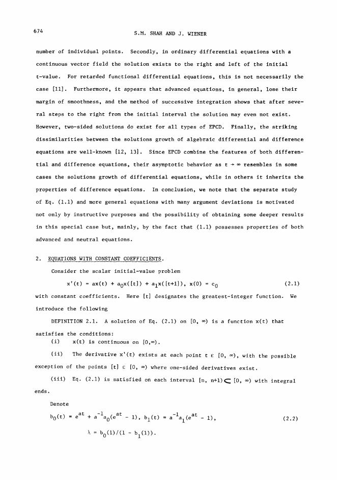
number of individual points. Secondly, in ordinary differential equations with a
continuous vector field the solution exists to the right and left of the initial
t-value. For retarded functional differential equations, this is not necessarily the
case [ll]. Furthermore, it appears that advanced equations, in general, lose their
margin of smoothness, and the method of successive integration shows that after seve-
ral steps to the right from the initial interval the solution may even not exist.
However, two-sided solutions do exist for all types of EPCD. Finally, the striking
dissimilarities between the solutions growth of algebraic differential and difference
equations are well-known [12, 13]. Since EPCD combine the features of both differen-
tial and difference equations, their asymptotic behavior as t resembles in some
cases the solutions growth of differential equations, while in others it inherits the
properties of difference equations. In conclusion, we note that the separate study
of Eq. (1.1) and more general equations with many argument deviations is motivated
not only by instructive purposes and the possibility of obtaining some deeper results
in this special case but, mainly, by the fact that (I.I) possesses properties of both
advanced and neutral equations.
2. EQUATIONS WITH CONSTANT COEFFICIENTS.
Consider the scalar initial-value problem
x’(t) ax(t) + a0x([t]) + alx([t+l]) x(0) co (2.1)
with constant coefficients. Here [t] designates the greatest-integer function. We
introduce the following
DEFINITION 2.1. A solution of Eq. (2.1) on [0, oo) is a function x(t) that
satisfies the conditions:
(i) x(t) is continuous on [0,oo).
(ii) The derivative x’(t) exists at each point t [0, oo), with the possible
exception of the points [t] e [0, o) where one-sided derivatives exist.
(iii) Eq. (2.1) is satisfied on each interval [n, n+l) C [0, oo) with integral
ends.
Denote
la0(eat -1 tb0(t) eat + a- i), bl(t) a al(e
ai), (2.2)
k b0(1)/(1 b1(1)).

DIFFERENTIAL EQUATIONS WITH PIECEWISE CONSTANT ARGUMENT DEVIATIONS 675
THEOREM 2.1. Problem (2.1) has on [0, oo) a unique solution
x(t) (bo({t}) + bl({t}))),It]cO, (2.3)
where {t} is the fractional part of t, if
bl(1) i. (2.4)
PROOF. Assuming that x (t) and x (t) are solutions of Eq. (2 l) on the inter-n n+l
vals [n, n+l) and [n+l, n+2), respectively, satisfying the conditions x (n) c andn n
Xn+l(n+l) Cn+l, we have
X’n(t) aXn(t) + a0cn + alCn+I, (2.5)
since Xn(n+l) Xn+l(n+l). The general solution of this equation on the given inter-
val is
x (t) ea(t-n)
a-I
c +n (a0Cn alcn+l)
with an arbitrary constant c. Putting here t n gives
-lao -1c (i + a )c + a
n alcn+land
Xn(t) b0(t-n)Cn + bl(t-n)cn+I (2.6)
For t n+l we have
Cn+l b0(1)Cn + bl(1)Cn+I, n _> 0
and inequality (2.4) implies
b0(1)Cn+l 1 bl(1) Cn
With the notations (2.2), this is written as
Cn+1 Xc n > 0.n
Hence,
%nc cn 0
This result together with (2.6) yields (2.3). Formula (2.3) was obtained with the
implicit assumption a # 0. If a 0, then
a0+ a
II + a
0x(t) (I +
i aI
{t})(l al)[t] Co’
which is the limiting case of (2.3) as a 0. The uniqueness of solution (2.3) on
[0 ) follows from its continuity and from the uniqueness of the problem x (n) cn n
for (2.5) on each interval [n, n+l]. It remains to observe that hypothesis (2.4) is
equivalent to
676 S.M. SHAH AND J. WIENER
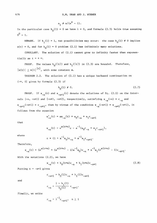
a # a/(ea I).1
In the particular case b0(1) 0 we have % 0, and formula (2.3) holds true assuming
00= i.
REMARK. If bl(1) i, two possibilities may occur: the case bo(1) # 0 implies
x(t) 0, and for b0(1) 0 problem (2.1) has infinitely many solutions.
COROLLARY. The solution of (2.1) cannot grow to infinity faster than exponen-
tially as t + .PROOF. The values b0({t}) and bl({t}) in (2.3) are bounded. Therefore,
ix(t) <_ mlll [t]with some constant m
THEOREM 2.2. The solution of (2.1) has a unique backward continuation on
(_oo, O] given by formula (2.3) if
b0(1) # 0. (2.7)
PROOF. If x (t) and x (t) denote the solutions of Eq. (2 I) on the inter--n -n+l
vals I-n,-n+l) and [-n+l,-n+2), respectively, satisfying x (-n) c and-n -n
X_n+l(-n+l) C_n+l, then by virtue of the condition X_n(-n+l) X_n+l(-n+l), it
follows from the equation
that
x’ (t) ax (t) + a0c +-n -n -n alC-n+l
x (t) ea(t+n) -i
c a (a0c + a Ic-n -n -n+l
where
-la0 -ic (l+a c +a
-n alC-n+lTherefore,
a(t+n) a-la0 -Ia
(t+n)x (t) (ea(t+n) + (e I) )c + a (ea-n -n i
l) C_n+l.
With the notations (2.2), we have
X_n(t) bo(t+n)C_n + bl(t+n)C-n+lPutting t -n+l gives
(2.8)
and
Finally, we write
Cun+l bO(1)c_n + b l(1)c_n+I
1 bI(I)C-n b
0(i) C-n+l
-ic =I c n> I-n -n+l
DIFFERENTIAL EQUATIONS WITH PIECEWISE CONSTANT ARGUMENT DEVIATIONS 6V7
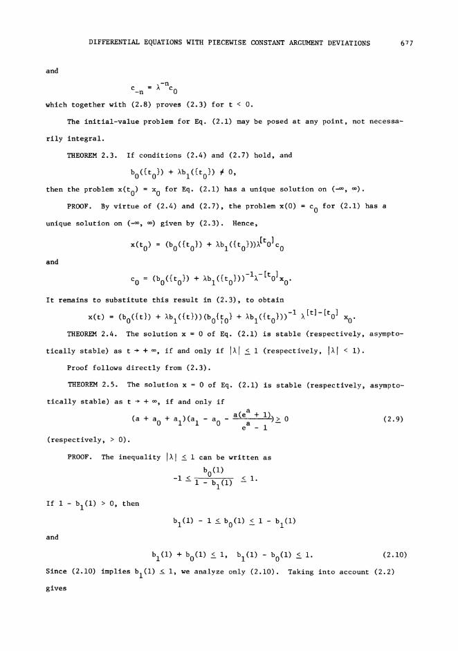
and
c %-nc0-n
which together with (2.8) proves (2.3) for t < 0.
The initial-value problem for Eq. (2.1) may be posed at any point, not necessa-
rily integral.
THEOREM 2.3. If conditions (2.4) and (2.7) hold, and
bo({t0}) + %bl({t0}) # 0,
then the problem x(t0) x0
for Eq. (2.1) has a unique solution on (_oo, ).
PROOF. By virtue of (2.4) and (2.7), the problem x(0) co for (2.1) has a
unique solution on (-co, oo) given by (2.3). Hence,
and
x(t0) (b0({t0}) + %bl({to}))%[tO]c0
co (b0({t0}) + %bl({t0}))-l%-[t0]XoIt remains to substitute this result in (2.3), to obtain
x(t) (b0({t}) + bl({t}))(b0{t0} + bl({t0})) -I [t]-[t0] xO.
THEOREM 2.4. The solution x 0 of Eq. (2.1) is stable (respectively, asympto-
tically stable) as t + oo, if and only if I%I _< i (respectively, I%I < i).
Proof follows directly from (2.3).
THEOREM 2.5. The solution x 0 of Eq. (2.1) is stable (respectively, asympto-
tically stable) as t + oo, if and only if
(a + a0+ al)(aI a
0
(respectively, > 0).
a(ea + i))_> 0a
e I(2.9)
PROOF. The inequality I%1 <_ i can be written as
bo(1)< I.I bI(I)
If I bl(1) > O, then
and
bI(I) i <_ b0(I) <_ I bI(I)
bl(1) + b0(1) < i, bl(1) b0(1) < i. (2.10)
Since (2.10) implies bl(1) <_ i, we analyze only (2.10). Taking into account (2.2)
gives

6 78 S .M. SHAH AND J. WIENER
-iea -i
a al(ea i) + + a a0(ea
i) <_ I,
-i a -iea
a al(ea
i) e a a0( I) < i.
From here, we have
-iea a
a (a0+ al)( i) < i- e
that is,
a + a0+ aI _< 0,
and
-ia (aI a0)(ea i) <_ e
a + i
which is equivalent to
a(ea + i) < 0al- ao- a
e i
(2.11)
(2.12)
If I bI(I) < 0, then
bl(1) + b0(1) > i, bl(1) b0(1) _> 1.
These inequalities imply b1(1) > 1. Therefore, we consider only
-lal(ea ea a-la0 eaa i) + + i) _> i,
-I a -iea
a al(ea
i) e a a0( i) _> I.
These relations yield inequalities opposite to (2.11) and (2.12) and prove the theorem
COROLLARY. The solution x 0 of the equation
x’(t) ax(t) + a0x([t])is stable (asymptotically stable) iff the inequalities
-a(ea + l)/(ea i) <_ a0 <_- a
(strict inequalities) take place.
(2.13)
THEOREM 2.6. In each interval (n, n+l) with integral ends the solution of Eq.
(2.1) with the condition x(O) c
if
# 0 has precisely one zero0a0+ alea
t =n+l/nn a a+a0+aI
a
(a0 + aae )(al aa > 0. (2.14)e i e i
If (2.14) is not satisfied and a0
# -aea/(ea i), co # O, then solution (2.3) has no
zeros in [0,

DIFFERENTIAL EQUATIONS WITH PIECEWISE CONSTANT ARGUMENT DEVIATIONS 679
PROOF. For # 0, cO # O, the equation x(t) 0 is equivalent to
bo({t}) + %bl({t}) O.
Hence,
and
bo({t})/bl({t}) bo(1)/(bl(1) I)
ea{t) + a-lao(ea(t)
-I (ea(t}a aI i)
a a-la0
eai) e + l)
-ial(ea- i) ia
It follows from here that
a{t}e (a
0+ alea)/(a + a
0 + al).If a > 0, then
alea a0ai < (a
0+ /(a + + aI) < e
and, by virtue of (2.4), the equality sign on the left must be omitted. The case
a+ao+al>0 (2.15)
leads to
a0
> aea/(ea i), aI> a/(ea i).
By adding inequalities (2.16) it is easy to see that (2.15) is a consequence of(2.16). If
(2.16)
then
and
a > 0, a + a0 + aI< 0,
ea
(a + a0 + aI) < a
0+ alea < a + a
0+
a0<- aea/(ea i), aI
< a/(ea
i). (2.17)
Again, the inequality a + a0+ aI
< 0 follows from (2.17). The case a < O, together
with (2.4), gives
a ae < (a
0+ ale )/(a + a
0+ aI) < I,
and assumption (2.15) yields (2.16). And if a + a0+ aI
< 0, then we obtain (2.17).
Hypothesis (2.14) can also be written as b0(1)(bl(1) i) > 0 which is equivalent to
k<O.
COROLLARY. In each interval (n, n+l) the solution
a0 a0 a0 a0 [t]x(t) (ea{t}(l +- - )(ea(l +- - cO
(2.18)
of (2.13) satisfying the condition x(0) co 0 has precisely one zero

680 S.M. SHAH AND J. WIENER
if
a0
t =n+llnn a a+a
0
a0
< aea/(ea i).
If (2.19) is not satisfied, solution (2.18) has no zeros in [0, ).
(2.19)
From the last two theorems we obtain the following decomposition of the space
(a, ao, al).i. If
aae a(e
a + i) > 0,(a0+ a
0a (al ae -I e -i
(2.20)
solution (2.3) with cO # 0 has precisely one zero in each interval (n, n+l) and
lira x(t) 0 as t / + o.
In fact, the solution possesses the required properties iff -I < % < O, that is
%(% + i) < O. With the notations (2.2), we have bo(1)(bo(1) bl(1) + i) < 0 which
yields (2.20).
2. If(a + a
0 + al)(a0 + aea< 0, (2.21)
e 1solution (2.3) with cO # 0 has no zeros in (0, ) and lim x(t) 0 as t + .
The properties take place iff 0 < % < i. Hence, we consider the inequality
%(% i) < 0 leading to (2.21).
3. If
a a(ea + i) < 0, (2.22)(aI a
0a (al ae I e i
solution (2.3) with cO # 0 has precisely one zero in each interval (n, n+l) and is
unbounded on [0, ).
The proof follows from the inequality % < i which is equivalent to (bl(1) i)
(bl(l -b0(1) I) < 0 and gives (2.22).
4. If
a < 0, (2 23)(a + a0+ al)(aI a
e i
solution (2.3) with co # 0 has no zeros in (0, oo) and is unbounded.
Relation (2.23) results from % > i which can be written as (bl(1) l)(b0(1) +
bI(I) i) < 0.

DIFFERENTIAL EQUATIONS WITH PIECEWISE CONSTANT ARGUMENT DEVIATIONS 681
5. If aI a0
a(eaa + i) O, a0 + aaeae I e i
# 0, solution (2.3) with co # 0
has precisely one zero in each interval (n, n+l) and is bounded on [0, oo) (but does
not vanish as t m) since, in this case, % -i.aa(ea + i) ae
0, a0+6. If aI a0 a a
e i e i0, then aI a/(ea i), and
problem (2.1) has infinitely many solutions.
7. If a + a0+ aI 0, aI # a/(ea I), then x(t) co Indeed, here we have
% i and
-i ea{t}x(t) (b0({t}) + bl({t}))c0 a (a + a0+ aI) a
0 al)c0.
8. Finally, if a0+
aae a
=0, a1a a
e i e I# 0, then x(t) b0(t)c0, for
0 <_ t < I, and x(t) 0, for t >_ i.
For Eq. (2.13) we have the following decomposition of the plane (a, a0).i. If -a(e
a + l)/(ea i) < a0
< -aea/(ea i), solution (2.18) with c0
0 has
precisely one zero in each interval (n, n+l) and lim x(t) 0 as t
2. If -aea/(ea i) < a0
< -a, then x(t) has no zeros in (0, oo) and lim x(t)
0 as t /o.
3. For a0<-a(ea + l)/(e
ai) the solution has precisely one zero in each
interval (n, n+l) and is unbounded on [0, oo).
4. For a0
> -a the solution has no zeros in (0, oo) and is unbounded.
a aThe case a
0-a yields x(t) co If a
0-ae /(e I), then x(t) bo(t)c0
on [0, I), and x(t) 0 on [i, ). For a0
-a(ea + l)/(ea
i) the solution x(t)
if bounded and oscillatory.
3. SOME GENERALIZATIONS.
For the problem
x’(t) Ax(t) + A0x([t]) + AlX([t+l]), x(0) coin which A, A0, AI
are r x r matrices and x is an r-vector, let
B0(t) eAt + (eAt I)A-IA0 Bl(t) (eAt I)A-IAI.
THEOREM 3.1. If the matrices A and I BI(1) are nonsingular, then problem
(3.1) has on [0, ) a unique solution
(3.1)
682 S.M. SHAH AND J. WIENER
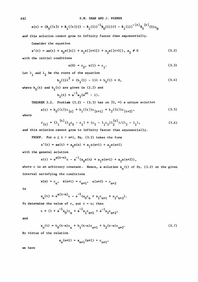
x(t) (B0({t}) + Bl({t})(I BI(1))-IBo(1))(I Bl(1))-[t]B0[t](1)c0and this solution cannot grow to infinity faster than exponentially.
Consider the equation
x’(t) ax(t) + a0x([t]) + alx([t+l]) + a2x([t+2]), a2 # 0
with the initial conditions
(3.2)
x(O) co x(1) c1.
Let hI and 2 be the roots of the equation
b2(1)%2 + (bl(1) i) + b0(1) 0,
where b0(t) and bl(t) are given in (2.2) and
-i (eatb2(t) a a2 i).
THEOREM 3.2. Problem (3.2) (3.3) has on [0, oo) a unique solution
(3.3)
(3.4)
x(t) 50({t})c[t + bl({t})c[t+l + b2({t})c[t+2], (3.5)
where
It] [t]c[t] (hi (2c0 Cl) + (Cl %1c0)2 )/(2 hi)’ (3.6)
and this solution cannot grow to infinity faster than exponentially.
PROOF. For n < t < n+l, Eq. (3.2) takes the form
x’(t) ax(t) + a0x(n) + alx(n+l + a2x(n+2with the general solution
x(t) ea(t-n)
a-I
c (a0x(n) + alx(n+l) + a2x(n+2))where c is an arbitrary constant. Hence, a solution x (t) of Eq. (3.2) on the given
n
interval satisfying the conditions
x(n) Cn, x(n+l) en+l, x(n+2) Cn+2is
x (t) ea (t-n) -I
nc a (a0cn + alCn+I + a2Cn+2).
To determine the value of c, put t n; then
-la0 -i -ic (i + a c + a + a a
n alcn+l 2Cn+2and
Xn(t) b0(t-n)cn + bl(t-n)cn+I + b2(t-n)cn+2.By virtue of the relation
(3.7)
x (n+l) (n+l)n Xn+l Cn+l
we have
DIFFERENTIAL EQUATIONS WITH PIECEWISE CONSTANT ARGUMENT DEVIATIONS 683
whence
Cn+l b0(1)Cn + bl(1)Cn+I + b2(1)Cn+2
b2(1)Cn+2 + (bl(1) l)Cn+I + b0(1)c 0 n > 0 (3 8)n
We look for a nontrivial solution of this difference equation in the form c xn.n
Then
b2 (1)In+2 + (bl(1) 1)Xn+l + b0(1)Xn
0,
and X satisfies (3.4). If the roots 1 and X2 of (3.4) are different, the general
solution of (3.8) is
n nc kilI + k212n
with arbitrary constants kI and k2. In fact, it satisfies (3.8) for all integral n.
In particular, for n 0 and n 1 this formula gives
k1+ k
2cO IlkI + X2k2 c1,
and
kI (%2c0- Cl)/(%2 %1), k2
(c I %ic0)/(%2- %1).These results, together with (3.7), establish (3.5) and (3.6).
If %1-- %2 l, then
c It] I It-l](c l[t] %Co[t-l])
which is the limiting case of (3.6) as %2 / %1" Formula (3.5) was obtained with the
implicit assumption a # 0. If a 0, then
x(t) c[t + (a0c[t + alc[t+l + a2c[t+2]){t},which is the limiting case of (3.5) as a 0. The uniqueness of solution (3.5) on
[0, m) follows from its continuity and from the uniqueness of the coefficients cn
for each n >_ 0. The conclusion about the solution growth is an implication of the
estimates for expressions (3.6).
THEOREM 3.3. If b0(l # 0, the solution of (3.2) (3.3) has a unique backward
continuation on (-oo, O] given by (3.5) (3.6).
Theorem 2.3 establishes an important fact that the initial-value problem for Eq.
(2.1) may be posed at any point, not necessarily integral. A similar proposition is
true also for Eq. (3.2).
THEOREM 3.4. If b0 (I) # 0 and
280 + (1- bl(1))8081 + ((1 bl(1))
22b0(i))8082
2 2 2+ b0(1)81 + b0(1)(l bi(i))8182 + b0(1)B 2# 0, (3.9)

684
where
S.M. SHAH AND J. WIENER
B0 b0({t0})’ B1 bl({t0})’ B2 b2({t0})’then the initial-value problem x(t0) x0, x(t
0 + i) xI for (3.2) has a unique
solution on (-oo,
PROOF. With the notation
(t) (ht][
i )l(h2we obtain from (3.6) the equations
c[t0+i] =-b0(1)(t0-1+i)c0 + (t0+i)cl, i 0, i, 2, 3.
Substituting these values in (3.5) for t tO and t to + 1 and taking into account
{to + i} {to gives the system
(-b0(1)((t0 I)B0+ (to)BI + (t0
+ i)2)c0 +
+ ((t0)B0 + #(t0+ i)
i+ #(t0 + 2)B2)cI Xo,
(-b0(1)((t0)0 + #(t0+ i)
i+ (t0 + 2)2)c0 + (3.i0)
+ ((t0+ I)
0 + (t0+ 2)BI + (t0 + 3)B2)cI x
I
for the unknowns co and cI. Computations show that
(t0+ m) (t + n)
0 -(b0(I)) [t0]+n+p-m(h-P(t0
+ p) (t0 + n + p m)
m-p) h-n m-n 2hi
)/(h2 hi)
for any integers m, n, p. This result leads to the conclusion that the determinant
of (3.10) coincides with the left-hand side of (3.9). Hence, we can express the
coefficients co and cI via the initial values x0
and xI and substitute in (3.5) and
(3.6), to find the solution x(t).
THEOREM 3.5. The solution x 0 of Eq. (3.2) is stable (respectively, asympto-
tically stable) as t + , if and only if lhl < i (respectively, lhl < i), i 1,2.
Proof follows from (3.6) and from the boundedness of the values b.({t}).
THEOREM 3.6. The solution x 0 of Eq. (3.2) is asymptotically stable if
a
(a0 +aae
)a2
< 0e 1
(3.11)
and either of the following hypotheses is satisfied:
(i) (a + a0 + aI + a2)(aI
a)<0,a
e 1
DIFFERENTIAL EQUATIONS WITH PIECEWISE CONSTANT ARGUMENT DEVIATIONS 685
a(ea + i) < 0,(ii) (aIa )(_ ao + al a2a a
e I e -i
where the first factors in (i) and (ii) retain the sign of a2.
PROOF. With the notations b. b.(1), it follows from (3.11) that
D2
(1 bl)2 4b0b2> O,
hence the roots
hi, 2(I- bI
+ D)/2b2
of (3.4) are real. If a2
> 0, the inequalities I%iI < 1 are equivalent to
and
i bI + D < 2b
2(3.12)
I bI
D > 2b2.
From (3.12) we obtain
(3.13)
and (3.13) yields
bI + 2b
2> I, b
0+ b
I + b2
> I,
bI 2b
2< i, b
0+ b
Ib2
< I.
The inequalities bI + 2b
2< b
0+ b
I + b2
and b0+ b
Ib2
< bI
2b2
contradict to
b0
< 0 and b2
> 0 which are consequences of (3.11) and a2
> O. Therefore, it remains
to consider only
b0+ b
I + b2
> i, b0+ b
Ib2
< i,
that is,
b2
> I b0 bl, b
2> i b
0 + b I.
If i b0
bI> I b
0 + bl, then bI
< i. In this case, a sufficient condition of
asymptotic stability is
b0 + b
I + b2
> i, bI
< i
which, in terms of the coefficients aj, coincides with hypothesis (i). If i b0
bI< 1 b
0+ bl, then b
I> I, and (ii) follows from the inequalities
bI
> i, b0+ bI b
2< I.
The case b0
> 0, b2
< 0 is treated similarly.
Let x (t) be a solution of the equation
Nx’(t) ax(t) + Z a.x([t+i]) a
N # 0, N > 2i=0
(3.14)
686 S.M. SHAH AND J. WIENER
with constant coefficients on the interval [n, n + i). If the initial conditions for
(3.14) are
x(n + i) Cn+i, 0 < i _< N
then we have the equationN
x’(t) ax (t) + 7, a-Cn+’zzn ni=0
the general solution of which is
x (t) ea(t-n)
n
N-i
c- l a aiCn+ii--O
For t=n this gives
N-i
c c 7, a a-Cn+-zzn
and
a#0
Nx (t) eat_n,t, (t-n)
c + (ea
I) I a a.cz n+in ni=0
(3.15)
Taking into account that Xn(n+l) Xn+l(n+l) Cn+l we obtain
Na
ea l)a-iCn+ e c + l a c
n i n+ii=0
With the notations
b0
ea + a-la0(ea I), b. a
-Ia.(ea
i) i > iI i
this equation takes the form
bNCn+N + bN-ICn+N-I + + b2Cn+2+ (bl-l)Cn+l + b0Cn 0. (3.16)
Its particular solution is sought as c thenn
bN%N + bN_I%N-I + + b{%2 + (bl-l)% + b
00. (3.17)
If all roots %1’ 2’ AN of (3.17) are simple, the general solution of (3.16) is
given by
Cn kl% + k2% + + %’ (3.18)
with arbitrary constant coefficients. The initial-value problem for (3.14) may be
posed at any N consecutive points. Thus we consider the existence and uniqueness of
the solution to (3.14) for t 0 satisfying the conditions
x(i) ci, i 0, i N- i. (3.19)
DIFFERENTIAL EQUATIONS WITH PIECEWISE CONSTANT ARGUMENT DEVIATIONS 687
Then letting n 0, i, N- I and c x(n) in (3.18) we get a system of equa-n
Vandermond’s determinant det () which is different from zero. Hence,tions with
the unknowns kj are uniquely determined by (3.19). If some roots of (3.17) are
multiple, the general solution of (3.16) contains products of exponential functions
by polynomials of certain degree. The limiting case of (3.15) as a 0 gives the
solution of (3.14) when a 0. We proved
THEOREM 3.7. Problem (3.14) (3.19) has a unique solution on [0, ). This
solution cannot grow to infinity faster than exponentially.
REMARK. If (3.17) has a zero root of multiplicity j, then (3.16) contains only
the terms with Cn+j, Cn+N. The substitution of n for n + j reduces the order of
the difference equation (3.16) to N j. In this case, the solution x(t) for t >_ j
depends only on the initial values x(j), x(j+l) x(N-l).
Consider the initial-value problem
Nx’(t) Ax(t) + l A.x i)""([t]), x(0) c (3.20)
i=0I 0
with constant r x r matrices A and Ai
ahd r-vector x. If Ai
0, for all i I,
then (3.20) is a retarded equation. For A # 0 and Ai
0(i 2), it is of neutral
type. And if Ai
0, for some i 2, (3.20) is an advanced equation.
NTHEOREM 3.8. If the matrices A and B I Z AiAi-I are nonsingular, then
i=l
problem (3.2on [0, ) has a unique solution
x(t) E({t})E [t](1)c0,
where
E(t) I + (eAt I)S
(3.21)
and
S A-IB-I(A + A0).PROOF. Assuming that x (t) is a solution of Eq. (3.20) on the interval n < t <
n
n + I with the initial conditions
x(i)(n+) Cni i 0 N
we haveN
X’n(t) Axn(t) + Z AiCni.i=O
(3.22)
688 S.M. SHAH AND J. WIENER
Since the general solution eA’t-nc( of the homogeneous equation corresponding to
(3.22) is analytic, we may differentiate (3.22) and put t n. This givesN
Cnl ACn0 + g AiCni,i-0
c =Ac i= 2 Nnl n, i-i
Ai lCnlFrom the latter relation, c and from the first it follows thatnl
N
Cnl (A + A0)Cn0 + A.Ai-1
nli-1
Hence,
Ai-IB-Icnl (A + A0)Cn0, i _> i.
The general solution of (3.22) is
Nx (t) e
A (t-n)c l A-IA.c
ni=0
I nl
with an arbitrary vector c. For t n we get c SCn0 and
Xn(t) E(t n)CnO. (3.23)
Thus, on [n, n+l) there exists a unique solution of Eq. (3.20) with the initial con-
dition x(n) Cn0 given by (3.23). For the solution of (3.20) on [n-l, n) satisfying
x(n-l) Cn_l, 0we have
Xn_l(t) E(t n + 1)Cn_l, 0"
The requirement Xn_l(n) Xn(n) implies Cn0 E(1)Cn_l, 0from which
En
Cn0 (1)c 0"
Together with (3.23) this result proves the theorem. The uniqueness of solution
(3.21) on [0, ) follows from its continuity and from the uniqueness of the problem
x(n) CnO for (3.20) on each interval [n, n+l). It is easy to see that the res-
triction det A # 0 is required not in the proof of existence and uniqueness bu.t only
in deriving formula (3.21).
THEOREM 3.9. If the matrix B is nonsingular, problem (3.20) on [0, oo) has a
unique solution
x(t) V0(t)c0, 0 <_ t < I
x(t) Vi
[t] (t) Vk_l(k)c0, t > ik=[t]
where
DIFFERENTIAL EQUATIONS WITH PIECEWISE CONSTANT ARGUMENT DEVIATIONS 689
and
eA(t_sVk(t) eA(t-k) + Cds
k
-IC B (A + A0) A.
COROLLARY. The solution of (3.20) cannot grow to infinity faster than exponen-
tially.
PROOF. Since IVk_l(k) <_ m and lV[t (t) ll <_ m, where m (I + lCl l)e IAI I,we have
Ix( )ll <_ mt+l I=oII"REMARK. It is well known that if the spectrum of the matrix A lies in the open
left halfplane, then for any function f(t) bounded on [0, ) all solutions of the
nonhomogeneous equation
x’(t) Ax(t) + f(t)
are bounded on [0, oo). In general, this is not true for (3.20) which is a nonhomo-
geneous equation with a constant free term on each interval [n, n+l). For instance,
the solution
x(t) (i + (i e-{t})6)(l + (i e-l)6)[t]of the scalar problem
x"(t) =-x(t) + (i + 6)x([t]), x(0) i, 6 > 0
is unbounded on [0, =) since
-i) [tlIx(t) _> (i + (i e 6)
The reason for this is the change of the free term as t passes through integral
values.
THEOREM 3.10. If, in addition to the hypotheses of Theorem 3.8, the matrix E(1)
is nonsingular, then the solution of (3.20) has a unique backward continuation on
(-oo, 0] given by formula (3.21).
PROOF. If x (t) denotes the solution of (3.20) on [-n, -n+l) with the initial-n
condition x (-n) c then-n -nO’
X_n(t) E(t + n)C_n0,and changing n to n-i gives
X_n+l(t) E(t + n l)c-n+l, 0"
Since
x (- n + I) x (- n + i) c-n -n+l -n+l, 0
690 S.M. SHAH AND J. WIENER
we get the relation
C-n0 E-l(1)C-n+l, 0
which proves the theorem.
THEOREM 3.11. If the matrices A, B, E(1) and E({t0}) are nonslngular, then
Eq. (3.20) with the condition x(t0) x0
has on (-, 0o) a unique solution
x(t) E({t})g[t]-[t0](1)E-l({t0})x0.PROOF. From (3.21) we have co E-[t0](1)x([t0] and
x(t) E({t})g[t]-[t0](1)x([t0]).Furthermore, from (3.23) it follows that
x([t0] E-l({t0})x0.It remains to substitute this result in the previous relation.
4. EQUATIONS WITH VARIABLE COEFFICIENTS
Along with the equation
Nx’(t) A(t)x(t) + 7. Ai(t)x([t+i]), N >_ 2, (0 <_ t < )
i=0(4.1)
x(i) c i, i 0 N- i
the coefficients of which are r x r matrices and x is an r-vector, we also consider
x’(t) A(t)x(t). (4.2)
If A(t) is continuous, the problem x(0) cO for (4.2) has a unique solution x(t)
U(t)c0, where U(t) is the solution of the matrix equation
U’(t) A(t)U(t), U(0) I. (4.3)
The solution of the problem x(s) cO s E [0, ) for (4.2) is represented in the
form
-ix(t) u(t)u (s)c0.
Let
B0n(t) U(t)(u-l(n) + U-I (s)A0(s)ds)
Bin(t) U(t) u-l(s)Ai(s)ds, i i N. (4.4)
THEOREM 4.1. Problem (4.1) has a unique solution on 0 _< t < if A(t) and A.(t)1
1210, ), and the matrices BNn(n+l) are nonsingular for n O, 1,
DIFFERENTIAL EQUATIONS WITH PIECEWISE CONSTANT ARGUMENT DEVIATIONS 691
PROOF. On the interval n <_ t < n + i we have the equation
Nx’(t) A(t)x(t) + l Ai(t)Cn+i, Cn+ x(n+i)
i=0
Its solution x (t) satisfying the condition x(n) c is given by the expressionn n
x (t) U(t)(U-In
tU-I
N
(n)Cn + (s) Z Ai(S)Cn+ids).n i=0
(4.5)
Hence, the relation Xn(n+l) Xn+l(n+l) Cn+I implies
Cn+I U(n+l) (U-In+l
UI
N
(n)Cn +-n (s) i=07" Ai(S)Cn+ids).
With the notations (4.4), this difference equation takes the form
BNn(n+l)Cn+N + + B2n(n+l)Cn+2 + (BIn(n+l)-l)Cn+l+ B0n(n+l)Cn 0.
Since the matrices BNn(n+l) are nonsingular for all n _> O, there exists a unique
solution c (n >N) provided that the values Co, CN_I are prescribed. Substitu-n
ting the vectors c in (4.5) yields the solution of (4.1).n
For the scalar problem
x’(t) a(t)x(t) + ao(t)x([t]) + al(t)x([t+l]) + a2(t)x([t+2])
x(O) Co, x(1) cI
with coefficients continuous on [0, m) we can indicate a simple algorithm of compu-
ting the solution. According to (4.4) and (4.5), we have
x (t) (t)cn+ (t) + B2n(t)n Bon Bin Cn+l Cn+2 (4.6)
witht
U(t) exp( a(s)ds).0
The coefficients c satisfy the equationn
B2n(n+l)Cn+2 + (Bln(n+l) l)Cn+I + Bon(n+l)c 0 n > 0n
Denote
d0(n+l) -B0n(n+l)/B2n(n+l), dl(n+l) (I Bln(n+l))/B2n(n+l),
Then from the relation
n Cn+l n

692 S.M. SHAH AND J. WIENER
cN+2 dl(n+l) cn+I + d0(n+l) cn
it follows that
do (n+l)rn+I dl(n+l) +
rn
which yields
rI dI(I) + d0(1)/r0,
r2 dl(2) + d0(2)/rI
d0(2)dI(2) +
do(l)dI (i) +
r0
and continuing this procedure leads to the continued-fraction expansion
do(n) do(n-l) do(2) do(l)r dl(n) +n dl(n-1)+ dl(n-2)+ d1(1)+ Cl/C0
and to the formula
Cn rlr2 rn-lC0
for the coefficients of solution (4.6).
THEOREM 4.2. Assume that the matrices A(t), A0(t), +/-A’(t) are continuous on
0 <_ t < , and let
(t) max ]A(s> I] i(t) max] IAi(s) II 0 _< s _< t, i 0, I.
If for all t [0, ),
l(t)e(t) <_ q < I, (4.7)
then the solution of the problem
x’(t) A(t)x(t) + A0(t)x([t]) + AI (t)x([t+l]), x(0) cO
(4.8)
satisfies the estimate
lx(t) II <-- (l-q)-t-l(o(t+l) + l)t+l (t+l)(t+l)e llc011, 0 <_t < o. (4.9)
PROOF. According to (4.5), the solution x (t) of Eq. (4.8) on n < t < n + in
with the condition x(n) c is given byn
x (t) (t)c + (t)n B0n n Bin Cn+l" (4.10)
Since x (n+l) xn n+l
(n+l) Cn+l, we have
Cn+I Bon(n+l)cn + Bln(n+l)Cn+I,
and
(I Bln(n+l))Cn+I Bon(n+l)Cn" (4.11)
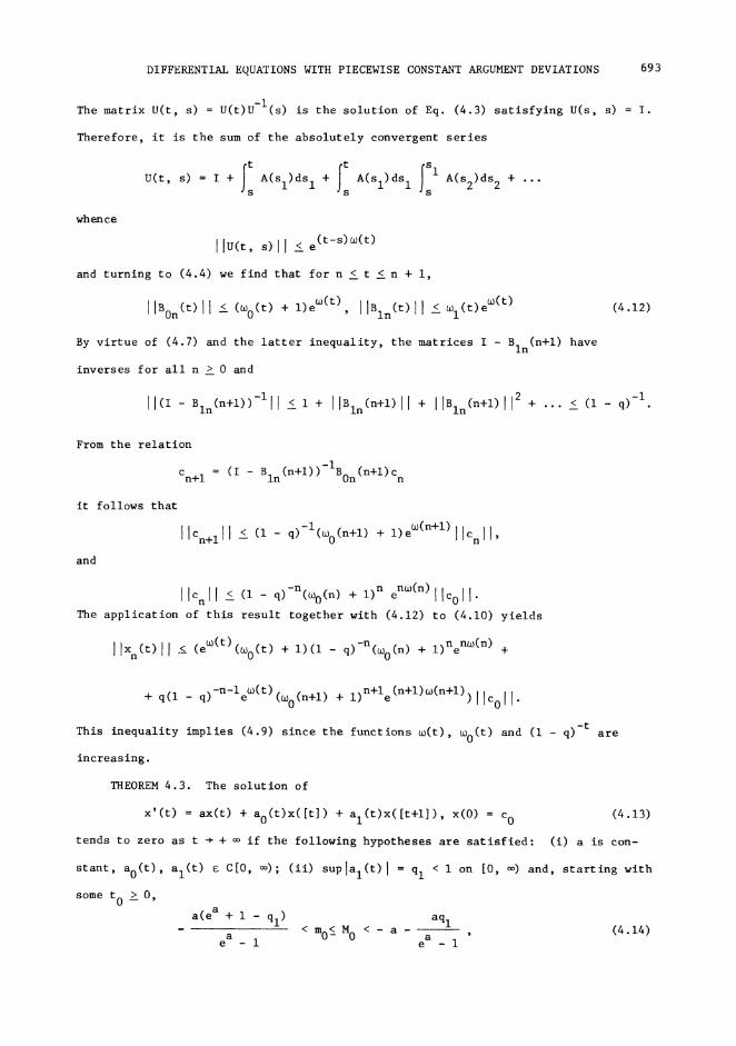
DIFFERENTIAL EQUATIONS WITH PIECEWISE CONSTANT ARGUMENT DEVIATIONS 693
-IThe matrix U(t, s) U(t)U (s) is the solution of Eq. (4.3) satisfying U(s, s) I.
Therefore, it is the sum of the absolutely convergent series
U(t, s) I + A(Sl)dSl + A(Sl)dSli
S S SA(s2)ds2 +
whence
(t-s) (t)flU(t, s) II _< e
and turning to (4.4) we find that for n <_ t _< n + i,
lB0n(t) II _< (0(t) + l)e(t), llBln(t) ll _< el(t)e(t)
(4 12)
By virtue of (4.7) and the latter inequality, the matrices I Bln(n+l) have
inverses for all n > 0 and
II(I Bln(n+l))-lll _< I + lBln(n+l) II + llBln(n+l) II 2 + _< (i q)-l.
From the relation
Cn+I (I Bln(n+l))-IB (n+l)cOn n
it follows that
and
lCn+ll < (i q)-l(000(n+l) + l)e(n+l) llc I]n
lcn If <_ (1 q)-n(0(n) + i)n end(n) ICol I.
The application of this result together with (4.12) to (4.10) yields
llXn(t) ll --< (e0(t) (o(t) + i)(I q)-n(o(n) + i) nen(n)
+ q(l q)-n-le(t) (0 (n+l) + I) n+le (n+l) (n+l)
This inequality implies (4 9) since the functions (t) 0(t) and (I q)-t are
increasing.
THEOREM 4.3. The solution of
x’(t) ax(t) + a0(t)x([t]) + al(t)x([t+l]) x(0) cO (4.13)
tends to zero as t + if the following hypotheses are satisfied: (i) a is con-
stant, a0(t) al(t) E C[O, ); (ii) suplal(t) ql < i on [0, oo) and, starting with
some to 0,
a(ea + i ql aql< m0< M
0< a (4 14)a a
e -i e -i
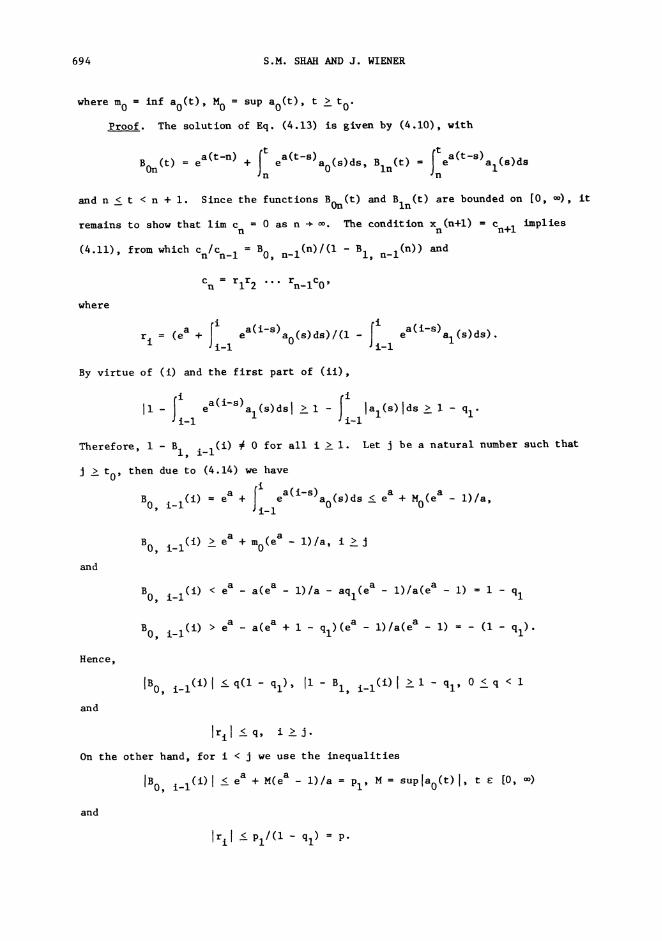
694 S.M. SHAH AND J. WIENER
where m0
inf ao(t), M0
sup ao(t), t >_ toProof. The solution of Eq. (4.13) is given by (4.10), with
t
Bon(t) ea(t-n) + e
a(t-s)
n
t (t-s)a0(s)ds, Bin(t) e
aal(S)ds
and n _< t < n + i. Since the functions Bon(t) and Bin(t) are bounded on [0, ), it
remains to show that lira c 0 as n . The condition x (n+l) c impliesn n n+l
(4.11) from which Cn/Cn_I B0, n_l(n)/(l BI, n-l(n)) and
where
c r.r..., r__.c,n u
ri
(ea + ea(i-s)
i-i
i
ao (s) ds)/(ii-i
ea(i-s) aI (s)ds).
By virtue of (i) and the first part of (il),
a(i-s)Ii e
i-I(s)ds.l > 1aI i-i
lal(s) Ids _> 1 ql"
Therefore, I BI, i_l(i) 0 for all i >_ I. Let j be a natural number such that
j _> to, then due to (4.14) we have
i
BO i-l(1) ea + I ea(i-S)ao(s)ds < ea + MO(ea l)/a,i-I
and
B0, i-i
B0,
(i) _> ea + mo(ea l)/a, i _> j
(1) < ea a(ea l)/a aql(e
a l)/a(ea i) I ql
a( + I- ql)( l)/a( i) (I ql).BO, i-i(i) > e
aea
ea e
a
Hence,
and
{B0, +/-_(i) < q( ql II BI, f_l(f) >_ i ql’ 0 <_ q < i
]r+/-] <_q, i_>j.
On the other hand, for i < j we use the inequalities
ISo, i_Ci) l-< + e- )/ p, suplao()I, [o, )
and
r l< Pl/( 1 ql P-
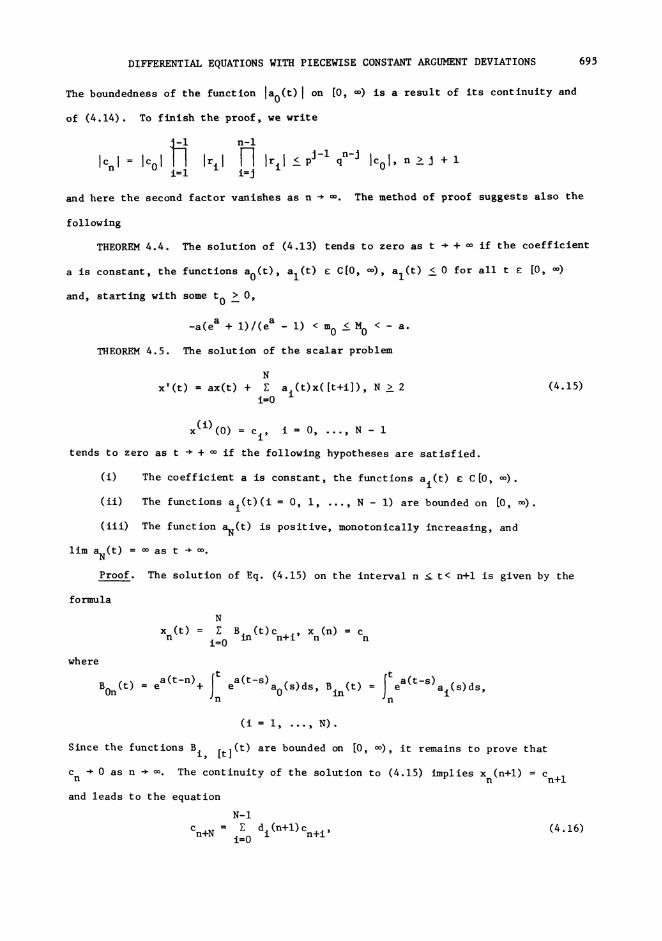
DIFFERENTIAL EQUATIONS WITH PIECEWISE CONSTANT ARGUMENT DEVIATIONS 695
The boundedness of the function [a0(t) on [0, =o) is a result of its continuity and
of (4.14). To finish the proof, we write
Icnl Iol I+/-l ]--[ ]ril < pj-1 qn-j {Col n > j + 1i=l
and here the second factor vanishes as n / m. The method of proof suggests also the
following
THEOREM 4.4. The solution of (4.13) tends to zero as t / + if the coefficient
a is constant, the functions a0(t) al(t) e C[O, ), al(t) <_ 0 for all t e [0, )
and, starting with some tO _> 0,
-a(ea + l)/(ea i) < m0
<_ M0
< a.
THEOREM 4.5. The solution of the scalar problem
Nx’(t) ax(t) + F.
i=0ai(t)x([t+i]) N _> 2 (4.15)
x(i)(0) ci, i-- 0, N- i
tends to zero as t / + if the following hypotheses are satisfied.
(i) The coefficient a is constant, the functions ai(t) E C[0,
(ii) The functions a.(t)(i 0, i, N I) are bounded on [0,1
(iii) The function aN(t) is positive, monotonically increasing, and
lira aN(t) as t / .Proof. The solution of Eq. (4.15) on the interval n t< n+l is given by the
formula
Nx (t) 7. Bin(t)Cn+i,_ Xn(n)_ cn ni=0
where
Bon(t) ca(t-n)+ Jt Itea(t-S)a0(s)ds B (t) ea(t-s)
inn nai(s) ds,
(i i, N).
Since the functions Bi, [t](t) are bounded on [0, =o), it remains to prove that
c 0 as n oo. The continuity of the solution to (4.15) implies x (n+l) cn n n+l
and leads to the equation
N-I
Cn+N Z di(n+l) Cn+i, (4.16)i=O
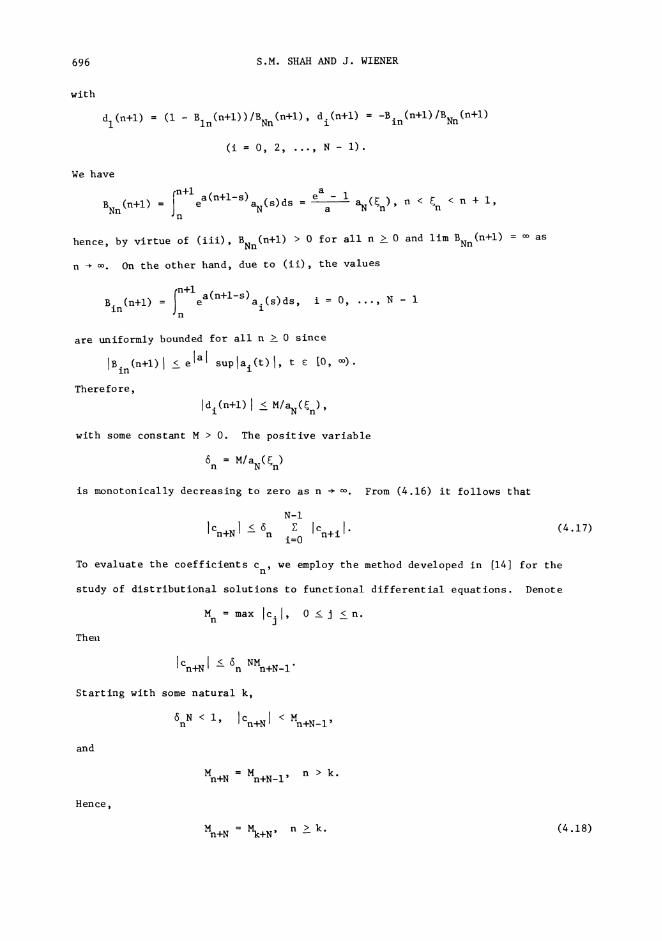
696 S.M. SHAH AND J. WIENER
with
dl(n+l) (i Bln(n+l))/BNn(n+l), di(n+l) -Bin(n+l)/BNn(n+l)
(i 0, 2, N 1).
We have
n+l a (n+l-s)eBNn (n+l) ]n aN(s) ds a
a
aN(n) n < n < n + I,
hence, by virtue of (iii), BNn(n+l) > 0 for all n >_ 0 and lira BNn(n+l) as
n oo. On the other hand, due to (ii), the values
n+l a(n+l-s)Bin (n+l) e
-na.ts)es, u,1
are uniformly bounded for all n >_ 0 since
IBin(n+l) <_ elal suplai(t)I, t [0, o).
Therefore,
Idi (n+l) --< M/aN(n),
with some constant M > 0. The positive variable
6n M/aN(n)
is monotonically decreasing to zero as n oo. From (4.16) it follows that
N-I
ICn+N! < r.n Cn+i
i=0
To evaluate the coefficients c we employ the method developed in [14] for then
study of distributional solutions to functional differential equations. Denote
Mn max cjl, 0 _< j _< n.
Then
Cn+Nl <-- NMn+N_I.n
Starting with some natural k,
N<I, <n Cn+N Mn+N-1
and
Mn+N Mn+N_I, n > k.
Hence,
Mn+N Mk+N, n >_ k.
(4.17)
(4.18)
DIFFERENTIAL EQUATIONS WITH PIECEWISE CONSTANT ARGUMENT DEVIATIONS 697
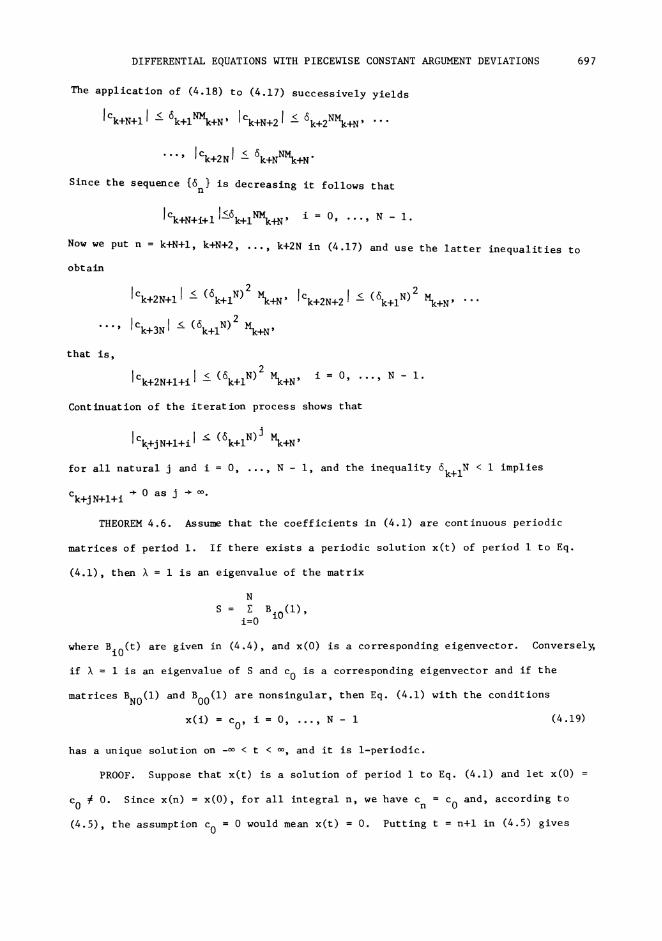
The application of (4.18) to (4.17) successively yields
Ck+N+l I-< 6k+iNMk+N, ;Ck+N+21 --< k+2NMk+N
Ck+2Nl --< 6k+NN+N-Since the sequence {6 is decreasing it follows thatn
ICk+N+i+I I<--6k+IN+N, i O, N i.
Now we put n k+N+l, k+N+2, ..., k+2N in (4.17) and use the latter inequalities to
obtain
ICk+2N+l --< (6k+iN)2 +N’ ICk+2N+21 -< (6k+iN)2 +N’2Ck+BNl <-- (6k+iN) Mk+N,
that is,
Ck+2N+l+il < (6k+IN)2 Mk+N i 0, N I.
Continuation of the iteration process shows that
ICk.+jN+l+i (k+IN)jMk+N,
for all natural j and i 0, N I, and the inequality 6k+IN < i implies
+0 asj /oo.Ck+j N+l+i
THEOREM 4.6. Assume that the coefficients in (4.1) are continuous periodic
matrices of period I. If there exists a periodic solution x(t) of period i to Eq.
(4.1), then % I is an eigenvalue of the matrix
NS Y Bio(1)
i=0
where Bi0(t) are given in (4.4), and x(O) is a corresponding eigenvector. Conversel
if 1 is an eigenvalue of S and co is a corresponding eigenvector and if the
matrices BN0(1) and B00(1) are nonsingular, then Eq. (4.1) with the conditions
x(i) Co, i O, N- 1 (4.19)
has a unique solution on < t < oo, and it is 1-periodic.
PROOF. Suppose that x(t) is a solution of period i to Eq. (4.1) and let x(0)
co # 0. Since x(n) x(O), for all integral n, we have Cn Co and, according to
(4.5), the assumption co 0 would mean x(t) 0. Putting t n+l in (4.5) gives
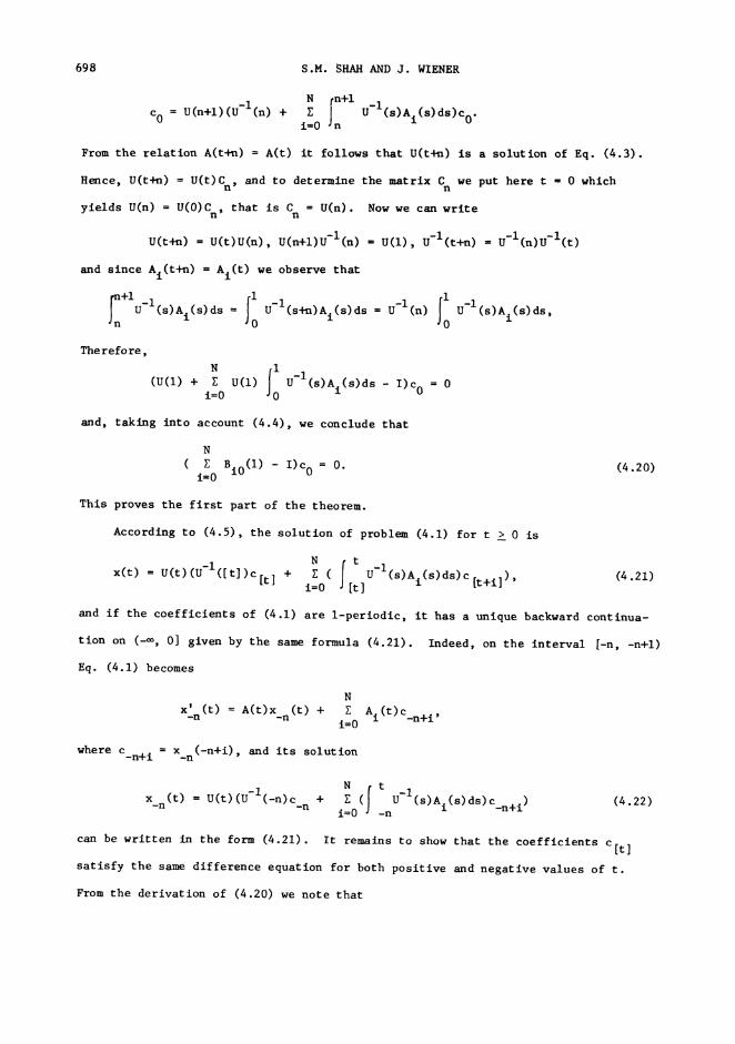
698 S.M. SHAH AND J. WIENER
cOU(n+l)(u-l(n) +
N [n+l7. u-l(s)Ai(s) ds) c0iffi0 -n
From the relation A(t+n) A(t) it follows that U(t+n) is a solution of Eq. (4.3).
Hence, U(t+n) U(t)Cn, and to determine the matrix C we put here t 0 whichn
yields U(n) U(0)C that is C U(n). Now we can writen n
U(t+n) U(t)U(n), U(n+I)U-I (n) U(1), u-l(t+n) u-l(n)u-l(t)and since Ai(t+n) Ai(t) we observe that
U- (s)At(s)ds U-l(s-t)Ai(s)ds u-l(n) U-l(s)i(s)ds0 0
Therefore,N 1
(U(1) + 7. U(1) I u-l(s)Ai(s)ds I)co 0i=0 0
and, taking into account (4.4), we conclude that
NZ Bio(1) I)c
0O.
i=O(4.20)
This proves the first part of the theorem.
According to (4.5), the solution of problem (4.1) for t > 0 is
x(t) U(t)(u-l([t])c[t] +i=O It
U-I(s)Ai(s) ds) c it+i]), (4.21)
and if the coefficients of (4.1) are 1-perlodlc, it has a unique backward continua-
tion on (_oo, 0] given by the same formula (4.21). Indeed, on the interval [-n, -n+l)
Eq. (4.1) becomes
N
X’_n(t) A(t)X_n(t) + 7. Ai‘_(t)c_n+i
i=0
where C_n+i x (-n+i), and its solution-n
x (t) U(t)(u-l(-n)c + 7. u-l(s)Ai(s)ds)c_n+i-n -ni=O -n
(4.22)
can be written in the form (4.21). It remains to show that the coefficients c[tsatisfy the same difference equation for both positive and negative values of t.
From the derivation of (4.20) we note that
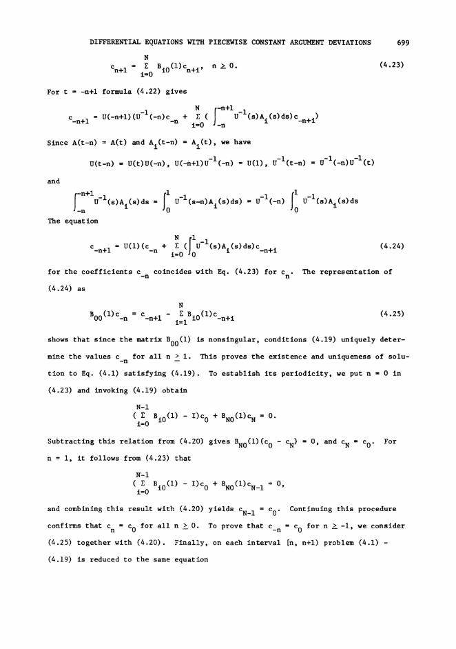
DIFFERENTIAL EQUATIONS WITH PIECEISE CONSTANT ARGUHENT DEVIATIONS 699
NZ Bio(1)Cn+i, n > O.Cn+li=O
(4.23)
For t =-n+l formula (4.22) gives
C-n+l
U(-n/l) (U-1N I-n+l 1
(-n)c + " --nU- (s)Ai(s)ds)c_n+f)-n
i=O
Since A(t-n) A(t) and Ai(t-n) Ai(t), we have
U(t-n) U(t)U(-n), U(-h+l)U-l(-n) U(1), u-l(t-n) u-l(-n)u-l(t)
and
f-n+l -I II -i IIU (s)A. (s) U-1J-n ds (s-n)Ai(s)ds) U (-n) u-l(s)Ai(s)ds0 0
The equat ion
U(1)(c / l l(s)Af(s)ds)c_n/f (4.24)C-n+1 -ni=0
for the coefficients c coincides with Eq. (4.23) for c The representation of-n n
(4.24) as
N
B00(1)C_n C_n+l iZIBi0(1)C_n+i= (4.25)
shows that since the matrix B00(1) is nonsingular, conditions (4.19) uniquely deter-
mine the values c for all n > I. This proves the existence and uniqueness of solu--n
tion to Eq. (4.1) satisfying (4.19). To establish its periodicity, we put n 0 in
(4.23) and invoking (4.19) obtain
N-I7. Bi0(1) l)c
0+ BNO(1)cN 0.
i=0
Subtracting this relation from (4.20) gives BN0(1)(c0 cN) 0, and cN co For
n I, it follows from (4.23) that
N-Ir. Bio(1) l)c
0 + BNO(1)CN_1 O,i=O
and combining this result with (4.20) yields CN_I c0. Continuing this procedure
confirms that Cn co for all n _> O. To prove that C_n co for n _> -I, we consider
(4.25) together with (4.20). Finally, on each interval [n, n+l) problem (4.1)
(4.19) is reduced to the same equation
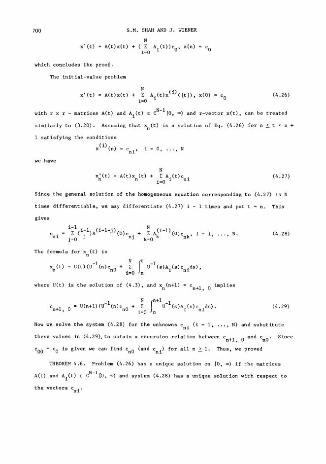
7OO S.M. SHAH AND J. WIENER
Nx’(t) A(t)x(t) + 7 Ai(t))c0, x(n) cn
i=0
which concludes the proof.
The initial-value problem
Nx’(t) A(t)x(t) + 7 A.(t)x(i) (It]), x(O) co (4.26)
i=O
with r x r matrices A(t) and Ai(t) cN-I[o, oo) and r-vector x(t), can be treated
similarly to (3.20). Assuming that x (t) is a solution of Eq. (4.26) for n < t < n +n
i satisfying the conditions
(i)x (n) Cni i 0, N
we have
Nx’(t) A(t)x (t) + 7. Ai(t)c (4 27)n n
i=0ni
Since the general solution of the homogeneous equation corresponding to (4.27) is N
times differentiable, we may differentiate (4.27) i i times and put t n. This
gives
i 1c (i-.l)A(i-l-j)ni
j=0 J
N
(0)Cnj + Z i-l)k=O
(O)Cnk i I, N. (4.28)
The formula for x (t) isn
Xn(t) U(t)(u-l(n)Cn0 + NitY. U-l(s)Ai(s)c ids)ni=0 n
where U(t) is the solution of (4.3), and Xn(n+l) Cn+l, 0 implies
[n+Iu-i (s)c ids). (4.29)Cn+l 0U(n+l) (u-l(n)Cn0 + (s)Ai n
i 0 -n
Now we solve the system (4.28) for the unknowns c (i i, N) and substitutenl
these values in (4.29), to obtain a recursion relation between Cn+l, 0and Cn0. Since
Co0 co is given we can find Cn0 (and Cni for all n _> I. Thus, we proved
THEOREM 4.6. Problem (4.26) has a unique solution on [0, o) if the matrices
cN-1A(t) and A.(t) e [0, oo) and system (4.28) has a unique solution with respect to1
the vectors cni"
DIFFERENTIAL EQUATIONS WITH PIECEWISE CONSTANT ARGUMENT DEVIATIONS 701
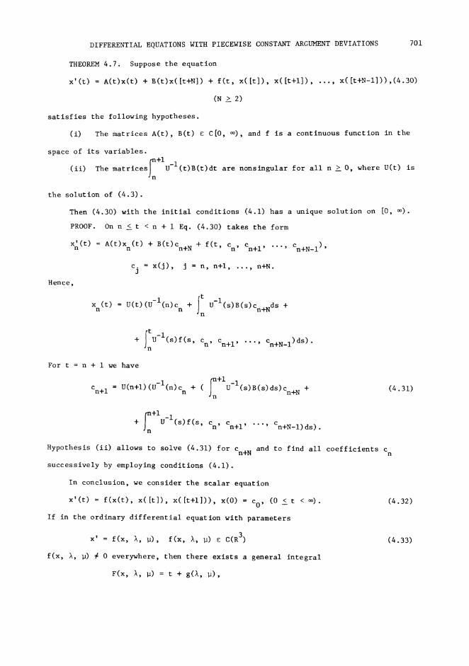
THEOREM 4.7. Suppose the equation
x’(t) A(t)x(t) + B(t)x([t+N]) + f(t, x([t]), x([t+l]), x([t+N-1])),(4.30)
(N -->2)
satisfies the following hypotheses.
(i) The matrices A(t), B(t) e C[0, oo), and f is a continuous function in the
space of its variables.
(ii) The matrices|L+Iu-l(t)B(t)dt are nonsingular for all n >_ 0, where U(t) is
In
the solution of (4.3).
Then (4.30) with the initial conditions (4.1) has a unique solution on [0, oo).
PROOF. On n <_ t < n + I Eq. (4.30) takes the form
x’(t) A(t)x (t) + B(t)c + f(t cn Cn+N_l)n n n+N Cn+l’
Hence,
c. x(j), j n, n+l, n+N.
x (t) U(t)(U-In
tU-I(n)Cn + (s)B(S)Cn+Nds +
n
+ [tu-l(s)f(s, cn, Cn+I, ..., Cn+N_l)dS)."n
For t n + i we have
Cn+I U(n+l) (U-In+l I
(n)Cn + U- (s)B(s)ds)cn+N +n
(4.31)
+ I+Iu-l(s)f(s, cn, Cn+I Cn+N_l) ds).
Hypothesis (ii) allows to solve (4.31) for Cn+N and to find all coefficients cn
successively by employing conditions (4.1).
In conclusion, we consider the scalar equation
x’(t) f(x(t), x([t]), x([t+l])), x(0) Co, (0 <_ t < oo).
If in the ordinary differential equation with parameters
(4.32)
x’ f(x, %, ), f(x, %, ) e C(R3)f(x, %, ) # 0 everywhere, then there exists a general integral
(4.33)
F(x, %, ) t + g(%, ),
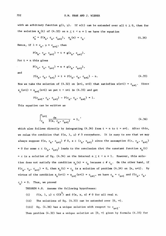
702 S.M. SHAH AND J. WIENER
with an arbitrary function g(%, ). If x(t) can be extended over all t >_ 0, then for
the solution x (t) of (4.32) on n < t < n + I we have the equationn
X’n f(Xn’ Cn’ Cn+I), xn(n) Cn. (4.34)
Hence, if % Cn, Cn+I, then
F(x Cn, t + g(cn’ Cn+l n’ Cn+l
For t n this gives
and
F(c cn
n + g(cn Cn+l)n Cn+l
F(Xn, Cn, cn+l
t + F(Cn, Cn, cn+l n. (4.35)
Now we take the solution of (4.32) on [n+l, n+2) that satisfies x(n+l) Cn+I. Since
Xn(n+l) Xn+l(n+l) we put t n+l in (4.35) and get
F(Cn+I, cn, Cn+I) F(Cn, Cn’ Cn+l I.
This equation can be written as
cn+ldx
Cn f(x, cn, Cn+I)1, (4.36)
which also follows directly by integrating (4.34) from t n to t n+l. After this,
we relax the condition that f(x, , ) 0 everywhere. It is easy to see that we may
always suppose f(x, Cn, Cn+I) # 0, x e (Cn, Cn+l since the assumption f(c, Cn, Cn+l
0 for some c e _(Cn, Cn+I)_ leads to the conclusion that the constant function Xn(t)
c is a solution of Eq. (4.34) on the interval n <_ t < n + i. However, this solu-
tion does not satisfy the condition Xn(n) Cn because c # Cn. On the other hand, if
f(c Cn, Cn+I) 0, then x (t) c is a solution of problem (4.34) on [n, n+l). Byn n n
virtue of the condition x (n+l) xn n+l
(n+l) Cn+l, we have Cn Cn+l and f(Cn, Cn’
c 0. Thus, we provedn
THEOREM 4.8. Assume the following hypotheses:
(i) f(x, , ) e C(R3) and f(x, x, x) 0 for all real x.
(ii) The solutions of Eq. (4.33) can be extended over [0, ).
(iii) Eq. (4.36) has a unique solution with respect to Cn+I.Then problem (4.32) has a unique solution on [0, ) given by formula (4.35) for
DIFFERENTIAL EQUATIONS WITH PIECEWISE CONSTANT ARGUMENT DEVIATIONS 703
t e [n, n+l], where
f(x,dxF(x, , ) .,,^ )
If f(Cn, nCn, cn) 0, then x(t) c is a solution on [n, ) of Eq. (4 32) with
the condition x(n) cn
REFERENCES
i. Shah, S.M. and Wiener, J. Distributional and entire solutions of ordinarydifferential and functional differential equations, Inter. J. Math. & MathSci. 6(2), (1983), 243-270.
2. Cooke, K.L. and Wiener, J. Distributional and analyt ic solutions of funct ionaldifferential equations, J. Math. Anal. and Appl. (to appear).
3. Pelyukh, G.P. and Sharkovskii, A.N. Introduction to the Theory of FunctionalEquations (Russian), Naukova Dumka, Kiev, 1974.
4. Halanay, A. and Wexler, D. Teorla Calitatlvav
a Sistemelor cu Impulsuri, Acad.RSR, Bucuresti, 1968.
5. Myshkis, A.D. On certain problems in the theory of differential equations withdeviating argument, Uspekhl Mat. Nauk 32(2), (1977), 173-202.
6. Busenberg, S. and Cooke, K.L. Models of vertically transmitted diseases withsequential-continuous dynamics, in Nonlinear Phenomena in MathematicalSciences, Lakshmikantham, V. (editor), Academic Press, New York, 1982, 179-187.
7. Kamenskii, G.A. Towards the general theory of equations with deviating argu-ment, DAN SSSR 120(4), (1958), 697-700.
8. Cooke, K.L. and Wiener, J. Retarded differential equations with plecewlseconstant delays, J. Math. Anal. and Appl. (to appear).
9. Wiener, J. Differential equations with piecewise constant delays, in Trends inthe Theor and Practice of Nonlinear Differential Equat.ions Lakshmlkantham, V.(editor), Marcel Dekker, New York, 1983, 547-552.
i0. Wiener, J. Pointwise initial-value problems for functional differential equa-tions, in Proceedings of the International Conference on Differential Equationsat The University of Alabama in Birmingham, March 21-26, 1983, Knowles, Ian andLewis, Rogers (editors), to appear.
ii. Hale, J.K. Theor of Functional Differential Equat.ions Springer-Verlag, NewYork, 1977.
12. Shah, S.M. On real continuous solutions of algebraic difference equations,Bull. Amer. Math. Soc. 53(1947), 548-558.
13. Shah, S.M. On real continuous solutions of algebraic difference equations, II,Proc. Nat. Inst. Sci. India 16(1950), 11-17.
14. Wiener, J. Generalized-function solutions of linear systems, J. Differ. Equat.38(2), (1980), 301-315.