Advanced Econometrics - HEC Lausanne Christophe Hurlin€¦ · 2. What is an Estimator? Question: What constitues a good estimator? 1 The search for good estimators constitutes much

Chapter 1: Estimation TheoryAdvanced Econometrics - HEC Lausanne

Christophe Hurlin

University of Orléans

November 20, 2013

Christophe Hurlin (University of Orléans) Advanced Econometrics - HEC Lausanne November 20, 2013 1 / 147

Section 1

Introduction


1. Introduction

Estimation problem

Let us consider a continuous random variable Y characterized by amarginal probability density function fY (y ; θ) for y 2 R and θ 2 Θ.The parameter θ is unknown.

Let fY1, ..,YNg a random sample of i .i .d . random variables that havethe same distribution as Y .

We have one realisation fy1, .., yNg of this sample.

How to estimate the parameter θ?


1. Introduction

Remarks

1 The estimation problem can be extended to the case of aneconometric model. In this case we consider two variables Y and Xand a conditional pdf fY jX=x (y ; θ) that depends on a parameter or avector of unknown parameters θ.

2 In this chapter, we dont derive the estimators (for the estimationmethods, see next chapters). We admit that we have an estimator bθfor θ whatever the estimation method used and we study its nitesample and large sample properties.


1. Introduction

Notations: In this course, I will (try to...) follow some conventions ofnotation.

Y random variabley realisationfY (y) probability density or mass functionFY (y) cumulative distribution functionPr () probabilityy vectorY matrix

Problem: this system of notations does not allow to discriminate betweena vector (matrix) of random elements and a vector (matrix) ofnon-stochastic elements (realisation).

Abadir and Magnus (2002), Notation in econometrics: a proposal for astandard, Econometrics Journal.


1. Introduction

The outline of this chapter is the following:

Section 2: What is an estimator?

Section 3: Finite sample properties

Section 4: Large sample properties

Subsection 4.1: Almost sure convergence

Subsection 4.2: Convergence in probability

Subsection 4.3: Convergence in mean square

Subsection 4.4: Convergence in distribution

Subsection 4.5: Asymptotic distributions


Section 2

What is an Estimator?


2. What is an Estimator?

Objectives

1 Dene the concept of estimator.

2 Dene the concept of estimate.

3 Sampling distribution.

4 Discussion about the notion of "good "estimator.



Denition (Point estimator)

A point estimator is any function T (Y1,Y2, ..,YN ) of a sample. Anystatistic is a point estimator.


What is an estimator?

Example (Sample mean)

Assume that Y1,Y2, ..,YN are i .i .d . Nm, σ2

random variables. The

sample mean (or average)

Y N =1N

N

∑i=1Yi

is a point estimator (or an estimator) of m.



Example (Sample variance)

Assume that Y1,Y2, ..,YN are i .i .d . Nm, σ2


sample variance

S2N =1

N 1N

∑i=1

Yi Y N

2is a point estimator (or an estimator) of σ2.





Fact

An estimator bθ is a random variable.

Consequence: bθ has a (marginal or conditional) probability distribution.This sampling distribution is caracterized by a probability densityfunction (pdf) fbθ (u)



Denition (Sampling Distribution)

The probability distribution of an estimator (or a statistic) is called thesampling distribution.



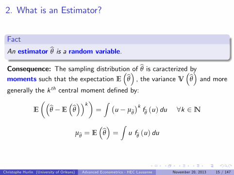
Fact

An estimator bθ is a random variable.

Consequence: The sampling distribution of bθ is caracterized bymoments such that the expectation E

bθ , the variance Vbθ and more

generally the k th central moment dened by:

E

bθ Ebθk = Z

u µbθk fbθ (u) du 8k 2 N

µbθ = Ebθ = Z

u fbθ (u) du



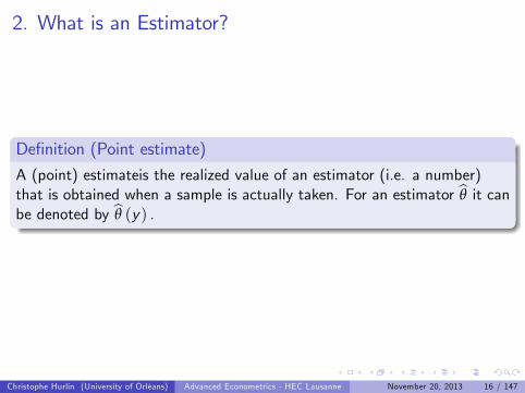
Denition (Point estimate)

A (point) estimateis the realized value of an estimator (i.e. a number)that is obtained when a sample is actually taken. For an estimator bθ it canbe denoted by bθ (y) .



Example (Point estimate)For instance yN is an estimate of m.

yN =1N

N

∑i=1yi

If N = 3 and fy1, y2, y3g = f3,1, 2g then yN = 1.333.If N = 3 and fy1, y2, y3g = f4,8, 1g then yN = 1.etc..



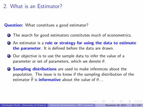
Question: What constitues a good estimator?

1 The search for good estimators constitutes much of econometrics.

2 An estimator is a rule or strategy for using the data to estimatethe parameter. It is dened before the data are drawn.

3 Our objective is to use the sample data to infer the value of aparameter or set of parameters, which we denote θ.

4 Sampling distributions are used to make inferences about thepopulation. The issue is to know if the sampling distribution of theestimator bθ is informative about the value of θ....



Question (contd): What constitues a good estimator?

1 Obviously, some estimators are better than others.

1 To take a simple example, your intuition should convince you that thesample mean would be a better estimator of the population mean thanthe sample minimum; the minimum is almost certain to underestimatethe mean.

2 Nonetheless, the minimum is not entirely without virtue; it is easy tocompute, which is occasionally a relevant criterion.

2 The idea is to study the properties of the sampling distributionand especially its moments such as E

bθ (for the bias), Vbθ (for

the precision), etc..



Question (contd): What constitues a good estimator?

Estimators are compared on the basis of a variety of attributes.

1 Finite sample properties (or nite sample distribution) of estimatorsare those attributes that can be compared regardless of the samplesize (SECTION 3).

2 Some estimation problems involve characteristics that are unknown innite samples. In these cases, estimators are compared on the basison their large sample, or asymptotic properties (SECTION 4).



Key Concepts Section 2

1 Point estimator2 Point estimate3 Sampling distribution


Section 3

Finite Sample Properties


3. Finite Sample Properties

Objectives

1 Dene the concept of nite sample distribution.

2 Finite sample properties => What is a good estimator?

3 Unbiased estimator.

4 Comparison of two unbiased estimators.

5 FDCR or Cramer Rao bound.

6 Best Linear Unbiased Estimator (BLUE).



Denition (Finite sample properties and nite sample distribution)

The nite sample properties of an estimator bθ correspond to the propertiesof its nite sample distribution (or exact distribution) dened for anysample size N 2 N.



Two cases:

1 In some particular cases, the nite sample distribution of theestimator is known. It corresponds to the distribution of the randomvariable bθ for any sample size N.

2 In most of cases, the nite sample distribution is unknown, but wecan study some specic moments (mean, variance, etc..) of thisdistribution (nite sample properties).



Example (Sample mean and nite sample distribution)

Assume that Y1,Y2, ..,YN are N .i .d .m, σ2


estimator bm = Y N (sample mean) has also a normal distribution:bm = 1

N

N

∑i=1Yi N

m,

σ2

N

8N 2 N

Consequence: the nite sample distribution of bm for any N 2 N is fullycharacterized by m and σ2 (parameters that can be estimated). Example:if N = 3, then bm N

m, σ2/3, if N = 10, then bm N

m, σ2/10,

etc..



Proof: The sum of independent normal variables has a normal distributionwith:

E (bm) = 1N

N

∑i=1

E (Yi ) =NmN= m

V (bm) = V

1N

N

∑i=1Yi

!=

1N2

N

∑i=1

V (Yi ) =Nσ2

N2=

σ2

N

since the variables Yi are

independent (then cov (Yi ,Yj ) = 0)identically distributed (then E (Yi ) = m and V (Yi ) = σ2,8i 2 [1, ..,N ]).



Remarks

1 Except in very particular cases (normally distributed samples), theexact distribution of the estimator is very di¢ cult to calculate.

2 Sometimes, it is possible to derive the exact distribution of atransformed variable g

bθ , where g (.) is a continuous function.



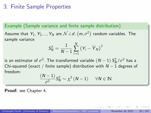
Example (Sample variance and nite sample distribution)



sample variance

S2N =1

N 1N

∑i=1

Yi Y N

2is an estimator of σ2. The transformed variable (N 1) S2N/σ2 has aChi-squared (exact / nite sample) distribution with N 1 degrees offreedom:

(N 1)σ2

S2N χ2 (N 1) 8N 2 N

Proof: see Chapter 4.



FactIn most of cases, it is impossible to derive the exact / nite sampledistribution for the estimator (or a transformed variable).

Two reasons:

1 In some cases, the exact distribution of Y1,Y2..YN is known, but thefunction T (.) is too complicated to derive the distribution of bθ :

bθ = T (Y1, ..YN ) ??? 8N 2 N

2 In most of cases, the distribution of the sample variables Y1,Y2..YN isunknown... bθ = T (Y1, ..YN ) ??? 8N 2 N



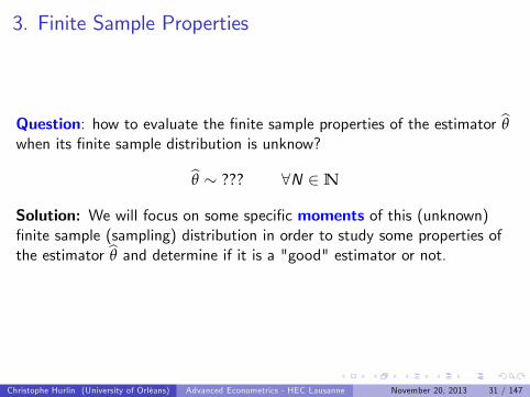
Question: how to evaluate the nite sample properties of the estimator bθwhen its nite sample distribution is unknow?

bθ ??? 8N 2 N

Solution: We will focus on some specic moments of this (unknown)nite sample (sampling) distribution in order to study some properties ofthe estimator bθ and determine if it is a "good" estimator or not.



Denition (Unbiased estimator)

An estimator bθ of a parameter θ is unbiased if the mean of its samplingdistribution is θ:

Ebθ = θ

orEbθ θ

= Bias

bθ θ= 0

implies that bθ is unbiased. If θ is a vector of parameters, then theestimator is unbiased if the expected value of every element of bθ equalsthe corresponding element of θ.



Source: Greene (2007), Econometrics



Example (Bernouilli distribution)Let Y1,Y2, ..,YN be a random sampling from a Bernoulli distribution witha success probability p. An unbiased estimator of p is

bp = 1N

N

∑i=1Yi

Proof: Since the Yi are i .i .d . with E (Yi ) = p, then we have:

E (bp) = 1N

N

∑i=1

E (Yi ) =pNN= p



Example (Uniform distribution)Let Y1,Y2, ..,YN be a random sampling from a uniform distribution U[0,θ].An unbiased estimator of θ is

bθ = 2N

N

∑i=1Yi

Proof: Since the Yi are i .i .d . with E (Yi ) = (θ + 0) /2 = θ/2, then wehave:

Ebθ = E

2N

N

∑i=1Yi

!=2N

N

∑i=1

E (Yi ) =2N Nθ

2= θ



Example (Multiple linear regression model)Consider the model

y = Xβ+ µ

where y 2 RN , X 2 MNK is a nonrandom matrix, β 2 RK is a vector ofparameters, E (µ) = 0N1 and V (µ) = σ2IN . The OLS estimator

bβ = X>X1 X>yis an unbiased estimator of β.



Proof: Since y = Xβ+ µ, X 2 MNK is a nonrandom matrix andE (µ) = 0, we have

E (y) = Xβ

As a consequence:

Ebβ =

X>X

1X>E (y)

=X>X

1X>Xβ

= β

The estimator bβ is unbiased.



Remark:

Even it is not relevant in the section devoted to the nite sampleproperties of estimators, we can introduce here the notion ofasymptotically unbiased estimator (which can be considered as a largesample property..).

Here we assume that the estimator bθ = bθN depends on the samplesize N.



Denition (Asymptotically unbiased estimator)

The sequence of estimators bθN (with N 2 N) is asymptotically unbiased if

limN!∞

EbθN = θ



Example (Sample variance)



uncorrected sample variance dened by

eS2N = 1N

N

∑i=1

Yi Y N

2is a biased estimator of σ2 but is asymptotically unbiased.



Proof: We known that:

S2N =1

N 1N

∑i=1

Yi Y N

2(N 1)

σ2S2N χ2 (N 1) 8N 2 N

Since, we have a relationship between S2N and eS2N , such that:eS2N = 1

N

N

∑i=1

Yi Y N

2=

N 1N

S2N

then we get:Nσ2eS2N χ2 (N 1) 8N 2 N



Proof (contd):

Nσ2eS2N χ2 (N 1) 8N 2 N

Reminder: If X χ2 (v) , then E (X ) = v and V (X ) = 2v . By denition:

E

Nσ2eS2N = N 1

or equivalently:

EeS2N = N 1N

σ2 6= σ2

So, eS2N = (1/N)∑Ni=1

Yi Y N

2is a biased estimator of σ2.



Proof (contd): But eS2N = (1/N)∑Ni=1

Yi Y N

2is asymptotically

unbiased since:

limN!∞

EeS2N = lim

N!∞

N 1N

σ2 = σ2

Remark: Even in a more general framework (non-normal), the samplevariance (with a correction for small sample) is an unbiased estimator of σ2

S2N = (N 1)1| z correction for small sample

N

∑i=1

Yi Y N

2ES2N= σ2



Unbiasedness is interesting per se but not so much!

1 The absence of bias is not a su¢ cient criterion to discriminate amongcompetitive estimators.

2 It may exist many unbiased estimators for the same parameter(vector) of interest.



Example (Estimators)

Assume that Y1,Y2, ..,YN are i .i .d . with E (Yi ) = m, the statistics

bm1 = 1N

N

∑i=1Yi

bm2 = Y1are unbiased estimators of m.



Proof: Since the Yi are i .i .d . with E (Yi ) = m, then we have:

E (bm1) = 1N

N

∑i=1

E (Yi ) =NmN= m

E (bm2) = E (Y1) = m

Both estimators bm1 and bm2 of the parameter m are unbiased.



How to compare two unbiased estimators?

When two (or more) estimators are unbiased, the best one is the moreprecise,.i.e. the estimator with the minimum variance.

Comparing two (or more) unbiased estimates becomes equivalent tocomparing their variance-covariance matrices.



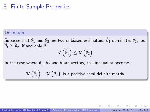
Denition

Suppose that bθ1 and bθ2 are two unbiased estimators. bθ1 dominates bθ2, i.e.bθ1 bθ2, if and only ifVbθ1 V

bθ2In the case where bθ1, bθ2 and θ are vectors, this inequality becomes:

Vbθ2V

bθ1 is a positive semi denite matrix



0 0.5 1 1.5 2 2.5 3 3.5 40

0.1

0.2

0.3

0.4

0.5

0.6

0.7

0.8

θ

Estimator 1Estimator 2



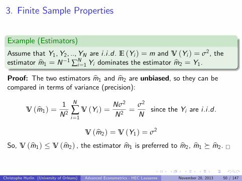
Example (Estimators)

Assume that Y1,Y2, ..,YN are i .i .d . E (Yi ) = m and V (Yi ) = σ2, theestimator bm1 = N1 ∑N

i=1 Yi dominates the estimator bm2 = Y1.Proof: The two estimators bm1 and bm2 are unbiased, so they can becompared in terms of variance (precision):

V (bm1) = 1N2

N

∑i=1

V (Yi ) =Nσ2

N2=

σ2

Nsince the Yi are i .i .d .

V (bm2) = V (Y1) = σ2

So, V (bm1) V (bm2) , the estimator bm1 is preferred to bm2, bm1 bm2. Christophe Hurlin (University of Orléans) Advanced Econometrics - HEC Lausanne November 20, 2013 50 / 147


Question: is there a bound for the variance of the unbiased estimators?



Denition (Cramer-Rao or FDCR bound)

Let X1, ..,XN be an i .i .d . sample with pdf fX (θ; x). Let bθ be an unbiasedestimator of θ; i.e., Eθ(bθ) = θ. If fX (θ; x) is regular then

Vθ

bθ I1N (θ0) = FDCR or Cramer-Rao bound

where IN (θ0) denotes the Fisher information number for the sampleevaluated at the true value θ0. If θ is a vector then this inequality meansthat Vθ

bθI1N (θ0) is positive semi-denite.

FDCR: Frechet - Darnois - Cramer and RaoRemark: we will dene the Fisher information matrix (or number) inChapter 2 (Maximum Likelihood Estimation).



Denition (E¢ ciency)

An estimator is e¢ cient if its variance attains the FDCR (Frechet -Darnois - Cramer - Rao) or Cramer-Rao bound:

Vθ

bθ = I1N (θ0)

where IN (θ0) denotes the Fisher information matrix associated to thesample evaluated at the true value θ0.



Finally, note that in some cases we further restrict the set of estimators tolinear functions of the data.

Denition (Estimator BLUE)An estimator is the minimum variance linear unbiased estimator or bestlinear unbiased estimator (BLUE) if it is a linear function of the data andhas minimum variance among linear unbiased estimators



Remark: the term "linear" means that the estimator bθ is a linear functionof the data Yi : bθj = N

∑i=1

ωijYi




1 Finite sample distribution2 Finite sample properties3 Bias and unbiased estimator4 Comparison of unbiased estimators5 Cramer-Rao or FDCR bound6 E¢ cient estimator7 Linear estimator8 Estimateur BLUE


Section 4

Asymptotic Properties


4. Asymptotic Properties

Problem:

1 Let us consider an i .i .d . sample Y1,Y2..,YN , where Y has a pdffY (y ; θ) and θ is an unknown parameter.

2 We assume that fY (y ; θ) is also unknown (we do not know thedistribution of Yi ).

3 We consider an estimator bθ (also denoted bθN to show that it dependson N) such that bθ = T (Y1,Y2, ..,YN ) bθN

4 The nite sample distribution of bθN is unknown....bθN ??? 8N 2 N



Question: what is the behavior of the random variable bθN when thesample size N tends to innity?

Denition (Asymptotic theory)Asymptotic or large sample theory consists in the study of thedistribution of the estimator when the sample size is su¢ ciently large.

The asymptotic theory is fundamentally based on the notion ofconvergence...



We are mainly concerned with four modes of convergence:

1 Almost sure convergence

2 Convergence in probability

3 Convergence in quadratic mean

4 Convergence in distribution.









Section 4


4.1. Almost Sure Convergence


4. Asymptotic Properties4.1. Almost sur convergence

Denition (Almost sure convergence)Let XN be a sequence random variable indexed by the sample size. XNconverges almost surely (or with probability 1 or strongly) to a constantc , if, for every ε > 0,

Pr limN!∞

XN c < ε

= 1

or equivalently if:

PrlimN!∞

XN = c= 1

It is writtenXN

a.s .! c



Comments

1 The almost sure convergence means that the values of XN approachthe value c , in the sense (see almost surely) that events for which XNdoes not converge to c have probability 0.

2 In another words, it means that when N tends to innity, the randomvariable Xn tends to a degenerate random variable (a randomvariable which only takes a single value c) with a pdf equal to aprobability mass function.



0 0.5 1 1.5 2 2.5 3 3.5 40

0.2

0.4

0.6

0.8

1

1.2

c=2



Denition (Strong consistency)

A point estimator bθN of θ is strongly consistent if:

bθN a.s .! θ



Comments When N ! ∞, the estimator tends to a degenerate randomvariable that takes a single value equal to θ.

The crème de la crème (best of the best) of the estimators....
















Section 4


4.2. Convergence in Probability


4. Asymptotic Properties4.2. Convergence in probability

Denition (Convergence in probability)Let XN be a sequence random variable indexed by the sample size. XNconverges in probability to a constant c , if, for any ε > 0,

limN!∞

Pr (jXN c j > ε) = 0

It is writtenXN

p! c or plim XN = c



XNp! c if lim

N!∞Pr (jXN c j > ε) = 0

0 0.5 1 1.5 2 2.5 3 3.5 40

0.5

1

1.5

2

2.5

3

3.5

4

4.5

c=2

cε c+ε

This area tends to 0



XNp! c if lim

N!∞Pr (jXN c j > ε) = 0 for a very small ε...

0 0.5 1 1.5 2 2.5 3 3.5 40

50

100

150

200

250

300

350

400

c=2



Comments

1 The general idea is the same than for the a.s. convergence: XN tendsto a degenerate random variable (even if it is not exactly the case)equal to c ..

2 But when XN is very likely to be close to c for large N, what aboutthe location of the remaining small probability mass which is not closeto c?...

3 Convergence in probability allows more erratic behavior in theconverging sequence than almost sure convergence.



Remark The notationXN

p! X

where X is a random element (scalar, vector, matrix) means that thevariable XN X converges to c = 0.

XN Xp! 0



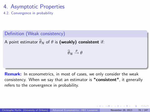
Denition (Weak consistency)

A point estimator bθN of θ is (weakly) consistent if:

bθN p! θ

Remark: In econometrics, in most of cases, we only consider the weakconsistency. When we say that an estimator is "consistent", it generallyrefers to the convergence in probability.



Lemma (Convergence in probability)Let XN be a sequence random variable indexed by the sample size and c aconstant. If

limN!∞

E (XN ) = c

limN!∞

V (XN ) = 0

Then, XN converges in probability to c as N ! ∞ :

XNp! c



Example (Consistent estimator)

Assume that Y1,Y2, ..,YN are i .i .d . with E (Yi ) = m and V (Yi ) = σ2,where σ2 is known and m is unknow. The estimator bm, dened by,

bm = 1N

N

∑i=1Yi

is a consistenty estimator of m.



Proof: Since Y1,Y2, ..,YN are i .i .d . with E (Yi ) = m and V (Yi ) = σ2,we have :

E (bm) = 1N

N

∑i=1

E (Yi ) = m

limN!∞

V (bm) = limN!∞

1N2

N

∑i=1

V (Yi ) = limN!∞

σ2

N= 0

The estimator bm is (weakly) consistent:

bm p! m



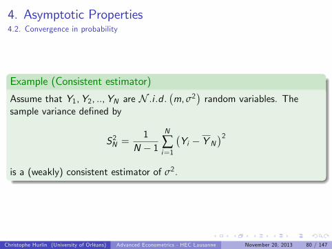
Example (Consistent estimator)



sample variance dened by

S2N =1

N 1N

∑i=1

Yi Y N

2is a (weakly) consistent estimator of σ2.


3. Finite Sample Properties4.2. Convergence in probability

Proof: We known that for normal sample:

(N 1)σ2

S2N χ2 (N 1) 8N 2 N

E

(N 1)

σ2S2N

= N 1 V

(N 1)

σ2S2N

= 2 (N 1)

We get immediately:ES2N= σ2

limN!∞

VS2N= lim

N!∞

2σ4

N 1

= 0

The estimator S2N is (weakly) consistent : S2N

p! σ2.



Lemma (Chain of implication)The almost sure convergence implies the convergence in probability:

a.s .! =) p!

where the symbol "=) " means implies". The converse is not true



Comments

1 One of the main applications of the convergence in probability andthe almost sure convergence is the law of large numbers.

2 The law of large numbers tells you that the sample mean converges inprobability (weak law of large numbers) or almost surely (stronglaw of large numbers) to the population mean:

XN =1N

N

∑i=1Xi !

N!∞E (Xi )



Theorem (Weak law of large numbers, Khinchine)

If fXig , for i = 1, ..,N is a sequence of independently and identicallydistributed (i.i.d.) random variables with nite mean E (Xi ) = µ (<∞),then the sample mean XN converges in probability to µ:

XN =1N

N

∑i=1Xi

p! E (Xi ) = µ



Theorem (Strong law of large numbers, Kolmogorov)

If fXig , for i = 1, ..,N is a sequence of independently and identicallydistributed (i.i.d.) random variables such that E (Xi ) = µ (< ∞) andE (jXi j) < ∞, then the sample mean XN converges almost surely to µ:

XN =1N

N

∑i=1Xi

a.s .! E (Xi ) = µ



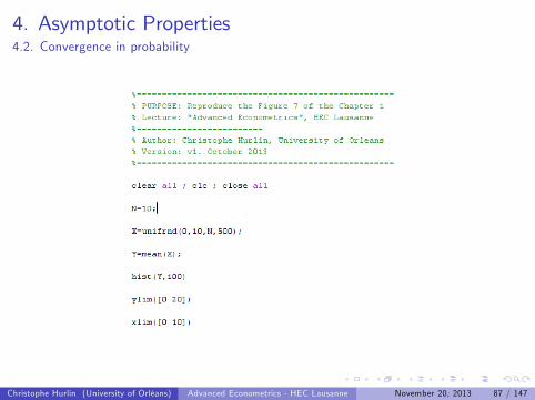
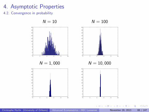
Illustration:

1 Let us consider a random variable Xi U[0,10] and draw an i .i .dsample fxigNi=1

2 Compute the sample mean xN = N1 ∑Ni=1 xi .

3 Repeat this procedure 500 times. We get 500 realisations of thesample mean xN .

4 Build an histogram of these 500 realisations.





N = 10 N = 100

0 2 4 6 8 100

2

4

6

8

10

12

14

16

18

20

0 2 4 6 8 100

2

4

6

8

10

12

14

16

18

20

N = 1, 000 N = 10, 000

0 2 4 6 8 100

2

4

6

8

10

12

14

16

18

20

0 2 4 6 8 100

2

4

6

8

10

12

14

16

18

20



An animation is worth 1,000,000 words...

Click me!



Proof: There are many proofs of the law of large numbers. Most of themuse the additional assumption of nite variance V (Xi ) = σ2 and theChebyshevs inequality.

Theorem (Chebyshevs inequality)Let X be a random variable with nite expected value µ and nitenon-zero variance σ2. Then for any real number k > 0,

Pr (jX µj kσ) 1k2



Proof (contd): Under the assumpition of i .i .d .µ, σ2

, we have that:

EXN= µ V

XN=

σ2

N

Given the Chebyshevs inequality, we get for k > 0:

PrXN µ

k σpN

1k2

Let us dene ε > 0 such that

ε =kσpN() k =

εpN

σ

Then we get for any ε > 0:

PrXN µ

ε σ2

ε2N



Proof (contd): for any ε > 0:

PrXN µ

ε σ2

ε2N

So, when N ! ∞ this probability is necessarily equal to 0 (since 0means = 0)

PrlimN!∞

XN µ ε

= 0 8ε > 0

Since PrXN µ

< ε= 1 P

XN µ ε

, we have:

PrlimN!∞

XN µ < ε

= 1 8ε > 0

XNa.s .! µ (SLLN) =) XN

p! µ (WLLN)



Remarks

1 These two theorems consider a sequence of independently andidentically distributed (i.i.d.) random variables (as a consequencewith the same mean E (Xi ) = µ, 8i = 1, ..,N.

2 There are alternative versions of the law of large numbers forindependent random variables not identically (heterogeneously)distributed with E (Xi ) = µi (cf. Greene, 2007).

1 Chebychevs Weak Law of Large Numbers.

2 Markovs Strong Law of Large Numbers.



Theorem (Slutskys theorem)

Let XN and YN be two sequences of random variables where XNp! X and

YNp! c, where c 6= 0, then:

XN + YNp! X + c

XNYNp! cX

XNYN

p! Xc



Remark: This also holds for sequences of random matrices. The laststatement reads: if XN

p! X and YNp! Ω then

Y1N XNp! Ω1X

provided that Ω1 exists.



ExampleLet us consider the multiple linear regression model

yi = x>i β+ µi

where xi = (xi1..xiK )> is K 1 vector of random variables,

β = (β1...βK )> is K 1 vector of parmeters, and where the error term µi

satises E (µi ) = 0 and E (µi j xij ) = 0 8j = 1, ..K . Question: show thatthe OLS estimator dened by

bβ = N

∑i=1xix>i

!1 N

∑i=1xiyi

!

is a consistent estimator of β.



Proof: let us rewritte the OLS estimator as:

bβ =

N

∑i=1xix>i

!1 N

∑i=1xiyi

!

=

N

∑i=1xix>i

!1 N

∑i=1xix>i β+ µi

!

=

N

∑i=1xix>i

!1 N

∑i=1xix>i

!β+

N

∑i=1xix>i

!1 N

∑i=1xiµi

!

= β+

N

∑i=1xix>i

!1 N

∑i=1xiµi

!



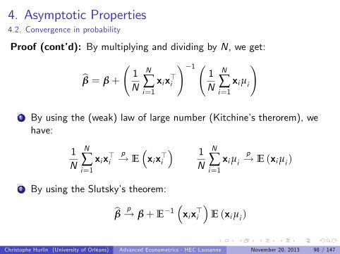
Proof (contd): By multiplying and dividing by N, we get:

bβ = β+

1N

N

∑i=1xix>i

!1 1N

N

∑i=1xiµi

!

1 By using the (weak) law of large number (Kitchines therorem), wehave:

1N

N

∑i=1xix>i

p! Exix>i

1N

N

∑i=1xiµi

p! E (xiµi )

2 By using the Slutskys theorem:

bβ p! β+E1xix>i

E (xiµi )



Reminder: If X and Y are two random variables, then

E (X jY ) = 0 =) E (X Y ) = 0

The reverse is not true.

E (X jY ) = 0 =)(cov (X ,Y ) = E (XY ) E (X )E (Y ) = 0

E (X ) = 0

E (X jY ) = 0 =) E (XY ) = 0



Proof (contd): bβ p! β+E1xix>i

E (xiµi )

SinceE (µi j xij ) = 0 8j = 1, ..K ) E (µixi ) = 0K1

We have bβ p! β

The OLS estimator bβ is (weakly) consistent.
















Section 4


4.3. Convergence in Mean Square


4. Asymptotic Properties4.3. Convergence in mean square

Denition (Convergence in mean square)

Let fXig for i = 1, ..,N be a sequence of real-valued random variables

such that EjXN j2

< ∞. XN converges in mean square to a constant c ,

if:limN!∞

EjXN c j2

= 0

It is writtenXN

m.s .! c


4. Asymptotic Properties4.3. Convergence in mean square

Remark: It is the less usefull notion of convergence.. except for thedemonstrations of the convergence in probability.

Lemma (Chain of implication)The convergence in mean square implies the convergence in probability:

m.s .! =) p!

where the symbol "=) " means implies". The converse is not true.







4 Convergence in distribution







4 Convergence in distribution


Section 4


4.4. Convergence in Distribution


4. Asymptotic Properties4.4. Convergence in distribution

Denition (Convergence in distribution)Let XN be a sequence random variable indexed by the sample size with acdf FN (.). XN converges in distribution to a random variable X withcdf F (.) if

limN!∞

FN (x) = F (x) 8x

It is written:XN

d! X



Comment: In general, we have:

XN|zrandom var.

d! X|zrandom var.

XN|zrandom var.

p! c|zconstant

In the case, where

XN|zrandom var.

p! X|zrandom var.

it means XN X| z random var.

p! 0|zconstant



Lemma (Chain of implication)The convergence in probability implies the convergence in distribution:

p! =) d!

where the symbol "=) " means implies". The converse is not true.



Denition (Asymptotic distribution)

If XN converges in distribution to X , where FN (.) is the cdf of XN , thenF (.) is the cdf of the limiting or asymptotic distribution of XN .



Consequence: Generally, we denote:

XN|zrandom var.

d! L|zasy. distribution

It means XN converges in distribution to a random variable X that has adsitribution L.Example

XNd! N (0, 1)

means that XN converges to a random variable X normally distributed orthat XN has an asymptotic standard normal distribution.



Denition (Asymptotic mean and variance)The asymptotic mean and variance of a random variable XN are themean and variance of the asymptotic or limiting distribution, assumingthat the limiting distribution and its moments exist. These moments aredenoted by

Easy (XN ) Vasy (XN )



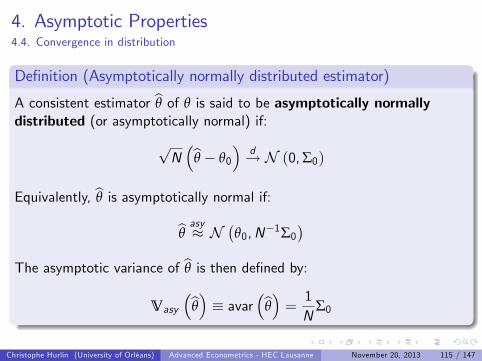
Denition (Asymptotically normally distributed estimator)

A consistent estimator bθ of θ is said to be asymptotically normallydistributed (or asymptotically normal) if:

pNbθ θ0

d! N (0,Σ0)

Equivalently, bθ is asymptotically normal if:bθ asy N

θ0,N1Σ0

The asymptotic variance of bθ is then dened by:

Vasy

bθ avarbθ = 1N

Σ0


Section 4


4.5. Asymptotic Distributions


4. Asymptotic Properties4.5. Asymptotic distributions

Lets go back to our estimation problem

We consider a (strongly) consistent estimator bθN of the trueparameter θ0. bθN a.s .! θ0 =) bθN p! θ0

This estimator has a degenerated asymptotic distribution(point-mass distribution), since when N ! ∞,

limN!∞

fbθN (x) = f (x)where fbθN (.) is the pdf of bθN and f (x) is dened by:

f (x) =10

if x = θ00 otherwise



Conclusion: one needs more than consistency to do inference (testsabout the true value of θ, etc.).

Solution: we will transform the estimator bθN to get a transformedvariable that has a non degenerated asymptotic distribution in order toderive the the asymptotic distribution.

It is the general idea of the Central Limit Theorem for a particularestimator: the sample mean...



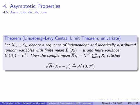
Theorem (LindebergLevy Central Limit Theorem, univariate)Let X1, ..,XN denote a sequence of independent and identically distributedrandom variables with nite mean E (Xi ) = µ and nite varianceV (Xi ) = σ2. Then the sample mean XN = N1 ∑N

i=1 Xi satises

pNXN µ

d! N0, σ2



Comment:

1 The result is quite remarkable as it holds regardless of the form of theparent distribution (the distribution of Xi ).

2 The central limit theorem requires virtually no assumptions (otherthan independence and nite variances) to end up with normality:normality is inherited from the sums of small independentdisturbances with nite variance.

Proof: Rao (1973).



Illustration:

1 Let us consider a random variable Xi χ2 (2) , such that E (Xi ) = 2and V (Xi ) = 4 and draw an i .i .d sample fxigNi=1

2 Compute the sample mean xN = N1 ∑Ni=1 xi and the transformed

variablepN (xN 2) /2

3 Repeat this procedure 5,000 times. We get 5,000 realisations of thistransformed variable.

4 Build an histogram (and a non parametric kernel estimate of f X N (.))of these 5,000 realisations and compare it to the normal pdf.





N = 10 N = 100

4 2 0 2 4 60

0.05

0.1

0.15

0.2

0.25

0.3

0.35

0.4

0.45RealisationsS tandard normal pdfK ernel estimate

5 0 50

0.05

0.1

0.15

0.2

0.25

0.3

0.35

0.4


N = 1, 000 N = 10, 000

6 4 2 0 2 4 60

0.05

0.1

0.15

0.2

0.25

0.3

0.35


5 0 50

0.05

0.1

0.15

0.2

0.25

0.3

0.35




Click me!



DenitionThe convergence result (CLT)

pNXN µ

d! N0, σ2

can be understood as:

XNasy N

µ,

σ2

N

where the symbol

asy means "asymptotically distributed as". The

asymptotic mean and variance of the sample mean are then dened by:

EasyXN= µ Vasy

XN=

σ2

N



Speed of convergence: why studyingpNXN in the TCL?

1 For simplicity, let us assume that µ = E (Xi ) = 0 and let us study theasymptotic behavior of NαXN

VNαXN

= N2αV

XN= N2α σ2

N= N2α1σ2

2 If we assume that α > 1/2, then 2α 1 > 0, the asymptotic varianceof NαXN is innite:

limN!∞

VNαXN

= +∞



1 If we assume that α < 1/2, then 2α 1 < 0, the NαXN has adegenerated distribution:

limN!∞

VNαXN

= 0

2 As a consequence α = 1/2 is the only choice to get a nite andpositive variance

Vp

NXN= σ2



Summary: Let X1, ..,XN denote a sequence of independent andidentically distributed random variables with nite mean E (Xi ) = µ andnite variance V

X 2i= σ2. Then, the sample mean

XN =1N

∑Ni=1 Xi

satisesWLLN: XN

p! µ

CLT:pNXN µ

d! N0, σ2



The central limit theorem does not assert that the sample meantends to normality. It is the transformation of the sample mean thathas this property

WLLN: XNp! µ

CLT:pNXN µ

d! N0, σ2



Theorem (LindebergLevy Central Limit Theorem, multivariate)Let x1, .., xN denote a sequence of independent and identically distributedrandom K 1 vectors with nite mean E (xi ) = µ and nite variancecovariance K K matrix V (xi ) = Σ. Then the sample meanxN = N1 ∑N

i=1 xi satises

pN(xN µ)| z

K1

d! N

0@ 0|zK1

, Σ|zKK

1A



Remark: there exist other versions of the CLT, especially for independentbut not identically (heterogeneously) distributed variables

1 LindebergFeller Central Limit Theorem for unequal variances.

2 Liapounov Central Limit Theorem for unequal means and variances.

For more details, see:

Greene W. (2007), Econometric Analysis, sixth edition, PearsonPrentice Hill.



Question: from the CLT (univariate or multivariate), and the asymptoticdistribution of XN , how to derive the asymptotic distribution of anestimator bθ that depends on the sample mean?

bθ = g XN asy ???



Theorem (Continouous mapping theorem)

Let fXig for i = 1, ..,N be a sequence of real-valued random variables andg (.) a continous function:

if XNa.s! X then g (XN )

a.s! g (X )

if XNp! X then g (XN )

p! g (X )

if XNd! X then g (XN )

d! g (X )



Example (multiple linear regression model)Let us consider the multiple linear regression model

yi = x>i β+ µi

where xi = (xi1..xiK )> is K 1 vector of random variables,

β = (β1...βK )> is K 1 vector of parameters, and where the error term

µi satises E (µi ) = 0, V (µi ) = σ2 and E (µi j xij ) = 0, 8j = 1, ..KQuestion: show that the OLS estimator satises

pNbβ β0

d! N

0, σ2E1

x>i xi



Proof:

1 Rewritte the OLS estimator as:

bβ = N

∑i=1xix>i

!1 N

∑i=1xiyi

!= β0 +

N

∑i=1xix>i

!1 N

∑i=1xiµi

!

2 Normalize the vector bβ β0

pNbβ β0

=

1N

N

∑i=1xix>i

!1 pN1N

N

∑i=1xiµi

!



Reminder: if x is a vector of random variables and Y is a scalar (randomvariable) such that E (xY ) = 0, then

V (xY ) = Ex E (Y j x) x>



Proof (contd):

3. Using the WLLN and the CMP: 1N

N

∑i=1xix>i

!1p! E1

xix>i

4. Using the CLT:

pN

1N

N

∑i=1xiµi E (xiµi )

!d! N (0,V (xiµi ))

with E (µi j xik ) = 0, 8k = 1, ..K =) E (xiµi ) = 0 and

V (xiµi ) = Exiµiµix

>i

= E

Exiµiµix

>i

xi= E

xiV (µi j xi ) x>i

= σ2E

xix>i



Proof (contd): we have 1N

N

∑i=1xix>i

!1p! E1

xix>i

pN

1N

N

∑i=1xiµi

!d! N

0, σ2E

xix>i



Theorem (Slutskys theorem for convergence in distribution)

Let XN and YN be two sequences of random variables where XNd! X and

YNp! c, where c 6= 0, then:

XN + YNd! X + c

XNYNd! cX

XNYN

d! Xc

If YN and XN are matrices/vectors, then Y 1N XNd! c1X with

Vc1X

= c1Vc1>



Proof (contd): By using the Sluskys theorem (for a convergence indistribution), we have:

pNbβ β0

=

1N

N

∑i=1xix>i

!1 pN1N

N

∑i=1xiµi

!d! N (Π,Ω)

withΠ = E1

xix>i

0 = 0

Ω = E1xix>i

σ2E

xix>i

E1

xix>i

= σ2E1

xix>i

Finally, we have:

pNbβ β0

d! N

0, σ2E1

xix>i



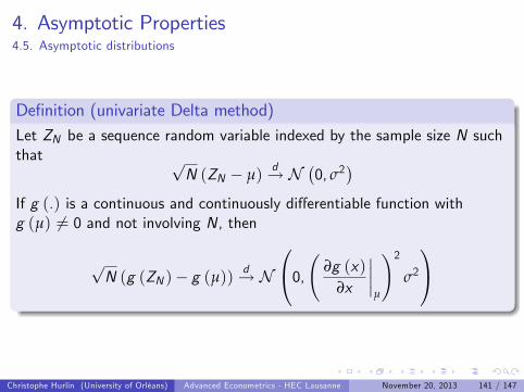
Denition (univariate Delta method)Let ZN be a sequence random variable indexed by the sample size N suchthat p

N (ZN µ)d! N

0, σ2

If g (.) is a continuous and continuously di¤erentiable function withg (µ) 6= 0 and not involving N, then

pN (g (ZN ) g (µ))

d! N

0@0, ∂g (x)∂x

µ

!2σ2

1A



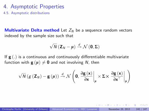
Multivariate Delta method Let ZN be a sequence random vectorsindexed by the sample size such that

pN (ZN µ)

d! N (0,Σ)

If g (.) is a continuous and continuously di¤erentiable multivariatefunction with g (µ) 6= 0 and not involving N, then

pN (g (ZN ) g (µ))

d! N 0,

∂g (x)∂x

µ

Σ ∂g (x)∂x>

µ

!



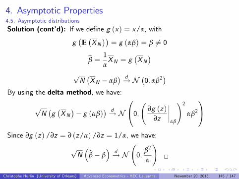
Example (Gamma distribution)Let X1, ..,XN denote a sequence of independent and identically distributedrandom variables. We assume that Xi Γ (α, β) (gamma distribution)with E (X ) = αβ and V (X ) = αβ2, α > 0, β > 0 and a pdf dened by:

fX (x ; α, β) =xα1 exp

x

β

Γ (α) βα , useless in this exercice, but for your culture

for 8x 2 [0,+∞[ , where Γ (α) =R ∞0 t

α1 exp (t) dt denotes theGamma function. We assume that α is known. Question: What is theasymptotic distribution of the estimator bβ dened by:

bβ = 1αN

N

∑i=1Xi



Solution: The estimator bβ is dened by:bβ = 1

αN

N

∑i=1Xi

Since X1, ..,XN are i .i .d . with E (X ) = αβ and V (X ) = αβ2, we canapply the LindebergLevy CLT, and we get immediately:

pNXN αβ

d! N0, αβ2



Solution (contd): If we dene g (x) = x/α, with

gEXN= g (αβ) = β 6= 0

bβ = 1αXN = g

XN

pNXN αβ

d! N0, αβ2

By using the delta method, we have:

pNgXN g (αβ)

d! N

0@0, ∂g (z)∂z

αβ

!2αβ2

1ASince ∂g (z) /∂z = ∂ (z/α) /∂z = 1/α, we have:

pNbβ β

d! N

0,

β2

α

!




1 Almost sure convergence2 Convergence in probability3 Law of large numbers: Khinchines and Kolmogorovs theorems4 Weakly and strongly consistent estimator5 Slutskys theorem6 Convergence in mean square7 Convergence in distribution8 Asymptotic distribution and asymptotic variance9 Lindeberg-Levy Central Limite Theorem (univariate and multivariate)10 Continuous mapping theorem11 Delta method


End of Chapter 1

Christophe Hurlin (University of Orléans)


Documents

Advanced Econometrics - HEC Lausanne Christophe Hurlin€¦ · 2. What is an Estimator? Question: What constitues a good estimator? 1 The search for good estimators constitutes much