©2018 Shelby Systems, Inc. Other brand and product names are trademarks or registered trademarks of the respective holders.

Advanced Excel Solutions

(Course #E215)

Presented by: Mark Crain Shelby Staff Trainer

2

Objective

The objective is to provide skills and tools that allow you to acquire new and different insights

into your data using Excel.

This session presents the following topics: Setting up Excel to obtain live information from ShelbyNext | Membership.

Use tables to create totals, averages, and visual sorting of large amounts of data.

Create maps based on membership or giving data.

3

Pulling Clean Data from ShelbyNext | Membership

Pulling data from ShelbyNext | Membership can be a hit and miss prospect. Some places allow

for exporting data into a convenient CSV file format. Others do not let you grab anything. This is

only partially true, if you know a specific feature of Excel called “Data From Web”.

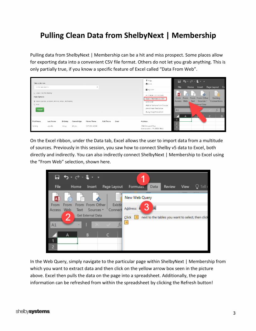
On the Excel ribbon, under the Data tab, Excel allows the user to import data from a multitude

of sources. Previously in this session, you saw how to connect Shelby v5 data to Excel, both

directly and indirectly. You can also indirectly connect ShelbyNext | Membership to Excel using

the “From Web” selection, shown here.

In the Web Query, simply navigate to the particular page within ShelbyNext | Membership from

which you want to extract data and then click on the yellow arrow box seen in the picture

above. Excel then pulls the data on the page into a spreadsheet. Additionally, the page

information can be refreshed from within the spreadsheet by clicking the Refresh button!

4

Getting a Clean Report The major side effect of this method of data extraction is that you get seemingly useless

information, such as what is shown below.

The file is available by emailing me, following the conference.

5

Excel Tables

An Excel Table is a special structure for managing information in lists or tables. To create quickly

an Excel Table, select any cell in the data, and use the keyboard shortcut CTRL + T

NOTE: For more information on Excel PivotTable functions, attend Excel Pivot Tables: Shelby v5,

Arena, & ShelbyNext Data (Course #E930) on Friday at 8:30am.

6

Key Advantages to Tables Dynamic ranges - Tables automatically expand to include new rows, behaving like dynamic

ranges. Perfect for charts and PivotTables.

Structure - Data appears in rows and columns without spaces, like a database.

Automatic update to formulas - New rows get existing formulas, with changes to existing

formulas occurring automatically.

Filters - Automatically available in a table.

Structured references - Easy to refer to table rows and columns without specific cell references.

The Total Row of a defined table can be plugged in with custom formulas as well

as selectable formulas that create sums, averages, counts and others.

7

In the table here, there have been some custom created formulas that look for the most

common values in 4 of the fields: Address, City, State, and Zip Code.

Address: =INDEX([Address],MODE(IF([Address]<>"",MATCH([Address],[Address],0))))

City: =INDEX([City],MODE(IF([City]<>"",MATCH([City],[City],0))))

State: =INDEX([State],MODE(IF([State]<>"",MATCH([State],[State],0))))

NOTE: Because the formulas above are array formulas, you must use the key

combination CTRL+Shift+Enter to get them to work.

For Zip Code, since the values could only be numerical, an additional formula could be used:

Zip Code: =MODE([Zip])

8

Creating Maps from Excel Data

Many long time Shelby v.5 customers may be familiar with a program from Microsoft called

MapPoint. This program had a great integration with v.5 that allowed you to view your

membership data in a visual format.

Unfortunately, this program was discontinued following the 2013 release edition. However,

built into Excel 2016 (and downloadable free as an add-on for earlier Excel versions) is a

function called 3D Maps (2016) / PowerMap (2013 and earlier).

Using a basic Excel export from any Shelby program, you can quickly and easily create an

interactive map, like the one shown below:

9

Tables and Maps Scenario

There is a request from our leadership to analyze the locations in the city from where our

members come to church.

To start, download your membership data from v.5/Arena/ShelbyNext | Membership.

Knowing your data is key in this process. If your normal data entry procedures involve using Zip

+ 4, you may want to consider adding an additional column for Zip and use the formula below

to strip out the base zip code:

=LEFT([@[Zip Code]],5)

Select any cell in the data and press CTRL + T to turn the data into a table.

10

Excel should automatically identify the

bounds of your data, but always

double check! If your data has a

header row, make sure the My table

has headers check box is selected.

The Total Row is a great addition to most

any Excel table. It allows you to create

custom formulas and use stock formulas

for the full column above that adjust

automatically on the inclusion of new

rows in the table. Ensure that Header

Row, Banded Rows, and Filter Button are

also selected.

If the goal is to simply filter the data to find specifics, such as missing email addresses, all the

male members, or the records listed as sons or daughters, you could use the filters found in the

header row to see exactly those things or some combination of your choosing.

However, our leadership would like to see the information on a map.

If you have not yet saved this file in .xlsx format, do so now. The Maps utility can only be used

in a full Excel workbook.

In Excel 2016, under the Insert tab, click on

the 3D Map button, located in the Insert tab

of Microsoft Excel.

11

The changes you will be making are using the

Layer Pane.

Location controls the level of detail used for

the data. In most cases, a standard Zip Code

is the best choice here.

Height/Size/Value is the next variable and

controls the height of the column, size of the

bubble, etc.

Category allows for further division of the

data, into a stacked column or pie chart.

Additional layers can be added for further information display. Simplicity is key to proper

understanding of these types of data displays. Too many different columns, areas, circles, etc.

only create confusion and makes the display lose significant value.

For our purposes, you are setting the layer as a Stacked Column layer, using Zip as the Location,

Zip (Count – Not Blank) as the Height, and Last Name as the Category.

12

A nice chart, but if you add a second layer with the same Location and Value settings as before,

but change the chart visualization to Region, you get the following:

The difference is staggering and highly informative.

13

Stacked Formulas

=IF(‘Worked With Code’A1=”yes”,”Awesome!”,”This will make sense soon.”)

In many Excel classes, you start to learn basic formulas, like SUM, AVERAGE, etc. In an advanced

class, you find out that formulas are like the movie Inception. One can be inside another inside

another inside another…….

=IF($C2="","",(VLOOKUP($C2,'Full Export Members Mail Grp'!$B$2:$ZX$99999,16,FALSE)))

=IFNA(IF('Processing (Do Not Change)'!K2<0,"Pledge Paid",'Processing (Do Not

Change)'!K2),0)

=IFNA(VLOOKUP(B7,YEARAWORK!$C$1:$D$999,2,FALSE),0)

You can reference the results of other formulas, on different sheets, in different workbooks, to

create new solutions to new formulas in new sheets of new workbooks. Mind blown, I know!

Cell references, like A1 or !C!17, are pretty commonplace. Even referencing other sheets in the

same workbook is done with some regularity now, i.e. =IF(‘Worked With Code’A1….

There is a special formula, however, that you need to use in order to create a reference to

another workbook. And it is the INDIRECT formula.

=INDIRECT("'["&workbook&"]"&sheet&"'!"&ref)

One caveat, the other workbook has to be OPEN in order for this to work, which is only mildly

inconvenient. So what about a file that isn’t open?

Well…….

=INDEX('E:\Excel file\[test.xlsx]Sheet2'!A:A,2,1)

In the formula, E:\Excel file\ is the full file path of the unopened workbook, test.xlsx is the name

of the workbook, Sheet2 is the sheet name which contains the cell value you need to reference

from, and A:A,2,1 means the cell A2 is referenced in the closed workbook. You can change them

based on your needs.

14

Q&A

Class Discussion

Mark Crain Shelby Staff Trainer

Mark.Crain@shelbyinc.com

photo

Presenter bio inserted here during Production Review