ADVANCED GCE UNIT 4769/01MATHEMATICS (MEI)

Statistics 4

TUESDAY 5 JUNE 2007 Afternoon

Time: 1 hour 30 minutesAdditional Materials:

Answer booklet (8 pages)Graph paperMEI Examination Formulae and Tables (MF2)

INSTRUCTIONS TO CANDIDATES

• Write your name, centre number and candidate number in the spaces provided on the answer booklet.

• Answer any three questions.

• You are permitted to use a graphical calculator in this paper.

• Final answers should be given to a degree of accuracy appropriate to the context.

INFORMATION FOR CANDIDATES

• The number of marks is given in brackets [ ] at the end of each question or part question.

• The total number of marks for this paper is 72.

ADVICE TO CANDIDATES

• Read each question carefully and make sure you know what you have to do before starting your answer.

• You are advised that an answer may receive no marks unless you show sufficient detail of the working toindicate that a correct method is being used.

This document consists of 4 printed pages.

© OCR 2007 [Y/102/2659] OCR is an exempt Charity [Turn over

2

Option 1: Estimation

1 The random variable X has the continuous uniform distribution with probability density function

f(x) = 1θ

, 0 ≤ x ≤ θ,

where θ (θ > 0) is an unknown parameter.

A random sample of n observations from X is denoted by X1, X2, . . . , Xn, with sample mean

X = 1n

n

∑i=1

Xi.

(i) Show that 2X is an unbiased estimator of θ . [4]

(ii) Evaluate 2X for a case where, with n = 5, the observed values of the random sample are 0.4, 0.2,1.0, 0.1, 0.6. Hence comment on a disadvantage of 2X as an estimator of θ. [4]

For a general random sample of size n, let Y represent the sample maximum, Y =max(X1, X2, . . . , Xn).You are given that the probability density function of Y is

g(y) = nyn−1

θn , 0 ≤ y ≤ θ.

(iii) An estimator kY is to be used to estimate θ, where k is a constant to be chosen. Show that themean square error of kY is

k2E(Y2) − 2kθE(Y) + θ2

and hence find the value of k for which the mean square error is minimised. [12]

(iv) Comment on whether kY with the value of k found in part (iii) suffers from the disadvantageidentified in part (ii). [4]

© OCR 2007 4769/01 Jun07

3

Option 2: Generating Functions

2 The random variable X has the binomial distribution with parameters n and p, i.e. X ∼ B(n, p).(i) Show that the probability generating function of X is G(t) = (q + pt)n, where q = 1 − p. [4]

(ii) Hence obtain the mean µ and variance σ2 of X. [6]

(iii) Write down the mean and variance of the random variable Z = X − µσ

. [1]

(iv) Write down the moment generating function of X and use the linear transformation result to showthat the moment generating function of Z is

MZ(θ) = (qe− pθ√

npq + peqθ√npq )

n

. [5]

(v) By expanding the exponential terms in MZ(θ), show that the limit of MZ(θ) as n → ∞ is eθ2/2.

You may use the result limn→∞(1 + y + f(n)

n)

n= ey provided f(n) → 0 as n → ∞. [4]

(vi) What does the result in part (v) imply about the distribution of Z as n → ∞? Explain yourreasoning briefly. [3]

(vii) What does the result in part (vi) imply about the distribution of X as n → ∞? [1]

Option 3: Inference

3 An engineering company buys a certain type of component from two suppliers, A and B. It is importantthat, on the whole, the strengths of these components are the same from both suppliers. The companycan measure the strengths in its laboratory. Random samples of seven components from supplier Aand five from supplier B give the following strengths, in a convenient unit.

Supplier A 25.8 27.4 26.2 23.5 28.3 26.4 27.2

Supplier B 25.6 24.9 23.7 25.8 26.9

The underlying distributions of strengths are assumed to be Normal for both suppliers, with variances2.45 for supplier A and 1.40 for supplier B.

(i) Test at the 5% level of significance whether it is reasonable to assume that the mean strengthsfrom the two suppliers are equal. [10]

(ii) Provide a two-sided 90% confidence interval for the true mean difference. [4]

(iii) Show that the test procedure used in part (i), with samples of sizes 7 and 5 and a 5% significancelevel, leads to acceptance of the null hypothesis of equal means if −1.556 < x − y < 1.556, wherex and y are the observed sample means from suppliers A and B. Hence find the probability of aType II error for this test procedure if in fact the true mean strength from supplier A is 2.0 unitsmore than that from supplier B. [7]

(iv) A manager suggests that the Wilcoxon rank sum test should be used instead, comparing themedian strengths for the samples of sizes 7 and 5. Give one reason why this suggestion might besensible and two why it might not. [3]

© OCR 2007 4769/01 Jun07 [Turn over

4

Option 4: Design and Analysis of Experiments

4 An agricultural company conducts a trial of five fertilisers (A, B, C, D, E) in an experimental field at itsresearch station. The fertilisers are applied to plots of the field according to a completely randomiseddesign. The yields of the crop from the plots, measured in a standard unit, are analysed by the one-wayanalysis of variance, from which it appears that there are no real differences among the effects of thefertilisers.

A statistician notes that the residual mean square in the analysis of variance is considerably larger thanhad been anticipated from knowledge of the general behaviour of the crop, and therefore suspects thatthere is some inadequacy in the design of the trial.

(i) Explain briefly why the statistician should be suspicious of the design. [2]

(ii) Explain briefly why an inflated residual leads to difficulty in interpreting the results of the analysisof variance, in particular that the null hypothesis is more likely to be accepted erroneously. [3]

Further investigation indicates that the soil at the west side of the experimental field is naturally morefertile than that at the east side, with a consistent ‘fertility gradient’ from west to east.

(iii) What experimental design can accommodate this feature? Provide a simple diagram of theexperimental field indicating a suitable layout. [4]

The company decides to conduct a new trial in its glasshouse, where experimental conditions can becontrolled so that a completely randomised design is appropriate. The yields are as follows.

Fertiliser A Fertiliser B Fertiliser C Fertiliser D Fertiliser E

23.6 26.0 18.8 29.0 17.718.2 35.3 16.7 37.2 16.532.4 30.5 23.0 32.6 12.820.8 31.4 28.3 31.4 20.4

[The sum of these data items is 502.6 and the sum of their squares is 13 610.22.]

(iv) Construct the usual one-way analysis of variance table. Carry out the appropriate test, using a5% significance level. Report briefly on your conclusions. [12]

(v) State the assumptions about the distribution of the experimental error that underlie your analysisin part (iv). [3]

Permission to reproduce items where third-party owned material protected by copyright is included has been sought and cleared where possible. Every reasonableeffort has been made by the publisher (OCR) to trace copyright holders, but if any items requiring clearance have unwittingly been included, the publisher will bepleased to make amends at the earliest possible opportunity.

OCR is part of the Cambridge Assessment Group. Cambridge Assessment is the brand name of University of Cambridge Local Examinations Syndicate (UCLES),which is itself a department of the University of Cambridge.

© OCR 2007 4769/01 Jun07

Mark Scheme 4769June 2007

88

4769 Mark Scheme June 2007

1)

f (x) = θ1

0 x ≤ ≤ θ

2][E θ

=X B1 Write-down, or by symmetry, or by

integration. (i)

][E2][E2]2[E XXX == = θ ∴ unbiased

M1 A1

4 E1

∑ x = 2.3 ∴ x = 53.2

= 0.46 ∴2 x = 0.92 B1 (ii)

But we know θ ≥ 1 E1 ∴ estimator can give nonsense answers, E2 (E1, E1)

i.e. essentially useless 4 (iii)

Y = max{Xi}, g(y) = n

nnyθ

1−

0 ≤ y ≤ θ

MSE (kY) = = ])[(E 2θ−kY M1

= ] 2[E 222 θθ +− YkYk 222 ][E 2][E θθ +− YkYk 1 BEWARE PRINTED ANSWER

dkdMSE

= M1

0][E 2][E2 2 =− YYk θ M1

for ][E][E

2YYk θ

= A1

2

2MSEdk

d= 0][E2 2 >Y ∴ this is a minimum

M1

][E Y = n

nnyθ

θ

∫0

dy = 1

1

+

+

nn n

n

θθ

= 1+n

nθ

M1 A1

][E 2Y = ∫

θ

0n

nnyθ

1+

dy = 2

2

+

+

nn n

n

θθ

= 2

2

+nnθ

M1 A1

M1 A1

∴minimising k = θ

1+nnθ

2

2θn

n +12

++

nn

= 12

(iv) With this k, kY is always greater than the sample maximum So it does not suffer from the disadvantage in part (ii)

E2 E2

(E1 E1) (E1 E1)

4

89

4769 Mark Scheme June 2007 2(i)

M1

xnxn

x

X pptxn

tt −

=

−⎟⎟⎠

⎞⎜⎜⎝

⎛== ∑ )1()(][E)(G

0

= nptp ])1[( +− 2 Available as B2 for write-down or as 1+1 for algebra

nptq )( += 1 4

)1(G′=μ 1)()(G −+=′ nptqnpt 1 (ii)

npnp =×=′ 1)1(G 1 22 )1(G μμσ −+′′=

22 )()1()(G −+−=′′ nptqpnnt1

2)1()1('G' pnn −= 1 222222 pnnpnppn −+−=∴σ M1 npqnpnp =+−= 2 1 6

(iii) σ

μ−=

XZ Mean 0, Variance 1 B1

For BOTH

1

(iv) npeqe )()(G)(M θθθ +== 1

baXZ += with:

npqa 11

==σ

and qnpb −=−=

σμ

)(M)(M θθ θ ae Xb

Z =

M1

=

⎟⎟

⎠

⎞

⎜⎜

⎝

⎛+=∴

−n

npqqnp

Z peqeθθ

θ1

)(M

n

npqp

npqp

peqe⎟⎟

⎠

⎞

⎜⎜

⎝

⎛+

−− θθ 1

1 1 1

BEWARE PRINTED ANSWER

5

(v) ++−=

npqqp

npqqpqZ 2

()(M22θθθ

terms in 23−n , , ………….. + 2−n

n

npqpq

npqpqp )

2

22

+++θθ

=

→++ n

n)

21(

2θ

22θ

e

M1 M1 1 1

For expansion of exponential terms For indication that these can be neglected as . Use of result given in question

∞→n

4

90

4769 Mark Scheme June 2007 (vi) N(0,1)

Because 22θe is the mgf of N(0,1)

and the relationship between distributions and

their mgfs is unique

1

E1 E1

3

(vii) “Unstandardising”, ie ),(N 2σμ ),(N npqnp 1 Parameters need to be given. 1

91

4769 Mark Scheme June 2007 3(i)

BAH μμ =:0

BAH μμ ≠:1 Where Aμ , Bμ are the population means

1 1

Do NOT allow YX = or similar Accept absence of “population” if correct notation μ is used. Hypotheses stated verbally must include the word “population”.

Test statistic

=+

−

540.1

745.2

38.254.26

285.17937.063.0

02.1=

=

M1 M1 M1 A1

Numerator Denominator two separate terms correct

Refer to N(0,1) Double-tailed 5% point is 1.96 Not significant No evidence that the population means differ

1 1 1 1

No FT if wrong No FT if wrong

10

(ii) CI ( for Aμ – Bμ ) is ±02.1

×645.1 =7937.0

=± 3056.102.1 (– 0.2856, 2.3256)

M1 B1 M1 A1 cao

Zero out of 4 if not N(0,1)

4

(iii) 0H is accepted if –1.96< test statistic < 1.96

i.e. if 96.17937.0

96.1 <−

<−yx

i.e. if 556.1556.1 <−<− yx

M1 M1 A1

SC1 Same wrong test can get M1,M1,A0. SC2 Use of 1.645 gets 2 out of 3. BEWARE PRINTED ANSWER

In fact, )7937.0,2(N~ 2YX − So we want

)556.1)7937.0,2(N556.1(P 2 <<− =

⎟⎠⎞

⎜⎝⎛ −

<<−−

7937.02556.1)1,0(N

7937.02556.1P =

2879.0)5594.0)1,0(N48.4(P =−<<−

M1

M1 M1 A1 cao

7

Standardising

(iv) Wilcoxon would give protection if assumption of Normality is wrong.

E1

Wilcoxon could not really be applied if underlying variances are indeed different.

E1

Wilcoxon would be less powerful (worse Type II error behaviour) with such small samples if Normality is correct.

E1

3

92

4769 Mark Scheme June 2007 4 (i) There might be some consistent source of plot-

to-plot variation that has inflated the residual and which the design has failed to cater for.

E2 E1 – Some reference to extra variation. E1 – Some indication of a reason.

2

(ii) Variation between the fertilisers should be compared with experimental error.

If the residual is inflated so that it measures

more than experimental error, the comparison of between - fertilisers variation with it is less likely to reach significance.

E1 E2

(E1, E1)

3

(iii) Randomised blocks

SPECIAL CASE: Latin Square 42

(1, E1)

C B A D E

. . .

. . .

1 E1 E1 E1

Blocks (strips) clearly correctly oriented w.r.t. fertiliser gradient. All fertilisers appear in a block. Different (random) arrangements in the blocks.

4

(iv) Totals are: 95.0 123.2 86.8 130.2 67.4 (each from sample of size 4) Grand total 502.6

“Correction factor” CF = =20

6.502 212630.338

Total SS = 13610.22 – CF = 979.882 Between fertilisers SS =

44.67...

40.95 22

++ – CF =

13308.07 – CF = 677.732 Residual SS (by subtraction) = 979.882 – 677.732=302.15

M1 M1 A1

For correct method for any two If each calculated SS is correct

Source of variation SS df MS MS Ratio Between fertiliser 677.732 4 169.433 8.41 Residual 302.15 15 20.143 Total 979.882 19

M1 M1 1,A1 1

Refer to F4, 15 1 No FT if wrong -upper 5% point is 3.06 1 No FT if wrong Significant

- seems effects of fertilisers are not all the same 1 1

12

(vii) Independent N (0, σ2 [constant])

1 1 1

3

93

Report on the Units taken in June 2007 4769: Statistics 4 General Comments This is the second time that the new-specification Statistics 4 module has been sat. Although the entry is small, it is pleasing that the opportunity to proceed to high levels in the applied mathematics strands is still available. There was some extremely good work, and only a little very poor work. The paper consists of four questions, each within a defined "option" area of the specification. The rubric requires that three be attempted. All four questions received many attempts – another encouraging feature, as it indicates that centres and candidates are spreading their work over all the options. Sadly there were again cases of "faking" of answers that were given within the questions. This was discussed at some length in last year's report. This year, I will merely reiterate that it is entirely unacceptable. Comments on Individual Questions 1 This was on the "estimation" option. It consisted of comparison of two estimators of θ

for the uniform distribution on (0, θ). The first of those estimators was X2 . Most candidates showed quickly enough that it was unbiased, but surprisingly many did not spot that, with the sample data given, its value was 0.92 even though we knew that θ must be at least 1, thus making it a fairly useless estimator! Candidates tended instead to struggle in making unconvincing comments about its variance. The question then moved on to a new estimator whose mean square error was to be found; this was usually done fairly successfully, some candidates being much more efficient in their work than others, and some not really being able to cope at all. Candidates who had spotted the key disadvantage of the first estimator were usually able to see that the new estimator could not possibly suffer from it, but others struggled to find anything sensible to say.

2 This was on the "generating functions" option. It led candidates through the steps of

proving that the limiting distribution of the B(n, p) random variable as n → ∞ is N(np, npq). Most candidates proceeded thoroughly and carefully through the technical mathematical work, much of which should have been standard bookwork. However, surprisingly many could not simply write down 0 and 1 for the mean and variance in part (iii). In part (iv), several candidates were rescued, with greater or less legitimacy, by the provision in the question of the answer. In part (v), some candidates did not realise that the first step towards the limiting result was to expand the exponential terms from part (iv). Most, however, did this quite well, sometimes not being entirely convincing in their use of the result given in the question (simply averring that their version of the f(n) in that result was actually equal to zero rather missed the point).

53

Report on the Units taken in June 2007

3 This question was on the "inference" option. It was based on an unpaired Normal test, proceeding to consideration of Type II error. Mostly the test and confidence interval (parts (i) and (ii)) were well done, though some of the usual errors did appear from time to time. Part (iii) met with mixed success; it was done very well by some candidates, whereas others fell by the wayside en route. Surprisingly many failed to consider both "tails" in finding the last probability; though one of them turns out to be negligible in the extreme, this cannot be known until there has been some investigation of it! A variety of suggestions in favour of and against the Wilcoxon alternative came forward in part (iv).

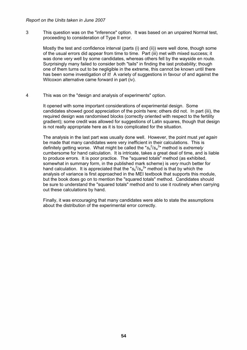
4 This was on the "design and analysis of experiments" option.

It opened with some important considerations of experimental design. Some candidates showed good appreciation of the points here; others did not. In part (iii), the required design was randomised blocks (correctly oriented with respect to the fertility gradient); some credit was allowed for suggestions of Latin squares, though that design is not really appropriate here as it is too complicated for the situation. The analysis in the last part was usually done well. However, the point must yet again be made that many candidates were very inefficient in their calculations. This is definitely getting worse. What might be called the "sb

2/sw2" method is extremely

cumbersome for hand calculation. It is intricate, takes a great deal of time, and is liable to produce errors. It is poor practice. The "squared totals" method (as exhibited, somewhat in summary form, in the published mark scheme) is very much better for hand calculation. It is appreciated that the "sb

2/sw2" method is that by which the

analysis of variance is first approached in the MEI textbook that supports this module, but the book does go on to mention the "squared totals" method. Candidates should be sure to understand the "squared totals" method and to use it routinely when carrying out these calculations by hand. Finally, it was encouraging that many candidates were able to state the assumptions about the distribution of the experimental error correctly.

54