Embed Size (px)
Citation preview
Advanced International Trade:Theory and Evidence
(c) Robert C. FeenstraUniversity of California, Davis, and
National Bureau of Economic ResearchAugust 2002
Contents:
Forward
1. Preliminaries: Two-Sector Models
2. The Heckscher-Ohlin Model
3. Many Goods and Factors
4. Trade in Intermediate Inputs and Wages
5. Increasing Returns and the Gravity Equation
6. Gains from Trade and Regional Agreements
7. Import Tariffs and Dumping
8. Import Quotas and Export Subsidies
9. Political Economy of Trade Policy
10. Trade and Endogenous Growth
11. Multinationals and Organization of the Firm
Appendix A. Price, Productivity and Terms of Trade Indexes
Appendix B. Discrete Choice Models
References

2
Foreword
This book is intended for a graduate course in international trade. I assume that
all readers have completed graduate courses in microeconomics and econometrics. My
goal is to bring the reader from that common point up to the most recent research in
international trade: in both theory and empirical work. This is not intended to be a
difficult book, and the mathematics used should be accessible to any graduate student.
The material covered will give the reader the skills needed to understand the latest
articles and working papers in the field.
At the same time, I am aware that many readers will become teachers in the field,
especially at the undergraduate level. I feel that it is suitable, then, to start each chapter
by introducing simple graphical techniques that can be used in teaching. Following this, I
move towards the equations for each model. A set of problems at the end of each chapter
give the reader some experience in manipulating these equations. An instructors manual
that accompanies this book provides solutions to the problems.1 In addition, I have
included empirical exercises that replicate the results in some chapters. Completing all of
these could be the topic for a second course, but even in a first course there will be a
payoff to trying some exercises. The data and programs for these can be found on my
home page and also at the website www.internationaldata.org.2
A word on notation. I consistently use subscripts to refer to goods or factors,
whereas superscripts refer to consumers or countries. In general, then, subscripts refer to
commodities and superscripts refer to agents. The index used (h, i, j, k, l , m, or n) will
1 Faculty wishing to obtain the instructors manual should contact Princeton University Press.2 The programs for the empirical exercises are provided in STATA. Readers not familiar with STATA areencouraged to complete the web course developed by James Levinsohn and available at:www.psc.isr.umich.edu/saproject .
3
depend on the context. The symbol “c” is used for both costs and consumption, though in
some chapters I instead use “d(p)” for consumption to avoid confusion. The output of
firms is consistently denoted by “y” and exports are denoted by “x”. Upper-case letters
are used in some cases to denote vectors or matrixes, and in other cases to denote the
number of goods (N), factors (M), households (H) or countries (C), and sporadically
elsewhere. The symbols α and β are used generically for intercept and slope coefficients,
including fixed and marginal labor costs.
The contents of several chapters included here have been previously published.
Chapters 4 and 5 are revisions from articles appearing in Kwan Choi and James Harrigan,
eds., Handbook of International Trade (Basil Blackwell, 2003) and the Scottish Journal
of Economics, respectively. Some material from chapters 7 – 9 has appeared in articles
published in the Journal of International Economics and the Quarterly Journal of
Economics, and material from chapter 10 has appeared in the Journal of Development
Economics and the American Economic Review.

Feenstra, Advanced International Trade
Chapter 1: Preliminaries: Two-Sector Models
We begin our study of international trade with the classic Ricardian model, which has
two goods and one factor (labor). The Ricardian model introduces us to the idea that
technological differences across countries matter. In comparison, the Heckscher-Ohlin model
dispenses with the notion of technological differences and instead show how factor endowments
form the basis for trade. While this may be fine in theory, it performs very poorly in practice: as
we show in the next chapter, the Heckscher-Ohlin model is hopelessly inadequate as an
explanation for historical or modern trade patterns unless we allow for technological differences
across countries. For this reason, the Ricardian model is as relevant today as it has always been.
Our treatment of it in this chapter is a simple review of undergraduate material, but we will have
the opportunity to refer to this model again at various places throughout the book.
After reviewing the Ricardian model, we turn to the two-good, two-factor model which
occupies most of this chapter and forms the basis of the Heckscher-Ohlin model. We shall
suppose that the two goods are traded on international markets, but do not allow for any
movements of factors across borders. This reflects the fact that the movement of labor and
capital across countries is often subject to controls at the border and generally much less free
than the movement of goods. Our goal in the next chapter will be to determine the pattern of
international trade between countries. In this chapter, we simplify things by focusing primarily
on one country, treating world prices as given, and examine the properties of this two-by-two
model. The student who understands all the properties of this model has already come a long
way in his or her study of international trade.
Feenstra, Advanced International Trade1-2
Ricardian Model
Indexing goods by the subscript i, let ai denote the labor needed per unit of production of
each good at home, while *ia is the labor need per unit of production in the foreign country,
i=1,2. The total labor force at home is L and abroad is L*. Labor is perfectly mobile between
the industries in each country, but immobile across countries. This means that both goods are
produced in the home country only if the wages earned in the two industries are the same. Since
the marginal product of labor in each industry is 1/ai , wages are equalized across industries if
and only if p1/a1 = p2/a2 , where pi is the price in each industry. Letting p = p1/p2 denote the
relative price of good 1 (using good 2 as the numeraire), this condition is p = a1/a2.
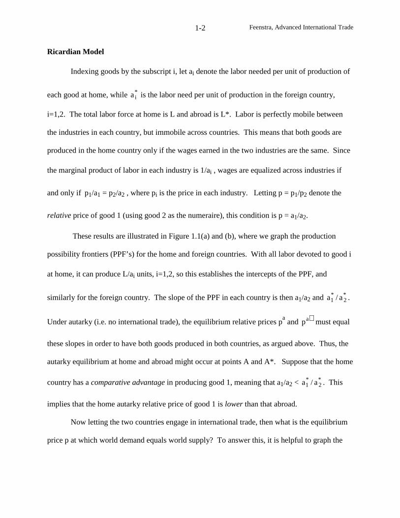
These results are illustrated in Figure 1.1(a) and (b), where we graph the production
possibility frontiers (PPF’s) for the home and foreign countries. With all labor devoted to good i
at home, it can produce L/ai units, i=1,2, so this establishes the intercepts of the PPF, and
similarly for the foreign country. The slope of the PPF in each country is then a1/a2 and *2
*1 a/a .
Under autarky (i.e. no international trade), the equilibrium relative prices pa
and ∗ap must equal
these slopes in order to have both goods produced in both countries, as argued above. Thus, the
autarky equilibrium at home and abroad might occur at points A and A*. Suppose that the home
country has a comparative advantage in producing good 1, meaning that a1/a2 < *2
*1 a/a . This
implies that the home autarky relative price of good 1 is lower than that abroad.
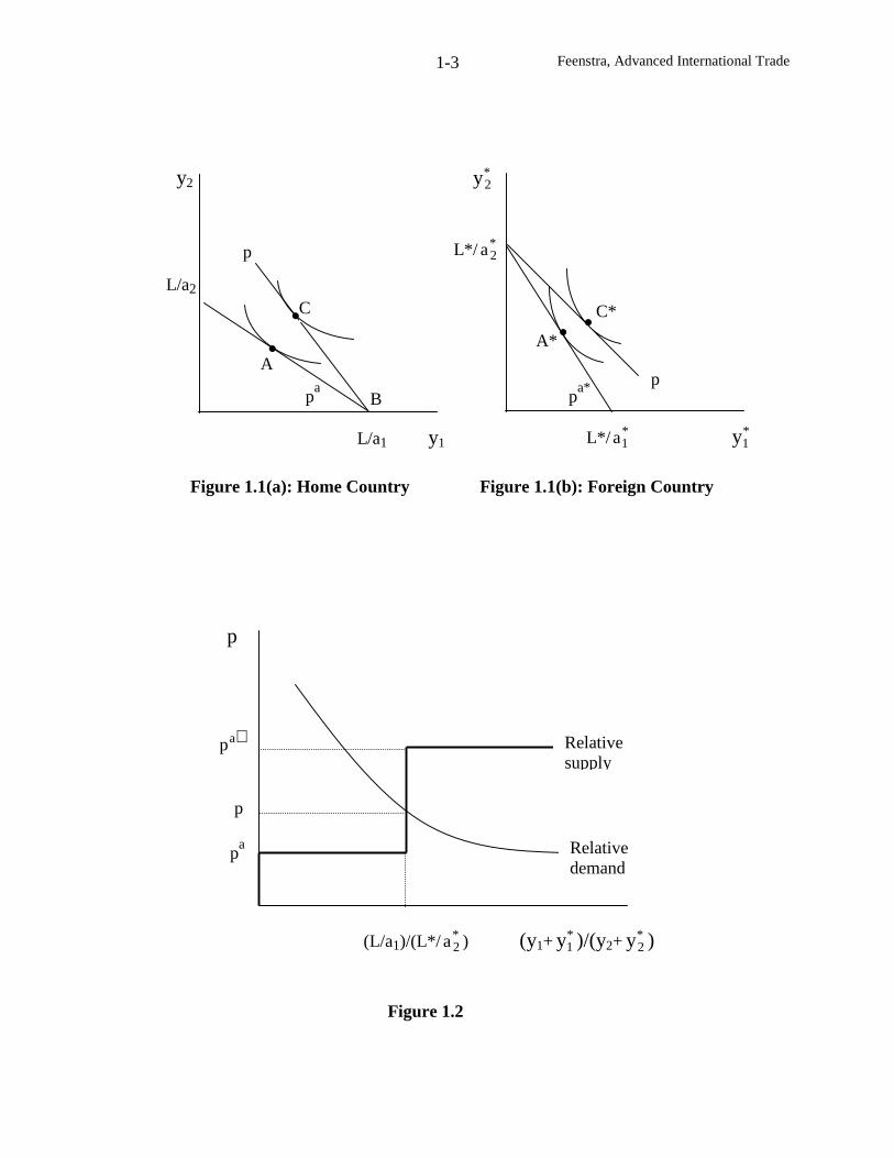
Now letting the two countries engage in international trade, then what is the equilibrium
price p at which world demand equals world supply? To answer this, it is helpful to graph the
Feenstra, Advanced International Trade1-3
B
B*
Figure 1.1(a): Home Country Figure 1.1(b): Foreign Country
A
L/a1 y1
y2
L/a2
C
Relativesupply
(L/a1)/(L*/ *2a ) (y1+ *
1y )/(y2+ *2y )
p
∗ap
p
pa Relative
demand
Figure 1.2
A*
L*/ *1a *
1y
C*
*2y
L*/ *2a
pa*
pa p
p
Feenstra, Advanced International Trade1-4
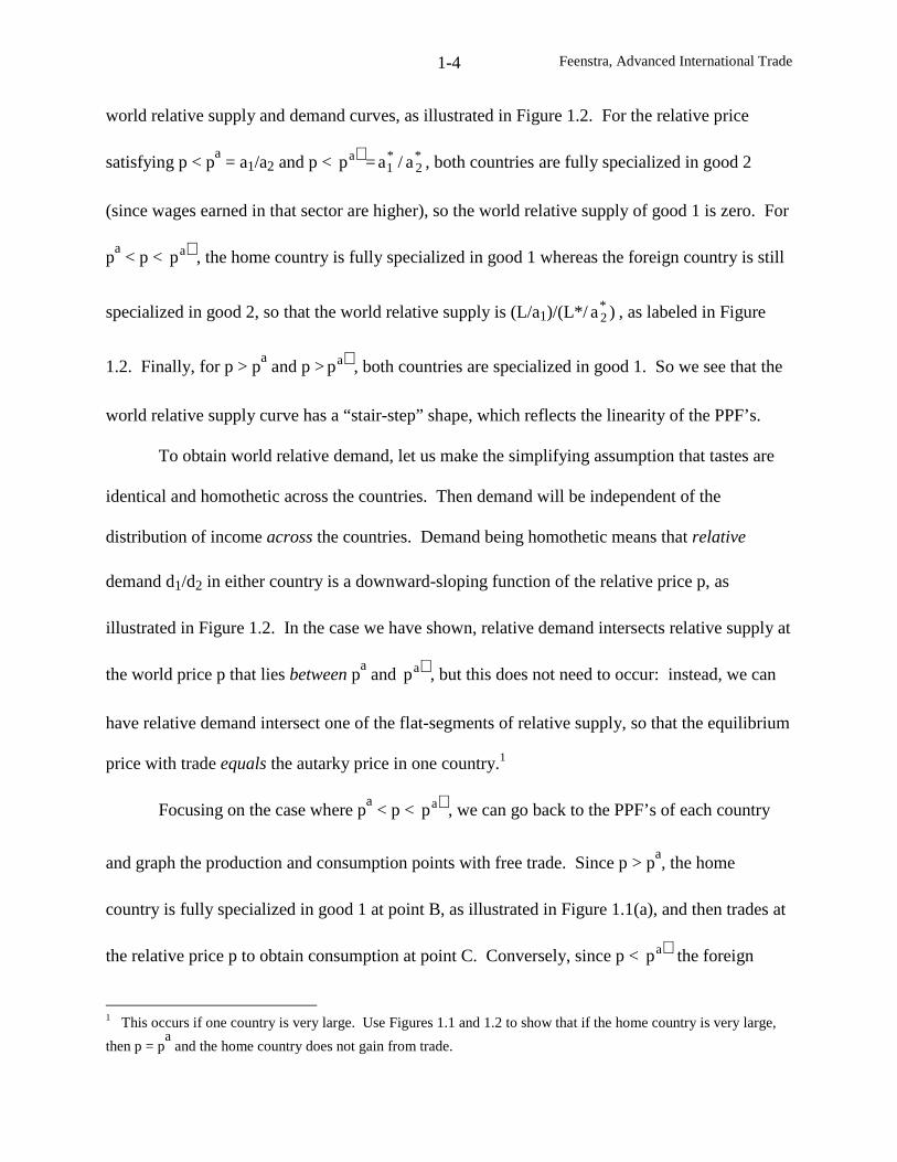
world relative supply and demand curves, as illustrated in Figure 1.2. For the relative price
satisfying p < pa
= a1/a2 and p < ∗ap = *2
*1 a/a , both countries are fully specialized in good 2
(since wages earned in that sector are higher), so the world relative supply of good 1 is zero. For
pa
< p < ∗ap , the home country is fully specialized in good 1 whereas the foreign country is still
specialized in good 2, so that the world relative supply is (L/a1)/(L*/ )a*2 , as labeled in Figure
1.2. Finally, for p > pa
and p > ∗ap , both countries are specialized in good 1. So we see that the
world relative supply curve has a “stair-step” shape, which reflects the linearity of the PPF’s.
To obtain world relative demand, let us make the simplifying assumption that tastes are
identical and homothetic across the countries. Then demand will be independent of the
distribution of income across the countries. Demand being homothetic means that relative
demand d1/d2 in either country is a downward-sloping function of the relative price p, as
illustrated in Figure 1.2. In the case we have shown, relative demand intersects relative supply at
the world price p that lies between pa
and ∗ap , but this does not need to occur: instead, we can
have relative demand intersect one of the flat-segments of relative supply, so that the equilibrium
price with trade equals the autarky price in one country.1
Focusing on the case where pa
< p < ∗ap , we can go back to the PPF’s of each country
and graph the production and consumption points with free trade. Since p > pa, the home
country is fully specialized in good 1 at point B, as illustrated in Figure 1.1(a), and then trades at
the relative price p to obtain consumption at point C. Conversely, since p < ∗ap the foreign
1 This occurs if one country is very large. Use Figures 1.1 and 1.2 to show that if the home country is very large,
then p = pa
and the home country does not gain from trade.
Feenstra, Advanced International Trade1-5
country is fully specialized in the production of good 2 at point B*, in Figure 1.1(b), and then
trades at the relative price p to obtain consumption at point C*. Clearly, both countries are better
off under free trade than they were in autarky: trade has allowed them to obtain a consumption
point that is above the PPF.
Notice that the home country exports good 1, which is in keeping with its comparative
advantage in the production of that good, a1/a2 < *2
*1 a/a . Thus, trade patterns are determined by
comparative advantage, which is a deep insight from the Ricardian model. This occurs even if
one country has an absolute disadvantage in both goods, such as a1 > *1a and a2 > *
2a , so that
more labor is needed per unit of production of either good at home than abroad. The reason that
it is still possible for the home country to export is that its wages will adjust to reflect its
productivities: under free trade, its wages are lower than those abroad.2 Thus, while trade
patterns in the Ricardian model are determined by comparative advantage, the level of wages
across countries is determined by absolute advantage.
Two-Good, Two-Factor Model
Focusing now on a single country, we will suppose that it produces two goods with the
production functions )K,L(fy iiii = , i=1,2, where yi is the output produced using labor Li and
capital Ki. These production functions are assumed to be increasing, concave, and homogeneous
of degree one in the inputs (Li, Ki ).3 The last assumption means that there is constant returns to
2 The home country exports good 1, so wages earned with free trade are w = p/a1. Conversely, the foreign country
exports good 2 (the numeraire), so wages earned there are w* = *2a/1 > *
1a/p , where the inequality follow since p <
*2a/
*1a in the equilibrium being considered. Then using a1 > *
1a , we obtain w = p/a1 < *1a/p < w*.
3 Students not familiar with these terms are referred to problems 1.1 and 1.2.
Feenstra, Advanced International Trade1-6
scale in the production of each good. This will be a maintained assumption for the next several
chapters, but it should be pointed out that it is rather restrictive. It has long been thought that
increasing returns to scale might be an important reason to have trade between countries: if a
firm with increasing returns is able to sell in a foreign market, this expansion of output will bring
a reduction in its average costs of production, which is an indication of greater efficiency.
Indeed, this was a principal reason that Canada entered into a free trade agreement with the
United States in 1989: to give its firms free access to the large American market. We will return
to these interesting issues in chapter 5, but for now, ignore increasing returns to scale.
We will assume that labor and capital are assumed to be fully mobile between the two
industries, so we are taking a “long run” point of view. Of course, the amount of factors
employed in each industry is constrained by the endowments found in the economy. These
resource constraints are stated as:
,KKK
,LLL
21
21
≤+≤+
(1.1)
where the endowments L and K are fixed. Maximizing the amount of good 2, )K,L(fy 2222 = ,
subject to a given amount of good 1, )K,L(fy 1111 = , and the resource constraints in (1.1) gives
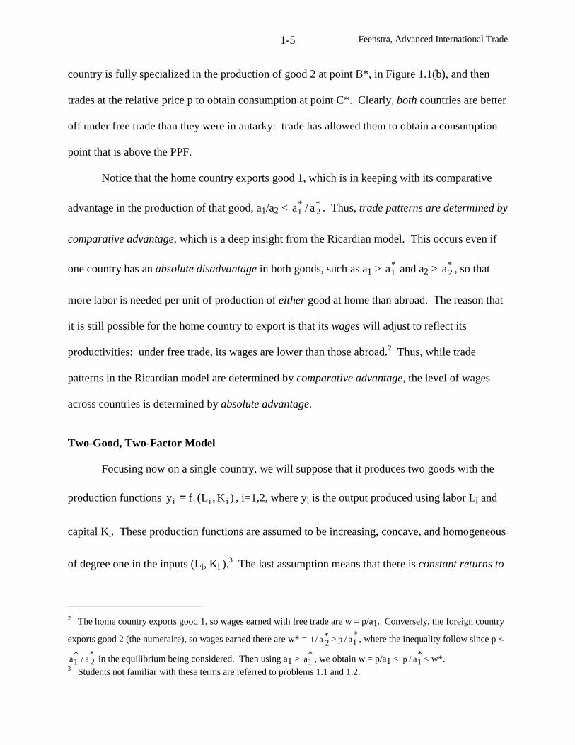
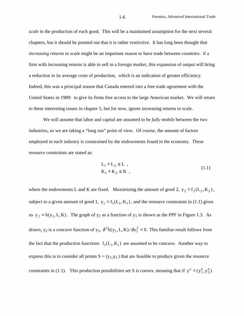
us )K,L,y(hy 12 = . The graph of y2 as a function of y1 is shown as the PPF in Figure 1.3. As
drawn, y2 is a concave function of y1, .0y/)K,L,y(h 211
2 <∂∂ This familiar result follows from
the fact that the production functions )K,L(f iii are assumed to be concave. Another way to
express this is to consider all points S = (y1,y2 ) that are feasible to produce given the resource
constraints in (1.1). This production possibilities set S is convex, meaning that if )y,y(y a2
a1
a =
Feenstra, Advanced International Trade1-7
λya +(1-λ)yb
ya=(y1a,y2
a)
yb=(y1b,y2
b)
PP Frontier
y2
Figure 1.3
A
B
y2
y1
p
Figure 1.4
PP Set
y1
Feenstra, Advanced International Trade1-8
and )y,y(y b2
b1
b = are both elements of S, then any point between them ba y)1(y λ−+λ is also
in S, for .10 ≤λ≤ 4
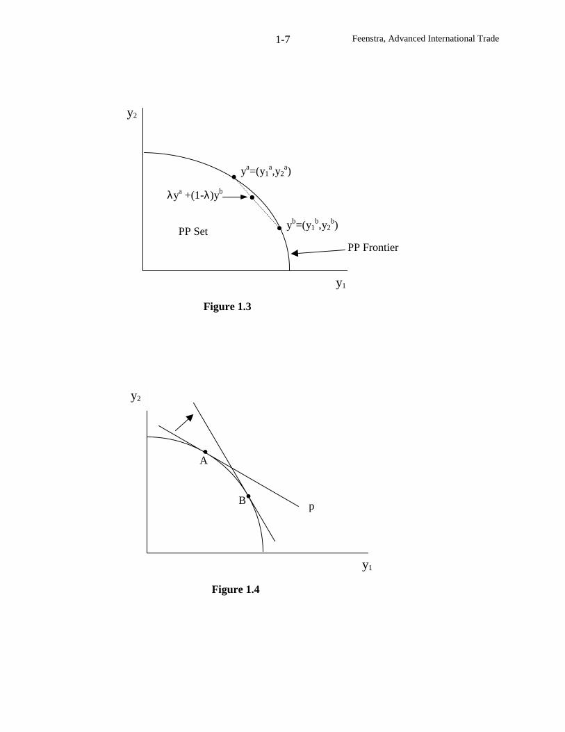
The production possibilities frontier summarizes the technology of the economy, but in
order to determine where the economy produces on the PPF we need to add some assumptions
about the market structure. We will assume perfect competition in the product markets and
factor markets. Furthermore, we will suppose that product prices are given exogenously: we
can think of these prices as established on world markets, and outside the control of the “small”
country being considered.
GDP Function
With the assumption of perfect competition, the amounts produced in each industry will
maximize gross domestic product (GDP) for the economy: this is Adam Smith’s “invisible
hand” in action. That is, the industry outputs of the competitive economy will be chosen to
maximize GDP:
)K,L,y(hy.t.sypypmax)K,L,p,p(G 122211y,y
2121
=+= . (1.2)
To solve this problem, we can substitute the constraint into the objective function and write it as
choosing y1 to maximize )K,L,y(hpyp 1211 + . The first-order condition for this problem is
,0)y/h(pp 121 =∂∂+ or,
1
2
12
1
y
y
y
h
p
pp
∂∂−=
∂∂−== . (1.3)
4 See problems 1.1 and 1.3 to prove the convexity of the production possibilities set, and to establish its slope.
Feenstra, Advanced International Trade1-9
Thus, the economy will produce where the relative price of good 1, p = p1/p2, is equal to the
slope of the production possbilities frontier.5 This is illustrated by the point A in Figure 1.4,
where the line tangent through point A has the slope of (negative) p. An increase in this price
will raise the slope of this line, leading to a new tangency at point B. As illustrated, then, the
economy will produce more of good 1 and less of good 2.
The GDP function introduced in (1.2) has many convenient properties, and we will make
use of it throughout this book. To show just one property, suppose that we differentiate the
GDP function with respect to the price of good i, obtaining:
∂∂+
∂∂+=
∂∂
i
12
i
11i
i p
yp
p
ypy
p
G. (1.4)
It turns out that the terms in parentheses on the right of (1.4) sum to zero, so that ii yp/G =∂∂ .
In other words, the derivative of the GDP function with respect to prices equals the outputs of
the economy. The fact that the terms in parentheses sum to zero is an application of the
“envelope theorem,” which states that when we differentiate a function that has been maximized
(such as GDP) with respect to an exogenous variable (such as pi), then we can ignore the
changes in the endogenous variables (y1 and y2) in this derivative. To prove that these terms
sum to zero, totally differentiate )K,L,y(hy 12 = with respect to y1 and y2 and use (1.3) to
obtain p1dy1= –p2dy2, or p1dy1 + p2dy2 = 0. This equality must hold for any small movement in
y1 and y2 around the PPF, and in particular, for the small movement in outputs induced by the
5 Notice the slope of the price line tangent to the PPF (in absolute value) equals the relative price of the good on thehorizontal axis, or good 1 in Figure 1.4.
Feenstra, Advanced International Trade1-10
change in pi. In other words, 0)p/y(p)p/y(p i22i11 =∂∂+∂∂ , so the terms in parentheses on the
right of (1.4) vanish and it follows that ii yp/G =∂∂ .6
Equilibrium Conditions
We now want to state succinctly the equilibrium conditions to determine factor prices and
outputs. It will be convenient to work with the unit-cost functions that are dual to the production
functions )K,L(f iii . These are defined by:
ci(w, r) =0K,L ii
min≥
{wLi + rKi | fi(Li, Ki) ≥ 1}. (1.5)
In words, ci(w,r) is the minimum cost to produce one unit of output. Because of our assumption
of constant returns to scale, these unit-costs are equal to both marginal costs and average costs.
It is easily demonstrated that the unit-cost functions ci(w, r) are non-decreasing and concave in
(w,r). We will write the solution to the minimization in (1.5) as ci(w, r) = waiL + raiK, where aiL
is optimal choice for Li, and aiK is optimal choice for Ki. It should be stressed that these optimal
choices for labor and capital depend on the factor prices, so that they should be written in full as
aiL(w, r) and aiK(w, r). However, we will usually not make these arguments explicit.
Differentiating the unit-cost function with respect to the wage, we obtain:
∂∂
+∂
∂+=
∂∂
w
ar
w
awa
w
c iKiLiL
i . (1.6)
6 Other convenient properties of the GDP function are explored in problem 1.4.
Feenstra, Advanced International Trade1-11
As we found with differentiating the GDP function, it turns out that the terms in parentheses on
the right of (1.6) sum to zero, which is again an application of the “envelope theorem.” It
follows that the derivative of the unit-costs with respect to the wage equals the labor needed for
one unit of production, iLi aw/c =∂∂ . Similarly, iKi ar/c =∂∂ .
To prove this result, notice that the constraint in the cost-minimization problem can be
written as the isoquant fi(aiL, aiK) = 1. Totally differentiate this to obtain ,0dafdaf iKiKiLiL =+
where iiiKiiiL K/ffandL/ff ∂∂≡∂∂≡ . This equality must hold for any small movement of
labor daiL and capital daiK around the isoquant, and in particular, for the change in labor and
capital induced by a change in wages. Therefore, 0)w/a(f)w/a(f iKiKiLiL =∂∂+∂∂ . Now
multiply this through by the product price pi, noting that pifiL = w and pifiK = r from the profit-
maximization conditions for a competitive firm. Then we see that the terms in parentheses on
the right of (1.6) sum to zero.
The first set of equilibrium conditions for the two-by-two economy is that profits equal
zero. This follows from free entry under perfect competition. The zero-profit conditions are
stated as:
.)r,w(cp
,)r,w(cp
22
11
==
(1.7)
The second set of equilibrium conditions is full-employment of both resources. These are
the same as the resource constraints (1.1), except that now we express them as equalities. In
addition, we will re-write the labor and capital used in each industry in terms of the derivatives
of the unit-cost function. Since iLi aw/c =∂∂ is the labor used for one unit of production, it
Feenstra, Advanced International Trade1-12
follows that the total labor used in Li = yi aiL , and similarly the total capital used is Ki = yi aiK.
Substituting these into (1.1), the full-employment conditions for the economy are written as:
.Kyaya
,Lyaya
21
21
K
2K2
K
1K1
L
2L2
L
1L1
=+
=+
321321
321321
(1.8)
Notice that (1.7) and (1.8) together are four equations in four unknowns, namely, (w, r)
and (y1, y2). The parameters of these equation, p1, p2, L and K, are given exogenously. Because
the unit-cost functions are nonlinear, however, it is not enough to just count equations and
unknowns: we need to study these equations in detail to understand whether the solutions are
unique and strictly positive, or not. Our task for the rest of this chapter will be to understand the
properties of these equations and their solutions.
To guide us in this investigation, there are three key questions that we can ask: (i) what
is the solution for factor prices; (ii) if prices change, how do factor prices change; (iii) if
endowments change, how do outputs change? Each of these questions are taken up in the
sections that follow. The methods we shall use follow the “dual” approach of Woodland (1977,
1982), Mussa (1979), and Dixit and Norman (1980).
Determination of Factor Prices
Notice that our four equation system above can be decomposed into the zero-profit
conditions as two equations in two unknowns – the wage and rental – and then the full-
empoyment conditions, which involve both the factor prices (which affect aiL and aiK) and the
outputs. It would be especially convenient if we could uniquely solve for the factor prices from
Feenstra, Advanced International Trade1-13
the zero-profit conditions, and then just substitute these into the full-employment conditions.
This will be possible when the hypotheses of the following Lemma, are satisfied:
Lemma (Factor Price Insensitivity)
So long as both goods are produced, and factor intensity reversals (FIR) do not occur, then each
price vector (p1, p2) corresponds to unique factor prices (w, r).
This is a remarkable result, because it says that the factor endowments )K,L( do not
matter for the determination of (w, r). We can contrast this result with a one-sector economy,
with production of )K,L(fy = , wages of Lpfw = , and diminishing marginal product fLL<0. In
this case, any increase in the labor endowments would certainly reduce wages, so that countries
with higher labor/capital endowments (L/K) would have lower wages. This is the result we
normally expect. In contrast, the above Lemma says that in a two-by-two economy, with a fixed
product price p, it is possible for the labor force or capital stock to grow without affecting their
factor prices! Thus, Leamer (1995) refers to this result as “factor price insensitivity.” Our goal
in this section is to prove the result and also develop the intuition for why it holds.
Two conditions must hold to obtain this result: first, that both goods are produced; and
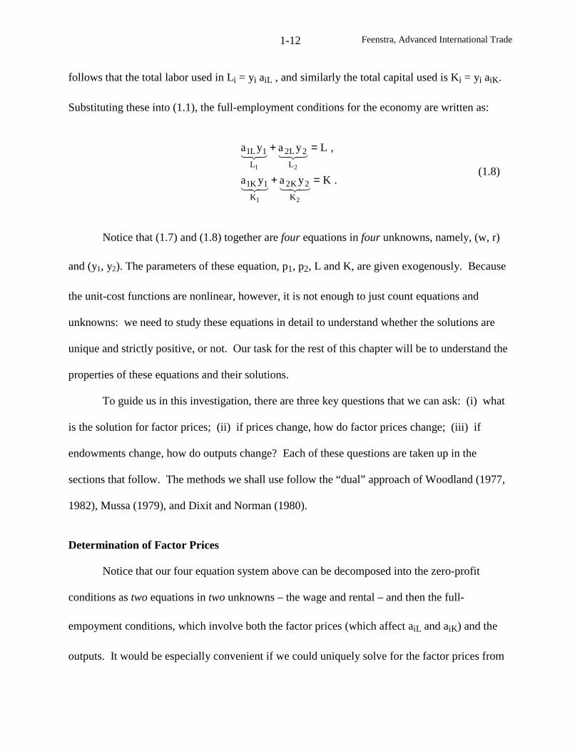
second, that factor intensity reversals (FIR) do not occur. To understand FIR, consider Figures
1.5 and 1.6. In the first case presented in Figure 1.5, we have graphed the two zero-profit
conditions, and the unit-cost lines intersect only once, at point A. This illustates the Lemma:
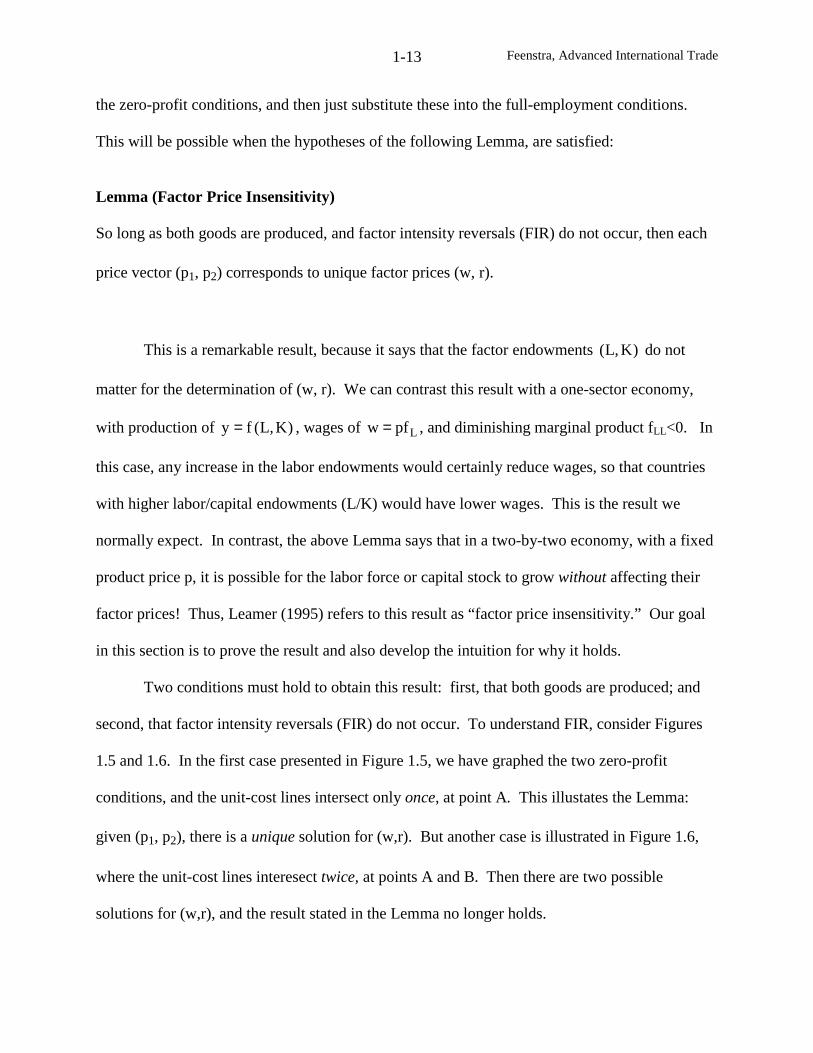
given (p1, p2), there is a unique solution for (w,r). But another case is illustrated in Figure 1.6,
where the unit-cost lines interesect twice, at points A and B. Then there are two possible
solutions for (w,r), and the result stated in the Lemma no longer holds.
Feenstra, Advanced International Trade1-14
p2=c2 (w, r)
p1=c1(w, r)
w
r
Figure 1.5
B
A
w
r
Figure 1.6
A
(a2L,a2K)
(a1L,a1K)
(b1L,b1K)
(b2L,b2K)
(a2L,a2K)
(a1L,a1K)
wB
wA
rB
rA
p1=c1(w, r)
p2=c2(w, r)
Feenstra, Advanced International Trade1-15
The case where the unit-cost lines intersect more than once corresponds to “factor
intensity reversals.” To see where this name comes from, let us compute the labor and capital
requirements in the two industries. We have already shown that aiL and aiK are the derivatives of
the unit-cost function with respect to factor prices, so it follows that the vectors (aiL, aiK) are the
gradient vectors to the iso-cost curves for the two industries in Figure 1.5. Recall from calculus
that gradient vectors point in the direction of the maximum increase of the function in question.
This means that they are orthogonal to their respective iso-cost curves, as shown by (a1L, a1K)
and (a2L, a2K) at point A. Each of these vectors has slope aiK/aiL, or the capital-labor ratio. It is
clear from Figure 1.5 that (a1L, a1K) has a smaller slope than (a2L, a2K), which means that
industry 2 is capital-intensive, or equivalently, industry 1 is labor-intensive. 7
In Figure 1.6, however, the situation is more complicated. Now there are two sets of
gradient vectors, which we label by (a1L, a1K) and (a2L, a2K) at point A and by (b1L, b1K) and
(b2L, b2K) at point B. A close inspection of the figure will reveal that industry 1 is labor-
intensive (a1K/a1L < a2K/a2L) at point A but is capital-intensive (b1K/b1L > b2K/b2L) at point B.
This illustrates a “factor intensity reversal”, whereby the comparison of factor intensities changes
at different factor prices.
While FIR might seem like a theoretical curiosum, they are actually quite realistic.
Consider the footwear industry, for example. While much of the footwear in the world is
7 Alternatively, we can totally differentiate the zero-profit conditions, holding prices fixed, to obtain 0 = aiLdw +
aiKdr. It follows that the slope of the iso-cost curve equals dr/dw = -aiL/aiK = -Li/Ki. Thus, the slope of each iso-cost curve equals the relative demand for the factor on the horizontal axis, whereas the slope of the gradient vector(which is orthogonal to the iso-cost curve) equals the relative demand for the factor on the vertical axis.
Feenstra, Advanced International Trade1-16
produced in developing nations, the United States retains a small number of plants. In sneakers,
New Balance has a plant in Norridgewock, Maine, where employers earn some $14 per hour.8
Some operate computerized equipment with up to 20 sewing machine heads running at once,
while others operate automated stitchers guided by cameras, that allow one person to do the work
of six. This is a far cry from the plants in Asia that produce shoes for Nike, Reebock and other
U.S. producers, using century-old technology and paying less than $1 per hour. The technology
used to make sneakers in Asia is like industry 1 at point A in Figure 1.5, using labor-intensive
technology and paying low wages wA
, while industry 1 in the U.S. is at point B, paying higher
wages wB
and using a capital-intensive technology.
As suggested by this discussion, when there are two possible solutions for the factor
prices such as points A and B in Figure 1.6, then some countries can be at one equilibrium and
others countries at the other. How do we know which country is where? To answer this, it is
necessary to consider the full-employment conditions: these will allow us to determine the factor
prices prevailing in each country. Notice that we have now re-introduced a link between factor
endowments (from the full-employment conditions) and factor prices, as we argued earlier in the
one-sector model: when there are FIR in the two-by-two model, it will turn out that a labor-
abundant country will be at an equilibrium like point A, paying low wages, while a capital-
abundant country will be at an equilibrium like point B, paying high wages.
To establish this link between factor endowments and prices, we need to graph the full-
employment conditions. We begin by re-writing these conditions in vector notation as:
8 The material that follows is drawn from Aaron Bernstein, “Low-Skilled Jobs: Do They Have to Move?”, BusinessWeek, February 26, 2001, pp. 94-95.
Feenstra, Advanced International Trade1-17
=
+
K
Ly
a
ay
a
a2
K2
L21
K1
L1 . (1.8’)
We have already illustrated the gradient vectors (aiL, aiK) to the iso-cost curves in Figures 1.5
and 1.6. Now let us take these vectors and re-graph them, in Figures 1.7 and 1.8. In the simpler
case of Figure 1.7, we have a single equilibrium for factor prices and a single set of labor and
capital requirements (a1L, a1K) and (a2L, a2K). Multiplying each of these by the output of their
respective industries, we obtain the total labor and capital demands y1(a1L, a1K) and y2(a2L, a2K).
Summing these as in (1.8’) we obtain the labor and capital endowments )K,L( . But this
exercise can also be performed in reverse: for any endowment vector )K,L( , there will be a
unique value for the outputs (y1, y2) such that when (a1L, a1K) and (a2L, a2K) are multiplied by
these amounts, they will sum to the endowments.
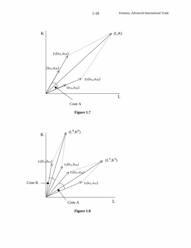
How can we be sure that the outputs obtained from (1.8’) are positive? It is clear from
Figure 1.7 that the outputs in both industries will be positive if and only if the endowment vector
)K,L( lies in-between the factor requirement vectors (a1L, a1K) and (a2L, a2K). For this reason,
the space spanned by these two vectors is called a “cone of diversification”, which we label by
cone A in Figure 1.7. In contrast, if the endowment vector )K,L( lies outside of this cone, then
it is impossible to add together any positive multiples of the vectors (a1L, a1K) and (a2L, a2K) and
arrive at the endowment vector. So if )K,L( lies outside of the cone of diversification, then it
must be that only one good is produced. At the end of the chapter, we will show how to
determine which good it is.9 For now, we should just recognize that when only one good is
9 See problem 1.5.
Feenstra, Advanced International Trade1-18
L
K
Figure 1.8
K
L
Cone A
Figure 1.7
y2(a2L,a2K)
y1(a1L,a1K)
(a1L,a1K)
(a2L,a2K)
y1(a1L,a1K)
y2(b2L,b2K)y1(b1L,b1K)
Cone B
Cone A
(LA,KA)
(LB,KB)
y2(a2L,a2K)
(L,K)
Feenstra, Advanced International Trade1-19
produced, then factor prices are determined by the marginal products of labor and capital as in
the one-sector model, and will certainly depend on the factor endowments. This is why the
Lemma stated above requires that both goods are produced, or equivalently, that the
endowments are inside the “cone of diversification.”
Now consider the more complex case in Figure 1.8, where we have re-drawn the two sets
of gradient vectors (a1L, a1K) and (a2L, a2K), and (b1L, b1K) and (b2L, b2K) from Figure 1.6, after
multiplying each of them by the outputs of their respective industries. These vectors create two
cones of diversification, labeled as cone A and cone B. Now we can answer the question of
which factor prices will apply in any given country: a labor abundant economy, with a high
ratio of labor/capital endowments such as )K,L( AA in cone A of Figure 1.8, will have factor
prices given by (wA
, rA
) in Figure 1.6, with low wages; whereas a capital abundant economy
with a high ratio of capital/labor endowments such as shown by )K,L( BB in cone B, will have
factor prices given by (wB
, rB
), with high wages. Thus, factor prices will depend on the
endowments of the economy. A labor-abundant country such as China will pay low wages and a
high rental (as in cone A). In contrast, a capital-abundant country such as the United States will
have high wages and a low rental (as in cone B).
In summary, the “single cone” illustrated in Figures 1.5 and 1.7 show how we solve the
zero-profit conditions (1.7) when there is a unique solution for the factor prices, and then use this
solution in the full-employment conditions (1.8) to evaluate the aij coefficients and solve for
outputs. In comparison, the “multi-cone” as presented in Figures 1.6and 1.8 show that when
there are multiple solutions for factor prices from the zero-profit conditions, then we also need to
make use of the full-employment conditions to determine which factor prices prevail in each
Feenstra, Advanced International Trade1-20
country. Despite the complexity of the latter case, many trade economists feel that countries do
in fact produce in different cones of diversification, and taking this possibility into account is a
topic of current research.10
Let us conclude this section by returning to the simple case of a single cone of
diversification, in which the Lemma stated above applies. What are the implications of this
result for the determination of factor prices under free trade? To answer this question, let us
sketch out some of the assumptions of the Heckscher-Ohlin model, which we be study in more
details in the next chapter. We assume that there are two countries, with identical technologies
but different factor endowments. We continue to assume that labor and capital are the two
factors of production, so that under free trade the equilibrium conditions (1.7) and (1.8) apply in
each country with the same product prices (p1,p2). With a single cone of diversification, we can
draw Figures 1.5 and 1.7 for each country. Allowing factor endowments to differ across the
countries will not affect the factor prices provided that both countries stay within the cone of
diversification. In other words, the wage and rental determined by Figure 1.7 is identical in the
two countries. We have therefore proved the Factor Price Equalization Theorem, which is stated
as follows:
Factor Price Equalization Theorem (Samuelson, 1949)
Suppose that two countries are engaged in free trade, having identical technologies but different
factor endowments. If both countries are diversified and FIR do not occur, then the factor prices
(w, r) are equalized across these countries.
10 Empirical evidence on whether developed countries fit into the same cone is presented by deBaere andDemiroglu (2000), and the presence of multiple cones is explored by Leamer (1987), Harrigan and Zakrajšek(2000), Schott (2000) and Xu (2002). The latter papers draw on empirical methods that we introduce in chapter 3.
Feenstra, Advanced International Trade1-21
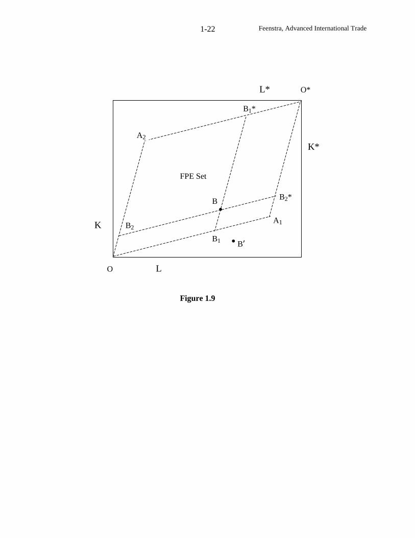
To illustrate this result, we engage in a thought experiment posed by Samuelson (1949)
and further developed by Dixit and Norman (1980). Initially, suppose that labor and capital are
free to move between the two countries until their factor prices are equalized. Then all that
matters for factor prices are the world endowments of labor and capital, and these are shown as
the length of the horizontal and vertical axis in Figure 1.9. The amounts of labor and capital
choosing to reside at home are measured relative to the origin 0, while the amounts choosing to
reside in the foreign country are measured relative to the origin 0* – suppose that this allocation
is at point B. Given the world endowments we establish equilibrium prices for goods and factors
in this “integrated world equilibrium.” The factor prices determine the demand for labor and
capital in each industry, and using these, we can construct the diversification cone (since factor
prices are the same across countries, then the diversification cone is also the same). Let us plot
the diversification cone relative to the home origin 0, and again relative to the foreign origin 0*.
These cones form the parallelogram 0A10*A2.
For later purposes, it is useful to identify precisely the points A1 and A2, on the vertexes
of this parallelogram. The vectors 0Ai and 0*Ai are proportional to (aiL,aiK), the amount of labor
and capital used to produce one unit of good i in each country. Multiplying (aiL,aiK) by world
demand for good i, wiD , we then obtain the total labor and capital used to produce that good, so
that Ai = (aiL,aiK) wiD . Summing these gives the total labor and capital used in world demand,
which equals the labor and capital used in world production, or world endowments.
Feenstra, Advanced International Trade1-22
O L
K
K*
L* O*
Figure 1.9
A1
A2
FPE Set
B1
B2
B1*
B2*B
B’
Feenstra, Advanced International Trade1-23
Now we ask whether we can achieve exactly the same world production and equilibrium
prices as in this “integrated world equilibrium,” but without labor and capital mobility. Suppose
there is some allocation of labor and capital endowments across the countries, such as point B.
Then can we produce the same amount of each good as in the “integrated world equilibrium”?
The answer is clearly yes: with labor and capital in each country at point B, we could devote
0B1 of resources to good 1 and 0B2 to good 2 at home, while devoting 0*B1* to good 1 and
0*B2* towards good 2 abroad. This will ensure that the same amount of labor and capital
worldwide is devoted to each good as in the “integrated world equilibrium”, so that production
and equilibrium prices must be the same as before. Thus, we have achieved the same
equilibrium but without factor mobility. It will become clear in the next chapter that there is still
trade in goods going on to satisfy the demands in each country.
More generally, for any allocation of labor and capital within the parallelogram 0A10*A2
both countries remain diversified (producing both goods), and we can achieve the same
equilibrium prices as in the “integrated world economy.” It follows that factor prices remain
equalized across countries for allocations of labor and capital within the parallelogram 0A10*A2,
which is referred to as the Factor Price Equalization (FPE) set. The FPE set illustrates the range
of labor and capital endowments between countries for which factor price equalization is
obtained. In contrast, for endowments outside of the FPE set such as point B’, then at least one
country would have to be fully specialized in one good and FPE no longer holds.
The FPE theorem is a remarkable result because it says that trade in goods has the ability
to equalize factor prices: in this sense, trade in goods is a “perfect substitute” for trade in factors.
We can again contrast this result with that obtained from a one-sector economy in both countries.
In that case, equalization of the product price through trade would certainly not equalize factor
Feenstra, Advanced International Trade1-24
prices: the labor abundant country would be paying a lower wage. Why does this outcome not
occur when there are two sectors? The answer is that the labor abundant country can produce
more of, and export, the labor-intensive good. In that way it can fully employ its labor while still
paying the same wages as a capital abundant country. In the two-by-two model, the opportunity
to disproportionately produce more of one good than the other, while exporting the amounts not
consumed at home, is what allows factor price equalization to occur. This intuition will become
even clearer as we continue to study the Heckscher-Ohlin model in the next chapter.
Change in Product Prices
Let us move on now to the second of our key questions of the two-by-two model: if the
product prices change, how will the factor prices change? To answer this, we perform
comparative statics on the zero-profits conditions (1.7). Totally differentiating these conditions,
we obtain:
dradwadp iKiLi += ⇒r
dr
c
ra
w
dw
c
wa
p
dp
i
iK
i
iL
i
i += , i=1,2. (1.9)
The second equation is obtained by multiplying and dividing like terms, and noting that
pi = ci(w,r). The advantage of this approach is that it allows us to express the variables in terms
of percentage changes, such as w/dwwlnd = , as well as cost shares. Specifically, let
θiL = waiL/ci denote the cost share of labor in industry i, while θiK = raiK/ci denotes the cost share
of capital. The fact that costs equal ci = waiL + raiK ensures that the shares sum to unity,
iLθ + iKθ =1. In addition, denote the percentage changes by rr/drandww/dw == . Then
(1.9) can be re-written as:
rwp iKiLi θ+θ= , i=1,2. (1.9’)
Feenstra, Advanced International Trade1-25
Expressing the equation using these cost shares and percentage changes follows Jones (1965),
and is referred to as the “Jones’ algebra.” This system of equation can be written in matrix form
and solved as:
θθ−θ−θ
θ=
⇒
θθθθ
=
2
1
L1L2
K1K2
K2L2
K1L1
2
1
p
p1r
w
r
w
p
p, (1.10)
where θ denotes the determinant of the 2x2 matrix on the left. This determinant can be
expressed as:
K1K2L2L1
L2L1L2L1
L2K1K2L1
)1()1(
θ−θ=θ−θ=θθ−−θ−θ=
θθ−θθ=θ(1.11)
where we have repeatedly made use of the fact that iLθ + iKθ =1.
In order to fix ideas, let us assume henceforth that industry 1 is labor intensive. This
implies that the cost share in industry 1 exceeds that in industry 2, L1θ – L2θ > 0, so that θ >0 in
(1.11).11 Furthermore, suppose that the relative price of good 1 increases, so that
0ppp 21 >−= . Then we can solve for the change in factor prices from (1.10) and (1.11) as:
1K1K2
21K11K1K22K11K2 p)(
)pp(p)(ppw >
θ−θ−θ+θ−θ=
θθ−θ= , since 0pp 21 >− , (1.12a)
and, 2L2L1
21L22L2L11L22L1 p)(
)pp(p)(ppr <
θ−θ−θ−θ−θ=
θθ−θ= , since 0pp 21 >− . (1.12b)
11 As an exercise, show that 1K/1L > 2K/2L ⇔ L2L1 θ>θ . This is done by multipying the numerator and
denominator on both sides of the first inequality by like terms, so as to convert it into cost shares.
Feenstra, Advanced International Trade1-26
From the result in (1.12a), we see that the wage increases by more than the price of good
1, 21 ppw >> . This means that workers can afford to buy more of good 1 (w/p1 has gone up),
as well as more of good 2 (w/p2 has gone up). When labor can buy more of both goods in this
fashion, we say that the real wage has increased. Looking at the rental on capital in (1.12b), we
see that the rental r changes by less than the price of good 2. It follows that capital-owner can
afford less of good 2 (r/p2 has gone down), and also less of good 1 (r/p1 has gone down). Thus
the real return to capital has fallen. We can summarize these results with the following:
Stolper-Samuelson (1941) Theorem
An increase in the relative price of a good will increase the real return to the factor used
intensively in that good, and reduce the real return to the other factor.
To develop the intuition for this result, let us go back to the differentiated zero-profit
conditions in (1.9’). Since the cost shares add up to unity in each industry, we see from equation
(1.9’) that ip is a weighted average of the factor price changes w and r . This implies that ip
necessarily lies in-between w and r . Putting these together with our assumption that
0pp 21 >− , it is therefore clear that:
rppw 21 >>> . (1.13)
Jones (1965) has called this set of inequalities the “magnification effect”: they show that any
change in the product price has a magnified effect on the factor prices. This is an extremely
important result. Whether we think of the product price change is due to export opportunities for
a country (the export price goes up), or due to lowering import tariffs (so the import price goes
Feenstra, Advanced International Trade1-27
down), the magnification effect says that there will be both gainers and losers due to this change.
Even though we will argue in chapter 6 that there are gains from trade in some overall sense, it is
still the case that trade opportunities have strong distributional consequences, making some
people worse off and some better off!
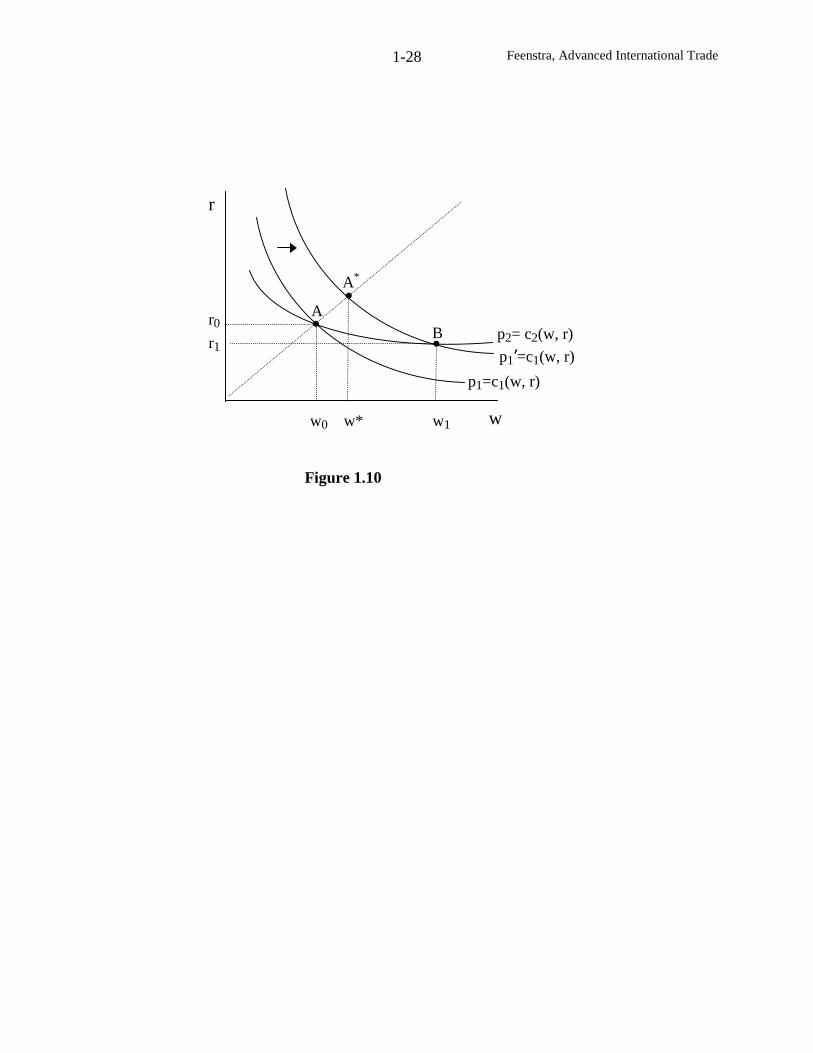
We conclude this section by illustrating the Stolper-Samuelson Theorem in Figure 1.10.
We begin with an initial factor price equilibrium given by point A, where industry 1 is labor-
intensive. An increase in the price of that industry will shift out the iso-cost curve, and as
illustrated, move the equilibrium to point B. It is clear that the wage has gone up, from w0 to w1,
and the rental has declined, from r0 to r1. Can we be sure that the wage has increased in
percentage terms by more than the relative price of good 1? The answer is yes, as can be seen by
drawing a ray from the origin through the point A. Because the unit-cost functions are
homogeneous of degree one in factor prices, moving along this ray increases p and (w,r) in the
same proportion. Thus, at the point A*, the increase in the wage exactly matched the percentage
change in the price p. But it is clear that the equilibrium wage increases by more, w1 > w*, so
the percentage increase in the wage exceeds that of the product price, which is the Stolper-
Samuelson result.
Changes in Endowments
We turn now to the third key question: if endowments change, how do the industry
outputs change? To answer this, we hold the product prices fixed and totally differentiate the
full-employment conditions (1.8) to obtain:
Feenstra, Advanced International Trade1-28
A*
BA
r
r0
r1
w0 w* w1 w
p1=c1(w, r)
p2= c2(w, r)
Figure 1.10
p1’=c1(w, r)
Feenstra, Advanced International Trade1-29
.dKdyadya
,dLdyadya
2K21K1
2L21L1
=+=+
(1.14)
Notice that the aij coefficients do not change, despite the fact that they are functions of the factor
prices (w, r). These coefficients are fixed because p does not change, so from our earlier
Lemma, the factor prices are also fixed.
By re-writing the equations in (1.14) using the “Jone’s algebra”, we obtain:
K
dK
y
dy
K
ay
y
dy
K
ay
L
dL
y
dy
L
ay
y
dy
L
ay
2
2K22
1
1K11
2
2L22
1
1L11
=+
=+
Kyy
Lyy
2K21K1
2L21L1
=λ+λ
=λ+λ⇒. (1.14’)
To move from the first set of equations to the second, we denote the percentage changes
11 y/dy = 1y , and likewise for all the other variables. In addition, we define )L/ay( iLiiL ≡λ
)L/L( i= , which measures the fraction of the labor force employed in industry i, where
1L2L1 =λ+λ . We define iKλ analogously as the fraction of the capital stock employed in
industry i.
This system of equations is written in matrix form and solved as:
=
λλλλ
K
L
y
y
2
1
K2K1
L2L1
λλ−λ−λ
λ=
⇒
K
L1
y
y
L1K1
L2K2
2
1 , (1.15)
where λ denotes the determinant of the 2x2 matrix on the left, which is simplified as:
L2K2K1L1
K1L1K1L1
K1L2K2L1
)1()1(
λ−λ=λ−λ=λλ−−λ−λ=
λλ−λλ=λ(1.16)
Feenstra, Advanced International Trade1-30
where we have repeatedly made use of the fact that 1L2L1 =λ+λ and 1K2K1 =λ+λ .
Recall that we assumed industry 1 to be labor-intensive. This implies that the share of
the labor force employed in industry 1 exceeds the share of the capital stock used there,
0K1L1 >λ−λ , so that λ >0 in (1.16).12 Suppose further that the endowments of labor is
increasing, while the endowments of capital remains fixed such that .0Kand,0L => Then we
can solve for the change in outputs from (1.15)-(1.16) as,
0yand0LL)(
y K12
L2K2
K21 <
λλ
=>>λ−λ
λ= . (1.17)
From (1.17), we see that the output of the labor-intensive industry 1 expands, whereas the output
of industry 2 contracts. We have therefore established:
Rybczynski (1955) Theorem:
An increase in a factor endowment will increase output of the industry using it intensively, and
decrease the output of the other industry.
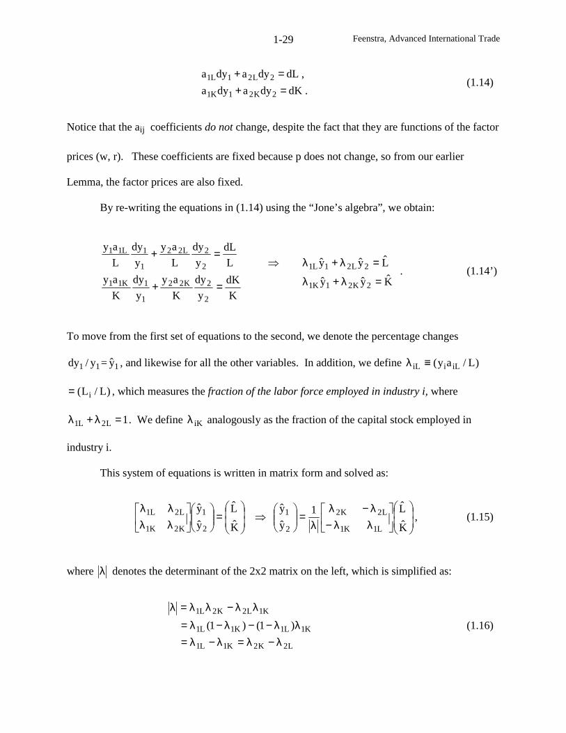
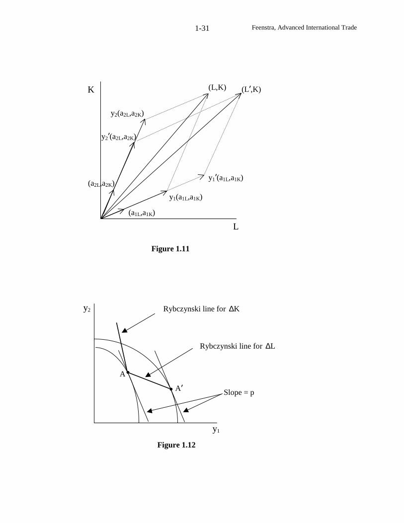
The intitution for this result is developed in Figure 1.11. With the initial endowments
)K,L( , the equilibrium outputs are y1 and y2. Now suppose that the labor endowment increases
to L’ > L, with no change in the capital endowment. Starting from the endowments (L’,K), the
only way to add up multiples of (a1L, a1K) and (a2L, a2K) and obtain the endowments is to
12 As an exercise, show that 1K/1L > K/L > 2K/2L ⇔ K1L1 λ>λ and L2K2 λ>λ . This is done by multipying
the numerator and denominator in the first set of inequalities by like terms.
Feenstra, Advanced International Trade1-31
Figure 1.11
K
(a1L,a1K)
(a2L,a2K)
L
Slope = p
Rybczynski line for L∆
Rybczynski line for K∆y2
Figure 1.12
A
A’
y1
(L,K) (L’,K)
y1(a1L,a1K)
y2’(a2L,a2K)
y2(a2L,a2K)
y1’(a1L,a1K)
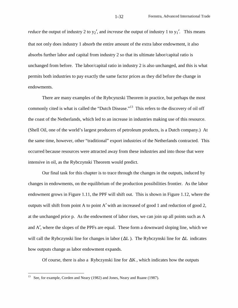
Feenstra, Advanced International Trade1-32
reduce the output of industry 2 to y2’, and increase the output of industry 1 to y1’. This means
that not only does industry 1 absorb the entire amount of the extra labor endowment, it also
absorbs further labor and capital from industry 2 so that its ultimate labor/capital ratio is
unchanged from before. The labor/capital ratio in industry 2 is also unchanged, and this is what
permits both industries to pay exactly the same factor prices as they did before the change in
endowments.
There are many examples of the Rybcynzski Theorem in practice, but perhaps the most
commonly cited is what is called the “Dutch Disease.”13 This refers to the discovery of oil off
the coast of the Netherlands, which led to an increase in industries making use of this resource.
(Shell Oil, one of the world’s largest producers of petroleum products, is a Dutch company.) At
the same time, however, other “traditional” export industries of the Netherlands contracted. This
occurred because resources were attracted away from these industries and into those that were
intensive in oil, as the Rybczynski Theorem would predict.
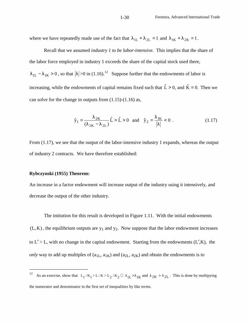
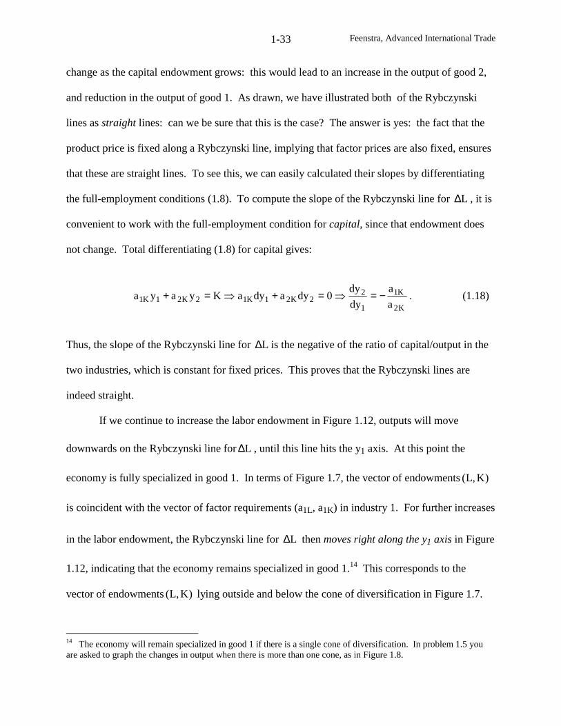
Our final task for this chapter is to trace through the changes in the outputs, induced by
changes in endowments, on the equilibrium of the production possibilities frontier. As the labor
endowment grows in Figure 1.11, the PPF will shift out. This is shown in Figure 1.12, where the
outputs will shift from point A to point A’ with an increased of good 1 and reduction of good 2,
at the unchanged price p. As the endowment of labor rises, we can join up all points such as A
and A’, where the slopes of the PPFs are equal. These form a downward sloping line, which we
will call the Rybczynski line for changes in labor ( L∆ ). The Rybczynski line for L∆ indicates
how outputs change as labor endowment expands.
Of course, there is also a Rybczynski line for K∆ , which indicates how the outputs
13 See, for example, Corden and Neary (1982) and Jones, Neary and Ruane (1987).
Feenstra, Advanced International Trade1-33
change as the capital endowment grows: this would lead to an increase in the output of good 2,
and reduction in the output of good 1. As drawn, we have illustrated both of the Rybczynski
lines as straight lines: can we be sure that this is the case? The answer is yes: the fact that the
product price is fixed along a Rybczynski line, implying that factor prices are also fixed, ensures
that these are straight lines. To see this, we can easily calculated their slopes by differentiating
the full-employment conditions (1.8). To compute the slope of the Rybczynski line for L∆ , it is
convenient to work with the full-employment condition for capital, since that endowment does
not change. Total differentiating (1.8) for capital gives:
K2
K1
1
22K21K12K21K1 a
a
dy
dy0dyadyaKyaya −=⇒=+⇒=+ . (1.18)
Thus, the slope of the Rybczynski line for L∆ is the negative of the ratio of capital/output in the
two industries, which is constant for fixed prices. This proves that the Rybczynski lines are
indeed straight.
If we continue to increase the labor endowment in Figure 1.12, outputs will move
downwards on the Rybczynski line for L∆ , until this line hits the y1 axis. At this point the
economy is fully specialized in good 1. In terms of Figure 1.7, the vector of endowments )K,L(
is coincident with the vector of factor requirements (a1L, a1K) in industry 1. For further increases
in the labor endowment, the Rybczynski line for L∆ then moves right along the y1 axis in Figure
1.12, indicating that the economy remains specialized in good 1.14 This corresponds to the
vector of endowments )K,L( lying outside and below the cone of diversification in Figure 1.7.
14 The economy will remain specialized in good 1 if there is a single cone of diversification. In problem 1.5 youare asked to graph the changes in output when there is more than one cone, as in Figure 1.8.
Feenstra, Advanced International Trade1-34
With the economy fully specialized in good 1, factor prices are determined by the marginal
products of labor and capital in that good, and the earlier “factor price insensitivity” Lemma no
longer applies.
Conclusions
In this chapter we have reviewed several two-sector models: the Ricardian model, with
just one factor, and the two-by-two model, with two factors both of which are fully mobile
between industries. There are other two-sector models, of course: if we add a third factor,
treating capital as specific to each sector but labor as mobile, then we obtain the Ricardo-Viner
or “sector-specific” model, as will be discussed in chapter 3. We will have an opportunity to
make use of the two-by-two model throughout this book, and a thorough understanding of its
properties, as presented in this chapter, is essential for all the material that follows.
This is the only chapter where we do not present any accompanying empirical evidence.
The reader should not infer from this that the two-by-two model is unrealistic: while it is usually
necessary to add more goods or factors to this model before confronting it with data, the
relationships between prices, outputs and endowments that we have identified in this chapter will
carry over in some form to more general settings. Evidence on the pattern of trade is presented
in the next chapter, where we extend the two-by-two model by adding another country, and then
many countries, trading with each other. We also allow for many goods and factors, but for the
most part restrict attention to situations where factor price equalization holds. In chapter 3, we
examine the case of many goods and factors in greater detail, to determine whether the Stolper-
Samuelson and Rybczynski Theorems generalize and also how to estimate these effects. In
chapter 4, evidence on the relationship between product prices and wages is examined in detail,
using a model that allows for trade in intermediate inputs. The reader is already well prepared
Feenstra, Advanced International Trade1-35
for these chapters that follow, based on the tools and intuition we have developed from the two-
by-two model. Before moving on, you are encouraged to complete the problems at the end of
this chapter.
Feenstra, Advanced International Trade1-36
Problems
1.1 Rewrite the production function y1 = f1(L1,K1) as y1 = f1(v1), and similarly, y2 = f2(v2).
Concavity means that given two points )v(fy a11
a1 = and )v(fy b
11b1 = , and 0 < λ < 1, then
b1
a1
b1
a11 y)1(y)v)1(v(f λ−+λ≥λ−+λ . Similarly for the production function y2 = f2(v2).
Consider two points )y,y(y a2
a1
a = and )y,y(y b2
b1
b = , both of which can be produced while
satisfying the full-employment conditions Vvv a2
a1 ≤+ and Vvv b
2b1 ≤+ , where V are the
endowments. Consider a production point mid-way between these, ba y)1(y λ−+λ . Then use
the concavity of the production functions to show that this point can also be produced while
satisfying the full-employment conditions. This proves that the production possibilities set is
convex. (Hint: Rather than showing that ba y)1(y λ−+λ can be produced while satisfying the
full-employment conditions, consider instead allocating b1
a1 v)1(v λ−+λ of the resources to
industry 1, and b2
a2 v)1(v λ−+λ of the resources to industry 2. )
1.2 Any function y = f(v) is homogeneous of degree α if for all λ>0, f(λv) = λα f(v).
Differentiating with respect to α and evaluating at α=1, we therefore obtain: )v(fv)'v(fv α= .
Consider the production function y=f(L,K), which we assume is homogeneous of degree one, so
that f(λL,λK) = λf(L,K). Now differentiate this expression with respect to L, and answer:
Is the marginal product fL(L,K) homogeneous, and of what degree? Use the expression you have
obtained to show that fL(L/K,1) = fL(L,K).
Feenstra, Advanced International Trade1-37
1.3 Consider the problem of maximizing y1 = f1(L1,K1), subject to the full-employment
conditions L1+L2 < L and K1+K2 < K, and the constraint y2 = f2(L2,K2). Set this up as a
Lagrangian, and obtain the first-order conditions. Then use the Lagrangian to solve for dy1/dy2,
which is the slope of the production possibilities frontier. How is this slope related to the
marginal product of labor and capital?
1.4 Consider the problem of maximizing p1f1(L1,K1)+ p2f2(L2,K2), subject to the full-
employment constraints L1+L2 < L and K1+K2 < K. Call the result the GDP function G(p,L,K),
where p = (p1,p2) is the price vector. Then answer:
(a) What is ∂G/∂pi? (Hint: we solved for this in the chapter)
(b) Give an economic interpretation to ∂G/∂L and ∂G/∂K.
(c) Give an economic interpretation to ∂2G/∂pi∂L = ∂2
G/∂L∂pi, and ∂2G/∂pi∂K = ∂2
G/∂K∂pi .
1.5 Trace through changes in outputs when there are factor intensity reversals. That is,
construct a graph with the capital endowment on the horizontal axis, and the output of good 1 on
the vertical axis. Starting at a point of diversification (where both goods are produced) in cone A
of Figure 1.8, draw the changes in output of good 1 as the capital endowment grows outside of
cone A, into cone B, and beyond this.
Feenstra, Advanced International Trade
Chapter 2: The Heckscher-Ohlin Model
We begin this chapter by describing the Heckscher-Ohlin model with two countries, two
goods, and two factors (or the 2x2x2 model). This formulation is often called the Heckscher-
Ohlin-Samuelson (HOS) model, based on the work of Paul Samuelson who developed a
mathematical model from the original insights of Eli Heckscher and Bertil Ohlin.1 The goal of
that model is to predict the pattern of trade in goods between the two countries, based on their
differences in factor endowments. Following this, we present the multi-good, multi-factor
extension that is associated with the work of Vanek (1968), and is often called the Heckscher-
Ohlin-Vanek (HOV) model. As we shall see, in this latter formulation we do not attempt to keep
track of the trade pattern in individual goods, but instead, compute the “factor content” of trade,
i.e. the amounts of labor, capital, land, etc. embodied in the exports and imports of a country.
The factor-content formulation of the HOV model has led to a great deal of empirical
research, beginning with Leontief (1953) and continuing with Leamer (1980), Bowen, Leamer
and Sveikauskas (1987), Trefler (1993, 1995), Davis and Weinstein (2001a), with many other
writers in-between. We will explain the twists and turns in this chain of empirical research. The
bottom line is that the HOV model performs quite poorly empirically unless we are willing to
dispense with the assumption of identical technologies across countries. This brings us back to
the earlier tradition of the Ricardian model of allowing for technological differences, which also
implies differences in factor prices across countries. We will show several ways that
technological differences can be incorporated into an “extended” HO model, and their empirical
results, and this remains a question of ongoing research.
1 The original 1919 article of Heckscher and the 1924 dissertation of Ohlin have been translated from Swedish andedited by Harry Flam and June Flanders, and published as Heckscher and Ohlin (1991).
Feenstra, Advanced International Trade2-2
Heckscher-Ohlin-Samuelson (HOS) model
The basic assumptions of the HOS model were already introduced in the previous
chapter: identical technologies across countries; identical and homothetic tastes across countries;
differing factor endowments; and free trade in goods (but not factors). For the most part, we will
also assume away the possibility of factor-intensity reversals. Provided that all countries have
their endowments within their “cone of diversification,” this means that factor prices are
equalized across countries
We begin by supposing that there are just two countries, two sectors and two factors,
exactly like the two-by-two model we introduced in chapter 1. We shall assume that the home
country is labor abundant, so that *K/*LK/L > . We will also assume that good 1 is labor
intensive. The countries engage in free trade, and we also suppose that trade is balanced (value
of exports = value of imports). Then the question is: what is the pattern of trade in goods
between the countries? This is answered by:
Heckscher-Ohlin Theorem
Each country will export the good that uses its abundant factor intensively.
Thus, under our assumptions the home country will export good 1 and the foreign
country will export good 2. To prove this, let us take a particular case of the factor endowment
differences *K/*LK/L > , and assume that the labor endowments are identical in the two
countries, L* = L, while the foreign capital endowments exceeds that at home, K*K > .2 In
order to derive the pattern of trade between the countries, we proceed by first establishing what
2 Because of the assumptions of identical homothetic tastes and constant returns to scale, the result we areestablishing remains valid if the labor endowments also differ across countries.
Feenstra, Advanced International Trade2-3
the relative product price is in each country without any trade, or in autarky. As we shall see, the
pattern of autarky prices can then be used to predict the pattern of trade: a country will export
the good whose free trade price is higher than its autarky price, and import the other.
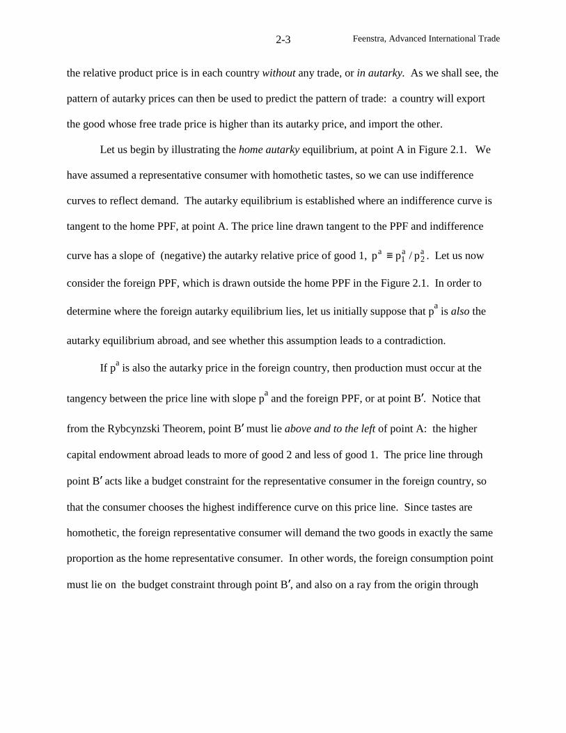
Let us begin by illustrating the home autarky equilibrium, at point A in Figure 2.1. We
have assumed a representative consumer with homothetic tastes, so we can use indifference
curves to reflect demand. The autarky equilibrium is established where an indifference curve is
tangent to the home PPF, at point A. The price line drawn tangent to the PPF and indifference
curve has a slope of (negative) the autarky relative price of good 1, a2
a1
a p/pp ≡ . Let us now
consider the foreign PPF, which is drawn outside the home PPF in the Figure 2.1. In order to
determine where the foreign autarky equilibrium lies, let us initially suppose that pa
is also the
autarky equilibrium abroad, and see whether this assumption leads to a contradiction.
If pa is also the autarky price in the foreign country, then production must occur at the
tangency between the price line with slope pa
and the foreign PPF, or at point B’. Notice that
from the Rybcynzski Theorem, point B’ must lie above and to the left of point A: the higher
capital endowment abroad leads to more of good 2 and less of good 1. The price line through
point B’ acts like a budget constraint for the representative consumer in the foreign country, so
that the consumer chooses the highest indifference curve on this price line. Since tastes are
homothetic, the foreign representative consumer will demand the two goods in exactly the same
proportion as the home representative consumer. In other words, the foreign consumption point
must lie on the budget constraint through point B’, and also on a ray from the origin through
Feenstra, Advanced International Trade2-4
A
C’
B’
y2
y1
pa
Figure 2.1
AA*
y1
y2
C
B
*1y
*2y
C*
B*
Figure 2.2(a): Home Country Figure 2.2(b): Foreign Country
Feenstra, Advanced International Trade2-5
point A. Thus, foreign consumption must occur at point C’, which is above and to the right of
point A. Since points B’ and C’ do not coincide, we have arrived at a contradiction: the relative
price pa
at home cannot equal the autarky price abroad, and on the contrary, at this price there is
an excess demand for good 1 in the foreign country. This excess demand will bid up the relative
price of good 1, so that the foreign autarky price must be higher than at home, ∗ap > pa.
To establish the free trade equilibrium price, let z(p) denote the excess demand for good 1
at any prevailing price p at home, while z*(p*) denotes the excess demand for good 1 abroad.
World excess demand at a common price is therefore z(p) + z*(p*), and a free trade equilibrium
occurs when world excess demand is equal to zero. The home autarky equilibrium satisfies
z(pa) = 0, and we have shown above that z*(p
a) > 0. It follows that z(p
a) + z*(p
a) > 0. If instead
we reversed the argument in Figure 2.1, and started with the foreign autarky price satisfying
z*( ∗ap ) = 0, then we could readily prove that z( ∗ap ) < 0, so at the foreign autarky price there is
excess supply of good 1 at home. It follows that world excess demand would satisfy z( ∗ap ) +
z*( ∗ap ) < 0. Then by continuity of the excess demand functions, there must be a price p, with
∗ap > p > pa, such that z(p) + z*(p) = 0. This is the equilibrium price with free trade.
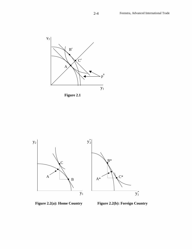
Let us illustrate the free trade equilibrium, in Figure 2.2. In panel (a) we show the
equilibrium at home, and in panel (b) we show the equilibrium in the foreign country. Beginning
at the home autarky point A, the relative price of good 1 rises at home, p > pa. It follows that
production will occur at a point like B, where the price line through point B has the slope p.
Once again, this price line acts as a budget constraint for the representative consumer, and utility
is maximized at point C. The difference between production at point B and consumption at point
Feenstra, Advanced International Trade2-6
C is made up through exporting good 1 and importing good 2, as illustrated by the “trade
triangle” drawn. This trade pattern at home establishes the HO Theorem stated above. In the
foreign country, the reverse pattern occurs: the relative price of good 1 falls, ∗ap > p, production
moves from the autarky equilibrium point A* to production at point B* and consumption at point
C*, where good 1 is imported and good 2 is exported. Notice that the trade triangles drawn at
home and abroad are identical in size: the exports of one country must be imports of the other.3
In addition to establishing the trade pattern, the HO model has precise implications about
who gains and who loses from trade: the abundant factor in each country gains from trade, and
the scarce factor loses. This result follows from the pattern of price changes ( ∗ap > p > pa) and
the Stolper-Samuelson theorem. With the relative price of good 1 rising at home, the factor used
intensively in that good (labor) will gain in real terms, and the other factor (capital) will lose.
Notice that labor is the abundant factor at home. The fact that *K/*LK/L > means that labor
would have been earning less in the home autarky equilibrium than in the foreign autarky
equilibrium: its marginal product at home would have been lower (in both goods) than abroad.
However, with free trade the home country can shift production towards the labor-intensive
good, and export it, thereby absorbing the abundant factor without lowering its wage. Indeed,
factor prices are equalized in the two countries after trade, as we argued in the previous chapter.
Thus, the abundant factor, whose factor price was bid down in autarky, will gain from the
opening of trade, while the scarce factor in each country loses.
Our presentation of the HO model above is about as far as most discussion of this model
goes at the undergraduate level. After showing something like Figure 2.2, it would be common
3 Also, notice that the slope of the hypotenuse of the trade triangle for the home country is (import2/export1) = p.
It follows that (p⋅export1) = import2, so that trade is balanced, and this also holds for the foreign country.
Feenstra, Advanced International Trade2-7
to provide some rough data or anecdotes to illustrate the HO Theorem (e.g. the United States in
abundant in scientists, so it exports high-tech goods; Canada is abundant in land, so it exports
natural resources, etc.). As plausible as these illustrations are, it turns out that the HO model is a
rather poor predictor of actual trade patterns, indicating that its assumptions are not realistic. It
has taken many years, however, to understand why this is the case, and we begin this exploration
by considering the earliest results of Leontief (1953).
Leontief’s Paradox
Leontief (1953) was the first to confront the HO model with data. He had developed the
set of input-output accounts for the U.S. economy, which allowed him to compute the amounts
of labor and capital used in each industry for 1947. In addition, he utilized U.S. trade data for
the same year to compute the amounts of labor and capital used in the production of $1million of
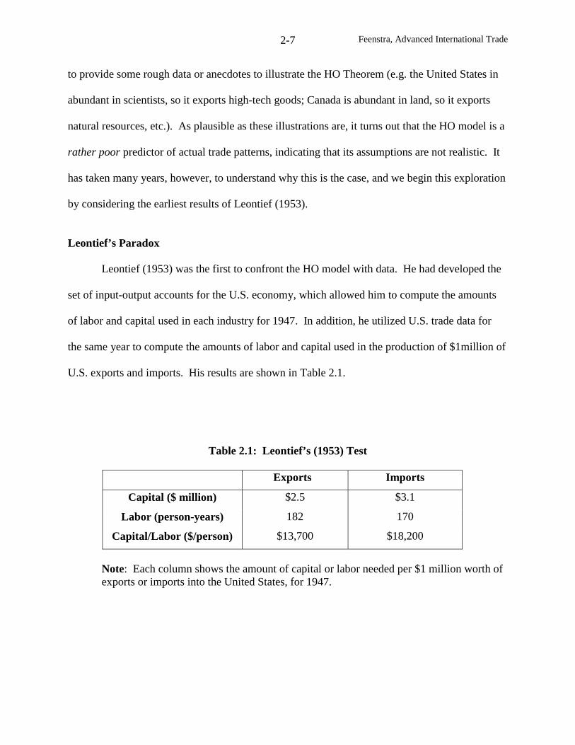
U.S. exports and imports. His results are shown in Table 2.1.
Table 2.1: Leontief’s (1953) Test
Exports Imports
Capital ($ million) $2.5 $3.1
Labor (person-years) 182 170
Capital/Labor ($/person) $13,700 $18,200
Note: Each column shows the amount of capital or labor needed per $1 million worth ofexports or imports into the United States, for 1947.
Feenstra, Advanced International Trade2-8
Leontief first measured the amount of capital and labor required for $1 million worth of
U.S. exports. This calculation requires that we measure the labor and capital used directly, i.e. in
each exporting industry, and also these factors used indirectly, i.e. in the industries that produce
intermediate inputs that are used in producing exports. From the first row of Table 2.1, we see
that $2.5 million worth of capital was used in $1 million of exports. This amount of capital
seems much too high, until we recognize that what is being measured is the capital stock, so that
only the annual depreciation on this stock is actually used. For labor, 182 person-years was used
to produce the exports. Taking the ratio of these, we find that each person employed in
producing exports (directly or indirectly) is working with $13,700 worth of capital.
Turning to the import side of the calculation, we immediately run into a problem: it is
not possible to measure the amount of labor and capital used in producing imports unless we
have knowledge of the foreign technologies, which Leontief certainly did not know in 1953!
Indeed, it is only very recently that researchers have begun to use data on foreign technologies to
test the HO model, as we will describe later in the chapter. So Leontief did what many
researchers have done since: he simply used the U.S. technology to calculate the amount of labor
and capital used in imports. Does this invalidate the test of the HO model? Not really, because
recall that an assumption of the HO model is that technologies are the same across countries.
Thus, under the null hypothesis that the HO model is true, it would be valid to use the U.S.
technology to measure the labor and capital used in imports. If we find that this null hypothesis
is rejected, then one explanation would be that the assumption of identical technologies is false.
Using the U.S. technology to measure the labor and capital used in imports, both directly
and indirectly, we arrive at the estimates in the last column of Table 2.1: $3.1 million of capital,
170 person-years, and so a capital/labor ratio in imports of $18,200. Remarkably, this is higher
Feenstra, Advanced International Trade2-9
than the capital/labor ratio found for U.S. exports! Under the presumption that the U.S. was
capital-abundant in 1956, this appears to contradict the HO Theorem. Thus, this finding came to
be called “Leontief’s Paradox.”
A wide range of explanations have been offered for this paradox:
• U.S. and foreign technologies are not the same;
• By focusing only on labor and capital, Leontief ignored land;
• Labor should have been disaggregated by skill (since it would not be surprising to find that
U.S. exports are intensive in skilled labor);
• The data for 1947 may by unusual, since World War II had just ended;
• The U.S. was not engaged in free trade, as the HO model assumes.
These reasons are all quite valid criticisms of the test that Leontief performed, and
research in the years following his test aimed to re-do the analysis while taking into account
land, skilled versus unskilled labor, checking other years, etc. This research is well summarized
by Deardorff (1984a), and the general conclusion is that the paradox continued to occur in some
cases. It was not until two decades later, however, that Leamer (1980) provided the definitive
critique of the Leontief paradox: it turned out that Leontief had performed the wrong test! That
is, even if the HO model is true, it turns out the capital/labor ratios in export and imports, as
reported in Table 2.1, should not be compared. Instead, an alternative test should be performed.
The test that Leamer proposed relies on the “factor content” version of the Heckscher-Ohlin
model, developed by Vanek (1968), which we turn to next.
Feenstra, Advanced International Trade2-10
Heckscher-Ohlin-Vanek (HOV) Model
Let us now consider many countries, indexed by i = 1,…,C; many industries, indexed by
j=1,…,N; and many factors, indexed by k, l =1,..,M. We will continue to assume that
technologies are identical across countries, and that factor-price equalization prevails under free
trade. In addition, we assume that tastes are identical and homothetic across countries.
Let the (MxN) matrix A=[ajk]' denote the amounts of labor, capital, land, and other
primary factors needed for one unit of production in each industry.4 Notice that this matrix
applies in any country. The rows measure the different factors k, l =1,…,M, while the columns
of this matrix measure the different industries j=1,…,N. For example, with just two industries
using only labor and capital, this matrix would be A =
K2K1
L2L1
aa
aa.
Next, let Yidenote the (Nx1) vector of outputs in each industry for country i, and let D
i
denote the (Nx1) vector of demands of each good, so that Ti=Y
i– D
iequals the vector of net
exports for country i. The factor content of trade is then defined as Fi ≡ AT
i, which is an (Mx1)
vector. We will denote individual components of this vector as ikF , where a positive value
indicates that the factor is exported, while a negative value indicates that the factor is imported.
For example, with just labor and capital, the factor content of trade is ≡
ik
i
F
Fl ATi.
The goal of the HOV model is to relate the factor content of trade ATito the underlying
4 This matrix should include both the direct primary factors used in the production of each good, as well as theindirect primary factors used through the intermediate inputs. In practice, the indirect factors are measured using theinput-output matrix for the economy. That is, denoting the (MxN) direct factor requirements by A
~ and the (MxM)
input-output matrix by B, we compute the total factor requirements as 1)BI(A
~A
−−= .
Feenstra, Advanced International Trade2-11
endowments of country i. To do so, we can proceed by computing AYiand AD
i. The term AYi
equals the demand for factors in country i. Analogous to the full-employment conditions studied
in chapter 1, AYiequals the endowments of country i, which we write as AY
i= V
i. Turning to
ADi, this terms is simplified by using our assumption of identical and homothetic tastes. Since
product prices are equalized across countries by free trade, it follows that the consumption
vectors of all countries must be proportional to each other. We shall write this as Di= s
iD
w,
where Dw
denotes the world consumption vector and siis the share of country i in world
consumption. It follows that ADi= s
iAD
w. Note that if trade is balanced, then s
ialso equals
country i’s share of world GDP.5 Since world consumption must equal world production, we
therefore obtain ADi= s
iAD
w= s
iAY
w= s
iV
w, where the last equality is the full-employment
condition at the world level.
Making use of these expressions for AYiand AD
i, we have therefore proved:
Fi ≡ AT
i= V
i– s
iV
w, (2.1)
which is a statement of the Heckscher-Ohlin-Vanek (HOV) Theorem. In terms of individual
factors, this is written as wk
iik
ik VsVF −= . If country i’s endowment of factor k relative the
world endowment exceeds country i’s share of world GDP ( iwk
ik s/VV > ), then we say that
country i is abundant in that factor. In that case, (2.1) says that the factor-content of trade in
factor k should also be positive ( 0Fik > ), and conversely if country i is scarce in factor k
5 Letting p denote the vector of prices, in general, p′Di=s
ip′D
w, so that s
i= p′D
i/ p′D
w. If trade is balanced
then we also have wiwiiGDP/GDPY'p/Y'ps == .
Feenstra, Advanced International Trade2-12
( iwk
ik s/VV < ).
What does the HOV Theorem tell us about the Leontief test? To anwer this, let us focus
on just two elements of the factor-content vector, for labor and capital. These are written as:
ikF = K
i– s
iK
w, (2.2a)
iFl = Li– s
iL
w, (2.2b)
where ikF and iFl are the computed factor contents of trade, and Ki and Li are the capital and
labor endowments for country i. Following Leamer (1980), we define capital to be abundant
relative to labor in country i if Ki/K
w> L
i/L
w. Then using (2.2), the implications of capital
abundance are:
Theorem (Leamer, 1980)
If capital is abundant relative to labor in country i, then the HOV Theorem (2.1) implies that the
capital/labor ratio embodied in production for country i exceeds the capital/labor ratio embodied
in consumption:
Ki/L
i> (K
i– i
kF )/( Li– iFl ) . (2.3)
Proof:
From equation (2.2), we have Kw = (Ki – ikF )/ si and Lw = (Li – iFl )/ si . It follows that
Ki/Kw = si Ki /(Ki – ikF ) and L i /Lw = si Li /(Li – iFl ). Then Ki /Kw > Li /Lw implies that
Ki /(Ki – ikF ) > Li /(Li – iFl ), which is rewritten as (2.3) . QED
Feenstra, Advanced International Trade2-13
To interpet this result, note that Kiand L
iare simply the endowments of capital and labor,
or alternatively, the capital and labor embodied in production. If we subtract the content of these
factors embodied in trade, then what we end up with can be defined as the factor-content of
consumption, or Ki– i
kF and Li– iFl . Then equation (2.3) states that the capital/labor ratio
embodied in production (on the left) must exceed the capital/labor ratio embodied in
consumption (on the right).
The results from making this comparison for the U.S. in 1947 are shown in Table 2.2. In
the first column we list the capital and labor endowments for the U.S., and in the second column
we show the capital and labor embodied in consumption. Taking the ratio of these, it is indeed
the case that the capital/labor ratio embodied in production exceeds that in consumption. This is
the precise application of the HOV Theorem, and it turns out to be satisfied for the U.S. in 1947,
contrary to what Leontief concluded. Thus, there was no paradox after all!
It is useful to see the HOV Theorem and Leamer’s result in a diagram. In Figure 2.3, the
length of the horizontal axis is the world labor endowment Lw
= L1+L
2, and the length of the
vertical axis is the world capital endowment Kw
= K1+K
2. The origin for country 1 is in the
lower-left corner, and for country 2 is in the upper-right corner. Thus, any point in the world
endowment box measures the endowments (Li, K
i) of the two countries. Suppose that the
endowments are at the point Vi, where country 1 is labor-abundant, L1/K
1> L
w/K
w> L
2/K
2.
Under the assumptions of the HOV model, the consumption of each country Diis
proportional to world consumption Dw
, which means that the factor content of consumption ADi
is proportional to ADw
= Vw
. In other words, the factor-content of consumption must lie along
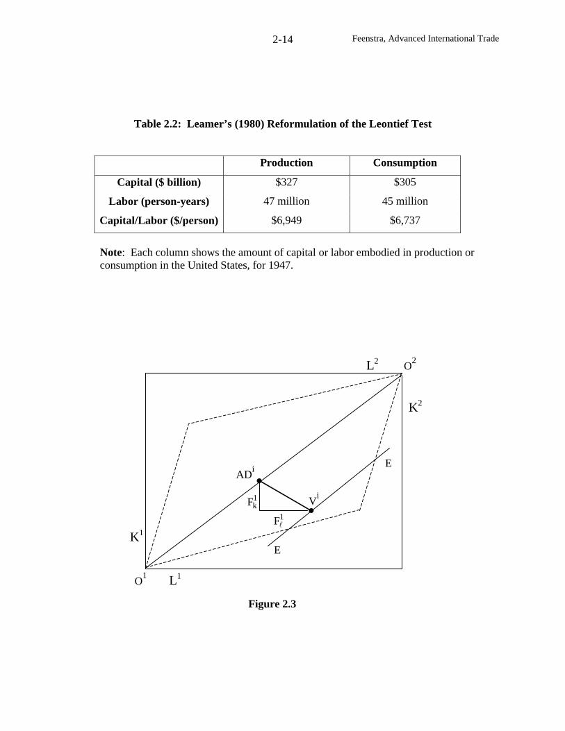
Feenstra, Advanced International Trade2-14
Table 2.2: Leamer’s (1980) Reformulation of the Leontief Test
Production Consumption
Capital ($ billion) $327 $305
Labor (person-years) 47 million 45 million
Capital/Labor ($/person) $6,949 $6,737
Note: Each column shows the amount of capital or labor embodied in production orconsumption in the United States, for 1947.
E
1kF
1Fl
EAD
i
Vi
O1 L1
K1
K2
L2 O2
Figure 2.3
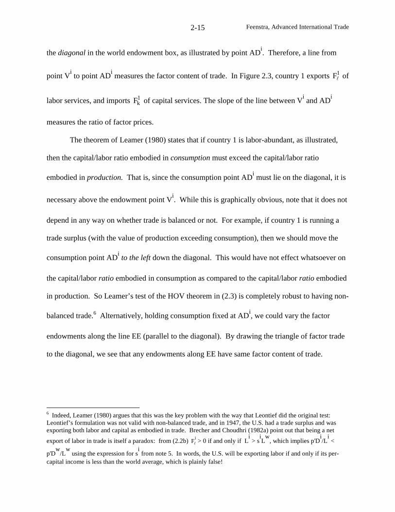
Feenstra, Advanced International Trade2-15
the diagonal in the world endowment box, as illustrated by point ADi. Therefore, a line from
point Vito point AD
imeasures the factor content of trade. In Figure 2.3, country 1 exports 1Fl of
labor services, and imports 1kF of capital services. The slope of the line between V
iand AD
i
measures the ratio of factor prices.
The theorem of Leamer (1980) states that if country 1 is labor-abundant, as illustrated,
then the capital/labor ratio embodied in consumption must exceed the capital/labor ratio
embodied in production. That is, since the consumption point ADimust lie on the diagonal, it is
necessary above the endowment point Vi. While this is graphically obvious, note that it does not
depend in any way on whether trade is balanced or not. For example, if country 1 is running a
trade surplus (with the value of production exceeding consumption), then we should move the
consumption point ADito the left down the diagonal. This would have not effect whatsoever on
the capital/labor ratio embodied in consumption as compared to the capital/labor ratio embodied
in production. So Leamer’s test of the HOV theorem in (2.3) is completely robust to having non-
balanced trade.6 Alternatively, holding consumption fixed at ADi, we could vary the factor
endowments along the line EE (parallel to the diagonal). By drawing the triangle of factor trade
to the diagonal, we see that any endowments along EE have same factor content of trade.
6 Indeed, Leamer (1980) argues that this was the key problem with the way that Leontief did the original test:Leontief’s formulation was not valid with non-balanced trade, and in 1947, the U.S. had a trade surplus and wasexporting both labor and capital as embodied in trade. Brecher and Choudhri (1982a) point out that being a net
export of labor in trade is itself a paradox: from (2.2b) iFl > 0 if and only if L
i> s
iL
w, which implies p'D
i/L
i<
p'Dw
/Lw
using the expression for si
from note 5. In words, the U.S. will be exporting labor if and only if its per-capital income is less than the world average, which is plainly false!
Feenstra, Advanced International Trade2-16
Partial Tests of the HOV Theorem
The statement of the HOV Theorem in (2.1) tells us immediately how a complete test of
the theory should by performed: simply compute the left-hand side (using data on trade Tiand
technology A), compute the right-hand side (using data on endowments Viand V
w), and
compare them. Depending on how well they match up, we can judge whether the Theorem is an
empirical success or not. This complete test requires both trade and endowments data for many
countries, and technology data for at least one country. While such data is readily available
today,7 this was not the case two or three decades ago. Accordingly, many researchers, including
Leontief himself, performed what we can call “partial tests” of the HOV model, using only two
rather than all three types of data. Before considering the complete test, we will review several
other partial tests that were performed.
Let us assume that the number of goods equals the number of factors, so that A is a
square matrix, which we assume is invertible. Then we can re-write (2.1) as:
Ti
= A-1
(Vi
– siV
w) . (2.4)
This equation could be tested in several ways. First, if we think about the matrix A-1
as data,
then we could run a regression of Tion A
-1, and coefficients obtained would serve as an estimate
of the relative abundance (Vi
– siV
w) of each factor. Baldwin (1971) performed a test similar to
this, but instead of regressing Tion A
-1, he actually regressed T
ion 'A . With two factors and
7 Input-output tables as well as bilateral trade data for many countries over 1976-1999 is available from the WorldBank at: www1.worldbank.org/wbiep/trade/tradeandproduction.html. Also see the trade and production dataavailable at: www.internationaldata.org.
Feenstra, Advanced International Trade2-17
three goods, for example, 'A is the matrix
K3L3
K2L2
K1L1
aa
aa
aa
. Thus, Baldwin regressed the adjusted
net exports of each industry8 on their labor and capital requirements needed for one unit of
production.
Using data for 60 U.S. industries for years around 1960, and disaggregating workers by
their types, Baldwin (1971) obtained the following result:
Adjusted net exports = –1.37*
(Physical Capital/Worker) + 7011*
(Scientists/Worker)
– 1473 (Managers/Worker) + 71 (Clerical Staff/Worker)
+ 1578*
(Craftsmen & Foremen/Worker) + 248 (Operatives/Worker)
+ 761 (Unskilled Employee/Worker) + 845*
(Farmers/Worker)
+ (Other variables included for industry scale and unionization),
N=60, R2=0.44, * = significant at 95% level
Thus, looking across the U.S. industries, Baldwin finds that those industries using more
scientist, craftsmen and foremen, or farmers relative to total workers, will tend to have higher
exports. The importance of scientists and farmers in predicting U.S. exports is not surprising at
all, since the U.S. is abundant in skilled–labor and land; and the importance of craftsmen and
foremen is perhaps reasonable, too. What is surprising, however, is the negative coefficient
found on the very first variable, physical capital/worker. Taken literally, this coefficient says
that U.S. industries using more capital/worker will tend to export less. This is exactly the
8 Adjusted net exports are defined as industry exports per million dollars of total exports minus industry importsper million dollars of total imports.
Feenstra, Advanced International Trade2-18
opposite of what we would expect if the U.S. were capital-abundant. Thus, this result appears to
be similar to the “paradox” found by Leontief.
Various writers after Baldwin have redone the type of regression shown above, with
mixed results: sometimes the capital coefficient is positive, but other times it is again negative
(see the survey by Deardorff, 1984a). What are we to make of these results? Well, as we argued
for Leontief’s original paradox, it can be questioned whether Baldwin’s approach is a valid test
of the HOV model. From (2.4), a valid test would be to regress Tion A
-1, but instead, Baldwin
regressed Tion 'A . To see the consequences of this, use the ordinary least squares (OLS)
formula for the coefficients β that would be obtained from this regression:
)VsV()AA(AT)AA(ˆAT wii1i1i −′=′=β⇒β′= −− , (2.5)
where the final equality follows from using the HOV Theorem (2.1).
Thus, we see that β is a contaminated estimate of the vector of relative factor
endowments (Vi
– siV
w). Namely, rather than equaling the relative factor endowments vector,
β equals the positive definite matrix (AA')-1
times (Vi
– siV
w). Because (AA')
-1is certainly not
the identity matrix, it is entirely possible that the sign pattern of the elements in β will differ
from the sign pattern of (Vi
– siV
w).9 In other words, even if the U.S. was capital-abundant and
the HOV Theorem held, it would still be possible for the Baldwin regression to find a negative
coefficient on capital: this does not contradict the HOV Theorem, because like the original
Leontief approach, it is the wrong test.
9 See Leamer and Bowen (1981) and Aw (1983).
Feenstra, Advanced International Trade2-19
The careful reader might point out, however, that possible differences in the sign pattern
of β and (Vi
– siV
w) can presumably be checked for using the actual data on (AA')
-1. This is
exactly the approach taken by Bowen and Sveikaukus (1992), who argue that such sign reversals
are very unlikely to occur in practice. Thus, the Baldwin regression may be acceptable in
practice, and in fact, it has been used in recent research by Romalis (2001).10 As a descriptive
tool to show how trade is related to industry factor requirements this regression makes good
sense, but as a definitive test of the HOV Theorem it is inadequate for the reasons we have
described.
A second “partial test” of the HOV Theorem in equation (2.4) has been used by Leamer
(1984). In contrast to Baldwin, Leamer tested (2.4) by treating factor endowments (Vi
– siV
w)
as data, while estimating the elements of A-1
. To describe this test, notice that (2.4) applies
across all countries i. Focusing on a single industry j, and letting the elements of A-1
be written
as jkβ , we can write (2.4) in scalar form as:
∑=
−β=N
1k
wk
iikjk
ij )VsV(T , i = 1,…,C. (2.6)
Notice that the summation in (2.6) is across factors, while the observations are across countries.
Thus, to estimate this regression we would combine the observation for a single industry j across
multiple countries i=1,…,C, where the coefficients βjk are estimated. These coefficients
should be interpreted as Rybczynski effects, and as shown in chapter 1, can be positive or
negative.
10 Romalis’ model relies on the monopolistic competition framework, which we do not cover until chapter 5. It isrecommended for further reading after that.
Feenstra, Advanced International Trade2-20
To run this regression, we first need to choose some aggregation scheme for net exports
and factors of production. Leamer (1984) works with the trade data for 60 countries in two
years, 1958 and 1975. The trade data is organized according to the Standard Industrial Trade
Classification (SITC). Because these are traded goods, they include only merchandise, i.e.
agriculture, mining and manufacturing. Leamer organizes these goods into 10 aggregates, as
shown in the first column of Table 2.3: two primary products (petroleum and raw materials);
four crops (forest products, tropical agricultural products, animal products and cereals); and four
manufactured products (labor-intensive manufactures, capital-intensive manufactures, machinery
and chemicals).11 Implicitly there is an eleventh product in the economy, making up all the non-
traded goods, so Leamer includes total GNP as an aggregate to reflect this. There are also eleven
factors of production, listed along the top row of Table 2.3: capital, three types of workers
(distinguished by skill), four types of land (distinguished by climate), and three natural resources.
So the number of goods equals the number of factors by construction.
The estimates of jkβ from regressing the 1975 net exports of each of these aggregates on
the country factor endowments are shown in Table 2.3. Leamer stresses that the point estimates
should not be taken too seriously, but the sign pattern of the coefficients is of interest, especially
when the estimates are significantly different from zero. In interpreting the coefficients as
Rybczynski effects, it is noteworthy to recall that an increase in the capital endowment is
11 The method used to form these aggregates involves looking at the cross-country correlations of the disaggregateproducts in each group with the aggregate itself. That is, “cereals” is an aggregate because countries that export thisin total tend to have high exports of all the products within this group. It turns out that the ratios of capital/workerand professional/all workers are also reasonably similar within the aggregates. Feenstra and Hanson (2000) considerhow the aggregation scheme might lead to bias in calculations of the factor content of trade.
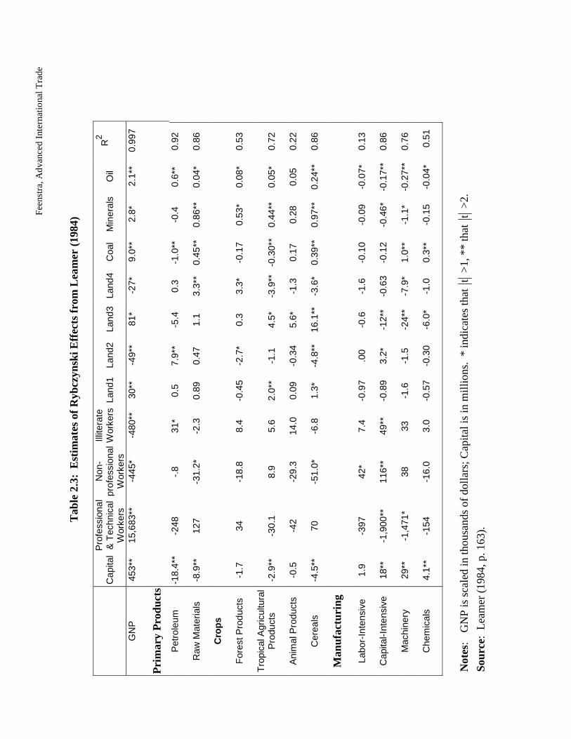
Fee
nstr
a,A
dvan
ced
Inte
rnat
iona
lTra
de
Tab
le2.
3:E
stim
ates
ofR
ybcz
ynsk
iEff
ects
from
Lea
mer
(198
4)
Cap
ital
Pro
fess
iona
l&
Tec
hnic
alW
orke
rs
Non
-pr
ofes
sion
alW
orke
rs
Illite
rate
Wor
kers
Land
1La
nd2
Land
3La
nd4
Coa
lM
iner
als
Oil
R2
GN
P45
3**
15,6
83**
-445
*-4
80**
30**
-49*
*81
*-2
7*9.
0**
2.8*
2.1*
*0.
997
Pri
mar
yP
rodu
cts
Pet
role
um-1
8.4*
*-2
48-.
831
*0.
57.
9**
-5.4
0.3
-1.0
**-0
.40.
6**
0.92
Raw
Mat
eria
ls-8
.9**
127
-31.
2*-2
.30.
890.
471.
13.
3**
0.45
**0.
86**
0.04
*0.
86
Cro
ps
For
estP
rodu
cts
-1.7
34-1
8.8
8.4
-0.4
5-2
.7*
0.3
3.3*
-0.1
70.
53*
0.08
*0.
53
Tro
pica
lAgr
icul
tura
lP
rodu
cts
-2.9
**-3
0.1
8.9
5.6
2.0*
*-1
.14.
5*-3
.9**
-0.3
0**
0.44
**0.
05*
0.72
Ani
mal
Pro
duct
s-0
.5-4
2-2
9.3
14.0
0.09
-0.3
45.
6*-1
.30.
170.
280.
050.
22
Cer
eals
-4.5
**70
-51.
0*-6
.81.
3*-4
.8**
16.1
**-3
.6*
0.39
**0.
97**
0.24
**0.
86
Man
ufac
turi
ng
Labo
r-In
tens
ive
1.9
-397
42*
7.4
-0.9
7.0
0-0
.6-1
.6-0
.10
-0.0
9-0
.07*
0.13
Cap
ital-I
nten
sive
18**
-1,9
00**
116*
*49
**-0
.89
3.2*
-12*
*-0
.63
-0.1
2-0
.46*
-0.1
7**
0.86
Mac
hine
ry29
**-1
,471
*38
33-1
.6-1
.5-2
4**
-7.9
*1.
0**
-1.1
*-0
.27*
*0.
76
Che
mic
als
4.1*
*-1
54-1
6.0
3.0
-0.5
7-0
.30
-6.0
*-1
.00.
3**
-0.1
5-0
.04*
0.51
Not
es:
GN
Pis
scal
edin
thou
sand
sof
dolla
rs;C
apita
lis
inm
illio
ns.
*in
dica
tes
that
t>
1,**
that
t>
2.
Sour
ce:
Lea
mer
(198
4,p.
163)
.
Feenstra, Advanced International Trade
associated with a rise in the net exports of all the manufactured goods, and the same is true for an
increase in the endowments of nonprofessional or illiterate workers. Conversely, increases in
most types of land, or of professional and technical workers, are associated with declines in the
net exports of the manufactured products. The interpretation of these results is that increases in
land favor agriculture over manufacturing, and increases in professional and technical workers
favor non-traded services over manufacturing.
Because the estimated coefficients can be positive or negative they do not provide any
basis to test the HOV Theorem. Instead, we have to rely on the overall fit of the regression: a
linear relationship between endowments and trade, as in (2.6), is implied by the theory and can
be assessed by the R2
of the regressions. In the final column of Table 2.3 we show the R2 from
each cross-country regression, and these vary from 0.13 to nearly unity. Admittedly, these fits
are a very weak test of the theory, because we generally do not want to rely on only the R2
of an
equation to judge the validity of the theory underlying it. So while this early approach of Leamer
(1984) provides interesting results on the Rybczynski effects (as we shall refer to again in the
next chapter), it is of limited usefulness in testing the HOV Theorem.
We summarize our results so far in Table 2.4, which indicates the data used and the basic
methods of the various authors. These various “partial tests” have used only two sources of data,
and we now turn to various complete tests of the HOV Theorem, using all three sources of data
(trade, technology and factor endowments).
Complete Test of the HOV Theorem
The first complete test of the HOV theorem was by Bowen, Leamer and Sveikaukas
(1987). They proposed two tests of equation (2.1):
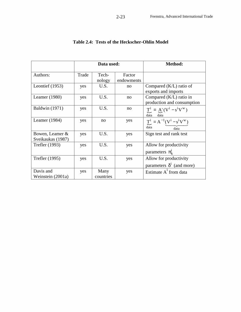
Feenstra, Advanced International Trade2-23
Table 2.4: Tests of the Heckscher-Ohlin Model
Data used: Method:
Authors: Trade Tech-nology
Factorendowments
Leontief (1953) yes U.S. no Compared (K/L) ratio ofexports and imports
Leamer (1980) yes U.S. no Compared (K/L) ratio inproduction and consumption
Baldwin (1971) yes U.S. no{ { )VsV('AT wii
datadata
i −=
Leamer (1984) yes no yes{ 43421
data
wii1
data
i )VsV(AT −= −
Bowen, Leamer &Sveikaukas (1987)
yes U.S. yes Sign test and rank test
Trefler (1993) yes U.S. yes Allow for productivity
parameters ikπ
Trefler (1995) yes U.S. yes Allow for productivity
parameters iδ (and more)Davis andWeinstein (2001a)
yes Manycountries
yes Estimate Aifrom data
Feenstra, Advanced International Trade2-24
Sign test: sign( ikF ) = sign( i
kV – si w
kV ), i=1,…,C; k=1,…,M;
Rank test: ikF > iFl ⇔ ( i
kV – si w
kV ) > ( iVl – si wVl ), i=1,…,C; k=1,…,M.
The first of these tests simply compares the sign pattern on the left and right of (2.1). With M
factors and C countries, there are MC observations in total, and we are interested in what
percentage of these have the same sign on the two sides of the equation. Notice that a
completely random pattern of signs such as obtained by flipping a coin would still generate
correct signs 50% of the time in a large sample. Therefore, the sign test must do considerably
better than this in order to conclude that the HOV Theorem is successful.
The rank test involves a pairwise comparison of all factors for each country, so there are
M(M–1)/2 pairs for each of C countries. If the computed factor contents of one factor exceeds
that of a second factor, then we check whether the relative abundance of that first factor also
exceeds the relative abundance of the second factor. Again, a completely random assignment of
factor abundance and relative endowments would imply that in 50% of the comparisons in a
large sample, the rank test would be satisfied, so we would hope that the actual data perform
considerably better than this.
In fact, the sign and rank test both fail miserably when confronted with actual data.
Using data for 27 countries and 12 factors, Bowen, Leamer and Sveikaukas found that the sign
test was satisfied in about 61% of the cases, and the rank test was satisfied in about 49% of the
cases: about what we would expect from flipping a coin. These negative results were confirmed
in later calculations by Trefler (1995), with a sample of 33 countries and 9 factors, and his results
for each country are shown in Table 2.5. Overall, the sign test was successful in only 50% of the
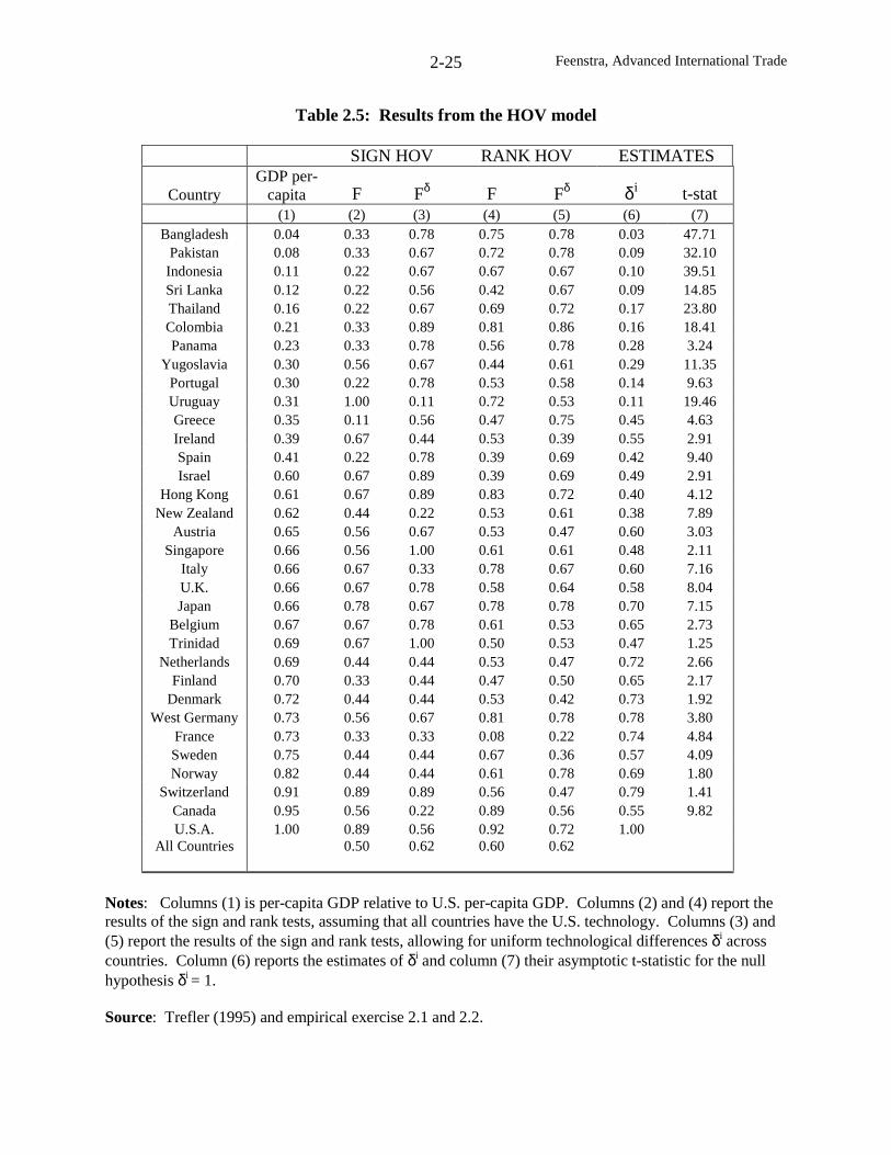
Feenstra, Advanced International Trade2-25
Table 2.5: Results from the HOV model
SIGN HOV RANK HOV ESTIMATES
CountryGDP per-
capita F Fδ F Fδ iδ t-stat(1) (2) (3) (4) (5) (6) (7)
Bangladesh 0.04 0.33 0.78 0.75 0.78 0.03 47.71Pakistan 0.08 0.33 0.67 0.72 0.78 0.09 32.10
Indonesia 0.11 0.22 0.67 0.67 0.67 0.10 39.51Sri Lanka 0.12 0.22 0.56 0.42 0.67 0.09 14.85Thailand 0.16 0.22 0.67 0.69 0.72 0.17 23.80Colombia 0.21 0.33 0.89 0.81 0.86 0.16 18.41Panama 0.23 0.33 0.78 0.56 0.78 0.28 3.24
Yugoslavia 0.30 0.56 0.67 0.44 0.61 0.29 11.35Portugal 0.30 0.22 0.78 0.53 0.58 0.14 9.63Uruguay 0.31 1.00 0.11 0.72 0.53 0.11 19.46Greece 0.35 0.11 0.56 0.47 0.75 0.45 4.63Ireland 0.39 0.67 0.44 0.53 0.39 0.55 2.91Spain 0.41 0.22 0.78 0.39 0.69 0.42 9.40Israel 0.60 0.67 0.89 0.39 0.69 0.49 2.91
Hong Kong 0.61 0.67 0.89 0.83 0.72 0.40 4.12New Zealand 0.62 0.44 0.22 0.53 0.61 0.38 7.89
Austria 0.65 0.56 0.67 0.53 0.47 0.60 3.03Singapore 0.66 0.56 1.00 0.61 0.61 0.48 2.11
Italy 0.66 0.67 0.33 0.78 0.67 0.60 7.16U.K. 0.66 0.67 0.78 0.58 0.64 0.58 8.04Japan 0.66 0.78 0.67 0.78 0.78 0.70 7.15
Belgium 0.67 0.67 0.78 0.61 0.53 0.65 2.73Trinidad 0.69 0.67 1.00 0.50 0.53 0.47 1.25
Netherlands 0.69 0.44 0.44 0.53 0.47 0.72 2.66Finland 0.70 0.33 0.44 0.47 0.50 0.65 2.17
Denmark 0.72 0.44 0.44 0.53 0.42 0.73 1.92West Germany 0.73 0.56 0.67 0.81 0.78 0.78 3.80
France 0.73 0.33 0.33 0.08 0.22 0.74 4.84Sweden 0.75 0.44 0.44 0.67 0.36 0.57 4.09Norway 0.82 0.44 0.44 0.61 0.78 0.69 1.80
Switzerland 0.91 0.89 0.89 0.56 0.47 0.79 1.41Canada 0.95 0.56 0.22 0.89 0.56 0.55 9.82U.S.A. 1.00 0.89 0.56 0.92 0.72 1.00
All Countries 0.50 0.62 0.60 0.62
Notes: Columns (1) is per-capita GDP relative to U.S. per-capita GDP. Columns (2) and (4) report theresults of the sign and rank tests, assuming that all countries have the U.S. technology. Columns (3) and(5) report the results of the sign and rank tests, allowing for uniform technological differences δi acrosscountries. Column (6) reports the estimates of δi and column (7) their asymptotic t-statistic for the nullhypothesis δi = 1.
Source: Trefler (1995) and empirical exercise 2.1 and 2.2.
Feenstra, Advanced International Trade2-26
cases when using the U.S. technology to measure the matrix A (column (2) in Table 2.5).12 The
rank test was successful in only 60% of cases (column 4). This lack of success indicates that
some assumption of the HOV model is drastically wrong!
Trefler (1995) performs several diagnostic tests on the data to determine which
assumptions of the HOV model is most likely to be responsible for its failure, and concludes that
the assumption of equal technologies across countries is especially bad. Accordingly, he
develops an extended version of the HOV model that allows for different technologies across
countries, as originally proposed by Leontief (1953) as one explanation for the “paradox.”
Modeling Different Technologies Across Countries
There are two ways that technological differences can be introduced into the HOV model.
One approach is to model the productivity of factors in different countries, whereas another
approach is to model differences in the factor requirements matrix A. These approaches are
closely related, of course: saying that a factor is 10% less productive in one country is the same
as saying that 10% more of that factor is needed per unit of production. But thinking about them
as distinct will be convenient for our discussion.
Trefler (1993) takes the first approach, and allows all factors in every country to differ in
their productivities. The only exception to this is for the U.S., which he uses as the benchmark
country, with factor productivities normalized at unity. So let ikπ denote the productivity of
factor k in country i relative to its productivity in the U.S. In terms of efficiency units, the
12 Table 2.5 corrects the expenditure shares si
for trade imbalance. From note 6, si
= p′Di
/ p′Dw
. Noting that
GDPi
= p′Yi
= p′Di
+ p′Ti, it follows that when p′T
i≠ 0 due to trade imbalances, we should measure the shares by
si
= (GDPi
– p′Ti
)/ GDPw
.
Feenstra, Advanced International Trade2-27
effective endowment of factor k in country i becomes ik
ikVπ . Let A now denote the amount of
effective factors needed per unit of output in each industry. We continue to assume that factor-
price equalization holds in terms of effective factor prices, so with identical technologies, the
matrix A is the same across countries. Thus, we continue to measure the factor-content of trade
as Fi ≡ AT
i. Then the HOV equation (2.1) is re-written in terms of effective factor endowments
as:
ikF = i
kikVπ – s
i jk
jk
C
1jVπ∑
=, i=1,…,C; k=1,…,M. (2.7)
There are MC equations in (2.7), and M(C–1) productivity parameters. These equations
are not independent, however. For any factor k, if we sum (2.7) across countries i=1,…,C then
we must obtain zero on both sides: exports equal imports for the world, even when measured in
terms of factor contents. So we can drop the equations for one country, and we do so for the
U.S. This leaves M(C–1) equations in M(C–1) parameters. These equations will be independent
“almost everywhere,” i.e. for almost all sets of data on endowments and factor-contents of trade.
Furthermore, the productivity parameters enter (2.7) linearly, so the M(C–1) equations in (2.7)
can be inverted to solve for these uniquely. Thus, we have established:
Theorem (Trefler, 1993)
Allowing for all factors in all but one country to differ in their productivities ikπ , for almost all
datasets there will be a solution for productivities ikπ such that the HOV equation (2.7) hold with
equality for i=1,…,C, k=1,…,M.
The unusual feature of this result is that the HOV equation no longer becomes testable: it
holds as an identity by the choice of productivity parameters! How, then, are we to judge
Feenstra, Advanced International Trade2-28
whether the HOV model is a reasonable description of reality or not? Trefler recommends two
methods: first, we need to check whether the productivity parameters are positive (there is
nothing in the inversion of (2.7) that guarantees this); second, we might compare these
parameters to other economic data to evaluate how “reasonable” the productivity parameters are.
For example, it makes sense to compare the labor productivity parameters to wages across
countries. If factor-price equalization holds in terms of effective endowments, then it should be
the case that the productivity parameters ikπ match the factor prices of country i quite closely.
In Figure 2.4, we show the results that Trefler (1993) obtains for labor.13 On the
horizontal axis we measure the estimated productivities ilπ , and on the vertical axis is data on
wages across countries (both of these are relative to the U.S.). It is clear that the observations on
these two variables across countries follow each other quite closely: the correlation between
estimated ilπ and actual wages is 0.9. Since we think that cross-country differences in wages
should indeed reflect workers productivities, this close correspondence between the two in
Figure 2.4 lends support to Trefler’s extension of the HOV model.14
Turning to the second method of introducing productivity differences, Trefler (1995)
allows the factor requirements matrix Aito differ across countries, while assuming that the factor
endowments do not differ in efficiency units. In this paper, he chooses to restrict the range of
differences in matrices Aiso that the HOV equations give less than a perfect fit. This means that
13 In empirical exercise 2.3 you are provided with Trefler’s data and are asked to compute the productivities ikπ .
14 Gabaix (1999) disagrees, and argues that even when the labor content of trade is zero the solution for the
productivities of labor ilπ from equation (2.7) is simply GDP per-capita, as you are asked to show in problem 2.1.
Because the labor content of trade is small, it is therefore not surprising that the solution for ilπ is highly correlated
with wages, which are highly correlated with GDP per-capita.
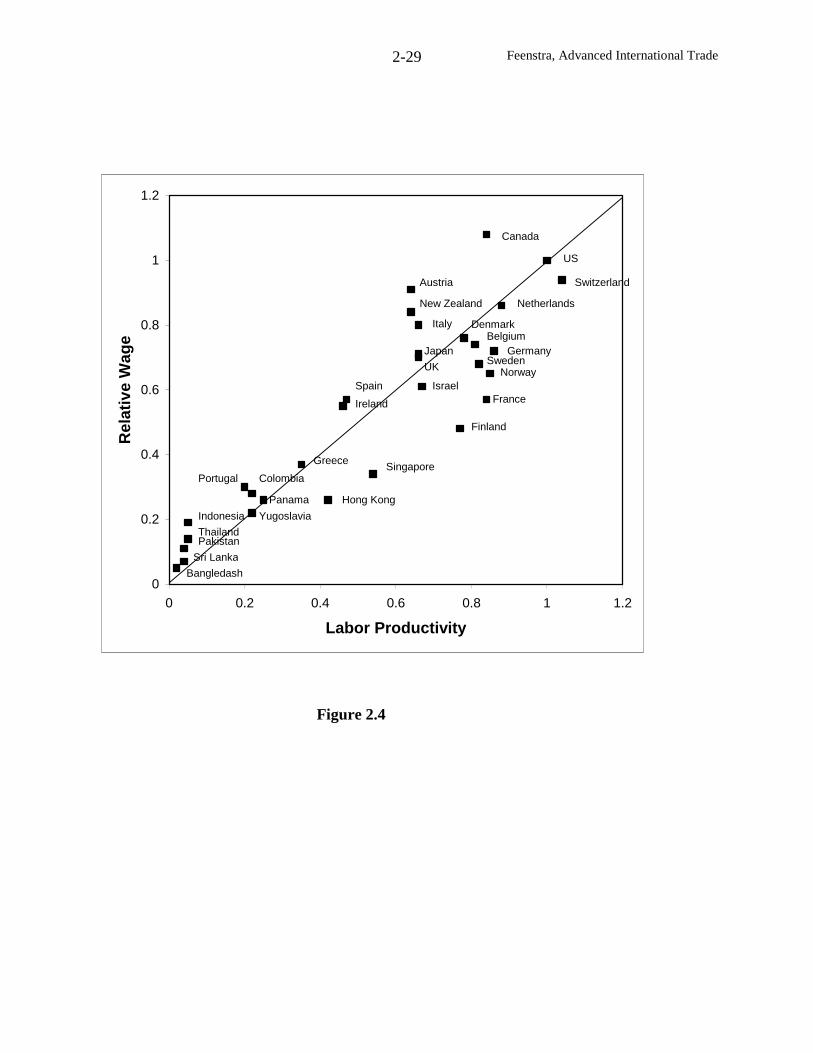
Feenstra, Advanced International Trade2-29
0
0.2
0.4
0.6
0.8
1
1.2
0 0.2 0.4 0.6 0.8 1 1.2
Labor Productivity
Rel
ativ
eW
age
Canada
Switzerland
US
Netherlands
Austria
New Zealand
Italy DenmarkBelgium
GermanySweden
Norway
France
Japan
UK
Israel
Finland
Spain
Ireland
Singapore
Hong Kong
Greece
Bangledash
Sri Lanka
PakistanThailand
Indonesia Yugoslavia
Panama
Portugal Colombia
Figure 2.4
Feenstra, Advanced International Trade2-30
we are back in the traditional econometric approach: choosing the parameters of Aiso as to
minimize the sum of squared residuals of the HOV equations. To implement this, we need to
model Aiin terms of some productivity differences across countries. The initial case that Trefler
considers is where the matrices Aidiffer by a uniform amount across countries:
USii AA =δ , (2.8)
which implies iUSi /AA δ= . With δi< 1, this means that A
i> A
US, so that country i is less
productive and requires more labor, capital, and other resources for a unit of production relative
to the U.S..
With the assumption (2.8), we need to re-derive the HOV equation. From full-
employment, we still have AiY
i= V
i. We continue to make the assumption of identical and
homothetic tastes across countries, so the factor content of trade is computed as:
AiT
i= A
iY
i– A
iD
i=V
i– A
i(s
iD
w) = V
i– A
i(s
i∑ =C
1jjY ). (2.9)
To make further progress with (2.9), let us multiply both sides by δi. On the left, we would
obtain δiA
iT
i= A
UST
i iUSF≡ . That is, we define iUSF as the factor-content of trade for country
i, computed by using the U.S. factor requirements matrix. (Recall that this is what Leontief used,
as well as all other researchers discussed above). By also multiplying the right of (2.9) by δi, the
matrix Aiappearing in the last term becomes instead USii AA =δ . Since this term now does not
depend on the country i, it can be brought inside the summation on the far right of (2.9), to obtain
∑ =C
1jjUSYA =∑ = δC
1jjjj YA =∑ = δC
1jjjV , where the final equality makes use of the full-
Feenstra, Advanced International Trade2-31
employment conditions in country j=1,…,C. Substituting these results back into (2.9), we have
therefore derived:
≡iUSF AUS
Ti
= δiVi– (s
i∑ = δC1j
jjV ). (2.10)
This becomes the statement of the HOV Theorem when we allow for uniform
technological differences across countries: the factor–content of trade, measured with the U.S.
technology on the left, should equal the relative factor endowments on the right, where these are
each adjusted by the technological parameter of each country. Unlike equation (2.7), however,
(2.10) will certainly not hold exactly. We therefore introduce an additive error, and choose the
parameters δito minimize the sum of squared residuals of this equation.
The estimates for δiobtained by Trefler (1995) from equation (2.10) are shown in column
(6) of Table 2.5, and column (7) reports their asymptotic t-statistic to test the null hypothesis
δi=1. Clearly, most countries have a technology that is significantly worse than that in the
United States. Furthermore, these is a close relationship between δiin column (6) and each
country’s GDP per-capita relative to the U.S. reported in column (1): the correlation between
them is 0.89. If we presume that the differences in GDP per capita across countries are
principally explained by technology, then this strong correlation lends support to the model.
How should we compare the models estimated by Trefler (1993) and Trefler (1995)? The
complete set of cross-country factor productivity differences ikπ allows for a perfect fit in the
HOV equations, but this is because there are so many “free” parameters. Allowing only scalar
productivity differences δiis much more parsimonious, with (C–1) free parameters rather than
M(C–1). One approach is to ask how much the fit of the HOV equations improves by this more
Feenstra, Advanced International Trade2-32
limited choice of parameters. That is, we can compare the variance of the left-side and
estimated right-side of the HOV equation in (2.1), (2.7) or (2.10), and use this as a measure of
the R2
of the model. In conjunction with the “reasonableness” of the estimates themselves, this
can be used to evaluate the model.
Consider the original HOV equations (2.1), without any productivity parameters at all.
For Trefler’s data, the variance of the factor contents ikF relative to the variance of the country
endowments wk
iik VsV − turns out to be only 0.032! Trefler (1995) refers to this as the mystery
of “missing trade”: measured factor contents of trade are very small in comparison with relative
endowments wk
iik VsV − . At the other extreme, when we allow for the complete set of cross-
country factor productivity differences ikπ then we obtain a perfect fit in the HOV equations
(2.7), so that the ratio of the left-side and right-side is unity. In-between these, we can consider
the uniform productivity differences δi, chosen to minimize the sum of squared residuals in
(2.10). Then the R2
from this equation turns out to be 0.486. In other words, nearly one-half of
the “missing trade” is explained by allowing for uniform productivity differences across
countries. This is an encouraging result! Re-computing the sign test – which compares the
signs of the left and right-hand side of (2.10) – it turns out that the correct sign is obtained in
62% of cases (column (3) in table 6), rather than the 50% obtained without the scalar
productivity differences δi.15
Trefler (1995) goes on to consider other modifications to the HOV framework, including
15 If instead we compute the sign test while weighting each observation in (2.10) by the factor content of trade, thenthe same signs are obtained in 71% of cases without allowing for any technological differences between countries,
and 93% of cases when allowing for the scalar differences δi.

Feenstra, Advanced International Trade2-33
a limited set of factor productivity differences (allowed to differ between rich and poor
countries), non-homothetic tastes, and a “home country” bias in consumption. He concludes that
the contribution of these to further explaining “missing trade” is more limited, and prefers the
initial model that allows for uniform productivity differences.16
Using Data on Different Technologies Across Countries
The reader will notice in Table 2.4 that most complete tests of the HOV Theorem, using
all three types of data, have still relied on the U.S. technology matrix. This is again due to data
limitations: factor requirements for other countries, concorded to the same set of factors and
industries, have only recently become available.17 With the availability of this data, the next
logical step is to make use of it to construct Aiacross countries, rather than only using the U.S.
technology matrix. This is the approach taken by Davis and Weinstein (2001a). We will defer a
discussion of their approach until the next chapter, since it relies on material that we have not yet
covered. We note at this point, however, that Davis and Weinstein are careful to estimate the
differences in the technology matrices Aiacross countries, rather than using the actual data for
Ai, since the latter approach would run the risk of having the constructed factor content of trade
equal to the countries’ relative endowments by construction. This is the same issue that Trefler
(1993) had, where he allowed for enough productivity parameters for the HOV equations to fit
perfectly. If the actual technology matrices are used to construct the factor content of trade, the
HOV equation can again hold as an identity, as we now show.
16 The reader should not conclude that non-homothetic tastes are unimportant in explaining trade patterns acrosscountries. Hunter and Markusen (1988) argue that differences in per-capita income are indeed an importantdeterminant of trade, and show how the HOV equations can be extended to allow for a non-homothetic linearexpenditure system. You are asked to work through this case in problem 2.2.17 See note 7.
Feenstra, Advanced International Trade2-34
In addition to using the actual data on Aiacross countries, let us assume that the output of
every good is distributed around the world in proportion to the purchasing country’s GDP.18 We
now keep track of the bilateral trades between countries, so let ijX denote the gross exports of
goods from country i to country j. (Note that this is related to the net exports of country i by Ti =
∑∑ ≠≠ −ij
jiij
ij XX ). Using our assumption regarding the distribution of outputs around the
world, the bilateral exports may be written as:
ijij YsX = , (2.11)
where sj= GDP
j/GDP
wis the ratio of country j’s GDP to world GDP.19 In order to measure the
factor-content of these bilateral exports, we use the primary factor requirements of the exporting
country i, and define ijiij XAF ≡ as the factor contents of exports from country i to country j. It
follows from (2.11) that:
ijiij XAF ≡ ijiij VsYAs == , (2.11’)
where the final equality follows from full employment.
Using simple algebra we can re-write the relative endowments of country i as,
Vi– s
i(∑ j
jV ) = (1 – si) V
i– s
i(∑ ≠ij
jV ) = (∑ ≠ijjs )V
i– s
i(∑ ≠ij
jV ). (2.12)
Now make use of the factor content of exports in (2.11’), Fij
= sjV
i. This term is summed over
18 This assumption is somewhat stronger than identical and homothetic tastes, and is modeled by the “gravityequation.” We will discuss this equation in detail in chapter 5.19 We are ignoring trade imbalances, as discussed in footnote 12.
Feenstra, Advanced International Trade2-35
all destination countries j≠i, and appears as the first term on the right of (2.12), which is
interpreted as the factors used in country i to produce exports for all countries j≠i. Similarly, the
second term on the right of (2.12) is the factors used in every country j≠i to produce exports to
country i. Thus, using (2.11’) to replace the terms on the right of (2.12), we have shown:
Theorem (Trefler, 1998)
If the output of every good is distributed around the world in proportion to the purchasing
country’s GDP, then,
Vi– s
i(∑ j
jV ) = (∑ ≠ijijF ) – (∑ ≠ij
jiF ). (2.13)
The first term on the right of (2.13) is the factor content of exports from country i to all
countries j≠i, and the second term is the factor content of imports from all countries j≠i to
country i. The factor content of country i’s multilateral net exports is measured by the difference
between these, and (2.13) therefore shows that the factor content of country i’s multilateral net
exports (on the right) equals its relative factor endowments (on the left). We stress that this
HOV equation is automatically satisfied if the hypothesis of the theorem holds true.
This result, due to Trefler (1998), serves as a warning about using actual technology data
to construct the factor content of trade. As in Trefler (1993) who allowed for unlimited
differences in factor productivities across countries, using the actual technologies can quickly
lead us to an identity between the factor content of trade and country’s relative endowments, as
in (2.13). This would not then be a test of the theory. Trefler (1998) further shows how this
result can be extended to accommodate trade in intermediate inputs, and rightfully suggests that
future work needs to take this identity into account.
Feenstra, Advanced International Trade2-36
Other Tests of Trade
We conclude this chapter by briefly considering some other approaches to testing models
of trade. We begin with the most general test of the “law of comparative advantage,” as
proposed by Deardorff (1984b), which does not depend on the Heckscher-Ohlin model at all.
While this test is completely general, it unfortunately relies on information on autarky prices,
which is seldom available. Accordingly, we move towards alternative tests of the HO model that
do not rely on factor price equalization, and also do not require information on autarky prices.
Such a test has been proposed by Helpman (1984a), building on the earlier work of Brecher and
Choudhri (1982b). We shall review this test and the recent empirical application of Choi and
Krishna (2001).
Deardorff’s test of comparative advantage can be motivated with the simple 2x2x2 model
with which we began this chapter. In Figure 2.2(a), the home country has its production shifted
from point A to point B, and its consumption shifted from point A to point C, when moving from
autarky to free trade. But both the shift in production and the shift in consumption can be linked
by some inequalities that follow from profit-maximization and revealed-preference. To develop
these, let us denote the autarky production of country i by the vector iaY , the autarky price
vector by iap , and the free trade production by Yi. Then profit-maximization ensures that
'pia iaY > 'pia Yi. In other words, the value of production in autarky must exceed the value
obtained if producers choose the feasible (but not optimal) point Yiinstead. In autarky we also
have that production equals consumption, so that 'pia iaY = 'pia iaD . Now consider the
consumption vector chosen under free trade, Di. As is evident from Figure 2.2, and we will
Feenstra, Advanced International Trade2-37
prove carefully in chapter 6, the representative consumer is better off with this free-trade
consumption than in autarky: there are gains from trade. It follows from revealed-preference
that the representative consumer in country i could not afford the free-trade consumption vector
at the autarky prices, that is, 'pia iD > 'pia iaD . Pulling together these various inequalities, we
therefore have,
'pia iD > 'pia iaD = 'pia iaY > 'pia Yi. (2.14)
Comparing the first and last of these expressions, we see that 'pia ( .0)YD ii ≥− But
since the net exports of country i are denoted by Ti= Y
i– D
i, it follows that 'pia T
i< 0. Also,
we have implicitly assumed above that trade is balanced for all countries, meaning that p'Ti= 0,
where p is the vector of free trade prices. Therefore, we have derived the key result of Deardorff
(1984b):
)'pp( ia − Ti
< 0 . (2.15)
In words, countries will tend to export those goods ( ijT > 0) whose autarky prices are below the
trade prices, and import those goods ( ijT < 0) whose autarky prices are above the trade prices.
This certainly held in our 2x2x2 model at the beginning of the chapter, where the home country
exported good 1 (with p > pa) and imported good 2. The inequality in (2.15) shows that this
type of result holds in general, with any number of goods and factors.
While we have derived this result for a comparison of autarky and free trade, Deardorff
(1984b) shows that it also holds for a comparison of autarky with any form of trade that may be
restricted by the use of tariffs. So we can measure the trade prices and quantities using actual
Feenstra, Advanced International Trade2-38
data, but as we have already mentioned, it is difficult to measure the autarky equilibrium. One
unique case where this equilibrium was observed in historical data was Japan in the mid 1850s,
which then rapidly moved to more open trade with the Meiji restoration in the late 1860s.
Bernhofen and Brown (2001) use data on Japan’s pattern of trade from 1868 to 1872, together
with various sources of autarky price information from around the 1850s, to directly test the
prediction in (2.15). They find that this prediction is strongly confirmed, thereby supporting this
general statement of comparative advantage.
To develop a test that does not rely on autarky information, let us return to the
assumptions of the HO model: identical technologies across countries, with constant returns to
scale. In contrast to our initial formulation of the HOV model, however, we no longer assume
that FPE holds. We are then allowing the countries to be in different cones of diversification.
When countries trade freely in goods at the price vector p, we denote the GDP of country i by
G(p, Vi), where V
iare the endowments of country i. Note that under our assumption of
identical technologies, we do not need to index the GDP function itself by the country i. We
again keep track of the bilateral trades between countries, and let ijX denote the gross exports of
goods from country i to country j. In order to measure the factor-content of these exports, we use
the primary factor requirements of the exporting country i, and define ijiij XAF ≡ as the factor
contents of exports from country i to country j, measured with the exporting country’s
technology.
Suppose, however, that rather than having country j import ijX of goods, we directly
allowed it to import the amount ijF in factors. Under our maintained assumption that
technologies are the same in both countries, it would be feasible for country j to directly produce
Feenstra, Advanced International Trade2-39
the amount ijX in goods, using the same methods as employed in country i. In general,
however, country j could do better than that: because factor prices differ between the countries,
the importing country might not want to use the same methods as the exporter, and will end up
producing more by choosing methods attuned to its own factor prices. Thus, if we evaluated
GDP in country j using the hypothetical factor imports ijF , it must exceed the value obtained
with the import of goods:
.F'wY'p
F]'V/)V,p(G[)V,p(G
)FV,p(G)XY('p
ijjj
ijjjj
ijjijj
+=
∂∂+≤
+≤+
(2.16)
The second line of (2.16) follows because the GDP function is concave in the factor
endowments, and the last line follows because the derivative of the GDP function with respect to
endowments equals the vector of factor prices wj.
Taking the difference between the first and last lines of (2.16), we therefore have
ijjij F'wX'p ≤ , so that the value of bilateral exports in goods is less than the value of embodied
factors, using the importing country’s factor prices. If instead we had used the exporting
country’s factor prices, however, then with constant returns to scale the value of output would
just equal the value of factors used, so that ijiij F'wX'p = . Combining this with the previous
inequality we therefore have:
0F)'ww( ijij ≥− . (2.17)
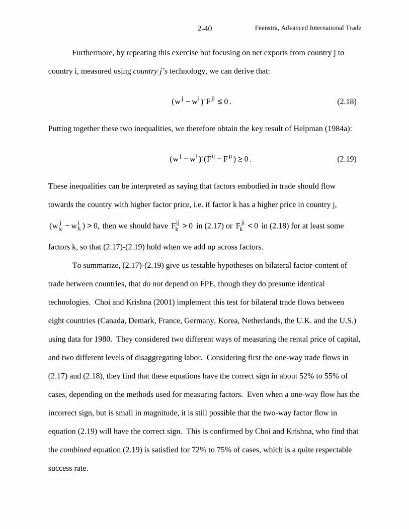
Feenstra, Advanced International Trade2-40
Furthermore, by repeating this exercise but focusing on net exports from country j to
country i, measured using country j’s technology, we can derive that:
0F)'ww( jiij ≤− . (2.18)
Putting together these two inequalities, we therefore obtain the key result of Helpman (1984a):
0)FF()'ww( jiijij ≥−− . (2.19)
These inequalities can be interpreted as saying that factors embodied in trade should flow
towards the country with higher factor price, i.e. if factor k has a higher price in country j,
,0)ww( ik
jk >− then we should have 0Fij
k > in (2.17) or 0F jik < in (2.18) for at least some
factors k, so that (2.17)-(2.19) hold when we add up across factors.
To summarize, (2.17)-(2.19) give us testable hypotheses on bilateral factor-content of
trade between countries, that do not depend on FPE, though they do presume identical
technologies. Choi and Krishna (2001) implement this test for bilateral trade flows between
eight countries (Canada, Demark, France, Germany, Korea, Netherlands, the U.K. and the U.S.)
using data for 1980. They considered two different ways of measuring the rental price of capital,
and two different levels of disaggregating labor. Considering first the one-way trade flows in
(2.17) and (2.18), they find that these equations have the correct sign in about 52% to 55% of
cases, depending on the methods used for measuring factors. Even when a one-way flow has the
incorrect sign, but is small in magnitude, it is still possible that the two-way factor flow in
equation (2.19) will have the correct sign. This is confirmed by Choi and Krishna, who find that
the combined equation (2.19) is satisfied for 72% to 75% of cases, which is a quite respectable
success rate.
Feenstra, Advanced International Trade2-41
Choi and Krishna (2001) also show how (2.17) and (2.18) can be generalized to allow for
scalar technological differences across countries, much like in (2.8). In that case, they find that
the one-way trade flows in (2.17) and (2.18) have the correct sign in 55% to 59% of cases, while
the two-way trade flows in (2.19) have the correct sign in 79% of cases. It is somewhat
surprising that correcting for scalar technology differences between countries did not lead to a
greater improvement in the test results, but then again, this correction improved the “sign test”
for Trefler (1995) from 50% to only 62%. Trefler’s acceptance of the scalar productivity
differences as an improvement over the conventional HOV model was based on other criterion,
and in particular, their ability to help explain the “missing trade.” For the bilateral flows
analyzed by Choi and Krishna, the fact that the combined equation (2.19) – emphasized by
Helpman (1984a) – is satisfied in about three-quarters of cases indicates support for the theory,
and suggests that dropping FPE is an important direction for further research.
Conclusions
We started this chapter with the Leontief paradox, and after explaining this away using
the results of Leamer (1980), went on to argue that the complete tests of the HOV model fail
sadly under the conventional assumptions of this model: identical homothetic tastes and
identical technologies with FPE across countries. As we begin to loosen these assumptions, the
model performs better, and when we allow for unlimited differences in productivities of factors
across countries, as in Trefler (1993), then the resulting HOV equations will hold as an identity.
Between these two extremes, Trefler (1995) shows that a parsimonious specification of
technological differences between countries – allowing for a uniform difference with the U.S. –
is still able to greatly improve the fit of the HOV equation. Recent research such as Davis and
Weinstein (2001a), which we review in the next chapter, generalizes these technological
Feenstra, Advanced International Trade2-42
differences and further explains how we account for the differences between the factor content of
trade and relative endowments.
So what is left for further research? While it is dangerous to predict the course of future
research, we can suggest two areas that deserve further attention. First, it is worth making a
distinction between accounting for global trade volumes and testing hypotheses related to trade.
When we attempt to match the right and left-hand sides of the HOV equation, such as by
introducing productivity parameters, we are engaged in an accounting exercise. With enough
free parameters this is bound to lead to equality of the HOV equation, as we found in (2.13)
which uses the actual technologies of each country, but relies on an assumption about exports.
On the other hand, when we test hypotheses such as (2.17)-(2.19) then we are making use of
economic behavior: the GDP function is concave in the factor endowments, leading to (2.17)-
(2.19), if and only if producers economize on factor inputs when their prices rise. There seems
to be a difference between these two approaches, and ordinarily in economics, we are more
interesting in testing economic behavior.
Second, even if we accept that the HOV equation can fit perfectly by allowing for
sufficient differences between technologies across countries, this begs the question: where do
these differences in technology come from? In the original work of Heckscher and Ohlin, they
rejected the technology differences assumed by Ricardo in favor of a world where knowledge
flowed across borders. We have since learned that this assumption of technological similarity
across countries was empirically false at the time they wrote (see Estevadeordal and Taylor,
2000, 2001), as well as in recent years (Trefler, 1993, 1995; Davis and Weinstein, 2001a). So
we are back in the world of Ricardo, where technological differences are a major determinant of
trade patterns. Such differences can hardly be accepted as exogenous, however, and surely must
Feenstra, Advanced International Trade2-43
be explicable based on underlying causes. Increasing returns to scale might be one explanation,
and this has been incorporated into the HOV framework by Antweiler and Trefler (2002) as will
be discussed in chapter 5. Economy-wide increasing returns are also suggested by the literature
on “endogenous growth,” which we will discuss in chapter 10. Beyond this, some recent authors
have argued that geography/climate (Sachs, 2001), or colonial institutions (Acemoglu, et al,
2001), or social capital (Jones and Hall, 1999), or the efficiency with which labor is utilized
(Clark and Feenstra, 2001) must play an important role. Whatever the answer, this issue will no
doubt occupy researchers for some years to come.
Feenstra, Advanced International Trade2-44
Problems
2.1 Suppose that the factor content of trade is zero on the left of equation (2.7). Then solve for
the implied values of the productivities ikπ in one country relative to another.
2.2 An assumption of the Heckscher-Ohlin-Vanek model, as outlined in this chapter, is that
tastes are identical across countries and also homothetic. The latter is an unrealistic assumption
because of Engel’s Law: expenditures on food are a declining share of total income. Following
Hunter and Markusen (1989), we can introduce non-homothetic tastes using a linear expenditure
system. Denoting per-capital consumption of good i in any country j by jid , we suppose that the
utility function is given by:
∏=
φ−=N
1ii
ji
j i)dd(U , with ∑=
=φN
1ii 1.
The parameters id > 0 in the utility function are interpreted as the “minimum consumption” of
each commodity i=1,…,N. They are assumed to the be the same across countries, as are the
parameters φi > 0.
(a) Assuming that per-capita income jI is large enough to afford the “minimum consumption”,
then show that per-capita demand for each commodity in country j is given by:
ijM
1j jj
iiji p/)dpI(dd ∑ =−φ+= ,
where pj , j=1,…,N, are the commodity prices.
(b) Assuming that prices are the same across countries due to free trade, we can normalize them
at unity, and rewrite demand in the more compact form,
Feenstra, Advanced International Trade2-45
jii
ji Id φ+δ= ,
where )dd(M
1j jiii ∑ =φ−≡δ are the values of “minimum consumption” measured relative to
their mean. Interpret the coefficients δi.
(c) Multiply the per-capita demand by country population jL , to obtain total demand,
ji
ji
ji
jji ELdLD φ+δ== , where jjj ILE ≡ denotes total expenditure in country j. We can write
this in vector notation as, jjj ELD φ+δ= . Using this demand function, re-derive the HOV
equation (2.1), and interpret the new equation.
Feenstra, Advanced International Trade2-46
Empirical Exercises
In these exercises, you will reproduce some of the empirical results from Trefler (1993, 1995).
To complete the exercise, the Excel file “hov_pub.csv” should be stored in the directory:
c:\Empirical_Exercise\Chapter_2\hov_pub.csv. After this, run the STATA program
“hov_pub.do”, which will create a new STATA data file “trefler.dta”. Then do:
2.1 Given identical technologies across countries, run the program “sign_rank_1.do” to conduct
the sign test, rank test, and test for missing trade. Use the results in “sign_rank_1.log” to
replicate columns (2) and (4) in Table 2.5.
2.2 Given uniform technological differences across countries, run the program “sign_rank_2.do”
to redo the sign test, rank test, and missing trade. Use the results in “sign_rank_2.log” to
replicate column (3) and (5), given column (6) in Table 2.5.
2.3 Allowing all factors in each country to have different productivities, now run the program
“compute_pi.do” to compute factor productivities ikπ as Trefler (1993). Note that there are 9
factors in the original data set, but these are now aggregated to just 4 factors, which are labor
(endowment 1), capital (endowment 2), cropland (endowment 3) and pasture (endowment 4).
Using the results in “pi.log” or alternatively in the data files “pi_1.dta, pi_2.dta, pi_3.dta,
pi_4.data” to answer the following:
(a) Which factor has the most negative productivities estimated?
(b) What is the correlation between the estimated labor productivity and the productivities of
other factors? What is the correlation between each factor productivity and GDP per-capita
(which you can find in the file “trefler.dta”)?
Feenstra, Advanced International Trade
Chapter 3: Many Goods and Factors
The Heckscher-Ohlin-Vanek (HOV) model we studied in the previous chapter allowed
for many goods and factors, but for much of that discussion we maintained the assumption of
factor price equalization. This theorem was proved in chapter 1 only for the case of two goods
and two factors (and no factor intensity reversals). A natural question to ask is with many goods
and factors, will factor price equalization continue to hold? More generally, what happens to the
other theorems we discussed in chapter 1 – the Stolper-Samuelson and Rybczynski Theorems?
Are there some generalizations of these that apply to the many good and many factor case?
These are the topics we shall address in this chapter.
We begin with the case where the number of goods and factors is the same, the so-called
“even” case. We will see that the factor price equalization theorem naturally generalizes from
the case of two goods and two factors to N goods and N factors. Versions of the Stolper-
Samuelson and Rybczynski Theorems also continue to hold, though not quite as strong as we
obtained in the two-by-two case.
Then we turn to “uneven” cases, beginning with two goods and three factors. We can
think of the factors as labor, which is mobile between both industries, and a specific factor in
each industry, such as capital or land, which does not move between them. This is the so-called
“specific factors” or Ricardo-Viner model. It will become immediately clear that factor price
equalization does not hold, but rather, that factor prices prevailing in a country depend on its
factor endowments. The results of the Stolper-Samuelson and Rybczynski Theorems are also
modified, depending on whether we are considering a change in the mobile factor (labor) or the
specific factors. The results we obtain for this case illustrate those that apply whenever there are
more factors than goods.
Feenstra, Advanced International Trade3-2
Empirically, the case of an equal number of goods and factors or more factors than goods
can be neatly analyzed using a country’s GDP function. We discuss how these functions can be
estimated using data on a set of industries over time. These techniques have been pioneered by
Diewert (1974) and applied in an international context by Kohli (1978, 1991), Woodland (1982)
and others.1 Harrigan (1997) provides an application to the OECD (Organization for Economic
Cooperation and Development) countries that we shall review, whereby the output shares of
various industries are related to country prices, productivity and factor endowments. By
estimating these share equations, we can then compute the effect of endowment changes on
output shares, namely, the Rybczynski effects. This methodology allows us to explain the
specialization of countries across various industries. In addition, the GDP function allows us to
estimate the dual Stolper-Samuelson effects, as we shall discuss in this chapter and the next.
Finally, we consider the case of more goods than factors, starting with three goods and
two factors. Using the results of Dixit and Norman (1980), we argue that there is a wide range of
possible factor endowments across countries such that factor price equalization continues to
hold, provided that technologies are the same across countries. However, the amount of
production occurring in each country is indeterminate when factor prices are equalized. A test
for production indeterminacy has been implemented by Bernstein and Weinstein (2002), as we
review.2 An elegant generalization of the case with more goods than factor is when there is a
continuum of goods, as in Dornbusch, Fischer and Samuelson (1980). This model allows us to
complete our presentation of empirical results from Davis and Weinstein (2001a) that we
introduced in the last chapter.
1 Burgess (1974a,b, 1976) provides estimates of an aggregate cost rather than GDP function for the U.S., as weshall discuss.2 The empirical methods discussed in this chapter draw upon the survey by Harrigan (2003).
Feenstra, Advanced International Trade3-3
Equilibrium Conditions
We will suppose that there are i=1,…,N goods, and j=1,…,M factors. The production
functions are written )v(fy iii = , where vi = (vi1,…,viM) is the vector of factor inputs. As usual
we assume that the production functions are positive, increasing, concave and homogeneous of
degree one for all vi > 0. Denoting the vector of factor prices by w, the unit-cost functions are
ci(w) ≡ }1)v(f|v'w{min iii0vi
≥≥
, which are also positive, increasing, concave and homogeneous of
degree one for all w > 0. The zero profit conditions are then stated as:
)w(cp ii = , i=1,…,N. (3.1)
The second set of equilibrium conditions is full-employment of resources. As in chapter
1, we write )w(aw/c ii =∂∂ as the amount of factors used for one unit of production, and it
follows that the total inputs used in industry i are vi = yi ai(w). We denote the elements of the
vector ai(w) by aij(w), j=1,…,M. Then the full-employment conditions are stated as:
jiij
N
1iVy)w(a =∑
=, j=1,…,M, (3.2)
where Vj is the endowment of resource j. In matrix notation, let A =[a1(w)',…, aM(w)'] denote
the MxN matrix of primary factors needed for one unit of production in each industry, where the
columns of this matrix measure the different industries i=1,…,N. The full-employment
conditions (3.2) are then written compactly as:
AY = V, (3.2’)
Feenstra, Advanced International Trade3-4
where Y is the (Nx1) vector of output and V is the (Mx1) vector of factor endowments.
The equilibrium conditions (3.1) and (3.2) are N+M equations in N+M unknowns,
namely, the factor prices wj, j=1,…,M and outputs yi, i=1,…,N. To analyze these, it will be
helpful to use the GDP function for the economy, which is defined as:
G(p,V) ∑∑==≥
≤≡N
1ii
N
1iiii
0vVvtosubject)v(fpmax
i
, (3.3)
where p = (p1,…,pN) and V = (V1,…,VM) are the price and endowment vectors. To solve this
maximization problem, we substitute the constraint (written with equality) into the objective
function, and write the output of good 1 as ( )∑ =− N2i i1 vVf , so that the maximized value of GDP
becomes, G(p,V) = ( ) ∑∑ == +− N2i iii
N2i i11 )v(fpvVfp . From the envelope theorem, we can
differentiate this with respect to p and V while holding the optimal inputs choices vi fixed,
i=2,…,N. Then we obtain:
(a) ∂G/∂pi = fi(vi) = yi , which is the output of industry i;
(b) ∂G/∂Vj = p1∂f1/∂vij , which is the factor price wj .
Furthermore, by Young’s theorem we know that, ∂2G/∂pi∂Vj = ∂2
G/∂Vj∂pi, so it follows that:
(c)j
i
ij
2
i
j
ji
2
dV
dy
pV
G
dp
dw
Vp
G =∂∂
∂==∂∂
∂. (3.4)
Feenstra, Advanced International Trade3-5
Samuelson (1953-54) called conditions (3.4) the “reciprocity relations,” and it shows that the
Stolper-Samuelson derivatives are identical to the Rybczynski derivatives! Results (a)-(c) hold
regardless of the number of goods and factors, but require differentiability of the GDP function.
We shall comment on the validity of this assumption below.
We now consider some special cases.
Same Number of Goods and Factors
With N=M, the zero-profit conditions (3.1) become N equations in N unknowns. The
question, then, is whether we can obtain a solution for the wages w and if this solution is unique.
In chapter 1, we discussed the case of “factor intensity reversals,” whereby the iso-cost lines of
the unit-costs curves for two industries intersect twice (see Figure 1.6). This means that there are
some prices for the two industries such that the iso-cost lines are tangent, as shown in Figure 3.1
at point B. At these factor prices, the factor requirements vectors ai(w) in the two industries are
proportional.
A factor intensity reversal (FIR) means that there are factor prices w at which two
columns of the matrix A are proportional, so that A is singular. Actually, a factor intensity
reversal occurs even if the components of a1(w) and a2(w) for just two factors are proportional,
i.e. point B in Figure 3.1 holds for factors 1 and 2, even though the demand for the other factors
in these industries are not proportional. To rule out this case, we therefore require a stricter
assumption than the nonsingularity of A.
Samuelson (1953-54) first proposed the condition that the leading principle minors of A
are all non-negative, i.e.,
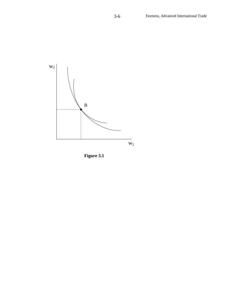
Feenstra, Advanced International Trade3-6
B
w1
w2
Figure 3.1
Feenstra, Advanced International Trade3-7
0
aa
aa
,...,0aa
aa,0a
NNN1
1N11
2212
211111 ≠≠≠
L
MOM
L
. (3.5)
By a natural re-ordering of the goods and factors, the signs of all these determinants can be taken
as positive. However, Nikaido (1972) showed that this condition was not enough to ensure that
the system of equations (3.1) has a unique solution for w given any p > 0. Instead, it had to be
strengthened as: there exist bounds b > 0 and B > 0 such that,
B
aa
aa
,...,aa
aa,ab0
NNN1
1N11
2212
211111 ≤≤<
L
MOM
L
. (3.6)
Then we have the following “factor price insensitivity” result, as named by Leamer (1995):
Lemma (Samuelson, 1953-54; Nikaido, 1972)
Assume N=M and that condition (3.6) holds for all w > 0. Then for all p > 0, the set of equations
(3.1) has a unique solution for factor prices w > 0.
This Lemma implies that the factor prices can be written as a function of product prices,
or w(p), independent of endowments. Note that this implies a special form for the GDP function
(3.3). With constant returns to scale in all industries, GDP can be written in general as G(p,V) =
∑ =M
1j jj V)V,p(w , which is just the sum of payment to primary factors. Under the conditions of
the above Lemma, this formula is simplified to:
G(p,V) = ∑ =M
1j jj V)p(w . (3.7)
Feenstra, Advanced International Trade3-8
In particular, this implies that ∂2G/∂Vj∂Vi = 0, so there are no diminishing returns to the
accumulation of a factor in the economy overall.
Now suppose that two countries share the same technologies, and therefore the same unit-
cost functions, and through free trade they face the same prices p. Provided that both countries
are producing all i=1,…,N goods, then this Lemma establishes that they will have the same
factor prices, so factor price equalization (FPE) is obtained. The set of endowments that allow
both countries to be producing yi > 0 for i=1,…,N, can be computed from the full-employment
conditions (3.2). This will be an FPE set, analogous to Figure 1.9 in chapter 1. In the case of
equal goods and factors, the FPE set is a higher-dimension analogue to Figure 1.9: rather than a
parallelogram in 2 dimensions, we would have a hyper-parallelogram in N dimensions. So for
factor-price equalization, the extension from 2 goods and 2 factors to N goods and N factors is
obtained quite easily.
What about the Stolper-Samuelson and Rybczyski Theorems? To see what sort of
generalization can be obtained for these, let us totally differentiate the zero-profit conditions
(3.1), and apply the Jones’ (1965) algebra, to obtain:
jij
M
1ji wp θ=∑
=, i=1,…,M, (3.8)
where θij = wjaij/ci denotes the cost-share of factor j in industry i. As we saw in chapter 1, the
changes in commodity prices are weighted averages of the changes in factor prices. For a
change in the price of each commodity i, holding other goods prices fixed, there must then exist
factors j and k such that ij pw ≥ and 0wk ≤ . Under additional conditions we can establish that
Feenstra, Advanced International Trade3-9
these inequalities are strict,3 and therefore, factor j has gained in real terms and factor k has lost
in real terms. The Stolper-Samuelson Theorem generalizes in this sense: for a change in the
price of each good, there will exist some factor that gains in real terms and another that loses.
A similar generalization holds for the Rybczynski Theorem. To see this, differentiate the
full-employment conditions (3.2) with respect to endowment Vk, holding prices (and therefore
factor prices) fixed, obtaining:
0)w(adV
dyij
N
1i k
i =∑=
, j=1,…,M, j≠k, (3.9a)
1)w(adV
dyik
N
1i k
i =∑=
. (3.9b)
Provided that the matrix A is nonsingular at the prevailing factor prices, then we can use the
conditions (3.9) to uniquely determine the Rybczynski derivatives ki dV/dy . From condition
(3.9b), it must be the case that 0dV/dy ki > for some good i. Using this in (3.9a), there must
exist some other good j for which 0dV/dy kj < . Thus, we have shown that for an increase in
the endowment of each factor, there must be a good whose output rises and another good whose
output falls.
This generalization of the Rybczynski Theorem is fine, but our results for the Stolper-
Samuelson Theorem are not fully satisfactory. Recall that in the two-by-two model, labor and
capital each suffer from an increase in the price of some good. Does this apply in the NxN case?
Jones and Scheinkman (1977) answer this in the affirmative:
3 Either (1974, 1984) assumed that aij > 0 for all factors and industries. Jones and Scheinkman (1977, p. 929) usethe weaker assumption that every industry employs at least two inputs, and each input is employed in at least twoindustries. However, they both assume that with a small change in prices every good is still produced. This means
that the factor intensities aij cannot be proportional in two industries.
Feenstra, Advanced International Trade3-10
Theorem (Jones and Scheinkman, 1977)
Assume that N=M, and that the matrix A is nonsingular at the prevailing factor prices. Then for
each factor, there must be a good such that an increase in the price of that good will lower the
real return to the factor.
The proof of this theorem follows from (3.9) and the reciprocity relations (3.4): starting
with any factor k, we know that 0dV/dy kj < for some good j, and so it follows that
0dp/dw jk < for some good j. Since all other prices are fixed, it follows that wk/pi has fallen,
along with wk/pj, i≠j, so that the real return to factor j has been reduced. Jones and Scheinkman
interpret this theorem as saying that “each factor has a good that is a natural enemy,” in the sense
that raising the price of that good will lower the return to the factor. However, in the general
case of N=M > 2 goods and factors, we cannot prove in general that “each factor has a good that
is a natural friend;” i.e., for each factor, there need not exist a good such that increasing the price
of that good will raise the real return to the factor.4 We have already argued that raising a price
will increase the real return to some factor, but we cannot establish that each factor will benefit
in real terms due to an increase in the price of some good. So factors have “natural enemies” but
not necessarily “natural friends.”
Empirical estimates of the Rybczynski effects in the “even” case have already been
shown in the previous chapter, from Leamer (1984). Harrigan (1995) re-examines a similar set
of regressions but using industry outputs as the dependent variable rather than net trade. The
explanatory variables are country factor endowments, and the linear relationship between outputs
4 Either (1984, Proposition 20) argues that there will be a “qualified” friend, in the sense that raising somecommodity price will raise that factor price enough to lower the aggregate income of all other factors.
Feenstra, Advanced International Trade3-11
and factor endowments follows directly from inverting (3.2’), obtaining Y = A-1V, or:
∑=
β=M
1k
ikjk
ij Vy , i = 1,…,C; j = 1,…,N, (3.10)
where i now indexes countries, j indexes goods, k indexes factors, and βjk denotes the elements
of A-1
. Harrigan uses data for the OECD countries over 1970-1985 for 10 manufacturing sectors
and four factor supplies: capital, skilled and unskilled labor, and land. Notice that the number of
goods exceeds the number of factors in this formulation, even though inverting (3.2’) assumes
that N=M. We can think of Harrigan’s approach as assuming N=M in terms of the “true”
number of goods and factors, but then aggregating factors in the data so that there are only four.
More generally, this discussion points out that whether or not there is an equal number of goods
and factors cannot be judged by simply “counting” these: instead, we would need to test some
hypotheses to determine this, as we shall discuss in the sections that follow.
The results obtained by regressing industry outputs on factor endowments, over the panel
of OECD countries and years, are similar to those obtained by Leamer (1984): for each
manufacturing industry there is at least one factor with a negative Rybczynski effect, indicating
that an increase in that endowment would reduce the manufacturing output. These factors were
usually skilled or unskilled labor, and sometimes land. Conversely, capital has a positive
coefficient βjk in all ten regressions, indicating that an increase in this endowment will raise
manufacturing output. Beyond these results, Harrigan (1995) is able to explore properties of the
panel dataset which Leamer (1984) could not since he only had data for two years. Harrigan
finds that fixed effects for countries are very important, indicating that there are systematic
differences across countries not captured by the theory underlying (3.10). The most significant
Feenstra, Advanced International Trade3-12
assumption in applying (3.10) to panel data is that technologies are the same across countries
and time. We will be eliminating this assumption later in this chapter.
More Factors than Goods
We turn now to the case of more factors than goods, M > N. We can again differentiate
the zero-profit conditions to obtain (3.8), so our generalization of the Stolper-Samuelson
Theorem continues to hold: an increase in the price of each good will lead to a rise in the real
return to some factor, and a fall in the real return to another. However, our generalization of the
Rybczynski Theorem does not hold: when we differentiate the full-employment conditions we
do not obtain (3.9), because now a change in factor endowments leads to a change in their prices,
so the factor-intensities aij will change. Furthermore, the fact that (3.9) does not hold means that
the theorem due to Jones and Scheinkman (1977) will not hold either: it is no longer that case
that each factor has a good that is a “natural enemy.”
To illustrate these results, we focus on the special case of two goods and three factors, in
what is called the “specific factors” or the Ricardo-Viner model. This model has been analyzed
by Jones (1971), Mayer (1974), Mussa (1974), and Neary (1978), among others. Let us return to
the notation that the two sectors use labor and capital, with production functions yi = fi(Li , Ki).
We now assume that the capital stocks Ki are fixed in each industry, so that labor is the only
factor that moves between them. This framework is sometimes viewed as a “short run” version
of the Heckscher-Ohlin model, for a time span short enough such that capital is fixed.
The full employment condition for labor is L1 + L2 < L, and so the GDP function for the
sector-specific economy is:
Feenstra, Advanced International Trade3-13
G(p,L,K1,K2) LLLtosubject)K,L(fpmax 21
2
1iiiii
0Li
≤+≡ ∑=≥
. (3.11)
To maximize GDP, labor will flow between the two industries until its marginal value product is
the same in each. This first-order condition is stated as,
)K,L(fp)K,L(fpwL
G22L2211L11 ===
∂∂
. (3.12)
With the capital stocks fixed, (3.12) is easily solved for the labor allocation, as is illustrated in
Figure 3.2. The horizontal axis measures the total labor endowment L, which is allocated
between industry 1 (measured from its origin 01) and industry 2 (measured from its origin 02).
Concavity of the production functions implies a diminishing marginal product of labor, so both
curves pifiL are drawn as downward sloping relative to their origins. The equilibrium wage is
determined at the intersection of these two curves, point A.
Note that the position of the marginal product curves depends on the amount of capital in
each industry, and therefore, so does the equilibrium wage at point A. Thus, with two countries
having the same technology and facing the same prices due to free trade, but with differing
endowments, there will not be factor price equalization: rather, the price of each factor will be
inversely related to their endowments.5
Now suppose that there is an exogenous increase in the price of good 1. What is the
effect on factor prices? In Figure 3.3, the marginal value product curve of industry 1 will shift
up by ∆p1f1L, as illustrated. It is immediate that the wage increases along with the allocation of
labor to industry 1. From (3.12), we can compute the increase in the wage as:
5 See problem 3.1.
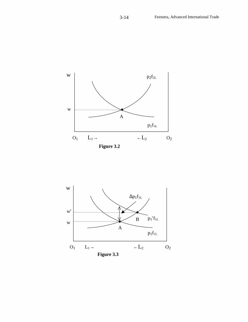
Feenstra, Advanced International Trade3-14
B
Ap1f1L
p1′f1L
O1 L1→ ←L2 O2
w
w′
w
∆p1f1L
Figure 3.3
A
p1f1L
O1 L1→ ←L2 O2
w
w
p2f2L
Figure 3.2
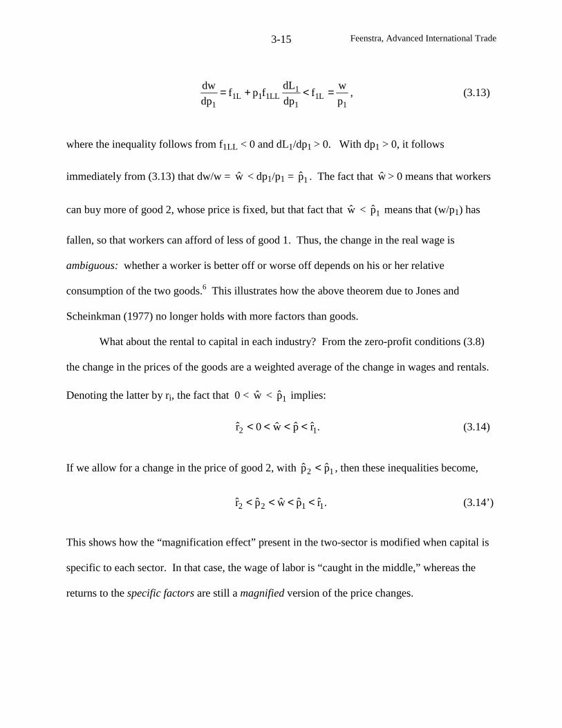
Feenstra, Advanced International Trade3-15
1L1
1
1LL11L1
1 p
wf
dp
dLfpf
dp
dw =<+= , (3.13)
where the inequality follows from f1LL < 0 and dL1/dp1 > 0. With dp1 > 0, it follows
immediately from (3.13) that dw/w = w < dp1/p1 = 1p . The fact that w > 0 means that workers
can buy more of good 2, whose price is fixed, but that fact that w < 1p means that (w/p1) has
fallen, so that workers can afford of less of good 1. Thus, the change in the real wage is
ambiguous: whether a worker is better off or worse off depends on his or her relative
consumption of the two goods.6 This illustrates how the above theorem due to Jones and
Scheinkman (1977) no longer holds with more factors than goods.
What about the rental to capital in each industry? From the zero-profit conditions (3.8)
the change in the prices of the goods are a weighted average of the change in wages and rentals.
Denoting the latter by ri, the fact that 0 < w < 1p implies:
.rpw0r 12 <<<< (3.14)
If we allow for a change in the price of good 2, with 12 pp < , then these inequalities become,
.rpwpr 1122 <<<< (3.14’)
This shows how the “magnification effect” present in the two-sector is modified when capital is
specific to each sector. In that case, the wage of labor is “caught in the middle,” whereas the
returns to the specific factors are still a magnified version of the price changes.
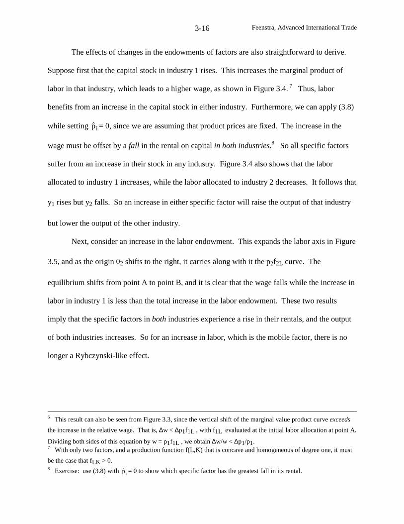
Feenstra, Advanced International Trade3-16
The effects of changes in the endowments of factors are also straightforward to derive.
Suppose first that the capital stock in industry 1 rises. This increases the marginal product of
labor in that industry, which leads to a higher wage, as shown in Figure 3.4. 7 Thus, labor
benefits from an increase in the capital stock in either industry. Furthermore, we can apply (3.8)
while setting ip = 0, since we are assuming that product prices are fixed. The increase in the
wage must be offset by a fall in the rental on capital in both industries.8 So all specific factors
suffer from an increase in their stock in any industry. Figure 3.4 also shows that the labor
allocated to industry 1 increases, while the labor allocated to industry 2 decreases. It follows that
y1 rises but y2 falls. So an increase in either specific factor will raise the output of that industry
but lower the output of the other industry.
Next, consider an increase in the labor endowment. This expands the labor axis in Figure
3.5, and as the origin 02 shifts to the right, it carries along with it the p2f2L curve. The
equilibrium shifts from point A to point B, and it is clear that the wage falls while the increase in
labor in industry 1 is less than the total increase in the labor endowment. These two results
imply that the specific factors in both industries experience a rise in their rentals, and the output
of both industries increases. So for an increase in labor, which is the mobile factor, there is no
longer a Rybczynski-like effect.
6 This result can also be seen from Figure 3.3, since the vertical shift of the marginal value product curve exceeds
the increase in the relative wage. That is, ∆w < ∆p1f1L , with f1L evaluated at the initial labor allocation at point A.
Dividing both sides of this equation by w = p1f1L , we obtain ∆w/w < ∆p1/p1.7 With only two factors, and a production function f(L,K) that is concave and homogeneous of degree one, it must
be the case that fLK > 0.8 Exercise: use (3.8) with ip = 0 to show which specific factor has the greatest fall in its rental.
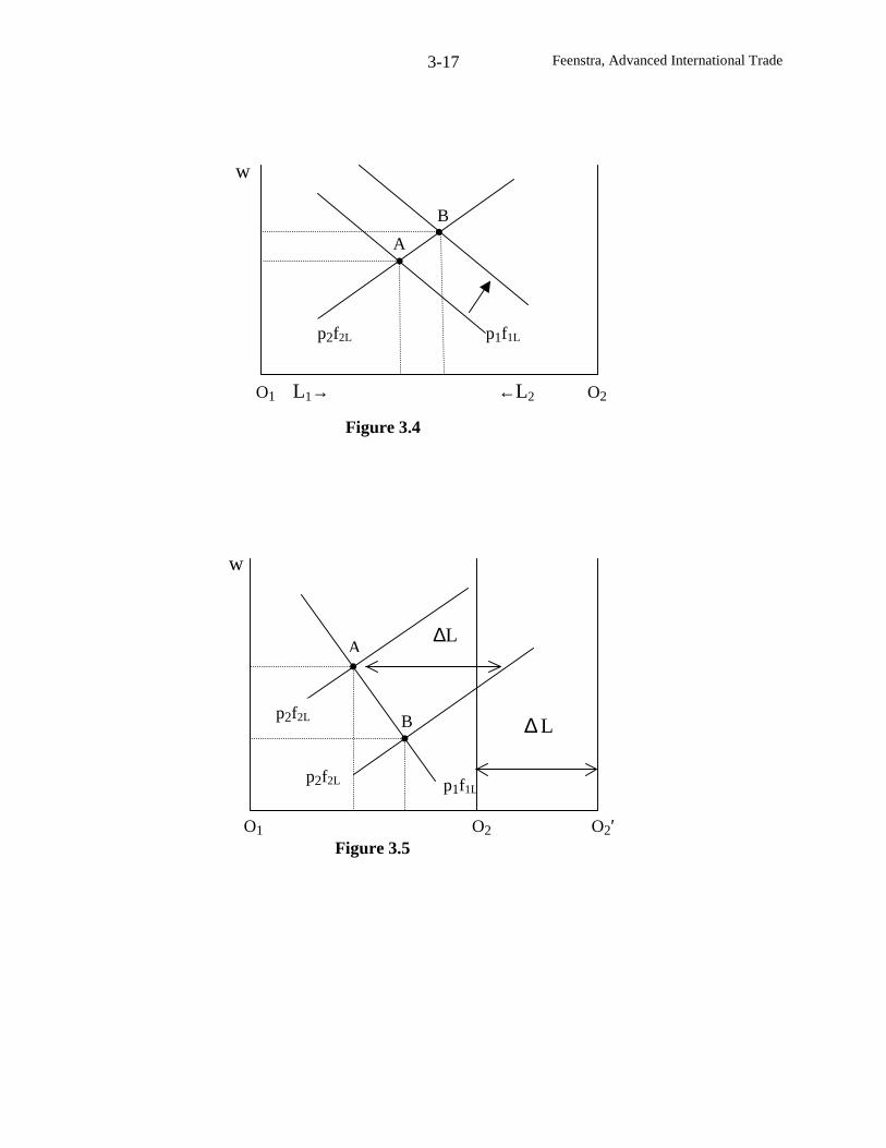
Feenstra, Advanced International Trade3-17
B
A
p2f2L p1f1L
w
O1 L1→ ←L2 O2
Figure 3.4
L∆
L∆
w
p1f1L
O1 O2 O2′Figure 3.5
A
Bp2f2L
p2f2L
Feenstra, Advanced International Trade3-18
Estimating the GDP Function
The number of goods and factors, as well as whether factors are mobile or not, all
influence the form of the GDP function. To capture these effects empirically we can hypothesize
a very general functional form for GDP and then use data on industry output and prices, as well
as factor endowments and prices, to estimate the GDP function. By taking the derivatives of the
estimated GDP function with respect to prices and factor endowments, we can then obtain the
Rybczynski and Stolper-Samuelson derivatives that apply to an actual economy.
The first step is to choose a functional form for GDP. A convenient choice is the translog
function, which was introduced by Diewert (1974, p. 139) and initially used in the international
trade literature by Kohli (1978). This function is written as,
k
N
1i
M
1kiik
M
1k
M
1kk2
1
j
N
1i
N
1jiij
N
1i
M
1k2
1kkii0
VlnplnVlnVln
plnplnVlnplnGln
∑ ∑∑∑
∑∑∑ ∑
= == =
= == =
φ+δ+
γ+β+α+α=
ll
l
(3.15)
where pi denotes the prices of products i=1,…,N, and Vk denotes the endowments of factors
k=1,…,M. In order to ensure that the translog GDP function is homogeneous of degree one in
prices, we impose the requirements,9
.0and1N
1iik
N
1iij
N
1ii =φ=γ=α ∑∑∑
===(3.16)
In addition, to ensure that the GDP function is homogeneous of degree one in endowments, we
impose the requirements,
9 Without loss of generality, we also impose the symmetry restrictions γij = γji and lkδ = klδ . See problem 3.2 to
show that (3.16) and symmetry ensures that the translog cost function is homogeneous of degree one in prices.
Feenstra, Advanced International Trade3-19
.0and1M
1kik
M
1kk
M
1kk =φ=δ=β ∑∑∑
===l (3.17)
The usefulness of the translog function comes from computing its first derivatives,
∂lnG/∂lnpi = (∂G/∂pi)(pi/G). Because ∂G/∂pi equals the output of sector i, it follows that
(∂G/∂pi)(pi/G) equals the share of sector i in GDP, which we denote by the output-shares
si = piyi/G. Thus, differentiating (3.15) with respect to ln pi we obtain,
k
M
1kik
N
1jjijii Vlnplns ∑∑
==φ+γ+α= , i=1,…,N. (3.18)
In addition, we can compute the first derivatives with respect to factor endowments,
obtaining ∂lnG/∂lnVk = (∂G/∂Vk)(Vk/G). Because ∂G/∂Vk equals the factor price of endowment
k, it follows that (∂G/∂Vk)(Vk/G) equals the share of GDP devoted to factor k, which we denote
by the factor-shares sk = wkVk/G. Thus, differentiating (3.15) with respect to ln Vk we obtain,
i
N
1iik
M
1kkk plnVlns ∑∑
==φ+δ+β=
lll , k=1,…,M. (3.19)
Equations (3.18) and (3.19) are N+M linear equations that can be estimated using annual
data on output and factor shares, product prices, and endowments. The dependent variables in
each of (3.18) and (3.19) sum to unity, which means that one of the equations can be derived
from the others. Under these conditions, one of the equations is dropped from each of (3.18) and
(3.19) before the system is estimated, leaving (N+M-2) equations. With annual observations
over T years, this means that there are (N+M-2)T observations used to estimate the coefficients
Feenstra, Advanced International Trade3-20
γij, φik and lkδ .10 The great advantage of estimating this system of shares equations, rather than
just the GDP function in (3.15), is that there are more observations and degrees of freedom.
Even with just a modest number of annual observations, such as 20, the researcher can expect to
obtain reasonably precise estimates of the coefficients.
The coefficients φik in (3.18) measure the response of each output share to changes in the
endowments, and are referred to as output elasticities. These are similar to the Rybczynski
effects, which are normally defined as the impact of a change in endowments on the level of
output rather than its share. To make this conversion, write the quantity of each output as
)p/Gsln(yln iii = . Differentiating this with respect to an endowment kVln using (3.15) and
(3.18), we obtain the Rybczynski elasticity:
ki
ik
k
i ssVln
yln +φ=∂∂
. (3.20)
Thus, the coefficients φik together with the input and output shares can be used to calculate the
Rybczynski elasticity.
Similarly, write the price of each factor as )V/Gsln(wln kkk = . Differentiating this
with respect to ipln using (3.15) and (3.19), it follows that the Stolper-Samuelson elasticities
are:
ik
ik
i
k sspln
wln +φ=∂∂
. (3.21)
In addition, we can differentiate )V/Gsln(wln kkk = with respect to the factor endowments to
obtain:
10 The hypotheses of symmetry and homogeneity, in (3.16) and (3.17), can be tested by first estimating the translogsystem without these restrictions and comparing the system estimated with the restrictions.
Feenstra, Advanced International Trade3-21
≠+δ
=−+δ
=∂∂
.kif,ss
,kif,1ss
Vln
wln
k
k
kk
kk
k
l
l
lll
(3.22)
These elasticities allow us to test the hypothesis of “factor price insensitivity,” meaning that the
GDP function takes the special form in (3.7). While this functional form cannot be imposed
globally for the translog GDP function, it can be evaluated locally by testing whether (3.22) is
zero. This means that we test )s1(s kkkk −=δ and ll sskk −=δ , which can be performed at one
year (e.g. the midpoint) of the sample. In summary, given the estimated coefficients from the
translog share equations, we can readily compute the Rybczynski and Stolper-Samuelson
elasticities and also test for “factor price insensitivity.”
Turning to empirical applications, Kohli (1978) estimates a translog GDP function for
Canada while Kohli (1990a) estimates it for U.S. data. Focusing on the U.S. application, Kohli
uses the five major GDP components as goods: consumption (C), investment (I), government
services (G), exports (X) and imports (M). Notice that he treats exports and imports as an output
and input, respectively, in the production process. This is quite different from our treatment in
the previous chapter where net exports were the difference between consumption and production:
now we are defining exports and imports independently from consumption. This makes sense if
exports are differentiated from domestic goods and if imports are mainly intermediate inputs.
Both of these are plausible hypotheses, and we will explore the role of imports as intermediate
inputs more in the next chapter.
For primary inputs Kohli (1990a) identifies labor and capital, so he obtains five output-
share equations (3.18) (where imports have a negative share) and two factor-share equations
(3.19). Dropping one equation from each system, we then have five equations in total, and with
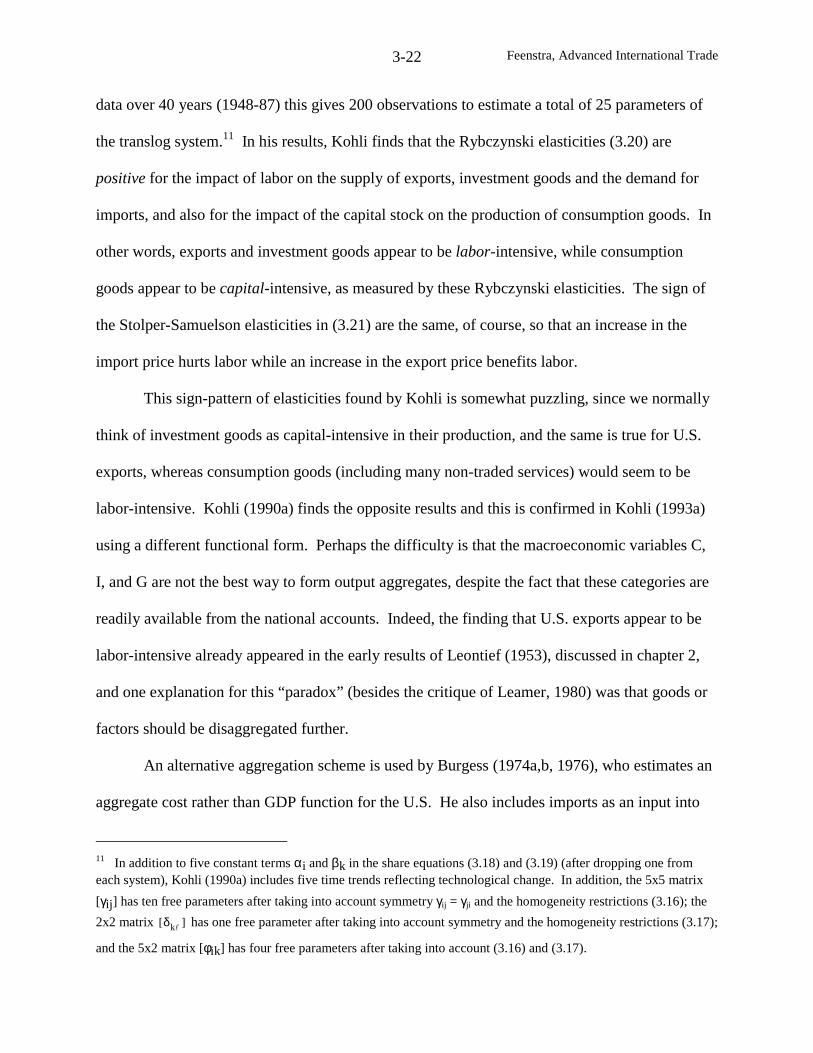
Feenstra, Advanced International Trade3-22
data over 40 years (1948-87) this gives 200 observations to estimate a total of 25 parameters of
the translog system.11 In his results, Kohli finds that the Rybczynski elasticities (3.20) are
positive for the impact of labor on the supply of exports, investment goods and the demand for
imports, and also for the impact of the capital stock on the production of consumption goods. In
other words, exports and investment goods appear to be labor-intensive, while consumption
goods appear to be capital-intensive, as measured by these Rybczynski elasticities. The sign of
the Stolper-Samuelson elasticities in (3.21) are the same, of course, so that an increase in the
import price hurts labor while an increase in the export price benefits labor.
This sign-pattern of elasticities found by Kohli is somewhat puzzling, since we normally
think of investment goods as capital-intensive in their production, and the same is true for U.S.
exports, whereas consumption goods (including many non-traded services) would seem to be
labor-intensive. Kohli (1990a) finds the opposite results and this is confirmed in Kohli (1993a)
using a different functional form. Perhaps the difficulty is that the macroeconomic variables C,
I, and G are not the best way to form output aggregates, despite the fact that these categories are
readily available from the national accounts. Indeed, the finding that U.S. exports appear to be
labor-intensive already appeared in the early results of Leontief (1953), discussed in chapter 2,
and one explanation for this “paradox” (besides the critique of Leamer, 1980) was that goods or
factors should be disaggregated further.
An alternative aggregation scheme is used by Burgess (1974a,b, 1976), who estimates an
aggregate cost rather than GDP function for the U.S. He also includes imports as an input into
11 In addition to five constant terms αi and βk in the share equations (3.18) and (3.19) (after dropping one fromeach system), Kohli (1990a) includes five time trends reflecting technological change. In addition, the 5x5 matrix
[γij] has ten free parameters after taking into account symmetry γij = γji and the homogeneity restrictions (3.16); the
2x2 matrix ][ klδ has one free parameter after taking into account symmetry and the homogeneity restrictions (3.17);
and the 5x2 matrix [φik] has four free parameters after taking into account (3.16) and (3.17).
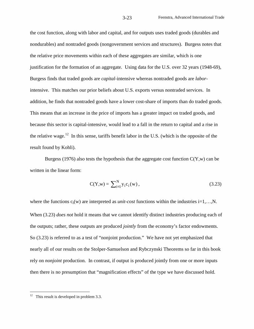
Feenstra, Advanced International Trade3-23
the cost function, along with labor and capital, and for outputs uses traded goods (durables and
nondurables) and nontraded goods (nongovernment services and structures). Burgess notes that
the relative price movements within each of these aggregates are similar, which is one
justification for the formation of an aggregate. Using data for the U.S. over 32 years (1948-69),
Burgess finds that traded goods are capital-intensive whereas nontraded goods are labor-
intensive. This matches our prior beliefs about U.S. exports versus nontraded services. In
addition, he finds that nontraded goods have a lower cost-share of imports than do traded goods.
This means that an increase in the price of imports has a greater impact on traded goods, and
because this sector is capital-intensive, would lead to a fall in the return to capital and a rise in
the relative wage.12 In this sense, tariffs benefit labor in the U.S. (which is the opposite of the
result found by Kohli).
Burgess (1976) also tests the hypothesis that the aggregate cost function C(Y,w) can be
written in the linear form:
C(Y,w) = ∑ =N
1i ii )w(cy , (3.23)
where the functions ci(w) are interpreted as unit-cost functions within the industries i=1,…,N.
When (3.23) does not hold it means that we cannot identify distinct industries producing each of
the outputs; rather, these outputs are produced jointly from the economy’s factor endowments.
So (3.23) is referred to as a test of “nonjoint production.” We have not yet emphasized that
nearly all of our results on the Stolper-Samuelson and Rybczynski Theorems so far in this book
rely on nonjoint production. In contrast, if output is produced jointly from one or more inputs
then there is no presumption that “magnification effects” of the type we have discussed hold.
12 This result is developed in problem 3.3.
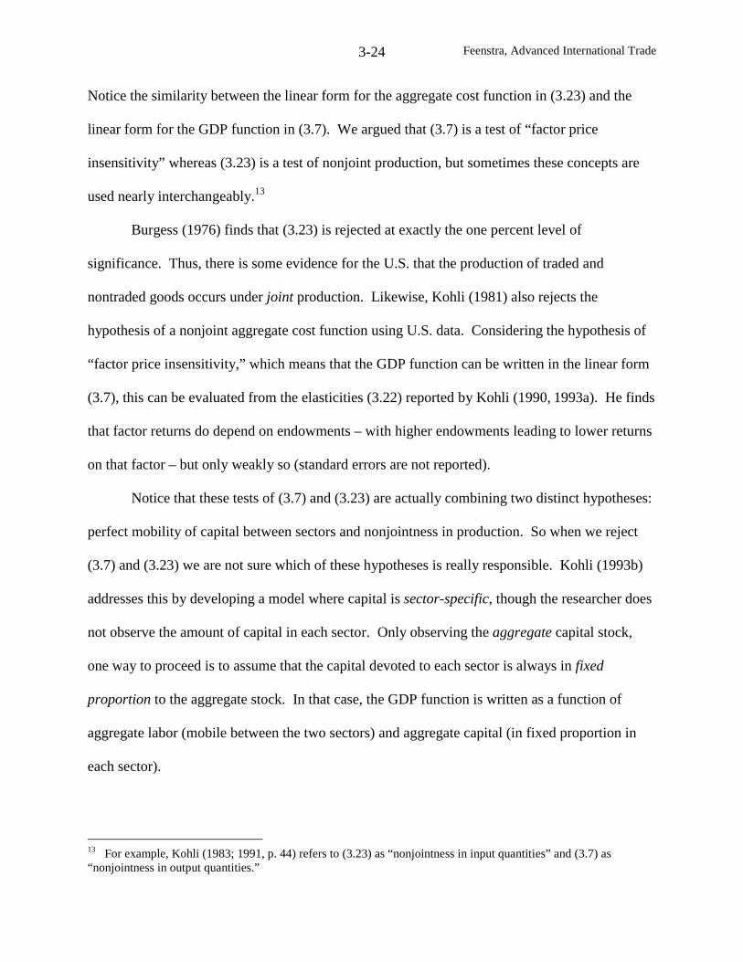
Feenstra, Advanced International Trade3-24
Notice the similarity between the linear form for the aggregate cost function in (3.23) and the
linear form for the GDP function in (3.7). We argued that (3.7) is a test of “factor price
insensitivity” whereas (3.23) is a test of nonjoint production, but sometimes these concepts are
used nearly interchangeably.13
Burgess (1976) finds that (3.23) is rejected at exactly the one percent level of
significance. Thus, there is some evidence for the U.S. that the production of traded and
nontraded goods occurs under joint production. Likewise, Kohli (1981) also rejects the
hypothesis of a nonjoint aggregate cost function using U.S. data. Considering the hypothesis of
“factor price insensitivity,” which means that the GDP function can be written in the linear form
(3.7), this can be evaluated from the elasticities (3.22) reported by Kohli (1990, 1993a). He finds
that factor returns do depend on endowments – with higher endowments leading to lower returns
on that factor – but only weakly so (standard errors are not reported).
Notice that these tests of (3.7) and (3.23) are actually combining two distinct hypotheses:
perfect mobility of capital between sectors and nonjointness in production. So when we reject
(3.7) and (3.23) we are not sure which of these hypotheses is really responsible. Kohli (1993b)
addresses this by developing a model where capital is sector-specific, though the researcher does
not observe the amount of capital in each sector. Only observing the aggregate capital stock,
one way to proceed is to assume that the capital devoted to each sector is always in fixed
proportion to the aggregate stock. In that case, the GDP function is written as a function of
aggregate labor (mobile between the two sectors) and aggregate capital (in fixed proportion in
each sector).
13 For example, Kohli (1983; 1991, p. 44) refers to (3.23) as “nonjointness in input quantities” and (3.7) as“nonjointness in output quantities.”
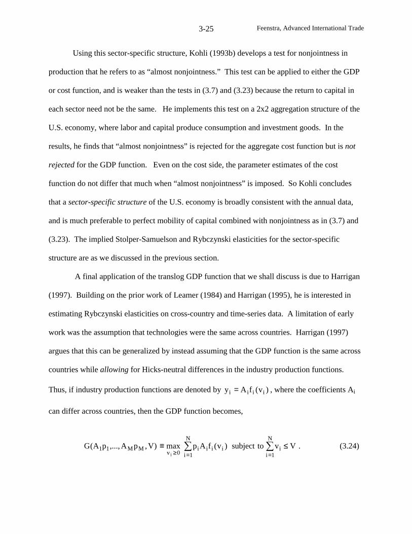
Feenstra, Advanced International Trade3-25
Using this sector-specific structure, Kohli (1993b) develops a test for nonjointness in
production that he refers to as “almost nonjointness.” This test can be applied to either the GDP
or cost function, and is weaker than the tests in (3.7) and (3.23) because the return to capital in
each sector need not be the same. He implements this test on a 2x2 aggregation structure of the
U.S. economy, where labor and capital produce consumption and investment goods. In the
results, he finds that “almost nonjointness” is rejected for the aggregate cost function but is not
rejected for the GDP function. Even on the cost side, the parameter estimates of the cost
function do not differ that much when “almost nonjointness” is imposed. So Kohli concludes
that a sector-specific structure of the U.S. economy is broadly consistent with the annual data,
and is much preferable to perfect mobility of capital combined with nonjointness as in (3.7) and
(3.23). The implied Stolper-Samuelson and Rybczynski elasticities for the sector-specific
structure are as we discussed in the previous section.
A final application of the translog GDP function that we shall discuss is due to Harrigan
(1997). Building on the prior work of Leamer (1984) and Harrigan (1995), he is interested in
estimating Rybczynski elasticities on cross-country and time-series data. A limitation of early
work was the assumption that technologies were the same across countries. Harrigan (1997)
argues that this can be generalized by instead assuming that the GDP function is the same across
countries while allowing for Hicks-neutral differences in the industry production functions.
Thus, if industry production functions are denoted by )v(fAy iiii = , where the coefficients Ai
can differ across countries, then the GDP function becomes,
)V,pA,...,pA(G MM11 ∑∑==≥
≤≡N
1ii
N
1iiiii
0vVvtosubject)v(fApmax
i
. (3.24)
Feenstra, Advanced International Trade3-26
Notice that we have multiplied the prices pi appearing in the GDP function by the Hick’s-neutral
productivity parameters Ai, because that is how they appear on the right of (3.24). If we adopt a
translog form for the GDP function, then the output-share equations in (3.18) would be
written as:
k
M
1kik
N
1jjjijii Vln)pAln(s ∑∑
==φ+γ+α= , i=1,…,N. (3.25)
That is, the output-shares of each industry depend on their prices and productivities (with the
same coefficient applying to each), as well as the factor endowments.
We will be discussing the measurement of industry productivity further in chapters 4 and
10, as well as properties of the GDP function in (3.24). For the present purposes, we note that
Harrigan (1997) assumes that countries are engaged in free trade so that industry prices are the
same, and no longer appear in (3.25):14 it follows that the determinants of the output-shares are
productivities and endowments. It is the inclusion of the productivity variables in (3.25) that
distinguishes this approach from Leamer (1984) and Harrigan (1995) and this is an important
generalization from earlier research.15
Harrigan estimates (3.25) over a panel data set consisting of 10 OECD countries over
about 20 years (from 1970 to 1988-90). He distinguishes seven major manufacturing sectors
(food, apparel, papers, chemicals, glass, metals, and machinery), which consist of aggregates
from the International Standard Industrial Classification (ISIC). For endowments he uses six
factors: two types of capital (producer durables and nonresidential construction), three types of
labor (high-educated with some post-secondary schooling, medium-educated with some high-
14 The prices can be normalized at unity in the first year, and then Harrigan assumes that their values in ensuingyears can be captured by a simple time trend in each share equation.
Feenstra, Advanced International Trade3-27
school, and low-educated without high-school) and arable land. Because he only has data on
factor quantities but not prices, he does not estimate the corresponding system of factor-share
equations. The output-shares are measured relative to GDP, so these sum to less than unity over
the seven manufacturing sectors and there is no need to drop one of the equations. He therefore
has seven equations with about 200 observations for each, or some 1,400 observations to
estimate a total of 77 parameters.16
The calculation of the Rybczynski elasticities in (3.20) requires both the output-shares
and factor-shares. Since the latter are not available we simply report the estimated coefficients
φik from the share equations (3.25), in Table 3.1. These “Rybczynski effects” have signs that
match our expectations. Thus, producer durable investment has a positive impact on the share of
each of the seven manufacturing sectors, but nonresidential construction has a negative
coefficient in most cases. This is consistent with nontraded services being intensive in
nonresidential construction and drawing resources away from manufacturing. Only two of the
sectors have a positive and significant Rybczynski effect with arable land, and these are
chemicals and metals, which depend on natural resources. With the exception of these two, the
other sectors have a positive Rybczynski effect with either medium-educated or low-educated
labor, but a negative effect with highly-educated labor, which is consistent with highly-educated
workers being used intensively in nontraded services. These results are broadly consistent with,
and build upon, the findings of Leamer (1984) and Harrigan (1995).
15 The model proposed by Harrigan (1997) has also been used in recent work by Redding (2002), which isrecommended for further reading.16 Along with seven constant terms αi in the share equations (3.18), Harrigan also includes seven time trends. In
addition, the 7x7 matrix [γij] has 28 free parameters after taking into account symmetry γij = γji, and the 7x6 matrix
[φik] has 35 free parameters after taking into account (3.16).
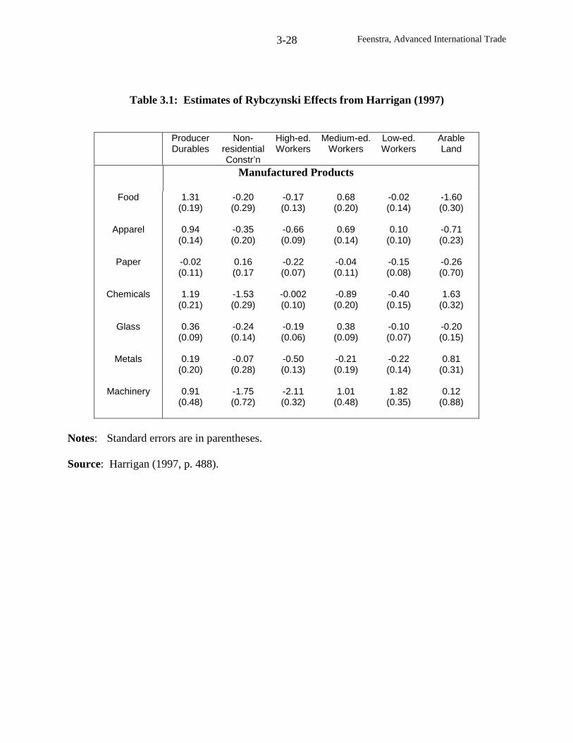
Feenstra, Advanced International Trade3-28
Table 3.1: Estimates of Rybczynski Effects from Harrigan (1997)
ProducerDurables
Non-residentialConstr’n
High-ed.Workers
Medium-ed.Workers
Low-ed.Workers
ArableLand
Manufactured Products
Food 1.31(0.19)
-0.20(0.29)
-0.17(0.13)
0.68(0.20)
-0.02(0.14)
-1.60(0.30)
Apparel 0.94(0.14)
-0.35(0.20)
-0.66(0.09)
0.69(0.14)
0.10(0.10)
-0.71(0.23)
Paper -0.02(0.11)
0.16(0.17
-0.22(0.07)
-0.04(0.11)
-0.15(0.08)
-0.26(0.70)
Chemicals 1.19(0.21)
-1.53(0.29)
-0.002(0.10)
-0.89(0.20)
-0.40(0.15)
1.63(0.32)
Glass 0.36(0.09)
-0.24(0.14)
-0.19(0.06)
0.38(0.09)
-0.10(0.07)
-0.20(0.15)
Metals 0.19(0.20)
-0.07(0.28)
-0.50(0.13)
-0.21(0.19)
-0.22(0.14)
0.81(0.31)
Machinery 0.91(0.48)
-1.75(0.72)
-2.11(0.32)
1.01(0.48)
1.82(0.35)
0.12(0.88)
Notes: Standard errors are in parentheses.
Source: Harrigan (1997, p. 488).
Feenstra, Advanced International Trade3-29
More Goods than Factors
We now consider a model with more goods than factors, and for convenience, suppose
that there are three goods and two factors (labor and capital). We assume that there is perfect
factor mobility between the industries. The zero profit conditions (3.1) then become 3 equations
in 2 unknowns, so we cannot find a solution except at special values of the prices (p1, p2, p3).
This situation is illustrated in Figure 3.6. If we consider one of these special prices (p1, p2, p3) at
which all 3 goods are produced, then the full-employment conditions (3.2) give 2 equations in 3
unknowns, so these are under-determined: there are many solutions for (y1, y2, y3). What is the
explanation for these unusual results?
Using the result that there are multiple solutions for (y1, y2, y3), we can graph these as a
line of outputs on the PPF in Figure 3.7. Therefore, the PPF has “ruled segments” on it, as
illustrated. Any price vector p=(p1, p2, p3) that allows for zero profits in all three industries will
correspond to a line of outputs along the PPF. At the same time, a slight movement in prices
away from this point will very likely lead to a corner solution, where only two of the goods are
produced. Thus, for most price vectors there will be specialization in a subset of goods, equal to
the number of factors. Conversely, if the price vector just happens to allow for zero-profits in all
goods, then there will be multiple solutions for the outputs.17
With these initial observations, what can we say about factor price equalization? At first
glance, the problem seems intractable: the set of goods produced in a country will be extremely
sensitive to the product prices. But let us recall that the prices being considered must be the
17 This means that the GDP function is not differentiable in the product prices.
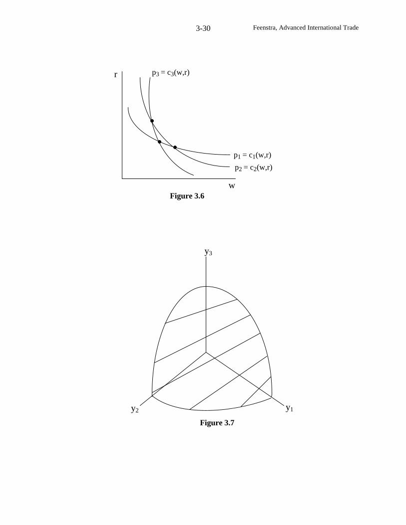
Feenstra, Advanced International Trade3-30
p1 = c1(w,r)
p2 = c2(w,r)
p3 = c3(w,r)
w
r
Figure 3.6
y3
y1y2
Figure 3.7
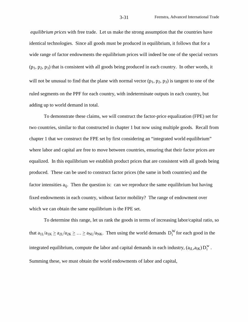
Feenstra, Advanced International Trade3-31
equilibrium prices with free trade. Let us make the strong assumption that the countries have
identical technologies. Since all goods must be produced in equilibrium, it follows that for a
wide range of factor endowments the equilibrium prices will indeed be one of the special vectors
(p1, p2, p3) that is consistent with all goods being produced in each country. In other words, it
will not be unusual to find that the plane with normal vector (p1, p2, p3) is tangent to one of the
ruled segments on the PPF for each country, with indeterminate outputs in each country, but
adding up to world demand in total.
To demonstrate these claims, we will construct the factor-price equalization (FPE) set for
two countries, similar to that constructed in chapter 1 but now using multiple goods. Recall from
chapter 1 that we construct the FPE set by first considering an “integrated world equilibrium”
where labor and capital are free to move between countries, ensuring that their factor prices are
equalized. In this equilibrium we establish product prices that are consistent with all goods being
produced. These can be used to construct factor prices (the same in both countries) and the
factor intensities aij. Then the question is: can we reproduce the same equilibrium but having
fixed endowments in each country, without factor mobility? The range of endowment over
which we can obtain the same equilibrium is the FPE set.
To determine this range, let us rank the goods in terms of increasing labor/capital ratio, so
that a1L/a1K > a2L/a2K > … > aNL/aNK. Then using the world demands WiD for each good in the
integrated equilibrium, compute the labor and capital demands in each industry, (aiL,aiK) wiD .
Summing these, we must obtain the world endowments of labor and capital,
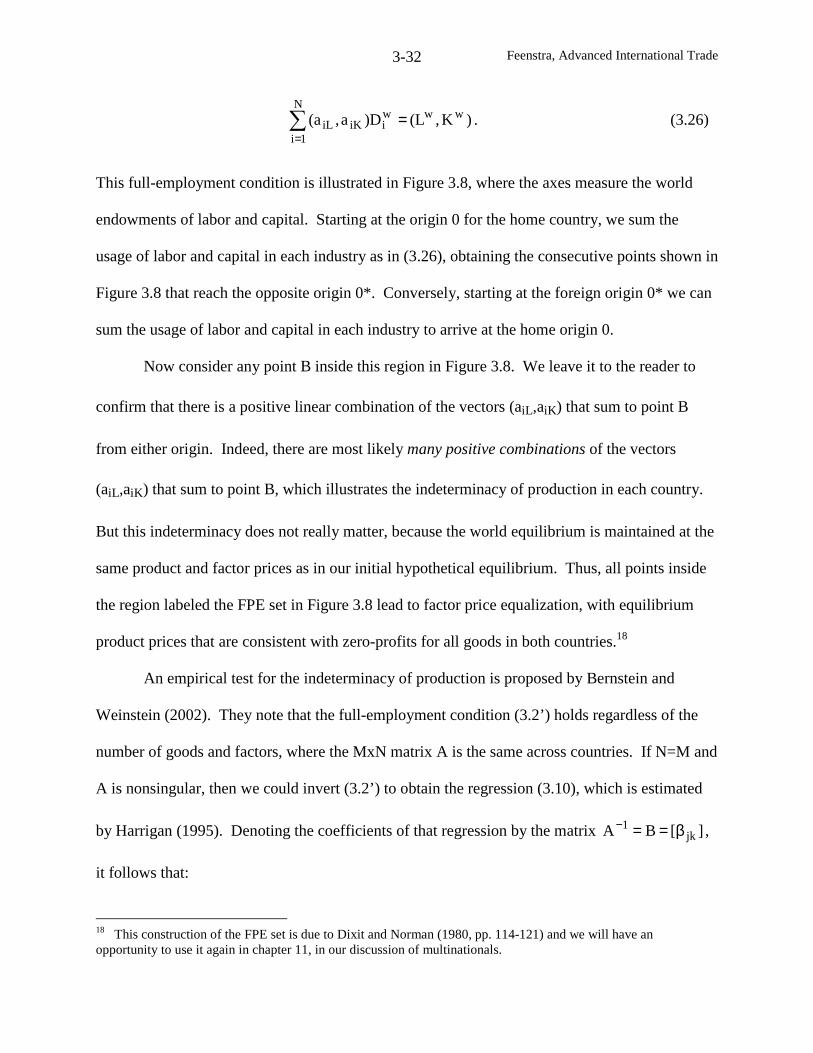
Feenstra, Advanced International Trade3-32
∑=
=N
1i
wwwiiKiL .)K,(L)Da,(a (3.26)
This full-employment condition is illustrated in Figure 3.8, where the axes measure the world
endowments of labor and capital. Starting at the origin 0 for the home country, we sum the
usage of labor and capital in each industry as in (3.26), obtaining the consecutive points shown in
Figure 3.8 that reach the opposite origin 0*. Conversely, starting at the foreign origin 0* we can
sum the usage of labor and capital in each industry to arrive at the home origin 0.
Now consider any point B inside this region in Figure 3.8. We leave it to the reader to
confirm that there is a positive linear combination of the vectors (aiL,aiK) that sum to point B
from either origin. Indeed, there are most likely many positive combinations of the vectors
(aiL,aiK) that sum to point B, which illustrates the indeterminacy of production in each country.
But this indeterminacy does not really matter, because the world equilibrium is maintained at the
same product and factor prices as in our initial hypothetical equilibrium. Thus, all points inside
the region labeled the FPE set in Figure 3.8 lead to factor price equalization, with equilibrium
product prices that are consistent with zero-profits for all goods in both countries.18
An empirical test for the indeterminacy of production is proposed by Bernstein and
Weinstein (2002). They note that the full-employment condition (3.2’) holds regardless of the
number of goods and factors, where the MxN matrix A is the same across countries. If N=M and
A is nonsingular, then we could invert (3.2’) to obtain the regression (3.10), which is estimated
by Harrigan (1995). Denoting the coefficients of that regression by the matrix ][BA jk1 β==− ,
it follows that:
18 This construction of the FPE set is due to Dixit and Norman (1980, pp. 114-121) and we will have anopportunity to use it again in chapter 11, in our discussion of multinationals.
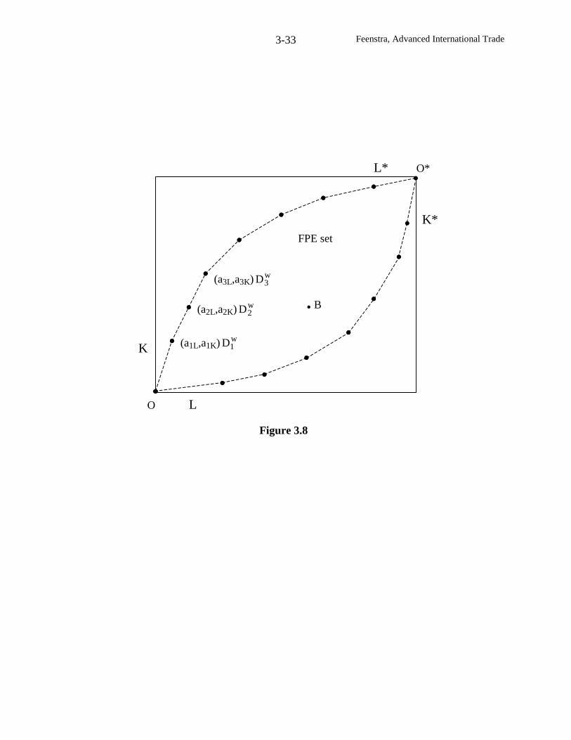
Feenstra, Advanced International Trade3-33
O L
K
K*
L* O*
Figure 3.8
(a1L,a1K) w1D
(a2L,a2K) w2D
(a3L,a3K) w3D
. B
FPE set
Feenstra, Advanced International Trade3-34
AB = IM, (3.27)
where IM is an identity matrix of dimension M. Thus, a test for the indeterminacy of production
proceeds by estimating the regression (3.10) as in Harrigan, and using the coefficients to test the
linear restriction in (3.27). If these fail, we conclude that production is indeterminate.
Bernstein and Weinstein use data across 47 Japanese prefectures around 1985, with 29
sectors and 3 factors (college-educated workers, other workers and capital). They first check
whether the full-employment condition AYi = Vi holds for each prefecture i=1,…,47. In this
test, the matrix A is held fixed at its national value for Japan. This means that the national full-
employment condition ∑∑ == = 471i
i471i
i VYA holds by construction, and the first test is to see
whether this condition also holds for each prefecture. This first test passes easily. However,
they strongly reject the second test, which consists of estimating regression (3.10) using the
cross-prefecture data and testing restriction (3.27). The implication is that the location of
production across the prefectures in Japan is not simply explained by the endowments in each
region: some other features must be at work.19
Is there any way to resolve production indeterminacy when there are more goods than
factors? Bhagwati (1972), responding to Jones (1956-57), suggested that a determinate
production structure would occur when factor prices were unequal across countries: in that case,
every commodity exported by a country with high labor/capital endowment would need to have a
higher labor/capital ratio than the exports of the other country. A proof of this so-called “chain
19 Other features are suggested by Davis and Weinstein (2001b), which is recommend for further reading.Bernstein and Weinstein (2002) go on to compare their results for Japan to those obtained with international data.
They find that even the full-employment condition AYi
= Vi
fails when using the Japanese national data for A but
this is not the case for when using other country’s data for Yi
and Vi. This is the familiar finding that production
techniques differ across countries.
Feenstra, Advanced International Trade3-35
proposition” was provided by Deardorff (1979). Bhagwati also suggested that the existence of
transportation costs would be enough to make factor prices unequal, and therefore resolve the
production indeterminacy. Deardorff argued that this is true when there is only trade in final
goods (and no subsidies to trade), but it breaks down when there is also trade in intermediate
inputs. Setting aside this concern, are there any other cases where production indeterminacy can
be resolved? Instead of relying on transportation costs to generate factor price differences, it
would seem that we could instead rely on endowment differences between the countries, large
enough to move them outside of the factor-price equalization set. This turns out to be a fruitful
line of inquiry, and to model it most elegantly, it will be useful to introduce a continuum of
products into the Heckscher-Ohlin model. This is done by Dornbusch, Fischer and Samuelson
(1980), which we discuss next.
Continuum of Goods
Let z∈ [0,1] denote the range of goods, and let y(z) denote the quantity produced of each
of these goods:
y(z) = z]K(z),[L(z),f , (3.28)
where these production functions are increasing, concave and linearly homogeneous in
[L(z),K(z)] . It will be convenient to work with the dual unit-cost functions, which are:
c(w,r,z) }1z]K(z),[L(z),f|rK(z)L(z)w{min0)z(K),z(L
≥+≡≥
. (3.29)
We let aL(w,r,z) ≡ ∂c(w,r,z)/∂w and aK(w,r,z) ≡ ∂c(w,r,z)/∂r denote the amount of labor and
capital, respectively, needed to produce one unit of y(z). These will depend on the factor prices,
Feenstra, Advanced International Trade3-36
but we assume that there are no factor-intensity reversals, which means that we can order the
activities z such that aK(w,r,z)/aL(w,r,z) is non-decreasing in z. That is, we rank the activities by
increasing order of capital-intensity.
Consider first the home country under autarky. Demand is assumed to come from a
Cobb-Douglas utility function:
∫∫ =αα= 1
0
1
01dz)z(with,dz)z(yln)z(Uln . (3.30)
Thus, a constant share of income α(z) is spent on each final good y(z). Under autarky, then, the
expenditure on each final good at home would be α(z)(wL+rK), where L and K are the factor
endowments, with equilibrium prices w and r. Dividing this by the prices p(z)=c(w,r,z), we
obtain demand for each output, which must equal supply under autarky:
y(z) = α(z)(wL+rK)/c(w,r,z). (3.31)
To complete the equilibrium conditions, we use the equality of factor demand and factor
supply, which is written in relative terms as:
∫
∫=
1
0 K
1
0 L
dz)z(y)z,r,w(a
dz)z(y)z,r,w(a
K
L. (3.32)
The numerator on the right of (3.32) is the total demand for labor, and the denominator is the
total demand for capital, which must equal their relative endowments. Substituting (3.31) into
Feenstra, Advanced International Trade3-37
(3.32), we obtain one equation to determine the factor price ratio (w/r) in autarky.20
Let us now introduce the foreign country, denoted with an asterisk, and having the
identical technology and tastes as at home. The key issue for trade is to determine which goods
are produced in each country. Under factor price equalization this will be impossible to
determine. In that case, the equilibrium prices are still p(z)=c(w,r,z), and condition (3.31) is
modified as:
y(z) + y*(z) = α(z)[(wL+rK)+ (wL*+rK*)]/c(w,r,z) , (3.31’)
where y(z) is the home outputs and y*(z) is foreign output. The only condition that ties down
these outputs is (3.32) in each country: the relative demand for labor must equal its relative
endowments. But there are many combinations of outputs y(z) and y*(z) that will
simultaneously satisfy (3.31’) and condition (3.32) in each country. Neither outputs nor the set
of goods produced in each country are uniquely determined, just as we found in the previous
section under factor price equalization.
If factor endowments are sufficiently different, however, then factor price (w*,r*) will
differ from (w,r). Notice that the FPE set can be constructed just as we did in the previous
section, and it is illustrated in Figure 3.9. Instead of the piece-wise linear segments obtained
from the full-employment condition (3.26), we instead have smooth curves in Figure 3.9
obtained by integrating over the factor demands [aL(w,r,z),aK(w,r,z)]Dw(z), where world demand
Dw(z) in the integrated equilibrium equals (3.31’). A point like B right on the boundary of the
FPE set, and would allow for factor-price equalization, but for endowments just slightly to the
20 Notice that demand on the right of (3.31) depends only on the factor price ratio, since c(w,r,z) is homogeneous of
degree one in (w,r). Similarly, aL(w,r,z) ≡ cw(w,r,z) and aK(w,r,z) ≡ cr(w,r,z) in (3.32) depend on the factor priceratio, since these factor demands are homogeneous of degree zero in (w,r).
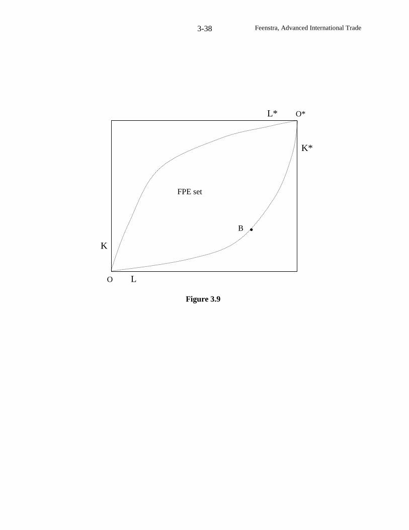
Feenstra, Advanced International Trade3-38
O L
K
K*
L* O*
Figure 3.9
FPE set
B .
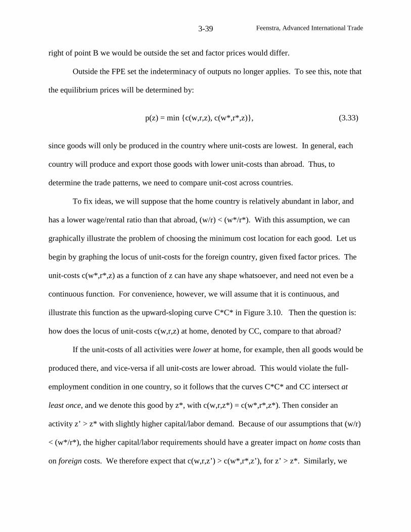
Feenstra, Advanced International Trade3-39
right of point B we would be outside the set and factor prices would differ.
Outside the FPE set the indeterminacy of outputs no longer applies. To see this, note that
the equilibrium prices will be determined by:
p(z) = min {c(w,r,z), c(w*,r*,z)}, (3.33)
since goods will only be produced in the country where unit-costs are lowest. In general, each
country will produce and export those goods with lower unit-costs than abroad. Thus, to
determine the trade patterns, we need to compare unit-cost across countries.
To fix ideas, we will suppose that the home country is relatively abundant in labor, and
has a lower wage/rental ratio than that abroad, (w/r) < (w*/r*). With this assumption, we can
graphically illustrate the problem of choosing the minimum cost location for each good. Let us
begin by graphing the locus of unit-costs for the foreign country, given fixed factor prices. The
unit-costs c(w*,r*,z) as a function of z can have any shape whatsoever, and need not even be a
continuous function. For convenience, however, we will assume that it is continuous, and
illustrate this function as the upward-sloping curve C*C* in Figure 3.10. Then the question is:
how does the locus of unit-costs c(w,r,z) at home, denoted by CC, compare to that abroad?
If the unit-costs of all activities were lower at home, for example, then all goods would be
produced there, and vice-versa if all unit-costs are lower abroad. This would violate the full-
employment condition in one country, so it follows that the curves C*C* and CC intersect at
least once, and we denote this good by z*, with c(w,r,z*) = c(w*,r*,z*). Then consider an
activity z’ > z* with slightly higher capital/labor demand. Because of our assumptions that (w/r)
< (w*/r*), the higher capital/labor requirements should have a greater impact on home costs than
on foreign costs. We therefore expect that c(w,r,z’) > c(w*,r*,z’), for z’ > z*. Similarly, we
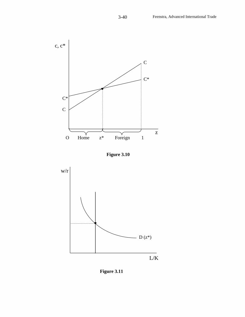
Feenstra, Advanced International Trade3-40
D (z*)
L/K
w/r
Figure 3.11
z
C
C*
C*
C
O Home z* Foreign 1
Figure 3.10
c, c*
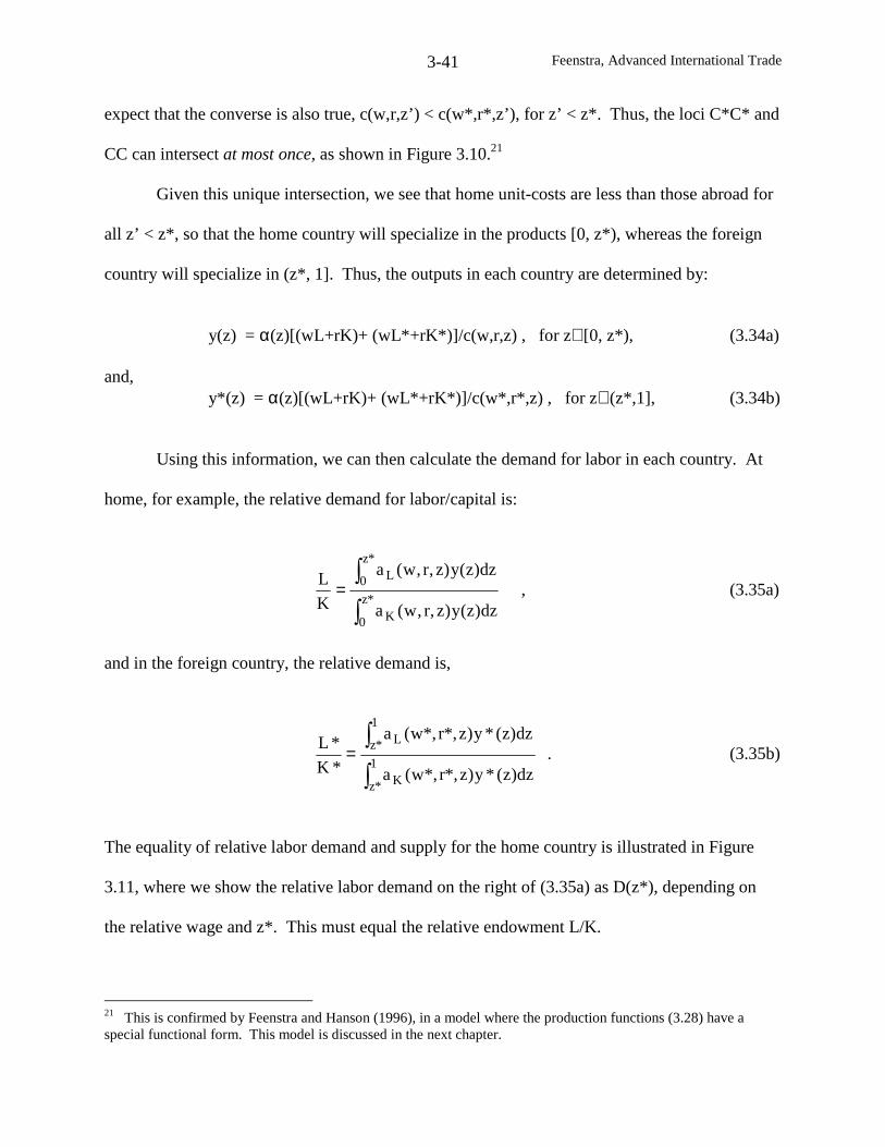
Feenstra, Advanced International Trade3-41
expect that the converse is also true, c(w,r,z’) < c(w*,r*,z’), for z’ < z*. Thus, the loci C*C* and
CC can intersect at most once, as shown in Figure 3.10.21
Given this unique intersection, we see that home unit-costs are less than those abroad for
all z’ < z*, so that the home country will specialize in the products [0, z*), whereas the foreign
country will specialize in (z*, 1]. Thus, the outputs in each country are determined by:
y(z) = α(z)[(wL+rK)+ (wL*+rK*)]/c(w,r,z) , for z∈ [0, z*), (3.34a)
and,y*(z) = α(z)[(wL+rK)+ (wL*+rK*)]/c(w*,r*,z) , for z∈ (z*,1], (3.34b)
Using this information, we can then calculate the demand for labor in each country. At
home, for example, the relative demand for labor/capital is:
∫
∫=
*z
0 K
*z
0 L
dz)z(y)z,r,w(a
dz)z(y)z,r,w(a
K
L, (3.35a)
and in the foreign country, the relative demand is,
∫
∫=
1
*z K
1
*z L
dz)z(*y)z*,r*,w(a
dz)z(*y)z*,r*,w(a
*K
*L. (3.35b)
The equality of relative labor demand and supply for the home country is illustrated in Figure
3.11, where we show the relative labor demand on the right of (3.35a) as D(z*), depending on
the relative wage and z*. This must equal the relative endowment L/K.
21 This is confirmed by Feenstra and Hanson (1996), in a model where the production functions (3.28) have aspecial functional form. This model is discussed in the next chapter.
Feenstra, Advanced International Trade3-42
The two-country equilibrium is determined by conditions (3.34) and (3.35), combined
with c(w,r,z*) = c(w*,r*,z*), and also trade balance between the countries:
∫ ∫ +α=+α1
*z
*z
0dz)K*rL*w)(z(dz)rKwL)(z( (3.36)
The left of (3.36) is the value of home imports of the goods (z*, 1], while the right-side is home
exports of those products [0, z*). Substituting (3.34) into (3.35), we have four equations [i.e.
(3.35a), (3.35b), c(w,r,z*) = c(w*,r*,z*) and (3.36)] to determine z* and the four factor prices
(w,r), and (w*,r*), where one factor price can be normalized at unity.
Summing up, when factor price are not equalized across the countries, we have shown
that each country is specialized in a different range of final goods. Not only have we resolved
the indeterminacy of outputs, we have gone much further: there is an extremely strong
connection between the labor/capital ratios in production and the labor/capital endowments, with
all the goods [0, z*) produced by the labor-abundant country having a higher labor/capital ratio
in production than all the goods (z*, 1] produced by the capital-abundant country. This holds
even for slight differences in the factor prices across countries, i.e., for factor endowments just
slightly to the right of point B in Figure 3.9.
Estimating the HOV Model Once Again
We return now to the estimation of the Heckscher-Ohlin-Vanek (HOV) model, and the
recent results of Davis and Weinstein (2001a). Recall that the key issue in estimating the HOV
model is to allow for some technological differences across countries, while avoiding the
introduction of so many free parameters that the HOV equation holds as an equality (as in
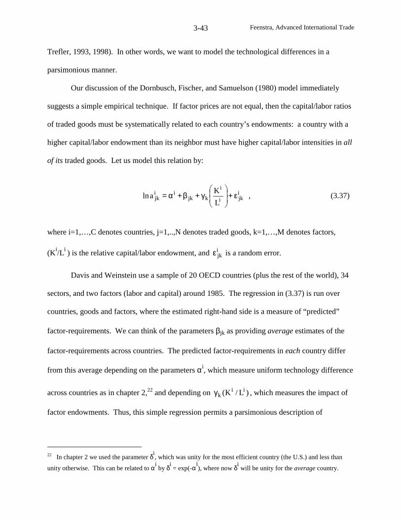
Feenstra, Advanced International Trade3-43
Trefler, 1993, 1998). In other words, we want to model the technological differences in a
parsimonious manner.
Our discussion of the Dornbusch, Fischer, and Samuelson (1980) model immediately
suggests a simple empirical technique. If factor prices are not equal, then the capital/labor ratios
of traded goods must be systematically related to each country’s endowments: a country with a
higher capital/labor endowment than its neighbor must have higher capital/labor intensities in all
of its traded goods. Let us model this relation by:
ijki
i
kjkii
jkL
Kaln ε+
γ+β+α= , (3.37)
where i=1,…,C denotes countries, j=1,..,N denotes traded goods, k=1,…,M denotes factors,
(Ki/Li ) is the relative capital/labor endowment, and ijkε is a random error.
Davis and Weinstein use a sample of 20 OECD countries (plus the rest of the world), 34
sectors, and two factors (labor and capital) around 1985. The regression in (3.37) is run over
countries, goods and factors, where the estimated right-hand side is a measure of “predicted”
factor-requirements. We can think of the parameters βjk as providing average estimates of the
factor-requirements across countries. The predicted factor-requirements in each country differ
from this average depending on the parameters αi, which measure uniform technology difference
across countries as in chapter 2,22 and depending on )L/K( iikγ , which measures the impact of
factor endowments. Thus, this simple regression permits a parsimonious description of
22 In chapter 2 we used the parameter δi, which was unity for the most efficient country (the U.S.) and less than
unity otherwise. This can be related to αiby δi
= exp(-αi), where now δi
will be unity for the average country.
Feenstra, Advanced International Trade3-44
technology differences across countries.
As noted by Harrigan (2003), there is considerable prior evidence that a specification like
(3.37) will fit the data quite well: Dollar, Wolff and Baumol (1988, Table 2.3), for example, find
that capital per worker in individual industries is highly correlated with capital per worker in
overall manufacturing. Davis and Weinstein (2001a) likewise find that the simple linear
relationship (3.37) fits well, and that the parameters γk linking factor-requirements to country
endowments are highly significant. Using several variants of this regression, they construct the
estimated technology matrix iA for each country using the predictions from (3.37). This
estimated matrix is then used to construct the factor content of trade, and evaluate how well the
constructed factor contents match the relative endowments of countries. In other words, we can
proceed much as in the earlier testing of the HOV model, but now using technology matrices
iA ,which differ across countries.
As discussed near the end of the last chapter, when the technology matrices differ across
countries, then we should use the technology of the exporting country to construct the factor
content of trade. Davis and Weinstein follow this approach, so the factor content of exports from
country i to country j is:
ijiij XAF ≡ , (3.38)
where Xij is the vector of gross exports of goods from country i to j. Davis and Weinstein
sometimes use an additional assumption, whereby these exports are themselves estimated in
proportion to the purchasing country’s GDP. In that case, the factor content of export is:
ijiij XAF ≡ . (3.39)
Feenstra, Advanced International Trade3-45
In either case, the prediction of the HOV model is that the factor content of trade reflects a
country’s relative endowments, or that:
Vi– s
i(∑ j
jV ) = (∑ ≠ijijF ) – (∑ ≠ij
jiF ). (3.40)
In the sign test, for example, if we assume that all OECD countries use the same average
technology matrix, then we include only the parameters βjk in regression (3.37) and construct the
predicted technology matrix A , which is the same across countries. In that case, Davis and
Weinstein initially find that the right and left-sides of (3.40) have the same sign in only 46% of
the cases.23 This is no better than a coin toss, much as we found in chapter 2. If instead we
allow for uniform productivity differences δi between countries, so the regression (3.37) is
estimated with αiin addition to βjk, then we find that the sign test is satisfied in 50% of the
cases. If we also include )L/K( iikγ in regression (3.37), so that the estimated technologies
differ systematically with countries’ factor endowments, then the sign test is satisfied in fully
86% of the cases. Finally, if we model exports as proportional to the purchasing countries GDP,
so factor contents are measured with (3.39) rather than (3.38), than the sign test is satisfied in
92% of the cases!
Clearly, we are getting closer to a 100% match between relative endowments and
constructed factor contents, on the left and right of (3.40). The theorem of Trefler (1998)
reviewed in the previous chapter tells us that this is no coincidence: if regression (3.37) fit
perfectly, and using the assumption that every good is exported in proportion to the purchasing
country’s GDP, then (3.40) would automatically hold. What is remarkable is that even the
23 We average the results reported for labor and capital in Davis and Weinstein (2001a, Table 4).
Feenstra, Advanced International Trade3-46
simple specification in (3.37) is enough to greatly improve the fit of the HOV model. The
contribution of Davis and Weinstein is to systematically show the importance of each modeling
assumption to “closing the gap” between factor contents and endowments.
Conclusions
We have covered a lot of ground in this chapter. As we leave the “even” structure of the
2x2 or the NxN model, many of the results we found in chapter 1 are lost. With more factors
than goods, the “factor price insensitivity” lemma no longer applies. This can be tested by
estimating a GDP function for a country (or a group of countries), and determining whether it is
linear in the factor endowments, i.e. whether the functional form in (3.7) holds globally or the
elasticities in (3.22) are locally insignificantly different from zero. The results of Kohli (1990,
1993a) for the U.S. indicate that the elasticities in (3.22) are non-zero, but only weakly so. This
can be interpreted as evidence in favor of “more factors than goods.” One reason for this is that
capital might be slow to move between sectors, so with N sectors there are N fixed factors
(capital in each sector) plus the additional mobile factors (types of labor). Kohli (1993b)
develops a test for this production structure and finds some evidence to support it using annual
data for the U.S..
With more factors than goods, the GDP function is generally well behaved: it will be
differentiable in prices and endowments provided that industries do not have the same factor
intensities. With more goods than factor, however, the GDP function is poorly behaved: the fact
that the production possibility frontier has “ruled segments,” as illustrated in Figure 3.7, indicates
that the GDP function is not differentiable in prices. A test for “more goods than factors” is
developed by Bernstein and Weinstein (2002), and they find evidence to support this using data
from prefectures in Japan. This may seem inconsistent with the results of Kohli (1993b) for the
Feenstra, Advanced International Trade3-47
U.S., but note that Kohli used time-series data whereas Bernstein and Weinstein used cross-
sectional data. We should not be surprised to find differing conclusions when comparing the
time-series of national data versus the cross-section of provincial data. In any case, the results of
both Kohli and Bernstein and Weinstein support the idea that we are not in an “even” model,
with equal numbers of goods and factors. This structure had been assumed by Leamer (1984)
and Harrigan (1995), for example. The more general approach of Harrigan (1997), using a GDP
function estimated across OECD countries, could also be used to test “factor price insensitivity”
by evaluating the elasticities in (3.22), though this was not done due to data limitations.
We have also reviewed the Heckscher-Ohlin model with a continuum of goods, due to
Dornbusch, Fischer and Samuelson (1980). This was used to motivate the empirical work of
Davis and Weinstein (2001a). Using the idea that industry factor intensities should depend
systematically on economy-wide factor endowments, Davis and Weinstein estimate technology
matrices across the OECD countries and use these to test the HOV equation. We already know
from the theorem of Trefler (1998), discussed at the end of the last chapter, that using actual
technology matrices (and an assumption on exports) can lead to a perfect fit for this equation.
What is surprising is that Davis and Weinstein are able to obtain a very close fit even with a
parsimonious specification of the technology matrices across countries. In case the reader thinks
that this is the last word on the HOV model, however, we note that there are still important issues
left unresolved by Davis and Weinstein (2001a).
First, their sample consists of the OECD countries, and in any evaluation of the
Heckscher-Ohlin model we ideally want to introduce data on a wider range of countries. Xu
(2002) has recently estimated a regression like (3.37) over a sample of 14 developing countries.
By systematically examining the sign of the regression coefficient γk (which indicates the impact
Feenstra, Advanced International Trade3-48
of the countries’ capital/labor endowments on their industry capital/labor ratios), he is able to
arrange countries into three distinct groups, ranked by their capital/labor abundance. His
evidence supports the idea that these countries are in different cones of diversification.
Second, Trefler and Zhu (2000) have criticized Davis and Weinstein’s approach for not
adequately distinguishing between trade in final goods and trade in intermediate inputs. All of
the theory we have developed for the HOV equation assumes trade in final goods, and yet, a
great deal of actual trade is in steel, chemicals, textiles, and other intermediate inputs. Indeed,
component parts can cross borders multiple times before being incorporated into a finished good.
This makes the construction of the factor content of trade very difficult: if Germany imports
steel from Korea, and Korea relied on coal from Australia to produce the steel, and Australia
used imported mining equipment from Germany, then whose factor requirements should we use
to construct the factor content of steel trade? These types of flows tend to cancel out when we
consider only net exports of each country, as in the original formulation of the HOV model.
However, once the technology matrices differ across countries, then totaling up the gross exports
as on the right of (3.40) can lead to considerably larger values for trade, much of which is due to
intermediate inputs. It is hard to see, then, how achieving near-equality of (3.40) amounts to a
validation of the HOV model, when that model has so little to say about trade in intermediate
inputs. Trefler (1998) and Davis and Weinstein (2003) concur that this is an important area for
further research, and one that we begin to investigate in the next chapter.
3-49
Problems
3.1 In the sector-specific model, suppose that the home and foreign countries have identical labor
and capital in sector 2, but the home country has more capital in sector 1. Technologies and
tastes are the same across countries.
(a) Can we predict the trade pattern between the countries? What factor(s) at home benefit from
the opening of trade, and which factor(s) lose?
(b) Repeat part (a), but now assume that the endowments of capital are identical across the
countries, but the home country has more labor. Can we predict the trade pattern between the
countries? Try to use assumptions on the factor cost shares to help determine this.
3.2 Consider the translog GDP function )V,p(Gln in (3.15).
(a) Show that G(p,V) is homogeneous of degree one in prices when (3.16) and γij = γji hold.
(b) Show that G(p,V) is homogeneous of degree one in endowments when (3.17) and lkδ = klδ
hold.
3.3 Suppose that there are two outputs – nontraded good 1 and traded good 2 – and three inputs –
labor, capital, and imported inputs. Assume that the cost share of labor is higher in good 1 and
the cost share of capital is higher in good 2. The prices of both outputs are treated as fixed
initially, but the price of the imported input increases.
(a) Write down the zero-profit conditions and totally differentiate these.
(b) Determine the impact of the increase in the imported input price on the wage and rental,
assuming that the traded good has a higher cost share of imports.
(c) If the price of the nontraded good changes endogenously due to the increase in the price of
imported inputs, how will this affect your conclusions in (b)?
Feenstra, Advanced International Trade
Chapter 4: Trade in Intermediate Inputs and Wages
Since the early 1980s there has been a marked change in the pattern of wage payments in
the United States: the wage of skilled relative to unskilled workers experienced a sustained
increase, that continued through the 1990s. A similar pattern was observed in other countries.
This led to a great deal of research on the possible causes of the change in relative wages.1 From
the material we have already covered, we can identify three methods to determine whether the
change in relative wages is due to international trade.
First, we could estimate a GDP or cost function for the U.S. economy, or for specific
industries, and compute the Stolper-Samuelson effect of a change in traded goods prices. We
will discuss this approach at several points throughout the chapter. Second, we could proceed as
in the Heckscher-Ohlin-Vanek (HOV) model and compute the change in the factor content of
trade and associated changes in factor prices. Theoretically, this second approach is justified by
Deardorff and Staiger (1988), who show that:
,0)FF)(ww( 1212 ≥−− (4.1)
where wi are equilibrium wages in a country in two equilibria i=1,2, and Fi is the factor-content
of exports for that country. Equation (4.1) is interpreted as saying that a higher content of
imports for some factor k, 0FF 1k
2k << so 0)FF( 1
k2k <− , will tend to be associated with a falling
wage for that factor, 0)ww( 1k
2k <− . The same would be true for the direct import of a factor,
as with immigration. Among the most careful assessment of these effects for the United States,
1 See the surveys by Feenstra (1998), Freeman (1995), Johnson and Stafford (1999), Katz and Autor (1999),Richardson (1995) and Wood (1995), and the volumes by Bhagwati and Kosters (1994), Cheng and Kierzkowski(2001), Collins (1998) and Feenstra (2000). This chapter draws upon Feenstra and Hanson (2003).
Feenstra, Advanced International Trade4-2
Borjas, Freeman and Katz (1997, p. 62) find that immigration into the U.S. during 1980-1995
accounts for about one-quarter to one-half of the decline in the relative wages of high-school
dropouts. The increasing factor content of imports from less-developed countries also has some
effect on reducing the wages of high-school dropouts, but by less than immigration. Both
channels have only a small impact on the wages of more highly-educated workers.
Note the similarity between (4.1), which refers to a comparison over time, and equation
(2.19) (from Helpman, 1984a), which referred to a comparison across countries. This suggests
that all the observations we have made about testing the HOV model apply equally well to
implementing formula (4.1): the results of a factor-content approach when applied over time
will depend on the assumptions about technology (which year or country’s technology matrix is
used); assumptions on tastes; and also whether or not there are traded intermediate inputs.2 For
these reasons, there is considerable controversy about the suitability of using a factor-content
approach to infer the effects of trade on wages.3
These concerns suggest a third approach: rather than relying on an HOV equation, let us
directly model the presence of traded intermediate inputs, caused by firms splitting apart their
production process across several countries. This is sometimes called “production sharing” by
the companies involved, or simply “outsourcing.”4 The idea that trade in intermediate inputs
can have an effect on production and factor prices that is different from trade in final goods is
2 Note that Staiger (1986) argues that traded intermediate inputs should not be included in the calculation of factor-contents in the bilateral test of Helpman (1984a), so their treatment in applying the factor-content approach overtime is open to question.3 See Deardorff (2000), Krugman (2000), Leamer (2000), and Panagariya (2000).4 Alternatively referred to as outsourcing (Katz and Murphy, 1992, Feenstra and Hanson, 1996), de-localization(Leamer, 1996), fragmentation (Jones and Keirzkowski, 1997, Arndt and Kierzkowski, 2000, Marjit and Acharyya,forthcoming), intra-product specialization (Arndt, 1997 and 1998a,b), intra-mediate trade (Antweiler and Trefler,2002), vertical specialization (Hummels, Ishii, and Yi, 2001), and slicing the value chain (Krugman, 1995), thisphenomena refers to the geographic separation of activities involved in producing a good (or service) across two ormore countries. The term “production sharing” was coined by management consultant Peter Drucker (“The Rise ofProduction Sharing,” The Wall Street Journal, March 15, 1977).
Feenstra, Advanced International Trade4-3
gaining widespread acceptance among trade economists,5 and no graduate trade course today is
complete without a discussion of this topic (I think the same is true at the undergraduate level).
Fortunately, the tools we have developed in the previous chapters can be readily extended to deal
with trade in intermediate inputs.
After reviewing the initial evidence concerning the change in wages for the U.S. in the
next section, we present a simple three-good, three-factor model that can be used to analyze the
link between input prices and wages. Two of the goods are traded intermediate inputs, and the
third is a final product. It is readily shown that a fall in the price of imported intermediate inputs
decreases the relative wage of the factor used intensively in those imports, which would be
unskilled labor for the U.S. Next, we generalize this model and present a version with a
continuum of inputs, analogous to the Dornbusch, Fischer, and Samuelson (1980) model. With
the U.S. being more abundant in skilled labor than abroad, the model predicts that a growth in
capital or technology abroad will lead to increased outsourcing from the U.S., and an increase in
the relative wage of skilled labor in both countries. Following this we discuss various methods
of estimating the model, and summarize evidence for the U.S. and other countries.
Changes in Wages and Employment
The basic facts concerning wage movements in the United States are well understood.6
For full-time U.S. workers between 1979 and 1995, the real wages of those with 12 years of
education fell by 13.4% and the real wages of those with less than 12 years of education fell by
20.2%. During the same period, the real wages of workers with 16 or more years of education
rose by 3.4%, so that the wage gap between less-skilled and more-skilled workers increased
5 In addition to the references in the previous footnote, see the Ohlin lectures of Jones (2000) and the recent articleby Paul Samuelson (2001).6 For a detailed discussion, see Katz and Autor (1999) whose wage figures we report below.
Feenstra, Advanced International Trade4-4
dramatically.7 To illustrate these trends, we can use data from the U.S. manufacturing sector for
“nonproduction” and “production” workers. The former are often used as a proxy for more-
skilled workers, and the latter as a proxy for less-skilled workers. The breakdown is far from
perfect, of course, but has been used because the data are readily available.8 These trends are
shown in Figure 4.1, which graphs the relative annual earnings of nonproduction/production
workers in U.S. manufacturing, and Figure 4.2, which illustrates their relative annual
employment.
In Figure 4.1, we see that earnings of nonproduction relative to production workers in the
U.S. moved erratically during the 1960s and 1970s, but then increased substantially during the
1980s and 1990s. Turning to Figure 4.2, we see that there has been a steady increase in the ratio
of nonproduction to production workers used in U.S. manufacturing, with some leveling off
recently. This increase in the supply of workers can account for the reduction in the relative
wage of nonproduction workers from 1970 to the early 1980s, as shown in Figure 4.1, but is at
odds with the increase in the relative nonproduction wage after that. The rising relative wage
should have led to a shift in employment away from skilled workers, along a demand curve, but
it has not. Thus, the only explanation consistent with these facts is that there has been an
outward shift in the demand for more-skilled workers since the mid-1980s, leading to an increase
in their relative employment and wages.9
7 Only the highly skilled have had large real-wage gains. For the 1979-1995 period, real wages for those with 18 ormore years of education rose by 14.0% and for those with 16 to 17 years of education rose by only 1.0%.8 The breakdown of workers according to whether or not they are engaged in production activity is made in the U.S.Annual Survey of Manufactures, and is used as a proxy for the occupational-class or skill-level of workers. Inpractice, this classification shows similar trends as using education or other skill categories (Berman, Bound andGriliches, 1994; Sachs and Schatz, 1994). The increase in the nonproduction/production relative wage is only asmall part of the total increase in wage inequality, however (Katz and Autor, 1999).9 The same decline in the relative wages of blue-collar workers during the 1980’s and into the 1990’s can be foundfor Australia, Canada, Japan, Sweden, and the United Kingdom (Freeman and Katz, 1994; Katz and Autor, 1999),and also for Hong Kong and Mexico (Cragg and Epelbaum, 1996; Hanson and Harrison, 1999; Hsieh and Woo,1999; Robertson, 2000).
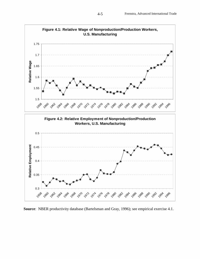
Feenstra, Advanced International Trade4-5
Figure 4.1: Relative Wage of Nonproduction/Production Workers,U.S. Manufacturing
1.5
1.55
1.6
1.65
1.7
1.75
1958
1960
1962
1964
1966
1968
1970
1972
1974
1976
1978
1980
1982
1984
1986
1988
1990
1992
1994
1996
Rel
ativ
eW
age
Figure 4.2: Relative Employment of Nonproduction/ProductionWorkers, U.S. Manufacturing
0.3
0.35
0.4
0.45
0.5
1958
1960
1962
1964
1966
1968
1970
1972
1974
1976
1978
1980
1982
1984
1986
1988
1990
1992
1994
1996
Rel
ativ
eE
mp
loym
ent
Source: NBER productivity database (Bartelsman and Gray, 1996); see empirical exercise 4.1.

Feenstra, Advanced International Trade4-6
What factors could lead to an outward shift in the relative demand for skilled labor in the
economy? One explanation suggested by the two-sector model is that the output of skill-
intensive sectors have risen relative to those of unskilled-labor intensive sectors: this would
certainly increase the relative demand for skilled labor. However, the evidence for the U.S. is
that this sort of sectoral change in outputs did not occur. Rather, the bulk of the increase in the
relative demand for skilled labor occurred within the manufacturing industries, and not by shifts
in labor between industries. Some evidence on this within versus between industry distinction is
contained in Table 4.1, which is taken from Berman, Bound and Griliches (1994).
Table 4.1 decomposes the change in the relative employment and relative wages of
nonproduction workers into those that occurred within and between industries. We can see that
in the period 1979-1987, the relative employment of nonproduction workers increased by
slightly more than one-half of one percent per year (0.55%), with about two-thirds of that
(0.36%) explained by within industry movements. On the wage side, the relative annual earnings
of nonproduction workers increased by about seven-tenths of a percentage point per year
(0.72%), with more than half of that change (0.41%) explained by within industry movements.
The conclusion suggested by Berman, Bound and Griliches (1994) is that trade cannot be a
dominant explanation for the wage and employment shifts, because the between industries
movements are smaller than the within industry movements.
This conclusion was reinforced by consideration of the price movements. If the Stolper-
Samuelson Theorem holds, then the relative price of skilled labor in the U.S. would increase if
the relative price of skill-intensive goods also increased, e.g. the price of computers rose relative
to the price of apparel. In fact, this did not occur during the 1980s.10 This can be seen from
10 But it did occur during the 1970s, in what Leamer (1998) has called the “Stolper-Samuelson decade.”
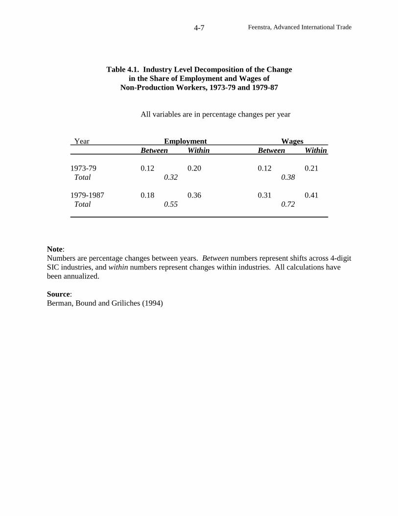
Feenstra, Advanced International Trade4-7
Table 4.1. Industry Level Decomposition of the Changein the Share of Employment and Wages of
Non-Production Workers, 1973-79 and 1979-87
All variables are in percentage changes per year
Year Employment WagesBetween Within Between Within
1973-79 0.12 0.20 0.12 0.21Total 0.32 0.38
1979-1987 0.18 0.36 0.31 0.41Total 0.55 0.72
Note:Numbers are percentage changes between years. Between numbers represent shifts across 4-digitSIC industries, and within numbers represent changes within industries. All calculations havebeen annualized.
Source:Berman, Bound and Griliches (1994)

Feenstra, Advanced International Trade4-8
Table 4.2, which is taken from the work of Lawrence and Slaughter (1993) and Lawrence
(1994). For each country, the first row is a weighted average of the change in manufacturing
prices over the 1980s, where the weights are the industry’s share of total manufacturing
employment of nonproduction workers. The second row is again the weighted average of the
change in prices over the 1980s, but now using the industry’s share of employment of production
workers. For U.S. import prices, for example, we can see that when industries are weighted by
their production workers, the average price increase is higher than when they are weighted by
non-production workers. The same pattern can be seen by comparing the rows for other
industrial countries. This means that some of the industries that use the most production – or
less-skilled – workers are those with the highest price increases. This finding led Lawrence and
Slaughter (1993) to conclude that the price movements, due to international competition, could
not explain the wage movements.
The price movements shown in Table 4.2, combined with the shift in relative demand
towards skilled labor within industries as shown in Table 4.1, led many economists to conclude
that international trade could not be a substantial explanation for the rise in relative wages.
Instead, they have looked to the introduction of skill-biased technological changes, such the
introduction of computers, to provide the explanation. But should we really rule out trade? It
may be true that the Heckscher-Ohlin model does not provide the explanation for the change in
wages during the 1980s and 1990s. But surely trade can have an important impact on the
structure of production, and demand for labor, within industries as well. This is certainly the
case when we introduce trade in intermediate inputs: as we shall see, trade can then affect labor
demand within an industry.
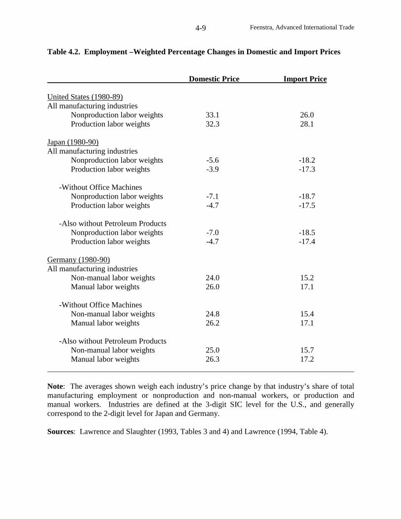
Feenstra, Advanced International Trade4-9
Table 4.2. Employment –Weighted Percentage Changes in Domestic and Import Prices
Domestic Price Import Price
United States (1980-89)All manufacturing industries
Nonproduction labor weights 33.1 26.0Production labor weights 32.3 28.1
Japan (1980-90)All manufacturing industries
Nonproduction labor weights -5.6 -18.2Production labor weights -3.9 -17.3
-Without Office MachinesNonproduction labor weights -7.1 -18.7Production labor weights -4.7 -17.5
-Also without Petroleum ProductsNonproduction labor weights -7.0 -18.5Production labor weights -4.7 -17.4
Germany (1980-90)All manufacturing industries
Non-manual labor weights 24.0 15.2Manual labor weights 26.0 17.1
-Without Office MachinesNon-manual labor weights 24.8 15.4Manual labor weights 26.2 17.1
-Also without Petroleum ProductsNon-manual labor weights 25.0 15.7Manual labor weights 26.3 17.2
Note: The averages shown weigh each industry’s price change by that industry’s share of totalmanufacturing employment or nonproduction and non-manual workers, or production andmanual workers. Industries are defined at the 3-digit SIC level for the U.S., and generallycorrespond to the 2-digit level for Japan and Germany.
Sources: Lawrence and Slaughter (1993, Tables 3 and 4) and Lawrence (1994, Table 4).
Feenstra, Advanced International Trade4-10
Some preliminary evidence which suggests that trade shifts the composition of activity
within an industry is provided by Bernard and Jensen (1997), who do the same decomposition as
Berman, Bound and Griliches but with plant-level data rather than industry-level data. This is
shown in Table 4.3. Looking again at the period 1979-1987, we can see that nearly one-half of
the relative increase in the employment of non-production workers (0.39%) occurred as a result
of the shifts between plants (0.18%), and more than one-half of the increase in the relative wage
of non-production workers (0.54%) is also explained by movements between manufacturing
plants (0.32%). Furthermore, Bernard and Jensen found that the plants experiencing the greatest
increase in relative nonproduction employment and earnings are precisely those that were
engaged in exporting.
The results of Bernard and Jensen provide prima facie evidence that trade has had an
impact on factor demand and wages, through shifting the demand for labor within industries. In
order to understand how these shifts due to trade can occur, we present in the next section a
simple model of outsourcing.
Trade in Intermediate Inputs: A Simple Model
Of the many activities that take place within any industry, let us identify just three: the
production of an unskilled-labor intensive input, denoted by y1 ; the production of a skilled-labor
intensive input, denoted by y2, and the “bundling together” of these two goods into a finished
product. The two intermediate inputs are produced at home and also traded internationally. We
shall simplify the analysis, however, by assuming that the production of these two inputs and the
“bundling” activity are always performed at home. Thus, we are ruling out “corner solutions”
where one of these activities is done entirely abroad. In reality, corner solutions such as this are
very common: e.g., many U.S. firms export intermediate inputs to the maquiladora plants in
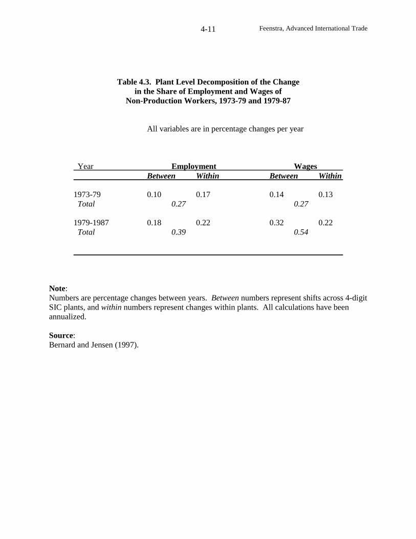
Feenstra, Advanced International Trade4-11
Table 4.3. Plant Level Decomposition of the Changein the Share of Employment and Wages of
Non-Production Workers, 1973-79 and 1979-87
All variables are in percentage changes per year
Year Employment WagesBetween Within Between Within
1973-79 0.10 0.17 0.14 0.13Total 0.27 0.27
1979-1987 0.18 0.22 0.32 0.22Total 0.39 0.54
Note:Numbers are percentage changes between years. Between numbers represent shifts across 4-digitSIC plants, and within numbers represent changes within plants. All calculations have beenannualized.
Source:Bernard and Jensen (1997).
Feenstra, Advanced International Trade4-12
Mexico, where assembly of the inputs and other production activities take place rather than in the
U.S.. A model that emphasizes the movement of entire activities across countries is presented in
the next section.
We will suppose that the two inputs yi, i=1,2, are each produced using unskilled labor
(Li), skilled labor (Hi), and capital (Ki), with concave and linearly homogeneous production
functions,
yi = fi(Li, Hi, Ki), i=1,2. (4.2)
For example, the unskilled-labor intensive input y1 might represent the activities done within a
factory, while the skilled-labor intensive input y2 might represent the research and development
activities within the industry, as well as marketing and after-sales service. These are both needed
to produce the final manufacturing product. But some of the activities done within the factory
can instead be outsourced, i.e. imported from abroad; and conversely, the services associated
with research, development and marketing can be exported to support production activities
abroad. We therefore let x1 < 0 denote the imports of input 1, and x2 > 0 denote the exports of
input 2. Also let pi denote the price of each input, i=1,2, and let p=(p1,p2) denote the price vector
of the traded intermediate inputs.
The production of the final good is given by yn = fn(y1-x1, y2-x2), where this production
function “bundles together” the amounts of goods 1 and 2 available, and is also concave and
linearly homogeneous. We ignore any additional labor and capital inputs used in this bundling
activity, so that the total factor usage in the manufacturing industry is,
L1+L2 = Ln, H1+H2 = Hn, K1+K2 = Kn . (4.3)
Feenstra, Advanced International Trade4-13
We can now solve for the optimal output in the industry, which includes the three
activities. With perfect competition, the value of output from the final good, plus net trade, will
be maximized subject to the resource constraints:
Gn(Ln, Hn, Kn, pn, p) ≡iiii K,H,L,x
max pnfn(y1-x1, y2-x2) + p1x1 + p2x2 , (4.4)
subject to (4.2), (4.3),
where pn is the price of the final good, and p is the price vector of the traded intermediate inputs.
The value of (4.4) can be thought of as value-added for the industry, i.e. output including exports
p2x2 less the value of intermediate inputs p1x1. Note that this function is very similar to the GDP
function introduced in chapter 1, but now we apply it to each of the n=1,…,N manufacturing
industries. When applied to specific industries, it is common to call (4.4) a revenue function.
Note that the optimization problem in (4.4) does not require that trade is balanced on an
industry-by-industry basis, i.e. we do not require that p1x1 + p2x2 = 0. Of course, there will be
some balance of trade constraint for the economy overall, but we ignore that here. Problem (4.4)
can be easily illustrated, as in Figure 4.3, where we show the production possibility frontier
between inputs 1 and 2, and several isoquants of the final good yn. For the purpose of illustration
we now add the condition that trade in inputs is balanced, p1x1 + p2x2=0, so that the output of the
final good is maximized on the isoquant that is tangent to the balanced trade line. At initial
prices, for example, the industry produces inputs at point A, and then trades to point B. With a
drop in the relative price of the imported input, the industry shifts production towards the skilled-
labor intensive activity at point A’, and then trades to point B’, obtaining a higher output yn. All
this will look very familiar to readers from the similar discussion for an economy in
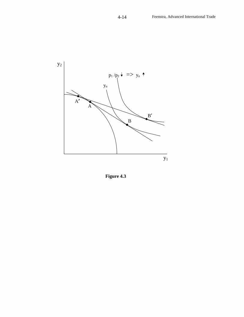
Feenstra, Advanced International Trade4-14
y2
y1
BB’
p1 /p2 => yn
Figure 4.3
yn
AA’
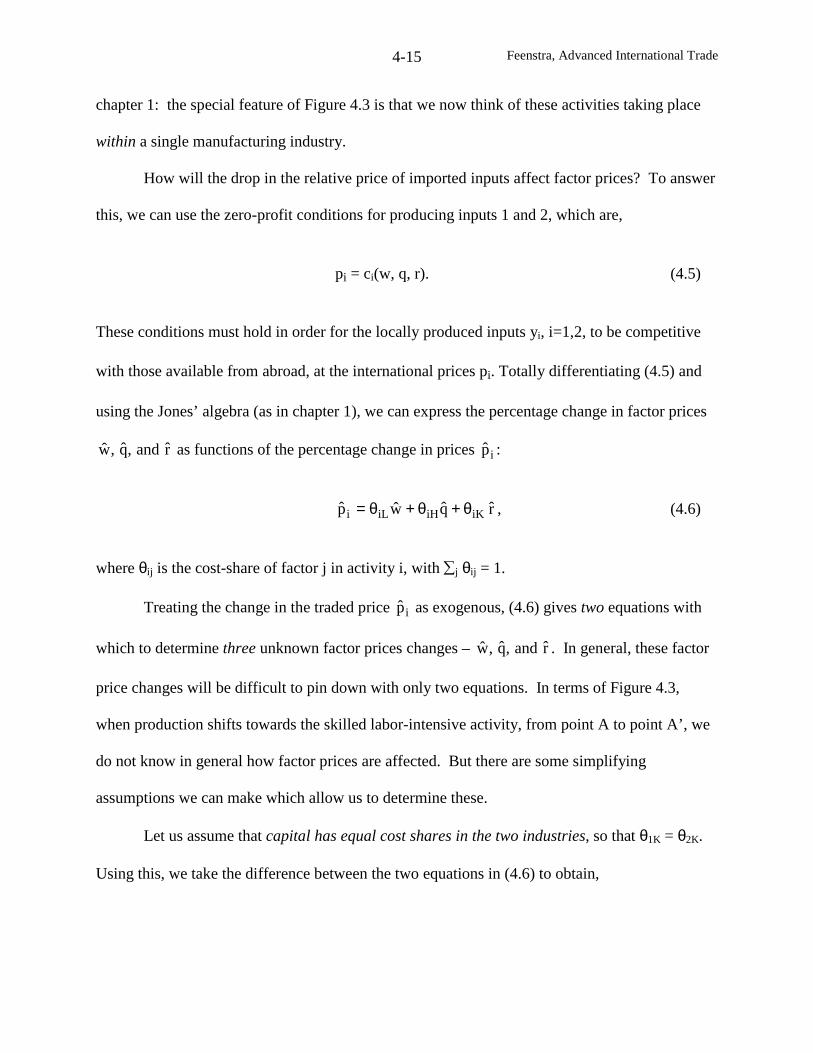
Feenstra, Advanced International Trade4-15
chapter 1: the special feature of Figure 4.3 is that we now think of these activities taking place
within a single manufacturing industry.
How will the drop in the relative price of imported inputs affect factor prices? To answer
this, we can use the zero-profit conditions for producing inputs 1 and 2, which are,
pi = ci(w, q, r). (4.5)
These conditions must hold in order for the locally produced inputs yi, i=1,2, to be competitive
with those available from abroad, at the international prices pi. Totally differentiating (4.5) and
using the Jones’ algebra (as in chapter 1), we can express the percentage change in factor prices
rand,q,w as functions of the percentage change in prices ip :
rqwp iKiHiLi θ+θ+θ= , (4.6)
where θij is the cost-share of factor j in activity i, with ∑j θij = 1.
Treating the change in the traded price ip as exogenous, (4.6) gives two equations with
which to determine three unknown factor prices changes – rand,q,w . In general, these factor
price changes will be difficult to pin down with only two equations. In terms of Figure 4.3,
when production shifts towards the skilled labor-intensive activity, from point A to point A’, we
do not know in general how factor prices are affected. But there are some simplifying
assumptions we can make which allow us to determine these.
Let us assume that capital has equal cost shares in the two industries, so that θ1K = θ2K.
Using this, we take the difference between the two equations in (4.6) to obtain,
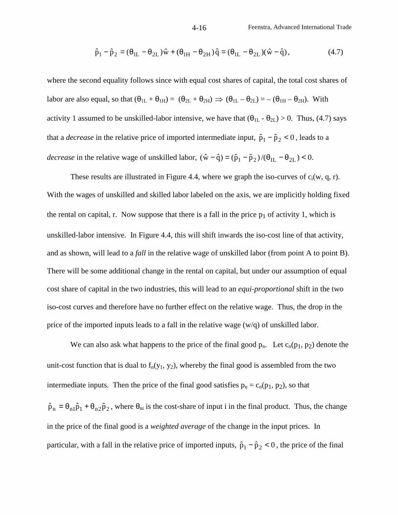
Feenstra, Advanced International Trade4-16
)qw)((q)(w)(pp L2L1H2H1L2L121 −θ−θ=θ−θ+θ−θ=− , (4.7)
where the second equality follows since with equal cost shares of capital, the total cost shares of
labor are also equal, so that (θ1L + θ1H) = (θ2L + θ2H) ⇒ (θ1L – θ2L) = – (θ1H – θ2H). With
activity 1 assumed to be unskilled-labor intensive, we have that (θ1L - θ2L) > 0. Thus, (4.7) says
that a decrease in the relative price of imported intermediate input, 0pp 21 <− , leads to a
decrease in the relative wage of unskilled labor, .0)/()pp()qw( L2L121 <θ−θ−=−
These results are illustrated in Figure 4.4, where we graph the iso-curves of ci(w, q, r).
With the wages of unskilled and skilled labor labeled on the axis, we are implicitly holding fixed
the rental on capital, r. Now suppose that there is a fall in the price p1 of activity 1, which is
unskilled-labor intensive. In Figure 4.4, this will shift inwards the iso-cost line of that activity,
and as shown, will lead to a fall in the relative wage of unskilled labor (from point A to point B).
There will be some additional change in the rental on capital, but under our assumption of equal
cost share of capital in the two industries, this will lead to an equi-proportional shift in the two
iso-cost curves and therefore have no further effect on the relative wage. Thus, the drop in the
price of the imported inputs leads to a fall in the relative wage (w/q) of unskilled labor.
We can also ask what happens to the price of the final good pn. Let cn(p1, p2) denote the
unit-cost function that is dual to fn(y1, y2), whereby the final good is assembled from the two
intermediate inputs. Then the price of the final good satisfies pn = cn(p1, p2), so that
22n11nn ppp θ+θ= , where θni is the cost-share of input i in the final product. Thus, the change
in the price of the final good is a weighted average of the change in the input prices. In
particular, with a fall in the relative price of imported inputs, 0pp 21 <− , the price of the final
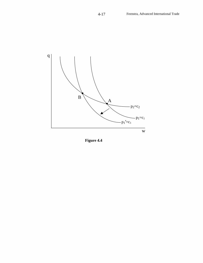
Feenstra, Advanced International Trade4-17
Ap2=c2
p1=c1
p1’=c1
B
w
q
Figure 4.4
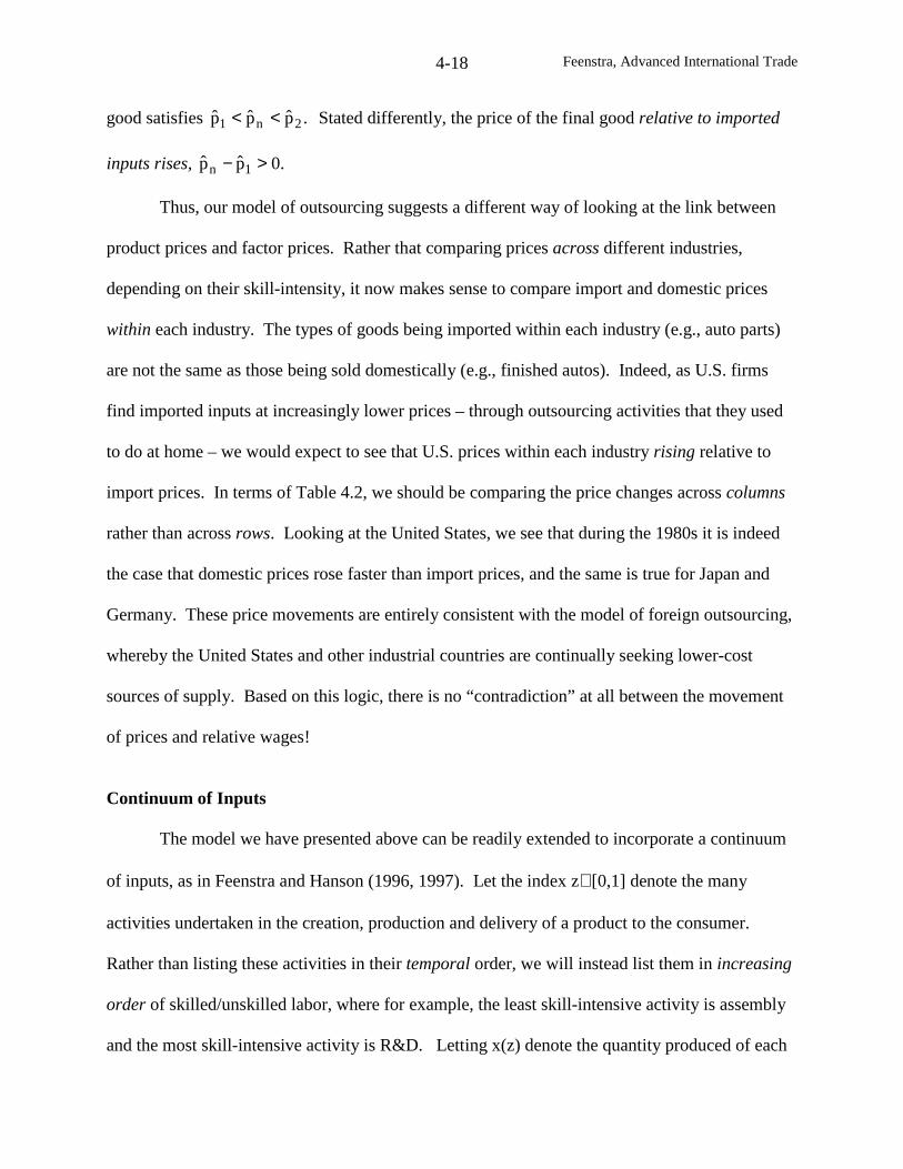
Feenstra, Advanced International Trade4-18
good satisfies .ppp 2n1 << Stated differently, the price of the final good relative to imported
inputs rises, .0pp 1n >−
Thus, our model of outsourcing suggests a different way of looking at the link between
product prices and factor prices. Rather that comparing prices across different industries,
depending on their skill-intensity, it now makes sense to compare import and domestic prices
within each industry. The types of goods being imported within each industry (e.g., auto parts)
are not the same as those being sold domestically (e.g., finished autos). Indeed, as U.S. firms
find imported inputs at increasingly lower prices – through outsourcing activities that they used
to do at home – we would expect to see that U.S. prices within each industry rising relative to
import prices. In terms of Table 4.2, we should be comparing the price changes across columns
rather than across rows. Looking at the United States, we see that during the 1980s it is indeed
the case that domestic prices rose faster than import prices, and the same is true for Japan and
Germany. These price movements are entirely consistent with the model of foreign outsourcing,
whereby the United States and other industrial countries are continually seeking lower-cost
sources of supply. Based on this logic, there is no “contradiction” at all between the movement
of prices and relative wages!
Continuum of Inputs
The model we have presented above can be readily extended to incorporate a continuum
of inputs, as in Feenstra and Hanson (1996, 1997). Let the index z∈ [0,1] denote the many
activities undertaken in the creation, production and delivery of a product to the consumer.
Rather than listing these activities in their temporal order, we will instead list them in increasing
order of skilled/unskilled labor, where for example, the least skill-intensive activity is assembly
and the most skill-intensive activity is R&D. Letting x(z) denote the quantity produced of each
Feenstra, Advanced International Trade4-19
one of these inputs, we let aH(z) and aL(z) denote the skilled and unskilled labor, respectively,
needed to produce one unit of x(z). As stated, we will order the activities z so that aH(z)/aL(z) is
non-decreasing in z.
We will suppose that there are two countries, with the foreign country denoted by an
asterisk. The production functions for producing the two inputs are assumed to be the same up to
a Hick’s-neutral productivity parameter in each country:
]1,0[z,K)z(a
)z(H,
)z(a
)z(LminA)z(x 1
HL∈
= θ−θ
. (4.8)
Thus, the amount of skilled and unskilled labor H(z) and L(z) are used in the home country to
produce input z, using a Leontief technology between these two types of labor, and then a Cobb-
Douglas technology between labor overall and capital K. The parameter θ denotes the share of
labor in the costs of producing each input. The foreign production function is the same, except
with a different productivity parameter A*.
Rather than working with the production functions for the inputs in (4.8), it will be
convenient to work with the dual unit-cost function:
,r)]z(qa)z(wa[B)z,r,q,w(c 1iHL
θ−θ+= (4.9)
where c(w,q,r,z) denotes the costs of producing one unit of x(z) in the home country, given the
wage of unskilled labor w, the wage of skilled labor q, and the rental on capital r. The inputs
can be produced in either country, and are then combined into the production of a final product.
The production function for the final good is assumed to be a Cobb-Douglas function over all the
inputs:
Feenstra, Advanced International Trade4-20
∫∫ =αα=1
0
1
01dz)z(with,dz)z(xln)z(Yln . (4.10)
Notice that in (4.10) we have not included labor as an input, so the final good is assembled
“costlessly” from all the individual inputs z∈ [0,1]. This means that we do not need to keep
track of which country the assembly takes place, because there is zero value-added (and zero
demand for labor) in this activity.
In general, firms doing the assembly will wish to source the inputs from the minimum
cost location. To determine this, we will make the following assumption on factor prices:
*rrand,*w
*q
w
q << . (4.11)
The first assumption in (4.11) states that the relative wage of skilled labor is lower at home than
abroad, which is realistic if the home country is skilled-labor abundant, like the U.S.: despite the
increase in the relative wage of skilled labor in the United States during the past two decades, it
is still much lower than in Mexico. The second assumption states that the rental on capital is
lower at home, so that if capital is able to move, it will want to re-locate abroad. This is also
realistic if the home country is capital abundant, and will provide the basis for some comparative
statics we shall consider.
With assumption (4.11), we can graphically illustrate the problem of choosing the
minimum cost location for each input. Let us begin by graphing the unit-costs (4.9) for the home
country, given fixed factor prices. The unit-costs c(w,q,r,z) as a function of z can have any shape
whatsoever, and need not even be a continuous function. For convenience, however, we will
assume that it is continuous, and illustrate this function as the upward-sloping curve CC in
Feenstra, Advanced International Trade4-21
Figure 4.5. Then the question is: how does the locus of unit-costs c*(w*,q*, r*,z) abroad,
which we denote by C*C* related to that at home?
If the unit-costs of all activities were lower at home, for example, then all inputs would
be produced there, and vice-versa if all unit-costs are lower abroad. We are interested in the case
where there is some “production sharing” across the countries, so assume that the curves C*C*
and CC intersect at least once, and denote this input by z*, with c(w,q,r,z*) = c(w*,q*,r*,z*).
Then consider an activity z’ > z* with slightly higher skilled/unskilled labor requirements.
Because of our assumptions that (q/w) < (q*/w*), the higher skilled/unskilled requirements
should have a greater impact on foreign costs than on home costs. We therefore expect that
c(w,r,q,z’) < c(w*,q*,r*,z’) for z’ > z*. Similarly, we expect that the converse is also true,
c(w,q,r,z’) > c(w*,q*,r*,z’) for z’ < z*. Thus, the loci C*C* and CC can intersect at most once,
as shown in Figure 4.5.11 The similarity of this analysis with the model of Dornbusch, Fisher
and Samuelson (1980) in the previous chapter will be clear to the reader, where we used nearly
the same diagrams.
Given this unique intersection, we see that foreign unit-costs are less than those at home
for all z’ < z*, so that the foreign country will specialize in the products [0, z*), whereas home
unit-costs are less than those abroad for all z’ > z*, so the home country will specialize in (z*, 1].
Using this information, we can then calculate the demand for labor in each country. At home,
for example, the relative demand for skilled/unskilled labor is:
∫
∫
∂∂∂∂
=1
*z
1
*z
dz)z(xw
c
dz)z(xq
c
*)z(D . (4.12)
11 This is proved by Feenstra and Hanson (1996).
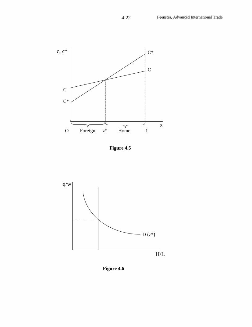
Feenstra, Advanced International Trade4-22
D (z*)
H/L
q/w
Figure 4.6
z
C*
C
C
C*
O Foreign z* Home 1
Figure 4.5
c, c*
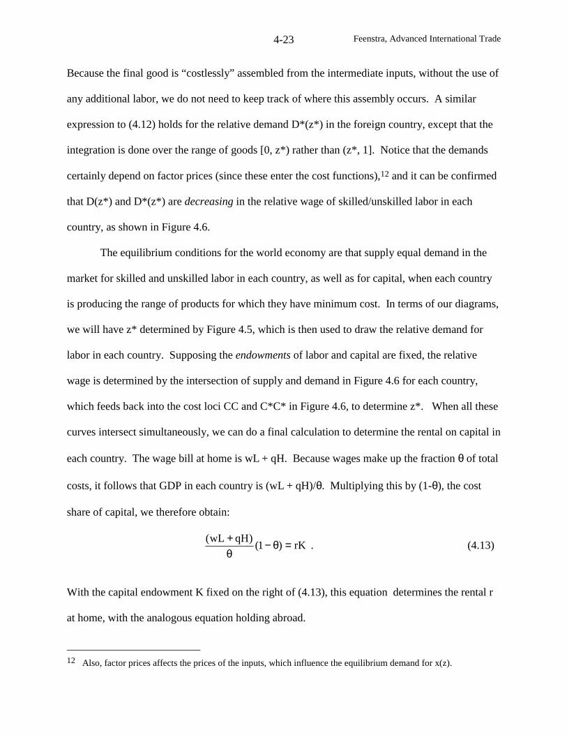
Feenstra, Advanced International Trade4-23
Because the final good is “costlessly” assembled from the intermediate inputs, without the use of
any additional labor, we do not need to keep track of where this assembly occurs. A similar
expression to (4.12) holds for the relative demand D*(z*) in the foreign country, except that the
integration is done over the range of goods [0, z*) rather than (z*, 1]. Notice that the demands
certainly depend on factor prices (since these enter the cost functions),12 and it can be confirmed
that D(z*) and D*(z*) are decreasing in the relative wage of skilled/unskilled labor in each
country, as shown in Figure 4.6.
The equilibrium conditions for the world economy are that supply equal demand in the
market for skilled and unskilled labor in each country, as well as for capital, when each country
is producing the range of products for which they have minimum cost. In terms of our diagrams,
we will have z* determined by Figure 4.5, which is then used to draw the relative demand for
labor in each country. Supposing the endowments of labor and capital are fixed, the relative
wage is determined by the intersection of supply and demand in Figure 4.6 for each country,
which feeds back into the cost loci CC and C*C* in Figure 4.6, to determine z*. When all these
curves intersect simultaneously, we can do a final calculation to determine the rental on capital in
each country. The wage bill at home is wL + qH. Because wages make up the fraction θ of total
costs, it follows that GDP in each country is (wL + qH)/θ. Multiplying this by (1-θ), the cost
share of capital, we therefore obtain:
rK)1()qHwL( =θ−
θ+
. (4.13)
With the capital endowment K fixed on the right of (4.13), this equation determines the rental r
at home, with the analogous equation holding abroad.
12 Also, factor prices affects the prices of the inputs, which influence the equilibrium demand for x(z).
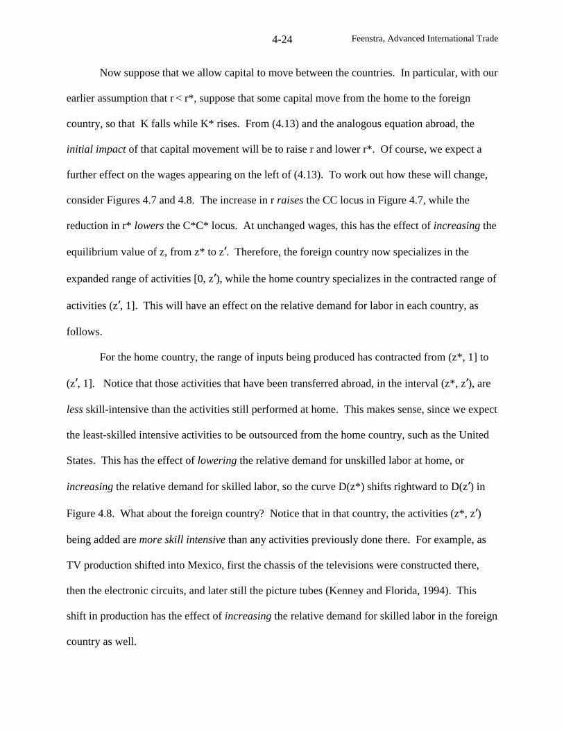
Feenstra, Advanced International Trade4-24
Now suppose that we allow capital to move between the countries. In particular, with our
earlier assumption that r < r*, suppose that some capital move from the home to the foreign
country, so that K falls while K* rises. From (4.13) and the analogous equation abroad, the
initial impact of that capital movement will be to raise r and lower r*. Of course, we expect a
further effect on the wages appearing on the left of (4.13). To work out how these will change,
consider Figures 4.7 and 4.8. The increase in r raises the CC locus in Figure 4.7, while the
reduction in r* lowers the C*C* locus. At unchanged wages, this has the effect of increasing the
equilibrium value of z, from z* to z’. Therefore, the foreign country now specializes in the
expanded range of activities [0, z’), while the home country specializes in the contracted range of
activities (z’, 1]. This will have an effect on the relative demand for labor in each country, as
follows.
For the home country, the range of inputs being produced has contracted from (z*, 1] to
(z’, 1]. Notice that those activities that have been transferred abroad, in the interval (z*, z’), are
less skill-intensive than the activities still performed at home. This makes sense, since we expect
the least-skilled intensive activities to be outsourced from the home country, such as the United
States. This has the effect of lowering the relative demand for unskilled labor at home, or
increasing the relative demand for skilled labor, so the curve D(z*) shifts rightward to D(z’) in
Figure 4.8. What about the foreign country? Notice that in that country, the activities (z*, z’)
being added are more skill intensive than any activities previously done there. For example, as
TV production shifted into Mexico, first the chassis of the televisions were constructed there,
then the electronic circuits, and later still the picture tubes (Kenney and Florida, 1994). This
shift in production has the effect of increasing the relative demand for skilled labor in the foreign
country as well.
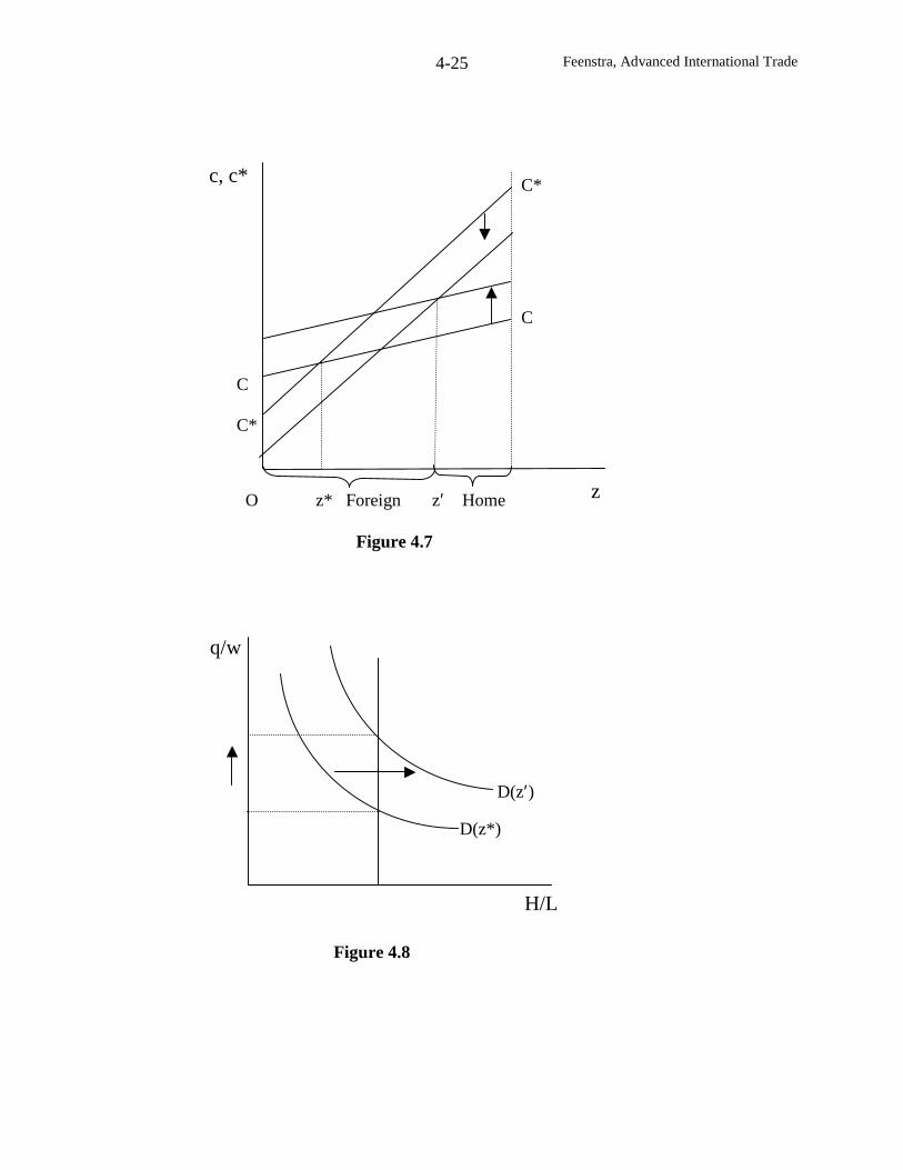
Feenstra, Advanced International Trade4-25
O z* Foreign z′ Home
Figure 4.7
C*
C
D(z′)
D(z*)
H/L
Figure 4.8
q/w
c, c*
C
C*
z
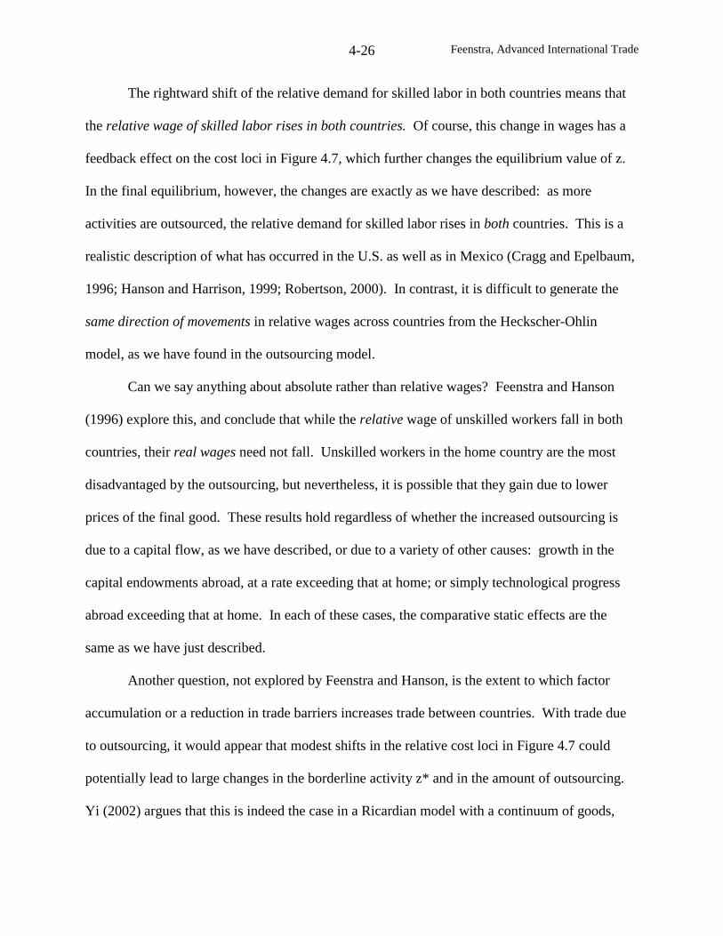
Feenstra, Advanced International Trade4-26
The rightward shift of the relative demand for skilled labor in both countries means that
the relative wage of skilled labor rises in both countries. Of course, this change in wages has a
feedback effect on the cost loci in Figure 4.7, which further changes the equilibrium value of z.
In the final equilibrium, however, the changes are exactly as we have described: as more
activities are outsourced, the relative demand for skilled labor rises in both countries. This is a
realistic description of what has occurred in the U.S. as well as in Mexico (Cragg and Epelbaum,
1996; Hanson and Harrison, 1999; Robertson, 2000). In contrast, it is difficult to generate the
same direction of movements in relative wages across countries from the Heckscher-Ohlin
model, as we have found in the outsourcing model.
Can we say anything about absolute rather than relative wages? Feenstra and Hanson
(1996) explore this, and conclude that while the relative wage of unskilled workers fall in both
countries, their real wages need not fall. Unskilled workers in the home country are the most
disadvantaged by the outsourcing, but nevertheless, it is possible that they gain due to lower
prices of the final good. These results hold regardless of whether the increased outsourcing is
due to a capital flow, as we have described, or due to a variety of other causes: growth in the
capital endowments abroad, at a rate exceeding that at home; or simply technological progress
abroad exceeding that at home. In each of these cases, the comparative static effects are the
same as we have just described.
Another question, not explored by Feenstra and Hanson, is the extent to which factor
accumulation or a reduction in trade barriers increases trade between countries. With trade due
to outsourcing, it would appear that modest shifts in the relative cost loci in Figure 4.7 could
potentially lead to large changes in the borderline activity z* and in the amount of outsourcing.
Yi (2002) argues that this is indeed the case in a Ricardian model with a continuum of goods,
Feenstra, Advanced International Trade4-27
and that “vertical specialization” accounts for more than 50% of the growth in U.S. trade since
1962. This paper is recommended for further reading.
Estimating the Relative Demand for Skilled Labor
Summarizing our argument so far, the decision of companies to purchase intermediate
inputs from overseas will most certainly affect their employment at home, and can be expected to
differentially affect skilled versus unskilled workers. With firms in industrial countries facing a
higher relative wage for unskilled labor than that found abroad, the activities that are outsourced
would be those that use a large amount of unskilled labor, such as assembly of components and
other repetitive tasks. Moving these activities overseas will reduce the relative demand for
unskilled labor in the industrial country, in much the same way as replacing these workers with
automated production. This means that outsourcing has a qualitatively similar effect on
reducing the relative demand for unskilled labor within an industry as does skilled-biased
technological change, such as the increased use of computers. Thus, determining which of these
is most important is an empirical question.
We will examine two methods that have been used to estimate the effects of trade versus
technological change on wages and employment. The first method estimates the demand for
skilled and unskilled labor. Let us return to the simple three-good, three-factor model introduced
above, where we derived the revenue function Gn(Ln, Hn, Kn, pn, p) in (4.4) for each industry
n=1,…,N, where p = (p1,p2) is the vector of imported input prices. It will be convenient to work
with a “short-run” cost function that is dual to (4.4). Note that the function Gn(Ln, Hn, Kn, pn, p)
is linearly homogeneous in prices, so we can alternatively write it as pnGn(Ln, Hn, Kn, 1, p/ pn).
Thus, a natural measure of real value-added is,
Feenstra, Advanced International Trade4-28
Yn = Gn(Ln, Hn, Kn, 1, p/pn) . (4.14)
This measure of output is nearly the same as yn, except it now includes real net exports.
Provided that the underlying production functions fi, i=1,2,n, are increasing and concave, then
the function Gn will also be increasing and concave in (Ln, Hn, Kn).
Then the short-run cost function, obtained when the level of capital and output are fixed,
is defined as:
Cn(w, q, Kn, Yn, p/pn) ≡nn H,L
min wLn + qHn , subject to (4.14). (4.15)
Notice that we have included the relative price of traded inputs p/pn in this cost function since
they also appear in the revenue function (4.14). More generally, any structural variables that
shift the production function and therefore affect costs should be included as arguments. In the
model discussed above with a continuum of input, the range of inputs imported into each country
should appear as an argument in (4.15). That is, it is not enough to just keep track of import
prices – we also need to keep track of newly imported intermediate inputs. In practice, we will
measure this by the expenditure on imported inputs for each industry, though this does not fully
capture the idea of newly imported inputs.13 We will denote all such variables that affect costs
in industry n by the vector zn; in addition to imported inputs, this can include expenditures on
computers and other new types of capital equipment. We therefore rewrite the cost function in
(4.15) as Cn(w, q, Kn, Yn, zn).
13 In chapter 10 we discuss methods to directly measure the product variety of imports. Dinopoulos andSegerstrom (1999), Zhu (2000a) and Zhu and Trefler (2001) develop models that emphasize the link between newvarieties of traded goods and wages, with corresponding empirical work by Zhu (2000b). These papers arerecommended for further reading.
Feenstra, Advanced International Trade4-29
The next step is to choose a functional form for costs. As in our discussion of the GDP
function in chapter 3, a convenient choice is the translog cost function, which is written in a
general notation (dropping the industry subscript n) as,
k
M
1i
K
1kiik
K
1k
K
1kk2
1
j
M
1i
M
1jiij
M
1i
K
1k2
1kkii0
xlnwlnxlnxln
wlnwlnxlnwlnCln
∑∑∑∑
∑∑∑ ∑
= == =
= == =
φ+δ+
γ+β+α+α=
ll
l
(4.16)
where wi denotes the wages of the optimally chosen inputs i=1,…,M, and xk denotes either the
quantities of the fixed inputs or outputs k=1,…,K, or any other shift parameters.14 In terms of the
cost function in (4.15), there are just two optimally chosen factors – skilled and unskilled labor –
while capital and output are treated as fixed in the short run.
The usefulness of the translog function comes from computing its first derivatives,
∂lnC/∂lnwi = (∂C/∂wi)(wi/C). Because ∂C/∂wi equals the demand for the chosen input i, it
follows that (∂C/∂wi)(wi/C) equals the payments to factor i relative to total costs, which we
denote by the cost-shares si. Thus, differentiating (4.16) with respect to ln wi , we obtain,
k
K
1kik
M
1jjijii xlnwlns ∑∑
==φ+γ+α= , i=1,…,M. (4.17)
Given annual data on factor cost shares, wages, and fixed inputs and outputs, this set of linear
equations can be estimated over time for a given industry to obtain the coefficients γij and φik.15
14 Without loss of generality we impose the symmetry requirement that γij = γji. In addition, to ensure that the
translog cost function is homogeneous of degree one in wages, we impose .0and1M
1i ikM
1i ijM
1i i =φ=γ=α ∑∑∑ ===15 Generally, the dependent variables in the system (4.17) sum to unity, which means that one of the equations canbe derived from the others. Under these conditions, one of the equations is dropped before the system is estimated.
Feenstra, Advanced International Trade4-30
Alternatively, the equations can be estimated for a single year, or the change between two years,
by pooling data across industries. In the latter case, we are assuming that the same cost function
applies across the industries. Despite this strong assumption, the cross-industry approach is
popular and we will follow it here.
Returning now to the notation Cn(w, q, Kn, Yn, zn) as in (4.15), we have two chosen
inputs – skilled and unskilled labor. Focusing on the share equation for skilled labor, it will
depend on wages for both types of labor, as well capital, output, and all other structural variables,
zn. When (4.17) is estimated by pooling data across industries, as in Berman, Bound and
Griliches (1994) for example, it is felt the cross-industry variation in wages has little
information: wages differ across industries principally due to quality-variation of workers, so we
do not expect high-wage industries to economize on those (high-quality) workers. Accordingly,
the wage terms are typically dropped from the right of (4.17) when pooling data across
industries. This leaves just fixed capital, output, and other structural variables. Taking the
difference between two years, the estimating equation for the wage-share of skilled labor (snH) in
industries n=1,…,N becomes:
nznYnK0nH z'YlnKlns ∆φ+∆φ+∆φ+φ=∆ , n=1,…,N, (4.18)
where zn denotes the vector of structural variables that shifts costs, and φz is the corresponding
vector of coefficients. In particular, when the wage-share of skilled labor is increasing, we are
interested in determining how much of that increase is due to changes in capital, output, and the
structural variables.
Estimates of (4.18) for 447 industries within the U.S. manufacturing sector, over 1979-
1990, are shown in Table 4.4. The data are from the NBER Productivity Database (Bartelsman
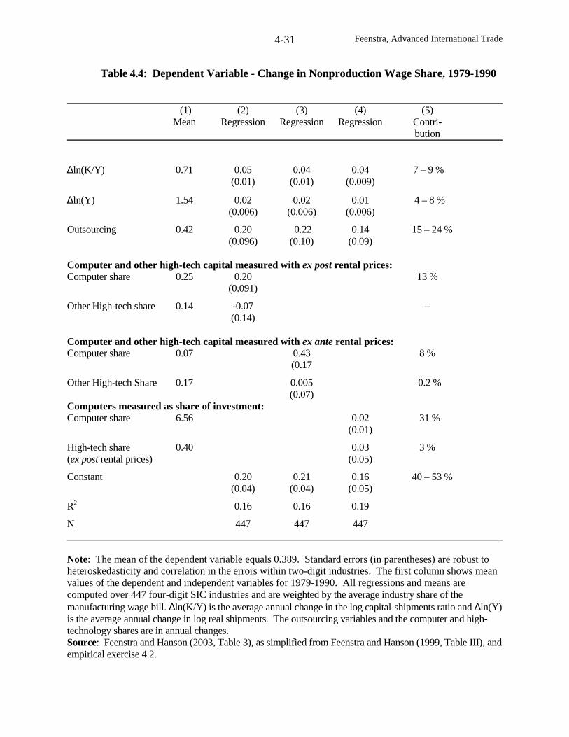
Feenstra, Advanced International Trade4-31
Table 4.4: Dependent Variable - Change in Nonproduction Wage Share, 1979-1990
(1) (2) (3) (4) (5)Mean Regression Regression Regression Contri-
bution
∆ln(K/Y) 0.71 0.05 0.04 0.04 7 – 9 %(0.01) (0.01) (0.009)
∆ln(Y) 1.54 0.02 0.02 0.01 4 – 8 %(0.006) (0.006) (0.006)
Outsourcing 0.42 0.20 0.22 0.14 15 – 24 %(0.096) (0.10) (0.09)
Computer and other high-tech capital measured with ex post rental prices:Computer share 0.25 0.20 13 %
(0.091)
Other High-tech share 0.14 -0.07 --(0.14)
Computer and other high-tech capital measured with ex ante rental prices:Computer share 0.07 0.43 8 %
(0.17
Other High-tech Share 0.17 0.005 0.2 %(0.07)
Computers measured as share of investment:Computer share 6.56 0.02 31 %
(0.01)
High-tech share 0.40 0.03 3 %(ex post rental prices) (0.05)
Constant 0.20 0.21 0.16 40 – 53 %(0.04) (0.04) (0.05)
R2 0.16 0.16 0.19
N 447 447 447
Note: The mean of the dependent variable equals 0.389. Standard errors (in parentheses) are robust toheteroskedasticity and correlation in the errors within two-digit industries. The first column shows meanvalues of the dependent and independent variables for 1979-1990. All regressions and means arecomputed over 447 four-digit SIC industries and are weighted by the average industry share of themanufacturing wage bill. ∆ln(K/Y) is the average annual change in the log capital-shipments ratio and ∆ln(Y)is the average annual change in log real shipments. The outsourcing variables and the computer and high-technology shares are in annual changes.Source: Feenstra and Hanson (2003, Table 3), as simplified from Feenstra and Hanson (1999, Table III), andempirical exercise 4.2.
Feenstra, Advanced International Trade4-32
and Gray, 1996, which is available at http://www.nber.org/nberces/ ).16 In these regressions we
use nonproduction labor as a proxy for skilled labor, so the dependent variable is the change in
the share of nonproduction labor in total wages within each industry. Over all manufacturing
industries, the nonproduction wage share increased from 35.4% to 42.4% between 1979 and
1990, for an annual growth of 0.4% (four-tenths of one percent) per year. It is common to weight
regressions like those in Table 4.4 by the industry share of the total manufacturing wage bill, as we
shall do. In this way, large industries receive more weight in the regressions. The regressors
included are: the shipments of each industry (as a proxy for real value-added Yn); the
capital/shipments ratio (reflecting the capital input Kn relative to Yn); outsourcing, measured by
imported intermediate inputs as a share of total intermediate purchases (one of the zn variables);
and the share of computers and other high-tech capital in the capital stock (other zn variables).
Several of these variables deserve further explanation.
The imported intermediate inputs have been estimated by Feenstra and Hanson (1999)
using the input-output matrix of the U.S. economy, combined with trade data. For example, if
the automobile industry purchases 10% of its inputs from the steel industry, and 30% of steel
consumed in the U.S. is imported, then we conclude that 3% of the inputs in autos is due to
imported steel. This is summed over all intermediate inputs to arrive at the overall share of
imported inputs for each industry. The share of computers and other high-tech capital in the
capital stock is constructed in three different ways: first, using ex post rental prices to measure
capital services; second, using ex ante rental prices to measure capital services;17 and third, by
16 In empirical exercise 4.1, you are asked to download this dataset and reproduce Figures 4.1-4.2, and in exercise4.2 you are asked to reproduce Table 4.4.17 To explain the construction of rental prices, suppose that there is only one type of capital and labor, so that
value-added in an industry is pYn = wLn + rKn. Given data on sales and on compensation to labor, the ex post
Feenstra, Advanced International Trade4-33
measuring computer expenditures as a share of investment rather than of the capital stock.18 We
think that it is preferable to measure the contribution of computers to the capital stock, rather
than to new investment, but experiment with all three approaches.
In column (1) of Table 4.4, we report the mean values of the dependent and independent
variables for 1979-1990, and, following this, the regression coefficients in columns (2)-(4). Each
regression uses alternative measures of the computer and other high-technology shares. In all the
regressions, we see that outsourcing has a positive impact on the nonproduction share of the
wage bill, as does the computer share. By multiplying the regression coefficients by the mean
values for the change in each variable, we obtain the contributions of each to the total change in
the nonproduction wage share, shown in column (5). We see that outsourcing accounts for 15%-
24% of the shift towards nonproduction labor.
The results for computers depend on the specification. Measuring computer services and
other high-tech capital as a share of the capital stock using ex post rental prices, we see they
account for 13% of the shift towards nonproduction labor. Measuring these shares using ex ante
rental prices, we see that that computers and other high-tech capital explain only 8% of this shift.
payments to capital are constructed as a residual, rKn = pYn – wLn. Next, we need some measure of the physical
capital stock Kn, which is typically constructed from investment data In using the perpetual inventory method:
Knt = (1–δ)Knt-1 + Int, where δ is a depreciation rate for capital. Then using the constructed physical capital in yeart, and the total payments to capital in year t, these are divided to obtain the ex post rental on capital in year t:
rt = (pYnt – wLnt)/Knt. Then using the purchase price of capital pkt, the implied ex post rate of return to capital
would be constructed as ρt = (rt /pkt) – δ + [( pkt+1 – pkt)/ pkt]. Thus, the ex post rate of return includes the rentalrelative to the purchase price, minus depreciation, plus any capital gains or losses on the capital equipment. Incontrast, an ex ante rate of return would ignore the capital gains or losses. Thus, if we chose ρ* as a “safe” rate ofreturn such as on a bond, then the corresponding ex ante rental price would be obtained by ignoring capital gains and
computing rt from the equation, rt = (ρ* + δ)pkt . The formulas used for the rental prices becomes morecomplicated when we take into account business taxes, and when there are multiple types of capital. For furtherdetails see Harper, Berndt and Wood (1989).18 The share of computer spending in investment is obtained from the Census of Manufactures, which simply askedfirms to report what percentage of new investment was devoted to computers. This variable has been used previously byBerman, Bound and Griliches (1994) and Autor, Katz and Krueger (1998).
Feenstra, Advanced International Trade4-34
In both cases, the contribution of computers and other high-tech capital is less than the
contribution of outsourcing. In contrast, when computers are measured by their share of
investment (and the high-technology capital share is also included), we see that these variables
account for 31% of the shift toward nonproduction labor, which exceeds the contribution of
outsourcing. Thus, whether outsourcing is more or less important than computers depends on
whether the latter are measured as a share of the capital stock, or as a share of investment.
Regardless of the specification, however, it is fair to conclude that both outsourcing and
expenditure on computers and other high technology capital are important explanations of the
shift towards nonproduction labor in the U.S., with their exact magnitudes depending on how
they are measured.
A specification like (4.18) has also been used to investigate the demand shift towards
nonproduction labor in various other countries. Following its liberalization of foreign
investment and trade in the 1980s, Mexico experienced an increase in the relative wage of skilled
labor (Hanson and Harrison, 1999). In the period following reform, foreign direct investment
(FDI) in Mexico was concentrated in foreign assembly plants, known as maquiladoras, most of
which are located in Mexican states along the U.S. border. These assembly plants are created, in
most cases, by U.S. firms outsourcing unskilled-labor intensive production activities to Mexico.
Feenstra and Hanson (1997) find that the shift in Mexican manufacturing towards foreign
assembly plants over 1975-1988 can account for 45% of the increase in the country’s
nonproduction wage share. Evidence supporting the link between outsourcing or import
penetration and wages shares or relative employment is also available for Austria (Dell’mour et
al, 2000), Germany (Geishecker, 2002), Hong Kong (Hsieh and Woo, 1999), Japan (Head and
Ries, 2002) and the U.K. (Anderton and Brenton, 1999; and Görg, et al 2001).
Feenstra, Advanced International Trade4-35
In the specification (4.18), outsourcing changes the relative wage by shifting out the
relative demand for skilled labor. An alternative view is that international trade changes factor
prices by flattening the labor demand curves, making them more elastic. Leamer (1998) presents
an extreme version of this story, in which the transition of an economy from autarky to trade
transforms an economy’s labor demand curve from being downward sloping to being horizontal,
at least over segments that correspond to diversified production.19 Extending this logic, Rodrik
(1997) identifies several mechanism through which greater economic integration between
countries may make labor demand curves flatter. In one of the few attempts to test this
hypothesis, Slaughter (2001) estimates the own-price elasticity of labor demand for production
and nonproduction workers in two-digit U.S. manufacturing industries over the period 1960-
1991. Over the entire sample, demand became more elastic for production labor, but not for
nonproduction labor. The sectors with the largest increase in elasticities were food and tobacco,
apparel and textiles, wood and paper, and primary and fabricated metals, which include some of
the least-skill intensive manufacturing industries. The demand for production labor became
more elastic in industries with more outsourcing, more investment in computers, and more
investment in high-tech capital overall. These results are robust to controls for industry fixed
effects but not time fixed effects, suggesting that changes in labor-demand elasticities are
dominated by a time trend.
Estimating the Zero Profit Conditions
The second empirical technique we will discuss assumes that both types of labor, as well
as capital, are being optimally chosen. So we abandon the “short run” cost function in (4.15),
and instead use the more familiar long-run cost function for the industry:
19 See problem 4.1.
Feenstra, Advanced International Trade4-36
Cn(wn, qn, rn, Yn, p/pn) ≡nnn K,H,L
min wnLn + qnHn + rnKn, subject to (4.14). (4.19)
Notice that in (4.19) we have allowed the factor prices wn, qn, and rn to differ across the
industries n=1,…,N. This reflects the empirical fact that factor prices, and wages in particular,
do differ across industries (Krueger and Summers, 1988), and will turn out to be important. As
before, the relative price of traded inputs p/pn enters this cost function because it also appears in
the revenue function (4.14); we will replace this by the vector zn, which includes other structural
variables.
Since the revenue function (4.14) is linearly homogeneous in inputs, then we can rewrite
the cost function in (4.19) as,
Cn(wn, qn, rn, Yn, zn) = Yn cn(wn, qn, rn, zn) , (4.20)
where cn(wn, qn, rn, zn) denotes the unit-cost function. The zero-profit conditions in the industries
are therefore expressed as,
pn = cn(wn, qn, rn, zn), n=1,…,N . (4.21)
Throughout this book, we have examined how changes in product prices affect factor
prices. Now, however, the presence of the structural variables zn means that the changes in
prices reflect more than just changes in factor prices. Indeed, taking the difference between the
log change in factor and product prices, we can define total factor productivity as,
nnnKnnHnnLn pln)rlnqlnwln(TFP ∆−∆θ+∆θ+∆θ≡ , (4.22)
where the cost-shares of the three factors sum to unity, θnL + θnH + θnK = 1, and ∆ denotes the
first-difference. Productivity improvements mean that factor prices rise more than product
Feenstra, Advanced International Trade4-37
prices, so that (4.22) is positive. Note that this is the “dual” definition of productivity, and
empirically it is very close to the “primal” definition, which is the growth in output minus the
weighted average of the growth in inputs.20
Shuffling the terms in (4.22) slightly, we obtain the equation,
nnKnnHnnLnn rlnqlnwlnTFPpln ∆θ+∆θ+∆θ+−=∆ , n=1,…,N. (4.23)
We consider estimating (4.23) as a linear regression across industries, where the data are the
change in log prices, total factor productivity, and the factor cost-shares θnj, while the change in
factor-prices are estimated as regression coefficients. That is, we estimate the implied change in
factor-prices βL, βH, and βK from the regression:
nKnKHnHLnLnn TFPpln ε+βθ+βθ+βθ+−=∆ , n=1,…,N, (4.24)
where εn is an error term, specified more fully below. We interpret the coefficients βL, βH, and
βK as the change in factor prices that are “mandated by” the change in product prices, which is
the dependent variable in (4.24). We hope to find that the estimate factor prices changes βL, βH,
and βK from this regression are quite close to their actual changes, and if so, we can conclude
that a Stolper-Samuelson linkage between product and factor prices works empirically. Baldwin
and Hilton (1984) were among the first to estimate this price regression, and there are many
recent applications of it (Baldwin and Cain, 2000, Slaughter, 2000), as discussed below.
20 That is, the primal definition of productivity is )KlnHlnLln(nYlnTFP nnKnnHnnLn ∆θ+∆θ+∆θ−∆≡ . With
the log change in quantities or prices measured between two years, we should construct the factor cost-shares as theaverage of the cost-shares in the two years. This formulation is called the Tornqvist index of productivity, and willbe discussed further in chapter 10, and in Appendix A.
Feenstra, Advanced International Trade4-38
Estimates of (4.24) for 447 U.S. manufacturing industries, over 1979-1990, are provided
in Table 4.5. The dependent variable is the log change in the industry output price over the
period, and we use the primal measure of TFP. The other independent variables are the average
cost-shares for production labor, nonproduction labor, and capital; the materials cost share times
the log change in materials prices; and the energy cost share times the log change in energy
prices. Note that we do not attempt to estimate the change in materials prices and energy prices,
but simply include these cost shares times their prices as controls.
In columns (1) and (2), we constrain the coefficients on the materials share times the
materials price, and the energy share times the energy price, to be unity. This approximates the
specification in Leamer (1998). In column (1), the coefficients on the labor shares imply a
decrease in the nonproduction/production relative wage of 2.3% – 3.1% = –0.8% per year, which
is consistent with the results in Leamer (1998). But in reality, the nonproduction-production
wage gap in the U.S. rose by 0.7% per year, or about seven-tenths of one percent.21 So the
regression in column (1) does not reproduce at all the actual factor prices changes in the United
States! In column (2), we follow Sachs and Shatz (1994) and drop the computer industry (SIC
3573), which reverses the predicted change in wage inequality. Now, nonproduction wages are
mandated to rise by 1.5% per year more than production wages. In column (3), we approximate
Krueger’s (1997) specification by dropping TFP as a regressor, while estimating coefficients on
materials and energy. There is again a mandated rise in the nonproduction-production wage gap,
but one that is much larger than the actual increase in relative wages.
21 After weighted by each industry’s share of manufacturing shipments, the average nominal wages of non-production workers rose by 5.4% per year over 1979-1990, and the nominal wages of production workers rose by4.7% per year. The difference between these, 0.7%, is the increasing “wage gap” that needs to be explained.
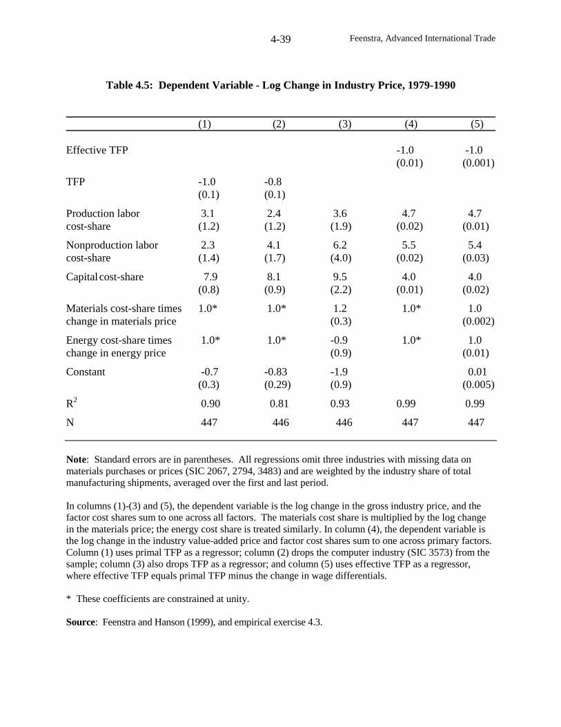
Feenstra, Advanced International Trade4-39
Table 4.5: Dependent Variable - Log Change in Industry Price, 1979-1990
(1) (2) (3) (4) (5)
Effective TFP -1.0 -1.0(0.01) (0.001)
TFP -1.0 -0.8(0.1) (0.1)
Production labor 3.1 2.4 3.6 4.7 4.7cost-share (1.2) (1.2) (1.9) (0.02) (0.01)
Nonproduction labor 2.3 4.1 6.2 5.5 5.4cost-share (1.4) (1.7) (4.0) (0.02) (0.03)
Capitalcost-share 7.9 8.1 9.5 4.0 4.0(0.8) (0.9) (2.2) (0.01) (0.02)
Materials cost-share times 1.0* 1.0* 1.2 1.0* 1.0change in materials price (0.3) (0.002)
Energy cost-share times 1.0* 1.0* -0.9 1.0* 1.0change in energy price (0.9) (0.01)
Constant -0.7 -0.83 -1.9 0.01(0.3) (0.29) (0.9) (0.005)
R2 0.90 0.81 0.93 0.99 0.99
N 447 446 446 447 447
Note: Standard errors are in parentheses. All regressions omit three industries with missing data onmaterials purchases or prices (SIC 2067, 2794, 3483) and are weighted by the industry share of totalmanufacturing shipments, averaged over the first and last period.
In columns (1)-(3) and (5), the dependent variable is the log change in the gross industry price, and thefactor cost shares sum to one across all factors. The materials cost share is multiplied by the log changein the materials price; the energy cost share is treated similarly. In column (4), the dependent variable isthe log change in the industry value-added price and factor cost shares sum to one across primary factors.Column (1) uses primal TFP as a regressor; column (2) drops the computer industry (SIC 3573) from thesample; column (3) also drops TFP as a regressor; and column (5) uses effective TFP as a regressor,where effective TFP equals primal TFP minus the change in wage differentials.
* These coefficients are constrained at unity.
Source: Feenstra and Hanson (1999), and empirical exercise 4.3.
Feenstra, Advanced International Trade4-40
The estimates in Table 4.5 are troubling because they show that slight changes in the
data, such as dropping the computer industry, have dramatic effects on the results. While it is
true that the computer industry is an outlier, the sensitivity of the results to the specification
suggests that something more basic is going on. To address this, let us ask: why do the
estimates of βL, βH, and βK from regression (4.24) differ at all from the actual average change in
manufacturing wages, which we denote by rlnand,qln,wln ∆∆∆ ? The overbar indicates that
we are averaging the change in factor-prices over all manufacturing industries. By just
comparing (4.23) and (4.24), it seems that there should be some close connection between the
estimates βL, βH, and βK and these average actual factor price changes, but we need to uncover
what this connection is.
To achieve this, let us make the transition from (4.23) to an estimating equation more
carefully. First, notice that we can rewrite (4.23) as,
nnKnHnLnn rlnqlnwlnTFPpln ε+∆θ+∆θ+∆θ+−=∆ , (4.25)
where,
)rlnrln()qlnqln()wlnwln( nnKnnHnnLn ∆−∆θ+∆−∆θ+∆−∆θ≡ε . (4.26)
That is, we replace the industry wage changes on the right of (4.23) by the average wage
changes, and incorporate the difference between these two into an error term. In economic
terms, εn reflects interindustry wage differentials: i.e., the difference between wages paid in each
industry and the manufacturing average. It is well known that these wage differentials vary
systematically across industries, with capital-intensive industries paying higher wages.
Now that we have derived the regression equation more carefully, it is clear that it has an
error term εn. Recognizing this, we can answer the question of whether the estimates from the
Feenstra, Advanced International Trade4-41
equation will match the actual factor price changes or not: the estimates of βL, βH, and βK
obtained from (4.24) will be unbiased estimates of the average actual factor price changes in
(4.25) if and only if the error term εn shown in (4.26) is uncorrelated with the cost-shares θnL,
θnH, and θnK. This result follows directly from the properties of ordinary least squares, whereby
the independent variables need to be uncorrelated with the error term to obtain unbiased
estimates. But this property is unlikely to be true in our data. Industries such as computers have
both a high share of nonproduction labor (e.g., engineers), and probably the fastest growing
industry wage differential, as these workers have had very rapid wage gains. This suggests that
the error term εn is negative for computers, resulting in a negative correlation with the
nonproduction labor cost-share. Indeed, this negative correlation likely explains why the
estimated change in nonproduction wages is lower in column (1) of Table 4.5, which includes
the computer industry, than in columns (2) or (3), which exclude this industry.
To correct this problem, we can simply include the error term εn as an additional
regressor in the equation, reflecting the change in interindustry wage differentials. It is
convenient to combine εn with TFPn, obtaining a measure of “effective” TFP:
nnn TFPETFP ε−≡
nnKnHnL pln)rlnqlnwln( ∆−∆θ+∆θ+∆θ= . (4.27)
Thus, this measure of effective productivity shows how the average manufacturing factor-price
changes, weighted using the cost-share in each industry, differ from the change in product price
of that industry. Making use of (4.27), the regression in (4.24) is written once again as,
KnKHnHLnLnn ETFPpln βθ+βθ+βθ+−=∆ , n=1,…,N. (4.28)
Feenstra, Advanced International Trade4-42
Now, there is no error term at all in this regression, so it ought to provide a perfect fit
when estimated. This will not be exactly true in our data, since we are using the primal rather
than the dual measure of TFP to construct effective TFP in (4.28). These priors are confirmed in
columns (4) and (5) of Table 4.5. In column (4), we constrain the coefficients on the materials
and energy shares to equal unity, while in column (5), we allow these coefficients to differ from
unity. In either specification, the coefficients on the labor and capital shares are extremely close
to the actual average annual percentage changes in factor prices, which are 4.7% for production
labor, 5.4% for nonproduction labor, and 4.0% for capital. Thus, when we properly estimate
(4.28), we end up with an identity!
Summarizing our results so far, we started with the goal of estimating the zero-profit
conditions to obtain “mandated” changes in factor prices that are consistent with the change in
product prices. A number of researchers have estimated an equation like (4.23), without much
attention to the error term in this regression. When we carefully derive the error term, as in
(4.26), we then realize that it is likely correlated with the factor cost-shares that are the
independent variables. To correct for this we can include the error term as data, by incorporating
it into “effective” total factor productivity. But now we encounter another problem: this gives
essentially a perfect fit, just reproducing the actual change in factor prices. That means the
regression does not provide us with any new information at all! This discouraging finding
suggests that a new approach is needed.
To make further progress, Feenstra and Hanson (1999) propose a two-step estimation
procedure. In the first step, we combine the variables nn ETFPpln +∆ , which appear in (4.28),
and regress these on the structural variables zn. Supposing that there are only two structural
variables, z1n and z2n, we therefore run the regression:
Feenstra, Advanced International Trade4-43
n22n110nn zzETFPpln ∆α+∆α+α=+∆ , n=1,…,N. (4.29)
In the second step, we then take the estimated coefficients ,ˆandˆ 21 αα and use these to construct
the dependent variables for the regressions,
K1nKH1nHL1nLn11 zˆ βθ+βθ+βθ=∆α , and, (4.30a)
K2nKH2nHL2nLn22 zˆ βθ+βθ+βθ=∆α , n=1,…,N. (4.30b)
That is, we use the estimated coefficients ,ˆandˆ 21 αα times each structural variable as the
dependent variables in (4.30), and regress these on the factor cost-shares. The coefficients
obtained from the second-stage regression, β1L, β1H, β1K and β2L, β2H, β2K, are interpreted as the
portion of the total change in factor-prices that are explained by each structural variable. In
this way, we are taking the total change in factor-prices, and decomposing it into parts that are
explained by each structural variable.
In their estimation of (4.29) for U.S. manufacturing industries over the period 1979-1990,
Feenstra and Hanson (1999) find positive and statistically significant correlations between
dependent variable mm ETFPpln +∆ in the first step regressions, and the structural variables:
outsourcing, the computer share of the capital stock, and the computer share of investment. In
the second step, these structural variables (times their estimated coefficients) are regressed on the
factor-cost shares to obtain “mandated changes” in factor prices. The results indicate that both
outsourcing and capital upgrading contributed to rising wage inequality in the 1980s.
For example, when the share of the capital stock devoted to computers is measured using
ex post rental prices, then outsourcing accounts for 15% of the increase in the relative wage of
nonproduction workers while computers account for 35% of this increase; thus, computers are
Feenstra, Advanced International Trade4-44
twice as important as outsourcing. When instead the computer share of the capital stock is
measured using ex ante rental prices, then outsourcing explains about 25% while computers
explain about 20% of the increase in the relative wage. However, when the computer share of
investment is used, then the contribution of outsourcing falls to about 10%, while the
contribution of computers rises so much that it explains the entire increase in the relative wage.
So as with our results when examining the change in the nonproduction labor share, when we
now consider the factors influencing the relative wage, we find that both outsourcing and
computer expenditure are important, with their exact magnitudes depending on how these
variables are measured.
Haskel and Slaughter (2001) have also applied the two-stage estimation procedure to data
on U.K. manufacturing industries over the period 1960-1990. As structural variables they use
union density (the share of union workers in industry employment), industry concentration (share
of sales by the five largest firms), innovations per industry, import prices, and computerization
(share of firms in the industry using computers). They find that TFP growth is higher in
industries with more innovations, lower initial union density, lower initial sales concentration,
and larger reductions in import prices (but is unrelated with computerization). Product price
changes are lower in industries with smaller changes in import prices. During the 1980s, when
U.K. wage inequality rose, the structural variable that appears to have contributed most to the
increase in the skilled-unskilled wage gap is industry innovation. The contribution of import
prices is comparatively small. This contrasts with research (Anderton and Brenton, 1999)
showing that rising imports over 1970-83 is a significant determinant of the nonproduction labor
share in the U.K.
Feenstra, Advanced International Trade4-45
The Role of Nontraded Goods
Our approach above has been to use disaggregate data for U.S. manufacturing, most of
which are traded goods. As appealing as this approach may be, it misses the important fact that
most of the U.S. economy – as with other industrial countries – is devoted to nontraded goods
and services. It is highly desirable, therefore, to incorporate the nontraded sector into the
estimation. One way to do this is to estimate aggregate GDP or cost functions, distinguishing
nontraded and traded goods, as well as different types of labor. This approach has been taken by
several authors, as follows.
Tombazos (1999) distinguishes types of labor by identifying industries that are intensive
in skilled or unskilled labor, and then forming aggregate wages and employment indexes over
each group of industries; these indexes are then used as a proxy for the price and quantity of
skilled and unskilled labor. He incorporates skilled labor, unskilled labor, capital and imports
into the estimation of an aggregate cost function for the U.S., over 1967-1994, with a single
aggregate output (including exports). His major conclusion is that a drop in the import price
reduces the demand for unskilled labor, but raises the demand for skilled labor in the U.S. This
is highly consistent with our theoretical model in this chapter. Missing from his analysis,
though, is a discussion of how much import prices have fallen, and therefore, how much of the
shift towards skilled labor can be explained by this channel of influence.
Further results are obtained by Harrigan and Balaban (1999), Harrigan (2000) and Kumar
(2000). Harrigan and Balaban estimate a translog GDP function for the United States over the
period 1963-1991 using data on four factors (high-school dropouts, high-school graduates,
college graduates, and capital), and four sectors (skill-intensive traded goods, unskilled-intensive
traded goods, skill-intensive nontraded goods, and unskilled-intensive nontraded goods). Thus,
Feenstra, Advanced International Trade4-46
imports are not explicitly identified. In contrast, Harrigan (2000) has two categories of outputs
(skill-intensive and unskilled-intensive final output), and seven factors including imports (oil
imports, two other groups of imports, and the three types of labor and capital). It turns out that
changes in the import prices have been quite small in comparison with other price changes,
especially in nontraded goods, so that changes in import prices are not an important explanation
for changes in wages. We therefore focus below on the results of Harrigan and Balaban, which
except for imports are similar to those of Harrigan.
With the estimated coefficients from the translog share equations, Harrigan and Balaban
calculate wage elasticities with respect to factor quantities and product prices. They find that the
elasticity of each factor price with respect to its own endowment is negative (so the hypothesis of
“factor price insensitivity” is rejected). Increasing the supply of capital raise wages for all
workers, but these elasticities are rising in education levels, such that a 10% increase in the
capital stock increases the college/high-school-graduate relative wage by about 3.5%, and the
college/high-school-dropout relative wage by about 8%. The wage elasticities of traded goods
prices are imprecisely estimated, while those for nontraded goods are somewhat surprising.
Increases in prices of skill-intensive nontraded goods raises wages for college graduates and
high-school dropouts, but lowers wages for high-school graduates, whereas increases in prices of
unskilled-intensive nontraded goods have a large positive effect on high-school-graduate wages,
a moderate positive effect on college wages, and a negative effect on high-school-dropout wages.
Putting the estimated wage elasticities together with observed changes in factor supplies
and product prices, we can decompose the contribution of different variables to the observed
change in factor prices. While capital accumulation contributed to an increase in the relative
wage of college graduates, this effect was largely offset by increases in the supply of college
Feenstra, Advanced International Trade4-47
graduates. The big changes during the latter part of the sample period were an increase in the
relative price of skill-intensive nontraded goods, such as finance, insurance and real estate. This
had the largest impact on raising the college/high-school-graduate relative wage. Conversely,
there was a decrease in the relative price of unskilled-intensive nontraded goods, such as
wholesale and retail trade, which had the largest impact on reducing the relative wage of high-
school-dropouts. In short, the increase in the relative wage of skilled labor, in the 1980s and
beyond, is highly correlated with the rise in the price of nontraded goods that use skilled labor,
and similarly for unskilled labor where both the relative wage and nontraded price fell.
This is a surprising finding, since it seems to suggest that the wage changes have little to
do with trade. But Harrigan and Balaban’s findings beg the question of whether the change in
nontraded prices is caused the change in wages, or conversely. Using the model of Sachs and
Schatz (1998), it is not difficult to construct an example where capital leaves the country,
increasing the relative wage of skilled labor, and therefore raising the price of skill-intensive
nontradables and lowering the price of unskilled-intensive nontradables.22 This story would be
consistent with the estimates of Harrigan and Balaban, and supposes that the driving force
behind the wage and price changes is international capital flows. We cannot rule out, however,
the idea that the nontradables prices are changing due to some other reason (e.g. rising incomes
and demand leading to an increase in the price of skill-intensive nontradables), which is therefore
the proximate cause of the change in wages.23 As Harrigan (2000, p. 186) puts it: “To my
knowledge, there are no scholarly studies of relative price determination in the United States that
might shed light on the causes of the changes shown…and until we understand the cause of these
price changes we cannot rule out an important role for import competition.”
22 See problem 4.2.
Feenstra, Advanced International Trade4-48
Conclusions
The model of intermediates inputs we have investigated has some similarities to the
conventional Heckscher-Ohlin framework, but rather than focusing on industries of various skill-
intensities, we instead suppose that there are activities within each industry that vary in their
factor intensities. These activities are modeled as intermediate inputs that are traded between
countries and combined into some final product. With this modification from the conventional
Heckscher-Ohlin framework, we have found that we can easily generate shifts in relative demand
for skilled labor within an industry. We have further argued that drop in the price of imported
intermediates has effects that are observationally equivalent to the effect of skilled-biased
technological change. The relative importance of trade versus technological change must be
assessed on empirical grounds.
While models of production sharing are starting to take hold within international trade,
this concept is already used in economic sociology (Gereffi and Korzeniewicz, 1994; Kenney
and Florida, 1994), geography (Dicken et al, 2001; Yeung, 2001) and other social sciences,
where production sharing is referred to by the more general name “commodity chains.” A
commodity chain consists of the sequence of activities involved in the manufacture of a product,
from initial development through to production, marketing and sales, especially as these
activities cross international boundaries. In these disciplines, commodity chains are seen as an
integral part of the development process for countries that are still industrializing. We have
taken a less grand view, and have simply argued that production sharing has a substantial impact
on wages.
23 Blum (2001), for example, argues that capital accumulation in nontradables was a principal source of rising wageinequality during the 1980s and early 1990s.
Feenstra, Advanced International Trade4-49
Using these theoretical insights, we described the labor demand regression arising from a
model where capital is fixed in the short run, while skilled and unskilled labor are chosen
optimally. Additional terms are included in the demand regressions reflecting trade in
intermediate inputs (outsourcing) as well as computer use. We find that both of these
explanations can explain a portion of the shift towards skilled labor in the U.S. during the 1980s,
with the exact contribution of each being sensitive to how computer use is measured (i.e. as a
share of the capital stock, or as a share of new investment).
We also re-visited the link between changes in product prices and factor prices. Contrary
to the suggestion of Lawrence and Slaughter (1993), we argued that the movements in product
prices (combined with growth in productivity) are fully consistent with the increase in the
relative wage of skilled labor in the U.S. Indeed, the zero-profit conditions ensure that, as an
identity, the change in relative wages must be explained by product prices and productivity. The
challenge for researchers is to uncover what structural factors explain the underlying movement
in prices and productivity: are these changes due to skill-biased technological upgrades, or due to
trade in intermediate inputs? We discussed a “two stage” estimation procedure due to Feenstra
and Hanson (1999) that allows this to be determined. As with the labor demand regressions, we
find that both outsourcing and computer use can account for a portion of the increase in the
relative wage of skilled workers, with the exact contribution of each being quite sensitive to how
computer use is measured.
Finally, we concluded this chapter with a discussion of nontraded goods. Harrigan and
Balaban (1999), Harrigan (2000) and Kumar (2000) have argued that the variables which are
most highly correlated with the movement in wages over the 1980s and 1990s are neither trade
prices nor outsourcing nor high-technology capital, but rather, a sharp increase in the price of
Feenstra, Advanced International Trade4-50
skill-intensive nontraded goods in the U.S. as well as a decrease in the price of unskilled-
intensive nontradables. This finding poses a challenge to those who believe that either trade or
technology is responsible for the change in wages, and will no doubt be an important area for
further research (see Blum, 2001, for example).
Feenstra, Advanced International Trade4-51
Problems
4.1 In this question we will examine the aggregate demand curve for labor that arises in autarky,
and under free trade. Make all the usual assumptions of the 2x2 economy.
(a) First consider the autarky economy, where there is a single representative consumer in the
country, and the prices for the goods are determined by supply = demand. Suppose that the
endowment of labor increases. Then verbally trace through the effects on the outputs of the
goods, relative prices of the goods, and then factor prices. Graph the relationship between the
labor endowment and the real wage.
(b) Now consider the same economy but with free trade, and fixed world prices. If there is an
increase in the labor endowment, what is the effect on the real wage? Graph this relationship.
(c) Reconsider your answer to part (b), supposing that the labor endowment grows so large that
the country moves outside its cone of diversification. How will further increases in the labor
endowment affect the real wage? Add this to your graph.
4.2 Consider an economy with two industries and three factors – unskilled labor (L), skilled
labor (H) and capital (K).
(a) Suppose that industry one has a higher cost share of unskilled labor and also of capital (think
of factory production). Suppose further than the product prices are constant, but that the rental
on capital goes up (perhaps because capital is leaving the country). In this case, can we
definitely predict what happens to the relative wage of unskilled labor?
(b) Now add a nontraded good, which uses only skilled and unskilled labor. What is the impact
of the increase in the rental on capital, and the change in wages, on the price of the nontraded
good. Contrast a high-skill-intensive versus low-skill-intensive nontraded good.
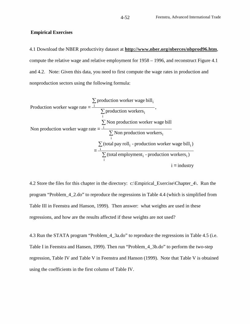
Feenstra, Advanced International Trade4-52
Empirical Exercises
4.1 Download the NBER productivity dataset at http://www.nber.org/nberces/nbprod96.htm,
compute the relative wage and relative employment for 1958 – 1996, and reconstruct Figure 4.1
and 4.2. Note: Given this data, you need to first compute the wage rates in production and
nonproduction sectors using the following formula:
industryi
)workersproduction-employment(total
)billgeworker waproduction-rollpay(total
workersproductionNon
billgeworker waproductionNonrategeworker waproductionNon
,workersproduction
billgeworker waproductionrategeworker waProduction
iii
iii
ii
i
ii
ii
=
=
=
=
∑
∑
∑
∑
∑
∑
4.2 Store the files for this chapter in the directory: c:\Empirical_Exercise\Chapter_4\. Run the
program “Problem_4_2.do” to reproduce the regressions in Table 4.4 (which is simplified from
Table III in Feenstra and Hanson, 1999). Then answer: what weights are used in these
regressions, and how are the results affected if these weights are not used?
4.3 Run the STATA program “Problem_4_3a.do” to reproduce the regressions in Table 4.5 (i.e.
Table I in Feenstra and Hansen, 1999). Then run “Problem_4_3b.do” to perform the two-step
regression, Table IV and Table V in Feenstra and Hanson (1999). Note that Table V is obtained
using the coefficients in the first column of Table IV.
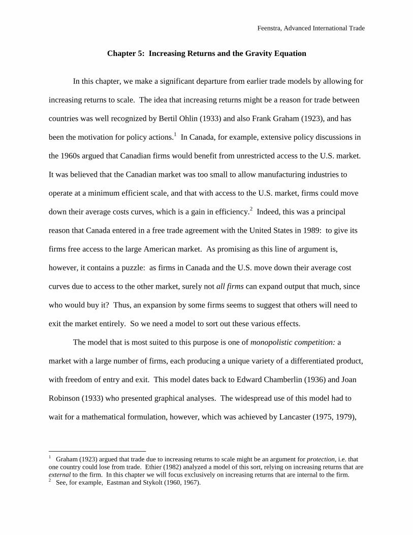
Feenstra, Advanced International Trade
Chapter 5: Increasing Returns and the Gravity Equation
In this chapter, we make a significant departure from earlier trade models by allowing for
increasing returns to scale. The idea that increasing returns might be a reason for trade between
countries was well recognized by Bertil Ohlin (1933) and also Frank Graham (1923), and has
been the motivation for policy actions.1 In Canada, for example, extensive policy discussions in
the 1960s argued that Canadian firms would benefit from unrestricted access to the U.S. market.
It was believed that the Canadian market was too small to allow manufacturing industries to
operate at a minimum efficient scale, and that with access to the U.S. market, firms could move
down their average costs curves, which is a gain in efficiency.2 Indeed, this was a principal
reason that Canada entered in a free trade agreement with the United States in 1989: to give its
firms free access to the large American market. As promising as this line of argument is,
however, it contains a puzzle: as firms in Canada and the U.S. move down their average cost
curves due to access to the other market, surely not all firms can expand output that much, since
who would buy it? Thus, an expansion by some firms seems to suggest that others will need to
exit the market entirely. So we need a model to sort out these various effects.
The model that is most suited to this purpose is one of monopolistic competition: a
market with a large number of firms, each producing a unique variety of a differentiated product,
with freedom of entry and exit. This model dates back to Edward Chamberlin (1936) and Joan
Robinson (1933) who presented graphical analyses. The widespread use of this model had to
wait for a mathematical formulation, however, which was achieved by Lancaster (1975, 1979),
1 Graham (1923) argued that trade due to increasing returns to scale might be an argument for protection, i.e. thatone country could lose from trade. Ethier (1982) analyzed a model of this sort, relying on increasing returns that areexternal to the firm. In this chapter we will focus exclusively on increasing returns that are internal to the firm.2 See, for example, Eastman and Stykolt (1960, 1967).
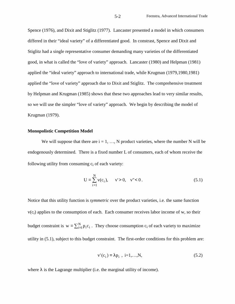
Feenstra, Advanced International Trade5-2
Spence (1976), and Dixit and Stiglitz (1977). Lancaster presented a model in which consumers
differed in their “ideal variety” of a differentiated good. In constrast, Spence and Dixit and
Stiglitz had a single representative consumer demanding many varieties of the differentiated
good, in what is called the “love of variety” approach. Lancaster (1980) and Helpman (1981)
applied the “ideal variety” approach to international trade, while Krugman (1979,1980,1981)
applied the “love of variety” approach due to Dixit and Stiglitz. The comprehensive treatment
by Helpman and Krugman (1985) shows that these two approaches lead to very similar results,
so we will use the simpler “love of variety” approach. We begin by describing the model of
Krugman (1979).
Monopolistic Competition Model
We will suppose that there are i = 1, …, N product varieties, where the number N will be
endogenously determined. There is a fixed number L of consumers, each of whom receive the
following utility from consuming ci of each variety:
0"v,0'v),c(vUN
1ii <>= ∑
=. (5.1)
Notice that this utility function is symmetric over the product varieties, i.e. the same function
v(ci) applies to the consumption of each. Each consumer receives labor income of w, so their
budget constraint is ∑ == N1i iicpw . They choose consumption ci of each variety to maximize
utility in (5.1), subject to this budget constraint. The first-order conditions for this problem are:
ii p)c('v λ= , i=1,…,N, (5.2)
where λ is the Lagrange multiplier (i.e. the marginal utility of income).
Feenstra, Advanced International Trade5-3
The effect of a change in price on consumption can be derived by totally differentiating
the system of equations in (5.2), together with the budget constraint. Normally, such a change in
price would affect λ. However, it can be argued that if the number of varieties is sufficiently
large, so that the budget share of each of them is small, then we can ignore the impact of a
change in one price on λ. In that case, the effect of a change in price is simply:
λ= ii dpdc"v 0"vdp
dc
i
i <λ=⇒ (5.3)
Using (5.2) and (5.3), we define the elasticity of demand for variety i as:
−=−=η
"vc
'v
c
p
dp
dc
iii
ii > 0. (5.4)
While the assumptions we have made on v (increasing and concave) ensure that the elasticity is
positive, we do not in general know whether it is increasing or decreasing in ci. This will turn
out to be quite important, and we shall assume that 0dc/d ii <η , so that as we move up a
demand curve (consumption falling) the elasticity rises. The reader should verify that this
assumption holds for a linear demand curve, and more generally, for any demand curve that is
“less convex” that a constant-elasticity curve.
On the production side, labor is the only resource and each firm requires the following
labor to produce output of yi:
ii yL β+α= , (5.5)
Feenstra, Advanced International Trade5-4
where α is the fixed labor input needed for production, and β is the marginal labor input. Given
the equilibrium wage w, it follows that average costs for the firms are, == iii y/wLAC
β+α wy/w i , while marginal costs are simply wβ. These are both graphed in Figure 5.1.
Monopolistic competition has two key equilibrium conditions for firms. First, each firm
maximizes its own profits, requiring that marginal revenue equal marginal cost (MR=MC).
Second, there is free entry whenever economic profits are positive, so in the long-run equilibrium
we must have zero profits, or price equal to average cost (P=AC). In addition to these, we will
add the requirement that the equilibrium is “symmetric,” meaning that prices and quantities are
identical across varieties. Dropping the subscript i, we therefore have the equilibrium
conditions:
MR=MC: β=
η
− w1
1p , or
−ηηβ=
1w
p(5.6)
P=AC: β+
α= wy
wp , or β+
α=
Lcw
p(5.7)
Notice that in (5.7), we have replaced supply of each good, y, by the demand for each
good, Lc. Equations (5.6) and (5.7) form two equations to solve for the two unknowns, (p/w)
and c. The first of these equations is graphed as the line PP in Figure 5.2. Our assumption that
0dc/d ii <η ensures that the PP curve is upward sloping. Turning to equation (5.7), this is
graphed as the downward sloping line ZZ in Figure 5.2, which is simply the firm’s average cost
curve. The intersection of these two curves determines the equilibrium values of (p/w) and c.
Then to determine the equilibrium number of product N, we make use of full-employment in the
economy, which is stated as:
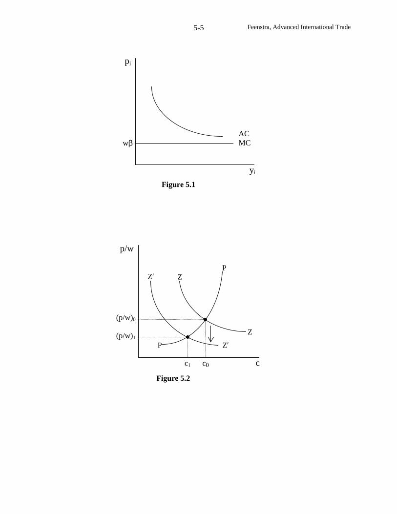
Feenstra, Advanced International Trade5-5
pi
wβ
yi
ACMC
Figure 5.1
Z′
Z′ Z
Z
P
P
p/w
(p/w)0
(p/w)1
c1 c0 c
Figure 5.2
Feenstra, Advanced International Trade5-6
)Lc(N)y(N)y(LLN
1ii
N
1ii β+α=β+α=β+α== ∑∑
==, (5.8)
from which it follows that:
]c)L/[(
1N
β+α= . (5.9)
The equilibrium value of c therefore determines the number of products N.
So far, we have represented the equilibrium for a single economy. But the effects of
trade are easily introduced. For example, suppose that two countries of identical size move from
autarky to free trade. Notice that because the economies are identical, then in the Heckscher-
Ohlin model there would be absolutely no reason for trade between them. But in the
monopolistic competition model, there will be a rationale for trade: firms will begin to export to
the other country, and at the same time, face competition from firms abroad. This increase in the
number of competitors can be expected to lower the equilibrium price. This is exactly what
happens, as can be confirmed from the equilibrium conditions.
Having the two identical countries trading is just like doubling the population L. This has
no impact on the PP curve [since L does not appear in (5.6)], but it does shift the ZZ curve down
[as can be seen from (5.7)]. Therefore, the equilibrium consumption of each variety falls, from
c0 to c1, while the real wage rises, from (w/p)0 to (w/p)1. Consumption falls because individuals
are spreading their expenditures over more product varieties, and this raises the elasticity of
demand, reducing the equilibrium prices and therefore raising real wages. This is a source of
gain for consumers. But there is also a second source of gain from trade, because with the rise in
L and fall in c, it can be verified from (5.9) that total product variety increases. That is, the sum
of varieties from both countries under free trade exceeds the number in any single country before
trade.
Feenstra, Advanced International Trade5-7
But notice that the number of varieties produced in each country necessarily falls with
the opening of trade. This can be seen by noting that the fall in (p/w), as firms move down their
average cost curve, necessarily implies that output y increases. This means that any firm that
produces both in autarky and under free trade will be selling more with trade. But the full-
employment conditions for each economy is )y(NL β+α= , where now L is fixed. So the
increase in y, as firms exploit economies of scale, necessarily implies a reduction in the number
of firms in each country. This resolves the question raised at the beginning of the chapter:
opening trade between countries indeed implies that firms must exit in each, while the remaining
firms expand their output and take advantage of scale economies.
Evidence from the Canada-U.S. Free Trade Agreement
To summarize, Krugman’s model contains two predictions concerning the impact of trade
on the productivity of firms: the scale effect, as surviving firms expand their outputs, and the
selection effect, as some firms are forced to exit. Which one of these effects is most important in
practice? This is a question of some importance since the dislocation of workers caused by the
bankruptcy of firms is bound to bring costs to them. This was certainly true in Canada after it
entered into the free trade agreement with the U.S. on January 1, 1989, because at the same time,
Canada also had a tight monetary policy that led to further job loss. The early computable
general equilibrium model of Harris (1984) and Cox and Harris (1985, 1986), done before the
1989 agreement, presumed substantial scale economies based on engineering estimates for
various industries, and predicted very high efficiency gains for Canada. These estimates were
influential in Canadian policy circles as the merits of the agreement with the U.S. were being
debated. With more than a decade since the Canada-U.S. FTA has been in effect, there are now
several studies we can look to that quantify the scale versus selection effect empirically.
Feenstra, Advanced International Trade5-8
The scale effect – that surviving firms will expand their scale of production following
trade liberalization – has unfortunately not been borne out empirically. Head and Ries (1999)
use plant level data for a sample of 230 Canadian industries over 1988-1994 to examine the
impact on plant scale in the six years following the free trade agreement with the United States.
They find that the tariff reductions in the U.S. increased plant scale in Canada by some 10% on
average, but this was largely offset by a 8.5% reduction in plant scale due to the reductions in
Canadian tariffs. On net, therefore, the free trade agreement had only a small impact on scale.
This type of evidence is also found from tariff reductions in a wide range of developing
countries, where the average scale of firms in import-competing industries either shrank
following liberalization, or expanded only slightly.3 The only silver lining to this result is that it
appears the extent of economies of scale is not that great in the first place, so that any reduction
in scale does not really cause higher costs. In addition, evidence from developing countries
shows that the markup of price over marginal costs is indeed reduced following tariff reductions,
so consumers gain in that respect.4
Turning to the selection effect, this is another avenue through which productivity in an
industry can change following liberalization. In particular, if the least-efficient firms are the ones
to exit, then average industry productivity will rise. Note that this is outside the framework of
the original Krugman model, since it makes the “symmetry” assumption that all firms were of
the same size and efficiency (it follows that the exit of some would not automatically change
average productivity). This assumption was made for analytical convenience, but contradicts the
empirical fact that every industry has a very wide range of firms operating within it. Indeed, it is
only recently that trade theory has caught up with this empirical fact, and there are now several
3 Tybout and Westbrook (1995) obtain this result for liberalization in Mexico during 1984-1990, whereas Tybout,de Melo and Corbo (1991) find evidence of small increases in scale following liberalization in Chile.
Feenstra, Advanced International Trade5-9
models that allows for a range of firms with differing productivities, due to Melitz (2002) and
Yeaple (2002), that can predict the effects of tariff reductions. In these models, the gains from
the Canada-U.S. free trade area would come not from scale effects, but rather, from selection
effects, whereby the least efficient firms exit after liberalization.
The empirical evidence on this comes from Trefler (2001), which is the first attempt to
comprehensively assess the impact of this agreement on productivity within Canada. Trefler
concludes that:
For industries subject to large tariff cuts (these are typically “low-end” manufacturing
industries), the short-run costs included a 15% decline in employment and about a 10%
decline in both output and the number of plants. Balanced against these large short-run
adjustment costs were long-run labour productivity gains of 17% or a spectacular 1.0%
per year. Although good capital stock and plant-level data are lacking, an attempt is made
to identify the sources of FTA-induced labour productivity growth. Surprisingly, this
growth is not due to rising output per plant, increased investment, or market share shifts
to high-productivity plants. Instead, half of the 17% labour productivity growth appears
due to favourable plant turnover (entry and exit) and rising technical efficiency.
Thus, productivity in Canada was increased due to free trade with the U.S. from the selection
effect, not the scale effect.
The finding that the scale of Canadian firms did not change much (on net) following the
FTA can be explained from several models, as discussed in Head and Ries (1999, 2002). We
note here one particularly simple theoretical result: if the elasticity of demand for product
varieties is constant, then firm scale will not change at all due to tariffs or trade liberalization. A
utility function that leads to this case is the constant elasticity of substitution (CES) function:
4 We will discuss the empirical link between tariffs and markups in chapter 10.
Feenstra, Advanced International Trade5-10
∑=
σ−σ=N
1i
/)1(i ,cU (5.10)
The elasticity of substitution between products is equal to σ > 1, which also equals the elasticity
of demand η when N is large. 5 This implies that the markup of prices over marginal costs is
fixed, p/(βw) = [σ/(σ-1)].
Substituting this optimal price into the expression for profits of the firm we obtain:
α−
−σβ=β+α
1
ywy)w(-py . (5.11)
In order to have zero profits in equilibrium, it follows that the output of firms is fixed at,
βα−σ= /)1(y . (5.12)
So there is no scale effect in a model using (5.10), though trade will still affect the product
variety available to consumers. The product variety produced in each country is readily solved
from (5.12) and the full-employment condition (5.8), obtaining ).y/(LN β+α= Thus, the
number of varieties produced does not change due to trade in this CES model, so there is no
selection effect either, but the number of varieties consumed will increase due to those available
from imports.6
The key advantage of using the CES functional form is that it is homothetic, whereas this
will not hold for any other choice of v(ci) in (5.1). For this reason the CES functional form is
commonly used in the monopolistic competition literature, and despite its special properties,
5 In problem 5.2 you are asked to derive the elasticity of demand and investigate other properties of the utilityfunction (10).6 If firms are heterogeneous, as in the model of Melitz (2002) and Yeaple (2001), then a selection effect will re-appear even using CES preferences.
Feenstra, Advanced International Trade5-11
and we shall also make use of it later in the chapter.7
The Gravity Equation
In the monopolistic competition model, each country will be exporting varieties of the
differentiated product to each other. While firms in different countries may produce the same
product varieties in autarky, we assume they can costlessly leave one variety and produce
another, so that with trade it is profit maximizing to produce different varieties. In other words,
the countries are completely specialized in different product varieties. Trade in these product
varieties is referred to as “intra-industry trade.” Notice that complete specialization and intra-
industry trade does not occur in the two-sector Heckscher-Ohlin model: countries may be
producing in the same industries, but they either export or import in each industry – not both. In
the Heckscher-Ohlin model with a continuum of goods, however, we do have complete
specialization in different products when factor prices are unequal, as described in chapter 3.
The common feature of the monopolistic competition model and the HO model with a continuum
of goods is that they both have many more goods than factors: that is what allows for complete
specialization in different product varieties across countries. In this case, it turns out that trade
patterns can be described by a remarkably simple equation called the “gravity equation.”
In its simplest form, the gravity equation states that the bilateral trade between two
countries is directly proportional to the product of the countries GDP’s. Thus, larger countries
will tend to trade more with each other, and countries that are more similar in their relative sizes
will also trade more. This equation performs extremely well empirically, as has been known
since the original work of Tinbergen (1962). Our goal in this section is to derive this simple
7 In problem 5.4, we provide an example of an indirect utility function that is still homothetic, but does not requireconstant price elasticities of demand.
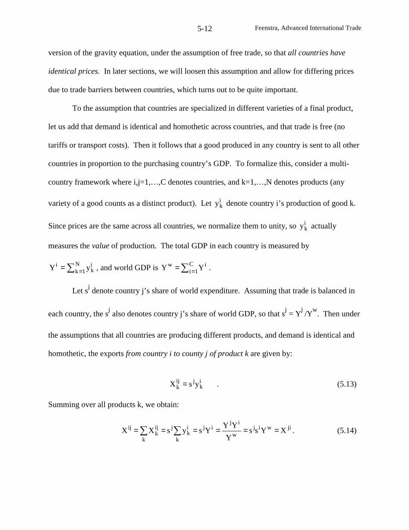
Feenstra, Advanced International Trade5-12
version of the gravity equation, under the assumption of free trade, so that all countries have
identical prices. In later sections, we will loosen this assumption and allow for differing prices
due to trade barriers between countries, which turns out to be quite important.
To the assumption that countries are specialized in different varieties of a final product,
let us add that demand is identical and homothetic across countries, and that trade is free (no
tariffs or transport costs). Then it follows that a good produced in any country is sent to all other
countries in proportion to the purchasing country’s GDP. To formalize this, consider a multi-
country framework where i,j=1,…,C denotes countries, and k=1,…,N denotes products (any
variety of a good counts as a distinct product). Let iky denote country i’s production of good k.
Since prices are the same across all countries, we normalize them to unity, so iky actually
measures the value of production. The total GDP in each country is measured by
∑ == N1k
ik
i yY , and world GDP is ∑ == C1i
iw YY .
Let sjdenote country j’s share of world expenditure. Assuming that trade is balanced in
each country, the sjalso denotes country j’s share of world GDP, so that s
j= Y
j/Y
w. Then under
the assumptions that all countries are producing different products, and demand is identical and
homothetic, the exports from country i to county j of product k are given by:
ik
jijk ysX = . (5.13)
Summing over all products k, we obtain:
jiwijw
ijij
k
ik
j
k
ijk
ij XYssY
YYYsysXX ====== ∑∑ . (5.14)
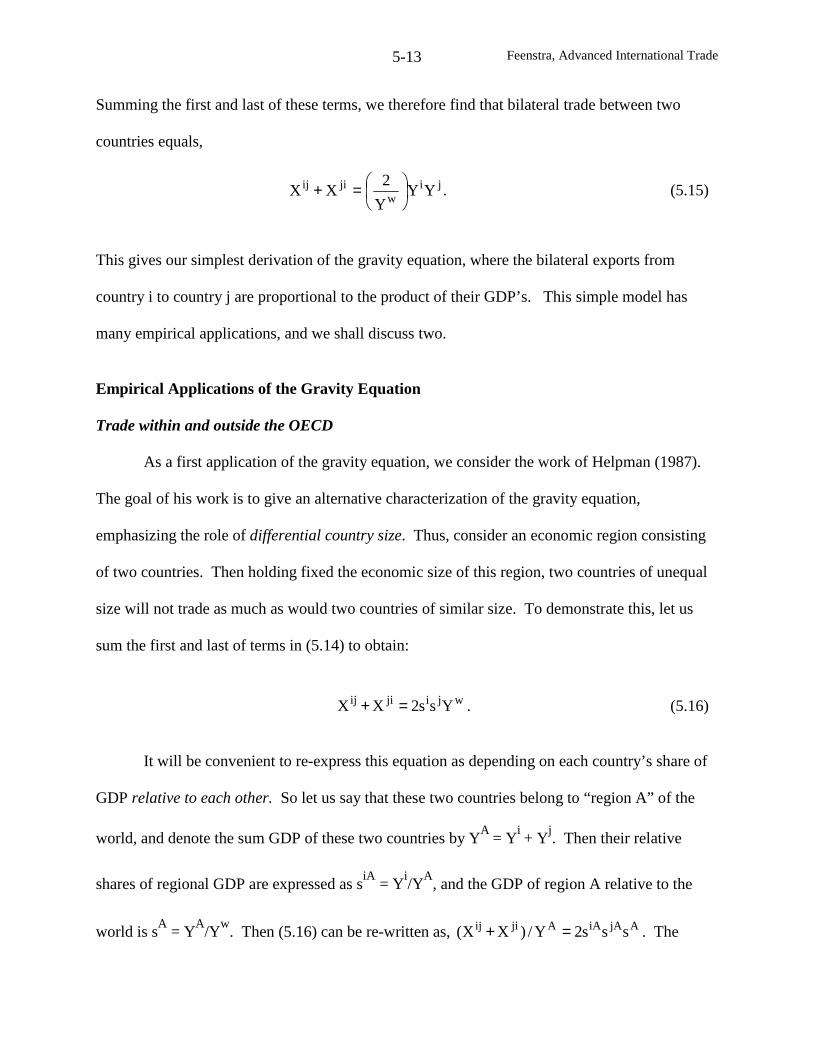
Feenstra, Advanced International Trade5-13
Summing the first and last of these terms, we therefore find that bilateral trade between two
countries equals,
jiw
jiij YYY
2XX
=+ . (5.15)
This gives our simplest derivation of the gravity equation, where the bilateral exports from
country i to country j are proportional to the product of their GDP’s. This simple model has
many empirical applications, and we shall discuss two.
Empirical Applications of the Gravity Equation
Trade within and outside the OECD
As a first application of the gravity equation, we consider the work of Helpman (1987).
The goal of his work is to give an alternative characterization of the gravity equation,
emphasizing the role of differential country size. Thus, consider an economic region consisting
of two countries. Then holding fixed the economic size of this region, two countries of unequal
size will not trade as much as would two countries of similar size. To demonstrate this, let us
sum the first and last of terms in (5.14) to obtain:
wjijiij Yss2XX =+ . (5.16)
It will be convenient to re-express this equation as depending on each country’s share of
GDP relative to each other. So let us say that these two countries belong to “region A” of the
world, and denote the sum GDP of these two countries by YA
= Yi+ Y
j. Then their relative
shares of regional GDP are expressed as siA
= Yi/Y
A, and the GDP of region A relative to the
world is sA
= YA
/Yw
. Then (5.16) can be re-written as, AjAiAAjiij sss2Y/)XX( =+ . The
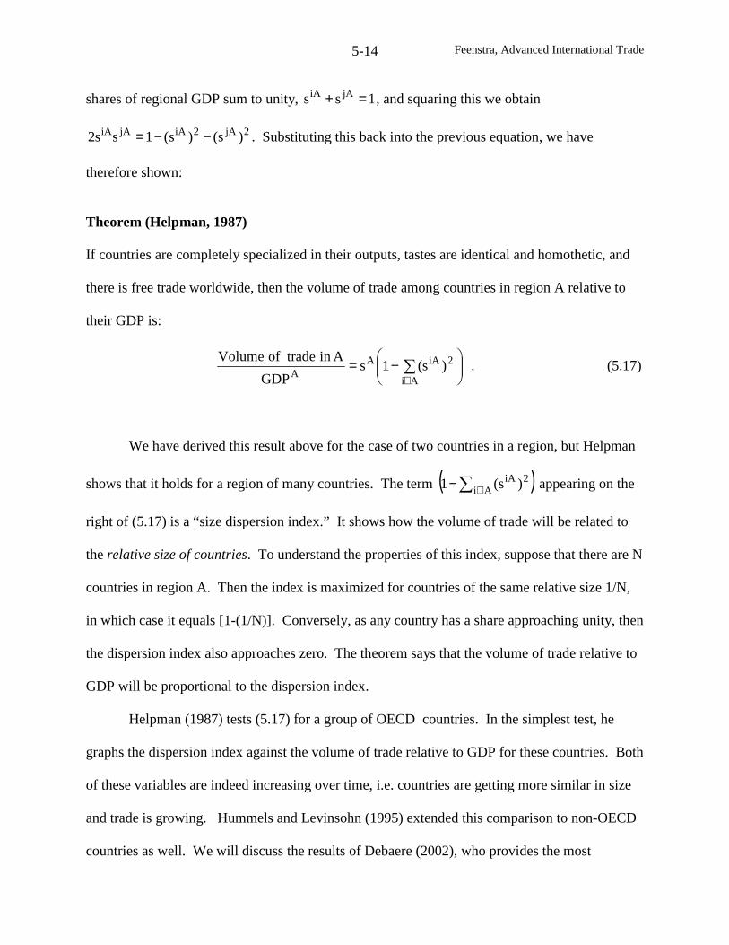
Feenstra, Advanced International Trade5-14
shares of regional GDP sum to unity, 1ss jAiA =+ , and squaring this we obtain
2jA2iAjAiA )s()s(1ss2 −−= . Substituting this back into the previous equation, we have
therefore shown:
Theorem (Helpman, 1987)
If countries are completely specialized in their outputs, tastes are identical and homothetic, and
there is free trade worldwide, then the volume of trade among countries in region A relative to
their GDP is:
−= ∑∈ Ai
2iAAA
)s(1sGDP
AintradeofVolume. (5.17)
We have derived this result above for the case of two countries in a region, but Helpman
shows that it holds for a region of many countries. The term ( )∑ ∈− Ai2iA )s(1 appearing on the
right of (5.17) is a “size dispersion index.” It shows how the volume of trade will be related to
the relative size of countries. To understand the properties of this index, suppose that there are N
countries in region A. Then the index is maximized for countries of the same relative size 1/N,
in which case it equals [1-(1/N)]. Conversely, as any country has a share approaching unity, then
the dispersion index also approaches zero. The theorem says that the volume of trade relative to
GDP will be proportional to the dispersion index.
Helpman (1987) tests (5.17) for a group of OECD countries. In the simplest test, he
graphs the dispersion index against the volume of trade relative to GDP for these countries. Both
of these variables are indeed increasing over time, i.e. countries are getting more similar in size
and trade is growing. Hummels and Levinsohn (1995) extended this comparison to non-OECD
countries as well. We will discuss the results of Debaere (2002), who provides the most
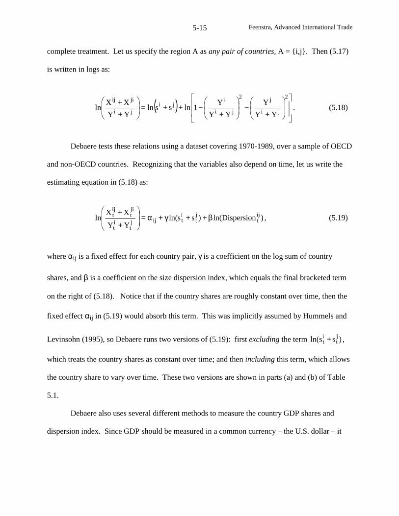
Feenstra, Advanced International Trade5-15
complete treatment. Let us specify the region A as any pair of countries, A = {i,j}. Then (5.17)
is written in logs as:
( )
+−
+−++=
++
2
ji
j2
ji
iji
ji
jiij
YY
Y
YY
Y1lnssln
YY
XXln . (5.18)
Debaere tests these relations using a dataset covering 1970-1989, over a sample of OECD
and non-OECD countries. Recognizing that the variables also depend on time, let us write the
estimating equation in (5.18) as:
)Dispersionln()ssln(YY
XXln ij
tjt
itijj
tit
jit
ijt β++γ+α=
+
+, (5.19)
where αij is a fixed effect for each country pair, γ is a coefficient on the log sum of country
shares, and β is a coefficient on the size dispersion index, which equals the final bracketed term
on the right of (5.18). Notice that if the country shares are roughly constant over time, then the
fixed effect αij in (5.19) would absorb this term. This was implicitly assumed by Hummels and
Levinsohn (1995), so Debaere runs two versions of (5.19): first excluding the term )ssln( jt
it + ,
which treats the country shares as constant over time; and then including this term, which allows
the country share to vary over time. These two versions are shown in parts (a) and (b) of Table
5.1.
Debaere also uses several different methods to measure the country GDP shares and
dispersion index. Since GDP should be measured in a common currency – the U.S. dollar – it
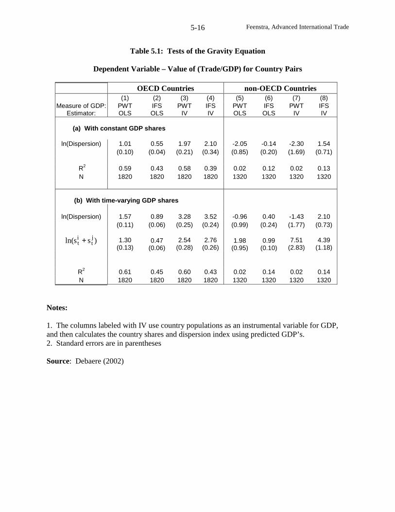
Feenstra, Advanced International Trade5-16
Table 5.1: Tests of the Gravity Equation
Dependent Variable – Value of (Trade/GDP) for Country Pairs
OECD Countries non-OECD Countries(1) (2) (3) (4) (5) (6) (7) (8)
Measure of GDP:Estimator:
PWTOLS
IFSOLS
PWTIV
IFSIV
PWTOLS
IFSOLS
PWTIV
IFSIV
(a) With constant GDP shares
ln(Dispersion) 1.01 0.55 1.97 2.10 -2.05 -0.14 -2.30 1.54(0.10) (0.04) (0.21) (0.34) (0.85) (0.20) (1.69) (0.71)
R2 0.59 0.43 0.58 0.39 0.02 0.12 0.02 0.13N 1820 1820 1820 1820 1320 1320 1320 1320
(b) With time-varying GDP shares
ln(Dispersion) 1.57 0.89 3.28 3.52 -0.96 0.40 -1.43 2.10(0.11) (0.06) (0.25) (0.24) (0.99) (0.24) (1.77) (0.73)
)ssln( jt
it + 1.30
(0.13)2.54
(0.28)2.76
(0.26)7.51
(2.83)4.39
(1.18)0.47
(0.06)1.98
(0.95)0.99
(0.10)
R2 0.61 0.45 0.60 0.43 0.02 0.14 0.02 0.14N 1820 1820 1820 1820 1320 1320 1320 1320
Notes:
1. The columns labeled with IV use country populations as an instrumental variable for GDP,and then calculates the country shares and dispersion index using predicted GDP’s.2. Standard errors are in parentheses
Source: Debaere (2002)

Feenstra, Advanced International Trade5-17
can be converted from national currencies using either nominal exchange rates or purchasing
power parity (PPP) exchange rates. The former – nominal GDP in U.S. dollars – is available
from the International Financial Statistics (IFS) of the International Monetary Fund, which is a
standard source for macroeconomic data across countries. The latter – real GDP converted to
dollars using PPP exchange rates – is available from the Penn World Tables (PWT). We would
expect that the latter is more reliable to construct the country GDP shares and dispersion index,
but report results from both PWT and IFS. In addition, Debaere reports results obtained when
country populations are used as an instrumental variable for GDP, so the country shares and
dispersion index are calculated using predicted GDP’s from this first-stage regression.
We are especially interested in testing whether β is close to unity, as Helpman’s equation
implies. The estimates of (5.19) over 14 OECD countries are shown in columns (1)-(4) of Table
5.1. Looking first at part (a) which ignores the term )ssln( jt
it + , in regression (1) using country
GDP’s from the PWT, we find that β is insignificantly different from unity. In regression (2),
using the GDP’s in nominal dollars from the IFS, β is estimated at 0.55 which is obviously less
than unity but is still positive and highly significant. The instrumental variable regressions in
columns (3) and (4) both have higher estimates of β on the dispersion index, but again they are
positive and highly significant. When the log sum of country shares is introduced in part (b), the
estimates of β are generally increased further.
For the group of non-OECD countries used, the results are quite different. Using real
GDP’s from the PWT, in columns (5) and (7), the dispersion index has a negative coefficient.
This contradicts Helpman’s results in (5.17), and more generally, contradicts the gravity
equation. We should not be surprised by this, however, because the gravity equation was based
on the assumption that countries are specialized in different goods. This may be a reasonable
Feenstra, Advanced International Trade5-18
description of trade between industrialized countries (e.g. Italian shoes are different from
American shoes), but it is a poor description of trade between developing countries that export
basic agricultural goods or low-skilled commodities. In that case, there is no reason at all for the
gravity equation to hold, and this is what we are finding in the non-OECD results where β is
negative.
It turns out that when nominal GDP’s from the IFS is used instead for the non-OECD
countries, as in columns (6) and (8), then β is instead positive but in most cases just barely
significant. In addition, the regressions for the non-OECD countries have much lower R2
than
for the OECD countries. In summary, the results in Table 5.1 show that Helpman’s formulation
of the gravity equation in (5.17) is strongly supported for the OECD countries, but receives little
or no support for the non-OECD countries. This accords with our expectation that specialization
in different goods is much more prevalent for the industrialized countries.
Trade within and between Canada and the U.S.
A second application of the gravity model, and one that has stimulated a large amount of
research, came from comparing intra-national trade between Canadian provinces to
international trade between Canadian provinces and U.S. states. This was the question posed by
McCallum (1995) in a study using 1988 data, just before the Canada-U.S. FTA was signed. He
estimated a gravity model like (5.15) where bilateral trade between Canadian provinces, or
between a Canadian province and U.S. state, should depend on each of their province or state
GDP’s. Specifically, the regression estimated by McCallum is:
ijijijj
2i
1jiij dlnYYln)XXln( ε+ρ+γδ+β+β+α=+ , (5.20)
Feenstra, Advanced International Trade5-19
where δijis an indicator variable that equals unity for trade between two Canadian provinces and
zero otherwise, and dij
is the distance between any two provinces or states. The results from
estimating (5.20) using 1988 data are shown in column (1) of Table 5.2. The same regression
using 1993 data is shown in column (2). Note that McCallum’s dataset included trade between
Canadian provinces, and provinces and states, but not trade between the U.S. states. This is
added in column (3) using 1993 data, in which case we also include an indicator variable that
equals one when trade is between two U.S. states and zero otherwise.
The results in columns (1)-(3) show coefficients on provincial or state GDP close to
unity, and strong negative relationship between distance and trade. This is no surprise. What is
unexpected is the very large coefficient on cross-provincial trade: ranging from 3.09 in column
(1) to 2.75 in column (3). Taking the exponents of these, we obtain the estimates on “Canada
trade” shown at the bottom of the table, indicating the cross-provincial trade is some 22 times
larger than cross-border trade in 1988, and 15.7 times larger in 1993. These numbers are
extraordinarily high! They are meant to capture any and all factors that might impede trade
between the U.S. and Canada, or what we might call “border effects.” It seems nearly
unbelievable, however, that these factors would lead to 16 or 22 times more internal trade in
Canada than external trade.
How is it that the Canada-U.S. border can apparently have an impact this large? The
answer from recent work of Anderson and van Wincoop (2001) is that border effects have an
asymmetric effect on countries of different size, and in particular, have a larger effect on small
countries. To understand their argument, we can run through a numerical example using
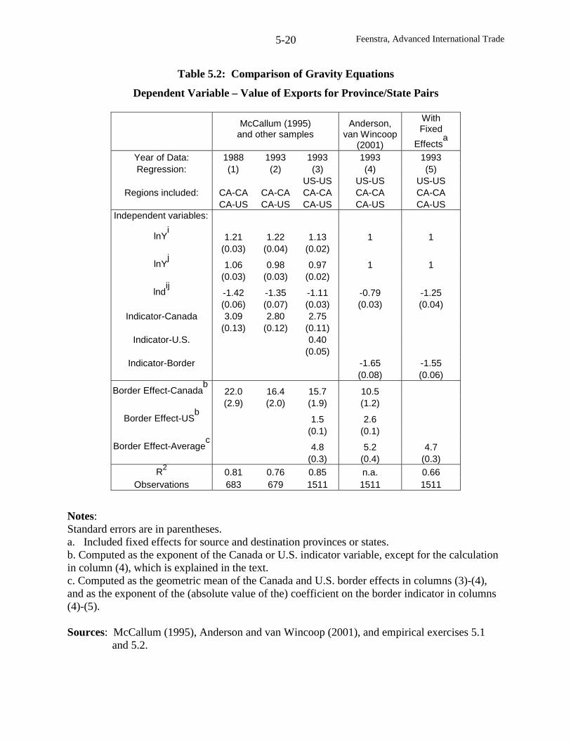
Feenstra, Advanced International Trade5-20
Table 5.2: Comparison of Gravity Equations
Dependent Variable – Value of Exports for Province/State Pairs
McCallum (1995)and other samples
Anderson,van Wincoop
(2001)
WithFixed
Effectsa
Year of Data: 1988 1993 1993 1993 1993Regression: (1) (2) (3) (4) (5)
US-US US-US US-USRegions included: CA-CA CA-CA CA-CA CA-CA CA-CA
CA-US CA-US CA-US CA-US CA-USIndependent variables:
lnYi
1.21 1.22 1.13 1 1(0.03) (0.04) (0.02)
lnYj
1.06 0.98 0.97 1 1(0.03) (0.03) (0.02)
lndij
-1.42 -1.35 -1.11 -0.79 -1.25(0.06) (0.07) (0.03) (0.03) (0.04)
Indicator-Canada 3.09 2.80 2.75(0.13) (0.12) (0.11)
Indicator-U.S. 0.40(0.05)
Indicator-Border -1.65 -1.55(0.08) (0.06)
Border Effect-Canadab
22.0 16.4 15.7 10.5(2.9) (2.0) (1.9) (1.2)
Border Effect-USb
1.5 2.6(0.1) (0.1)
Border Effect-Averagec
4.8 5.2 4.7(0.3) (0.4) (0.3)
R20.81 0.76 0.85 n.a. 0.66
Observations 683 679 1511 1511 1511
Notes:Standard errors are in parentheses.a. Included fixed effects for source and destination provinces or states.b. Computed as the exponent of the Canada or U.S. indicator variable, except for the calculationin column (4), which is explained in the text.c. Computed as the geometric mean of the Canada and U.S. border effects in columns (3)-(4),and as the exponent of the (absolute value of the) coefficient on the border indicator in columns(4)-(5).
Sources: McCallum (1995), Anderson and van Wincoop (2001), and empirical exercises 5.1and 5.2.
Feenstra, Advanced International Trade5-21
Canada-U.S. trade. Let us make the realistic assumption that the U.S. is 10 times bigger
economically. It follows that:
• With frictionless trade, Canada exports 90% of GDP to U.S., so it sells 10% internally
• Suppose the border effect reduces cross-border trade by a factor of one-half
• Then, Canada exports 45% of its GDP to U.S., so it must trade 55% internally
• So internal trade went up by 5.5 times (from 10% to 55%), cross-border down by one-
half (from 90% to 45%), and so internal trade has increased by 11 times more than cross-
border trade
• If we ask what has happened in the U.S., it used to export 10% of its output to Canada,
and now it exports only 5%. So internal trade has risen from 90% to 95% of output – a
modest change – while external trade has fallen in half. We conclude that cross-state
trade has increased by slightly more than 2 times cross-border trade.
We can see from this example that comparing cross-state trade to cross-border trade for
the U.S. (a large country) gives a reasonable estimate of the true border effect (which was a
factor of one-half), but that comparing cross-provincial trade with cross-border trade for Canada
(a small country) gives a really exaggerated estimate of the border effect. To avoid this bias, we
need to re-derive the gravity equation while introducing trade barriers (such as transport costs or
tariffs) right from the start. This means that prices differ across countries. Anderson (1979) was
the first to derive the gravity equation while taking into account these “price effects.” Estimating
the resulting equation still presents a challenge, however, and we shall discuss three approaches:
the use of prices indexes to measure the price effects in the gravity equation, as in Bergstrand
(1985,1989) and Baier and Bergstrand (2001); the use of estimated border effects to measure the
Feenstra, Advanced International Trade5-22
price effects, as in Anderson and van Wincoop (2001); and the use of fixed effects to account for
the price effects, as in Harrigan (1996), Hummels (1999), Redding and Venables (2000) and
others. Our derivation of the gravity equation follows Redding and Venables.
Border Effects in the Gravity Model
When there are border effects, such as transport costs or tariffs, then it is no longer the
case that prices are equalized across countries, so the pattern of trade is more complex than in the
gravity equation (5.15). The only way to sort this out is to assume a specific utility function, and
we shall adopt the CES specification. We let ijkc denote the exports from country i to country j
of good k. Because each country produces unique product varieties, the exports of good k from
country i to j are identical to the consumption of good k in country j. In contrast to Krugman’s
model, we now let ijkc denote total consumption of good k in country j, rather than per-capita
consumption. We will suppose that country i=1,…,C produces Ni
products. Then utility for
country j is:
∑ ∑= =
σ−σ=C
1i
N
1k
/)1(ijk
ji
,)c(U (5.21)
The triple-index on consumption is a bit unwieldy, but this can be simplified by assuming
that all products exported by country i sell for the same price pij
in country j. These prices are
inclusive of transport costs from country i to j, on a c.i.f. (cost, insurance, freight) basis. In
contrast, the local prices pifor goods produced in country i are net of any transport costs, on a
f.o.b. (free on board) basis. Let us model the relationship between these as: pij
= Tij
pi, where T
ii
= 1 and Tij
> 1, indicating that Tij
units of the product must be shipped to country j in order for
Feenstra, Advanced International Trade5-23
one unit to arrive; the amount (Tij
– 1) “melts” along the way. This formulation is called
“iceberg” transport costs and was introduced by Samuelson (1952).
With equal transport costs across varieties, then consumption in country j is also equal
over all the products k=1,…,Nisold by country i, so that ij
kc = ijc . Then the utility function is
simplified as:
∑=
σ−σ=C
1i
/)1(ijij )c(NU (5.22)
where cij
now denotes the consumption of any product sent from country i to country j.
The representative consumer in country j maximizes (5.22) subject to the budgetconstraint:
∑=
=C
1i
ijijij cpNY (5.23)
where Yjis aggregate expenditure and income in country j (we will assume balanced trade).
Maximizing (5.22) subject to (5.23), we can derive the following expression for the demand for
each product cij:8
)P/(Y)/Pp(c jj-jijij σ= , (5.24)
where Pjrefers to country j’s overall price index, defined as:
( ))(pNP )-11/(C1i
-1ijij σ=
σ∑= . (5.25)
8 See problem 5.2 to derive (5.24) and (5.25) when there are two goods.
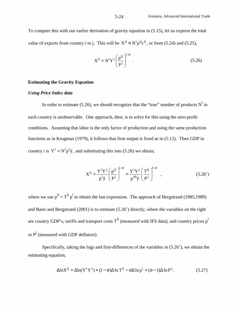
Feenstra, Advanced International Trade5-24
To compare this with our earlier derivation of gravity equation in (5.15), let us express the total
value of exports from country i to j. This will be ijijiij cpNX ≡ , or from (5.24) and (5.25),
P
pYNX
-1
j
ijjiij
σ
= . (5.26)
Estimating the Gravity Equation
Using Price Index data
In order to estimate (5.26), we should recognize that the “true” number of products Niin
each country is unobservable. One approach, then, is to solve for this using the zero-profit
conditions. Assuming that labor is the only factor of production and using the same production
functions as in Krugman (1979), it follows that firm output is fixed as in (5.12). Then GDP in
country i is ypNY iii = , and substituting this into (5.26) we obtain,
P
T
yp
YY
P
p
yp
YYX
-1
j
ij
i
ji-1
j
ij
i
jiij
σ
σ
σ
=
= , (5.26’)
where we use pij
= Tij
pito obtain the last expression. The approach of Bergstrand (1985,1989)
and Baier and Bergstrand (2001) is to estimate (5.26’) directly, where the variables on the right
are country GDP’s, tariffs and transport costs Tij
(measured with IFS data), and country prices pi
or Pj(measured with GDP deflators).
Specifically, taking the logs and first-differences of the variables in (5.26’), we obtain the
estimating equation,
jiijjiij Pln)1(plnTln)1()YYln(lnX ∆−σ+∆σ−∆σ−+∆=∆ . (5.27)
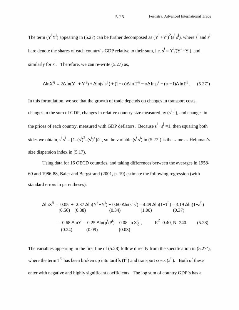
Feenstra, Advanced International Trade5-25
The term (YiY
j) appearing in (5.27) can be further decomposed as (Y
i+Y
j)2(s
isj), where s
iand s
j
here denote the shares of each country’s GDP relative to their sum, i.e. si= Y
i/(Y
i+Y
j), and
similarly for sj. Therefore, we can re-write (5.27) as,
jiijjijiij Pln)1(plnTln)1()ssln()YYln(2lnX ∆−σ+∆σ−∆σ−+∆++∆=∆ . (5.27’)
In this formulation, we see that the growth of trade depends on changes in transport costs,
changes in the sum of GDP, changes in relative country size measured by (sisj), and changes in
the prices of each country, measured with GDP deflators. Because si+s
j=1, then squaring both
sides we obtain, sisj= [1–(s
i)2–(s
j)2]/2 , so the variable (s
isj) in (5.27’) is the same as Helpman’s
size dispersion index in (5.17).
Using data for 16 OECD countries, and taking differences between the averages in 1958-
60 and 1986-88, Baier and Bergstrand (2001, p. 19) estimate the following regression (with
standard errors in parentheses):
∆lnXij
= 0.05 + 2.37 ∆ln(Yi+Y
j) + 0.60 ∆ln(s
isj) – 4.49 ∆ln(1+τij
) – 3.19 ∆ln(1+aij)
(0.56) (0.38) (0.34) (1.00) (0.37)
– 0.68 ∆lnYj– 0.25 ∆ln(p
i/P
j) – 0.08 ij
0Xln , R2=0.40, N=240. (5.28)
(0.24) (0.09) (0.03)
The variables appearing in the first line of (5.28) follow directly from the specification in (5.27’),
where the term Tij
has been broken up into tariffs (τij) and transport costs (a
ij). Both of these
enter with negative and highly significant coefficients. The log sum of country GDP’s has a
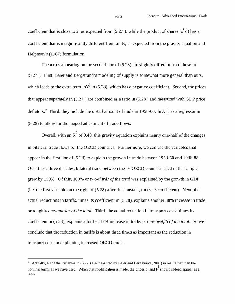
Feenstra, Advanced International Trade5-26
coefficient that is close to 2, as expected from (5.27’), while the product of shares (sisj) has a
coefficient that is insignificantly different from unity, as expected from the gravity equation and
Helpman’s (1987) formulation.
The terms appearing on the second line of (5.28) are slightly different from those in
(5.27’). First, Baier and Bergstrand’s modeling of supply is somewhat more general than ours,
which leads to the extra term lnYjin (5.28), which has a negative coefficient. Second, the prices
that appear separately in (5.27’) are combined as a ratio in (5.28), and measured with GDP price
deflators.9 Third, they include the initial amount of trade in 1958-60, ij0Xln , as a regressor in
(5.28) to allow for the lagged adjustment of trade flows.
Overall, with an R2
of 0.40, this gravity equation explains nearly one-half of the changes
in bilateral trade flows for the OECD countries. Furthermore, we can use the variables that
appear in the first line of (5.28) to explain the growth in trade between 1958-60 and 1986-88.
Over these three decades, bilateral trade between the 16 OECD countries used in the sample
grew by 150%. Of this, 100% or two-thirds of the total was explained by the growth in GDP
(i.e. the first variable on the right of (5.28) after the constant, times its coefficient). Next, the
actual reductions in tariffs, times its coefficient in (5.28), explains another 38% increase in trade,
or roughly one-quarter of the total. Third, the actual reduction in transport costs, times its
coefficient in (5.28), explains a further 12% increase in trade, or one-twelfth of the total. So we
conclude that the reduction in tariffs is about three times as important as the reduction in
transport costs in explaining increased OECD trade.
9 Actually, all of the variables in (5.27’) are measured by Baier and Bergstrand (2001) in real rather than the
nominal terms as we have used. When that modification is made, the prices pi
and Pj
should indeed appear as aratio.
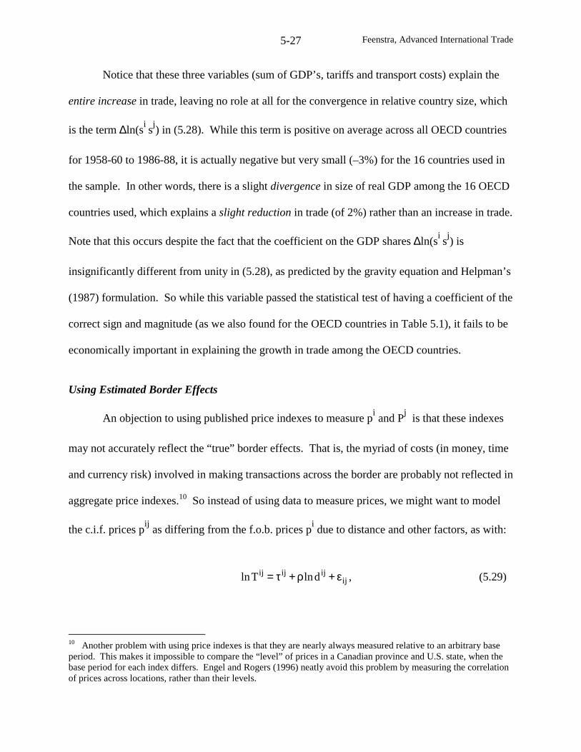
Feenstra, Advanced International Trade5-27
Notice that these three variables (sum of GDP’s, tariffs and transport costs) explain the
entire increase in trade, leaving no role at all for the convergence in relative country size, which
is the term ∆ln(sisj) in (5.28). While this term is positive on average across all OECD countries
for 1958-60 to 1986-88, it is actually negative but very small (–3%) for the 16 countries used in
the sample. In other words, there is a slight divergence in size of real GDP among the 16 OECD
countries used, which explains a slight reduction in trade (of 2%) rather than an increase in trade.
Note that this occurs despite the fact that the coefficient on the GDP shares ∆ln(sisj) is
insignificantly different from unity in (5.28), as predicted by the gravity equation and Helpman’s
(1987) formulation. So while this variable passed the statistical test of having a coefficient of the
correct sign and magnitude (as we also found for the OECD countries in Table 5.1), it fails to be
economically important in explaining the growth in trade among the OECD countries.
Using Estimated Border Effects
An objection to using published price indexes to measure piand P
jis that these indexes
may not accurately reflect the “true” border effects. That is, the myriad of costs (in money, time
and currency risk) involved in making transactions across the border are probably not reflected in
aggregate price indexes.10 So instead of using data to measure prices, we might want to model
the c.i.f. prices pij
as differing from the f.o.b. prices pidue to distance and other factors, as with:
ijijijij dlnTln ε+ρ+τ= , (5.29)
10 Another problem with using price indexes is that they are nearly always measured relative to an arbitrary baseperiod. This makes it impossible to compare the “level” of prices in a Canadian province and U.S. state, when thebase period for each index differs. Engel and Rogers (1996) neatly avoid this problem by measuring the correlationof prices across locations, rather than their levels.
Feenstra, Advanced International Trade5-28
where dij
is the distance between country i and j, τijis any other “border effect” associated with
selling from country i to j, and εij is a random error. We should think of ρ and τijas being
estimated, though we will have to explain how this is done. Generally, Tij
is meant to include all
effects limiting trade between countries i and j, so referring to it as “iceberg” transportation costs
is something of a misuse of language.
Substituting (5.29) back into the gravity equation (5.26) to eliminate the terms pij
= Tij
pi,
we obtain a set of equations where the exports between country i and j depend on the parameters
τijand ρ. This set of equations is highly non-linear, however, so it is difficult to estimate these
parameters directly. Instead, the approach of Anderson and van Wincoop (2001) is to further
simplify the gravity equation making use of the market clearing conditions, as follows.
Notice that with the iceberg transportation costs, the output of the firm exceeds the net
amount received by consumer, since these are related by:
ijC1j
iji Tcy ∑ == . (5.30)
Multiplying this by the price pi, we obtain ∑ == C
1jijijii cpyp , which is an equality between the
value of output of the firm (using the f.o.b. prices but before the output has “melted”) and the
expenditure of consumers (using the c.i.f. prices but after the quantity delivered has “melted”).
In principle, we can use the market clearing conditions (5.30) to solve for the unknown prices pi.
Rather than obtain an explicit solution for prices, Anderson and van Wincoop (2001) make use of
a convenient implicit solution. To develop their result, we again denote country i’s GDP by
iiii ypNY = , world GDP by ∑ == C1j
jw YY , and country i’s share by si= Y
i/Y
w.
Feenstra, Advanced International Trade5-29
Theorem (Anderson and van Wincoop, 2001)
Suppose that the transportation costs are symmetric, Tij
= Tji. Then an implicit solution to the
market clearing conditions (5.30) is:
( ) i)1/(1iii P~
/N/sp~σ−
≡ , (5.31)
in which case the price indexes are solved as:
σ1iC1i
iji-1j )P~
/(Ts)P~
( −=
σ ∑= . (5.32)
Proof:
We will show that substituting (5.31) into the price index (5.25), and substituting (5.31) into the
market clearing conditions (5.30), both lead to equation (5.32). First, substituting ijiij Tp~p~ =
( ) iij)1/(1ii P~
/TN/sσ−
= into (5.25), we immediately obtain (5.32). Second, rewrite the market
clearing conditions (5.30) as,
iiii ypNY = = ijC1j
ijii TcpN ∑ =ijC
1jiji pcN ∑ == j1jC
1jijii Y)P/Tp(N σ−
=∑= , (5.33)
where the final equality makes use of (5.24) and pij
= Tij
pi. Then substituting (5.31) into the
final expression of (5.33), we obtain,
j1jiC1j
ijii Y)P~
P~
/T(sY σ−=∑= . (5.34)
Summing this over i=1,…,C, we have, j1jiC1j
ijw Y)P~
P~
/T(Y σ−=∑= , which is identical to (5.32)
provided that Tij
= Tji. QED
Feenstra, Advanced International Trade5-30
To see the usefulness of this result, substitute (5.31) into the gravity equation (5.26) to
obtain:
σσ
=
=
-1
ji
ij
w
ji-1
ji
ijjiij
P~
P~T
Y
YY
P~
P~T
YsX . (5.35)
This is a remarkably simple equation, whereby bilateral trade between countries depends on their
GDP’s and also their implicit price indexes. Anderson and van Wincoop call iP~
“indexes of
multilateral resistance,” because they depend on the transport costs Tij
in (5.32). These indexes
are unobserved, but Anderson and van Wincoop argue that we can solve for them by using
equation (5.32) in combination with a formula for the transportation costs such as (5.29’).11
Specifically, the estimation strategy of Anderson and van Wincoop is to move the GDP
terms from the right to the left of (5.35), take logs and substitute (5.29) for the transportation
costs, obtaining (without the constant term Yw
):
ij1j1iijijjiij )1()P
~ln()P
~ln()1(dln)1()YY/ln(X εσ−+++τσ−+σ−ρ= −σ−σ . (5.36)
The dependent variable on the left is bilateral trade relative to the product of GDP’s. On the
right we have distance between regions i and j, followed by all other border effects (1–σ)τij, and
then the multilateral resistance terms 1i )P~
( −σ . These terms can be solved from (5.32)
11 Notice that (5.32) determines iP~ as a function of the transport costs Tij. We can write (5.32) alternatively as,
σ1)P
~P~
/C1i (Ts1
jiiji −∑ == , which shows that a weighted average of the terms σ−1)P~
P~
/(T jiij sums to unity, implying
that these terms themselves are centered around unity. When Tij = 1 for all i, j, for example, then the solution to
(5.32) is 1P~i = for all i. Note that in general the solution to (5.32) involves a normalization on the absolute level of
prices, and therefore, on the absolute level of the implicit price indexes.
Feenstra, Advanced International Trade5-31
once we know the transportation costs Tij
= Tji
. The transport costs, in turn, are obtained from
(5.29) using the estimated value of ijij )1(dln)1( τσ−+σ−ρ , which comes from (5.36). The
estimation of this system must be custom programmed to minimize the sum of squared residuals
in (5.36), while simultaneously using (5.29) to obtain the values of Tij
= Tji
at each iteration, and
with these, solving for the multilateral resistance terms 1i )P~
( −σ from (5.32).
To perform this estimation, we need to be more specific about the form of the border
effects (1-σ)τijin (5.36). Recall that in McCallum’s (1995) gravity equation in (5.20), we
introduced an indicator variable δijthat equaled unity for trade between two Canadian provinces,
and zero otherwise. Anderson and van Wincoop instead work with an indicator variable that is
(1–δij), or unity for trade between the U.S. and Canada, and zero otherwise. Introducing the
coefficient γ on this variable, we replace (1–σ)τijwith γ(1–δij
) in (5.36) and also use the
coefficient α = ρ(1–σ) on distance, to obtain:
ij1j1iijijjiij )1()P
~ln()P
~ln()1(dln)YY/ln(X εσ−+++δ−γ+α= −σ−σ . (5.37)
Their estimates of (5.37) are shown in column (4) of Table 5.2. Notice that the provincial
and states GDP terms have their coefficients constrained at unity, since they have been brought
to the left of (5.37). The coefficient on the indicator variable on cross-border trade in column (4)
is estimated at γ = –1.65. This can be compared to the estimates on the indicator variables for
intra-Canada trade and intra-U.S. trade, in column (3), of 2.75 and 0.40, respectively. We
certainly expect the indicator variables in columns (3) and (4) to have coefficients that are
opposite in sign, since in the one case we are measuring intranational trade and in the other case
Feenstra, Advanced International Trade5-32
measuring international trade. It is noteworthy, however, that Anderson and van Wincoop’s
estimate in column (4) is roughly midway between the conventional gravity estimates in column
(3), in absolute value. This appears to occur because Anderson and van Wincoop only allow a
single indicator variable to measure cross-border trade, rather than distinguishing two indicator
variables (i.e. one for Canadian exports to the U.S., and another for American exports to
Canada). The use of a single indicator variable is related to their assumption that transport costs
are symmetric, Tij
= Tji.
How should we interpret the estimate γ = –1.65? One approach is to recall that (1–σ)τij
was replaced by γ(1–δij) in (5.37), so setting these equal and taking the exponent, we solve for
exp(τij) = exp[γ(1–δij
)/(1–σ)]. For cross-border trade we have δij=0, so exp(τij
) = exp[γ/(1–σ)].
Taking values for the elasticity of substitution of σ = 5, 10 and 20, we would therefore obtain
estimates of exp(τij) of 1.5, 1.2, and 1.09, indicating border barriers of between 9% and 50% in
terms of their implied effect on price. The upper end of these estimates is certainly high, but the
lower end is not unreasonable.
We would like to turn the coefficient γ = –1.65 into an estimate of how much more trade
there is within Canada as compared to across the border. For regressions (1)-(3) in Table 5.2, we
simply took the exponent of the indicator coefficient, as reported near the bottom of the table.
That approach is no longer appropriate, however, because if the border did not exist then the
multilateral resistance terms in (5.37) would also be affected. Let us denote by 1i )P( −σ the
multilateral resistance terms in the absence of the border effect, i.e. what we obtain from formula
(5.32), but now using only distance (times its estimated coefficient) to compute Tij
in (5.29).
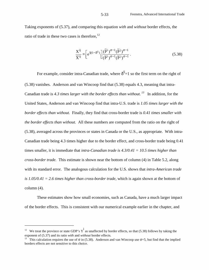
Feenstra, Advanced International Trade5-33
Taking exponents of (5.37), and comparing this equation with and without border effects, the
ratio of trade in these two cases is therefore,12
1j1i
1j1i)1(ˆ
ij
ij
)P()P(
)P~
()P~
(e
X
X ij
−σ−σ
−σ−σδ−γ
= . (5.38)
For example, consider intra-Canadian trade, where δij=1 so the first term on the right of
(5.38) vanishes. Anderson and van Wincoop find that (5.38) equals 4.3, meaning that intra-
Canadian trade is 4.3 times larger with the border effects than without. 13 In addition, for the
United States, Anderson and van Wincoop find that intra-U.S. trade is 1.05 times larger with the
border effects than without. Finally, they find that cross-border trade is 0.41 times smaller with
the border effects than without. All these numbers are computed from the ratio on the right of
(5.38), averaged across the provinces or states in Canada or the U.S., as appropriate. With intra-
Canadian trade being 4.3 times higher due to the border effect, and cross-border trade being 0.41
times smaller, it is immediate that intra-Canadian trade is 4.3/0.41 = 10.5 times higher than
cross-border trade. This estimate is shown near the bottom of column (4) in Table 5.2, along
with its standard error. The analogous calculation for the U.S. shows that intra-American trade
is 1.05/0.41 = 2.6 times higher than cross-border trade, which is again shown at the bottom of
column (4).
These estimates show how small economies, such as Canada, have a much larger impact
of the border effects. This is consistent with our numerical example earlier in the chapter, and
12 We treat the province or state GDP’s Yi
as unaffected by border effects, so that (5.38) follows by taking theexponent of (5.37) and its ratio with and without border effects.13 This calculation requires the use of σ in (5.38). Anderson and van Wincoop use σ=5, but find that the impliedborders effects are not sensitive to this choice.
Feenstra, Advanced International Trade5-34
indeed, the estimates of border effects obtained by Anderson and van Wincoop (10.5 and 2.6) are
nearly the same as in our simple numerical example. Furthermore, these estimates have the
following special property. The geometric mean of the border effects is (10.5⋅2.6)1/2
= 5.2.
Notice that this is the same as what we obtain by taking the exponent of the coefficient on the
cross-border indicator variable (in absolute value), 65.1e = 5.2. So the geometric mean of the
Canada and U.S. border effects, computing using formula (5.38), turns out to be identical to what
we obtain by just using the cross-border indicator variable! This is no coincidence, and we
provide a proof of this simple relation in the Appendix to this chapter. This result means that
using cross-border indicator variable is a completely valid way to infer the average impact of the
border on intranational relative to international trade.
Using Fixed Effects
A drawback to the estimation strategy of Anderson and van Wincoop is that it requires
custom programming to perform the constrained minimization (and obtain standard errors). A
third and final approach to estimating the gravity equation, while using ordinary least squares, is
to use fixed effects to take account of the unobserved price indexes. Fixed effects have been
used in the gravity equation by a number of authors, including Harrigan (1996) and Hummels
(1999), for example. Redding and Venables (2000) and Rose and van Wincoop (2001) give
these fixed effects a structural interpretation, and we will summarize each of their results.
Since the multilateral indexes in (5.37) are unobserved, rather than calculating them
according to (5.32), we could instead measure them as the coefficients of source and destination
region fixed effects. That is, let i1δ denote an indicator variable that is unity if region i is the
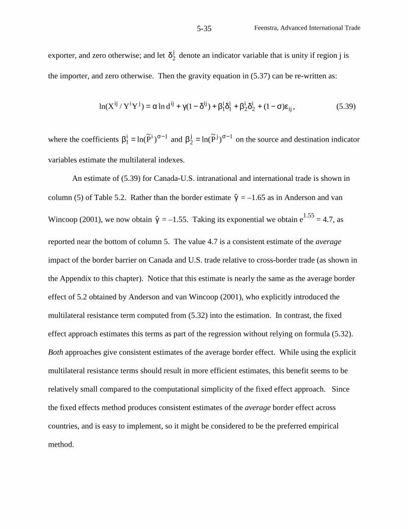
Feenstra, Advanced International Trade5-35
exporter, and zero otherwise; and let j2δ denote an indicator variable that is unity if region j is
the importer, and zero otherwise. Then the gravity equation in (5.37) can be re-written as:
iji2
i2
i1
i1
ijijjiij )1()1(dln)YY/ln(X εσ−+δβ+δβ+δ−γ+α= , (5.39)
where the coefficients 1ii1 )P
~ln( −σ=β and 1jj
2 )P~
ln( −σ=β on the source and destination indicator
variables estimate the multilateral indexes.
An estimate of (5.39) for Canada-U.S. intranational and international trade is shown in
column (5) of Table 5.2. Rather than the border estimate γ = –1.65 as in Anderson and van
Wincoop (2001), we now obtain γ = –1.55. Taking its exponential we obtain e1.55
= 4.7, as
reported near the bottom of column 5. The value 4.7 is a consistent estimate of the average
impact of the border barrier on Canada and U.S. trade relative to cross-border trade (as shown in
the Appendix to this chapter). Notice that this estimate is nearly the same as the average border
effect of 5.2 obtained by Anderson and van Wincoop (2001), who explicitly introduced the
multilateral resistance term computed from (5.32) into the estimation. In contrast, the fixed
effect approach estimates this terms as part of the regression without relying on formula (5.32).
Both approaches give consistent estimates of the average border effect. While using the explicit
multilateral resistance terms should result in more efficient estimates, this benefit seems to be
relatively small compared to the computational simplicity of the fixed effect approach. Since
the fixed effects method produces consistent estimates of the average border effect across
countries, and is easy to implement, so it might be considered to be the preferred empirical
method.
Feenstra, Advanced International Trade5-36
It is also interesting that the average border effect of 4.7 is nearly the same as the average
effect obtained by a conventional gravity equation (like McCallum, 1995): in column (3) of
Table 5.2, we compute the geometric mean of the border effect for Canada and the U.S. as 4.8.
In contrast to columns (4) and (5), the estimates in column (1)-(3) are not consistent, because
these regressions do not incorporate the price indexes. This appears to have the effect of
overstating the border effect for Canada [15.7 in column (3) as compared to 10.5 in column (4)],
and understating the effect for the United States [1.5 in column (3) as compared to 2.6 in column
(4)]. Still, for this dataset, the geometric mean of these inconsistent estimates gives an average
border effect that is very close to the consistent estimates in columns (4) and (5).
The fixed effect approach has been used by Rose and van Wincoop (2001) to estimate the
impact of monetary unions on international trade. They include an indicator variable that is unity
if the two countries belong to a monetary union, and interpret its coefficient of γ = 0.86 as a
consistent estimate of the average impact of monetary unions on trade. This interpretation is
valid (based on a multi-country extension of the Lemma in the Appendix). Surprisingly, they
find that monetary unions increase trade by γe = 2.36, or more than doubling trade on average
between union members relative to non-union members. The actual mechanism by which
monetary unions lead to such a large increase in trade remains quite unclear. Results like this
have led Obstfeld and Rogoff (2001) to identify large border effects from the gravity equations
as the cause of the “six major puzzles in international macroeconomics.”
The fixed effect method has also been used by Redding and Venables (2000) to
determine wages across countries. They do not rely on symmetric transportation costs, or the
above theorem of Anderson and van Wincoop, but instead work directly from the gravity
equation in (5.26). In their approach, the differentiated product is used as both consumer goods
Feenstra, Advanced International Trade5-37
and as intermediate inputs to production. Thus, proximity to trading partners affects a country’s
ability to export the differentiated good, and import the differentiated inputs: both of these
activities will impact wages. Redding and Venables show the fixed effects of the gravity
equation are directly related to equilibrium wages. In other words, the economic geography of a
country – measured by its distance from and access to trading partners – determines its wages
and hence its standard of living.
In the next section, we turn to another question of economic geography that has to do
with the location of firms. Specifically, as we consider regions or countries of differing size,
will the higher demand in large areas serve to attract more firms? Since each product is
produced by only one firm in our model, asking about the location of firms is the same as asking
about how many products Nieach country produces. We address this in the next section, using a
simplified framework where wages are constant and equal across countries.
The Home Market Effect
We will make the same assumptions on the differentiated good as in Krugman’s original
model: labor is the only input, and output yiof the typical firm in country i requires the labor
input Li= α + βy
i. In addition, we will suppose that there is a homogeneous good, and one unit
of that good requires one unit of labor. There are no transport costs in this good, so its price is
equalized across countries.14 Choosing the homogeneous good as the numeraire, and provided
that each country produces that good under trade, wages are therefore unity in all countries.
Having wages fixed will simplify our determination of Ni.
14 The assumption of zero transport costs on the numeraire good is important. Davis (1998) argues that we needhigher transport costs on the differentiated good than in the homogeneous product to obtain the home market effect,as derived below. See also Fujita, Krugman and Venables (1999, chapter 7).
Feenstra, Advanced International Trade5-38
On the demand side, we assume that a fixed share of income φ is spent on the
differentiated product, which provides utility given by the CES function in (5.21) or (5.22).15
Therefore, demand for each differentiated product is still given by (5.25), but replacing income
Yjby the amount φL
jactually spent on the differentiated product, we obtain:
jj-jijij P/L)P/p(c φ= σ . (5.40)
The output of firms is still given by (5.30), ijC1j
iji Tcy ∑ == . Because of the CES utility function,
this output will be fixed in a zero-profit equilibrium, βα−σ= /)1(y , as obtained in (5.12). So in
principle, the number of products in each country can be derived from the market clearing
conditions:
ijC1j
ijTcy ∑ == , i=1,…,C, (5.41)
where consumption depends on the price indexes Pjgiven by (5.25), which depend on the
number of products.
Rather than solving for the number of products in each country, we will instead solve for
the change in these as country size Ljvaries. The fact that the firm outputs are fixed on the left
of (5.41) implies that some combination of the consumptions in each country must also be fixed,
on the right. As a guess, let us suppose that consumption of every variety in each country is
fixed. Under our framework where wages are equalized across countries, the prices piand p
ijare
also fixed. Then we can totally differentiate (5.40) holding cij
fixed to obtain,
15 Denoting consumption of the homogeneous good by 0c , the utility function is: ( ) )1/(N1i
/)1(i
10 ccU
−σφσ=
σ−σφ− ∑= .
Feenstra, Advanced International Trade5-39
)1/(LPLP)1(0 jjjj −σ−=⇒+−σ= , (5.42)
where z/dzz = for any variable. Thus, price indexes in each country j will fall in direct
proportion to the rise in country GDP. Recall from (5.25) that the price indexes depend on the
number of product in each country. Thus, provided that there is a change in the number of
products consistent with jP in (5.42), then our initial assumption that the consumption cij
are
fixed is indeed correct.
To determine the change in the number of products, let us differentiate (5.25) to obtain,
( )N1
1P C
1iijij ∑ = φ
σ−= , (5.43)
where )Y/()cpN( jijijijij φ=φ denotes the share of products from country i in the differentiated
goods purchased by country j, with 1C
1iij =φ∑ = . Combining (5.42) and (5.43), we obtain an
extremely simple relationship between the change in GDP of each country and the change in the
number of products,
∑ = φ= C1i
ijij NL . (5.44)
We can use (5.44) to solve for the change in number of product iN provided that the matrix of
expenditure shares ][ ijφ=Φ is invertible. This will be true, for example, if each country
purchases a larger share of the differentiated product from itself than from other countries, so
that ijjj φ>φ for i≠j, as we shall assume.
When there are just two countries, we can express (5.44) in matrix notation as:
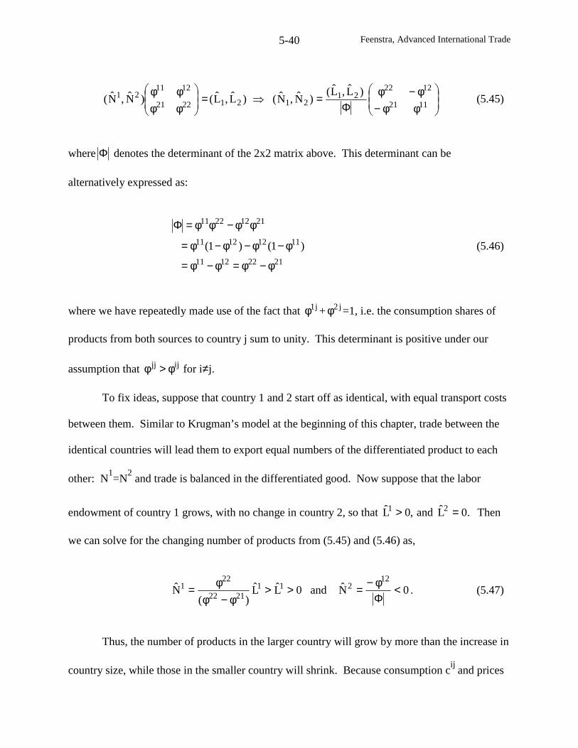
Feenstra, Advanced International Trade5-40
φφ−φ−φ
Φ=⇒=
φφφφ
1121
122221
21212221
121121 )L,L(
)N,N()L,L()N,N( (5.45)
where Φ denotes the determinant of the 2x2 matrix above. This determinant can be
alternatively expressed as:
21221211
11121211
21122211
)1()1(
φ−φ=φ−φ=
φ−φ−φ−φ=
φφ−φφ=Φ
(5.46)
where we have repeatedly made use of the fact that j1φ + j2φ =1, i.e. the consumption shares of
products from both sources to country j sum to unity. This determinant is positive under our
assumption that ijjj φ>φ for i≠j.
To fix ideas, suppose that country 1 and 2 start off as identical, with equal transport costs
between them. Similar to Krugman’s model at the beginning of this chapter, trade between the
identical countries will lead them to export equal numbers of the differentiated product to each
other: N1=N
2and trade is balanced in the differentiated good. Now suppose that the labor
endowment of country 1 grows, with no change in country 2, so that .0Land,0L 21 => Then
we can solve for the changing number of products from (5.45) and (5.46) as,
0Nand0LL)(
N12
2112122
221 <
Φφ−=>>
φ−φφ= . (5.47)
Thus, the number of products in the larger country will grow by more than the increase in
country size, while those in the smaller country will shrink. Because consumption cij
and prices
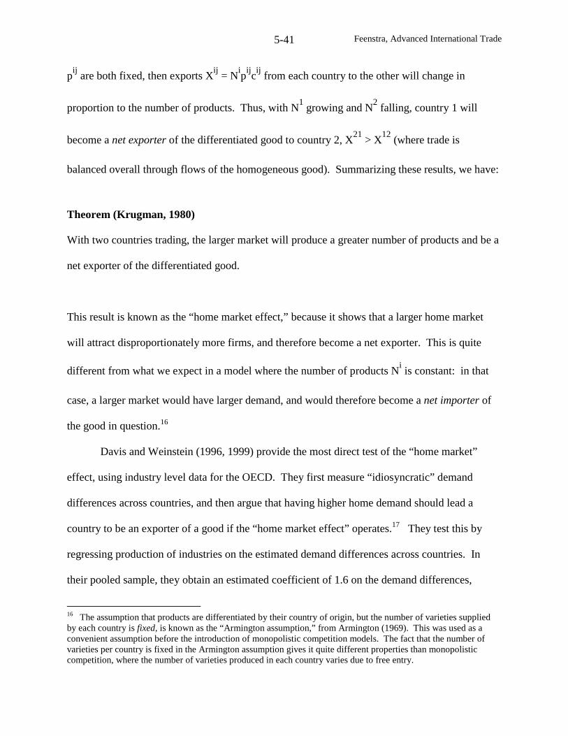
Feenstra, Advanced International Trade5-41
pij
are both fixed, then exports Xij
= Nip
ijc
ijfrom each country to the other will change in
proportion to the number of products. Thus, with N1
growing and N2
falling, country 1 will
become a net exporter of the differentiated good to country 2, X21
> X12
(where trade is
balanced overall through flows of the homogeneous good). Summarizing these results, we have:
Theorem (Krugman, 1980)
With two countries trading, the larger market will produce a greater number of products and be a
net exporter of the differentiated good.
This result is known as the “home market effect,” because it shows that a larger home market
will attract disproportionately more firms, and therefore become a net exporter. This is quite
different from what we expect in a model where the number of products Niis constant: in that
case, a larger market would have larger demand, and would therefore become a net importer of
the good in question.16
Davis and Weinstein (1996, 1999) provide the most direct test of the “home market”
effect, using industry level data for the OECD. They first measure “idiosyncratic” demand
differences across countries, and then argue that having higher home demand should lead a
country to be an exporter of a good if the “home market effect” operates.17 They test this by
regressing production of industries on the estimated demand differences across countries. In
their pooled sample, they obtain an estimated coefficient of 1.6 on the demand differences,
16 The assumption that products are differentiated by their country of origin, but the number of varieties suppliedby each country is fixed, is known as the “Armington assumption,” from Armington (1969). This was used as aconvenient assumption before the introduction of monopolistic competition models. The fact that the number ofvarieties per country is fixed in the Armington assumption gives it quite different properties than monopolisticcompetition, where the number of varieties produced in each country varies due to free entry.
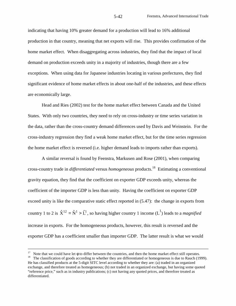
Feenstra, Advanced International Trade5-42
indicating that having 10% greater demand for a production will lead to 16% additional
production in that country, meaning that net exports will rise. This provides confirmation of the
home market effect. When disaggregating across industries, they find that the impact of local
demand on production exceeds unity in a majority of industries, though there are a few
exceptions. When using data for Japanese industries locating in various prefectures, they find
significant evidence of home market effects in about one-half of the industries, and these effects
are economically large.
Head and Ries (2002) test for the home market effect between Canada and the United
States. With only two countries, they need to rely on cross-industry or time series variation in
the data, rather than the cross-country demand differences used by Davis and Weinstein. For the
cross-industry regression they find a weak home market effect, but for the time series regression
the home market effect is reversed (i.e. higher demand leads to imports rather than exports).
A similar reversal is found by Feenstra, Markusen and Rose (2001), when comparing
cross-country trade in differentiated versus homogeneous products.18 Estimating a conventional
gravity equation, they find that the coefficient on exporter GDP exceeds unity, whereas the
coefficient of the importer GDP is less than unity. Having the coefficient on exporter GDP
exceed unity is like the comparative static effect reported in (5.47): the change in exports from
country 1 to 2 is 1112 LNX >= , so having higher country 1 income (L1) leads to a magnified
increase in exports. For the homogeneous products, however, this result is reversed and the
exporter GDP has a coefficient smaller than importer GDP. The latter result is what we would
17 Note that we could have let φ to differ between the countries, and then the home market effect still operates.18 The classification of goods according to whether they are differentiated or homogeneous is due to Rauch (1999).He has classified products at the 5-digit SITC level according to whether they are: (a) traded in an organizedexchange, and therefore treated as homogeneous; (b) not traded in an organized exchange, but having some quoted“reference price,” such as in industry publications; (c) not having any quoted prices, and therefore treated asdifferentiated.

Feenstra, Advanced International Trade5-43
expect from a model where the number of products in each country is fixed, so that higher
demand leads to net imports rather than net exports.
Conclusions
This chapter has covered material in two topics – trade under monopolistic competition
and the gravity equation – that are often linked though they need not be. As we have mentioned,
the gravity equation arises quite naturally whenever countries are specialized in different goods.
Such specialization is sometimes called “national product differentiation,” and cross-border trade
in different varieties of a good is referred to as “intra-industry trade.” This occurs under the
monopolistic competition model, but also occurs in other contexts, e.g. Dornbusch, Fischer, and
Samuelson’s (1977) Ricardian model with a continuum of goods, or their (1980) Heckscher-
Ohlin (HO) model where factor price are not equalized, as studied in chapter 3. Davis (1995)
has combined Ricardian and HO elements to generate intra-industry trade in a model where
product varieties have identical capital/labor ratios, but differ across countries by a Hicks-neutral
productivity term.19
So while complete specialization in goods can arise in a number of contexts, the CES
monopolistic competition model proves to be a convenient way to derive the gravity equation,
especially when we allow for transport costs and other trade barriers. Unlike early work on the
gravity equation that assumed identical prices across countries, once we introduce transportation
costs or any other border barriers then prices must differ internationally, so we need to take
account of the overall price indexes in each country. We have reviewed three methods to do so:
19 An elegant extension of Ricardian differences is provided by Eaton and Kortum (2001), who consider stochasticdifferences in the technologies across countries, with the lowest cost country becoming the exporter of each productvariety. They obtain a gravity-like equation, which should include country fixed effects that are related to theprobability distribution of technologies within each country.
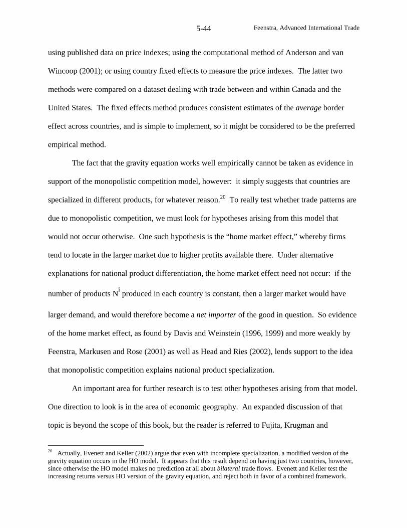
Feenstra, Advanced International Trade5-44
using published data on price indexes; using the computational method of Anderson and van
Wincoop (2001); or using country fixed effects to measure the price indexes. The latter two
methods were compared on a dataset dealing with trade between and within Canada and the
United States. The fixed effects method produces consistent estimates of the average border
effect across countries, and is simple to implement, so it might be considered to be the preferred
empirical method.
The fact that the gravity equation works well empirically cannot be taken as evidence in
support of the monopolistic competition model, however: it simply suggests that countries are
specialized in different products, for whatever reason.20 To really test whether trade patterns are
due to monopolistic competition, we must look for hypotheses arising from this model that
would not occur otherwise. One such hypothesis is the “home market effect,” whereby firms
tend to locate in the larger market due to higher profits available there. Under alternative
explanations for national product differentiation, the home market effect need not occur: if the
number of products Niproduced in each country is constant, then a larger market would have
larger demand, and would therefore become a net importer of the good in question. So evidence
of the home market effect, as found by Davis and Weinstein (1996, 1999) and more weakly by
Feenstra, Markusen and Rose (2001) as well as Head and Ries (2002), lends support to the idea
that monopolistic competition explains national product specialization.
An important area for further research is to test other hypotheses arising from that model.
One direction to look is in the area of economic geography. An expanded discussion of that
topic is beyond the scope of this book, but the reader is referred to Fujita, Krugman and
20 Actually, Evenett and Keller (2002) argue that even with incomplete specialization, a modified version of thegravity equation occurs in the HO model. It appears that this result depend on having just two countries, however,since otherwise the HO model makes no prediction at all about bilateral trade flows. Evenett and Keller test theincreasing returns versus HO version of the gravity equation, and reject both in favor of a combined framework.
Feenstra, Advanced International Trade5-45
Venables (1999), who describe many results building on increasing returns to scale and the
monopolistic competition model. For example, this literature suggests that proximity to markets
will raise wages, and Redding and Venables (2000) apply this idea to estimate wages across
countries based on the gravity equation. A similar approach can be used to determine wages
across cities or regions within a country, as in Hanson (1997, 1998).21 In other empirical work,
Davis and Weinstein (2001b) have used the location of economic activity in Japan, going from
prehistoric times to war-time dislocations to the present day, to evaluate the importance of
increasing returns versus alternative explanations for industry location.
Another direction to look for hypotheses is to loosen some of the assumptions of the
monopolistic competition model. Two key assumptions are that firms are symmetric (their costs
are all the same) and that they each produce a single product. Both of these assumptions are
patently false: every industry has a wide range of firms of various efficiencies, and many of
them produce multiple products. The theoretical difficulty with allowing for firms with differing
efficiency is that the zero-profit condition of monopolistic competition will no longer apply: if
the less-efficient firms earn zero profits, then the more-efficient firms will not. This difficulty
has been resolved in different ways by Melitz (2002) and Yeaple (2002). In Melitz’s model,
firms have random productivities and earn zero expected profits, while in Yeaple’s model, the
workers in more efficient firms receive higher wages, so profits are still zero. Both of these
models suggest empirical applications.
The assumption that firms in the monopolistic competition model each produce a single
product has be weakened by Feenstra, Huang and Hamilton (2003). They motivate the idea of
multi-product companies by the “business groups” that are found in many countries, such as the
21 See also the survey by Overman, Redding and Venables (2003). A theoretical model linking outsourcing andwages in an economic geography framework is provided by Gao (2002).
Feenstra, Advanced International Trade5-46
keiretsu in Japan and the chaebol in South Korea. In their model, a business group chooses its
range of upstream and downstream products to maximize profits, while free entry of groups
ensures that profits are zero in equilibrium. They show that that having multi-product groups has
a sharp implication for trade patterns: economies dominated by business groups will produce
less product variety than with single-product firms.22 This hypothesis can be tested by
comparing two economies of similar size but with differing structure of business groups. For
that purpose, Feenstra, Yang and Hamilton (1999) compare South Korea and Taiwan, where
Korea has the large and strongly integrated chaebol, whereas Taiwan has much smaller business
groups that are mainly located upstream. By comparing their sales of disaggregate products to
the United States, it is strongly confirmed that Taiwan sells a greater product variety to the U.S.
in nearly all industries than does Korea. Differences in the export patterns from South Korea and
Taiwan are also observed by Martins (1992) and Rodrik (1993), who attribute this to the group
structure in the two countries. Thus, the influence of business groups on the structure of trade, as
predicted by a monopolistic competition with multi-product companies, is supported by this
empirical evidence.
22 In addition, it turns out that there are multiple equilibria in the structure of business groups: an economy canhave a small number of large business groups, charging high prices for intermediates sold to other groups; or alarger number of smaller groups, charging lower prices for the sale of intermediates. Therefore, historical conditionsmust be considered to determine which equilibrium occurs in a country. Feenstra and Hamilton (2004) describe indetail the conditions that led Korea to an equilibrium with large business groups, and Taiwan to an equilibrium withsmaller groups.
Feenstra, Advanced International Trade5-47
Appendix: Using the Gravity Model to Measure Border Effects
The estimates of 10.5 for Canada and 2.6 for the U.S., shown in column (4) of Table 5.2,
are Anderson and van Wincoop’s (2001) “best” estimates of the impact of the Canada-U.S.
border on intra-Canadian and intra-American trade relative to cross-border trade. These are
unbiased estimates of the Canada-U.S. border effect, as opposed to the other estimates reported
near the bottom of columns (1)-(3), which are biased because the price terms are omitted from
the gravity equation. While the estimates of 10.5 and 2.6 require a complex calculation from
(5.38), the geometric mean of these two values can be obtained very simply from the gravity
equation, as indicated by the following result:
Lemma
Let γ denote the estimated coefficient of the border indicator in the gravity equation, and use
(5.38) to compute the impact of the border on intranational trade relative to international trade,
for each country. Then the geometric mean of the impact on each country equals γ−ˆe .
Proof:
The multilateral resistance terms in (5.38) are obtained from (5.32) using the transportation costs
Tij
= )1(ˆˆij ije)d( δ−γα (i.e. including border effects) to compute 1i )P
~( −σ , while using T
ij= αij )d(
(i.e. just distance) to compute 1i )P( −σ . Taking the geometric mean of trade Xij
between
Canadian provinces with border effects, and the predicted value ijX without border effects, we
obtain from (5.38):
N/1
CAj,i1j1i
1j1iN/1
CAj,iij
ij
)P()P(
)P~
()P~
(
X
X ∏∏∈
−σ−σ
−σ−σ
∈
=
. (5.48)
Feenstra, Advanced International Trade5-48
With CA={1,….,10} Canadian provinces, they can each sell to 9 others, making N= 90 bilateral
flows in (5.38a). (Notice that we exclude i=j from the calculations in (5.48), since we are not
considering sales by a province to itself.) In each of the bilateral flows, two indexes appear on
the right, so there are a total of 180 multilateral indexes in the numerator and in the denominator
of (5.48). Since each of the 10 provinces appears on the right of (5.48) an equal number of
times, i.e. 180/10 = 18 times, this expression can be simplified as,
5/1
CAi1i
1iN/1
CAj,iij
ij
)P(
)P~
(
X
X ∏∏∈
−σ
−σ
∈
=
, (5.48’)
where the exponent on the right is obtained as 18/90 = 1/5.
Using the same approach for the U.S.={1,…,30} American states in the sample, we can
compute that average trade between them with and without border effects as,
N/1
USj,i1j1i
1j1iN/1
USj,iij
ij
)P()P(
)P~
()P~
(
X
X ∏∏∈
−σ−σ
−σ−σ
∈
=
. (5.49)
where now N = 30⋅29 = 860. Again, for each bilateral flow there are two multilateral indexes in
the numerator and denominator on the right, so each of these indexes appears 860⋅2 = 1,720
times. Since each of the 30 states appears on the right of (5.49) an equal number of times, i.e.
1720/30 = 58 times, this expression can be simplified as,
15/1
USi1i
1iN/1
USj,iij
ij
)P(
)P~
(
X
X ∏∏∈
−σ
−σ
∈
=
, (5.49’)
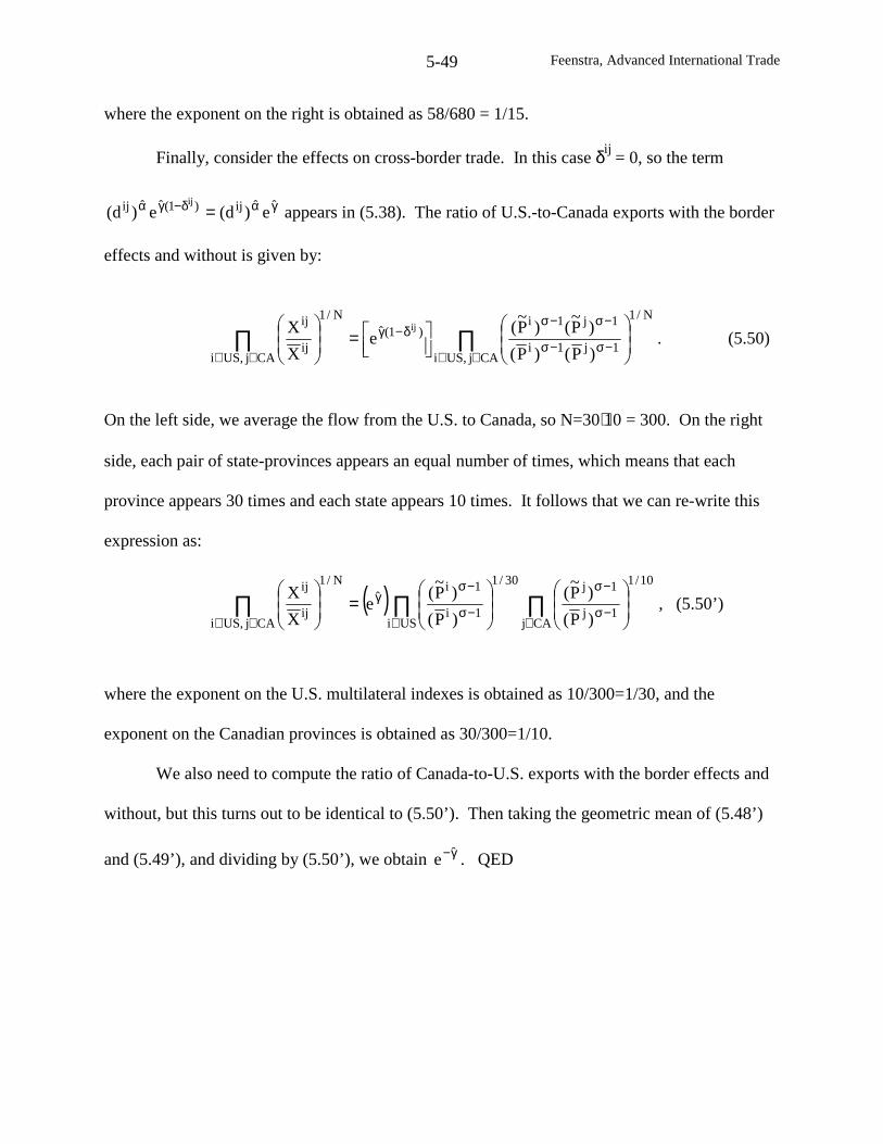
Feenstra, Advanced International Trade5-49
where the exponent on the right is obtained as 58/680 = 1/15.
Finally, consider the effects on cross-border trade. In this case δij= 0, so the term
γαδ−γα = ˆˆij)1(ˆˆij e)d(e)d(ij
appears in (5.38). The ratio of U.S.-to-Canada exports with the border
effects and without is given by:
∏∏∈∈
−σ−σ
−σ−σδ−γ
∈∈
=
CAj,USi
N/1
1j1i
1j1i)1(ˆ
CAj,USi
N/1
ij
ij
)P()P(
)P~
()P~
(e
X
X ij. (5.50)
On the left side, we average the flow from the U.S. to Canada, so N=30⋅10 = 300. On the right
side, each pair of state-provinces appears an equal number of times, which means that each
province appears 30 times and each state appears 10 times. It follows that we can re-write this
expression as:
( ) ∏∏∏∈
−σ
−σ
∈−σ
−σγ
∈∈
=
CAj
10/1
1j
1j
USi
30/1
1i
1iˆ
CAj,USi
N/1
ij
ij
)P(
)P~
(
)P(
)P~
(e
X
X, (5.50’)
where the exponent on the U.S. multilateral indexes is obtained as 10/300=1/30, and the
exponent on the Canadian provinces is obtained as 30/300=1/10.
We also need to compute the ratio of Canada-to-U.S. exports with the border effects and
without, but this turns out to be identical to (5.50’). Then taking the geometric mean of (5.48’)
and (5.49’), and dividing by (5.50’), we obtain γ−ˆe . QED
Feenstra, Advanced International Trade5-50
Problems
5.1 For the utility function in (5.1), with v(0) = 0, v’ > 0, and v” < 0, show that when the number
of goods rises holding income fixed, the consumer is better off.
5.2 In Krugman’s monopolistic competition model, suppose that the utility function takes on the
CES form shown in (5.10), rewritten for simplicity with two goods as:
.1/)1(0,cc)c,c(U 2121 <σ−σ=θ<+= θθ
Maximize this subject to the budget constraint, Icpcp 2211 ≤+ .
(a) Obtain an expression for the relative demand c1/c2 as a function of prices.
(b) The elasticity of substitution is defined as )p/pln(d/)c/cln(d 1221 . What is the value of the
elasticity of substitution for this utility function?
(c) Obtain an expression for the demands c1 and c2 as a function of prices.
(d) What do these expressions imply about the elasticity of demand?
5.3 Suppose that industry 1 is monopolistically competitive, with a CES sub-utility function as
described in problem 5.2. We let the marginal costs be denoted by c1(w,r), and the fixed costs in
the industry by αc1(w,r). That is, the fixed costs use labor and capital in the same proportions as
the marginal costs. Industry 2 is a competitive industry, and each industry uses labor and capital.
(a) Write down the relationship between the prices of goods and factor prices. Does the Stolper-
Samuelson Theorem still apply?
(b) Write down the full-employment conditions for the two factors. Does the Rybczynski
Theorem still apply in some form?
Feenstra, Advanced International Trade5-51
How are your answers to (a) and (b) affected if the fixed costs in industry 1 uses different
proportions of labor and capital than the marginal costs?
5.4 Consider the translog expenditure function:
ji
N
1i
N
1i
N
1jij2
1ii0 plnplnbplnaaUln)U,p(Eln ∑ ∑∑
= = =+++= , (5.51)
where:
,jiforN/band,N/)1N(b,N/1a ijiii ≠γ=−γ−== with i, j = 1,…,N, (5.52)
where γ > 0. Use this expenditure function to answer:
(a) Show that restrictions in (5.52) ensure that the expenditure function in (5.51) is
homogeneous of degree one in prices;
(b) Derive the share of expenditure on good i by differentiating (5.51) with respect to ln pi;
(c) Differentiate the share of each good with respect to ln pi to derive an expression for the
elasticity of demand;
(d) Use the elasticity of demand to obtain an expression for the ratio of price to marginal
cost for the firm. How will each firm’s price depend on its competitor’s prices?
Note that this expenditure function has been used by Bergin and Feenstra (2000, 2001).
Feenstra, Advanced International Trade5-52
Empirical Exercises
In this exercise, you are asked to reproduce the empirical results shown in Table 5.2.
There are four datasets available: “dist.csv” which is distances; “gdp_ce_93.csv” which is GDP
in exporting location in 1993; “gdp_ci_93.csv” which is GDP in importing location in 1993; and
“trade_93.csv” which is trade in 1993. To complete the exercise, these files should be stored in
the directory: c:\Empirical_Exercise\Chapter_5\. After this, run the STATA program
“data_trans.do,” which will convert these datasets to STATA files with the same name. The
trade data is already converted into US dollars, but GDP data is in Canadian dollars, so this is
converted with the exchange rate 1 Canadian dollar = 0.775134 U.S. dollars. Then do:
5.1 Run the program “gravity_1.do” to replicate the gravity equations in columns (1)-(3) of
Table 5.2.
5.2 Run the program “gravity_2.do” to replicate gravity equation using fixed-effects, i.e.,
column (5) in Table 5.2. Then answer:
(a) How are these results affected if we allow the provincial and state GDP’s to have
coefficients different from unity?
(b) What coefficients are obtained if we introduce separate indicator variables for intra-
Canadian and intra-U.S. trade, rather than the border dummy?
Feenstra, Advanced International Trade
Chapter 6: Gains from Trade and Regional Agreements
In earlier chapters we suggested that trade brings gains to a country, but at the same time,
there are both winners and losers. The Stolper-Samuelson theorem made that especially clear.
In the Heckscher-Ohlin model the abundant factor gains from trade (through the rise in the
relative export price increasing the real return to that factor, used intensively in exports), while
the scarce factor loses from trade (through the fall in the relative import price lowering the real
return to that factor). Can we be sure that the gains always exceed the losses? That is the topic
of this chapter.
We begin with a discussion of “lump sum transfers,” whereby the government has the
ability to tax the gainers and transfer income to the losers, without changing their behavior in the
process. That is, the lump sum transfers are assumed to be non-distorting. We show that it is
indeed possible to achieve Pareto gains from trade, i.e. a situation where everyone gains. This
result is unrealistic, however, because any attempt by the government to achieve such a
redistribution of income would lead people to change their behavior (so as to receive more
transfers), and these effects are not taken into account.
As a second approach, we investigate a set of commodity and factor taxes/subsidies that
has been proposed by Dixit and Norman (1980). By construction, this policy requires much less
information than the lump-sum transfers, and any changes in individuals’ behavior due to the
tax/subsidies are fully taken into account. We show that this policy can also lead to a situation
where everyone gains. There are still some assumptions needed to achieve this result, as we will
discuss, but the policy is generally thought to be much more feasible than lump-sum transfers.
Indeed, we provide an example from Akerlof et al (1991) where factor subsidies were proposed
as a means to obtain Pareto gains from trade after the unification of Germany.
Feenstra, Advanced International Trade6-2
The use of lump-sum subsidies to achieve Pareto gains from trade can be readily
extended to compare any two trading situations, and identify conditions under which the country
in question is better off or not, as in Grinols and Wong (1991) and Ju and Krishna (2000a,b).
Furthermore, the analysis can be extended to cover tariff reform by multiple countries. This is
the goal of the World Trade Organization (WTO): to reduce barriers to trade among its member
countries, which include more than 140 countries. Among the newest members are the People’s
Republic of China, accepted into the WTO on November 10, 2001, with Taiwan joining the next
day. The WTO was known before 1994 as the General Agreement on Tariffs and Trade
(GATT), and was set up after World War II along with other international institution such as the
International Monetary Fund and the World Bank. The GATT has made great progress in
reducing trade barriers worldwide through “rounds” of discussion, which included the Uruguay
Round lasting from 1986-1994, and the agreement in Doha, Qatar, on November 14, 2001, to
launch a new round of negotiations.
Some of the founding principles of GATT, known as articles, are displayed in Table 6.1.
The most fundamental of these is the “most favored nation” (MFN) principle (see Article I),
which states that all countries belonging to the GATT should be treated equally, i.e. if the U.S.
reduces its tariffs on goods coming from Europe, it must do the same for those goods coming
from any other member country. Such tariff reductions are called multilateral, and all the GATT
rounds have been aimed at multilateral reductions in trade barriers.
There are instances, however, where a group of countries will decide to completely
eliminate all tariffs between them, without eliminating tariffs on goods imported from the rest of
the world. This is called a regional agreement or preferential agreement between the countries
involved. In the case where this group of countries also unify their tariffs against the rest of
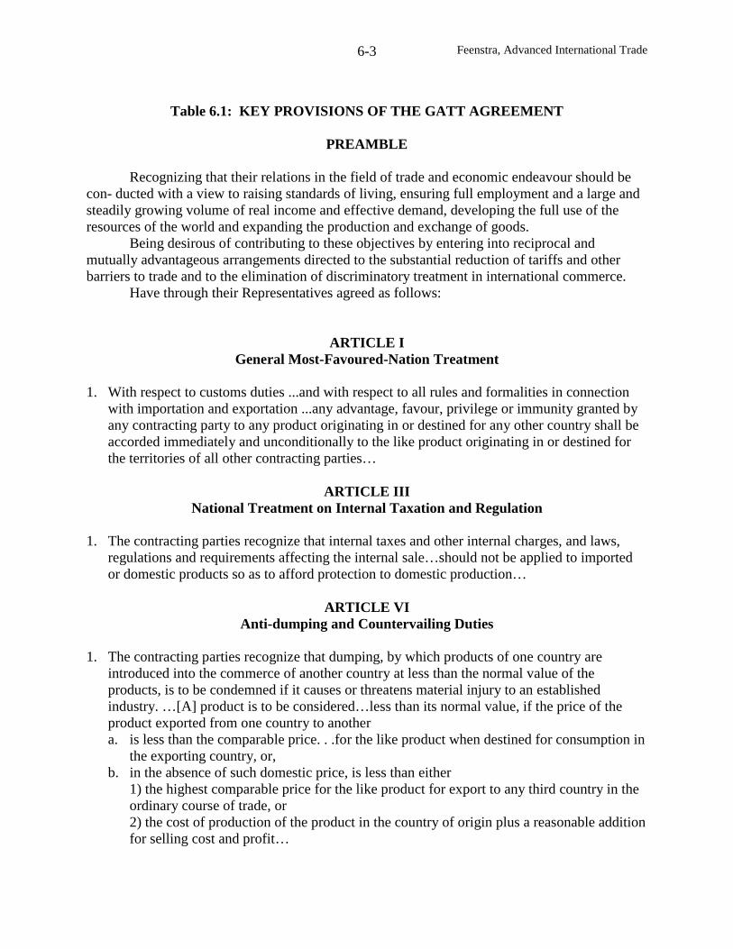
Feenstra, Advanced International Trade6-3
Table 6.1: KEY PROVISIONS OF THE GATT AGREEMENT
PREAMBLE
Recognizing that their relations in the field of trade and economic endeavour should becon- ducted with a view to raising standards of living, ensuring full employment and a large andsteadily growing volume of real income and effective demand, developing the full use of theresources of the world and expanding the production and exchange of goods.
Being desirous of contributing to these objectives by entering into reciprocal andmutually advantageous arrangements directed to the substantial reduction of tariffs and otherbarriers to trade and to the elimination of discriminatory treatment in international commerce.
Have through their Representatives agreed as follows:
ARTICLE IGeneral Most-Favoured-Nation Treatment
1. With respect to customs duties ...and with respect to all rules and formalities in connectionwith importation and exportation ...any advantage, favour, privilege or immunity granted byany contracting party to any product originating in or destined for any other country shall beaccorded immediately and unconditionally to the like product originating in or destined forthe territories of all other contracting parties…
ARTICLE IIINational Treatment on Internal Taxation and Regulation
1. The contracting parties recognize that internal taxes and other internal charges, and laws,regulations and requirements affecting the internal sale…should not be applied to importedor domestic products so as to afford protection to domestic production…
ARTICLE VIAnti-dumping and Countervailing Duties
1. The contracting parties recognize that dumping, by which products of one country areintroduced into the commerce of another country at less than the normal value of theproducts, is to be condemned if it causes or threatens material injury to an establishedindustry. …[A] product is to be considered…less than its normal value, if the price of theproduct exported from one country to anothera. is less than the comparable price. . .for the like product when destined for consumption in
the exporting country, or,b. in the absence of such domestic price, is less than either
1) the highest comparable price for the like product for export to any third country in theordinary course of trade, or2) the cost of production of the product in the country of origin plus a reasonable additionfor selling cost and profit…
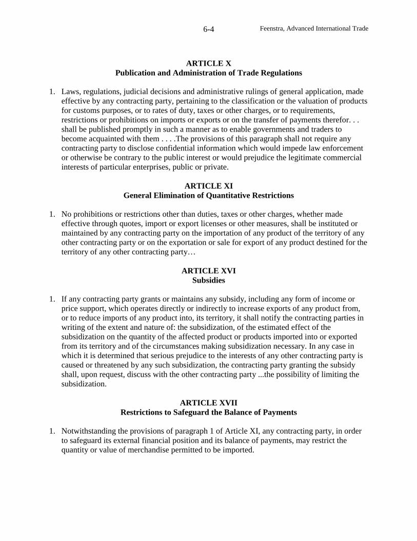
Feenstra, Advanced International Trade6-4
ARTICLE XPublication and Administration of Trade Regulations
1. Laws, regulations, judicial decisions and administrative rulings of general application, madeeffective by any contracting party, pertaining to the classification or the valuation of productsfor customs purposes, or to rates of duty, taxes or other charges, or to requirements,restrictions or prohibitions on imports or exports or on the transfer of payments therefor. . .shall be published promptly in such a manner as to enable governments and traders tobecome acquainted with them . . . .The provisions of this paragraph shall not require anycontracting party to disclose confidential information which would impede law enforcementor otherwise be contrary to the public interest or would prejudice the legitimate commercialinterests of particular enterprises, public or private.
ARTICLE XIGeneral Elimination of Quantitative Restrictions
1. No prohibitions or restrictions other than duties, taxes or other charges, whether madeeffective through quotes, import or export licenses or other measures, shall be instituted ormaintained by any contracting party on the importation of any product of the territory of anyother contracting party or on the exportation or sale for export of any product destined for theterritory of any other contracting party…
ARTICLE XVISubsidies
1. If any contracting party grants or maintains any subsidy, including any form of income orprice support, which operates directly or indirectly to increase exports of any product from,or to reduce imports of any product into, its territory, it shall notify the contracting parties inwriting of the extent and nature of: the subsidization, of the estimated effect of thesubsidization on the quantity of the affected product or products imported into or exportedfrom its territory and of the circumstances making subsidization necessary. In any case inwhich it is determined that serious prejudice to the interests of any other contracting party iscaused or threatened by any such subsidization, the contracting party granting the subsidyshall, upon request, discuss with the other contracting party ...the possibility of limiting thesubsidization.
ARTICLE XVIIRestrictions to Safeguard the Balance of Payments
1. Notwithstanding the provisions of paragraph 1 of Article XI, any contracting party, in orderto safeguard its external financial position and its balance of payments, may restrict thequantity or value of merchandise permitted to be imported.
Feenstra, Advanced International Trade6-5
ARTICLE XIXEmergency Action on Imports of Particular Products
1. (a) If, as a result of unforeseen developments and of the effect of the obligations incurred bya contracting party under this Agreement, including tariff concessions, any product is beingimported into the territory of that contracting party in such increased quantities and undersuch conditions as to cause or threaten serious injury to domestic producers in that territoryof like or directly competitive products, the contracting party shall be free, in respect of suchproduct, and to the extent and for such time as may be necessary to prevent or remedy suchinjury, to suspend the obligation in whole or in part or to withdraw or modify theconcession…
ARTICLE XXIVTerritorial Application-Frontier Traffic-Customs Unions and Free-Trade Areas
4. The contracting parties recognize the desirability of increasing freedom of trade by thedevelopment, through voluntary agreements, of closer integration between the economies ofthe countries party to such agreements. They also recognize that the purpose of a customsunion or of a free-trade area should be to facilitate trade between the constituent territoriesand not to raise barriers to the trade of other contracting parties with such territories.
5. Accordingly, the provisions of this Agreement shall not prevent [the formation of customsunions and free-trade areas, provided that:]a …the duties [with outside parties] shall not on the whole be higher or more restrictive thanthe general incidence of the duties…prior to the formation…
Source: David B. Yoffie and Benjamin Gomes-Casseres, 1994, International Trade andCompetition. New York, McGraw Hill, pp. 420-422.
Feenstra, Advanced International Trade6-6
the world, with zero tariffs internally, this is called a customs union. The European Economic
Community (EEC) is one example of a customs union, and another is MERCOSUR, established
in 1995, which includes Argentina, Brazil, Paraguay and Uruguay. In contrast, if the group of
countries maintains their own tariffs against the rest of the world, with zero tariffs internally,
then this is called a free trade area. Examples of free trade areas are the Canada-U.S. Free Trade
Agreement (CUSFTA) of 1989, which later led to the North American Free Trade Agreement
(NAFTA) of 1994, which consists of Canada, the United States and Mexico. Both customs
unions and free trade areas violate the MFN principle, since the countries within the union or
area are treated differently from those outside. But such agreements are permitted under Article
XXIV of the GATT, provided that “the duties [with outside parties] shall not on the whole be
higher or more restrictive than the general incidence of the duties . . .prior to the formation.”
Because customs unions and free trade areas involve only partial elimination of tariffs,
they can lead to unexpected results: as pointed out by Viner (1950), the countries left out of the
union and even the countries inside the union can become worse off. We discuss this possibility
at the end of the chapter, and identify conditions under which this outcome can be avoided, as in
Kemp and Wan (1976). This also provides us with an important area for empirical research, i.e.
measuring the gains and losses from preferential agreements, of which there have been an
increasing number in recent years. We discuss several empirical studies: Grinols (1984) on
Britain’s membership in the EEC; Clausing (2001) and Romalis (2002) on trade creation and
diversion due to CUSFTA and NAFTA; and Chang and Winters (2002) on the terms of trade
effects of MERCOSUR. We conclude the chapter by extending the results to include imperfect
competition and increasing returns to scale, and also discussing the welfare effects of regional
agreements under these conditions.
Feenstra, Advanced International Trade6-7
Lump Sum Transfers
Our discussion of lump sum transfers follows Dixit and Norman (1980, pp. 76-78). We
want to distinguish the various consumers in the economy, so we index them by h=1,…,H. We
will suppose that individual h has the increasing and quasi-concave utility function )v,c(u hhh ,
where ch
is the N-dimensional vector of consumption, and vh
is the M-dimensional vector of
factor supplies. Under autarky, each consumer maximizes utility subject to the budget
constraint,
haahaa v'wc'p ≤ , (6.1)
where pa
is the autarky vector of commodity prices, and wa
is the autarky vector of factor prices.
The resulting utility for each consumer is )v,c(u hahah .
Summing over all consumption and factor supplies, the total output in the economy is
therefore aH1h
ha yc =∑ = , and the total factor inputs are aH1h
ha vv =∑ = . Of course, the point
)v,y( aa must be feasible for producers, and also optimal at the prices )w,p( aa . We will
assume that the technology for the economy is subject to constant returns to scale. This means
that the payments to factors are exactly equal to the revenue collected, so that profits in the
economy are,
0v'wy'p aaaa =− .
We now consider the free trade equilibrium, which includes a system of lump-sum taxes
or transfers from the government to each individual. We will let Rh
denote the transfer to each
individual h, so that Rh
< 0 is a lump-sum tax. Then the total revenue collected by the
Feenstra, Advanced International Trade6-8
government is hH1h R∑ =− , and we will need to establish that this is non-negative in order for
this system of lump-sum transfers to be feasible.
Denote the equilibrium commodity and factor prices under free trade by (p, w). With
each individual receiving the transfer Rh, the budget constraint is:
hhh Rv'wc'p +≤ . (6.2)
We want to choose a pattern of transfers that allows each individual to be as well off as they
were in autarky. To this end, consider the following system:
haahaah v)'ww(c)'pp(R −−−= . (6.3)
To interpret this, if a price for a commodity rises going from autarky to free trade, the
government will subsidize each individual by the price rise times their autarky consumption.
Conversely, if the earnings of a factor rises going from autarky to free trade, the government will
tax each individual by the wage increase times their autarky factor supply. The goal of this
transfer system is to ensure that all individuals can still afford their autarky choices )v,c( haha .
To see that this is indeed the case, substitute these autarky choices into the budget constraint
(6.2), and make use of (6.3), to obtain:
haahahahaahaahaha v'wc'pv)ww(c)'pp(v'wc'p ≤⇔′−−−+≤ .
Since the second equation above is just the individual’s autarky budget constraint in (6.1), we
know that it is satisfied. This proves that the autarky choices )v,c( haha are feasible for the
budget constraint in (6.2) and transfers in (6.3).
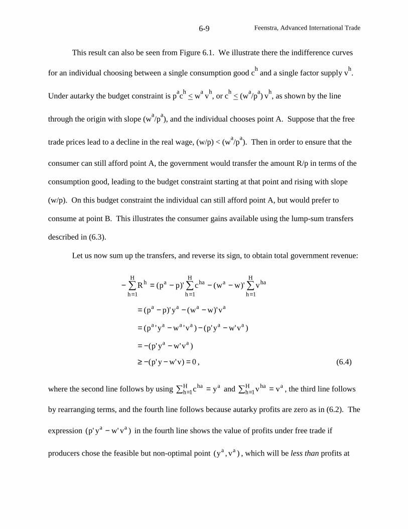
Feenstra, Advanced International Trade6-9
This result can also be seen from Figure 6.1. We illustrate there the indifference curves
for an individual choosing between a single consumption good ch
and a single factor supply vh.
Under autarky the budget constraint is pac
h< w
av
h, or c
h< (w
a/p
a) v
h, as shown by the line
through the origin with slope (wa/p
a), and the individual chooses point A. Suppose that the free
trade prices lead to a decline in the real wage, (w/p) < (wa/p
a). Then in order to ensure that the
consumer can still afford point A, the government would transfer the amount R/p in terms of the
consumption good, leading to the budget constraint starting at that point and rising with slope
(w/p). On this budget constraint the individual can still afford point A, but would prefer to
consume at point B. This illustrates the consumer gains available using the lump-sum transfers
described in (6.3).
Let us now sum up the transfers, and reverse its sign, to obtain total government revenue:
∑∑∑===
−−−=−H
1h
haaH
1h
haaH
1h
h v)'ww(c)'pp(R
aaaa v)'ww(y)'pp( −−−=
)v'wy'p()v'wy'p( aaaaaa −−−=
)v'wy'p( aa −−=
0)v'wy'p( =−−≥ , (6.4)
where the second line follows by using aH1h
ha yc =∑ = and aH1h
ha vv =∑ = , the third line follows
by rearranging terms, and the fourth line follows because autarky profits are zero as in (6.2). The
expression )v'wy'p( aa − in the fourth line shows the value of profits under free trade if
producers chose the feasible but non-optimal point )v,y( aa , which will be less than profits at
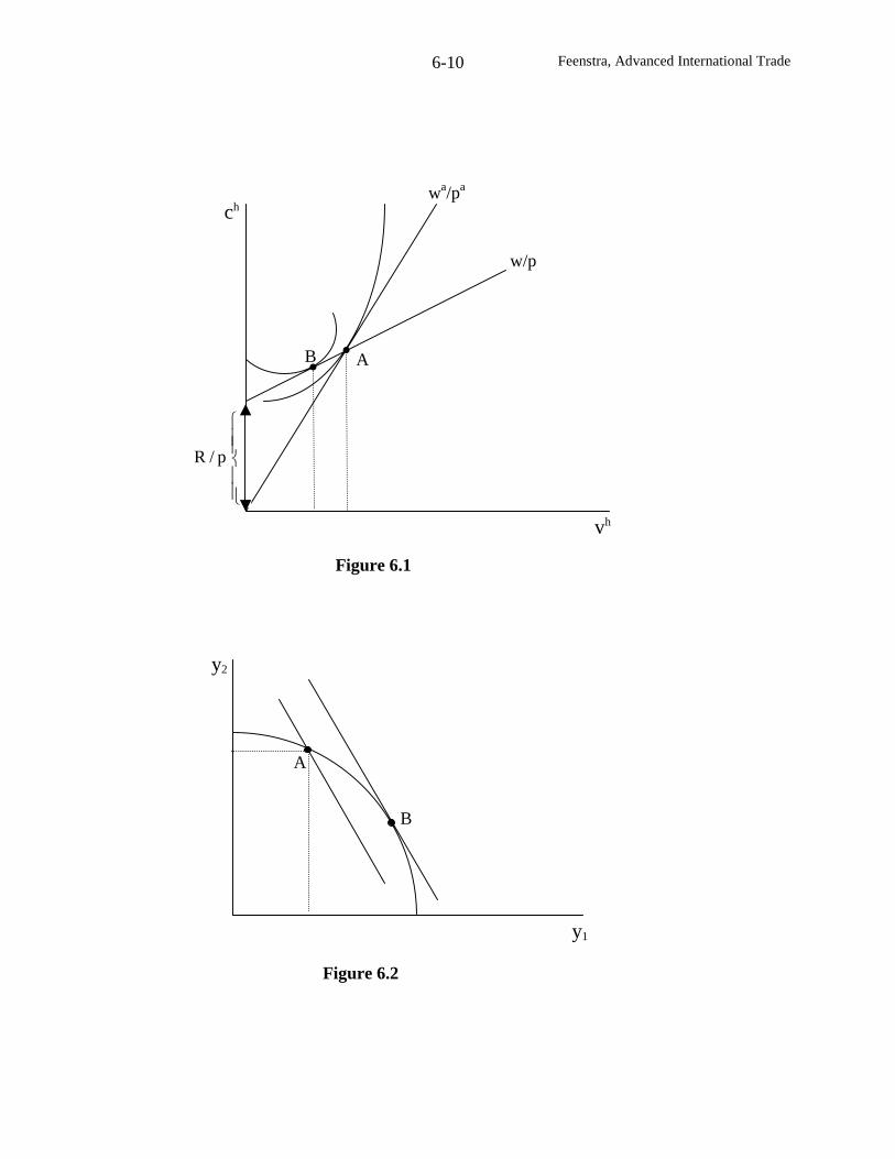
Feenstra, Advanced International Trade6-10
AB
vh
chwa/pa
p/R
Figure 6.1
w/p
A
y2
y1
B
Figure 6.2
Feenstra, Advanced International Trade6-11
the optimal point (y,v), and these profits are zero from constant returns to scale. This establishes
the final line.
Therefore, we see that hH1h R∑ =− > 0, so this system does not cost the government
anything: the lump-sum taxes collected from those gaining from trade are more than enough to
cover the losses to those harmed by trade. No one is harmed by the move to free trade, and
there will generally be gains of two sorts: the consumption gains shown in Figure 6.1 from
consuming at a point different from autarky; and the efficiency gains that arise when the value of
output )v'wy'p( − is strictly greater than )v'wy'p( aa − , so that the inequality on the last line of
(6.4) is strict. To understand this source of gains, consider a special case where the factor
supplies chosen by consumers do not change, so that the total factor inputs v are fixed. Then we
have that y'pv'wv'w a == , so that the revenue collected by the government in (6.4) is:
hH1h R∑ =− = aaa y'py'p)v'wy'p( −=−− . (6.4’)
In Figure 6.2, for example, suppose that the autarky equilibrium is at point A and the free
trade production point at B. Then the revenue collected by the government is exactly the
difference between the value of production at these points (with prices p), or the difference
between the two budget lines that are drawn. With this revenue given back to consumers, they
enjoy gains for that reason in addition to the consumption gains illustrated in Figure 6.1.
As appealing as these results on Pareto gains from trade are, the idea of using lump-sum
transfers is not realistic because this policy requires too much information to implement. This
can be seen from (6.3), where the transfers require knowledge of each individual’s autarky
consumption and factor supplies. Suppose that the government announced a plan to collect this
Feenstra, Advanced International Trade6-12
information using a survey, and then implement the transfers in (6.3). Given knowledge of the
formula used in (6.3), people would then have an incentive to change their consumptions and
factor supplies so as to have more beneficial values of )v,c( haha recorded in the survey, and
therefore get more transfers, thereby leading to a government budget deficit. This is an example
of an incentive compatibility problem: the attempt to implement a policy would lead individuals
to not truthfully report the information needed.
There are two possible solutions to such a problem. The first, which we describe next, is
to use policy instruments that do not require individual information. A second solution is to
build into the policy itself an incentive for people to tell the truth. The transfers in (6.3) certainly
will not do this: everyone would claim that they had consumed more of goods whose prices
increased from autarky to trade, and supplied more of factors whose wages fell. But perhaps
there is some other system of transfers that would lead to truthful reporting of individual
information, and is therefore incentive compatible, while at the same time leading to Pareto
gains. This topic is explored in Feenstra, McMillan and Lewis (1990), Feenstra and Lewis
(1991a) and Facchini and Willmann (1999), but is beyond the scope of the present chapter.
Commodity Taxes and Subsidies
Dixit and Norman (1980, pp. 79-80) and Dixit (1986) have proposed a system of
commodity taxes and subsidies that are designed to achieve Pareto gains from trade, without
requiring individual information (or at least, requiring much less information). Specifically, their
idea is to allow good and factor prices for producers to move to their free trade levels, but hold
good and factor prices for consumers fixed at their autarky levels. Let us denote the autarky
prices by (pa, w
a) and the equilibrium prices with free trade (and the commodity tax/subsidies in
place) by (p, w). We let firms face these free trade prices, and set the vector of consumer taxes
Feenstra, Advanced International Trade6-13
on goods at )pp( a − , and the vector of consumer subsidies on factors at )ww( a − . It follows
that consumers face the price vector )w,p( aa , which is the same as in autarky. Therefore, they
would make exactly the same decisions as in autarky, and achieve their autarky utility
)v,c(u hahah .
Next, we check the government budget. The revenue collected from this system of
commodity taxes and subsidies equals:
∑∑==
−−−H
ih
haaH
ih
haa v)'ww(c)'pp( aaaa v)'ww(y)'pp( −−−= . (6.5)
Notice that this is identical to the expression in (6.4), and is therefore non-negative for exactly
the same reasons. As we discussed in (6.4’) and Figure 6.2, this expression is strictly positive
whenever there are efficiency gains from having producers face free trade rather than autarky
prices. If this is the case, then the government redistributes this revenue back to consumers as a
“poll subsidy” (i.e. an equal amount to each person). In that way, all consumers receive more
than their autarky utility level, and Pareto gains from trade are achieved!
This system of commodity taxes and subsidies just requires information on the goods and
factor prices (pa, w
a) and (p, w), which is obviously much less than required to compute the
lump-sum transfers in (6.3). On the other hand, it should not be thought that the factor price
information is always available. If we can think of the quantity of a factor supplied as measuring
effort rather than just hours worked, then the factor prices need to be measured per unit of effort.
If effort is not observed, then neither are the true prices or factor supplies. To state this problem
differently, a worker who was guaranteed his autarky wage even when trade is opened would no
longer have an incentive to work hard. Thus, there is again an incentive compatibility problem
Feenstra, Advanced International Trade6-14
related to the collection of factor prices whenever individual’s effort cannot be observed. A
similar problem occurs for workers paid annual salaries rather than wages, so that we observe
their income wvh
rather than wages w. In this case, we would have to infer their factor supply
(or effort level) vh
before knowing their wage w.1
A second potential difficulty with this system of commodity taxes and subsidies occurs
when individuals have moving costs. To model this, suppose that the vector of factor supplies vh
appearing in the utility function is indexed by the location where the individual works. That is, if
the economy has M primary factors and L locations, the vector vh
is of dimension LM rather than
M. An individual who is indifferent between working in one location versus the other would
have indifference curves that are linear between these two factor supplies: when offered a wage
slightly higher in one location, the individual would shift entirely there. But if instead the utility
function uh(c
h, v
h) is strictly quasi-concave, then this individual would not be willing to shift
between locations when wages are unchanged. This formulation is a simple way to capture the
idea that individuals have preferences over where to work and psychic costs to relocating.
Notice that it is still consistent with the Arrow-Debreu general equilibrium model, which allows
goods or factor to be indexed by location.
What are the implications of this for the system of commodity tax and subsidies proposed
by Dixit and Norman (1980)? Suppose that we use the factor subsidies to bring all individuals
1 This difficulty occurs especially for specific factors in an industry, where at most we would observe their totalincome but not their wage. This is an important example because of our earlier assumption that the technology ofthe economy has constant returns to scale. Suppose instead that the technology had decreasing returns, in which casethe revenue earned exceeds the sum of factor payments, so (6.2) does not hold. Then define the difference betweenrevenue earned and factor payments as the income of a hypothetical fixed factor of production, so that includingpayments to this fixed factor, we have constant returns and (6.2) holds again. Then we would only observe incomeof this fixed factors, and not the separate wage and factor supply.
Feenstra, Advanced International Trade6-15
back to their autarky factor prices. Since vh
is indexed by location, and uh(c
h, v
h) is strictly
quasi-concave, this means that individuals have a unique choice of where to work, and are
unwilling to shift between locations at the autarky wages. Assume that the various goods in the
economy are produced at different locations. Then opening the economy up to trade, but holding
wages fixed at wa, means that it is impossible for the economy to shift from a point like A to
point B in Figure 6.2: if workers are unwilling to move between industry/locations at constant
wages, the economy will be stuck at point A despite the change in producer prices. It is
appropriate to think of the preferences over locations, combined with wages fixed at their
autarky level, as introducing a “kink” into the production possibility frontier at point A, as
illustrated by the dashed lines in Figure 6.2. Because production no longer changes in response
to the free trade prices, there are no efficiency gains and government revenue in (6.5) is zero. In
this case, the scheme of commodity tax/subsidies proposed by Dixit and Norman fail to achieve
any gains.
Feenstra and Lewis (1994) have investigated this case, and argue that moving subsidies
can restore Pareto gains through subsidizing workers to move between industry/locations. An
example of such subsidies in the United States is Trade Adjustment Assistance (TAA). As
described in Richardson (1982), this program was established in the United States under the
Trade Act of 1974 to compensate workers in industries that experienced unemployment due to
import competition. It was used heavily by auto workers during the U.S. recession of the early
1980s, for example. However, it has often been the case that workers using this program have
not shifted into new jobs, but instead used TAA as an income supplement during their period of
unemployment (see the evidence in Aho and Bayard, 1984). This was especially true for the
automobile workers laid off in Detroit in 1979 and 1980: many of them simply collected the
Feenstra, Advanced International Trade6-16
TAA benefits and when the automobile industry recovered, they returned to their former jobs.
Findings such as this eventually led the U.S. Congress to realize that the program was not
encouraging relocation of workers, and its funding was cut drastically. A much smaller TAA
program was later implemented along with NAFTA in 1994, and this program requires job re-
training (see Irwin, 2002, pp. 106-110).
There is some theoretical validity to the idea that a TAA program is worthwhile only if it
leads to the relocation of workers between industries. In terms of Figure 6.2, the economy
achieves production gains of going from point A to point B only if workers are willing to move
between industry/locations: simply giving income supplements to workers but having
production remain at point A cannot be a self-financing policy. Furthermore, it is essential that
workers move in the “right” direction, i.e. towards those industries whose international prices
have increased, or from point A to point B in Figure 6.2. Feenstra and Lewis (1994) show how
a program of moving subsidies can be designed to achieve this goal, so that in conjunction with
the commodity taxes proposed by Dixit and Norman, the program achieves Pareto gains and is
self-financing.2
As a final example of how the commodity tax/subsidies proposed by Dixit and Norman
relate to actual policies, consider the case of the unification of East and West Germany. As
described by Akerlof, et al (1991, p. 1): “At midnight on June 30, 1990, German economic,
monetary, and social union occurred: the mark of the German Democratic Republic [East
Germany] was replaced by the deutsche mark; trade barriers were lifted; legal, tax, and social
2 A richer comparison of trade adjustment assistance with wage and employment subsidies is provided byDavidson and Matusz (2002), in a model where workers search for new jobs and therefore have temporary spells ofunemployment. They argue that temporary wage subsidies (in industries when workers should be moving) andtemporary employment subsidies (in industries that workers have difficulty leaving) are preferable to adjustmentassistance and can be used to achieve Pareto gains.
Feenstra, Advanced International Trade6-17
insurance system were harmonized; and all existing barriers to capital and labor movement were
removed.” The replacement of the mark with the deutsche mark at par, and the pressure from
labor unions to achieve wage parity between the East and West, meant that companies in former
East Germany were faced with wages that were far above their market levels. Indeed, Akerlof,
et al (1991) estimate that only 8% of former East German conglomerates would have been
profitable at those high wages. In the absence of government intervention, it could be expected
that wages in the industries located in Eastern Germany would have fallen dramatically, and in
the absence of this, severe bankruptcy and unemployment would result.
The government supported the increase of wages in the East to the level of those in the
West in order to avoid migration out of the East. Thus, not only did government policies
explicitly allow workers in former Eastern Germany to maintain their standard of living from
unification, these policies encouraged an increase in living standards (to the level of Western
wages) in order to avoid migration. At the same time, it was expected that workers in former
West Germany should not be harmed by unification. This historical episode is therefore a
perfect example of an attempt to achieve Pareto gains from trade in practice.
How could such gains be achieved in the face of non-market clearing wages in East
Germany, combined with unemployment? The answer proposed by Akerlof, et al (1991, p. 4) is
that “flexible employment bonuses” or wage subsidies should be used in the East:
So far…the package of policies that has been enacted fails to deal realistically with the
questions of how to preserve existing jobs, how to speed new job creation, and how to
make existing companies viable enough to be privatized. The major problem is that
wages in the East are too high for most former state-owned enterprises to cover their
costs. High wage also deter new investment. This creates an obvious need for
governmental measures to close the gap between the high private cost of labor, caused by
Feenstra, Advanced International Trade6-18
high Eastern wages, and the low marginal product of labor, caused by outmoded capital
and technology. We propose a program of self-eliminating flexible employment
bonuses… to eliminate this gap. Our analysis shows that such a program would give
many workers a chance to keep their jobs and would also raise the level of new job
creation through faster private investment. According to our estimates, even deep wage
subsidies (for example, an employment bonus equal to 75 percent of current wages)
would have very low budgetary costs. They might even reduce the budget deficits –
largely for the same reason that infrastructure investment is not costly: the government is
already committed to a high level of income support even if workers are unemployed.
Thus, by subsidizing workers in East Germany the government could save enough income from
unemployment benefits that the policy could be self-financing. This is very similar to the
commodity tax/subsidies proposed by Dixit and Norman (1980), and shows how wage subsidies
have an potentially important role to play in an actual attempt to achieve Pareto gains from
trade.3
Partial Reform of Tariffs
We now consider a country that undertakes a partial reform of its tariff structure, moving
from one situation of restricted trade (possible autarky) to another. This is a very realistic
example, since countries undertake partial reform of their tariff frequently (though it is often
done in conjunction with tariff reforms abroad). The question is: are individuals better off in
this country or not? To answer this, we make use of the lump-sum transfers as a means to
compensate individuals for this move, so we will need to check whether the government budget
constraint allows this compensation or not. While the use of lump-sum transfers is not realistic,
3 Unfortunately, the wage subsidy proposal of Akerlof, et al (1991) was not followed in Germany, and migrationfrom east to west continues to be a policy issue. Interestingly, Phelps (1997) also proposes a system of wagesubsidies to offset the fall in wages for unskilled workers in the United States, whose wages have fallen during the1980s and 1990s, as discussed in chapter 4.
Feenstra, Advanced International Trade6-19
the reader should think of this as simply a method to evaluate the desirability of the tariff reform,
i.e., if the tariff reform combined with lump-sum transfers could make everyone better off, then
we accept the tariff reform itself as a worthwhile policy, even when the transfers are not made.
This criterion for evaluating a reform is called the “compensation principle” (see Chipman,
1987). Our analysis will follow that in Grinols and Wong (1991), and also Ju and Krishna
(2000a), though the latter authors also show how the results can be extended to non-lump-sum
transfers, using commodity tax and subsidies as in Dixit and Norman (1980) and Dixit (1986).4
To set up our notation, let the domestic price vector for consumers and producers be
denoted by p = p* + t, where p* is the vector of world prices, and t is the vector of trade taxes
and subsidies. Notice that ti > 0 for an imported good indicates a tariff (raising the domestic
price above the world price), whereas ti < 0 for an imported good indicates a subsidy.
Conversely, ti > 0 for an exported good indicates a subsidy (since firms receive pi* + ti from
exporting, the domestic price would also have to rise by the same amount), while ti < 0 for an
exported good indicates a tax. It follows that the total revenue collected by the government from
the trade tax/subsidies is )yc('t − , where ∑ == H1h
hcc is total consumption and y is the output of
the economy at the prices p. For convenience, let us denote the import vector as m = c – y, so
that revenue collected is simply m't .
We compare two different trade tax/subsidies t0
and t1, with the equilibrium domestic
price vectors p0
= p*0
+ t0
and p1
= p*1
+ t1. We stress that the world price p* changes in these
two situations, and in general, these are endogenously determined by the tariffs chosen at home.
4 An alternative approach to the piecemeal reform of tariffs, relying on small reforms and using calculus, isprovided in Diewert et al (1989), Ju and Krishna (2000b) and Turunen-Red and Woodland (1991, 2000).
Feenstra, Advanced International Trade6-20
More generally, our setup allows for a change in tariffs abroad simultaneously with those at
home, as part of a bilateral or multilateral tariff reform.
Our argument will follow the earlier discussion of lump-sum compensation quite closely.
In the initial situation, we suppose that consumers maximize utility subject to their budget
constraints,
H/)m't(v'wc'p 000h00h0 +≤ , (6.6)
where p0
is the autarky vector of commodity prices, w0
is the autarky vector of factor prices, and
we include the redistributed tariff revenue H/m't 00 , where H is the number of consumers. The
resulting utility for each consumer is )v,c(u 0h0hh .
Summing over all consumption and factor supplies, the total consumption in the economy
is therefore 0H1h
0h cc =∑ = , and the total factor inputs are 0H1h
0h vv =∑ = . Firms will be
maximizing profits at the equilibrium prices )w,p( 00 , resulting in the outputs y0
and factor
demands v0. Again, we assume constant returns to scale so that the resulting profits are zero,
0v'wy'p 0000 =− . Imports in this equilibrium are m0
= c0
– y0, so the revenue collected is
00 m't , which has been transferred back to consumers in (6.6).
After the tariff reform, domestic prices change to p1
= p*1
+ t1, and the revenue collected
from the trade tax/subsidies becomes 11 m't . We denote the transfer to consumers by Rh, which
may differ from just the revenue 11 m't . The budget constraint for consumers is,
hh1h1 Rv'wc'p +≤ . (6.7)

Feenstra, Advanced International Trade6-21
Our goal is to identify conditions under which the government can compensate individuals for
the change in prices, and at the same time, balance the government budget. Using a similar
system of lump-sum transfers that we considered earlier, this can be achieved by:
Theorem (Grinols and Wong, 1991; Ju and Krishna, 2000a)
When the prices change from p0
= p*0
+ t0
to p1
= p*1
+ t1, suppose that the government
transfers the following amount to each individual:
H/)m't(v)'ww(c)'pp(R 000h010h01h +−−−= . (6.8)
Provided that 0)mm('tm)'*p*p( 011010 ≥−+− , then no individual is worse off and the
government budget is balanced.
Proof:
Substituting the transfers in (6.8) into individual’s budget constraint (6.7), we can confirm that
the initial choices )v,c( 0h0h are still feasible:
.H/)m't(v'wcp
H/)m't(v)'ww(c)'pp(v'wc'p
000h00h0
000h010h010h10h1
+≤⇔
+−−−+≤(6.9)
Since the second equation shown is just the initial budget constraint in (6.6), the initial choices
)v,c( 0h0h are feasible and utility is at least )v,c(u 0h0hh .
To check the government budget, we subtract the transfers from the tariff revenue,
obtaining,
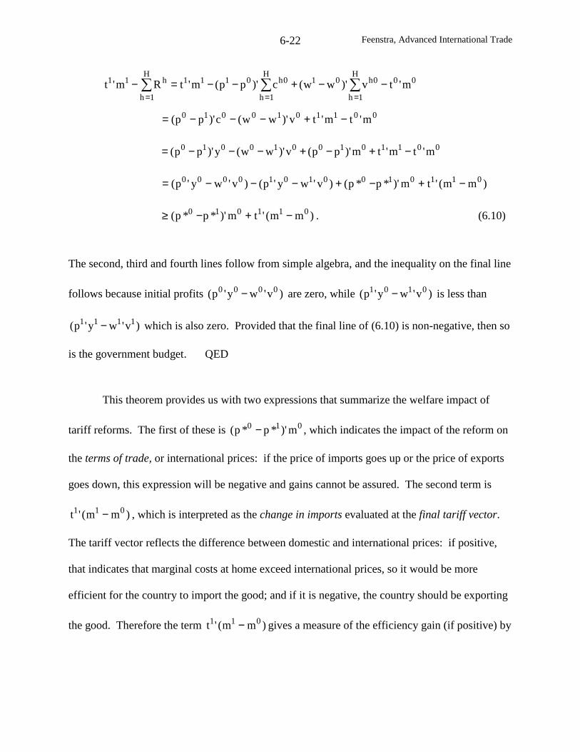
Feenstra, Advanced International Trade6-22
00H
1h
0h01H
1h
0h0111H
1h
h11 m'tv)'ww(c)'pp(m'tRm't −−+−−=− ∑∑∑===
0011010010 m'tm'tv)'ww(c)'pp( −+−−−=
0011010010010 m'tm'tm)'pp(v)'ww(y)'pp( −+−+−−−=
)mm('tm)'*p*p()v'wy'p()v'wy'p( 01101001010000 −+−+−−−=
)mm('tm)'*p*p( 011010 −+−≥ . (6.10)
The second, third and fourth lines follow from simple algebra, and the inequality on the final line
follows because initial profits )v'wy'p( 0000 − are zero, while )v'wy'p( 0101 − is less than
)v'wy'p( 1111 − which is also zero. Provided that the final line of (6.10) is non-negative, then so
is the government budget. QED
This theorem provides us with two expressions that summarize the welfare impact of
tariff reforms. The first of these is 010 m)'*p*p( − , which indicates the impact of the reform on
the terms of trade, or international prices: if the price of imports goes up or the price of exports
goes down, this expression will be negative and gains cannot be assured. The second term is
)mm('t 011 − , which is interpreted as the change in imports evaluated at the final tariff vector.
The tariff vector reflects the difference between domestic and international prices: if positive,
that indicates that marginal costs at home exceed international prices, so it would be more
efficient for the country to import the good; and if it is negative, the country should be exporting
the good. Therefore the term )mm('t 011 − gives a measure of the efficiency gain (if positive) by
Feenstra, Advanced International Trade6-23
attracting imports towards the highest-tariff sectors, or loss (if negative). Thus, policies to raise
welfare must avoid adverse terms of trade or efficiency effects to ensure Pareto gains.
Notice that the term )mm('t 011 − can also be interpreted as the change in tariff revenue
evaluating at the final tariff vector. In some cases, this will equal the overall change in tariff
revenue. For example, suppose that a small country starts with prohibitive tariffs on some goods,
and then moves to free trade in those goods. Since they have zero tariff revenue before and after
the change, the term )mm('t 011 − shows what happens to revenue collected on the other goods,
whose tariffs are unchanged. If tariff revenue falls, then we cannot be sure that the country
gained from the partial movement towards free trade. Working with a one-consumer small
economy, Ohyama (1972) was the first to identify the sufficient condition that tariff revenue
(evaluated at the final tariff vector) must rise to ensure gains.
Two special cases of the above theorem can be noted:
Corollary
Applying the transfers to individuals as in (6.8):
(a) Starting in autarky and moving to trade with tariffs and subsidies makes no one worse off
provided that 0m't 11 ≥ ;
(b) For small country with constant world prices, p*0
= p*1, a change in tariffs and subsidies
makes no one worse off provided that )mm('t 011 − > 0.
In the first case, we set m0
= 0 in the above theorem, and see that the criterion to achieve
Pareto gains is just 0m't 11 ≥ , i.e. the tariffs and subsidies must raise non-negative revenue.
Ohyama (1972) described this condition as “self-financing” tariffs. The result in Corollary (a) is
Feenstra, Advanced International Trade6-24
interpreted as saying that “some trade is better than no trade.” If we suppose that the second
situation has free trade, t1=0, then the condition in Corollary (a) is clearly satisfied and this result
is interpreted as “free trade is better than autarky” (Samuelson, 1962; Kemp, 1962). Corollary
(b) considers a “small country,” facing fixed world prices, and shows that a tariff reform will
raise welfare provided that the efficiency effects are non-negative. Again, if we suppose that the
second situation has free trade, t1=0, then the condition in Corollary (b) is clearly satisfied and
this result can be interpreted as “free trade is better than restricted trade for a small country.” We
will provide another demonstration of this result in the next chapter.
Regional Trade Agreements
We now extend our results to the case where a group of countries decides to pursue free
trade internally, while maintaining tariffs against the rest of the world. Under a customs union,
the countries involved choose a common external tariff with the rest of the world, whereas under
a free trade area the countries maintain different tariffs on imports from the rest of the world.
Let us consider the customs union case first, since it is easier.
The analysis of customs unions dates back to Viner (1950), who introduced the terms
“trade creation” versus “trade diversion.” Trade creation refers to a situation where two
countries within the customs union begin to trade with each other, whereas formerly they
produced the good in question for themselves. In terms of Corollary (a) above, the countries go
from autarky (in this good) to trading with zero tariffs, and they both gain. Trade diversion, on
the other hand, occurs when two countries begin to trade within the union, but one of these
countries had formerly imported the good from outside the union. We may presume that the
importing country formerly had the same tariffs on all countries, but purchased from outside the
Feenstra, Advanced International Trade6-25
union because that price was lowest. After the union, the country switches its purchases from the
lowest-price to a higher-price country, so in terms of Corollary (b) there is a negative efficiency
effect, and the country could lose from joining the union.
To verify these results more formally, we need to expand our notation to incorporate the
customs union. In our analysis above we had implicitly assumed that each country i had a single
tariff vector tiapplied against all other countries. This is no longer the case: countries in the
union will face zero tariffs among themselves, and still maintain the same external tariff with
respect to outside countries. An easy way to capture this is to index goods by their region of
origin and their region of destination. That is, let the first N goods denote those produced in the
union and sent to the union; the next N goods are produced outside the union and sent outside the
union; the next N are produced in the union and sent outside the union; and the last N are
produced outside the union and sent into the union. In total we therefore have 4N goods, but
only the last 2N of these involve trade between the union and outside countries. This treatment of
goods still is consistent with the Arrow-Debreu model, where goods can be indexed by location.5
With this notation, the above Theorem and Corollary continue to hold. For a union
country i, the first N tariffs are zero, the second N tariffs are irrelevant (since these goods are
traded between nonunion countries), and the last 2N tariffs are equalized for all countries of the
union. We will denote this post-union tariff vector by t1. Notice that with zero tariffs on
countries within the union, the term )mm('t 0i1i1 − measures the change in tariff revenue for
country i’s imports from outside the union. Trade diversion means that country i switches from
the lowest-price supplier from outside the union (where tariff revenue is collected) to another
5 Note that if consumers are indifferent between a good coming from two locations, then the indifference curvesbetween these locations are linear.
Feenstra, Advanced International Trade6-26
supplier within the union (with no tariff revenue), so that 0)mm('t 0i1i1 <− and tariff revenue
has fallen. Therefore, country i can be worse off. This result illustrates what is called a “second
best” problem: by eliminating its tariffs with all other countries, a small country would
necessary be better off, but by only going partway towards this goal (eliminating tariffs with the
union countries only), there is no guarantee of gains.
This outcome made it seem like no general result on the desirability of customs unions
was possible. Remarkably, Kemp and Wan (1976) were still able to obtain such a result. Their
goal was to ensure that the customs union benefits its members, and also does not harm the rest
of the world. To achieve this, Kemp and Wan used the following rule: the customs union
should keep the world price p* fixed, or equivalently, keep the purchases from the rest of the
world x* fixed. This rule can be contrasted with the criterion used in the WTO on customs
unions. From Article XXIV in Table 6.1, we see that customs unions are “not prevented”
provided that “the duties [with outside parties] shall not on the whole be higher or more
restrictive than the general incidence of the duties. . .prior to the formation.” Thus, the criterion
used in WTO is that the tariffs with respect to countries outside the union should not be higher
than before, whereas the rule used by Kemp and Wan is that the trade with respect to outside
countries is not affected by the formation of the customs union. The Kemp-Wan rule is the
correct one to avoid losses, not the existing WTO criterion.
To develop the result of Kemp and Wan, let us denote the countries in the customs union
by i=1,…,C. Prior to the union they have tariffs 0it . We let p*0
denote the world prices in this
equilibrium, and 0im denote the import vector of country i. Let the net export vector of the rest
of the world be denoted by x*( p*0). Notice that this vector is zero for the first 2N goods (which
Feenstra, Advanced International Trade6-27
refer to trade strictly inside or outside the union), and potentially non-zero otherwise. Summing
imports over all countries in the union, the equilibrium condition is:
∑=
=C
1i
00i )*p(*xm . (6.11)
After the customs union the countries involved have a unified tariff t1, the elements of
which are zero for purchases from within-union countries. Let 1im denote the vector of imports
of country i in this situation. Kemp and Wan (1976) prove that there exists a unified tariff
t1which ensures that,
∑=
=C
1i
01i )*p(*xm . (6.12)
The fact that the prices p*0
and exports from the rest of the world x*( p*0
) are unchanged due to
the customs union guarantees that the rest of the world is not affected by it. The question now is
whether the members of the customs union also gain, and whether this requires some transfers
between the countries or not. This is answered by:
Theorem (Kemp and Wan, 1976; Grinols, 1981)
Let the countries i=1,…,C form a customs union, with the common external tariff such that
prices and purchases from the rest of the world are unchanged. Suppose that each country within
the customs union receives the transfers )mm('t 0i1i1 −− from the rest of the union. Then there
is a pattern of lump-sum transfers within each country such that no individual is worse off, and
the government budget in each country is non-negative.
Proof:
Feenstra, Advanced International Trade6-28
Consider the transfers described in (6.8), but applied within each country. It follows that each
consumer in every country of the union can still afford their previous consumption bundles.
Furthermore, noting that prices p* from the rest of the world are fixed, then from (6.10) the
government budget in each country is no less than )mm('t 0i1i1 − . Therefore, each country can
afford to give up this amount (or receive it if negative), and have a non-negative budget. It
remains to be shown that these transfers within the union are self-financing, that is,
.0)mm('tC1i
0i1i1 =−∑ = But this follows immediately from the fact that total union imports are
equal in (6.11) and (6.12), ∑∑ == = C1i
0iC1i
1i .mm QED
It is apparent that the way losses are avoided for the union is by keeping total imports
fixed: in that way, the total tariff revenue (evaluated at post-union external tariffs) is also fixed.
But keeping total imports fixed also means that world prices are fixed, which eliminates any
terms of trade impacts for the union and the rest of the world. Thus, keeping total union imports
fixed immediately satisfies the criterion identified in the earlier theorem: when summed over the
countries of the union, the term )mm('tm)'*p*p( 0i1i10i10 −+− is zero, so the union as a
whole is no worse off. An individual country may experience a loss in their own tariff revenue
of )mm('t 0i1i1 − , but this could be compensated by transfers from other countries within the
union.
It has been more than 25 years since Kemp and Wan demonstrated this result, and in the
meantime, there has been a proliferation of regional agreements under GATT Article XXIV.
Many of these have not been customs unions, but instead, are free trade areas (FTA’s). Is it
possible to extend the Kemp-Wan theorem to cover these? As explained above, FTA’s differ
Feenstra, Advanced International Trade6-29
from customs unions in that the countries involved have their own tariff vector with respect to
the rest of the world. At the same time, tariffs are zero within the union, so goods can be sent
between these countries freely. This means that producer prices must be equalized within the
union, but by virtue of their differing tariffs on outside countries, consumer prices can differ
within the union. It follows that the method of proof used by Kemp and Wan (1976) cannot be
used for free trade areas. Recently, however, Krishna and Panagariya (2002) have developed a
new proof, which shows that Kemp-Wan theorem can indeed be extended to cover FTA’s. Their
approach can be described quite easily using our notation above.
Let x*( p*0) denote the initial net exports from the rest of the world to the countries
planning to form a FTA. Recall that this vector is zero for the first 2N goods (which refer to
trade strictly inside or outside the union), and potentially non-zero otherwise. The approach of
Krishna and Panagariya is to ensure that every country in the FTA has exactly the same trade
with the rest of the world as they did initially. Letting 0im and 1im denote the imports of
country i=1,…,C, which is a member of the FTA, we require that:
0ijm = 1i
jm , for goods j = 2N+1,…,4N. (6.13)
Thus, we require every FTA member import and export the same quantity with the rest of world
as they did before the free trade area. While Krishna and Panagariya do not provide a general
existence result, we can certainly construct examples where there are country-specific tariffs
ensuring that (6.13) holds, and denote these by ti1
, i=1,…,C. Notice that (6.13) implies that
(6.12) still holds, i.e. total net exports from the FTA to the rest of the world equals x*( p*0), its
value initially. So we conclude that the equilibrium world prices are still given by p*0.
Feenstra, Advanced International Trade6-30
Since trade with the outside world is not affected by the FTA, and neither are prices, we
have obtained the result:
Theorem (Krishna and Panagariya, 2002)
Let the countries i=1,…,C form a free trade area, with external tariffs ti1
for each country such
that prices and purchases from the rest of the world are unchanged. Then there is a pattern of
lump-sum transfers within each country such that no individual is worse off, and the government
budget in each country is non-negative.
Proof:
Again we use the transfers described in (6.8) applied within each country. It follows that each
consumer in every country of the FTA can still afford their previous consumption bundle, and
from (6.11), the government budget in each country is no less than )mm('t 0i1i1i − . The first N
elements of ti1
are zero due to free trade within the FTA, and the next N elements of mi0
and mi1
are zero because those goods are produced and delivered outside the FTA. Then (6.13) ensures
that )mm('t 0i1i1i − = 0, so the budget is non-negative in every country i=1,…,C. QED
One feature of FTA’s and the above theorem should be emphasized. Because tariffs with
respect to the rest of world differ between the member countries, outside countries would have
an incentive to export their goods into the lowest-tariff country of the FTA, and then transship it
to other member countries. This type of activity needs to be ruled out to obtain the above
theorem. That is, transshipment through the lowest-tariff country would violate condition (6.13),
which specifies that each country must import the same quantity from outside countries as before
the FTA. More generally, transshipment through the lowest-tariff country would lead to a drop
Feenstra, Advanced International Trade6-31
in tariff revenue for other countries of the FTA, violating the condition to obtain Pareto gains.
To ensure welfare gains, therefore, we need to rule out transshipment of goods not produced in
the FTA.
In practice, restrictions on such transshipment within FTA’s are known as “rules of
origin” (ROO). Within NAFTA, for example, each and every good must be certified as “North
American made” before it can be shipped freely between Mexico, the U.S., and Canada. This
certification is typically made based on the percentage of value added coming from North
American production, or the use of some key input produced in North America. This prevents a
foreign country from exporting into Canada, for example, and then sending the good to the U.S.
or Mexico, unless it had enough further processing to certify it as “North American made.”
Such rules are enormously complex, since they require a specification of the production process
for each and every good. Because the ROO are an artificial restriction on the movement of
goods they are often criticized (see for example, Krishna and Krueger, 1995). But the theorem
of Krishna and Panagariya sheds new light on these practices, since the welfare-improving FTA
depends on their use.6
Evidence on Regional Agreements
The above theorems allow us to conclude that welfare-improving customs unions and
FTA’s exist, but from this we should not infer that regional trade agreements in practice are
necessarily a good thing. The possibility of trade diversion identified by Viner (1950), and any
6 Let us be more careful in this statement. Starting at any FTA, the theorem of Kemp and Wan ensures that there isa customs union that is Pareto superior. But that customs union is not achieved by simply dropping the ROO fromthe FTA; rather, it would require dropping the ROO, changing the external tariffs for all countries to a common levelthat ensures the same total imports from the rest of the world, and also implementing income transfers acrosscountries within the union. If these actions are politically infeasible, then the ROO are needed in order for the FTAto ensure Pareto gains, as in the theorem of Krishna and Panagariya.
Feenstra, Advanced International Trade6-32
changes in the terms of trade, need to be evaluated empirically before judging actual agreements.
More generally, we should be concerned with whether regional trade agreements help or hinder
the movement towards global free trade through multilateral negotiations under the WTO. This
political economy issue will be discussed in chapter 9.
Grinols (1984) was among the first to measure the gains or losses from membership in a
customs union. He examined Britain joining the European Economic Community in 1973. This
meant that Britain had to adopt the common external tariff of the EEC. Not only would this
affect domestic price piin Britain, it could also be expected to have an impact on the foreign
prices p*ifacing Britain, i.e. on its terms of trade. We are recognizing here that the prices
charged by foreign exporting firms are often responsive to a change in tariffs by just one
importing country. This occurs when foreign firms segment their export markets, charging
different prices in each. This behavior is related to imperfect competition, as will be discussed in
the next chapter.
Grinols measured the prices for British exports and imports during the years after its
membership in the EEC. Multiplying these prices by initial quantities gives 0i1i0i m)'*p*p( − ,
or the value of changes in the terms of trade. In every year from 1973-1980, it turned out that the
British terms of trade had fallen from 1972, and the amount of this decline averaged about 2.3%
of British GDP. (This amount include the lost tariff revenue on imports, which automatically
become property of the customs union, and the average drop in the terms of trade without
including tariff revenue was still 1.7% of GDP.)
In order to compensate for this loss, Britain would have needed to obtain some transfer
from the EEC, i.e. the amount )mm('t 0i1i1 − in our discussion above. There was a wide range

Feenstra, Advanced International Trade6-33
of transfers between countries as part of EEC membership, including the Regional Development
Funds (allocated to projects in lower-income regions), special funds in agriculture, coal and steel,
value-added taxes, etc. The net transfers were slightly in Britain’s favor, but not enough to offset
the terms of trade loss, so that summing 0i1i0i m)'*p*p( − + )mm('t 0i1i1 − still gives an average
loss for Britain of 2.26% of GDP annually.
We conclude that the sufficient condition to ensure Britain’s gain from joining the EEC,
i.e. 0i1i0i m)'*p*p( − + )mm('t 0i1i1 − > 0, did not hold. This does not necessarily imply that
Britain was worse off, however, since it still enjoys free trade within the EEC, and so had
efficiency gains on both the consumption and production side for that reason. In Figure 6.1, for
example, these gains are illustrated by the movement from point A to point B. Grinols attempts
to evaluate these gains for Britain and finds that they are quite small. The conclusion is that its
membership in the EEC in 1973 led to a welfare loss that averaged about 2% of GDP annually
through 1980.
One criticism that can be made of Grinols’ methodology is that he simply accepts the
trade prices as data, and presumes that any change from 1972 represents the effect of Britain’s
membership in the EEC. Thus, the terms of trade decline is attributed to Britain’s changing its
external tariff to the common EEC level. This does not allow for any exogenous changes in the
terms of trade due to factors affecting supply and demand on world markets. To control for such
factors, we need to specify prices as functions of the tariffs, as well as other relevant factors.
Using a log-linear regression to estimate prices as a function of tariffs and other factors allows us
to infer the specific impact of the tariff change. This is the approach taken by Chang and
Winters (2002) for MERCOSUR.
Feenstra, Advanced International Trade6-34
Specifically, Chang and Winters (2002) consider prices from various countries (U.S.,
Japan, German, etc.) to Brazil, which is the largest market in MERCOSUR. This customs union
had the effect of eliminating tariffs between Brazil and Argentina, Paraguay and Uruguay, as
well as equalizing their external tariffs. Of interest, then, is the direct effect of the change in the
external tariff of Brazil on the prices charged by foreign firms; as well as the indirect effect of
the elimination of the tariffs between Brazil and Argentina on the prices charged by foreign firms
to Brazil. Both this direct and indirect effect will lead to a terms of trade change for Brazil, as
well as to the countries selling in that market. The regression framework used to measure these
effects draws on Feenstra (1989), as discussed in detail in the next chapter, and specifies prices
as a log-linear function of tariffs and other factors. By pooling data across disaggregate products
and years, Chang and Winters can use annual fixed effects to control for any changes in prices
that are common across commodities.
For the case of MERCOSUR, Chang and Winters find that many of the prices charged by
external countries, including the U.S., Japan, Germany, Korea and Chile indeed fell as a result of
the change in Brazilian tariffs. The direct impact of the change in the Brazilian external tariff is
smaller than the indirect effect of the elimination of its tariff with Argentina. On average,
foreign prices charged to Brazil fall by one-third as much as the drop in the tariff with Argentina
(and by even more if yearly fixed effects are used). This implies a significant terms of trade gain
for Brazil and loss for the exporting countries. For example, Chang and Winters evaluate this
loss in 1996 as $624 million for the United States (which exceeds 10% of its export sales to
Brazil of $5.4 billion in 1991), $59 million for Japan, $236 million for Germany, $14 million for
Korea, and $17 million for Chile. These figures serve to illustrate the potential losses that a
Feenstra, Advanced International Trade6-35
customs union can impose on the countries left out.7
For the North American Free Trade Agreement (NAFTA) of 1994 and the earlier
Canada-U.S. Free Trade Agreement (CUSFTA) of 1989, Clausing (2001) and Romalis (2002)
estimate the impact on trade quantities rather than prices, using highly disaggregate data for the
United States. Clausing estimates the impact of CUSFTA on U.S. imports from Canada over
1989-1994, and on U.S. imports from the rest of the world. These trade quantities are modeled
as log-linear function of tariffs and other factors, and pooling across commodities and years
allows annual fixed effects to be used. Romalis examines where the U.S. sources its imports of
some 5,000 commodities, and compares this where the European Union sources the same
commodities, using a “differences in differences” technique to identify the impact of both
CUSFTA and NAFTA.
Clausing finds that U.S. imports from Canada responded predictably to CUSFTA, with a
10% drop in the U.S. tariff leading to a 1% expansion of its imports from Canada. This is an
example of trade creation between the countries. At the same time, the drop in U.S. tariffs had a
negative but statistically insignificant impact on its imports from the rest of the world, so there is
little evidence to support trade diversion. This conclusion suggests that the Canada-U.S. Free
Trade Agreement was relatively benign for other countries, but should be interpreted with
caution: to make welfare conclusions, it is better to estimate the effect of tariff changes on
prices, as done by Chang and Winters (2002), rather than quantities. Romalis also finds a
significant impact of CUSFTA on U.S. imports from Canada, along with a large impact of
NAFTA on U.S. imports from Mexico. However, he suggests that NAFTA may have led to
7 Schiff and Chang (2002) extend the work of Chang and Winters to examine whether the possibility of Argentineexports to Brazil (as indicated by its exports to another country in the same product category) served to lower theforeign prices charged in Brazil. They find evidence in support of this “contestability” effect.
Feenstra, Advanced International Trade6-36
substantial trade diversion, because the largest tariff reductions were often in commodities where
the U.S. relied on imports from outside of North America.
Imperfect Competition
An omitted topic in the chapter thus far is the role of imperfect competition. This raises
two distinct issues. First, in industries with monopolistic pricing there is a gap between price and
marginal costs. Because prices reflect consumer valuations of a product, this gap indicates that
consumers would be better off by increasing the output of that industry. If this occurs due to the
opening of trade, we might expect that the economy is better off; but if trade reduces the outputs
of industries with imperfect competition, this seems to indicate potential losses. This intuition
has been confirmed by Markusen (1981) in a model with one competitive industry and one
monopolistic industry. Helpman (1984b) has generalized this to many industries, and we will
present their results using the same notation as earlier in the chapter.
Second, models of imperfect competition often have increasing returns to scale, such as
in the monopolistic competition model we studied in chapter 5. The presence of increasing
returns creates a reason to be concerned about losses from trade. Many years ago, Graham
(1923) argued that with increasing returns an industry facing strong import competition might be
forced to contract, leading to higher average costs, and that this would be a reason for protection.
Ethier (1982) has confirmed this results in a model relying on increasing returns that are external
to the firm, and found that the small country may experience losses from trade due to the
contraction of its increasing-returns industry. Interestingly, Markusen (1981) found that the
monopolistic firm in the large country might be forced to contact due to trade, so the large
country potentially faced losses. As suggested by these results, a general statement on the gains
from trade under increasing returns is difficult to obtain. We will summarize some results that
Feenstra, Advanced International Trade6-37
apply under monopolistic competition, due to Helpman and Krugman (1985, chap. 9).
We begin with the case of imperfect competition under constant returns to scale. There
are a fixed number of firms in each imperfectly competitive industry, and they set marginal
revenue equal to marginal costs, which we assume is the same for all firms in the industry. The
precise way that marginal revenue is computed will depend on the market structure, such as
Cournot competition in quantities or Bertrand competition in prices. We do not want to get into
these details here, but simply denote the marginal revenue for each firm selling good i under
imperfect competition by iii pmrp~ <≡ . For goods sold competitively we let ii pp~ ≡ denote the
product price. In equilibrium, ip~ also equals the marginal cost of production.
For simplicity we suppose that the factor supply choices from consumer are fixed, so
total endowments are v . Let the feasible outputs y be denoted by the convex set S. Because p~
equals marginal costs, the equilibrium outputs under imperfect competition will solve the
problem:
}Sy|y'p~{max)v,p~(G0y
∈≡≥
. (6.14)
That is, the marginal costs p~ act like a set of shadow prices, and the equilibrium outputs
maximize the value of y'p~ . This problem is illustrated in Figure 6.3, for an equilibrium at point
B. With perfect competition in the factor markets but imperfect competition in the goods
market, point B is on (not inside) the production possibilities frontier, so that p~ is the gradient of
a supporting hyperplane at point B. It follows that if ya
is any other feasible output vector, then
ay'p~y'p~ ≥ . In the case we have illustrated, the actual prices are shown by p, and since this line
is steeper than p~ , it follows that the relative price of good 1 exceeds its marginal cost; i.e. good
1 is produced with imperfect competition and good 2 under perfect competition.
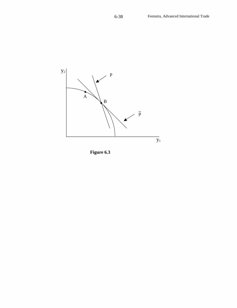
Feenstra, Advanced International Trade6-38
y2
y1
B
Figure 6.3
p~
p
A
Feenstra, Advanced International Trade6-39
Total profits earned by firms in the autarky equilibrium are v'wy'p aaa − , and each
consumer is entitled to some fixed fraction hλ of these. Then the autarky budget constraint of
consumer h is re-written from (6.1) as:
h'aha'a vwcp ≤ + )v'wy'p( aaah −λ , (6.15)
where hv is the vector of fixed factor supplies from individual h. Let us now open the
economy to trade at the prices p, and introduce a system of lump-sum transfers, so the post-trade
budget constraint of each consumer is:
hhh Rv'wc'p +≤ + )v'wy'p(h −λ , (6.16)
and the lump-sum transfers to each individual are:
hahaah v)'ww(c)'pp(R −−−= + )v'wy'p( aaah −λ )v'wy'p(h −λ− . (6.17)
It is straightforward to show that these transfers will allow each individual to obtain at least their
autarky consumption bundle, so that they are no worse off. The question, then, is whether the
government can afford this policy.
Summing the transfers in (6.17), and reversing the sign, we obtain:
∑∑∑===
−−−=−H
1h
haH
1h
haaH
1h
h v)'ww(c)'pp(R )v'wy'p[( aaaH
1h
h −λ− ∑=
)]v'wy'p( −−
v)'ww(y)'pp( aaa −−−= )v'wy'p( aaa −− + )v'wy'p( −
)y'py'p( a−≥ , (6.18)
where the second line follows by using aH1h
ha yc =∑ = , vvH1h
h =∑ = and 1H1h
h =λ∑ = , and the
third line follows by canceling terms.
Feenstra, Advanced International Trade6-40
If condition (6.18) is non-negative, this sufficient to ensure Pareto gains can be achieved.
That condition is readily interpreted as saying that the value of GDP evaluated at free trade
prices should not fall. In Figure 6.3, this means that the autarky equilibrium needs to lie to the
left of point B, such as at point A. Recalling the industry 1 is imperfectly competitive, this
condition ensures the Pareto gains that the output of the imperfectly competitive industry
increases. While this condition ensures that the value of GDP increases in Figure 6.3, let us see
whether this it ensures Pareto gains more generally.
Consider the following condition to guarantee Pareto gains, as proposed by Helpman
(1984, p. 353):
0)yy()'p~p( a ≥−− , (6.19)
where p~ are the marginal revenue/prices under free trade. For competitive industries with
ii p~p = , condition (6.19) is automatically satisfied, while for imperfectly competitive industries
with ii p~p > , (6.19) will be satisfied if aii yy ≥ so their outputs do not fall going from autarky to
free trade. When (6.19) holds, then we have:
0)yy('p~)yy('p aa ≥−≥− , (6.20)
where the last inequality holds because the value of “shadow GDP” y'p~)y,p~(G = is maximized
at the equilibrium outputs y. Thus, (6.19) implies that (6.20) holds, which ensures that (6.18) is
also non-negative. We have therefore proved:
Feenstra, Advanced International Trade6-41
Theorem (Markusen, 1981; Helpman, 1984)
With constant returns to scale, if the output of every good produced under imperfect competition
does not fall going from autarky to free trade, then Pareto gains from trade can be achieved using
the lump-sum transfers in (6.17).
Thus, the key condition to achieve Pareto gains is that industry output does not fall in the
imperfectly competitive industries of the country in question. Admittedly, it may be hard to
achieve this condition across several countries: if industry output increases in one country, is it
not more likely to fall in another? This was the case analyzed by Markusen (1981). For two
countries that are identical except for size, he found that the smaller country would experience an
increase in the good sold under imperfect competition, but not the larger country. This means
that gains from trade are assured only for the smaller country.
One way to deal with this problem of “unequal” gains across country is to derive a
condition for Pareto gains due to free trade among a group of countries i=1,…,C (which can be
the entire world). As we found for the analysis of customs unions in the previous section, we
will end up summing the criterion in (6.18) across the group of countries. That is, the combined
government budget for the group is non-negative provided that the terms of trade with respect to
outside countries do not change, and:
0)yy('p iaiC
1i≥−∑
=. (6.18’)
How can we ensure that (6.18’) holds? Consider the generalization of the Helpman
(1984b) condition in (6.19):
Feenstra, Advanced International Trade6-42
0)yy()'p~p( iaiiC
1i≥−−∑
=, (6.19’)
where ip~ are the marginal revenue/prices under free trade. These will be identical across
countries in the competitive industries, but in general can differ across countries in the non-
competitive industries. A sufficient condition to rule this out, however, is to have marginal costs
equal across countries, due to identical technologies and factor price equalization. In that case,
we can write p~p~i = in (6.19’).
When condition (6.19’) holds, we readily obtain,
0)yy(p~)yy('p iaiiC
1i
iaiC
1i≥−≥− ∑∑
==, (6.20’)
where the last inequality holds because iaiii y'p~y'p~ ≥ for every country of the union. We
therefore see that (6.19’) implies (6.18’), which guarantee Pareto gains for the group of
countries. If marginal costs are identical across countries in the free trade equilibrium, so
p~p~i = , then condition (6.19’) will be satisfied whenever the total group output of each
imperfectly competitive good does not fall. This condition generalizes the above theorem, and
ensures Pareto gains for the group of countries, though there will still be a need to transfer
income between them as we have discussed in the previous section for customs unions.
Let us now consider the case of monopolistic competition and increasing returns to scale.
In that case, each firm is producing a differentiated product. As discussed by Helpman and
Krugman (1985, chap. 9), Pareto gains from trade are ensured if: (i) the output of each firm still
producing does not fall going from autarky to free trade; (ii) total industry output (equal to the
number of firms times the output of each) does not fall going from autarky to free trade; (ii) the
set of goods available to consumers is not reduced due to the opening of trade. Notice that
Feenstra, Advanced International Trade6-43
condition (i) allows some firms to exit due to the opening of trade, as discussed in chapter 5.
Indeed, their departure gives room for other firms to increase their outputs and take advantage of
economies of scale. Examples can be constructed, however, where one or more of these
conditions are violated so that losses from trade are possible.8 The question is whether there are
some “reasonable” assumptions that rule this out.
Helpman and Krugman (1985, pp. 187-190) have identified quite weak assumptions to
ensure that conditions (i)-(iii) hold. Specifically, they assume that each industry in the economy
is organized like the Krugman model considered at the beginning of chapter 5, with consumption
in each industry coming from an additively separable sub-utility function. Assume that: (a) the
elasticity of demand in non-decreasing in output; (b) there is a constant share of expenditure
spent on each differentiated goods industry; (c) the production function for each differentiated
good is homothetic; (d) equilibria in each differentiated goods industry is symmetric, with
identical costs, prices and output. Then they demonstrate that the opening of trade will lead to at
least as many goods, and at least as much output of each provided only that the world output of
each differentiated goods industry does not contract. In that case, there is not even any need for
transfers between countries to ensure Pareto gains from trade.
Conclusions
The idea that countries gain from trade is as old as the idea of comparative advantage
itself – Ricardo wrote his model of trade between England and Portugal to demonstrate both
claims. But gains “for a country” does not have a well-defined meaning unless we specify what
this implies for the many different individuals located there. In this chapter we have taken the
heterogeneity of individuals seriously, and identified conditions under which all agents can gain
8 See Lawrence and Spiller (1983) and Francois and van Ypersele (2002).
Feenstra, Advanced International Trade6-44
from trade, i.e. Pareto gains are achieved. The lump sum transfers that we have discussed
require too much information to be implemented in practice, but are still valuable because they
allow us to show that Pareto gains are in principle possible. The commodity tax/subsidies
introduced by Dixit and Norman (1980) are an alternative means of achieving Pareto gains. In
the presence of mobility costs, however, these may need to be supplemented with some form of
trade adjustment assistance.
Our results for Pareto gains within a country can be extended to cover the comparison of
any two trading situations, and also to cover multiple countries, as with customs unions and free
trade areas. In addition, we showed how imperfect competition could be incorporated. Missing
from our analysis, however, is an important topic related to imperfect competition and the gains
from regional trade agreements. Suppose that trade in differentiated products occurs under
monopolistic competition, subject to “iceberg” transportation costs as discussed in chapter 5.
Furthermore, suppose that the countries forming a regional agreement do not aim to keep welfare
in the rest of world unchanged; on the contrary, these countries adjust the tariffs applied to the
rest of the world to their own optimal advantage. In the next chapter, we will call this the
“optimal” tariff, and it is applied to shift a country’s terms of trade in its favor. Finally, suppose
that the world splits up into a number of such regional areas, each of them equally sized. Then
how does the formation of these areas impact world welfare?
This question has been addressed by Krugman (1991a, 1991b), with two quite distinct
answers. First, ignoring transportation costs, Krugman (1991a) argues that with the world
divided into a number of equally-sized regional trading areas, the worst number of such areas is
three. The logic of this proposition is that with just one area, encompassing all countries, we
have the highest level of world welfare (i.e. global free trade). Conversely, with many equal-
Feenstra, Advanced International Trade6-45
sized areas, each group of countries will have little influence in changing their terms of trade, so
tariffs are low and we are again close to free trade. But at some intermediate number of areas,
tariffs will be higher and world welfare lower. Stylized calculations suggests that world welfare
is minimized with three areas, which is a depressing result in view of the possible formation of
three trading regions in reality: the Americas, Europe and Asia.
But this view of the world ignores the fact that actual trading regions are often between
geographically close countries (e.g. the EEC and NAFTA), so the “natural” trading advantages
of these countries are just enhanced by the regional agreement. To see how this affects the
argument, suppose now that there are three continents (America, Europe and Asia) with multiple
countries in each. As in Krugman (1991b), take an extreme case where transportation costs are
infinite for trade between the continents, but zero within each continent. In the absence of any
regional agreements, the countries in each continent will be applying optimal tariffs against each
other. But with a regional free trade agreement on each continent, then tariffs are eliminated,
and world welfare would be maximized: the fact that outside countries are excluded from each
regional agreement is irrelevant, since transportation costs between the continents are so high.
So in this case, three regional trading areas maximize world welfare!
These two starkly different results suggest that the pattern and level of transportation
costs between countries is crucial to determining the welfare effects of regional agreements.
Obviously, we need to go beyond the two extreme cases of Krugman (1991a,b), and this is done
by Frankel (1997). Continuing with Krugman’s example of a world divided into continents, each
of which is divided into multiple countries, Frankel explores the welfare impact of regional
agreements within or across continents. An agreement within a continent (where transportation
costs are low) is called “natural,” while an agreement across continents (where transportation
Feenstra, Advanced International Trade6-46
costs are high) is called “unnatural.” Frankel confirms that “natural” trading areas are more
likely to lead to world welfare gains than “unnatural” areas.9 However, it turns out that having
regional agreements within continents is not always welfare improving, and the case where these
“natural” areas fail to lead to world gains is called “supernatural.” This brief summary is meant
to suggest that the impact of regional trade agreements – in theory or in practice – is still a wide
open area for research, and we shall return to this topic in chapter 9.
9 In a test of this proposition, Krishna (2002) provides empirical evidence that raises doubts on the link between“natural” trading areas (between close countries) and welfare gains.
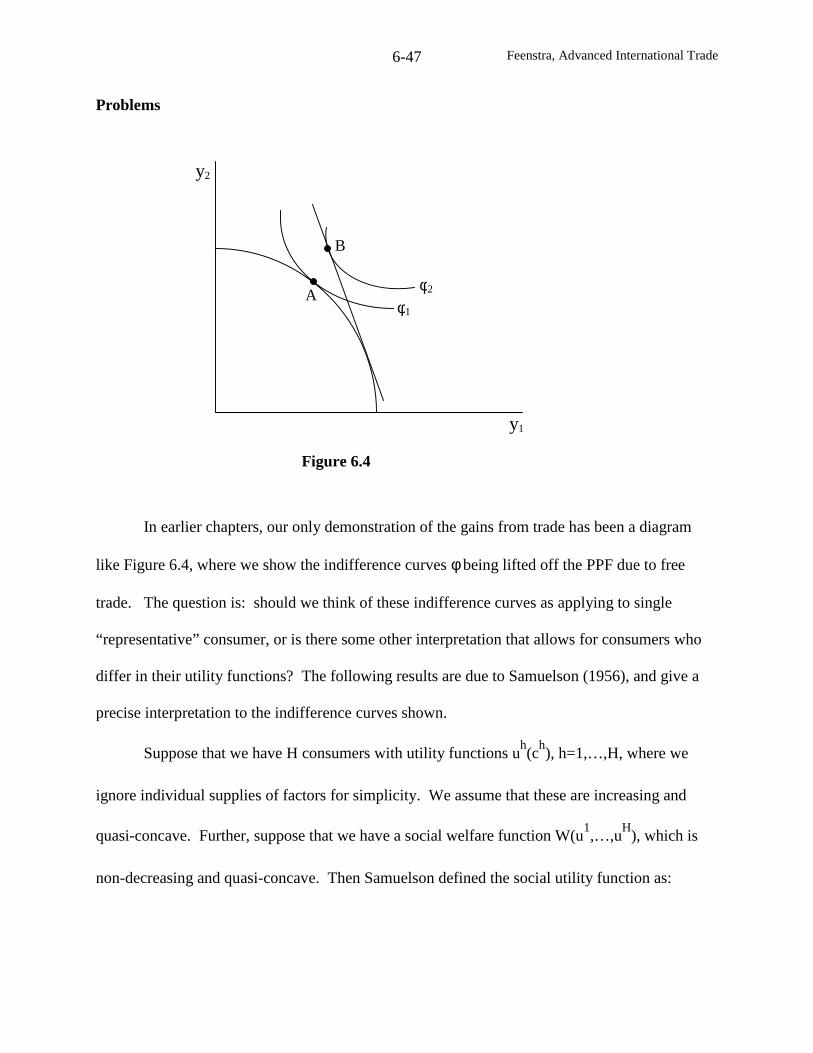
Feenstra, Advanced International Trade6-47
Problems
In earlier chapters, our only demonstration of the gains from trade has been a diagram
like Figure 6.4, where we show the indifference curves φbeing lifted off the PPF due to free
trade. The question is: should we think of these indifference curves as applying to single
“representative” consumer, or is there some other interpretation that allows for consumers who
differ in their utility functions? The following results are due to Samuelson (1956), and give a
precise interpretation to the indifference curves shown.
Suppose that we have H consumers with utility functions uh(c
h), h=1,…,H, where we
ignore individual supplies of factors for simplicity. We assume that these are increasing and
quasi-concave. Further, suppose that we have a social welfare function W(u1,…,u
H), which is
non-decreasing and quasi-concave. Then Samuelson defined the social utility function as:
B
A
y2
φ1
φ2
y1
Figure 6.4
Feenstra, Advanced International Trade6-48
∑=≥
≤=φH
1h
hHH11
0ccc.st)]c(u,),c(u[Wmax)c(
hL . (6.21)
Thus, this social utility function takes the total amount of consumption goods available, c, and
allocates it across individuals so as to maximize social welfare. This allocation is a form of
“lump sum” transfers, where we are physically allocating the goods (though the outcome would
be similar if we used lump sum transfers of income instead).
Samuelson argued that we could think of the indifference curves in Figure 6.4 as being
iso-curves of the function φ, so moving to a higher indifference curve due to trade (as illustrated)
means that social welfare has indeed increased.
To further understand Samuelson’s approach, answer the following:
6.1 The fact that we are moving from a welfare level of φ1 in Figure 6.4 to φ2 due to the opening
of trade proves that some person(s) utility must have increased, but it does not prove that
everyone’s utility has increased. Can you think of a special form for the welfare function W
that will ensure that when φgoes up, then everyone’s utility must go up as well? [This social
welfare function is used by Chipman (1987, p. 528), for example.]
Feenstra, Advanced International Trade
Chapter 7: Import Tariffs and Dumping
There are various reasons why countries use import tariffs and other types of trade
policies. Nearly all countries have used these instruments in early stages of their development to
foster the growth of domestic industries, in what is called import substitution. Such policies
have been heavily criticized for protecting inefficient domestic industries from international
competition. Many countries have later switched to an export promotion regime, under which
industries are expected to meet international competition through exports, albeit with subsidies
(hopefully temporary) given to exporters. The more than 140 members of the WTO have all
committed to abandon such heavily regulated trade regimes, and move towards substantially
freer trade. One question, then, is whether the use of import tariffs and other trade policies at
early stages of the development process has any rationale at all, especially when other markets
(such as for capital) might not be functioning well. While this is too big a question to deal with
adequately in this chapter, we will briefly discuss the rationale for temporary tariffs in what is
called “infant industry” protection.
A second question concerns the welfare cost of tariffs and quotas in situations where
other markets are working well. Even under the GATT/WTO, countries are permitted to apply
tariffs in a number of cases, including: (i) “escape clause” tariffs, under which countries
temporarily escape from their promise to keep tariffs low, due to injury in an import-competing
industry; (ii) antidumping duties, under which tariffs are applied to offset import prices that are
“too low.” For theoretical purposes, we can think of escape clause tariffs as exogenously
imposed on exporting firms, and this will be our assumption in the first part of the chapter. We
will examine the response of the exporters, as well as the response of import-competing firms, to
such tariffs. In particular, we are interested in whether there is any “strategic” role for trade
Feenstra, Advanced International Trade7-2
policy, whereby it gives an advantage to importing firms that leads to a welfare gain for the
importing country. This possibility is associated with the work of Brander and Spencer
(1984a,b). The response of firms to the tariff depends on the market structure, and we shall
investigate a series of cases, concluding with an empirical investigation of these tariffs as applied
to U.S. imports of compact trucks and heavyweight motorcycles (Feenstra, 1989).
Following this, we turn to a discussion of dumping. We suggest that this phenomena can
be viewed as a natural attempt of imperfectly competitive firms to enter each others markets, as
in the “reciprocal dumping” model of Brander (1981) and Brander and Krugman (1983). As
such, it is likely to bring gains to consumers through lower prices. These gains will be offset by
the use of anti-dumping duties, especially since these duties must be treated as endogenous:
their application will depend on the prices charged by the exporting firms. Exporting firms will
have an incentive to raise their prices even if there is only a threat of antidumping duties being
imposed, and to raise them even further if the duties are actually imposed. For these reasons,
consumer and social losses due to antidumping actions are particularly high. We review
empirical work by Prusa (1991, 1992), Staiger and Wolak (1996) and Blonigen and Haynes
(2002), who estimate the price and quantity effects of antidumping actions.
Tariffs under the GATT/WTO
For member countries of the WTO the use of tariffs or quotas is allowed under some
circumstances. For example, Article XIX of the GATT (see Table 6.1), called the “escape
clause,” allows for the temporary use of protection when domestic industries are experiencing
unusual import competition. In order for the articles of GATT to have legal standing in its
member countries, they must be reflected in a set of trade laws within each country. In the
Feenstra, Advanced International Trade7-3
United States, Article XIX was incorporated into Title II, Section 201 of the Trade Act of 1974,
which states in part that:
Title II, RELIEF FROM INJURY CAUSED BY IMPORT COMPETITION
Section 201. INVESTIGATION BY INTERNATIONAL TRADE COMMISSION
(a) (1) A petition for eligibility for import relief for the purpose of facilitating orderly
adjustment to import competition may be filed with the International Trade Commission
… by an entity, including a trade association, firm, certified or recognized union, or a
group of workers, which is representative of the industry…
(b) (1) … upon the filing of a petition under subsection (a) (1), the Commission shall
promptly make an investigation to determine whether an article is being imported into the
United States in such increased quantities as to be a substantial cause of serious injury, or
threat thereof, to the domestic industry producing an article like or directly competitive
with the imported article…
(4) For the purposes of this section, the term “substantial cause” means a cause which
is important and not less than any other cause.
Source: U.S. Public Law 93-618, Jan. 3, 1975
It can be seen that in order to qualify for tariffs protection under Section 201, several
criterion need to be met, the most important of which is that imports must be a “substantial cause
of serious injury, or threat thereof, to the domestic industry,” where a “substantial cause” must be
“not less than any other cause.” This legal language is very important in practice: it means that
a tariff will be granted only if rising imports are the most important cause of injury to the
domestic industry. This criterion is difficult enough to establish that escape clause protection is
used infrequently. This is shown in Table 7.1, taken from Hansen and Prusa (1995). Over the
years 1980-1988, there were only 19 escape clause case files in the United States, of which
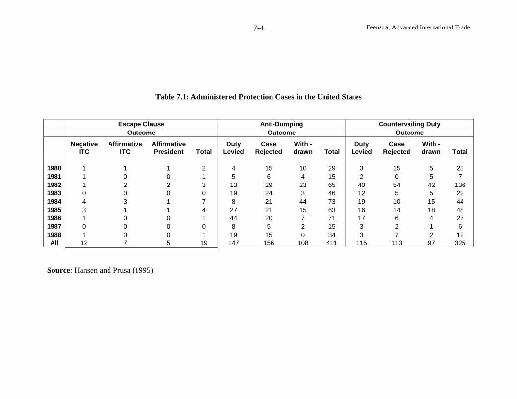
Feenstra, Advanced International Trade7-4
Table 7.1: Administered Protection Cases in the United States
Escape Clause Anti-Dumping Countervailing DutyOutcome Outcome Outcome
NegativeITC
AffirmativeITC
AffirmativePresident Total
DutyLevied
CaseRejected
With -drawn Total
DutyLevied
CaseRejected
With -drawn Total
1980 1 1 1 2 4 15 10 29 3 15 5 231981 1 0 0 1 5 6 4 15 2 0 5 71982 1 2 2 3 13 29 23 65 40 54 42 1361983 0 0 0 0 19 24 3 46 12 5 5 221984 4 3 1 7 8 21 44 73 19 10 15 441985 3 1 1 4 27 21 15 63 16 14 18 481986 1 0 0 1 44 20 7 71 17 6 4 271987 0 0 0 0 8 5 2 15 3 2 1 61988 1 0 0 1 19 15 0 34 3 7 2 12All 12 7 5 19 147 156 108 411 115 113 97 325
Source: Hansen and Prusa (1995)
Feenstra, Advanced International Trade7-5
12 obtained a negative recommendation from the U.S. International Trade Commission (ITC).
The remaining seven affirmative cases went to the President for a final ruling, and he gave a
positive recommendation for import protection in only five cases, or less than one per year. We
will investigate two of these U.S. cases in this chapter, one of which (heavyweight motorcycles)
received import protection under Section 201, and the other of which (compact trucks) was
denied under Section 201 but was able to get tariff protection by other means.
As an alternative to the escape clause, firms can file for import protection under the anti-
dumping provision of the WTO, which is Article VI (see Table 6.1). This provision has been
incorporated into Title VII of U.S. trade laws, where Section 303 deals with “countervailing
duties” and Section 731 deals with “antidumping duties.” Countervailing duties are applied to
offset foreign subsidies that lower the price of the foreign export good in the home market.
Antidumping deals with cases where it is believed that a foreign firm is selling goods in the
home (i.e. importing) market at either a lower price than in its own market, or if there is no
foreign price to observe, then at less than its average costs of production. The cases filed in the
United States under each of these provisions are also shown in Table 7.1, and it can be seen that
the number of these vastly exceeds escape clause cases.
Over 1980-1988, there were more than 400 antidumping cases files in the U.S., and of
these, about 150 were rejected and another 150 had duties levied. In order to have duties applies,
a case must first go to the Department of Commerce (DOC), which rules on whether imports
have occurred as “less than fair value,” i.e. below the price or average costs in its own market.
These rulings were positive in 94% of cases during this period (Hansen and Prusa, 1995, p. 300).
The case is then brought before the ITC, which must rule on whether imports have caused
“material injury” to the domestic industry (defined as “harm that is not inconsequential,
Feenstra, Advanced International Trade7-6
immaterial, or unimportant”). This criterion is much easier to meet than the “substantial cause of
serious injury” provision of Section 201, and as a result, the ITC more frequently rules in favor
of antidumping duties. Furthermore, the application of duties does not require the additional
approval of the President. These legal factors explain the much greater use of antidumping than
the escape clause in the United States, and it is also becoming more commonly used in other
countries, as described by Prusa (2001).
There is a surprising third category of antidumping cases shown in Table 7.1: of the
roughly 400 cases in the U.S. over this period, about 100 or one-quarter of these were withdrawn
prior to a ruling by the ITC. What are we to make of these cases? Prusa (1991, 1992) describes
how U.S. antidumping law actually permits the U.S. firms to withdraw its case, and then acting
through an intermediary at the DOC, agree with the foreign firm on the level of prices and
market shares! This type of communication between two American firms would be illegal under
U.S. anti-trust law, of course, but is exempted from prosecution in anti-dumping cases under the
so-called Noerr-Pennington doctrine. As we would expect, these withdrawn cases result in a
significant increase in market prices, with losses for consumers, as will be discussed at the end of
the chapter.
Social Welfare
In the previous chapter we were careful to allow for heterogeneous consumers, and
considered systems of lump-sum transfers or commodity taxes and subsidies such that everyone
could be better off (Pareto gains from trade). It will now be convenient to adopt a simpler
measure of overall social welfare, without worrying about whether every individual is better off
or not. To construct this we need to have a method to “add up” the utilities of consumers. This
will be achieved by assuming that every individual has a quasi-linear utility function, given by
Feenstra, Advanced International Trade7-7
)c(Uc hhh0 + , where h
0c is the consumption of a numeraire good, and ch
is the consumption
vector of all other goods for consumer h=1,…,H, with Uh
increasing and strictly concave. Each
consumer maximizes utility subject to the budget constraint hhh0 Ic'pc ≤+ .
Let ch
= dh(p) denote the optimal vector of consumption for each individual, with
remaining income spent on the numeraire good, )p(d'pIc hhh0 −= . Then we can define social
welfare as the sum of individual utilities,
)]p(d[U)p(d'pI)I,p(W hhhhH
1h
+−≡∑=
, (7.1)
where total income is ∑ == H1h
h .II Notice that the sum over individuals of the last two terms on
the right of (7.1) gives consumer surplus. By the envelope theorem, the derivative of (7.1) is the
negative of total consumption, ∑ = −≡−=∂∂ H1h
h ).p(d)p(dp/W Thus, we can use the social
welfare function just like an indirect utility function for the economy as a whole.
Let us further simplify the analysis by supposing that there is only a single import good
subject to a tariff. Holding the prices of all other goods fixed, we will therefore treat p as a
scalar, denoting the price of that good in the importing country. Its world price is denoted by the
scalar p*, and the difference between these is the specific import tariff t, so p = p* + t. We
suppose that the numeraire good is also traded, at a fixed world price of unity. Labor is assumed
to be the only factor of production, and each unit of the numeraire good requires one unit of
labor. It follows that wages in the economy are also unity, so that total income equals the fixed
labor supply of L. These assumptions allow the economy to mimic a partial-equilibrium setting,
where wages are fixed and trade is balanced through flows of the numeraire good.
Feenstra, Advanced International Trade7-8
Output of the good in question is denoted by the scalar y, which may be produced by
competitive or imperfectly competitive firms. We suppose that the industry costs of producing
the good are denoted by C(y), with marginal costs )y('C .1 Imports are denoted by the scalar m =
d(p) – y, where 0)p('d < from the assumption that Uh
is strictly concave for all h. We assume
that revenue raised from the tariff, tm, is redistributed back to consumers, who are also each
entitled to profits from the import-competing industry, which are py – C(y). It follows that social
welfare is written as,
).t(W)]y(CpytmL,p[W ≡−++ (7.2)
This general expression for social welfare holds under perfect or imperfect competition.
In the former case, it is common to refer to profits [py – C(y)] as producer surplus, i.e. the return
to fixed factors of production in the industry. In the latter case, we denote profits of the domestic
industry by π= py – C(y), and will need to specify how these depend on actions of foreign firms.
We will be considering three cases: (i) perfect competition in the home and foreign industries;
(ii) foreign monopoly, with no domestic import-competing firms; (iii) duopoly, with one home
firm and one foreign firm engaged in either Cournot or Bertrand competition. A fourth case of
monopolistic competition is discussed by Helpman (1990), and is not covered here. We begin
with perfect competition, where we distinguish a small importing country, meaning that the
world price p* is fixed even as the tariff varies, and a large country, whose tariff affects the
foreign price p*.
1 Under perfect competition C(y) denotes industry costs, and under monopoly it denotes the firm’s costs. Underoligopoly with a homogeneous product, we should replace C(y) with NC(y), where N is the number of firms andC(y) is the costs of each. Similarly, we replace sales py in (7.2) by Npy. With free entry and zero profits, we cansimply omit the profit term in (7.2) and this amended welfare function still applies. The welfare function with adifferentiated import and domestic product will be described later in the chapter.
Feenstra, Advanced International Trade7-9
In each case, we are interested in how social welfare in (7.2) varies with the tariff. To
determine this, let us first derive a general expression for the change in welfare. Treating the
price p and output y as depending on the tariff, we can totally differentiate (7.2) to obtain:
.dt
dy)]y('Cp[
dt
*dpm
dt
dp
dp
dmt
dt
dy)]y('Cp[
dt
dp
dp
dmt
dt
dp1m
dt
dy)]y('Cp[
dt
dpy
dp
dmtm
dt
dp)p(d
dt
dW
−+−=
−++
−=
−+
+++−=
(7.3)
The second line of (7.3) follows by noting that y – d(p) = m and combining terms, while the third
line follows because p = p* + t, so that [1-(dp/dt)] = –dp*/dt.
We will be discussing each of the terms on the last line of (7.3) throughout this chapter,
but note here the similarity between these terms and those derived in the previous chapter. The
first term on the last line of (7.3) can be interpreted as the efficiency cost of the tariff, much like
the term )mm('t 011 − in chapter 6; the second term is the effect of the tariff on the foreign price
p*, or the terms of trade effect, like 010 m)'*p*p( − in chapter 6; and the third term reflects the
change in industry output times the price-cost margin, like )yy()'p~p( a−− in chapter 6. This
third term reflects the fact that with imperfect competition there is a gap between the price or
consumer valuation of a product, and the marginal costs to firms. This distortion due to
monopolistic pricing creates an efficiency loss, and any increase in domestic output will
therefore offset that loss and serve to raise welfare.
Feenstra, Advanced International Trade7-10
Perfect Competition, Small Country
Holding p* fixed, we already argued in the previous chapter that “free trade is better than
restricted trade for a small country.” In other words, the optimal tariff is zero. We now provide
a more direct demonstration of this result, and also show how the welfare loss due to a tariff can
be measured. Under perfect competition profits are maximized when )y('Cp = , so the final
term in (7.3) is zero. When world prices are fixed and domestic prices given by p = p* + t, then
dp*/dt = 0 and dp/dt = 1. Using these various relations in (7.3), we readily obtain:
dp
dmt
dt
dW = . (7.4)
Evaluating this expression at a zero tariff, we have:
0dt
dW
0t
==
. (7.4’)
This proves that social welfare has a critical point at a zero tariff, but we still need to
determine whether this is a maximum or not. Differentiating (7.4) and evaluating at t = 0,
0dp
dm
dt
Wd
0t2
2
<==
, (7.5)
where this sign is obtained because )"C/1()p('ddp/dm −= , with 0)p('d < from concavity of the
utility functions and 0"C > from the second-order condition for profit maximization. This
proves that the critical point at t = 0 is a local maximum, and in fact, it is also a global maximum
since with 0dp/dm < then t = 0 is the only tariff at which (7.4) equals zero. Therefore, the
optimal tariff for a small country is zero.
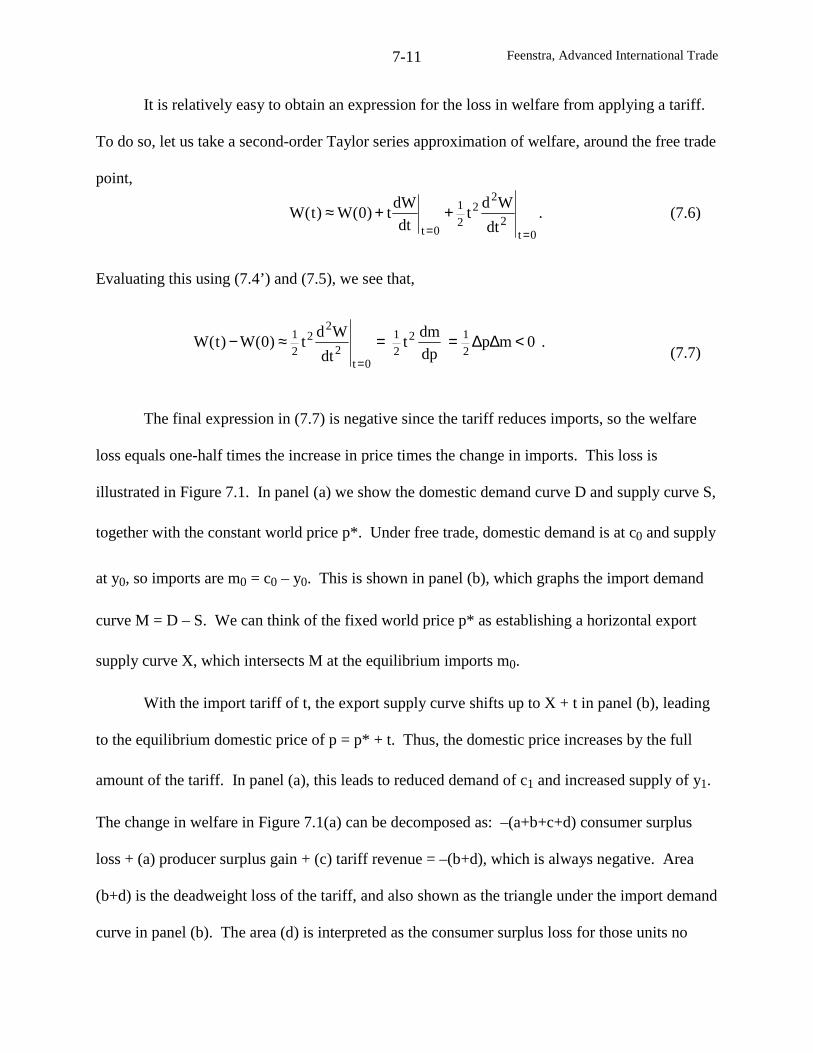
Feenstra, Advanced International Trade7-11
It is relatively easy to obtain an expression for the loss in welfare from applying a tariff.
To do so, let us take a second-order Taylor series approximation of welfare, around the free trade
point,
0t2
22
2
1
0t dt
Wdt
dt
dWt)0(W)t(W
==++≈ . (7.6)
Evaluating this using (7.4’) and (7.5), we see that,
.0mpdp
dmt
dt
Wdt)0(W)t(W
2
122
1
0t2
22
2
1 <∆∆==≈−=
(7.7)
The final expression in (7.7) is negative since the tariff reduces imports, so the welfare
loss equals one-half times the increase in price times the change in imports. This loss is
illustrated in Figure 7.1. In panel (a) we show the domestic demand curve D and supply curve S,
together with the constant world price p*. Under free trade, domestic demand is at c0 and supply
at y0, so imports are m0 = c0 – y0. This is shown in panel (b), which graphs the import demand
curve M = D – S. We can think of the fixed world price p* as establishing a horizontal export
supply curve X, which intersects M at the equilibrium imports m0.
With the import tariff of t, the export supply curve shifts up to X + t in panel (b), leading
to the equilibrium domestic price of p = p* + t. Thus, the domestic price increases by the full
amount of the tariff. In panel (a), this leads to reduced demand of c1 and increased supply of y1.
The change in welfare in Figure 7.1(a) can be decomposed as: –(a+b+c+d) consumer surplus
loss + (a) producer surplus gain + (c) tariff revenue = –(b+d), which is always negative. Area
(b+d) is the deadweight loss of the tariff, and also shown as the triangle under the import demand
curve in panel (b). The area (d) is interpreted as the consumer surplus loss for those units no
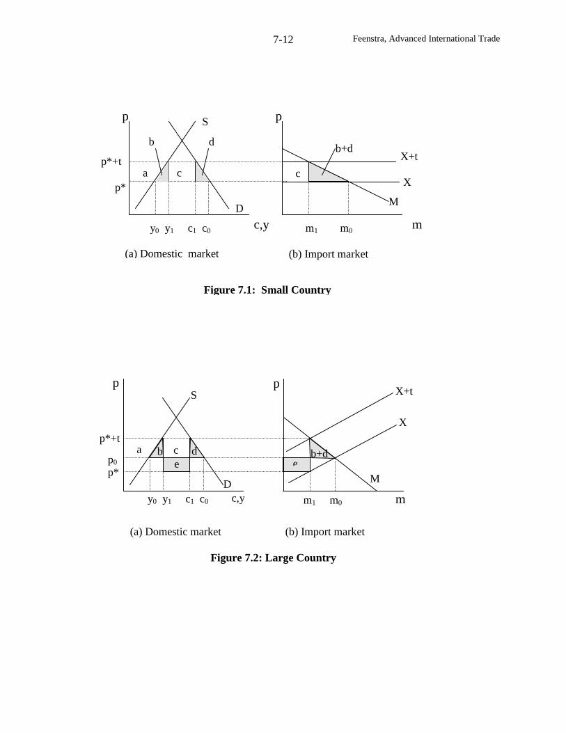
Feenstra, Advanced International Trade7-12
a c
p
a cp*+t
p0
p*
S
b d
p
m
e
Dc,yy0 y1 c1 c0 m1 m0
M
X+t
eb+d
(a) Domestic market (b) Import market
Figure 7.2: Large Country
D
p*+t
p*
p
c,y
S
y0 y1 c1 c0
(a) Domestic market
db
p
mm1 m0
(b) Import market
X+t
X
M
b+d
Figure 7.1: Small Country
c
X
Feenstra, Advanced International Trade7-13
longer purchased (i.e. c0–c1), while the area (b) is interpreted as the increase in marginal costs
(along the supply curve) for the extra units produced (i.e. y1–y0).
So we see that the deadweight loss of the tariff can be measured by a triangle under the
import demand curve. Since both the height and the base of the triangle depend on the tariff, the
area of the triangle itself is of the second-order of smalls for a small tariff, i.e. the deadweight
loss in (7.7) depends on the square of the tariff. Notice that we can re-write (7.7) to measure the
deadweight loss as a fraction of import expenditure:
.m
p
dp
dm
p
t
2
1
pm
)0(W)t(W2
≈−(7.7’)
For example, with a 10% tariff and an import demand elasticity of 2, the deadweight loss
relative to import expenditure will be 1%. As is typical for triangle calculations, we see that the
deadweight loss is quite small for moderate tariffs. This fact has led many researchers to
conclude that a formula like (7.7’) does not capture the inefficiencies present in import
substitution regimes. We will be investigating some reasons why the deadweight loss of trade
restrictions may well be greater than (7.7’). This can occur if foreign firms anticipate the tariffs,
as with antidumping duties (discussed later in this chapter), or if quotas are used instead of tariffs
(discussed in the next chapter), or due to the effect of tariffs on decreasing the variety of import
products available. This latter effect has been emphasized by Feenstra (1992) and Romer (1994).
Both authors provide simple formulas to compute welfare losses due to a reduction in import
varieties, and these are much greater than (7.7’). In addition, Feenstra (1988b) and Klenow and
Rodrígruez-Clare (1997) provide estimates of the welfare gain due to new import varieties,
which can be substantial.
Feenstra, Advanced International Trade7-14
Perfect Competition, Large country
For a large country, we suppose that the world price of imports depends on the tariff
chosen, which is written as p*(t). Generally, we define the terms of trade as the price of a
country’s exports divided by the price of its imports, so that a fall in the import price p* is an
improvement in the terms of trade. We will argue a tariff leads to such an improvement in the
terms of trade under perfect competition, as we assume in this section. In the next section we
will examine the sign of this derivative under foreign monopoly.
The domestic price of the import good is p = p* + t, so now dp*/dt ≠ 0 and dp/dt ≠ 1. We
still have )y('Cp = under perfect competition, so (7.3) becomes,
dt
*dpm
dt
dp
dp
dmt
dt
dW −= . (7.8)
The first term is interpreted as the marginal deadweight loss from the tariff; and the second term
is the terms of trade effect of the tariff, i.e. the reduction in the price of p* times the amount of
imports. The sign of dp*/dt can be determined from Figure 7.2. In panel (a), we show the
domestic demand curve D and supply curve S, which lead to the import demand curve M=D-S in
panel (b). Also shown is the foreign supply curve X, which we assume is upward sloping. The
initial equilibrium foreign and domestic price is *0p = p0. The tariff shift up the export supply
curve to X + t, which intersects import demand at the new domestic price p = p* + t. It is clear
from the diagram that the increase in the domestic price from p0 to p* + t is less than the amount
of the tariff t, which implies that the new foreign price p* is less than its initial value *0p . This is
a terms of trade gain for the importing country.
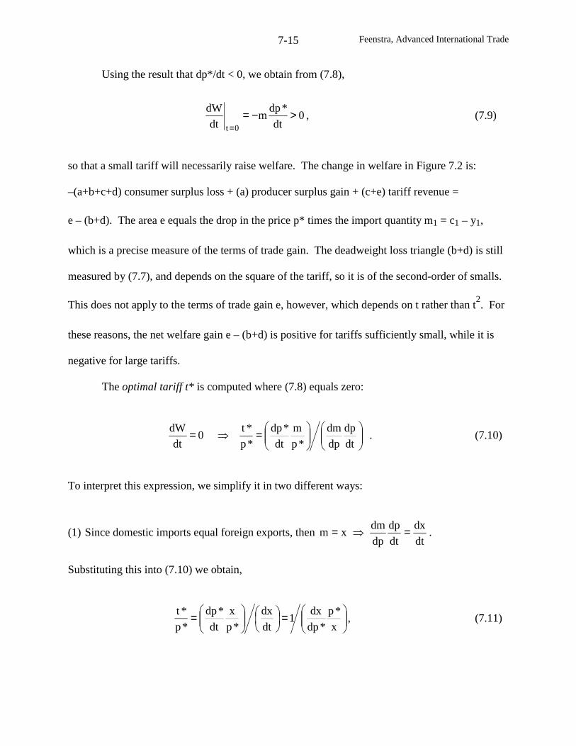
Feenstra, Advanced International Trade7-15
Using the result that dp*/dt < 0, we obtain from (7.8),
0dt
*dpm
dt
dW
0t
>−==
, (7.9)
so that a small tariff will necessarily raise welfare. The change in welfare in Figure 7.2 is:
–(a+b+c+d) consumer surplus loss + (a) producer surplus gain + (c+e) tariff revenue =
e – (b+d). The area e equals the drop in the price p* times the import quantity m1 = c1 – y1,
which is a precise measure of the terms of trade gain. The deadweight loss triangle (b+d) is still
measured by (7.7), and depends on the square of the tariff, so it is of the second-order of smalls.
This does not apply to the terms of trade gain e, however, which depends on t rather than t2. For
these reasons, the net welfare gain e – (b+d) is positive for tariffs sufficiently small, while it is
negative for large tariffs.
The optimal tariff t* is computed where (7.8) equals zero:
=⇒=dt
dp
dp
dm
*p
m
dt
*dp
*p
*t0
dt
dW. (7.10)
To interpret this expression, we simplify it in two different ways:
(1) Since domestic imports equal foreign exports, thendt
dx
dt
dp
dp
dmxm =⇒= .
Substituting this into (7.10) we obtain,
=
=x
*p
*dp
dx1
dt
dx
*p
x
dt
*dp
*p
*t, (7.11)
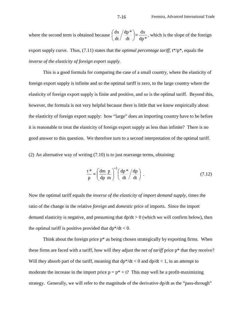
Feenstra, Advanced International Trade7-16
where the second term is obtained because*dp
dx
dt
*dp
dt
dx =
, which is the slope of the foreign
export supply curve. Thus, (7.11) states that the optimal percentage tariff, t*/p*, equals the
inverse of the elasticity of foreign export supply.
This is a good formula for comparing the case of a small country, where the elasticity of
foreign export supply is infinite and so the optimal tariff is zero, to the large country where the
elasticity of foreign export supply is finite and positive, and so is the optimal tariff. Beyond this,
however, the formula is not very helpful because there is little that we know empirically about
the elasticity of foreign export supply: how “large” does an importing country have to be before
it is reasonable to treat the elasticity of foreign export supply as less than infinite? There is no
good answer to this question. We therefore turn to a second interpretation of the optimal tariff.
(2) An alternative way of writing (7.10) is to just rearrange terms, obtaining:
=−
dt
dp
dt
*dp
m
p
dp
dm
p
*t1
. (7.12)
Now the optimal tariff equals the inverse of the elasticity of import demand supply, times the
ratio of the change in the relative foreign and domestic price of imports. Since the import
demand elasticity is negative, and presuming that dp/dt > 0 (which we will confirm below), then
the optimal tariff is positive provided that dp*/dt < 0.
Think about the foreign price p* as being chosen strategically by exporting firms. When
these firms are faced with a tariff, how will they adjust the net of tariff price p* that they receive?
Will they absorb part of the tariff, meaning that dp*/dt < 0 and dp/dt < 1, in an attempt to
moderate the increase in the import price p = p* + t? This may well be a profit-maximizing
strategy. Generally, we will refer to the magnitude of the derivative dp/dt as the “pass-through”
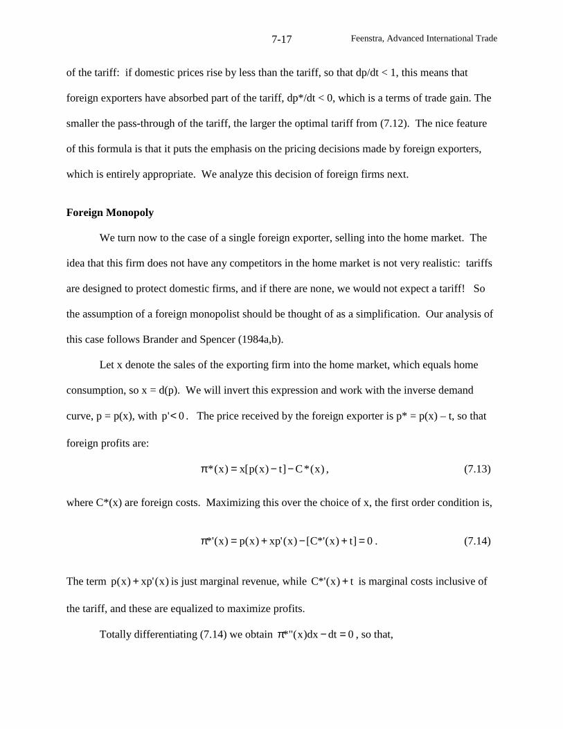
Feenstra, Advanced International Trade7-17
of the tariff: if domestic prices rise by less than the tariff, so that dp/dt < 1, this means that
foreign exporters have absorbed part of the tariff, dp*/dt < 0, which is a terms of trade gain. The
smaller the pass-through of the tariff, the larger the optimal tariff from (7.12). The nice feature
of this formula is that it puts the emphasis on the pricing decisions made by foreign exporters,
which is entirely appropriate. We analyze this decision of foreign firms next.
Foreign Monopoly
We turn now to the case of a single foreign exporter, selling into the home market. The
idea that this firm does not have any competitors in the home market is not very realistic: tariffs
are designed to protect domestic firms, and if there are none, we would not expect a tariff! So
the assumption of a foreign monopolist should be thought of as a simplification. Our analysis of
this case follows Brander and Spencer (1984a,b).
Let x denote the sales of the exporting firm into the home market, which equals home
consumption, so x = d(p). We will invert this expression and work with the inverse demand
curve, p = p(x), with 0'p < . The price received by the foreign exporter is p* = p(x) – t, so that
foreign profits are:
)x(*C]t)x(p[x)x(* −−=π , (7.13)
where C*(x) are foreign costs. Maximizing this over the choice of x, the first order condition is,
0]t)x(*'C[)x('xp)x(p)x(*' =+−+=π . (7.14)
The term )x('xp)x(p + is just marginal revenue, while t)x(*'C + is marginal costs inclusive of
the tariff, and these are equalized to maximize profits.
Totally differentiating (7.14) we obtain 0dtdx)x(*" =−π , so that,
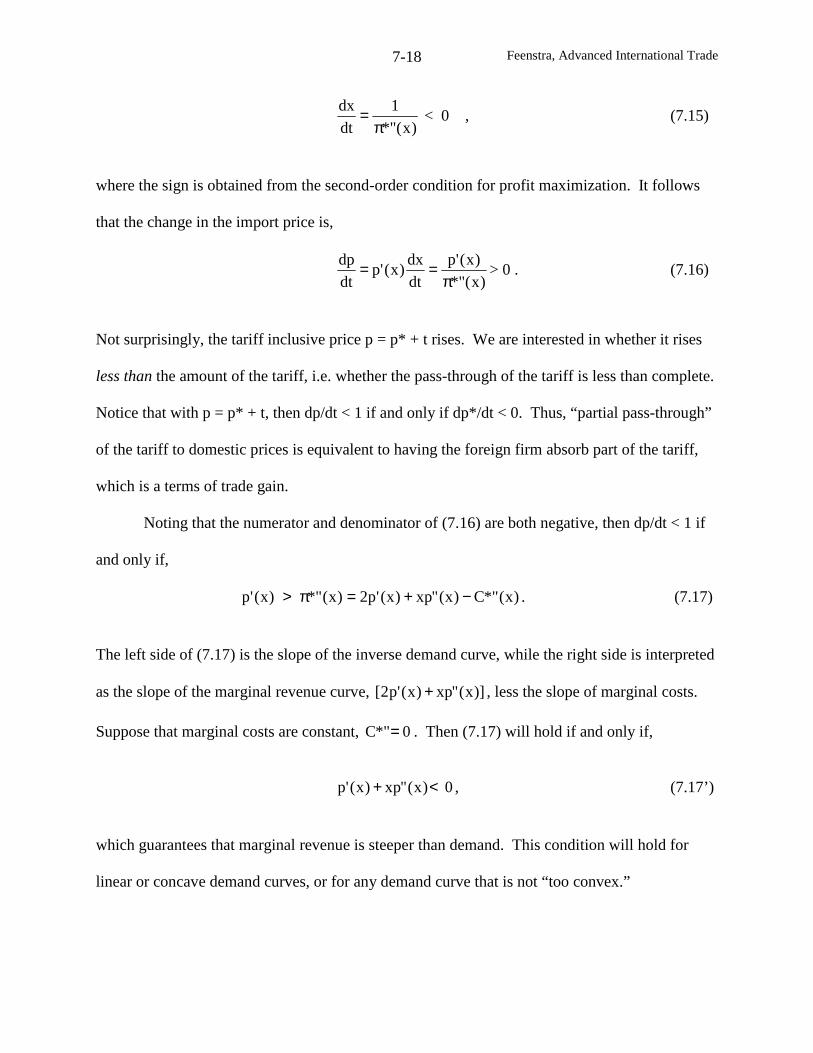
Feenstra, Advanced International Trade7-18
)x(*"
1
dt
dx
π= < 0 , (7.15)
where the sign is obtained from the second-order condition for profit maximization. It follows
that the change in the import price is,
)x(*"
)x('p
dt
dx)x('p
dt
dp
π== > 0 . (7.16)
Not surprisingly, the tariff inclusive price p = p* + t rises. We are interested in whether it rises
less than the amount of the tariff, i.e. whether the pass-through of the tariff is less than complete.
Notice that with p = p* + t, then dp/dt < 1 if and only if dp*/dt < 0. Thus, “partial pass-through”
of the tariff to domestic prices is equivalent to having the foreign firm absorb part of the tariff,
which is a terms of trade gain.
Noting that the numerator and denominator of (7.16) are both negative, then dp/dt < 1 if
and only if,
)x(*"C)x("xp)x('p2)x(*")x('p −+=π> . (7.17)
The left side of (7.17) is the slope of the inverse demand curve, while the right side is interpreted
as the slope of the marginal revenue curve, )]x("xp)x('p2[ + , less the slope of marginal costs.
Suppose that marginal costs are constant, 0*"C = . Then (7.17) will hold if and only if,
0)x("xp)x('p <+ , (7.17’)
which guarantees that marginal revenue is steeper than demand. This condition will hold for
linear or concave demand curves, or for any demand curve that is not “too convex.”
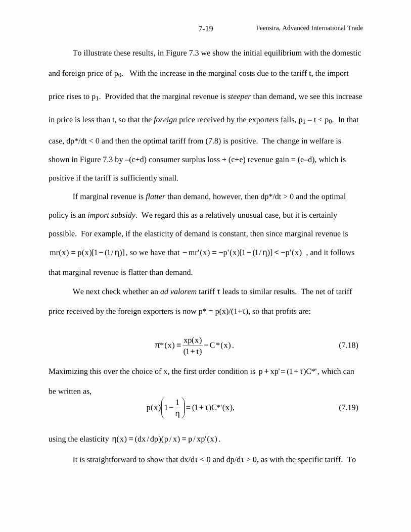
Feenstra, Advanced International Trade7-19
To illustrate these results, in Figure 7.3 we show the initial equilibrium with the domestic
and foreign price of p0. With the increase in the marginal costs due to the tariff t, the import
price rises to p1. Provided that the marginal revenue is steeper than demand, we see this increase
in price is less than t, so that the foreign price received by the exporters falls, p1 – t < p0. In that
case, dp*/dt < 0 and then the optimal tariff from (7.8) is positive. The change in welfare is
shown in Figure 7.3 by –(c+d) consumer surplus loss + (c+e) revenue gain = (e–d), which is
positive if the tariff is sufficiently small.
If marginal revenue is flatter than demand, however, then dp*/dt > 0 and the optimal
policy is an import subsidy. We regard this as a relatively unusual case, but it is certainly
possible. For example, if the elasticity of demand is constant, then since marginal revenue is
)]/1(1)[x(p)x(mr η−= , so we have that )x('p)]/1(1)[x('p)x('mr −<η−−=− , and it follows
that marginal revenue is flatter than demand.
We next check whether an ad valorem tariff τ leads to similar results. The net of tariff
price received by the foreign exporters is now p* = p(x)/(1+τ), so that profits are:
)x(*C)t1(
)x(xp)x(* −
+=π . (7.18)
Maximizing this over the choice of x, the first order condition is *'C)1('xpp τ+=+ , which can
be written as,
),x(*'C)1(1
1)x(p τ+=
η
− (7.19)
using the elasticity )x('xp/p)x/p)(dp/dx()x( ==η .
It is straightforward to show that dx/dτ < 0 and dp/dτ > 0, as with the specific tariff. To
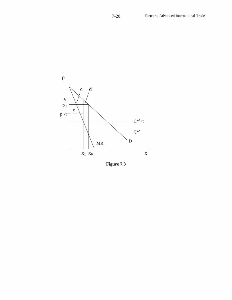
Feenstra, Advanced International Trade7-20
DMR
x1 x0 x
Figure 7.3
C*’+t
C*’
p
p1
p0
p1-te
c d
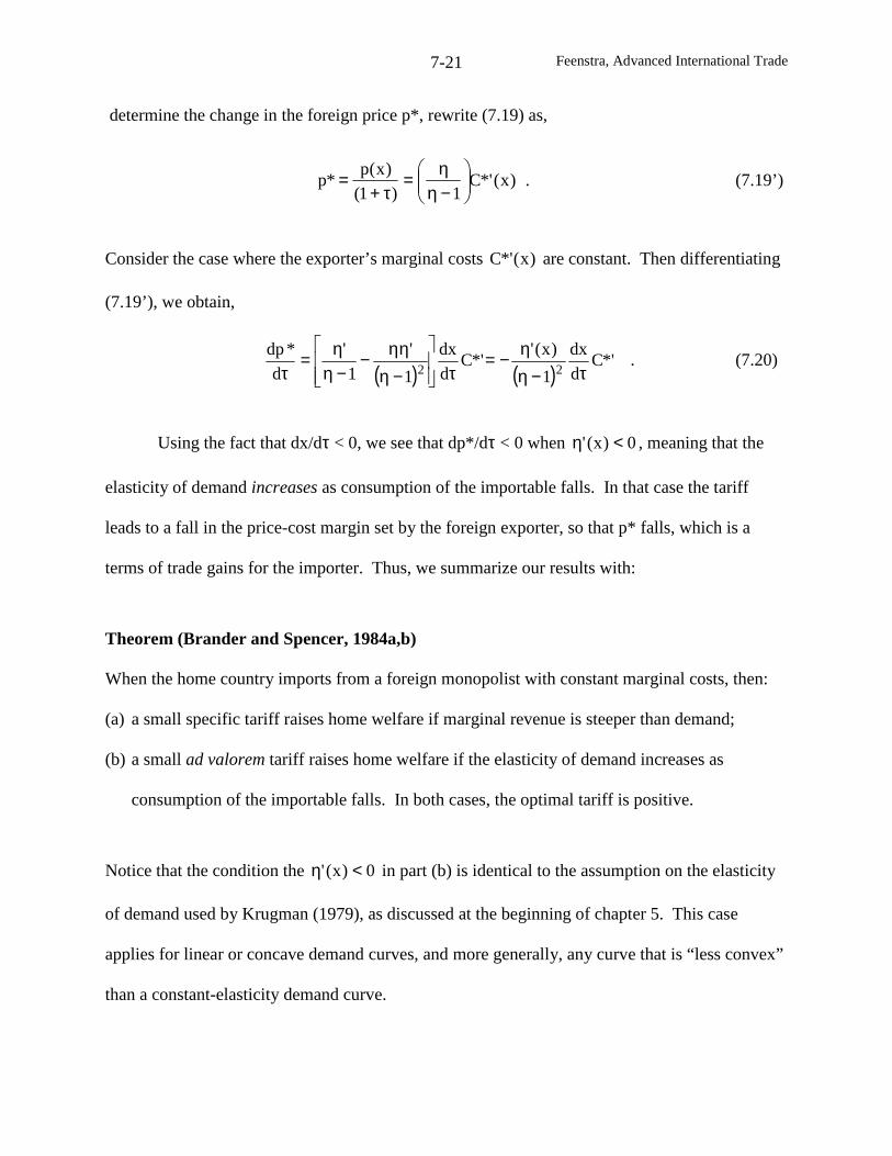
Feenstra, Advanced International Trade7-21
determine the change in the foreign price p*, rewrite (7.19) as,
)x(*'C1)1(
)x(p*p
−ηη=
τ+= . (7.19’)
Consider the case where the exporter’s marginal costs )x(*'C are constant. Then differentiating
(7.19’), we obtain,
( ) ( )*'C
d
dx
1
)x('*'C
d
dx
1
'
1
'
d
*dp22 τ−η
η−=τ
−ηηη−
−ηη=
τ. (7.20)
Using the fact that dx/dτ < 0, we see that dp*/dτ < 0 when 0)x(' <η , meaning that the
elasticity of demand increases as consumption of the importable falls. In that case the tariff
leads to a fall in the price-cost margin set by the foreign exporter, so that p* falls, which is a
terms of trade gains for the importer. Thus, we summarize our results with:
Theorem (Brander and Spencer, 1984a,b)
When the home country imports from a foreign monopolist with constant marginal costs, then:
(a) a small specific tariff raises home welfare if marginal revenue is steeper than demand;
(b) a small ad valorem tariff raises home welfare if the elasticity of demand increases as
consumption of the importable falls. In both cases, the optimal tariff is positive.
Notice that the condition the 0)x(' <η in part (b) is identical to the assumption on the elasticity
of demand used by Krugman (1979), as discussed at the beginning of chapter 5. This case
applies for linear or concave demand curves, and more generally, any curve that is “less convex”
than a constant-elasticity demand curve.
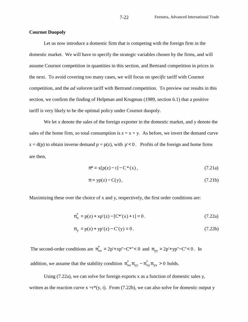
Feenstra, Advanced International Trade7-22
Cournot Duopoly
Let us now introduce a domestic firm that is competing with the foreign firm in the
domestic market. We will have to specify the strategic variables chosen by the firms, and will
assume Cournot competition in quantities in this section, and Bertrand competition in prices in
the next. To avoid covering too many cases, we will focus on specific tariff with Cournot
competition, and the ad valorem tariff with Bertrand competition. To preview our results in this
section, we confirm the finding of Helpman and Krugman (1989, section 6.1) that a positive
tariff is very likely to be the optimal policy under Cournot duopoly.
We let x denote the sales of the foreign exporter in the domestic market, and y denote the
sales of the home firm, so total consumption is z = x + y. As before, we invert the demand curve
z = d(p) to obtain inverse demand p = p(z), with 0'p < . Profits of the foreign and home firms
are then,
)x(*C]t)z(p[x* −−=π , (7.21a)
)y(C)z(yp −=π , (7.21b)
Maximizing these over the choice of x and y, respectively, the first order conditions are:
0]t)x(*'C[)z('xp)z(p*x =+−+=π . (7.22a)
0)y('C)z('yp)z(py =−+=π . (7.22b)
The second-order conditions are 0*"C"xp'p2*xx <−+=π and 0"C"yp'p2yy <−+=π . In
addition, we assume that the stability condition 0yx*xyyy
*xx >ππ−ππ holds.
Using (7.22a), we can solve for foreign exports x as a function of domestic sales y,
written as the reaction curve x =r*(y, t). From (7.22b), we can also solve for domestic output y
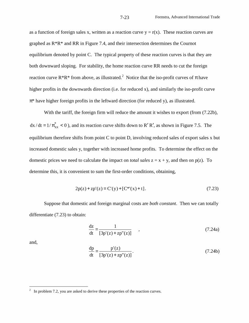
Feenstra, Advanced International Trade7-23
as a function of foreign sales x, written as a reaction curve y = r(x). These reaction curves are
graphed as R*R* and RR in Figure 7.4, and their intersection determines the Cournot
equilibrium denoted by point C. The typical property of these reaction curves is that they are
both downward sloping. For stability, the home reaction curve RR needs to cut the foreign
reaction curve R*R* from above, as illustrated.2 Notice that the iso-profit curves of πhave
higher profits in the downwards direction (i.e. for reduced x), and similarly the iso-profit curve
π* have higher foreign profits in the leftward direction (for reduced y), as illustrated.
With the tariff, the foreign firm will reduce the amount it wishes to export (from (7.22b),
0/1dt/dx *xx <π= ), and its reaction curve shifts down to R’ R’, as shown in Figure 7.5. The
equilibrium therefore shifts from point C to point D, involving reduced sales of export sales x but
increased domestic sales y, together with increased home profits. To determine the effect on the
domestic prices we need to calculate the impact on total sales z = x + y, and then on p(z). To
determine this, it is convenient to sum the first-order conditions, obtaining,
]t)x(*'C[)y('C)z('zp)z(p2 ++=+ . (7.23)
Suppose that domestic and foreign marginal costs are both constant. Then we can totally
differentiate (7.23) to obtain:
)]z("zp)z('p3[
1
dt
dz
+= , (7.24a)
and,
)]z("zp)z('p3[
)z('p
dt
dp
+= . (7.24b)
2 In problem 7.2, you are asked to derive these properties of the reaction curves.
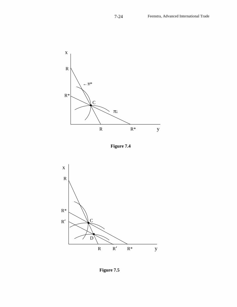
Feenstra, Advanced International Trade7-24
x
R
R*
←π*
π↓
R R* y
Figure 7.4
D
C
R R’ R* y
x
R
R*
R’
Figure 7.5
C
Feenstra, Advanced International Trade7-25
From (7.24a) we see that imports fall due to the tariff if 0)z("zp)z('p3 <+ . In that case the
numerator and denominator of (7.24b) are both negative, so that dp/dt < 1 if,
0)z("zp)z('p2)z("zp)z('p3)z('p <+⇔+> . (7.25)
The condition on the right of (7.25) states that marginal revenue for the market as a
whole, which is )z('zp)z(p + , slopes down. This is a significantly weaker condition than
(7.17’), which involved a comparison of the slopes of marginal revenue and demand; now, we
only need to check the slope of marginal revenue, and most demand curves will satisfy (7.25).
This includes the constant elasticity curve, for which 0)]/1(1)[z('p)z('mr <η−= . When (7.25)
is satisfied, then dz/dt < 0 in (7.24) and dp/dt < 1 in (7.24a), so there is a beneficial terms of trade
impact (dp*/dt < 0) for the importing country.
Checking social welfare, we again use the general change in social welfare in (7.3),
rewritten here using foreign exports (x) rather than home imports (m):
dt
dy)]y('Cp[
dt
*dpx
dt
dxt
dt
dW −+−= , (7.3’)
where the final term reflects the change in domestic output from equilibrium point C to point D.
The first term on the right of (7.3) vanishes for small tariffs, and the second term is positive
when (7.25) holds, so that a positive tariff improves the terms of trade. For the third term, in the
typical case where both reaction curves are downward sloping, with the home curve cutting the
foreign curve from above as shown in Figure 7.5, then we will have dy/dt > 0: the tariff will lead
to an increase in domestic output, which brings an additional terms of trade gain. In this case,
the optimal tariff is unambiguously positive.
Feenstra, Advanced International Trade7-26
However, the typical pattern of the reaction curves shown in Figure 7.5 need not hold,
and it is possible that the home curve slope upwards instead, in which case dy/dt < 0, so the tariff
reduces home output. This will tend to offset the terms of trade gains due to the tariff. With
constant marginal costs, it can be shown that this case is avoided, so that dy/dt > 0, provided that
0)z("yp)z('p <+ .3 This condition states that “perceived” marginal revenue for the foreign firm,
)z('yp)z(p + , is steeper than the demand curve p(z), and is somewhat weaker than (7.17’).
Combined with our finding that dp/dt < 1 when (7.25) holds, so that dp*/dt < 0, we therefore
have two distinct reasons why a tariff will raise social welfare: the terms of trade effect; and the
efficiency effect, whereby the tariff moves the home firm to a higher level of output at point D
and offsets the distortion between price and marginal cost.
The idea that imperfect competition might justify the “strategic” use of trade policy was
an area of very active research during the 1980s. In the tariff case we are discussing, it is
tempting to refer to the last term in (7.3) as a “profit shifting” motive for the use of tariffs,
suggesting that a “strategic” use of tariffs is to shift profits towards the home firm. But this
terminology must be interpreted with caution. There is no direct relation between the sign of the
last term in (7.3) and the change in profits for the domestic firm. In the case we are considering,
profits of the home firms always rise from point C to point D due to the tariff, but nevertheless,
the last term in (7.3) can be positive or negative.4
In addition, Horstmann and Markusen (1986) argue the “profit shifting” motive for the
tariff disappears if there is free entry into the domestic industry with Cournot competition. That
is, suppose we allow free entry of home firms. Then the tariff, which would cause an incipient
3 You are asked to prove this in problem 7.3.4 See problem 7.3.
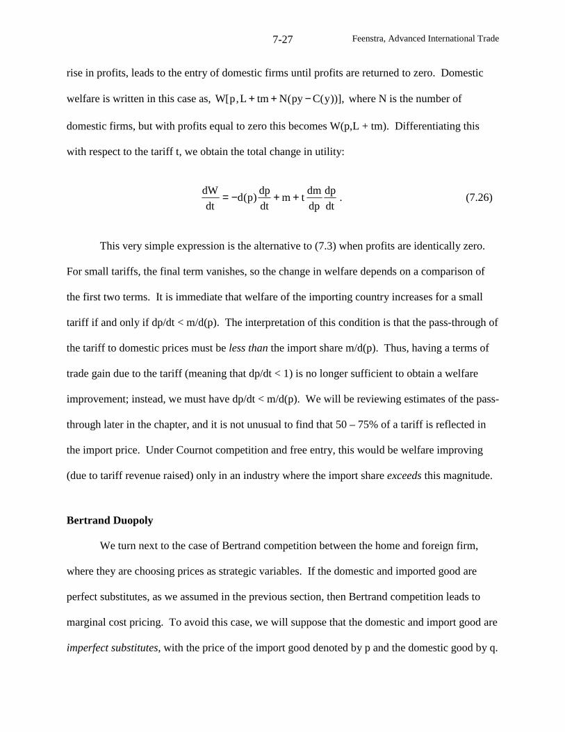
Feenstra, Advanced International Trade7-27
rise in profits, leads to the entry of domestic firms until profits are returned to zero. Domestic
welfare is written in this case as, ))],y(Cpy(NtmL,p[W −++ where N is the number of
domestic firms, but with profits equal to zero this becomes W(p,L + tm). Differentiating this
with respect to the tariff t, we obtain the total change in utility:
.dt
dp
dp
dmtm
dt
dp)p(d
dt
dW ++−= (7.26)
This very simple expression is the alternative to (7.3) when profits are identically zero.
For small tariffs, the final term vanishes, so the change in welfare depends on a comparison of
the first two terms. It is immediate that welfare of the importing country increases for a small
tariff if and only if dp/dt < m/d(p). The interpretation of this condition is that the pass-through of
the tariff to domestic prices must be less than the import share m/d(p). Thus, having a terms of
trade gain due to the tariff (meaning that dp/dt < 1) is no longer sufficient to obtain a welfare
improvement; instead, we must have dp/dt < m/d(p). We will be reviewing estimates of the pass-
through later in the chapter, and it is not unusual to find that 50 – 75% of a tariff is reflected in
the import price. Under Cournot competition and free entry, this would be welfare improving
(due to tariff revenue raised) only in an industry where the import share exceeds this magnitude.
Bertrand Duopoly
We turn next to the case of Bertrand competition between the home and foreign firm,
where they are choosing prices as strategic variables. If the domestic and imported good are
perfect substitutes, as we assumed in the previous section, then Bertrand competition leads to
marginal cost pricing. To avoid this case, we will suppose that the domestic and import good are
imperfect substitutes, with the price of the import good denoted by p and the domestic good by q.
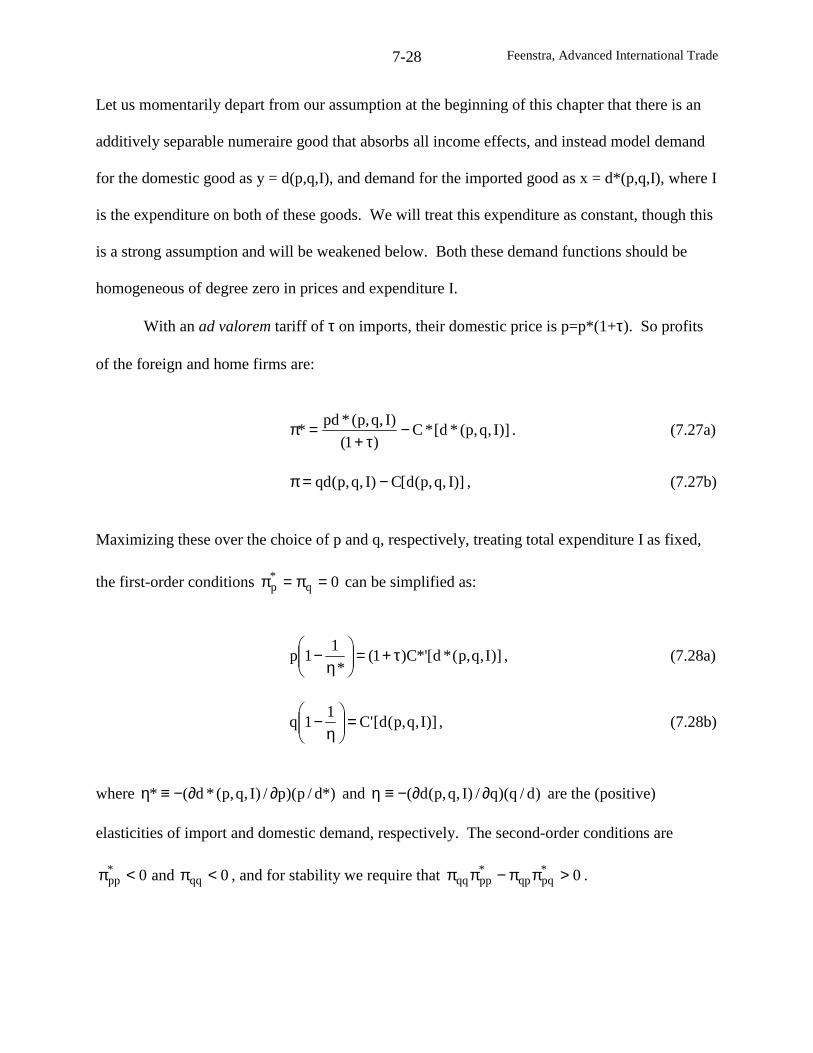
Feenstra, Advanced International Trade7-28
Let us momentarily depart from our assumption at the beginning of this chapter that there is an
additively separable numeraire good that absorbs all income effects, and instead model demand
for the domestic good as y = d(p,q,I), and demand for the imported good as x = d*(p,q,I), where I
is the expenditure on both of these goods. We will treat this expenditure as constant, though this
is a strong assumption and will be weakened below. Both these demand functions should be
homogeneous of degree zero in prices and expenditure I.
With an ad valorem tariff of τ on imports, their domestic price is p=p*(1+τ). So profits
of the foreign and home firms are:
)]I,q,p(*d[*C)1(
)I,q,p(*pd* −
τ+=π . (7.27a)
)]I,q,p(d[C)I,q,p(qd −=π , (7.27b)
Maximizing these over the choice of p and q, respectively, treating total expenditure I as fixed,
the first-order conditions 0q*p =π=π can be simplified as:
)]I,q,p(*d[*'C)1(*
11p τ+=
η
− , (7.28a)
)]I,q,p(d['C1
1q =
η
− , (7.28b)
where *)d/p)(p/)I,q,p(*d(* ∂∂−≡η and )d/q)(q/)I,q,p(d( ∂∂−≡η are the (positive)
elasticities of import and domestic demand, respectively. The second-order conditions are
0and0 qq*pp <π<π , and for stability we require that 0*
pqqp*ppqq >ππ−ππ .
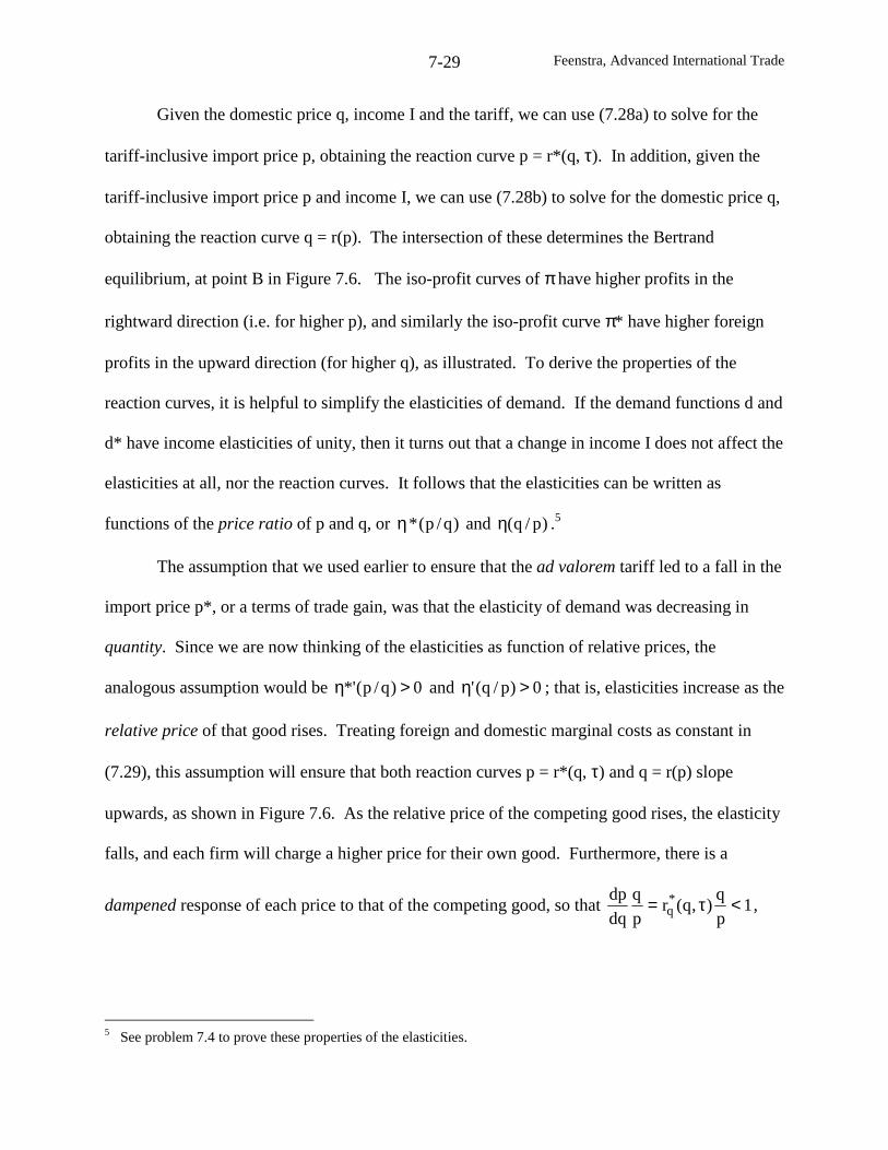
Feenstra, Advanced International Trade7-29
Given the domestic price q, income I and the tariff, we can use (7.28a) to solve for the
tariff-inclusive import price p, obtaining the reaction curve p = r*(q, τ). In addition, given the
tariff-inclusive import price p and income I, we can use (7.28b) to solve for the domestic price q,
obtaining the reaction curve q = r(p). The intersection of these determines the Bertrand
equilibrium, at point B in Figure 7.6. The iso-profit curves of πhave higher profits in the
rightward direction (i.e. for higher p), and similarly the iso-profit curve π* have higher foreign
profits in the upward direction (for higher q), as illustrated. To derive the properties of the
reaction curves, it is helpful to simplify the elasticities of demand. If the demand functions d and
d* have income elasticities of unity, then it turns out that a change in income I does not affect the
elasticities at all, nor the reaction curves. It follows that the elasticities can be written as
functions of the price ratio of p and q, or )q/p(*η and )p/q(η .5
The assumption that we used earlier to ensure that the ad valorem tariff led to a fall in the
import price p*, or a terms of trade gain, was that the elasticity of demand was decreasing in
quantity. Since we are now thinking of the elasticities as function of relative prices, the
analogous assumption would be 0)q/p(*' >η and 0)p/q(' >η ; that is, elasticities increase as the
relative price of that good rises. Treating foreign and domestic marginal costs as constant in
(7.29), this assumption will ensure that both reaction curves p = r*(q, τ) and q = r(p) slope
upwards, as shown in Figure 7.6. As the relative price of the competing good rises, the elasticity
falls, and each firm will charge a higher price for their own good. Furthermore, there is a
dampened response of each price to that of the competing good, so that 1p
q),q(r
p
q
dq
dp *q <τ= ,
5 See problem 7.4 to prove these properties of the elasticities.
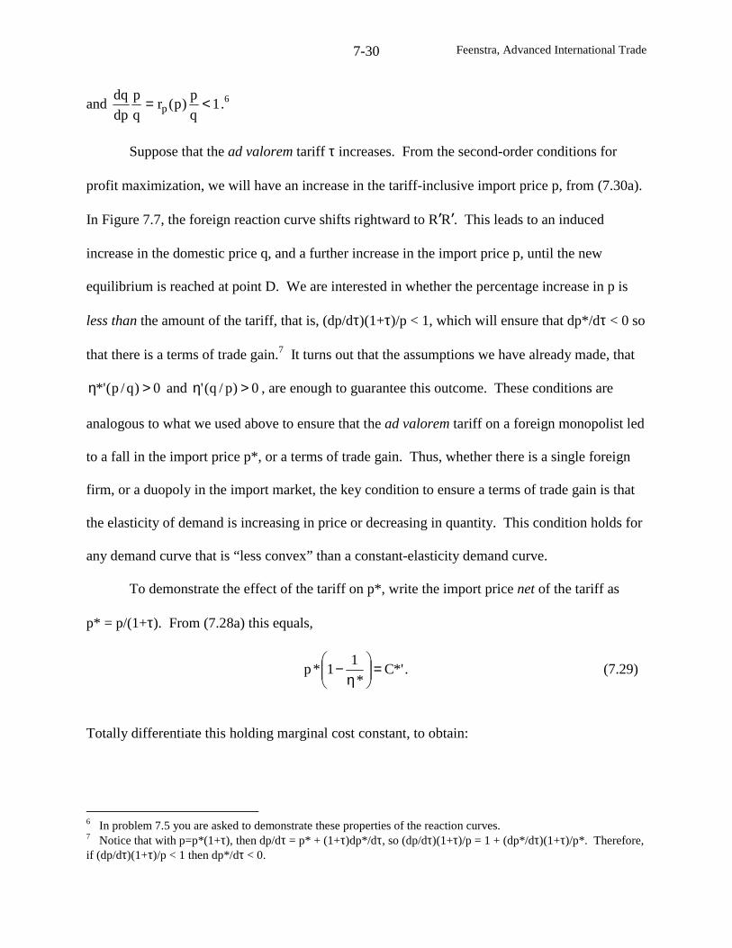
Feenstra, Advanced International Trade7-30
and 1q
p)p(r
q
p
dp
dqp <= .6
Suppose that the ad valorem tariff τ increases. From the second-order conditions for
profit maximization, we will have an increase in the tariff-inclusive import price p, from (7.30a).
In Figure 7.7, the foreign reaction curve shifts rightward to R’R’. This leads to an induced
increase in the domestic price q, and a further increase in the import price p, until the new
equilibrium is reached at point D. We are interested in whether the percentage increase in p is
less than the amount of the tariff, that is, (dp/dτ)(1+τ)/p < 1, which will ensure that dp*/dτ < 0 so
that there is a terms of trade gain.7 It turns out that the assumptions we have already made, that
0)q/p(*' >η and 0)p/q(' >η , are enough to guarantee this outcome. These conditions are
analogous to what we used above to ensure that the ad valorem tariff on a foreign monopolist led
to a fall in the import price p*, or a terms of trade gain. Thus, whether there is a single foreign
firm, or a duopoly in the import market, the key condition to ensure a terms of trade gain is that
the elasticity of demand is increasing in price or decreasing in quantity. This condition holds for
any demand curve that is “less convex” than a constant-elasticity demand curve.
To demonstrate the effect of the tariff on p*, write the import price net of the tariff as
p* = p/(1+τ). From (7.28a) this equals,
*'C*
11*p =
η
− . (7.29)
Totally differentiate this holding marginal cost constant, to obtain:
6 In problem 7.5 you are asked to demonstrate these properties of the reaction curves.7 Notice that with p=p*(1+τ), then dp/dτ = p* + (1+τ)dp*/dτ, so (dp/dτ)(1+τ)/p = 1 + (dp*/dτ)(1+τ)/p*. Therefore,if (dp/dτ)(1+τ)/p < 1 then dp*/dτ < 0.
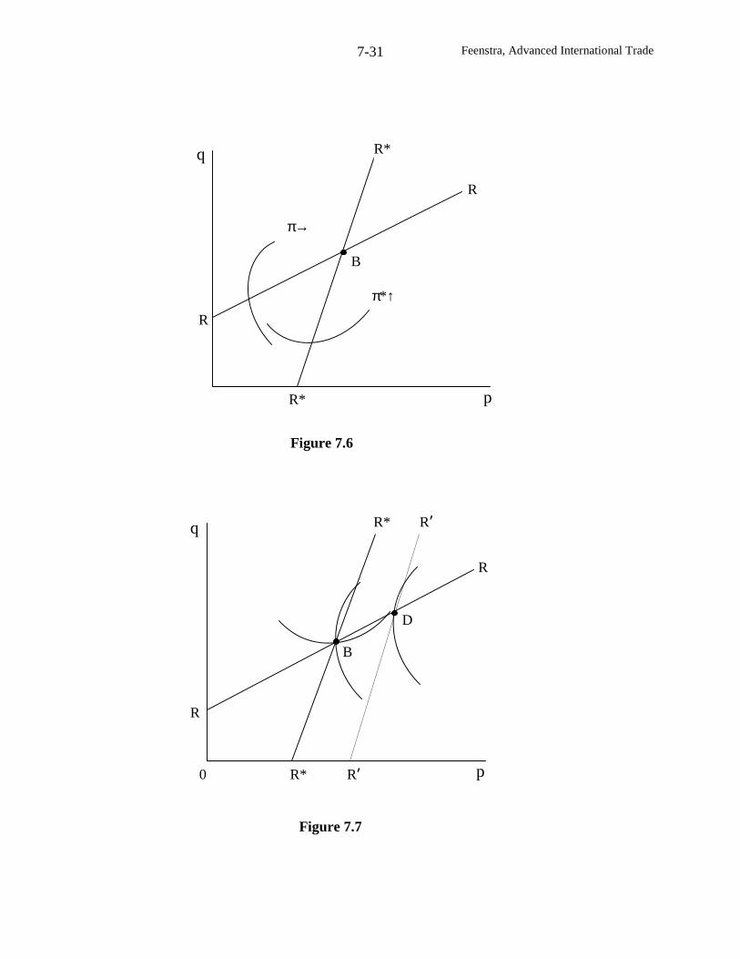
Feenstra, Advanced International Trade7-31
R
q
pR*
π→
B
R
R*
π*↑
Figure 7.7
D
B
R
q
0 R* R’ p
R* R’
R
Figure 7.6
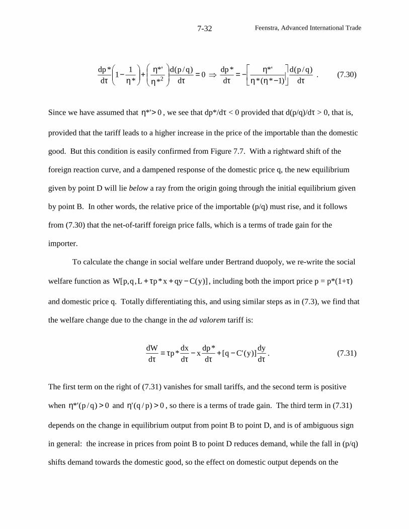
Feenstra, Advanced International Trade7-32
τ
−ηη
η−=τ
⇒=τ
ηη+
η
−τ d
)q/p(d
)1*(*
*'
d
*dp0
d
)q/p(d
*
*'
*
11
d
*dp2
. (7.30)
Since we have assumed that 0*'>η , we see that dp*/dτ < 0 provided that d(p/q)/dτ > 0, that is,
provided that the tariff leads to a higher increase in the price of the importable than the domestic
good. But this condition is easily confirmed from Figure 7.7. With a rightward shift of the
foreign reaction curve, and a dampened response of the domestic price q, the new equilibrium
given by point D will lie below a ray from the origin going through the initial equilibrium given
by point B. In other words, the relative price of the importable (p/q) must rise, and it follows
from (7.30) that the net-of-tariff foreign price falls, which is a terms of trade gain for the
importer.
To calculate the change in social welfare under Bertrand duopoly, we re-write the social
welfare function as )]y(Cqyx*pL,q,p[W −+τ+ , including both the import price p = p*(1+τ)
and domestic price q. Totally differentiating this, and using similar steps as in (7.3), we find that
the welfare change due to the change in the ad valorem tariff is:
τ−+
τ−
ττ=
τ d
dy)]y('Cq[
d
*dpx
d
dx*p
d
dW. (7.31)
The first term on the right of (7.31) vanishes for small tariffs, and the second term is positive
when 0)q/p(*' >η and 0)p/q(' >η , so there is a terms of trade gain. The third term in (7.31)
depends on the change in equilibrium output from point B to point D, and is of ambiguous sign
in general: the increase in prices from point B to point D reduces demand, while the fall in (p/q)
shifts demand towards the domestic good, so the effect on domestic output depends on the
Feenstra, Advanced International Trade7-33
relative strength of these effects. It turns out that if the increase in domestic price is not too
large, then an increase is domestic output occurs. The condition to ensure this is that the
elasticity of the home reaction curve does not exceed
η−η<= 1
q
p)p(r
q
p
dp
dqp .8 In that case,
domestic output increases due to the tariff, which generates a welfare gain additional to the terms
of trade gain.
The finding that domestic output may rise due to the tariff depends on our maintained
assumption that total expenditure I on the import and domestic products is constant. This would
apply, for example, with a Cobb-Douglas utility function between an aggregate of the products
(d, d*) and all other goods in the economy, but would not be true otherwise. Generally, total
expenditure on the import and domestic products can rise or fall due to the tariff, and the latter
case could lead to a fall in domestic output and a welfare loss.9 So the “profit shifting” motive
for import protection is not that robust, as we also found under Cournot competition. Instead, the
terms of trade motive for tariffs becomes the best indicator of gain or loss for the importing
country. Under our assumptions that the elasticity of demand is increasing in price or decreasing
in quantity, there is a terms of trade gain for the importer, and the optimal tariff is positive for
that reason. Conversely, with constant elasticities of demand the optimal tariff is zero. Finally,
in the somewhat unusual case where the elasticity of demand is decreasing in price or increasing
in quantity, then an import subsidy is optimal.
8 See problem 7.6.9 The change in domestic output due to tariffs is investigated in a monopolistic competition model by Helpman(1990), using a utility function that allows for expenditure on the differentiated good to change. He confirms thatoutput of the domestic good can rise or fall due to the tariff. The latter possibility was first suggested by Markusen(1990), who referred to the phenomena as a “de-rationalizing tariff.” This might hold, for example, if the importedgoods are intermediate inputs, and the tariff leads to reduced sales of the industry using the inputs. This was foundto hold in a simulation model of the Mexican automobile industry by Lopez de Silanes, et al (1994).
Feenstra, Advanced International Trade7-34
Tariffs on Japanese Truck and Motorcycles
We have found that with imperfect competition, a terms of trade argument for a tariff is
likely but not guaranteed. The “strategic” response of foreign firms in adjusting their price p*
then becomes an interesting empirical question. Feenstra (1989) provides some empirical
evidence on this for two U.S. tariffs initially applied during the early 1980s: a 25% tariff on
imports of compact trucks, coming from Japan; and a temporary, declining tariff beginning at
45% on imports of heavyweight motorcycles from Japan. The history of how these tariffs came
to be applied is itself an important lesson in trade policy.
In 1979, Paul Volcker was appointed as Chairman of the Board of Governors of the
Federal Reserve Bank in the United States. Inflation exceeded 10%, and showed signs of getting
worse, so Volcker was committed to bring this down. A period of tight monetary policy
followed, which led to very high interest rates, a strong dollar and a deep recession beginning in
January 1980. There may well have been long-term gains resulting from this policy, since
following the recovery from the recession in late 1982, the U.S. began nearly two decades of
expansion, interrupted only by a mild recession in 1990-91. But at the same time, there were
short-term costs in terms of unemployment, and one of the sectors hardest hit was automobiles.
Accordingly, in June 1980 the United Automobile Workers applied to the ITC for
protection, under Section 201 of U.S. trade laws. A similar petition was received in August 1980
from Ford Motor Company. As described at the beginning of the chapter, Section 201 protection
can be given when increased imports are a “substantial cause of serious injury to the domestic
industry,” where “substantial cause” must be “not less than any other cause.” In fact, the ITC
determined that the U.S. recession was a more important cause of injury in autos than were
increased imports. Accordingly, it did not recommend that the auto industry receive protection.
Feenstra, Advanced International Trade7-35
With this negative determination, several congressmen from mid-western states
continued to pursue import limits by other means. For cars imported for Japan, this protection
took the form of a “voluntary” restraint on the quantity of imports, as described in the next
chapter. For trucks imported from Japan, however, another form of protection was available.
During the 1970s, Japan had exported an increasing number of compact trucks to the U.S., most
as cab/chassis with some final assembly needed. These were classified as “parts of trucks,”
which carried a tariff rate of 4%, whereas “complete or unfinished trucks” carried a tariff rate of
25%. That unusually high tariff was a result of the “Chicken War” between the U.S. and West
Germany in 1962. At that time, Germany joined the European Economic Community (EEC),
and was required to adjust its external tariffs to match those of the other EEC countries. This
resulted in an increase in its tariff on poultry, which was imported from the United States. In
retaliation, the U.S. increased its tariffs on “complete or unfinished trucks” and other products,
so the 25% tariff on trucks became a permanent item of the U.S. tariff code. With prodding from
the Congress, in 1980 the U.S. Customs Service announced that effective August 21 import
lightweight cab/chassis would be reclassified as complete trucks. This raised the tariff rates on
nearly all Japanese trucks from 4% to 25%, which remains in effect today.10
A second increase in tariffs occurred during the 1980s on heavyweight motorcycles (i.e.
over 700 cc displacement), produced by Harley-Davidson. That company also applied to the
ITC for Section 201 protection, in 1983. It was being impacted not so much by the U.S.
recession, as from a long period of lagging productivity combined with intense competition from
Japanese producers. Two of these (Honda and Kawasaki) had plants in the U.S. and also
imported, whereas two others (Suzuki and Yamaha) produced and exported from Japan. In the
10 Japanese producers sued in U.S. court to have the reclassification reversed, but lost that case.
Feenstra, Advanced International Trade7-36
early 1980s, these firms were engaged in global price war that spilled over into the U.S. market.
As a result, inventories of imported heavyweight cycles rose dramatically in the United States:
the ITC estimated that inventories as of September 1982 exceeded actual U.S. consumption
during January – September of that year (USITC, 1983, p. 13).
From our description of Section 201 at the beginning of the chapter, recall that protection
can be recommended if increased imports are a “substantial cause of serious injury, or threat
thereof, to the domestic industry.” The very high level of inventories held by Japanese
producers was judged by the ITC to be a threat to the domestic industry, and protection was
indeed granted. This protection took the form of a five-year declining tariff schedule: 45%
effective April 16, 1983, and then declining annually to 35%, 20%, 15% and 10%, and scheduled
to end in April 1988.11 In fact, Harley-Davidson petitioned the ITC to end the tariff early, after
the 15% rate expired in 1987, by which time it had cut costs and introduced new and very
popular products, so profitability had been restored.
U.S. imports of compact trucks and heavyweight cycles from Japan provide ideal
industry cases to study the pass-though of the tariffs to U.S. prices. We are especially interested
in whether Japanese producers absorbed part of the tariff, which would be a terms of trade gain
for the United States, or whether they fully passed it through to U.S. prices. There are few
studies of the pass-through of tariffs, but many studies of the pass-through of exchange rates, i.e.
the response of import prices to change in the value of the exporter’s currency. Most studies at
either the aggregate or disaggregate level suggest that the pass-through of exchange rates is less
11 Actually, the protection took the form of a “tariff-rate quota,” which means that the declining tariffs rates wereapplied to imports of heavyweight motorcycles from each source country when imports exceeded a quota limit forthe exporting country. The U.S. was also importing heavyweight cycles from BMW in Germany, but that countrywas granted a quota large enough that none of the imports were subject to the tariff. In contrast, Japan was allocateda quota (ranging from 6,000 to 10,000 units per year) that was less than its imports, so that declining tariffs appliedto all imports in excess of this amount.
Feenstra, Advanced International Trade7-37
than complete, and averages about 0.6 (Goldberg and Knetter, 1997, p. 1250), though this
depends on the industry being studied.12 We will argue below that the pass-through of tariffs and
exchange rates ought to be “symmetric” in a given industry, and will test this hypothesis for
trucks and motorcycles. In addition, we will include U.S. import of Japanese cars before the
VER in our sample, though for that product we will only estimate the pass-through of the
exchange rate.
Estimating the Terms of Trade Effect
To obtained an estimating equation, let us begin with the first-order condition of a typical
foreign exporter, in (7.28a), where we treat foreign marginal costs C*’ as constant, and re-write
this as c*, in the foreign currency. We need to convert this to the domestic currency using an
expected exchange rate e, so we re-write (7.28a) as:
*ec)1(*
11p τ+=
η
− . (7.32)
Using the assumption that the income elasticity of demand is unity, we express the elasticity of
import demand, η*(p/q), as a function of the import/domestic price ratio. More generally,
η*(p,q,I) will depend on consumer income, too, but is homogeneous of degree zero in (p,q,I).13
So treating the domestic price, income, tariff rate, exchange rate and foreign marginal cost as
parameters, (7.32) is one equation in one unknown – the import price p. We can therefore solve
for the import prices as a function of the parameters,
12 The disaggregate results of Knetter (1989, 1993) show that exchange rate pass-through varies quite substantiallyacross products and source countries, with U.S. exporters absorbing the least of any exchange rate change. In recentwork, Campa and Goldberg (2002) investigate the pass-through of exchange rates in broad import sectors of theOECD countries, and find average long run elasticities ranging from 0.61 – 0.89 across sectors.13 See problem 7.4.
Feenstra, Advanced International Trade7-38
].I,q*,ec)1[(p τ+φ= (7.33)
With η*(p,q,I) homogeneous of degree zero in (p,q,I), it is readily verified that
]I,q*,ec)1[( τ+φ is homogeneous of degree one in its arguments. This is our first testable
hypothesis, which checks the overall specification of the pricing equation. Second, notice that
we have written the tariff, exchange rate and marginal costs as multiplied together in the
arguments of ]I,q*,ec)1[( τ+φ , because that is how they appear in the first-order condition
(7.32). This is another testable hypothesis. To implement both these tests, let us specify (7.33)
as a log-linear function of its arguments, which are indexed by time t:
( ) ttjt
L
0i
M
1jjtit
*titt Ilnqln)1ln(sclnpln ε+δ+γ+τ+β+β+α= ∑ ∑
= =− . (7.34)
The first term on the right of (7.34), αt, is a simple quadratic function of time, which will
allow import price to change in a smooth fashion for reasons not specified elsewhere in the
equation. To obtain the second term, we specify that the expected exchange rate et is a weighted
average of lagged spot rates, its − , i = 0,1,…,L (in $/yen). This allows us to write )scln( it*t − as
having the coefficients iβ , i = 0,1,…,L, the sum of which will indicate the total pass-through of
the exchange rate to import prices. Next, we write the ad valorem tariff )1ln( tτ+ as having the
coefficient β, which is the pass-through of the tariff. The hypothesis of symmetric pass-through
of the tariff and exchange rate is therefore tested as:
β=β∑=
L
0ii . (7.35a)
Feenstra, Advanced International Trade7-39
The next terms appearing on the right of (7.34) are the price of domestic or rival import
products, j=1,…,M. For Japanese imports, this would include the average price of U.S. products,
as well as German imported cars or motorcycles. Finally, total consumer expenditure on the
broad category of transportation equipment is included as a measure of “income.” Notice that if
the income elasticity of demand is unity, then the foreign elasticity η*(p/q) does not depend on I,
and neither will the optimal price pt in (7.34), so δ=0. In any case, the hypothesis that the whole
equation is homogeneous of degree one can be tested by:
1j
M
1ji
L
0i=δ+γ+β ∑∑
==(7.35b)
The results of estimating (7.34) using quarterly data for U.S. imports are shown in Table
7.2. The first row indicates the sample period of quarterly data used for each product. There are
two distinct samples used for heavyweight motorcycles. The first sample consists of interview
data reported by the United States ITC (1983, Table 8 and 1983-84). The advantage of this data
is that it gives the unit-value of imports for consumption, inclusive of duty, for the major
Japanese importers (Honda, Suzuki and Yamaha). However, the disadvantage is that the data
end in 1984:4 and include a small amount of German heavyweight motorcycles within the
reported unit-value. A second source was collected at the border by the U.S. Dept of Commerce
giving the unit-value of imports shipments, distinguishing Japanese and German heavyweight
cycles up to 1987:1.14 We experiment with both data sources, and also the pooled sample.
In the first regression of Table 7.2 for Japanese imported cars, the coefficients on the
exchange rate terms sum to 0.71, which is the estimate of the pass-through elasticity. For
Japanese imported trucks, the sum of coefficients on the exchange rates is 0.63, while the
14 Import shipments include motorcycles going into inventory. These data were adjusted to include the tariff.
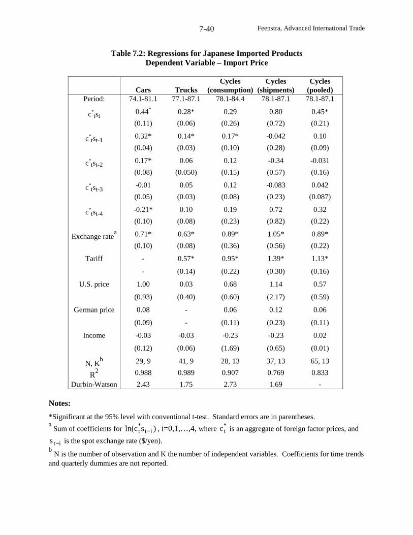
Feenstra, Advanced International Trade7-40
Table 7.2: Regressions for Japanese Imported ProductsDependent Variable – Import Price
Cycles Cycles CyclesCars Trucks (consumption) (shipments) (pooled)
Period: 74.1-81.1 77.1-87.1 78.1-84.4 78.1-87.1 78.1-87.1
c*tst
0.44* 0.28* 0.29 0.80 0.45*
(0.11) (0.06) (0.26) (0.72) (0.21)
c*tst-1
0.32* 0.14* 0.17* -0.042 0.10
(0.04) (0.03) (0.10) (0.28) (0.09)
c*tst-2
0.17* 0.06 0.12 -0.34 -0.031
(0.08) (0.050) (0.15) (0.57) (0.16)
c*tst-3
-0.01 0.05 0.12 -0.083 0.042
(0.05) (0.03) (0.08) (0.23) (0.087)
c*tst-4
-0.21* 0.10 0.19 0.72 0.32
(0.10) (0.08) (0.23) (0.82) (0.22)
Exchange ratea 0.71* 0.63* 0.89* 1.05* 0.89*
(0.10) (0.08) (0.36) (0.56) (0.22)
Tariff - 0.57* 0.95* 1.39* 1.13*
- (0.14) (0.22) (0.30) (0.16)
U.S. price 1.00 0.03 0.68 1.14 0.57
(0.93) (0.40) (0.60) (2.17) (0.59)
German price 0.08 - 0.06 0.12 0.06
(0.09) - (0.11) (0.23) (0.11)
Income -0.03 -0.03 -0.23 -0.23 0.02
(0.12) (0.06) (1.69) (0.65) (0.01)
N, Kb 29, 9 41, 9 28, 13 37, 13 65, 13
R2 0.988 0.989 0.907 0.769 0.833
Durbin-Watson 2.43 1.75 2.73 1.69 -
Notes:
*Significant at the 95% level with conventional t-test. Standard errors are in parentheses.a
Sum of coefficients for )scln( it*t − , i=0,1,…,4, where *
tc is an aggregate of foreign factor prices, and
its − is the spot exchange rate ($/yen).b
N is the number of observation and K the number of independent variables. Coefficients for time trendsand quarterly dummies are not reported.
Feenstra, Advanced International Trade7-41
coefficient on the tariff is 0.57. The hypothesis (7.35a) that these are equal is easily accepted, as
is hypothesis (7.35b) that the pricing equation is homogeneous of degree one. When both of
these restrictions are imposed then the pass-through elasticity (for the exchange rate or the tariff)
becomes 0.58. Thus, there is strong evidence that the increase in the truck tariff was only
partially reflected in U.S. prices: of the 21% increase, about 0.58⋅21 = 12% was passed through
to U.S. prices, whereas the other 9% was absorbed by Japanese producers, leading to a terms of
trade gain for the United States.
For Japanese imports of heavyweight motorcycles, however, the story is quite different.
Regardless of which sample is used (consumption, shipments, or pooled), we find that the pass-
through of the exchange rate or the tariff are both insignificantly different from unity! So while
the hypothesis (7.35a) of “symmetric” pass-through is still confirmed, as is (7.35b), it is no
longer the case that the United States experienced a terms of trade gain in this product. Rather,
the full amount of the tariff in each year was passed through to U.S. prices.
What explains the differing results for compact trucks and heavyweight motorcycles? In
the case of trucks, we note that prior to the increase of the tariff in August 1980, nearly all
compact trucks sold in the U.S. were produced by Japanese firms, some of which were marketed
through American auto companies. But after the tariff was imposed, U.S. producers introduced
their own compact truck models, with very similar characteristics to the Japanese imports (see
Feenstra, 1988). The Japanese producers (Isuzu and Mitsubishi) that had formerly been selling
to American firms began to market compact trucks independently. In this environment of
relatively intense competition, we can expect that Japanese firms would be reluctant to pass-
through the full amount of the tariff and risk losing more market share in the United States.
Feenstra, Advanced International Trade7-42
In heavyweight motorcycles, by contrast, recall that there was already a global price war,
so that prices were likely close to marginal cost. This leaves little room for Japanese producers
to absorb part of the tariff. This is reinforced by the fact that the tariff was temporary, and that
U.S. inventories were high: there would be little reason to sell to the U.S. at a reduced price in
one year, if instead sales could be made out of inventory and some exports delayed to a later year
when the tariff was lower.15 By this logic, it is not surprising that the pass-through of the tariff in
motorcycles was complete.
How should we assess the efficacy of the tariff in these two products? The tariff on
trucks led to a terms of trade gain, and if this exceeds the deadweight loss, then it would generate
a welfare gain for the United States. This is not the case for the tariff on motorcycles, however,
where there is a deadweight loss but no offsetting terms of trade gain. By our conventional
welfare criterion, then, the tariff on trucks looks better than the tariff on heavyweight cycles. But
this criterion ignores the fact that the tariff on motorcycles was temporary, whereas that on
trucks is still in place today. Furthermore, it is well documented (see Reid, 1990) that Harley-
Davidson was on the brink of bankruptcy in 1982-83, and was able to secure a bank loan only
after receiving protection, so the tariff may well have contributed to its continued survival. Its
near-bankrupt status was due to problems of poor management and lagging productivity, while
its revival after 1983 was due to the introduction of improved products and production
techniques. It cannot be argued that this broad change in company practices was caused by the
tariff, but it appears that the temporary tariff bought it some breathing room.16 In view of the
15 It was still the case that exports from Japan of heavyweight motorcycles (over 700 cc) were positive in everyyear of the tariff. In addition, Japanese firms began to sell a 699 cc motorcycle in the United States, which was away to evade the tariff. See the discussion in Irwin (2002, pp. 135-137).16 This is the view expressed by the chief economist at the ITC at the time: “if the case of heavyweight motorcyclesis to be considered the only successful escape-clause, it is because it caused little harm and it helped Harley-Davidson get a bank loan so it could diversify” [Suomela (1993, p. 135) as cited by Irwin (2002, pp. 136-37)].
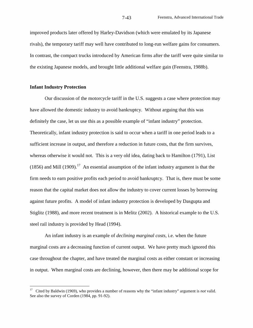
Feenstra, Advanced International Trade7-43
improved products later offered by Harley-Davidson (which were emulated by its Japanese
rivals), the temporary tariff may well have contributed to long-run welfare gains for consumers.
In contrast, the compact trucks introduced by American firms after the tariff were quite similar to
the existing Japanese models, and brought little additional welfare gain (Feenstra, 1988b).
Infant Industry Protection
Our discussion of the motorcycle tariff in the U.S. suggests a case where protection may
have allowed the domestic industry to avoid bankruptcy. Without arguing that this was
definitely the case, let us use this as a possible example of “infant industry” protection.
Theoretically, infant industry protection is said to occur when a tariff in one period leads to a
sufficient increase in output, and therefore a reduction in future costs, that the firm survives,
whereas otherwise it would not. This is a very old idea, dating back to Hamilton (1791), List
(1856) and Mill (1909).17 An essential assumption of the infant industry argument is that the
firm needs to earn positive profits each period to avoid bankruptcy. That is, there must be some
reason that the capital market does not allow the industry to cover current losses by borrowing
against future profits. A model of infant industry protection is developed by Dasgupta and
Stiglitz (1988), and more recent treatment is in Melitz (2002). A historical example to the U.S.
steel rail industry is provided by Head (1994).
An infant industry is an example of declining marginal costs, i.e. when the future
marginal costs are a decreasing function of current output. We have pretty much ignored this
case throughout the chapter, and have treated the marginal costs as either constant or increasing
in output. When marginal costs are declining, however, then there may be additional scope for
17 Cited by Baldwin (1969), who provides a number of reasons why the “infant industry” argument is not valid.See also the survey of Corden (1984, pp. 91-92).
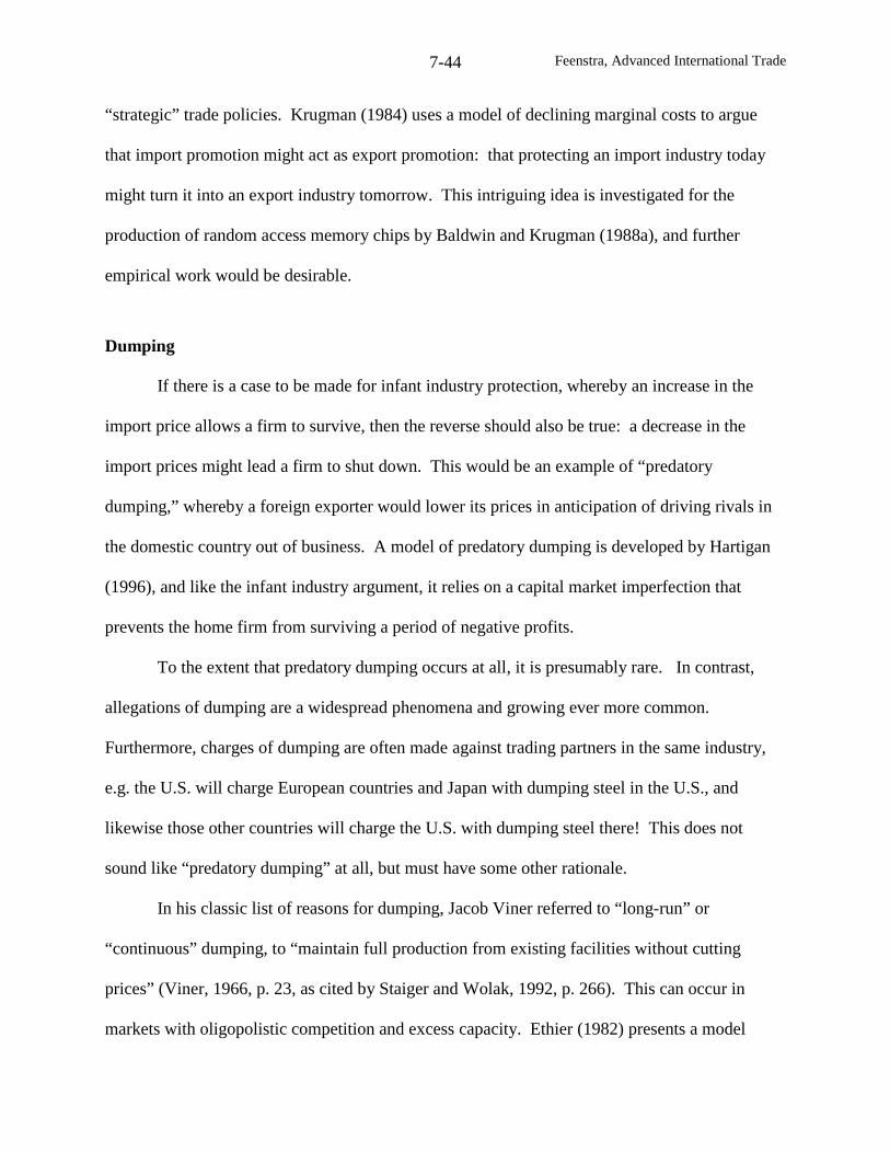
Feenstra, Advanced International Trade7-44
“strategic” trade policies. Krugman (1984) uses a model of declining marginal costs to argue
that import promotion might act as export promotion: that protecting an import industry today
might turn it into an export industry tomorrow. This intriguing idea is investigated for the
production of random access memory chips by Baldwin and Krugman (1988a), and further
empirical work would be desirable.
Dumping
If there is a case to be made for infant industry protection, whereby an increase in the
import price allows a firm to survive, then the reverse should also be true: a decrease in the
import prices might lead a firm to shut down. This would be an example of “predatory
dumping,” whereby a foreign exporter would lower its prices in anticipation of driving rivals in
the domestic country out of business. A model of predatory dumping is developed by Hartigan
(1996), and like the infant industry argument, it relies on a capital market imperfection that
prevents the home firm from surviving a period of negative profits.
To the extent that predatory dumping occurs at all, it is presumably rare. In contrast,
allegations of dumping are a widespread phenomena and growing ever more common.
Furthermore, charges of dumping are often made against trading partners in the same industry,
e.g. the U.S. will charge European countries and Japan with dumping steel in the U.S., and
likewise those other countries will charge the U.S. with dumping steel there! This does not
sound like “predatory dumping” at all, but must have some other rationale.
In his classic list of reasons for dumping, Jacob Viner referred to “long-run” or
“continuous” dumping, to “maintain full production from existing facilities without cutting
prices” (Viner, 1966, p. 23, as cited by Staiger and Wolak, 1992, p. 266). This can occur in
markets with oligopolistic competition and excess capacity. Ethier (1982) presents a model
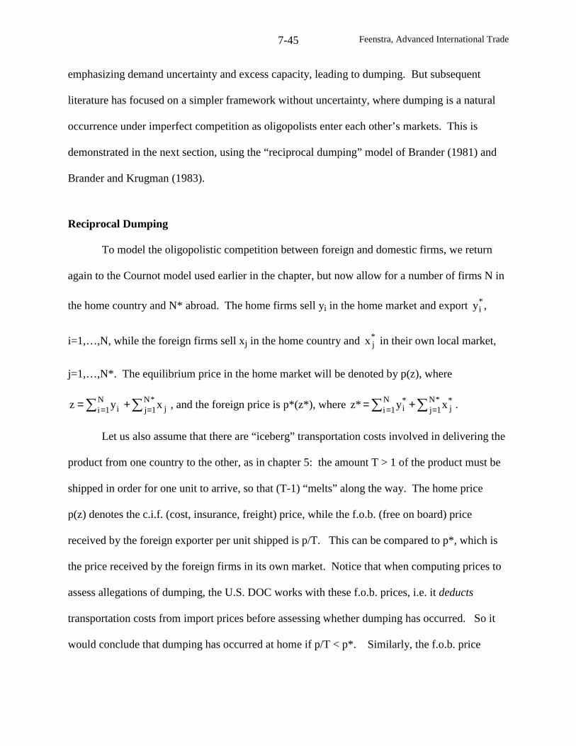
Feenstra, Advanced International Trade7-45
emphasizing demand uncertainty and excess capacity, leading to dumping. But subsequent
literature has focused on a simpler framework without uncertainty, where dumping is a natural
occurrence under imperfect competition as oligopolists enter each other’s markets. This is
demonstrated in the next section, using the “reciprocal dumping” model of Brander (1981) and
Brander and Krugman (1983).
Reciprocal Dumping
To model the oligopolistic competition between foreign and domestic firms, we return
again to the Cournot model used earlier in the chapter, but now allow for a number of firms N in
the home country and N* abroad. The home firms sell yi in the home market and export *iy ,
i=1,…,N, while the foreign firms sell xj in the home country and *jx in their own local market,
j=1,…,N*. The equilibrium price in the home market will be denoted by p(z), where
∑∑ == += *N1j j
N1i i xyz , and the foreign price is p*(z*), where ∑∑ == += *N
1j*j
N1i
*i xy*z .
Let us also assume that there are “iceberg” transportation costs involved in delivering the
product from one country to the other, as in chapter 5: the amount T > 1 of the product must be
shipped in order for one unit to arrive, so that (T-1) “melts” along the way. The home price
p(z) denotes the c.i.f. (cost, insurance, freight) price, while the f.o.b. (free on board) price
received by the foreign exporter per unit shipped is p/T. This can be compared to p*, which is
the price received by the foreign firms in its own market. Notice that when computing prices to
assess allegations of dumping, the U.S. DOC works with these f.o.b. prices, i.e. it deducts
transportation costs from import prices before assessing whether dumping has occurred. So it
would conclude that dumping has occurred at home if p/T < p*. Similarly, the f.o.b. price
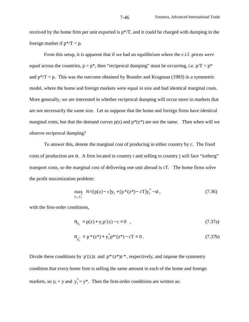
Feenstra, Advanced International Trade7-46
received by the home firm per unit exported is p*/T, and it could be charged with dumping in the
foreign market if p*/T < p.
From this setup, it is apparent that if we had an equilibrium where the c.i.f. prices were
equal across the countries, p = p*, then “reciprocal dumping” must be occurring, i.e. p/T < p*
and p*/T < p. This was the outcome obtained by Brander and Krugman (1983) in a symmetric
model, where the home and foreign markets were equal in size and had identical marginal costs.
More generally, we are interested in whether reciprocal dumping will occur more in markets that
are not necessarily the same size. Let us suppose that the home and foreign firms have identical
marginal costs, but that the demand curves p(z) and p*(z*) are not the same. Then when will we
observe reciprocal dumping?
To answer this, denote the marginal cost of producing in either country by c. The fixed
costs of production are α. A firm located in country i and selling to country j will face “iceberg”
transport costs, so the marginal cost of delivering one unit abroad is cT. The home firms solve
the profit maximization problem:
α−−+−=π *ii
y,yy]cT*)z(*p[y]c)z(p[max
*ii
, (7.36)
with the first-order conditions,
0c)z('py)z(p iyi=−+=π , (7.37a)
0cT*)z(*'py*)z(*p *iy*
i=−+=π . (7.37b)
Divide these conditions by z)z('p and *z*)z(*'p , respectively, and impose the symmetry
condition that every home firm is selling the same amount in each of the home and foreign
markets, so yi = y and *iy = y*. Then the first-order conditions are written as:

Feenstra, Advanced International Trade7-47
c)z/y(
1p =
η− , cT*
*)z/*y(1*p =
η− , (7.38)
where p)z('p/z=η and *p*)z(*'p/*z* =η are the home and foreign demand elasticities.
In a similar manner, we can derive the first-order conditions for the foreign firms,
c*
*)z/*x(1*p =
η− , cT)z/x(
1p =
η− (7.39)
where each of these firms is selling x* in its own market and x in the home market.
By adding up the market shares of all firms selling in each country, we must obtain:
N(y/z) + N*(x/z) = 1 ,(7.40)
N(y*/z*) + N*(x*/z*) = 1 .
Notice that we can write this simple system in matrix notation as:
)1,1(*)z/*x()z/x(
*)z/*y()z/y(*)N,N( =
, (7.40’)
which can be inverted to solve for the number of firms in each country:
−
−=
)z/y()z/x(
*)z/*y(*)z/*x(
D
)1,1(*)N,N( ⇒
,*z
*y
z
y
D
1*N
,z
x
*z
*x
D
1N
−=
−=
(7.41)
where D is the determinant of the 2x2 matrix of market shares shown in (7.40’). From the first-
order conditions (7.38) and (7.39) it is clear that (y/z) > (x/z) and (x*/z*) > (y*/z*), so that local
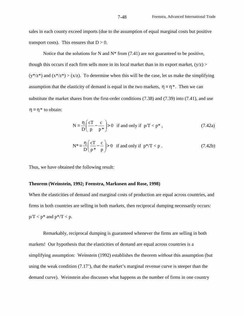
Feenstra, Advanced International Trade7-48
sales in each county exceed imports (due to the assumption of equal marginal costs but positive
transport costs). This ensures that D > 0.
Notice that the solutions for N and N* from (7.41) are not guaranteed to be positive,
though this occurs if each firm sells more in its local market than in its export market, (y/z) >
(y*/z*) and (x*/z*) > (x/z). To determine when this will be the case, let us make the simplifying
assumption that the elasticity of demand is equal in the two markets, *η=η . Then we can
substitute the market shares from the first-order conditions (7.38) and (7.39) into (7.41), and use
*η=η to obtain:
0*p
c
p
cT
DN >
−η= if and only if p/T < p* , (7.42a)
0p
c
*p
cT
D*N >
−η= if and only if p*/T < p . (7.42b)
Thus, we have obtained the following result:
Theorem (Weinstein, 1992; Feenstra, Markusen and Rose, 1998)
When the elasticities of demand and marginal costs of production are equal across countries, and
firms in both countries are selling in both markets, then reciprocal dumping necessarily occurs:
p/T < p* and p*/T < p.
Remarkably, reciprocal dumping is guaranteed whenever the firms are selling in both
markets! Our hypothesis that the elasticities of demand are equal across countries is a
simplifying assumption: Weinstein (1992) establishes the theorem without this assumption (but
using the weak condition (7.17’), that the market’s marginal revenue curve is steeper than the
demand curve). Weinstein also discusses what happens as the number of firms in one country
Feenstra, Advanced International Trade7-49
grows. As N* grows, the equilibrium price p* in the foreign market falls. For a sufficiently high
number of foreign firms, the inequality p/T < p* becomes an equality, and at this point the
number of domestic firms from (7.42a) is zero: import competition has eliminated the domestic
industry. However, note from (7.42b) that we still have p*/T < p, so that the foreign firms are
dumping into the domestic market. Thus, even when the number of firm in one country has
grown large enough to eliminate competition in the other, unilateral dumping still occurs.
Welfare Effect of Trade
This model of reciprocal dumping is an alternative explanation for “intra-industry” trade,
which we studied in chapter 5 under a monopolistic competition model. In that case, we argued
that trade would bring extra gains, due to the increased variety of products and also economies of
scale. But in the Cournot model we are studying, the firms are selling a homogeneous product so
that there are no gains due to product variety, but instead losses due to wasted transportation
costs in “cross hauling.” On the other hand, trade brings a reduction in the exercise of monopoly
power, due to the competition introduced from foreign firms. So this raises the question of
which effect dominates: the social loss due to wasted transportation, or the social gain due to
reduced monopoly power?
Brander and Krugman (1983) argue that with a fixed number of firms, moving from
autarky to free trade has an ambiguous effect on global welfare. This is illustrated in Figure 7.8.
for a single home and foreign firm. Autarky occurs at the monopoly price p0. Provided that this
price is above the marginal costs for the foreign firm of exporting, cT, then with free trade the
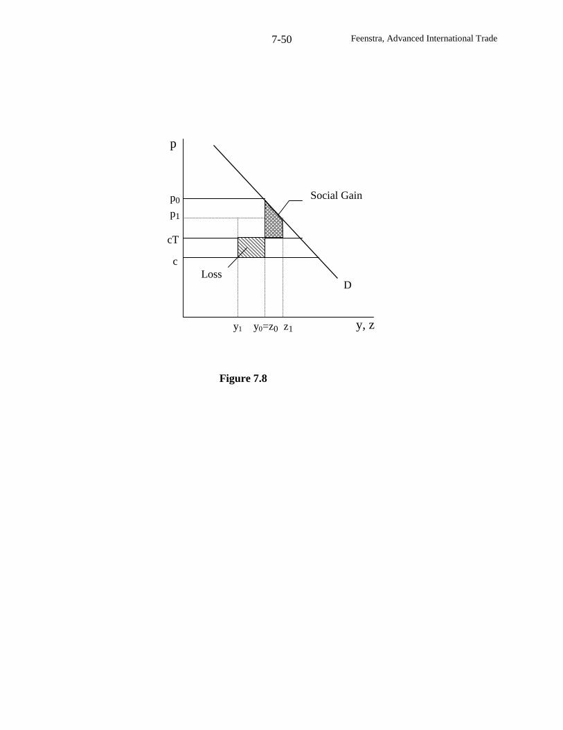
Feenstra, Advanced International Trade7-50
y1 y0=z0 z1
p
p0
p1
cT
c
Social Gain
LossD
y, z
Figure 7.8
Feenstra, Advanced International Trade7-51
foreign firm will indeed sell to the home market.18 Suppose that imports are (z1 – y1), and these
reduce the home price to p1. This brings a rise in global welfare of the area shown (the top
triangle of this area is consumer surplus in the importing country, and the remainder is profits of
the foreign exporter), but a loss in global welfare due to added transport costs shown by the
rectangle. A similar diagram would apply in the foreign country. The relative sizes of these
areas are ambiguous, so we do not know whether trade raises or lowers global welfare.
However, with free entry of firms in both countries, Brander and Krugman argue that
global welfare necessary improves due to free trade. The welfare function with multiple firms is
),NtmL,p(W π++ where π is the profits of each home firm, but with profits equal to zero this
becomes W(p, L + tm). Furthermore, comparing autarky and free trade we have zero tariff
revenue in each case, so welfare is just W(p, L). Thus, welfare will rise going from autarky to
free trade if and only if the import price falls. Brander and Krugman argue that this is indeed
the case: with import competition, prices unambiguously fall, so welfare in both countries
improves. The fall in prices is also reflected in a fall in average costs (since price equals average
costs from zero profits), which implies the output of each firm increases going from autarky to
free trade. So similar to the monopolistic competition model of chapter 5, we have that trade
brings gains due to the exercise of economies of scale. But unlike the monopolistic competition
model, these gains come despite the fact that trade is intrinsically wasteful due to the
homogeneous product and transportation costs.
18 As noted by Brander and Krugman (1983), the condition to observe trade with a single firm in each country is
that the monopoly price, p0 = c η/(η-1) exceeds marginal cost of cT. This is written as η/(η-1) > T, oralternatively, η < T/(T-1). So transport costs cannot be too high relative to the elasticity.
Feenstra, Advanced International Trade7-52
Impact of Anti-Dumping Duties
Suppose that instead of comparing global welfare under free trade and autarky, we
instead consider the effect of an anti-dumping duty imposed by one country. When the number
of firms is fixed at, say, one in each country, this corresponds to the case of Cournot duopoly
analyzed earlier in the chapter. We found there that a small duty was likely to improve the terms
of trade for the importing country, and may also contribute to an efficiency gain through
increasing the output of the home firm. For both reasons, a small tariff was welfare improving
for the importer. Should we think of anti-dumping duties in the same way?
The answer is no. Rather than leading to an improvement in the terms of trade, the
application of anti-dumping law can often lead to a worsening of the terms of trade and a welfare
loss for the importing country. To understand this, we need to review the administration of these
laws in the United States. As discussed by Staiger and Wolak (1994), antidumping actions go
through several distinct phases: an initial investigation by the DOC, which determines whether
or not the imported product is being sold at “less than fair value;” followed by an initial
investigation by the ITC to determine whether or not the domestic industry is “materially
injured;” followed by a final determination of both agencies; followed by the application of
duties if both findings are affirmative and the case is not withdrawn; and then also an annual
administrative review in cases where duties are imposed (Blonigen and Haynes, 2002). Let us
consider how each of these stages affects prices.
Initial Investigation
In the first stage of an investigation, which we call period 1, the DOC compares the
prices of imported products with their prices (or costs) abroad. This calculation involves
comparing the f.o.b. price received by the foreign exporter, which we denote by p1/T, with their
Feenstra, Advanced International Trade7-53
own home price of p*. If p1/T < p* then there is pricing at “less than fair value.” In nearly 95%
of cases brought before the DOC, it concludes that this occurs and recommends duties in period
2 of (1+τ2) = p*/ (p1/T) > 1.
Notice that the duty applied in period 2 depends on the price charged by the exporter in
period 1. In this sense, we must treat the anti-dumping duty as endogenous, and the exporter will
have an incentive to raise its period 1 price so as to lower the period 2 duty.19 Furthermore, this
increase in price occurs even before the duty has been imposed, so that the importing country
does not collect any tariff revenues. This increase in the import price amounts to a pure terms of
trade loss for the importer. Because there is no tariff revenue collected, and still allowing for
free entry of home firms, the welfare criterion is modified from W(p, L + tm) to W(p, L). Thus,
any increase in the import price leads to a welfare loss.
There is evidence that this investigation stage of dumping actions does indeed lead to an
impact on imports, though this is often measured by the effect on quantities rather than prices.
Using a sample of all antidumping cases in the United States from 1980-85, Staiger and Wolak
(1992) find that the initiation of an investigation has a substantial impact on imports, reducing
them by about one-half as much as that would have occurred under duties. The implication is
that import prices must increase, leading to a loss for the importer.
Withdrawal of Cases
While the DOC finds evidence of “pricing at less than fair value” in most cases, the ITC
rules in favor of “material injury” in only about one-half of the cases it considers. Thus, of some
400 cases in the U.S. during 1980-88, about 150 were rejected by the ITC and another 150 had
19 See problems 7.7 and 7.8 to demonstrate this in a model with Bertrand competition.
Feenstra, Advanced International Trade7-54
duties levied. As shown in Table 7.1, the remaining 100 cases or one-quarter of the total were
withdrawn prior to a ruling by the ITC. As described by Prusa (1991, 1992), in these cases the
U.S. firms can negotiate with the foreign firm on the level of prices and market shares. Prusa
finds that withdrawals have about the same impact on reducing import quantity as do actual
duties, which is also found by Staiger and Wolak (1992). Again, the implication is that import
prices would rise, with a direct welfare loss for the importing country.
Continuing Investigations
Consider now the case where an anti-dumping duty has been imposed, and denote the
period 2 import price (inclusive of duty) by p2. Suppose that there is an administrative review to
re-calculate the amount of duty imposed in period 3. In calculating dumping margins during the
administrative review, the DOC removes the tariff from the import price p2, and also removes
any transport costs, obtaining p2/[T(1+τ2)] as the f.o.b. price for the foreign exporter. This is
compared to the exporters home price of p* to determine whether the foreign firm is continuing
in its practice of “pricing at less than fair value.” Whenever p2/[T(1+τ2)] < p* , then duties of
(1+τ3)=p*/[p2/T(1+τ2)] > 1 are imposed in period 3.
Notice that these duties can be re-written as (1+τ3)= (1+τ2)[p*/(p2/T)], so there is a built
in “continuation” of the anti-dumping duties: even if the foreign firm chooses p* = p2/T, so
there would have been no initial evidence of dumping, then it will still be faced with a tariff of
(1+τ3) = (1+τ2) in period 3. In other words, to avoid a charge of continued dumping during the
administrative review, the foreign firm would not only need to increase its period 2 price above
what was charged in period 1, it would need to further increase the period 2 price by the full
Feenstra, Advanced International Trade7-55
amount of the period 2 duty. In the above notation, a charge of dumping is avoided in period 2 if
and only if,
p2/[T(1+τ2)] > p* ⇔ p2 > p* T(1+τ2) > p1(1+τ2), (7.43)
where the last inequality is obtained because dumping occurred in period 1, p1/T < p*.
Using the last inequalities in (7.43), we see that to avoid continuing anti-dumping duties
the import price must rise between period by the amount p2/p1 > (1+τ2), so there is more than
complete pass-through of the period 2 duty. This hypothesis receives strong support from
Blonigen and Haynes (2002). They estimate that the pass-through of the initial anti-dumping
duties can be as high as 160% for the cases that are subject to an administrative review. This
occurs because, as explained above, the DOC removes existing tariffs from import prices when
computing the dumping margin. So in order to avoid duties after an administrative review, the
tariff-inclusive price must rise by more than the amount of duties.
From a welfare point of view, this result very likely violates the criterion for welfare
improvement. With the pass-through of duties exceeding unity, then dp*/dt > 0 so there is a
terms of trade loss. Then the only way that welfare could rise is if there is a large increase in
domestic output with the associated efficiency gain (i.e. if the final term in (7.3) is positive).
However, this source of gain vanishes if there is free entry into the domestic industry so that
profits are zero. In that case, the criterion for welfare gain is (7.26) rather than (7.3), and welfare
can rise only if dp/dt < m/d(p), meaning that the pass-through of the duty is less than the import
share. This is clearly violated when the pass-through is greater than unity. Thus, in all three
stages we have considered – initial investigation, withdrawal of cases, and continuing
investigations – the presumption is that anti-dumping duties will lead to a welfare loss for the
Feenstra, Advanced International Trade7-56
importer. This occurs because the duties being imposed are treated by the exporter as
endogenous, and create an incentive to raise prices so as to avoid the duties.
Conclusions
Since this chapter has covered a large number of different models, a summary is
appropriate. Consider tariffs that are exogenously imposed, such as under the escape clause
provision of the GATT/WTO. In general, this will have three welfare effects on the importing
country: (a) a deadweight loss; (b) a terms of trade effect; (c) a reduction in the monopoly
distortion if the output of home firms increase (without leading to inefficient entry). The
deadweight loss always harms the importer, but is of the second-order of smalls for a small tariff.
The change in the output of home firms, sometimes referred to as a “profit shifting” effect, is of
ambiguous sign and cannot be relied upon to generate gains for the importer. Accordingly, the
best indicator of the welfare impact of small tariffs is the terms of trade effect.
It is sometimes argued that countries must be very large in their sales or purchases of a
product on world markets for their tariff to have an impact on the terms of trade. Even the
United States, it is argued, should be treated as “small” in nearly all markets.20 I disagree with
this assessment. Under imperfect competition, it is quite plausible that foreign exporter will
absorb part of the tariff so the import price does not rise by its full amount; our detailed analysis
of the Cournot and Bertrand cases has identified the exact conditions under which this occurs.
This depends on exporters treating their foreign markets as segmented (i.e. charging different
prices to each), and holds regardless of the size of the importing country. The abundant evidence
on partial pass-through of exchange rates (surveyed in Goldberg and Knetter, 1997) suggests that
20 See Irwin (2002, p. 63).
Feenstra, Advanced International Trade7-57
the same is true for tariffs, though the exact magnitude of pass-through will depend on the
industry being considered. For the comparison of the U.S. tariffs on truck and motorcycles we
found quite different pass-through behavior, with the tariff on trucks generating a terms of trade
gain but not the tariff on motorcycles.
Even if we accept that in many industries there will be a terms of trade and welfare gain
due to a small tariff, this hardly justifies their use: the terms of trade gain comes entirely at the
expense of foreign exports, so this is a “beggar thy neighbor” policy. The use of tariffs can
therefore invite retaliation from trading partners. A very recent example of this has occurred in
the steel industry in the U.S., which received Section 201 protection in March 2002.21 Declining
tariffs ranging from 8% to 30% were applied for three years to a range of steel products and
various importers.22 Shortly after these tariffs were imposed the European Union, Japan, and
Korea announced plans to file protests with the WTO, and retaliate with tariffs of their own
applied against U.S. products. Such retaliation means that the use of tariffs becomes a negative
sum game, i.e. they can end up harming both trading partners.
What can prevent a country from attempting to move the terms of trade in its favor? One
view of the GATT is that it was designed with exactly this goal in mind. Bagwell and Staiger
(1999, 2002) argue that the provisions of GATT such as “reciprocity” (i.e. tariff reductions
should be reciprocal across countries) are effective in preventing countries from using tariffs to
improve their terms of trade. We will discuss this further in chapter 9. By a similar logic, I think
that the escape clause provision of the GATT should be viewed as a way to promote free trade
21 This was the first instance of a Section 201 action that was initiated by the President (and followed from acampaign promise made by George W. Bush while campaigning in steel producing states).22 Some of the tariffs took the form of “tariff-rate quotas,” which means that the tariffs are applied only for importsfrom each source country in excess of some amount. These quotas can be varied preferentially across sourcecountries without violated the MFN principle of the GATT. Canada, Mexico, Israel and Jordan are entirely exemptfrom the tariffs because of their free trade agreements with the United States.
Feenstra, Advanced International Trade7-58
while allowing for exceptions in specific circumstances. The linkage was made explicit in the
recent Section 201 protection to the steel industry in the U.S., where the Bush administration
hoped to secure additional votes for “fast track” authority.23 So Article XIX of the GATT and
Section 201 of U.S. trade law need to be assessed in a broader political-economy context of
securing industry support for free trade. Given that these provisions are used rarely, and only
temporarily, they can be viewed as rather effective.
The same is not true of the anti-dumping provisions of GATT. As we have argued, the
GATT definition of dumping will apply in many markets subject to imperfect competition, and
there has been an increasingly widespread use of the dumping provisions. The anti-dumping
duties that are imposed must be treated as endogenous: they depend on the prices chosen by the
exporter prior to, and during, the dumping action. This creates an incentive for exporter to raise
their prices before dumping duties are imposed, and to raise them even further before an
administrative review of the dumping case. These actions correspond to a terms of trade loss for
the importer, as indicated by the empirical evidence of Blonigen and Haynes (2002). This can
also be reflected in an increase in the price of import-competing products, of course, so the anti-
dumping duties act so as to promote more collusive behavior. Gallaway, et al (1999) estimate
the combined welfare cost of anti-dumping and countervailing duty legislation in the U.S. to be
some $4 billion in 1993. In the next chapter, we will also find that import quotas can lead to
more collusive behavior among firms, so that along with anti-dumping legislation, these must be
judged as very costly policies.
23 “Fast track” authority refers to the ability of the executive branch to present to the U.S. Congress a proposal foran expansion of free trade, for an “up or down” vote without allowing amendments. This authority is used, forexample, when negotiating free trade areas, which the Bush administration intends to pursue in the Americas. Fasttrack authority was renewed by the U.S. House of Representatives in July 2002, by a narrow vote in favor.
Feenstra, Advanced International Trade7-59
Problems
7.1 Derive the optimal specific tariff from (7.12) in the case where there is a single foreign firm,
and the demand curve d(p) is linear.
7.2 Derive conditions under which the Cournot reaction curves in Figure 7.4 are both downward
sloping.
7.3 By totally differentiating the equilibrium condition (7.22), show that:
(a) dy/dt > 0 provided that 0)yx("yp)yx('p <+++ ;
(b) The total change in home profits πdue to the tariff is positive.
7.4 In this problem we derive the properties of the elasticities used with Bertrand competition.
(a) First review problem 1.2 of chapter 1, and show that if a function y = f(v) is homogeneous
of degree α, meaning that for all λ > 0, f(λv) = λα f(v), then its first derivative is homogeneous of
degree α-1.
(b) Thus, if demand d(p,q,I) is homogeneous of degree zero in (p,q,I), then dq(p,q,I) is
homogeneous of degree minus one. Use this to show that η(p,q,I) = qdq(p,q,I)/d(p,q,I) is
homogeneous of degree zero in (p,q,I).
(c) Now assume that the income elasticity is unity, so that demand is written as d(p,q,I) =
φ(p,q)I. Show that the elasticity η does not depend on I. Therefore, show that the elasticity η
can be written as a function of q/p.
Feenstra, Advanced International Trade7-60
7.5 Using the results from problem 7.4, assume that 0)q/p(*' >η and 0)p/q(' >η .
(a) Then by differentiating the first-order conditions (7.28), show that the reaction curves p =
r*(q,τ) and q = r(p) both slope upwards, as shown in Figure 7.6, with elasticities less than
unity.
(b) Also compute the elasticity of the foreign reaction curve p = r*(q, τ) with respect to τ.
(c) Use the results in (a) and (b) to solve for the total change in q and p due to the tariff.
7.6 (a) Output of the home firm is y = d(q,p,I). Use the fact that d(q,p,I) is homogeneous of
degree zero in (q,p,I) to show that dqq + dpp + dII = 0. Then use the assumption that the income
elasticity of demand is unity to show that dpp/d = (η–1).
(b) Using (a), compute the total change in home output y = d(q,p,I) as p increases along the home
reaction curve. Show that output increases if 0 < 2)1(p/'q −η<ηη .
7.7 Under Bertrand competition, show that foreign profits fall due to the tariff when
0)q/p(*' >η and 0)p/q(' >η .
7.8 Consider the problem of an exporting firm facing the threat of an anti-dumping duty. Given
the period 1 import price chosen by the exporting firm, the duty imposed in period 2 equals
(1+τ2) = p*/p1 whenever p1 < p*. This tariff is imposed with probability θ, and conversely, with
probability (1-θ) there will be no duty. Denote the value of period 2 profits when the duty is
imposed by )( 2*2 τπ , where from problem 7.7 we have that 0)(' 2
*2 <τπ . Let )0(*
2π denote the
maximized value of period 2 profits for the foreign firm in the case of zero duty. Then the
period 1 problem can be stated as:
Feenstra, Advanced International Trade7-61
12*22
*211
pp/*p)1(.t.s)]0()1()([)q,p(*max
1
=τ+πθ−+τθπδ+π . (7.44)
We suppose that the home firm chooses q1, under Bertrand competition. Derive the first-order
conditions for the home and foreign firms, and show that the threatened duty leads to an increase
in the foreign price p1.
Feenstra, Advanced International Trade7-62
Empirical Exercise
In this exercise, you are asked to reproduce some of the empirical results from Feenstra (1989).
To complete the exercise, the files “cars.csv, trucks.csv, cycon.csv, cyship.csv, cypool.csv”
should be stored in the directory: c:\Empirical_Exercise\Chapter_7\. Each of these can be used
in STATA programs “cars.do, trucks.do, cycon.do, cyship.do, cypool.do”
to create a dataset with the variables described in “Documentation_Chp7.doc.” Use these “do”
programs to answer the following:
7.1 Replicate Table 7.2, i.e., run the specifications of (7.34) without imposing the tests of
symmetry or homogeneity. Duplicate all of the coefficients that are reported in this table, except
the Durbin-Watson statistics.
7.2 Then replicate Feenstra’s Table 7.2 by imposing the tests of homogeneity and symmetry,
shown in (7.35a) and (7.35b). Instead of conducting the Wald test, as done in Feenstra (1989),
instead conduct the analogous F-test. Do you accept or reject the hypotheses of symmetry and
homogeneity?

Feenstra, Advanced International Trade
Chapter 8: Import Quotas and Export Subsidies
In addition to import tariffs, quotas and subsidies are widely used forms of trade policy.
Quotas and subsidies can in principle be applied to either imports or exports, but we will focus
here on import quotas and export subsidies. How do these policy instruments differ from tariffs,
and does this depend on the type of competition in the market? These are the questions we shall
investigate in this chapter.
We begin with the result of Bhagwati (1965) on the “equivalence” of tariffs and quotas.
This means that under perfect competition, applying a quota that limits the number of units
imported will have essentially the same effects as applying a certain level of tariff: for each
quota, there is an “equivalent” tariff. This equivalence result no longer holds under imperfect
competition, however. Bhagwati (1965) considered a monopolistic home importer subject to a
quota, and that analysis was later extended to duopoly with a home firm and foreign firm subject
to an import quota (Harris, 1985, Krishna, 1989). As we shall see, a quota and tariff that have
comparable effects on the level of imports can then have quite different effects on the import
price, and therefore on welfare in the importing country.
Another reason for tariffs and quotas to differ occurs when foreign firms can choose the
quality of the good that they export. In that case, a limitation on the number of units exported (as
under a quota) will have quite a different impact from a tariff on the value of exports (as with an
ad valorem tariff). The importance of this case became apparent with the quota applied to
Japanese auto exports to the United States during the 1980s. The evidence strongly supports the
hypothesis that Japanese firms changed the characteristics of the cars they sold, shifting towards
higher quality and higher-priced models. We shall describe a theoretical model of quality choice
and the empirical evidence for autos (Feenstra, 1988a).

Feenstra, Advanced International Trade8-2
The finding that trade policies have differing effects depending on the market structure
carries over to the case of export subsidies. In the conventional two-sector model, there is no
reason to use export subsidies: they will lead to a deadweight loss (analogous to a tariff) for a
small country, and have an additional terms of trade loss (the opposite of a tariff) for a large
country. This seems to contradict the fact that many countries have used export subsidies to
support their industries at some time. To explain this, we need to go beyond the two-sector
model with perfect competition. Adding more goods turns out to make a difference, and there is
a potential role for targeted export subsidies in models with many goods (Feenstra, 1986, Itoh
and Kiyono, 1987).
Dropping perfect competition, and instead allowing for duopoly between a home and
foreign firm exporting to a third market, also makes a difference. The question then is whether
the home government can give its own firm a “strategic” advantage by subsidizing it. We shall
require that the subsidy also be in the national interest, which means that profits for the exporter
need to rise by more than the amount of the subsidy itself. Initial analysis of this problem
(Brander and Spencer, 1985) suggested that such an advantage would indeed occur, at least
under Cournot-Nash competition. Later work, however (Eaton and Grossman, 1986), showed
that this advantage would be reversed under Bertrand competition. The conclusion is that export
subsidies are in the national interest only under some forms of market competition, but not
generally. We conclude the chapter by investigating the effects of subsidies to the production of
commercial aircraft, produced by Boeing in America and Airbus in Europe. Irwin and Pavcnik
(2001) have recently investigated the effects of subsidies on prices and profits in this industry, as
we shall discuss.
Feenstra, Advanced International Trade8-3
Equivalence of Tariffs and Quotas
The analysis of quotas under perfect competition proceeds much like our graphical
treatment of tariffs, in the previous chapter. In panel (a) of Figure 8.1 we show the domestic
demand D and supply curve S, together with the constant world price p*. Under free trade,
domestic demand is at c0 and supply at y0, so imports are m0 = c0 – y0. The import demand
curve M = D – S is shown in panel (b), together with the horizontal export supply curve X at the
world price p*. These intersect at the equilibrium imports m0.
Now suppose that an import quota of X is imposed, meaning that the quantity imported
cannot exceed this amount. This effectively established a vertical export supply curve denoted
by X in panel (b), which now intersects import demand at m1 with the price of p1. In panel (a),
the price of p1 leads to increased supply of y1 and reduced demand of d1. Notice that there
would be an equivalent effect on price, consumption and production if instead the government
had imposed a tariff of t ≡ p1 – p0. In this sense, for every quota there is an equivalent tariff.
The welfare change from having the quota in Figure 8.1 is: –(a+b+c+d) consumer surplus
loss +(a) producer surplus gain. However, the area (c), which would be collected as revenue
under a tariff, now needs to be considered more carefully. This area is the difference between
the domestic price p1 and the world price p*. Therefore, whoever is actually importing the good
stands to collect the pure profits or “rents” equal to (p1 – p*)m1, which is area (c). There are four
possible ways that these quota rents can be allocated.
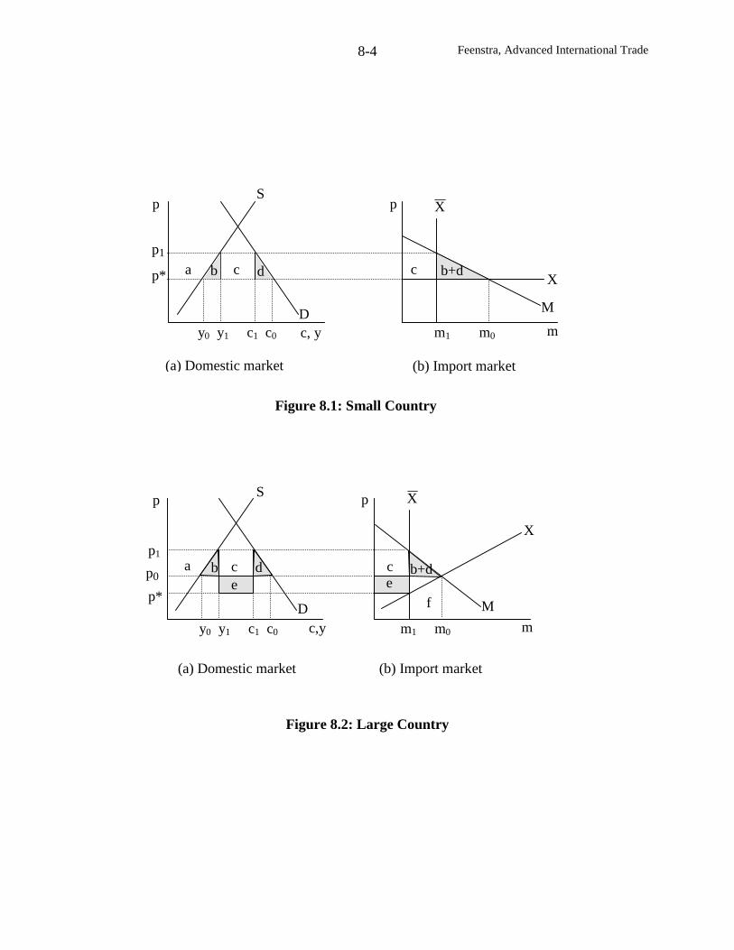
Feenstra, Advanced International Trade8-4
a c
y0 y1 c1 c0
(a) Domestic market
c
Figure 8.1: Small Country
D
p1
p*
p
c, y
S
db
p
mm1 m0
(b) Import market
X
M
X
b+d
p
m
e
D
p
a
c,y
cp1
p0
p*
y0 y1 c1 c0
S
b d
m1 m0
M
X
eb+d
(a) Domestic market (b) Import market
Figure 8.2: Large Country
X
c
f
Feenstra, Advanced International Trade8-5
First, the quota licenses can be given to home firms, who are then able to import at the
world price p* and sell domestically at p1, earning the difference between these as rents. An
example of this is the dairy industry in the United States, where U.S. producers of cheese also
receive licenses to import from abroad.1 With home firms earning the rents c, the net loss in
domestic welfare due to the quota is –(a+b+c+d) consumer surplus loss +(a+c) producer surplus
gain = –(b+d), which is the same loss as we found for a tariff.
However, a second possibility is that while the quota licenses are given to home firms,
these firms engage in some kind of inefficient activities in order to obtain the licenses. For
example, if licenses for some imported input are allocate in proportion to the previous year’s
production of a final good, then firms will produce more final goods than they can sell (and
probably of lower quality) just to obtain the import licenses. Krueger (1974) called this kind of
activity “rent seeking,” and it can include lobbying and other resource-using activities. It has
been suggested that the waste of resources devoted to rent seeking activities could be as large as
the value of rents themselves, so that the area (c) would be wasted rather than accrue to domestic
firms. In that case, the welfare loss due to the quota would be –(a+b+c+d) consumer surplus loss
+(a) producer surplus gain = –(b+d+c), which is greater than for the tariff.2
Third, the quota licenses can be auctioned by the government of the importing country.
This has occurred in New Zealand, for example.3 In a well-organized auction, we might expect
that the revenue collected would equal the value of the rents, so that area (c) accrues to the home
government. In that case, the net loss in domestic welfare due to the quota is –(a+b+c+d)
1 As described in Hornig, et al (1990), there is some sharing of the quotas rents between importers and exporters.2 Bhagwati and Srinivasan (1980) have suggested, however, that there might also be “profit-seeking” activities fortariff revenue, in which case we ought to take this into account for a tariff, too.3 See Bergsten, et al (1987).
Feenstra, Advanced International Trade8-6
consumer surplus loss +(a) producer surplus gain +(c) auction revenue = –(b+d), which is again
the same loss as we found for a tariff.
Finally, the government of the importing country can give authority for implementing the
quota to the government of the exporting country. Because the exporting country allocates the
quota among its own producers, this is sometimes called a “voluntary” export restraint (VER), or
“voluntary” restraint agreements (VRA). This arrangement has occurred for quotas that the
United States has used in automobiles, steel, textiles, and other industries. In automobile imports
for Japan after 1981, for example, the Ministry of International Trade and Industry (MITI) told
each auto manufacturer in Japan how much it could export to the U.S. We have discussed the
background to this case in the previous chapter, and will analyze it in detail later in this chapter.
At this point, we note that the quota rents are then earned by foreign producers, so the loss in
domestic welfare equals: –(a+b+c+d) consumer surplus loss +(a) producer surplus gain =
–(b+d+c), which is larger than for a tariff.4
In Figure 8.2 we extend the analysis of the quota to a large country. In that case the
quota rents might be measured as (c) or (c+e), and these accrue to the foreign producers under a
VER. The deadweight loss for the importing country is still measured by area (b+d), and it can
be argued that the area (f) represents an analogous deadweight loss for the foreign country . In
Table 8.1 we present some estimates of the home and foreign deadweight loss, along with the
rents, for major U.S. quotas around 1985. In all cases except diary, these rents were earned by
foreign exporters. We will be discussing the case of automobiles later in the chapter, and
estimates of the quota rents earned by foreigners range from $2 to 8 billion. Textiles and apparel
4 This raises the question of why a country would use a VER since it gives the rents to foreigners. One answer isthat this helps to prevent retaliation by the foreign countries. In addition, Feenstra and Lewis (1991b) argue thattransferring the rents to foreigners serves as an “incentive compatibility” device, so that the importing country willonly use the VER if the domestic industry is genuinely harmed.
Feenstra, Advanced International Trade8-7
Table 8.1: Annual Cost of U.S. Import Protection(billion dollars, years around 1985)
U.S. Deadweight Loss(area b + d)
Quota rents(c or c+e)
Foreign DeadweightLoss (area f)
Automobiles 0.2 – 1.2 2.2 – 7.9 0 – 3
Dairy 1.4 0.25 0.02
Steel 0.1 – 0.3 0.7 – 2.0 0.1
Sugar 0.1 0.4 – 1.3 0.2
Textiles and Apparel 4.9 – 5.9 4.0 – 6.1 4 – 15.5
Average Tariffs 1.2 – 3.4 0__ n.a.__
Total* 7.9 – 12.3 7.3 – 17.3 4.3 – 18.8
Source: Feenstra (1992), with detailed sources cited there.
Notes:
* In dairy the quota rents are earned by U.S. importers, and so are not included in the total.n.a. – not available
Feenstra, Advanced International Trade8-8
also have very large quota rents and U.S. deadweight losses (about $5 billion each), under the
global system of quotas known as the Multi-Fiber Arrangement (MFA). The foreign deadweight
losses due the MFA are even larger, with estimates ranging from $4 to $16 billion. The upper
end of these estimates is obtained from models that include very costly rent-seeking activities by
foreign producers in developing countries.
Summing the costs shown in Table 8.1, the total deadweight loss due to these quotas is in
the range of $8 to $12 billion annually in the mid-1980s, while the quota rents transferred to
foreigners are another $7 to $17 billion annually. Some of these costs for the U.S. are no longer
relevant today: the quota in automobiles ceased to be binding after 1987, as discussed later in
the chapter, and under the Uruguay Round of the WTO it was agreed that the MFA would be
dismantled. But that action is being delayed until 2005, and even for automobiles, there is
always the possibility of new trade actions.5 The quotas in the steel industry whose costs are
summarized in Table 8.1 have been recently replaced by tariffs, instead (as described at the end
of chapter 7). In addition, the “average tariffs” included in the last row of Table 8.1 reflect only
conventional tariffs, and does not include the additional cost due to U.S. anti-dumping duties
(estimated as some $4 billion annually, also discussed at the end of chapter 7). In summary, the
quotas and tariffs/duties used by the U.S. continue to impose a significant cost on itself and on
foreign trading partners.
Non-Equivalence due to Imperfect Competition
We have shown above the equivalence of tariffs and quotas, in the sense that when each
instrument is chosen to have the same import level, then it also has the same impact on prices.
When there is imperfect competition in the domestic market, however, this result quickly breaks
5 See Levinsohn (1997), who discusses a 1995 trade dispute in autos between the U.S. and Japan.
Feenstra, Advanced International Trade8-9
down. The reason is that the quota creates a “sheltered” market for the domestic firm, which will
lead to higher prices and lower sales than under a tariff with same level of imports. For the case
of a domestic monopoly, as analyzed by Bhagwati (1965), this is demonstrated in Figure 8.3.
With the fixed world price of p*, the demand curve facing the domestic monopolist is
essentially horizontal at that price, so marginal revenue is also horizontal and the profit-
maximizing quantity is y0, where marginal revenue equals marginal cost. Note that this is the
same quantity that a competitive firm or industry would produce if it had the same marginal costs
as the monopolist. In this sense, free trade in a small country eliminates the market power of the
monopolist, i.e. eliminates its ability to restrict supply and raise price. This is a potential extra
source of gains from trade.
Suppose initially that a tariff of t is applied to imports. In that case, the domestic
monopolist can charge as much as p* + t, but no more, so its demand curve is now horizontal at
that price. This means that its marginal revenue curve is also horizontal at p* + t, so the profit-
maximizing quantity is where that price equals marginal cost, which is y1 in Figure 8.3.
Consumption at that price is c1, so imports are m1 = c1 – y1.
Now suppose that instead of the tariff, a quota of m1 is applied. This means that for any
price above p*, the fixed amount m1 will be imported, so the demand curve facing the
monopolist is the initial demand curve D less the amount m1, which we illustrate by D – M1.
Unlike the situation under the tariff, the monopolist retains the ability to influence the domestic
price: it can choose the optimal price and quantity along D – M1. So we graph the marginal
revenue curve below D – M1, which is denoted by MR, and find the profit-maximizing price and
Feenstra, Advanced International Trade8-10
quantity where this intersects marginal cost, at p2 and y2. It will definitely be the case that p2 >
p*+t, so that the quota with the same level of imports as the tariff has led to a higher domestic
price. Therefore, the tariff and quota are no longer equivalent: the quota enables the monopolist
to exercise market power, and has a higher welfare cost for this reason.
It is also the case that the quota might even lead to a fall in domestic output as compared
to free trade. This is illustrated in Figure 8.3 by y2 < y0. This is not a necessary result, and we
could instead have drawn the MR curve so that y2 > y0. It is rather surprising that y2 < y0 is even
possible, because it suggests that workers in the industry would fail to be protected by the quota:
that is, employment could fall due to the reduction in output under the quota. We see, then, that
this policy instrument has quite undesirable results as compared to a tariff.
These results of Bhagwati (1965) give us good insight into the effect of a tariff versus a
quota under imperfect competition, but the assumption that the domestic monopoly does not
interact at all with foreign firms is not satisfactory. Presumably, the domestic firm would be
competing with foreign firms, under Cournot or Bertrand competition. In the first case,
Cournot-Nash competition, the import quota has rather predictable effects: restricting the
foreign firms to sell less than its free trade amount will shift sales towards the domestic firm,
under the normal shape of reaction curves.6 In order to obtain more dramatic results, we instead
consider an import quota (restricting quantity) in a game where the two firms are initially
engaged in Bertrand competition (taking each other’s prices as given). This case has been
analyzed by Harris (1985) and Krishna (1989), and we follow the exposition of Harris.
As in the previous chapter, we assume that the imported and domestic products are
6 See problem 8.1.
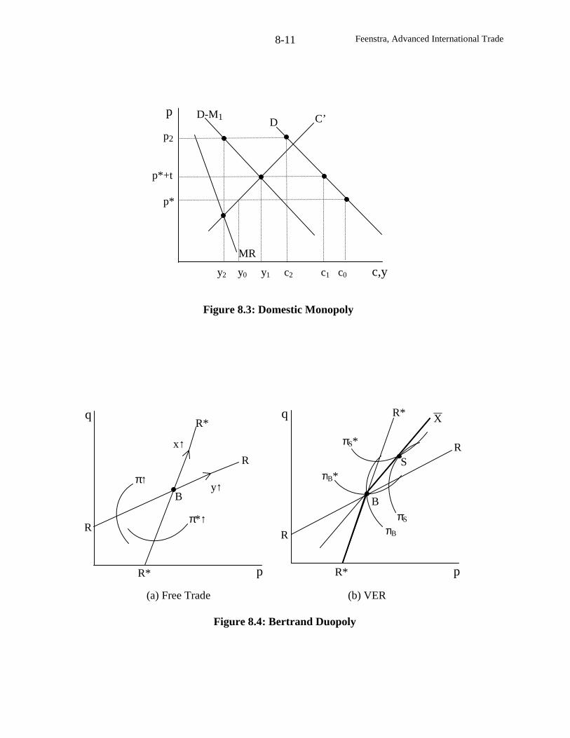
Feenstra, Advanced International Trade8-11
p
MR
p2
p*+t
p*
y2 y0 y1 c2 c1 c0 c,y
C’DD-M1
Figure 8.3: Domestic Monopoly
R
q
pR*
π↑B
x↑R
R*
y↑
π*↑
(a) Free Trade (b) VER
Figure 8.4: Bertrand Duopoly
πS*
πB*
πB
πS
S
B
R
q
R* p
R*
R
X
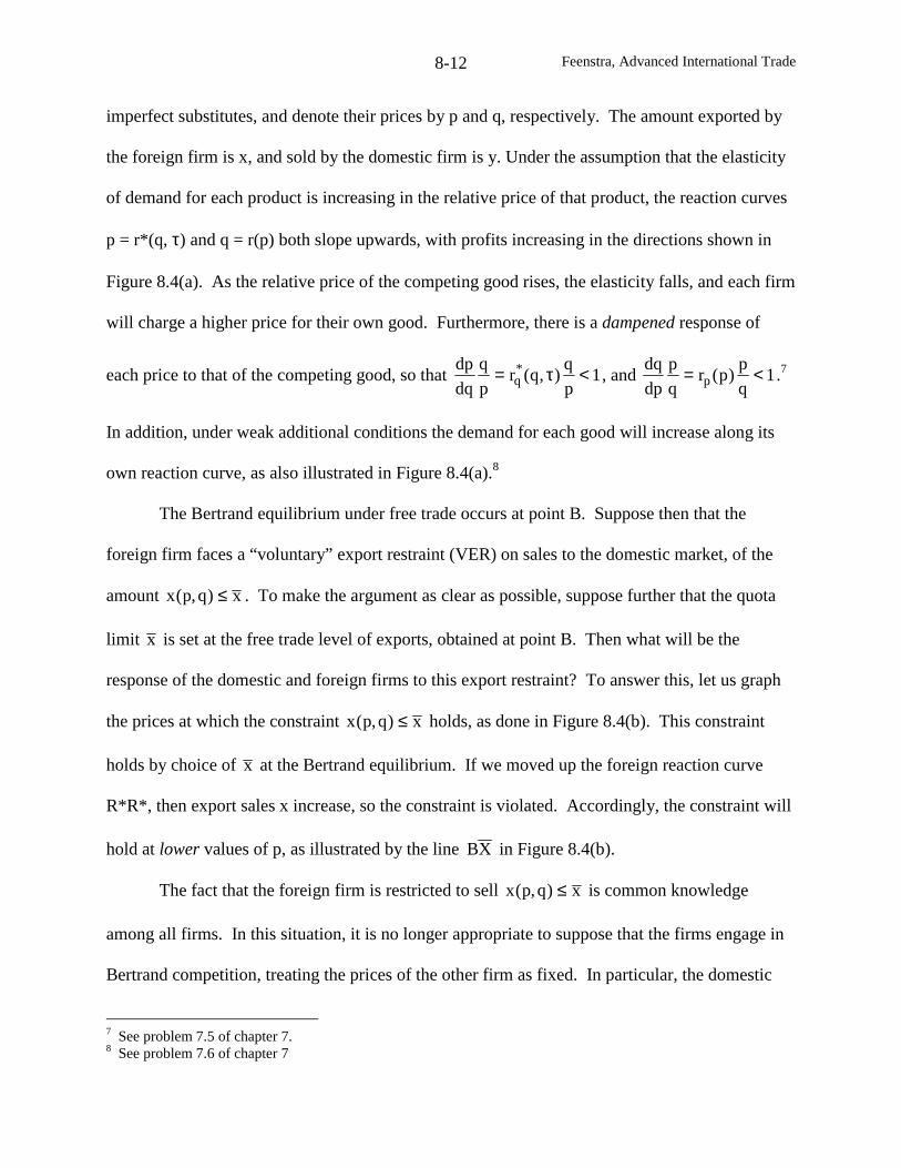
Feenstra, Advanced International Trade8-12
imperfect substitutes, and denote their prices by p and q, respectively. The amount exported by
the foreign firm is x, and sold by the domestic firm is y. Under the assumption that the elasticity
of demand for each product is increasing in the relative price of that product, the reaction curves
p = r*(q, τ) and q = r(p) both slope upwards, with profits increasing in the directions shown in
Figure 8.4(a). As the relative price of the competing good rises, the elasticity falls, and each firm
will charge a higher price for their own good. Furthermore, there is a dampened response of
each price to that of the competing good, so that 1p
q),q(r
p
q
dq
dp *q <τ= , and 1
q
p)p(r
q
p
dp
dqp <= .7
In addition, under weak additional conditions the demand for each good will increase along its
own reaction curve, as also illustrated in Figure 8.4(a).8
The Bertrand equilibrium under free trade occurs at point B. Suppose then that the
foreign firm faces a “voluntary” export restraint (VER) on sales to the domestic market, of the
amount x)q,p(x ≤ . To make the argument as clear as possible, suppose further that the quota
limit x is set at the free trade level of exports, obtained at point B. Then what will be the
response of the domestic and foreign firms to this export restraint? To answer this, let us graph
the prices at which the constraint x)q,p(x ≤ holds, as done in Figure 8.4(b). This constraint
holds by choice of x at the Bertrand equilibrium. If we moved up the foreign reaction curve
R*R*, then export sales x increase, so the constraint is violated. Accordingly, the constraint will
hold at lower values of p, as illustrated by the line XB in Figure 8.4(b).
The fact that the foreign firm is restricted to sell x)q,p(x ≤ is common knowledge
among all firms. In this situation, it is no longer appropriate to suppose that the firms engage in
Bertrand competition, treating the prices of the other firm as fixed. In particular, the domestic
7 See problem 7.5 of chapter 7.8 See problem 7.6 of chapter 7
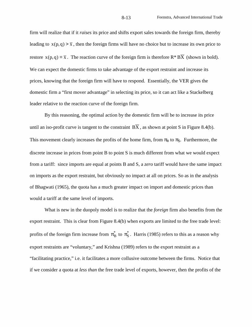
Feenstra, Advanced International Trade8-13
firm will realize that if it raises its price and shifts export sales towards the foreign firm, thereby
leading to x)q,p(x > , then the foreign firms will have no choice but to increase its own price to
restore x)q,p(x = . The reaction curve of the foreign firm is therefore R* XB (shown in bold).
We can expect the domestic firms to take advantage of the export restraint and increase its
prices, knowing that the foreign firm will have to respond. Essentially, the VER gives the
domestic firm a “first mover advantage” in selecting its price, so it can act like a Stackelberg
leader relative to the reaction curve of the foreign firm.
By this reasoning, the optimal action by the domestic firm will be to increase its price
until an iso-profit curve is tangent to the constraint XB , as shown at point S in Figure 8.4(b).
This movement clearly increases the profits of the home firm, from πB to πS. Furthermore, the
discrete increase in prices from point B to point S is much different from what we would expect
from a tariff: since imports are equal at points B and S, a zero tariff would have the same impact
on imports as the export restraint, but obviously no impact at all on prices. So as in the analysis
of Bhagwati (1965), the quota has a much greater impact on import and domestic prices than
would a tariff at the same level of imports.
What is new in the duopoly model is to realize that the foreign firm also benefits from the
export restraint. This is clear from Figure 8.4(b) when exports are limited to the free trade level:
profits of the foreign firm increase from *Bπ to *
Sπ . Harris (1985) refers to this as a reason why
export restraints are “voluntary,” and Krishna (1989) refers to the export restraint as a
“facilitating practice,” i.e. it facilitates a more collusive outcome between the firms. Notice that
if we consider a quota at less than the free trade level of exports, however, then the profits of the
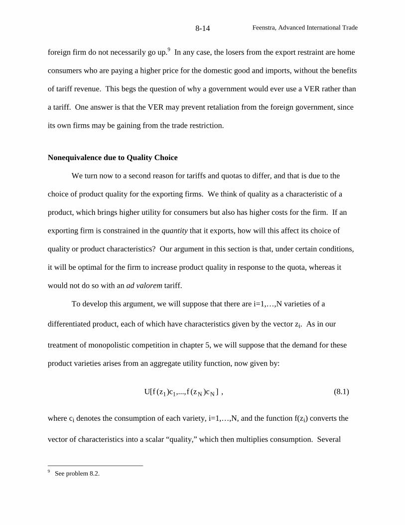
Feenstra, Advanced International Trade8-14
foreign firm do not necessarily go up.9 In any case, the losers from the export restraint are home
consumers who are paying a higher price for the domestic good and imports, without the benefits
of tariff revenue. This begs the question of why a government would ever use a VER rather than
a tariff. One answer is that the VER may prevent retaliation from the foreign government, since
its own firms may be gaining from the trade restriction.
Nonequivalence due to Quality Choice
We turn now to a second reason for tariffs and quotas to differ, and that is due to the
choice of product quality for the exporting firms. We think of quality as a characteristic of a
product, which brings higher utility for consumers but also has higher costs for the firm. If an
exporting firm is constrained in the quantity that it exports, how will this affect its choice of
quality or product characteristics? Our argument in this section is that, under certain conditions,
it will be optimal for the firm to increase product quality in response to the quota, whereas it
would not do so with an ad valorem tariff.
To develop this argument, we will suppose that there are i=1,…,N varieties of a
differentiated product, each of which have characteristics given by the vector zi. As in our
treatment of monopolistic competition in chapter 5, we will suppose that the demand for these
product varieties arises from an aggregate utility function, now given by:
]c)z(f,...,c)z(f[U NN11 , (8.1)
where ci denotes the consumption of each variety, i=1,…,N, and the function f(zi) converts the
vector of characteristics into a scalar “quality,” which then multiplies consumption. Several
9 See problem 8.2.
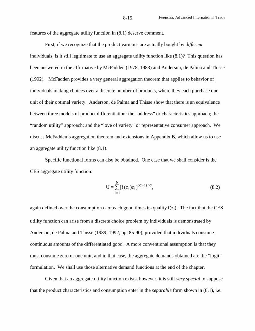
Feenstra, Advanced International Trade8-15
features of the aggregate utility function in (8.1) deserve comment.
First, if we recognize that the product varieties are actually bought by different
individuals, is it still legitimate to use an aggregate utility function like (8.1)? This question has
been answered in the affirmative by McFadden (1978, 1983) and Anderson, de Palma and Thisse
(1992). McFadden provides a very general aggregation theorem that applies to behavior of
individuals making choices over a discrete number of products, where they each purchase one
unit of their optimal variety. Anderson, de Palma and Thisse show that there is an equivalence
between three models of product differentiation: the “address” or characteristics approach; the
“random utility” approach; and the “love of variety” or representative consumer approach. We
discuss McFadden’s aggregation theorem and extensions in Appendix B, which allow us to use
an aggregate utility function like (8.1).
Specific functional forms can also be obtained. One case that we shall consider is the
CES aggregate utility function:
∑=
σ−σ=N
1i
/)1(ii ,]c)z(f[U (8.2)
again defined over the consumption ci of each good times its quality f(zi). The fact that the CES
utility function can arise from a discrete choice problem by individuals is demonstrated by
Anderson, de Palma and Thisse (1989; 1992, pp. 85-90), provided that individuals consume
continuous amounts of the differentiated good. A more conventional assumption is that they
must consume zero or one unit, and in that case, the aggregate demands obtained are the “logit”
formulation. We shall use those alternative demand functions at the end of the chapter.
Given that an aggregate utility function exists, however, it is still very special to suppose
that the product characteristics and consumption enter in the separable form shown in (8.1), i.e.
Feenstra, Advanced International Trade8-16
in the form f(zi)ci, which we can interpret as “quality times quantity.” This functional form
implies that every unit consumed of good i is evaluated at the same quality. This form of the
utility function was used by Swan (1970), but criticized as being too special by Spence (1975).
Spence uses the more general formulation φ(zi, ci), under which the marginal utility of
characteristics per unit consumed, φz(zi, ci)/ci, can vary with the level of consumption ci. If we
interpret demand as coming from different individuals, then φz(zi, ci)/ci depending on ci means
that consumers have differing valuations of characteristics. We will use the special form f(zi)ci
for convenience, but as we shall repeatedly emphasize, the results that we obtain on quality
upgrading will not necessarily carry over to more general functional forms.
Free Trade Equilibrium
We begin by analyzing the problem for consumers and firms in the absence of any quota
restriction. Consumers are presented with a set of i=1,…,N varieties, with fixed characteristics zi
and prices pi, and then choose the optimal quantity of each variety. It will be convenient to work
with the “quality adjusted” prices, which are defined by qi ≡ pi/f(zi). That is, the higher is overall
product quality f(zi), the lower are the quality-adjusted prices qi. The aggregate consumer
maximizes utility in (8.1), subject to the budget constraint ∑ = ≤N1i ii Icp . The Lagrangian for
this problem is,
)cpI(]c)z(f,...,c)z(f[UL iN
1i iNN11 ∑ =−λ+=
)dqI()d,...,d(U iN
1i iN1 ∑ =−λ+= , (8.3)
Feenstra, Advanced International Trade8-17
where the second line of (8.3) follows by defining di ≡ f(zi)ci as the effective “quality-adjusted”
demand, and also using the quality-adjusted prices qi ≡ pi/f(zi). This re-writing of the
Lagrangian makes it clear that instead of choosing ci given prices pi and characteristics zi, we
can instead think of the aggregate consumer as choosing di given quality-adjusted prices qi,
i=1,…,N. Let us denote the solution to problem (8.3) by di(q, I), where q is the vector of quality-
adjusted prices.
Varieties of the differentiated product can be sold by domestic and foreign firms, which
we do not distinguish in the notation. Producing one unit of product i with characteristics zi
requires unit-costs of gi(zi), where we are treating factor prices as constant and suppress them in
this cost function.10 For simplicity, we are assuming constant returns to scale, so that the costs
g(zi) do not depend on the level of output. Firms simultaneously choose prices pi and
characteristics zi, for the i=1,…,N varieties. Suppose that a given firm produces the first
i=1,…,M product varieties. Consumption of each of these is ci = di(q, I)/f(zi). The profit-
maximization problem for this firm is then:
∑∑==
−=−
M
1ii
i
iiiz,q
maxM
1iiiiiz,p
max)I,q(d
)z(f
)z(gqc)]z(gp[
iiii. (8.4)
Again, we have changed the variables from nominal prices pi to quality-adjusted prices qi when
10 We index the function gi(zi) by i to reflect that firms might have access to different technologies. This will leadthem to products with different characteristics in equilibrium.
Feenstra, Advanced International Trade8-18
moving from the left to the right of (8.4). This transformation relies on our assumption that
prices and characteristics are chosen simultaneously, as well as our special functional forms.
It is immediate that to maximize profits in (8.4), the firms must minimize gi(zi)/f(zi),
which is interpreted as the costs per unit of quality for good i. Taking logs and minimizing this
over the choice of characteristics zi leads to the first-order conditions,
i
i
iiii z
g
)z(g
1
z
f
)z(f
1
∂∂=
∂∂
, i=1,…,M. (8.5)
Thus, we obtain equality between the relative marginal utility from each characteristic, on the
left of (8.5), and its relative marginal cost, on the right. Notice that this condition holds despite
the fact that the firm will be choosing its prices in a monopolistically competitive fashion,
provided the prices and characteristics are chosen simultaneously.11
Maximizing (8.5) over the choice of prices pi, we obtain the first-order conditions,
0q
d
)z(f
)z(gq)I,q(d
M
1j i
j
j
jjji =
∂∂
−+∑
=, i=1,…,M. (8.6)
This expression is slightly more complicated than usual because the firm is selling multiple
products j=1,…,M, and therefore must take into account the effect of a change in price qi on all
these products. To simplify this, let us consider the case of a CES utility function in (8.2). Then
11 It is well known that a condition like (8.5) holds in a competitive market (as described in the classic article byRosen, 1974) and Swan (1970) first showed that it holds under monopoly as well, using the special functional formswe have assumed. When prices and characteristics are not chosen simultaneously, then we do not obtain theequality shown in (8.5); see Feenstra (1995), for example.
Feenstra, Advanced International Trade8-19
it can be confirmed that the demand derivatives are symmetric, ∂di/∂qj = ∂dj/∂qi.12 Using this in
(8.6) and dividing by effective demand di, we can re-express it as:
0qln
dln
p
)z(g11
M
1j j
i
j
jj =∂∂
−+ ∑
=, i=1,…,M. (8.7)
Let us denote the ratio of price to marginal cost for each product by µj = pj/gj(zj) > 1. We
can see that the expression in brackets in (8.7) equals (µi –1)/µi = [pi – gi(zi)]/pi > 0, which is the
difference between price and marginal cost measured relative to price. This is the Lerner index
of monopoly power for a single-product firm, and with price chosen optimally will equal the
inverse of its elasticity of demand. To see how this Lerner pricing rule is modified with multi-
product firms, let us conjecture a solution where the price-cost ratios are constant across all
product sold by the firm in question, µj = µ. Then it is immediate that the solution to (8.7) is:
1M
1j j
i
qln
dln1−
=
∂∂
−=
µ−µ
∑ . (8.8)
Expression (8.8) says that the Lerner index for the firm equals the inverse of the sum of
demand elasticities. In order for this solution to be valid, we need to have that the sum of
elasticities on the right of (8.8) are independent of good i. That is, an equi-proportional increase
in all prices charged by a firm needs to lead to the same percentage drop in demand for any
product sold by that firm. It turns out that this condition is satisfied for CES demands, in which
case the sum of elasticities are,
12 See problem 8.3 to derive this and also expression (8.9) below.
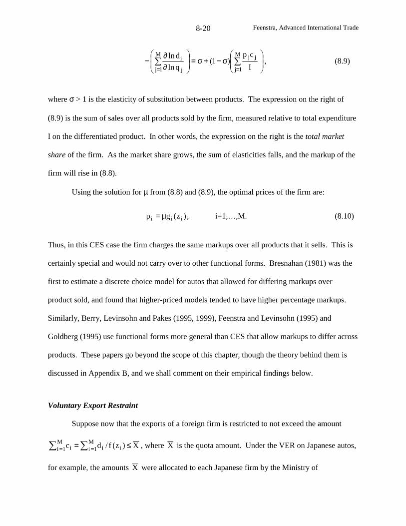
Feenstra, Advanced International Trade8-20
σ−+σ=
∂∂
− ∑∑==
M
1j
jjM
1j j
i
I
cp)1(
qln
dln, (8.9)
where σ > 1 is the elasticity of substitution between products. The expression on the right of
(8.9) is the sum of sales over all products sold by the firm, measured relative to total expenditure
I on the differentiated product. In other words, the expression on the right is the total market
share of the firm. As the market share grows, the sum of elasticities falls, and the markup of the
firm will rise in (8.8).
Using the solution for µ from (8.8) and (8.9), the optimal prices of the firm are:
,)z(gp iii µ= i=1,…,M. (8.10)
Thus, in this CES case the firm charges the same markups over all products that it sells. This is
certainly special and would not carry over to other functional forms. Bresnahan (1981) was the
first to estimate a discrete choice model for autos that allowed for differing markups over
product sold, and found that higher-priced models tended to have higher percentage markups.
Similarly, Berry, Levinsohn and Pakes (1995, 1999), Feenstra and Levinsohn (1995) and
Goldberg (1995) use functional forms more general than CES that allow markups to differ across
products. These papers go beyond the scope of this chapter, though the theory behind them is
discussed in Appendix B, and we shall comment on their empirical findings below.
Voluntary Export Restraint
Suppose now that the exports of a foreign firm is restricted to not exceed the amount
∑∑ == ≤= M1i ii
M1i i X)z(f/dc , where X is the quota amount. Under the VER on Japanese autos,
for example, the amounts X were allocated to each Japanese firm by the Ministry of
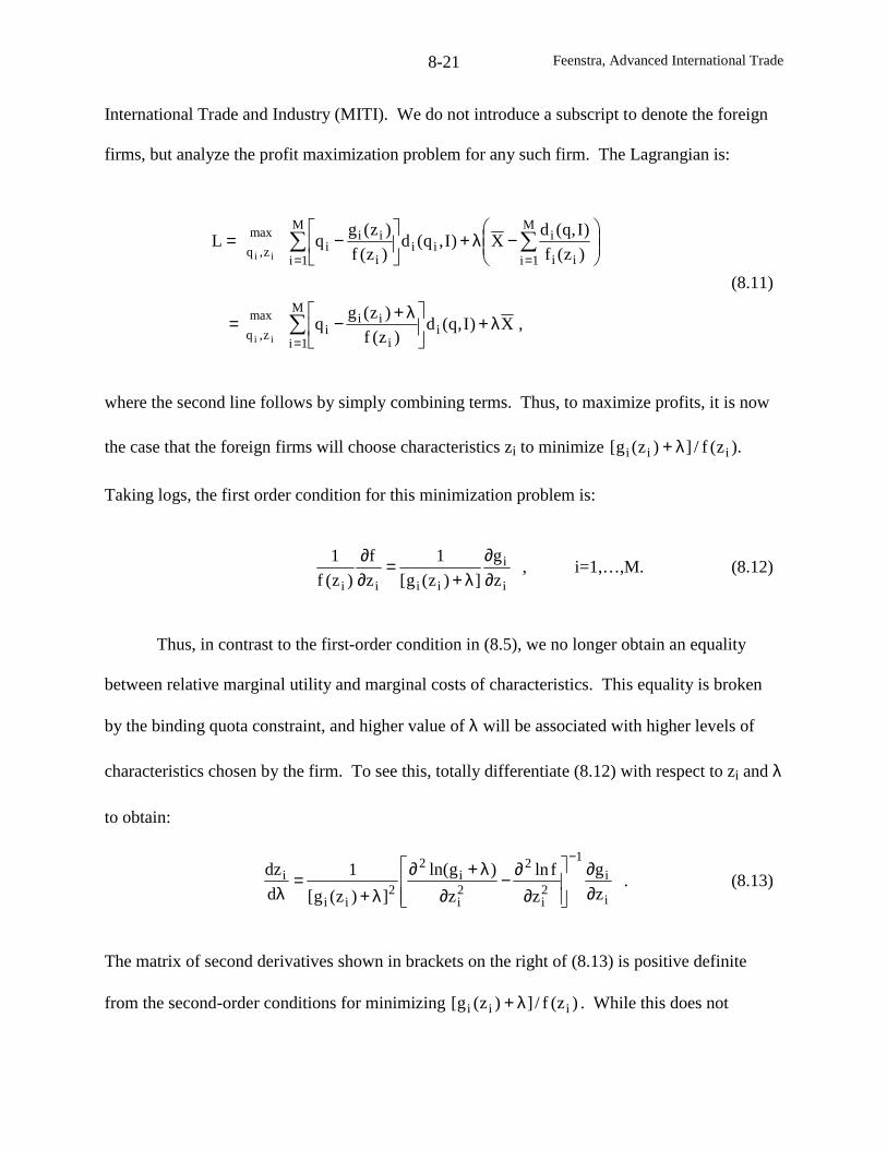
Feenstra, Advanced International Trade8-21
International Trade and Industry (MITI). We do not introduce a subscript to denote the foreign
firms, but analyze the profit maximization problem for any such firm. The Lagrangian is:
,X)I,q(d)z(f
)z(gq
)z(f
)I,q(dX)I,q(d
)z(f
)z(gqL
M
1ii
i
iiiz,q
max
M
1i ii
iM
1iii
i
iiiz,q
max
ii
ii
λ+
λ+−=
−λ+
−=
∑
∑∑
=
==
(8.11)
where the second line follows by simply combining terms. Thus, to maximize profits, it is now
the case that the foreign firms will choose characteristics zi to minimize ).z(f/])z(g[ iii λ+
Taking logs, the first order condition for this minimization problem is:
i
i
iiii z
g
])z(g[
1
z
f
)z(f
1
∂∂
λ+=
∂∂
, i=1,…,M. (8.12)
Thus, in contrast to the first-order condition in (8.5), we no longer obtain an equality
between relative marginal utility and marginal costs of characteristics. This equality is broken
by the binding quota constraint, and higher value of λ will be associated with higher levels of
characteristics chosen by the firm. To see this, totally differentiate (8.12) with respect to zi and λ
to obtain:
i
i
1
2i
2
2i
i2
2ii
i
z
g
z
fln
z
)gln(
])z(g[
1
d
dz
∂∂
∂∂−
∂λ+∂
λ+=
λ
−
. (8.13)
The matrix of second derivatives shown in brackets on the right of (8.13) is positive definite
from the second-order conditions for minimizing )z(f/])z(g[ iii λ+ . While this does not
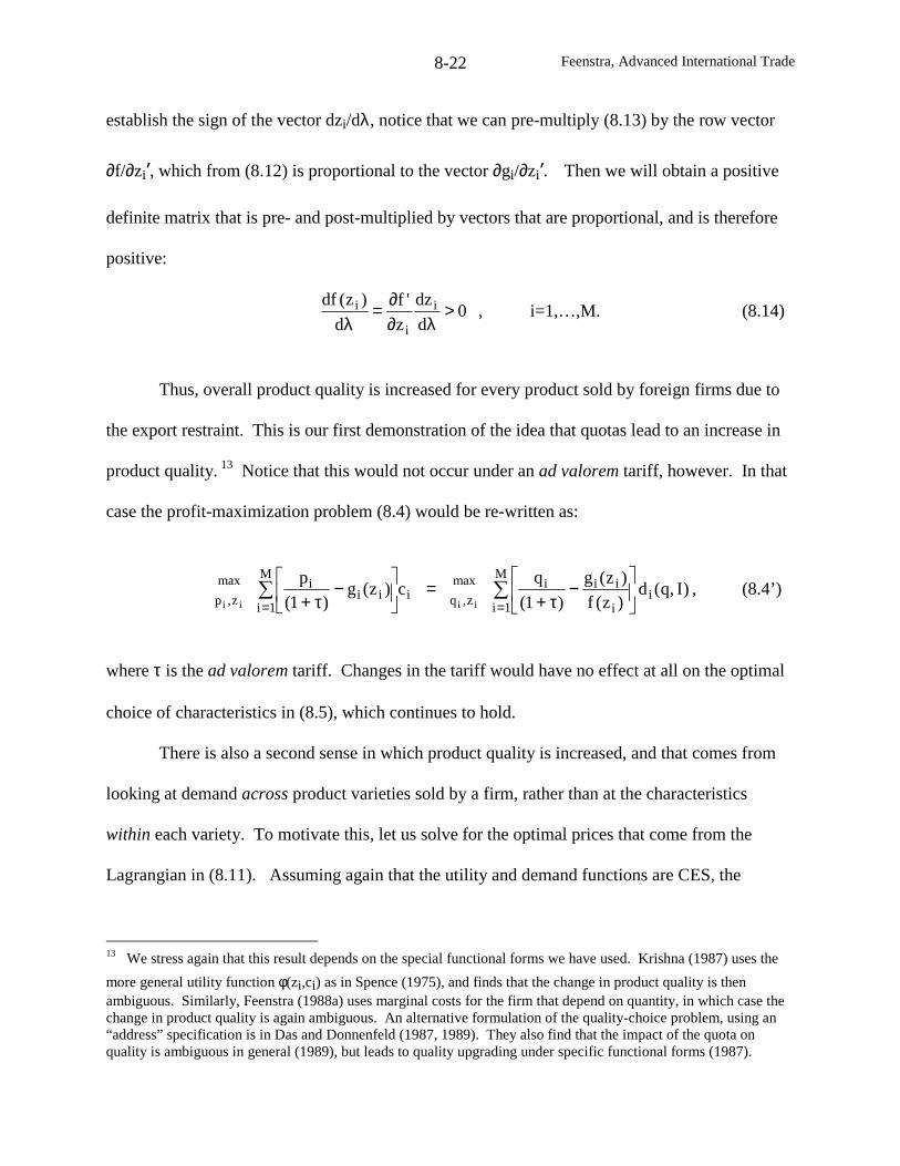
Feenstra, Advanced International Trade8-22
establish the sign of the vector dzi/dλ, notice that we can pre-multiply (8.13) by the row vector
∂f/∂zi’, which from (8.12) is proportional to the vector ∂gi/∂zi’. Then we will obtain a positive
definite matrix that is pre- and post-multiplied by vectors that are proportional, and is therefore
positive:
0d
dz
z
'f
d
)z(df i
i
i >λ∂
∂=λ
, i=1,…,M. (8.14)
Thus, overall product quality is increased for every product sold by foreign firms due to
the export restraint. This is our first demonstration of the idea that quotas lead to an increase in
product quality. 13 Notice that this would not occur under an ad valorem tariff, however. In that
case the profit-maximization problem (8.4) would be re-written as:
∑∑==
−
τ+=
−τ+
M
1ii
i
iiiz,q
maxM
1iiii
iz,p
max )I,q(d)z(f
)z(g
)1(
qc)z(g
)1(
p
iiii, (8.4’)
where τ is the ad valorem tariff. Changes in the tariff would have no effect at all on the optimal
choice of characteristics in (8.5), which continues to hold.
There is also a second sense in which product quality is increased, and that comes from
looking at demand across product varieties sold by a firm, rather than at the characteristics
within each variety. To motivate this, let us solve for the optimal prices that come from the
Lagrangian in (8.11). Assuming again that the utility and demand functions are CES, the
13 We stress again that this result depends on the special functional forms we have used. Krishna (1987) uses the
more general utility function φ(zi,ci) as in Spence (1975), and finds that the change in product quality is thenambiguous. Similarly, Feenstra (1988a) uses marginal costs for the firm that depend on quantity, in which case thechange in product quality is again ambiguous. An alternative formulation of the quality-choice problem, using an“address” specification is in Das and Donnenfeld (1987, 1989). They also find that the impact of the quota onquality is ambiguous in general (1989), but leads to quality upgrading under specific functional forms (1987).
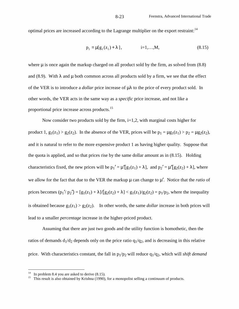
Feenstra, Advanced International Trade8-23
optimal prices are increased according to the Lagrange multiplier on the export restraint:14
])z(g[p iii λ+µ= , i=1,…,M, (8.15)
where µ is once again the markup charged on all product sold by the firm, as solved from (8.8)
and (8.9). With λ and µ both common across all products sold by a firm, we see that the effect
of the VER is to introduce a dollar price increase of µλ to the price of every product sold. In
other words, the VER acts in the same way as a specific price increase, and not like a
proportional price increase across products.15
Now consider two products sold by the firm, i=1,2, with marginal costs higher for
product 1, g1(z1) > g2(z2). In the absence of the VER, prices will be p1 = µg1(z1) > p2 = µg2(z2),
and it is natural to refer to the more expensive product 1 as having higher quality. Suppose that
the quota is applied, and so that prices rise by the same dollar amount as in (8.15). Holding
characteristics fixed, the new prices will be p1’ = µ’[g1(z1) + λ], and p2’ = µ’[g2(z2) + λ], where
we allow for the fact that due to the VER the markup µ can change to µ’. Notice that the ratio of
prices becomes (p1’/ p2’) = [g1(z1) + λ]/[g2(z2) + λ] < g1(z1)/g2(z2) = p1/p2, where the inequality
is obtained because g1(z1) > g2(z2). In other words, the same dollar increase in both prices will
lead to a smaller percentage increase in the higher-priced product.
Assuming that there are just two goods and the utility function is homothetic, then the
ratios of demands d1/d2 depends only on the price ratio q1/q2, and is decreasing in this relative
price. With characteristics constant, the fall in p1/p2 will reduce q1/q2, which will shift demand
14 In problem 8.4 you are asked to derive (8.15).15 This result is also obtained by Krishna (1990), for a monopolist selling a continuum of products.
Feenstra, Advanced International Trade8-24
towards the higher-priced product so that d1/d2 increases. This shift towards the higher-quality
product corresponds to an increase in average quality. Furthermore, notice that the change in
average quality would not occur with an ad valorem tariff, since that would have no impact on
the relative price.
The above description of quality upgrading due to shifts in demand is called the
“Washington apples” effect, after the example given by Alchian and Allen (1964, pp. 74-75).
They noted that while the state of Washington grows apples of many varieties, it appeared that
the best apples were shipped the furthest distance, to east coast markets. This is explained by
treating the transport costs as the same for each apple. Transport therefore acts like a specific
price increase, which lowers the relative price of the higher-quality apples in more distance
markets. Accordingly, we expect to see the best apples shipped to the east coast, which raises
the average quality in those markets.
In summary, there are two reasons to expect import quality to rise with a quota on the
number of units sold: due to the increase in characteristics chosen by the exporting firms; and
due to the shift in demand towards the higher-quality products. These two effects can certainly
work together. In the model above, the demands di(qi, I) for quality-adjusted consumption
f(zi)ci, are determined by the quality-adjusted prices qi ≡ pi/f(zi). So let us see how these prices
are affected by the quota, even as characteristics change.
Using (8.15), the quality-adjusted prices are written as qi = µ[gi(zi)+λ]/fi(zi). From our
discussion following (8.8), we know that [gi(zi)+λ]/fi(zi) is minimized over the choice of
characteristics zi. Then by the envelope theorem, when differentiating this expression we can
Feenstra, Advanced International Trade8-25
treat the characteristics as fixed. Accordingly, we can compute the change in quality-adjusted
prices due to the quota as:
iii
i
pd
lnd
])z(g[
1
d
lnd
d
qlnd µ+λµ=
λ++
λµ=
λ. (8.16)
The first term on the right of (8.16) is the change in markup due to the VER, which is common
across products, while the second term is smallest for the highest-priced products. Therefore, we
will observe the smallest relative increase in quality-adjusted price for those products with the
highest prices. This can be expected to shift demand towards the highest-priced products, just as
in the “Washington apples” effect.
Measuring Quality-Upgrading due to Quotas
We turn now to an application of the above theory to “voluntary export restraint” (VER)
imposed on Japanese autos by the United State. Recall that with unemployment in the
automobile industry growing in the 1979-80 and profits falling, Ford Motor Company and the
UAW applied to the U.S. ITC for section 201 protection. This application was denied on the
grounds that the U.S. recession appeared to be a greater cause of unemployment and falling
profits than were rising imports from Japan.
Faced with this negative outcome, several congressmen from mid-western states pursued
protection for automobiles via other means. Senators Danforth and Bentsen introduced a bill to
restrict imports, which would have restricted Japanese automobiles imports into the U.S. to 1.6
million units during 1981, 1982 and 1983. Indeed, this bill was scheduled for revision in the
Senate Finance Committee on May 12, 1981. Clearly aware of this pending legislation, the
Japanese government announced on May 1 that it would “voluntarily” limit the sales of
Feenstra, Advanced International Trade8-26
automobiles in the U.S. market. For the period April 1981 – March 1982, this limit was set at
1.83 million autos, including 1.68 million cars exported to the U.S., 82,500 utility vehicles, and
70,000 vehicles exported to Puerto Rico. This limit was in place until March 1984, after which it
was raised to 2.02 and then 2.51 million vehicles annually until March 1992, as shown in Table
8.2 where we compare the actual imports with the VER limits. It is evident that the VER was
nearly exactly satisfied in early years, and remained binding until 1987. After that, however,
actual imports were below the VER so that by March 1994 it was discontinued. The reason that
imports fell below the VER after 1987 was because Japanese companies had begun assembling
cars in the United States, so imports naturally fell.
Our interest, then, is in the effects of the VER during the early years. To estimate the
change in product quality, initially consider the case where there is no VER. Assuming that
marginal costs take the form ln gi(zit) = β’zit + ξit, where ξit is a random error that reflects
unmeasured characteristics, and we add the subscript t to denote years. Then the first order
condition (8.10) is written in logs as:
itittit z'pln ξ+β+α= , i=1,…,M, (8.17)
where αt = ln µt reflects the markups. We should also be indexing αt by firms (since the
markups differ across firms), but will omit this notation. Equation (8.17) is a log-linear
regression of prices on characteristics and is called a “hedonic regression.” Our derivation
shows that this is a valid representation of the equilibrium under imperfect competition provided
that markups are the same across products (as in the CES case). Furthermore, using the equality
between relative marginal utility from each characteristic, on the left of (8.5), and relative
marginal cost on the right, we can interpret the coefficients β in (8.17) in either way.
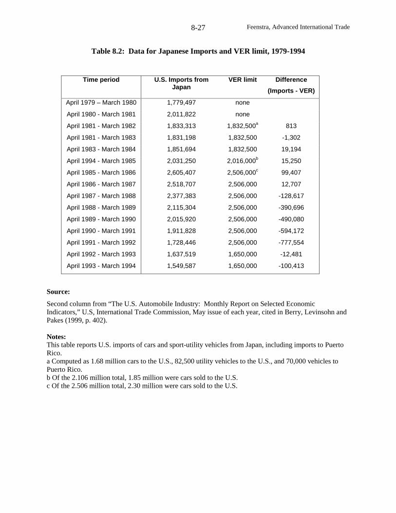
Feenstra, Advanced International Trade8-27
Table 8.2: Data for Japanese Imports and VER limit, 1979-1994
Time period U.S. Imports fromJapan
VER limit Difference
(Imports - VER)
April 1979 – March 1980 1,779,497 none
April 1980 - March 1981 2,011,822 none
April 1981 - March 1982 1,833,313 1,832,500a 813
April 1981 - March 1983 1,831,198 1,832,500 -1,302
April 1983 - March 1984 1,851,694 1,832,500 19,194
April 1994 - March 1985 2,031,250 2,016,000b 15,250
April 1985 - March 1986 2,605,407 2,506,000c 99,407
April 1986 - March 1987 2,518,707 2,506,000 12,707
April 1987 - March 1988 2,377,383 2,506,000 -128,617
April 1988 - March 1989 2,115,304 2,506,000 -390,696
April 1989 - March 1990 2,015,920 2,506,000 -490,080
April 1990 - March 1991 1,911,828 2,506,000 -594,172
April 1991 - March 1992 1,728,446 2,506,000 -777,554
April 1992 - March 1993 1,637,519 1,650,000 -12,481
April 1993 - March 1994 1,549,587 1,650,000 -100,413
Source:
Second column from “The U.S. Automobile Industry: Monthly Report on Selected EconomicIndicators,” U.S, International Trade Commission, May issue of each year, cited in Berry, Levinsohn andPakes (1999, p. 402).
Notes:This table reports U.S. imports of cars and sport-utility vehicles from Japan, including imports to PuertoRico.a Computed as 1.68 million cars to the U.S., 82,500 utility vehicles to the U.S., and 70,000 vehicles toPuerto Rico.b Of the 2.106 million total, 1.85 million were cars sold to the U.S.c Of the 2.506 million total, 2.30 million were cars sold to the U.S.
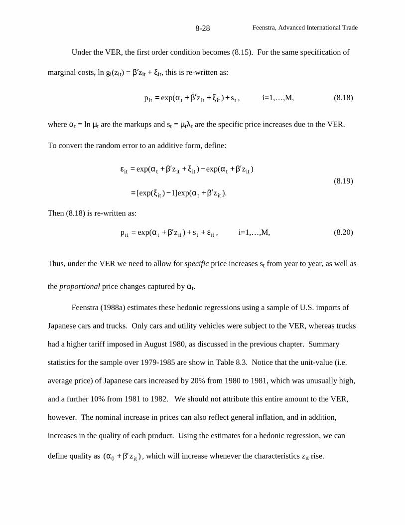
Feenstra, Advanced International Trade8-28
Under the VER, the first order condition becomes (8.15). For the same specification of
marginal costs, ln gi(zit) = β’zit + ξit, this is re-written as:
titittit s)zexp(p +ξ+β′+α= , i=1,…,M, (8.18)
where αt = ln µt are the markups and st = µtλt are the specific price increases due to the VER.
To convert the random error to an additive form, define:
).zexp(]1)[exp(
)zexp()zexp(
ittit
ittitittit
β′+α−ξ=
β′+α−ξ+β′+α=ε(8.19)
Then (8.18) is re-written as:
ittittit s)zexp(p ε++β′+α= , i=1,…,M, (8.20)
Thus, under the VER we need to allow for specific price increases st from year to year, as well as
the proportional price changes captured by αt.
Feenstra (1988a) estimates these hedonic regressions using a sample of U.S. imports of
Japanese cars and trucks. Only cars and utility vehicles were subject to the VER, whereas trucks
had a higher tariff imposed in August 1980, as discussed in the previous chapter. Summary
statistics for the sample over 1979-1985 are show in Table 8.3. Notice that the unit-value (i.e.
average price) of Japanese cars increased by 20% from 1980 to 1981, which was unusually high,
and a further 10% from 1981 to 1982. We should not attribute this entire amount to the VER,
however. The nominal increase in prices can also reflect general inflation, and in addition,
increases in the quality of each product. Using the estimates for a hedonic regression, we can
define quality as )z'( it0 β+α , which will increase whenever the characteristics zit rise.
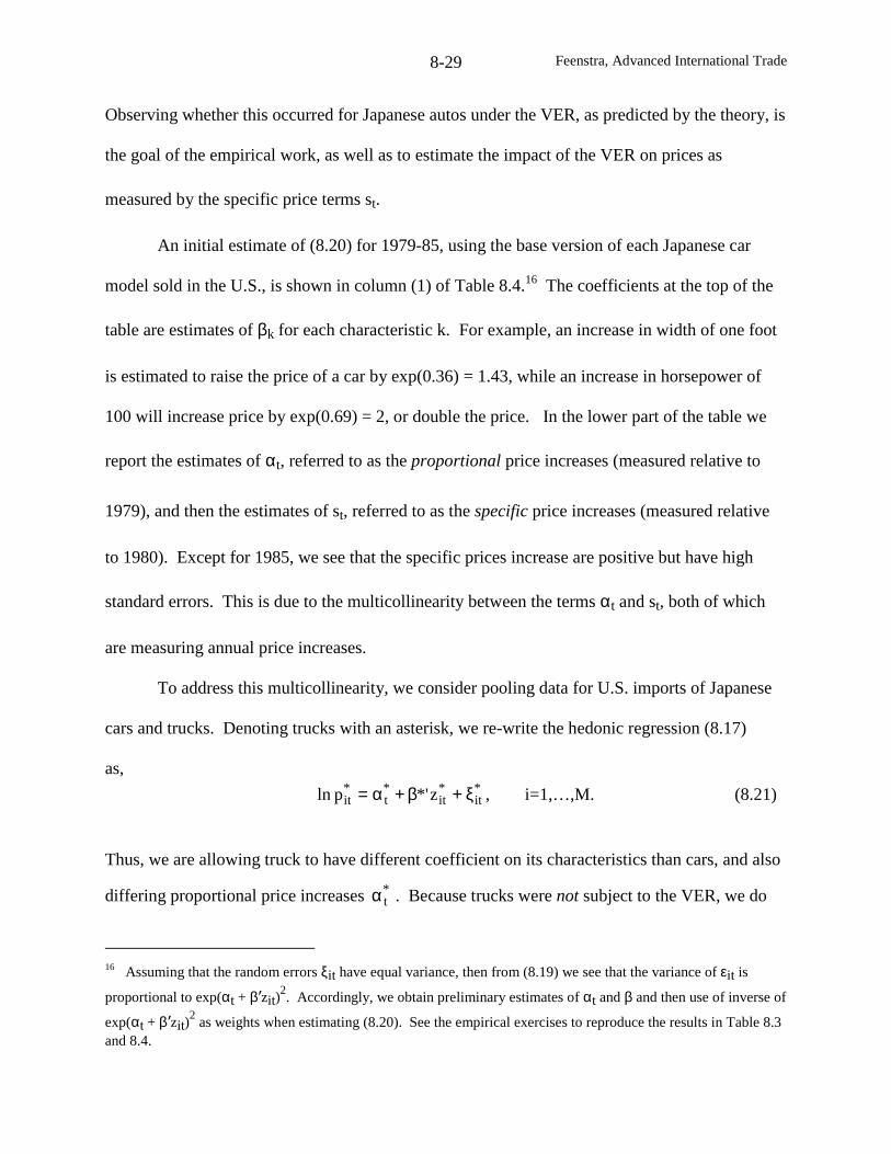
Feenstra, Advanced International Trade8-29
Observing whether this occurred for Japanese autos under the VER, as predicted by the theory, is
the goal of the empirical work, as well as to estimate the impact of the VER on prices as
measured by the specific price terms st.
An initial estimate of (8.20) for 1979-85, using the base version of each Japanese car
model sold in the U.S., is shown in column (1) of Table 8.4.16 The coefficients at the top of the
table are estimates of βk for each characteristic k. For example, an increase in width of one foot
is estimated to raise the price of a car by exp(0.36) = 1.43, while an increase in horsepower of
100 will increase price by exp(0.69) = 2, or double the price. In the lower part of the table we
report the estimates of αt, referred to as the proportional price increases (measured relative to
1979), and then the estimates of st, referred to as the specific price increases (measured relative
to 1980). Except for 1985, we see that the specific prices increase are positive but have high
standard errors. This is due to the multicollinearity between the terms αt and st, both of which
are measuring annual price increases.
To address this multicollinearity, we consider pooling data for U.S. imports of Japanese
cars and trucks. Denoting trucks with an asterisk, we re-write the hedonic regression (8.17)
as,*it
*it
*t
*it z*'pln ξ+β+α= , i=1,…,M. (8.21)
Thus, we are allowing truck to have different coefficient on its characteristics than cars, and also
differing proportional price increases *tα . Because trucks were not subject to the VER, we do
16 Assuming that the random errors ξit have equal variance, then from (8.19) we see that the variance of εit is
proportional to exp(αt + β’zit)2. Accordingly, we obtain preliminary estimates of αt and β and then use of inverse of
exp(αt + β’zit)2 as weights when estimating (8.20). See the empirical exercises to reproduce the results in Table 8.3
and 8.4.
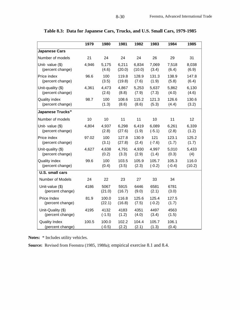
Feenstra, Advanced International Trade8-30
Table 8.3: Data for Japanese Cars, Trucks, and U.S. Small Cars, 1979-1985
1979 1980 1981 1982 1983 1984 1985
Japanese Cars
Number of models 21 24 24 24 26 29 31
Unit- value ($) 4,946 5,175 6,211 6,834 7,069 7,518 8,038(percent change) (4.6) (20.0) (10.0) (3.4) (6.4) (6.9)
Price index 96.6 100 119.8 128.9 131.3 138.9 147.8(percent change) (3.5) (19.8) (7.6) (1.9) (5.8) (6.4)
Unit-quality ($) 4,361 4,473 4,867 5,253 5,637 5,862 6,130(percent change) (2.6) (8.8) (7.9) (7.3) (4.0) (4.6)
Quality index 98.7 100 108.6 115.2 121.3 126.6 130.6(percent change) (1.3) (8.6) (8.6) (5.3) (4.4) (3.2)
Japanese Trucks*
Number of models 10 10 11 11 10 11 12
Unit- value ($) 4,804 4,937 6,298 6,419 6,089 6,261 6,339(percent change) (2.8) (27.6) (1.9) (-5.1) (2.8) (1.2)
Price index 97.02 100 127.8 130.9 121 123.1 125.2(percent change) (3.1) (27.8) (2.4) (-7.6) (1.7) (1.7)
Unit-quality ($) 4,627 4,638 4,791 4,930 4,997 5,010 5,433(percent change) (0.2) (3.3) (2.9) (1.4) (0.3) (4)
Quality index 99.6 100 103.5 105.9 105.7 105.3 116.0(percent change) (0.4) (3.5) (2.3) (-0.2) (-0.4) (10.2)
U.S. small cars
Number of Models 24 22 23 27 33 34
Unit-value ($) 4186 5067 5915 6446 6581 6781(percent change) (21.0) (16.7) (9.0) (2.1) (3.0)
Price Index 81.9 100.0 116.8 125.6 125.4 127.5(percent change) (22.1) (16.8) (7.5) (-0.2) (1.7)
Unit-Quality ($) 4195 4132 4183 4351 4497 4563(percent change) (-1.5) (1.2) (4.0) (3.4) (1.5)
Quality Index 100.5 100.0 102.2 104.4 105.7 106.1(percent change) (-0.5) (2.2) (2.1) (1.3) (0.4)
Notes: * Includes utility vehicles.
Source: Revised from Feenstra (1985, 1988a); empirical exercise 8.1 and 8.4.
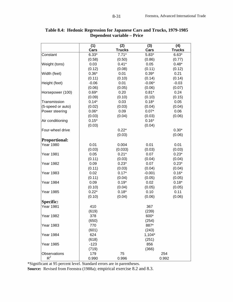
Feenstra, Advanced International Trade8-31
Table 8.4: Hedonic Regression for Japanese Cars and Trucks, 1979-1985Dependent variable – Price
(1)Cars
(2)Trucks
(3)Cars
(4)Trucks
Constant 6.33* 7.71* 5.83* 6.63*(0.58) (0.50) (0.86) (0.77)
Weight (tons) 0.03 0.41* 0.05 0.48*(0.12) (0.08) (0.11) (0.12)
Width (feet) 0.36* 0.01 0.39* 0.21(0.11) (0.10) (0.14) (0.14)
Height (feet) -0.06 0.01 -0.06* -0.03(0.06) (0.05) (0.06) (0.07)
Horsepower (100) 0.69* 0.20 0.81* 0.24(0.09) (0.10) (0.10) (0.15)
Transmission 0.14* 0.03 0.18* 0.05(5-speed or auto) (0.02) (0.03) (0.04) (0.04)Power steering 0.06* 0.09 0.07* 0.06
(0.03) (0.04) (0.03) (0.06)Air conditioning 0.15* 0.16*
(0.03) (0.04)Four-wheel drive 0.22* 0.30*
(0.03) (0.06)Proportional:Year 1980 0.01 0.004 0.01 0.01
(0.03) (0.033) (0.03) (0.03)Year 1981 0.05 0.21* 0.07 0.23*
(0.11) (0.03) (0.04) (0.04)Year 1982 0.09 0.23* 0.07 0.23*
(0.11) (0.03) (0.04) (0.04)Year 1983 0.02 0.17* -0.001 0.16*
(0.11) (0.04) (0.05) (0.05)Year 1984 0.09 0.19* 0.02 0.18*
(0.10) (0.04) (0.05) (0.05)Year 1985 0.22* 0.18* 0.10 0.11
(0.10) (0.04) (0.06) (0.06)Specific:Year 1981 410 367
(619) (239)Year 1982 378 600*
(650) (254)Year 1983 770 887*
(601) (243)Year 1984 624 1,104*
(618) (251)Year 1985 -123 856
(719) (366)Observations 179 75 254
R2 0.990 0.996 0.992*Significant at 95 percent level. Standard errors are in parentheses.Source: Revised from Feenstra (1988a); empirical exercise 8.2 and 8.3.
Feenstra, Advanced International Trade8-32
not include any specific price increases in this regression. Estimates of (8.21) using the data on
trucks are shown in regression (2) of Table 8.4.17
We now consider testing the hypothesis that the year-to-year price changes in Japanese
cars and truck exports to the U.S. would be the same, after correcting for the trade policies in
each product. Cars were subject to the VER after April 1981, whereas trucks imported from
Japan were subject to an increase in the tariff from 4% to 25% after August 1980, as discussed in
the previous chapter. Feenstra (1988a) argues that the 21% increase in the wholesale price of
trucks as they cross the border would be reflected by at most a 16% increase in the retail price.18
Accordingly, we consider testing the hypothesis that the proportional year increase for trucks,
*tα , is 0.16 greater than the proportional year increase for cars, αt, for 1981 and later years:
16.0t*t +α=α for t=1981,82,…,85. (8.22)
Feenstra (1988a) finds that this hypothesis is accepted in all years except 1985, and so it is
imposed on the subsequent estimation except for that year.
In columns (3) and (4) of Table 8.4, we re-estimate the regressions for cars and trucks,
while imposing the cross-equation restraint (8.22) for t=1981,…,84. Notice that this reduces
the standard errors on the specific price increases for cars substantially. By 1984-85, the impact
of the VER is to increase the price of cars by about $1,000 on average. This is an estimate of the
pure price increase due to the quota, after correcting for changes in the characteristics of
Japanese cars. Multiplying this by the average 1984-85 imports of some 2.2 million, we obtain
17 Utility vehicles are given the same hedonic coefficients β* as trucks, but use the year coefficients st and αt ofcars, since utility vehicles were subject to the VER.18 This can be thought of as a pass-through of 0.75 from the 21% increase in tariff to a 16% increase in retail price.This is somewhat higher than the pass-through of 0.58 for the truck tariff estimated in Feenstra (1989), anddiscussed in the previous chapter.
Feenstra, Advanced International Trade8-33
an estimate of the quota rents of $2.2 billion annually in 1984-85.
This estimate equals lower end of the quota rents for autos shown in Table 8.1. Where do
the higher estimates come from? It turns out that along with the increase in Japanese car prices,
European producers selling in the U.S. also raised their prices substantially – by nearly one-third,
as estimated by Dinopoulos and Kreinin (1988). They calculate a U.S. welfare loss due to this
increase in European prices of some $3.4 billion in 1984, which exceeds the loss due to quota
rents transferred to Japan. This nicely illustrates the result argued by Harris (1985) and Krishna
(1989), that a VER will act as a “facilitating practice” and leads to more collusive behavior in the
market where it is imposed. For American small cars we also show a substantial increase in
prices at the bottom of Table 8.3: by 21% from 1979-80 and 17% from 1980-81. Some of this
increase occurred before the VER, but it appears that this quota allowed American producers to
maintain and continue large prices increases.
What about the change in product quality for Japanese imports? In fact, there was a
considerable upgrading of model characteristics at just the time that the VER was imposed. In
Table 8.3, we show the “unit-quality,” which is computed as )z'( it0 β+α and then averaged
across all models. This increases by 8.8% from 1980 to 1981, and another 7.9% over 1981-82
and 7.3% over 1982-83. The dollar increase in quality over 1980-85 is $1,650, which reflects
higher values of the characteristics applied to each model. This vastly exceeds the quality
change for trucks or U.S. small cars as shown in Table 8.3. These observations strongly support
the theoretical prediction that Japanese producers raised characteristics to increase the quality of
cars due to the VER, but this did not occur under the ad valorem tariff in trucks.
Aside from characteristics, recall that there is a second way that average quality can
increase following the VER, and that is from shifting demand towards the highest-quality
Feenstra, Advanced International Trade8-34
products because their effective prices have the lowest percentage increase in prices. Evidence
supporting this “Washington apples” effect can also be seen from Table 8.3. In addition to the
unit-value and unit-quality, we show there a price and quality index. The difference between the
unit-value and price index is that the former uses the quantity sold of each car in that year as a
weight in forming the average, whereas the price index uses fixed weights from year to year
when forming the index.19 In other words, a shift in demand towards more-expensive models
will increase the unit-value, but will have no effect on the price index. It follows that the ratio of
the unit-value to the price index can be used as a measure of “product mix,” i.e. an increase in
the unit-value exceeding the price index indicates that demand has shifted towards more-
expensive models.
Returning to Table 8.3, we see that the unit-value indeed increased by more than the price
index: the cumulative rise in the unit-value is (8,038 – 5,175)/5,175 = 55.3% over 1980-85,
whereas the price index increased by 47.8%. Similarly, the cumulative rise in the unit-quality is
(8.5,862 – 4,473)/4,473 = 37% over 1980-85, whereas the quality index increased by 30.6%. By
either measure, there is a noticeable shift in demand towards the higher-priced and higher-quality
cars, as predicted by the “Washington apples” effect. In addition, the change in the quality-
adjusted prices (measured by )z'pln itit β∆−∆ are graphed in Figure 8.5, for 1980-1985. It can
be seen that many of the highest priced models had below-average increases in the their quality-
adjusted price, as predicted by (8.16).
We note that the non-uniform change in prices illustrated in Figure 8.5 can be expected to
have a deadweight loss (as compared to a uniform percentage change in prices). A formula for
19 The price and quality indexes shown in Table 8.3 are constructed as the Fisher Ideal index. The formula for thisindex is discussed in Appendix A, and you are asked to calculate this index in empirical exercise 8.1 and 8.4.
Feenstra, Advanced International Trade8-35
measured the deadweight is developed in Boorstein and Feenstra (1991), who studied quality
upgrading due to the “Washington applies” effect for the quota on U.S. steel imports during
1969-74.20 That formula was extended to incorporate rising characteristics due to the autos VER
by Feenstra (1993), who finds that the deadweight loss is high: between one-quarter and one-
third of the value of quality upgrading in each year, or about $500 by 1985. This loss is in
addition to the foregone rents of about $1,000 per imported Japanese car in 1984-85, which
indicates that the deadweight loss of quality change adds a substantial component to the welfare
cost of the VER.21
Our estimate of the quota rents over 1980-85 can be compared to other studies. Ries
(1993) studies the change in stock prices of Japanese auto producers and parts suppliers during
the weeks in 1981 when this policy was being formulated. He finds strong evidence of positive
returns to the stocks of Japanese auto producers during this period, though only after it became
clear that MITI would administer the quotas to each producer (so that they would capture the
rents). In contrast, only the largest parts suppliers obtain abnormal stock during this period.
Further supportive evidence is obtained by Goldberg (1995), who finds that the VER was
binding in 1983-84 and 1986-87, with the highest rents in the earlier years.
The only study to question this conclusion is Berry, Levinsohn and Pakes (1999)
(hereafter BLP), who argue that the VER was not binding in the early years, and became binding
in 1986. They obtain the highest estimates for the price effect of the quota (like st in our
notation) in the years 1987-90. This is a puzzling finding, since from Table 8.2 we know that
Japanese imports fell short of the VER limit during March 1987 – April 1988 and in later years.
20 Goolsbee (2001) applies this formula to measure the deadweight loss due to non-uniform capital taxation.21 The deadweight loss due to quality change under quotas in U.S. dairy imports is estimated by Anderson (1985,1988). Anderson and Neary (1996) develop general methods for measuring the deadweight loss of non-uniformtariff or quota structures.
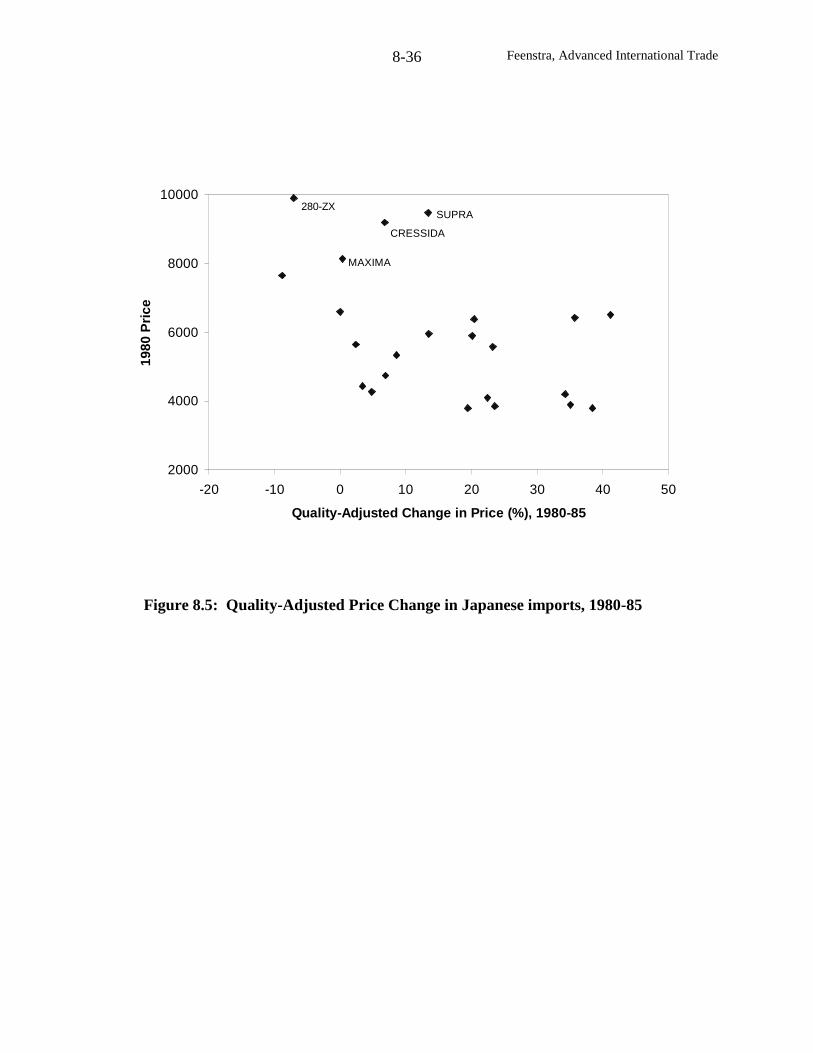
Feenstra, Advanced International Trade8-36
2000
4000
6000
8000
10000
-20 -10 0 10 20 30 40 50
Quality-Adjusted Change in Price (%), 1980-85
1980
Pri
ce
280-ZXSUPRA
CRESSIDA
MAXIMA
Figure 8.5: Quality-Adjusted Price Change in Japanese imports, 1980-85
Feenstra, Advanced International Trade8-37
For the remainder of this section, we discuss possible explanations for the differing findings of
Feenstra (1988a) and BLP.
We begin by extending our sample from 1979-1985, as used in the regressions of Table
8.4, to 1979-1990. The new estimates of the car and truck regressions (8.20) and (8.21) are
shown in Table 8.5. In column (1) and (2) we report the car and truck regressions without any
cross-equation constraints, while in columns (3) and (4) we make use the constraint in (8.22) for
t=1981,…,84.22 As before, making use of this cross-equation constraint is effective in reducing
the standard errors of the specific price increases.
Including the additional five years of data turns out to have a substantial impact on some
of the hedonic coefficients: for example, the coefficient on width in the car regression is much
higher than in Table 8.4, while the coefficient on horsepower is smaller. With this change in the
hedonic coefficients, the specific price effect of the VER in the early years is reduced somewhat:
in 1984, we estimate a price increase due to the VER of $812 in column (3) of Table 8.5, as
compared with $1,104 in column (3) of Table 8.4. This price impact in small in 1985 in both
tables, but the effect of the VER grows after that and peaks in 1987, where we estimates quota
rents of $1,164 per vehicle in column (3) of Table 8.5. So by extending the sample, we find that
the VER is still binding in 1987. After that year, however, our estimates give highly imprecise
estimates of the price impact of the VER, ranging from positive in column (1) to negative in
column (3), but in all cases insignificantly different from zero. Consistent with the fact that
Japanese exports to the United States fell short of the VER limit, we do not identify any
significant impact of this trade restriction on prices after 1987.
22 As in note 17, utility vehicles are given the same hedonic coefficients β* as trucks, but using the year
coefficients st and αt of cars, since utility vehicles were subject to the VER
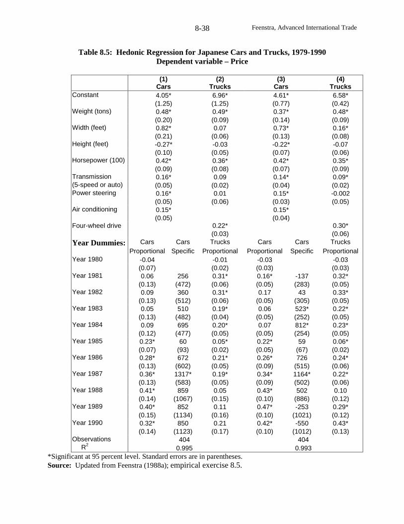
Feenstra, Advanced International Trade8-38
Table 8.5: Hedonic Regression for Japanese Cars and Trucks, 1979-1990Dependent variable – Price
(1)Cars
(2)Trucks
(3)Cars
(4)Trucks
Constant 4.05* 6.96* 4.61* 6.58*(1.25) (1.25) (0.77) (0.42)
Weight (tons) 0.48* 0.49* 0.37* 0.48*(0.20) (0.09) (0.14) (0.09)
Width (feet) 0.82* 0.07 0.73* 0.16*(0.21) (0.06) (0.13) (0.08)
Height (feet) -0.27* -0.03 -0.22* -0.07(0.10) (0.05) (0.07) (0.06)
Horsepower (100) 0.42* 0.36* 0.42* 0.35*(0.09) (0.08) (0.07) (0.09)
Transmission 0.16* 0.09 0.14* 0.09*(5-speed or auto) (0.05) (0.02) (0.04) (0.02)Power steering 0.16* 0.01 0.15* -0.002
(0.05) (0.06) (0.03) (0.05)Air conditioning 0.15* 0.15*
(0.05) (0.04)Four-wheel drive 0.22* 0.30*
(0.03) (0.06)Year Dummies: Cars Cars Trucks Cars Cars Trucks
Proportional Specific Proportional Proportional Specific ProportionalYear 1980 -0.04 -0.01 -0.03 -0.03
(0.07) (0.02) (0.03) (0.03)Year 1981 0.06 256 0.31* 0.16* -137 0.32*
(0.13) (472) (0.06) (0.05) (283) (0.05)Year 1982 0.09 360 0.31* 0.17 43 0.33*
(0.13) (512) (0.06) (0.05) (305) (0.05)Year 1983 0.05 510 0.19* 0.06 523* 0.22*
(0.13) (482) (0.04) (0.05) (252) (0.05)Year 1984 0.09 695 0.20* 0.07 812* 0.23*
(0.12) (477) (0.05) (0.05) (254) (0.05)Year 1985 0.23* 60 0.05* 0.22* 59 0.06*
(0.07) (93) (0.02) (0.05) (67) (0.02)Year 1986 0.28* 672 0.21* 0.26* 726 0.24*
(0.13) (602) (0.05) (0.09) (515) (0.06)Year 1987 0.36* 1317* 0.19* 0.34* 1164* 0.22*
(0.13) (583) (0.05) (0.09) (502) (0.06)Year 1988 0.41* 859 0.05 0.43* 502 0.10
(0.14) (1067) (0.15) (0.10) (886) (0.12)Year 1989 0.40* 852 0.11 0.47* -253 0.29*
(0.15) (1134) (0.16) (0.10) (1021) (0.12)Year 1990 0.32* 850 0.21 0.42* -550 0.43*
(0.14) (1123) (0.17) (0.10) (1012) (0.13)Observations 404 404
R20.995 0.993
*Significant at 95 percent level. Standard errors are in parentheses.Source: Updated from Feenstra (1988a); empirical exercise 8.5.
Feenstra, Advanced International Trade8-39
In contrast, BLP continue to find a significant price impact of the VER through 1990, but
no significant effect before 1986. I believe that the reason for this has to do with the way that
BLP model the supply side of the market. They model marginal costs for Japanese producers as
determined by time trends and wages, with the exchange rate entering insignificantly. This
formulation predicts that a steady increase in prices would have occurred over 1980-85 even
without the VER, so the VER does not appear to be binding in their estimates. But this predicted
increase in prices is contradicted by the actual movement in truck prices, which rose due to the
tariff in 1980-81 but were quite stable or fell in some years after this (see Table 8.3). The free
trade change in car prices that we have used are the same as for trucks, but correcting for the
tariff as in (8.22). Therefore, we are using a lower increase in free trade car prices than BLP,
which accounts for difference in our findings through 1985.
Like BLP, we find that the VER is binding in 1986 and 1987, but after this time we begin
to estimate a rather large proportional increase in car prices, so the specific price effect of the
VER becomes smaller and insignificant. In contrast, the free trade increase in prices allowed by
BLP is still dominated by the time trends and wages entering marginal costs, and it turns out that
these are not enough to explain the actual increase in Japanese prices: hence, they estimate that
the VER is binding after 1987, even though actual exports fell short of the VER limit.
Export Subsidies
We turn now to our second major topic for the chapter, which is the application of export
subsidies. These are used by developing and industrial countries alike to support their industries.
There is little doubt that these subsidies are welcomed by the firms receiving them, and this
might explain their use in a political economy model, as we examine in the next chapter. But in
this chapter we are concerned with social welfare, which means that the revenue cost of the
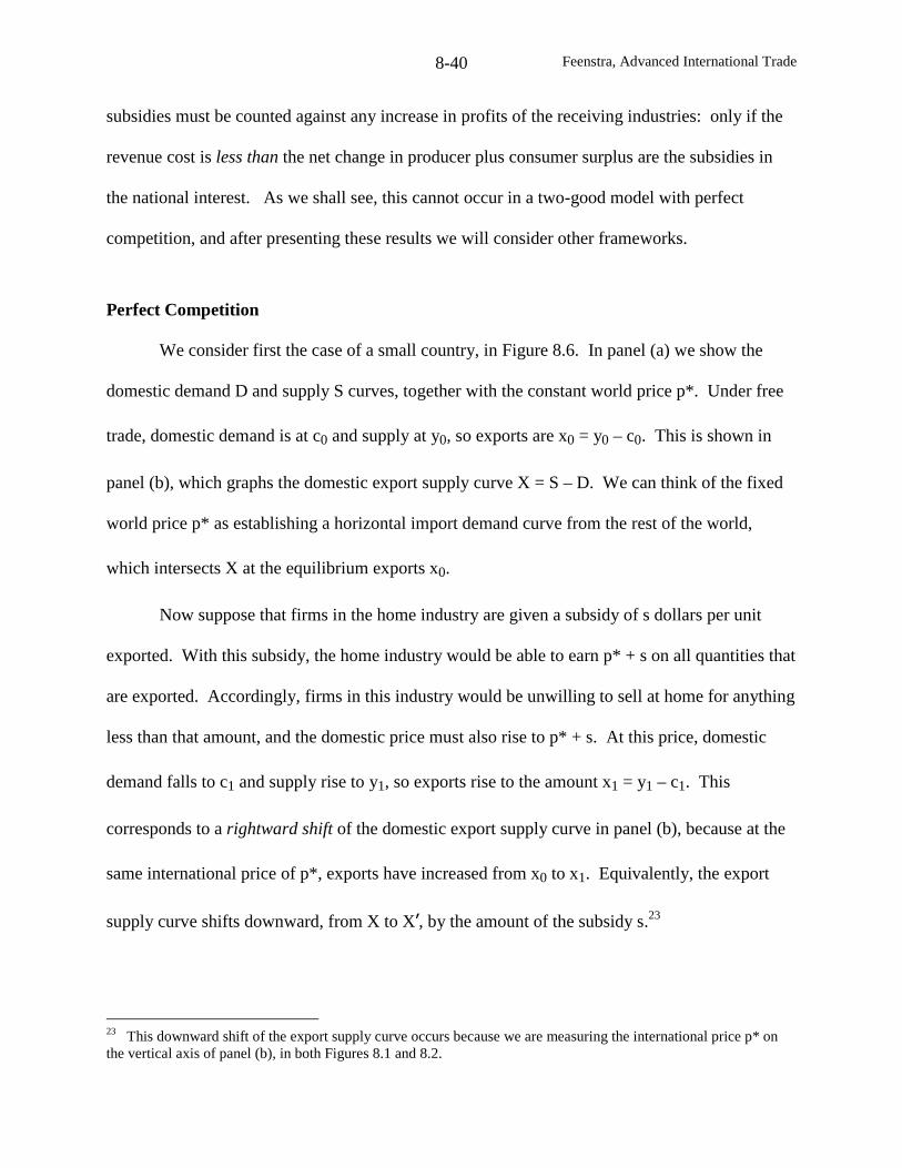
Feenstra, Advanced International Trade8-40
subsidies must be counted against any increase in profits of the receiving industries: only if the
revenue cost is less than the net change in producer plus consumer surplus are the subsidies in
the national interest. As we shall see, this cannot occur in a two-good model with perfect
competition, and after presenting these results we will consider other frameworks.
Perfect Competition
We consider first the case of a small country, in Figure 8.6. In panel (a) we show the
domestic demand D and supply S curves, together with the constant world price p*. Under free
trade, domestic demand is at c0 and supply at y0, so exports are x0 = y0 – c0. This is shown in
panel (b), which graphs the domestic export supply curve X = S – D. We can think of the fixed
world price p* as establishing a horizontal import demand curve from the rest of the world,
which intersects X at the equilibrium exports x0.
Now suppose that firms in the home industry are given a subsidy of s dollars per unit
exported. With this subsidy, the home industry would be able to earn p* + s on all quantities that
are exported. Accordingly, firms in this industry would be unwilling to sell at home for anything
less than that amount, and the domestic price must also rise to p* + s. At this price, domestic
demand falls to c1 and supply rise to y1, so exports rise to the amount x1 = y1 – c1. This
corresponds to a rightward shift of the domestic export supply curve in panel (b), because at the
same international price of p*, exports have increased from x0 to x1. Equivalently, the export
supply curve shifts downward, from X to X’, by the amount of the subsidy s.23
23 This downward shift of the export supply curve occurs because we are measuring the international price p* onthe vertical axis of panel (b), in both Figures 8.1 and 8.2.
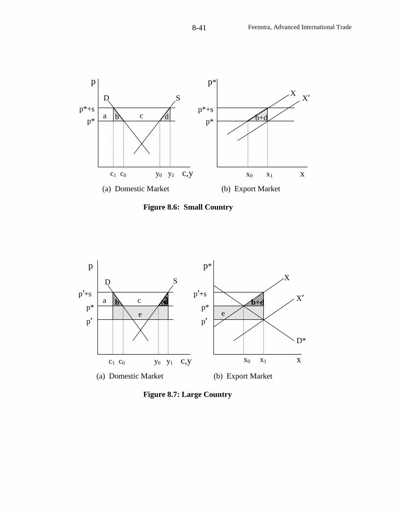
Feenstra, Advanced International Trade8-41
a c b+db
p*
p*+s
p*
p
p*+s
p*
c1 c0 y0 y1 c,y x0 x1 x
D SX
X’
(a) Domestic Market (b) Export Market
Figure 8.6: Small Country
x0 x1c1 c0 y0 y1 c,y
XD
a c
p
p’+s
p*
p’
D*
x
X’
(a) Domestic Market (b) Export Market
Figure 8.7: Large Country
p*
p’+s
p*
p’
d
S
b d
e
b+de
Feenstra, Advanced International Trade8-42
The welfare effect of the subsidy can be ready calculated in panel (a) as: –(a+b)
consumer surplus loss + (a+b+c) producer surplus gain – (b+c+d) subsidy cost = –(b+d), which
is always negative. Area (b+d) is the deadweight loss of the subsidy, and is also shown as the
triangle under the export supply curve in panel (b). This area is analogous to the deadweight loss
that we found for a tariff, in the last chapter. Therefore, the small country also loses due to an
export subsidy.
Consider now the case of a large country, in Figure 8.7. In panel (b), we show again the
rightward shift of the domestic export supply curve, from X to X’. Because this country is a
large producer in world markets, it faces a downward sloping demand curve D* from the rest of
the world. Therefore, the rightward shift of its export supply curve leads to a fall in the price of
its exports, from p* to p’. The exporting country experiences a decline in its terms of trade,
which leads to a further welfare loss. In Figure 8.7, the deadweight loss of the export subsidy is
still shown by the triangle (b+d), while the terms of trade loss is shown by the rectangle (e), so
the welfare loss is the sum of these. So unlike the case of an import tariff, which improved the
terms of trade gain and potentially raised welfare for a large country under perfect competition,
we see that the export subsidy leads to an unambiguous welfare loss.
Many Goods
The demonstration above that export subsidies cannot be welfare improving implicitly
assumed two goods – the export good in question and another good used to balance trade in the
background (for example, the additively separable numeraire good introduced at the beginning of
chapter 7). If there are other goods in the economy, then their prices are being held fixed (in
terms of the numeraire). But what if there are other goods, whose international prices also
change with the export subsidy on the good in question. Is it possible for these other goods to
Feenstra, Advanced International Trade8-43
have a terms of trade gain, which might overcome the terms of trade loss on the good being
subsidized? If so, then the exporting country could gain from the subsidy.
Feenstra (1986) considers a three good model where a subsidy on one export, which
lowers its price, can nevertheless improve the overall terms of trade for a country and therefore
be welfare improving. The condition to ensure this is that the subsidized good and the other
export are sufficiently strong complements. In that case, the subsidy can lead to an increase in
demand and price for the other export good that is enough to offset the terms of trade loss on the
subsidized good. A simple example (not drawn from international trade) is the subsidy to travel,
lodging and food offered by many casinos as a way to attract customers: the casino recovers
more than enough from gambling revenues to make this subsidy profitable.
The difficulty with the three-good example is that the results are very sensitive to the
cross-elasticities in demand and production, and it is difficult for researchers (let alone a
government) to have accurate information about these. So is there a case where subsidies might
be welfare improving even without relying on detailed elasticity information? It turns out that
there is, and this due to Itoh and Kiyono (1987). These authors consider a Ricardian model with
a continuum of goods, originally due to Dornbusch, Fisher and Samuelson (1977). We have
already use the Heckscher-Ohlin model with a continuum of goods in chapter 3, and the
Ricardian version is simpler in that it uses only one factor – labor. Without presenting this
model in detail, we will summarize the results found by Itoh and Kiyono.
The assumption of the Ricardian model is that countries differ in their technologies.
Denote the continuum of goods by z ∈ [0,1], and let a*(z) denote the labor needed per unit of
production abroad, while a(z) is the labor needed per unit of production at home. We order these
goods such that a*(z)/a(z) is declining in z, meaning that the home country has a comparative
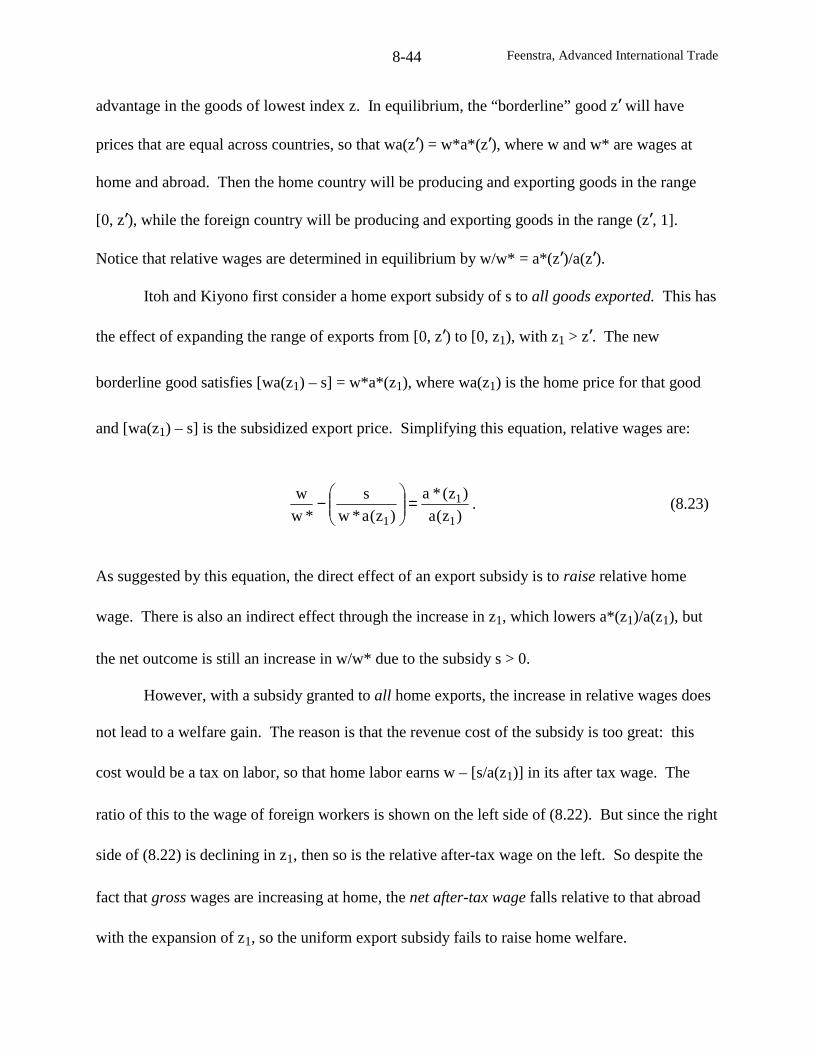
Feenstra, Advanced International Trade8-44
advantage in the goods of lowest index z. In equilibrium, the “borderline” good z’ will have
prices that are equal across countries, so that wa(z’) = w*a*(z’), where w and w* are wages at
home and abroad. Then the home country will be producing and exporting goods in the range
[0, z’), while the foreign country will be producing and exporting goods in the range (z’, 1].
Notice that relative wages are determined in equilibrium by w/w* = a*(z’)/a(z’).
Itoh and Kiyono first consider a home export subsidy of s to all goods exported. This has
the effect of expanding the range of exports from [0, z’) to [0, z1), with z1 > z’. The new
borderline good satisfies [wa(z1) – s] = w*a*(z1), where wa(z1) is the home price for that good
and [wa(z1) – s] is the subsidized export price. Simplifying this equation, relative wages are:
)z(a
)z(*a
)z(a*w
s
*w
w
1
1
1=
− . (8.23)
As suggested by this equation, the direct effect of an export subsidy is to raise relative home
wage. There is also an indirect effect through the increase in z1, which lowers a*(z1)/a(z1), but
the net outcome is still an increase in w/w* due to the subsidy s > 0.
However, with a subsidy granted to all home exports, the increase in relative wages does
not lead to a welfare gain. The reason is that the revenue cost of the subsidy is too great: this
cost would be a tax on labor, so that home labor earns w – [s/a(z1)] in its after tax wage. The
ratio of this to the wage of foreign workers is shown on the left side of (8.22). But since the right
side of (8.22) is declining in z1, then so is the relative after-tax wage on the left. So despite the
fact that gross wages are increasing at home, the net after-tax wage falls relative to that abroad
with the expansion of z1, so the uniform export subsidy fails to raise home welfare.
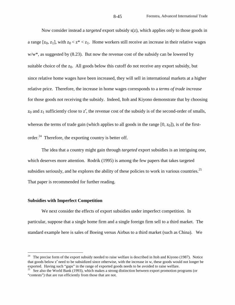
Feenstra, Advanced International Trade8-45
Now consider instead a targeted export subsidy s(z), which applies only to those goods in
a range [z0, z1], with z0 < z* < z1. Home workers still receive an increase in their relative wages
w/w*, as suggested by (8.23). But now the revenue cost of the subsidy can be lowered by
suitable choice of the z0. All goods below this cutoff do not receive any export subsidy, but
since relative home wages have been increased, they will sell in international markets at a higher
relative price. Therefore, the increase in home wages corresponds to a terms of trade increase
for those goods not receiving the subsidy. Indeed, Itoh and Kiyono demonstrate that by choosing
z0 and z1 sufficiently close to z’, the revenue cost of the subsidy is of the second-order of smalls,
whereas the terms of trade gain (which applies to all goods in the range [0, z0]), is of the first-
order.24 Therefore, the exporting country is better off.
The idea that a country might gain through targeted export subsidies is an intriguing one,
which deserves more attention. Rodrik (1995) is among the few papers that takes targeted
subsidies seriously, and he explores the ability of these policies to work in various countries.25
That paper is recommended for further reading.
Subsidies with Imperfect Competition
We next consider the effects of export subsidies under imperfect competition. In
particular, suppose that a single home firm and a single foreign firm sell to a third market. The
standard example here is sales of Boeing versus Airbus to a third market (such as China). We
24 The precise form of the export subsidy needed to raise welfare is described in Itoh and Kiyono (1987). Noticethat goods below z’ need to be subsidized since otherwise, with the increase in w, these goods would not longer beexported. Having such “gaps” in the range of exported goods needs to be avoided to raise welfare.25 See also the World Bank (1993), which makes a strong distinction between export promotion programs (or“contests”) that are run efficiently from those that are not.
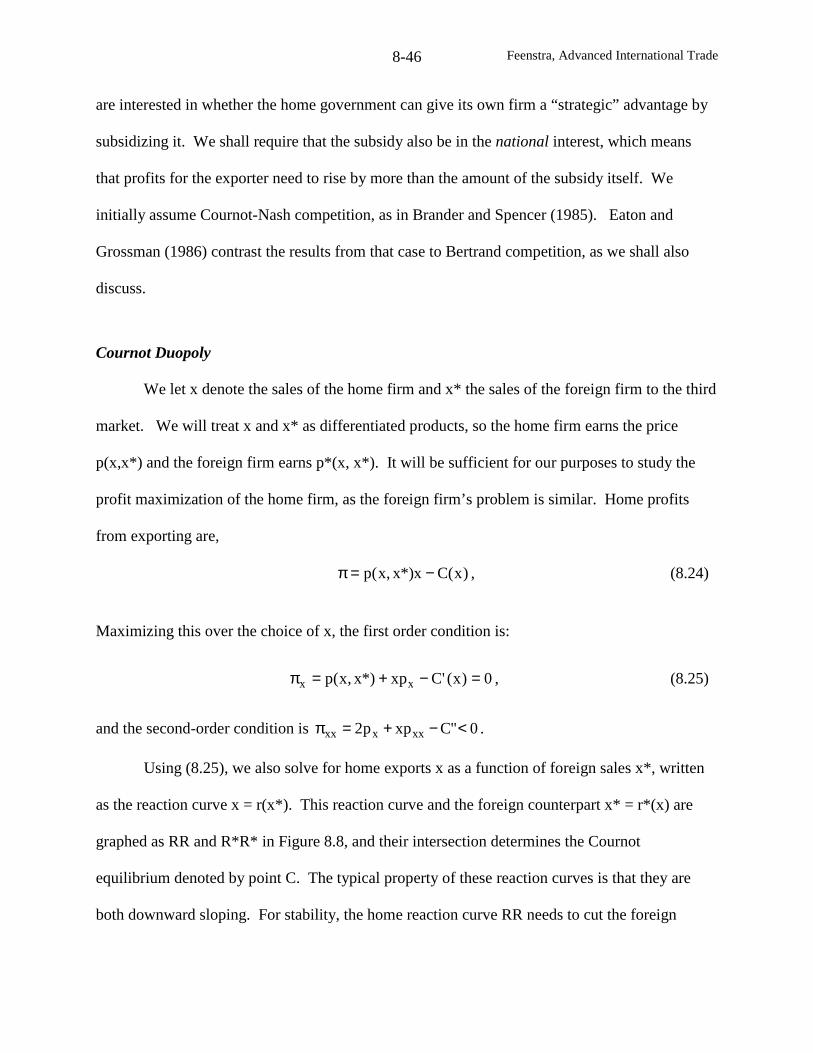
Feenstra, Advanced International Trade8-46
are interested in whether the home government can give its own firm a “strategic” advantage by
subsidizing it. We shall require that the subsidy also be in the national interest, which means
that profits for the exporter need to rise by more than the amount of the subsidy itself. We
initially assume Cournot-Nash competition, as in Brander and Spencer (1985). Eaton and
Grossman (1986) contrast the results from that case to Bertrand competition, as we shall also
discuss.
Cournot Duopoly
We let x denote the sales of the home firm and x* the sales of the foreign firm to the third
market. We will treat x and x* as differentiated products, so the home firm earns the price
p(x,x*) and the foreign firm earns p*(x, x*). It will be sufficient for our purposes to study the
profit maximization of the home firm, as the foreign firm’s problem is similar. Home profits
from exporting are,
)x(Cx*)x,x(p −=π , (8.24)
Maximizing this over the choice of x, the first order condition is:
0)x('Cxp*)x,x(p xx =−+=π , (8.25)
and the second-order condition is 0"Cxpp2 xxxxx <−+=π .
Using (8.25), we also solve for home exports x as a function of foreign sales x*, written
as the reaction curve x = r(x*). This reaction curve and the foreign counterpart x* = r*(x) are
graphed as RR and R*R* in Figure 8.8, and their intersection determines the Cournot
equilibrium denoted by point C. The typical property of these reaction curves is that they are
both downward sloping. For stability, the home reaction curve RR needs to cut the foreign
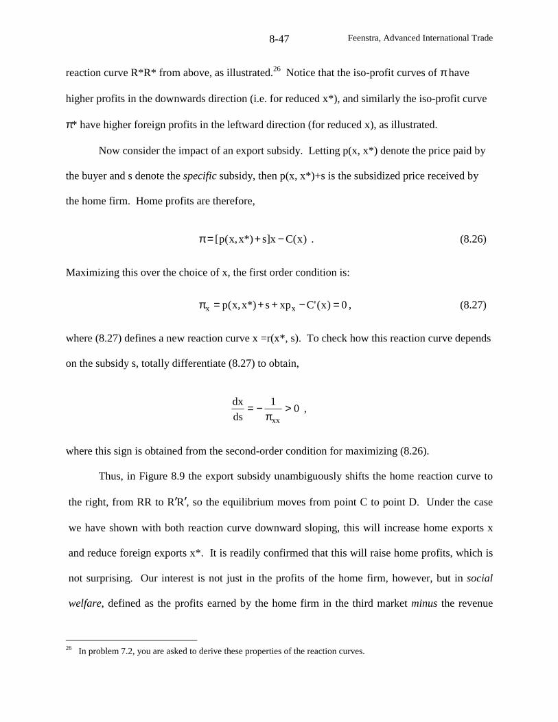
Feenstra, Advanced International Trade8-47
reaction curve R*R* from above, as illustrated.26 Notice that the iso-profit curves of πhave
higher profits in the downwards direction (i.e. for reduced x*), and similarly the iso-profit curve
π* have higher foreign profits in the leftward direction (for reduced x), as illustrated.
Now consider the impact of an export subsidy. Letting p(x, x*) denote the price paid by
the buyer and s denote the specific subsidy, then p(x, x*)+s is the subsidized price received by
the home firm. Home profits are therefore,
)x(Cx]s*)x,x(p[ −+=π . (8.26)
Maximizing this over the choice of x, the first order condition is:
0)x('Cxps*)x,x(p xx =−++=π , (8.27)
where (8.27) defines a new reaction curve x =r(x*, s). To check how this reaction curve depends
on the subsidy s, totally differentiate (8.27) to obtain,
01
ds
dx
xx>
π−= ,
where this sign is obtained from the second-order condition for maximizing (8.26).
Thus, in Figure 8.9 the export subsidy unambiguously shifts the home reaction curve to
the right, from RR to R’R’, so the equilibrium moves from point C to point D. Under the case
we have shown with both reaction curve downward sloping, this will increase home exports x
and reduce foreign exports x*. It is readily confirmed that this will raise home profits, which is
not surprising. Our interest is not just in the profits of the home firm, however, but in social
welfare, defined as the profits earned by the home firm in the third market minus the revenue
26 In problem 7.2, you are asked to derive these properties of the reaction curves.
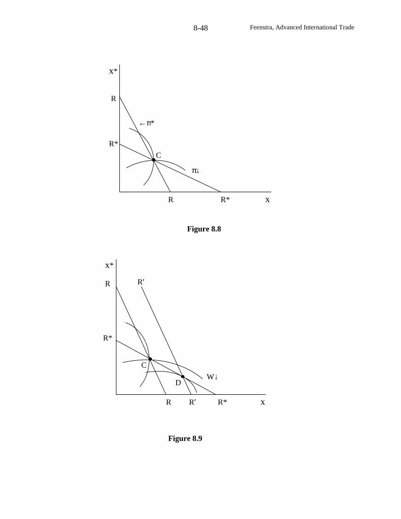
Feenstra, Advanced International Trade8-48
x*
R
R*
←π*
π↓
R R* x
Figure 8.8
W↓
R′
D
C
R R′ R* x
x*
R
R*
Figure 8.9
C
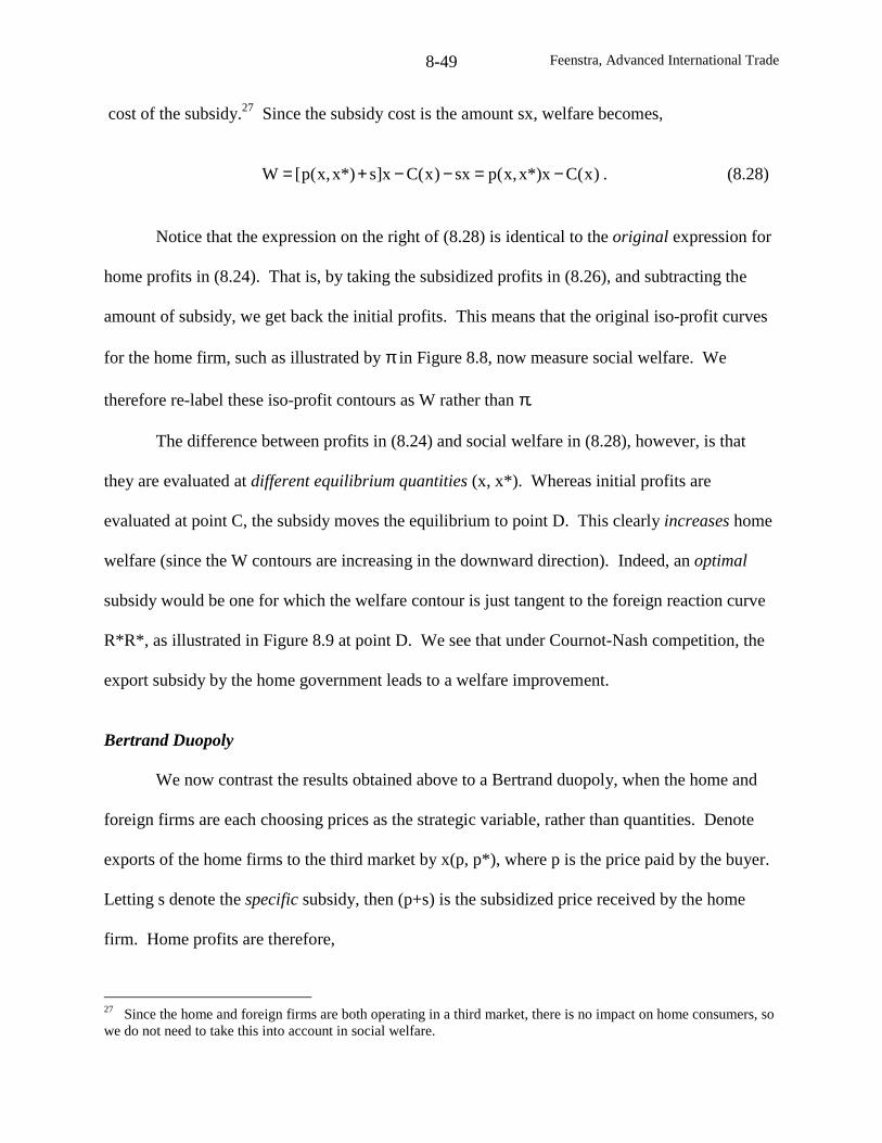
Feenstra, Advanced International Trade8-49
cost of the subsidy.27 Since the subsidy cost is the amount sx, welfare becomes,
)x(Cx*)x,x(psx)x(Cx]s*)x,x(p[W −=−−+= . (8.28)
Notice that the expression on the right of (8.28) is identical to the original expression for
home profits in (8.24). That is, by taking the subsidized profits in (8.26), and subtracting the
amount of subsidy, we get back the initial profits. This means that the original iso-profit curves
for the home firm, such as illustrated by π in Figure 8.8, now measure social welfare. We
therefore re-label these iso-profit contours as W rather than π.
The difference between profits in (8.24) and social welfare in (8.28), however, is that
they are evaluated at different equilibrium quantities (x, x*). Whereas initial profits are
evaluated at point C, the subsidy moves the equilibrium to point D. This clearly increases home
welfare (since the W contours are increasing in the downward direction). Indeed, an optimal
subsidy would be one for which the welfare contour is just tangent to the foreign reaction curve
R*R*, as illustrated in Figure 8.9 at point D. We see that under Cournot-Nash competition, the
export subsidy by the home government leads to a welfare improvement.
Bertrand Duopoly
We now contrast the results obtained above to a Bertrand duopoly, when the home and
foreign firms are each choosing prices as the strategic variable, rather than quantities. Denote
exports of the home firms to the third market by x(p, p*), where p is the price paid by the buyer.
Letting s denote the specific subsidy, then (p+s) is the subsidized price received by the home
firm. Home profits are therefore,
27 Since the home and foreign firms are both operating in a third market, there is no impact on home consumers, sowe do not need to take this into account in social welfare.
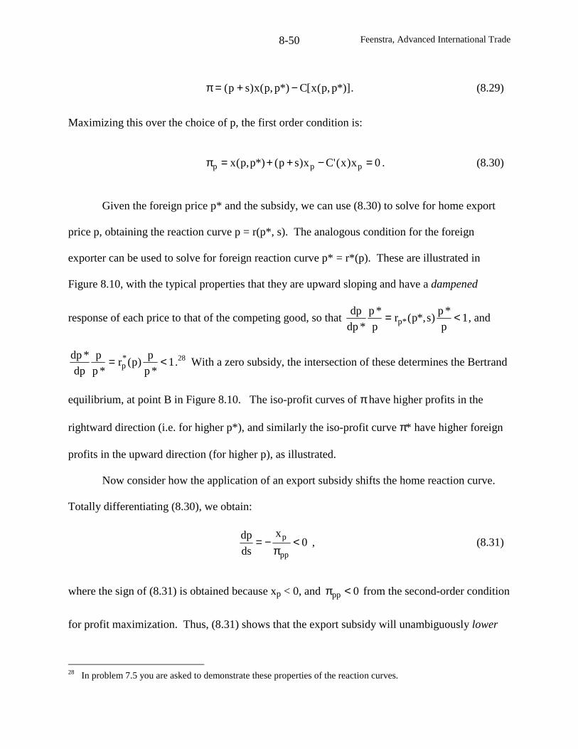
Feenstra, Advanced International Trade8-50
*)]p,p(x[C*)p,p(x)sp( −+=π . (8.29)
Maximizing this over the choice of p, the first order condition is:
0x)x('Cx)sp(*)p,p(x ppp =−++=π . (8.30)
Given the foreign price p* and the subsidy, we can use (8.30) to solve for home export
price p, obtaining the reaction curve p = r(p*, s). The analogous condition for the foreign
exporter can be used to solve for foreign reaction curve p* = r*(p). These are illustrated in
Figure 8.10, with the typical properties that they are upward sloping and have a dampened
response of each price to that of the competing good, so that 1p
*p)s*,p(r
p
*p
*dp
dp*p <= , and
1*p
p)p(r
*p
p
dp
*dp *p <= .28 With a zero subsidy, the intersection of these determines the Bertrand
equilibrium, at point B in Figure 8.10. The iso-profit curves of πhave higher profits in the
rightward direction (i.e. for higher p*), and similarly the iso-profit curve π* have higher foreign
profits in the upward direction (for higher p), as illustrated.
Now consider how the application of an export subsidy shifts the home reaction curve.
Totally differentiating (8.30), we obtain:
0x
ds
dp
pp
p <π
−= , (8.31)
where the sign of (8.31) is obtained because xp < 0, and 0pp <π from the second-order condition
for profit maximization. Thus, (8.31) shows that the export subsidy will unambiguously lower
28 In problem 7.5 you are asked to demonstrate these properties of the reaction curves.
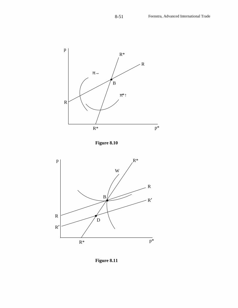
Feenstra, Advanced International Trade8-51
R
p
p*R*
π→
B
R
R*
π*↑
Figure 8.11
Figure 8.10
p*
p
R
R’
R
R’
R*
R*
B
W
D
Feenstra, Advanced International Trade8-52
the price charged by the home firm for its exports (given the foreign price). In Figure 8.11, the
equilibrium is moved from point B to a point like D.
To see how this affects home welfare, we again subtract the cost of the subsidy from
(8.29) to obtain home welfare,
*)].p,p(x[C*)p,p(px*)p,p(sx*)]p,p(x[C*)p,p(x)sp(W −=−−+= (8.32)
In (8.32), we once again obtain a measure of welfare that is identical to home profits in the
absence of the export subsidy. This is shown by the is-profit curve labeled π in Figure 8.10 and
W in Figure 8.11, and increases in the rightward direction, i.e. when the foreign price p*
increases. It is clear from Figure 8.11 that the export subsidy, by leading to a fall in prices, has
reduced home welfare. The reason is that any increase in home profits – measured inclusive of
the subsidy – is more than offset by the revenue cost of the subsidy, so that profits measured
without the subsidy – which equals welfare – has declined.
In order for the home country to gain from and export policy, it must instead impose an
export tax rather than a subsidy. This would have the effect of moving the equilibrium into the
shaded region in Figure 8.11, and raising home welfare due to the increase in prices. These
results are summarized with:
Theorem (Brander and Spencer, 1985, Eaton and Grossman, 1986)
(a) Under Cournot duopoly, a subsidy to exports raises home welfare;
(b) Under Bertrand duopoly, a tax on exports raises home welfare.
Part (b) due to Eaton and Grossman (1986) shows that any “strategic” use of export subsidies is
extremely sensitive to the form of competition. Since we do not expect the government to be
Feenstra, Advanced International Trade8-53
able to distinguish the market conduct, it becomes impossible to implement these policies in a
welfare-improving manner. Furthermore, even if the government knew that a market was
operating under Bertrand competition, the home firm would generally oppose this policy, and in
practice export taxes are rarely used.29
Eaton and Grossman have extended this theorem to discuss other forms of market
conduct, which we do not cover. Regardless of the form of competition, however, there are at
least four other reasons why export subsidies should not be expected to generate a welfare
improvement. First, as we found with a tariff, the possible gains for the home country can be
dissipated by free entry into the industry, so that profits are reduced to zero. This was
demonstrated by Horstmann and Markusen (1986).
Second, we have assumed above that the home exporter takes the subsidy as exogenous,
i.e. the government sets the export subsidy in the first stage of the game, with the home and
foreign firm competing in the second. But Carmichael (1987) argues that in the case of
financing for export credits (such as provided by the U.S. Export-Import bank to purchasers of
U.S. produced aircraft), these subsidies should instead be viewed as endogenous: the
government essentially guarantees a low interest rate to the buyers of aircraft in the second stage
of the game, with firms optimizing over price in the first stage. In that case, McCallum shows
that even under Cournot competition the export subsidies no longer improve welfare. This
result is similar in spirit to what we found in the previous chapter for anti-dumping duties, which
fail to be welfare improving for the importing country when the foreign exporter treats them as
endogenous.
29 An interesting exception is the tax applied to U.S. exports of cotton in the Antebellum period, as discussed byIrwin (2002).
Feenstra, Advanced International Trade8-54
Third, even if the above concerns do not apply, the foreign country could very well
respond by applying subsidies of its own. In that way, the two exporters end up in a “subsidy
war,” which lowers welfare for both of them but raises welfare for the importing country.30 Of
course, this concern also arises with tariffs, where a tariff applied by one country can invite
retaliation by the foreign country and both countries can loose from this tariff war. This will be
discussed in more detail in the next chapter.
Finally, it may well be the case that exporters differ in their productivities, which are not
observable to the government. Brainard and Martimort (1997) have analyzed this in the context
of Cournot competition between home and foreign exporters. With multiple home exporters, the
home government needs to design a subsidy policy that induces them to truthfully reveal their
productivities. It turns out that only the most efficient firms receive subsidies in this case,
whereas the least efficient may very well be taxed.
Conversely, there are several reasons why export subsidies may be welfare improving
regardless of the form of market conduct. Subsidies are often given to R&D rather than exports.
Since R&D is a fixed cost which a firm must incur, these subsidies will influence the decision of
a firm to enter the market or not. Dixit and Kyle (1985) investigate export subsidies in a model
where these may deter entry by foreigners and encourage domestic entry, and find that they
may be beneficial. Related to this, Maggi (1996) investigates subsidies to capacity rather than
exports, in a model that is general enough to include both Bertrand and Cournot competition.
He finds that these subsidies are weakly welfare improving, i.e. they will raise or leave
unchanged welfare of the exporting country. Finally, export subsidies may be used in markets
where learning is important, so that costs fall over time. This is the case in the manufacture of
30 See problem 8.5.

Feenstra, Advanced International Trade8-55
semiconductors, for example, and also aircraft.31 Then similar to the infant-industry argument
for a tariff, subsidies may possibly be welfare improving.
Subsidies to Commercial Aircraft
A favorite industry to study the impact of export subsidies is aircraft. In large passenger
aircraft, there have been just three competitors: Boeing and McDonnell-Douglas in the U.S. and
Airbus in Europe. The former two companies merged on August 1, 1997, so the industry
effectively became a duopoly. Various types of subsidies have been used in both the U.S. and
Europe to support their respective firms, so this is an ideal case to evaluate the theoretical results
described above.
The idea that the two countries can be is a “subsidy war” appears to apply in this
industry. Recognizing this, the U.S. and the Europe Community reached an agreement in 1992,
which limited subsidies to 33% of development costs (see Tyson, 1992, and Pavcnik, 2002). In
addition, the agreement prohibits production subsidies and limits the ability of government
agencies to subsidize the interest rate on purchases of aircraft. Irwin and Pavcnik (2001) find
that as a result of this accord, prices for commercial aircraft rose by something between 3.1%
and 8.8%. They estimate that the reduction in subsidies granted is somewhat higher than this
amount – between 7.5% and 12.5%.
There are recent claims that the terms of the 1992 agreement are being violated by a new
aircraft under development by Airbus. As described by Irwin and Pavcnik (2001), commercial
aircraft are comprised of two distinct product types: narrow-body aircraft with a single aisle,
including the Boeing 737, 757 and Airbus A-320; and wide-body aircraft with two aisles,
31 A simulation model of subsidies to aircraft is presented by Baldwin and Krugman (1988b), and the dynamics ofproduction and sales in this industry are estimated by Benkard (2000a,b,).
Feenstra, Advanced International Trade8-56
including the Boeing 747, 777 and Airbus A-300. Airbus has now announced plans for the
production of another wide-body aircraft, the A-380, which will be even larger than the Boeing
747 and will compete directly with the 747 in long flights. The expenditures to develop the A-
380 are estimated to be $12 billion, of which the governments of France, Germany, the
Netherlands, Belgium, Spain, Finland, and the U.K. are expected to cover up to one-third. This
subsidy has led to a trade dispute between the U.S. and Europe over whether financing of the A-
380 violates the 1992 agreement, as described in Pavcnik (2002).
The goal of Irwin and Pavcnik (2001) is to estimate demand and markups for wide-body
aircraft, and then simulate the effect of A-380 entry on the market equilibrium. Airbus has stated
that it needs to produce at least 250 planes to cover the development costs, but that it expects to
sell 1,500 aircraft over the next 20 years. It has received initial orders for 60 planes (as of early
2001), but these appear to have received a discount of at least 10%, and perhaps as high as 35%,
off the list price of $235 million per plane. Boeing, on the other hand, states that market demand
for such a super jumbo will not exceed 700 aircraft over the next 20 years. We can expect the
estimation of market demand and prices, and the simulation of A-380 entry, to inform us as to
which projection (700 planes or 1,500 planes) is more accurate.
Demand for a differentiated product depends on the quality-adjusted prices, which we
wrote earlier as qi = pi/f(zi). Suppose that we instead measure quality-adjusted prices qi by the
difference between nominal prices pi and quality f(zi). In addition, we assume that quality is a
linear function of characteristics, so the quality-adjusted prices become qj = αpj – β’zj – ξj. In
this notation, ξj reflects unmeasured characteristics of product j, which we treat as a random
variable. Then the logit specification of demand is:
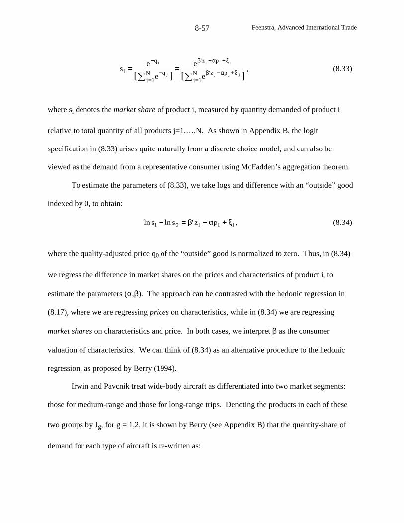
Feenstra, Advanced International Trade8-57
][][ N1j
pz'
pz'
N1j
q
q
ijjj
iii
j
i
e
e
e
es
∑∑ =ξ+α−β
ξ+α−β
=−
−== , (8.33)
where si denotes the market share of product i, measured by quantity demanded of product i
relative to total quantity of all products j=1,…,N. As shown in Appendix B, the logit
specification in (8.33) arises quite naturally from a discrete choice model, and can also be
viewed as the demand from a representative consumer using McFadden’s aggregation theorem.
To estimate the parameters of (8.33), we take logs and difference with an “outside” good
indexed by 0, to obtain:
iii0i pz'slnsln ξ+α−β=− , (8.34)
where the quality-adjusted price q0 of the “outside” good is normalized to zero. Thus, in (8.34)
we regress the difference in market shares on the prices and characteristics of product i, to
estimate the parameters (α,β). The approach can be contrasted with the hedonic regression in
(8.17), where we are regressing prices on characteristics, while in (8.34) we are regressing
market shares on characteristics and price. In both cases, we interpret β as the consumer
valuation of characteristics. We can think of (8.34) as an alternative procedure to the hedonic
regression, as proposed by Berry (1994).
Irwin and Pavcnik treat wide-body aircraft as differentiated into two market segments:
those for medium-range and those for long-range trips. Denoting the products in each of these
two groups by Jg, for g = 1,2, it is shown by Berry (see Appendix B) that the quantity-share of
demand for each type of aircraft is re-written as:
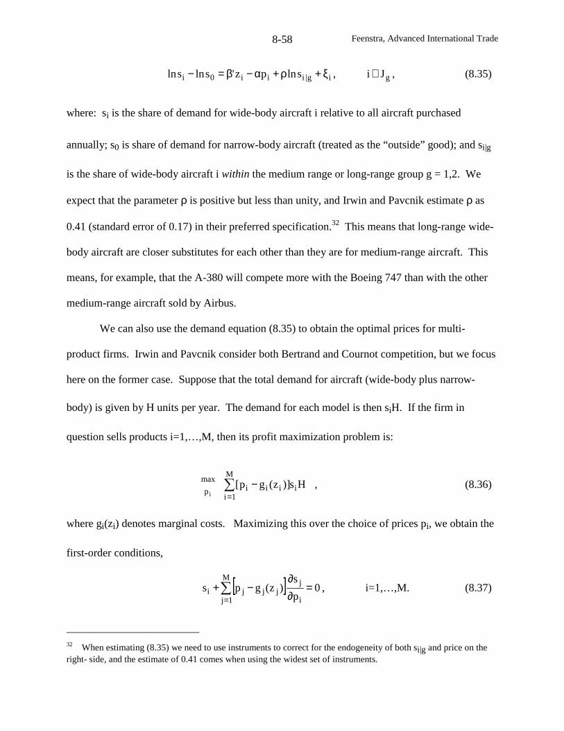
Feenstra, Advanced International Trade8-58
ig|iii0i slnpz'slnsln ξ+ρ+α−β=− , gJi ∈ , (8.35)
where: si is the share of demand for wide-body aircraft i relative to all aircraft purchased
annually; s0 is share of demand for narrow-body aircraft (treated as the “outside” good); and si|g
is the share of wide-body aircraft i within the medium range or long-range group g = 1,2. We
expect that the parameter ρ is positive but less than unity, and Irwin and Pavcnik estimate ρ as
0.41 (standard error of 0.17) in their preferred specification.32 This means that long-range wide-
body aircraft are closer substitutes for each other than they are for medium-range aircraft. This
means, for example, that the A-380 will compete more with the Boeing 747 than with the other
medium-range aircraft sold by Airbus.
We can also use the demand equation (8.35) to obtain the optimal prices for multi-
product firms. Irwin and Pavcnik consider both Bertrand and Cournot competition, but we focus
here on the former case. Suppose that the total demand for aircraft (wide-body plus narrow-
body) is given by H units per year. The demand for each model is then siH. If the firm in
question sells products i=1,…,M, then its profit maximization problem is:
∑=
−M
1iiiiip
maxHs)]z(gp[
i, (8.36)
where gi(zi) denotes marginal costs. Maximizing this over the choice of prices pi, we obtain the
first-order conditions,
[ ] 0p
s)z(gps
M
1j i
jjjji =
∂∂
−+∑=
, i=1,…,M. (8.37)
32 When estimating (8.35) we need to use instruments to correct for the endogeneity of both si|g and price on theright- side, and the estimate of 0.41 comes when using the widest set of instruments.
Feenstra, Advanced International Trade8-59
To simplify this expression, the derivatives of the market shares can be calculated from (8.35),
and substituted into (8.37). In addition, we suppose that marginal costs are linear in
characteristics, so gi(zi) = γ’zi + ωi, where ωi is a random error.
Irwin and Pavcnik (2001) estimate the demand parameters from (8.35), and substitute
these into (8.37) in order to compute the markups. They find that these markups are high:
current prices are about twice as high as marginal costs (under either Bertrand or Cournot
competition), and even higher in past years. Having obtained estimates of demand and markups,
they then simulate the effect of A-380 entry into the market. On the demand side, we know that
this plane will be a close substitute for other long-range, wide-body aircraft such as the Boeing
747. But on the pricing side, having multi-product firms means that Airbus will be less
concerned than Boeing about the entry of this new product stealing demand away from its
existing products. That is, Boeing will respond more aggressively than Airbus in lowering its
own prices to prevent market share from falling (since Airbus is happy to have demand shifted
towards its own new product). These predictions are borne out in the simulations. Relative to
their previous sales, the percentage decline in demand is smaller for Boeing than for Airbus,
because Boeing responds more aggressively in cutting its prices. Nevertheless, including the
new sales of A-380, the overall market share of Airbus increases.
How many of the new A-380’s will Airbus sell? This depends, of course, on the price
charged. Irwin and Pavcnik experiment with discounts from the list price of 0 – 30%. With the
largest discount, they calculate that Airbus will sell 34 planes annually, or 680 over 20 years,
yielding $110 billion in revenues. But annual sales of the A-380 are only one-half (one-quarter)
as much when discounts of 20% (10%) are used instead, indicating that demand for the A-380 is
Feenstra, Advanced International Trade8-60
highly elastic. High markups in this market are sustained because firms are selling multiple
products, but at the full list price for the A-380 its demand is extremely low – only 4 or 5 planes
annually, which would not cover development costs. Lack of detailed cost data means that we
cannot estimate the profit-maximizing price for the A-380, but it is evident that high discounts
are needed to achieve significant sales. Even with the 30% discount, however, demand falls well
below the market projection of 1,500 planes made by Airbus. Rather, sales at that discount are
closer to the 700 planes expected by Boeing, whose company representatives state that demand
at that level will not allow the project to be profitable.
Conclusions
In the previous chapter, we identified three effects of a tariff on welfare: (i) a deadweight
loss; (ii) a terms of trade effect; (iii) a reduction in the monopoly distortion if the output of home
firms increase (without leading to inefficient entry). While we have not derived again the
welfare criterion for an import quota, a similar decomposition would apply. However, any
potential terms of trade gain becomes a loss if the importing country gives up the quota rents to
the exporter, as under a VER. In that case, the only possible source of gain for the importing
country would be under effect (iii), if the import quota led to a significant increase in home
output and offset a monopoly distortion. But we have found that the reverse case is more likely
to hold: with either a home monopoly or Bertrand duopoly, the quota (say, at the free trade level
of imports) will lead to an increase in price and reduction in home quantity, so that the monopoly
distortion is worsened rather than offset.
For export subsidies under perfect competition, the welfare criterion becomes: (i) a
deadweight loss; (ii) a terms of trade effect. Whereas the terms of trade will improve due to a
tariff for a large country, it will instead worsen due to the export subsidy in a two-good model.
Feenstra, Advanced International Trade8-61
We have noted, however, that with more goods there is the possibility that a subsidy on some
goods will raise the terms of trade for others. The Ricardian model with a continuum of goods
provides a good illustration of this, and allowed for welfare-improving export subsidies when
they are targeted on a narrow range of goods. Determining whether this has occurred in any
actual cases would be an interesting area for further research.
Under imperfect competition, the welfare criterion is simplified by considering sales to a
third market. In that case the home firm earns profits from its export sales, and welfare is simply
the difference between these and the revenue cost of the subsidy. This provides the clearest
example of a potential role for “strategic” trade policy in shifting profits towards the home firm.
As we have seen, however, subsidies may or may not be desirable: under Cournot competition
export subsidies raise welfare, but under Bertrand competition they do not. Since it is very
difficult to know the type of competition being used by firms, it becomes impossible for the
government to implement this policy in a welfare-improving manner.
Empirically, the analysis of import quotas and export subsidies are linked because the
industries involved are often producing discrete products, with multi-product firms. This chapter
has served as an introduction to the empirical techniques that can be used on such industries,
including hedonic regressions and the estimation of demand and prices as in Berry (1994). The
reader is referred to Appendix B for more details on discrete choice methods, which should be
useful for many trade policy issues.
Feenstra, Advanced International Trade8-62
Problems
8.1 Suppose that the home and foreign firms are engaged in Cournot competition in the home
market. Illustrate the free trade equilibrium, and answer:
a) Suppose that a VER is negotiated with the foreign firm, so that it agrees to not sell more than
its free-trade quantity. What is the effect on the equilibrium?
b) Suppose that the VER is negotiated at below the free trade quantity. Show the effect on the
equilibrium.
8.2 Suppose that the home firms and foreign firm are initially engaged in Bertrand competition
in the home market, as discussed in the text. Suppose that the VER is negotiated at below the
free trade quantity. Show the effect on the equilibrium and on profits.
8.3 Building on problem 5.3 in chapter 5, consider the CES utility function written as in (8.2),
σ−σ=θ= ∑=
θ /)1(,caUN
1iii ,
where ai = f(zi)θ
is a transformation of the quality of each product, and can be treated as a
parameter, i=1,…,N.
(a) Maximize this subject to the budget constraint, Icp iiN
1i ≤∑ = , to obtain an expression
for the demands ci as a function of prices and income.
(b) Use these expressions to show that .ji,p/cp/c ijji ≠∂∂=∂∂
(c) Also show that equation (8.9) holds, which we re-write as:
σ−+σ=
∂∂− ∑∑
==
M
1j
jjM
1j j
i
I
cp)1(
pln
cln.
Feenstra, Advanced International Trade8-63
8.4 Consider the problem of maximizing profits subject to the VER constraint in (8.11). Using
the same steps as in (8.6) to (8.9), show that the solution for prices is as in equation (8.15).
8.5 Consider a Cournot duopoly exporting to a third market, and suppose that both countries
apply export subsidies. Illustrate where this “subsidy war” can end up, i.e. illustrate the Nash
equilibrium in subsidies for both governments.

Feenstra, Advanced International Trade8-64
Empirical Exercise
This exercise is to reproduce regression results Feenstra (1988a). To complete the exercise, the
files “car_7990.dta, truck_7990.dta” should be stored in: c:\Empirical_Exercise\Chapter_8\.
Then do:
8.1 Run the programs “pindex_c.do, pindex_t.do, unit_value.do” to reproduce the price indexes
and unit-values for cars and trucks in Table 8.3. What formula is used for the price indexes, and
how do these differ from the unit-values?
8.2 Run the program “car_reg.do” to reproduce the column (1) in Table 8.4, and the program
“truck_reg.do” to reproduce column (2). What weights are being used in the regression, and
how does this affect the results?
8.3 Pooling car and truck data, run “system_7985.do” to reproduce columns (3) and (4) in Table
8.4 with the constraints specified in equation (8.22). How are these constraints built into the
program for the nonlinear regression?
8.4 Run the programs “unit_quality.do, qindex_c.do, qindex_t.do” to reproduce the quality
indexes and unit-qualities for cars and trucks in Table 8.3. What formula is used for the quality
of each model and the quality indexes, and how do these differ from the unit-qualities?
8.5 Pooling car and truck data, run “system_nocom.do” and “system_wcon.do” to reproduce
columns (1) – (4) in Table 8.5, with constraints specified in equation (8.22).

Feenstra, Advanced International Trade
Chapter 9 – Political Economy of Trade Policy
In the previous two chapters we have covered the basic analysis of trade policies,
including models of imperfect competition. The idea that non-competitive markets give rise to
opportunities for governments to gain from trade policies has been an important line of research.
It has ultimately been concluded, however, that such opportunities for “strategic” use of trade
policy are very limited. This raises the obvious question of why trade policies are used so often?
One answer is that such policies are politically motivated: tariffs are granted in response to
demands by special interest groups, such as industries and unions. The research issue is to
understand how such demands are mediated through the political process. In this chapter we
outline research on the political economy of protection, including the median voter model of
Mayer (1984) and the “protection for sale” model of Grossman and Helpman (1994).
The “protection for sale” model has been extended in a number of directions. Mitra
(1999) has shown how to introduce endogenous lobbies into that framework, as we shall discuss.
Grossman and Helpman (1995a) further use this framework to analyze a tariff war between two
countries, and the potential benefits from international agreements. Along the same lines,
Bagwell and Staiger (1999, 2002) examine the economic rationale for the trade rules embodied
in the General Agreement on Trade and Tariffs (GATT) and the World Trade Organization
(WTO). These rules include GATT’s principle of “reciprocity,” whereby each country agrees to
reduce its trade barriers in return for a reciprocal reduction by another. Bagwell and Staiger’s
framework is general enough to include both the median voter model and the “protection for
sale” model, and we use it to show the outcome of a trade war, along with the benefits from
reciprocal tariff reductions using GATT rules.
Feenstra, Advanced International Trade9-2
Another importance principle of GATT is the “most favored nation” (MFN) provision,
which states that all member countries of GATT should be granted the same tariffs. This
provision is violated when countries join into regional trade agreements, granting zero tariffs to
countries within but not outside the agreement. Our third topic is to examine the incentives for
countries to join regional trade agreements versus multilateral agreements. A key question here,
raised by Bhagwati (1993), is whether joining a regional trade agreement helps or hinders the
ultimate goal of multilateral free trade. Models indicating that regional agreements may hinder
multilateral free trade include Krishna (1998) and McLaren (2002), and views on the other side
include Baldwin (1995) and Ethier (1998). We will examine this issue using the median voter
model, as in Levy (1997). In the basic version of this model a regional agreement cannot hinder
a multilateral agreement, but in an extended version of the model this can occur.
We conclude the chapter with an application of political economy to a non-democratic
setting: the People’s Republic of China. In this case the special interest groups do not take the
form of well-funded lobbying groups as in the U.S., but rather, include the large state-owned
industries and the smaller but growing private industries, as well as foreign firms. The
distribution of these firms is very uneven across provinces. China’s recent entry into the WTO
came only after regional concerns in China about the impact of import competition were
overruled. We argue that the regional variation towards openness (as evidenced by the inflow of
foreign firms), combined with the variation in location of state-owned firms, can be used to
identify the political weights given to the various interest groups. We present the results of
Branstetter and Feenstra (2002), which show how the Grossman-Helpman framework can be
applied in this setting.
Feenstra, Advanced International Trade9-3
Median Voter Model
Used in many applications, the median voter model presumes that policies are established
by majority vote. Provided that preferences are “single peaked” over the policy being voted
upon (i.e. each person has a unique maximum), then it follows that the policy adopted will
maximize the utility of the median voter. In the application to trade policy we assume that the
policy is an import tariff or subsidy. The optimal tariff for the median voter will depend on the
production structure in the economy, and for simplicity in this section we assume the two-by-two
Heckscher-Ohlin (HO) model (Mayer, 1984, also considers other structures). Then we will show
that if the median voter owns a lower capital/labor ratio than overall for the economy, and
imports are labor-intensive, the economy will have a positive import tariff.
As in chapter 7, we will suppose that each individual has a quasi-linear utility function
given by )c(Uc hh0 + , where h
0c is consumption of a numeraire export good, and ch
is the
consumption of the import good for consumer h=1,…,L. (We use L rather than H to denote the
number of consumers, since L also equals the number of workers). Consumers all have the same
increasing and strictly concave utility function U, so they have the same optimal consumption
ch
= d(p), d’(p) < 0, with remaining income spent on the numeraire good, )p(d'pIc hh0 −= .
Then individual utility is,
)]p(d[U)p(d'pI)I,p(V hh +−≡ . (9.1)
Both the export and import goods are produced using labor and capital. The total
endowments of labor and capital are L and K, respectively. The fixed world price of the import
is denoted by p*, and this good has a specific tariff of t, so the domestic price is p = p* + t. We
let y(p) denote the supply of the import-competing good, with y’(p) > 0. Imports are then m(p) =
Feenstra, Advanced International Trade9-4
d(p)L – y(p), and tariff revenue collected is T = tm(p), which is redistributed with a poll subsidy.
We will suppose that individual h has one unit of labor and Kh
units of capital, h=1,…,L, so that
individual income is, Ih
= w + rKh
+ (T/L). We can re-express this as,
)TrKwL(L
1)TLrKwL(
L
1I hhh +ρ+=++= , (9.2)
where )L/K/(Khh =ρ is the capital/labor ratio for the individual in question relative to the
overall capital/labor ratio in the economy. Total GDP in the economy is G = y0(p) + py(p) =
wL + rK. It follows that we can re-write individual income in (9.2) as:
]T)p(py)p(yrK)1[(L
1]TrK)1(rKwL[
L
1I 0
hhh +++−ρ=+−ρ++= . (9.2’)
Differentiating individual utility in (9.1) with respect to the tariff, we obtain:
,)p('mL
t
L
K
dp
dr)1(
dp
dT
L
1)p(d
L
)p(y
L
K
dp
dr)1(
dt
dI)p(d
dt
dV
h
h
hh
+−ρ=
+
−+−ρ=
+−=
(9.3)
where the first line follows from Roy’s Identity, the second line using (9.2’), and the third line
using tariff revenue of T = t[d(p)L – y(p)] = tm(p).
If the tariff is determined by majority vote, then the tariff prevailing will be that which
maximizes the utility of the median voter. Denoting the median voter by “m,” with utility
Feenstra, Advanced International Trade9-5
),I,p(VV mm = this tariff will satisfy 0dt/dVm = and 0dt/Vd 2m2 < . Setting (9.3) equal to
zero, this tariff is:
)p('m
K
dp
dr)1(t mm ρ−= , (9.4)
where ρmis the capital/labor ratio for the median individual h relative to the overall capital/labor
endowment for the economy. This ratio is less than one for all countries (Alesina and Rodrik,
1994), so that ρm< 1. Then since m’(p) < 0, we see that the tariff t
mis positive when the import
good is labor-intensive, so that dr/dp < 0, but negative when the import good is capital- intensive,
so that dr/dp > 0. In other words, import tariffs should be used in capital-abundant industrialized
countries, but import subsidies in labor-abundant developing countries.
In practice, import subsidies are rarely observed, despite this prediction from the median
voter model. There are many reasons for this, some of which we will investigate later in this
section. Setting aside this most obvious limitation of the median voter model, Dutt and Mitra
(2002) ask whether there is some other prediction that might accord better with real world
evidence. In particular, suppose that we compare countries with varying degrees of inequality,
which we measure by (1–ρm), i.e. with lower values of the median voter’s capital/labor
endowment ρm, corresponding to higher inequality. Then differentiating the first-order condition
0dt
dVm
= , we obtain 0)1(ddt)1(d
Vddt
dt
Vd mm
m2
2
m2
=ρ−ρ−
+ , so that from (9.3):
2
m2
m
m
dt
Vd
L
K
dp
dr
)1(d
dt =ρ−
, (9.5)
Feenstra, Advanced International Trade9-6
where 0dt/Vd 2m2 < from the second-order condition.
It follows that for capital-abundant countries importing the labor-intensive good, so that
dr/dp < 0, the median voter model predicts that increased inequality (a rise in 1–ρm) will lead to
a higher tariff. Conversely, for labor-abundant countries importing the capital-intensive good, so
that dr/dp > 0, the median voter model predicts that increased inequality (a rise in 1–ρm) will
lead to a reduced tariff or increased subsidy (a fall in tm
). Stated less formally, we expect
increased inequality to be associated with more restrictive trade policies in industrialized
countries, but more open trade policies in developing countries.
Dutt and Mitra test this prediction by running the regression:
iii
3ii
2i
10i X)L/K()L/K(INEQINEQTR ε+β+α+α+α+α= , (9.6)
where TRiis an measure of trade restrictions in country i, INEQ
iis an index of income inequality
in that country, (K/L)iis the capital/labor ratio in country i, and X
iis a matrix of other control
variables. Taking the partial derivative of TRiwith respect to INEQ
i, we obtain,
i21i
i
)L/K(INEQ
TR α+α=∂∂
. (9.6’)
The prediction from the median voter is that this derivative should be negative for low levels of
the capital/labor ratio (K/L)i, but positive for higher levels of the capital/labor ratio. This will
occur if α1 < 0 and α2 > 0, with the turning point between the negative and positive derivatives
occurring where (9.6’) equals zero, or at the capital/labor ratio (K/L)i= –α1/α2 > 0.
Feenstra, Advanced International Trade9-7
In their estimates, Dutt and Mitra confirm these signs of α1 and α2 for several different
measures of tariffs used for TRi. The turning point (K/L)
i= –α1/α2 turns out to be quite close
to the median capital/labor ratio in the sample (South Korea). For developing countries with
lower capital/labor ratios, greater inequality leads to lower tariffs. Conversely, for industrialized
countries with higher capital/labor ratios, greater inequality leads to higher tariffs. This provides
striking support for the median voter framework in the context of the Heckscher-Ohlin model. In
addition, Dutt and Mitra find that this relationship holds better in democracies than in
dictatorships.
This confirmation of the median voter model seems at odds with its first prediction, that
tariffs should be positive in advanced countries importing labor-intensive goods, but negative in
developing economies importing capital-intensive goods. As we have mentioned, import
subsidies are rarely observed. Fernandez and Rodrik (1991) provide one explanation for the
“anti-trade” bias of nearly all countries. Specifically, they argue that even if policies are
determined by majority vote, when individuals do not know whether they will be included
among the gainers or losers, there is a tendency for voters to prefer the status quo. This occurs
even in a model where everyone is perfectly informed about the aggregate gains and losses in
each industry, but cannot predict their individual returns. Therefore, there is a tendency to apply
tariffs to offset import competition and preserve the status-quo income distribution.1 This can
help to reconcile the positive tariffs observed in most countries with the median voter model, and
the logic of Fernandez and Rodrik holds equally well in other models, as well.
1 The idea that trade policy is applied to preserve the status-quo income distribution has also been proposed byCordon (1974), and is known as the “conservative social welfare function;” see also Deardorff (1987). In Fernandezand Rodrik (1991), this is the outcome of majority vote rather than a criterion imposed by the government.
Feenstra, Advanced International Trade9-8
Protection for Sale
The median voter model assumes that policies are determined by majority vote. This is
an overly simplified description of representative democracies where the electorate votes for
legislators, who then determine the policies. In such settings the policies chosen will be jointly
influenced by votes, voice, and dollars from the campaign contribution of lobbying groups. The
second model we consider, due to Grossman and Helpman (1994), proposes an elegant solution
to the problem of how the government simultaneously considers the contributions of numerous
lobbies, as well as consumer welfare, in determining trade policy.2
We assume that there are N goods plus the numeraire commodity. On the demand side,
consumer utility functions are ∑ =+ N1i
hii
h0 )c(uc , where h
0c is the numeraire export good, and hic
is the consumption of good i=1,…,N. Maximizing utility subject to the budget constraint gives
the per-capita consumption di(pi) of each good, i=1,…,N, with remaining income spent on the
numeraire good, )p(d'pIc hh0 −= . We let d(p) = [d1(p1),…,dN(pN)] denote the vector of per-
capita consumptions, depending on prices p=(p1,…,pN). Then individual utility is similar to that
in (9.1),
∑=
+−≡N
1iiii
hh )]p(d[u)p(d'pI)I,p(V . (9.7)
Notice that the last two terms on the right of (9.7) give per-capita consumer surplus, or
2 Earlier political economy models, such as Findlay and Wellisz (1982), simply assumed a functional relationshipbetween lobbying contributions and tariffs. Hillman (1989) allowed for a government objective function with ageneral tradeoff between the benefits to a special interest group and costs to consumers of tariff protection. Theadvantage of Grossman and Helpman (1994) is that these functional relationships are endogenously determinedrather than assumed.
Feenstra, Advanced International Trade9-9
)p(d'p)]p(d[u)p(SN
1iiii −≡ ∑
=, so that consumer welfare can be written as:
)p(SI)I,p(V hhh +≡ , (9.7’)
with )p(dp/)p(S iii −=∂∂ , by Roy’s Identity.
On the production side, each of the N industries has the production function yi = fi(Li,Ki),
where capital Ki is specific to each sector. The numeraire commodity is produced with one unit
of labor, so wages are fixed at unity. Given the product price pi in each sector, the return to the
specific factor in that sector is,
]L)K,L(fp[)p( iiiiiiL
maxii −=π . (9.8)
From (9.8) we can determine the optimal outputs )p(y)p( iiii =π′ in each industry. The
international prices of the goods are fixed at *ip , and each industry may receive a specific trade
policy of ti, i=1,…,N, where ti > (<) 0 indicates a tariff (subsidy) in an import industry, and a
subsidy (tariff) in an export industry. Imports of each good are then mi(pi) = di(pi)L – yi(pi)
(which are negative for exports), and tariff revenue collected is ∑ = −= N1i ii
*ii )p(m)pp()p(T .
We assume that this revenue is redistributed by a poll subsidy of (T/L) per person.
The specific factor in each industry i is owned by Hi members of the population, so that
∑ == N1i iHH is the total number of persons owning some capital. For simplicity, we suppose that
every individual also own one unit of labor. The total population is L, so there are an additional
(L – H) > 0 persons who own one unit of labor but no capital. The owners of specific capital in
each industry earn the return )p( iiπ from (9.8), and obtain their wages of unity plus consumer
Feenstra, Advanced International Trade9-10
surplus, along with re-distributed tariff revenue. Summing these various terms, the owners of
specific capital in industry i earn:
)p(T)L/H()]p(S1[H)p()p(W iiiii +++π= , i=1,…,N. (9.9a)
The remaining (L – H) persons obtain their wages plus consumer surplus, and re-distributed
tariff revenue, so their welfare is:
)p(T]L/)HL[()]p(S1)[HL()p(W0 −++−= . (9.9b)
Summing (9.9) over all workers and industries, we obtain total welfare,
)p(T)]p(S1[L)p()p(W)p(W ii
N
1i
N
0ii +++π== ∑∑
==. (9.10)
We suppose that a subset of the industries oJj ∈ are organized into lobbies, while the
complementary set uJj ∈ are unorganized industries, with }.N,...,1{JJ uo =∪ The purpose of
each lobby is to provide contributions to the government in return for influencing the
tariff/subsidy schedule. Specifically, they announce a campaign contribution schedule )p(R j
that they are willing to pay, depending on the vector of prices i*ii tpp += prevailing across the
industries, i=1,…,N. The government values campaign contributions, but also weighs these
against the consumer welfare of all individuals. Giving social welfare the weight of α > 0,
Grossman and Helpman assume that the government chooses tariffs and subsidies ti to maximize,
∑∈
α+=oJj
j )p(W)p(R)p(G . (9.11)
Feenstra, Advanced International Trade9-11
The key question is how the lobbies in industries oJj ∈ determine their campaign
contributions. The answer to this comes from the work of Bernheim and Whinston (1986). They
argue that in the Nash equilibrium of the game we have described – with each lobby optimally
choosing its contribution schedule )p(R j taking as given the schedules of the other groups, and
knowing that the tariffs will be chosen to maximize (9.11) – then the lobbies can do no better
than to select a contribution schedule of the form:
}B)p(W,0{max)p(R jjj −= , oJj ∈ , (9.12)
where Bj is a constant.3 Bernheim and Whinston refer to this as a truthful contribution schedule,
since it reflects the true welfare levels Wj(p) obtained by the lobby for various tariffs. They
argue that a truthful Nash equilibrium, where each lobby uses a schedule like (9.12), is included
among the equilibria of the game.
Accepting this result of Bernheim and Whinston (1986), we can substitute (9.12) into
(9.11) to obtain:
∑∑∉∈
α+−α+=oo Jj
jjJj
j )p(W]B)p(W)1[()p(G , (9.11’)
where the summation over oJj ∉ also include the welfare W0 of workers with no capital. Notice
that this statement of the government’s objective function indicates that it gives differential
weights to the welfare of organized and unorganized industries: the organized lobbies have the
weight (1+α), whereas other industries plus workers have the weight α.
3 Notice that by using the truthful contribution schedules in (9.12), the welfare of each lobby net of the
contributions becomes Wj(p) – Rj(p) = min {Wj(p) , Bj}, so Bj is an upper-bound on net welfare. Grossman and
Helpman (1994, pp. 843-847) discuss how Bj might be determined, as does Mitra (1999).
Feenstra, Advanced International Trade9-12
Choosing the tariffs ti to maximize (9.11’) is equivalent to choosing the domestic prices
pj, oJj ∈ to maximize this. Before computing the first-order condition, we can differentiate
welfare for an organized industry, unorganized industry and workers as:
−+
+−=
∂
∂
j
j*jjj
jjjj
j
j
dp
dm)pp(m
L
H)p(dHy
p
W, for oJj ∈ , (9.12a)
−+
+−=
∂
∂
j
j*jjj
iji
j
i
dp
dm)pp(m
L
H)p(dH
p
W, for uJi ∈ , (9.12b)
−+
−+−−=
∂
∂
j
j*jjjj
j
0
dp
dm)pp(m
L
HL)p(d)HL(
p
W, (9.12c)
where mj = dj(pj)L – yj(pj) is the imports of good j (which is negative for exports).
Then multiply (9.12a) by (1+α), and (9.12b) and (9.12c) by α, and sum these over all
organized and unorganized industries to obtain:
,Jj,dp
dm)pp(m)()p(Ld)p(dHy)1(
p
Go
j
j*jjjoj
Jjjjj
j o
∈
−+α+λ+α−−α+=
∂∂ ∑
∈(9.13)
where ∑ ∈≡λoJj jo )L/H( denotes the fraction of the population owning a specific factor in an
organized industry, and this first-order condition holds for an organized industry j. For an
industry that is not organized into a lobby, the term jy)1( α+ that appears first on the right
would be replaced by αyj, since the unorganized industry receives the weight α rather than (1+α)
in the government’s objective function.
Feenstra, Advanced International Trade9-13
We can make use of the definition of imports, mj = dj(pj)L – yj, to simplify (9.13) as:
j
j*jjooj
j dp
dm)pp)(()1(y
dp
dG −λ+α+λ−= , oJj ∈ , (9.14)
while for an industry without a lobby, the term )1(y oj λ− on the right is replaced by ojy λ− .
Setting (9.14) and the modified condition for the unorganized industry equal to zero, we solve
for the equilibrium tariffs )pp(t *jjj −= , j =1,…,N, as:
∈
=δ
∂∂
λ+αλ−δ
−=−
otherwise0
Jjfor1where,
m
p
p
m
m
y
p
t oj
1
j
j
j
j
j
j
o
oj
j
j. (9.15)
This simple equation linking the tariffs/subsidies to underlying determinants is the key
prediction of the “protection for sale” model of Grossman and Helpman (1994). To interpret it,
notice that the import elasticity appearing in (9.15) is negative, while δj is an indicator variable
that equal unity for organized industries j, and zero otherwise. Recall that ∑ ∈≡λoJj jo )L/H(
equals the fraction of the population owning a specific factor in an organized industry. Then by
inspection, for 0 < λo < 1 the tariffs in (9.15) are negative (i.e. import subsidies or export taxes)
for unorganized industries, but are positive (i.e. import tariffs or export subsidies) for industries
organized into a lobby. On the other hand, if either λ=0 or λ=1 (no individuals or all individuals
belong to a lobby), then the tariffs in (9.15) are all zero, so free trade is the political optimum.
The result that unorganized industries receive import subsidies or export taxes serves as
a way to lower their domestic prices and therefore benefit consumers. The fact that these
instruments are seldom observed in reality may reflect political opposition to them, or some
Feenstra, Advanced International Trade9-14
other reason. We do not take this to be a refutation of the “protection for sale” model, any more
than we took the fact that tariffs are used in both capital-scarce and capital-abundant countries to
be a refutation of the median voter model. Instead, to test the “protection for sale” model we
look for other correlations implied by (9.15). Notice that the magnitude of the tariffs or subsidies
depends on the ratio of production to imports (yj/mj), and also on the inverse of the import
demand elasticity. Having higher domestic production relative to imports will lead to higher
import tariffs or export subsidies for organized industries (since then δj –λo = 1–λo > 0), but
lower import tariffs or export subsidies for unorganized industries (where δj –λo = –λo < 0).
These are the key predictions that will be tested.
Goldberg and Maggi (1999) denote the import demand elasticity (measured as a positive
number) by ej, and multiply (9.15) by this magnitude to obtain:
,m
y
m
y
p
te j
j
jj2
j
j10
j
jj ε+
δβ+
β+β=
(9.16)
where )]/([ oo1 λ+αλ−=β , )/(1 o2 λ+α=β , and β0 is a constant term.4 Notice that β1<0
indicates how the trade barriers vary with the output/import ratio in any industry, while β2>0
reflects the additional impact of having the industry organized as a lobby. So a change in the
output/import ratio in an unorganized industry affects the trade barrier by β1<0, and in an
organized industry affects the trade barrier by (β1+β2)>0.
4 Notice that a constant term in the tariff equation is not implied by the theory in (9.15), but it is generally a goodidea to include it in empirical work. It turns out that β0 is insignificantly different from zero in the estimates ofGoldberg and Maggi (1999).
Feenstra, Advanced International Trade9-15
We multiply through by the import demand elasticity because that variable is measured
with error, which is therefore incorporated into the error term εj of (9.16). Data on ej is taken
from the compendium of import elasticities in Shiells et al (1986). For the trade barriers (tj/pj),
Goldberg and Maggi use non-tariff barriers in the United States. The reason for using non-tariff
barriers rather than tariffs is that the latter have been reduced by international agreements, so we
might expect their level to be lower than that predicted by (9.16). Non-tariff barriers are
measured by the “coverage ratio” in each industry, i.e. the fraction of disaggregate products in
each industry covered by quotas or some other restriction on trade. The independent variables in
(9.16) are the indicator variable δj for whether an industry is organized or not, and the
output/import ratio. Goldberg and Maggi measure the former using a threshold of contributions
by industries to the 1981-82 congressional elections in the U.S., from Gawande (1995). The
output/import ratio is treated as endogenous (since changes in trade barriers affect both output
and imports), and estimation is performed using the instruments from Trefler (1993). With this
data, (9.16) is estimated over a cross-section of 107 U.S. industries.
In their results, Goldberg and Maggi find estimates of β1 and β2 of –0.0093 (0.0040) and
0.0106 (0.0053), respectively (with standard errors in parentheses). These both have the
expected sign, with (β1+β2) = 0.0013 > 0 as predicted, though the latter estimate is not
significantly different from zero. Recalling that )]/([ oo1 λ+αλ−=β , and )/(1 o2 λ+α=β , we
can use these estimates to recover α = 93 and λo = 0.88. In alternative estimates, they obtain α =
53 and λo = 0.83. Regardless of which we use, it is evident that the weight α on consumer
welfare in the government’s objective function is very high: between 50 and 100 times higher
than the weight given to political contributions.
Feenstra, Advanced International Trade9-16
Gawande and Bandyopadhyay (2000) extend the Grossman-Helpman model to allow for
trade in intermediate inputs. Final-goods industries that use the intermediate input suffer from a
tariff on it, so the predicted tariffs in those final-goods industries are higher. In other words,
controls are added to the right of (9.16) to reflect the tariffs on intermediate inputs, but otherwise
the estimating equation is similar, with β1 < 0, β2> 0 and (β1+β2)>0 expected. Gawande and
Bandyopadhyay use an expanded dataset of 242 U.S. industries, and again use non-tariff barriers
as the dependent variable. In their results, they estimate β1 and β2 of –0.000309 (0.00015) and
0.000315 (0.00016), respectively. These both have the expected sign, and again we find that
(β1+β2) = 0.000006 > 0, though this coefficient is not significant. Using these estimates, we
recover the values of α = 3,175 and λo = 0.98, so Gawande and Bandyopadhyay find even a
higher weight on consumer welfare than do Goldberg and Maggi! In alternative estimates, they
obtain α = 1,750 and λo = 0.95, which is still a remarkably high weight on consumer welfare.
There have been a number of other empirical applications of the Grossman-Helpman
model, including McCalman (2000) who applies it to Australia, Grether et al (2002) who apply it
to Mexico, and Mitra et al (2002) who apply it to Turkey.5 Rather than describe these, we shall
explore other theoretical extensions of the “protection for sale” model.
Endogenous Lobbies
In the description of Grossman and Helpman’s model above, we treated the existence of
the lobbies as exogenous. This is a limitation, of course, and in reality we would expect lobbies
to form when their potential returns are sufficiently high or costs of organizing are sufficiently
5 See also the survey by Gawande and Krishna (2001)
Feenstra, Advanced International Trade9-17
low. By allowing for the endogenous formation of lobby group, following Mitra (1999), we will
obtain some important additional insights from the “protection for sale” model.
Recall that ∑ ∈≡λoJj jo )L/H( denotes the fraction of the total population belonging to
organized industries. This can be re-written as ])H/H()[L/H(oJj jo ∑ ∈=λ , and decomposed
into two terms: (H/L) is the fraction of the population that owns some specific factor, and
])H/H([oJj j∑ ∈ is the fraction of specific-factor owners who are organized. Let us impose some
symmetry on the model, so that Hj is the same across all industries j, and also capital Kj and the
production functions fj are the same across all j=1,…,N. Then denoting the number of organized
industries by No < N, it is immediate that ])H/H([oJj j∑ ∈ = (No/N), which measures the fraction
of industries that are organized. So we can rewrite the term λo as λo = λk no, where λk ≡ (H/L) is
the fraction of the population that owns some specific factor (i.e. capital), and no ≡ (No/N) =
])H/H([oJj j∑ ∈ is the fraction of industries that are organized.
Substituting λo = λk no into (9.16), the predicted trade policies are:
∈
=δ
∂∂
λ+αλ−δ
−=−
otherwise0
Jjfor1where,
m
p
p
m
m
y
n
n
p
t oj
1
j
j
j
j
j
j
ok
okj
j
j. (9.17)
In the Grossman-Helpman model, a rise in either λk or no will lower (tj/pj) across all industries in
(9.17). That is, holding the import demand elasticity and output/import ratio constant, we have:
Feenstra, Advanced International Trade9-18
,0m
p
p
m
m
y
)n(
)(
)n(d
)p/t(d1
j
j
j
j
j
j2
ok
j
ok
jj <
∂∂
λ+α
δ+α=
λ
−
(9.18)
where the sign of (9.18) follows because the import demand elasticity is negative (or for exports,
this supply elasticity is positive but (yj/mj) is negative). Continuing to hold this elasticity
constant, if we also allow the output/import ratio to respond, then this would reinforce the
negative sign on (9.18): the rise in either λk or no will lower (tj/pj) as in (9.18), which lowers the
domestic prices pj = j*j tp + , and further lowers the output/import ratio (yj/mj).
Now let us work this thought experiment in reverse. A decline in λk corresponds to
fewer people owning the stock of capital, which is a more unequal income distribution. This
would raise (tj/pj) across all industries as in (9.18) and also raise all domestic prices, meaning
that import tariffs and export subsidies rise in organized industries, while import subsidies and
export taxes are reduced in unorganized import industries. It can be argued that this has a
greater beneficial impact to the organized industries receiving protection than for the
unorganized industries.6 That would create an incentive for new groups to enter, so if no is
treated as endogenous then it would rise. But that would offset the initial decline in λk, since the
increase in no would lower (tj/pj) in (9.17). So with the number of lobbies treated as endogenous,
it is no longer clear whether a more unequal income distribution leads to more or less protection.
That is the issue that Mitra (1999) aims to resolve.
6 See problems 9.1 – 9.3.
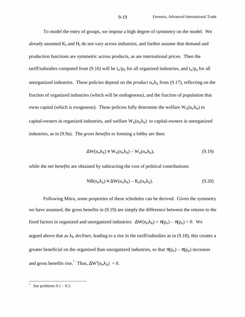
Feenstra, Advanced International Trade9-19
To model the entry of groups, we impose a high degree of symmetry on the model. We
already assumed Ki and Hi do not vary across industries, and further assume that demand and
production functions are symmetric across products, as are international prices. Then the
tariff/subsidies computed from (9.16) will be to/po for all organized industries, and tu/pu for all
unorganized industries. These policies depend on the product noλk from (9.17), reflecting on the
fraction of organized industries (which will be endogenous), and the fraction of population that
owns capital (which is exogenous). These policies fully determine the welfare Wo(noλk) to
capital-owners in organized industries, and welfare Wu(noλk) to capital-owners in unorganized
industries, as in (9.9a). The gross benefits to forming a lobby are then:
∆W(noλk) ≡ Wo(noλk) – Wu(noλk), (9.19)
while the net benefits are obtained by subtracting the cost of political contributions:
NB(noλk) ≡ ∆W(noλk) – Ro(noλk). (9.20)
Following Mitra, some properties of these schedules can be derived. Given the symmetry
we have assumed, the gross benefits in (9.19) are simply the difference between the returns to the
fixed factors in organized and unorganized industries: ∆W(noλk) = π(po) – π(pu) > 0. We
argued above that as λk declines, leading to a rise in the tariff/subsidies as in (9.18), this creates a
greater beneficial on the organized than unorganized industries, so that π(po) – π(pu) increases
and gross benefits rise.7 Thus, ∆W’(noλk) < 0.
7 See problems 9.1 – 9.3.
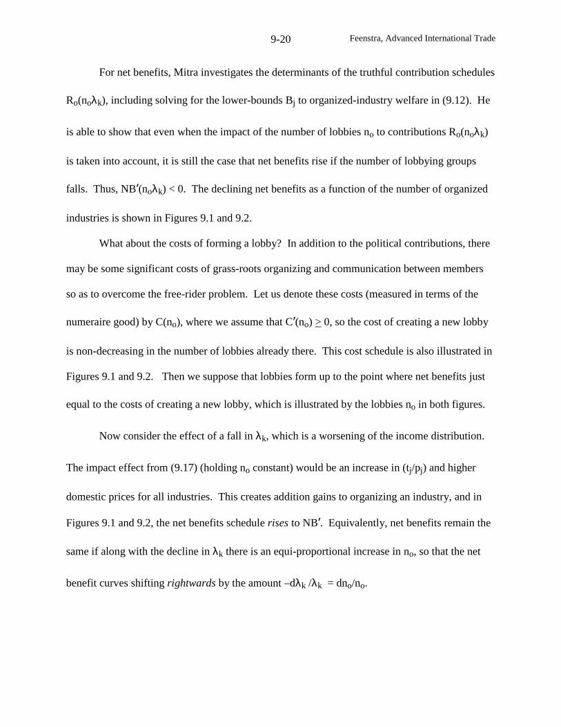
Feenstra, Advanced International Trade9-20
For net benefits, Mitra investigates the determinants of the truthful contribution schedules
Ro(noλk), including solving for the lower-bounds Bj to organized-industry welfare in (9.12). He
is able to show that even when the impact of the number of lobbies no to contributions Ro(noλk)
is taken into account, it is still the case that net benefits rise if the number of lobbying groups
falls. Thus, NB’(noλk) < 0. The declining net benefits as a function of the number of organized
industries is shown in Figures 9.1 and 9.2.
What about the costs of forming a lobby? In addition to the political contributions, there
may be some significant costs of grass-roots organizing and communication between members
so as to overcome the free-rider problem. Let us denote these costs (measured in terms of the
numeraire good) by C(no), where we assume that C’(no) > 0, so the cost of creating a new lobby
is non-decreasing in the number of lobbies already there. This cost schedule is also illustrated in
Figures 9.1 and 9.2. Then we suppose that lobbies form up to the point where net benefits just
equal to the costs of creating a new lobby, which is illustrated by the lobbies no in both figures.
Now consider the effect of a fall in λk, which is a worsening of the income distribution.
The impact effect from (9.17) (holding no constant) would be an increase in (tj/pj) and higher
domestic prices for all industries. This creates addition gains to organizing an industry, and in
Figures 9.1 and 9.2, the net benefits schedule rises to NB’. Equivalently, net benefits remain the
same if along with the decline in λk there is an equi-proportional increase in no, so that the net
benefit curves shifting rightwards by the amount –dλk /λk = dno/no.
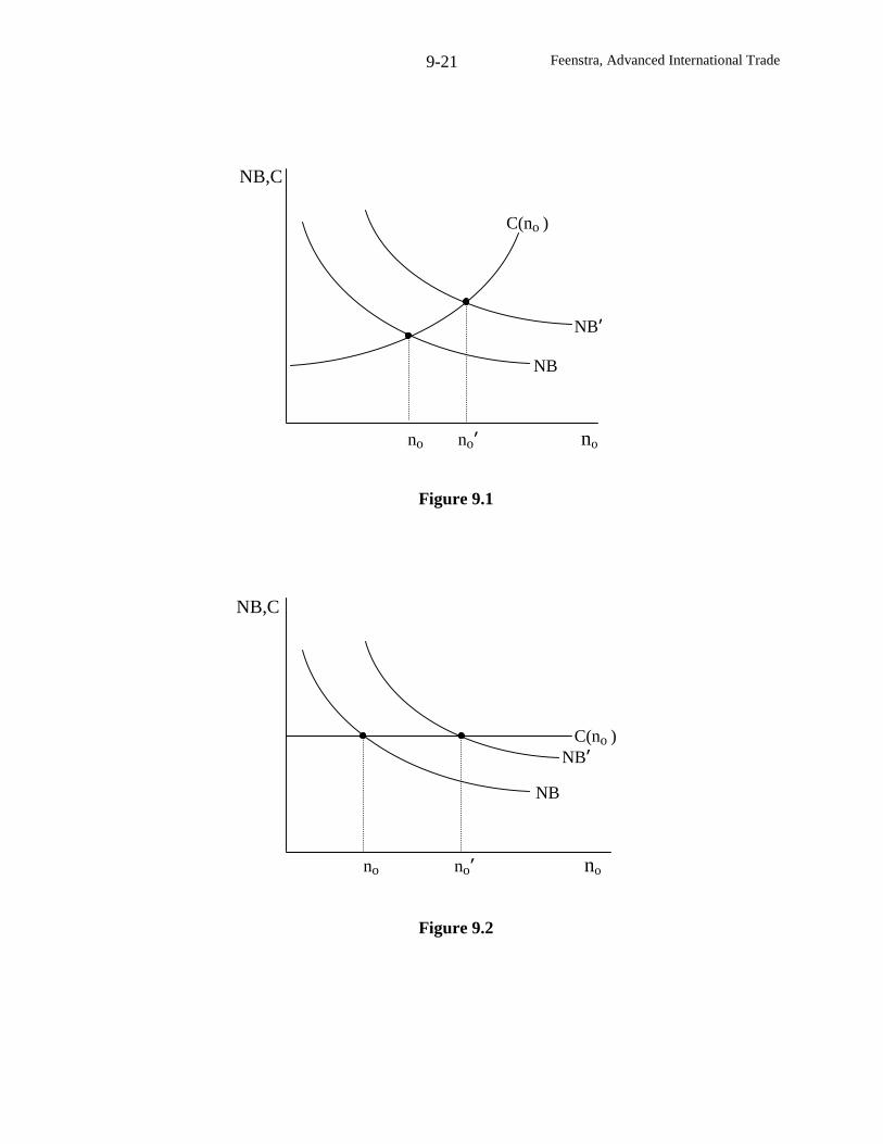
Feenstra, Advanced International Trade9-21
no no’ no
NB
NB,C
C(no )
Figure 9.1
NB’
NB
no no’ no
NB,C
C(no )
Figure 9.2
NB’
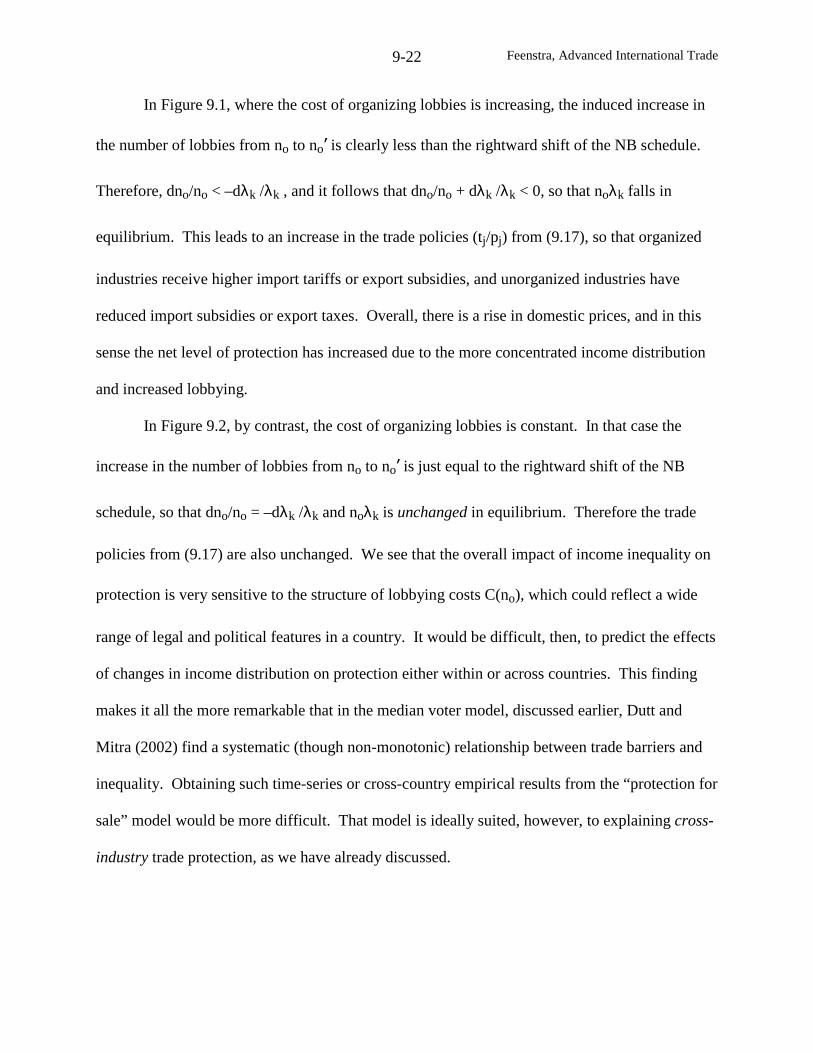
Feenstra, Advanced International Trade9-22
In Figure 9.1, where the cost of organizing lobbies is increasing, the induced increase in
the number of lobbies from no to no’ is clearly less than the rightward shift of the NB schedule.
Therefore, dno/no < –dλk /λk , and it follows that dno/no + dλk /λk < 0, so that noλk falls in
equilibrium. This leads to an increase in the trade policies (tj/pj) from (9.17), so that organized
industries receive higher import tariffs or export subsidies, and unorganized industries have
reduced import subsidies or export taxes. Overall, there is a rise in domestic prices, and in this
sense the net level of protection has increased due to the more concentrated income distribution
and increased lobbying.
In Figure 9.2, by contrast, the cost of organizing lobbies is constant. In that case the
increase in the number of lobbies from no to no’ is just equal to the rightward shift of the NB
schedule, so that dno/no = –dλk /λk and noλk is unchanged in equilibrium. Therefore the trade
policies from (9.17) are also unchanged. We see that the overall impact of income inequality on
protection is very sensitive to the structure of lobbying costs C(no), which could reflect a wide
range of legal and political features in a country. It would be difficult, then, to predict the effects
of changes in income distribution on protection either within or across countries. This finding
makes it all the more remarkable that in the median voter model, discussed earlier, Dutt and
Mitra (2002) find a systematic (though non-monotonic) relationship between trade barriers and
inequality. Obtaining such time-series or cross-country empirical results from the “protection for
sale” model would be more difficult. That model is ideally suited, however, to explaining cross-
industry trade protection, as we have already discussed.
Feenstra, Advanced International Trade9-23
Two-Country Model
In the median voter model and the “protection for sale” model of Grossman and Helpman
(1994), the governments treats the international price p* as fixed. But what if instead the country
is large, so that its tariffs affect the terms of trade? Obtaining a terms of trade gain creates an
additional reason to use tariffs. In a two-country model, both countries would have this
incentive, and we could conjecture that they would both end up with tariffs higher than those we
solved for above. Bagwell and Staiger (1999, 2002) argue that this creates an important role for
international institutions such as the GAT/WTO: to offset or eliminate the incentive to
manipulate the terms of trade.
To formalize this idea, we return to the median voter or the “protection for sale” model.
For simplicity, suppose that there are only two goods: the additively-separable numeraire good
that is exported from the home country, and a second good with demand d(p) at home and supply
y(p). Home imports are then m(p) = d(p) – y(p). Likewise, the foreign country has demand
d*(p*) for this good, and supply y*(p*), depending on its own price p*. Foreign exports are
denoted by x*(p*) = y*(p*) – d*(p*).
Home and foreign prices differ due to tariffs in both countries. Suppose that the home
country applies an ad valorem tariff, and let τ equal one plus the ad valorem tariff. Then the
home prices are p = pwτ, where p
ware the world prices. The foreign country applies an ad
valorem tariff on its own imports, and let τ* equal one plus the foreign ad valorem tariff. Since
pw
is the world relative price of the home import and foreign export, then 1/pw
is the world
relative price of the foreign import. Applying the tariff of τ* means that the foreign price of its
import good is τ*/pw
, so the relative price of the foreign export is pw
/τ*.
Feenstra, Advanced International Trade9-24
Using these prices, market clearing means that home imports equal foreign exports:
m(pwτ) = x*(p
w/τ*) ⇒ p
w(τ, τ*). (9.21)
This equation determines the world equilibrium price pw
(τ, τ*), depending the tariff in each
country. Under the standard assumptions on the import demand and export supply curves, it is
readily confirmed that:
τ<<
τ d
dp0
d
dpw
, and*d
*dp0
*d
dpw
τ>>
τ. (9.22)
In other words, the home tariff lowers the world price of imports for the home country and raises
the domestic price, while the foreign tariff raises the world price of its exports and lowers its
local price of the export good.8
Let us now consider the government objective function in each country. In the median
vote model the objective function was welfare of the median voter )I,p(V m , where from (9.2’)
income of the median voter was: ]T)p(py)p(yK)p(r)1[(I 0mm +++−ρ= .9 Using the ad
valorem tariffs defined above, tariff revenue in this expression is T = (τ – 1)pw
[d(p) – y(p)].
Because domestic prices are p = pwτ, we can substitute this into tariff revenue and income, and
obtain an expression for income that depends on the world price and domestic tariff, ),p(I wm τ .
It follows that the objective of the home government is:
G(pw
,τ) = )],p(I,p[V wmw ττ . (9.23)
8 You are asked to demonstrate (9.22) in problem 9.4.9 We now normalized the size of the population at L = 1 to simplify notation.
Feenstra, Advanced International Trade9-25
Thus, the objective function of the home government can be written as a function of the world
prices, and the tariff. Bagwell and Staiger argue that this formulation of the objective function is
general enough to encompass a number of models, including the median voter model and the
“protection for sale” model of Grossman and Helpman.10
Furthermore, it is readily verified that the tariffs in the median voter model (equation 9.4)
or in the “protection for sale” model (equation 9.15), satisfy the first-order condition:
Gτ(pw
, τ) = 0 . (9.24a)
That is, these tariffs are obtained by maximizing the government’s objective while treating the
world price pw
as fixed. For the foreign country there will be an analogous objective function
G*(pw
, τ*), with first-order condition for the tariff:
0*),p(G w* =ττ . (9.24b)
Bagwell and Staiger refer to the tariffs satisfying (9.24) as politically optimal.
However, the tariffs satisfying (9.24) will generally not be chosen by a government that
recognizes its ability to influence the terms of trade. Instead, the tariffs would be chosen in the
two countries to achieve:
0Gp
G]*),,(p[Gd
d w
pw =+
τ∂∂=τττ
τ τ , (9.25a)
and in the foreign country,
0G*
pG*]*),,(p[*G
d
d **
w*p
w =+τ∂
∂=ττττ τ . (9.25b)
10 Notice that G in (9.11) is a function of domestic prices p, but also depends on international prices p* which wedid not make explicit. Then G(p,p*) can be rewritten as G(τp*, p*), so that G again depends on p* and τ.
Feenstra, Advanced International Trade9-26
Notice the obvious difference between the politically optimal tariffs in (9.24), and the first-order
conditions (9.25) that incorporate the terms of trade effects. Bagwell and Staiger refer to the
tariffs satisfying (9.25) as the Nash equilibrium tariffs, since they are the best response by each
country given the tariff choice of the other.
The question then arises as to how the politically optimal tariffs (which ignore the terms
of trade effects) compare with the Nash equilibrium tariffs (which incorporate these effects). To
make this comparison, it is convenient to define the reduced form government objective
functions as,
]*),,(p[G*),(G~ w τττ≡ττ , (9.26a)
and in the foreign country,
*]*),,(p[*G*),(*G~ w τττ≡ττ . (9.26b)
These give the objectives as functions of the tariffs in the two countries. Notice that the
Nash equilibrium in (9.25a) can be equivalently written as 0G~ =τ , which defines the best home
response τ = r(τ*) to the foreign tariff. Similarly, the Nash equilibrium in (9.25b) can be written
as, 0G~ *
* =τ , which defines the best foreign response τ* = r*(τ) to the home tariff.
The Nash equilibrium is defined by the intersection of these reaction curves τ = r(τ*) and τ* =
r*(τ). Assuming that this intersection is unique, it is illustrated by point N in Figure 9.3. Since
this is the maximum of *),(G~ ττ subject to a given τ*, the iso-curve of *),(G
~ ττ will be concave
with slope infinity at point N, and is increasing in the leftward direction, as illustrated. Similarly,
the iso-curve of *),(*G~ ττ has a slope of zero at point N, and is increasing in the downward
direction, as illustrated. It is evident that there is a region below and to the left of point N,
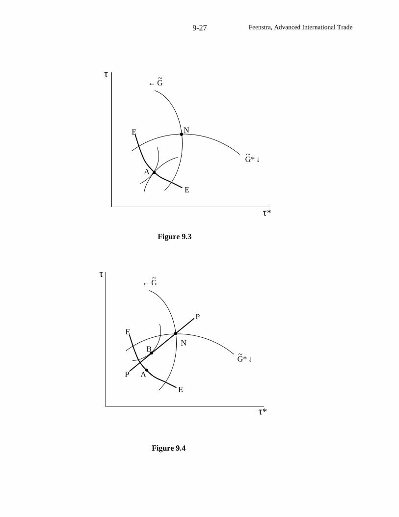
Feenstra, Advanced International Trade9-27
N
↓*G~
E
E
τ*
τG~←
A
↓*G~
E
E
τ*
τG~←
P
Figure 9.3
Figure 9.4
P
B
A
N
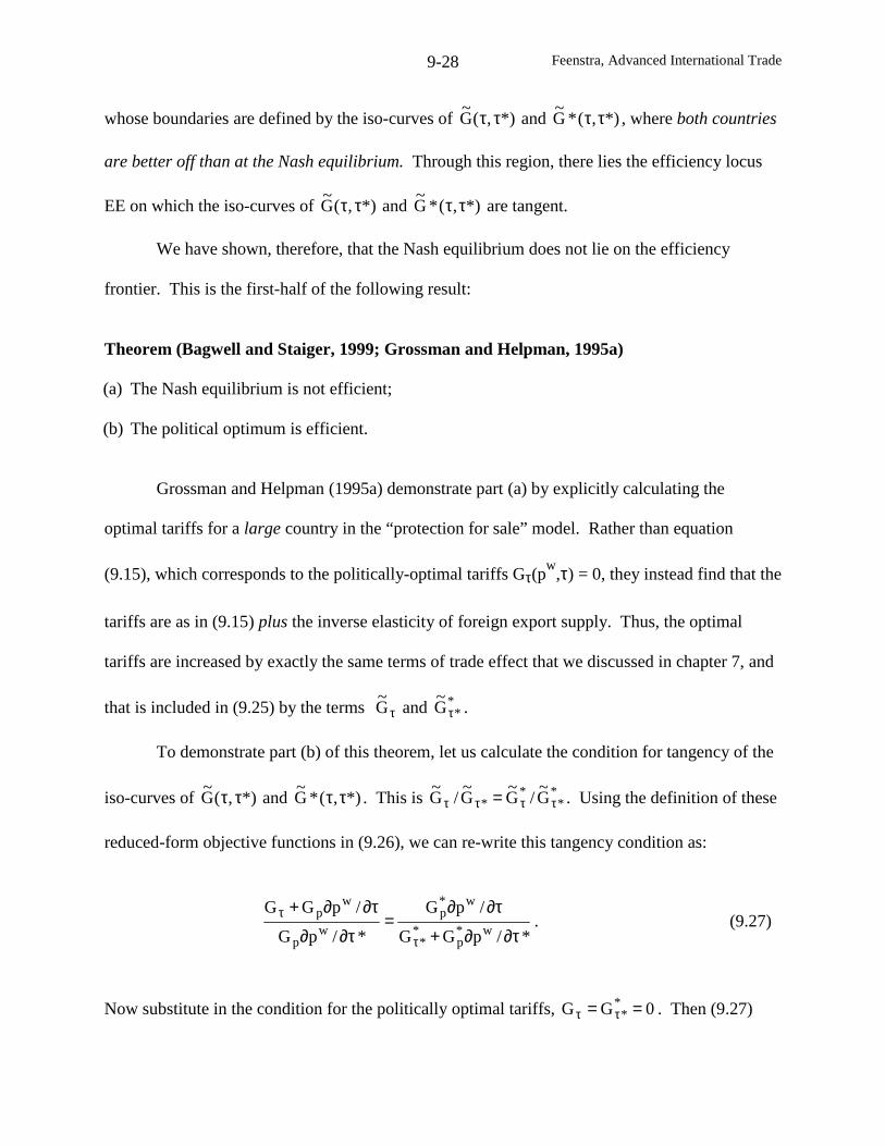
Feenstra, Advanced International Trade9-28
whose boundaries are defined by the iso-curves of *),(G~ ττ and *),(*G
~ ττ , where both countries
are better off than at the Nash equilibrium. Through this region, there lies the efficiency locus
EE on which the iso-curves of *),(G~ ττ and *),(*G
~ ττ are tangent.
We have shown, therefore, that the Nash equilibrium does not lie on the efficiency
frontier. This is the first-half of the following result:
Theorem (Bagwell and Staiger, 1999; Grossman and Helpman, 1995a)
(a) The Nash equilibrium is not efficient;
(b) The political optimum is efficient.
Grossman and Helpman (1995a) demonstrate part (a) by explicitly calculating the
optimal tariffs for a large country in the “protection for sale” model. Rather than equation
(9.15), which corresponds to the politically-optimal tariffs Gτ(pw
,τ) = 0, they instead find that the
tariffs are as in (9.15) plus the inverse elasticity of foreign export supply. Thus, the optimal
tariffs are increased by exactly the same terms of trade effect that we discussed in chapter 7, and
that is included in (9.25) by the terms τG~
and **G
~τ .
To demonstrate part (b) of this theorem, let us calculate the condition for tangency of the
iso-curves of *),(G~ ττ and *),(*G
~ ττ . This is **
** G
~/G
~G~
/G~
ττττ = . Using the definition of these
reduced-form objective functions in (9.26), we can re-write this tangency condition as:
*/pGG
/pG
*/pG
/pGGw*
p*
*
w*p
wp
wp
τ∂∂+
τ∂∂=
τ∂∂
τ∂∂+
τ
τ . (9.27)
Now substitute in the condition for the politically optimal tariffs, 0GG ** == ττ . Then (9.27)
Feenstra, Advanced International Trade9-29
simply becomes *)/p()/p(*)/p()/p( wwww τ∂∂τ∂∂=τ∂∂τ∂∂ , which is obviously satisfied.
Therefore, the political optimum lies on the efficiency locus, as illustrated by point A in Figure
9.3. It follows that the Nash equilibrium N is worse for both countries than the political
optimum at point A.11
This raises the question of whether it is possible to improve on the Nash equilibrium by
some simple rules agreed upon by both countries. Bagwell and Staiger (1999, 2002) argue that
this creates an important role for the GATT, and in particular, justifies the GATT principles of
reciprocity and nondiscrimination. As they describe (1999, pp. 216-217): “the principle of
reciprocity is a GATT norm under which one country agrees to reduce its level of protection in
return for a reciprocal ‘concession’ from its trading partner…The principle of nondiscrimination
is a separate norm, under which a member government agrees that any tariff on a given product
applies to the import of one trading partner applies equally to all other trading partners.” We will
examine the first of these principles.
How is reciprocity applied in practice? Bagwell and Staiger suggest the following
definition in our two-country model: the tariffs τ and τ* are reduced so that import levels in both
countries rise by the same amount. Since these imports occur in different goods, they must be
compared at some prices, so let us use the initial world prices pw0
. Then the tariff reductions are
reciprocal if pw0∆m = ∆m*, where m* is foreign imports of the numeraire good. But from trade
balance, the value of imports equals the value of exports abroad, so that ∆m* = m*1– m*
0=
pw1
x*1– p
w0x*
0. But we also know that foreign exports equal home imports, so that x*
1= m
1
11 We have not quite shown this last result, because it is possible that the countries are so asymmetric in size thatthe political optimum at point A lies on the efficiency locus EE, but outside the region bounded by the iso-curves ofG~ and *G
~ in Figure 9.1. We assume that this asymmetric case does not apply.
Feenstra, Advanced International Trade9-30
and x*0= m
0. Therefore, Bagwell and Staiger’s definition of reciprocity implies:
4444 34444 214444 34444 21importsForeign
00w11w
importsHome
00w10w0w mpmp*mmpmpmp∆∆
−=∆=−=∆ . (9.28)
By inspection, this equality is satisfied if and only if world prices are constant, pw1
= pw0
. So the
implication of reciprocity in the two-country model is that mutual tariff reductions should leave
the world price unchanged.
Totally differentiating the world price pw
(τ,τ*), it is unchanged when:
0*d*d
dpd
d
dp ww
=ττ
+ττ
⇒ 0d
dp
*d
dp
*d
d ww
>ττ
−=ττ
, (9.29)
where the positive sign follows from the inequalities in (9.22). The locus of tariffs along which
the world price pw
(τ,τ*) is held fixed at its Nash-equilibrium level is illustrated by PP in Figure
9.4. Since this line has a positive slope, and the iso-curves of *),(G~ ττ and *),(*G
~ ττ have
slopes of infinity and zero at point N, the PP locus clearly falls inside the region bounded by
those iso-curve. Therefore, reciprocal reductions in tariffs from the Nash equilibrium raise the
government objective function for both countries. This result provides strong justification for the
GATT principle of reciprocity.
How far should the tariff reductions proceed? Bagwell and Staiger argue that if the two
countries are symmetric in size, then the line PP will intersect the efficiency locus at precisely
the political optimum at point A. That is, tariff reduction should proceed until both countries are
applying tariffs as in the median voter or “protection for sale” model, and therefore avoiding the
mutual losses associated with exploiting the terms of trade.
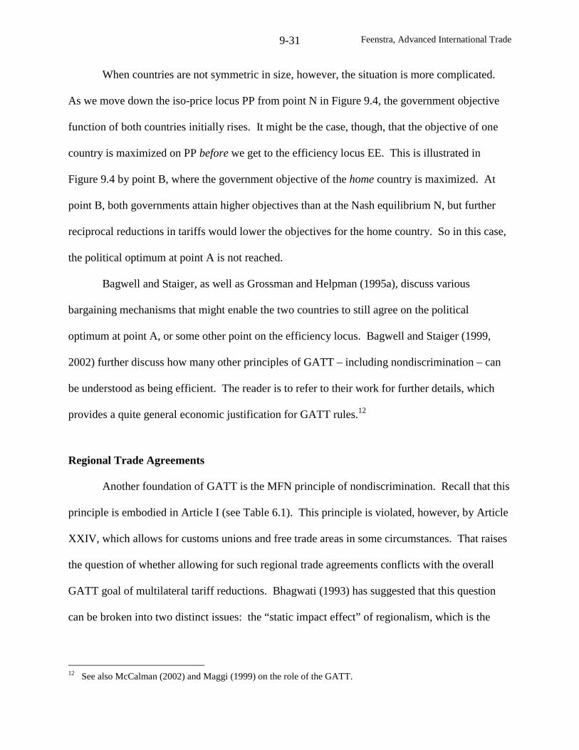
Feenstra, Advanced International Trade9-31
When countries are not symmetric in size, however, the situation is more complicated.
As we move down the iso-price locus PP from point N in Figure 9.4, the government objective
function of both countries initially rises. It might be the case, though, that the objective of one
country is maximized on PP before we get to the efficiency locus EE. This is illustrated in
Figure 9.4 by point B, where the government objective of the home country is maximized. At
point B, both governments attain higher objectives than at the Nash equilibrium N, but further
reciprocal reductions in tariffs would lower the objectives for the home country. So in this case,
the political optimum at point A is not reached.
Bagwell and Staiger, as well as Grossman and Helpman (1995a), discuss various
bargaining mechanisms that might enable the two countries to still agree on the political
optimum at point A, or some other point on the efficiency locus. Bagwell and Staiger (1999,
2002) further discuss how many other principles of GATT – including nondiscrimination – can
be understood as being efficient. The reader is to refer to their work for further details, which
provides a quite general economic justification for GATT rules.12
Regional Trade Agreements
Another foundation of GATT is the MFN principle of nondiscrimination. Recall that this
principle is embodied in Article I (see Table 6.1). This principle is violated, however, by Article
XXIV, which allows for customs unions and free trade areas in some circumstances. That raises
the question of whether allowing for such regional trade agreements conflicts with the overall
GATT goal of multilateral tariff reductions. Bhagwati (1993) has suggested that this question
can be broken into two distinct issues: the “static impact effect” of regionalism, which is the
12 See also McCalman (2002) and Maggi (1999) on the role of the GATT.
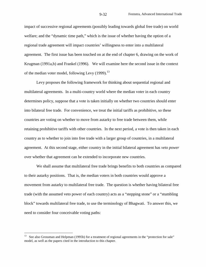
Feenstra, Advanced International Trade9-32
impact of successive regional agreements (possibly leading towards global free trade) on world
welfare; and the “dynamic time path,” which is the issue of whether having the option of a
regional trade agreement will impact countries’ willingness to enter into a multilateral
agreement. The first issue has been touched on at the end of chapter 6, drawing on the work of
Krugman (1991a,b) and Frankel (1996). We will examine here the second issue in the context
of the median voter model, following Levy (1999).13
Levy proposes the following framework for thinking about sequential regional and
multilateral agreements. In a multi-country world where the median voter in each country
determines policy, suppose that a vote is taken initially on whether two countries should enter
into bilateral free trade. For convenience, we treat the initial tariffs as prohibitive, so these
countries are voting on whether to move from autarky to free trade between them, while
retaining prohibitive tariffs with other countries. In the next period, a vote is then taken in each
country as to whether to join into free trade with a larger group of countries, in a multilateral
agreement. At this second stage, either country in the initial bilateral agreement has veto power
over whether that agreement can be extended to incorporate new countries.
We shall assume that multilateral free trade brings benefits to both countries as compared
to their autarky positions. That is, the median voters in both countries would approve a
movement from autarky to multilateral free trade. The question is whether having bilateral free
trade (with the assumed veto power of each country) acts as a “stepping stone” or a “stumbling
block” towards multilateral free trade, to use the terminology of Bhagwati. To answer this, we
need to consider four conceivable voting paths:
13 See also Grossman and Helpman (1995b) for a treatment of regional agreements in the “protection for sale”model, as well as the papers cited in the introduction to this chapter.

Feenstra, Advanced International Trade9-33
(1) The median voter in at least one country rejects the bilateral agreement, and then both
countries agree to the multilateral agreement;
(2) The median voters in both countries agree to the bilateral agreement and then agree to the
multilateral agreement;
(3) The median voters in both countries agree to the bilateral agreement and then both reject the
multilateral agreement;
(4) The median voters in both countries agree to the bilateral agreement, but then one country
vetoes the multilateral deal, whereas the other country would approve multilateral free trade.
Paths (1) and (2) are both possibilities, but in those cases the bilateral arrangement does
not act as a hindrance to multilateral free trade. The multilateral deal is rejected in paths (3) and
(4), so we need to examine whether these paths can actually occur. Case (4) can be ruled out by
the assumption that the time spent in bilateral free trade is very short as compared to the time
spent in multilateral free trade (if approved). This means that the median voter in the country
that benefits from bilateral free trade, and then also benefits from multilateral trade, will
anticipate that the other country will block the multilateral deal. Therefore, this median voter
will refuse to approve the bilateral arrangement initially, correctly anticipating that multilateral
free trade will still be achieved (since by assumption, this is better for both countries than
autarky). By this argument, path (4) never occurs.
We are left, then, with only having to consider whether or not path (3) can occur: is it
possible that the median voters in both countries are worse off going from bilateral to
multilateral free trade, whereas they are better off going from autarky to multilateral free trade?
We will demonstrate that this is impossible with a HO production structure. After showing this,
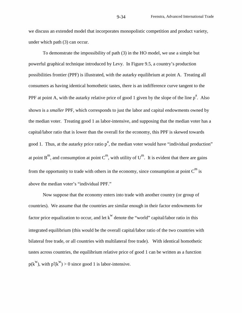
Feenstra, Advanced International Trade9-34
we discuss an extended model that incorporates monopolistic competition and product variety,
under which path (3) can occur.
To demonstrate the impossibility of path (3) in the HO model, we use a simple but
powerful graphical technique introduced by Levy. In Figure 9.5, a country’s production
possibilities frontier (PPF) is illustrated, with the autarky equilibrium at point A. Treating all
consumers as having identical homothetic tastes, there is an indifference curve tangent to the
PPF at point A, with the autarky relative price of good 1 given by the slope of the line pa. Also
shown is a smaller PPF, which corresponds to just the labor and capital endowments owned by
the median voter. Treating good 1 as labor-intensive, and supposing that the median voter has a
capital/labor ratio that is lower than the overall for the economy, this PPF is skewed towards
good 1. Thus, at the autarky price ratio pa, the median voter would have “individual production”
at point Bm
, and consumption at point Cm
, with utility of Um
. It is evident that there are gains
from the opportunity to trade with others in the economy, since consumption at point Cm
is
above the median voter’s “individual PPF.”
Now suppose that the economy enters into trade with another country (or group of
countries). We assume that the countries are similar enough in their factor endowments for
factor price equalization to occur, and let kw
denote the “world” capital/labor ratio in this
integrated equilibrium (this would be the overall capital/labor ratio of the two countries with
bilateral free trade, or all countries with multilateral free trade). With identical homothetic
tastes across countries, the equilibrium relative price of good 1 can be written as a function
p(kw
), with p’(kw) > 0 since good 1 is labor-intensive.
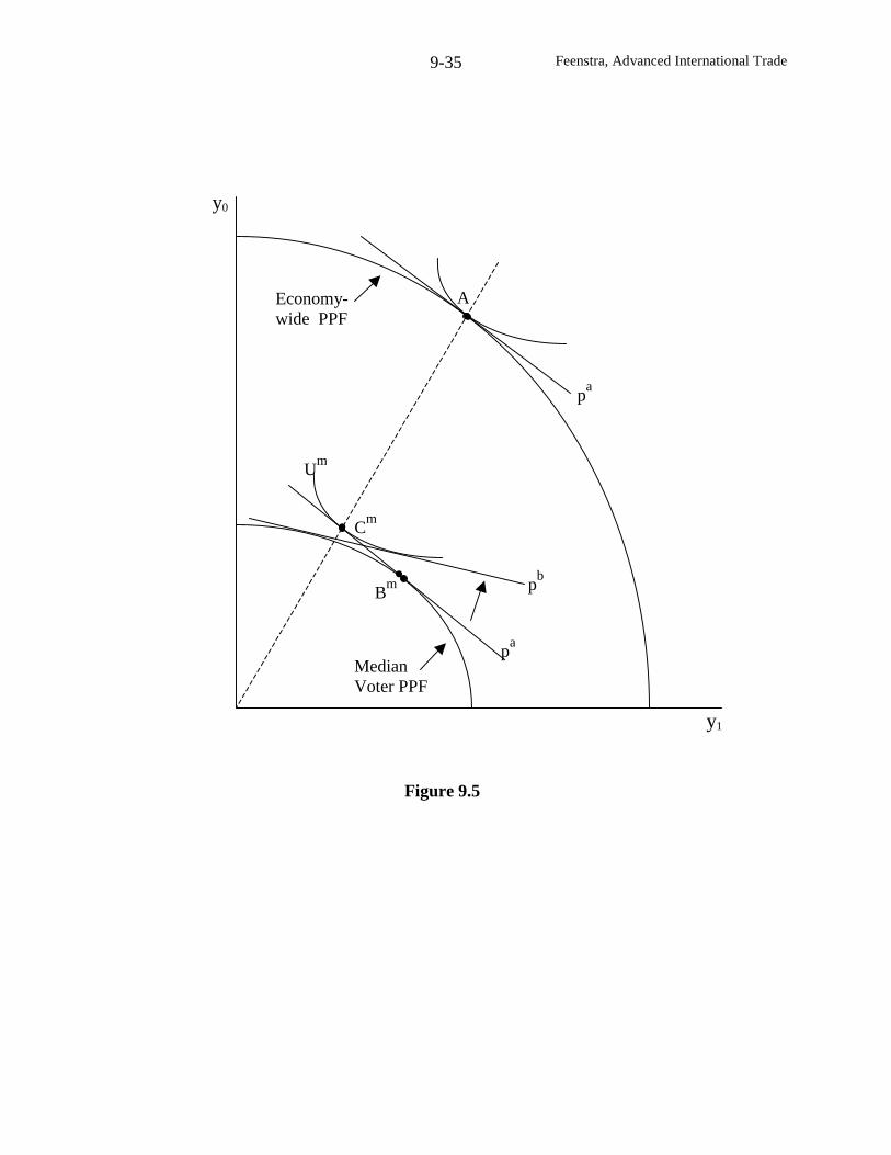
Feenstra, Advanced International Trade9-35
Cm
y0
Um
pa
y1
A
pa
Bm p
b
Figure 9.5
MedianVoter PPF
Economy-wide PPF
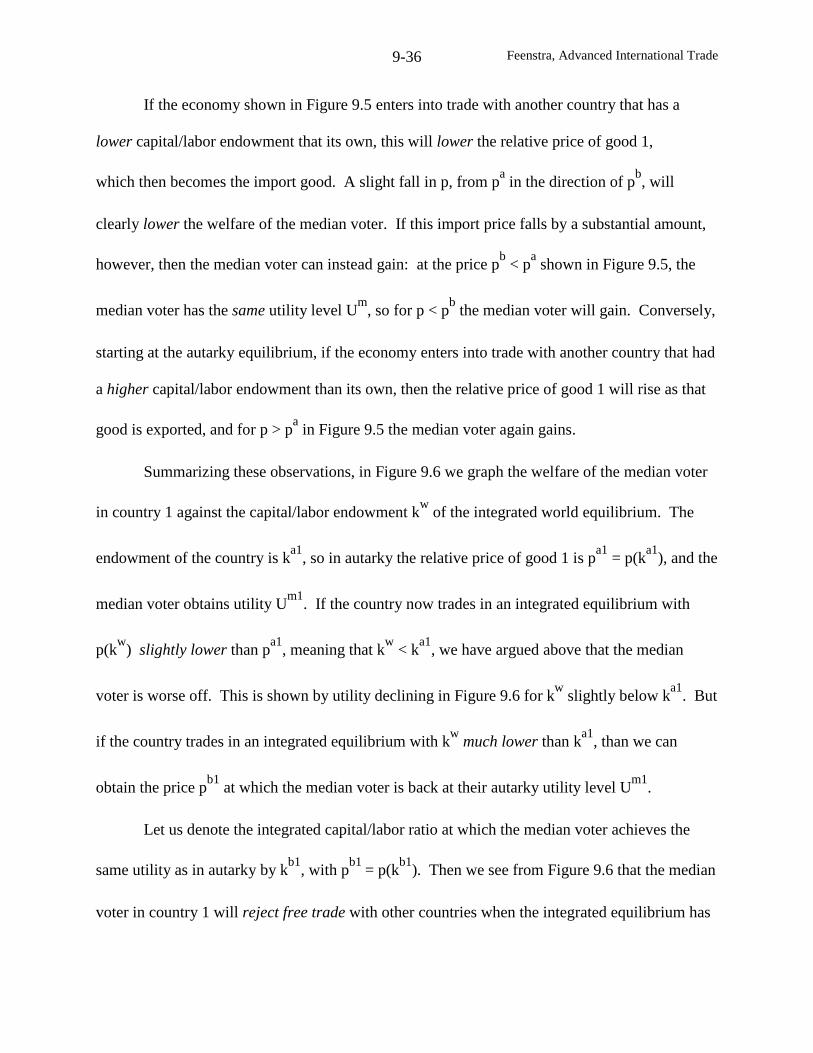
Feenstra, Advanced International Trade9-36
If the economy shown in Figure 9.5 enters into trade with another country that has a
lower capital/labor endowment that its own, this will lower the relative price of good 1,
which then becomes the import good. A slight fall in p, from pa
in the direction of pb, will
clearly lower the welfare of the median voter. If this import price falls by a substantial amount,
however, then the median voter can instead gain: at the price pb
< pa
shown in Figure 9.5, the
median voter has the same utility level Um
, so for p < pb
the median voter will gain. Conversely,
starting at the autarky equilibrium, if the economy enters into trade with another country that had
a higher capital/labor endowment than its own, then the relative price of good 1 will rise as that
good is exported, and for p > pa
in Figure 9.5 the median voter again gains.
Summarizing these observations, in Figure 9.6 we graph the welfare of the median voter
in country 1 against the capital/labor endowment kw
of the integrated world equilibrium. The
endowment of the country is ka1
, so in autarky the relative price of good 1 is pa1
= p(ka1
), and the
median voter obtains utility Um1
. If the country now trades in an integrated equilibrium with
p(kw
) slightly lower than pa1
, meaning that kw
< ka1
, we have argued above that the median
voter is worse off. This is shown by utility declining in Figure 9.6 for kw
slightly below ka1
. But
if the country trades in an integrated equilibrium with kw
much lower than ka1
, than we can
obtain the price pb1
at which the median voter is back at their autarky utility level Um1
.
Let us denote the integrated capital/labor ratio at which the median voter achieves the
same utility as in autarky by kb1
, with pb1
= p(kb1
). Then we see from Figure 9.6 that the median
voter in country 1 will reject free trade with other countries when the integrated equilibrium has
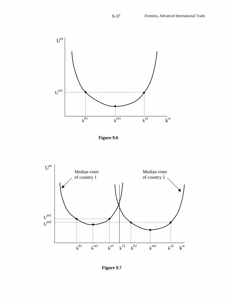
Feenstra, Advanced International Trade9-37
Um
kb1
km1
ka1 kw
Um1
Um
Um1
Um2
kb1
km1
ka1
k12
kb2
km2
ka2 kw
Figure 9.6
Figure 9.7
Median voterof country 1
Median voterof country 2
Feenstra, Advanced International Trade9-38
a capital/labor endowment kw ∈ (k
b1,k
a1), but otherwise will accept free trade for k
w ∉ (kb1
,ka1
).
Notice that the “rejection set” (kb1
, ka1
) is convex, which reflects the fact that utility of the
median voter, Um
(kw
), is a quasi-convex function of the capital/labor endowment in the
integrated equilibrium.
Now consider the situation of countries 1 and 2 deciding whether to engage in bilateral
free trade. In Figure 9.7 we graph the utilities of the median voters in each country. The
“rejection sets” are (kb1
, ka1
) and (kb2
, ka2
), and in the case we have illustrated country 2 is
capital-abundant, since its capital/labor endowment exceeds that of country 1, ka1
< ka2
. Then
with bilateral free trade, the integrated world equilibrium has a capital/labor endowment denoted
by k12
= (K1+K
2)/(L
1+L
2), and this lies in-between the capital/labor endowments of the two
countries, ka1
< k12
< ka2
. In order for the median voter in both countries to benefit from
bilateral free trade, it must be the case that k12
lies outside both the sets (kb1
, ka1
) and (kb2
, ka2
),
as illustrated. Since we also have that ka1
< k12
< ka2
, it then follows that bilateral free trade can
benefit both countries only if the two “rejection sets” are disjoint, as illustrated.
Now let us ask whether countries 1 and 2, which are both better off from bilateral free
trade, would be better or worse off from multilateral free trade. Let kw
denote the world
capital/labor endowment in that integrated equilibrium. If kw
= k12
then the two countries are
obviously indifferent between bilateral and multilateral free trade (since the relative price is not
affected). If kw
is slightly above k12
, then we can see from Figure 9.7 that country 1 would gain
moving from bilateral to multilateral, but country 2 would lose. On the other hand, if kw
is much
Feenstra, Advanced International Trade9-39
above k12
, so that kw
> ka2
in Figure 9.7, then it is possible that both countries gain. Checking
the other cases, if kw
is slightly below k12
, then country 2 would gain moving from bilateral to
multilateral, but country 1 would lose; while if kw
is much below k12
, so that kw
< kb1
, then it is
possible that both countries gain. In all cases, we see that countries 1 and 2 cannot both lose in
the move from bilateral to multilateral free trade. Therefore, we have proved part (a) of the
following:
Theorem (Levy, 1999)
(a) Under the 2x2 Heckscher-Ohlin production structure, if the median voters in both countries
gain from bilateral free trade, then at least one country must gain from multilateral free trade;
(b) Allowing for product variety under monopolistic competition, it is possible that the median
voters in both countries gain going from autarky to bilateral free trade, or from autarky to
multilateral free trade, but lose going from bilateral to multilateral free trade.
Part (a) this rules out path (3), and established that bilateral free trade agreement cannot
act as a hindrance to a multilateral deal. The essential logic is that the two countries will accept
the bilateral arrangement if only if their “rejection sets” are disjoint, with their combined
capital/labor endowment k12
lying in-between these sets. This immediately rules out having the
endowment kw
of a multilateral equilibrium contained in both sets. It is not difficult to see that
this logic extends to an initial free trade area involving any number of countries, who cannot
subsequently all lose from multilateral free trade.
Feenstra, Advanced International Trade9-40
Having established this result for the 2x2 HO model, what about more general models?
In part (b) of the theorem, we suppose that one sector produces a differentiated product under
monopolistic competition, while another sector produces a labor-intensive homogeneous good.
Furthermore, suppose that countries 1 and 2 are identical. There will still be gains from free
trade between them, just as was demonstrated in Krugman’s model at the beginning of chapter 5.
So the median voters in countries 1 and 2 both prefer the free trade area consisting of the country
pair (1, 2).
Now suppose that there is country 3, with the same production structure as 1 and 2 but
having a higher labor/capital endowment. Under multilateral free trade, it would produce more
of the labor-intensive homogeneous good, and for convenience suppose that it is fully specialized
in that good. Then the free trade area consisting of (1, 2) obtains no further product variety gains
from free trade with country 3, but there will still be a change in relative prices: since country 3
is labor-abundant, that would lower the relative price of that good. This can quite possibly lower
the welfare of the median voters in both countries 1 and 2. Therefore, it is entirely possible that
the median voters in countries 1 and 2 both lose going from bilateral to multilateral free trade.
Finally, we need to check whether our initial assumption – that country 1 and 2 are both
better off with multilateral free trade than in autarky – is satisfied in this example. That is, we
need to consider utility for the median voter in country 1 when it moves from autarky to free
trade with countries (2, 3) combined. Country 1 then gains from increased product variety with
the identical country 2, and possibly loses from the price change with labor-abundant country 3.
Provided that the product variety gains exceed the losses for the median voter due to import
competition, which is entirely possible, then country 1 gains overall from free trade with (2, 3).
The same argument applies to country 2 moving from autarky to free trade with (1, 3). So
Feenstra, Advanced International Trade9-41
despite the fact that multilateral free trade can bring gains as compared to autarky, we have
found that it can bring losses as compared to bilateral free trade. In this situation, the bilateral
agreement would prevent multilateral free trade from being pursued: it would indeed be a
stumbling block rather than a stepping stone. This demonstrates part (b) of the theorem, and the
general concern expressed by Bhagwati that regional trade agreements may inhibit the pursuit of
multilateral free trade.14
Political Economy of Foreign Investment in China
All of the applications in the chapter so far have been to economies governed by direct
democracy (with the median voter determining the optimal policy) or representative democracy
(where voters elect representatives who then determine policies). Grossman and Helpman
(2001) present a general formulation of democratic political systems where special interests exert
an influence on policies. We conclude this chapter with an application of their framework to a
non-democratic system – the People’s Republic of China. The motivation for this application is
much the same as in Goldberg and Maggi (1999): to use the observed levels of some policy
instrument or outcome to “reveal” the weights given by the government to various interest
groups. In the case of China, import tariffs have (until recently) been bound at relatively high
and inflexible levels, so that policy instrument cannot be used. Instead, we examine the policies
towards foreign investment, as indicated by the entry of foreign firms into various provinces, to
infer the weights in the government’s objective function.
The model we use relies on the choice of policies to influence foreign investment. We
shall not discuss the decisions of firms to enter foreign markets until the next chapter, but
14 McClaren (2002) further argues that introducing sector-specific sunk costs can have a similar effect, under whicha regional agreement can inhibit future multilateral deals.
Feenstra, Advanced International Trade9-42
introduce here the idea that they may enter a market to “jump the tariff,” i.e. because they cannot
export there due to tariff protection.15 Grossman and Helpman (1996) have introduced foreign
investment into their “protection for sale” model, and Branstetter and Feenstra (2002) make use
of that model to analyze policies towards multinationals in China, as follows.
Consumers are assumed to have preferences over an additively separable numeraire good
d0, and a CES aggregate denoted by D,
γ−γ
−γγ+= /)1(
0 D1
dU , γ > 0, γ ≠1, (9.30a)
where the CES aggregate is,
[ ] )1/(/)1(m
/)1(ff
/)1(hh Mdd)MN(dND
−σσσ−σσ−σσ−σ +−+= , σ > 1. (9.30b)
The values dj denotes consumption of the differentiated varieties from sources: j=h (home firms),
of which there are Nh in number; j=f (foreign imported products), of which there are (Nf – M);
and j=m (multinationals in China) of which there are M. As usual, σ is the elasticity of
substitution across individual varieties, while γ is the elasticity of demand for the aggregate good
D, and we add the restriction that σ > γ.
Branstetter and Feenstra (2002) suppose that the domestic industry is owned by the
government, as with state-owned firms in China. The profits earned by these firms receive extra
weight in the government’s objective function.16 The presence of multinationals presents a
15 Bhagwati (1996) has taken this argument a step further and suggested that foreign firms may enter a market to“defuse” the threat of future protection, in what he calls “quid-pro-quo” foreign investment. See also Bhagwati, et al(1987), Dinopoulos (1989, 1992), and Wong (1989).16 As Naughton (1996) and several other authors have noted, the Chinese government still relies on remittancesfrom state-owned enterprises for about two-thirds of its revenue.
Feenstra, Advanced International Trade9-43
potential threat to the state-owned enterprises through product market competition.17 This
creates a conflict between the entry of foreign firms and the profits of state-owned firms, that
must be resolved though government policy towards entry of the multinationals.
In designing the government policies, we allow the various provinces of China to
exercise autonomous control over multinational entry. This is broadly consistent with the
multiple layers of approval required for foreign investment in China. Only the largest projects
(initially $30 million but later $50 million) require approval from the central government,
whereas all projects require approval from the regional and provincial governments. In addition,
we suppose that the separate provinces control trade between themselves through internal border
barriers. The level of such barriers is the subject of current debate among experts on the Chinese
economy. On the one hand, Young (1997) has argued that internal border barriers are rising,
whereas Naughton (1999) disagrees. For reasons of modeling convenience, we take an extreme
version of the view in Young and assume there is no trade between the provinces. This means
that when a multinational enters one province, it is selling only to the local consumers. The
utility function in (9.30) therefore applies to each province, which differs in the number of firms
of each type found there.
We will suppose that labor is the only factor of production, and one unit of the numeraire
is produced with one unit of labor, so wages are unity. We shall assume, however, that the
multinational firms pay a wage premium of (w−1) > 0. The wage premium is meant to proxy for
a wide array of possible benefits that multinationals bring that are not captured in our model.
17 Notice that foreign investment might also be complementary rather than competitive, because until recently inChina the foreign firms were required to have local partners, which could benefit the state-owned enterprises. But anumber of studies suggest that the Chinese government, both national and local, is acutely aware of this competition,and has taken steps to impede the ability of foreign firms to compete in the Chinese market (e.g. Li and Chen, 1998;Rosen, 1999).
Feenstra, Advanced International Trade9-44
Costs for the locally produced products are cj, j = h, m. Costs for products produced abroad are
cf, but also face a specific tariff of t, so that marginal costs become cf + t. Prices are a standard
markup over these marginal costs, using the elasticity σ. We make the key assumption that cm <
cf + t. This assumption ensures that price charged by multinationals, pm, is less than that for
imports, pf. It follows that as more multinationals enter (M increases) and these products are
sold for pm < pf, the demand for products of the state-owned firms will decline due to
substitution away from these products. This is how product market competition between the
multinationals and domestic firms is captured in the model.
Each foreign firm faces the decision of whether to supply locally through imports, or
through setting up a local plant which requires a fixed cost of F > 0. We suppose that the
government also charges the multinational a profit tax of τ > 0. This instrument is supposed to
reflect the vast range of actual policies used in China to extract rents from multinationals, and
not just the corporate tax on multinationals.18 By modeling these policies as a tax on profits, we
are abstracting from the inefficiencies caused by actual policies.
The net profits earned locally are thus (1–τ)πm– F, where πm = pmdm/σ is profits under
the standard CES markup-pricing rule. Alternately, the multinational could just export to the
home country, and earn πf = pfdf/σ. Thus, entry will occur if and only (1–τ)πm– F > πf. This
condition is written as:
18 In fact, foreign firms are often taxed at zero or reduced rates for the first years of operation. Despite this, thereare many ways that local and national agencies extract rents from the multinationals. For example, the fact that mostmultinationals have had to use local partners reflects an implicit tax on their profits, which are shared with thepartner; similarly, the land-use fees that are commonly charged reduce the multinationals’ profits, as do conditionsof technology transfer and export requirements. Of course, bribes paid to allow multinationals to enter are another
Feenstra, Advanced International Trade9-45
σ≥−
στ− ffmm dp
Fdp
)1( . (9.31)
Entry is influenced through the profits tax τ and the specific tariff t, so the number of
multinational firms is written as a function M(τ,t). Multinationals react in the expected manner
to changes in these policies: when (9.31) holds as an equality, then τddM < 0 and dtdM > 0.
We now define the government’s objective function over the various interest groups,
beginning with consumer/worker utility U, which receives a weight of α. The profits of the
home state-owned firms are Nhπh = Nhphdh/σ, which accrue to the regional and national
government. We give revenue from state-owned firms a weight β in the objective function.
Finally, the government extracts rents Mτπmfrom the multinationals, and also collects tariff
revenue of (Nf − M)tdf . These two sources of revenue are each given weights of unity. The
objective function for each province is then defined by,
G(M,τ,t) ≡ αU + βNhπh + Mτπm + (Nf − M)tdf , (9.32)
where the multinationals entering each province are endogenously determined from (9.31).
We suppose that the central and the provincial governments jointly determine the rents
appropriated from the multinationals. The central government also chooses the tariff rate.
Denoting provinces by the subscript i, we let Gi[Mi(τi,t),τi,t] denote the objective function (9.32)
for each. Then the profit tax and tariff are chosen to solve:
example of the profit tax. Wei (1998) argues that corruption in China, which includes the need for “questionablepayments,” acts as a significant deterrent to foreign direct investment.
Feenstra, Advanced International Trade9-46
( )[ ]∑ τττ i
iiiii
t,,t,MGt,
max. (9.33)
We solve (9.33) over the choice of the profits tax rate τi, while a discussion of the
solution for tariffs t is in Branstetter and Feenstra (2002). Differentiating (9.33), the first-order
condition is that ∂Gi/∂Mi = –Miπmi /(∂Mi/∂τi). This means that the gain from attracting one more
multinational (∂Gi/∂Mi) is just balanced against the fall in the revenue τiMiπmi when the tax rate
is lowered to attract another multinational. That is, the regions are acting as monopsonists in
attracting foreign capital. This first-order condition for the choice of τi can be written as:19
ifiif
ifi
ffihi
i
i
i
ihimi s
MN
Ms
p
t)ss(
w
1w)1(
w
1wss ε+
−
+
σ−+
−−σα+
−η+β−= , (9.34)
where sj, j = h,f,m denotes the share of provincial consumption purchased from home state-
owned firms, imported products, or multinational products, respectively, and εi is a term
involving unobserved profit levels that is treated as a random error.
The first term on the right of (9.34) is the share of provincial consumption on state-owned
firms, which enters with the coefficient –β. Thus, the weight on state-owned firms in the
provincial objective function is simply obtained as the coefficient on their share in the regression
(9.34). A high weight on the state-owned firms indicates that in provinces where these firms are
more prevalent, the share of multinational firms will be correspondingly reduced. The next term
on the right of (9.34) is the wage premium paid by multinationals, which has the coefficient
19 This first-order condition is derived in Branstetter and Feenstra (2002).
Feenstra, Advanced International Trade9-47
η ≡ α(σ–1)(γ –1)/(σ –γ), which is of ambiguous sign. Following this is the wage premium times
the share of spending on state-owned firms plus imports. When the wage premium is higher, we
expect that regions would be more willing to accept multinationals, and this is confirmed by
having a positive coefficient α(σ–1) on that variable.
The estimate of σ itself comes from the next term, which is the tariff rate times the share
of spending on imports. This term reflects the loss in tariff revenue as multinationals enter and
the coefficient is –σ.20 Thus, combined with the former coefficient we can recover an estimate
of α. The final term reflects the number of multinationals times the share of imports. For
simplicity we measure the number of multinationals Mi by their capital stock in each province,
and treat the number of foreign firms wanting to export or invest in China, Nf, as constant over
provinces and time and estimate it as a coefficient.
For estimation, a time subscript is added to most variables in (9.33). There is an obvious
endogeneity problem in that the share of state-owned sales, on the right, will be correlated with
the share of multinational sales (since all the shares sum to unity), and to offset this, Branstetter
and Feenstra estimate (9.33) in levels rather than shares (i.e. multiplying all variables by
provincial apparent consumption) and also use instruments and weights.21
The results from estimating (9.33) using a panel of data for Chinese provinces over 1984-
1995, are shown in Table 9.1. Each of the three columns of results uses a different estimation
20 See our discussion of Brecher and Diaz Alejandro (1977) in problem 11.1 of chapter 11.21 The instruments are: provincial electricity production (used as an instrument for expenditure on state-ownedfirms); indexes of urban, state and overall wages (used as instruments for the wage premium); provincial GDP,population, average rural and urban income (used as instruments for apparent consumption); provincial processingimports (used as an instrument for ordinary imports); and various interactions between these terms. The weightedregressions use provincial GDP as a weight
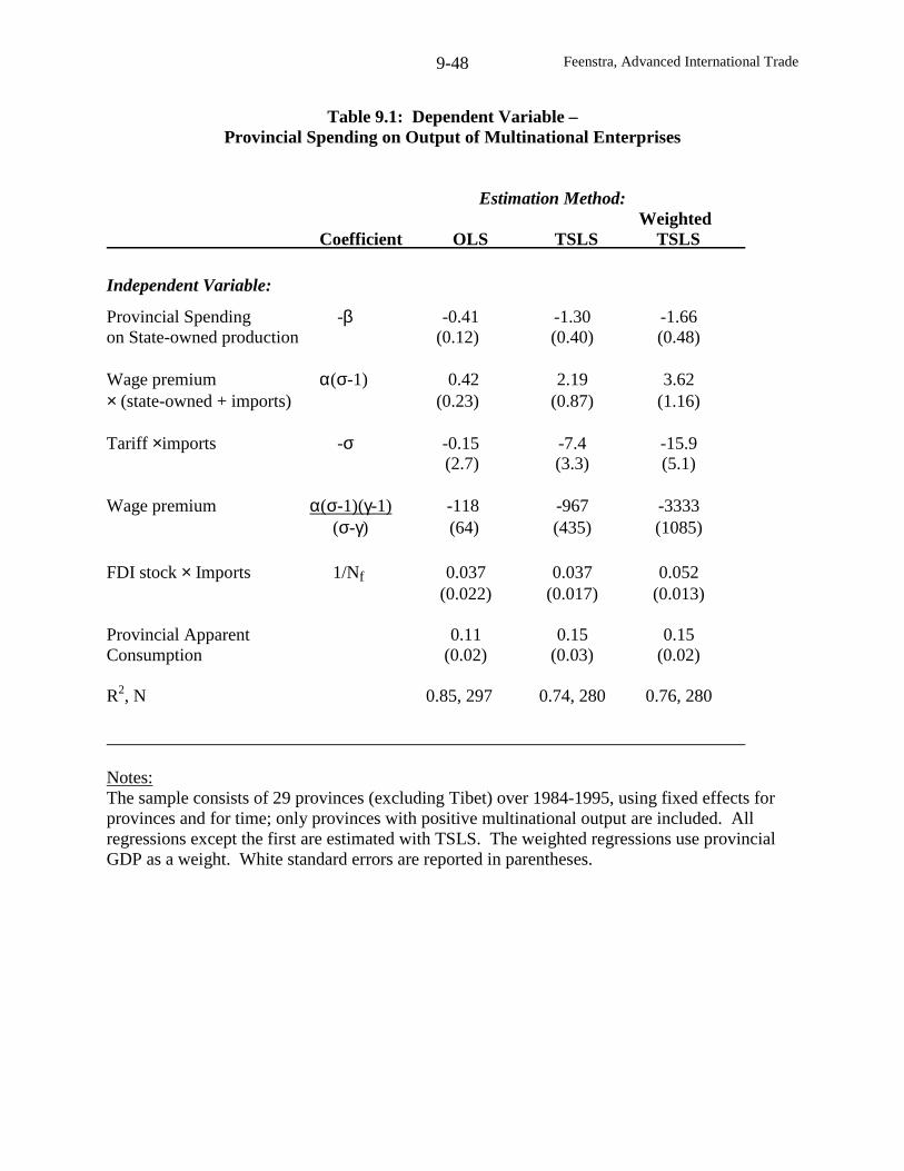
Feenstra, Advanced International Trade9-48
Table 9.1: Dependent Variable –Provincial Spending on Output of Multinational Enterprises
Estimation Method:Weighted
Coefficient OLS TSLS TSLS
Independent Variable:
Provincial Spending -β -0.41 -1.30 -1.66on State-owned production (0.12) (0.40) (0.48)
Wage premium α(σ-1) 0.42 2.19 3.62× (state-owned + imports) (0.23) (0.87) (1.16)
Tariff ×imports -σ -0.15 -7.4 -15.9(2.7) (3.3) (5.1)
Wage premium α(σ-1)(γ-1) -118 -967 -3333(σ-γ) (64) (435) (1085)
FDI stock × Imports 1/Nf 0.037 0.037 0.052(0.022) (0.017) (0.013)
Provincial Apparent 0.11 0.15 0.15Consumption (0.02) (0.03) (0.02)
R2, N 0.85, 297 0.74, 280 0.76, 280
Notes:The sample consists of 29 provinces (excluding Tibet) over 1984-1995, using fixed effects forprovinces and for time; only provinces with positive multinational output are included. Allregressions except the first are estimated with TSLS. The weighted regressions use provincialGDP as a weight. White standard errors are reported in parentheses.
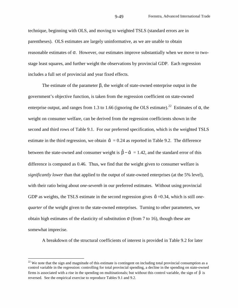
Feenstra, Advanced International Trade9-49
technique, beginning with OLS, and moving to weighted TSLS (standard errors are in
parentheses). OLS estimates are largely uninformative, as we are unable to obtain
reasonable estimates of σ. However, our estimates improve substantially when we move to two-
stage least squares, and further weight the observations by provincial GDP. Each regression
includes a full set of provincial and year fixed effects.
The estimate of the parameter β, the weight of state-owned enterprise output in the
government’s objective function, is taken from the regression coefficient on state-owned
enterprise output, and ranges from 1.3 to 1.66 (ignoring the OLS estimate).22 Estimates of α, the
weight on consumer welfare, can be derived from the regression coefficients shown in the
second and third rows of Table 9.1. For our preferred specification, which is the weighted TSLS
estimate in the third regression, we obtain α = 0.24 as reported in Table 9.2. The difference
between the state-owned and consumer weight is α−β ˆˆ = 1.42, and the standard error of this
difference is computed as 0.46. Thus, we find that the weight given to consumer welfare is
significantly lower than that applied to the output of state-owned enterprises (at the 5% level),
with their ratio being about one-seventh in our preferred estimates. Without using provincial
GDP as weights, the TSLS estimate in the second regression gives α =0.34, which is still one-
quarter of the weight given to the state-owned enterprises. Turning to other parameters, we
obtain high estimates of the elasticity of substitution σ (from 7 to 16), though these are
somewhat imprecise.
A breakdown of the structural coefficients of interest is provided in Table 9.2 for later
22 We note that the sign and magnitude of this estimate is contingent on including total provincial consumption as acontrol variable in the regression: controlling for total provincial spending, a decline in the spending on state-ownedfirms is associated with a rise in the spending on multinationals; but without this control variable, the sign of β isreversed. See the empirical exercise to reproduce Tables 9.1 and 9.2.
Feenstra, Advanced International Trade9-50
Table 9.2: Coefficient Estimates, by Time Period
Coefficient:α β σ
Sample:
1984-1995, 0.24 1.66 15.9(N=280) (0.07) (0.48) (5.1)
1988-1995, 0.24 1.32 11.5(N=210) (0.13) (0.50) (6.7)
1990-1995, 0.20 1.04 10.0(N=132) (0.15) (0.49) (7.6)
NotesComputed from the third regression reported in Table 9.1, but run over different samples.The estimation method is weighted TSLS. White standard errors are in parentheses.
Feenstra, Advanced International Trade9-51
sub-samples of the data, the 1988-1995 period and the 1990-1995 period. As we confine our
view to the later sub-samples, we lose observations and consequently precision in some of our
estimates; sub-periods smaller than 1990-1995 do not yield many significant coefficients at all.
In the later sub-periods, the estimated magnitude of the weight on state-owned enterprises falls.
This is consistent with the historical trend towards liberalization, of course. In the relatively
liberal 1990-95 sub-period, for example, we find that the weight on state-owned enterprises is
unity, which is still considerably higher than the weight on consumer welfare (though the
difference between them is no longer significantly different from zero).
These estimates provide a start contrast to the results of Goldberg and Maggi (1997) for
the U.S., where consumer welfare had a weight that was 50 to 100 times more than campaign
contributions. For China, we find that state-owned enterprises have a weight that is between four
and seven times greater than that given to consumers. The evidence of a political premium on
state-owned industries diminishes over time, but the point estimates still indicate these firms are
favored. Branstetter and Feenstra (2002) further investigate the impact on provincial objective
functions of the changes in tariff structure that China has promised under WTO accession. They
find that these changes could potentially lower welfare in some provinces, due to the exit of
multinationals. This provides some quantitative backing for skepticism that China, given the
current political equilibrium, will actually follow through with the promised liberalization in all
sectors and regions under its entry into the WTO.
Conclusions
In this chapter we have relied on two major models: the median voter model (first
applied to trade policy by Mayer, 1984), and “protection for sale” of Grossman and Helpman
(1994, 1995a,b, 1996). There are many other models of the political economy of trade policy,
Feenstra, Advanced International Trade9-52
and the reader is referred to Hillman (1989) and Rodrik (1995) for surveys. The median voter
model relies on a voting mechanism under direct democracy, and despite this rather simplified
framework, receives surprising empirical support from Dutt and Mitra (2002). In comparison,
the “protection for sale” model allows for the government to be influenced by many industry
lobbies. This has received strong empirical support for the U.S. from Goldberg and Maggi
(1999) and Gawande and Bandyopadhyay (2000), along with numerous empirical applications to
other countries, as surveyed by Gawande and Krishna (2003).
In their original formulations, the median voter and “protection for sale” models both
treat international prices as fixed, so that tariffs shift income between interest groups, but cannot
raise the welfare of all groups. In contrast, Bagwell and Staiger (1999, 2002) explicitly introduce
a large-country model, under which tariffs can improve the terms of trade and raise a country’s
welfare. The government objective function used by them encompasses the median voter and
“protection for sale” model, while Grossman and Helpman (1995a) also investigate terms of
trade effects in the latter model. A country that uses an import tariff to improve its terms of trade
does so at the expense of the other country (plus an added deadweight loss), so from the
viewpoint of world efficiency, it would be better for countries to agree to avoid such actions.
This creates an important role for the GATT, and the principle of reciprocity in tariff reductions
provides a way to eliminate the incentive to manipulate the terms of trade. Notice that even
under this principle, tariffs are still used in Bagwell and Staiger (1999, 2002) and Grossman and
Helpman (1995a) for political economy reasons.
We have also reviewed the role of regional trade agreements, and whether they help or
hinder the movement towards multilateral free trade. Levy (1999) employs a median voter
model to address this, while Grossman and Helpman (1995b) extend the “protection for sale”
Feenstra, Advanced International Trade9-53
model in that direction. Empirically, it would be difficult to infer the impact of regional
agreements on the pursuit of multilateral free trade, since the multilateral agreements of GATT
are themselves so infrequent. But there are a number of related empirical questions that can be
addressed. Krishna (2002) provides empirical evidence on the distance between countries and
the potential welfare gains from regional agreements. He finds that close trading partners do not
appear to have a “natural” advantage in created welfare-improving free trade areas. Baier and
Bergstrand (2002) and Magee (2002) introduce the endogeneity of free trade agreements into a
gravity equation, of the type discussed in chapter 5. These authors find that the impact of FTAs
is significantly affected by treating these agreements as endogenous. The variables they include
to explain free trade areas also provide a test of the determinants of these regions, and these
papers are recommended for further reading.
Feenstra, Advanced International Trade9-54
Problems
In the model of Mitra (1999), organized and unorganized industries are treated as
symmetric, having the same world prices, capital stocks, production and demand functions and
differ only in their lobbying ability. Therefore, the return to the fixed factor in any industry can
be written as π(pi) instead of πi(pi), depending on the price by not on any other industry
characteristic. Normalizing the world prices at unity, denote the price in organized industries by
po = 1 + to, and in unorganized industries by pu = 1 + tu. The following questions derive
additional results for that model:
9.1 Consider the return to the specific-factor in sector i, from (9.8):
]L)K,L(fp[)p( iiiL
maxi
i−=π ,
where we assume that fLL < 0. By differentiating the first-order condition for this problem and
using )p(y)p( ii =π′ , show that profits are a convex function of the industry price.
9.2 Replace λk no with λo in (9.17), and rewrite the optimal tariff to>0 and subsidy tu< 0 as,
,p
m)p(yt
1
jj
o
ojj
−
∂∂
λ+αλ−δ
= where δo = 1 and δu = 0.
Output depends on the industry price, but for convenience, we treat the import derivative as fixed
and equal across industries. Then computeo
o
d
dt
λand
o
u
d
dt
λ, and show that
o
o
d
dt
λ>
o
u
d
dt
λ.
Feenstra, Advanced International Trade9-55
9.3 Continuing to denote λk no by λo, consider the return to the specific factor in an organized
rather than an unorganized industry, ∆W(λo) = π(po) – π(pu). Using the results from problems
9.1 and 9.2, show that ∆W’(λo) = π’(po)(dto/dλo) – π’(pu)(dtu/dλo) < 0.
9.4 The equilibrium prices pw
(τ,τ*) in (9.21) are defined by m(pwτ) = x*(p
w/τ*). Assuming
that m’(pwτ) < 0 and x*’(pw/τ*) > 0, show that the inequalities in (9.22) hold.
Feenstra, Advanced International Trade9-56
Empirical Exercise
This exercise is to reproduce regression results Branstetter and Feenstra (2002). To complete the
exercise, the file “china_fdi.dta” should be stored in: c:\Empirical_Exercise\Chapter_9\.
Then do:
8.1 Run the program “share_reg.do” to reproduce the regression results in Table 9.1. Notice that
apparent consumption (“appcon3”) is included as a control variables in these regressions. What
happens if this variable is dropped?
8.2 Open the excel file “standard_errors.xls” to see how the results in Table 9.2 are computed.
What formula is used for α, and for its variance and standard error? Justify these formulas.
Hint: Consider the easier case of taking the difference between α and β. Then:
var(α – β) = E[(α – β) – )( β−α ]2
= E f(α,β),
where f(α,β) is the quadratic function indicated. To compute this expected value, we take a
second-order Taylor series expansion:
).)()(,(f))(,(f))(,(f
))(,(f))(,(f),(f),(f
2212
21 β−βα−αβα+β−ββα+α−αβα+
β−ββα+α−αβα+βα≈βα
αβββαα
βα
It follows that,
).,cov(),(f),(f),(f),(Ef 2212
21 βαβα+σβα+σβα≈βα αββββααα
So computing the derivatives of the quadratic function f(α,β), we obtain,
var(α – β) = E[(α – β) – )( β−α ]2
).,cov(222 βα−σ+σ≈ βα
Now given the formula for α, use the same approach to justify its variance.
Feenstra, Advanced International Trade
Chapter 10: Trade and Endogenous Growth
The link between trade and growth has long been a question of interest from both a
theoretical and policy point of view. David Ricardo developed a dynamic model of corn and
velvet production, with corn produced by land and labor and velvet produced with labor alone.1
The need to pay labor from a “wage fund” established prior to production prevents all labor from
being employed initially (i.e. there is a liquidity constraint on firms). Ricardo showed that in
autarky the gradual expansion of the wage fund and growth of velvet production would lower its
relative price, until a long-run equilibrium was reached. Opening trade, however, would allow
the relative price of velvet to be maintained at world levels, thereby benefiting capitalists at the
expense of landowners. This remarkable model has many of the issues that are of interest in
modern discussions of trade and growth: the possibility that growth will be associated with
continual changes in prices, and conversely, the impact of trade on prices and growth rates
themselves.
In the first of these issues we will be primarily concerned with the effects of growth on
the terms of trade, i.e. the price of exports relative to imports. This brings us to the famous case
of “immiserizing growth,” due to Bhagwati (1958), where we ask whether growth can actually
lower a country’s welfare due to a fall in the terms of trade. The idea that developing countries
might be subject to a decline in their terms of trade, particularly for primary commodities, is
associated with the Latin American economist Raul Prebisch (1950). While there is little
evidence to support that hypothesis in general, it is still the case that terms of trade decline due to
growth have been observed (Acemoglu and Ventura, 2002, Debaere, 2001).
1 See Findlay (1984, pp. 187-191), who cites this model to Ricardo’s Essay on the Influence of a Low Price of Cornupon the Profits of Stock (in Volume IV, pp. 1-42, of Ricardo, 1951).

Feenstra, Advanced International Trade10-2
In the second part of the chapter, we model the underlying determinants of growth
through research and development. This class of models goes by the name “endogenous
growth,” and their application to trade has been most thoroughly studied by Grossman and
Helpman (1991). We will describe just one of the models described by those authors, which is a
dynamic version of the CES monopolistic competition model presented in chapter 5.2 Even in
this case, we will find that trade can have a fairly wide range of results on product innovation
within a country and therefore on growth. When there is free trade in all goods, including free
international flows of knowledge, then trade raises growth rates and brings gains to all countries,
but this is not necessarily the case when there is free trade in only a subset of the goods without
flows of knowledge. Empirically, then, the beneficial effect of trade on growth depend very
strongly on whether there are international spillovers of knowledge, so we shall review the
empirical evidence on that and other topics.
We begin with a discussion of how to measure productivity growth. This is quite easy in
the case of perfect competition, but not under imperfect competition. In the latter case, it turns
out that conventional measures of productivity growth are biased due to increasing returns to
scale and the markup of price over marginal cost. Hall (1988) has proposed a method to correct
for this, and at the same time, estimate the markups. In the context of trade reform it allows us to
estimate the extent to which trade liberalization has led to a reduction in markups by firms facing
import competition. This approach has been applied to Turkey by Levinsohn (1993) and to the
Ivory Coast by Harrison (1994), as we shall discuss.
2 This model was introduced by Judd (1985), Grossman and Helpman (1989, 1990) and Romer (1990), and alsoapplied to trade by Rivera-Batiz and Romer (1991a,b). The alternative to the CES model is the “quality ladders”model of product improvement, as described by Segerstrom, et al (1990), Grossman and Helpman (1991) and Taylor(1993). There are many other writings on endogenous growth and trade, including Taylor (1994) on the gains fromtrade and Dinopoulos and Segerstrom (1999a,b) on the dynamic effects of tariffs.
Feenstra, Advanced International Trade10-3
Measurement of Productivity
Growth in the output of a firm or industry can occur due to growth in inputs (labor,
capital, and human capital), or due to an increase in output that is not explained by inputs: the
latter is called productivity growth. Specifically, suppose that output yi is produced using labor
Li and capital Ki, with the production function yi=Aif(Li,Ki), where Ai is a measure of Hick’s
neutral technological progress. Totally differentiating this, we have += )K,L(fdAdy iiii
iiKiiiLi dKfAdLfA + . Dividing this by yi = Aif(Li,Ki), and letting z/dzz = denote the
percentage change in any variable, we see that,
+
+= i
ii
iiKi
ii
iiLii K
)K,L(f
KfL
)K,L(f
LfAy . (10.1)
In general, then, productivity growth can be measured by the growth in output minus a
weighted average of the growth in inputs, where the weights are the elasticities of output with
respect to each factor. The difficulty is that these weights are not directly observable. With the
added assumption of perfect competition, however, the marginal products equal iiLi p/wfA =
and iiKi p/rfA = , so in that case the elasticities appearing in (10.1) are measured by θiL =
iii yp/wL and iiiiK yp/rK=θ , which are the revenue shares of labor and capital. Under the
further assumption of constant returns to scale, these shares sum to unity so that θiK = 1 – θiL.
Then we see from (10.1) that technological progress iA can be measured by the difference
between the growth of output and a share-weighted average of the growth in inputs, which is the
Feenstra, Advanced International Trade10-4
definition of total factor productivity (TFP) due to Solow (1957):3
]K)1(L[yTFP iiLiiLii θ−+θ−≡ . (10.1’)
Notice that this measure of productivity growth is indeed a “residual” – the portion of output
growth that is not explained by inputs – or a “measure of our ignorance,” in the memorable
phrase of Robert Solow.
Let us now weaken our assumptions, and allow for imperfect competition and increasing
returns to scale. To introduce increasing returns to scale, we assume that the production
function is homogeneous of degree µi > 1, so it follows that µif(Li,Ki) = (fiLLi + fiKKi).4
Substituting this into (10.1), we obtain,
+
+
+
µ+= iiiKiiL
iiKi
iiKiiL
iiLiii K
KfLf
KfL
KfLf
LfAy .
+
−+
+
µ+= iiiKiiL
iiLi
iiKiiL
iiLii K
KfLf
Lf1L
KfLf
LfA
iiiiii
iiLi K)KL(
)K,L(f
LfA µ+−
+= , (10.2)
where the last line follows from µif(Li,Ki) = (fiLLi + fiKKi) and simple arithmetic.
With imperfect competition in the product market, the equilibrium condition for the
3 In practice, total factor productivity in (10.1’) would be measured using first-differences rather than infinitesimal
changes, as ]iKln)iL1(iLlniL[iylniTFP ∆θ−+∆θ−∆≡ . We have already seen this definition of TFP in our
discussion of chapter 4, as well as the dual definition, ipln)irlniKiwlniL(iTFP ∆−∆θ−∆θ≡ , where wi is the wage, ri
is the rental on capital, and pi is the price in industry i. Note that with the log change in input quantities or prices
measured between two points in time, the factor cost-shares θij should be measured as the average between thesetwo periods; this method is called the Tornqvist index of total factor productivity (see Appendix A).
Feenstra, Advanced International Trade10-5
hiring of labor is,
wfA1
1p iLii
i =
η
− . (10.3)
where ηi is the (positive) elasticity of demand. It follows that the real wage equals
iLiiii fA]/)1[()p/w( η−η= . The share of labor in total revenue is then,
ii
iiL yp
wL=θ =
ii
iiLii
y
LfA)1(
η−η
=
η−η
)K,L(f
Lf1
ii
iiL
i
i , (10.4)
where the final equality follows from yi = Aif(Li,Ki). Thus, the labor share understates the
elasticity of output with respect to labor, since .1/)1( ii <η−η
Substituting (10.4) into (10.2), we see that output growth is related to true productivity
change by,5
iiiiiLiiii K)KL()]1/([Ay µ+−θ−ηη+= . (10.5)
Thus, we see that output growth is composed of true productivity change iA , plus the change in
labor/capital growth times the coefficient )1/( ii −ηη , plus capital growth times the returns to
scale parameters µi . The coefficient )1/( ii −ηη equals the ratio of price to marginal cost, so any
change in this coefficient are interpreted as evidence of changes in the price-cost markup.
Running (10.5) as a regression therefore allows us to measure the impact of trade liberalization
on the markups charged, as well as estimate the returns to scale.
4 See problem 1.2 in chapter 1.5 Alternatively, we can express (10.5) in first-differences and deduct ]iKln)iL1(iLlniL[ ∆θ−+∆θ from both
sides, obtaining iii Kln)1()iKlniLln(iL)]1/(1[iAlniTFP ∆−µ+∆−∆θ−η+∆= , using the definition of TFP from
note 4.
Feenstra, Advanced International Trade10-6
Harrison (1994) applies this technique to firm-level data for the Ivory Coast, which had
an import liberalization beginning in 1985. The estimating equation is (10.5) but written with
discrete rather than infinitesimal changes:
itititiLtitit Kln)KlnLln(Alnyln ∆µ+∆−∆θβ+∆=∆
ititititiLti Kln)KlnLln( ε+∆µ+∆−∆θβ+α= , (10.5’)
where in the second line we replace the true productivity change itAln∆ by αi + εit, composed
of a firm fixed-effect αi and a random component εit. The estimated ratio of price to marginal
cost, βt ≡ ηt/(ηt – 1), is treated as common across firms i = 1,…,N within each industry but is
allowed to change in the pre- and post-liberalization sample. Thus, by examining the change in
βt we can determine the effect of liberalization on markups.
Estimation is performed with both OLS and instrumental variables.6 Initial estimates
generally provided only insignificant changes in the estimated price-cost ratios. So rather than
just letting the markups βt change over time, Harrison instead interacts this variable with
industry-level estimates of import penetration. Specifically, let βt = β0 + β1Mt, where Mt is the
ratio of imports to consumption in each industry. Substituting this in (10.5’), we obtain an
interaction term between Mt and )KlnLln( ititiL ∆−∆θ , with the coefficient β1. We expect that
β1 < 0, so that higher imports lead to lower markups. Harrison obtains an estimate of –0.25 for
6 The error εit in (10.5’) is likely correlated with factor inputs on the right: a firm that experiences a boost toproductivity will hire more inputs. Appropriate instruments should be correlated with factor usage by the firm, butnot with productivity, and Harrison uses the nominal exchange rate, the price of energy, sectoral real wages, and thefirms’ reported debt. The endogeneity of inputs, and appropriate methods to correct for this, is also addressed byHall (1988), Olley and Pakes (1996) and Levinsohn and Petrin (2001).
Feenstra, Advanced International Trade10-7
β1 over the entire sample (standard error of 0.05). This indicates, for example, that an increase
in import penetration from 0 to 50% would reduce the ratio of price to marginal cost by 12%.
She also finds that reduced tariffs are associated with lower price-cost ratios, but that result is
only significant at the 15% level. So the connection between import liberalization and reduced
markups is weakly confirmed in her study.
Notice that in our derivation of (10.5) we did not assume that the rental on capital is
observable, but only used the labor share. If instead the rental is observable, then the capital
share is θiK = rKi/piyi = [(ηi – 1)/ηi][fiKKi/f(Li,Ki)], analogous to (10.4). Substituting these two
equations into (10.1), we obtain an alternative relationship between output growth and true
productivity change,7
( )iiKiiLi
iii KL
1Ay θ+θ
−η
η+= . (10.6)
Levinsohn (1993) applies equation (10.6), written using discrete changes, to firm-level
data for Turkey, which embarked on an ambitious liberalization program in 1980. He replaces
the true productivity change itAln∆ by αt + εit, composed of a year fixed-effect αt that is
common across firms and a random component εit. Once again, the estimated ratio of price to
marginal cost, βt ≡ ηt/(ηt – 1), is treated as common across firms i = 1,…,N within each industry
but is allowed to vary over time, as liberalization proceeds. In his results, Levinsohn finds a
strong connection between the industries that experience liberalization, and those where the
7 Notice that (10.5) and (10.6) are identical if there are zero profits in the industry, so that price equals average cost.
In that case, the ratio of average cost to marginal cost, which equals the returns to scale µi, also equals the ratio of
price to marginal cost, which is ηi/(ηi – 1). Also, the labor and capital shares sum to unity, so that θiK = 1 – θiL.
Feenstra, Advanced International Trade10-8
estimated price-cost ratios are reduced: in three industries experiencing significant liberalization,
the estimated ratios fell; whereas in two other industries experiencing increased protection, the
ratios rose; and in the remaining five industries where the ratios where insignificantly different
from unity (i.e. the industries are perfectly competitive), there was no clear pattern to the changes
in the point estimates of βt. So for both the Ivory Coast and Turkey, the evidence supports the
hypothesis that import liberalization reduces markups.
Immiserizing Growth
We now turn to the link between growth and the terms of trade, and the case of
“immiserizing growth” due to Bhagwati (1958). This case is illustrated in Figure 10.2 where
good 1 is the exportable and good 2 is the importable. With the initial production possibility
frontier (PPF), the economy produces at point B and consumes at point C. Due to growth the
PPF shifts out. If the terms of trade were unchanged, then consumption would change to a point
like C′ and the representative consumer would be better off. With a fall in the relative price of
the export good, however, it is possible that consumption could instead be at point C′′ with
production at B′′ . This illustrates the borderline case where utility is unchanged due to growth,
and with any further fall in the terms of trade, the representative consumer would be worse off.
We are interest in solving for the conditions under which immiserizing growth can occur.
To this end, it will be convenient to first solve for the conditions such that utility is constant, as
illustrated in Figure 10.1. For simplicity we suppose that there are just two goods, and choose
the importable y2 as the numeraire, so its price is unity. Let G(p,α) = py1+y2 denote the GDP
function for the economy, where α is a scalar that represents a shift parameter for the PPF. For
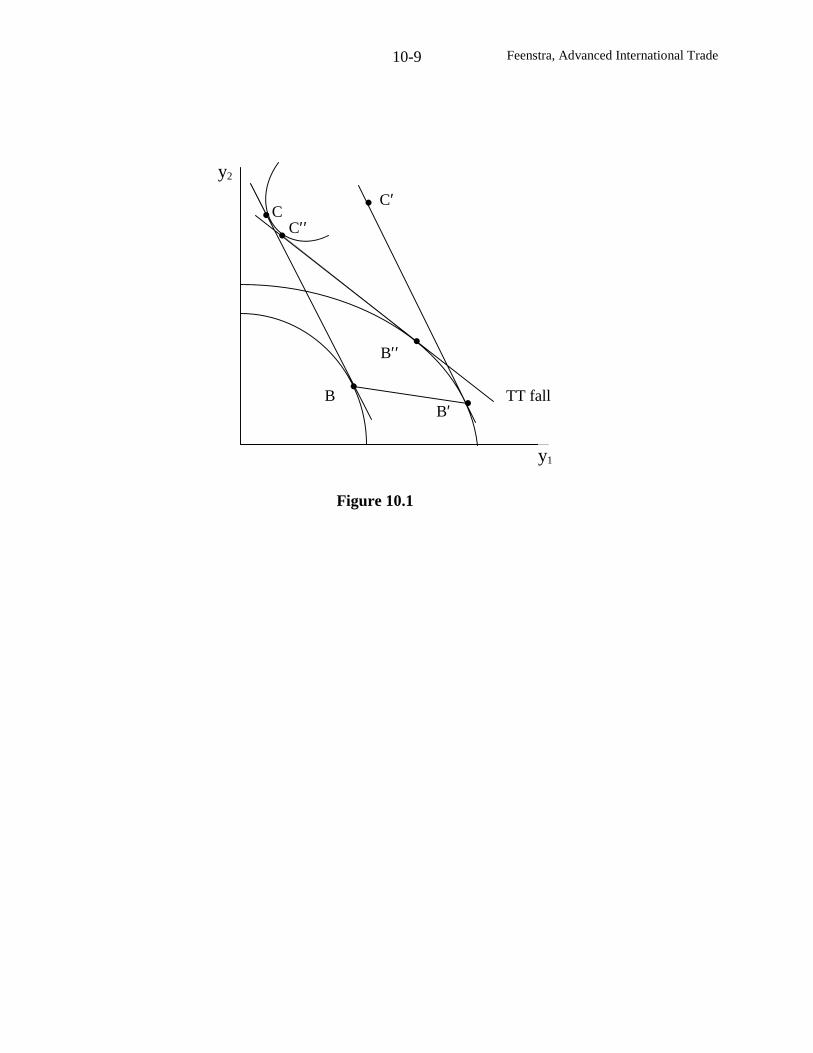
Feenstra, Advanced International Trade10-9
C′C
C′′
BB′
B′′
y2
TT fall
y1
Figure 10.1
Feenstra, Advanced International Trade10-10
example, α can represent a factor endowment or technological progress in some industry. The
total change in GDP is measured by:
αα∂
∂+∂∂= d
Gdp
p
GdG = y1dp + α
α+
αd
d
dy
d
dyp 21 . (10.7)
We presume that
α+
α=
α∂∂
d
dy
d
dyp
G 21 andαd
dy1 are both positive, meaning that growth at
constant prices increases both GDP and production of the exportable.
As in chapter 7, we will allow for different consumers but suppose that the numeraire
good is additively separable in consumption, so that consumer utilities can be summed. Total
social welfare is then )],p(G,p[W α , which serves as an indirect utility function for the
economy, where 1cp/W −=∂∂ is the (negative of) consumption of good 1 and 1G/W ≡∂∂ .
Then social welfare is constant due to growth if and only if,
0dG
dp)cy(dG
dpp
Gdp
p
WdW 11 =α
α∂∂+−=
α
α∂∂+
∂∂+
∂∂= . (10.8)
Thus, the drop in the export price that will just keep welfare constant is,
)yc(dG
dp 11 −αα∂
∂= . (10.9)
Next, we solve for the equilibrium change in the relative price of exports and compare
that to (10.9). Equilibrium in the export market means that *111 m)cy( =− , where *
1m is import
demand from the rest of the world. Totally differentiating this, we obtain,
Feenstra, Advanced International Trade10-11
dpdp
dmdp
p
c
p
yd
d
dy *1111 =
∂∂−
∂∂+α
α.
Thus, the equilibrium change in the price of exports is,
∂∂
−∂∂
−
αα=
p
c
p
y
dp
dm
dd
dy
dp11
*1
1
. (10.10)
The denominator of (10.10) is negative while the numerator is positive, so this expression
indicates the drop in the export price due to growth. Welfare is constant if (10.9)=(10.10), and
welfare falls if (10.10) < (10.9). This will occur if and only if,
−
∂∂
−∂∂
>α∂
∂−α dp
dm
p
c
p
yG)cy(
d
dy *111
111 .
Dividing this equation through by *111 m)cy( =− , and making use of
α+
α=
α∂∂
d
dy
d
dyp
G 21 , we
can express this necessary and sufficient condition for immiserizing growth as,
−
∂∂−
∂∂>
α+
αα *1
*1
*1
11211
m
p
dp
dm
m
p
p
c
p
y
d
dy
d
dyp
d
dyp . (10.11)
To interpret this expression, note that the first term on the right is the elasticity of export
supply and is positive. For immiserizing growth to occur, it is therefore necessary that the term
on the left exceed the amount
−
*1
*1
m
p
dp
dm, which is the elasticity of foreign demand for
Feenstra, Advanced International Trade10-12
imports. If this elasticity is less than unity, i.e. foreign demand is inelastic, then immiserizing
growth can occur even when the expression on the left of (10.11) is also less than unity.
However, if foreign demand for imports is elastic, then for (10.11) to be satisfied it must also be
the case that the expression on the left exceeds unity. By inspection, this occurs if and only if
dy2/dα < 0, that is, when growth reduces the output of good 2 (at constant prices). Summarizing
these results, we have:
Theorem (Bhagwati, 1958)
Immiserizing growth occurs if and only if (10.11) holds. Necessary conditions for this are that
either: (a) the foreign demand for imports is inelastic, or (b) growth reduces the output of the
importable good (at constant prices).
Condition (a) is not surprising, since having inelastic demand for a product is the same
condition that would permit farmers to be worse off after a bumper crop, as in the example given
in introductory economics textbooks. What is more surprising is that immiserizing growth can
occur even when foreign demand is not inelastic, but this requires that condition (b) hold, i.e. that
growth reduces the output of the importable good. We know from the Rybczynski Theorem that
this condition would hold in the two-by-two model if the factor used intensively in exports has
grown. So this is one scenario when immiserizing growth can occur. Are there others?
Findlay and Grubert (1959) answer this question in the affirmative. They considered
Hick’s neutral technological progress in good 1. To demonstrate the effects of this, we work
with the GDP function, defined as:
Feenstra, Advanced International Trade10-13
Vvvsubject to)v(f)v(pAf)V,Ap(G 21210iv
max =++≡≥
. (10.12)
That is, the parameter α that appeared in the earlier GDP function now equals A, which is the
Hick’s neutral productivity parameter on good 1. Notice that Ap enters in a multiplicative form
as an argument of the GDP function, since that is how it appears in the objective function.
We have demonstrated in chapter 1 that the derivative of the GDP function with respect
to price equals the output of that good, or 1yp/G =∂∂ . Letting G1(Ap,V) denote the partial
derivative of G with respect to its first argument, we therefore have:
A)V,Ap(Gdp
)Ap(d
)Ap(
G
p
Gy 11 =
∂∂=
∂∂= . (10.13)
Differentiating this expression again, it follows that:
,A)V,Ap(G]A)V,Ap(G[pp
y 2111
1 =∂∂=
∂∂
(10.14a)
and,
.Ap)V,Ap(G)V,Ap(G]A)V,Ap(G[AA
y1111
1 +=∂∂=
∂∂
(10.14b)
Converting these expressions into elasticity form, we readily obtain,
1
1
1
211
1
1
1
1
y
p
p
y1
y
pAG
y
A)V,Ap(G
y
A
A
y
∂∂+=+=
∂∂
, (10.15)
where the first equality is obtained from (10.14b), and the second from (10.13) and (10.14a).
Feenstra, Advanced International Trade10-14
We know that 0p/y1 ≥∂∂ , and will presume that 0p/y1 >∂∂ . It follows immediately
that 1)y/A)(A/y( 11 >∂∂ . That is, in a two-by-two economy, Hick’s neutral technological
progress in a good will raise its output by more than the increase in productivity. This result is
obtained because the rise in productivity will increase factor prices in an industry, thereby
attracting resources from the rest of the economy. This is illustrated in Figure 10.2, where with
unchanged inputs industry 1 would expand by A due to the technological progress, but after
attracting resources from the rest of the economy it expands by 1y > A . Moreover, as illustrated
in Figure 10.2, this will imply that output in industry 2 must contract, because it is losing factor
inputs. Thus, there is a “Rybczynski-like” effect at work even when the source of growth is
neutral technological progress in one industry, leading to a contraction of the other industry (at
constant prices). This type of growth therefore satisfies condition (b) of the above theorem,
making immiserizing growth possible.
The result in (10.12) that the GDP function should have price multiplied by the Hick’s
neutral productivity parameter in each industry was already used in chapter 3 (see equation 3.24),
where we reviewed the work of Harrigan (1997). He estimated a translog GDP function over the
OECD countries while allowing for technology to differ across countries. Industry prices were
treated as equal across countries (due to free trade), so it was only the technology parameters and
factor endowments that appeared in the GDP function. The result in (10.15) that the elasticity of
output with respect to each industry’s productivity exceeds unity then becomes a testable
hypothesis: it will hold empirically provided that certain parameters of the translog GDP
function satisfy appropriate conditions.8 Thus, by estimating the GDP function we are able to
test this result of Findlay and Grubert (1959).
8 See problem 10.2.
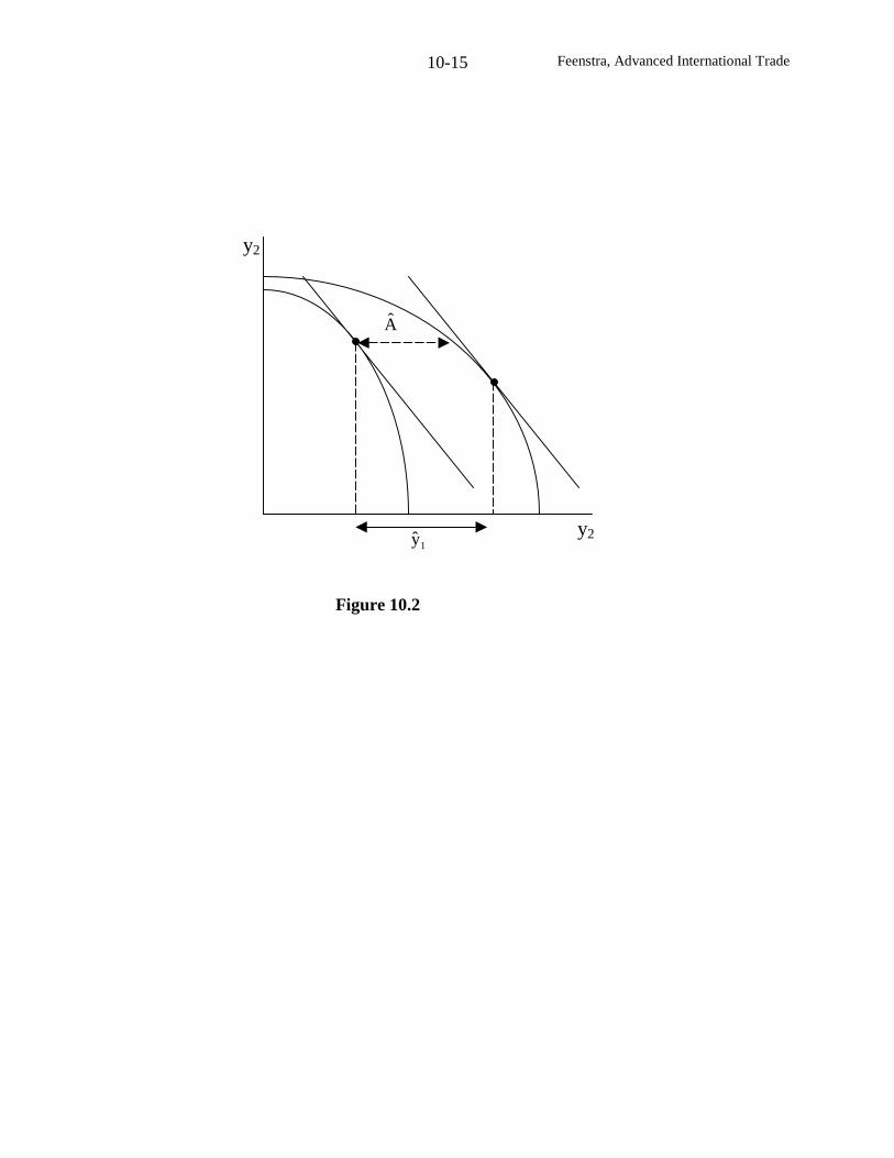
Feenstra, Advanced International Trade10-15
A
1y
Figure 10.2
y2
y2
Feenstra, Advanced International Trade10-16
Endogenous Growth
Our discussion in the previous section did not model growth in any meaningful way, but
simply treated it as a comparative statics increase in productivity or a factor endowment.
Obviously, this is unsatisfactory. The celebrated model of Solow (1956) specified that capital
accumulation should depend on investment, which equals to savings in the autarky one-sector
economy, so that capital would gradually rise to its steady-state level. But that model still
assumed that technological progress was exogenous, and a positive rate of technological progress
or growth in the labor force was needed to obtain steady-state growth. The same assumptions
were used in two-sector, open economy versions of this model, such as Smith (1977).
Ultimately, interest in the profession has turned to models that instead allow for an endogenous
rate of technological innovation, and we shall outline one of these models, taken from Grossman
and Helpman (1990; 1991, chapters 3, 8 and 9).
Many of the “endogenous growth” models build upon the monopolistic competition
framework we introduced in chapter 5, but rather than thinking of differentiated final products,
we instead consider differentiated intermediate inputs. The idea is that an increase in the variety
(N) of differentiated inputs will allow for an increase in output, much like an increase in variety
of final goods allowed for higher consumer utility in chapter 5.9 To make this precise, suppose
that there is a single final good, with output y, produced with the CES production function:
)1/(N
1i
/)1(ixy
−σσ
=
σ−σ
= ∑ (10.16)
where xi is the quantity of input variety i = 1,…,N. As usual, we assume σ > 1, so that it is
9 See problem 5.1. The use of differentiated inputs to generate economy-wide returns to scale is often attributed toEthier (1979).
Feenstra, Advanced International Trade10-17
meaningful to think of changes in the number of inputs.10
If inputs are all priced equally in equilibrium, then their quantities are also equal, xi = x,
and so (10.16) can be rewritten as,
XNxNy )1/(1)1/( −σ−σσ == , (10.17)
with NxX ≡ . We can think of X as the “aggregate” amount of the intermediate input, and
holding this magnitude fixed, (10.17) shows that increases in N raise output y (since σ > 1).
This amounts to a productivity gain in the final good industry, due to the proliferation of
differentiated intermediate inputs. Indeed, we could re-label )1/(1N −σ on the right of (10.17) as
“A” to obtain the simple production function y = AX, where technological progress A will
depend on the number of new inputs.11 By carefully modeling the dynamics of how N evolves
due to the entry of new firms, we therefore have a story of endogenous technological progress, or
endogenous growth.
Autarky Equilibrium
We begin by describing the autarky equilibrium. The price of the final good at each point
in time is P(t). If the consumer spends E(t) on this good, then the quantity Y(t) = E(t)/P(t) will
be purchased, and we assume that this provides instantaneous utility of lnY(t) = lnE(t) – lnP(t).
The consumer’s problem is then:
∫∞ −τρ−
τττ−τ
t)t(
)(Ed)](Pln)(E[lnemax , (10.18)
10 If σ < 1, then output is zero whenever any input is zero. Thus, all inputs are essential to production, and wecannot think of introducing new inputs. In contrast, when σ > 1, then output will increase by a finite amount whennew inputs are introduced, as shown in (10.17).11 This is like the so-called “y = AK” production function used in some macroeconomic models.
Feenstra, Advanced International Trade10-18
subject to the budget constraint:
∫∞ −τ− ττ
t)]t(R)(R[ d)(Ee ∫
∞ −τ− +ττ≤t
)]t(R)(R[ )t(BLd)(we , (10.19)
where R(t) is the cumulative interest rate from time 0 to time t, so that dt/dR)t(R ≡& is the
instantaneous interest rate. This budget constraint states that the discounted value of labor
income w(t)L, plus initial assets B(t), cannot exceed the discounted value of expenditure. The
solution to this optimization problem is,12
ρ−= RE
E &&
, (10.20)
where we omit the time index on variables when this will not cause confusion.
Condition (10.20) states that when the nominal interest rate R& exceeds the consumer’s
discount rate then expenditure is rising. This is because with a high interest rate it is optimal to
put a large amount of assets into savings initially, and gradually increase consumption thereafter.
Generally, the nominal interest )t(R& will depend on the normalization made on prices.
Grossman and Helpman (1990, 1991) choose the normalization E(t) ≡1, which implies from (20)
that )t(R& ≡ ρ, as we shall also use.
On the production side, the final good y is manufactured under perfect competition with
the production function (10.17), where xi is the quantity of each of N intermediate inputs (all
these variables depend on t). These inputs are produced under monopolistic competition, and
each unit of xi requires one unit of labor, which is the only input. It follows that the price of each
11 As solved for in problem 10.3.
Feenstra, Advanced International Trade10-19
input is,
−σσ==
σ−
1wpor,w
11p ii , (10.21)
where w is the wage (which depends on t).
Input-producing firms have a fixed cost only when they begin production. The key
question is: how should this fixed cost be modeled? If we presume that the fixed cost is a
fixed amount of labor α, as in the static monopolistic competition model, then there will be a
limit to the number of products that could be profitably developed. In other words, growth of
inputs N(t) will cease at some point in time. The first dynamic monopolistic competition models
had this feature (Judd, 1985, Grossman and Helpman, 1989), while the work of Romer (1990)
and Grossman and Helpman (1990, 1991) avoided this outcome by presuming that fixed costs
are inversely proportional to the number of products already developed, so that fixed labor costs
are α/N(t). The idea is that the creation of products contributes to a “public stock of
knowledge,” which makes the invention of new products even easier. Notice that in a two-
country model, this will allow for the potential spillover of public knowledge across borders,
which will turn out to be very important.
With fixed labor costs of α/N(t), the nominal fixed costs are αw(t)/N(t). These are
financed by consumers purchasing equity in the firms, which provides both dividends and capital
gains. The instantaneous profits of the firms are:
wx1
1x)wp( iii
−σ=−=π , (10.22)
using (10.21) and symmetry of the equilibrium, so that xi = x. The zero profit conditions for the
Feenstra, Advanced International Trade10-20
firms are that the present discounted value of instantaneous profits in (10.22) must equal the
fixed costs αw(t)/N(t),
)t(N
)t(wd)(x)(w
1
1e)t(V
t)t( α=τττ
−σ≡ ∫
∞ −τρ− , for all t. (10.23)
Since (10.23) holds for all t, we can differentiate it with respect to t, obtaining,
2t)t(
N
Nw
N
wd)(x)(w
1
1e)t(x)t(w
1
1V
&&& α−α=τττ
−σρ+
−σ−= ∫
∞ −τρ− . (10.24)
To simplify (10.24), we can divide by the fixed costs αw/N, obtaining,
{rateinterest
gainsCapital
V/VDividends
costFixed/
N
N
w
wNx
1
1 ρ=
−+
α
−σπ
43421
43421
&&
4342143421
&
. (10.25)
This is the key arbitrage condition of the endogenous growth model with expanding input
variety, as derived by Grossman and Helpman (1990, 1991). The left-hand side of (10.25) is the
sum of dividends plus capital gains, which should equal the discount rate on the right, that we
interpret as the real interest rate.
With (10.25) in hand we can complete the model quite easily by using the full-
employment condition for the economy. This can be written as,
NN
NxL &
α+= . (10.26)
The left-hand side of (10.26) is the fixed endowment of labor, and the right-hand side equals the
sum of labor used in production, Nx = X, and labor used in R&D, which is the fixed cost (α/N)
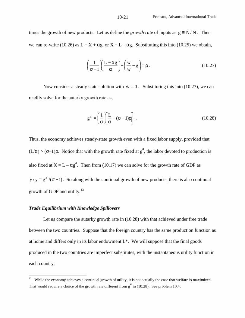
Feenstra, Advanced International Trade10-21
times the growth of new products. Let us define the growth rate of inputs as N/Ng &≡ . Then
we can re-write (10.26) as L = X + αg, or X = L – αg. Substituting this into (10.25) we obtain,
ρ=
−+
αα−
−σg
w
wgL
1
1 &. (10.27)
Now consider a steady-state solution with 0w =& . Substituting this into (10.27), we can
readily solve for the autarky growth rate as,
ρ−σ−α
σ= )1(
L1ga . (10.28)
Thus, the economy achieves steady-state growth even with a fixed labor supply, provided that
(L/α) > (σ–1)ρ. Notice that with the growth rate fixed at ga, the labor devoted to production is
also fixed at X = L – αga. Then from (10.17) we can solve for the growth rate of GDP as
)1/(gy/y a −σ=& . So along with the continual growth of new products, there is also continual
growth of GDP and utility.13
Trade Equilibrium with Knowledge Spillovers
Let us compare the autarky growth rate in (10.28) with that achieved under free trade
between the two countries. Suppose that the foreign country has the same production function as
at home and differs only in its labor endowment L*. We will suppose that the final goods
produced in the two countries are imperfect substitutes, with the instantaneous utility function in
each country,
13 While the economy achieves a continual growth of utility, it is not actually the case that welfare is maximized.
That would require a choice of the growth rate different from ga
in (10.28). See problem 10.4.
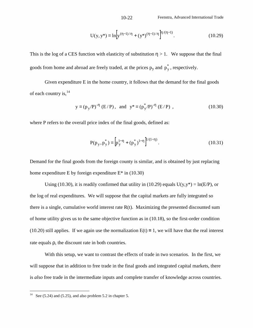
Feenstra, Advanced International Trade10-22
[ ] )1/(/)1(/)1( *)y(yln*)y,y(U−ηηη−ηη−η += . (10.29)
This is the log of a CES function with elasticity of substitution η > 1. We suppose that the final
goods from home and abroad are freely traded, at the prices py and *yp , respectively.
Given expenditure E in the home country, it follows that the demand for the final goods
of each country is,14
)P/(E/P)p(y -y
η= , and )P/(E/P)p(y* -*y
η= , (10.30)
where P refers to the overall price index of the final goods, defined as:
[ ] )1/(11*y
1y
*yy )p(p)p,p(P
η−η−η− += . (10.31)
Demand for the final goods from the foreign county is similar, and is obtained by just replacing
home expenditure E by foreign expenditure E* in (10.30)
Using (10.30), it is readily confirmed that utility in (10.29) equals U(y,y*) = ln(E/P), or
the log of real expenditures. We will suppose that the capital markets are fully integrated so
there is a single, cumulative world interest rate R(t). Maximizing the presented discounted sum
of home utility gives us to the same objective function as in (10.18), so the first-order condition
(10.20) still applies. If we again use the normalization E(t) ≡ 1, we will have that the real interest
rate equals ρ, the discount rate in both countries.
With this setup, we want to contrast the effects of trade in two scenarios. In the first, we
will suppose that in addition to free trade in the final goods and integrated capital markets, there
is also free trade in the intermediate inputs and complete transfer of knowledge across countries.
14 See (5.24) and (5.25), and also problem 5.2 in chapter 5.
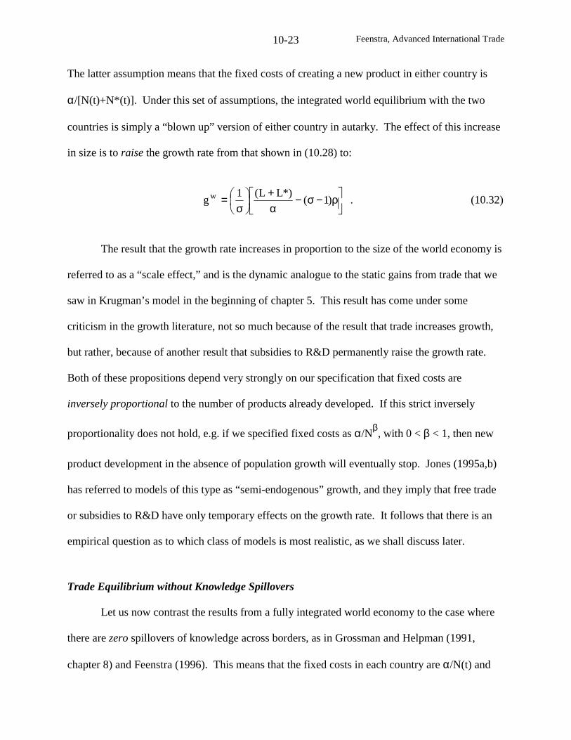
Feenstra, Advanced International Trade10-23
The latter assumption means that the fixed costs of creating a new product in either country is
α/[N(t)+N*(t)]. Under this set of assumptions, the integrated world equilibrium with the two
countries is simply a “blown up” version of either country in autarky. The effect of this increase
in size is to raise the growth rate from that shown in (10.28) to:
ρ−σ−
α+
σ= )1(
*)LL(1g w . (10.32)
The result that the growth rate increases in proportion to the size of the world economy is
referred to as a “scale effect,” and is the dynamic analogue to the static gains from trade that we
saw in Krugman’s model in the beginning of chapter 5. This result has come under some
criticism in the growth literature, not so much because of the result that trade increases growth,
but rather, because of another result that subsidies to R&D permanently raise the growth rate.
Both of these propositions depend very strongly on our specification that fixed costs are
inversely proportional to the number of products already developed. If this strict inversely
proportionality does not hold, e.g. if we specified fixed costs as α/Nβ, with 0 < β < 1, then new
product development in the absence of population growth will eventually stop. Jones (1995a,b)
has referred to models of this type as “semi-endogenous” growth, and they imply that free trade
or subsidies to R&D have only temporary effects on the growth rate. It follows that there is an
empirical question as to which class of models is most realistic, as we shall discuss later.
Trade Equilibrium without Knowledge Spillovers
Let us now contrast the results from a fully integrated world economy to the case where
there are zero spillovers of knowledge across borders, as in Grossman and Helpman (1991,
chapter 8) and Feenstra (1996). This means that the fixed costs in each country are α/N(t) and
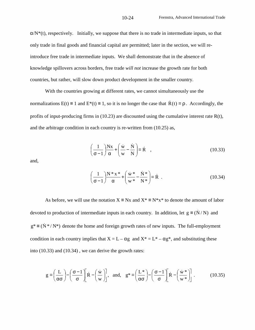
Feenstra, Advanced International Trade10-24
α/N*(t), respectively. Initially, we suppose that there is no trade in intermediate inputs, so that
only trade in final goods and financial capital are permitted; later in the section, we will re-
introduce free trade in intermediate inputs. We shall demonstrate that in the absence of
knowledge spillovers across borders, free trade will not increase the growth rate for both
countries, but rather, will slow down product development in the smaller country.
With the countries growing at different rates, we cannot simultaneously use the
normalizations E(t) ≡ 1 and E*(t) ≡ 1, so it is no longer the case that ρ=)t(R& . Accordingly, the
profits of input-producing firms in (10.23) are discounted using the cumulative interest rate R(t),
and the arbitrage condition in each country is re-written from (10.25) as,
RN
N
w
wNx
1
1 &&&
=
−+
α
−σ, (10.33)
and,
R*N
*N
*w
*w*x*N
1
1 &&&
=
−+
α
−σ. (10.34)
As before, we will use the notation X ≡ Nx and X* ≡ N*x* to denote the amount of labor
devoted to production of intermediate inputs in each country. In addition, let )N/N(g &≡ and
*)N/*N(*g &≡ denote the home and foreign growth rates of new inputs. The full-employment
condition in each country implies that X = L – αg and X* = L* – αg*, and substituting these
into (10.33) and (10.34) , we can derive the growth rates:
−
σ−σ−
ασ=
w
wR
1Lg
&& , and,
−
σ−σ−
ασ=
*w
*wR
1*L*g
&& . (10.35)
Feenstra, Advanced International Trade10-25
These equations show that the growth rates are inversely related to the real interest rates
)]w/w(R[ && − and *)]w/*w(R[ && − : having a higher nominal interest rate R& lowers the
discounted value of profits and therefore expenditure on R&D; conversely, having a rising path
of wages and prices leads to rising profits and a lower real interest rate, with higher R&D.
Taking the difference between the two growth rates in (10.35), we obtain,
−
σ−σ+
ασ−=−
*w
*w
w
w1*LL*gg
&&. (10.36)
Let us assume henceforth that the home country is larger, L > L*. From (10.36) we see
that this difference in size will tend to be associated with a faster growth rate at home, g > g*.
The growth rates are also affected, however, by the change in wages on the right. In the autarky
equilibrium discussed above, we had focused on the steady-state solution with 0w =& . But now
it is impossible to assume this for both countries: assuming 0*ww == && implies that *gg >
from (10.36), and we will argue below that this implies rising relative wages for the home
country, *w/*ww/w && > , which is a contradiction. Thus, the assumption of a steady-state
equilibrium is inconsistent with the dynamic equations for the two countries. Accordingly, we
need to solve for the growth rates outside of the steady state.
We begin by solving for the change in wages, from the production function
XNy )1/(1 −σ= in (10.17), where X is the amount of intermediate inputs purchased at the price of
pi = wσ/(σ – 1). It follows that the marginal cost of producing the final good is
]N)1/[(wN/pp )1/(1)1/(1iy
−σ−σ −σσ== at home, and ]*)N)(1/[(*wp )1/(1*y
−σ−σσ= abroad.
Differentiating these and taking the difference, we obtain,
Feenstra, Advanced International Trade10-26
−σ−−
−=
−
1
*gg
*w
*w
w
w
p
p
p
p*y
*y
y
y &&&
&
&. (10.37)
This equation states that a higher growth rate at home will tend to be associated with rising
relative wages, but this also depends on the changes in the prices of the final goods in each
country.
To determine these prices, we make use of the CES demands in (10.30), which imply
that η= -1/*yy (y/y*))/pp( . Differentiating this using the production functions XNy )1/(1 −σ= and
*X*)N(*y )1/(1 −σ= , we obtain,
−+
−σ−
η−=
−
*X
*X
X
X
1
*gg1
p
p
p
p*y
*y
y
y &&&
&
&. (10.38)
Then combining (10.36) – (10.38), we can derive the fundamental relation,
−
ησ−σ∆−
ασ−∆=−
*X
*X
X
X1*LL*gg
&&, (10.39)
where,
1)1(
11
>
ησ−η−≡∆
−
. (10.40)
Equation (10.39) shows that the difference in the growth of new inputs across the
countries depends on the difference in their size. There is also another term on the right of
(10.39), depending on X& and *X& , but we can safely presume that this term approaches zero as
∞→t . Notice that the difference in the autarky growth rates of the two countries is exactly
Feenstra, Advanced International Trade10-27
(L – L*)/ασ, but in (10.39), the limiting growth rates of the countries will differ by this times the
amount ∆>1. Therefore, in the absence of knowledge spillovers the effect of trade is to magnify
the initial difference in the growth rates of the two countries.
We have not yet determined whether trade will increase the growth rate of the large
country, or slow down the growth rate of the small country. Some additional calculations show
that the first case is not possible: the growth rate of the large country must approach its autarky
rate of ga
as ∞→t .15 Our results are then summarized by:
Theorem (Feenstra, 1996)
(a) at
lim gg =∞→
, which equals the autarky growth rate ga
of the large country;
(b) =∞→
*gt
lim ∗ag
ασ−−∆− *LL
)1( , which is less than the autarky growth rate ∗ag of the small
country, ∗ag σρ−σ−α= /])1()/*L[( ;
(c) 0*w
*w
w
wt
lim >
−
∞→
&&, and 0
p
p
p
p*y
*y
y
y
t
lim <
−
∞→
&&.
Parts (a) and (b) of this theorem have already been discussed above. The results in (c)
follow from substituting the limiting growth rates into (10.37) and (10.38). Relative wages move
in favor of the larger country, which reflects the rising productivity of that country due to the
faster-growing number of intermediate inputs. But this same efficiency gain leads to a fall in the
relative price of final goods. These different wage and price movements emphasize how difficult
15 See problem 10.5.
Feenstra, Advanced International Trade10-28
it is to make a general prediction of the terms of trade movement in this model: it depends on
which goods/factors are used to measure the terms of trade.
The finding that the small country has its rate of product development slowed down does
not necessarily translate into a welfare loss, though it might. That will depend on whether
intermediate inputs are traded or not. Initially continue with our assumption that inputs are not
traded. The welfare obtained by consumers in the small country will depend, of course, on the
price index )p,p(P *yy for purchases of the final goods. Let us choose the foreign wage as the
numeraire, w* ≡ 1. Then since the number of intermediate inputs produced abroad is slowed
down by trade, the price of its final good *yp is higher than in autarky. This will create a
potential welfare loss. But the foreign consumers also have the final good from the home
country available, which creates a potential welfare gain. Which of these effects dominate will
depend on a comparison of elasticities: if η > (σ+1), then there is an overall welfare gain; but if
η < (σ+1), then there is a potential welfare loss.16
What about when the intermediate inputs are traded? Then the argument is quite
different. Despite the fact that product development has been slowed in the small country, it can
still purchase intermediate inputs from abroad. For t sufficiently large, it will definitely be the
case that the efficiency gain from the additional imported inputs more than offsets the loss from
the reduced number of local inputs, so that the price of the final good *yp is lower than in
autarky. Thus, consumers in the small country benefit from a reduction in the price of their own
16 Specifically, Feenstra (1996, Proposition 2) finds that the price index under free trade exceeds that under autarkyfor t sufficiently high when η < (σ+1), and a weak additional condition is satisfied. The finding that welfare in thesmaller country can potentially fall is related to the fact that R&D is being undertaken at less than the sociallyoptimal rate in autarky, as demonstrated in problem 10.4. Then trade in final goods but not in intermediate inputsworsens that distortion in that country. Markusen (1989) also discusses how trade in final goods, but not inintermediate inputs, can lead to a welfare loss even in a static model.
Feenstra, Advanced International Trade10-29
final good as well as the imported final good, so there are welfare gains for both reasons.
It is worth emphasizing that our finding that trade can slow down the rate of product
development occurs only when there are zero spillovers of knowledge. Provided that there are
some positive spillovers, then Grossman and Helpman (1991, chapter 9) and Rivera-Batiz and
Romer (1991a,b) argue that product innovation in both countries will increase. Indeed, this
occurs even if knowledge spillovers are the only international flows, without any trade in final
goods or inputs. So the assumption of zero international spillovers we have used above is an
extreme case, but it serves to highlight how important these spillovers are to growth.
Empirical Evidence
Importance of Size
The first implication of the endogenous growth models is that “size matters” for growth.
This follows directly from the equation for autarky growth rates in (10.28), where a higher labor
stock (measured in units of effective R&D workers, or L/α) leads to a higher growth rate. This
implication is analogous to what we found in Krugman’s static model reviewed at the beginning
of chapter 5: doubling a country’s size would lead to efficiency gains through economies of
scale, and additional consumer gains through increased variety. In the dynamic model outlined
above, increasing a country’s size leads to increased variety of intermediate inputs, which results
in efficiency gains in producing the final good and also reduces the fixed costs α/N(t) of
inventing new inputs. The latter reduction in fixed costs is what leads to a permanently higher
growth rate due to larger country size.
How realistic is this result? Over very long time periods, it is perhaps reasonable to think
that economies will growth in proportion to their size. Kremer (1993) considers the period from
Feenstra, Advanced International Trade10-30
one million B.C. to the present, and finds that the growth rate of population is proportional to its
level. On the other hand, over shorter time spans, the implications of the “scale effect” in the
endogenous growth model do not find support. Jones (1995a,b) proposes a direct test of
endogenous growth, whereby changes in policy should have permanent effects on the growth
rate, and this hypothesis is decisively rejected on data for the U.S. and other advanced countries.
As we discussed earlier, these negative results led Jones to propose the “semi-endogenous”
growth model, and there is now a class of growth models that operate without the scale effect.17
International Trade and Convergence
The second implication of the endogenous growth model was that, with international
spillovers of knowledge, trade should increase growth rates. There is an active debate over
whether this hypothesis holds empirically. Advocates of this view includes Dollar (1992), Sachs
and Warner (1995), Edwards (1998), Ben-David (1993, 1996, 2001), and Frankel and Romer
(1999). But these empirical results are all dismissed by Rodriguez and Rodrik (2000), and more
specific criticisms on individual papers are made by Harrison (1996) and Slaughter (2001). In
order to evaluate these papers, it is useful to first relate them to another line of empirical
research dealing with the convergence of countries to their steady-state growth rates.
The convergence literature is not motivated by the endogenous growth models at all, but
rather, by the exogenous growth model such as Solow (1956) and extensions thereof. In those
models, all countries converge to the same steady-state growth rate, but this still allows for
different levels of GDP per-capita (depending on characteristics of the countries). So countries
that are below their steady-state level of GDP per-capita should grow faster, and conversely,
countries that are above their steady-state GDP per-capita should grow slower, so as to approach
17 See Dinopoulos and Segerstrom (1999a) and Dinopoulos and Syropoulos (2001) for applications to trade.
Feenstra, Advanced International Trade10-31
the steady state. This property follows directly from the diminishing marginal product of capital.
There is both convergence in growth rates, and some degree of convergence in GDP per-capita
(though not necessarily to the same level across countries), and these two criterion tend to be
used interchangably. The same is true for the papers dealing with trade, which examine either
the impact on growth rates or on GDP per-capita across countries.
From the initial work of Barro (1991) and Barro and Salai-i-Martin (1991, 1992) the
convergence hypothesis found strong empirical support. This was also demonstrated by
Mankiw, Romer and Weil (1992), and led them to conclude that the original Solow model,
suitably extended to allow for human capital, is “good enough” at explaining cross-country
differences in growth rates: the endogenous growth models are apparently not needed! These
findings have been questioned in subsequent work, however, that consider a broader range of
countries. For example, Easterly and Levine (2000) emphasize that there has been divergence in
the absolute levels of income per-capita across countries: the rich have grown richer and some
of the poorest countries have become even poorer.18
A similar approach to assessing the effects of trade is taken by the authors cited above.
Sachs and Warner (1995) group their countries into two groups, one of which has an “open”
trade regime and the other of which is judged to be “closed.” Within the open group, they find
evidence of convergence, with the poorer countries growing faster, but this is not true for those
countries with closed trade regimes. By this argument, openness leads to convergence of
incomes across countries. Ben-David (1993, 1996, 1998) does a grouping of countries based on
their membership in regional trade agreements, or by the strength of their bilateral trade ties. He
also finds significant evidence of income convergence within these groups, but not necessarily
18 Bernanke and Gürkaynak (2001) also question the conclusions of Mankiw, Romer and Weil.
Feenstra, Advanced International Trade10-32
across the groups. Dollar and Kraay (2001a,b) contrast the experience of a group of developing
countries that have become more open (including China and India) with other developing
countries. They argue that growth in the former group is explained by openness and has
particularly benefited the poor. As noted above, all these papers are subject to some empirical
criticisms: among other difficulties, openness itself is fundamentally endogenous. Frankel and
Romer (1999) deal with this endogeneity by first estimating a gravity equation, and then
demonstrating that the predicted trade shares from this equation are indeed significant in
explaining income per-capita.
The finding that convergence occurs within groups, but not across groups, presents a
challenge to the exogenous growth models. But this finding is in the spirit of the endogenous
growth model without knowledge spillovers, discussed above, where the two countries
converged to different growth rates. In a more general multi-country growth model that
incorporates trade, Ventura (1997) also finds this result. In his model, capital does not have a
diminishing marginal product due to Rybczynski effects: increases in capital raises the output of
the capital-intensive good, and at fixed product prices, does not result in a reduced rental.
Nevertheless, Ventura shows that in the global equilibrium, there is convergence to steady-state
growth rates that differ across countries. The reason for convergence is that countries with
expanding capital will have falling equilibrium prices for their capital-intensive goods, and
therefore, a falling rental due to the Stolper-Samuelson theorem. So there is a general-
equilibrium linkage between capital accumulation and the rental, even though there are no
diminishing returns with fixed prices.
We might think of the model in Ventura (1997) as offering a third type of growth model,
in which there is neither dimishing returns to capital as in the Solow model; nor endogenous
Feenstra, Advanced International Trade10-33
growth due to increased input variety; but growth without dimishing returns due to Rybczynski
effects. Findlay (1996) argues that this framework may well be the most relevant one to analyze
the growth experience of developing countries, and these articles are recommended for further
reading.
Spillovers of Knowledge
A third area of empirical investigation is international spillovers of knowledge. It is clear
from our discussion above that these are crucial: gains from trade are much more likely when
knowledge flows across borders. Coe and Helpman (1995) test for the presence of such
spillovers using data for the OECD countries.19 Their hypothesis is that if international
spillovers occur, then the growth rates of countries should be correlated with both their own
R&D expenditures and also the R&D expenditures of their trading partners. Thus, they construct
measures of each country’s R&D expenditures, and weight these using bilateral import shares to
obtain an estimate of partner countries’ R&D expenditures. They find that TFP growth rates at
the country level are indeed correlated with own and partner-country R&D expenditures, lending
support to the idea that research and development carried out in one country “spills over” to its
trading partners.
An econometric difficulty with the Coe and Helpman estimates is that the TFP growth
rates and R&D expenditures are very likely to exhibit unit-roots in their time series behavior. In
that case, regressions of TFP on R&D could lead to estimates that are significantly different from
zero using conventional t-tests, even though the relationship might be spurious. To investigate
this, Keller (1998) re-constructs the weighted R&D expenditures of the trading partners used by
19 Coe, Helpman and Hoffmaister (1997) expand the sample to include developing countries.
Feenstra, Advanced International Trade10-34
Coe and Helpman, but using random rather than actual import weights. He shows that this
measure still has a positive correlation with TFP, suggesting that the relationship has little to do
with trade, and may be spurious. The unit-roots problem can be corrected using recent panel co-
integration techniques, as done by Funk (2001). He finds that there is no significant relationship
between TFP growth and import-weighted R&D expenditures of partner countries. However, he
does find a significant relationship between TFP and export-weighted R&D expenditures of
partner countries, supporting the idea that exporters learn from their customers.
Keller (2002) has extended the results of Coe and Helpman using sectoral rather than
aggregate country data. He again constructs a weighted average of R&D expenditures in other
countries, but now uses the distance to each partner as the weight. Denoting the distance from
country i to j by dij, Keller weights the other countries’ R&D expenditures by
ijde δ− . The
parameter δ measures how quickly the impact of other countries’ R&D expenditures on TFP
diminishes with distance. In fact, this parameter turns out to be positive and highly significant,
implying that spillovers are quite highly localized. For the two closest countries in his sample,
Germany and the Netherlands, one dollar of R&D expenditure in Germany has 31% of the
impact on Dutch productivity as does one dollar R&D expenditure in the Netherlands. The
effects of foreign R&D are lower for all other countries; for example, the relative effect of
American R&D on Canada is only 4% of the value of Canadian R&D on its own productivity.
So Keller’s results provide evidence of R&D spillovers across borders that are precisely
estimated, but small.
Another way that spillovers of knowledge have been assessed is through the use of patent
data. There is a large literature that applies this technique to firms within a country, and
Branstetter (2001) has extended it to consider firms in both the U.S. and Japan. When firms
Feenstra, Advanced International Trade10-35
apply for a patent in the U.S., they must classify it in one or more product areas. Treat each
product area as a component of the vector Bi = (bi1,…,biK), where bik is the number of patents
taken out by firm i in product area k. For two firms i and j, we can use the correlation between
Bi and Bj as a measure of their proximity in technology space. Then we can construct a weighted
average of the R&D expenditures of other firms, using the proximity with firm i as the weights.
This gives us a measure of the potential spillovers from other firms. Branstetter constructs these
measures separately for spillovers from U.S. firms, and spillovers from Japanese firms.20
Together with each firm’s own R&D expenditures, these are regressed on a measure of each
firm’s performance (either number of patents taken out annually, or TFP growth), to determine
the importance of the various spillovers.
In his results, Branstetter (2001, p. 75) finds that spillovers are primarily intra-national in
scope. There are some regressions where Japanese firms benefit from the weighted R&D
activity of American companies, but this effect does not remain significant when the domestic
spillovers are included in the regression. Conversely, there is no evidence that American firms
benefit from the R&D activities of the Japanese. This raises the idea that knowledge spillovers
may be asymmetric, and presumably flow from the most technologically advanced country
outwards. In other work, Branstetter (2000) has explored whether Japanese firms that have
foreign affiliates in the U.S. act as a “conduit” for knowledge flows, i.e. whether there is a
greater spillover between these foreign affiliates and other American firms. It appears that this is
indeed the case, so that foreign investment increases the flow of knowledge spillovers both to
and from the investing Japanese firms.
20 Both measures are constructed using the patents that Japanese and American firms take out in the U.S.
Feenstra, Advanced International Trade10-36
Measuring Product Variety
All of the empirical applications we have discussed so far have been indirect tests of the
endogenous growth model, relying on hypotheses arising from it but not actually measuring the
variety of inputs. Our fourth and final empirical method will be to develop a direct test of
endogenous growth, by constructing a measure of input variety that is “exact” for the CES
production function, as in Feenstra (1994) and Feenstra and Markusen (1994). We show that this
measure of product variety is correlated with productivity growth.
Let us begin with the CES production function in (10.16). The problem with using this
function is that it is symmetric: at equal prices, every input would have the same demand. That
assumption is made for convenience in our theoretical models, but is unacceptable empirically:
we need to let demand be whatever the data indicates. So instead we will work with the non-
symmetric CES function,
1,xa)I,x(fy
)1/(
Ii
/)1(itittt
t
>σ
==
−σσ
∈
σ−σ∑ , (10.41)
where ai > 0 are parameters and It denotes the set of inputs available in period t, at the prices pit.
The CES unit-cost function dual to (10.41) is,21
σσ−
∈
σ− ≡>σ
= ∑ ii
)1/(1
Ii
1ititt ab1,,pb)I,p(c
t
. (10.42)
We are interested in determining how much unit-costs are reduced when the set of
product varieties expands. To this end, let us first consider the case where It-1 = It = I, so there is
21 This is analogous to the CES price index in (5.25), and see also problem 8.3 of chapter 8 to derive the CESdemand system in the non-symmetric case.
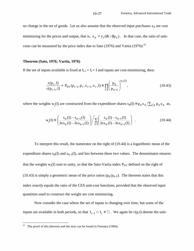
Feenstra, Advanced International Trade10-37
no change in the set of goods. Let us also assume that the observed input purchases xit are cost
minimizing for the prices and output, that is, )p/c(yx ittit ∂∂= . In that case, the ratio of unit-
costs can be measured by the price index due to Sato (1976) and Vartia (1976):22
Theorem (Sato, 1976; Vartia, 1976)
If the set of inputs available is fixed at It-1 = It = I and inputs are cost-minimizing, then:
=− )I,p(c
)I,p(c
1t
t ,p
p)I,x,x,p,p(P
)I(w
Ii 1it
itt1tt1tSV
i
∏∈ −
−−
≡ (10.43)
where the weights wi(I) are constructed from the expenditure shares sit(I) ≡ ∑ ∈ Ii itititit xpxp as,
wi(I) ≡
)I(sln–)I(sln
)I(s–)I(s
)I(sln–)I(sln
)I(s–)I(s
Ii 1itit
1itit
1itit
1itit ∑∈ −
−
−
−
. (10.44)
To interpret this result, the numerator on the right of (10.44) is a logarithmic mean of the
expenditure shares sit(I) and sit-1(I), and lies between these two values. The denominator ensures
that the weights wi(I) sum to unity, so that the Sato-Vartia index PSV defined on the right of
(10.43) is simply a geometric mean of the price ratios (pit/pit-1). The theorem states that this
index exactly equals the ratio of the CES unit-cost functions, provided that the observed input
quantities used to construct the weight are cost minimizing.
Now consider the case where the set of inputs is changing over time, but some of the
inputs are available in both periods, so that ∅≠∩− t1t II . We again let c(p,I) denote the unit-
22 The proof of this theorem and the next can be found in Feenstra (1994).
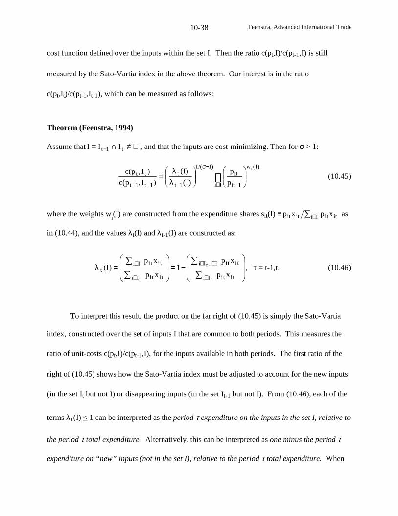
Feenstra, Advanced International Trade10-38
cost function defined over the inputs within the set I. Then the ratio c(pt,I)/c(pt-1,I) is still
measured by the Sato-Vartia index in the above theorem. Our interest is in the ratio
c(pt,It)/c(pt-1,It-1), which can be measured as follows:
Theorem (Feenstra, 1994)
Assume that ∅≠∩= − t1t III , and that the inputs are cost-minimizing. Then for σ > 1:
=−− )I,p(c
)I,p(c
1t1t
tt)I(w
Ii 1it
it)1/(1
1t
ti
p
p
)I(
)I(∏∈ −
−σ
−
λλ
(10.45)
where the weights wi(I) are constructed from the expenditure shares sit(I) ≡ ∑ ∈ Ii itititit xpxp as
in (10.44), and the values λt(I) and λt-1(I) are constructed as:
−=
=λ
∑
∑
∑
∑
τ
τ
τ ∈ ττ
∉∈ ττ
∈ ττ
∈ τττ
Ii ii
Ii,Ii ii
Ii ii
Ii ii
xp
xp1
xp
xp)I( , τ = t-1,t. (10.46)
To interpret this result, the product on the far right of (10.45) is simply the Sato-Vartia
index, constructed over the set of inputs I that are common to both periods. This measures the
ratio of unit-costs c(pt,I)/c(pt-1,I), for the inputs available in both periods. The first ratio of the
right of (10.45) shows how the Sato-Vartia index must be adjusted to account for the new inputs
(in the set It but not I) or disappearing inputs (in the set It-1 but not I). From (10.46), each of the
terms λτ(I) < 1 can be interpreted as the period τ expenditure on the inputs in the set I, relative to
the period τ total expenditure. Alternatively, this can be interpreted as one minus the period τ
expenditure on “new” inputs (not in the set I), relative to the period τ total expenditure. When
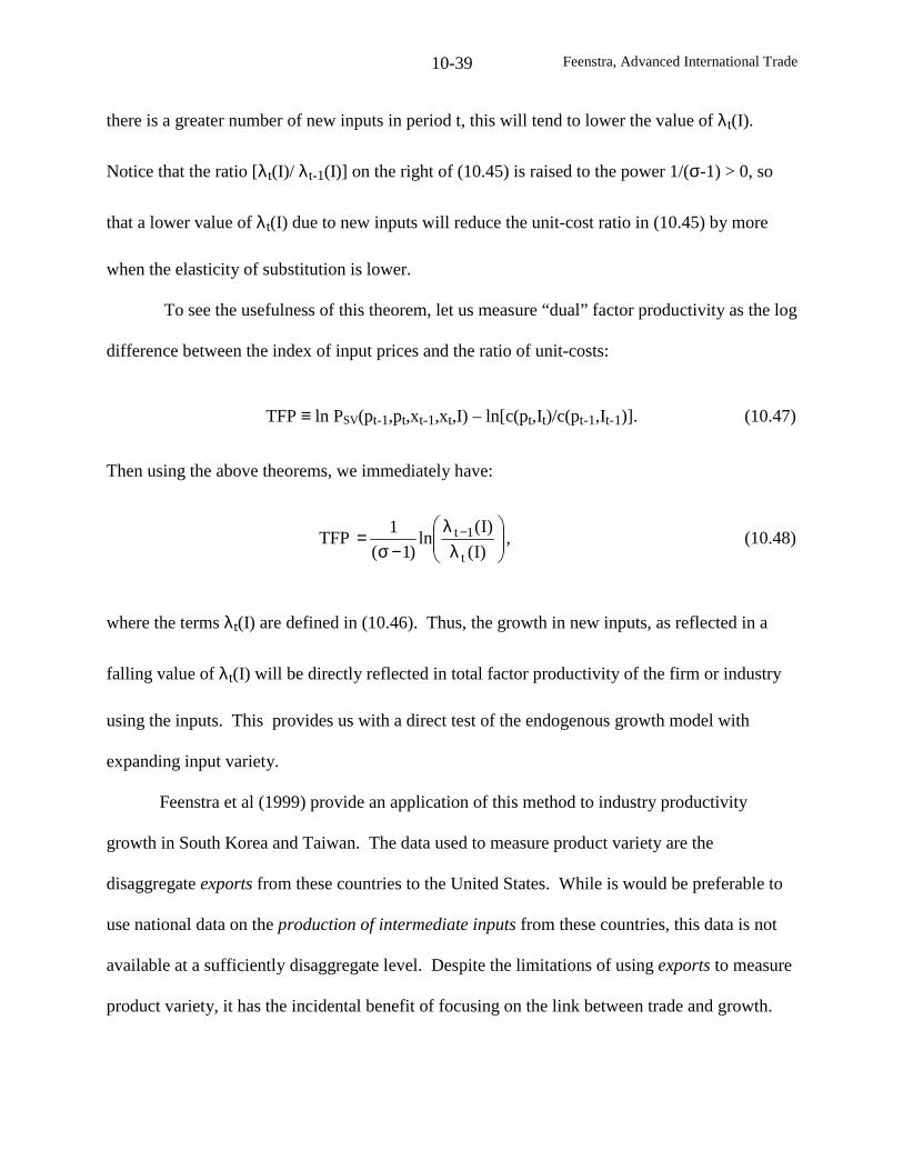
Feenstra, Advanced International Trade10-39
there is a greater number of new inputs in period t, this will tend to lower the value of λt(I).
Notice that the ratio [λt(I)/ λt-1(I)] on the right of (10.45) is raised to the power 1/(σ-1) > 0, so
that a lower value of λt(I) due to new inputs will reduce the unit-cost ratio in (10.45) by more
when the elasticity of substitution is lower.
To see the usefulness of this theorem, let us measure “dual” factor productivity as the log
difference between the index of input prices and the ratio of unit-costs:
TFP ≡ ln PSV(pt-1,pt,xt-1,xt,I) – ln[c(pt,It)/c(pt-1,It-1)]. (10.47)
Then using the above theorems, we immediately have:
TFP
λ
λ−σ
= −)I(
)I(ln
)1(
1
t
1t , (10.48)
where the terms λt(I) are defined in (10.46). Thus, the growth in new inputs, as reflected in a
falling value of λt(I) will be directly reflected in total factor productivity of the firm or industry
using the inputs. This provides us with a direct test of the endogenous growth model with
expanding input variety.
Feenstra et al (1999) provide an application of this method to industry productivity
growth in South Korea and Taiwan. The data used to measure product variety are the
disaggregate exports from these countries to the United States. While is would be preferable to
use national data on the production of intermediate inputs from these countries, this data is not
available at a sufficiently disaggregate level. Despite the limitations of using exports to measure
product variety, it has the incidental benefit of focusing on the link between trade and growth.
Feenstra, Advanced International Trade10-40
These authors analyze the relationship between changes in export variety and the growth
in TFP across South Korea and Taiwan, in sixteen sectors over 1975-1991. The results lend
support to the endogenous growth model. They find that changes in relative export variety
(entered as either a lag or a lead) have a positive and significant effect on TFP in nine of the
sixteen sectors. Seven of the sectors are classified as secondary industries, in that they rely on as
well as produce differentiated manufactures, and therefore seem to fit the idea of endogenous
growth. Among the primary industries, which rely more heavily on natural resources, the
authors find mixed evidence: the correlation between export variety and productivity can be
positive, negative, or insignificant. In addition, the authors also find evidence of a positive and
significant correlation between upstream export variety and productivity in six sectors, five of
which are secondary industries.
Funke and Ruhwedel (2001) have applied the same measure of product variety to analyze
economic growth across the OECD countries. Using a panel dataset of 19 countries over 1989-
1996, they find that a country’s export variety relative to the U.S. is a significant determinant of
its GDP per-capita. Notice that these measures of product variety, which are constructed from
highly disaggregate trade data, are unlikely to suffer from the endogeneity problem that plagues
aggregate trade flows (as addressed by Frankel and Romer, 1999). Therefore, the construction of
product variety indexes and their correlation with TFP offers an alternative way to assess the
importance of trade in economic growth.
Conclusions
This chapter began with a discussion of productivity growth for a firm or industry. The
measure of total factor productivity (TFP) due to Solow (1957) is the growth of output minus a
weighted average of the growth of inputs. The weights equal the elasticity of output with respect
Feenstra, Advanced International Trade10-41
to the inputs. Under perfect competition and constant returns to scale, these weights are easily
measured by the revenue-shares of the inputs. Without these assumptions, however, the
measurement of productivity growth becomes more difficult. Using the techniques of Hall
(1988), we showed how “true” productivity growth can be identified, along with estimating the
price-cost margins and returns to scale in an industry. This technique has been applied by
Levinsohn (1993) and Harrison (1994) to measure the reduction in markups following
liberalization in Turkey and the Ivory Coast, respectively.
Dropping the assumptions of perfect competition and constant returns to scale is also the
starting point of the literature on endogenous growth. While there are several types of
endogenous growth models, the one we considered in this chapter relied on expanding varieties
of intermediate inputs. An essential assumption was that the fixed cost of inventing a new input
is inversely proportional to the number of inputs already created. In the case where free trade in
goods and inputs also brings international spillovers of knowledge, then trade leads to an
increase in the growth rates of both countries (Grossman and Helpman, 1990, 1991). But if there
are no knowledge spillovers across borders, then free trade in goods has the effect of slowing
down product development in the smaller country, which may also bring losses due to trade
(Feenstra, 1996). This leads to several important empirical questions: (i) does free trade increase
growth rates; (ii) are knowledge spillovers global or local; (iii) is there any direct evidence on the
link between product variety and productivity? There is recent empirical work on all these
questions, but still some unanswered questions.
In particular, it seems that the differences in per-capita GDP across countries, which are
as large as ever, must be due to technology differences across countries (Easterly and Levine,
2000). This brings us right back to chapter 2, where we found that the HO model can account
Feenstra, Advanced International Trade10-42
for trade patterns only if it is extended to incorporate such technology differences. What is the
source of these? The endogenous growth model in this chapter has economy-wide increasing
returns to scale, whereby larger countries create more inputs and are thereby more productive. It
seems to me that we have not yet related this potential explanation for country productivity
differences to the implied productivity differences arising from the HO model. Could it be the
case that large countries (measured inclusive of proximity to neighbors) are the most productive
due to their input variety, and that this productivity also accounts for their trade patterns?
Addressing this question is one area for further research.
Feenstra, Advanced International Trade10-43
Problems
10.1 In the two-good, two-factor model with constant prices, suppose that good 1 experiences
Hicks-neutral technological progress, i.e. y1= A1f1(L1,K1), with A1 rising. Also assume that
good 1 is labor intensive. Then write down the zero-profit and full-employment conditions for
the economy, and use the Jone’s algebra to show the following:
(a) r0Aw 1 >>>
(b) 211 y0Ay >>>
Note: Part (b) is rather tricky, so you may not get all of it. If you understand why it is tricky,
that is good enough.
10.2 Let us adopt a translog functional form for the GDP function in (10.12), extended to
include many outputs:
.Vln)pAln(VlnVln
)pAln()pAln(Vln)pAln(Gln
k
N
1i
M
1kiiik
M
1k
M
1kk2
1
jj
N
1i
N
1jiiij
N
1i
M
1k2
1kkiii0
∑∑∑∑
∑∑∑ ∑
= == =
= == =
φ+δ+
γ+β+α+α=
ll
l
Differentiating this with respect to ipln , we obtain the output share equations,
k
M
1kik
N
1jjjijii Vln)pAln(s ∑∑
==φ+γ+α= , i=1,…,N.
where si = piyi/G is the share of each output in GDP.
(a) Write the quantity of each output as )p/Gsln(yln iii = . Differentiate this with respect to
ipln and obtain an expression for the output elasticity )pln/yln( ii ∂∂ . What restriction on the
translog parameters must hold for this elasticity to be positive?
Feenstra, Advanced International Trade10-44
(b) Write the quantity of each output as )p/Gsln(yln iii = . Differentiate this with respect to
iAln and obtain an expression for the “Rybczynski-like” elasticity )Aln/yln( ii ∂∂ . If the
restrictions in (a) are satisfied, then what can we say about the magnitude of this elasticity?
10.3 Consider the problem of maximizing (10.18) subject to (10.19), where for convenience we
set t = 0. Write this as the Lagrangian,
∫∞ ρτ− ττ−τ0
d)](Pln)(E[lne + }{0
)(R0
)(R d)(Ee)t(ALd)(we ∫∫∞ τ−∞ τ− ττ−+ττλ
= ∫∞ ρτ− ττ−τ
td)](Pln)(E[lne{ + )t(Bd)](EL)(w[e })(R λ+ττ−τλτ− ,
where in the second line we bring the Lagrange multiplier inside the integral. The expression
inside the integral must be maximized at every point in time. So differentiate this expression
with respect to E(τ) to obtain the first-order condition (10.20).
10.4 Consider a central planner who chooses the time-path of output to maximize utility. This
problem can be written as,
∫∞ −τρ−
τττ
t)t(
)(Yd)(Ylnemax ,
subject to,
XNxNY )1/(1)1/( −σ−σσ == and L = X + )N/N( &α ,
where X ≡ Nx and the constraints are the production function (10.17) along with the full-
employment condition (10.26). Let us restrict our attention to steady-state solutions
where )t(ge)t(N)(N −τ=τ . Substituting this equation along with the constraints into the
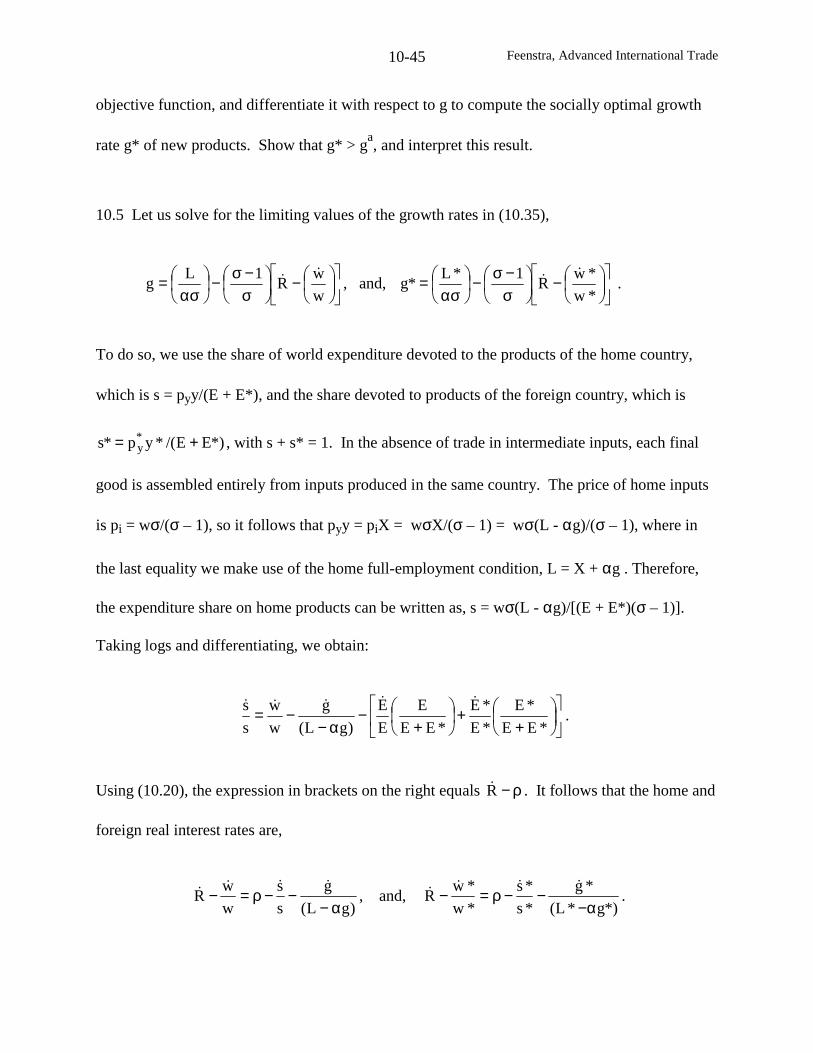
Feenstra, Advanced International Trade10-45
objective function, and differentiate it with respect to g to compute the socially optimal growth
rate g* of new products. Show that g* > ga, and interpret this result.
10.5 Let us solve for the limiting values of the growth rates in (10.35),
−
σ−σ−
ασ=
w
wR
1Lg
&& , and,
−
σ−σ−
ασ=
*w
*wR
1*L*g
&& .
To do so, we use the share of world expenditure devoted to the products of the home country,
which is s = pyy/(E + E*), and the share devoted to products of the foreign country, which is
*)EE/(*yp*s *y += , with s + s* = 1. In the absence of trade in intermediate inputs, each final
good is assembled entirely from inputs produced in the same country. The price of home inputs
is pi = wσ/(σ – 1), so it follows that pyy = piX = wσX/(σ – 1) = wσ(L - αg)/(σ – 1), where in
the last equality we make use of the home full-employment condition, L = X + αg . Therefore,
the expenditure share on home products can be written as, s = wσ(L - αg)/[(E + E*)(σ – 1)].
Taking logs and differentiating, we obtain:
++
+−
α−−=
*EE
*E
*E
*E
*EE
E
E
E
)gL(
g
w
w
s
s &&&&&.
Using (10.20), the expression in brackets on the right equals ρ−R& . It follows that the home and
foreign real interest rates are,
)gL(
g
s
s
w
wR
α−−−ρ=−
&&&& , and,*)g*L(
*g
*s
*s
*w
*wR
α−−−ρ=−
&&&& .
Feenstra, Advanced International Trade10-46
(a) The fact that the home country is developing more products than abroad means that
1st
lim =∞→
. What does this imply about the limiting value of the home real interest rate?
Therefore, what is the limiting value of the home growth rate?
(b) Since 1st
lim =∞→
, then 0*st
lim =∞→
. What can we say about the limiting values of the foreign
real interest rate, and the foreign growth rate?
Feenstra, Advanced International Trade
Chapter 11: Multinationals and Organization of the Firm
Despite the fact that this book is about international trade, we have so far not introduced
any role for traders. There has been little scope for firms, let alone economic organization more
generally, to have any significant influence on trade patterns between countries. This contradicts
the empirical fact that a good deal of trade occurs internally within firms located across
countries. For the U.S., for example, about one-third of exports and over 40% of imports consist
of intra-firm trade between a U.S. or foreign firm and their affiliates – see Table 11.1. When a
firm operates in several countries it is a multinational enterprise, and the investment made in the
foreign country is referred to as foreign direct investment (FDI).1 The first goal of this chapter is
to introduce these features into our earlier trade models.
The classic treatment of a multinational is that it has some intangible asset (such as
knowledge of a production process) that it can use to its advantage in a foreign market. It must
decide whether to simply export there, or to invest in that market by building a plant and selling
the product, or whether to engage in a joint venture or other contractual arrangement with a
foreign firm to produce the good. We will initially focus on the first two decisions – whether to
export to the foreign market or to build a plant and sell there. The third case – whether to engage
in a joint venture with a foreign firm –will be discussed at the end of the chapter. Notice that this
classic statement of the problem can equally well work in reverse, whereby the acquisition of a
foreign firm can bring with it some knowledge of value to the purchaser, that could not be
obtained by simply buying the products of that foreign firm.2
1 We might define FDI as acquiring sufficient assets in a foreign firm to exercise some managerial control, thoughacquiring 10% or more of the assets of a foreign enterprise is the definition commonly used in practice.2 Blonigen (1997) argues that increased inflows of Japanese acquisition FDI into the U.S. during 1985-1990 weremotivated by the desire to acquire the knowledge assets of U.S. firms, combined with the low value of the dollar.Notice that by this argument, FDI flows depend on the level of exchange rates.
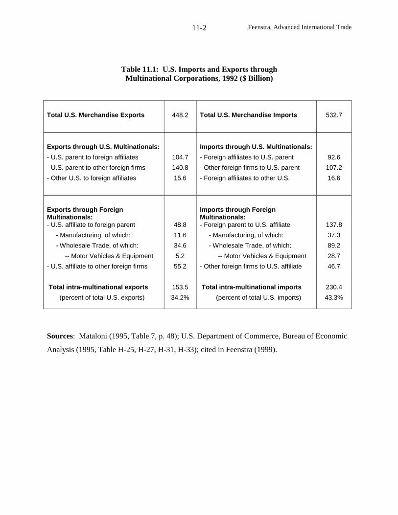
Feenstra, Advanced International Trade11-2
Table 11.1: U.S. Imports and Exports throughMultinational Corporations, 1992 ($ Billion)
Total U.S. Merchandise Exports 448.2 Total U.S. Merchandise Imports 532.7
Exports through U.S. Multinationals: Imports through U.S. Multinationals:
- U.S. parent to foreign affiliates 104.7 - Foreign affiliates to U.S. parent 92.6
- U.S. parent to other foreign firms 140.8 - Other foreign firms to U.S. parent 107.2
- Other U.S. to foreign affiliates 15.6 - Foreign affiliates to other U.S. 16.6
Exports through ForeignMultinationals:
Imports through ForeignMultinationals:
- U.S. affiliate to foreign parent 48.8 - Foreign parent to U.S. affiliate 137.8
- Manufacturing, of which: 11.6 - Manufacturing, of which: 37.3
- Wholesale Trade, of which: 34.6 - Wholesale Trade, of which: 89.2
-- Motor Vehicles & Equipment 5.2 -- Motor Vehicles & Equipment 28.7
- U.S. affiliate to other foreign firms 55.2 - Other foreign firms to U.S. affiliate 46.7
Total intra-multinational exports 153.5 Total intra-multinational imports 230.4
(percent of total U.S. exports) 34.2% (percent of total U.S. imports) 43.3%
Sources: Mataloni (1995, Table 7, p. 48); U.S. Department of Commerce, Bureau of Economic
Analysis (1995, Table H-25, H-27, H-31, H-33); cited in Feenstra (1999).
Feenstra, Advanced International Trade11-3
We see that the decision to engage in FDI by a multinational therefore involves three
interrelated aspects – ownership of an asset, location to produce, and whether to keep the asset
internal to the firm – and these comprise the so-called “OLI framework” of multinational activity
(Dunning, 1977, 1981). In the following sections, we explore models giving insight into these
various aspects. We begin with the simplest example where a firm considers shutting down its
factory in one country and moving it to another, which can be modeled by a movement of
physical capital across countries. While such a movement of capital does not necessarily occur
with FDI (which may simply involve a change in ownership without any movement of physical
capital), it is a useful place to begin our analysis.
After briefly reviewing capital inflows into a one-sector economy, we use the classic
article by Mundell (1957) to investigate capital mobility in the two-sector Heckscher-Ohlin (HO)
model. In that case we find that even small tariffs have a very large impact on the movement of
capital from one country to the other. This phenomenon of “tariff-jumping” FDI is a typical
occurrence in import-substitution regimes, but is not restricted to the developing countries:
many industrialized countries have used tariffs or quotas to induce the entry of foreign firms.
This policy has some economic rationale, since the entry of foreign firms in simple models leads
to a welfare gain due to increased domestic wages. The link between foreign investment and
wages is therefore an important topic for empirical research. In Mundell’s analysis, domestic
wages are not affected by the foreign investment (due to “factor price insensitivity” in the HO
model), but it is still the case that the deadweight loss of the tariff is reduced due to the entry of
foreign firms.
Multinationals need not lead to capital flows between countries, however, and may
instead just involve the ownership and location of firms. We consider several models of that
Feenstra, Advanced International Trade11-4
type, distinguishing vertical from horizontal multinationals. An example of the former case is a
firm that has headquarters in one country but does production in another to obtain lower factor
prices there (Helpman, 1984). The latter case occurs when a firm decides to duplicate
production facilities and sell locally in two or more countries, due to tariffs or other barriers
between them (Markusen, 1984, 2002). We identify conditions under which a particular type of
multinational is most likely to arise in equilibrium, and once again, find that trade policies can
have a significant impact on multinational location.
Beyond trade that is internal to multinational firms, there is another large portion of trade
that occurs between firms that have some special relationship. An example is when a firm
outsources some of its production process to a lower-wage country. In chapter 4 we modeled
this as the purchase of intermediate inputs, but in fact, it often involves a longer-term
relationship: the firm wanting to purchase the input is committing its money, and the selling
firm is committing resources to production and development of the inputs. This relationship
entails risk to both parties, and in many circumstances these risks cannot be offset by legal
contracts. If the costs associated with these incomplete contracts are too great, then the firm
wanting to purchase the inputs will instead vertically-integrate into this activity, becoming a
vertical multinational. Thus, a consideration of transactions costs under incomplete contracts
allows us to model the internalization decision of a multinational firm. The recent work of
Grossman and Helpman (2002a,b) and others puts this in a general equilibrium setting, and
investigates the implications of internalization for trade.
Transactions costs is the first and foremost reason for firms to integrate, but there are
others. For example, joint ventures between firms in different countries can bring with them
knowledge of the supplier and distribution networks in each country, and any other intangible
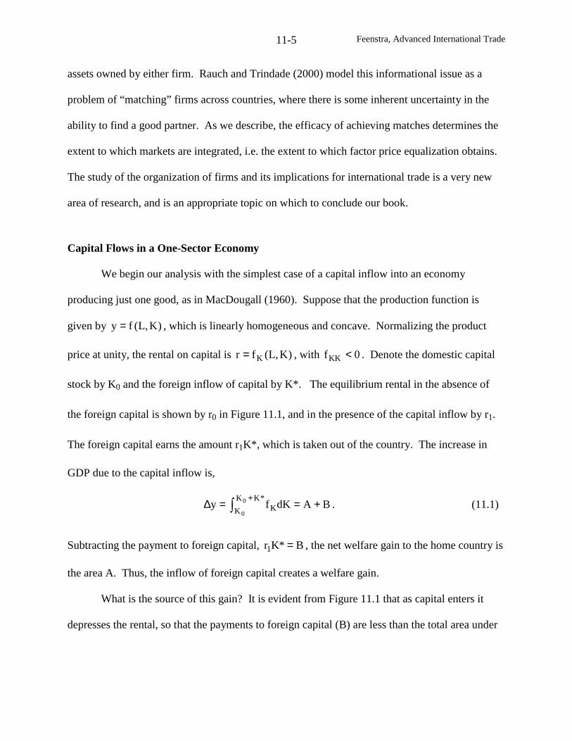
Feenstra, Advanced International Trade11-5
assets owned by either firm. Rauch and Trindade (2000) model this informational issue as a
problem of “matching” firms across countries, where there is some inherent uncertainty in the
ability to find a good partner. As we describe, the efficacy of achieving matches determines the
extent to which markets are integrated, i.e. the extent to which factor price equalization obtains.
The study of the organization of firms and its implications for international trade is a very new
area of research, and is an appropriate topic on which to conclude our book.
Capital Flows in a One-Sector Economy
We begin our analysis with the simplest case of a capital inflow into an economy
producing just one good, as in MacDougall (1960). Suppose that the production function is
given by )K,L(fy = , which is linearly homogeneous and concave. Normalizing the product
price at unity, the rental on capital is )K,L(fr K= , with 0fKK < . Denote the domestic capital
stock by K0 and the foreign inflow of capital by K*. The equilibrium rental in the absence of
the foreign capital is shown by r0 in Figure 11.1, and in the presence of the capital inflow by r1.
The foreign capital earns the amount r1K*, which is taken out of the country. The increase in
GDP due to the capital inflow is,
BAdKfy*KK
K K0
0+==∆ ∫
+. (11.1)
Subtracting the payment to foreign capital, B*Kr1 = , the net welfare gain to the home country is
the area A. Thus, the inflow of foreign capital creates a welfare gain.
What is the source of this gain? It is evident from Figure 11.1 that as capital enters it
depresses the rental, so that the payments to foreign capital (B) are less than the total area under
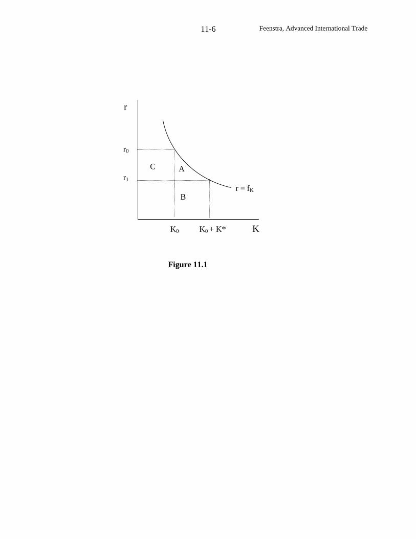
Feenstra, Advanced International Trade11-6
Figure 11.1
K0 K0 + K* K
A
r
r0
r1
Br = fK
C
Feenstra, Advanced International Trade11-7
the demand curve (A+B). The other side of this is that the capital inflow raises the marginal
product of labor and wages w = fL(L,K). Indeed, the total increase in the wage bill equals the
area A+C in Figure 11.1.3 Area C is the redistribution of income from capital to labor, whereas
area A is the net welfare gain and it accrues to labor.
These simple observations have led to a good deal of empirical work as to whether
industries experiencing an inflow of foreign capital pay higher wages. For the U.S., Howenstein
and Zeile (1994) and Doms and Jensen (1996) find that foreign plants pay higher wages than
domestic plants. Blonigen and Tomlin (1999) further find that foreign plants typically grow
faster than U.S. plants of similar size, and that they lead to a larger positive impact on local
wages than does domestic investment. Combining U.S. data with information on Mexican and
Venezuelan enterprises, Aitken et al (1996) also find a wage differential between domestic and
foreign-owned enterprises, even after controlling for industry size and capital-intensity.
Notice that these studies are most often comparing the wages paid by foreign versus
domestic plants, which is not exactly the same as the general equilibrium wage increase due to
foreign investment predicted by Figure 11.1. For example, if foreign firms simply attract the
highest-quality workers, this would lead to a wage increase over domestic plants, but not
necessarily welfare gains. This same problem of self-selection occurs in empirical studies of
technology transfer between foreign and local firms (through joint ventures or other spillovers
across firms). Evidence in support of technology transfer for Mexico is found by Blomstrom
(1986), Blomstrom and Persson (1983), and Kokko (1994), and for Indonesia by Blomstrom and
Sjoholm (1999). These studies correlate industry productivity with the presence of foreign
3 Because the production function is linearly homogeneous, then y0 = w0L + r0K0, and y1 = w1L + r1(K0 + K*). It
follows that *KrK)rr(L)ww()BA(y 100101 +−+−=+=∆ , and since *KrB 1= and 010 K)rr(C −= , then the
wage bill changes by .CA*KrK)rr()BA(L)ww( 100101 +=−−−+=−
Feenstra, Advanced International Trade11-8
firms. However, this leaves open the question of whether the higher productivity is due to the
foreign plants themselves, or due to spillovers. This has been addressed using plant level data by
Haddad and Harrison (1993) for Morocco, and Aitken and Harrison (1999) for Venezuela. They
find that the foreign plants indeed have higher productivity, but that there is a weak negative
correlation between their presence and productivity of the domestic plants in the same industry.
Thus, these finding cast some doubt on the hypothesis of positive technological spillovers
between foreign and domestic firms; rather, foreign firms are just more productive.
Capital Flows in the Two-Sector Heckscher-Ohlin Model
We turn next to a famous example of capital flows in the two-sector HO model, due to
Mundell (1957). Suppose there are two countries with identical technologies and homothetic
tastes, initially engaged in free trade. With countries producing both goods and no factor
intensity reversals, the rental on capital is uniquely determined by the goods prices, which we
write as r(p1,p2) for both countries. In Figure 11.2 the endowment of the two countries is shown
at the point Vi, which we assume is inside the factor price equalization set so the rental on capital
is the same across countries.4 With free trade in goods, consumption of the two countries is
proportional and occurs along the diagonal of Figure 11.2, such as the point ADi(where D
iis the
consumption vector of each country, and multiplying by the technology matrix A converts this to
the factors embodied in consumption). In the case we have illustrated, country 1 is labor
abundant, and the move from Vito AD
iinvolves country 1 importing the capital-intensive good.
Assume that good 1 is capital intensive, so that 0p/)p,p(r 121 >∂∂ .
4 Refer the chapter 2, Figure 2.3, to review how this figure is constructed.
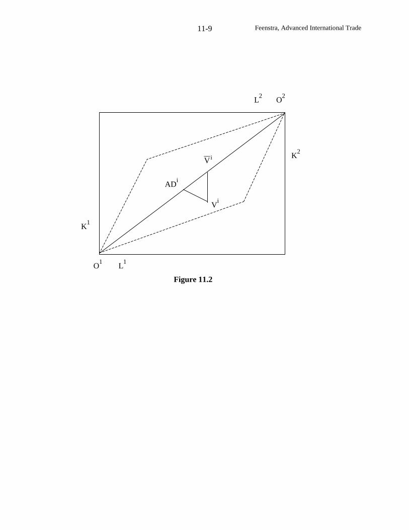
Feenstra, Advanced International Trade11-9
ADi
Vi
O1
L1
K1
K2
L2
O2
Figure 11.2
iV
Feenstra, Advanced International Trade11-10
Now allow for capital mobility between the countries, and suppose that country 1 applies
a specific import tariff of t > 0. This raises the domestic price of good 1 in that country, and
since this good is capital-intensive, by the Stolper-Samuelson theorem it increases the return to
capital, r(p1+t, p2) > r(p1, p2) . It follows that capital will flow from country 2 to country 1. In
Figure 11.2, this shifts the effective endowment point vertically upwards from point Vi. The
question is, where will this process end? The new equilibrium allowing for capital mobility
requires that the return to capital be equalized across the countries. But with the tariff driving a
wedge between the prices in the two countries, it is impossible for rentals to be equalized: t > 0
always implies that r(p1+t,p2) > r(p1,p2). Obviously, something in this equation must change to
achieve a new long-run equilibrium!
To see what changes, let us think about what happens as the endowments of the countries
move upwards from point Vi. Capital is flowing towards country 1, which increases the output
of industry 1 and reduces that of industry 2. Since good 1 is imported, the increased supply of
that good lowers imports, and the reduced supply of good 2 also lowers exports. So as we move
upwards from point Vi, trade between the countries is being reduced. This will continue until the
endowments reach the diagonal, indicated by the point iV , at which point the capital/labor ratios
in the two countries are identical. This means that there is no reason for trade: both economies
are in autarky.
What about the rental on capital in each country? Since both countries are in autarky,
with identical capital/labor ratios and identical homothetic tastes, this means that the equilibrium
prices are the same across countries. It follows therefore, that the equilibrium rental on capital is
also the same across countries. The tariff that is being applied by country 1 is redundant: since
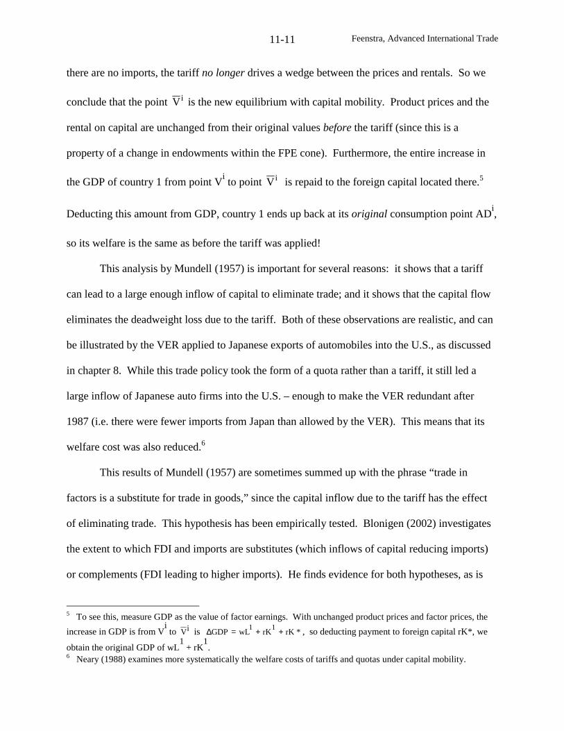
Feenstra, Advanced International Trade11-11
there are no imports, the tariff no longer drives a wedge between the prices and rentals. So we
conclude that the point iV is the new equilibrium with capital mobility. Product prices and the
rental on capital are unchanged from their original values before the tariff (since this is a
property of a change in endowments within the FPE cone). Furthermore, the entire increase in
the GDP of country 1 from point Vito point iV is repaid to the foreign capital located there.5
Deducting this amount from GDP, country 1 ends up back at its original consumption point ADi,
so its welfare is the same as before the tariff was applied!
This analysis by Mundell (1957) is important for several reasons: it shows that a tariff
can lead to a large enough inflow of capital to eliminate trade; and it shows that the capital flow
eliminates the deadweight loss due to the tariff. Both of these observations are realistic, and can
be illustrated by the VER applied to Japanese exports of automobiles into the U.S., as discussed
in chapter 8. While this trade policy took the form of a quota rather than a tariff, it still led a
large inflow of Japanese auto firms into the U.S. – enough to make the VER redundant after
1987 (i.e. there were fewer imports from Japan than allowed by the VER). This means that its
welfare cost was also reduced.6
This results of Mundell (1957) are sometimes summed up with the phrase “trade in
factors is a substitute for trade in goods,” since the capital inflow due to the tariff has the effect
of eliminating trade. This hypothesis has been empirically tested. Blonigen (2002) investigates
the extent to which FDI and imports are substitutes (which inflows of capital reducing imports)
or complements (FDI leading to higher imports). He finds evidence for both hypotheses, as is
5 To see this, measure GDP as the value of factor earnings. With unchanged product prices and factor prices, the
increase in GDP is from Vi
to iV is *rKrKwLGDP11 ++=∆ , so deducting payment to foreign capital rK*, we
obtain the original GDP of wL1
+ rK1.
6 Neary (1988) examines more systematically the welfare costs of tariffs and quotas under capital mobility.
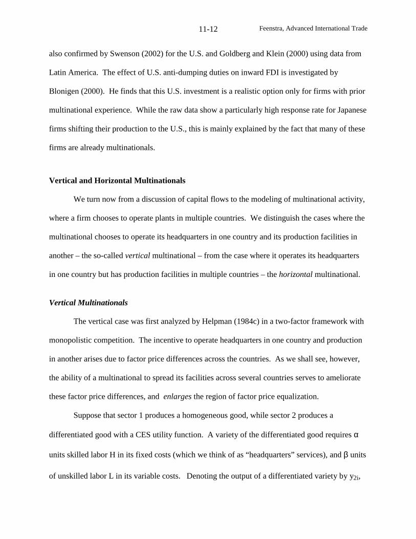
Feenstra, Advanced International Trade11-12
also confirmed by Swenson (2002) for the U.S. and Goldberg and Klein (2000) using data from
Latin America. The effect of U.S. anti-dumping duties on inward FDI is investigated by
Blonigen (2000). He finds that this U.S. investment is a realistic option only for firms with prior
multinational experience. While the raw data show a particularly high response rate for Japanese
firms shifting their production to the U.S., this is mainly explained by the fact that many of these
firms are already multinationals.
Vertical and Horizontal Multinationals
We turn now from a discussion of capital flows to the modeling of multinational activity,
where a firm chooses to operate plants in multiple countries. We distinguish the cases where the
multinational chooses to operate its headquarters in one country and its production facilities in
another – the so-called vertical multinational – from the case where it operates its headquarters
in one country but has production facilities in multiple countries – the horizontal multinational.
Vertical Multinationals
The vertical case was first analyzed by Helpman (1984c) in a two-factor framework with
monopolistic competition. The incentive to operate headquarters in one country and production
in another arises due to factor price differences across the countries. As we shall see, however,
the ability of a multinational to spread its facilities across several countries serves to ameliorate
these factor price differences, and enlarges the region of factor price equalization.
Suppose that sector 1 produces a homogeneous good, while sector 2 produces a
differentiated good with a CES utility function. A variety of the differentiated good requires α
units skilled labor H in its fixed costs (which we think of as “headquarters” services), and β units
of unskilled labor L in its variable costs. Denoting the output of a differentiated variety by y2i,
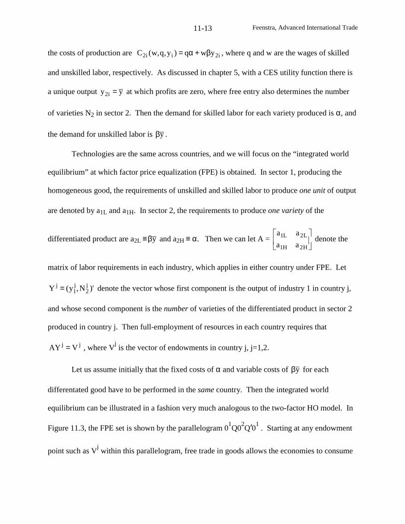
Feenstra, Advanced International Trade11-13
the costs of production are i2ii2 ywq)y,q,w(C β+α= , where q and w are the wages of skilled
and unskilled labor, respectively. As discussed in chapter 5, with a CES utility function there is
a unique output yy i2 = at which profits are zero, where free entry also determines the number
of varieties N2 in sector 2. Then the demand for skilled labor for each variety produced is α, and
the demand for unskilled labor is yβ .
Technologies are the same across countries, and we will focus on the “integrated world
equilibrium” at which factor price equalization (FPE) is obtained. In sector 1, producing the
homogeneous good, the requirements of unskilled and skilled labor to produce one unit of output
are denoted by a1L and a1H. In sector 2, the requirements to produce one variety of the
differentiated product are a2L ≡ yβ and a2H ≡ α. Then we can let A =
H2H1
L2L1
aa
aadenote the
matrix of labor requirements in each industry, which applies in either country under FPE. Let
)'N,y(Y j2
j1
j = denote the vector whose first component is the output of industry 1 in country j,
and whose second component is the number of varieties of the differentiated product in sector 2
produced in country j. Then full-employment of resources in each country requires that
jj VAY = , where Vjis the vector of endowments in country j, j=1,2.
Let us assume initially that the fixed costs of α and variable costs of yβ for each
differentated good have to be performed in the same country. Then the integrated world
equilibrium can be illustrated in a fashion very much analogous to the two-factor HO model. In
Figure 11.3, the FPE set is shown by the parallelogram 01Q0
2Q’01
. Starting at any endowment
point such as Vjwithin this parallelogram, free trade in goods allows the economies to consume
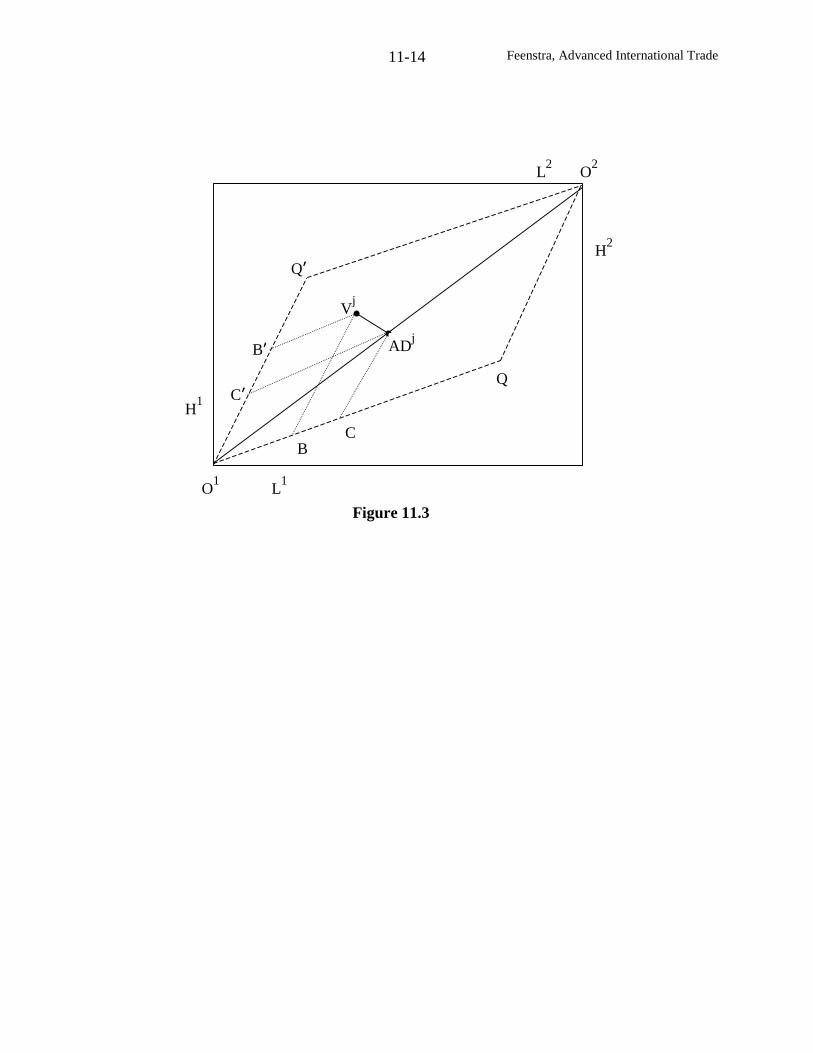
Feenstra, Advanced International Trade11-14
Figure 11.3
Vj
Q’
C
O1
L1
H1
H2
L2
O2
Q
B
ADj
B’
C’
Feenstra, Advanced International Trade11-15
at points Djthat are proportional across countries, so that the factors embodied in consumption
ADjlie along the diagonal of the box.7 The slope of the line between V
jand AD
j(in absolute
value) is the equilibrium ratio of factor prices w/q.
Let us assume that industry 1, producing the homogeneous product, is unskilled-labor
intensive, so that a1L/a1H > a2L/a2H = yβ /α. Then from the endowment and consumption points
we can readily compute the trade balance in each industry. Thus, from the endowment point Vj,
country 1 uses the amount of unskilled labor 01B in industry 1, and 0
1B’ in industry 2. Similarly,
from the consumption point ADj, country 1 uses the amount of unskilled labor 0
1C in industry 1,
and 01C’ in industry 2. It follows that country 1 is an importer of good 1 (OB < OC), and a net
exporter of the differentiated good (OB’ > OC’). In addition, there is intra-industry trade in the
differentiated goods sector.
Now let us change our assumptions and suppose that the fixed costs of α skilled labor
and variable costs of yβ unskilled labor for each differentated good can be be performed in
different countries by a multinational firm. Then how does the ability to “fragment” the
headquarters and production activities across countries affect the FPE set? A quick (and entirely
correct) answer can be obtained by appealing to the FPE set with multiple goods developed by
Dixit and Norman (1980), as discussed in chapter 3. Rank the activities beginning with the
variable costs of producing the differentiated good, which uses only unskilled labor; followed by
the production of the homogeneous product which uses both factors; followed by the fixed costs
7 Note that the consumption in each country equals ]'s)NN(,d[D j22
12
j1
j += , where the first component is the
quantity consumed in country j of the homogeneous good, and the second component is the world variety of thedifferentiated good times country j’s share of world GDP.
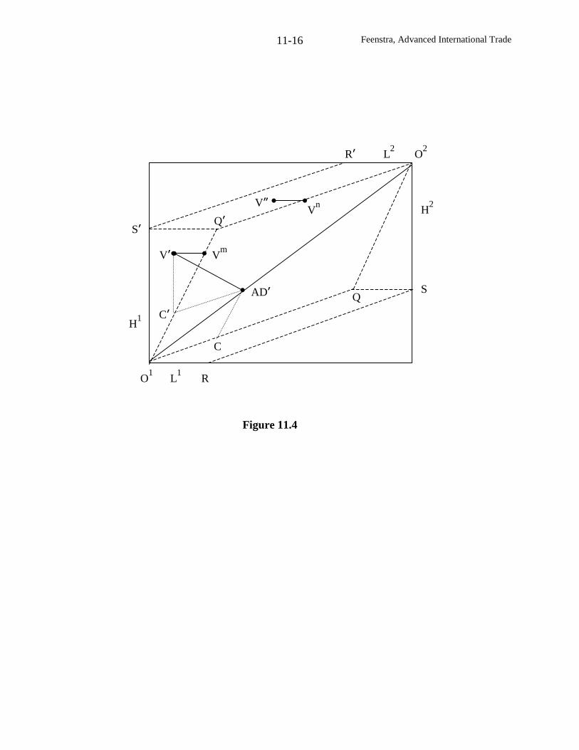
Feenstra, Advanced International Trade11-16
Q’
O1
L1
R
S’
H1
H2
S
R’ L2
O2
Q
V’
Vn
C
Vm
V”
AD’
C’
Figure 11.4
Feenstra, Advanced International Trade11-17
of producing the differentiated good, which uses only skilled labor. This gives three rather than
two factor requirements vectors, which are ( yβ ,0), (a1L,a1H), and (0,α). Multiplying each of
these by the total worldwide amount of each activity in the integrated equilibrium, and summing
them, we will obtain the FPE set 01RS0
2R’ S’01
in Figure 11.4. This FPE region is clearly larger
than the original parallelogram 01Q0
2Q’01
.
To understand how FPE is achieved in this expanded set, suppose that the factor
endowments of the two countries are given by V’ in Figure 11.4. This point lies outside the
original FPE set, so that any firm in sector 1 would choose the country with lowest wage of
skilled labor for headquarters, and the country with lowest wage of unskilled labor for
production. Since country 1 is skilled-labor abundant, we can presume that it would have the
lower relative wage of skilled labor, and firms from either country would want to establish
headquarters there. This will increase the demand for skilled labor in country 1, to the point
where the entire endowment V’ can be employed at the same factor prices as prevailing abroad.
Intuitively, this is what allows FPE to hold in the expanded set.
Because there are three production activities and only two factors, there are actually
many combinations of the activities across countries that are consistent with full-employment
and FPE. As in Helpman (1984c), we will focus on those combinations that lead to a minimum
amount of trade. With factor endowments given by V’ in Figure 11.4, country 1 could produce
varieties of the differentiated good using resources shown by 01C’, and then devote its remaining
endowment of skilled labor, shown by C’V’, to headquarters services. These headquarters
services would be combined with unskilled labor in country 2, of the amount V’Vm, in order to
produce varieties of the differentiated product in that country. Additional resources in country 2,
Feenstra, Advanced International Trade11-18
of the amount Vm
Q’, would also be devoted to produce varieties of the differentiated product,
and the remaining resource of Q’02would be used to produce the homogeneous product in sector
1. Factor price equalization is achieved through combining skilled labor for headquarters
services in country 1 with unskilled labor for production in country 2.
What is the trade pattern implied by the multinational activity? For factor endowments in
the region 01S’ Q’, as we have been discussing, the homogeneous good is produced only in
country 2, so country 1 imports that good. But for the differentiated good, the trade pattern is not
so clear. Indeed, in the case we have illustrated in Figure 11.4, it turns out that both countries
have balanced net trade in the differentiated good. This can be seen by comparing the resources
used in production and consumption. As discussed just above, country 1 uses the resources 01C’
to produce varieties of the differentiated good. To determine its consumption, we can trace a line
from its endowment point V’ to its consumption of factors AD’ (this line has the slope w/q). We
then decompose the point AD’ into the consumption of factors 01C in sector 1, and 0
1C’ in sector
2. Notice that for the case we have illustrated, the consumption of factors 01C’ in sector 2 is
identical to those used in the production of differentiated varieties by country 1. It follows that
trade is balanced in that sector, and the same will hold for country 2: they have balanced intra-
industry trade in the differentiated good.8
How can country 1 be an importer of the homogeneous good, and yet have balanced net
trade in the differentiated good? The answer is that this country receives profits from its
8 It follows that for slightly different choices of the endowment point V’, country 1 could be either a net exporter or
a net importer of the differentiated good in the region 01S’ Q’.
Feenstra, Advanced International Trade11-19
multinationals engaged in production abroad, which would show up as investment income in the
current account. Thus, its balance of trade deficit (due to importing the homogeneous good) is
offset by receipts from its subsidiaries abroad, so that it has an overall current account balance.
The amount of profits earned in country 2 will be proportional to the unskilled labor employed
there by the multinationals, which is measured by L* ≡ V’Vm. With yβ units of unskilled labor
needed per variety, the number of varieties produced by multinationals in country 2 is therefore
N* ≡ L*/ yβ . The value of headquarters services provided by these multinationals through
employing skilled labor in country 1 is then αN* = αL*/ yβ .9 This is an “invisible export” by
country 1, which is used to pay for its imports of the homogeneous good.
As we move to other regions of the FPE set, the trade patterns change. For example,
consider endowment within 02R’ S’ Q’ , such as V”. Once again, multinationals with
headquarters in country 1 will use some of the unskilled labor in country 2 so that FPE is
achieved. In this case, the amount of unskilled labor employed in country 2 by multinationals is
the distance V”Vn. We can think of the vector 0
1V
nas the employment of resources by firms that
have headquarters in country 1, as distinct from that country’s endowment vector 01V”. In the
absence of multinationals, the employment of resources must equal a country’s endowment, but
now they can differ. We can also construct the trade patterns in the region 02R’ S’ Q’. It turns
out the country 1 can be either an importer or an exporter of the homogeneous product in this
region, and also exports the differentiated product as well as headquarters services.10
9 Notice that the skilled labor of αN* = αL*/ yβ in country 1 is equivalently measured by the distance C’V’.10 Helpman (1984c) carefully solves for the trade pattern in this region, as well as showing how endowments affectthe volume of trade in all regions of the FPE set.
Feenstra, Advanced International Trade11-20
Setting aside the details of the trade patterns, the most important message to take from
Figure 11.4 is that vertical multinationals enlarge the FPE set. This is a deep insight from
Helpman (1984c), and can be compared to our results in chapter 4, where we discussed trade in
intermediate inputs and wages. We suggested there that the ability to fragment the production
process, and purchase some unskilled-labor intermediate inputs from another country, could lead
to an increase in the relative demand and wages of skilled labor in both countries. In
comparison, we have argued above that such outsourcing by multinationals will lead to an
enlargement of the FPE set, and therefore, a tendency for factor prices to equalize across
countries. These two results are not necessarily inconsistent, but it is worth thinking about how
the assumptions of Helpman (1984c) differ from those in chapter 4.
In the model of chapter 4 with a continuum of inputs, we showed that an increase in
outsourcing would occur through the “borderline” activity being transferred from the home to the
foreign country: that activity was less skill-intensive than any other activity performed at home,
but more skill-intensive than any other activity performed abroad. Therefore, the relative
demand for skilled labor rose in both countries, as did its relative wage. In contrast, in our
discussion of Helpman’s (1984) model above, we treated the production of the differentiated
good as using only unskilled labor, with headquarters services using only skilled labor. The
production activity is therefore less skill-intensive than the homogeneous good produced in
either country. The transfer of multinational production from country 1 to country 2 raises the
relative demand for skilled labor in country 1, but lowers it in country 2. This will raise the
relative wages of skilled labor in country 1, but lower it in country 2, thereby moving these
relative wages towards equality, so that FPE is achieved.

Feenstra, Advanced International Trade11-21
We see that the assumptions on factor-intensities differ between chapter 4 and what we
have used to describe Helpman’s (1984) model.11 Obviously, other assumptions on factor-
intensities can be incorporated into Helpman’s model, as well as alternative assumptions on fixed
costs and trade barriers, as we shall explore in the next section.
Horizontal Multinationals
In Helpman’s model, the multinational will never choose to operate production facilities
in both countries, because with free trade, there is no benefit to doing so. But suppose that there
are some trade barriers, such as the “iceberg” transport costs discussed in chapter 5. Suppose
further that each plant has some specific fixed costs, which must be borne in the same country as
production costs. Then we will say that horizontal FDI occurs if a firm chooses to operate
production facilities in multiple countries, with each plant selling locally to that market.
Horizontal FDI requires that the gains from selling locally and thereby avoiding transport costs
more than offset the plant-specific fixed costs. This case has been analyzed in a series of papers
beginning with Markusen (1984) and culminating in the book by Markusen (2002). These
writings cover a whole range of vertical and horizontal multinationals, using unskilled and
skilled labor in varying proportions. We will not attempt to summarize all these results, but shall
develop one example of how horizontal multinationals can arise.
We suppose that a firm in country i is already producing for its home market, and is
deciding whether to export to county j or establish a production facility and sell there. This firm
has already covered its fixed costs of headquarters services, as well as any plant-specific fixed
11 Helpman (1984c) actually uses more general assumption on factor intensities, but to illustrate the FPE regions,focuses on the case where the fixed costs use only skilled labor (which he calls a “general purpose” input H), and thevariable costs use only unskilled labor. These are the same assumptions we have used above. In related theoreticalwork, Helpman (1985) allows for multinationals to produce multiple products.
Feenstra, Advanced International Trade11-22
costs in country i, and there is an additional fixed cost of establishing a plant abroad. We
suppose there are “iceberg” transportation costs between the countries, so that Tij
> 1 units of the
good must be exported from country i in order for one unit to arrive in j. We let pidenote the
f.o.b. price received by the firm in country i. Inclusive of the transportation costs, the c.i.f. price
abroad is pij
= Tij
pi.
We borrow the demand structure from our treatment of monopolistic competition in
chapter 5. With country j having a CES utility function over the differentiated product, its
demand cij
for a variety sent from country i is:
)P/(Y)/Pp(c jj-jijij σ= , (11.2)
Yjis country j’s GDP and P
jrefers to country j’s overall price index, defined as:
( ))(pNP)-11/(C
1i-1ijij σ
=σ∑= , (11.3)
where Niis the number of products exported by each country i=1,…,C.
We treat labor as the only factor of production, and do not distinguish by skill type. The
exporting firm in country i has the production function Li= βy
i, where β is its marginal labor
costs. Note that its plant-specific fixed costs are already covered by virtue of its home sales of
this product. Revenue received from producing in country i and exporting is pijc
ij= p
iy
i, where
output is related to consumption by yi= c
ijT
ij. The profits from exporting are then:
ijijiiiiii cT)wp(ywyp β−=β− . (11.4)
Feenstra, Advanced International Trade11-23
Substituting for the CES demand from (11.3), and maximizing (11.4) over the choice of the price
pij
= Tij
pi, we readily obtain the optimal price p
i[1–(1/σ)] = βw
i. Substituting this back into
(11.4), we obtain the maximized value of profits:
σ=β−
iiiiii yp
ywyp
σ=
σ
j
j-
j
ijiiji
P
Y
P
TpTp j1
j
iji
YP
Tp1σ−
σ= , (11.5)
where the second equality follows using consumption from (11.2) with yi= c
ijT
ij, and the third
by simplification. From (11.5), we see that higher transport costs reduce profits from exporting,
while higher GDP abroad increase profits.
Rather than exporting from country i, the multinational firm can instead establish a
production facility in country j, and sell locally. In that case, it will face the production function
Lj= αj
+ βyj, including the plant-specific fixed costs paid abroad. For simplicity we treat
marginal labor costs β as equal across countries, though the wages and fixed costs can differ.
There are no transport costs when producing in country j and selling locally, so with the price pj,
the quantity sold is,
)P/(Y)/Pp(c jj-jjj σ= . (11.2’)
Again, the optimal price is determined as pj[1–(1/σ)] = βw
j. Using this and (11.2’) to compute
profits earned from the subsidiary in country j, we obtain:
)y(wyp jjjjj α−β− jjj
j-1
j
j
wP
Y
P
p1 α−
σ=
σ
. (11.5’)
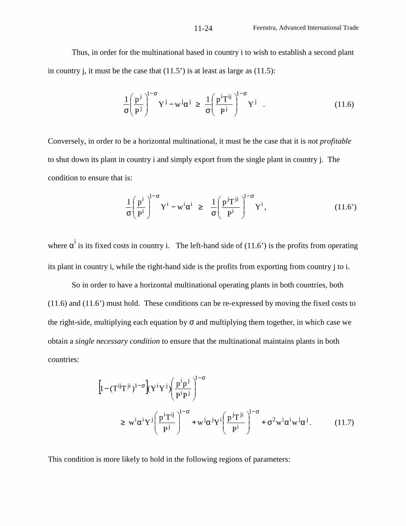
Feenstra, Advanced International Trade11-24
Thus, in order for the multinational based in country i to wish to establish a second plant
in country j, it must be the case that (11.5’) is at least as large as (11.5):
jjj1
j
j
wYP
p1 α−
σ
σ−j
1
j
iji
YP
Tp1σ−
σ≥ . (11.6)
Conversely, in order to be a horizontal multinational, it must be the case that it is not profitable
to shut down its plant in country i and simply export from the single plant in country j. The
condition to ensure that is:
iii1
i
i
wYP
p1 α−
σ
σ−i
1
i
jij
YP
Tp1σ−
σ≥ , (11.6’)
where αiis its fixed costs in country i. The left-hand side of (11.6’) is the profits from operating
its plant in country i, while the right-hand side is the profits from exporting from country j to i.
So in order to have a horizontal multinational operating plants in both countries, both
(11.6) and (11.6’) must hold. These conditions can be re-expressed by moving the fixed costs to
the right-side, multiplying each equation by σ and multiplying them together, in which case we
obtain a single necessary condition to ensure that the multinational maintains plants in both
countries:
[ ]σ−
σ−
−
1
ji
jiji1jiij
PP
pp)YY()TT(1
jjii21
i
jijijj
1
j
ijijii ww
P
TpYw
P
TpYw αασ+
α+
α≥
σ−σ−
. (11.7)
This condition is more likely to hold in the following regions of parameters:
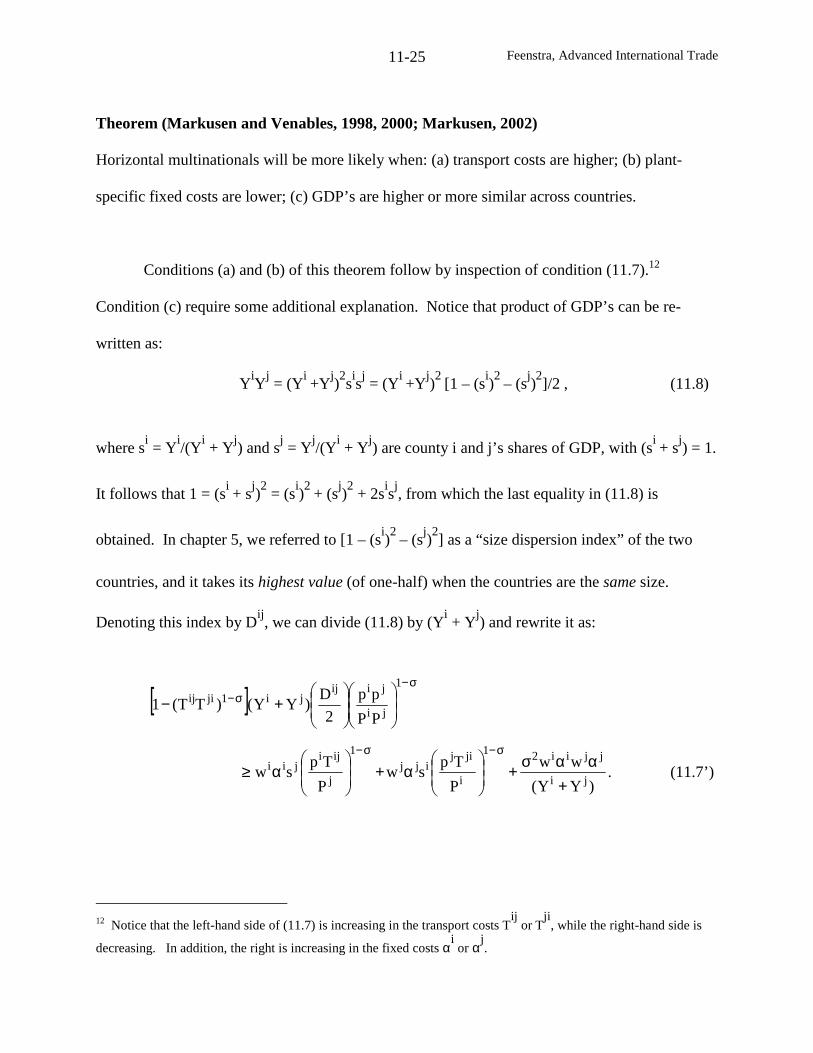
Feenstra, Advanced International Trade11-25
Theorem (Markusen and Venables, 1998, 2000; Markusen, 2002)
Horizontal multinationals will be more likely when: (a) transport costs are higher; (b) plant-
specific fixed costs are lower; (c) GDP’s are higher or more similar across countries.
Conditions (a) and (b) of this theorem follow by inspection of condition (11.7).12
Condition (c) require some additional explanation. Notice that product of GDP’s can be re-
written as:
YiY
j= (Y
i+Y
j)2sisj= (Y
i+Y
j)2
[1 – (si)2
– (sj)2]/2 , (11.8)
where si= Y
i/(Y
i+ Y
j) and s
j= Y
j/(Y
i+ Y
j) are county i and j’s shares of GDP, with (s
i+ s
j) = 1.
It follows that 1 = (si+ s
j)2
= (si)2
+ (sj)2
+ 2sisj, from which the last equality in (11.8) is
obtained. In chapter 5, we referred to [1 – (si)2
– (sj)2] as a “size dispersion index” of the two
countries, and it takes its highest value (of one-half) when the countries are the same size.
Denoting this index by Dij, we can divide (11.8) by (Y
i+ Y
j) and rewrite it as:
[ ]σ−
σ−
+−
1
ji
jiijji1jiij
PP
pp
2
D)YY()TT(1
)YY(
ww
P
Tpsw
P
Tpsw
ji
jjii21
i
jijijj
1
j
ijijii
+αασ+
α+
α≥
σ−σ−
. (11.7’)
12 Notice that the left-hand side of (11.7) is increasing in the transport costs Tij
or Tji
, while the right-hand side is
decreasing. In addition, the right is increasing in the fixed costs αi
or αj.
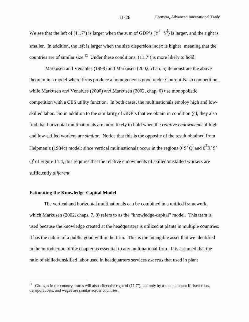
Feenstra, Advanced International Trade11-26
We see that the left of (11.7’) is larger when the sum of GDP’s (Yi+Y
j) is larger, and the right is
smaller. In addition, the left is larger when the size dispersion index is higher, meaning that the
countries are of similar size.13 Under these conditions, (11.7’) is more likely to hold.
Markusen and Venables (1998) and Markusen (2002, chap. 5) demonstrate the above
theorem in a model where firms produce a homogeneous good under Cournot-Nash competition,
while Markusen and Venables (2000) and Markusen (2002, chap. 6) use monopolistic
competition with a CES utility function. In both cases, the multinationals employ high and low-
skilled labor. So in addition to the similarity of GDP’s that we obtain in condition (c), they also
find that horizontal multinationals are more likely to hold when the relative endowments of high
and low-skilled workers are similar. Notice that this is the opposite of the result obtained from
Helpman’s (1984c) model: since vertical multinationals occur in the regions 01S’ Q’ and 0
2R’ S’
Q’ of Figure 11.4, this requires that the relative endowments of skilled/unskilled workers are
sufficiently different.
Estimating the Knowledge-Capital Model
The vertical and horizontal multinationals can be combined in a unified framework,
which Markusen (2002, chaps. 7, 8) refers to as the “knowledge-capital” model. This term is
used because the knowledge created at the headquarters is utilized at plants in multiple countries:
it has the nature of a public good within the firm. This is the intangible asset that we identified
in the introduction of the chapter as essential to any multinational firm. It is assumed that the
ratio of skilled/unskilled labor used in headquarters services exceeds that used in plant
13 Changes in the country shares will also affect the right of (11.7’), but only by a small amount if fixed costs,transport costs, and wages are similar across countries.

Feenstra, Advanced International Trade11-27
production by multinationals, which in turn exceeds that used in production of the homogeneous
competitive good. Then Markusen (2002, chap. 8) finds that increased investment by
multinationals raises the relative wage of skilled/unskilled workers in the skill-abundant country,
and possibly in the other country as well. The reason for this is that the skill-abundant country
specializes more in headquarters services, while the other country specializes more in production
by multinationals, which raise the relative demand for skilled labor in both countries. This
outcome applies to either horizontal or vertical investment, and is very similar to what we
obtained from outsourcing in chapter 4.14
The knowledge-capital model has been estimated by Carr, Markusen and Maskus (2001),
and hypothesis tests to distinguish the horizontal versus vertical model are performed by
Markusen and Maskus (1999, 2002) as well as Blonigen, Davies and Head (2002).15 These
papers differ somewhat in their precise specifications, and we will combine their various results
in our discussion below.16 The dependent variable used is the real sales of foreign affiliates of
multinational firms, including both their local and export sales. For horizontal multinationals the
local sales are most important, while for vertical multinational the export sales (back to the
parent corporation) are most important.
The equation estimated by Carr, Markusen and Maskus (2001) is:
14 Notice that the skilled/unskilled labor used in plant product in the knowledge capital model lies in-between thefactor intensities of headquarters services and of the homogeneous competitive good. This is similar to factorintensity of the “borderline” activity that was transferred between countries in the outsourcing model of chapter 4,but differs from the assumption of Helpman (1984c).15 Brainard (1997) also estimates a horizontal versus multinationals model in which firms trade-off the benefitsfrom being close to customers against the benefits of concentrating production in one location.16 In the estimation of (11.9), Blonigen, Davies and Head (2002) measure the skill difference and GDP differenceas absolute values instead. They argue that the absolute values are closer to the specification in Maskus andMarkusen (2002) and Markusen (2002, chap. 12), who allow for separate coefficients on the skill differencedepending on its sign, along with separate coefficients on its interaction with the GDP difference.
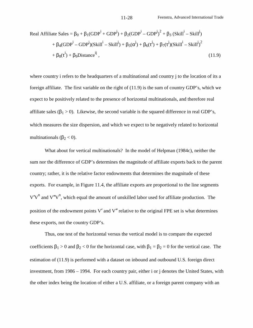
Feenstra, Advanced International Trade11-28
Real Affiliate Sales = β0 + β1(GDPi+ GDP
j) + β2(GDP
i– GDP
j)2
+ β3 (Skilli– Skill
j)
+ β4(GDPi– GDP
j)(Skill
i– Skill
j) + β5(αj
) + β6(τj) + β7(τj
)(Skilli– Skill
j)2
+ β8(τi) + β9Distance
ij, (11.9)
where country i refers to the headquarters of a multinational and country j to the location of its a
foreign affiliate. The first variable on the right of (11.9) is the sum of country GDP’s, which we
expect to be positively related to the presence of horizontal multinationals, and therefore real
affiliate sales (β1 > 0). Likewise, the second variable is the squared difference in real GDP’s,
which measures the size dispersion, and which we expect to be negatively related to horizontal
multinationals (β2 < 0).
What about for vertical multinationals? In the model of Helpman (1984c), neither the
sum nor the difference of GDP’s determines the magnitude of affiliate exports back to the parent
country; rather, it is the relative factor endowments that determines the magnitude of these
exports. For example, in Figure 11.4, the affiliate exports are proportional to the line segments
V’Vnand V”V
n, which equal the amount of unskilled labor used for affiliate production. The
position of the endowment points V’ and V” relative to the original FPE set is what determines
these exports, not the country GDP’s.
Thus, one test of the horizontal versus the vertical model is to compare the expected
coefficients β1 > 0 and β2 < 0 for the horizontal case, with β1 = β2 = 0 for the vertical case. The
estimation of (11.9) is performed with a dataset on inbound and outbound U.S. foreign direct
investment, from 1986 – 1994. For each country pair, either i or j denotes the United States, with
the other index being the location of either a U.S. affiliate, or a foreign parent company with an
Feenstra, Advanced International Trade11-29
affiliate in the U.S.. The hypotheses that β1 > 0 and β2 < 0 are strongly confirmed in the
estimation, which supports the horizontal over the vertical multinational model.
The next two variables in (11.9) are related to the skill differences between the parent and
host country, where Skilliis measured by the share of the labor force in certain skilled
occupations. In the horizontal model, it is expected that investment and affiliate sales are
declining in the endowment differences of the countries, and this effect is more pronounced
when the country GDP’s also differ. Thus, the hypotheses β3 < 0 and β4 < 0 are obtained from
the horizontal model. In contrast, with Helpman’s model vertical investment is higher when the
endowments of the countries differ more, so that β3 > 0 is predicted. Markusen (2002, chap. 12)
also finds in his simulations that countries that are both small and skilled-labor abundant relative
to their trading partners, such as the Netherlands, have the greatest concentration of headquarters
for vertical multinationals. Thus, the interaction between relative country size and the skill
endowment is positively related to vertical investment, so that β4 > 0 also.
In the estimation of (11.9), the sign pattern β3 < 0 and β4 < 0 is strongly confirmed, so
once again, the horizontal model is accepted and the vertical model is rejected. This outcome is
perhaps not surprising in view of the fact that the majority of foreign investments worldwide are
between industrial countries, and not between developed and developing countries (Markusen,
1995, and Lipsey, 1999, 2001). These investments would be more typical of horizontal rather
than vertical linkages. This tendency can be seen from the data on the stocks and flows of global
FDI over 1980-95, as shown in Tables 11.2 and 11.3.
Looking first at the inward stock of FDI in the upper-half of Table 11.2, the proportion of
FDI located in developing countries fluctuated between 19% and 26% over 1980-95, so the
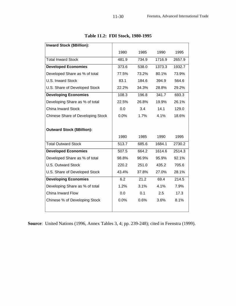
Feenstra, Advanced International Trade11-30
Table 11.2: FDI Stock, 1980-1995
Inward Stock ($Billion):
1980 1985 1990 1995
Total Inward Stock 481.9 734.9 1716.9 2657.9
Developed Economies 373.6 538.0 1373.3 1932.7
Developed Share as % of total 77.5% 73.2% 80.1% 73.9%
U.S. Inward Stock 83.1 184.6 394.9 564.6
U.S. Share of Developed Stock 22.2% 34.3% 28.8% 29.2%
Developing Economies 108.3 196.8 341.7 693.3
Developing Share as % of total 22.5% 26.8% 19.9% 26.1%
China Inward Stock 0.0 3.4 14.1 129.0
Chinese Share of Developing Stock 0.0% 1.7% 4.1% 18.6%
Outward Stock ($Billion):
1980 1985 1990 1995
Total Outward Stock 513.7 685.6 1684.1 2730.2
Developed Economies 507.5 664.2 1614.6 2514.3
Developed Share as % of total 98.8% 96.9% 95.9% 92.1%
U.S. Outward Stock 220.2 251.0 435.2 705.6
U.S. Share of Developed Stock 43.4% 37.8% 27.0% 28.1%
Developing Economies 6.2 21.2 69.4 214.5
Developing Share as % of total 1.2% 3.1% 4.1% 7.9%
China Inward Flow 0.0 0.1 2.5 17.3
Chinese % of Developing Stock 0.0% 0.6% 3.6% 8.1%
Source: United Nations (1996, Annex Tables 3, 4; pp. 239-248); cited in Feenstra (1999).
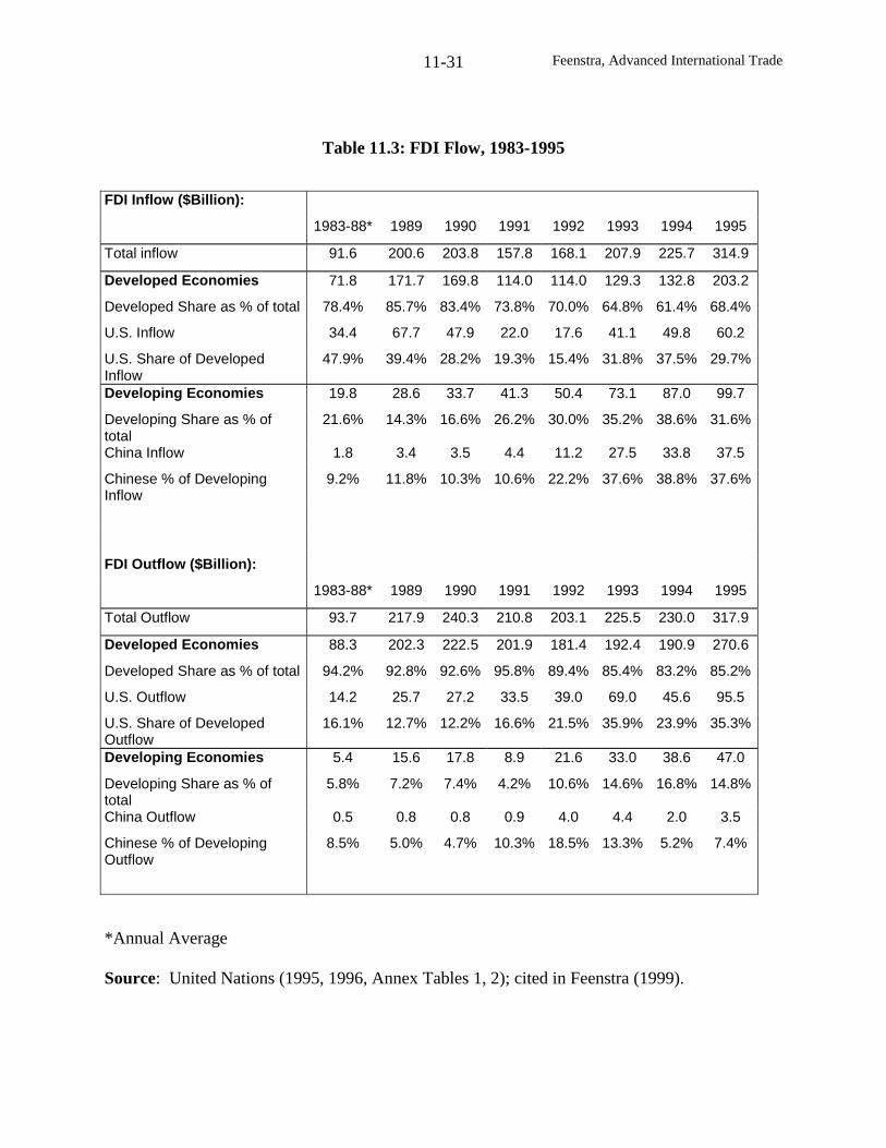
Feenstra, Advanced International Trade11-31
Table 11.3: FDI Flow, 1983-1995
FDI Inflow ($Billion):
1983-88* 1989 1990 1991 1992 1993 1994 1995
Total inflow 91.6 200.6 203.8 157.8 168.1 207.9 225.7 314.9
Developed Economies 71.8 171.7 169.8 114.0 114.0 129.3 132.8 203.2
Developed Share as % of total 78.4% 85.7% 83.4% 73.8% 70.0% 64.8% 61.4% 68.4%
U.S. Inflow 34.4 67.7 47.9 22.0 17.6 41.1 49.8 60.2
U.S. Share of DevelopedInflow
47.9% 39.4% 28.2% 19.3% 15.4% 31.8% 37.5% 29.7%
Developing Economies 19.8 28.6 33.7 41.3 50.4 73.1 87.0 99.7
Developing Share as % oftotal
21.6% 14.3% 16.6% 26.2% 30.0% 35.2% 38.6% 31.6%
China Inflow 1.8 3.4 3.5 4.4 11.2 27.5 33.8 37.5
Chinese % of DevelopingInflow
9.2% 11.8% 10.3% 10.6% 22.2% 37.6% 38.8% 37.6%
FDI Outflow ($Billion):
1983-88* 1989 1990 1991 1992 1993 1994 1995
Total Outflow 93.7 217.9 240.3 210.8 203.1 225.5 230.0 317.9
Developed Economies 88.3 202.3 222.5 201.9 181.4 192.4 190.9 270.6
Developed Share as % of total 94.2% 92.8% 92.6% 95.8% 89.4% 85.4% 83.2% 85.2%
U.S. Outflow 14.2 25.7 27.2 33.5 39.0 69.0 45.6 95.5
U.S. Share of DevelopedOutflow
16.1% 12.7% 12.2% 16.6% 21.5% 35.9% 23.9% 35.3%
Developing Economies 5.4 15.6 17.8 8.9 21.6 33.0 38.6 47.0
Developing Share as % oftotal
5.8% 7.2% 7.4% 4.2% 10.6% 14.6% 16.8% 14.8%
China Outflow 0.5 0.8 0.8 0.9 4.0 4.4 2.0 3.5
Chinese % of DevelopingOutflow
8.5% 5.0% 4.7% 10.3% 18.5% 13.3% 5.2% 7.4%
*Annual Average
Source: United Nations (1995, 1996, Annex Tables 1, 2); cited in Feenstra (1999).
Feenstra, Advanced International Trade11-32
majority of FDI is in developed countries. There was a surge of investment into the developed
countries during the second half of the 1980s, during which time the stock of investment in
developed countries nearly tripled from $538 billion to $1,373 billion. At the same time, there
was a considerable increase in foreign investment into the U.S., which doubled from 1980 to
1985 and again from 1985 to 1990. Since 1990, the stock of investment located in the
developing countries has grown more rapidly, which is in large part due to increased FDI into
China. This country accounts for 18.6% of the inward stock of developing countries in 1995, up
from 4.1% just five years earlier. The vast majority of FDI entering into developed and
developing countries alike comes from the developed countries, as shown in the lower-half of
Table 11.2.
Similar to these stock figures, the majority of FDI flows shown in Table 11.3 are to
developed countries, though China is also a large recipient. For example, in 1995 the United
States received the most FDI, with an inflow of $60.2 billion, but China has the second-largest
inflow of $37.5 billion. The surge in FDI flows during the second half of the 1980s both comes
from and was directed towards the developed countries: this flow reached $172 billion in 1989.
This was followed by a fall in direct investment magnitudes from 1990 to 1991, with a recovery
that was slow at first but has increased recently to reach $203 billion in 1995. The inflow of
investment into China grew most dramatically in 1990-92, and again in 1994-95.
From this very brief examination of the data, it is apparent that the majority of FDI flows
is still between the industrial countries, but that an increasing fraction is being directed towards
the developing countries, especially China. There are two major problems with using such data
to test models of multinationals: first, the types of investments have been changing during the
Feenstra, Advanced International Trade11-33
1990’s; and second, linkages between firms can come from contractual arrangements across
countries that need not be reflected in multinational investments.
On the first problem, Hanson, Mataloni and Slaughter (2001) use a more recent and
detailed dataset to evaluate the types of investments made by U.S. multinationals. These data
include detailed information on the various roles played by foreign affiliates: in importing inputs
from their U.S. parents for further processing; in selling locally within the host countries; and in
exporting from the host countries. The first of these roles illustrate vertical investment while the
second is horizontal investment, and the third could be either. These authors find that both types
of investments are important in the data, with a growing share of vertical investments in some
industries and regions. It is quite possible that pooling the data across industries and countries as
in (11.9) will hide the underlying presence of both activities.
On the second problem, there is no way that data on multinationals will reflect the vast
amount of outsourcing between unaffiliated firms. This is especially true of vertical
relationships. Nike manufactures all of its running shoes in Asia, but does not own these plants;
nevertheless, this is a vertical relationship very much in the spirit of Helpman’s (1984c) model.
So we should not expect data on multinationals alone to give the complete picture of horizontal
and vertical relationships between firms. Estimating the determinants of these in a dataset that
allows for both is therefore a challenge for future empirical research. But it is also a challenge
for theoretical work: we would like to explain the division between activities that are kept
internal to the multinational, and activities that external to the firm. This will be discussed in the
remainder of the chapter.
Feenstra, Advanced International Trade11-34
Organization of the Firm
Both the vertical and horizontal multinational models involved a firm deciding whether to
open an additional plant in a foreign country, but neither of these models addressed the question
of whether the foreign plant had to be owned by the multinational or not. What would prevent
the home firm from entering into a joint venture or some other contractual arrangement with a
foreign firm rather than establishing a new plant? In order to explain this, we need to add a
richer structure to the models we have considered so far. We shall discuss two explanations for
the integration of firms: transactions costs under incomplete contracts; and the “matching” of
firms under incomplete information.17
Transactions Costs
A general reason for the existence of firms provided by Ronald Coase (1937) is that there
are costs involved with making transactions on the markets, and when these costs become too
high, the activities are instead internalized within the firm. This idea was greatly elaborated by
Oliver Williamson (1975, 1985), and is associated with the twin concepts of “asset specificity”
and the “holdup problem.” To explain these, suppose that firm A needs some new input. It
could ask firm B to produce it, but that would be expensive for it to design and test. If firm B
managed to successfully produce it, and then sell it to A, then what guarantee does firm B have
that it will be paid enough to cover its costs of design, let alone its costs of production? If firm
17 There are also other reasons for firm to integrate. Markusen (2001; 2002, chaps. 13-15) develops severalprincipal-agent models of the firms under imperfect information, in which the parent company must give up rents tothe foreign partner to obtain its cooperation. If these rents become too high, the firm will instead integrate acrossborders. In addition, firms may integrate horizontally or vertically to increase their market power and profits, asdiscussed in the industrial organization literature: see Perry and Porter, 1985, Farrell and Shapiro, 1990, Fauli-Oller,2000, and Henrik and Persson, 2001, for the horizontal case; Dixit, 1983, Mathewson and Winter, 1983, Perry andGroff, 1985, Ordover, Salant and Saloner, 1990, 1992, Hart and Tirole, 1990, Abiru et al, 1998, and Chen, 2001, forthe vertical case; as well as the survey by Perry, 1989, and the work of Feenstra, Huang and Hamilton, 2003, thatcombines horizontal and vertical integration within “business groups” and discusses the implications for trade.
Feenstra, Advanced International Trade11-35
A and B could contract in the beginning to specify what the input would cost to develop and
produce, then that would resolve the problem, but it may be difficult to foresee in the beginning
what these costs would be.
In the absence of complete contracts, firm B will be left with an input which may or may
not be useful to buyers other than firm A: this is called “asset specificity.” We can presume that
the better suited is the input to firm A’s needs, then the less valuable it is to alternative buyers.
But in that case, firm B has very little bargaining power in refusing to sell the input to firm A:
this is the “holdup problem.” Because of the holdup problem, firm B might decide to produce an
input that is not very well suited to firm A, but instead can be sold to other purchasers. So the
incomplete contracts lead to an inefficient outcome. If this inefficiency is too great, then firm A
might decide to just design the input itself; i.e. it will vertically integrate into the production of
that good, and thereby become a bigger firm.
From this line of reasoning, we can see that the decision of a firm to integrate depends on
the cost of making market transactions under incomplete contracts, and in particular, asset
specificity and the holdup problem. These insights of Coase and Williamson have only recently
been formalized into models of the firm, and key references are Grossman and Hart (1986), Hart
and Moore (1990, 1999) and Aghion and Tirole (1997). It is even more recent that these ideas
have been incorporated into general equilibrium models of trade, and references include
McLaren (2000), Grossman and Helpman (2002a,b), Marin and Verdier (2001), Antràs (2002)
and Puga and Trefler (2002). These papers are new enough that we do not attempt to summarize
their contributions in this evolving area, but highly recommend them for further reading.
Feenstra, Advanced International Trade11-36
Matching of Firms
Our second explanation for the integration of firms is to share the information that each
has about their own national markets. For example, joint ventures between firms in different
countries can bring with them knowledge of the supplier and distribution networks in each
country, and any other intangible assets owned by either firm. Rauch and Trindade (2000)
model this informational issue as a problem of “matching” firms across countries, where there is
some inherent uncertainty in the ability to find a good partner.18 The starting point for their
analysis is similar to the one-sector model discussed at the beginning of the chapter, where
capital combines with labor to produce a homogeneous good. We now suppose, however, that
two producers must form a joint venture in order to successfully obtain output. These producers
may both be in the same country (as in the autarky equilibrium) or may come from different
countries (in the trade equilibrium with joint ventures). Let us initially focus on the autarky
equilibrium.
The amount of output obtained by two producers depends on their complementarity with
each other. For convenience, we will array the producers in each country around a circle of
circumference unity, as illustrated in Figure 11.5. Let zij denote the shortest arc-distance
between producers of type i and j, which measures their complementarity. Notice that the
maximum value of zij is 1/2. Then we assume that the output obtained by a joint venture of these
producers is yij = f(Lij, zij), where Lij is the labor used. We do not include capital in this
production function since the amount available from each producer is equal and fixed. We
18 The work of Rauch and Trindade (2000) builds upon that in Casella and Rauch (2002) and Rauch and Casella(2003).
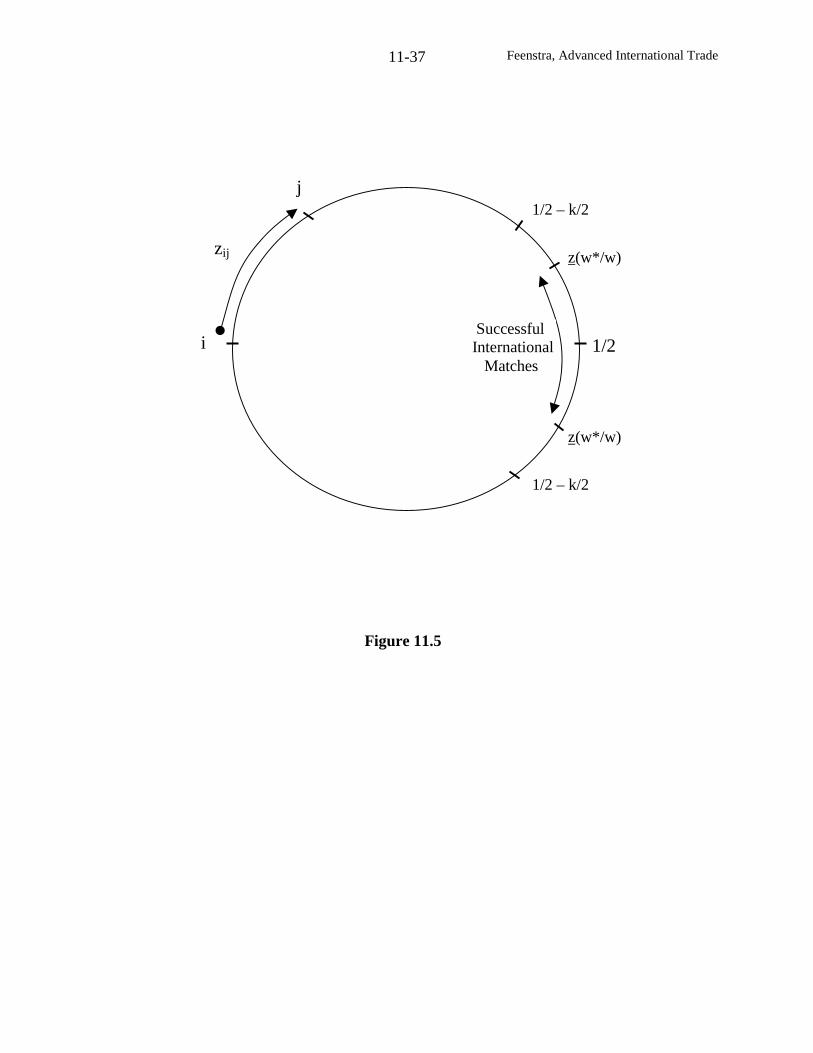
Feenstra, Advanced International Trade11-37
i
j
zij
1/2
1/2 – k/2
1/2 – k/2
z(w*/w)
z(w*/w)
SuccessfulInternational
Matches
Figure 11.5
Feenstra, Advanced International Trade11-38
assume that f(Lij, zij) is increasing and homogeneous of degree one in (Lij, zij), so that producers
farther away from each other obtain higher output.
If labor is available at the wage w, the profits obtained from this joint venture are:
g(w, zij) ≡ ijijijL
maxwL)z,L(f
ij− , (11.10)
where we have normalized the price of the output at unity. Under our assumption that f(Lij, zij)
is homogeneous of degree one in its arguments, then g(w, zij) will be homogeneous of degree
one in zij: increasing the distance zij between producers will lead to an equi-proportionate
increase in labor hired, and in output and profits. It follows that we can write total profits earned
as g(w, zij) = zij π(w), where π(w) ≡ g(w,1). By the envelope theorem, the amount of labor hired
by the joint venture is Lij = – zij π’(w) > 0. Increasing the wage must reduce the labor hired, so
that dLij/dw = – zij π”(w) < 0, which means that π”(w) > 0 so π is convex. For convenience in
our discussion, we follow Rauch and Trindade in assuming that π(w) has the iso-elastic form
π(w) = bw-γ
, with b,γ > 0. This form will apply if the function f(Lij, zij) is Cobb-Douglas.19
To solve for the autarky equilibrium, we need to match up producers in a single country. We
assume that producers are uniformly distributed around the circle in Figure 11.5, and that at each
point on the circle there is a unit-mass of producers: so the total distribution of them can be
thought of as a “unit cylinder.” The best matches are obtained when each producer has a joint
venture with the one located on the opposite side of the circle, so that zij = 1/2. The profits
19 See problem 11.4.
Feenstra, Advanced International Trade11-39
earned from each of these matches are zij π(w) = π(w)/2. We assume that these are equally
divided by the two participants, so each producer earns π(w)/4 in the autarky equilibrium.
The equilibrium wage is determined by equating labor demand and supply. One-half of the
producers are matching with the other half (on the opposite side of the circle), so the total
number of matches is 1/2. It follows that home autarky labor demand is:
– zij π’(wa)/2 = – π’(wa
)/4 = L , (11.11)
where the first equality is obtained because producers are matching with those on the opposite
side of the circle (zij = 1/2), and the second equality sets labor demand equal to the endowment L
to determine the autarky wage wa.
Let us now introduce a foreign country, with the same technology but having a higher
labor endowment L* > L. Under autarky, the foreign wage satisfies – π’( ∗aw )/4 = L*, and
would therefore be lower than at home: ∗aw < wa
since L* > L, using the convexity of π. In the
trade equilibrium we allow joint ventures to form between producers across countries. We
assume that in such a joint venture, the producers can employ labor in either country: given that
foreign wages are lower, they will choose to locate there. This will tend to shift labor demand
away from the labor-scarce home towards the labor-abundant foreign country, and therefore
diminish the difference in their wages. How far will this process of wage equalization proceed?
In the one-sector model used at the beginning of the chapter, full equalization of home and
foreign wages would be achieved through capital mobility. That is, equalization of the rental
rates across countries combined with identical technologies implies that wages are equalized,
Feenstra, Advanced International Trade11-40
too.20 The goal of the matching model is to see how this result is modified when there are some
frictions due to the information problems in finding a good partner.
To this end, suppose that producers can enter into a joint venture across countries. If
these joint ventures prove to be unprofitable, then their “status quo” position is to enter into a
joint venture domestically. Presuming that they still match with a domestic partner at the
opposite side of the circle, then this would result in status quo payoffs of π(w)/4 and π(w*)/4 for
a producer in each country. Notice that these are evaluated at the equilibrium wages with
international joint ventures, which will differ from the autarky wages. The international joint
venture will yield profits of zij π(w*), where zij is the distance between the home and foreign
producers and they employ labor in the foreign country. The two producers will divide the
payoff zij π(w*) between themselves according to some rule, the details of which need not
concern us.21
Given that the total payoff to a home and foreign producer who match domestically is
[π(w)/4 + π(w*)/4], it is apparent that the international joint venture is equally profitable if it
occurs between a home and foreign producer who are distance z apart, with,
z π(w*) = [π(w)/4 + π(w*)/4] ⇔ z(w*/w) = (1/4)[1 + π(w)/π(w*)] . (11.12)
Under our assumption that π(w) takes on the iso-elastic form bw-γ
, with b,γ > 0, we can write
π(w)/π(w*) = (w*/w)γ
as an increasing function of the relative foreign wage, and likewise for
z(w*/w). We will confirm below that foreign wages are less than those at home in the trade
20 See problem 11.5.21 Rauch and Trindade (2000) assume that the payoff zijπ(w*) is divided according to the Nash bargainingsolution.
Feenstra, Advanced International Trade11-41
equilibrium with joint ventures, so that z < 1/2. Recalling that the maximum distance between
any two producers is 1/2, then those international matches in the range zij ∈ (z, 1/2] will be
strictly preferred to domestic matches.
Following Rauch and Trindade, let us add some structure to the international matches.
We will assume that when a home producer i searches for a potential foreign partner j, the
distance between them is randomly drawn from a uniform distribution defined over the interval
[1/2 – k/2, 1/2]. Notice that when k = 1, this interval is [0,1/2], which means that partners are
randomly distributed over the entire circle (recall again that the maximum distance in 1/2). On
the other hand, when k = 0 this interval becomes the point 1/2, which is the best match possible.
So the parameter k∈ [0,1] indexes the extent of uncertainty in international joint ventures.
This structure of international matches is illustrated in Figure 11.5. For a domestic agent
located at the point labeled i, the best match would be at the point labeled 1/2 on the opposite
side of the circle. The range of possible matches are in the interval [1/2 – k/2, 1/2] on either side
of the point 1/2. On the other hand, the successful international matches must satisfy (11.12),
which must be at least the distance z(w*/w) away from the point i.22
We can now compute that probability P that an international match is successful. This is
simply the length of the interval as [z(w*/w), 1/2] as compared to [1/2 – k/2, 1/2], or,
k
)w/*w(z21
)2/k2/1(2/1
)w/*w(z2/1P
−=−−
−= . (11.13)
22 It can be confirmed that z(w*/w) must lie within the interval [1/2 – k/2, 1/2] in equilibrium. If this were not thecase (i.e. if z(w*/w) < 1/2 – k/2) then all home producers would enter into joint ventures with foreign producers,and the demand for home labor would be zero.
Feenstra, Advanced International Trade11-42
Thus, the probability of a successful international match is higher when the ratio of wages w*/w
is lower (meaning that z is lower), or when the uncertainty k associated with international joint
ventures is reduced.
To determine wages we use labor market equilibrium in both countries. Home labor is
demanded only by those domestic producers whose international matches were not successful, or
a fraction (1–P) of home producers. The home demand for labor is therefore:
–(1 – P) π’(w)/4 = L , (11.14)
which can be compared to (11.11). Home labor demand has fallen from autarky due to
producers employing labor abroad, so this results in a fall in the domestic wage, w < wa.
Foreign labor demand has two components. The first is the demand from foreign
producers whose international matches are not successful, and by analogy with (11.14), this is
–(1 – P)π’(w*)/4. However, there is also labor demand from all the successful international
matches. This is computed by taking the expected value of labor demand – zij π’(w*) over the
successful matches in the range zij ∈ (z(w*/w), 1/2] . Therefore, the equilibrium condition in the
foreign labor market is,
– (1 – P)π’(w*)/4 – ∫ π
2/1
)w/*w(z ijij dz*)w('zk
2= L* . (11.15)
Notice that in the integral on the left of (11.15) we have multiplied by (2/k), which is the density
of the uniform distribution of international matches zij over its interval [1/2 – k/2, 1/2], and
converts that integral into an expected value.
Feenstra, Advanced International Trade11-43
Then dividing (11.15) by (11.14), we obtain a single equation to determine the relative
home wage:
(w/w*)γ+1
−
+ ∫2/1
)w/*w(z ijijdzz)P1(k
81 = L*/L , (11.16)
where we have simplified this expression using the iso-elastic form for π(w), so that π’(w*)/π’(w)
= (w/w*)γ+1
. Despite the complexity of (11.16), it is readily shown that the left-hand side is a
strictly increasing function of (w/w*), which starts at unity when (w/w*) =1 and approaches
infinity as (w/w*) →∞.23 It follows that there is a unique solution for (w/w*) from (11.16).
This establishes the first part of the following theorem:
Theorem (Rauch and Trindade, 2000)
(a) The trade equilibrium with international joint ventures exists and is unique;
(b) As k→0 so there is no uncertainly about international partners, then (w/w*)→1;
(c) dw/dk > 0 and dw*/dk < 0;
(d) dln(w/w*)/dln(L*/L) < 1/(1+γ), is increasing in k, and0k
lim
→dln(w/w*)/dln(L*/L) = 0.
Part (b) of this theorem is obtained by inspection of the equilibrium condition (11.16).
As k→0, the term multiplying the integral goes to infinity (meaning that w/w* goes to zero),
unless the lower limit of integration approaches 1/2 so the integral goes to zero. The former case
is easily ruled out as an equilibrium, so as k→0 we must have z → 1/2 in the lower limit of
23 Notice that z(w*/w) is decreasing in (w/w*), which reduces the lower limit of integration so the value of theintegral on the left of (11.16) is increasing in (w/w*). Likewise, P in (11.13) is increasing in (w/w*), and then so is1/(1–P) that appears on the left of (11.16).
Feenstra, Advanced International Trade11-44
integration, which implies that the wages approach equality. Recall that this would be the
outcome in the one-sector model used earlier in the chapter under perfect capital mobility.
Therefore, the matching model approaches the outcome with perfect capital mobility as the
uncertainty about international partners is eliminated. Part (c) of the theorem confirms that as
international uncertainty increases, the equilibrium gets monotonically farther away from wage
equalization: raising k increases domestic wages and lowers foreign wages, as fewer joint
ventures are pursued.
In part (d), Rauch and Trindade investigate the sensitivity of relative wages to changes in
the labor endowments. Notice that from (11.16), if we held z constant (so that P is also
constant), then we readily obtain dln(w/w*)/dln(L*/L) = 1/(1+γ) > 0. Relative wages are
increasing in the relative labor endowment of the other country for fixed z, just as they are in
autarky, because more labor abroad lowers foreign wages. In contrast, when wages are
equalized across countries then dln(w/w*)/dln(L*/L) = 0, as occurs in the one-sector model
under perfect capital mobility used earlier in the chapter. We can interpret this as saying that
perfect capital mobility leads to complete integration of the labor markets. Then part (d) states
that the matching model leads to greater integration of the labor markets than in autarky, and
monotonically approaches the case of perfect capital mobility as uncertainty k approaches zero.
There are many potential empirical and theoretical applications of this matching model.
It is well known that wages do respond to some degree to changes in local labor supplies (see
Bernard and Jensen, 2000), so that labor markets are not fully integrated across regions or
countries. One explanation, according to this model, is the informational frictions involved in
the movement of producers. This outcome is certainly not restricted to the one-sector, two-factor
setting, and would apply equally well to the two-sector HO model. The finding of “factor price
Feenstra, Advanced International Trade11-45
insensitivity” discussed in the HO model (see chapter 1) relies on countries being able to freely
export the goods which use intensively the factors that are growing in abundance.
If there are informational frictions in the ability to match buyers and sellers in international trade,
then factor price insensitivity would no longer hold: a growing labor force, for example, would
necessitate increased exports of the labor-intensive goods, but if buyers are hard to find then we
would expect a terms of trade decline for those goods and therefore falling wages.24
The idea that selling goods on international market requires a “match” between buyers
and sellers is explored empirically by Rauch and Trindade (2002). Earlier work by Gould (1994)
for the U.S. and Head and Ries (1998) for Canada had confirmed the importance of immigrant
networks in promoting trade with their home countries. Rauch and Trindade (2002) expand this
to consider global bilateral trade, and show the importance of Chinese ethnic networks in
enhancing trade. These networks are measured by the level or fraction of the population in a
country that is of Chinese ethnic background, which is entered along with other typical
regressors in a gravity equation.
Following earlier work by Rauch (1999), the trade flows in the gravity equation are
distinguished depending on whether the products are homogeneous, with published prices;
differentiated, with prices that are not available; or an in-between category of “reference priced”
products. It is found that the variable measuring Chinese networks enters most significantly in
the bilateral trade equations for differentiated goods. This supports the idea that the
informational difficulty is assessing these goods is more severe than from homogeneous goods,
and that having traders of the same ethnic background can overcome this difficulty to some
extent.
24 The same logic holds in any large-country model with labor migration. See problem 11.6.
Feenstra, Advanced International Trade11-46
Other empirical results that indicate the informational difficulties in international trade
come from studies of the large traders in Hong Kong, such as Li and Fung (Slater and Amaha,
1999). Their activities include matching firms or consumers who are the buyers of goods, with
the most appropriate producers of the goods, located in China or elsewhere in Asia. The value
of these informational activities to the buyers and sellers involved will depend on the type of
good (homogeneous versus differentiated), uncertainty in prices and quality, market “thickness”,
and income levels of the buyers. Feenstra and Hanson (2001) find that these regressors are
significant explanations of the markups charged on goods re-exported through Hong Kong. This
further indicates the importance of information in allowing for successful “matches” in
international trade.
Conclusions
In this chapter we have reviewed a large literature on the role of foreign direct investment
(FDI) and multinationals on trade. The early contributions of Mundell (1957) and MacDougall
(1960) dealt with capital flows between economies, though FDI can instead involve a change in
ownership and location of firms, without any capital flows. The later contributions of Helpman
(1984c) and Markusen (1984) focused on the decision to establish vertical or horizontal foreign
subsidiaries. The fact that the parent company had invested in headquarters services gave it an
asset that could be transferred to the subsidiary. It was assumed by Helpman and Markusen that
this asset was kept internal to the firm, but of course, these need not be the case: a great deal of
international trade occurs between unaffiliated firms. This creates both an empirical and
theoretical challenge of explaining cross-firm versus within-firm transactions.
At the theoretical level, transactions are kept internal to a firm when the cost of pursuing
them between firms is too great. This is the starting point for the transactions cost explanation
Feenstra, Advanced International Trade11-47
for the organization of the firm. This idea has been elaborated in the recent industrial
organization models of Grossman and Hart (1986), Hart and Moore (1990, 1999) and Aghion
and Tirole (1997), and has just begun to be incorporated into international trade models. This is
a new and exciting topic, which may well replace increasing returns and imperfect competition
(in the 1980s), endogenous growth (in the first half of the 1990s) and political economy (in the
second half of the 1990s) as the next major research area in trade.
One objective of this research is to identify types of trading relationships that lie in-
between the two extremes of market transactions and vertical integration, such as when firms
engage in a joint venture or other ongoing relationship. We can refer to such trade as a “link”
between the two firms, and the set of links between buyers and sellers is referred to as a
“network.”25 As an extension of our study of multinationals, we are naturally led to a discussion
of networks in international trade. These are relationships that represent more than market
transactions, but less than full integration within a firm. There are many types of economic and
social networks that can be considered (Rauch, 2001; Rauch and Casella, 2001), and we have
discussed just one, arising from the “matching” of agents across international borders. Since
firms will want to be linked with good partners abroad, we can expect that agents will find it
profitable to undertake this matching activity. A model along these lines is developed by Rauch
and Watson (2002), where individuals with expertise choose to become “international trade
intermediaries.” This also creates a role for governments to support such intermediation
activities, through trade fairs, associations, etc. Evidently, these ideas are bringing the trader
back into international trade, where he or she should have been all along!
25 This terminology follows Kranton and Minehart (2001).
Feenstra, Advanced International Trade11-48
Problems
Our analysis of capital flows in the HO model compared the equilibrium before and after
the tariff, with a complete flow of capital, it is of interest to ask what happens to the welfare of
the country imposing the tariff during the transition. That is, as the capital inflow moves the
countries from point Vito iV in Figure 11.2, how does the welfare of the capital-importing
country change? This question is addressed by Brecher and Diaz Alejandro (1977). To answer
this, it is useful to work in reverse, and ask what happens if capital leaves the country starting at
the point iV , with the tariff on the capital-intensive good applied by country 1.
The outflow of capital from the point iV will reduce production of the capital-intensive
good in country 1, and increase production of the labor-intensive good. Normally, this would
lead to the capital-intensive good being imported. However, due to the tariff in that industry,
there will be some range of capital outflow that does not lead to any imports; instead, country 1
remains in autarky but with a change in relative prices. You can illustrate this in Figure 11.2 by
labeling a point Ei, lying on the line between V
iand iV , such that for the range of endowments
between iV and Ei, both countries remain in autarky due to the tariff applied by country 1. See
Figure 11.8. Now answer problems 11.1 – 11.3:
11.1 As capital enters country 1, going from Vito E
i, treat international prices as fixed. The
welfare of a representative consumer in that country can be written as V(p,I), where p = p* + t is
the domestic relative price of imports and t is the tariff. As in earlier chapters, we assume that
the exportable is additively separable in utility, so that consumption of the import good is
)p(dp/V −=∂∂ and 1I/V =∂∂ . Total national income equals GDP plus tariff revenue minus
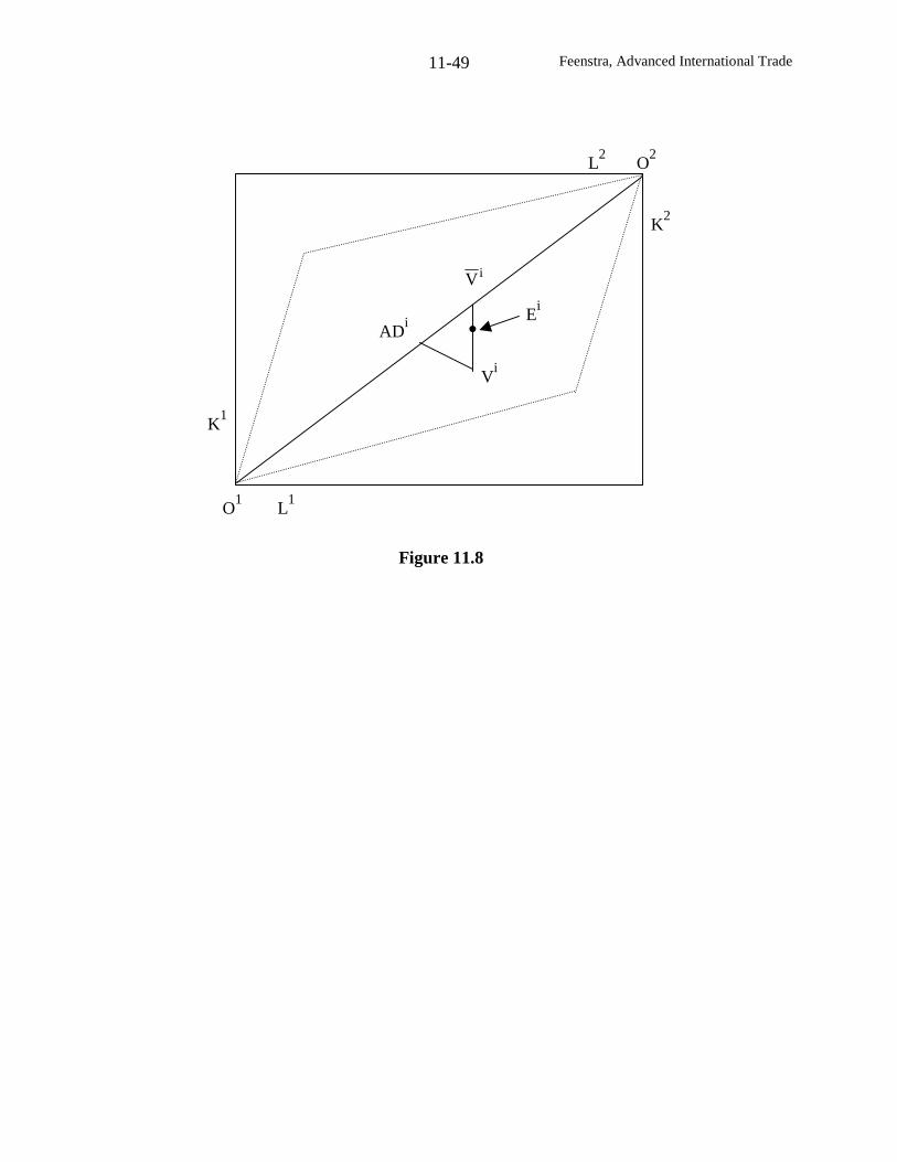
Feenstra, Advanced International Trade11-49
Figure 11.8
ADi
Vi
O1
L1
K1
K2
L2
O2
iV
Ei
Feenstra, Advanced International Trade11-50
payments to foreign capital, so that I = w(p)L + r(p)(K+K*) + tm(p) – r(p)K*, where K* is the
foreign capital, m(p) = d(p) – y(p,L,K+K*) are imports, and y(p,L,K+K*) is production of the
import good, which depends on the labor and capital endowments with the usual Rybczynski
effects. Notice that national income simplifies to I = w(p)L + r(p)K + t[d(p) – y(p,L,K+K*)].
Then differentiate consumer utility with respect to the capital inflow K*, and sign and
interpret this result, assuming that the import good is capital-intensive.
11.2 The results in problem 11.1 apply for inflows of foreign capital between points Viand the
point Ei. At E
i, country 1 is now in autarky. Suppose that capital continues to flow in:
(a) What is the effect of the capital inflow on equilibrium prices for goods, and on the rental?
(b) Thus, what is the effect of the capital inflow on consumer welfare in country 1? (Hint:
illustrate the effect on the rental as in Figure 11.1).
11.3 Summarize your results from problems 11.1 and 11.2 by graphing the relationship between
the capital inflow and welfare of the representative consumer in country 1. How does welfare at
iV compare to the free trade welfare at Vi?
11.4 Suppose that f(Lij, zij) take on the Cobb-Douglas form f(Lij, zij) = )1(ijijzL α−α , 0 < α < 1.
Then solve equation (11.10), and show that π(w) ≡ g(w, 1) can be written in the iso-elastic form
π(w) = bw-γ
, with b,γ > 0.
11.5. In the one-sector model with perfect capital mobility, assume that the technologies are
identical across countries and homogeneous of degree one.
Feenstra, Advanced International Trade11-51
(a) If the rental rates are equalized across countries, what does this imply about the labor-capital
ratios used in production?
(b) Therefore, how do wages compare across countries?
11.6. Rather than capital flows, let us instead consider inflows of labor to a country through
immigration. We will contrast the results of two models:
(a) If there is only one sector in the economy, with fixed capital and fixed output price, then
illustrate the effect of immigration on the home wages, and on welfare.
(b) Suppose instead that we are in a Ricardian model, as discussed in chapter 1. Let labor flow
from the foreign to the home country, and illustrate the impact on the welfare of workers at home
(not including the new migrants). This Ricardian case is discussed in greater detail by Davis and
Weinstein (2002).
Feenstra, Advanced International Trade
Appendix A: Price, Productivity and Terms of Trade Indexes
At various points throughout this book we have relied on index numbers to measure
prices or total factor productivity. There is a good deal of theory, dating back more than a
hundred years, that we can rely on to guide us in the choice of index number formula. Like
econometrics, an understanding of index numbers can be very helpful in empirical research.
Unlike econometrics, these methods are seldom taught. So in this Appendix we present a self-
contained treatment of index numbers, focusing on price indexes.1
We begin with some examples of price indexes. Let p=(p1,…,pN) > 0 denote a vector of
prices, and q=(q1,…,qN) ≥ 0 denote the corresponding vector of quantities. We let pi and qi
denote these vectors in situation i=0,1. We can think of i=0,1 as measuring two time periods, or
later in the Appendix, as measuring two countries. A bilateral index number formula
P(p0,p1,q0,q1) uses just this information on prices and quantities to measure the “average” change
in prices from situation 0 to 1. For example, the Laspeyres price index is:
PL(p0,p1,q0,q1)0i
N1i
0i
1i
N1i
0i
pq
pq
∑∑
=
=≡ . (A1)
Thus, the Laspeyres weights the prices in each period by the quantities in the base period.
Conversely, if we use the current period quantities to weight the prices, we obtain the
Paasche price index:
PP(p0,p1,q0,q1)0i
N1i
1i
1i
N1i
1i
pq
pq
∑∑
=
=≡ . (A2)
1 This Appendix draws extensively from Alterman, Diewert and Feenstra (1999, chapter 2).
Feenstra, Advanced International Trade
A-2
We might expect the Paasche price index to give a lower value than the Laspeyres index when
applied to a consumer choice problem, because by using current period quantities, the Paasche
index incorporates consumer substitution away from goods with the highest price increase. We
will show below that this is indeed the case. A third commonly used formula is Irving Fisher’s
(1922) ideal price index, PF:
PF(p0,p1,q0,q1) ≡ [PL(p0,p1,q0,q1) PP(p0,p1,q0,q1)]1/2 . (A3)
which is the geometric mean of the Laspeyres and Paasche indexes.
Another important formula is the Törnqvist (1936) price index PT, defined as a geometric
mean of the price ratios )p/p( 0i
1i , using as weights the average of the expenditure shares
∑ =≡ N1i
0i
0i
0i
0i
0i qp/qps and ∑ =≡ N
1i1i
1i
1i
1i
1i qp/qps in the two periods:
PT(p0,p1,q0,q1) ∏=
+≡N
1i
2/)ss(0i
1i
1i
0i)p/p( , (A4)
or in logs,
ln PT(p0,p1,q0,q1) ∑=
+=N
1i
0i
1i
1i
0i )p/pln()ss)(2/1( . (A4')
How can we choose between these various formulas? The economic approach to index
numbers is to ask how well each formula reflects the behaviour of consumers or firms. On the
consumer side, we would need to take into account that tastes may be non-homothetic (see
Diewert, 1974, and Pollack, 1989). We will focus here on the problem for firms, where we
consider either an index of the input prices faced by a firm or the output prices. In either case,
we will also want to develop an index of productivity change for the firm, and with an open
economy, an index of the terms of trade.
Feenstra, Advanced International Trade
A-3
Input Price Indexes
Let p = (p1,…pN) denote a positive vector of input prices that producers face in period t,
and let y denote an M dimensional vector of nonnegative outputs that the production sector
might be asked to produce in period t. Then the cost function using period t technology is
defined as:
Ct(p,y) ≡ min q { p'q : (q,y) belongs to St } , (A5)
where St denotes the period t technology set. Thus Ct(p,y) is the minimum cost that the economy
can achieve in period t, given that the vector of outputs y must be produced. Productivity
improvements are reflected in an expansion of the technology set St, and this is why the cost
function Ct(p,y) is also indexed by the period t=0,1.
Generally, the goal of price and productivity indexes will be to measure changes in the
value of costs Ctover time: costs increase as input prices rise, and decrease as productivity
improves. The difficulty is that we do not observe the separate effect of each, but rather, just
observe the total change in costs. We would like to decompose the total change in costs into
components that can be attributed to input prices, productivity, and changes in output.
Toward this end, we can use the function Ctto define the economy’s period t technology
theoretical input price index Pt between any two periods, say period 0 and period 1, as follows:
Pt(p0, p1, y) = Ct(p1,y)/ Ct(p0,y) , (A6)
where pt is the vector of output prices that the economy faces in period t, t = 0,1, and y is a
reference vector of outputs. We refer to this as a “theoretical” index because it cannot be
computed from information on p0, p1, q0, and q1 alone, but also depends on the function Ct. Note
Feenstra, Advanced International Trade
A-4
that this theoretical index has the advantage that it is not influenced by technological change;
rather, it is measured relative to a given period t technology. Our immediate goal is to see
whether, for specific functional forms for the cost function in (A5), there will correspond some
observable price index formula (depending only on prices and quantities p0, p1, q0, and q1) that
will equal (A6), or at least provide upper and lower-bounds to it.
We are interested in two special cases of the theoretical input price index (A6): (a)
P0(p0,p1,y0) which uses the period 0 technology and the output vector y0 that was actually used in
period 0, and (b) P1(p0,p1,y1) which uses the period 1 technology and the output vector y1. Let q0
and q1 be the observed input quantities used in periods 0 and 1, respectively. We assume that
these are optimally chosen to minimize costs in (A5), so that,
C0(p0,y0) = p0'q0 and C1(p1,y1) = p1'q1 . (A7)
Under these cost minimizing assumptions, we can adapt the arguments of Fisher and
Shell (1972, pp. 57-58) and Archibald (1977, p. 66) to show that the two theoretical indexes,
P0(p0, p1, y0) and P1(p0, p1, y1) satisfy the following inequalities:
P0(p0, p1 ,y0) ≡ C0(p1,y0)/ C0(p0,y0) using definition (A6)
= C0(p1,y0)/ p0'q0 using (A7)
≤ p1'q0 / p0'q0 since q0 is feasible for the minimization problem
which defines C0(p1,y0) and so C0(p1,y0) ≤ p1'q0
≡ PL(p0,p1,q0,q1) ,
where PL is the Laspeyres price index. Similarly, we have:
Feenstra, Advanced International Trade
A-5
P1(p0, p1 ,y1) ≡ C1(p1,y1)/ C1(p0,y1) using definition (A6)
= p1'q1/ C1(p0,y1) using (A7)
≥ p1'q1 / p0'q1 since q1 is feasible for the minimization problem
which defines C1(p0,y1) and so C1(p0,y1) ≤ p0'q1
≡ PP(p0,p1,q0,q1) ,
where PP is the Paasche price index. So we find that the Laspeyres index of input prices PL is an
upper bound to the theoretical price index P0(p0, p1 ,y0), and that the Paasche index of input
prices PP is a lower bound to the theoretical price index P1(p0, p1 ,y1). To further explore these
bounds, we separately discuss the cases of constant and changing technology.
Constant Technology
If technology is constant then the Paasche and Laspeyres price indexes provide bounds to
the “true” price index. That is, if technology is constant the cost function can be written as
C(p,y), so the bounds above immediately imply that,
PP(p0,p1,q0,q1) ≤ C(p1,y1)/ C(p0,y1), and C(p1,y0)/ C0(p0,y0) ≤ PL(p0,p1,q0,q1) . (A8)
These expressions can be further simplified by assuming that there is a single output, and that the
technology has constant returns to scale, so that C(p,y) = y c(p), where c(p) is the unit-cost
function. Then the inequalities in (A8) simplify to,
PP(p0,p1,q0,q1) ≤ c(p1)/c(p0) ≤ PL(p0,p1,q0,q1) . (A9)
Thus, we see that the Paasche and Laspeyres price indexes provide lower and upper bounds to
the ratio of unit-costs for the firm, which is the “true” price index. The same would apply to a
Feenstra, Advanced International Trade
A-6
consumer, where we would use the ratio of unit-expenditure functions in the two periods rather
than the ratio of unit-cost. This confirms our assertion above that the Paasche price index is less
than the Laspeyres price index for a consumer choice problem, provided that the quantities used
are optimal for the consumer.
These observations lead us to ask whether it is possible to construct a price index that
exactly equals the ratio of unit-costs, and that is the goal of the economic approach to index
numbers. The strategy is to choose some specific functional form for the cost function, and then
see whether there is a price index formula such that P(p0,p1,q0,q1) = c(p1)/c(p0). For certain
choices of the functional form for costs, it turns out that there is indeed an price index formula
that will satisfy this equality. In this case, Diewert (1976) call the price index exact.
For example, suppose that we choose the quadratic production function 2/1)Aq'q(y = ,
where A=A’ is a symmetric matrix of parameters. It is clear that this production function in
homogeneous of degree one. Diewert (1976, p. 130) shows that this quadratic production
function can approximate any linearly homogeneous function f(q) to the second-order around a
point.2 For this reason, Diewert calls the quadratic function 2/1)Aq'q( a “flexible” functional
form. If A is invertible,3 then it is not difficult to show that the cost function is C(p,y) =
,)Bp'p(y 2/1 where B=A-1, so the unit-cost function becomes c(p) = 2/1)Bp'p( , which is again a
“flexible” functional form.
Then corresponding to the quadratic production and unit-cost functions, we have:
2 That is, the parameters A can be chosen such that 2/1*)Aq*'q( = f(q*), Aq* = fq(q*), and A = fqq(q*), for any
choice of a linearly homogeneous function f(q).3 The solution for the unit-expenditure function when A is not invertible is discussed in Diewert (1976, p. 134).
Feenstra, Advanced International Trade
A-7
Theorem 1 (Diewert, 1976)
If the production and unit-cost functions are quadratic and linearly homogeneous, and the
observed quantities qt > 0 are the cost-minimizing, then:
)p(c
)p(c1
1
= PF(p0,p1,q0,q1) . (A11)
The price index on the right of (A11) is the Fisher ideal formula, defined by (A3), which
is therefore exact for the quadratic unit-cost function. Since the quadratic function is itself
flexible, then Diewert (1976) refers to the Fisher ideal price index as superlative. The
remarkable feature of this theorem is that we achieve equality between the Fisher ideal index and
the ratio of unit-cost function for all values of the parameters A and B. Intuitively, as these
parameters change then so would the optimal choices q, so these choices are “revealing” what
the underlying parameters must be. Using the data on the optimal choices qt, combined with
their prices pt, we are able to measure the ratio of the unit-cost functions in (A11) without
knowing B. This show the power of the economic approach to index numbers.
Changing Technology
With technology changing over time, the situation is more difficult. We are in the
awkward position that the Paasche and Laspeyres indexes provide bounds to a theoretical price
index Pt(p0, p1, y) that itself depends on the period t=0,1. Fortunately, this issue can be resolved,
and it is possible to define a theoretical price index that falls between the observable Paasche and
Laspeyres price indexes. To do this, first we define a hypothetical cost function, C(p,α), that
corresponds to the use of an α-weighted average of the technology sets S0 and S1 for periods 0
Feenstra, Advanced International Trade
A-8
and 1 as the reference technology, and that uses an α-weighted average of the period 0 and
period 1 net output vectors y0 and y1:
C(p,α) ≡ min q { p'q : (q,[1-α]y0 + αy1) belongs to (1- α)S0 + αS1 }. (A11)
We can now use this cost function to define the following family of theoretical price indexes:
P(p0,p1,α) ≡ C(p1,α)/ C(p0,α) . (A12)
We can adapt the proof of Diewert (1983, pp. 1060-1061) and show that there exists an α such
that the theoretical price index defined by (A12) lies between the Paasche and Laspeyres output
indexes, PP and PL :4
Theorem 2 (Diewert, 1983)
There exists α between 0 and 1 such that:
PL ≡ p1'q0 / p0'q0 ≤ P(p0,p1,α) ≤ p1'q1 / p0'q1 ≡ PP or PP ≤ P(p0,p1,α) ≤ PL . (A13)
If the Paasche and Laspeyres indexes are numerically close to each other, then (A13) tells us that
a “true” economic input price index is fairly well determined and we can find a reasonably close
approximation to the “true” index by taking an average of PL and PP, such as Fisher’s ideal price
index PF defined earlier by (A3). This provides a justification for using the Fisher ideal formula
even when the technology is changing.
4 The proofs for all theorems can be found in the sources cited.
Feenstra, Advanced International Trade
A-9
Further results can be obtained by making more specific assumptions on the nature of
technological change. In particular, suppose that the cost function take on the translog
functional form for t = 0,1:5
k
N
1i
M
1ki
tik
M
1k
M
1k
tk2
1
j
N
1i
N
1ji
tij
N
1i
M
1k2
1k
tki
ti
t0
t
ylnplnylnyln
plnplnylnpln)y,p(Cln
∑∑∑∑
∑∑∑ ∑
= == =
= == =
φ+δ+
γ+β+α+α=
ll
l
(A14)
where the parameters satisfy the restrictions tijγ = t
jiγ and,
1N
1i
ti =α∑
=and 0
N
1i
tik
N
1i
tij =φ=γ ∑∑
==. (A15)
These restrictions ensure that Ct(p,y) is linearly homogeneous in the input price vector p (which
is a property that any cost function must satisfy). Note that we are allowing the parameters that
characterize the technology (the α’s, β’s, γ’s, δ’s and φ’s) to be completely different in each
period, reflecting technological change.
Now let us add the restriction that the quadratic price parameters in (A14) are equal
across the two periods, i.e. 0ijγ = 1
ijγ , though we still allow the other parameters to change over
time. Then we can adapt the result in Caves, Christensen and Diewert (1982, pp. 1410) to show
that the geometric mean of the theoretical price indexes in periods 0 and 1, P0(p0,p1,y1) and
P1(p0,p1,y1), is equal to the Törnqvist price index PT defined by (A4):
5 This functional form was introduced and named by Christensen, Jorgenson and Lau (1971). It was adapted to theexpenditure or cost function context by Diewert (1974).
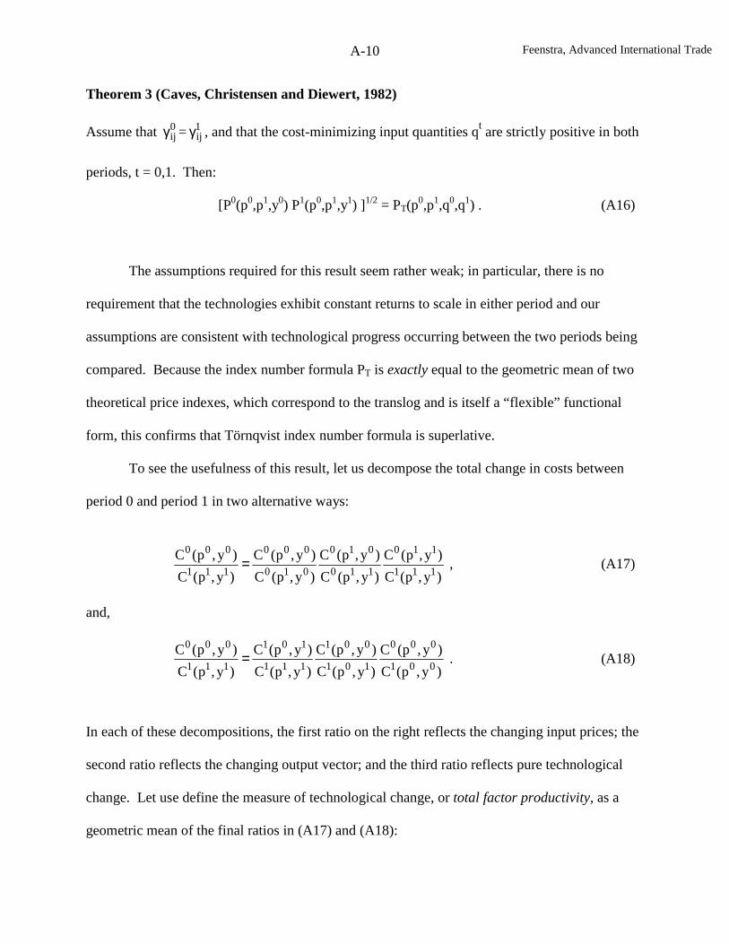
Feenstra, Advanced International Trade
A-10
Theorem 3 (Caves, Christensen and Diewert, 1982)
Assume that 0ijγ = 1
ijγ , and that the cost-minimizing input quantities qt are strictly positive in both
periods, t = 0,1. Then:
[P0(p0,p1,y0) P1(p0,p1,y1) ]1/2 = PT(p0,p1,q0,q1) . (A16)
The assumptions required for this result seem rather weak; in particular, there is no
requirement that the technologies exhibit constant returns to scale in either period and our
assumptions are consistent with technological progress occurring between the two periods being
compared. Because the index number formula PT is exactly equal to the geometric mean of two
theoretical price indexes, which correspond to the translog and is itself a “flexible” functional
form, this confirms that Törnqvist index number formula is superlative.
To see the usefulness of this result, let us decompose the total change in costs between
period 0 and period 1 in two alternative ways:
)y,p(C
)y,p(C
)y,p(C
)y,p(C
)y,p(C
)y,p(C
)y,p(C
)y,p(C111
110
110
010
010
000
111
000
= , (A17)
and,
)y,p(C
)y,p(C
)y,p(C
)y,p(C
)y,p(C
)y,p(C
)y,p(C
)y,p(C001
000
101
001
111
101
111
000
= . (A18)
In each of these decompositions, the first ratio on the right reflects the changing input prices; the
second ratio reflects the changing output vector; and the third ratio reflects pure technological
change. Let use define the measure of technological change, or total factor productivity, as a
geometric mean of the final ratios in (A17) and (A18):
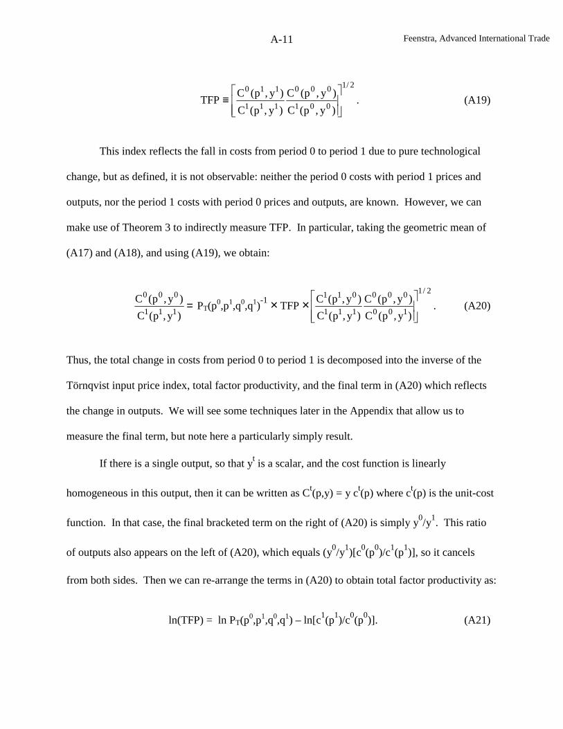
Feenstra, Advanced International Trade
A-11
2/1
001
000
111
110
)y,p(C
)y,p(C
)y,p(C
)y,p(CTFP
≡ . (A19)
This index reflects the fall in costs from period 0 to period 1 due to pure technological
change, but as defined, it is not observable: neither the period 0 costs with period 1 prices and
outputs, nor the period 1 costs with period 0 prices and outputs, are known. However, we can
make use of Theorem 3 to indirectly measure TFP. In particular, taking the geometric mean of
(A17) and (A18), and using (A19), we obtain:
=)y,p(C
)y,p(C111
000
PT(p0,p1,q0,q1)-1 × TFP ×
2/1
100
000
111
011
)y,p(C
)y,p(C
)y,p(C
)y,p(C
. (A20)
Thus, the total change in costs from period 0 to period 1 is decomposed into the inverse of the
Törnqvist input price index, total factor productivity, and the final term in (A20) which reflects
the change in outputs. We will see some techniques later in the Appendix that allow us to
measure the final term, but note here a particularly simply result.
If there is a single output, so that yt is a scalar, and the cost function is linearly
homogeneous in this output, then it can be written as Ct(p,y) = y ct(p) where ct(p) is the unit-cost
function. In that case, the final bracketed term on the right of (A20) is simply y0/y1. This ratio
of outputs also appears on the left of (A20), which equals (y0/y1)[c0(p0)/c1(p1)], so it cancels
from both sides. Then we can re-arrange the terms in (A20) to obtain total factor productivity as:
ln(TFP) = ln PT(p0,p1,q0,q1) – ln[c1(p1)/c0(p0)]. (A21)
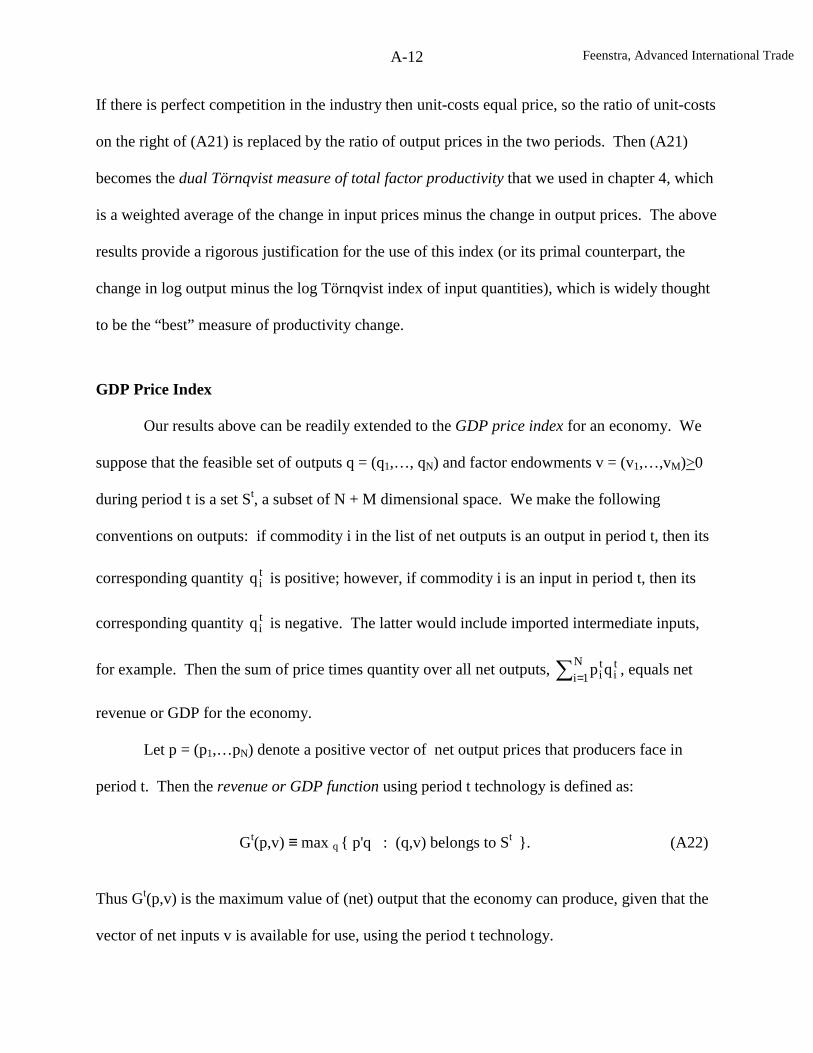
Feenstra, Advanced International Trade
A-12
If there is perfect competition in the industry then unit-costs equal price, so the ratio of unit-costs
on the right of (A21) is replaced by the ratio of output prices in the two periods. Then (A21)
becomes the dual Törnqvist measure of total factor productivity that we used in chapter 4, which
is a weighted average of the change in input prices minus the change in output prices. The above
results provide a rigorous justification for the use of this index (or its primal counterpart, the
change in log output minus the log Törnqvist index of input quantities), which is widely thought
to be the “best” measure of productivity change.
GDP Price Index
Our results above can be readily extended to the GDP price index for an economy. We
suppose that the feasible set of outputs q = (q1,…, qN) and factor endowments v = (v1,…,vM)>0
during period t is a set St, a subset of N + M dimensional space. We make the following
conventions on outputs: if commodity i in the list of net outputs is an output in period t, then its
corresponding quantity tiq is positive; however, if commodity i is an input in period t, then its
corresponding quantity tiq is negative. The latter would include imported intermediate inputs,
for example. Then the sum of price times quantity over all net outputs, ti
N1i
ti qp∑ = , equals net
revenue or GDP for the economy.
Let p = (p1,…pN) denote a positive vector of net output prices that producers face in
period t. Then the revenue or GDP function using period t technology is defined as:
Gt(p,v) ≡ max q { p'q : (q,v) belongs to St }. (A22)
Thus Gt(p,v) is the maximum value of (net) output that the economy can produce, given that the
vector of net inputs v is available for use, using the period t technology.
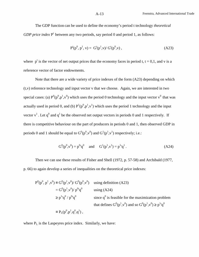
Feenstra, Advanced International Trade
A-13
The GDP function can be used to define the economy’s period t technology theoretical
GDP price index Pt between any two periods, say period 0 and period 1, as follows:
Pt(p0, p1, v) = Gt(p1,v)/ Gt(p0,v) , (A23)
where pt is the vector of net output prices that the economy faces in period t, t = 0,1, and v is a
reference vector of factor endowments.
Note that there are a wide variety of price indexes of the form (A23) depending on which
(t,v) reference technology and input vector v that we choose. Again, we are interested in two
special cases: (a) P0(p0,p1,v0) which uses the period 0 technology and the input vector v0 that was
actually used in period 0, and (b) P1(p0,p1,v1) which uses the period 1 technology and the input
vector v1 . Let q0 and q1 be the observed net output vectors in periods 0 and 1 respectively. If
there is competitive behaviour on the part of producers in periods 0 and 1, then observed GDP in
periods 0 and 1 should be equal to G0(p0,v0) and G1(p1,v1) respectively; i.e.:
G0(p0,v0) = p0'q0 and G1(p1,v1) = p1'q1 . (A24)
Then we can use these results of Fisher and Shell (1972, p. 57-58) and Archibald (1977,
p. 66) to again develop a series of inequalities on the theoretical price indexes:
P0(p0, p1 ,v0) ≡ G0(p1,v0)/ G0(p0,v0) using definition (A23)
= G0(p1,v0)/ p0'q0 using (A24)
≥ p1'q0 / p0'q0 since q0 is feasible for the maximization problem
that defines G0(p1,v0) and so G0(p1,v0) ≥ p1'q0
≡ PL(p0,p1,q0,q1) ,
where PL is the Laspeyres price index. Similarly, we have:
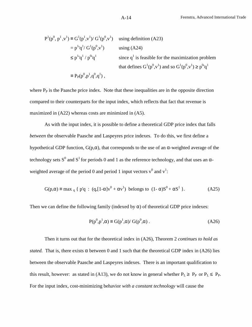
Feenstra, Advanced International Trade
A-14
P1(p0, p1 ,v1) ≡ G1(p1,v1)/ G1(p0,v1) using definition (A23)
= p1'q1/ G1(p0,v1) using (A24)
≤ p1'q1 / p0'q1 since q1 is feasible for the maximization problem
that defines G1(p0,v1) and so G1(p0,v1) ≥ p0'q1
≡ PP(p0,p1,q0,q1) ,
where PP is the Paasche price index. Note that these inequalities are in the opposite direction
compared to their counterparts for the input index, which reflects that fact that revenue is
maximized in (A22) whereas costs are minimized in (A5).
As with the input index, it is possible to define a theoretical GDP price index that falls
between the observable Paasche and Laspeyres price indexes. To do this, we first define a
hypothetical GDP function, G(p,α), that corresponds to the use of an α-weighted average of the
technology sets S0 and S1 for periods 0 and 1 as the reference technology, and that uses an α-
weighted average of the period 0 and period 1 input vectors v0 and v1:
G(p,α) ≡ max q { p'q : (q,[1-α]v0 + αv1) belongs to (1- α)S0 + αS1 }. (A25)
Then we can define the following family (indexed by α) of theoretical GDP price indexes:
P(p0,p1,α) ≡ G(p1,α)/ G(p0,α) . (A26)
Then it turns out that for the theoretical index in (A26), Theorem 2 continues to hold as
stated. That is, there exists α between 0 and 1 such that the theoretical GDP index in (A26) lies
between the observable Paasche and Laspeyres indexes. There is an important qualification to
this result, however: as stated in (A13), we do not know in general whether PL ≥ PP or PL ≤ PP.
For the input index, cost-minimizing behavior with a constant technology will cause the
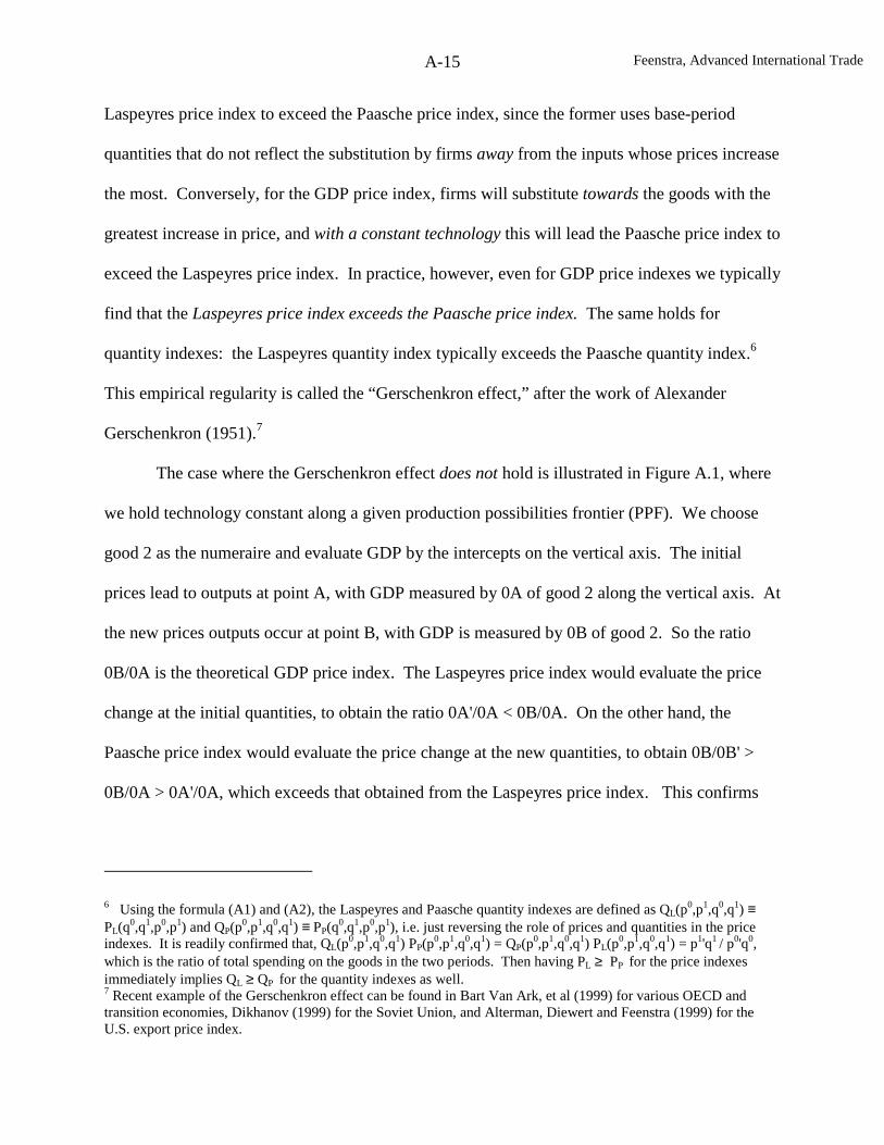
Feenstra, Advanced International Trade
A-15
Laspeyres price index to exceed the Paasche price index, since the former uses base-period
quantities that do not reflect the substitution by firms away from the inputs whose prices increase
the most. Conversely, for the GDP price index, firms will substitute towards the goods with the
greatest increase in price, and with a constant technology this will lead the Paasche price index to
exceed the Laspeyres price index. In practice, however, even for GDP price indexes we typically
find that the Laspeyres price index exceeds the Paasche price index. The same holds for
quantity indexes: the Laspeyres quantity index typically exceeds the Paasche quantity index.6
This empirical regularity is called the “Gerschenkron effect,” after the work of Alexander
Gerschenkron (1951).7
The case where the Gerschenkron effect does not hold is illustrated in Figure A.1, where
we hold technology constant along a given production possibilities frontier (PPF). We choose
good 2 as the numeraire and evaluate GDP by the intercepts on the vertical axis. The initial
prices lead to outputs at point A, with GDP measured by 0A of good 2 along the vertical axis. At
the new prices outputs occur at point B, with GDP is measured by 0B of good 2. So the ratio
0B/0A is the theoretical GDP price index. The Laspeyres price index would evaluate the price
change at the initial quantities, to obtain the ratio 0A'/0A < 0B/0A. On the other hand, the
Paasche price index would evaluate the price change at the new quantities, to obtain 0B/0B' >
0B/0A > 0A'/0A, which exceeds that obtained from the Laspeyres price index. This confirms
6 Using the formula (A1) and (A2), the Laspeyres and Paasche quantity indexes are defined as QL(p0,p1,q0,q1) ≡PL(q0,q1,p0,p1) and QP(p0,p1,q0,q1) ≡ PP(q0,q1,p0,p1), i.e. just reversing the role of prices and quantities in the priceindexes. It is readily confirmed that, QL(p0,p1,q0,q1) PP(p0,p1,q0,q1) = QP(p0,p1,q0,q1) PL(p0,p1,q0,q1) = p1'q1 / p0'q0,which is the ratio of total spending on the goods in the two periods. Then having PL ≥ PP for the price indexesimmediately implies QL ≥ QP for the quantity indexes as well.7 Recent example of the Gerschenkron effect can be found in Bart Van Ark, et al (1999) for various OECD andtransition economies, Dikhanov (1999) for the Soviet Union, and Alterman, Diewert and Feenstra (1999) for theU.S. export price index.
Feenstra, Advanced International Trade
A-16
A
B
B
A'
A
B'
q1
Figure A.1
B
AB
B'
A
C
C'
C
q1
Figure A.2
U
q2
q2
0
0
Feenstra, Advanced International Trade
A-17
that the Paasche price index exceeds the Laspeyres index when technology does not change, due
to output substitution by producers.
In Figure A.2, by contrast, we suppose that the PPF is shifting out due to technological
change. At unchanged prices, GDP would increase from point A to point B (i.e. GDP would
increase from the intercept of AA and BB with the vertical axis). Suppose, however, that the
relative price of good 1 falls due to its increased supply, so that the slope of the line CC shows
the new prices. Production now occurs at point B' rather than point B. We have drawn the case
where the budget lines AA and CC are both tangent to an indifference curve U, indicating that
the change in equilibrium prices are due to changing supply with constant tastes. Thus, the
change in prices will reflect consumer substitution rather than producer substitution.
In the case we have illustrated, the production points A and B' lie on the same ray from
the origin, so that the relative outputs of the two goods are unchanged. This means that the
Laspeyres and Paasche price indexes, using the outputs at points A or B', would be identical. In
fact, evaluating the Laspeyres price index using the initial outputs at point A, we would obtain
GDP of 0A along the vertical axis at the old prices and 0C' at the new prices, so the price index
is 0C'/0A < 1, indicating a substantial fall in the price of good 1. The Paasche price index,
evaluated at the outputs at point B', would give exactly the same result. If point B' occurred
along the PPF slightly to the right, however, then the higher supply of good 1, whose relative
price has fallen, would cause the Paasche price index to be less than the Laspeyres price index.
This would illustrate the Gerschenkron effect.
Finding that the Laspeyres output index exceeds the Paasche is indirect evidence of
changing technology or factor endowments, so that equilibrium prices reflect consumer
substitution rather than producer substitution. The theoretical GDP price index P(p0,p1,α),
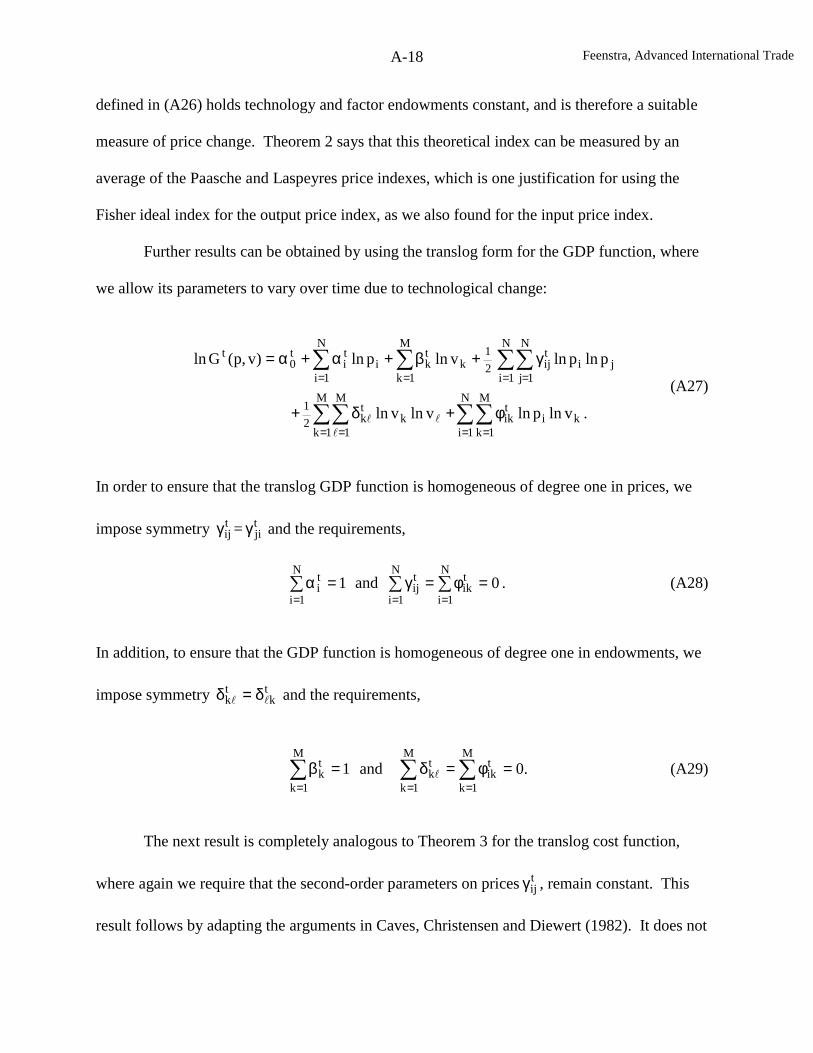
Feenstra, Advanced International Trade
A-18
defined in (A26) holds technology and factor endowments constant, and is therefore a suitable
measure of price change. Theorem 2 says that this theoretical index can be measured by an
average of the Paasche and Laspeyres price indexes, which is one justification for using the
Fisher ideal index for the output price index, as we also found for the input price index.
Further results can be obtained by using the translog form for the GDP function, where
we allow its parameters to vary over time due to technological change:
.vlnplnvlnvln
plnplnvlnpln)v,p(Gln
k
N
1i
M
1ki
tik
M
1k
M
1k
tk2
1
j
N
1i
N
1ji
tij
N
1i
M
1k2
1k
tki
ti
t0
t
∑∑∑∑
∑∑∑ ∑
= == =
= == =
φ+δ+
γ+β+α+α=
ll
l
(A27)
In order to ensure that the translog GDP function is homogeneous of degree one in prices, we
impose symmetry tijγ = t
jiγ and the requirements,
1N
1i
ti =α∑
=and 0
N
1i
tik
N
1i
tij =φ=γ ∑∑
==. (A28)
In addition, to ensure that the GDP function is homogeneous of degree one in endowments, we
impose symmetry tk
tk ll δ=δ and the requirements,
.0and1M
1k
tik
M
1k
tk
M
1k
tk =φ=δ=β ∑∑∑
===l (A29)
The next result is completely analogous to Theorem 3 for the translog cost function,
where again we require that the second-order parameters on prices tijγ , remain constant. This
result follows by adapting the arguments in Caves, Christensen and Diewert (1982). It does not
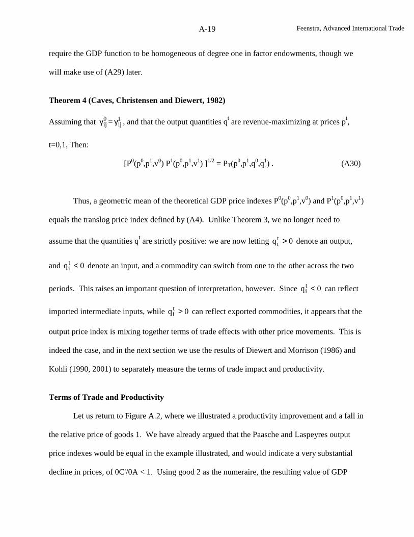
Feenstra, Advanced International Trade
A-19
require the GDP function to be homogeneous of degree one in factor endowments, though we
will make use of (A29) later.
Theorem 4 (Caves, Christensen and Diewert, 1982)
Assuming that 0ijγ = 1
ijγ , and that the output quantities qt are revenue-maximizing at prices pt,
t=0,1, Then:
[P0(p0,p1,v0) P1(p0,p1,v1) ]1/2 = PT(p0,p1,q0,q1) . (A30)
Thus, a geometric mean of the theoretical GDP price indexes P0(p0,p1,v0) and P1(p0,p1,v1)
equals the translog price index defined by (A4). Unlike Theorem 3, we no longer need to
assume that the quantities qt are strictly positive: we are now letting 0qti > denote an output,
and 0qti < denote an input, and a commodity can switch from one to the other across the two
periods. This raises an important question of interpretation, however. Since 0qti < can reflect
imported intermediate inputs, while 0qti > can reflect exported commodities, it appears that the
output price index is mixing together terms of trade effects with other price movements. This is
indeed the case, and in the next section we use the results of Diewert and Morrison (1986) and
Kohli (1990, 2001) to separately measure the terms of trade impact and productivity.
Terms of Trade and Productivity
Let us return to Figure A.2, where we illustrated a productivity improvement and a fall in
the relative price of goods 1. We have already argued that the Paasche and Laspeyres output
price indexes would be equal in the example illustrated, and would indicate a very substantial
decline in prices, of 0C'/0A < 1. Using good 2 as the numeraire, the resulting value of GDP
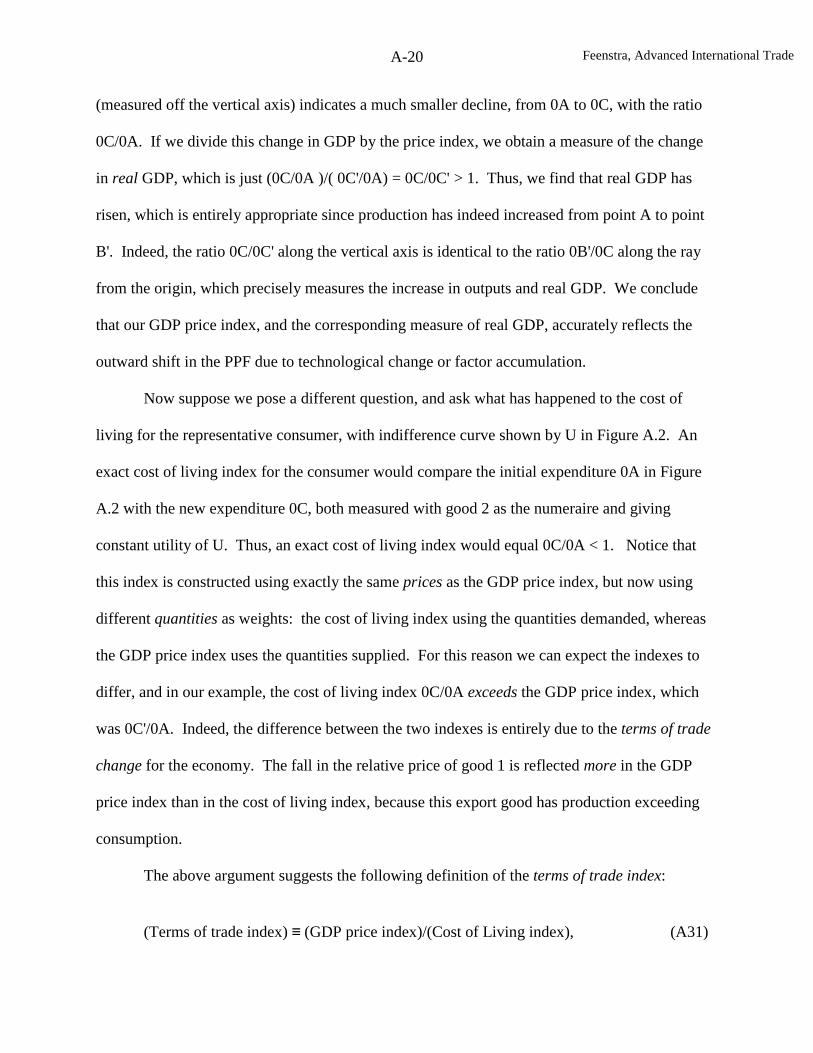
Feenstra, Advanced International Trade
A-20
(measured off the vertical axis) indicates a much smaller decline, from 0A to 0C, with the ratio
0C/0A. If we divide this change in GDP by the price index, we obtain a measure of the change
in real GDP, which is just (0C/0A )/( 0C'/0A) = 0C/0C' > 1. Thus, we find that real GDP has
risen, which is entirely appropriate since production has indeed increased from point A to point
B'. Indeed, the ratio 0C/0C' along the vertical axis is identical to the ratio 0B'/0C along the ray
from the origin, which precisely measures the increase in outputs and real GDP. We conclude
that our GDP price index, and the corresponding measure of real GDP, accurately reflects the
outward shift in the PPF due to technological change or factor accumulation.
Now suppose we pose a different question, and ask what has happened to the cost of
living for the representative consumer, with indifference curve shown by U in Figure A.2. An
exact cost of living index for the consumer would compare the initial expenditure 0A in Figure
A.2 with the new expenditure 0C, both measured with good 2 as the numeraire and giving
constant utility of U. Thus, an exact cost of living index would equal 0C/0A < 1. Notice that
this index is constructed using exactly the same prices as the GDP price index, but now using
different quantities as weights: the cost of living index using the quantities demanded, whereas
the GDP price index uses the quantities supplied. For this reason we can expect the indexes to
differ, and in our example, the cost of living index 0C/0A exceeds the GDP price index, which
was 0C'/0A. Indeed, the difference between the two indexes is entirely due to the terms of trade
change for the economy. The fall in the relative price of good 1 is reflected more in the GDP
price index than in the cost of living index, because this export good has production exceeding
consumption.
The above argument suggests the following definition of the terms of trade index:
(Terms of trade index) ≡ (GDP price index)/(Cost of Living index), (A31)
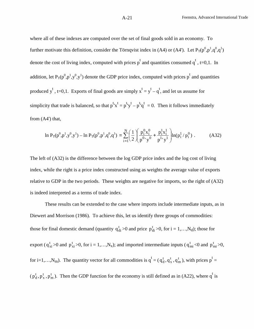
Feenstra, Advanced International Trade
A-21
where all of these indexes are computed over the set of final goods sold in an economy. To
further motivate this definition, consider the Törnqvist index in (A4) or (A4'). Let PT(p0,p1,q0,q1)
denote the cost of living index, computed with prices ptand quantities consumed q
t, t=0,1. In
addition, let PT(p0,p1,y0,y1) denote the GDP price index, computed with prices ptand quantities
produced yt, t=0,1. Exports of final goods are simply x
t= y
t– q
t, and let us assume for
simplicity that trade is balanced, so that pt'x
t= p
t'y
t– p
t'q
t= 0. Then it follows immediately
from (A4') that,
ln PT(p0,p1,y0,y1) – ln PT(p0,p1,q0,q1) ∑=
+
=
N
1i
0i
1i11
1i
1i
00
0i
0i )p/pln(
y'p
xp
y'p
xp
2
1. (A32)
The left of (A32) is the difference between the log GDP price index and the log cost of living
index, while the right is a price index constructed using as weights the average value of exports
relative to GDP in the two periods. These weights are negative for imports, so the right of (A32)
is indeed interpreted as a terms of trade index.
These results can be extended to the case where imports include intermediate inputs, as in
Diewert and Morrison (1986). To achieve this, let us identify three groups of commodities:
those for final domestic demand (quantity tdiq >0 and price t
dip >0, for i = 1,…,Nd); those for
export ( txiq >0 and t
xip >0, for i = 1,…,Nx); and imported intermediate inputs ( tmiq <0 and t
mip >0,
for i=1,…,Nm). The quantity vector for all commodities is qt= ( t
dq , txq , t
mq ), with prices pt=
( tdp , t
xp , tmp ). Then the GDP function for the economy is still defined as in (A22), where q
tis
Feenstra, Advanced International Trade
A-22
the revenue-maximizing choices by firms. We will suppose that GDP takes on the translog form
as in (A27)-(A29).
For this GDP function, let us define the theoretical productivity index:
R(p,v) = G1(p,v)/ G0(p,v) . (A33)
Thus, this theoretical index holds prices and factor endowments fixed, and considers only the
change in productivity between periods 0 and 1. We are interested in two special cases: (a) the
Laspeyres productivity index, RL ≡ R(p0,v
0) = G1(p
0,v
0)/ G0(p
0,v
0), which uses prices and
endowments from period 0; (b) the Paasche productivity index, RP ≡ R(p1,v
1) = G1(p
1,v
1)/
G1(p1,v
1), which uses prices and endowments from period 1. Each of these are unobservable,
but as in our earlier discussion of productivity in (A19)-(A21), we can measure their geometric
mean:
Theorem 5 (Diewert and Morrison, 1986)
Assuming that the GDP function takes on the translog form in (A27)-(A29), and the revenue-
maximizing quantities qtare non-zero, then:
(RL RP)1/2
=
00
11
q'p
q'p/ [PT(p0,p1,q0,q1) QT(w0,w1,v0,v1)]. (A34)
The first term on the right of (A34) is the ratio of GDP in the two periods, or the growth
in nominal GDP. This is deflated by the two other terms on the right: the first is the Törnqvist
Feenstra, Advanced International Trade
A-23
price index of GDP using the formula in (A4); and the second is a Törnqvist quantity index of
factor endowments, defined by:
ln QT(w0,w1,v0,v1) ∑=
+
≡
N
1i
0i
1i11
1i
1i
00
0i
0i )v/vln(
v'w
vw
v'w
vw
2
1. (A35)
Thus, this is a factor-share weighted average of the growth in primary inputs for the economy.
Notice that under our assumption (A29) that the GDP function is linearly homogeneous in v,
then pt'q
t= w
t'v
t, so the shares in the Törnqvist price index and the Törnqvist quantity index are
both measured relative to GDP. Theorem 5 generalizes our earlier derivation of TFP in (A19)-
(A21), to allow now for multiple inputs and outputs.
Let us now take the Törnqvist price index of GDP that appears on the right of (A34), and
decompose it into the portion dealing with domestic goods, exports, and imports:
ln PT(p0,p1,q0,q1) ∑=
+
=
dN
1i
0di
1di11
1di
1di
00
0di
0di )p/pln(
q'p
qp
q'p
qp
2
1(A36)
+ ∑∑==
+
+
+
mx N
1i
0mi
1mi11
1mi
1mi
00
0mi
0mi
N
1i
0xi
1xi11
1xi
1xi
00
0xi
0xi )p/pln(
q'p
qp
q'p
qp
2
1)p/pln(
q'p
qp
q'p
qp
2
1.
We will refer to the first summation on the right of (A36) as the cost of living index, because it
uses the quantities and prices of final goods demanded by the consumer. The exponent of this
first summation is denoted by the Törnqvist price index PT( 0dp , 1
dp , 0dq , 1
dq ), where the shares are
computed relative to total GDP pt'q
t. The second and third terms are the difference between the
export and import price indexes, respectively, where recall that 0qtmi < . Let us denote the
Feenstra, Advanced International Trade
A-24
exponent of these two summations by the Törnqvist index PT( 0xmp , 1
xmp , 0xmq , 1
xmq ), where
again, the shares are computed relative to total GDP pt'q
t.
Then we can re-write the result in (A34) in the following form:
00
11
q'p
q'p= (RLRP)
1/2PT( 0
dp , 1dp , 0
dq , 1dq ) PT )q,q,p,p( 1
xm0xm
1xm
0xm QT(w0,w1,v0,v1). (A37)
Thus, the ratio of nominal GDP is decomposed as a total factor productivity index, a cost of
living price index, a terms of trade index, and a quantity index of endowment growth. Kohli
(2001) argues that if we wish to deflate the growth in GDP to obtain a measure of welfare change
for the representative consumer, then we should use the cost of living index rather than the GDP
price index as a deflator. That is, a measure of welfare change would be,
00
11
q'p
q'p/ PT( 0
dp , 1dp , 0
dq , 1dq ) = (RLRP)
1/2PT )q,q,p,p( 1
xm0xm
1xm
0xm QT(w0,w1,v0,v1). (A38)
This decomposition allows productivity growth, improvements in the terms of trade, and
endowment growth in factors to all contribute positively to welfare. Notice that this measure of
welfare is quite different from how the growth in real GDP is normally calculated, which is to
deflate the ratio of nominal GDP by the GDP price index, obtaining,
00
11
q'p
q'p/ PT(p0,p1,q0,q1) = (RLRP)
1/2QT(w0,w1,v0,v1). (A39)
The log of (A39) is reported as real GDP growth in national income statistics, but it
leaves out changes in the terms of trade as a source of welfare gain. In (A38), by contrast, we
Feenstra, Advanced International Trade
A-25
deflate nominal GDP by the price index computed for domestic goods only, i.e. by the price
index for domestic absorption, C+I+G. By applying this cost of living index to all components
of GDP, C+I+G+X-M, including exports and imports, we obtain a measure of “real welfare” that
is more appropriate to assess changes in the representative consumer. Kohli (1990b, 2001)
shows that deflating nominal GDP by the cost of living index leads to a considerably higher
growth in “real welfare” for some countries (such as Switzerland) that real GDP growth. This is
explained by the terms of trade improvements for such countries in recent years.
Feenstra, Advanced International Trade
Appendix B: Discrete Choice Models
Discrete choice models are commonly taught in econometrics, but the economic
generality of these models is sometimes unclear. This is especially true when we consider
models that incorporate not just demand but also the optimal prices charged by firms under
imperfect competition. In that case, we want to derive demand and prices in a mutually
consistent fashion, as will be discussed in this Appendix.
We begin with an aggregation theorem due to McFadden (1978, 1981). He has shown
that when individual have random utility over discrete alternatives, the decisions that they made
can sometimes be aggregated up to a representative consumer. McFadden focuses on the case
where individual have utility functions that are linear in income, and where the goods over which
a discrete choice is being made are purchased in the quantity 0 or 1. Under certain conditions, it
is possible to generalize this to the case where utility is nonlinear in income, and where the
discrete-choice good is purchased in continuous quantities. This is a principal result of
Anderson, de Palma and Thisse (1992, chaps. 2-5) who show, for example, that the
representative consumer can have a CES utility function, as we also demonstrate below.
At the same time as presenting these aggregation results, we will discuss the empirical
strategy to estimate discrete choice models due to Berry (1994). In this approach, we suppose
that the individual-level data on consumer choices is not available. Rather, we just observe the
market-level data on the quantity purchased of each product, as well as their prices and
characteristics. The goal is to infer the individual taste parameters from this market-level data on
quantities and prices, as well as parameters of marginal cost, so that price-cost margins can be
estimated.
Feenstra, Advanced International TradeB-2
Discrete Choice Model
Suppose there is a population of consumers h, and we normalize its size to unity. Each
consumer must decide which of a discrete number of alternatives j=1,…,N to purchase, and
receives the following utility from consuming one unit of product j:
hjj
hj uV ε+= , (B1)
where uj is the utility obtained from product j by every consumer, while hjε is an additional part
of utility obtained by consumer h. We will treat hjε as a random variable with cumulative
density function F(ε), where each consumer obtains a different draw of ε = (ε1,…,εN). Given
this draw, the consumer chooses the product with highest utility. The probability that a
consumer will choose product j is:
.]N1,...,kallfor,uuProb[
]N1,...,kallfor,uuProb[
]N1,...,kallfor,VVProb[P
jkkj
kkjj
kjj
=−≥ε−ε=
=ε+≥ε+=
=≥=
(B2)
We can think of (B2) as the probability that any consumer choose alternative j, or
equivalently, as the expected fraction of the population that chooses that alternative. The
solution for these choice probabilities depends on the distribution function F(ε), as well as on the
specification of utility uj. A simplified version of utility used by Berry (1994) is,
uj = y + β’zj – αpj + ξj , α > 0. (B3)
Feenstra, Advanced International TradeB-3
Thus, utility is linear in individual income y, decreasing in the price pj, and also depends on the
characteristics zj of the product. 1 The term ξj is another random element in utility, but unlike
hjε , it does not vary across consumers. We could think of ξj as some unmeasured characteristics
of product j, which is random across products but not consumers.
In general, computing the choice probabilities from (B2) is computationally intensive
since it requires integration over various subsets of the domain of F(ε). However, McFadden has
shown that for a class of distribution functions F(ε) known as the generalized extreme value, the
expected demands can be equivalently obtained by simple differentiation:
Theorem 1 (McFadden, 1978, p. 80; 1981, p. 227)
Let H be a nonnegative function defined over NR + that satisfies the following properties:
(i) H is homogeneous of degree one;
(ii) ∞→H as any of its argument approaches infinity;
(iii) The mixed partial derivatives of H with respect to k variables exist and are continuous,
non-negative if k is odd and non-positive if k is even, k=1,…,N.
Define the generalized extreme value distribution function,
)]e...,e,e(Hexp[),...,(F N21 ,N1ε−ε−ε−−≡εε . (B4)
Then the expected value of consumer utility (up to a constant) is given by the aggregate utility
function,
1 This utility function is not homogeneous of degree zero in income y and price pj. To obtain this property, we
should measure y and pj relative to a numeraire price p0, so that utility becomes uj = y/p0 – αpj/p0 + β’zj + ξj, which
is homogeneous of degree zero in (y, pj, p0).
Feenstra, Advanced International TradeB-4
)( N21 uuuN1 e,...,e,eHln)u,...,u(G ≡ , (B5)
and the choice probabilities Pj in (B2) can be obtained as:
Pj = ju/G ∂∂ . (B6)
To interpret this theorem, consider the linear utility function in (B3). Substituting this
into (B5) and using the linear homogeneity of H, the aggregate utility function is:
)( NNN111 pz'pz'NN11 e,...,eHlny)y,z,p,...,z,p(G
~ ξ+α−βξ+α−β+= . (B5’)
Notice that 1y/G~ =∂∂ , and consider the case where α = 1. Then price is inversely related to
utility (duj = –dpj), so the choice probabilities in (B6) can be computed as Pj = ju/G ∂∂ =
)y/G~
/()p/G~
( j ∂∂∂∂− . Thus, the result that Pj = ju/G ∂∂ in (B6) of the theorem can be
interpreted as saying that Roy’s Identity holds at the aggregate level.
The conditions on H in (i)-(iii) are technical properties needed to ensure that the F(ε)
defined in (B4) is indeed a cumulative distribution function. There will be many choices of H
satisfying these conditions, and for each, we obtain the aggregate utility function in (B5), whose
demands are identical to those aggregated from the individual choice problem in (B1)-(B2).
Furthermore, this aggregate utility function can be used to make welfare statements about the
individual consumers, since it reflects expected individual utility.
To see the usefulness of this result, we consider the well-known example where the
random utility εj in (B1) from consuming each product are independently distributed across
products, with the extreme value distribution.
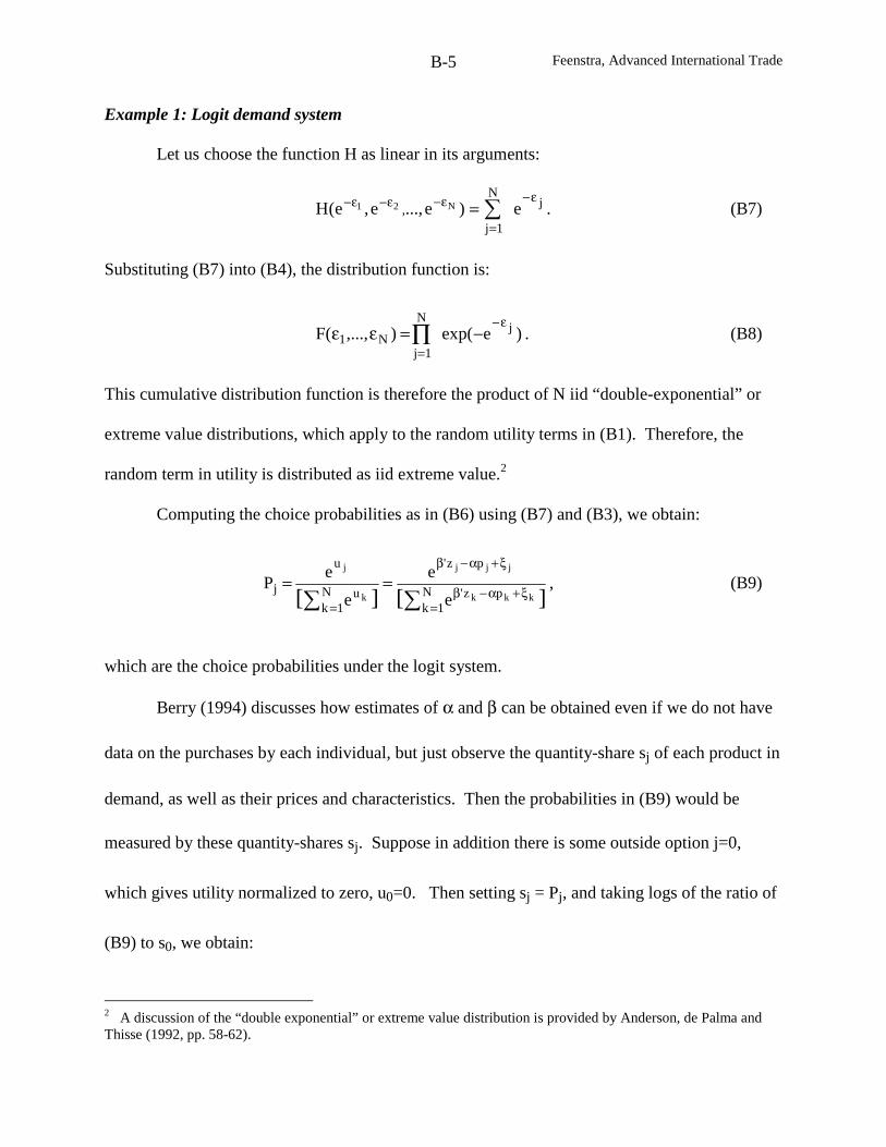
Feenstra, Advanced International TradeB-5
Example 1: Logit demand system
Let us choose the function H as linear in its arguments:
=ε−ε−ε− )e...,e,e(H N21 ,j
N
1j
eε−
=∑ . (B7)
Substituting (B7) into (B4), the distribution function is:
)eexp(),...,(F jN
1jN1
ε−
=−=εε ∏ . (B8)
This cumulative distribution function is therefore the product of N iid “double-exponential” or
extreme value distributions, which apply to the random utility terms in (B1). Therefore, the
random term in utility is distributed as iid extreme value.2
Computing the choice probabilities as in (B6) using (B7) and (B3), we obtain:
][][ N1k
pz'
pz'
N1k
u
u
jkkk
jjj
k
j
e
e
e
eP
∑∑ =ξ+α−β
ξ+α−β
=
== , (B9)
which are the choice probabilities under the logit system.
Berry (1994) discusses how estimates of α and β can be obtained even if we do not have
data on the purchases by each individual, but just observe the quantity-share sj of each product in
demand, as well as their prices and characteristics. Then the probabilities in (B9) would be
measured by these quantity-shares sj. Suppose in addition there is some outside option j=0,
which gives utility normalized to zero, u0=0. Then setting sj = Pj, and taking logs of the ratio of
(B9) to s0, we obtain:
2 A discussion of the “double exponential” or extreme value distribution is provided by Anderson, de Palma andThisse (1992, pp. 58-62).
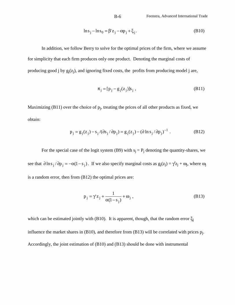
Feenstra, Advanced International TradeB-6
jjj0j pz'slnsln ξ+α−β=− . (B10)
In addition, we follow Berry to solve for the optimal prices of the firm, where we assume
for simplicity that each firm produces only one product. Denoting the marginal costs of
producing good j by gj(zj), and ignoring fixed costs, the profits from producing model j are,
jjjjj s)]z(gp[ −=π , (B11)
Maximizing (B11) over the choice of pj, treating the prices of all other products as fixed, we
obtain:
1jjjjjjjjjj )p/sln()z(g)p/s/(s)z(gp −∂∂−=∂∂−= . (B12)
For the special case of the logit system (B9) with sj = Pj denoting the quantity-shares, we
see that )s1(p/sln jjj −α−=∂∂ . If we also specify marginal costs as gj(zj) = γ’zj + ωj, where ωj
is a random error, then from (B12) the optimal prices are:
jj
jj )s1(
1z'p ω+
−α+γ= , (B13)
which can be estimated jointly with (B10). It is apparent, though, that the random error ξj
influence the market shares in (B10), and therefore from (B13) will be correlated with prices pj.
Accordingly, the joint estimation of (B10) and (B13) should be done with instrumental
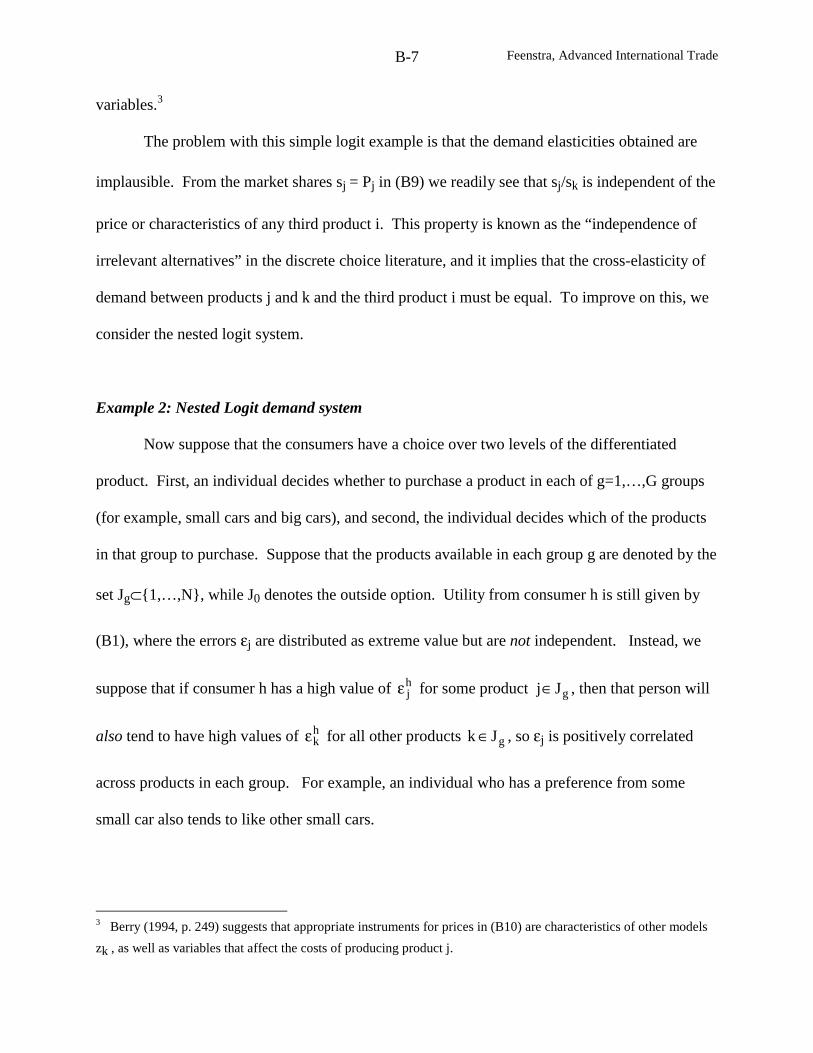
Feenstra, Advanced International TradeB-7
variables.3
The problem with this simple logit example is that the demand elasticities obtained are
implausible. From the market shares sj = Pj in (B9) we readily see that sj/sk is independent of the
price or characteristics of any third product i. This property is known as the “independence of
irrelevant alternatives” in the discrete choice literature, and it implies that the cross-elasticity of
demand between products j and k and the third product i must be equal. To improve on this, we
consider the nested logit system.
Example 2: Nested Logit demand system
Now suppose that the consumers have a choice over two levels of the differentiated
product. First, an individual decides whether to purchase a product in each of g=1,…,G groups
(for example, small cars and big cars), and second, the individual decides which of the products
in that group to purchase. Suppose that the products available in each group g are denoted by the
set Jg⊂{1,…,N}, while J0 denotes the outside option. Utility from consumer h is still given by
(B1), where the errors εj are distributed as extreme value but are not independent. Instead, we
suppose that if consumer h has a high value of hjε for some product gJj∈ , then that person will
also tend to have high values of hkε for all other products gJk ∈ , so εj is positively correlated
across products in each group. For example, an individual who has a preference from some
small car also tends to like other small cars.
3 Berry (1994, p. 249) suggests that appropriate instruments for prices in (B10) are characteristics of other models
zk , as well as variables that affect the costs of producing product j.
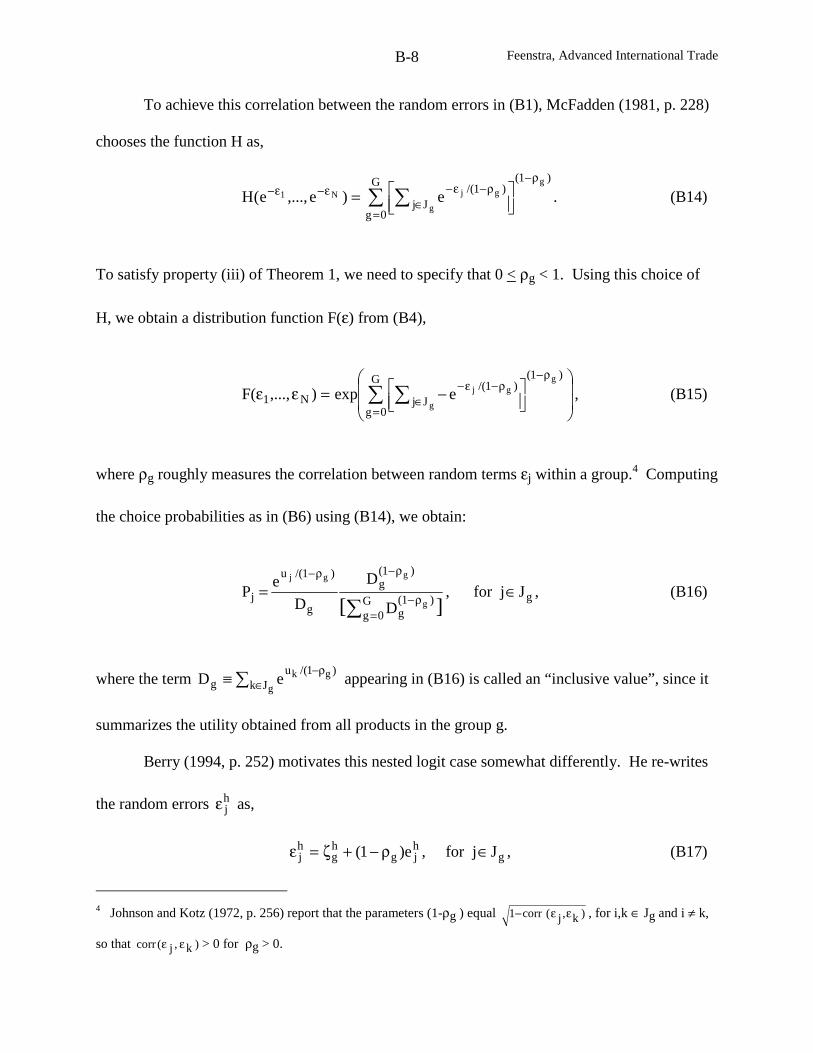
Feenstra, Advanced International TradeB-8
To achieve this correlation between the random errors in (B1), McFadden (1981, p. 228)
chooses the function H as,
=ε−ε− )e,...,e(H N1
)1(G
0gJj
)1/(g
g
gjeρ−
=∈
ρ−ε−∑ ∑
. (B14)
To satisfy property (iii) of Theorem 1, we need to specify that 0 < ρg < 1. Using this choice of
H, we obtain a distribution function F(ε) from (B4),
=εε ),...,(F N1
−
ρ−
=∈
ρ−ε−∑ ∑)1(G
0gJj
)1/(g
g
gjeexp , (B15)
where ρg roughly measures the correlation between random terms εj within a group.4 Computing
the choice probabilities as in (B6) using (B14), we obtain:
∑ =ρ−
ρ−ρ−=
G0g
)1(g
)1(g
g
)1/(u
j][ g
ggj
D
D
D
eP , for gJj∈ , (B16)
where the term ∑ ∈ρ−≡
g
gkJk
)1/(ug eD appearing in (B16) is called an “inclusive value”, since it
summarizes the utility obtained from all products in the group g.
Berry (1994, p. 252) motivates this nested logit case somewhat differently. He re-writes
the random errors hjε as,
hjg
hg
hj e)1( ρ−+ζ=ε , for gJj∈ , (B17)
4 Johnson and Kotz (1972, p. 256) report that the parameters (1-ρg ) equal )k,j(corr1 εε− , for i,k ∈ Jg and i ≠ k,
so that )k,j(corr εε > 0 for ρg > 0.
Feenstra, Advanced International TradeB-9
where the errors hje are iid extreme value. The random variable h
gζ in (B17) is common to all
products within group g, and therefore induces a correlation between the random utilities for
those products. Cardell (1997) shows that there exists a distribution for hgζ (depending on ρg)
such that when hje are iid extreme value, then h
jε are also distributed extreme value but are not
independent. Notice that as the parameter ρg approaches unity then hjε are perfectly correlated
within the group g (since they equal hgζ ), whereas when ρg approaches zero (in which case h
gζ
also approaches zero) then hjε become independent. Using the errors in (B17) gives the same
choice probabilities as shown in (B16).
Using the nested logit choice probabilities in (B16), we can re-derive the estimating
equations for market share and optimal prices, as in Berry (1994, pp. 252-253). The first term on
the right of (B16) is the probability that an individual will choose product gJj∈ conditional on
having already chosen the group g. Let us denote this conditional probability by g|js . The
second term on the right of (B16) is the probability of choosing any product from group g, which
we write as gs . So replacing Pj in (B16) by the market shares sj, we write this choice probability
as gg|jj sss = . In addition, we suppose that the outside good has u0=0 and inclusive value D0=1,
so that from (B16),1G
0g)1(
g00 ][ gDPs−
=ρ−∑== . Taking logs of the ratio 0gg|j0j s/sss/s = and
using the linear utility uj in (B3), we therefore have,
Feenstra, Advanced International TradeB-10
ggg
jjj0j Dln
)1(
)pz'(slnsln ρ−
ρ−ξ+α−β
=− . (B18)
To solve for the inclusive value Dg, recall that gs equals the second term on the right of
(B16). Therefore,)1(
g0ggDs/s
ρ−= and so gg0g Dln)1(slnsln ρ−=− . Using this in (B18) and
simplifying with gg|jj sss = , we obtain,
jg|jgjj0j slnpz'slnsln ξ+ρ+α−β=− , gJj∈ . (B19)
This gives us a regression to estimate the parameters (α,β), where the final term g|jsln measures
the market share of product j within the group g, and is endogenous. Once again, we can use
instrumental variables to estimate (B19).5
In addition, we follow Berry (1994, p. 255) to solve for the optimal prices of the firm,
assuming for simplicity that it produces only one product j. Profits are still given by (B11), and
the first-order condition by (B12). For the nested logit system with sj = Pj in (B16), the
derivative of the log market shares is ]s)1(s1[)1(
p/sln jgg|jgg
jj ρ−−σ−σ−α−=∂∂ . With
marginal costs as gj(zj) = γ’zj + ωj, where ωj is a random error, from (B11) the optimal prices are:
jjgg|jg
gjj ]s)1(s1[
)1(z'p ω+
ρ−−ρ−αρ−
+γ= , (B20)
5 Berry (1994, p. 254) suggests that appropriate instruments will include the characteristics of other products orfirms in group g.
Feenstra, Advanced International TradeB-11
which can be estimated simultaneously with (B19) using instrumental variables. This pricing
equation was generalized in chapter 8 to allow for multi-product firms, as used by Irwin and
Pavcnik (2001) in their study of export subsidies to commercial aircraft.
The nested logit allows for more general substitution between products than does the
simple logit model (and does not suffer from “independence of irrelevant alternatives”).
Goldberg (1995), for example, has used the nested logit in her study of automobile demand in the
U.S. and the impact of the voluntary export restraint (VER) with Japan. Nevertheless, more
flexible in the pattern of demand across autos can be achieved by introducing greater consumer
heterogeneity, as done by Berry, Levinsohn and Pakes (1993, 1999) in their work on autos and
the VER with Japan. They suppose that the utilities in (B3) instead appear as,
jjjhh
j pz'u ξ++α−β= , α > 0, (B3’)
where now the parameters βhdepend on the individual h, reflecting both demographic
characteristics and income. Since individual income is included in βh, without loss of generality
we omit this variable from appearing explicitly in (B3’).
If we observed both individual characteristics and also their discrete choices, then it
would be possible to estimate the other parameters appearing in (B3’) using standard
econometric programs for discrete choice. However, when we observe only the market-level
demands and overall distribution of individual characteristics, then estimating the parameters of
(B3’) becomes much more difficult. To see this, let us suppose that the individual characteristics
βhare distributed as hη+β , with mean value β over the population and hη is a random
variable that captures individual tastes for characteristics. Substituting this into (B3’) and then
into (B1), we obtain utility,
Feenstra, Advanced International TradeB-12
)z'(pz'V hjj
hjjj
hj ε+η+ξ+α−β= , (B1’)
where now the random error includes the interaction term jh z'η between individual tastes and
product characteristics. The presence of this interaction term means that Theorem 1 cannot be
used: the cumulative distribution of the combined error )z'( hjj
h ε+η is more general than
allowed for in Theorem 1. It follows that there is no closed-form solution such as (B6) for the
choice probabilities.
Instead, the choice probabilities need to be calculated numerically from (B2). That is,
given the data (pj,zj) across products we can simulate the distribution of )z'( hjj
h ε+η . For each
draw from this distribution, and for given parameters ),,( jξβα , we can calculate utility hjV for
each product. The choice probabilities Pj in (B2) are computed as the proportion of draws for
which product j gives the highest utility. Then the parameters ),,( jξβα are chosen so that these
choice probabilities match the observed market shares sj as closely as possible. Likewise, the
predicted change in the market shares due to prices, )p/s( jj ∂∂ in (B12), would be calculated
numerically by seeing how the choice probability Pj vary with prices pj. This also depends on
the parameters ),,( jξβα , which are then chosen so that the pricing equations fit as closely as
possible. Thus, the market share and pricing equations are simultaneously used to estimate the
underlying taste and costs parameters, using simulated distributions of the random term in utility.
This is the idea behind the work of Berry, Levinsohn and Pakes (1993, 1999), to which you are
Feenstra, Advanced International TradeB-13
referred for more details.6
It is also useful to compare the above approaches with a third approach to discrete choice
models: rather than using a representative consumer, or individuals with random utility, we
could instead use individuals that differ in terms of their preferred characteristics, in what is
sometimes called the “ideal variety” approach. Anderson, de Palma and Thisse (1992) derive an
equivalence between all three approaches. Bresnahan (1981) was the first to estimate a discrete
choice model for autos in which consumers differ in their ideal varieties, and found that higher-
priced models tended to have higher percentage markups. Feenstra and Levinsohn (1995)
generalized the model of Bresnahan by allowing characteristics to differ multi-dimensionally,
rather than along a line as in Bresnahan, and show how the optimal prices of firms will vary with
the distance to their nearest neighbors.
Discrete Choice with Continuous Quantities
Setting aside the issue of consumer heterogeneity, there is another direction in which we
can attempt to generalize Theorem 1, while still allowing the aggregate utility function to exist so
that demands can be computed using Roy’s Identity. We again suppose that consumers are still
choosing over products j=1,…,N, and now have the utility function:
hjV = ln y – )z,p(ln jjφ + h
jε , j=1,…,N, (B21)
where pj is the price of product j, zj is a vector of characteristics, y is the consumers’ income, and
εj is a random term that reflects the additional utility received by consumer h from product j.
6 Estimating a discrete choice model by simulating the taste parameters is referred to as “mixed logit”. See, forexample, McFadden and Train (1997) and Revelt and Train (1999). A distance learning course on discrete choicemethods including software to estimate mixed logit models is available from Kenneth Train athttp://elsa.berkeley.edu/~train/distant.html.
Feenstra, Advanced International TradeB-14
Thus, income no longer enter utility in a linear fashion, and we will allow individuals to consume
continuous quantities (not restricted to 0 or 1) of their preferred product j.
Each consumer still chooses their preferred product j with probability:
Pj = Prob[Vj > Vk for all k=1,…,N ] . (B22)
If product j is chosen, then the quantity consumed is determined from the indirect utility function
in (B21), using Roy’s identity:
cj =y/V
p/Vhj
jhj
∂∂
∂∂− = y )jp/ln( ∂φ∂ . (B23)
It follows that expected demand for each product is:
Xj = cjPj . (B24)
This formulation of the consumer’s problem is somewhat more general than what we
considered earlier, because now we are allowing the consumer to make a continuous choice of
the quantity purchased. This falls into the category of so-called “continuous/discrete” models
(see Train, 1986, chap. 5). However, our formulation of the problem is simplified, however,
because there is no uncertainty over the quantity of purchases in (B24); the random term in
utility affects only the choice of product in (B22).7 It turns out that in this setting, the
aggregation results of McFadden (1978, 1981) apply equally well, and we can extend Theorem 1
as: 8
7 In contrast, Dubin and McFadden (1984) consider an application where there is uncertainty in both the discretechoice of the product and the continuous amount to consume.8 The proof of Theorem 2, based on the results of McFadden, is provided in Feenstra (1995, Prop. 1).
Feenstra, Advanced International TradeB-15
Theorem 2
Let H be a nonnegative function defined over NR + that satisfies conditions (i)-(iii) of Theorem 1.
Define the cumulative distribution function F as in (B3), and define an aggregate indirect utility
function,
]1NN
111NN11 )z,p(,...,)z,p([Hlnyln)y,z,p,...,z,p(G −− φφ+= . (B25)
Then:
(a) Expected demand computed from (B24) equals )y/G/()p/G( j ∂∂∂∂− ;
(b) G equals expected individual utility in (B21) (up to a constant).
Thus, we can still compute demand using Roy’s identity as in part (a), and use the
aggregate utility function to infer welfare as in part (b). Notice that expected utility can be re-
written in a more familiar form by taking the monotonic transformation )Gexp(G~ = , so that,
]1NN
111NN11 )z,p(,...,)z,p([Hy)y,z,p,...,z,p(G
~ −− φφ= . (B25’)
This can be interpreted as an indirect utility function for the representative consumer.
To see the usefulness of this result, we consider again a random utility εj in (B21) that are
independently distributed across products, with the extreme value distribution, and derive a CES
aggregate utility function.
Feenstra, Advanced International TradeB-16
Example 3: CES demand system
Let us specify the individual utility functions as: 9
hjV = ln y – αln[pj/f(zj)] + h
jε , α > 0, (B26)
where we are measuring prices relative to consumers’ perceived “quality” of products f(zj).
We will choose the function H as linear in its arguments, as in (B7). It follows that the
cumulative distribution function in (B8) is the product of N iid extreme value distributions, so
the errors in (B26) are distributed as iid extreme value.
Then using (B7), (B25) and (B26), we obtain the aggregate utility function as:
=)y,z,p,...,z,p(G NN11 ∑=
α−N
1jjj )]z(f/p[y , (B27)
so that expected aggregate demand is,
α=
∂∂∂∂
−∑ =
α−
−α−
N1k kk
1jjj
)]z(f/p[
)]z(f/p[y
y/G
p/G. (B28)
Thus, we obtain a CES indirect utility function in (B27) for the aggregate consumer, with
elasticity of substitution with σ = 1+α, and the associated CES demand in (B28). This is an
alternative demonstration of the result in Anderson, de Palma and Thisse (1989; 1992, pp. 85-
90), that the CES utility function arrives from a discrete choice model with iid extreme value
errors in random utility. Notice that this CES demand system is obtained with exactly the same
9 This utility function is not homogeneous of degree zero in income y and price pj. To obtain this property, we
should measure y and pj relative to a numeraire price p0, so that utility becomes ln(y/p0) – αln[(pj/p0)/f(zj)], which
is homogeneous of degree zero in (y, pj, p0).
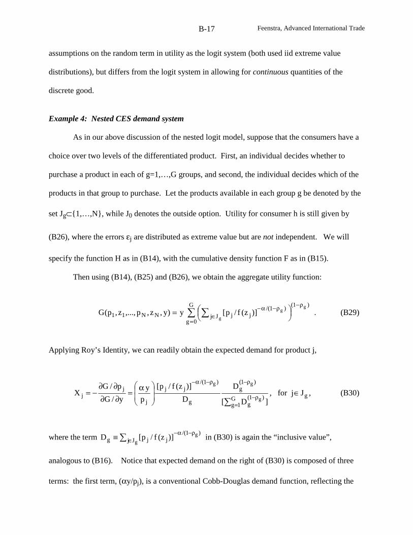
Feenstra, Advanced International TradeB-17
assumptions on the random term in utility as the logit system (both used iid extreme value
distributions), but differs from the logit system in allowing for continuous quantities of the
discrete good.
Example 4: Nested CES demand system
As in our above discussion of the nested logit model, suppose that the consumers have a
choice over two levels of the differentiated product. First, an individual decides whether to
purchase a product in each of g=1,…,G groups, and second, the individual decides which of the
products in that group to purchase. Let the products available in each group g be denoted by the
set Jg⊂{1,…,N}, while J0 denotes the outside option. Utility for consumer h is still given by
(B26), where the errors εj are distributed as extreme value but are not independent. We will
specify the function H as in (B14), with the cumulative density function F as in (B15).
Then using (B14), (B25) and (B26), we obtain the aggregate utility function:
=)y,z,p,...,z,p(G NN11 ∑ ∑=
ρ−
∈ρ−α−
G
0g
)1(
Jj)1/(
jj
g
g
g)]z(f/p[y . (B29)
Applying Roy’s Identity, we can readily obtain the expected demand for product j,
∑ =ρ−
ρ−ρ−α−
α=∂∂∂∂
−=G
1g)1(
g
)1(g
g
)1/(jj
j
jj
]D[
D
D
)]z(f/p[
p
y
y/G
p/GX
g
gg
, for gJj∈ , (B30)
where the term ∑ ∈ρ−α−≡
gg
Jj)1/(
jjg )]z(f/p[D in (B30) is again the “inclusive value”,
analogous to (B16). Notice that expected demand on the right of (B30) is composed of three
terms: the first term, (αy/pj), is a conventional Cobb-Douglas demand function, reflecting the
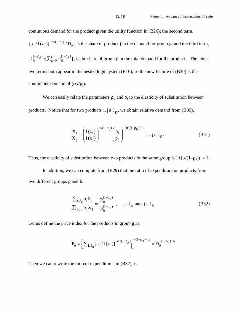
Feenstra, Advanced International TradeB-18
continuous demand for the product given the utility function in (B26); the second term,
g)1/(
jj D/)]z(f/p[ iρ−α− , is the share of product j in the demand for group g; and the third term,
∑ =ρ−ρ− G
0g)1(
g)1(
g ]D/[D gg , is the share of group g in the total demand for the product. The latter
two terms both appear in the nested logit system (B16), so the new feature of (B30) is the
continuous demand of (αy/pj).
We can easily relate the parameters ρ0 and ρi to the elasticity of substitution between
products. Notice that for two products gJj,i ∈ , we obtain relative demand from (B30),
1)]1/([
j
i
)1/(
j
i
j
igg
p
p
)z(f
)z(f
X
X−ρ−α−ρ−α
= , gJj,i ∈ . (B31)
Thus, the elasticity of substitution between two products in the same group is 1+[α/(1–ρg )] > 1.
In addition, we can compute from (B29) that the ratio of expenditure on products from
two different groups g and h:
)1(h
)1(g
jJj j
iJi i
h
g
h
g
D
D
Xp
Xp
ρ−
ρ−
∈
∈=
∑
∑, hg JjandJi ∈∈ . (B32)
Let us define the price index for the products in group g as,
αρ−−αρ−−
∈ρ−α− =
≡ ∑
/)1(g
/)1(
Jj)1/(
jjggg
gg D)]z(f/p[P .
Then we can rewrite the ratio of expenditures in (B32) as,
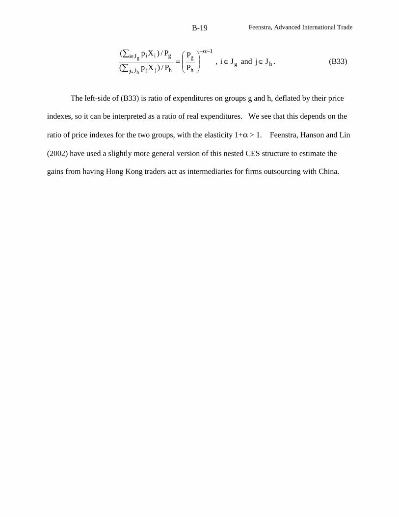
Feenstra, Advanced International TradeB-19
1
h
g
hjJj j
giJi i
P
P
P/)Xp(
P/)Xp(
h
g−α−
∈
∈
=
∑
∑, hg JjandJi ∈∈ . (B33)
The left-side of (B33) is ratio of expenditures on groups g and h, deflated by their price
indexes, so it can be interpreted as a ratio of real expenditures. We see that this depends on the
ratio of price indexes for the two groups, with the elasticity 1+α > 1. Feenstra, Hanson and Lin
(2002) have used a slightly more general version of this nested CES structure to estimate the
gains from having Hong Kong traders act as intermediaries for firms outsourcing with China.
References
Abiru, Masahiro, Babu Nahata, Subhashis Raychaudhuri, and Michael Waterson, 1998,
“Equilibrium Structure in Vertical Oligopoly,” Journal of Economic Behavior and
Organization, 37, 463-480.
Acemoglu, Daron and Jaume Ventura, 2002, “The World Income Distribution,”
Quarterly Journal of Economics, 117(2), 659-694.
Acemoglu, Daron, Simon Johnson and James A. Robinson, 2001, “The Colonial Origins
of Comparative Development: An Empirical Investigation,” American Economic
Review, 91(5), December, 1369-1401.
Aghion, Phillipe and Jean Tirole, “Formal and Real Authority in Organizations,” Journal
of Political Economy, 105(1), 1-29.
Aho, C. Michael and Thomas O. Bayard, 1984, “Costs and Benefits of Trade Adjustment
Assistance,” in Robert E. Baldwin and Anne O. Krueger, eds. The Structure and
Evolution of Recent U.S. Trade Policy. Chicago: Univ. of Chicago and NBER,
153-192.
Aitken, Brian, and Ann E. Harrison, 1999, “Do Domestic Firms Benefit from Foreign
Investment? Evidence from Venezuela,” American Economic Review, 89, 605-
618.
Aitken, Brian, Ann E. Harrison, and Robert Lipsey, 1996, “Wages and Foreign
Ownership: A Comparative Study of Mexico, Venezuela, and the United States,”
Journal of International Economics, 40(3/4), 345-371.
Akerlof, George, Andrew Rose, Janet Yellen and Helga Hessenius, 1991, “East Germany
in from the Cold: The Economic Aftermath of Currency Union,” Brookings
Papers on Economic Activity, vol. 1.
Alchian, Armen A. and William R. Allen, 1964, University Economics, Belmont, CA:
Wadsworth, 1964 and later editions.
Alesina, Alberto and Dani Rodrik, 1994, “Distribute Politics and Economic Growth,”
Quarterly Journal of Economics, May, 109(2), 465-490.
R-2
Alterman, William F., W. Erwin Diewert, and Robert C. Feenstra, 1999, International
Trade Price Indexes and Seasonal Commodities. U.S. Dept. of Labor, Bureau of
Labor Statistics, Washington, D.C.
Anderson, James. A., 1979, “A Theoretical Foundation for the Gravity Equation,”
American Economic Review, 69, 106-116.
Anderson, James A., 1985, “The Relative Inefficiency of Quotas: The Cheese Case,”
American Economic Review, 75(1), March, 178-190.
Anderson, James A., 1988, The Relative Inefficiency of Quotas, Cambridge: MIT Press.
Anderson James A. and J. Peter Neary, 1996, “A New Approach to Evaluating Trade
Policy,” Review of Economic Studies, 63, February, 107-125.
Anderson, James A. and Eric van Wincoop, 2001, “Gravity with Gravitas: A Solution to
the Border Puzzle,” NBER Working paper no. 8079.
Anderson, Simon P., Andre de Palma, and Jacques-Francois Thisse, 1992, Discrete
Choice Theory of Product Differentiation, Cambridge, MA: MIT Press.
Anderton, Bob and Paul Brenton, 1999, “Outsourcing and Low-Skilled Workers in the
UK,” Bulletin of Economic Research, 51(4), 267-285.
Antràs, Pol, 2002, “Firms, Contracts and Trade Structure,” Department of Economics,
MIT, manuscript.
Antweiler, Werner and Daniel Trefler, 2002, “Increasing Returns and All That: A View
from Trade,” American Economic Review, 92(1), March, 93-119.
Archibald, R.B., 1977, “On the Theory of Industrial Price Measurement: Output Price
Indexes”, Annals of Economic and Social Measurement 6, 6, 57-62.
Armington, Paul S, 1969, “A Theory of Demand for Products Distinguished by Place and
Production,” IMF Staff Papers, 16, 159-178.
Arndt, Sven, 1998a, “Globalization and the Gains from Trade,” in K. Jaeger and K.-J.
Koch, eds. Trade, Growth and Economic Policy in Open Economies. Springer-
Verlag: New York.
Arndt, Sven, 1998b, “Super-Specialization and the Gains from Trade,” Contemporary
Policy Issues, Western Economic Association, forthcoming.
Arndt, Sven and Henryk Kierzkowski, eds., 2001, Fragmentation: New Production and
Trade Patterns in the World Economy, Oxford University Press, Oxford.
R-3
Autor, David, Lawrence F. Katz, and Alan B. Krueger, 1998, “Computing Inequality:
Have Computers Changed the Labor Market?” Quarterly Journal of Economics,
113(4), 1169-1213.
Aw, Bee Yan, 1983, “The Interpretation of Cross-Section Regression Tests of the
Heckscher-Ohlin Theorem with Many Goods and Factors, Journal of
International Economics, 14(1-2), February, 163-67.
Bagwell, Kyle and Robert W. Staiger, 1997, “An Economic Theory of GATT”, American
Economic Review, 89(1), March, 215-248.
Bagwell, Kyle and Robert W. Staiger, 2002, The Economics of the World Trading
System. Cambridge: MIT Press.
Barro, Robert J., 1991, “Economic Growth in a Cross-Section of Countries,” Quarterly
Journal of Economics, 106, 407-443.
Barro, Robert J. and Xavier Salai-i-Martin, 1991, “Convergence Across States and
Regions,” Brookings Papers on Economic Activity, 1, 107-158.
Barro, Robert J. and Xavier Salai-i-Martin, 1992, “Convergence,” Journal of Political
Economy, 100(2), 223-251.
Baier, Scott and Jeffrey H. Bergstrand, 2001, “The Growth of World Trade: Tariffs,
Transport Costs, and Income Similarity,” Journal of International Economics,
53(1), February, 1-27.
Baier, Scott and Jeffrey H. Bergstrand, 2002, “On the Endogeneity of International Trade
Flows and Free Trade Agreements,” University of Notre Dame, manuscript.
Baldwin, Richard E., 1995, “A Domino Theory of Regionalism,” in Richard E. Baldwin,
P. Haaparanta and J. Kiander, eds. Expending Membership in the European
Union. Cambridge, UK: Cambridge university Press, 25-48.
Baldwin, Richard E. and Paul R. Krugman, 1988a, “Market Access and International
Competition: A Simulation Study of 16K Random Access Memories,” in Robert
C. Feenstra, ed. Empirical Methods for International Trade. Cambridge: MIT
Press. Reprinted as chapter 10 in Gene M. Grossman, 1992, Imperfect
Competition and International Trade. Cambridge: MIT Press, 177-200.
Baldwin, Richard and Paul Krugman, 1988b, “Industrial Policy and International
Competition in Wide-Bodied Aircraft,” in Robert E. Baldwin, ed. Trade Policy
R-4
Issues and Empirical Analysis. Chicago: University of Chicago and NBER, 45-
71.
Baldwin, Robert E. and Hilton, R.S., 1984, “A Technique for Indicating Comparative
Costs and Predicting Changes in Trade Ratios,” Review of Economics and
Statistics, 64, 105-110.
Baldwin, Robert E., 1969, “The Case Against Infant-Industry Protection,” Journal of
Political Economy, 77, 295-305.
Baldwin, Robert E., 1971, “Determinants of the Commodity Structure of U.S. Trade,”
American Economic Review, March, 61, 126-146.
Baldwin, Robert E. and G.G. Cain, 2000, “Shifts in Relative U.S. Wages: The Role of
Trade, Technology and Factor Endowments,” Review of Economics and Statistics,
82, 580-595.
Bartelsman, Eric J. and Wayne Gray, 1996, “The NBER Manufacturing Productivity
Database,” NBER Technical Working Paper no. 205.
Ben-David, Dan, 1993, “Trade Liberalization and Income Convergence,” Quarterly
Journal of Economics, 108(3), August, 653-679.
Ben-David, Dan, 1998, “Convergence Clubs and Subsistence Economies,” Journal of
Development Economics, 55(1), February, 155-171.
Ben-David, Dan, 2001, “Trade Liberalization and Income Convergence: A Comment,”
Journal of International Economics, 55(1), October, 229-234.�
Benkard, C. Lanier, 2000a, “A Dynamic Analysis of the Market for Wide-Bodied
Commercial Aircraft,” NBER Working Paper #7710, May.
Benkard, C. Lanier, 2000b, “Learning and Forgetting: The Dynamics of Aircraft
Production,” American Economic Review, 90, September, 1034-1054.
Bergin, Paul R. and Robert C. Feenstra, 2000, “Staggered Price Setting and Endogenous
Persistence,” Journal of Monetary Economics, 45, June, 657-680.
Bergin, Paul R. and Robert C. Feenstra, 2001, “Pricing to Market, Staggered Contracts,
and Real Exchange Rate Persistence,” Journal of International Economics, 54(2),
August, 333-359.
R-5
Bergstrand, Jeffrey H., 1985, “The Generalized Gravity Equation, Monopolistic
Competition, and the Factor-Proportions Theory in International Trade,” Review
of Economics and Statistics, 71(1), February, 143-153.
Bergstrand, Jeffrey H., 1989, “The Gravity Equation in International Trade: Some
Microeconomic Foundations and Empirical Evidence,” Review of Economics and
Statistics, 67(3), August, 474-481.
Berman, Eli, John Bound, and Zvi Griliches, 1994, “Changes in the Demand for Skilled
Labor within U.S. Manufacturing: Evidence from the Annual Survey of
Manufactures, Quarterly Journal of Economics, 104, 367-398.
Berman, Eli, John Bound, and Stephen Machin, 1998, “Implications of Skill-Biased
Techno-logical Change: International Evidence,” Quarterly Journal of
Economics, 113,1245-1280.
Bernanke, Ben S. and Refet S. Gürkaynak, 2001, “Is Growth Exogenous? Taking
Mankiw, Romer and Weil Seriously,” in Ben S. Bernanke and Kenneth Rogoff,
eds., NBER Macroeconomics Annual, 2001. Cambridge: MIT Press, 11-57.
Bernard, Andrew B. and J. Bradford Jensen, 1997, “Exporters, Skill Upgrading, and the
Wage Gap,” Journal of International Economics, 42(1/2), February, 3-32.
Bernard, Andrew B. and J. Bradford Jensen, 2000, “Understanding Increasing and
Decreasing Wage Inequality,” in Robert C. Feenstra, ed. The Impact of
International Trade on Wages. Chicago: Univ. of Chicago and NBER, 227-268.
Bernheim, B. Douglas and Michael D. Whinston, 1986, “Menu Auctions, Resource
Allocation, and Economic Influence,” Quarterly Journal of Economics, 101, 1-31.
Bernhofen, Daniel M. and John C. Brown, 2001, “A Direct Test of the Theory of
Comparative Advantage: The case of Japan,” August, Clark University,
manuscript.
Bernstein, Jeffrey R. and David E. Weinstein, 2002, “Do Endowments Predict the
Location of Production? Evidence from National and International Data,” Journal
of International Economics, 56(1), January, 55-76.
Berry, Steven T., 1994, “Estimating Discrete-Choice Models of Product Differentiation,”
Rand Journal of Economics, 25(2), Summer, 242-6.
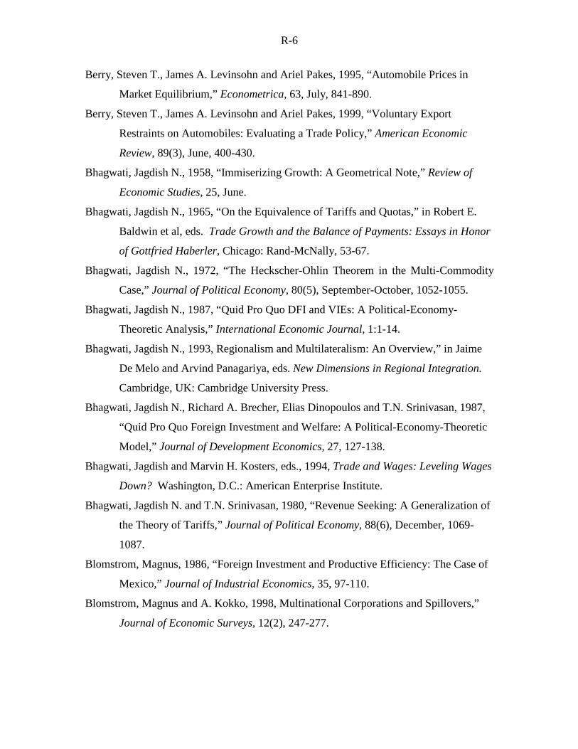
R-6
Berry, Steven T., James A. Levinsohn and Ariel Pakes, 1995, “Automobile Prices in
Market Equilibrium,” Econometrica, 63, July, 841-890.
Berry, Steven T., James A. Levinsohn and Ariel Pakes, 1999, “Voluntary Export
Restraints on Automobiles: Evaluating a Trade Policy,” American Economic
Review, 89(3), June, 400-430.
Bhagwati, Jagdish N., 1958, “Immiserizing Growth: A Geometrical Note,” Review of
Economic Studies, 25, June.
Bhagwati, Jagdish N., 1965, “On the Equivalence of Tariffs and Quotas,” in Robert E.
Baldwin et al, eds. Trade Growth and the Balance of Payments: Essays in Honor
of Gottfried Haberler, Chicago: Rand-McNally, 53-67.
Bhagwati, Jagdish N., 1972, “The Heckscher-Ohlin Theorem in the Multi-Commodity
Case,” Journal of Political Economy, 80(5), September-October, 1052-1055.
Bhagwati, Jagdish N., 1987, “Quid Pro Quo DFI and VIEs: A Political-Economy-
Theoretic Analysis,” International Economic Journal, 1:1-14.
Bhagwati, Jagdish N., 1993, Regionalism and Multilateralism: An Overview,” in Jaime
De Melo and Arvind Panagariya, eds. New Dimensions in Regional Integration.
Cambridge, UK: Cambridge University Press.
Bhagwati, Jagdish N., Richard A. Brecher, Elias Dinopoulos and T.N. Srinivasan, 1987,
“Quid Pro Quo Foreign Investment and Welfare: A Political-Economy-Theoretic
Model,” Journal of Development Economics, 27, 127-138.
Bhagwati, Jagdish and Marvin H. Kosters, eds., 1994, Trade and Wages: Leveling Wages
Down? Washington, D.C.: American Enterprise Institute.
Bhagwati, Jagdish N. and T.N. Srinivasan, 1980, “Revenue Seeking: A Generalization of
the Theory of Tariffs,” Journal of Political Economy, 88(6), December, 1069-
1087.
Blomstrom, Magnus, 1986, “Foreign Investment and Productive Efficiency: The Case of
Mexico,” Journal of Industrial Economics, 35, 97-110.
Blomstrom, Magnus and A. Kokko, 1998, Multinational Corporations and Spillovers,”
Journal of Economic Surveys, 12(2), 247-277.
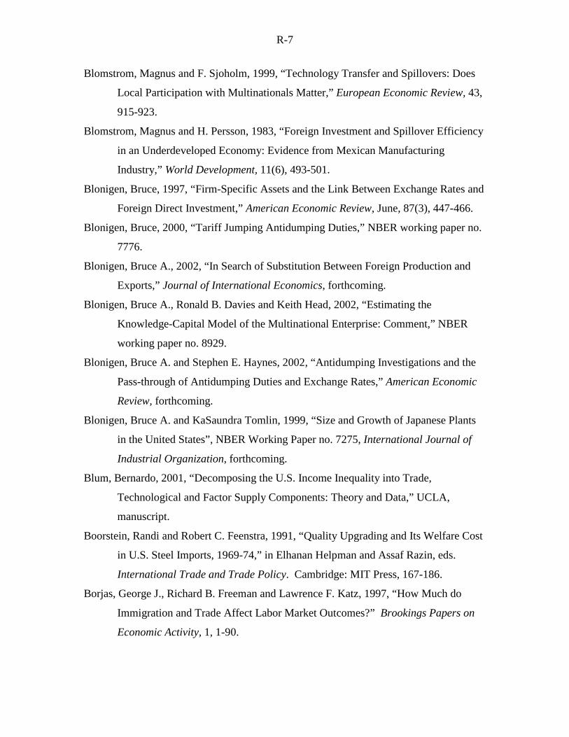
R-7
Blomstrom, Magnus and F. Sjoholm, 1999, “Technology Transfer and Spillovers: Does
Local Participation with Multinationals Matter,” European Economic Review, 43,
915-923.
Blomstrom, Magnus and H. Persson, 1983, “Foreign Investment and Spillover Efficiency
in an Underdeveloped Economy: Evidence from Mexican Manufacturing
Industry,” World Development, 11(6), 493-501.
Blonigen, Bruce, 1997, “Firm-Specific Assets and the Link Between Exchange Rates and
Foreign Direct Investment,” American Economic Review, June, 87(3), 447-466.
Blonigen, Bruce, 2000, “Tariff Jumping Antidumping Duties,” NBER working paper no.
7776.
Blonigen, Bruce A., 2002, “In Search of Substitution Between Foreign Production and
Exports,” Journal of International Economics, forthcoming.
Blonigen, Bruce A., Ronald B. Davies and Keith Head, 2002, “Estimating the
Knowledge-Capital Model of the Multinational Enterprise: Comment,” NBER
working paper no. 8929.
Blonigen, Bruce A. and Stephen E. Haynes, 2002, “Antidumping Investigations and the
Pass-through of Antidumping Duties and Exchange Rates,” American Economic
Review, forthcoming.
Blonigen, Bruce A. and KaSaundra Tomlin, 1999, “Size and Growth of Japanese Plants
in the United States”, NBER Working Paper no. 7275, International Journal of
Industrial Organization, forthcoming.
Blum, Bernardo, 2001, “Decomposing the U.S. Income Inequality into Trade,
Technological and Factor Supply Components: Theory and Data,” UCLA,
manuscript.
Boorstein, Randi and Robert C. Feenstra, 1991, “Quality Upgrading and Its Welfare Cost
in U.S. Steel Imports, 1969-74,” in Elhanan Helpman and Assaf Razin, eds.
International Trade and Trade Policy. Cambridge: MIT Press, 167-186.
Borjas, George J., Richard B. Freeman and Lawrence F. Katz, 1997, “How Much do
Immigration and Trade Affect Labor Market Outcomes?” Brookings Papers on
Economic Activity, 1, 1-90.
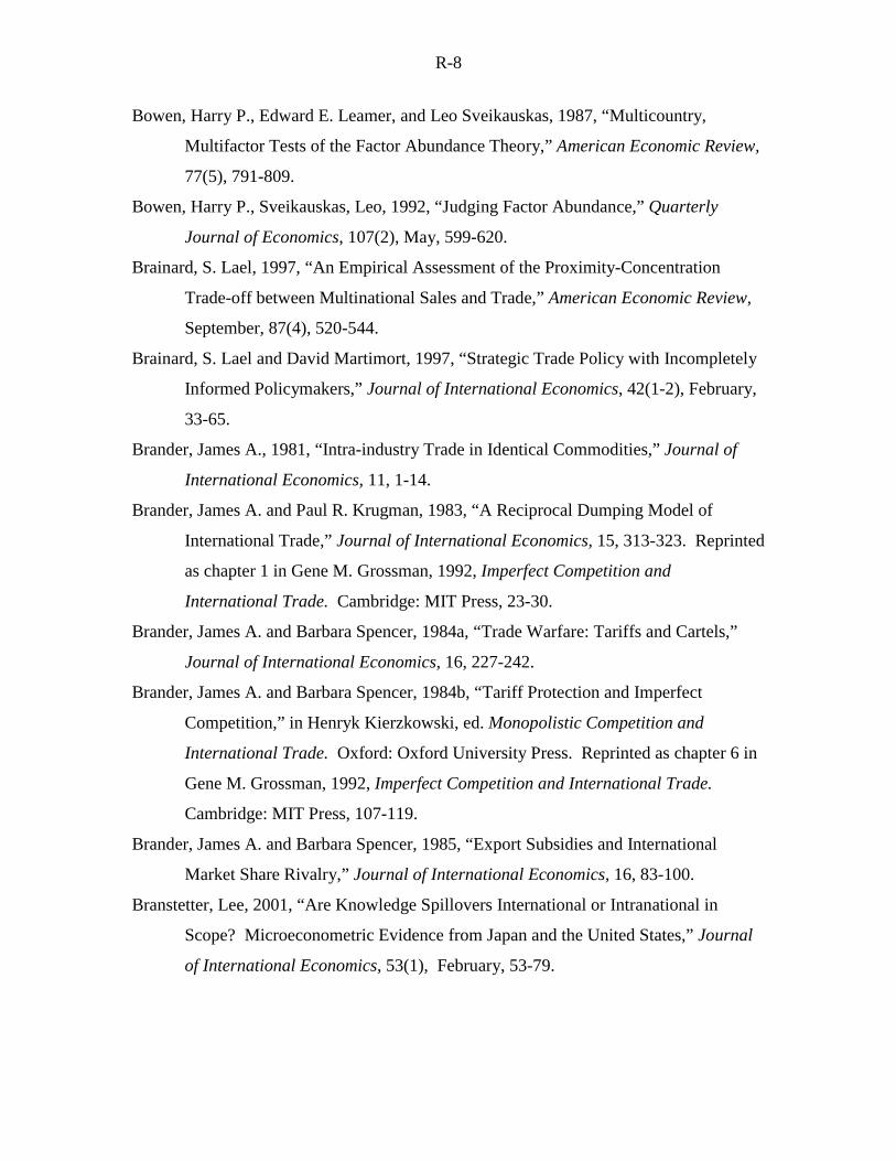
R-8
Bowen, Harry P., Edward E. Leamer, and Leo Sveikauskas, 1987, “Multicountry,
Multifactor Tests of the Factor Abundance Theory,” American Economic Review,
77(5), 791-809.
Bowen, Harry P., Sveikauskas, Leo, 1992, “Judging Factor Abundance,” Quarterly
Journal of Economics, 107(2), May, 599-620.
Brainard, S. Lael, 1997, “An Empirical Assessment of the Proximity-Concentration
Trade-off between Multinational Sales and Trade,” American Economic Review,
September, 87(4), 520-544.
Brainard, S. Lael and David Martimort, 1997, “Strategic Trade Policy with Incompletely
Informed Policymakers,” Journal of International Economics, 42(1-2), February,
33-65.
Brander, James A., 1981, “Intra-industry Trade in Identical Commodities,” Journal of
International Economics, 11, 1-14.
Brander, James A. and Paul R. Krugman, 1983, “A Reciprocal Dumping Model of
International Trade,” Journal of International Economics, 15, 313-323. Reprinted
as chapter 1 in Gene M. Grossman, 1992, Imperfect Competition and
International Trade. Cambridge: MIT Press, 23-30.
Brander, James A. and Barbara Spencer, 1984a, “Trade Warfare: Tariffs and Cartels,”
Journal of International Economics, 16, 227-242.
Brander, James A. and Barbara Spencer, 1984b, “Tariff Protection and Imperfect
Competition,” in Henryk Kierzkowski, ed. Monopolistic Competition and
International Trade. Oxford: Oxford University Press. Reprinted as chapter 6 in
Gene M. Grossman, 1992, Imperfect Competition and International Trade.
Cambridge: MIT Press, 107-119.
Brander, James A. and Barbara Spencer, 1985, “Export Subsidies and International
Market Share Rivalry,” Journal of International Economics, 16, 83-100.
Branstetter, Lee, 2001, “Are Knowledge Spillovers International or Intranational in
Scope? Microeconometric Evidence from Japan and the United States,” Journal
of International Economics, 53(1), February, 53-79.
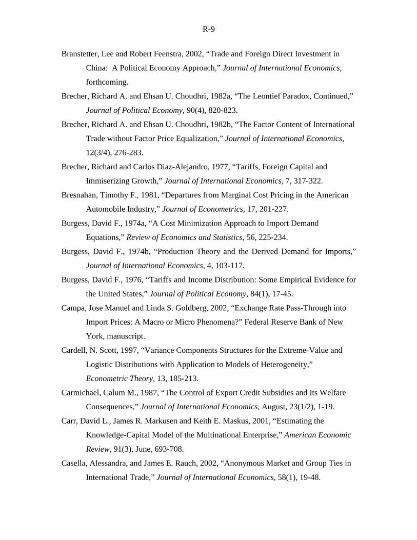
R-9
Branstetter, Lee and Robert Feenstra, 2002, “Trade and Foreign Direct Investment in
China: A Political Economy Approach,” Journal of International Economics,
forthcoming.
Brecher, Richard A. and Ehsan U. Choudhri, 1982a, “The Leontief Paradox, Continued,”
Journal of Political Economy, 90(4), 820-823.
Brecher, Richard A. and Ehsan U. Choudhri, 1982b, “The Factor Content of International
Trade without Factor Price Equalization,” Journal of International Economics,
12(3/4), 276-283.
Brecher, Richard and Carlos Diaz-Alejandro, 1977, “Tariffs, Foreign Capital and
Immiserizing Growth,” Journal of International Economics, 7, 317-322.
Bresnahan, Timothy F., 1981, “Departures from Marginal Cost Pricing in the American
Automobile Industry,” Journal of Econometrics, 17, 201-227.
Burgess, David F., 1974a, “A Cost Minimization Approach to Import Demand
Equations,” Review of Economics and Statistics, 56, 225-234.
Burgess, David F., 1974b, “Production Theory and the Derived Demand for Imports,”
Journal of International Economics, 4, 103-117.
Burgess, David F., 1976, “Tariffs and Income Distribution: Some Empirical Evidence for
the United States,” Journal of Political Economy, 84(1), 17-45.
Campa, Jose Manuel and Linda S. Goldberg, 2002, “Exchange Rate Pass-Through into
Import Prices: A Macro or Micro Phenomena?” Federal Reserve Bank of New
York, manuscript.
Cardell, N. Scott, 1997, “Variance Components Structures for the Extreme-Value and
Logistic Distributions with Application to Models of Heterogeneity,”
Econometric Theory, 13, 185-213.
Carmichael, Calum M., 1987, “The Control of Export Credit Subsidies and Its Welfare
Consequences,” Journal of International Economics, August, 23(1/2), 1-19.
Carr, David L., James R. Markusen and Keith E. Maskus, 2001, “Estimating the
Knowledge-Capital Model of the Multinational Enterprise,” American Economic
Review, 91(3), June, 693-708.
Casella, Alessandra, and James E. Rauch, 2002, “Anonymous Market and Group Ties in
International Trade,” Journal of International Economics, 58(1), 19-48.
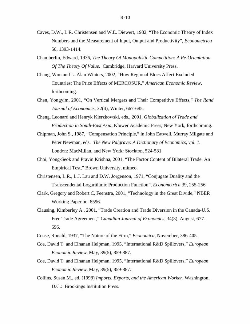
R-10
Caves, D.W., L.R. Christensen and W.E. Diewert, 1982, “The Economic Theory of Index
Numbers and the Measurement of Input, Output and Productivity”, Econometrica
50, 1393-1414.
Chamberlin, Edward, 1936, The Theory Of Monopolistic Competition: A Re-Orientation
Of The Theory Of Value. Cambridge, Harvard University Press.
Chang, Won and L. Alan Winters, 2002, “How Regional Blocs Affect Excluded
Countries: The Price Effects of MERCOSUR,” American Economic Review,
forthcoming.
Chen, Yongyim, 2001, “On Vertical Mergers and Their Competitive Effects,” The Rand
Journal of Economics, 32(4), Winter, 667-685.
Cheng, Leonard and Henryk Kierzkowski, eds., 2001, Globalization of Trade and
Production in South-East Asia, Kluwer Academic Press, New York, forthcoming.
Chipman, John S., 1987, “Compensation Principle,” in John Eatwell, Murray Milgate and
Peter Newman, eds. The New Palgrave: A Dictionary of Economics, vol. 1.
London: MacMillan, and New York: Stockton, 524-531.
Choi, Yong-Seok and Pravin Krishna, 2001, “The Factor Content of Bilateral Trade: An
Empirical Test,” Brown University, mimeo.
Christensen, L.R., L.J. Lau and D.W. Jorgenson, 1971, “Conjugate Duality and the
Transcendental Logarithmic Production Function”, Econometrica 39, 255-256.
Clark, Gregory and Robert C. Feenstra, 2001, “Technology in the Great Divide,” NBER
Working Paper no. 8596.
Clausing, Kimberley A., 2001, “Trade Creation and Trade Diversion in the Canada-U.S.
Free Trade Agreement,” Canadian Journal of Economics, 34(3), August, 677-
696.
Coase, Ronald, 1937, “The Nature of the Firm,” Economica, November, 386-405.
Coe, David T. and Elhanan Helpman, 1995, “International R&D Spillovers,” European
Economic Review, May, 39(5), 859-887.
Coe, David T. and Elhanan Helpman, 1995, “International R&D Spillovers,” European
Economic Review, May, 39(5), 859-887.
Collins, Susan M., ed. (1998) Imports, Exports, and the American Worker, Washington,
D.C.: Brookings Institution Press.
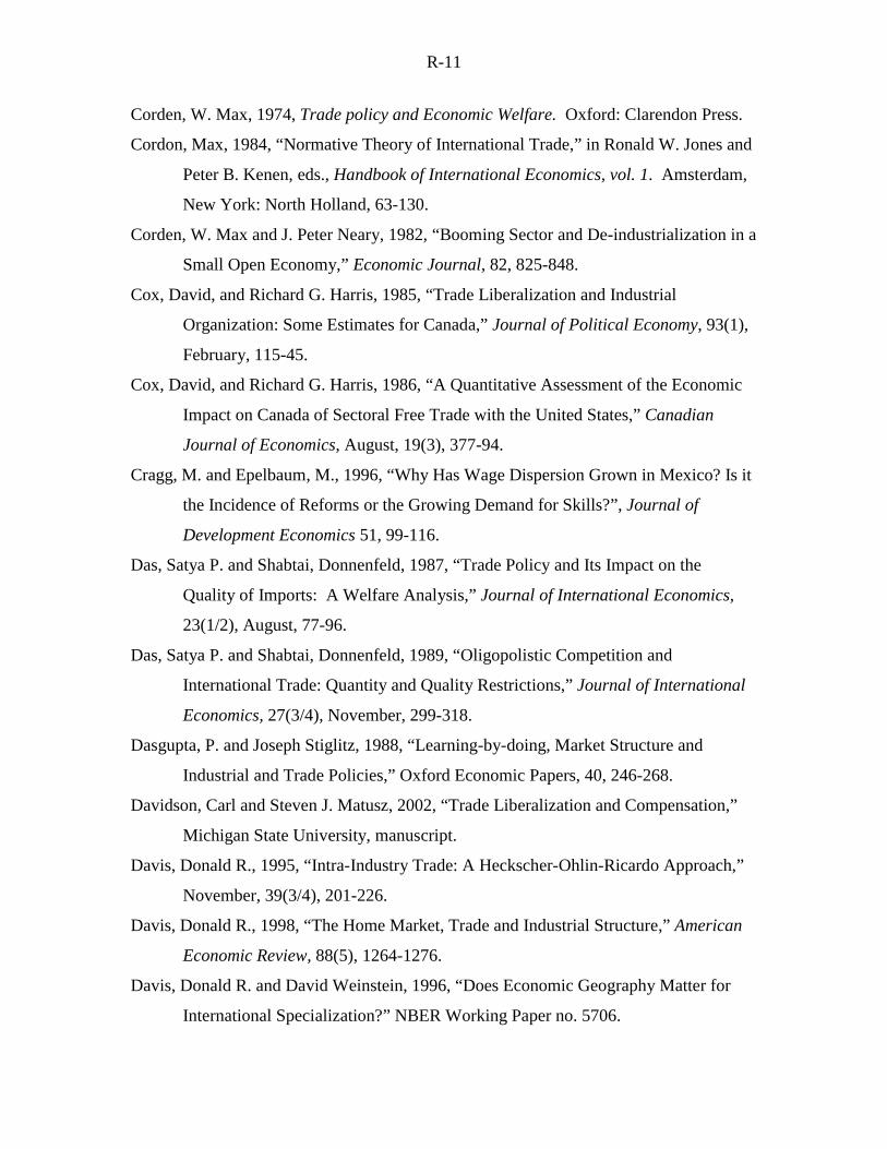
R-11
Corden, W. Max, 1974, Trade policy and Economic Welfare. Oxford: Clarendon Press.
Cordon, Max, 1984, “Normative Theory of International Trade,” in Ronald W. Jones and
Peter B. Kenen, eds., Handbook of International Economics, vol. 1. Amsterdam,
New York: North Holland, 63-130.
Corden, W. Max and J. Peter Neary, 1982, “Booming Sector and De-industrialization in a
Small Open Economy,” Economic Journal, 82, 825-848.
Cox, David, and Richard G. Harris, 1985, “Trade Liberalization and Industrial
Organization: Some Estimates for Canada,” Journal of Political Economy, 93(1),
February, 115-45.
Cox, David, and Richard G. Harris, 1986, “A Quantitative Assessment of the Economic
Impact on Canada of Sectoral Free Trade with the United States,” Canadian
Journal of Economics, August, 19(3), 377-94.
Cragg, M. and Epelbaum, M., 1996, “Why Has Wage Dispersion Grown in Mexico? Is it
the Incidence of Reforms or the Growing Demand for Skills?”, Journal of
Development Economics 51, 99-116.
Das, Satya P. and Shabtai, Donnenfeld, 1987, “Trade Policy and Its Impact on the
Quality of Imports: A Welfare Analysis,” Journal of International Economics,
23(1/2), August, 77-96.
Das, Satya P. and Shabtai, Donnenfeld, 1989, “Oligopolistic Competition and
International Trade: Quantity and Quality Restrictions,” Journal of International
Economics, 27(3/4), November, 299-318.
Dasgupta, P. and Joseph Stiglitz, 1988, “Learning-by-doing, Market Structure and
Industrial and Trade Policies,” Oxford Economic Papers, 40, 246-268.
Davidson, Carl and Steven J. Matusz, 2002, “Trade Liberalization and Compensation,”
Michigan State University, manuscript.
Davis, Donald R., 1995, “Intra-Industry Trade: A Heckscher-Ohlin-Ricardo Approach,”
November, 39(3/4), 201-226.
Davis, Donald R., 1998, “The Home Market, Trade and Industrial Structure,” American
Economic Review, 88(5), 1264-1276.
Davis, Donald R. and David Weinstein, 1996, “Does Economic Geography Matter for
International Specialization?” NBER Working Paper no. 5706.
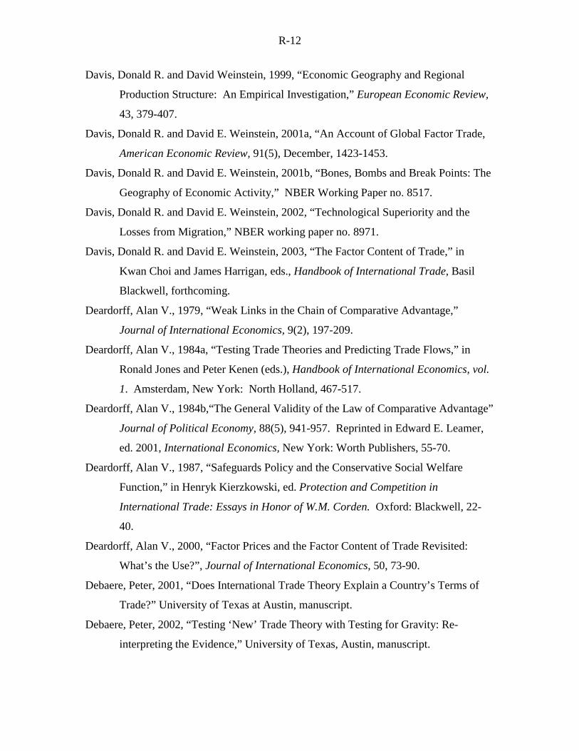
R-12
Davis, Donald R. and David Weinstein, 1999, “Economic Geography and Regional
Production Structure: An Empirical Investigation,” European Economic Review,
43, 379-407.
Davis, Donald R. and David E. Weinstein, 2001a, “An Account of Global Factor Trade,
American Economic Review, 91(5), December, 1423-1453.
Davis, Donald R. and David E. Weinstein, 2001b, “Bones, Bombs and Break Points: The
Geography of Economic Activity,” NBER Working Paper no. 8517.
Davis, Donald R. and David E. Weinstein, 2002, “Technological Superiority and the
Losses from Migration,” NBER working paper no. 8971.
Davis, Donald R. and David E. Weinstein, 2003, “The Factor Content of Trade,” in
Kwan Choi and James Harrigan, eds., Handbook of International Trade, Basil
Blackwell, forthcoming.
Deardorff, Alan V., 1979, “Weak Links in the Chain of Comparative Advantage,”
Journal of International Economics, 9(2), 197-209.
Deardorff, Alan V., 1984a, “Testing Trade Theories and Predicting Trade Flows,” in
Ronald Jones and Peter Kenen (eds.), Handbook of International Economics, vol.
1. Amsterdam, New York: North Holland, 467-517.
Deardorff, Alan V., 1984b,“The General Validity of the Law of Comparative Advantage”
Journal of Political Economy, 88(5), 941-957. Reprinted in Edward E. Leamer,
ed. 2001, International Economics, New York: Worth Publishers, 55-70.
Deardorff, Alan V., 1987, “Safeguards Policy and the Conservative Social Welfare
Function,” in Henryk Kierzkowski, ed. Protection and Competition in
International Trade: Essays in Honor of W.M. Corden. Oxford: Blackwell, 22-
40.
Deardorff, Alan V., 2000, “Factor Prices and the Factor Content of Trade Revisited:
What’s the Use?”, Journal of International Economics, 50, 73-90.
Debaere, Peter, 2001, “Does International Trade Theory Explain a Country’s Terms of
Trade?” University of Texas at Austin, manuscript.
Debaere, Peter, 2002, “Testing ‘New’ Trade Theory with Testing for Gravity: Re-
interpreting the Evidence,” University of Texas, Austin, manuscript.
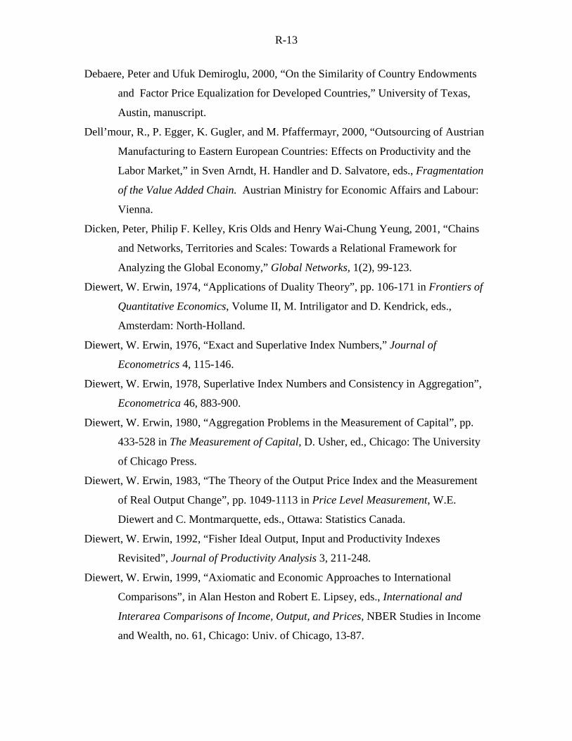
R-13
Debaere, Peter and Ufuk Demiroglu, 2000, “On the Similarity of Country Endowments
and Factor Price Equalization for Developed Countries,” University of Texas,
Austin, manuscript.
Dell’mour, R., P. Egger, K. Gugler, and M. Pfaffermayr, 2000, “Outsourcing of Austrian
Manufacturing to Eastern European Countries: Effects on Productivity and the
Labor Market,” in Sven Arndt, H. Handler and D. Salvatore, eds., Fragmentation
of the Value Added Chain. Austrian Ministry for Economic Affairs and Labour:
Vienna.
Dicken, Peter, Philip F. Kelley, Kris Olds and Henry Wai-Chung Yeung, 2001, “Chains
and Networks, Territories and Scales: Towards a Relational Framework for
Analyzing the Global Economy,” Global Networks, 1(2), 99-123.
Diewert, W. Erwin, 1974, “Applications of Duality Theory”, pp. 106-171 in Frontiers of
Quantitative Economics, Volume II, M. Intriligator and D. Kendrick, eds.,
Amsterdam: North-Holland.
Diewert, W. Erwin, 1976, “Exact and Superlative Index Numbers,” Journal of
Econometrics 4, 115-146.
Diewert, W. Erwin, 1978, Superlative Index Numbers and Consistency in Aggregation”,
Econometrica 46, 883-900.
Diewert, W. Erwin, 1980, “Aggregation Problems in the Measurement of Capital”, pp.
433-528 in The Measurement of Capital, D. Usher, ed., Chicago: The University
of Chicago Press.
Diewert, W. Erwin, 1983, “The Theory of the Output Price Index and the Measurement
of Real Output Change”, pp. 1049-1113 in Price Level Measurement, W.E.
Diewert and C. Montmarquette, eds., Ottawa: Statistics Canada.
Diewert, W. Erwin, 1992, “Fisher Ideal Output, Input and Productivity Indexes
Revisited”, Journal of Productivity Analysis 3, 211-248.
Diewert, W. Erwin, 1999, “Axiomatic and Economic Approaches to International
Comparisons”, in Alan Heston and Robert E. Lipsey, eds., International and
Interarea Comparisons of Income, Output, and Prices, NBER Studies in Income
and Wealth, no. 61, Chicago: Univ. of Chicago, 13-87.
R-14
Diewert, W. Erwin and Catherine J. Morrison, 1986, “Adjusting Outputs and Productivity
Indexes for Changes in the Terms of Trade,” Economic Journal, 96, 659-679.
Diewert, W. Erwin, Arja H. Turunen-Red, and Alan D. Woodland, 1989, “Productivity
and Pareto Improving Changes in Taxes and Tariffs,” Review of Economic
Studies, 56, 199-216.
Dikhanov, Yuri, 1999, “A Critique of CIA Estimates of Soviet Performance from the
Gerschenkron Perspective,” in Alan Heston and Robert E. Lipsey, International
and Interarea Comparisons of Income, Output, and Prices, NBER Studies in
Income and Wealth, no. 61, Chicago: Univ. of Chicago, 271-276.
Dinopoulos, Elias, 1989, “Quid Pro Quo Foreign Investment,” Economics and Politics, 1,
145-160.
Dinopoulos, Elias, 1992, “Quid Pro Quo Foreign Investment and VERs: A Nash
Bargaining Approach,” Economics and Politics, 4, 43-60.
Dinopoulos, Elias and Mordechai E. Kreinin, 1988. “Effects on the U.S.-Japan Auto VER
on European Prices and on U.S. Welfare,” Review of Economics and Statistics,
70(3), August, 484-491.
Dinopoulos, Elias and Paul Segerstrom, 1999a, “The Dynamic Effects of Contingent
Tariffs,” Journal of International Economics, 47, February, 191-222.
Dinopoulos, Elias and Paul Segerstrom, 1999b, “A Schumpeterian Model of Protection
and Real Wages,” American Economic Review, 89(3), June, 450-472.
Dinopoulos, Elias and Constantinos Syropoulos, 2001, “Globalization and Scale-
Invariant Growth,” University of Florida and Florida International University,
manuscript.
Dixit, Avinash, 1983, “Vertical Integration in a Monopolistically Competitive Industry,”
International Journal of Industrial Organization, 1, 63-78.
Dixit, Avinash, 1986, “Gains from Trade Without Lump Sum Compensation,” Journal of
International Economics, 21, 111-122.
Dixit, Avinash K. and A.S. Kyle, 1985, “The Use of Protection and Subsidies for Entry
Promotion and Deterrence,” American Economic Review, 75, 139-152.
Dixit, Avinash and Victor Norman, 1980, Theory of International Trade. Cambridge
University Press.
R-15
Dixit, Avinash K. and Joseph E. Stiglitz, 1977 “Monopolistic Competition and Optimum
Product Diversity,” American Economic Review, 67(3), June, 297-308.
Dollar, David, 1992, “Outward-Oriented Developing Economies Really Do Grow More
Rapidly: Evidence from 95 LDCs, 1976-1985,” Economic Development and
Cultural Change, 40(3), 523-544.
Dollar, David, William Baumol and Edward N. Wolff, 1988, “The Factor Price
Equalization Model and Industry Labor Productivity: An Empirical Test,” in
Robert C. Feenstra, ed., Empirical Methods for International Trade, Cambridge:
MIT Press, 23-47.
Dollar, David and Aart Kraay, 2001a, “Trade, Growth, and Poverty,” World Bank
Working Paper no.2615
Dollar, David and Aart Kraay, 2001b, “Growth Is Good for the Poor,” World Bank,
manuscript.
Dornbusch, Rudiger, Stanley Fischer, and Paul A. Samuelson, 1977, Comparative
Advantage, Trade, and Payments in a Ricardian Model with a Continuum of
Goods,” American Economic Review, 67(5), December, pages 823-39.
Dornbusch, Rudiger, Stanley Fischer, and Paul A. Samuelson, 1980, “Heckscher-Ohlin
Trade Theory with a Continuum of Goods,”�Quarterly Journal of Economics,
95(2), September, 203-24.
Dubin, Jeffrey A. and Daniel L. McFadden, 1984, “An Econometric Analysis of
Residential Electric Appliance Holdings and Consumption,” Econometrica, 52(2).
March, 345-362.
Dunning, John H., 1977, “Trade, Location of Economic Activity and the MNE: A Search
for an Eclectic Approach,” in B. Ohlin, P.O. Hesselborn and P.M. Wijkman, eds.
The International Allocation of Economic Activity. London: Macmillan, 395-418.
Dunning, John H., 1981, International Production and the Multinational Enterprise.
London: George Allen and Unwin.
Dutt, Pushan and Devashish Mitra, 2002, “Endogenous Trade Policy Through Majority
Voting,” Journal of International Economics, 58(1), 107-134.
Easterly, William and Ross Levine, 2000, “It Not Factor Accumulation: Stylized Facts
and Growth Models,” World Bank and University of Minnesota, manuscript.
R-16
Eastman, H.C. and S. Stykolt, 1967, The Tariff and Competition in Canada. Toronto:
Macmillan.
Eaton, Jonathan and Gene M. Grossman, 1986, “Optimal Trade and Industrial Policy
under Oligopoly,” Quarterly Journal of Economics, 101(2), May, 383-406.
Reprinted as chapter 7 in Gene M. Grossman, 1992, Imperfect Competition and
International Trade. Cambridge: MIT Press, 121-139.
Eaton, Jonathan and Samuel Kortum, 2001, “Technology, Geography and Trade,” Boston
University, manuscript.
Edwards, Sebastian, 1998, “Openess, Productivity and Growth: What Do We Really
Know?” Economic Journal, 108, March, 383-398.
Either, Wilfred, 1974, “Some of the Theorems of International Trade with Many Good
and Factors,” Journal of International Economics, 4, 199-206.
Either, Wilfred, 1984, “Higher Dimensional Issues in Trade Theory,” in Ronald W. Jones
and Peter B. Kenen, eds., Handbook of International Economics, vol. 1.
Amsterdam, New York: North Holland, 131-184.
Engel, Charles and John H. Rogers, 1996, “How Wide is the Border,” American
Economic Review, 86(5), December, 1112-1125. Reprinted in Edward E. Leamer,
ed. 2001, International Economics, New York: Worth Publishers, 233-253.
Estevadeordal, Antoni and Alan M. Taylor, 2000, “Testing Trade Theory inn Ohlin’s
Time,” in R. Findlay, L. Jonung and M. Lundahl, eds. Bertil Ohlin: A Centennial
Celebration, 1899-1999, Cambridge, MA: MIT Press, forthcoming.
Estevadeordal, Antoni and Alan M. Taylor, 2001, “A Century of Missing Trade?”
American Economic Review, forthcoming.
Ethier, Wilfred J., 1979, “Internationally Decreasing Costs and World Trade,” Journal of
International Economics, 9, 1-24.
Ethier, Wilfred J., 1982, “Dumping,” Journal of Political Economy, 90(3), June, 487-506.
Ethier, Wilfred, 1998, “Regionalism in a Multilateral World,” Journal of Political
Economy, 106, 1214-1245.
Facchini, Giovanni and Gerald Willmann, 1999, “The Gains from Duty Free Zones,”
Journal of International Economics, 49(2), December, 403-412.
R-17
Farrell, Joseph and Carl Shapiro, 1990, “Horizontal Mergers: an Equilibrium Analysis,”
American Economic Review, 80, 107-126.�
Fauli-Oller, R., 2000, “Takeover Waves,” Journal of Economics & Management
Strategy, 9(2), 189-210.�
Feenstra, Robert C., 1984, “Voluntary Export Restraints in U.S. Autos, 1980-81:
Quality, Employment and Welfare Effects” In R. E. Baldwin and A. O. Krueger,
eds. The Structure and Evolution of Recent U.S. Trade Policy, NBER and
University of Chicago Press, 35-59.
Feenstra, Robert C., 1985, “Automobile Prices and Protection: The U.S.-Japan Trade
Restraint,” Journal of Policy Modeling, 7(1), 49-68.
Feenstra, Robert C., 1986, “Trade Policy with Several Goods and 'Market Linkages',”
Journal of International Economics, 20, 249-267.
Feenstra, Robert C., 1988a, “Quality Change Under Trade Restraints in Japanese Autos,”
Quarterly Journal of Economics, 103(1), February, 131-146.
Feenstra, Robert C., 1988b, “Gains from Trade in Differentiated Products: Japanese
Compact Trucks,” in Robert C. Feenstra, ed. Empirical Methods for International
Trade. Cambridge: MIT Press, 119-136.
Feenstra, Robert C., 1989, Symmetric Pass-Through of Tariffs and Exchange Rates
Under Imperfect Competition: An Empirical Test,” Journal of International
Economics, 27(1/2), 25-45.
Feenstra, Robert C., 1994, “New Product Varieties and the Measurement of International
Prices,” American Economic Review, 84(A1), March, 157-177.
Feenstra, Robert C., 1995, “Exact Hedonic Price Indexes,” Review of Economics and
Statistics, 78(4), 634-653.
Feenstra, Robert C., 1998, “Integration and Disintegration in the Global Economy,”
Journal of Economic Perspectives, Fall, 31-50.
Feenstra, Robert C., 1999, “Facts and Fallacies about Foreign Direct Investment,” in
Martin Feldstein, ed. International Capital Flows, University of Chicago Press
and NBER, 331-350.
Feenstra, Robert C., ed., 2000, The Impact of International Trade on Wages, Chicago:
University of Chicago Press, 171-193.
R-18
Feenstra, Robert C. and Randi Boorstein, 1991, “Quality Upgrading and Its Welfare Cost
in U.S. Steel Imports, 1969-74,” in Elhanan Helpman and Assaf Razin, eds.
International Trade and Trade Policy. Cambridge: MIT Press, 167-186.
Feenstra, Robert C. and Gary G. Hamilton and Deng-Shing Huang, 2001, “The
Organization of the Taiwanese and South Korean Economies: A Comparative
Equilibrium Analysis,” in Alessandra Casella and James E. Rauch, eds.,
Networks and Markets. New York: Russell Sage, 86-142.
Feenstra, Robert C. and Gary G. Hamilton, 2004, Emergent Economies, Divergent Paths:
Business Groups and Economic Organization in South Korea and Taiwan.
Cambridge: Cambridge University Press, forthcoming.
Feenstra, Robert C. and Gordon H. Hanson, 1996, “Foreign Investment, Outsourcing and
Relative Wages,” in R.C. Feenstra, G.M. Grossman and D.A. Irwin, eds., The
Political Economy of Trade Policy: Papers in Honor of Jagdish Bhagwati, MIT
Press, 1996, 89-127.
Feenstra, Robert C. and Gordon H. Hanson, 1997, “Foreign Direct Investment and
Relative Wages: Evidence from Mexico’s Maquiladoras,” Journal of
International Economics, 42(3/4), May, 371-393.
Feenstra, Robert C. and Gordon H. Hanson, 1999, “The Impact of Outsourcing and
High-Technology Capital on Wages: Estimates for the U.S., 1979-1990,”
Quarterly Journal of Economics, August, 114(3), 907-940.
Feenstra, Robert C. and Gordon H. Hanson, 2000, “Aggregation Bias in the Factor
Content of Trade” Evidence from U.S. Manufacturing,” American Economic
Review, Papers and Proceedings, 90(2), May, 155-160.
Feenstra, Robert C. and Gordon H. Hanson, 2001, “Intermediaries in Entrepôt Trade:
Hong Kong Re-Exports of Chinese Goods,” NBER Working Paper no. 8088.
Feenstra, Robert C. and Gordon H. Hanson, 2003, “Global Production Sharing and
Rising Inequality: A Survey of Trade and Wages,” in Kwan Choi and James
Harrigan, eds., Handbook of International Trade, London: Basil Blackwell,
forthcoming.
R-19
Feenstra, Robert C., Gordon H. Hanson and Songhua Lin, 2002, “The Value of
Information in International Trade: Gains to Outsourcing through Hong Kong,”
manuscript.
Feenstra, Robert C., Deng-Shing Huang, and Gary G. Hamilton, 2003, “A Market-Power
Based Model of Business Groups,” Journal of Economic Behavior and
Organization, forthcoming.
Feenstra, Robert C. and James Levinsohn, 1995, “Estimating Markups and Market
Conduct with Multidimensional Product Attributes,” Review of Economics
Studies, 62, 19-52.
Feenstra, Robert C. and Tracy R. Lewis, 1991a, “Distributing the Gains from Trade with
Incomplete Information,” Economics and Politics 3(1), March 1991, 21-39.
Feenstra, Robert C. and Tracy R. Lewis, 1991b, “Negotiated Trade Restrictions with
Private Political Pressure,” Quarterly Journal of Economics, November, 1287-
1307.
Feenstra, Robert C. and Tracy R. Lewis, 1994, “Trade Adjustment Assistance and Pareto
Gains From Trade,” Journal of International Economics, 36, 1994, 201-222.
Feenstra, Robert C., Dorsati Madani, Tzu-Han Yang and Chi-Yuan Liang, 1999, “Testing
Endogenous Growth in South Korea and Taiwan,” Journal of Development
Economics, 60, 317-341.
Feenstra, Robert C. and James R. Markusen, 1995, “Accounting for Growth with New
Intermediate Inputs,” International Economic Review, 35(A2), May, 429-447.
Feenstra, Robert C., James R. Markusen and Andrew K. Rose, 1998, “Understanding the
Home Market Effect and the Gravity Equation: The Role of Differentiating
Goods,” NBER Working Paper no. 6804, November 1998.
Feenstra, Robert C., James R. Markusen and Andrew K. Rose, 2001, “Using the Gravity
Equation to Differentiate Among Alternative Theories of Trade,” Canadian
Journal of Economics, 34(2), May, 430-447.
Feenstra, Robert C., John McMillan and Tracy R. Lewis, 1990, “Designing Policies to
Open Trade,” Economics and Politics, 2(3), November, 223-240.
Feenstra, Robert C. and Clinton R. Shiells, 1997, “Bias in U.S. Import Prices and
Demand,” in Timothy F. Bresnahan and Robert J. Gordon, eds., The Economics of
R-20
New Goods, NBER Studies in Income and Wealth, no. 58, Chicago: Univ. of
Chicago, 249-273.
Feenstra, Robert C., Tzu-Han Yang, and Gary Hamilton, 1999, “Business Groups and
Product Variety in Trade: Evidence from South Korea, Taiwan and Japan,”
Journal of International Economics, 48, June, 71-100.
Fernandez, Raquel and Dani Rodrik, 1991, “Resistance to Reform: Status Quo Bias in the
Presence of Individual-Specific Uncertainty,” American Economic Review, 81(5),
1146-1155.
Findlay, Ronald, 1996, “Modeling Global Interdependence” Centers. Peripheries, and
Frontiers,” American Economic Review: Papers and Proceedings, 86(2), May,
47-51.
Findlay, Ronald, 1984, “Growth and Development in Trade Models,” in Ronald W. Jones
and Peter B. Kenen, eds., Handbook of International Economics, vol. 1.
Amsterdam, New York: North Holland, 325-365.
Findlay, Ronald and Harry Grubert, 1959, “Factor Intensities, Technological Progress,
and the Terms of Trade,” Oxford Economic Papers, 2, 111-121.
Findlay, Ronald and Stanislaw Wellisz, 1982, “Endogenous Tariffs, the Political
Economy of Trade Restrictions and Welfare,” in Jagdish N. Bhagwati, ed. Import
Competition and Response. Chicago: Univ. of Chicago Press and NBER,
2230234.
Fisher, Franklin M. and Karl Shell, 1972, The Economic Theory of Price Indexes, New
York: Academic Press.
Fisher, Irving, 1922, The Making of Index Numbers, Boston: Houghton Mifflin Co.
Francois, Joseph and Tanguy van Ypersele, 2002, “On the Protection of Cultural Goods,”
Journal of International Economics, forthcoming.
Frankel, Jeffrey A., 1997, Regional Trade Blocs in the World Economic System.
Washington, D.C.: Institute for International Economics.
Frankel, Jeffrey A. and David Romer, 1999, “Does Trade Cause Growth,?” American
Economic Review, 89(3), 379-399.
R-21
Freeman, Richard and Lawrence Katz, 1994, “Rising Wage Inequality: The United States
vs. Other Advanced Countries,” in Richard Freeman, ed., Working Under
Different Rules, New York: Russell Sage Foundation.
Freeman, Richard B., 1995, “Are Your Wages Set in Beijing?” Journal of Economic
Perspectives, 9, Summer, 15-32.
Fujita, Masahisa, Paul Krugman and Anthony Venables, 1999, The Spatial Economy,
Cambridge: MIT Press.
Funk, Mark, 2001, “Trade and International R&D Spillovers among OECD Countries,”
Southern Economic Journal, 67(3), January, 725-36.
Funke, Michael and Ralf Ruhwedel, 2001, “Product Variety and Economic Growth:
Empirical Evidence from the OECD Countries,” IMF Staff Papers, 48(2), 225-
242.
Gabaix, Xavier, 1999, “The Factor Content of Trade: A Rejection of the Heckscher-
Ohlin-Leontief Hypothesis,” Dept. of Economics, MIT, manuscript.
Gallaway, Michael P., Bruce A. Blonigen and Joseph E. Flynn, 1999, “Welfare Costs of
the US Antidumping and Countervailing Duty Laws,” Journal of International
Economics, 49(2), December, 211-244.
Gao, Ting, 2002, “Outsourcing and Wage Inequality in a Simple Economic Geography
Model,” University of Missouri, manuscript.
Gawande, Kishore and Usree Bandyopadhyay, 2000, “Is Protection For Sale? A Test of
the Grossman-Helpman Theory of Endogenous Protection,” Review of Economics
and Statistics, February, 139-152.
Gawande, Kishore and Pravin Krishna, 2003, “The Political Economy of Trade Policy:
Empirical Approaches,” forthcoming in Kwan Choi and James Harrigan, eds.,
Handbook of International Trade, Basil Blackwell, forthcoming.
Geishecker, Ingo, 2002, “Outsourcing and the Relative Demand for Low-skilled Labour:
Exemplary Evidence from German Input-Output Data,” DIW-Berlin, manuscript.
Gereffi, Gary and Miguel Korzeniewicz, eds., 1994, Commodity Chains and Global
Capitalism. Westport, Connecticut: Praeger.
Goldberg, Linda S. and Michael W. Klein, 2000, “International Trade and Factor
Mobility: An Empirical Investigation.”, in Calvo, Guillermo, Rudiger Dornbusch,
R-22
and Maurice Obstfeld, eds., Festschrift in Honor of Robert Mundell, Cambridge:
MIT Press.
Goldberg, Pinelopi Koujianou, 1995, “Product Differentiation and Oligopoly in
International Markets: The Case of the U.S. Automobile Industry,” Econometrica,
63, July, 891-951.
Goldberg, Pinelopi Koujianou and Michel M. Knetter, 1997, “Goods Prices and
Exchange Rates: What Have We Learned?” Journal of Economic Literature, 35,
September, 1244-1272.
Goldberg, Pinelopi and Giovanni Maggi, 1999, “Protection for Sale: An Empirical
Investigation,” American Economic Review, 89(5), December, 1135-55.
Goolsbee, Austan, 2001, “Taxes and the Quality of Capital,” University of Chicago,
2001.
Görg, Holger, A. Hijzen and R.C. Cline, 2001, “International Fragmentation and Relative
Wages in the U.K.,” Research Paper 2001/33, Leverhulme Centre for Research
on Globalization and Economic Policy, University of Nottingham.
Gould, David M, 1994, “Immigrant Links to the Home Country: Empirical Implications
for U.S. Bilateral Trade Flows.” Review of Economics and Statistics, 76. 302-
316.
Graham, Frank, 1923, “Some Aspects of Protection Further Considered,” Quarterly
Journal of Economics, 37, 199-227.
Grether, Jean-Marie, Jaime de Melo, Marcelo Olarrega, 2002, “Who Determine Mexican
Trade Policy?” mimeo, Univ. of Neuchatel, Journal of Development Economics,
forthcoming.
Grinols, Earl L. and Kar-yiu Wong, 1991, “An Exact Measure of Welfare Change,”
Canadian Journal of Economics, 24(2), 429-449.
Grinols, Earl L., 1981. “An Extension of the Kemp-Wan Theorem on the Formation of
Customs Unions,” Journal of International Economics, 11, 259-266.
Grinols, Earl L., 1984, “The Thorn in the Lion’s Paw: Has Britain Paid Too Much for
Common Market Membership?,” Journal of International Economics, 16, 271-
293.
R-23
Gross, Daniel, 1987, “A Note on Optimal Tariff Retaliation and the Welfare Loss from
Trade Wars in a Framework with Intra-Industry Trade,” Journal of International
Economics, 23, 357-367.
Grossman, Gene M and Elhanan Helpman, 1989, “Product Development and
International Trade,” Journal of Political Economy, 97(6), December, 1261-1283.
Grossman, Gene M and Elhanan Helpman, 1990, “Comparative Advantage and Long
Run Growth,” American Economic Review, 80, 796-815.
Grossman, Gene M and Elhanan Helpman, 1991, Innovation and Growth in the Global
Economy, Cambridge: MIT Press.
Grossman, Gene M. and Elhanan Helpman, 1994, “Protection for Sale,” American
Economic Review, 84, 833-850.
Grossman, Gene M. and Elhanan Helpman, 1995a, “Trade Wars and Trade Talks,”
Journal of Political Economy, 103(4), August, 675-708.
Grossman, Gene M. and Elhanan Helpman, 1995b, “The Politics of Free-Trade
Agreements,” American Economic Review, 85(4), September, 667-690.
Grossman, Gene M. and Elhanan Helpman, 1996, “Foreign Investment with Endogenous
Protection,” in Robert C. Feenstra, Gene M. Grossman and Douglas A. Irwin,
eds., The Political Economy of Trade Policy: Papers in Honor of Jagdish
Bhagwati, Cambridge: MIT Press, 199-224.
Grossman, Gene M. and Elhanan Helpman, 2001, Special Interest Politics. Cambridge:
MIT Press.
Grossman, Gene M. and Elhanan Helpman, 2002a, “Integration versus Outsourcing in
Industry Equilibrium,” Quarterly Journal of Economics, 117(1), May, 85-120.
Grossman, Gene M. and Elhanan Helpman, 2002b, “Outsourcing in a Global Economy,
“NBER Working Paper No.8728.
Grossman, Sanford J. and Oliver D. Hart, 1986, “Costs and Benefits of Ownership: A
Theory of Vertical and Lateral Integration,” Journal of Political Economy, 94(4),
August, 691-719.
Hall, Robert, 1988, “The Relation between Price and Marginal Cost in U.S. Industry,”
Journal of Political Economy, 96, 921-947.
R-24
Hamilton, Alexander, 1791. Report on Manufactures. Reprinted in U.S. Senate
Documents, vol. XXII, no. 172. Washington: Congress, 1913.
Hamilton, Gary G., and Nicole Woolsey Biggart, 1988, “Market, Culture, and Authority:
A Comparative Analysis of Management and Organization in the Far East,”
American Journal of Sociology, Special Issue on Economic Sociology, 94, July,
S52-S94.
Hansen, Wendy and Thomas J. Prusa, 1995, “The Road Most Taken: The Rise of Title
VII Protection,” The World Economy, 295-313.
Hanson, Gordon and Harrison, Ann E., 1999, “Trade, Technology, and Wage Inequality,”
Industrial and Labor Relations Review 52(2) January, 271-88.
Hanson, Gordon H., 1997, “Increasing Returns, Trade and the Regional Structure of
Wages,” Economic Journal, 107, 113-133.
Hanson, Gordon H., 1998, “Market Potential, Increasing Returns, and Geographic
Concentration,” NBER Working Paper No.6429.
Hanson, Gordon H., Raymond J. Mataloni, Jr., and Matthew J. Slaughter, 2001,
“Expansion Strategies of U.S. Multinational Firms,” in Dani Rodrik and Susan
Collins, eds., Brookings Trade Forum 2001. Washington. D.C.: Brookings.
Hardy, G.H., J.E. Littlewood and G. Polyá, 1934, Inequalities, London: Cambridge
University Press.
Harper, Michael J., Ernst R. Berndt and David O. Wood, 1989, “Rates of Return and
Capital Aggregation Using Alternative Rental Prices,” in Dale W. Jorgenson and
Ralph Landau, eds. Technology and Capital Formation, Cambridge: MIT Press,
331-372.
Harrigan, James, 1995, “Factor Endowments and the International Location of
Production: Econometric Evidence for the OECD, 1970-1985,” Journal of
International Economics, 39(1/2), August, 123-141.
Harrigan, James, 1996, “Openness to Trade in Manufactures in the OECD,” Journal of
International Economics, February, 40(1/2), 23-39.
Harrigan, James, 1997, “Technology, Factor Supplies and International Specialization:
Estimating the Neoclassical Model,” American Economic Review, 87(4),
September, 475-494.
R-25
Harrigan, James, 2000, “International Trade and American Wages in General
Equilibrium, 1967-1995,” in Robert C. Feenstra, ed., The Impact of International
Trade on Wages, Chicago: University of Chicago Press, 171-193.
Harrigan, James, 2003, “Specialization and the Volume of Production: Do the Data Obey
the Laws?” in Kwan Choi and James Harrigan, eds., Handbook of International
Trade, Basil Blackwell, forthcoming.
Harrigan, James and Rita A. Balaban, 1999, “U.S. Wage Effects in General Equilibrium:
The Effects of Prices, Technology, and Factor Supplies, 1963-1991,” NBER
Working Paper No. 6981.
Harrigan, James and Egon Zakrajšek, 2000, “Factor Supplies and Specialization in the
World Economy,” NBER Working Paper no. 7848, August, and Federal Reserve
Bank of New York Staff Report, no. 107, August.
Harris, Richard, 1984, “Applied General Equilibrium Analysis of Small Open Economies
with Scale Economies and Imperfect Competition,” American Economic Review,
74(5), December, 1016-32.
Harris, Richard, 1985, “Why Voluntary Export Restraints Are 'Voluntary',” Canadian
Journal of Economics, 18(4), November, 799-809.
Harrison, Ann E., 1994, “Productivity, imperfect competition and trade reform: Theory
and evidence,” February, 36(1/2), 53-73.
Harrison, Ann E., 1996, “Openess and Growth: A Time-series, Cross-section Analysis for
Developing Coutnries,” Journal of Development Economics, 48, 419-447.
Hart, Oliver and Jean Tirole, 1990, “Vertical Integration and Market Foreclosure,”
Brookings Papers on Economic Activity: Microeconomics, 205-276.
Hart, Oliver and John Moore, 1990, “Property Rights and the Nature of the Firm,”
Journal of Political Economy, 98, 1119-1158.
Hart, Oliver and John Moore, 1999, “Foundations of Incomplete Contracts,” Review of
Economics Studies, 66, 115-138.
Hartigan, James C., 1996, “Predatory Dumping,” Canadian Journal of Economics, 29(1),
February, 228-39.
Head, Keith C., 1994, “Infant Industry Protection in the Steel Rail Industry,” Journal of
International Economics, 37(3/4), November, 141-166.
R-26
Head, Keith C. and John C. Ries, 1998, “Immigration and Trade Creation: Econometric
Evidence from Canada.” Journal of International Economics, 31(1), 47-62.
Head, Keith C. and John Ries, 1999, “Rationalization effects of tariff reductions,”
Journal of International Economics, 47(2), April, 295-320.
Head, Keith C. and John Ries, 2000, “Offshore Production and Skill Upgrading by
Japanese Manufacturing Firms,” Journal of International Economics, 58(1),
October, 81-106.
Head, Keith C. and John Ries, 2002, “Increasing Returns Versus National Product
Differentiation as an Explanation for the Pattern of US-Canada Trade,” American
Economic Review, forthcoming.
Heckscher, Eli and Bertil Ohlin, 1991, edited by Harry Flam and M. June Flanders,
Heckscher-Ohlin Trade Theory. Cambridge: MIT Press.
Helpman, Elhanan, 1981, “International Trade in the Presence of Product Differentiation,
Economics of Scale and Monopolistic Competition: A Chamberlin-Heckscher-
Ohlin Approach,” Journal of International Economics, 11, 305-340.
Helpman, Elhanan, 1984a, “The Factor Content of Foreign Trade,” Economic Journal,
94, 84-94.
Helpman, Elhanan, 1984b, “Increasing Returns. Imperfect Markets and Trade Theory,” in
Ronald W. Jones and Peter B. Kenen, eds., Handbook of International Economics,
vol. 1. Amsterdam, New York: North Holland, 325-365.
Helpman, Elhanan, 1984c, “A Simple Theory of International Trade with Multinational
Corporations,” Journal of Political Economy, 451-471.
Helpman, Elhanan, 1985, “Multinational Corporations and Trade Structure,” Review of
Economic Studies, 102, 443-457.
Helpman, Elhanan, 1987, “Imperfect Competition and International Trade: Evidence
from Fourteen Industrial Countries,” Journal of the Japanese and International
Economies, 1, 62-81.
Helpman, Elhanan, 1990, “Monopolistic Competition in Trade Theory,” Special Papers
in International Finance, no. 16, June, International Finance Section, Princeton
University.
R-27
Helpman, Elhanan and Paul R. Krugman, 1985, Market Structure and Foreign Trade.
Cambridge: MIT Press.
Helpman, Elhanan and Paul R. Krugman, 1989, Trade Policy and Market Structure.
Cambridge: MIT Press.
Hillman, Arye L., 1989, The Political Economy of Protection. London: Harwood
Academic.
Horn, Henrik and Lars Persson, 2001, “Equilibrium Ownership of an International
Oligopoly,” Journal of International Economics, 53(2), 307-333.�
Horstmann, Ignatius J. and James R. Markusen, 1986, “Up the Average Cost Curve:
Inefficient Entry and the New Protectionism,” Journal of International
Economics, 20, 225-247.
Hsieh, Chang-Tai and Keong T. Woo, 1999, “The Impact of Outsourcing to China on
Hong Kong’s Labor Market,” mimeo, Princeton University.
Hummels, David, 1999, “Towards a Geography of Trade Costs,” Purdue University,
manuscript.
Hummels, David, Jun Ishii, and Kei-Mu Yi, 2001, “The Nature and Growth of Vertical
Specialization in World Trade,” Journal of International Economics, 54, 75-96.
Hummels, David and James Levinsohn, “Monopolistic Competition and International
Trade: Reinterpreting the Evidence,” Quarterly Journal of Economics, 110, 799-
836. . Reprinted in Edward, E. Leamer, 2001, ed., International Economics, New
York: Worth Publishers, 339-359.
Hunter, Linda C. and James R. Markusen, 1988, “Per-Capita Income as a Determinant of
Trade,” in Robert C. Feenstra, ed. Empirical Methods for International Trade.
Cambridge: MIT Press, 89-109.
Irwin, Douglas A. and Nina Pavcnik, 2001, “Airbus versus Boeing Revisited:
International Competition in the Aircraft Market,” NBER working paper 8648.
Irwin, Douglas A., 2002, “The Optimal Tax on Antebellum US Cotton Exports,” Journal
of International Economics, forthcoming.
Irwin, Douglas A., 2002. Free Trade on Fire. Princeton: Princeton University Press.
Itoh, Motoshige and Kazuharu Kiyono, 1987, “Welfare-Enhancing Export Subsidies,”
Journal of Political Economy, 95(1), February,115-37.
R-28
Janeba, Eckhard, 1998, “Tax Competition in Imperfectly Competitive Markets,” Journal
of International Economics, 44(1), 135-154.
Johnson, George and Frank Stafford, 1999, “The Labor Market Implications of
International Trade,” in Orley Ashenfelter and David Card, eds., Handbook of
Labor Economics, Vol. 3B, Amsterdam: Elsevier, 2215-2288.
Jones, Charles I., 1995a, “Time Series Tests of Endogenous Growth Models,” Quarterly
Journal of Economics 110(2), May, 495-526.
Jones, Charles I., 1995b, “R&D-Based Models of Economic Growth,” Journal of
Political Economy 103(4), August, 759-784.
Jones, Charles I. and Robert E. Hall, 1999, “Why Do Some Countries Produce So Much
More Output Per Worker Than Others?” Quarterly Journal of Economics, 116(1),
83-116.
Jones Ronald W., 1971, “A Three-Factor Model in Theory, Trade and History,” in
Jagdish Bhagwati, et al, eds., Trade, Balance of Payments and Growth: Papers in
International Economics in Honor of Charles P. Kindleberger. Amsterdam:
North-Holland, 3-21.
Jones, Ronald W., 1956-57, “Factor Proportions and the Heckscher-Ohlin Theorem,”
Review of Economic Studies, 24, 1-10.
Jones, Ronald W., 1965, “The Structure of Simple General Equilibrium Models,” Journal
of Political Economy, December, 557-572. Reprinted in Edward Leamer, 2001.
International Economics. New York: Worth Publishers, 3-17.
Jones, Ronald W., J. Peter Neary and Francis P. Ruane, 1987, “International Capital
Mobility and the Dutch Disease,” in Henryk Keirzkowski, ed. Protection and
Competition in International Trade: Essays in Honour of W.M. Corden, Oxford:
Basil Blackwell, 86-98.
Jones, Ronald W. and Jose A. Scheinkman, 1977, “The Relevance of the Two-Sector
Production Model in Trade Theory,” Journal of Political Economy, 85(5),
October, 909-35.
Jones, Ronald W., 2000, Globalization and the Theory of Input Trade. Ohlin Lectures,
vol. 8. Cambridge and London: MIT Press.
R-29
Ju, Jiandong and Kala Krishna, 2000a, “Evaluating Trade Reform with Many
Consumers,” Canadian Journal of Economics, 33(3), August, 787-798.
Ju, Jiandong and Kala Krishna, 2000b, “Welfare and Market Access Effects of Piecemeal
Tariff Reform,” Journal of International Economics, 51, 305-316.
Judd, Kenneth, 1985, “On the Performance of Patents,” Econometrica, 53, 567-586.
Katz, Lawrence F. and David Autor, 1999, “Changes in the Wage Structure and Earnings
Inequality,” in Orley Ashenfelter and David Card, eds., Handbook of Labor
Economics, Vol. 3A, Amsterdam: Elsevier, 1463-1555
Katz, Lawrence F. and Kevin M. Murphy, 1992, “Changes in Relative Wages, 1963-
1987: Supply and Demand Factors,” Quarterly Journal of Economics, 107,
February, 35-78.
Keller, Wolfgang, 1998, “Are International R&D Spillovers Trade-Related? Analyzing
Spillovers Among Randomly Matched Trade Partners,” European Economic
Review, 42, 1469-1481.
Keller, Wolfgang, 2002, “Geographic Localization of International Technology
Diffusion,” American Economic Review, 92(1), March, 120-142.
Kemp, Murray and Henry Wan, Jr., 1976, “An Elementary Proposition Concerning the
Formation of Customs Unions,” In Marry Kemp, Three Topics in the Theory of
International Trade: Distribution, Welfare and Uncertainty. Amsterdam: North
Holland.
Kemp, Murray, 1962, “The Gain from International Trade,” Economic Journal, 72, 803-
819.
Kenney, Martin and Richard Florida, 1994, “Japanese Maquiladoras: Production
Organization and Global Commodity Chains,” World Development, 22(1), 27-44.
Klenow, Peter and Andrés Rodrígruez-Clare, 1997, “Quantifying Variety Gains from
Trade Liberalization,” University of Chicago, manuscript.
Knetter, Michael M., 1989, “Price Discrimination by U.S. and German Exports,”
American Economic Review, 79(1), March, 198-210.
Knetter, Michael M., 1993, “International Comparisons of Pricing-to-Market Behavior,”
American Economic Review, 83(3), June, 473-486.
R-30
Kohli, Ulrich R., 1978, “A Gross National Product Function and the Derived Demand for
Imports and Supply of Exports,” Canadian Journal of Economics, 11, 167-82.
Kohli, Ulrich R., 1981, “Nonjointness and Factor Intensity in U.S. Production,”
International Economic Review, 22, 3-18.
Kohli, Ulrich R., 1983, “Nonjoint Technologies,” Review of Economics Studies, 50, 209-
219.
Kohli, Ulrich R., 1990a, “Price and Quantity Elasticities in Foreign Trade,” Economic
Letters, 33(3), 277-281.
Kohli, Ulrich R., 1990b, “Growth Accounting in an Open Economy: Parametric and
Nonparametric Estimates,” Journal of Economic and Social Measurement, 16,
125-136.
Kohli, Ulrich R., 1991, Technology, Duality and Foreign Trade: The GNP Function
Approach to Modeling Imports and Exports, Ann Arbor: University of Michigan
Press; London: Harvester Wheatsheaf.
Kohli, Ulrich R., 1993a, “A Symmetric Normalized Quadratic GDP Function and the
U.S. Demand for Imports and Supply of Exports,” International Economic
Review, 34(1), February, 243-255.
Kohli, Ulrich R., 1993b, “U.S. Technology and the Specific Factors Model,” Journal of
International Economics, 34, 115-136.
Kohli, Ulrich R., 2001, “Real GDP and Terms-of-Trade Changes,” Swiss National Bank
and University of Geneva, manuscript.
Kokko, A., 1994, “Technology, Market Characteristics and Spillovers,” Journal of
Development Economics, 43, 279-293.
Kranton, Rachel E. and Deborah F. Minehart, 2001, “A Theory of Buyer-Seller
Networks,” American Economic Review, 91, 485-508.
Kremer, Michael, 1993, “Population Growth and Technological Change: One Million
B.C. to 1990,” Quarterly Journal of Economics, 108(3), August, 681-716.
Krisha, Kala and Anne O. Krueger, 1995, “Implementing Free Trade Areas: Rules of
Origin and Hidden Protection,” in James Levinsohn, Alan Deardorff and Robert
Stern, eds. New Directions in Trade Theory. Ann Arbor: University of Michigan
Press.
R-31
Krishna, Kala, 1987, “Tariffs Versus Quotas with Endogenous Quality,” Journal of
International Economics, 23(1/2), August, 97-113.
Krishna, Kala, 1989, “Trade Restrictions as Facilitating Practices,” Journal of
International Economics, 26, May, 251-270. Reprinted as chapter 5 in Gene M.
Grossman, 1992, Imperfect Competition and International Trade. Cambridge:
MIT Press. 87-103.
Krishna, Kala, 1990, “Protection and the Product Line: Monopoly and Product Quality,”
International Economic Review, 31(1), February, 87-102.
Krishna, Pravin, 1998, “Regionalism and Multilateralism: A Political Economy
Approach,” Quarterly Journal of Economics, 108, 1998, 227-251.
Krishna, Pravin, 2002, “Are Regional Trading Partners ‘Natural’,” Journal of Political
Economy, forthcoming.
Krishna, Pravin and Arvind Panagariya, 2002, “On Welfare-Enhancing Free Trade
Areas,” Journal of International Economics, forthcoming.
Krueger, Alan B. and Lawrence Summers, 1988, “Efficiency Wages and the Inter-
Industry Wage Structure,” Econometrica, 56, 269-293.
Krueger, Alan B., 1997, “Labor Market Shifts and the Price Puzzle Revisited,” NBER
Working Paper no. 5924.
Krueger, Anne O., 1974, “The Political Economy of the Rent-Seeking Society,”
American Economic Review, 64(3), June, 291-303.
Krugman, Paul R., 1979, “Increasing Returns, Monopolistic Competition and
International Trade,” Journal of International Economics, 9, 469-479. Reprinted
in Edward, E. Leamer, 2001, ed., International Economics, New York: Worth
Publishers, 255-265.
Krugman, Paul R., 1980, “Scale Economies, Product Differentiation, and the Pattern of
Trade,” American Economic Review, 70, December, 950-959. Reprinted as
chapter 11 in Gene M. Grossman, ed., 1992, Imperfect Competition and
International Trade, Cambridge: MIT Press, 203-216.
Krugman, Paul R., 1981, “Intra-Industry Specialization and the Gains from Trade,”
Journal of Political Economy, 89, 959-973.
R-32
Krugman, Paul R., 1984, “Import Protection as Export Promotion: International
Competition in the Presence of Oligopoly and Economics of Scale,” in Henryk
Kierzkowski, ed. Monopolistic Competition and International Trade. Oxford:
Oxford University Press. Reprinted as chapter 4 in Gene M. Grossman, 1992,
Imperfect Competition and International Trade. Cambridge: MIT Press. 75-86.
Krugman, Paul R., 1991a, “Is Bilateralism Bad?” in Elhanan Helpman and Assaf Razin,
eds., International Trade and Trade Policy, Cambridge: MIT Press.
Krugman, Paul R., 1991b, “The Move Towards Free Trade Zones,” in Policy
Implications of Trade and Currency Zones. Federal Reserve Bank of Kansas
City, 7-43.
Krugman, Paul, 1995, “Growing World Trade: Causes and Consequences,” Brooking
Paper on Economic Activity, 1, 327-362.
Krugman, Paul, 2000, “Technology, Trade and Factor Prices,” Journal of International
Economics, 50(1), 51-72.
Krugman, Paul R. and Anthony J. Venables, 1995 “Globalization and the Inequality of
Nations,” Quarterly Journal of Economics, 110(4), November, 857-80.
Kumar, Praveen, 2000, “Wage Inequality in the US: What do Aggregate Prices and
Factor Supplies Tell?,” The World Bank, manuscript.
Lancaster, Kelvin, 1975, “Socially Optimal Product Differentiation,” American Economic
Review, September, 65, 567-585.
Lancaster, Kelvin, 1979, Variety, Equity and Efficiency. New York: Columbia
University Press.
Lancaster, Kelvin, 1980, “Intra-Industry Trade under Perfect Monopolistic Competition,”
Journal of International Economics, 10, May, 151-175.
Lawrence, Colins and Pablo T. Spiller, 1983, “Product Diversity, Economics of Scale and
International Trade,” Quarterly Journal of Economics, 98, 63-83.
Lawrence, Robert Z. and Matthew Slaughter, 1993, “International Trade and American
Wages in the 1980s: Giant Sucking Sound or Small Hiccup?” Brookings Papers
on Economic Activity: Microeconomics, 161-226. Reprinted in Edward E.
Leamer, ed. 2001, International Economics, New York: Worth Publishers, 177-
202.
R-33
Lawrence, Robert Z.,1994, “Trade, Multinationals, and Labor,” NBER Working Paper
no. 4836.
Leamer, Edward E., 1980, “The Leontief Paradox, Reconsidered,” Journal of Political
Economy, 88(3), 495-503. Reprinted in Edward E. Leamer, ed. 2001,
International Economics, New York: Worth Publishers, 142-149.
Leamer, Edward, E., 1984, Source of Comparative Advantage. Cambridge: MIT Press.
Leamer, Edward E., 1987, “Paths of Development in the 3-Factor, N-Good General
Equilibrium Model,” Journal of Political Economy, 95, 961-999.
Leamer, Edward E., 1995, “The Heckscher-Ohlin Model in Theory and Practice,”
Princeton Studies in International Finance, no. 77.
Leamer, Edward E., 1996, “The Effects of Trade in Services, Technology Transfer and
Delocalisation on Local and Global Income Inequality,” Asia-Pacific Economic
Review, 2, 44-60.
Leamer, Edward E., 1998, “In Search of Stolper-Samuelson Linkages between
International Trade and Lower Wages,” in Susan M. Collins, ed., Imports,
Exports, and the American Worker, Washington, D.C.: Brookings Institution
Press, 141-203. Reprinted in Edward E. Leamer, ed. 2001, International
Economics, New York: Worth Publishers, 204-231.
Leamer, Edward E., 2000, “What’s the Use of Factor Contents?” Journal of International
Economics, 50, 17-50.
Leamer, Edward, E. and Harry P. Bowen, 1981, “Cross-Section Tests of the Heckscher-
Ohlin Theorem: Comment,” American Economic Review, December, 71(5), 1040-
1043. Reprinted in Edward E. Leamer, ed. 2001, International Economics, New
York: Worth Publishers, 113-140.
Leontief, Wassily, W., 1953, Domestic Production and Foreign Trade: The American
Capital Position Re-examined,” Proceedings of the American Philosophical
Society, 97, September, 332-349. Reprinted in Readings in International
Economics, edited by Richard Caves and Harry. G. Johnson, Homewood, IL:
Irwin, 1968.
Levinsohn, James, 1993, “Testing the Imports-As-Market-Discipline Hypothesis,”
Journal of International Economics, August, 35(1/2), 1-22.
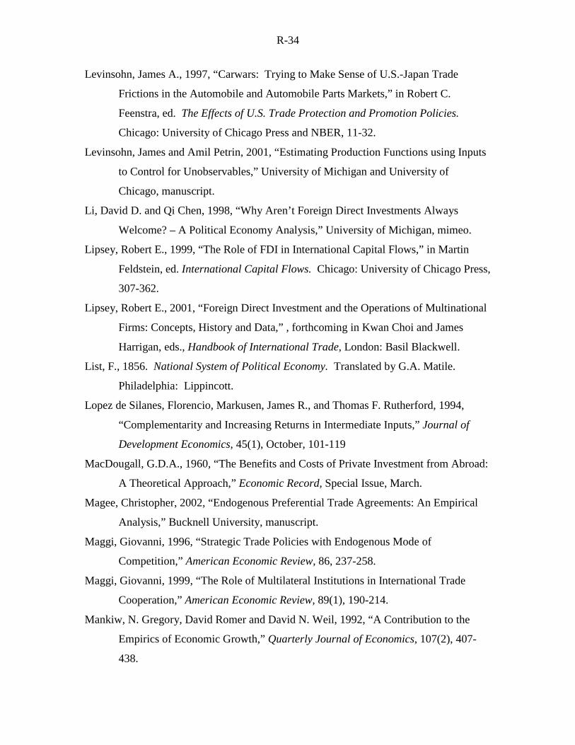
R-34
Levinsohn, James A., 1997, “Carwars: Trying to Make Sense of U.S.-Japan Trade
Frictions in the Automobile and Automobile Parts Markets,” in Robert C.
Feenstra, ed. The Effects of U.S. Trade Protection and Promotion Policies.
Chicago: University of Chicago Press and NBER, 11-32.
Levinsohn, James and Amil Petrin, 2001, “Estimating Production Functions using Inputs
to Control for Unobservables,” University of Michigan and University of
Chicago, manuscript.
Li, David D. and Qi Chen, 1998, “Why Aren’t Foreign Direct Investments Always
Welcome? – A Political Economy Analysis,” University of Michigan, mimeo.
Lipsey, Robert E., 1999, “The Role of FDI in International Capital Flows,” in Martin
Feldstein, ed. International Capital Flows. Chicago: University of Chicago Press,
307-362.
Lipsey, Robert E., 2001, “Foreign Direct Investment and the Operations of Multinational
Firms: Concepts, History and Data,” , forthcoming in Kwan Choi and James
Harrigan, eds., Handbook of International Trade, London: Basil Blackwell.
List, F., 1856. National System of Political Economy. Translated by G.A. Matile.
Philadelphia: Lippincott.
Lopez de Silanes, Florencio, Markusen, James R., and Thomas F. Rutherford, 1994,
“Complementarity and Increasing Returns in Intermediate Inputs,” Journal of
Development Economics, 45(1), October, 101-119
MacDougall, G.D.A., 1960, “The Benefits and Costs of Private Investment from Abroad:
A Theoretical Approach,” Economic Record, Special Issue, March.
Magee, Christopher, 2002, “Endogenous Preferential Trade Agreements: An Empirical
Analysis,” Bucknell University, manuscript.
Maggi, Giovanni, 1996, “Strategic Trade Policies with Endogenous Mode of
Competition,” American Economic Review, 86, 237-258.
Maggi, Giovanni, 1999, “The Role of Multilateral Institutions in International Trade
Cooperation,” American Economic Review, 89(1), 190-214.
Mankiw, N. Gregory, David Romer and David N. Weil, 1992, “A Contribution to the
Empirics of Economic Growth,” Quarterly Journal of Economics, 107(2), 407-
438.
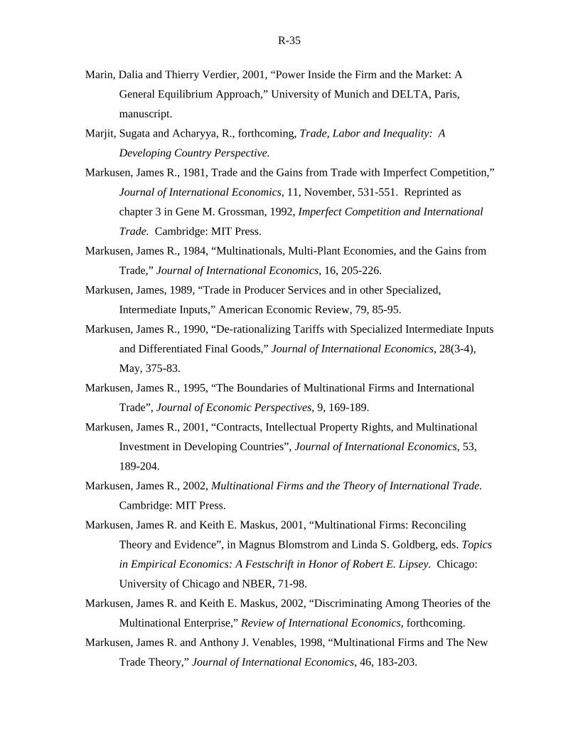
R-35
Marin, Dalia and Thierry Verdier, 2001, “Power Inside the Firm and the Market: A
General Equilibrium Approach,” University of Munich and DELTA, Paris,
manuscript.
Marjit, Sugata and Acharyya, R., forthcoming, Trade, Labor and Inequality: A
Developing Country Perspective.
Markusen, James R., 1981, Trade and the Gains from Trade with Imperfect Competition,”
Journal of International Economics, 11, November, 531-551. Reprinted as
chapter 3 in Gene M. Grossman, 1992, Imperfect Competition and International
Trade. Cambridge: MIT Press.
Markusen, James R., 1984, “Multinationals, Multi-Plant Economies, and the Gains from
Trade,” Journal of International Economics, 16, 205-226.
Markusen, James, 1989, “Trade in Producer Services and in other Specialized,
Intermediate Inputs,” American Economic Review, 79, 85-95.
Markusen, James R., 1990, “De-rationalizing Tariffs with Specialized Intermediate Inputs
and Differentiated Final Goods,” Journal of International Economics, 28(3-4),
May, 375-83.
Markusen, James R., 1995, “The Boundaries of Multinational Firms and International
Trade”, Journal of Economic Perspectives, 9, 169-189.
Markusen, James R., 2001, “Contracts, Intellectual Property Rights, and Multinational
Investment in Developing Countries”, Journal of International Economics, 53,
189-204.
Markusen, James R., 2002, Multinational Firms and the Theory of International Trade.
Cambridge: MIT Press.
Markusen, James R. and Keith E. Maskus, 2001, “Multinational Firms: Reconciling
Theory and Evidence”, in Magnus Blomstrom and Linda S. Goldberg, eds. Topics
in Empirical Economics: A Festschrift in Honor of Robert E. Lipsey. Chicago:
University of Chicago and NBER, 71-98.
Markusen, James R. and Keith E. Maskus, 2002, “Discriminating Among Theories of the
Multinational Enterprise,” Review of International Economics, forthcoming.
Markusen, James R. and Anthony J. Venables, 1998, “Multinational Firms and The New
Trade Theory,” Journal of International Economics, 46, 183-203.
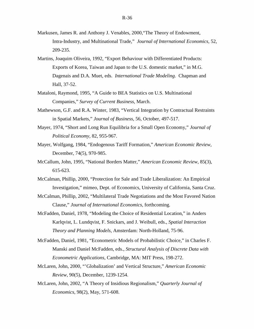
R-36
Markusen, James R. and Anthony J. Venables, 2000,“The Theory of Endowment,
Intra-Industry, and Multinational Trade,” Journal of International Economics, 52,
209-235.
Martins, Joaquim Oliveira, 1992, “Export Behaviour with Differentiated Products:
Exports of Korea, Taiwan and Japan to the U.S. domestic market,” in M.G.
Dagenais and D.A. Muet, eds. International Trade Modeling. Chapman and
Hall, 37-52.
Mataloni, Raymond, 1995, “A Guide to BEA Statistics on U.S. Multinational
Companies,” Survey of Current Business, March.
Mathewson, G.F. and R.A. Winter, 1983, “Vertical Integration by Contractual Restraints
in Spatial Markets,” Journal of Business, 56, October, 497-517.
Mayer, 1974, “Short and Long Run Equilibria for a Small Open Economy,” Journal of
Political Economy, 82, 955-967.
Mayer, Wolfgang, 1984, “Endogenous Tariff Formation,” American Economic Review,
December, 74(5), 970-985.
McCallum, John, 1995, “National Borders Matter,” American Economic Review, 85(3),
615-623.
McCalman, Phillip, 2000, “Protection for Sale and Trade Liberalization: An Empirical
Investigation,” mimeo, Dept. of Economics, University of California, Santa Cruz.
McCalman, Phillip, 2002, “Multilateral Trade Negotiations and the Most Favored Nation
Clause,” Journal of International Economics, forthcoming.
McFadden, Daniel, 1978, “Modeling the Choice of Residential Location,” in Anders
Karlqvist, L. Lundqvist, F. Snickars, and J. Weibull, eds., Spatial Interaction
Theory and Planning Models, Amsterdam: North-Holland, 75-96.
McFadden, Daniel, 1981, “Econometric Models of Probabilistic Choice,” in Charles F.
Manski and Daniel McFadden, eds., Structural Analysis of Discrete Data with
Econometric Applications, Cambridge, MA: MIT Press, 198-272.
McLaren, John, 2000, “’Globalization’ and Vertical Structure,” American Economic
Review, 90(5), December, 1239-1254.
McLaren, John, 2002, “A Theory of Insidious Regionalism,” Quarterly Journal of
Economics, 98(2), May, 571-608.
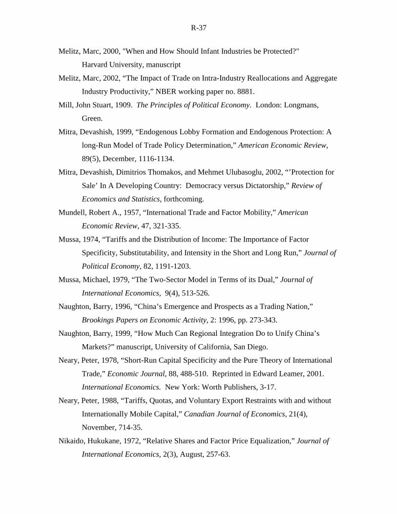
R-37
Melitz, Marc, 2000, "When and How Should Infant Industries be Protected?"
Harvard University, manuscript
Melitz, Marc, 2002, “The Impact of Trade on Intra-Industry Reallocations and Aggregate
Industry Productivity,” NBER working paper no. 8881.
Mill, John Stuart, 1909. The Principles of Political Economy. London: Longmans,
Green.
Mitra, Devashish, 1999, “Endogenous Lobby Formation and Endogenous Protection: A
long-Run Model of Trade Policy Determination,” American Economic Review,
89(5), December, 1116-1134.
Mitra, Devashish, Dimitrios Thomakos, and Mehmet Ulubasoglu, 2002, “’Protection for
Sale’ In A Developing Country: Democracy versus Dictatorship,” Review of
Economics and Statistics, forthcoming.
Mundell, Robert A., 1957, “International Trade and Factor Mobility,” American
Economic Review, 47, 321-335.
Mussa, 1974, “Tariffs and the Distribution of Income: The Importance of Factor
Specificity, Substitutability, and Intensity in the Short and Long Run,” Journal of
Political Economy, 82, 1191-1203.
Mussa, Michael, 1979, “The Two-Sector Model in Terms of its Dual,” Journal of
International Economics, 9(4), 513-526.
Naughton, Barry, 1996, “China’s Emergence and Prospects as a Trading Nation,”
Brookings Papers on Economic Activity, 2: 1996, pp. 273-343.
Naughton, Barry, 1999, “How Much Can Regional Integration Do to Unify China’s
Markets?” manuscript, University of California, San Diego.
Neary, Peter, 1978, “Short-Run Capital Specificity and the Pure Theory of International
Trade,” Economic Journal, 88, 488-510. Reprinted in Edward Leamer, 2001.
International Economics. New York: Worth Publishers, 3-17.
Neary, Peter, 1988, “Tariffs, Quotas, and Voluntary Export Restraints with and without
Internationally Mobile Capital,” Canadian Journal of Economics, 21(4),
November, 714-35.
Nikaido, Hukukane, 1972, “Relative Shares and Factor Price Equalization,” Journal of
International Economics, 2(3), August, 257-63.
R-38
Obstfeld, Maurice and Kenneth Rogoff, 2000, “The Six Major Puzzles in International
Macroeconomics: Is There a Common Cause?” in Ben S. Bernanke and Kenneth
Rogoff, eds., NBER Macroeconomics Annual, 2000. Cambridge: MIT Press,
339-389.
Ohyama, M., 1972, “Trade and Welfare in General Equilibrium,” Keio Economic Studies,
9, 37-73.
Olley, G. Steven and Ariel Pakes, 1996, “The Dynamics of Productivity in the
Telecommunications Equipment Industry,” Econometrica, 64(6), November,
1263-1297.
Ordover, Janusz A., Garth Saloner and Steven C. Salop, 1990, “Equilibrium Vertical
Foreclosure,” American Economic Review, 80(1), March, 127-142.
Ordover, Janusz A., Garth Saloner and Steven C. Salop, 1992, “Equilibrium Vertical
Foreclosure: Reply,” American Economic Review, 82(3), June, 698-703.
Overman, Henry, Stephen Redding and Anthony J. Venables, 2003, “Trade and
Geography: A Survey of Empirics,” in Kwan Choi and James Harrigan, eds.,
Handbook of International Trade, Basil Blackwell, forthcoming.
Panagariya, Arvind, 2000, “Evaluating the Factor-Content Approach to Measuring the
Effect of Trade on Wage Inequality?”, Journal of International Economics, 50,
91-116.
Pavcnik, Nina, 2002, “Trade Disputes in the Commercial Aircraft Industry,” World
Economy, 25, 733-751.
Perry, Martin K., 1989, “Vertical Integration: Determinants and Effects,” in Richard
Schmalansee and Robert Willig, eds. Handbook of Industrial Organization,
volume 1. North-Holland: Amsterdam, 185-255.
Perry, Martin K. and Robert H. Porter, 1985, “Oligopoly and the Incentive for Horizontal
Merger,” American Economic Review, 75(1), 219-227.�
Phelps, Edmund S., 1997, Rewarding Work. Cambridge: Harvard University Press.
Pollak, R.A., 1989, The Theory of the Cost-of-Living Index, Oxford: Oxford University
Press.
Prebisch, Raul, 1950, The Economic Development of Latin America and Its Principal
Problems. New York: United Nations.
R-39
Prusa, Thomas J., 1991, “The Selection of Anti-Dumping Cases for Withdrawal,” in
Robert E. Baldwin, ed. Empirical Studies of Commercial Policy. Chicago: Univ.
of Chicago and NBER.
Prusa, Thomas J., 1992, “Why Are So Many Antidumping Petitions Withdrawn?”
Journal of International Economics, 33, 1-20.
Prusa, Thomas J., 2001, “On the Spread and Impact of Anti-Dumping.” Canadian
Journal of Economics, 34(3), August, 591-611.
Puga, Diego and Daniel Trefler, 2002, “Knowledge Creation and Control in
Organizations,” University of Toronto, manuscript.
Rauch, James E., 1999, “Networks versus Markets in International Trade,” Journal of
International Economics, 48(1), June, 7-37.
Rauch, James E., 2001, “Business and Social Networks in International Trade,” Journal
of Economic Literature, 39, December, 1177-1203.
Rauch, James E. and Alessandra Casella, 2001, Networks and Markets. New York:
Russell Sage.
Rauch, James E. and Alessandra Casella, 2003, “Overcoming Informational Barriers to
International Resource Allocation: Prices and Group Ties,” Economic Journal,
forthcoming.
Rauch, James E. and Vitor Trindade, 2000, “Information and Globalization: Wage Co-
Movements, Labor Demand Elasticity, and Conventional Trade Liberalization”
NBER Working Paper no. 7671.
Rauch, James E. and Vitor Trindade, 2002, “Ethnic Chinese Networks in International
Trade,” Review of Economics and Statistics, 84(1), February, 116-130.
Rauch, James E. and Joel Watson, 2002, “Entrepreneurship and International Trade,”
NBER Working Paper no. 8708.
Redding, Stephen and Anthony J. Venables, 2000, “Economic Geography and
International Inequality,” Center for Economic Policy Research, Discussion paper
no. 2568.
Redding, Stephen, 2002, “Specialization Dynamics,” Journal of International
Economics, forthcoming.
R-40
Reid, Peter C., 1990. Made Well in America: Lessons from Harley-Davidson on Being
the Best. New York: McGraw-Hill.
Ricardo, David, 1951, The Works and Correspondence of David Ricardo, P. Sfaffa, ed.
Cambridge: Cambridge University Press.
Richardson, J. David, 1982, “Trade Adjustment Assistance under the Trade Act of 1974:
An Analytical Examination and Worker Survey,” in Jagdish N. Bhagwati, ed.
Import Competition and Response. Chicago: Univ. of Chicago and NBER, 321-
357.
Richardson, J. David, 1995, “Income Inequality and Trade: How to Think, What to
Conclude”, Journal of Economic Perspectives, 9(3), Summer, 33-56.
Ries, John, 1993, “Windfall Profits and Vertical Relationships: Who Gained in the
Japanese Auto Industry from VERs?” Journal of Industrial Economics, 41(3),
259-276.
Rivera-Batiz, Luis A. and Paul Romer, 1991a, “Economic Integration and Economic
Growth,” Quarterly Journal of Economics, 106, 531-555.
Rivera-Batiz, Luis A. and Paul Romer, 1991b, “International Trade with Endogenous
Technological Change,” European Economic Review, 35, 971-1004.
Robertson, Raymond, 2000, “Relative Prices and Wage Inequality: Evidence from
Mexico,” mimeo, Macalester College.
Robinson, Joan, 1933, The Economics of Imperfect Competition. London, Macmillan.
Rodriguez, Carlos A., 1979, “The Quality of Imports and the Differential Effects of
Tariffs, Quotas, and Quality Controls as Protective Devices,” Canadian Journal
of Economics, 12(3), August, 439-449.
Rodriguez, Francisco and Dani Rodrik, 2000, “Trade Policy and Economic Growth: A
Skptic’s Guide to the Cross-Nationa lEvidence,” in Ben S. Gernanke and Kenneth
Rogoff, eds., NBER Macroeconomics Annual 2000, 261-325.
Rodrik, D., 1997, Has Globalization Gone Too Far? Institute for International
Economics: Washington, D.C.
Rodrik, Dani, 1993, “Industrial Organization and Product Quality: Evidence from South
Korean and Taiwanese Exports,” in Paul Krugman and Alasdair Smith, eds.,
R-41
Empirical Studies of Strategic Trade Policy. Chicago: Univ. of Chicago and
NBER, 195-210.
Rodrik, Dani, 1995, “Taking Trade Policy Seriously: Export Subsidization as a Case
Study in Policy Effectiveness,” in Jim Levinsohn, Alan V. Deardorff, and Robert
M. Stern, New Directions in Trade Theory. Michigan: University of Michigan
Press, 347-384.
Rodrik, Dani, 1995, “The Political Economy of Trade Policy,” in Gene M. Grossman and
Kenneth Rogoff, eds., Handbook if International Economics, vol. III.
Amsterdam: Elsevier, pp. 1457-1494.
Romalis, John, 2001, “Factor Proportions and the Structure of Commodity Trade,”
University of Chicago, manuscript.
Romalis, John, 2002, “NAFTA’s and CUSFTA’s Impact on North American Trade,”
University of Chicago, manuscript.
Romer, Paul, 1990, “Endogenous Technical Change,” Journal of Political Economy,
98(5, Part 2), S71-S102.
Romer, Paul, 1994, “New Goods, Old Theory, and the Welfare Costs of Trade
Restrictions,” Journal of Development Economics, 43, 5-38.
Rose, Andrew K. and Eric van Wincoop, 2001, “National Monday as a Barrier to
International Trade: The Real Case for Currency Union,” American Economic
Review, 91(2), May, 386-390.
Rosen, Daniel, 1998, Behind the Open Door: Foreign Firms in China, Institute for
International Economics, Washington, D.C.
Rosen, Sherwin, 1974, “Hedonic Prices and Implicit Markets: Product Differentiation in
Pure Competition,” Journal of Political Economy, 34-55.
Rybczynski, T.N., 1955, “Factor Endowments and Relative Commodity Prices,”
Economica, 22, 336-341.
Sachs, Jeffrey D., 2001. “Tropical Underdevelopment,” NBER Working Paper no. 8119.
Sachs, Jeffrey D. and Howard J. Shatz, 1994, “Trade and Jobs in U.S. Manufacturing,”
Brookings Papers on Economic Activity, 1, 1-84.
R-42
Sachs, Jeffrey D. and Howard J. Shatz, 1998, “International Trade and Wage Inequality:
Some New Results,” in Susan M. Collins, ed., Imports, Exports, and the
American Worker, Washington, DC: Brookings Institution Press, 215-240.
Sachs, Jeffrey and Andrew Warner, 1995, “Economic Reform and the Precess of Global
Integration,” Brooking Papers on Economic Activity, 1, 1-118.
Samuelson, Paul A., 1949, “International Factor Price Equalization Once Again,”
Economic Journal, June, 181-197. Reprinted in Edward E. Leamer, ed. 2001,
International Economics, New York: Worth Publishers, 19-32.
Samuelson, Paul A, 1952, “The Transfer Problem and Transport Costs: The Terms of
Trade when Impediments are Absent,” Economic Journal, 62, 278-304.
Samuelson, Paul A., 1953-54, “The Prices of Goods and Factor in General Equilibrium,”
Review of Economic Studies, 21(1), 1-20
Samuelson, Paul A., 1956, “Social Indifference Curves,” Quarterly Journal of
Economics, 70,(1) February, 1-22.
Samuelson, Paul A., 1962, “The Gains from International Trade Once Again,” Economic
Journal, 72, 820-829.
Samuelson, Paul A., 2001, “The Ricardo-Sraffa Paradigm Comparing Gains from Trade
in Inputs and Finished Products,” Journal of Economic Literature, 39, December,
1204-1214.
Schiff, Maurice and Won Chang, 2002, “Market Presence, Contestability, and the Terms
of Trade Effects of Regional Integration,” Journal of International Economics,
forthcoming.
Schott, Peter, 2000, “One Size Fits All? Heckscher-Ohlin Specialization in Global
Production,” Yale University, manuscript.
Segerstrom, Paul, Anant, T.C.A. and Elias Dinopoulos, 1990, “A Schumpeterian Model
of the Product Life Cycle,” American Economic Review, 80, 1077-1099.
Shiells, Clinton R., Robert M. Stern and Alan V. Deardorff, 1986, “Estimates of the
Elasticities of Substitution between Imports and Home Goods for the United
States,” Weltwirtschaftliches Archiv, 122(3), 497-519.
Slater, Joanna and Eriko Amaha, 1999, “Masters of the Trade,” Far Eastern Economic
Review, July 22: 10-14.
R-43
Slaughter, Matthew J., 2000, “What Are the Results of Product-Price Studies and What
Can We Learn from Their Differences?” in Robert C. Feenstra, ed., The Effects of
International Trade on Wages, Chicago: University of Chicago Press, 129-165.
Slaughter, Matthew J., 2001, “International Trade and Labor-Demand Elasticities,”
Journal of International Economics, 54, 27-56.
Smith, M. Alasdair, 1977, “Capital Accumulation in the Open Two-Sector Economy,”
Economic Journal, 87(346), June, 273-282.
Solow, Robert M., 1956, “A Contribution to the Theory of Economic Growth,” Quarterly
Journal of Economics, 70, 65-94.
Solow, Robert M., 1957, “Technical Change and the Aggregate Production Function,”
Review of Economics and Statistics, 39, 312-320.
Spence, A. Michael, 1975, “Monopoly, Quality, and Regulation,” The Bell Journal of
Economics, 6(2), Autumn, 417-429.
Spence, Michael, “Product Selection, Fixed Costs, and Monopolistic Competition,”
Review of Economic Studies, 43(2), June 1976, 217-235.
Staiger, Robert, 1986, “Measurement of the Factor Content of Foreign Trade with Traded
Intermediate Goods,” Journal of International Economics, 21, 361-368.
Staiger, Robert W. and Frank A. Wolak, 1992, “The Effect of Antidumping Law in the
Presence of Foreign Monopoly,” Journal of International Economics, 32, May,
265-287.
Staiger, Robert W. and Frank A. Wolak, 1994, “Measuring Industry-Specific Protection:
Antidumping in the United States,” Brooking Papers on Economic Activity:
Microeconomics, 51-118.
Stolper, Wolfgang F. and Paul A. Samuelson, 1941, “Protection and Real Wages,”
Review of Economic Studies, 9, 58-73.
Solow, Robert M., 1956, “A Contribution to the Theory of Economic Growth,” Quarterly
Journal of Economics, 60(1), 65-94.
Solow, Robert M., 1957, “Technical Change and the Aggregate Production Function,”
The Review of Economics and Statistics, 39(3), August, 312-320.
Suomela, John W., 1993. Free Trade versus Fair Trade: The Making of American Trade
Policy in a Political Environment. Turku, Finland: Institute for European Studies.
R-44
Swan, Peter L., 1970, “Durability of Consumption Goods,” American Economic Review,
60(5), December, 884-894.
Swenson, Deborah, 2002, “Foreign Investment and the Mediation of Trade Flows,”
Review of International Economics, forthcoming.
Taylor, M. Scott, 1993, “’Quality Ladders’ and Ricardian Trade,” Journal of
International Economics, 34, 225-243.
Taylor, M. Scott, 1994, “’Once-off’ and Continuing Gains from Trade,” Review of
Economic Studies, 61, 589-601.
Tinbergen, Jan, 1962, Shaping the World Economy. New York: The Twentieth Century
Fund.
Tombazos, Christis G., 1999, “The Role of Imports in Expanding the Demand Gap
Between Skilled and Unskilled Labor in the U.S.,” Applied Economics, 31, 509-
516.
Törnqvist, L., 1936, “The Bank of Finland’s Consumption Price Index,” Bank of Finland
Monthly Bulletin 10: 1-8.
Train, Kenneth, 1986, Qualitative Choice Analysis. Cambridge: MIT Press.
Trefler, Daniel, 1993, “International Factor Price Differences: Leontief was Right!”
Journal of Political Economy, December, 961-987.
Trefler, Daniel, 1993, “International Factor Price Differences: Leontief was Right!”
Journal of Political Economy, December, 961-987.
Trefler, Daniel, 1993, “Trade Liberalization and the Theory of Endogenous Protection,”
Journal of Political Economy, February, 101(1), 138-160.
Trefler, Daniel, 1995, “The Case of Missing Trade and Other Mysteries,” American
Economic Review, December, 85(5), 1029-1046. Reprinted in Edward E. Leamer,
ed. 2001, International Economics, New York: Worth Publishers, 151-175.
Trefler, Daniel, 1998, “The Structure of Factor Content Predictions,” University of
Toronto, manuscript.
Trefler, Daniel, 2001, “The Long and Short of the Canada-U.S. Free Trade Agreement,”
NBER Working Paper No. 8293.
Trefler, Daniel and Susan Chun Zhu, 2000 “Beyond the Algebra of Explanation: HOV
for the Technology Age,” American Economic Review, May 2000, 145-149.
R-45
Turunen-Red, Arja H. and Alan D. Woodland, 1991, “Strict Pareto Improving Reforms
of Tariffs,” Econometrica, 59, 1127-1152.
Turunen-Red, Arja H. and Alan D. Woodland, 2000, “Multilateral Policy Reforms and
Quantity Restrictions on Trade,” Journal of International Economics, 52(1),
October, 153-168.
Tybout, James R., Jamie de Melo, and Vittorio Corbo, 1991, “The effects of Trade
Reform on Scale and Technical Efficiency,” New Evidence from Chile,” Journal
of International Economics, 31(3/4), 231-250.
Tybout, James R. and M. Daniel Westbrook, 1995, “Trade Liberalization and Dimensions
of Efficiency Change in Mexican Manufacturing Industries,” Journal of
International Economics, 39(1/2), 53-78.
Tyson, Laura D’Andrea, 1992, Who’s Bashing Whom: Trade Conflict in High
Technology Industries. Washington, D.C.: Institute for International Economics.
United Nations, 1996, World Investment Report. New York.
United States Department of Commerce, Bureau of Economic Analysis, 1995, Foreign
Direct Investment in the United States, 1992 Benchmark Survey, Final Results.
Washington, D.C.
United States International Trade Commission, 1983, Heavyweight Motorcycles, and
Engines and Power Train Subassemblies Therefor. Publication 1342,
Washington, D.C.
United States International Trade Commission, 1983-84, Heavyweight Motorcycles:
Quarterly Report on Selected Economic Indicators. Various publications,
Washington, D.C.
van Ark, Bart, Erik Monnikhof and Marcel Timmer, 1999, “Prices, Quantities, and
Productivity in Industry: A Study of Transition Economies in a Comparative
Perspective,” in Alan Heston and Robert E. Lipsey, International and Interarea
Comparisons of Income, Output, and Prices, NBER Studies in Income and
Wealth, no. 61, Chicago: Univ. of Chicago, 327-364.
Vanek, Jaroslav, 1968, “The Factor Proportions Theory: The N-Factor Case,” Kyklos, 21,
October, 749-754.
R-46
Vartia, Y.O., 1976a, Relative Changes and Index Numbers, Helsinki: The Research
Institute of the Finnish Economy.
Vartia, Y.O., 1976b, “Ideal Log-Change Index Numbers”, Scandinavian Journal of
Statistics 3, 121-126.
Ventura, Jaume, 1997, “Growth and Interdependence,” Quarterly Journal of Economics,
107(1), February, 57-84.
Viner, J., 1950, The Customs Union Issue. New York: Carnegie Endowment for
International Peace.
Viner, Jacob, 1966. Dumping: A Problem in International Trade. New York: Augustus
M. Kelley, Publishers.
Wei, Shang-Jin, 1998, “Why Does China Attract so Little Foreign Investment?” Harvard
University and NBER, mimeo.
Weinstein, David E., 1992, “Competition and Unilateral Dumping,” Journal of
International Economics, 32, 379-388.
Williamson, Oliver E. 1975. Markets and Hierarchies: Analysis and Antitrust
Implications. New York: Free Press.
Williamson, Oliver E. ,1985, The Economic Institutions of Capitalism. New York: The
Free Press.
Wong, Kar-yiu, 1989, “Optimal Threat of Trade Restriction and Quid Pro Quo Foreign
Investment,” Economics and Politics, 1, 277-300.
Wood, Adrian, 1995, “How Trade Hurt Unskilled Workers,” Journal of Economic
Perspectives, 9(3), Summer, 57-80.
Woodland, Alan D., 1977, “A Dual Approach to Equilibrium in the Production Sector in
International Trade Theory,” Canadian Journal of Economics, 10, 50-68.
Woodland, Alan D., 1982, International Trade and Resource Allocation, Amsterdam:
North-Holland.
World Bank, 1993, The East Asian Miracle: Economic Growth and Public Policy.
Oxford: Oxford University Press.
Xu, Bin, 2002, “Capital Abundance and Developing Country Production Patterns,”
University of Florida, manuscript.
R-47
Yeaple, Dennis, 2002, “A Simple Model of Firm Heterogeneity, International Trade, and
Wages,” University of Pennsylvania, manuscript.
Yeung, Henry Wai-chung, 2001, “Organizing Regional Production Networks in
Southeast Asia: Implications for Production Fragmentation, Trade and Rules of
Origin,” Journal of Economic Geography, 1(3), 299-321.
Yi, Kei-Mu, 2001, “Can Vertical Specialization Explain the Growth of World Trade?,”
Journal of Political Economy, forthcoming.
Young, Alwyn, 1997, “The Razor’s Edge: Distortions and Incremental Reform in the
People’s Republic of China, University of Chicago, mimeo.
Zhu, Susan Chun, 2001a, “Trade, Product Cycles and Inequality Within and Between
Countries,” Michigan State University, manuscript.
Zhu, Susan Chun, 2001b, “Trade, Product Cycles and Wage Inequality: An International
Perspective,” Michigan State University, manuscript.
Zhu, Susan Chun and Daniel Trefler, 2001, “Ginis in General Equilibrium: Trade,
Technology and Southern Inequality,” NBER working paper no. 8446.