Embed Size (px)
Citation preview
Advanced Macroeconomics I/AYouzhi Yang
Department of EconomicsShanghai University of Finance and Economics
Fall 2013
Advanced Macroeconomics I/A 2
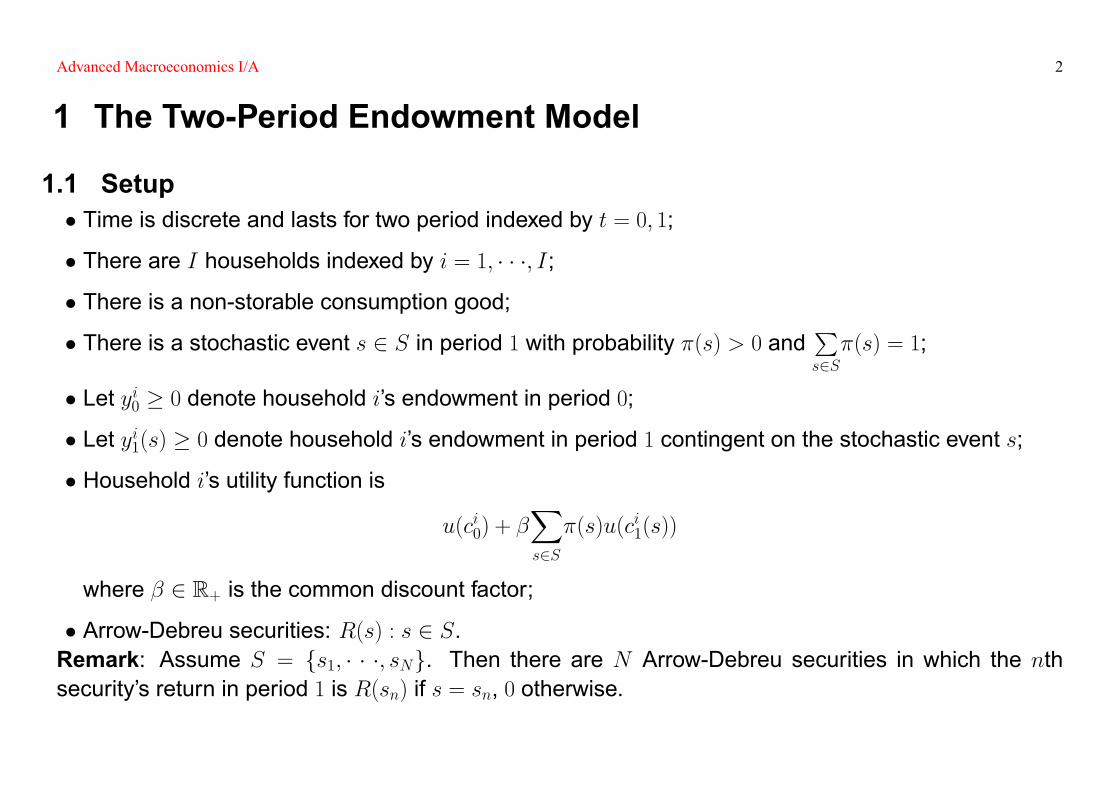
1 The Two-Period Endowment Model
1.1 Setup� Time is discrete and lasts for two period indexed by t = 0; 1;
� There are I households indexed by i = 1; � � �; I;
� There is a non-storable consumption good;
� There is a stochastic event s 2 S in period 1 with probability �(s) > 0 andPs2S�(s) = 1;
� Let yi0 � 0 denote household i's endowment in period 0;
� Let yi1(s) � 0 denote household i's endowment in period 1 contingent on the stochastic event s;
� Household i's utility function is
u(ci0) + �Xs2S�(s)u(ci1(s))
where � 2 R+ is the common discount factor;
� Arrow-Debreu securities: R(s) : s 2 S.Remark: Assume S = fs1; � � �; sNg. Then there are N Arrow-Debreu securities in which the nthsecurity's return in period 1 is R(sn) if s = sn, 0 otherwise.
Advanced Macroeconomics I/A 3
1.2 The Budget Constraints
ci0 +Xs2Ski(s) � yi0
ci1(s) � yi1(s) +R(s)ki(s) for all s 2 S
+
ci0 +Xs2S
ci1(s)
R(s)� yi0 +
Xs2S
yi1(s)
R(s)| {z }Lifetime Income
� Y i (1)
1.3 Household i's Optimization ProblemGiven R(s) : s 2 S, household i's optimization problem is
maxci0;c
i1(s):s2S
(u(ci0) + �
Xs2S�(s)u(ci1(s))
)
Advanced Macroeconomics I/A 4
subject to
ci0 +Xs2S
ci1(s)
R(s)� yi0 +
Xs2S
yi1(s)
R(s)� Y i
ci0 � 0
ci1(s) � 0 for all s 2 S
Let � be the Lagrangian multiplier for the intertemporal budget constraint. Then, the Kuhn-Tucherconditions are as follows:
u0(ci0)� � � 0, ci0 � 0, and (u0(ci0)� �)ci0 = 0
��(s)u0(ci1(s))� �=R(s) � 0, ci1(s) � 0, and (��(s)u0(ci1(s))� �=R(s))ci1(s) = 0
Y i � ci0 +
Xs2S
ci1(s)
R(s)
!� 0, � � 0, and
"Y i �
ci0 +
Xs2S
ci1(s)
R(s)
!#� = 0
De�nition 1 The utility function satis�es the Inada conditions if
u0 > 0, u00 < 0, limc!0u0(c) =1, and lim
c!1u0(c) = 0.
Advanced Macroeconomics I/A 5
If the utility function satis�es the Inada conditions, then
u0(ci0) = ��(s)R(s)u0(ci1(s)) for all s 2 S (2)
which is called the Euler's equation.Question: Try to prove the statement above.
1.4 The Market Clearing ConditionsAn Equilibrium consists of an allocation fci0; ci1(s); ki(s) : s 2 SgIi=1 and a price system fR(s) : s 2 Sgsuch that(i) Given the price system, household i maximizes its expected utility with fci0; ci1(s); ki(s) : s 2 Sg suchthat
u0(ci0) = ��(s)R(s)u0(ci1(s)) for all s 2 S
ci0 +Xs2Ski(s) = yi0
ci1(s) = yi1(s) +R(s)k
i(s) for all s 2 S
Advanced Macroeconomics I/A 6
(ii) For the security markets,IXi=1
ki(s) = 0 for all s 2 S;
(iii) For the good markets,IXi=1
yi0 =
IXi=1
ci0
IXi=1
yi1(s) =
IXi=1
ci1(s) for all s 2 S.
1.5 Linear Quadratic Permanent Income TheoryAssume the quadratic utility function u(c) = �(c � )2, and there only exists a risk-free asset with�R
F= 1. Then,
ci0 =Xs2S�(s)ci1(s)| {z }
Random Walk
=) ci0 =1 + r
2 + rE0�yi0 +
yi1(s)
1 + r
�| {z }
Permanent Income
where r � RF � 1
Advanced Macroeconomics I/A 7
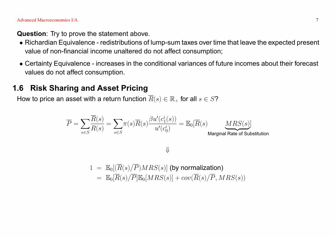
Question: Try to prove the statement above.� Richardian Equivalence - redistributions of lump-sum taxes over time that leave the expected presentvalue of non-�nancial income unaltered do not affect consumption;
� Certainty Equivalence - increases in the conditional variances of future incomes about their forecastvalues do not affect consumption.
1.6 Risk Sharing and Asset PricingHow to price an asset with a return function R(s) 2 R+ for all s 2 S?
P =Xs2S
R(s)
R(s)=Xs2S�(s)R(s)
�u0(ci1(s))
u0(ci0)= E0[R(s) MRS(s)| {z }]
Marginal Rate of Substitution
+
1 = E0[(R(s)=P )MRS(s)] (by normalization)= E0[R(s)=P ]E0[MRS(s)] + cov(R(s)=P ;MRS(s))
Advanced Macroeconomics I/A 8
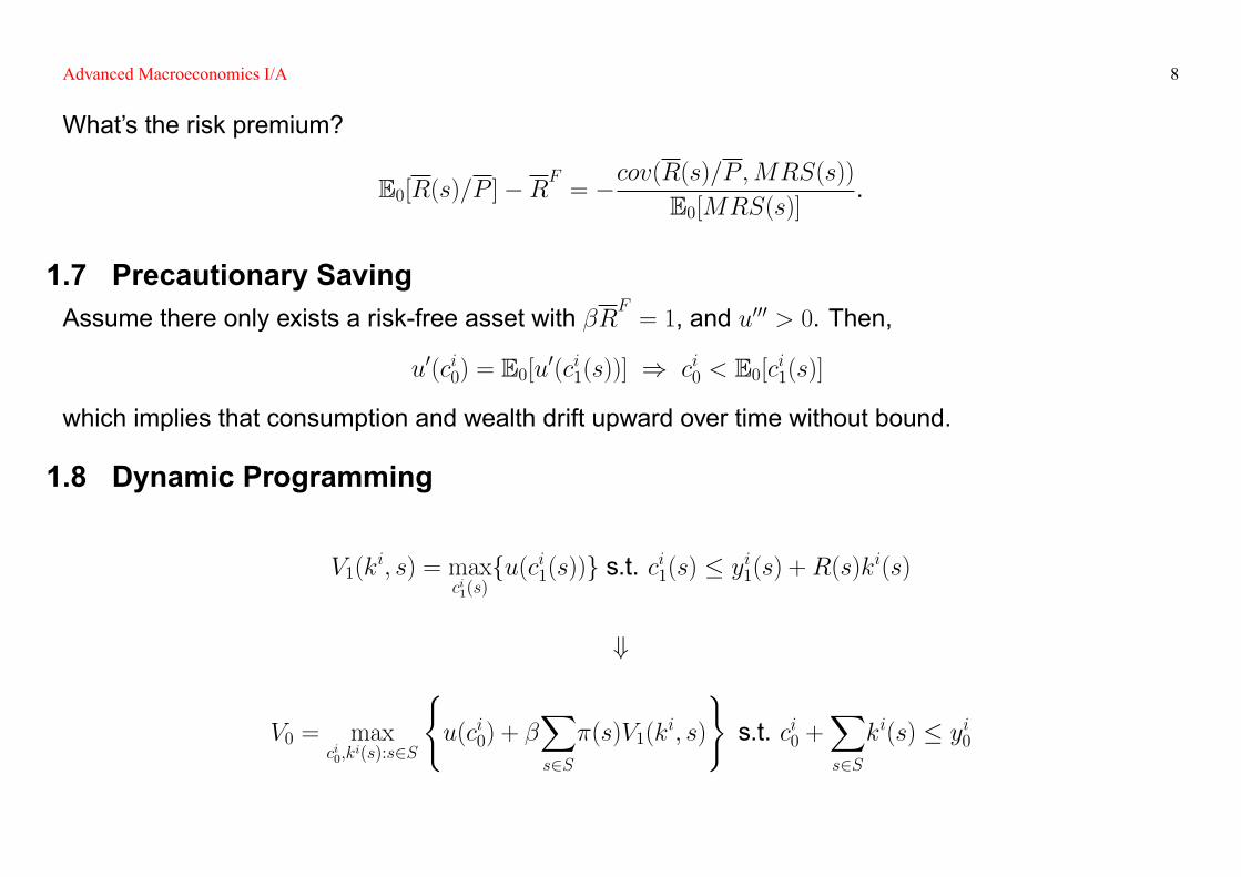
What's the risk premium?
E0[R(s)=P ]�RF= �cov(R(s)=P ;MRS(s))
E0[MRS(s)].
1.7 Precautionary SavingAssume there only exists a risk-free asset with �RF = 1, and u000 > 0. Then,
u0(ci0) = E0[u0(ci1(s))] ) ci0 < E0[ci1(s)]
which implies that consumption and wealth drift upward over time without bound.
1.8 Dynamic Programming
V1(ki; s) = max
ci1(s)fu(ci1(s))g s.t. ci1(s) � yi1(s) +R(s)ki(s)
+
V0 = maxci0;k
i(s):s2S
(u(ci0) + �
Xs2S�(s)V1(k
i; s)
)s.t. ci0 +
Xs2Ski(s) � yi0
Advanced Macroeconomics I/A 9
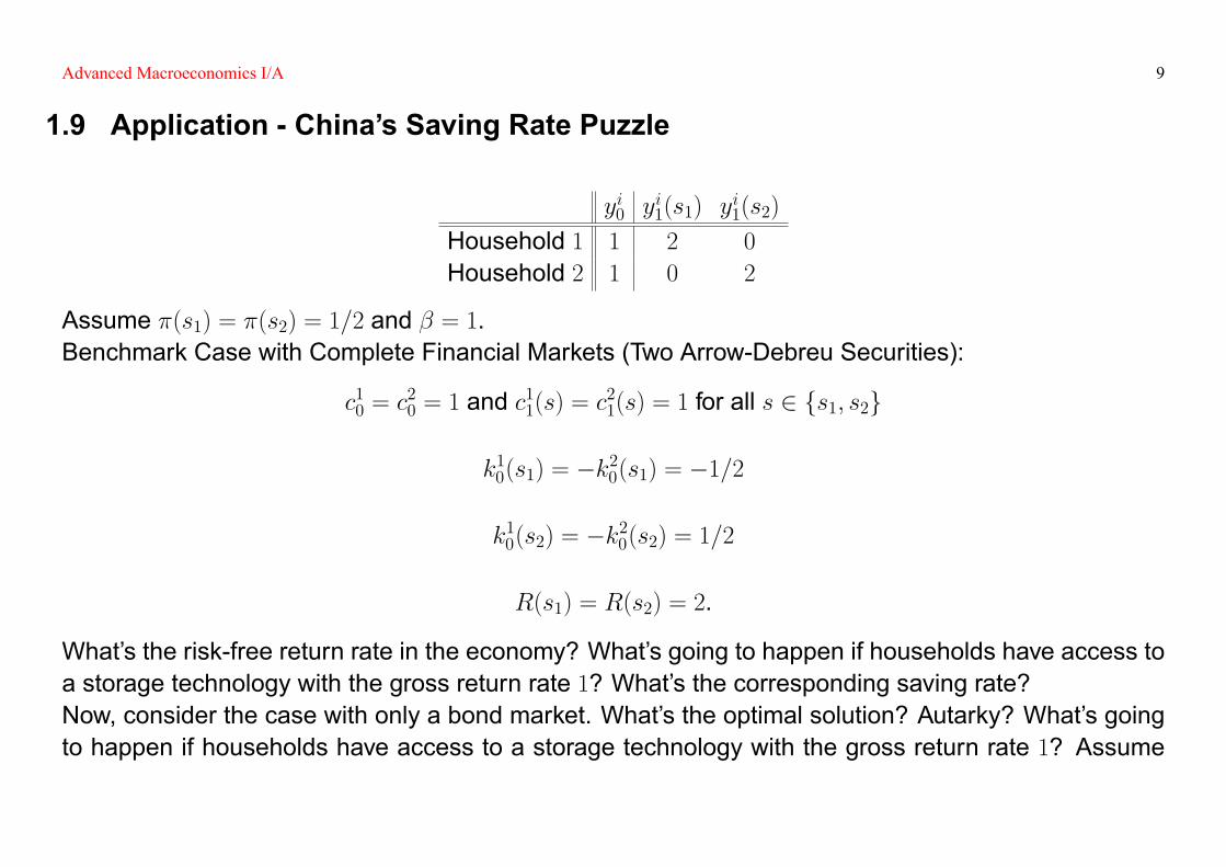
1.9 Application - China's Saving Rate Puzzle
yi0 yi1(s1) y
i1(s2)
Household 1 1 2 0
Household 2 1 0 2
Assume �(s1) = �(s2) = 1=2 and � = 1.Benchmark Case with Complete Financial Markets (Two Arrow-Debreu Securities):
c10 = c20 = 1 and c
11(s) = c
21(s) = 1 for all s 2 fs1; s2g
k10(s1) = �k20(s1) = �1=2
k10(s2) = �k20(s2) = 1=2
R(s1) = R(s2) = 2.
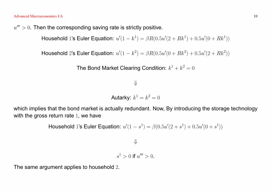
What's the risk-free return rate in the economy? What's going to happen if households have access toa storage technology with the gross return rate 1? What's the corresponding saving rate?Now, consider the case with only a bond market. What's the optimal solution? Autarky? What's goingto happen if households have access to a storage technology with the gross return rate 1? Assume
Advanced Macroeconomics I/A 10
u000 > 0. Then the corresponding saving rate is strictly positive.
Household 1's Euler Equation: u0(1� k1) = �R(0:5u0(2 +Rk1) + 0:5u0(0 +Rk1))
Household 2's Euler Equation: u0(1� k2) = �R(0:5u0(0 +Rk2) + 0:5u0(2 +Rk2))
The Bond Market Clearing Condition: k1 + k2 = 0
+
Autarky: k1 = k2 = 0
which implies that the bond market is actually redundant. Now, By introducing the storage technologywith the gross return rate 1, we have
Household 1's Euler Equation: u0(1� s1) = �(0:5u0(2 + s1) + 0:5u0(0 + s1))
+
s1 > 0 if u000 > 0.
The same argument applies to household 2.
Advanced Macroeconomics I/A 11
Conclusion: the under-development of �nancial markets could increase the saving rate, which pro-vides a potential explanation for the high saving rate in China.Question: what happens to the saving rate in both cases given
yi0 yi1(s1) y
i1(s2)
Household 1 1 3 �1Household 2 1 �1 3
which implies higher idiosyncratic risks.
1.10 References & Further Readings[1] Recursive Macroeconomic Theory, Chapter 1.
Advanced Macroeconomics I/A 12
2 The Solow Growth Model
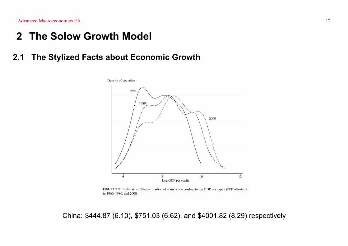
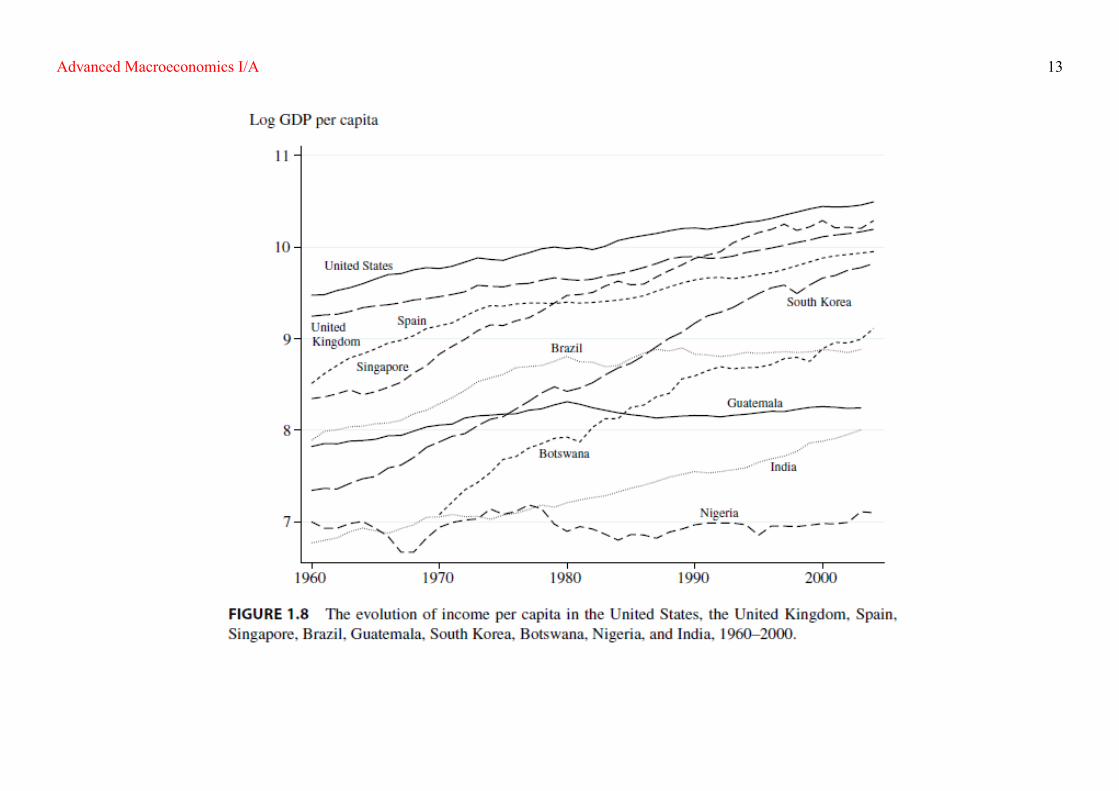
2.1 The Stylized Facts about Economic Growth
China: $444.87 (6.10), $751.03 (6.62), and $4001.82 (8.29) respectively
Advanced Macroeconomics I/A 13
Advanced Macroeconomics I/A 14
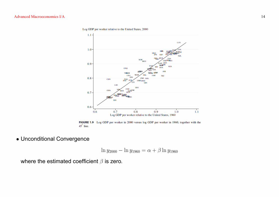
� Unconditional Convergence
ln y2000 � ln y1960 = � + � ln y1960
where the estimated coef�cient � is zero.
Advanced Macroeconomics I/A 15
� Conditional Convergence
ln y2000 � ln y1960 = � + � ln y1960 + X1960
where X1960 is a set of country-speci�c controls, such as levels of education, �scal and monetarypolicies, market competition, etc. Then, the estimated coef�cient � turns out to be around 2% perannum.
2.1.1 The Stylized Facts by Kaldor (1963)� Per capita output grows over time, and its growth rate does not tend to diminish.
� Physical capital per worker grows over time.
� The rate of return to capital is nearly constant.
� The ratio of physical capital to output is nearly constant.
� The shares of labor and physical capital in national income are nearly constant.
� The growth rate of output per worker differs substantially across countries.
2.1.2 Proximate vs. Fundamental Causes� Proximate causes: physical capital, human capital, and technology.
� Fundamental causes: institutional differences, cultural differences, and geographic differences.
Advanced Macroeconomics I/A 16
2.2 Setup� Time is discrete and lasts forever indexed by t = 0; 1; � � �;
� There is a continuum of households indexed by i 2 [0; 1];
� The number of heads in each household grows at a constant rate n � 0 such that Lit = (1 + n)tLi0;
� There is a competitive supply of entrepreneurs;
� There is a consumption/investment good;
� Household i holds a �xed fraction �i of the aggregate index of stocks in the economy withR�idi = 1;
� Each entrepreneur has access to the same "neoclassical" production technology as follows:
Y = F (K;L;A)
where
Technology A is a free public good;
Both capital and labor are necessary: F (0; L; A) = F (K; 0; A) = 0;
Constant returns to scale: F (mK;mL;A) = mF (K;L;A) for all m � 0;
Advanced Macroeconomics I/A 17
Inada conditions: Fx > 0, Fxx < 0, limx!0Fx =1, and lim
x!1Fx = 0 for x 2 fK;Lg.
2.3 Analysis
2.3.1 Household i's ProblemHousehold i's budget constraint in period t is
rtKit + wtL
it + �
it = Y
it = C
it + I
it
+
rtkit + wt + �
it = y
it = c
it + i
it (3)
where yit � Y it =Lit; k
it � K i
t=Lit; �
it � �it=L
it; c
it � C it=L
it; i
it � I it=L
it are the income, capital, dividend,
consumption, and investment per head of household i in period t, and rt and wt are the capital rentalprice and wage in period t. Given � 2 [0; 1] as the capital depreciation rate, we have
K it+1 = (1� �)K i
t + Iit
+
Advanced Macroeconomics I/A 18
(1 + n)kit+1 = (1� �)kit + iit. (4)
Furthermore, assume a �xed fraction s 2 [0; 1] of income is saved such that
cit = (1� s)yit and iit = syit. (5)
2.3.2 Entrepreneur j's Pro�t Maximization ProblemEntrepreneur j tries to maximize pro�t as follows:
maxKjt ;L
jt
fF (Kjt ; L
jt ; At)� rtK
jt � wtL
jtg
+
FOCs: FK(Kjt ; L
jt ; At) = rt and FL(K
jt ; L
jt ; At) = wt
+
FK(kjt ; 1; At) = rt and FL(k
jt ; 1; At) = wt where k
jt = K
jt =L
jt
given Euler's Theorem and constant returns to scale. Assume FKL; FLK > 0 which implies that capital
Advanced Macroeconomics I/A 19
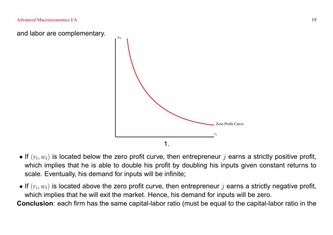
and labor are complementary.
rt
wt
Zero Pro�t Curve
1.
� If (rt; wt) is located below the zero pro�t curve, then entrepreneur j earns a strictly positive pro�t,which implies that he is able to double his pro�t by doubling his inputs given constant returns toscale. Eventually, his demand for inputs will be in�nite;
� If (rt; wt) is located above the zero pro�t curve, then entrepreneur j earns a strictly negative pro�t,which implies that he will exit the market. Hence, his demand for inputs will be zero.
Conclusion: each �rm has the same capital-labor ratio (must be equal to the capital-labor ratio in the
Advanced Macroeconomics I/A 20
economy Kt=Lt), and earns zero pro�t. Hence, �i : i 2 [0; 1] won't matter.
2.3.3 The Law of MotionAssume F (K;L;A) = F (K;AL), and At+1 = (1 + g)tA0. Then, (3) - (5) imply
Kt+1 �Zi
K it+1di =
Zi
[(1� �)K it + sY
it ]di = (1� �)Kt + sF (Kt; AtLt)
+
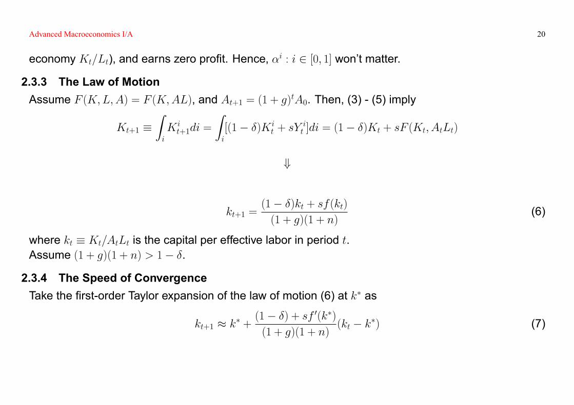
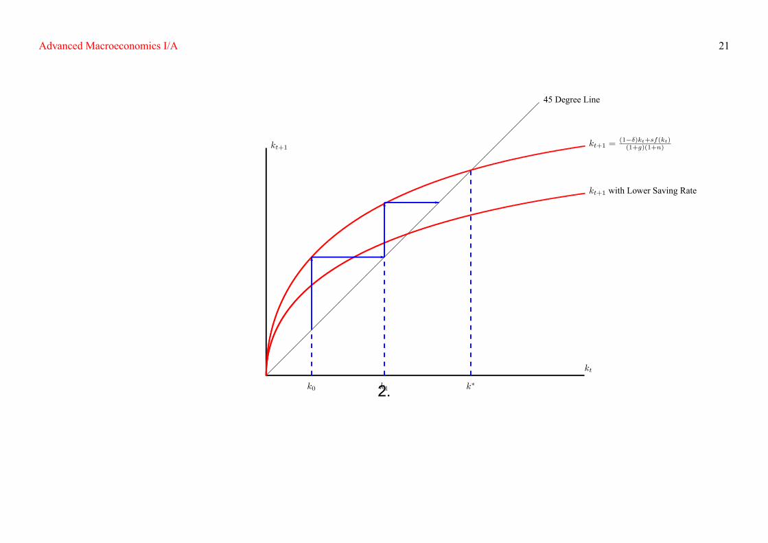
kt+1 =(1� �)kt + sf (kt)(1 + g)(1 + n)
(6)
where kt � Kt=AtLt is the capital per effective labor in period t.Assume (1 + g)(1 + n) > 1� �.
2.3.4 The Speed of ConvergenceTake the �rst-order Taylor expansion of the law of motion (6) at k� as
kt+1 � k� +(1� �) + sf 0(k�)(1 + g)(1 + n)
(kt � k�) (7)
Advanced Macroeconomics I/A 21
������������������������������
kt
kt+1
45 Degree Line
k�
kt+1 =(1��)kt+sf(kt)(1+g)(1+n)
kt+1 with Lower Saving Rate
k0 k1
6-
6-
2.
Advanced Macroeconomics I/A 22
+
kt+1 � ktkt
��1� (1� �) + sf
0(k�)
(1 + g)(1 + n)
��k�
kt� 1�
which implies convergence: given kt < k�, the growth rate of capital per effective labor decreases askt approaches k�.Remark: (7) is the tangent of (6) at k�.
2.3.5 The Golden RuleTry to choose the saving rate s to maximize the steady state consumption per effective labor c�.The steady state capital per effective labor is de�ned by
sf (k�) = [(1 + g)(1 + n)� (1� �)]k�. (8)
Then we havedk�
ds=
f (k�)
[(1 + g)(1 + n)� (1� �)]� sf 0(k�) � 0
+
Advanced Macroeconomics I/A 23
dc�
ds=d((1� s)f (k�))
ds=f (k�)ff 0(k�)� [(1 + g)(1 + n)� (1� �)]g[(1 + g)(1 + n)� (1� �)]� sf 0(k�)
+
f 0(kgold) = [(1 + g)(1 + n)� (1� �)] � g + n + �. (9)
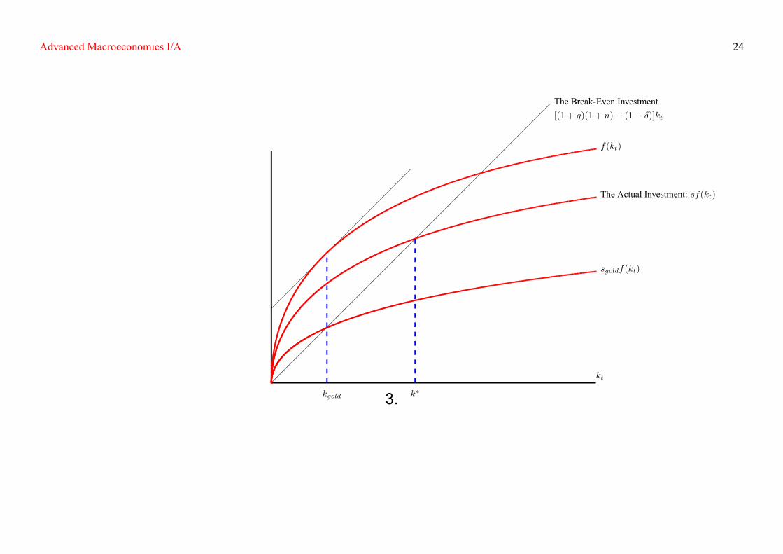
Then [(1+ g)(1+n)� (1� �)]kt is the break-even investment per effective labor, and sf (kt) is the actualinvestment per effective labor, as illustrated below.Question: higher saving rate, higher steady state capital per effective labor, but not necessarily highersteady state consumption per effective labor. Why?
2.3.6 ShocksA permanent increase/decrease in the saving rate. Then what happens to kt, ct, and Yt=Lt?
2.3.7 Dynamic Inef�ciencyLowering s when k� > kgold (as a result of s > sgold) increases consumption per effective labor in eachperiod.
2.3.8 Social Planner's ProblemThere is a dictator, or social planner, that chooses the static and intertemporal allocation of resources
Advanced Macroeconomics I/A 24
������������������������������
���������������
kt
The Break-Even Investment[(1 + g)(1 + n)� (1� �)]kt
k�kgold
f(kt)
The Actual Investment: sf(kt)
sgoldf(kt)
3.
Advanced Macroeconomics I/A 25
and dictates that allocations to the households of the economy. In each period, the social plannersaves a constant fraction s 2 [0; 1] of contemporaneous output, to be added to the economy's capitalstock, and distributes the remaining fraction uniformly across the households of the economy. Then,
Kt+1 = (1� �)Kt + sF (Kt; Lt; At)
which replicates the same allocations of the competitive economy described above. An example ofThe First Welfare Theorem.
2.3.9 Non-neoclassical Production FunctionPoverty traps, cycles, endogenous growth, etc.
2.4 References & Further Readings[1] Advanced Macroeconomics, Chapter 1. (PS2: 1.3-1.5)[2] Daron Acemoglu (2009), "Introduction to Modern Economic Growth," Princeton University Press,Chapter 1.[3] Robert Barro and Xavier Sala-i-Martin (2004), "Economic Growth," MIT Press, Chapter 1.[4] Penn World Tables http://pwt.econ.upenn.edu/php_site/pwt_index.php
Advanced Macroeconomics I/A 26
3 The Ramsey Model
3.1 Setup� Time is discrete and lasts forever indexed by t = 0; 1; � � �;
� There is a continuum of households indexed by i 2 [0; 1];
� The number of heads in each household grows at a constant rate n � 0 such that Lit = (1 + n)tLi0;
� There is a competitive supply of entrepreneurs;
� There is a consumption/investment good;
� Household i holds a �xed fraction �i of the aggregate index of stocks in the economy withR�idi = 1;
� Household i has the following preferences:1Xt=�
�t��Litu(Cit=L
it);
� Each entrepreneur has access to the same "neoclassical" production technology.
Advanced Macroeconomics I/A 27
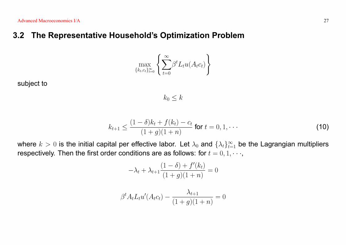
3.2 The Representative Household's Optimization Problem
maxfkt;ctg1t=0
( 1Xt=0
�tLtu(Atct)
)subject to
k0 � k
kt+1 �(1� �)kt + f (kt)� ct
(1 + g)(1 + n)for t = 0; 1; � � � (10)
where k > 0 is the initial capital per effective labor. Let �0 and f�tg1t=1 be the Lagrangian multipliersrespectively. Then the �rst order conditions are as follows: for t = 0; 1; � � �,
��t + �t+1(1� �) + f 0(kt)(1 + g)(1 + n)
= 0
�tAtLtu0(Atct)�
�t+1(1 + g)(1 + n)
= 0
Advanced Macroeconomics I/A 28
+
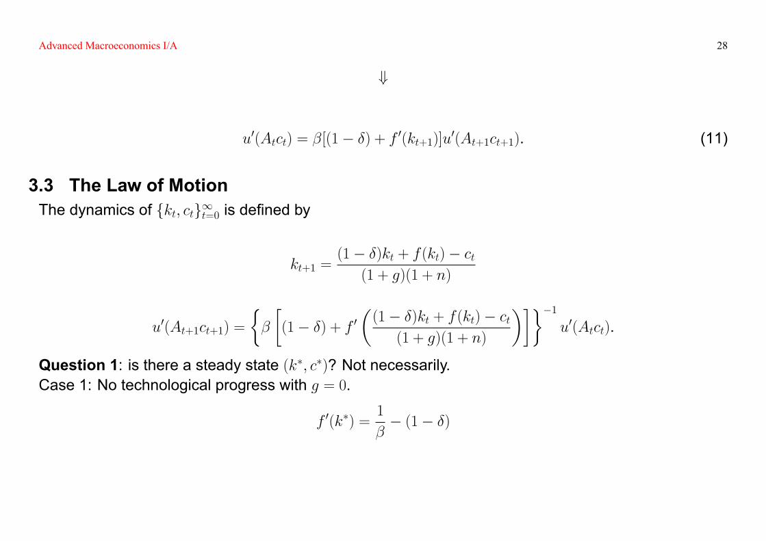
u0(Atct) = �[(1� �) + f 0(kt+1)]u0(At+1ct+1). (11)
3.3 The Law of MotionThe dynamics of fkt; ctg1t=0 is de�ned by
kt+1 =(1� �)kt + f (kt)� ct
(1 + g)(1 + n)
u0(At+1ct+1) =
��
�(1� �) + f 0
�(1� �)kt + f (kt)� ct
(1 + g)(1 + n)
����1u0(Atct).
Question 1: is there a steady state (k�; c�)? Not necessarily.Case 1: No technological progress with g = 0.
f 0(k�) =1
�� (1� �)
Advanced Macroeconomics I/A 29
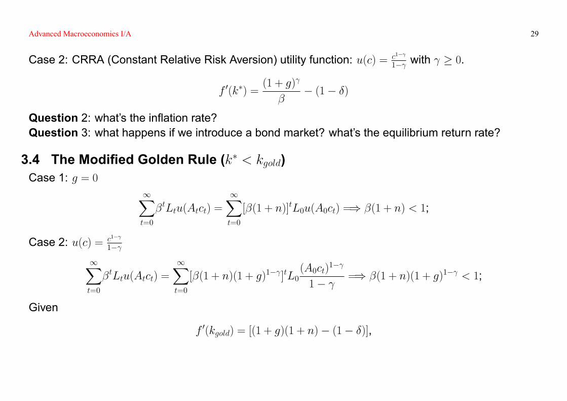
Case 2: CRRA (Constant Relative Risk Aversion) utility function: u(c) = c1�
1� with � 0.
f 0(k�) =(1 + g)
�� (1� �)
Question 2: what's the in�ation rate?Question 3: what happens if we introduce a bond market? what's the equilibrium return rate?
3.4 The Modi�ed Golden Rule (k� < kgold)Case 1: g = 0
1Xt=0
�tLtu(Atct) =
1Xt=0
[�(1 + n)]tL0u(A0ct) =) �(1 + n) < 1;
Case 2: u(c) = c1�
1�
1Xt=0
�tLtu(Atct) =1Xt=0
[�(1 + n)(1 + g)1� ]tL0(A0ct)
1�
1� =) �(1 + n)(1 + g)1� < 1;
Given
f 0(kgold) = [(1 + g)(1 + n)� (1� �)],

Advanced Macroeconomics I/A 30
then k� < kgold. Why?
3.5 Dynamics� Consider the path in the green curve above the saddle path.
� Consider the path in the green curve below the saddle path.
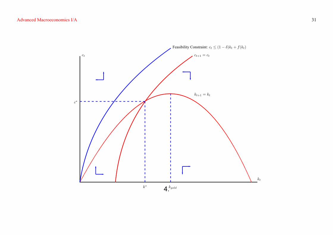
Advanced Macroeconomics I/A 31
kt
ct ct+1 = ct
kt+1 = kt
k� kgold
c�
Feasibility Constraint: ct � (1� �)kt + f(kt)
-6
-
?
�
?�6
4.
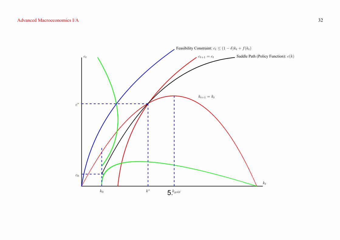
Advanced Macroeconomics I/A 32
kt
ct ct+1 = ct
kt+1 = kt
k� kgold
c�
k0
c0
Saddle Path (Policy Function): c(k)
Feasibility Constraint: ct � (1� �)kt + f(kt)
5.
Advanced Macroeconomics I/A 33
3.6 Policy Implications� Let f� tg1t=0 is the sequence of lump sum taxes per effective labor such that
kt+1 �(1� �)kt + (f (kt)� � t)� ct
(1 + g)(1 + n)for t = 0; 1; � � �;
� Assume the representative household originally expects the tax to be �xed at � each period;
� Assume the economy is in the steady state;
� Consider the following scenarios:(i) The government announces unexpectedly that the tax will be increased to � 0 > � thereafter;(ii) The government announces unexpectedly that the tax will be increased temporarily to � 0 > � forthe next ten periods;(iii) The government announces unexpectedly in period t that the tax will be increased temporarily to� 0 > � from period t + 10 to period t + 19.
3.7 Analytical vs. Numerical Analysis
3.7.1 Linear Quadratic Problem
Assume u(c) = ln c, f (k) = Ak� with � 2 (0; 1), and � = 1
Advanced Macroeconomics I/A 34
+
kt+1 =Ak�t � ct
(1 + g)(1 + n)
ct+1 =A��
1 + g
�Ak�t � ct
(1 + g)(1 + n)
���1ct
+
k� =
�A��
1 + g
� 11��
and c� = A�A��
1 + g
� �1��
� (1 + g)(1 + n)�A��
1 + g
� 11��
and
ct = [1� ��(1 + n)]Ak�t (By Guess and Verify)
+
The saving rate is �xed at ��(1 + n).
Advanced Macroeconomics I/A 35
Note: the golden-rule saving rate is � instead.
3.7.2 Numerical Algorithm
Assume u(c) =c1�
1� and f (k) = Ak�.
� Forward IterationStep 1: Given T , assume that fk0; k1; � � �; kT ; kT+1 = k�g satis�es the law of motion as follows
kt+1 =(1� �)kt + Ak�t � ct(1 + g)(1 + n)
(12)
�ct+1ct
� =��(1� �) + A�k��1t+1
�(1 + g)
(13)
for t = 0; � � �; T . Furthermore, (12) implies
ct = (1� �)kt + Ak�t � (1 + g)(1 + n)kt+1
which can be inserted into (13) such that�(1� �)kt+1 + Ak�t+1 � (1 + g)(1 + n)kt+2(1� �)kt + Ak�t � (1 + g)(1 + n)kt+1
� ���(1� �) + A�k��1t+1
�(1 + g)
= 0 (14)
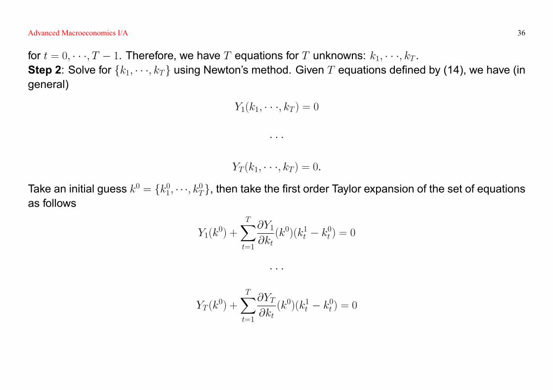
Advanced Macroeconomics I/A 36
for t = 0; � � �; T � 1. Therefore, we have T equations for T unknowns: k1; � � �; kT .Step 2: Solve for fk1; � � �; kTg using Newton's method. Given T equations de�ned by (14), we have (ingeneral)
Y1(k1; � � �; kT ) = 0
� � �
YT (k1; � � �; kT ) = 0.
Take an initial guess k0 = fk01; � � �; k0Tg, then take the �rst order Taylor expansion of the set of equationsas follows
Y1(k0) +
TXt=1
@Y1@kt
(k0)(k1t � k0t ) = 0
� � �
YT (k0) +
TXt=1
@YT@kt
(k0)(k1t � k0t ) = 0
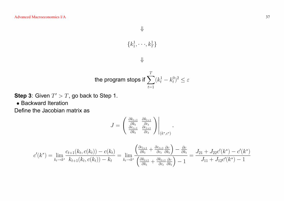
Advanced Macroeconomics I/A 37
+
fk11; � � �; k1Tg
+
the program stops ifTXt=1
(k1t � k0t )2 � "
Step 3: Given T 0 > T , go back to Step 1.� Backward IterationDe�ne the Jacobian matrix as
J =
@kt+1@kt
@kt+1@ct
@ct+1@kt
@ct+1@ct
!�����(k�;c�)
.
c0(k�) = limkt!k�
ct+1(kt; c(kt))� c(kt)kt+1(kt; c(kt))� kt
= limkt!k�
�@ct+1@kt
+ @ct+1@ct
@c@kt
�� @c
@kt�@kt+1@kt
+ @kt+1@ct
@c@kt
�� 1
=J21 + J22c
0(k�)� c0(k�)J11 + J12c0(k�)� 1
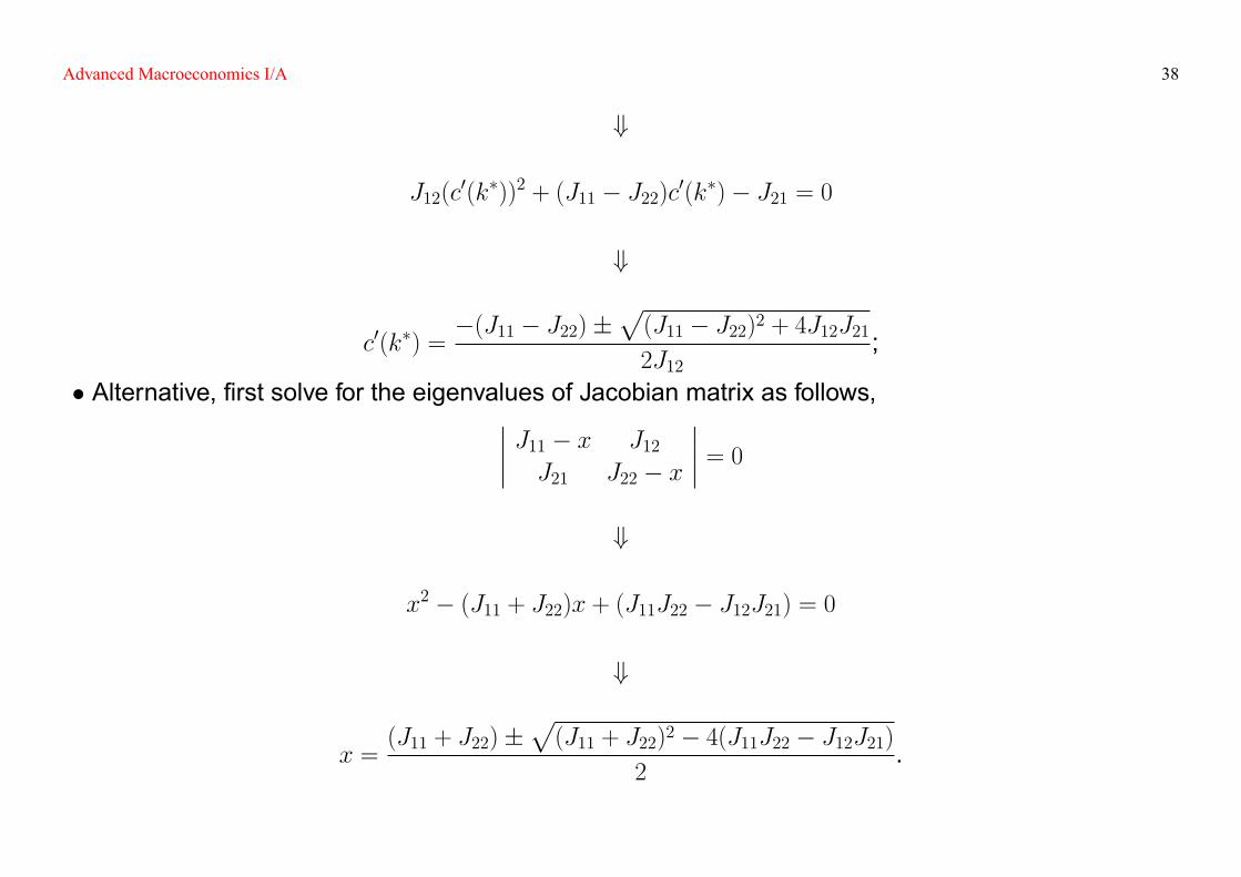
Advanced Macroeconomics I/A 38
+
J12(c0(k�))2 + (J11 � J22)c0(k�)� J21 = 0
+
c0(k�) =�(J11 � J22)�
p(J11 � J22)2 + 4J12J212J12
;
� Alternative, �rst solve for the eigenvalues of Jacobian matrix as follows,���� J11 � x J12J21 J22 � x
���� = 0+
x2 � (J11 + J22)x + (J11J22 � J12J21) = 0
+
x =(J11 + J22)�
p(J11 + J22)2 � 4(J11J22 � J12J21)
2.
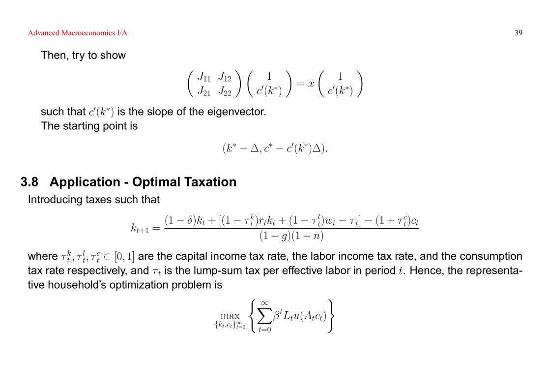
Advanced Macroeconomics I/A 39
Then, try to show �J11 J12J21 J22
��1
c0(k�)
�= x
�1
c0(k�)
�such that c0(k�) is the slope of the eigenvector.The starting point is
(k� ��; c� � c0(k�)�).
3.8 Application - Optimal TaxationIntroducing taxes such that
kt+1 =(1� �)kt + [(1� � kt )rtkt + (1� � lt)wt � � t]� (1 + � ct)ct
(1 + g)(1 + n)
where � kt ; � lt; � ct 2 [0; 1] are the capital income tax rate, the labor income tax rate, and the consumptiontax rate respectively, and � t is the lump-sum tax per effective labor in period t. Hence, the representa-tive household's optimization problem is
maxfkt;ctg1t=0
( 1Xt=0
�tLtu(Atct)
)
Advanced Macroeconomics I/A 40
subject to
k0 � k
kt+1 �(1� �)kt + [(1� � kt )rtkt + (1� � lt)wt � � t]� (1 + � ct)ct
(1 + g)(1 + n)for t = 0; 1; � � �
where k > 0 is the initial capital per effective labor. Let �0 and f�tg1t=1 be the Lagrangian multipliersrespectively. Then the �rst order conditions are as follows: for t = 0; 1; � � �,
��t + �t+1(1� �) + (1� � kt )rt(1 + g)(1 + n)
= 0
�tAtLtu0(Atct)�
�t+1(1 + �ct)
(1 + g)(1 + n)= 0
+
u0(Atct)
1 + � ct= �[(1� �) + (1� � kt+1)rt+1)]
u0(At+1ct+1)
1 + � ct+1
+
Advanced Macroeconomics I/A 41�ct+1ct
� =�[(1� �) + (1� � kt+1)rt+1)]
(1 + g) 1 + � ct1 + � ct+1
The government's budget constraint is
� kt rtkt + �ltwt + � t + �
ctct = Gt
where Gt is the government expenditure per effective labor in period t. And, in the equilibrium,
rt = f0(kt) and wt = f (kt)� f 0(kt)kt.
Question: Advanced Macroeconomics, 2.9Question: Finance a �xed government expenditure G each period by the capital income tax, or thelabor income tax, or the lump sum tax, or the consumption tax. What are the different implications?
3.9 References & Further Readings[1] Advanced Macroeconomics, Chapter 2;[2] Get Started with MATLAB.
Advanced Macroeconomics I/A 42
4 Equilibrium with Complete Markets
4.1 Setup� Time is discrete and lasts forever indexed by t = 0; 1; � � �;
� There are I agents indexed by i = 1; 2; � � �; I;
� There is a non-storable consumption good;
� There is a stochastic event st 2 S in period t;
� The history of events up to period t is st � (s0; s1; � � �; st) 2 St+1;
� Let �t(st) 2 [0; 1] be the unconditional probability of the history st with
�0(s0) = 1 and
Xst2St+1
�t(st) = 1 for all t;
� Let yit(st) � 0 be agent i's endowment in period t conditional on the history st;
� Agent i has the following preferences:1Xt=0
�t
Xst2St+1
�t(st)u(cit(s
t))
!.
Advanced Macroeconomics I/A 43
4.2 Pareto ProblemAn allocation: cit(st) � 0 for all i; t; st is feasible if
IXi=1
cit(st) �
IXi=1
yit(st) for all t = 0; 1; � � � and for all st 2 St+1.
Let �1; �1; � � �; �I � 0 be the Pareto weights. Thus, the social planner's optimization problem is
maxcit(s
t) for all i, t, st
(IXi=1
�i
1Xt=0
Xst2St+1
�t�t(st)u(cit(s
t))
!)subject to
IXi=1
cit(st) �
IXi=1
yit(st) for all t = 0; 1; � � � and for all st 2 St+1
Let �t(st) be the Lagrangian multiplier for the feasibility constraint in period t conditional on the historyst. Then, the �rst order condition is
�i�t�t(s
t)u0(cit(st))� �t(st) = 0
+
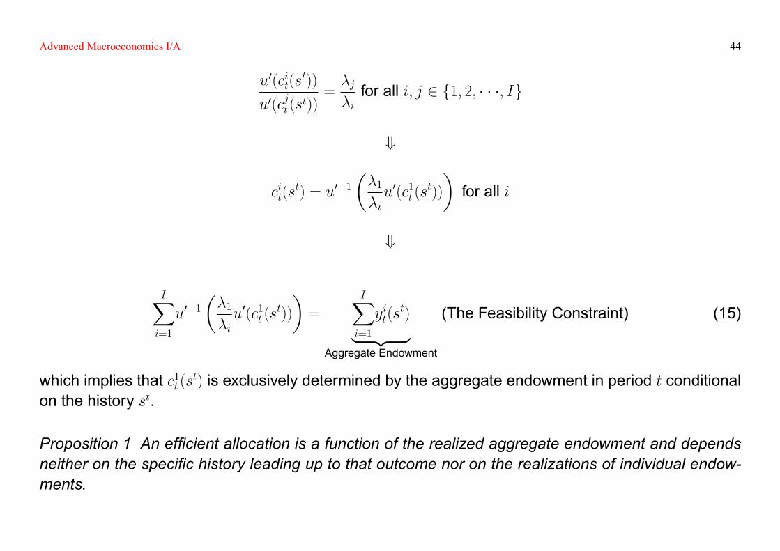
Advanced Macroeconomics I/A 44
u0(cit(st))
u0(cjt(st))=�j�ifor all i; j 2 f1; 2; � � �; Ig
+
cit(st) = u0�1
��1�iu0(c1t (s
t))
�for all i
+
IXi=1
u0�1��1�iu0(c1t (s
t))
�=
IXi=1
yit(st)| {z }
Aggregate Endowment
(The Feasibility Constraint) (15)
which implies that c1t (st) is exclusively determined by the aggregate endowment in period t conditionalon the history st.
Proposition 1 An ef�cient allocation is a function of the realized aggregate endowment and dependsneither on the speci�c history leading up to that outcome nor on the realizations of individual endow-ments.
Advanced Macroeconomics I/A 45
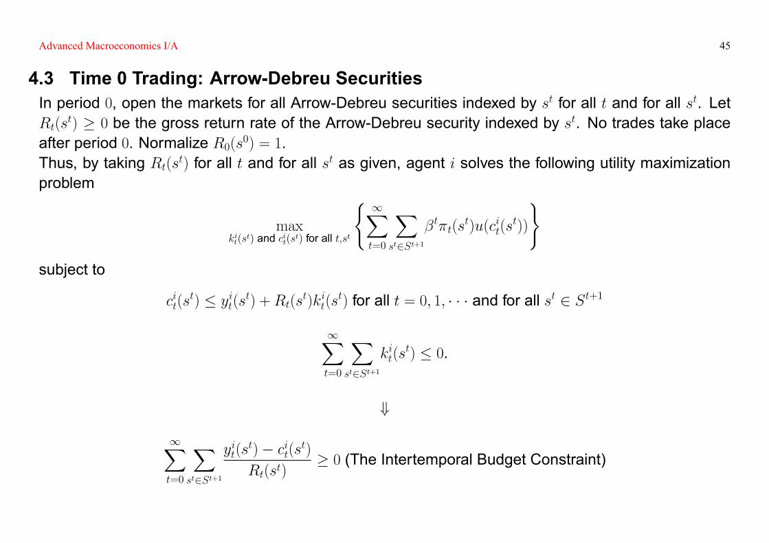
4.3 Time 0 Trading: Arrow-Debreu SecuritiesIn period 0, open the markets for all Arrow-Debreu securities indexed by st for all t and for all st. LetRt(s
t) � 0 be the gross return rate of the Arrow-Debreu security indexed by st. No trades take placeafter period 0. Normalize R0(s0) = 1.Thus, by taking Rt(st) for all t and for all st as given, agent i solves the following utility maximizationproblem
maxkit(s
t) and cit(st) for all t;st
( 1Xt=0
Xst2St+1
�t�t(st)u(cit(s
t))
)subject to
cit(st) � yit(st) +Rt(st)kit(st) for all t = 0; 1; � � � and for all st 2 St+1
1Xt=0
Xst2St+1
kit(st) � 0.
+
1Xt=0
Xst2St+1
yit(st)� cit(st)Rt(st)
� 0 (The Intertemporal Budget Constraint)
Advanced Macroeconomics I/A 46
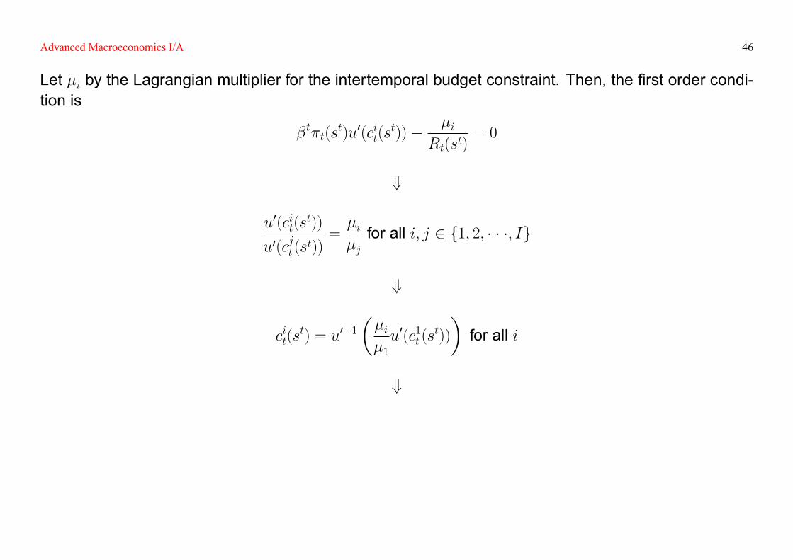
Let �i by the Lagrangian multiplier for the intertemporal budget constraint. Then, the �rst order condi-tion is
�t�t(st)u0(cit(s
t))� �iRt(st)
= 0
+
u0(cit(st))
u0(cjt(st))=�i�jfor all i; j 2 f1; 2; � � �; Ig
+
cit(st) = u0�1
��i�1u0(c1t (s
t))
�for all i
+
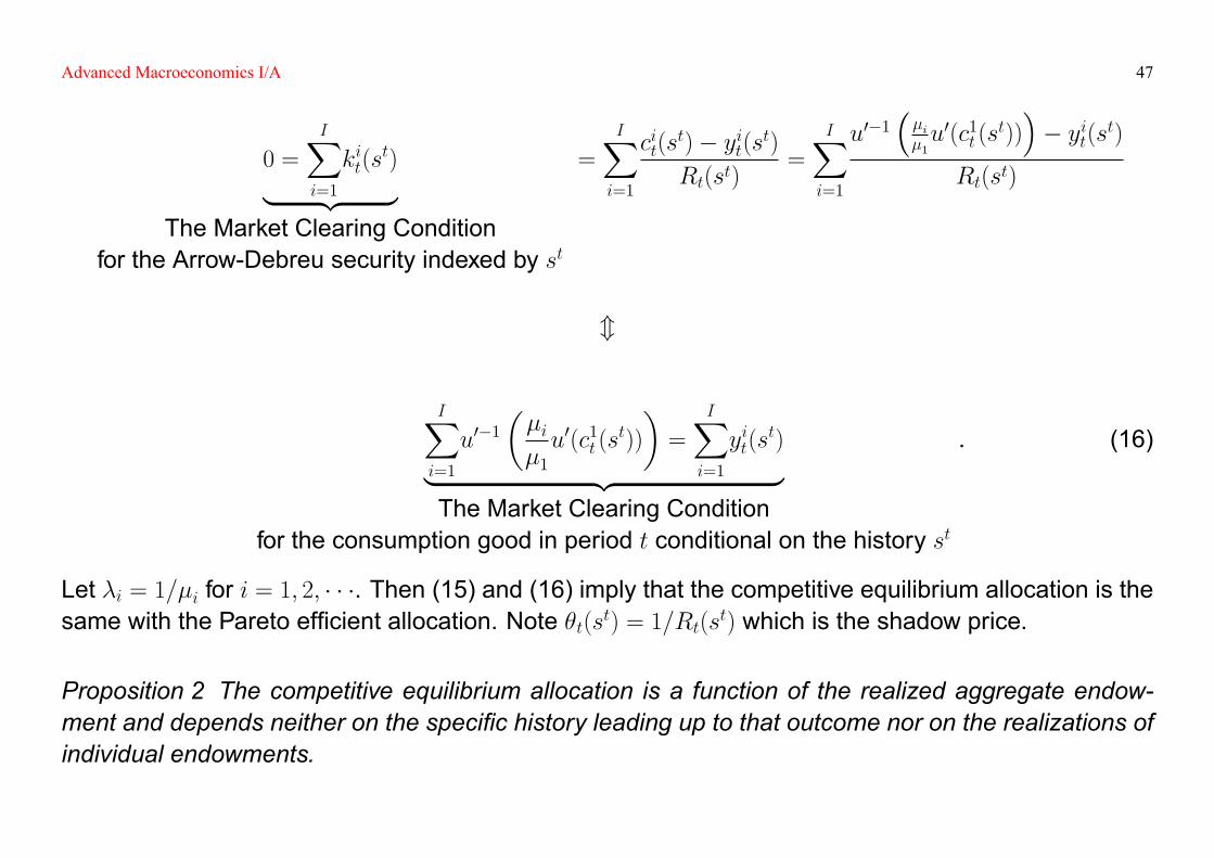
Advanced Macroeconomics I/A 47
0 =
IXi=1
kit(st)| {z }
The Market Clearing Conditionfor the Arrow-Debreu security indexed by st
=
IXi=1
cit(st)� yit(st)Rt(st)
=
IXi=1
u0�1��i�1u0(c1t (s
t))�� yit(st)
Rt(st)
m
IXi=1
u0�1��i�1u0(c1t (s
t))
�=
IXi=1
yit(st)| {z }
The Market Clearing Conditionfor the consumption good in period t conditional on the history st
. (16)
Let �i = 1=�i for i = 1; 2; � � �. Then (15) and (16) imply that the competitive equilibrium allocation is thesame with the Pareto ef�cient allocation. Note �t(st) = 1=Rt(st) which is the shadow price.
Proposition 2 The competitive equilibrium allocation is a function of the realized aggregate endow-ment and depends neither on the speci�c history leading up to that outcome nor on the realizations ofindividual endowments.
Advanced Macroeconomics I/A 48
Remark 1: No Aggregate Uncertainty
AssumeIPi=1
yit(st) = Y for all t and for all st. Then, agent i's optimal consumption is �xed at ci with
ci = (1� �)1Xt=0
Xst2St+1
�t�t(st)yit(s
t)| {z }The Permanent Income
.
Note: Rt(st) = 1�t�t(st)
such that the gross return rate of a T -period risk free bond is 1�t.
Remark 2: Asset PricingAssume the return function of an asset is Rt(st) for all t and for all st. Then, the price should be
P =
1Xt=0
Xst2St+1
Rt(st)
Rt(st).
Remark 3: Time ConsistencyGiven � and s� , reopen the markets for the Arrow-Debreu securities indexed by st j s� for all t � � andfor all st j s� . Then, for i = 1; 2; � � �; I,
maxkit(s
tjs� ) and cit(stjs� ) for all t�� ;stjs�
8<:1Xt=�
Xstjs�2St+1
�t���t(s
t)
�� (s� )u(cit(s
t j s� ))
9=;
Advanced Macroeconomics I/A 49
subject to
cit(st j s� ) � yit(st) +Rt(st)kit(st j s� ) for all t � � and for all st j s� 2 St+1
1Xt=�
Xstjs�2St+1
Pt(st j s� )kit(st j s� ) �
1Xt=�
Xstjs�2St+1
Pt(st j s� )kit(st).
+
1Xt=�
Xstjs�2St+1
Pt(st j s� )c
it(s
t j s� )� yit(st)Rt(st)
�1Xt=�
Xstjs�2St+1
Pt(st j s� )kit(st) (the Intertemporal Budget Constraint)
+
�t���t(s
t)
�� (s� )u0(cit(s
t j s� ))� �i(s� )Pt(s
t j s� )Rt(st)
= 0 (the First Order Condition)
Question: It is possible kit(st j s� ) 6= kit(st) (or equivalently, cit(st j s� ) 6= cit(st))?Note: Pt(st j s� ) = R� (s� ) and �i(s� ) = �i
���� (s� )R� (s� )
Advanced Macroeconomics I/A 50
4.4 Sequential Trading: Arrow SecuritiesIn period t conditional on the history st, only open the markets for the Arrow securities indexed byst+1 j st with the gross return rate eRt+1(st+1).Given the competitive equilibrium as derived above, de�ne
ai0(s0) =
1Xt=0
Xst2St+1
cit(st)� yit(st)Rt(st)
as agent i's initial asset. Then,
ci0(s0) +
Xs12S
ai1(s0; s1) � yi0(s0) + ai0(s0)
+
cit(st) +
Xst+12S
ait+1(st; st+1) � yit(st) + eRt(st)ait(st) for all t and for all st.
The corresponding optimization problem is
maxait(s
t) and cit(st) for all t;st
( 1Xt=0
Xst2St+1
�t�t(st)u(cit(s
t))
)
Advanced Macroeconomics I/A 51
subject to
ai0(s0) �
1Xt=0
Xst2St+1
cit(st)� yit(st)Rt(st)
cit(st) +
Xst+12S
ait+1(st; st+1) � yit(st) + eRt(st)ait(st) for all t and for all st. (17)
If we try to solve the above problem directly, the solution is a Ponzi scheme with ait(st) = �1. There-fore, we add the following debt limit condition
ait(st) �
24�Rt(st)0@ 1X�=t
Xs� jst2S�+1
yi� (s� )
R� (s� )
1A35, eRt(st) for all t and for all st. (18)
Let �it(st) and �it(st) be the Lagrangian multipliers for (17) and (18) respectively. Then, the �rst orderconditions are
��it�1(st�1) + �it(st) eRt(st) + �it(st) = 0�t�t(s
t)u0(cit(st))� �it(st) = 0
Advanced Macroeconomics I/A 52
+
�it(st) = 0 for all t and for all st
Hence, suppose
ai0(s0) = 0 for all i
�it(st) =
�iRt(st)
and eRt(st) = Rt(st)
Rt�1(st�1)for all t and for all st.
Then, once again, we have the same allocation.Question: Recursive Macroeconomic Theory, 8.1, 8.3, and 8.4(Part I).
4.5 References & Further Readings[1] Recursive Macroeconomic Theory, Chapter 8;
Advanced Macroeconomics I/A 53
5 Dynamic Programming
5.1 A Deterministic Example� Time is discrete and lasts for T + 1 periods indexed by t = 0; 1; � � �; T ;
� There is a bond with the gross return rate 1 + r.
V �0 (a0) = maxfat+1;ctgTt=0
(TXt=0
�tu(ct)
)subject to
at+1 = (1 + r)(at � ct) for t = 0; 1; � � �; T
aT+1 � 0.
Try to solve the problem backward as follows
V �T (aT ) = u(aT )
+
Advanced Macroeconomics I/A 54
V �T�1(aT�1) = maxaT ;cT�1
fu(cT�1) + �V �T (aT )g subject to aT = (1 + r)(aT�1 � cT�1)
+
� � �
Remark: T could be in�nity.
5.2 A Stochastic Example� Time is discrete and lasts for T + 1 periods indexed by t = 0; 1; � � �; T ;
� There are a bond with the gross return rate 1, and a stock with the stochastic gross return R 2 [R;R]which is drawn each period independently from a given distribution.
V �0 (w0) = max
(TXt=0
�t�Z
Rtu(ct(R
t))f (R0) � � � f (Rt)dRt�)
subject to
wt+1(Rt) = Rtst(R
t�1) + (wt(Rt�1)� st(Rt�1))� ct(Rt) for all Rt and all t
wT+1(RT ) � 0 for all RT .
Advanced Macroeconomics I/A 55
Try to solve the problem backward by assuming u(c) = c1�
1� and � = 1 as follows
VT (w) = maxs2[0;w]
�ZR
(Rs + (w � s))1� 1� dF (R)
�= �
w1�
1� where
� � max�2[0;1]
�ZR
(R� + (1� �))1� dF (R)�.
+
VT�1(w) = maxs;c(R):R2[R;R]
(Z R
R
�(c(R))1�
1� + �(Rs + (w � s)� c(R))1�
1�
�dF (R)
)= �2(1 + ��
1 ) w1�
1�
+
� � �
5.3 A General Recursive Problem - Deterministic� Time is discrete and lasts forever indexed by t = 0; 1; � � �;
Advanced Macroeconomics I/A 56
� The discount factor is � 2 (0; 1);
� The state variable xt 2 X;
� The constraint correspondence � : X ! 2X such that xt+1 2 �(xt);
� The payoff function F (xt; xt+1) de�ned for all xt 2 X and all xt+1 2 �(xt);
� A plan from x0 is a sequence fxtg1t=0;
� A feasible plan from x0 is a sequence fxtg1t=0 with xt+1 2 �(xt) for all t = 0; 1; � � �;
The Original Problem
V �(x0) = maxfxt+1g1t=0
( 1Xt=0
�tF (xt; xt+1)
)subject to xt+1 2 �(xt) for t = 0; 1; � � �; (19)
The Recursive Problem
V (x) = maxx0fF (x; x0) + �V (x0)g subject to x0 2 �(x). (20)
Advanced Macroeconomics I/A 57
Remark: (20) is called a functional equation in which a solution means a function V : X ! R.
Question 1: Is V � a solution for the functional equation (20)?Answer: Yes.Proof: Take any x0 2 X as given. It suf�ces to show that exists x�1 2 �(x0) such that
V �(x0) = F (x0; x�1) + �V
�(x�1) � F (x0; x1) + �V �(x1) for all x1 2 �(x0).
Let fx�tg1t=0 be an optimal plan from x0. Then,
V �(x0) = F (x0; x�1) + �
1Xt=1
�t�1F (x�t ; x�t+1) � F (x0; x1) + �V �(x1) for all x1 2 �(x0)
where the equality follows the de�nition of V �, and the inequality follows the fact that given any x1 2�(x0), if fx��t g1t=1 is an optimal plan from x1, then fx0; x1; x��2 ; � � �g is a feasible plan from x0.Furthermore, the inequality above implies
1Xt=1
�t�1F (x�t ; x�t+1) � V �(x�1)
by taking x1 = x�1. Note that the equality must hold given the de�nition of V �(x1).
Advanced Macroeconomics I/A 58
The result follows.
Question 2: Is V � the only solution for the functional equation (20)?Answer: Not necessarily.Counterexample: Assume F (x; x0) = x � �x0, X = R, �(x) = f���1xg if x > 0, and �(x) = f��1xgif x � 0. Then, for any x, there exists only one feasible plan such that V �(x) = maxf2x; 0g. However,there exists another solution V (x) = x for the functional equation
V (x) = maxf(x� �x0) + �V (x0)g subject to x0 2 �(x).
Question 3: De�ne the policy correspondence
G(x) = argmaxx0
fF (x; x0) + �V �(x0)g subject to x0 2 �(x).
Therefore, if fx�tg1t=0 is an optimal plan from x0, then
x�t+1 2 G(x�t ) for all t = 0; 1; � � �.
Answer: Yes.Proof: To be completed.
Advanced Macroeconomics I/A 59
Question 4: Is any plan fxtg1t=0 with xt+1 2 G(xt) for all t = 0; 1; � � � an optimal plan from x0?Answer: Not necessarily. Furthermore, the answer is yes if and only if lim
t!1�tV �(xt) = 0.
Counterexample: Assume F (x; x0) = x � �x0, X = R+, and �(x) = [0; ��1x]. It is straightforward toshow V �(x) = x. Therefore, the policy correspondence is
G(x) = argmaxx02[0;��1x]
f(x� �x0) + �V �(x0)g = [0; ��1x].
However, the policy correspondence is able to generate a plan from x with c = 0 for all t, which is notoptimal because the agent is not willing to postpone consumption forever.Proof: Given fx�tg1t=0 with x�t+1 2 G(x�t ) for all t = 0; 1; � � �, we have
V �(x�t ) = F (x�t ; x
�t+1) + �V
�(x�t+1) for all t
which implies
V �(x0) =TXt=0
�tF (x�t ; x�t+1) + �
T+1V �(x�T+1)
Advanced Macroeconomics I/A 60
which implies
V �(x0) = limT!1
TXt=0
�tF (x�t ; x�t+1)
!+ limT!1
�T+1V �(x�T+1).
5.4 Solving the Functional Equation
5.4.1 Assumptions� X is a convex subset of Rl;
� F (x; x0) is continuous and bounded;
� The constraint correspondence � : X ! 2X is nonempty, compact-valued, and continuous.
Remarks:� � is nonempty if �(x) is not an empty set for all x 2 X;
� � is compact-valued if �(x) is a compact subset of X for all x 2 X;
� � is continuous if � is both lower hemi-continuous and upper hemi-continuous;
� � is lower hemi-continuous at x if for every x0 2 �(x) and every sequence fxng1n=1 ! x, there exists
Advanced Macroeconomics I/A 61
a sequence fx0ng1n=1 such that limn!1
x0n = x0 and x0n 2 �(xn);
� � is upper hemi-continuous at x if for every sequence fxng1n=1 ! x and fx0n 2 �(xn)g1n=1, there existsa convergent subsequence of fx0ng1n=1 whose limit point is in �(x).
De�ne C(X) as the space of bounded continuous functions V : X ! R with the sup norm. Hence,T : C(X)! C(X) is a mapping de�ned as
TV (x) = maxx02�(x)
fF (x; x0) + �V (x0)g.
A solution for the functional equation is a �xed point of the mapping T .
5.5 The Solution for the Functional Equation is Unique� The mapping T : C(X)! C(X) is a contraction with modulus � 2 (0; 1) if
supx2X
jTV (x)� TV 0(x)j � �supx2X
jV (x)� V 0(x)j for all V; V 0 2 C(X).
� (Blackwell's Suf�cient Conditions for a Contraction) The mapping T : C(X) ! C(X) is acontraction if (i) (monotonicity) for every V; V 0 2 C(X) with V (x) � V 0(x) for all x 2 X, TV (x) �
Advanced Macroeconomics I/A 62
TV 0(x) for all x 2 X; (ii) (discounting) there exists � 2 (0; 1) such that T (V + a)(x) � TV (x) + �a forall V 2 C(X), a � 0, and x 2 X.
Proof:
V (x) � V 0(x) + kV � V 0k1 for all x 2 X
+
TV (x) � TV 0(x) + � kV � V 0k1 for all x 2 X (by monotonicity and discounting)
TV 0(x) � TV (x) + � kV � V 0k1 for all x 2 X (by monotonicity and discounting)
+
kTV � TV 0k1 � � kV � V 0k1
+
T is a contraction by de�nition
� (Contraction Mapping Theorem) Given the complete metric space (C(X); k�k1), if T is a contrac-
Advanced Macroeconomics I/A 63
tion with modulus � 2 (0; 1), then there exists exactly one �xed point in C(X).Proof: Given any V 2 C(X), de�ne the sequence fVng1n=0 with Vn = T nV . Since T is a contraction,we have
kVn+1 � Vnk1 = kTVn � TVn�1k1 � � kVn � Vn�1k1 for n = 1; 2; � � �
Thus, for m > n,
kVm � Vnk1 � kVm � Vm�1k1 + � � � + kVn+1 � Vnk1 (triangle inequality)� (�m�1 + � � � + �n) kV1 � V0k1� �n
1� � kV1 � V0k1 ! 0 as n!1
which implies fVng1n=0 is a Cauchy sequence in a complete metric space. Hence, fVng1n=0 ! V 2 C(X)which implies a �xed point exists.How to prove V is unique?
5.6 V is monotonic� F (x; x0) is increasing in its �rst l arguments;
� � is monotone in the sense that
�(x) � �(x) if x � x.
Advanced Macroeconomics I/A 64
Then V as a �xed point of T is increasing in x.Proof: It suf�ces to show that if V is increasing in x, then TV is increasing in x.Suppose V is increasing in x. Given any x1; x2 2 X with x1 � x2, let
x01 2 argmaxx02�(x1)
fF (x1; x0) + �V (x0)g.
Then given � is monotone as de�ned above, x01 2 �(x1) � �(x2) which implies
TV (x2) = maxx02�(x2)
fF (x2; x0) + �V (x0)g � F (x2; x01) + �V (x01) � F (x1; x01) + �V (x01) = TV (x1).
Hence, TV is increasing in x.
5.7 V is concave� F (x; x0) is concave;
� � is convex in the sense that if x01 2 �(x1) and x02 2 �(x2), then
�x01 + (1� �)x02 2 �(�x1 + (1� �)x2) for all � 2 [0; 1].
Then V as a �xed point of T is concave in x.Proof: It suf�ces to show that if V is concave in x, then TV is concave in x.
Advanced Macroeconomics I/A 65
Suppose V is concave in x. Given any x1; x2 2 X with x1 � x2, let
x01 2 argmaxx02�(x1)
fF (x1; x0) + �V (x0)g � �(x1)
x02 2 argmaxx02�(x2)
fF (x2; x0) + �V (x0)g � �(x2).
Since � is convex as de�ned above,
�x01 + (1� �)x02 2 �(�x1 + (1� �)x2) for all � 2 [0; 1]
which implies
TV (�x1 + (1� �)x2) = maxx02�(�x1+(1��)x2)
fF (�x1 + (1� �)x2; x0) + �V (x0)g
� F (�x1 + (1� �)x2; �x01 + (1� �)x02) + �V (�x01 + (1� �)x02)� �(F (x1; x
01) + �V (x
01)) + (1� �)(F (x2; x02) + �V (x02))
= �TV (x1) + (1� �)TV (x2)
which implies TV is concave.
5.8 V is differentiable� F (x; x0) is differentiable in the �rst l arguments;
Advanced Macroeconomics I/A 66
� V is concave;
� x 2 intX, x0 2 G(x), and x0 2 int�(x).Then V is differentiable at x.Proof: To be completed.
5.9 A Stochastic Example - Search Theory� Time is discrete and lasts forever indexed by t = 0; 1; � � �;
� There is an unemployed worker who is risk neutral;
� The unemployed worker draws a wage offer each period from a distribution F : [0; w] ! [0; 1], anddecides whether to accept the offer and stop the search.
The mapping T :h0; w1��
i!h0; w1��
iis de�ned as
T (V U) =
Z w
0
max
�w
1� � ; �VU
�dF (w) =
Z �(1��)V U
0
�V UdF (w) +
Z w
�(1��)V U
w
1� �dF (w)
+
Advanced Macroeconomics I/A 67
T 0(V U) = �F (�(1� �)V U) � �
+
T is a contraction
Question 1: what happens to V U if � increases? why?
Question 2: what happens to V U if there is a �rst-order stochastic shift in the distribution F? why?� The distribution F dominates the distribution G in the sense of 1st order stochastic dominance ifZ
h(x)dF (x) �Zh(x)dG(x)
for all monotone functions h : R! R.
Question 3: what happens to V U if there is a second-order stochastic shift in the distribution F? why?� The distribution F dominates the distribution G in the sense of 2nd order stochastic dominance ifZ
h(x)dF (x) �Zh(x)dG(x)

Advanced Macroeconomics I/A 68
for all convex functions h : R! R.
Question 4: Let's introduce the exogenous job separation probability � 2 [0; 1].
V (w) = w + �(�V U + (1� �)V (w))
V U =
Z w
0
maxfV (w); �V UgdF (w)
+
T (V U) =
Z w
0
max
�w + ��V U
1� �(1� �); �VU
�dF (w)
Try to show T is again a contraction.
5.10 A General Recursive Problem - Stochastic
5.10.1 Assumptions� X is a convex subset of Rl;
Advanced Macroeconomics I/A 69
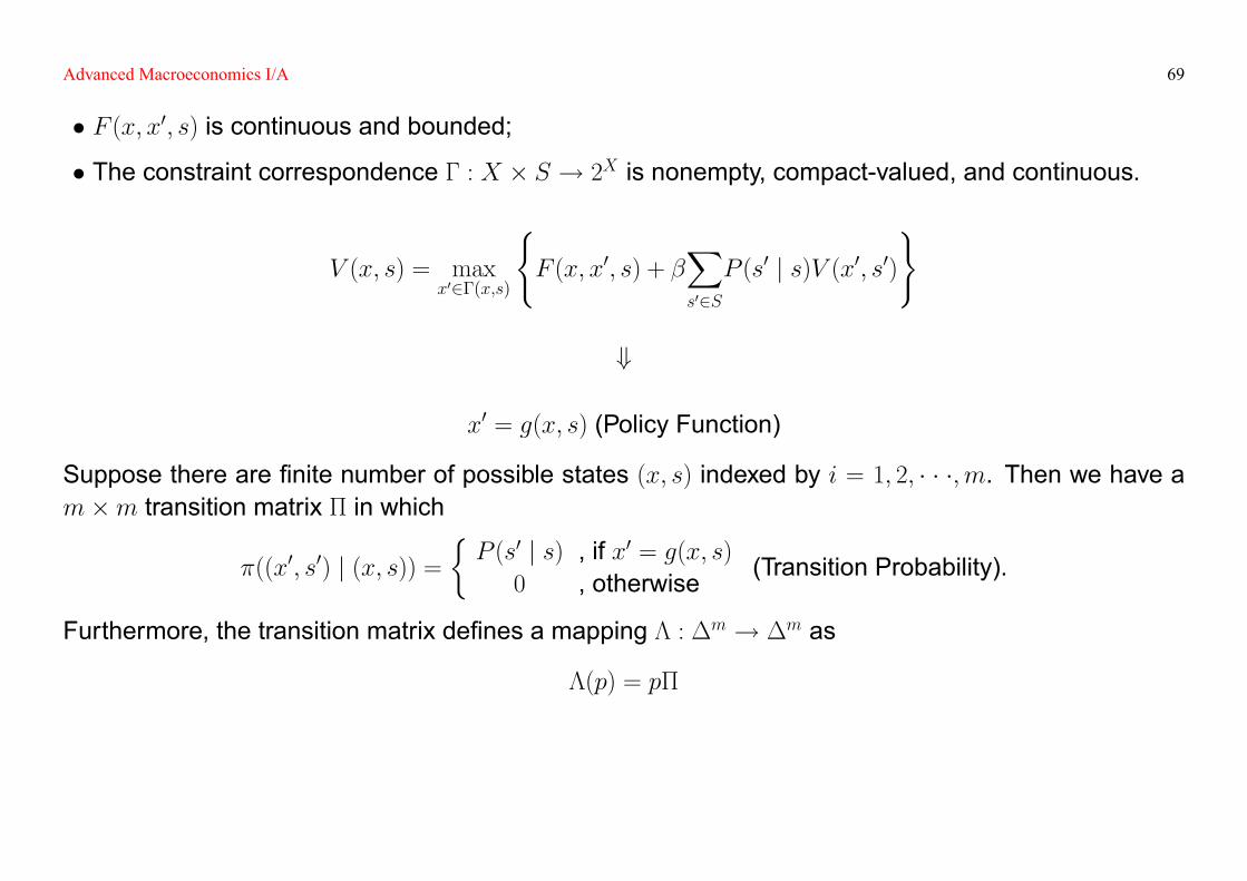
� F (x; x0; s) is continuous and bounded;
� The constraint correspondence � : X � S ! 2X is nonempty, compact-valued, and continuous.
V (x; s) = maxx02�(x;s)
(F (x; x0; s) + �
Xs02SP (s0 j s)V (x0; s0)
)
+
x0 = g(x; s) (Policy Function)
Suppose there are �nite number of possible states (x; s) indexed by i = 1; 2; � � �;m. Then we have am�m transition matrix � in which
�((x0; s0) j (x; s)) =�P (s0 j s) , if x0 = g(x; s)0 , otherwise (Transition Probability).
Furthermore, the transition matrix de�nes a mapping � : �m ! �m as
�(p) = p�
Advanced Macroeconomics I/A 70
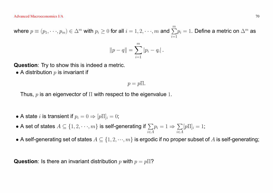
where p � (p1; � � �; pm) 2 �m with pi � 0 for all i = 1; 2; � � �;m andmPi=1
pi = 1. De�ne a metric on �m as
kp� qk =mXi=1
jpi � qij .
Question: Try to show this is indeed a metric.� A distribution p is invariant if
p = p�.
Thus, p is an eigenvector of � with respect to the eigenvalue 1.
� A state i is transient if pi = 0) [p�]i = 0;
� A set of states A � f1; 2; � � �;mg is self-generating ifPi2Api = 1)
Pi2A[p�]i = 1;
� A self-generating set of states A � f1; 2; ���;mg is ergodic if no proper subset of A is self-generating;
Question: Is there an invariant distribution p with p = p�?
Advanced Macroeconomics I/A 71
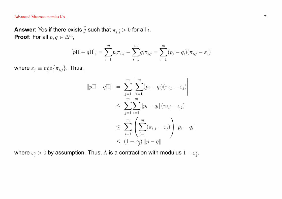
Answer: Yes if there exists bj such that �i;bj > 0 for all i.Proof: For all p; q 2 �m,
[p�� q�]j =mXi=1
pi�i;j �mXi=1
qi�i;j =
mXi=1
(pi � qi)(�i;j � "j)
where "j � minif�i;jg. Thus,
kp�� q�k =mXj=1
�����mXi=1
(pi � qi)(�i;j � "j)�����
�mXj=1
mXi=1
jpi � qij (�i;j � "j)
�mXi=1
0@ mXj=1
(�i;j � "j)
1A jpi � qij� (1� "bj) kp� qk
where "bj > 0 by assumption. Thus, � is a contraction with modulus 1� "bj.
Advanced Macroeconomics I/A 72
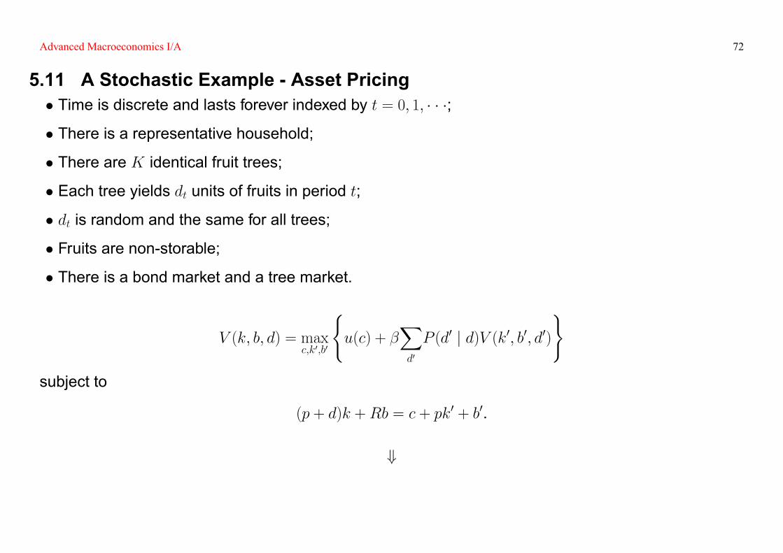
5.11 A Stochastic Example - Asset Pricing� Time is discrete and lasts forever indexed by t = 0; 1; � � �;
� There is a representative household;
� There are K identical fruit trees;
� Each tree yields dt units of fruits in period t;
� dt is random and the same for all trees;
� Fruits are non-storable;
� There is a bond market and a tree market.
V (k; b; d) = maxc;k0;b0
(u(c) + �
Xd0
P (d0 j d)V (k0; b0; d0))
subject to
(p + d)k +Rb = c + pk0 + b0.
+
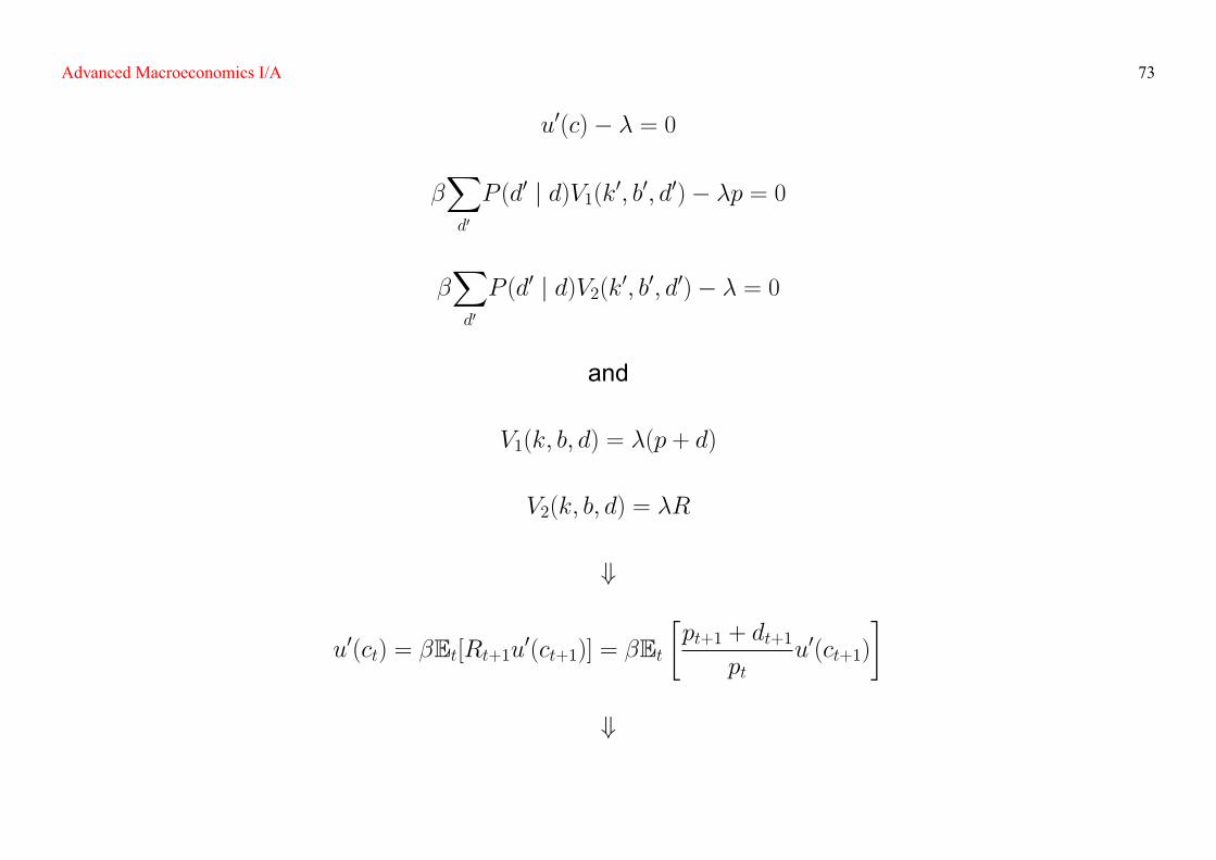
Advanced Macroeconomics I/A 73
u0(c)� � = 0
�Xd0
P (d0 j d)V1(k0; b0; d0)� �p = 0
�Xd0
P (d0 j d)V2(k0; b0; d0)� � = 0
and
V1(k; b; d) = �(p + d)
V2(k; b; d) = �R
+
u0(ct) = �Et[Rt+1u0(ct+1)] = �Et�pt+1 + dt+1
ptu0(ct+1)
�+
Advanced Macroeconomics I/A 74
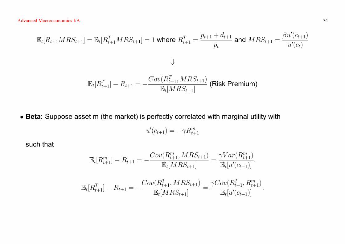
Et[Rt+1MRSt+1] = Et[RTt+1MRSt+1] = 1 where RTt+1 =pt+1 + dt+1
ptandMRSt+1 =
�u0(ct+1)
u0(ct)
+
Et[RTt+1]�Rt+1 = �Cov(RTt+1;MRSt+1)
Et[MRSt+1](Risk Premium)
� Beta: Suppose asset m (the market) is perfectly correlated with marginal utility with
u0(ct+1) = � Rmt+1such that
Et[Rmt+1]�Rt+1 = �Cov(Rmt+1;MRSt+1)
Et[MRSt+1]= V ar(Rmt+1)
Et[u0(ct+1)].
Et[RTt+1]�Rt+1 = �Cov(RTt+1;MRSt+1)
Et[MRSt+1]= Cov(RTt+1; R
mt+1)
Et[u0(ct+1)].
Advanced Macroeconomics I/A 75
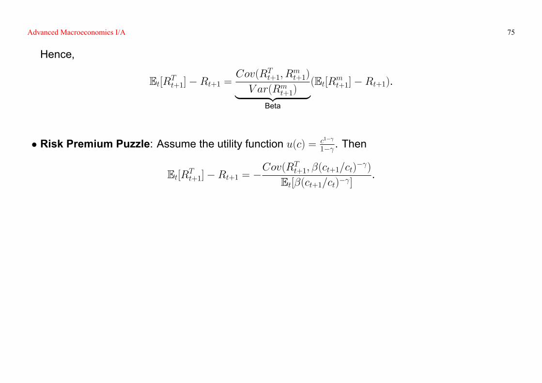
Hence,
Et[RTt+1]�Rt+1 =Cov(RTt+1; R
mt+1)
V ar(Rmt+1)| {z }Beta
(Et[Rmt+1]�Rt+1).
� Risk Premium Puzzle: Assume the utility function u(c) = c1�
1� . Then
Et[RTt+1]�Rt+1 = �Cov(RTt+1; �(ct+1=ct)
� )
Et[�(ct+1=ct)� ].
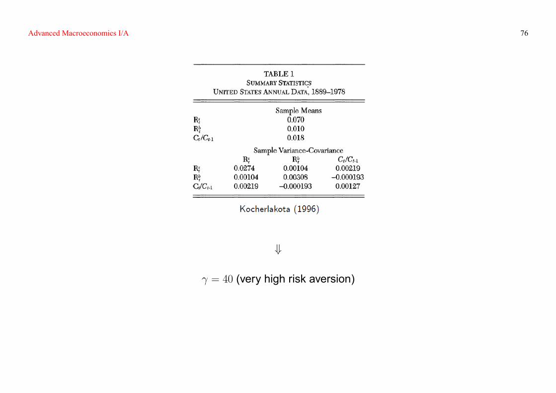
Advanced Macroeconomics I/A 76
+
= 40 (very high risk aversion)
Advanced Macroeconomics I/A 77
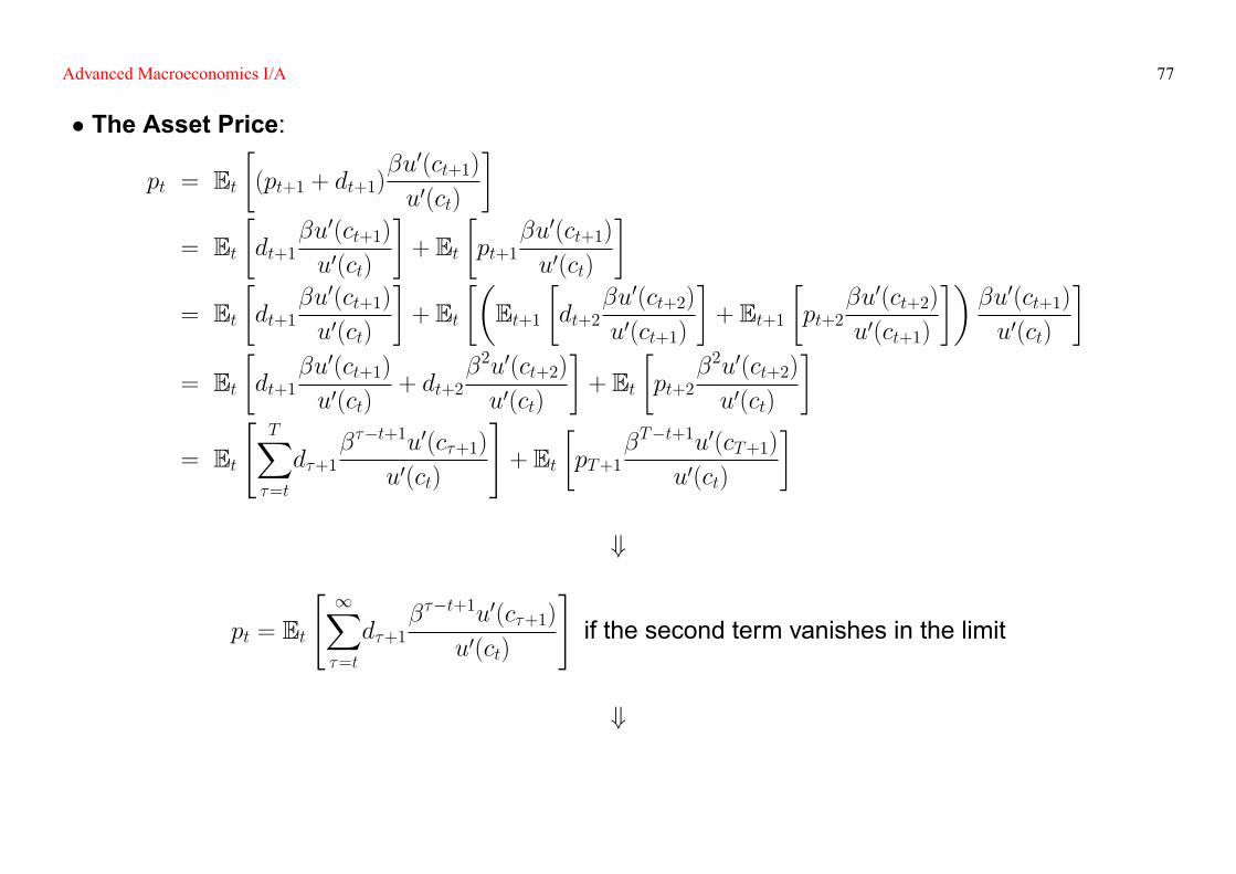
� The Asset Price:
pt = Et�(pt+1 + dt+1)
�u0(ct+1)
u0(ct)
�= Et
�dt+1
�u0(ct+1)
u0(ct)
�+ Et
�pt+1
�u0(ct+1)
u0(ct)
�= Et
�dt+1
�u0(ct+1)
u0(ct)
�+ Et
��Et+1
�dt+2
�u0(ct+2)
u0(ct+1)
�+ Et+1
�pt+2
�u0(ct+2)
u0(ct+1)
���u0(ct+1)
u0(ct)
�= Et
�dt+1
�u0(ct+1)
u0(ct)+ dt+2
�2u0(ct+2)
u0(ct)
�+ Et
�pt+2
�2u0(ct+2)
u0(ct)
�= Et
"TX�=t
d�+1���t+1u0(c�+1)
u0(ct)
#+ Et
�pT+1
�T�t+1u0(cT+1)
u0(ct)
�
+
pt = Et
" 1X�=t
d�+1���t+1u0(c�+1)
u0(ct)
#if the second term vanishes in the limit
+
Advanced Macroeconomics I/A 78
The Excess Volatility Puzzle: dividends should be more volatile than stock prices
� Bubbles: Consider an asset which doesn't pay any dividends. Assume �u0(ct+1)u0(ct)
= 1. Then
pt = Et[pt+1].
Question: Recursive Methods in Economic Dynamics, 3.3, 3.5;Question: Recursive Macroeconomic Theory, 2.1, 3.1;
5.12 References & Further Readings[1] Recursive Methods in Economic Dynamics, Chapter 2-4;[2] Recursive Macroeconomic Theory, Chapter 2-5.
Advanced Macroeconomics I/A 79
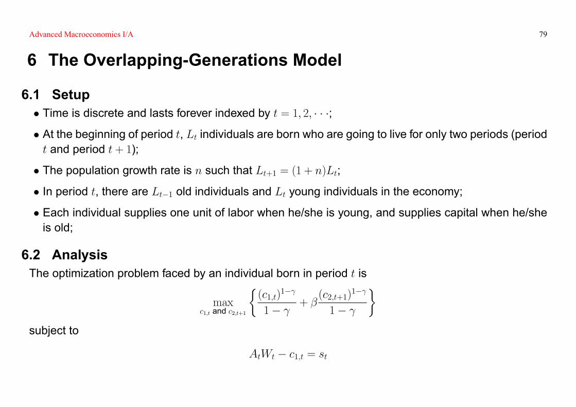
6 The Overlapping-Generations Model
6.1 Setup� Time is discrete and lasts forever indexed by t = 1; 2; � � �;
� At the beginning of period t, Lt individuals are born who are going to live for only two periods (periodt and period t + 1);
� The population growth rate is n such that Lt+1 = (1 + n)Lt;
� In period t, there are Lt�1 old individuals and Lt young individuals in the economy;
� Each individual supplies one unit of labor when he/she is young, and supplies capital when he/sheis old;
6.2 AnalysisThe optimization problem faced by an individual born in period t is
maxc1;t and c2;t+1
�(c1;t)
1�
1� + �(c2;t+1)
1�
1�
�subject to
AtWt � c1;t = st
Advanced Macroeconomics I/A 80
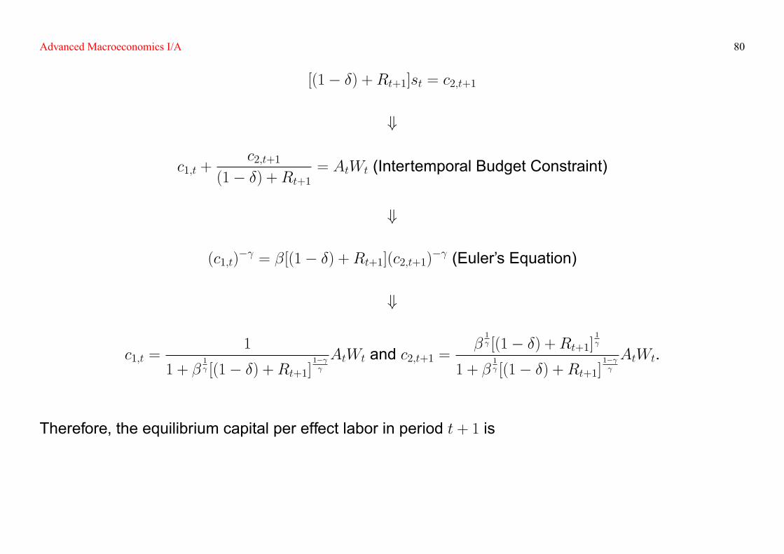
[(1� �) +Rt+1]st = c2;t+1
+
c1;t +c2;t+1
(1� �) +Rt+1= AtWt (Intertemporal Budget Constraint)
+
(c1;t)� = �[(1� �) +Rt+1](c2;t+1)� (Euler's Equation)
+
c1;t =1
1 + �1 [(1� �) +Rt+1]
1�
AtWt and c2;t+1 =�
1 [(1� �) +Rt+1]
1
1 + �1 [(1� �) +Rt+1]
1�
AtWt.
Therefore, the equilibrium capital per effect labor in period t + 1 is
Advanced Macroeconomics I/A 81
kt+1 =Ltst
At+1Lt+1=Lt(AtWt � c1;t)At+1Lt+1
=�
1 [(1� �) +Rt+1]
1�
(1 + g)(1 + n)n1 + �
1 [(1� �) +Rt+1]
1�
oWt
in which
Rt = f0(kt) andWt = f (kt)� f 0(kt)kt.
Assume = 1 and f (k) = k�. Then,
kt+1 =1
(1 + g)(1 + n)
�
1 + �(1� �)(kt)�
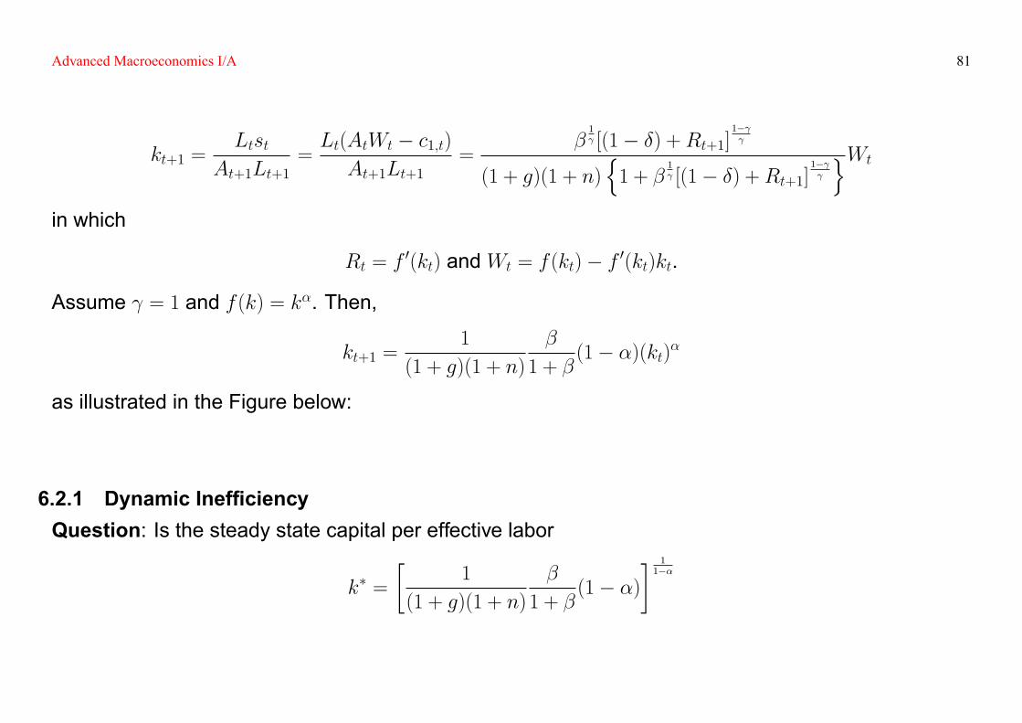
as illustrated in the Figure below:
6.2.1 Dynamic Inef�ciencyQuestion: Is the steady state capital per effective labor
k� =
�1
(1 + g)(1 + n)
�
1 + �(1� �)
� 11��
Advanced Macroeconomics I/A 82
less than the golden-rule capital per effective labor
kgold =
��
(1 + g)(1 + n)� (1� �)
� 11��
?
Answer: Not necessarily. For instance, if � is small enough.
6.2.2 Introduction of Government Expenditure� Denote gt as the government expenditure per effective labor in period t, which is �nanced by alump-sum labor income tax.
� The intertemporal budget constraint for an individual born in period t is
c1;t +c2;t+1
(1� �) +Rt+1= At(Wt � gt)
such that
kt+1 =1
(1 + g)(1 + n)
�
1 + �[(1� �)(kt)� � gt].
Question: What happens if there is an unexpected increase of government expenditure?
Answer: The steady state capital per effective labor decreases, which is not consistent with the pre-
Advanced Macroeconomics I/A 83
diction by the Ramsay model. Why?
6.2.3 How to Fix the Problem of Dynamic Inef�ciency?� No production;
� No storage technology available;
� Individuals are identical with y1 > 0 and y2 > 0;
� The utility function is
u(c1;t) + �u(c2;t+1).
� No trades between individuals in the same generation because individuals in the same generationsare identical;
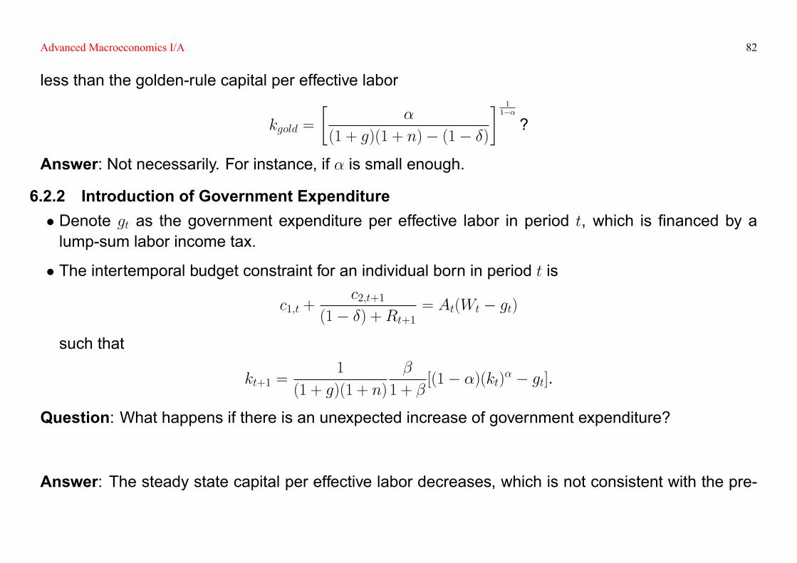
� No trades between individuals in different generations because (1) young individuals won't lend toold individuals. (2) old individuals won't lend to young individuals. Hence, the equilibrium is autarky:
c1;t = y1 and c2;t+1 = y2.
Solution 1: Consider the government's budget constraint in period t as
Lt� 1;t + Lt�1� 2;t � 0
where � 1;t is the lump-sum tax on the young generation, and � 2;t is the lump-sum tax on the old
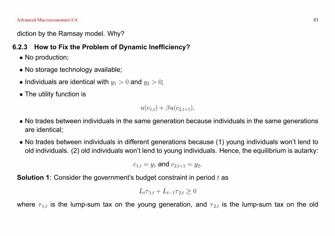
Advanced Macroeconomics I/A 84
generation in period t as illustrated in the Figure below:
tc ,2
tc ,1
2y
1y*1c
*2c
Solution 2: Fiat Money� The money supply is �xed atM s > 0.
� The optimization problem faced by an individual born in period t is
maxc1;t and c2;t+1
u(c1;t) + �u(c2;t+1)
Advanced Macroeconomics I/A 85
subject to
Pt(y1 � c1;t) =Mdt
Pt+1(c2;t+1 � y2) =Mdt .
+
u0(c1;t) = �PtPt+1
u0(c2;t+1) (Euler's Equation)
+
Mdt
Pt=M
�PtPt+1
; y1; y2
�� 0 (Money Demand Function)
Furthermore, the money market clearing condition is
LtM
�PtPt+1
; y1; y2
�=M s
Pt, for t = 1; 2; � � �
Advanced Macroeconomics I/A 86
which implies that in the steady state
LtM�PtPt+1; y1; y2
�Lt+1M
�Pt+1Pt+2; y1; y2
� = Pt+1Pt
+
PtPt+1
= 1 + n, for t = 1; 2; � � �
Question: Is money neutral in this economy?Answer: Yes.
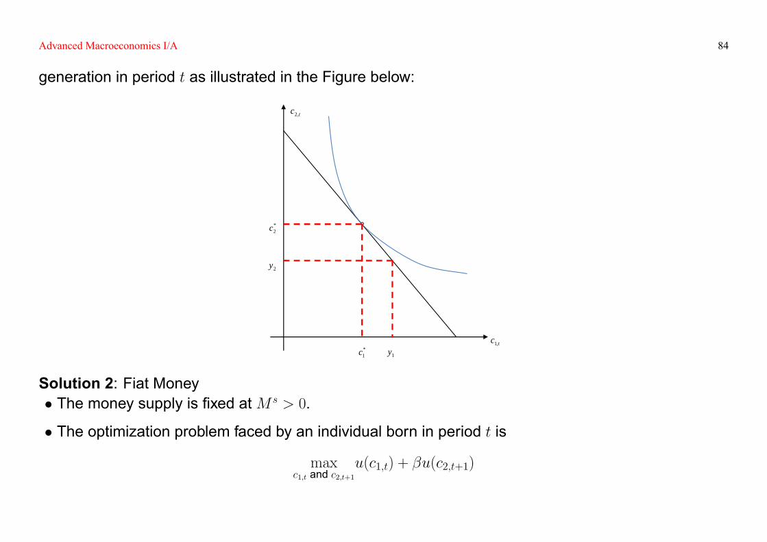
Question: What happens if a storage technology with the gross return rate 1 + r is introduced?Answer: Whether money will be valued in the equilibrium depends on r > n, or r < n as illustrated in
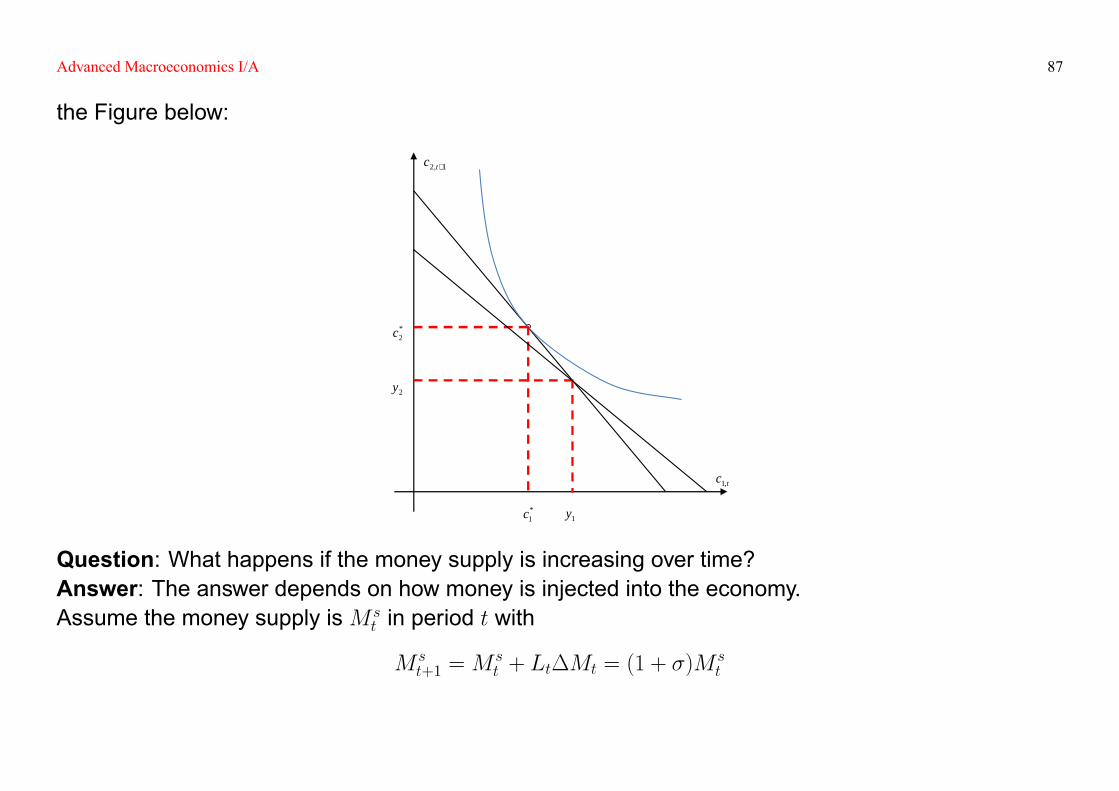
Advanced Macroeconomics I/A 87
the Figure below:
1,2 +tc
tc ,1
2y
1y*1c
*2c
Question: What happens if the money supply is increasing over time?Answer: The answer depends on how money is injected into the economy.Assume the money supply isM s
t in period t with
M st+1 =M
st + Lt�Mt = (1 + �)M
st
Advanced Macroeconomics I/A 88
where �Mt is the lump sum money transfer the old individuals in period t + 1.Thus, the optimization problem faced by an individual born in period t is
maxc1;t and c2;t+1
u(c1;t) + �u(c2;t+1)
subject to
Pt(y1 � c1;t) =Mdt
Pt+1(c2;t+1 � y2) =Mdt +�Mt.
+
Mdt
Pt=M
�PtPt+1
;�Mt
Pt+1; y1; y2
�Furthermore, the money market clearing condition is
LtM
�PtPt+1
;�Mt
Pt+1; y1; y2
�=M st
Pt, for t = 1; 2; � � �
Advanced Macroeconomics I/A 89
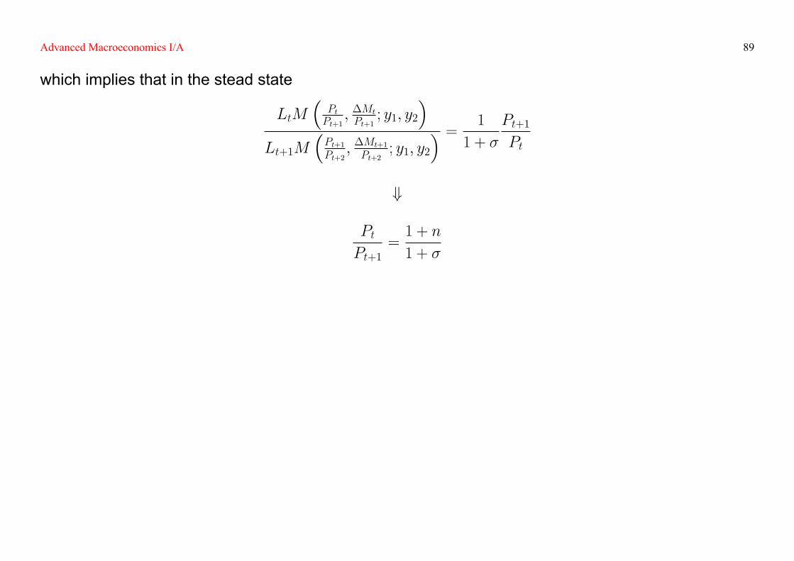
which implies that in the stead state
LtM�PtPt+1; �Mt
Pt+1; y1; y2
�Lt+1M
�Pt+1Pt+2; �Mt+1
Pt+2; y1; y2
� = 1
1 + �
Pt+1Pt
+
PtPt+1
=1 + n
1 + �
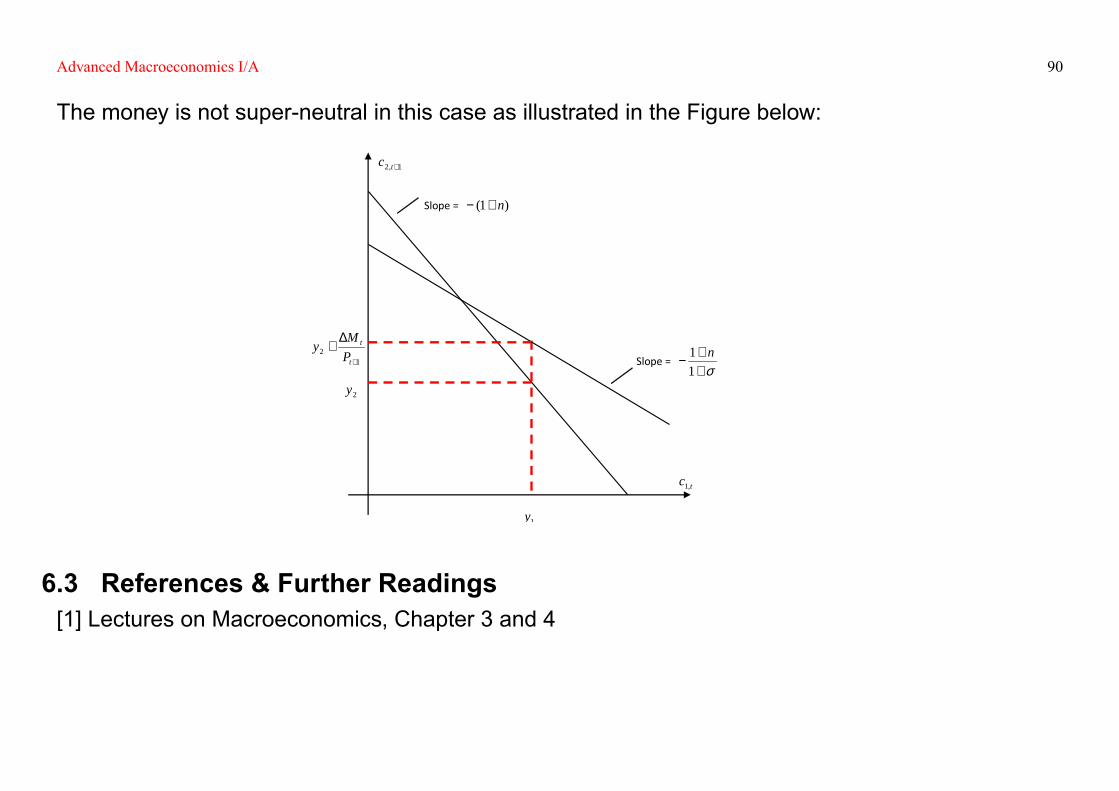
Advanced Macroeconomics I/A 90
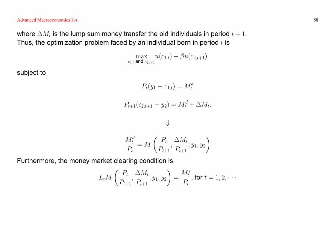
The money is not super-neutral in this case as illustrated in the Figure below:
1,2 +tc
tc ,1
2y
1y
12
+
∆+
t
t
PM
y
Slope = )1( n+−
Slope =σ+
+−
11 n
6.3 References & Further Readings[1] Lectures on Macroeconomics, Chapter 3 and 4
Advanced Macroeconomics I/A 91
7 The Real Business Cycle Model
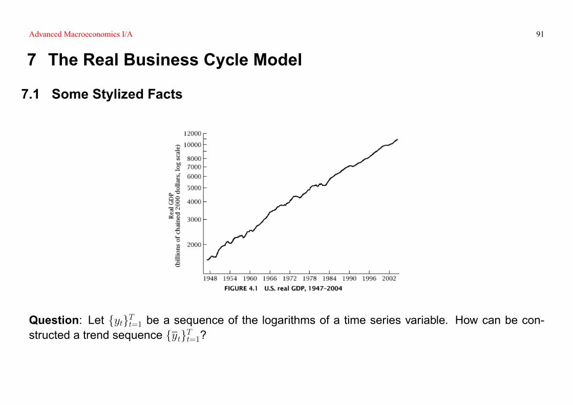
7.1 Some Stylized Facts
Question: Let fytgTt=1 be a sequence of the logarithms of a time series variable. How can be con-structed a trend sequence fytgTt=1?
Advanced Macroeconomics I/A 92
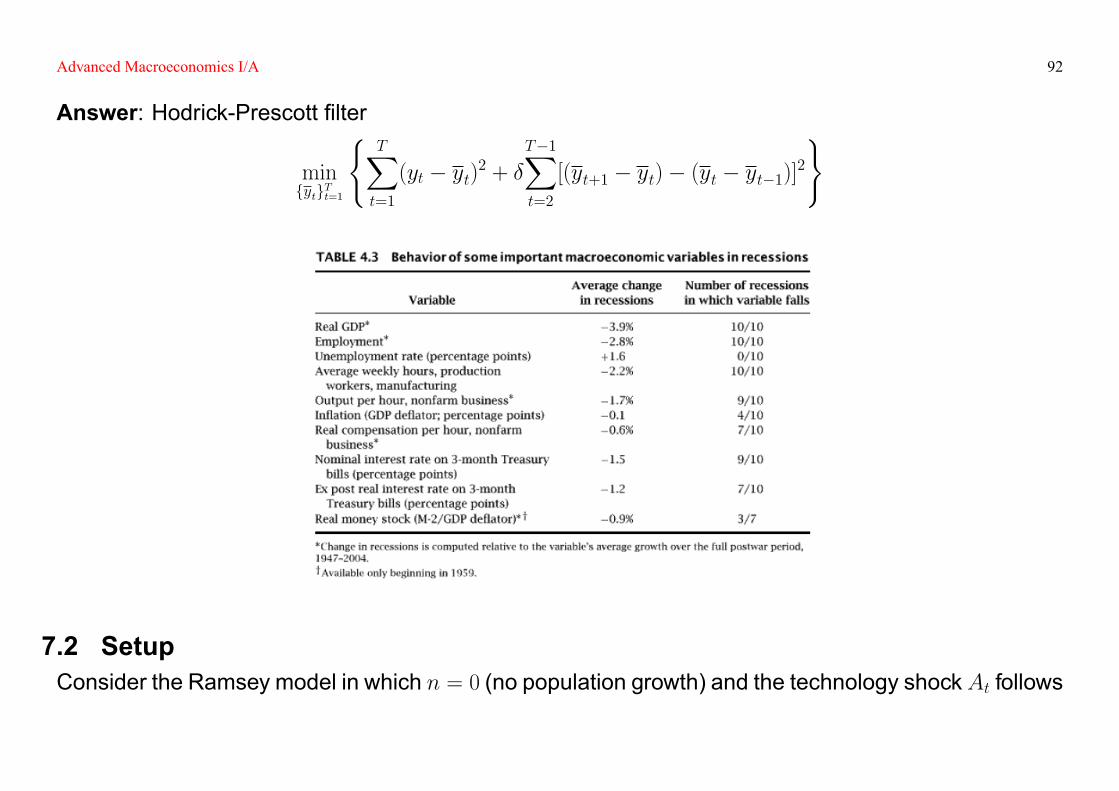
Answer: Hodrick-Prescott �lter
minfytgTt=1
(TXt=1
(yt � yt)2 + �T�1Xt=2
[(yt+1 � yt)� (yt � yt�1)]2)
7.2 SetupConsider the Ramsey model in which n = 0 (no population growth) and the technology shockAt follows
Advanced Macroeconomics I/A 93
an AR(1) process with a trend.
7.3 AnalysisGiven K0 > 0, the representative household's optimization problem is
maxfKt+1;Ctg1t=0
(E0
" 1Xt=0
�tu(Ct)
#)subject to
Kt+1 = K�t A
1��t + (1� �)Kt � Ct for t = 0; 1; � � � (21)
At follows an AR(1) process with a trend
Let f�t Pr(At)�t(At)g1t=0 be the Lagrangian multipliers. Then the �rst order conditions are
�t = �Et
"�t+1
�
�Kt+1At+1
���1+ (1� �)
!#
u0(Ct) = �t
+
Advanced Macroeconomics I/A 94
1 = �Et
"�Ct+1Ct
�� �
�Kt+1At+1
���1+ (1� �)
!#(Euler's Equation)
Step 1 The Steady State
1 = �Et
"�(1 + g)
Ct+1=At+1Ct=At
�� �
�Kt+1At+1
���1+ (1� �)
!#(22)
(1 + g)Kt+1At+1
=
�KtAt
��+ (1� �)Kt
At� CtAt
(23)
+
1 = �(1 + g)� [�(k�)��1 + (1� �)]
(1 + g)k� = (k�)� + (1� �)k� � c�
Step 2 Log-LinearizationFor instance, it takes three steps to log-linearizing (21) as follows:
Advanced Macroeconomics I/A 95
(i) Denote Kt = lnKt, Ct = lnCt, and At = lnAt. Then rewrite (21) as
exp(Kt+1) = (exp(Kt))�(exp(At))
1�� + (1� �) exp(Kt)� exp(Ct)
(ii) Take the �rst order Taylor expansion at (Kt = lnK�t ; Ct = lnC
�t ; At = lnA
�t ) as
K�t+1(Kt+1 � lnK�
t+1) = �
�K�t
A�t
���1K�t (Kt � lnK�
t ) + (1� �)�K�t
A�t
��A�t (At � lnA�t )
+(1� �)K�t (Kt � lnK�
t )� C�t (Ct � lnC�t )
(iii) Denote bKt = lnKt � lnK�t , bCt = lnCt � lnC�t , and bAt = lnAt � lnA�t . Then
(1 + g) bKt+1 = [�(k�)��1 + (1� �)] bKt � c�
k�bCt + (1� �)(k�)��1 bAt (24)
Similarly, we can log-linearize the Euler's equation as well.Step 3 KPR Method
Advanced Macroeconomics I/A 96
For instance, suppose Et[ bAt+1] = � bAt. Then we have three linear equations as follows264 bKt+1Et[ bCt+1]Et[ bAt+1]
375 = W264 bKtbCtbAt
375 (25)
(i) Given the eigenvalue decomposition ofW as
W = P
24 '1 0 0
0 '2 0
0 0 '3
35P�1where '1; '2; '3 are the eigenvalues ofW , rewrite (25) as264 bKt
E0[ bCt]E0[ bAt]
375 = P24 't1 0 0
0 't2 0
0 0 't3
35P�1264 bK0bC0bA0
375 .(ii) One of the eigenvalues of W is greater than one. Without loss of generality, let '1 > 1. Therefore,

Advanced Macroeconomics I/A 97
in order to avoid the explosive path, we must have
P�1
264 bK0bC0bA0375 =
24 0bd
35+264 bK0bC0bA0
375 = P24 0bd
35+264 bK0bC0bA0
375 = P [�; (2; 3)] � bd
�
+
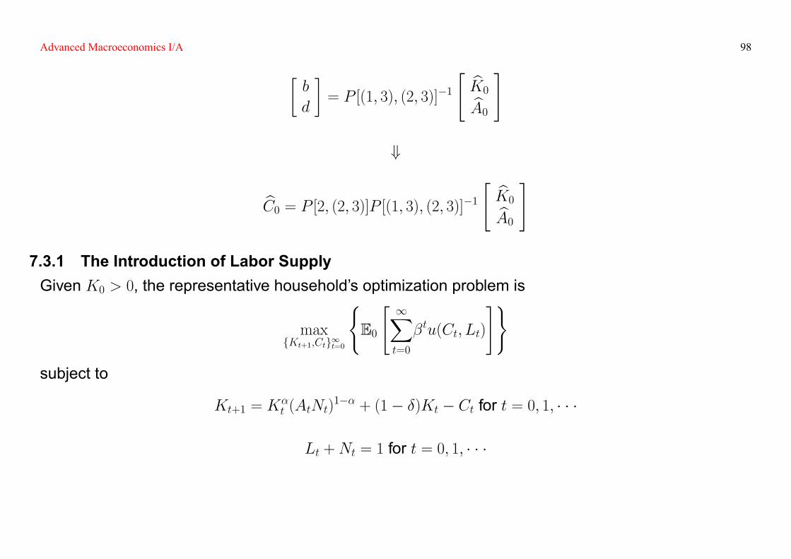
Advanced Macroeconomics I/A 98�b
d
�= P [(1; 3); (2; 3)]�1
" bK0bA0#
+
bC0 = P [2; (2; 3)]P [(1; 3); (2; 3)]�1 " bK0bA0#
7.3.1 The Introduction of Labor SupplyGiven K0 > 0, the representative household's optimization problem is
maxfKt+1;Ctg1t=0
(E0
" 1Xt=0
�tu(Ct; Lt)
#)subject to
Kt+1 = K�t (AtNt)
1�� + (1� �)Kt � Ct for t = 0; 1; � � �
Lt +Nt = 1 for t = 0; 1; � � �
Advanced Macroeconomics I/A 99
At follows an AR(1) process with a trend
Question: What assumptions do we have to make about the utility function in order to have a steadystate?Answer: For instance,
u(Ct; Lt) =C1� t
1� v(Lt).
7.4 References & Further Readings[1] Advanced Macroeconomics, Chapter 4[2] King, R. G., C. I. Plosser, and S. T. Rebelo (1988): Production, Growth and Business Cycles I. TheBasic Neoclassical Model, Journal of Monetary Economics, 21(2), 195-232.