Embed Size (px)
Citation preview

Advanced Micro Theory
Preferences and Utility
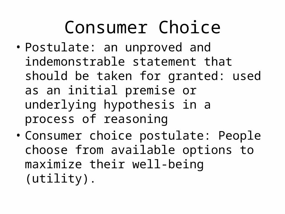
Consumer Choice• Postulate: an unproved and indemonstrable
statement that should be taken for granted: used as an initial premise or underlying hypothesis in a process of reasoning
• Consumer choice postulate: People choose from available options to maximize their well-being (utility).
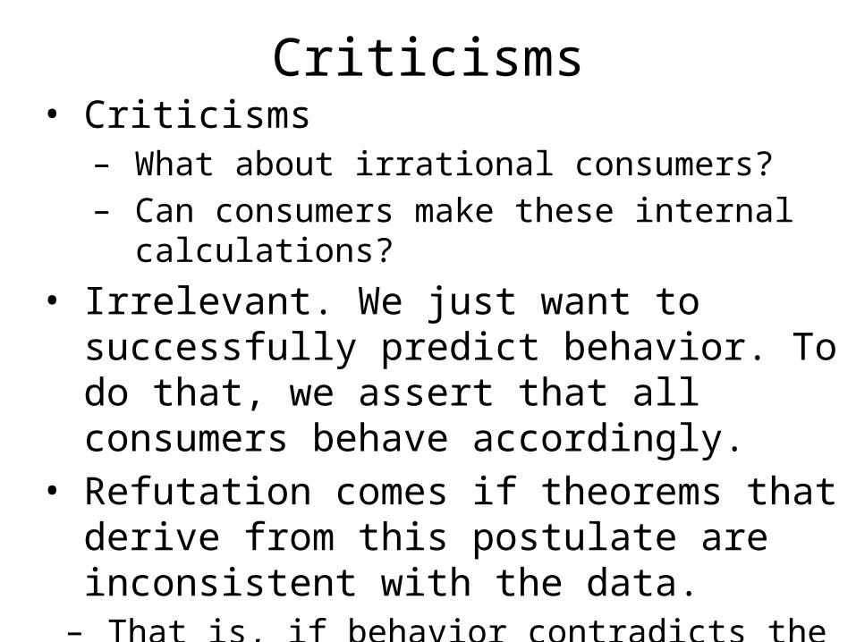
Criticisms• Criticisms
– What about irrational consumers?– Can consumers make these internal calculations?
• Irrelevant. We just want to successfully predict behavior. To do that, we assert that all consumers behave accordingly.
• Refutation comes if theorems that derive from this postulate are inconsistent with the data.
– That is, if behavior contradicts the implications of the model, then the theory is wrong.
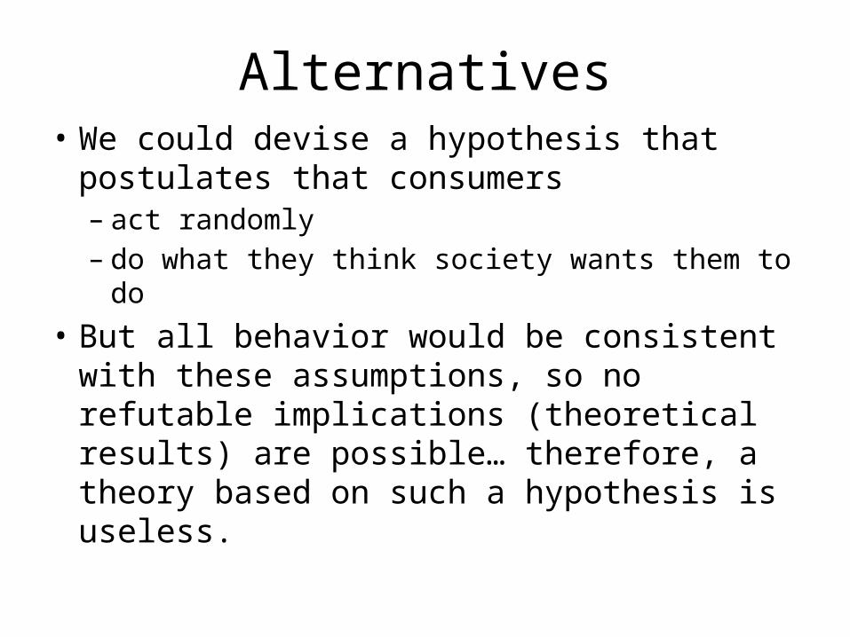
Alternatives• We could devise a hypothesis that postulates
that consumers– act randomly– do what they think society wants them to do
• But all behavior would be consistent with these assumptions, so no refutable implications (theoretical results) are possible… therefore, a theory based on such a hypothesis is useless.

Consumer Choice Model• “People choose from available options to
maximize their well-being (utility).”– “Available options” in the model will be handled by
the budget constraint.• The budget constraint will provide decision-makers with
MC of choices.
– “Maximizing well-being” will be incorporated into the model via assumptions about preferences – which will then be used to build a utility function.
• The preferences part of the model will provide decision-makers with the MB of choices.
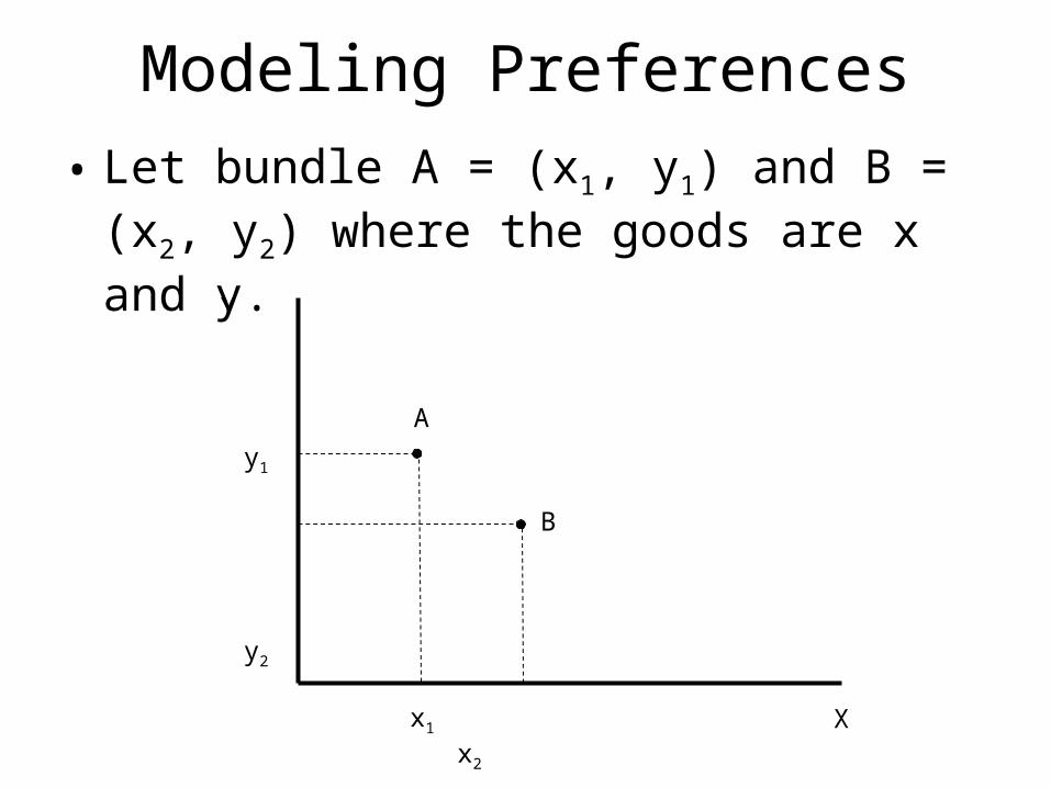
Modeling Preferences• Let bundle A = (x1, y1) and B = (x2, y2) where
the goods are x and y.Y
X
A
B
x1 x2
y1
y2
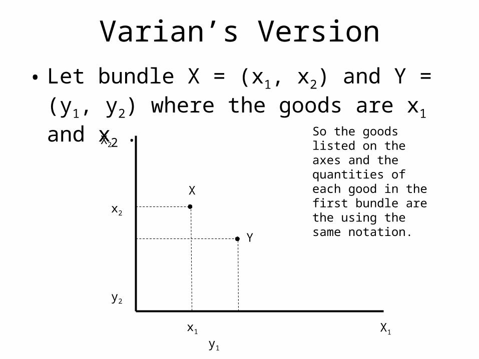
Varian’s Version• Let bundle X = (x1, x2) and Y = (y1, y2) where the
goods are x1 and x2 . X2
X1
X
Y
x1 y1
x2
y2
So the goods listed on the axes and the quantities of each good in the first bundle are the using the same notation.
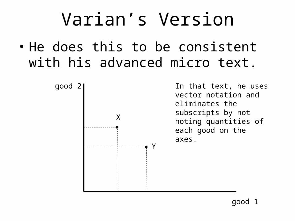
Varian’s Version• He does this to be consistent with his
advanced micro text.
good 2
good 1
X
Y
In that text, he uses vector notation and eliminates the subscripts by not noting quantities of each good on the axes.

Modeling Preferences• IMO, students have invested so much math time with X and Y on the axes,
that I want to leverage that. E.g. slope = • Also, with all the derivations coming up, we will have plenty of subscripts
floating around that I hate to add an additional set with goods X1 and X2.
Y
X
A
B
x1 x2
y1
y2
dy
dx

Modeling Preferences• Three choices:
• And thereforeY
X
A
B
x1 x2
y1
y2
A B, consumer strictly prefers bundle A to bundle B
A B, consumer weakly prefers bundle A to bundle B
A B, consumer indifferent between bundle A and bundle B
If A B, and B A then A B
If A B, and not A B then A B

Axioms of Preference• Axiom: a proposition that is assumed without proof for
the sake of studying the consequences that follow from it (dictionary.com). – These are based on ensuring logical consistency.
• Completeness: – Any pair of bundles can be compared and ordered
• Reflexivity: – A bundle cannot be strictly preferred to an identical bundle.
• Transitivity
– Not a logical imperative according to Varian, but preferences become intractable if people cannot choose between three bundles because
• Continuity, next page
3 3Let C = (x ,y )
If A B, and B C then A C
A B, or B A, or both, meaning A B.
A A , or A A
A B, and B C and C A
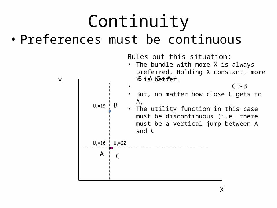
Continuity• Preferences must be continuous
Y
X
A
B
C
Rules out this situation:• The bundle with more X is always preferred. Holding
X constant, more Y is better.• • But, no matter how close C gets to A, • The utility function in this case must be
discontinuous (i.e. there must be a vertical jump between A and CUb=15
Uc=20Ua=10
B A, C A C B

Goods, Bads and Neutral Goods
• Goods are good (more is better)• Bads are bad, less is better• Neutrals mean nothing to the consumer• Some goods start out good, but then become
bads if you consume too much

Possible Indifference Mappings Thus FarCharacterize the Goods
X
Y
X
Y
X
Y
X
Y
X
Y
X
Y
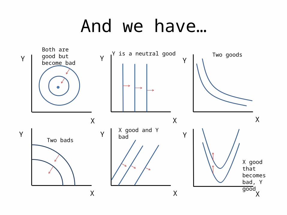
And we have…
X
Y
X
Y
X
Y
X
Y
X
Y
X
YTwo goodsY is a neutral good
Both are good but become bad
Two bads
X good and Y bad
X good that becomes bad, Y good
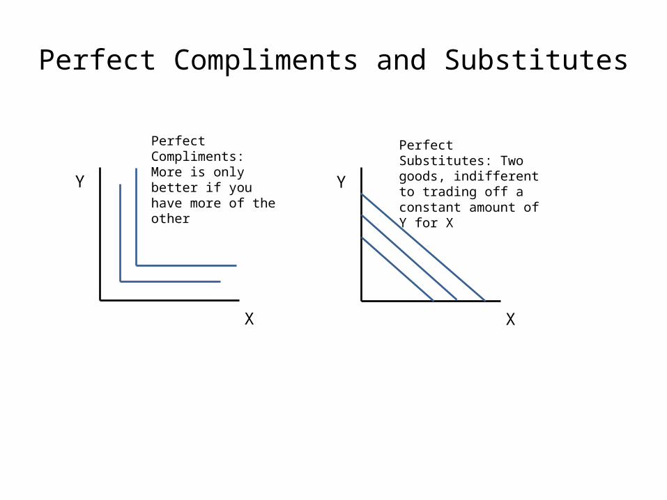
Perfect Compliments and Substitutes
X
Y
X
Y
Perfect Compliments: More is only better if you have more of the other
Perfect Substitutes: Two goods, indifferent to trading off a constant amount of Y for X
Well-behaved Preferences• If we want to avoid situations where demand
curves are upward sloping or people spend all their money on one good, then we need well-behaved indifference curves.
• Preferences must also be – Monotonic– Convex

Monotonic• Monotonic: If bundle A is identical to B, except
A has more of at lease one good, then– A.K.A, nonsatiation or “more-is-better”– Ceteris paribus, increasing the quantity of one
good creates a bundle that is strictly preferred.– Indifference curves must be downward sloping.– Paired with transitivity, means indifference curves
cannot cross.
A B
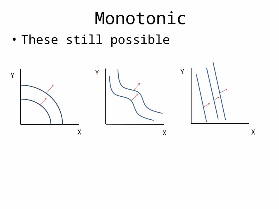
Monotonic• These still possible
X
Y
X
Y
X
Y

Indifference Curves Cannot Cross
X
Y A
B
C
A C, share an indifference curve
B C, share an indifference curve
A B, transitivity
But A B, monotonicity
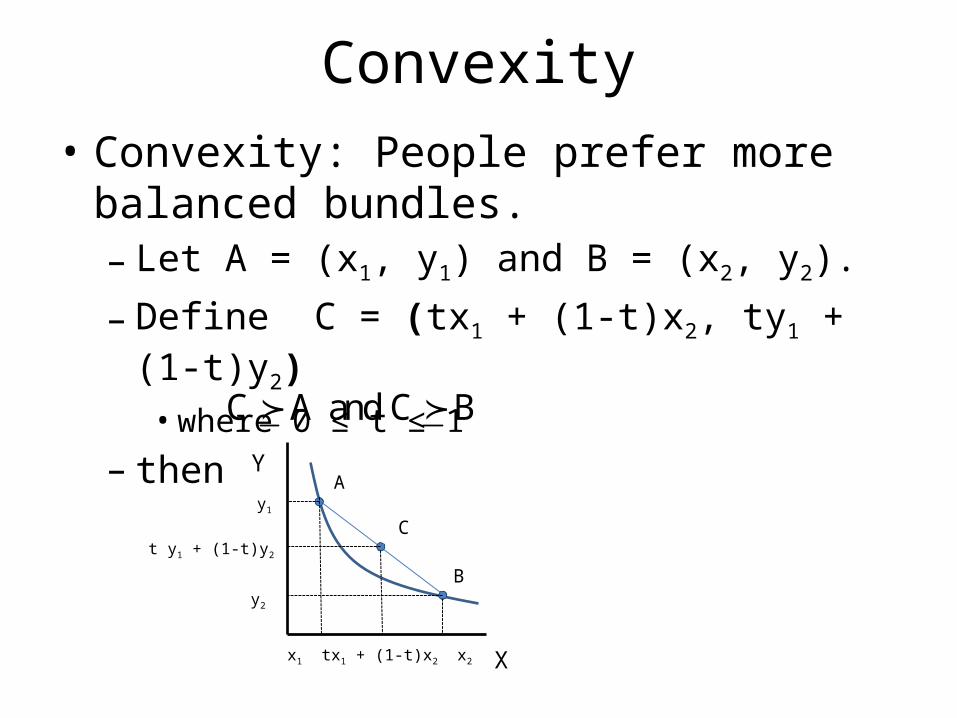
Convexity• Convexity: People prefer more balanced
bundles.– Let A = (x1, y1) and B = (x2, y2).
– Define C = (tx1 + (1-t)x2, ty1 + (1-t)y2)• where 0 ≤ t ≤ 1
– then C A and C B
X
YA
B
C
x1 tx1 + (1-t)x2 x2
y1
t y1 + (1-t)y2
y2
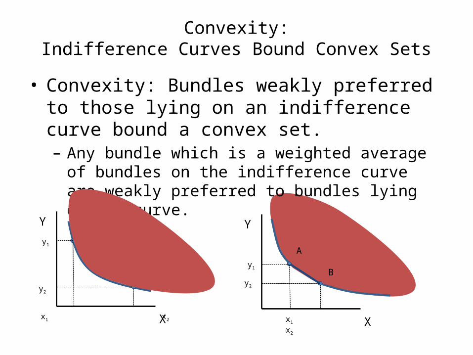
Convexity:Indifference Curves Bound Convex Sets
• Convexity: Bundles weakly preferred to those lying on an indifference curve bound a convex set.– Any bundle which is a weighted average of bundles on the
indifference curve are weakly preferred to bundles lying on the curve.
X
YA
B
x1 x2
y1
y2
X
Y
A
B
x1 x2
y1
y2
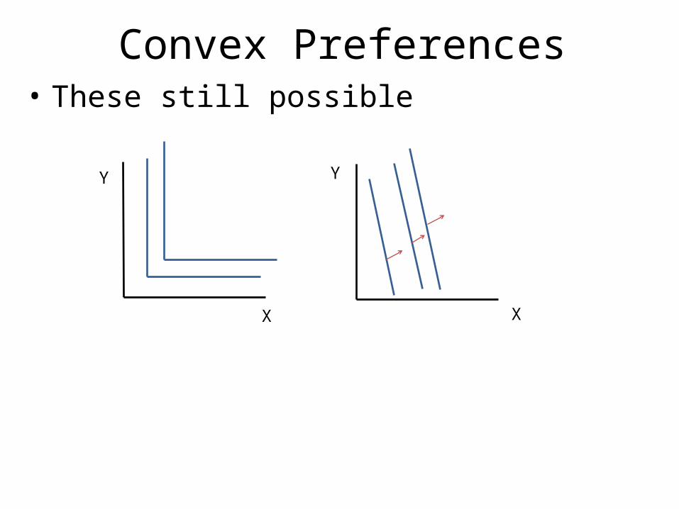
Convex Preferences• These still possible
X
Y
X
Y

Strict ConvexityIndifference Curves Bound Convex Sets
• Strictly Convex Preferences: – Any bundle which is a weighted average of bundles on the
indifference curve are strictly preferred to bundles lying on the curve (weights 0 > t > 1).
– Simple convexity allows for straight line segments of the indifference curve
– Strict convexity does not, the curve must have an increasing slope as X increases.
X
YA
B
y1
y2
x1 tx1 + (1-t)x2 x2
ty1 + (1-t)y2 C
C A, C B

Convexity• Intuition: people prefer balanced bundles of
goods to bundles with a lot of one good and little of the other good.
Y
X
U=4
U=7
U=10
U=7
U=4
Along a straight lineconnecting the axis,Utilty will rise and thenfall.
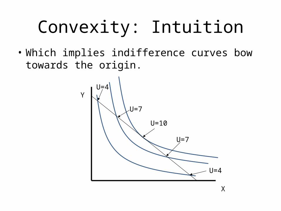
Convexity: Intuition• Which implies indifference curves bow towards the
origin.
Y
X
U=4
U=7
U=10
U=7
U=4

Marginal Rate of Substitution• The change in the consumption of the good on
the Y axis necessary to maintain utility if the consumer increases consumption of the good on the X axis by one unit.
• MRS = the slope of the indifference curve.
• Although, , MRS is almost always defined as the abs value of the slope.
• In this class, dyMRS
dx
dy0
dx

MRS = MB
• The MRS describes, at any given point along the indifference curve, the consumer’s willingness to give up Y for one more X.
• It is therefore the marginal willingness to pay for X
• I.e. it is the marginal benefit of consuming X.

Digression: Cardinal Utility• Utilitarians believed that utility, like temperature or height, was
something that was measurable (Cardinal utility).– And that a unit of utility was the same for everyone so if we could find out
how to measure it, we could redistribute to maximize social welfare.– The hope of some way of measuring utils did not survive long.
• Early neoclassical economists (e.g. Marshall) still held the idea that for an individual, utility may be a cardinal measure.– Believed marginal utility was strictly decreasing.– Marshall’s demand curve was downward sloping for this reason.– He is the reason P is on the vertical axis. Diminishing willingness to pay
reflected diminishing marginal utility.• Also believed that utility was additive, consumption of one good
did not affect the MU from another (Uxy = 0).

Digression: Ordinal Utility• Pareto (1906) first considered the idea that ordinal
utility (ordering the desirability of different choices) might be the way to think of utility.
• Work by Edgeworth, Fischer and Slutsky advanced the theory.
• Hicks and Allen (1934) came up with the defining theory… that we still use today.
• Pareto, Vilfredo (1906). "Manuale di economia politics, con una introduzione ulla scienza sociale". Societa Editrice Libraria.
• Viner, Jacob. (1925a). "The utility concept in value theory and its critics". Journal of political economy Vol. 33, No. 4, pp. 369-387
• Hicks, John and Roy Allen. (1934). "A reconsideration of the theory of value". Economica Vol. 1, No. 1, pp. 52-76
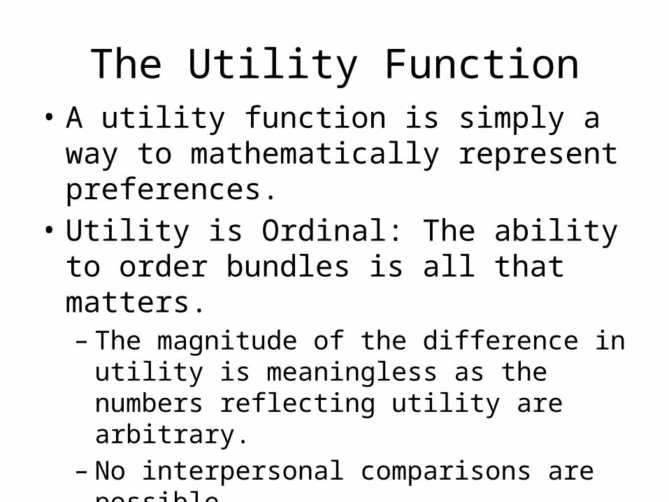
The Utility Function• A utility function is simply a way to
mathematically represent preferences.• Utility is Ordinal: The ability to order bundles
is all that matters.– The magnitude of the difference in utility is
meaningless as the numbers reflecting utility are arbitrary.
– No interpersonal comparisons are possible.

The Utility Function• A function such that
• Preference can be represented by a continuous U=U(A) so long as preferences are reflexive, complete, transitive, continuous
• Note, monotonacity and convexity are not needed.
• Monotonacity is always assumed because it makes the existence proof easier and more intuitive.
A B if and only if U(A) U(B)

The Utility Function• While we need preferences to be reflexive,
complete, transitive, continuous for utility functions to exist.
• We need monotonacity and convexity to make them well behaved.
• By well behaved, we want unique solutions that are not extreme and are relatively stable.– We don’t want individuals spending all their
income on one good or slight changes in price or income to drastically affect the optimal choice.

Revisiting Monotonacity• As all indifference curves are strictly
downward sloping, they will all cross a 45 deg line.
x
y d
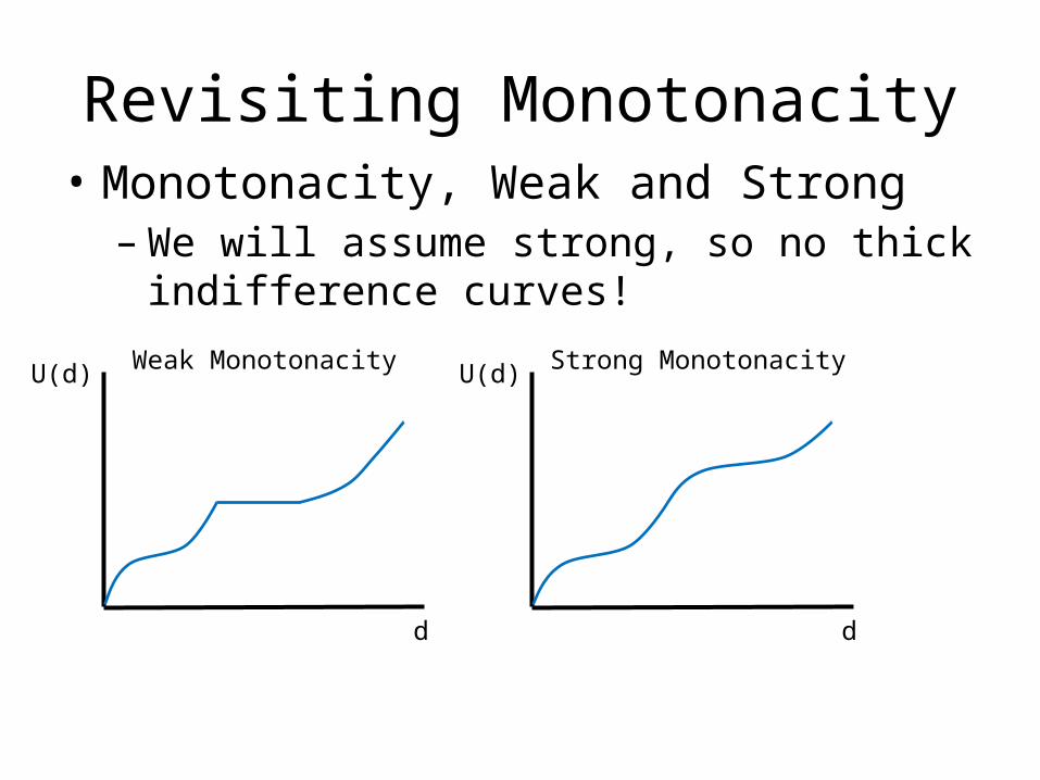
Revisiting Monotonacity• Monotonacity, Weak and Strong
– We will assume strong, so no thick indifference curves!
U(d)
d
Weak Monotonacity U(d)
d
Strong Monotonacity
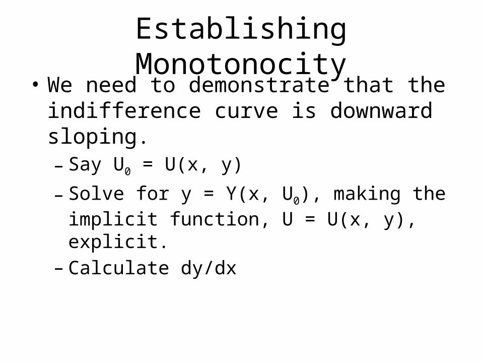
Establishing Monotonocity• We need to demonstrate that the indifference
curve is downward sloping.– Say U0 = U(x, y)
– Solve for y = Y(x, U0), making the implicit function, U = U(x, y), explicit.
– Calculate dy/dx
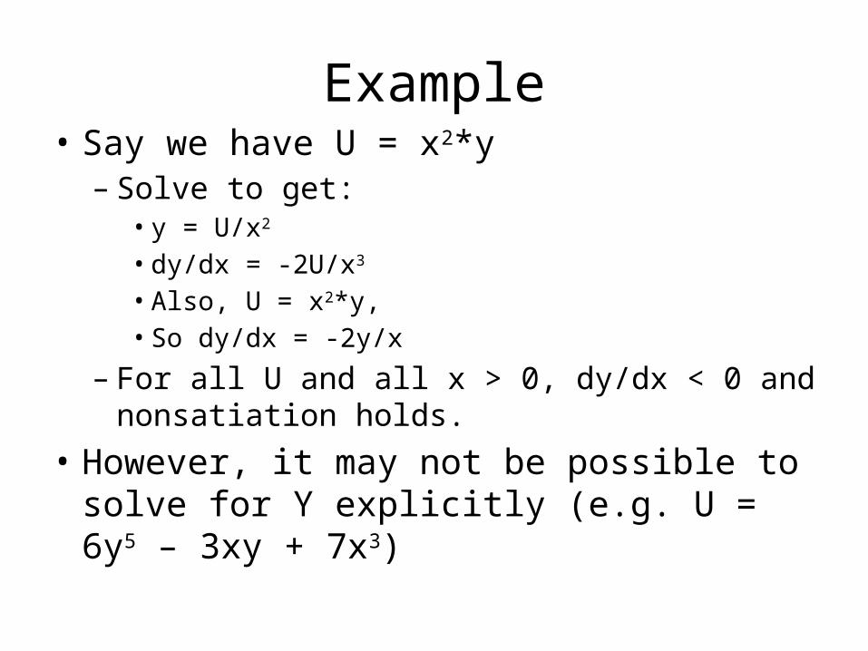
Example• Say we have U = x2*y
– Solve to get:• y = U/x2 • dy/dx = -2U/x3 • Also, U = x2*y, • So dy/dx = -2y/x
– For all U and all x > 0, dy/dx < 0 and nonsatiation holds.
• However, it may not be possible to solve for Y explicitly (e.g. U = 6y5 – 3xy + 7x3)

dy/dx via Implicit Differentiation• We start with an implicit function (identity) defining an
indifference curve. To hold when x changes, y must change too.
0
0
0
x x
y y
U U x, y(x)
dU x, y(x)dU
dx dxU x, y(x) U x, y(x)dU dx dy
dx x dx y dx
U x, y(x) U x, y(x) dy0
x y dx
U x, y(x) U x, y(x)dy
y dx x
U x, y(x)U (x, y) Udy x
U x, y(x)dx U (x, y) U
y
https://www.khanacademy.org/math/calculus/differential-calculus/implicit_differentiation/v/implicit-differentiation-1
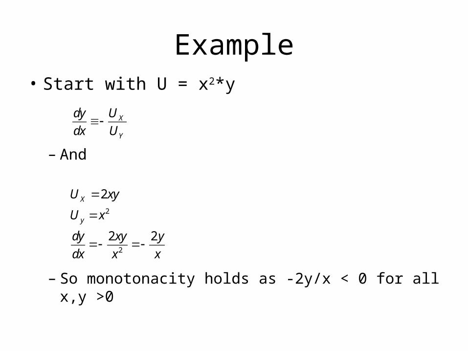
Example• Start with U = x2*y
– And
– So monotonacity holds as -2y/x < 0 for all x,y >0
X
Y
Udy
dx U
2
2
2
2 2
X
y
U xy
U x
dy xy y
dx x x
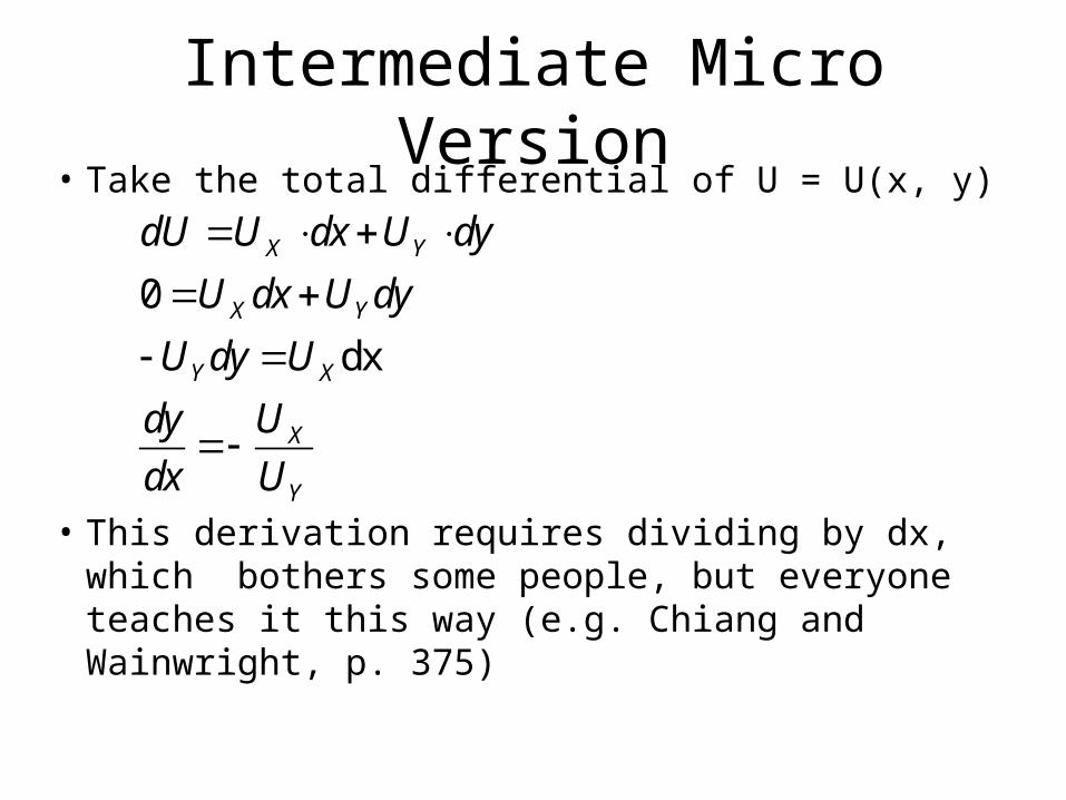
Intermediate Micro Version• Take the total differential of U = U(x, y)
• This derivation requires dividing by dx, which bothers some people, but everyone teaches it this way (e.g. Chiang and Wainwright, p. 375)
0
dx
X Y
X Y
Y X
X
Y
dU U dx U dy
U dx U dy
U dy U
Udy
dx U
Transformations• It sometimes makes life computationally easier to
transform a utility function.• Start with utility function that is well behaved
(satisfies all the axioms of preference).• We can transform that function with no loss of
information so long as the relationship between any bundles A and B is unchanged.

Positive Monotonic Transformations
• Two functions with identical ordinal properties are called Positive Monotonic Transformations of one another.
• Both functions will create identically SHAPED indifference curves (although the utility value associated with each curve will differ).
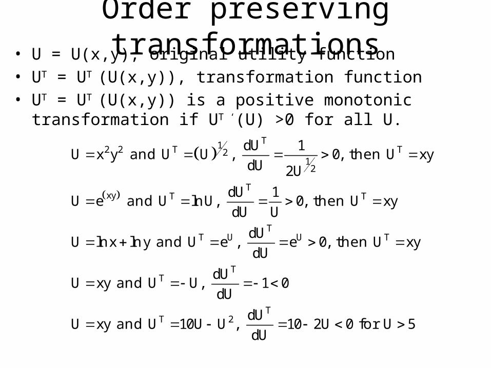
Order preserving transformations• U = U(x,y), original utility function• UT = UT (U(x,y)), transformation function • UT = UT (U(x,y)) is a positive monotonic transformation if UT ‘(U) >0
for all U.
T12 2 T T21
2
Txy T T
TT U U T
TT
TT 2
dU 1U x y U U 0 U xy
dU 2U
dU 1U e U ln U 0 U xy
dU U
dUU ln x ln y U e e 0 U xy
dU
dUU xy U U 1 0
dU
dUU xy U 10U U 10 2U 0 U 5
dU
and , , then
and , , then
and , , then
and ,
and , for

Convexity• That is, MRS diminishes as x increase and y
decreases. It is about curvature.This Not this
MRS = 5
MRS = 2
MRS = 1
X
Y
X
Y MRS = 5
MRS = 5
MRS = 2
MRS = 2
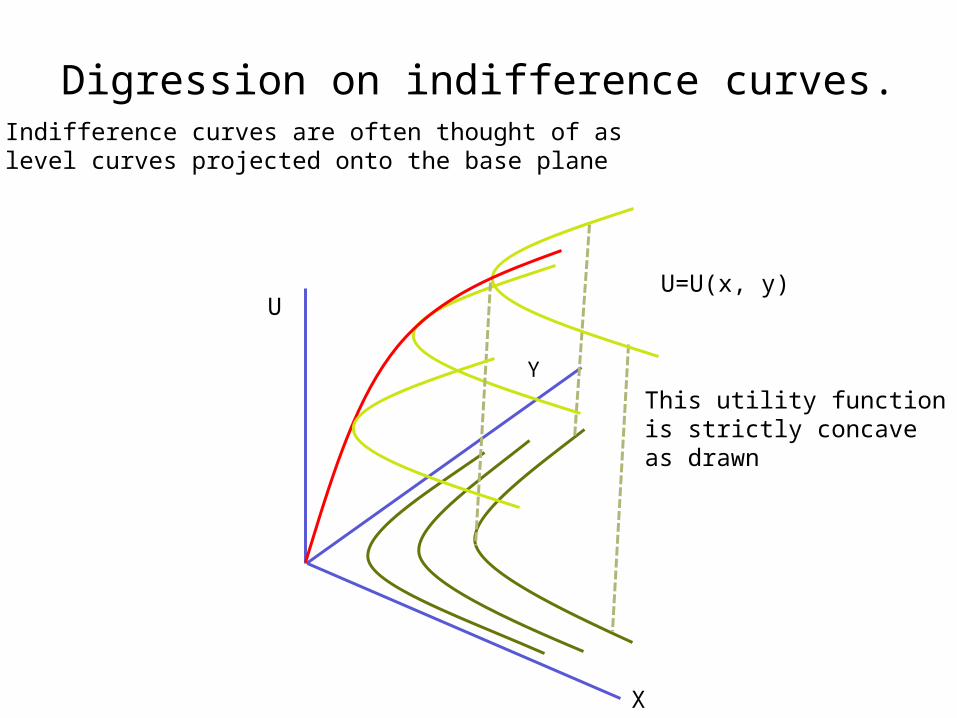
Digression on indifference curves.Indifference curves are often thought of as level curves projected onto the base plane
This utility functionis strictly concaveas drawn
Y
U=U(x, y)
X
U
Indifference Curves are Level Curves
• Level Curves– Are a slice of the utility function at some U = U0 – Even if the utility function is not concave (as drawn
above), but only strictly quasi concave, these level curves bound convex sets
– Convex sets and level curves• Any line connecting two points on the same level curve lies
within the set• So bundles with more balance than two bundles lying on an
indifference curve will provide more utility (the utility function will be “above” any line connecting two points on an indifference curve.

Convexity• Convexity
– DOES NOT IN ANY WAY indicate that the utility function is convex as opposed to concave.
– Convex functions and convex sets are two different concepts.
• “Strictly”– Strictly quasi–concave utility function means the
utility function has no flat spots and it’s level sets are strictly convex
– Strictly convex level curves means the indifference curves have no straight line segments
– “Strictly” required to ensure just one optimum

Convexity of Preferences Implies Indifference Curves Bound Convex SetsThis will hold if the utility function is Strictly Quasi Concave
Utility Function Not Concave, but Strictly Quasi Concave as the level sets bound convex sets
Any point on one of thesedotted lines (exclusive of end points), providesmore utility than the endpoints
Y
U=U(x, y)
X
U
Convexity• Convexity of preferences will hold if:
– dy/dx increases along all indifference curves (it gets less negative, closer to zero)
– That is, either:• The level sets are strictly convex• The utility function is strictly quasi-concave
Convexity (level curves)• dy/dx increases along all indifference curves• We can use the explicit equation for an
indifference curve, y=Y(x, U0) and find
to demonstrate convexity.• That is, while negative, the slope is getting
larger as x increases (closer to zero).
0
2
20
U U
d y
dx
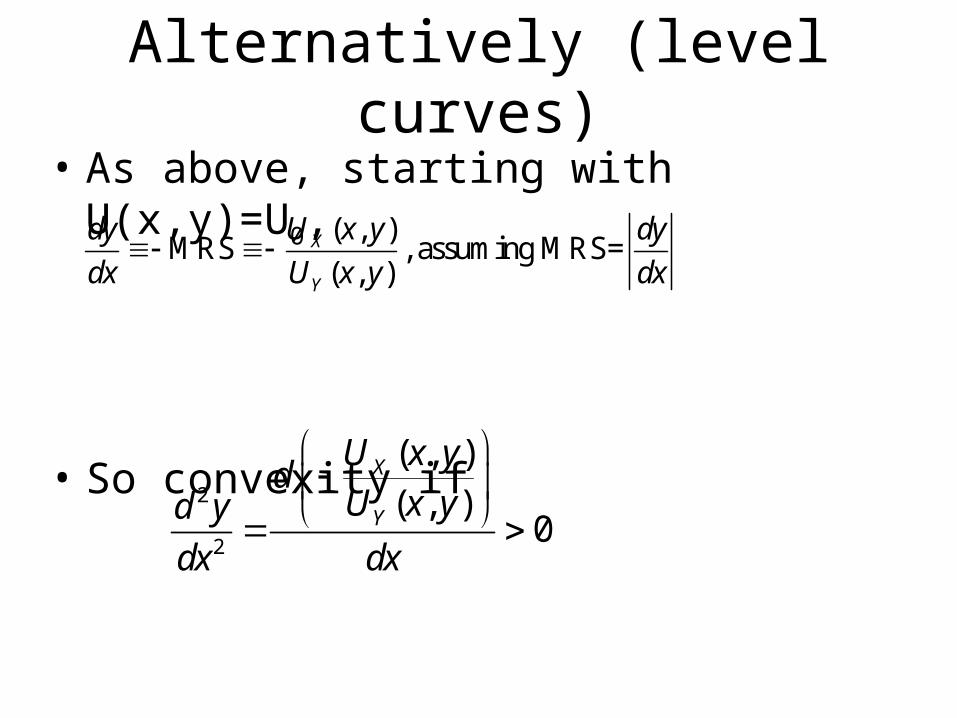
Alternatively (level curves)• As above, starting with U(x,y)=U0,
• So convexity if
( , )MRS , assuming MRS=
( , ) X
Y
U x ydy dy
dx U x y dx
2
2
( , )
( , )0
X
Y
U x yd
U x yd y
dx dx

Convexity (level curves)• And, that is
*Note that Uxx and Uyy need not be negative and Uy3>0
• What of:– Ux > 0, monotonacity, nonsatiation– Uy > 0, monotonacity, nonsatiation– Uxx, ?– Uyy, ?– Uxy, ?
2 22
2 3
( , )2( , )
0
X
xy x y y xx x yyY
y
U x yd
U U U U U U UU x yd y
dx dx U

Diminishing MU vs Diminishing MRS
• Both involve the idea of satiation. That is, the more you consume, the less you value added consumption.
• DMU: Consumption of other goods irrelevant• DMRS: The value of consuming additional units
of one good along an indifference curve falls because you are necessarily consuming less of other goods.
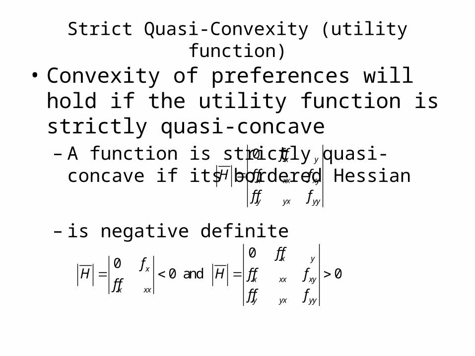
Strict Quasi-Convexity (utility function)• Convexity of preferences will hold if the utility
function is strictly quasi-concave– A function is strictly quasi-concave if its bordered
Hessian
– is negative definite
0 x y
x xx xy
y yx yy
f f
H f f f
f f f
00
0 and 0x y
xx xx xy
x xxy yx yy
f ff
H H f f ff f
f f f
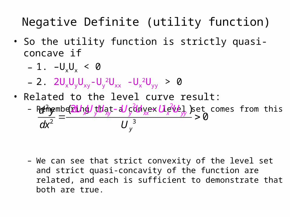
Negative Definite (utility function)• So the utility function is strictly quasi-concave if
– 1. –UxUx < 0
– 2. 2UxUyUxy-Uy2Uxx -Ux
2Uyy > 0
• Related to the level curve result:– Remembering that a convex level set comes from this
– We can see that strict convexity of the level set and strict quasi-concavity of the function are related, and each is sufficient to demonstrate that both are true.
2
2
2 2
3
2( )0
x y xy y x y
y
xx yU U U U U U Ud y
dx U
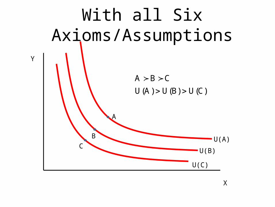
With all Six Axioms/Assumptions
Y
X
U(C)
U(B)
U(A)C
B
A
A B C
U(A) U(B) U(C)
Some Utility Functions and their Properties
• Homotheticity of Preferences• Elasticity of Substitution• Functional Forms
– CES– Cobb-Douglas– Perfect Substitutes– Perfect Compliments
Homothetic Preferences• The MRS depends only on the ratio of goods
consumed.• So any MRS that can be reduced so that x and y only
appear as the ratio (x/y) or (y/x) are considered homothetic.
• Changes in income lead to equal percent changes in consumption (income elasticity = 1 for all goods).
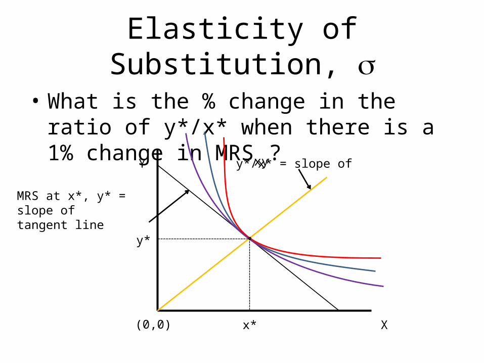
Elasticity of Substitution,
• What is the % change in the ratio of y*/x* when there is a 1% change in MRSxy?
Y
X
y*/x* = slope of
MRS at x*, y* = slope of tangent line
(0,0) x*
y*
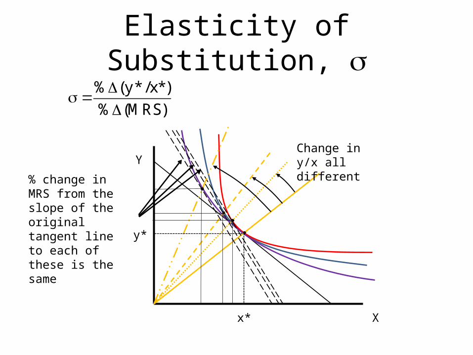
Elasticity of Substitution,
Y
X
Change in y/x all different
% change in MRS from the slope of the original tangent line to each of these is the same
% (y* /x*)
% (MRS)
x*
y*

Elasticity of Substitution, • As an elasticity, it is true that
• And, MRS = Ux/Uy
% (y* /x*) d(y* /x*) (MRS) d ln(y* /x*)
% (MRS) d(MRS) (y* /x*) d ln(MRS)
x
y
x x
y y
U x*, y*y* y*d d lnU x*, y*x * x *
y*U x*, y* U x*, y*d d lnx *U x*, y* U x*, y*
, or
Evaluated at (x*, y*)

And another substitution• And at utility maximizing x*and y*, MRS = px/py, so:
• Which means, elasticity of substitution can be defined as either of these:
• Which has some real economic meaning. It is a measure of the magnitude of the substitution effect.
x y
% (y* /x*) % (y* /x*)
% (MRS) % (p / p )
x
y
x x
y y
py* y*d d lnpx * x *
y*p pd d lnx *p p
, or

Utility Functions
• CES• Cobb-Douglas Utility• Perfect Substitutes• Perfect Compliments
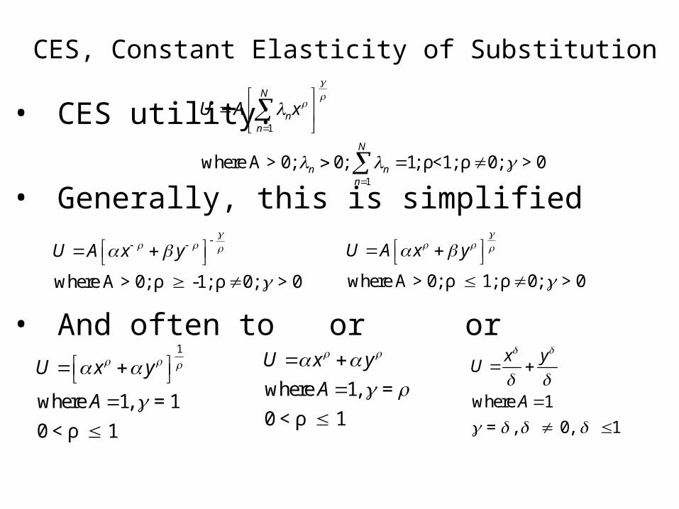
CES, Constant Elasticity of Substitution
• CES utility:
• Generally, this is simplified
• And often to or or
1
1
where A > 0; 0; 1; ρ<1; ρ 0; > 0
N
nn
N
n nn
U A x
where A > 0; ρ -1; ρ 0; > 0
U A x y
where 1, =
0 < ρ 1
U x y
A
1
where 1, = 1
0 < ρ 1
U x y
A
where 1
= , 0, 1
x yU
A
where A > 0; ρ 1; ρ 0; > 0
U A x y
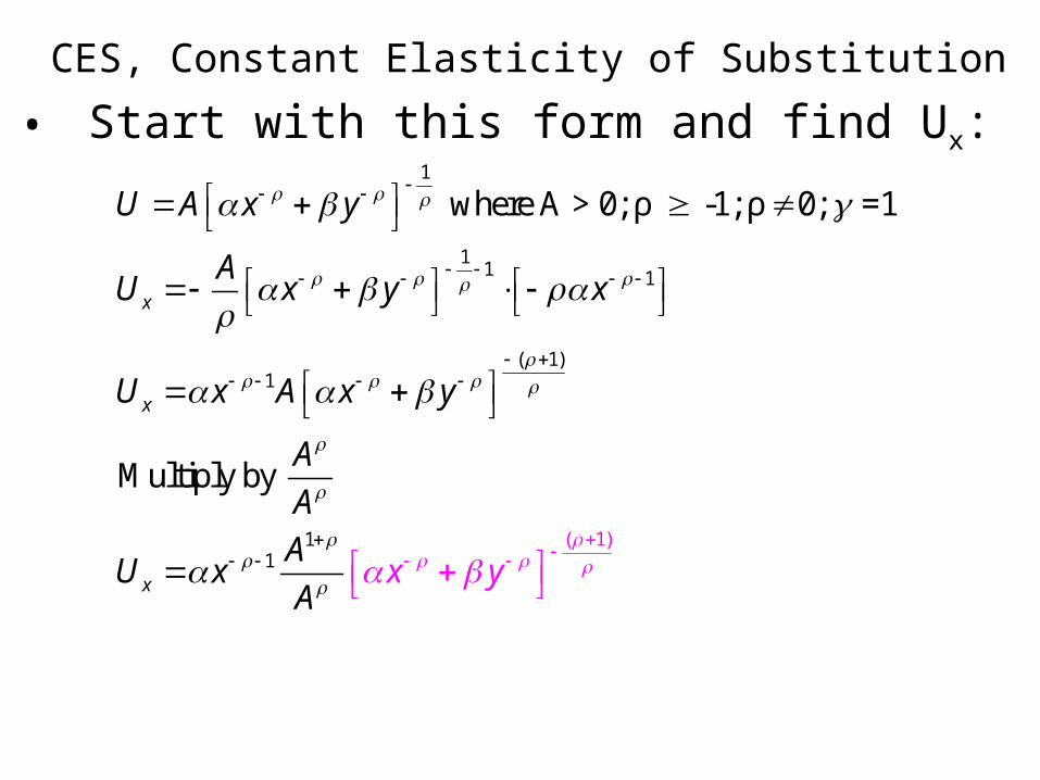
CES, Constant Elasticity of Substitution• Start with this form and find Ux:
(
1
11 1
( 1)1
1)11
where A > 0; ρ -1; ρ 0; =1
Multiply by
x
x
x
U A x y
AU x y x
U x A x y
A
A
x yA
U xA
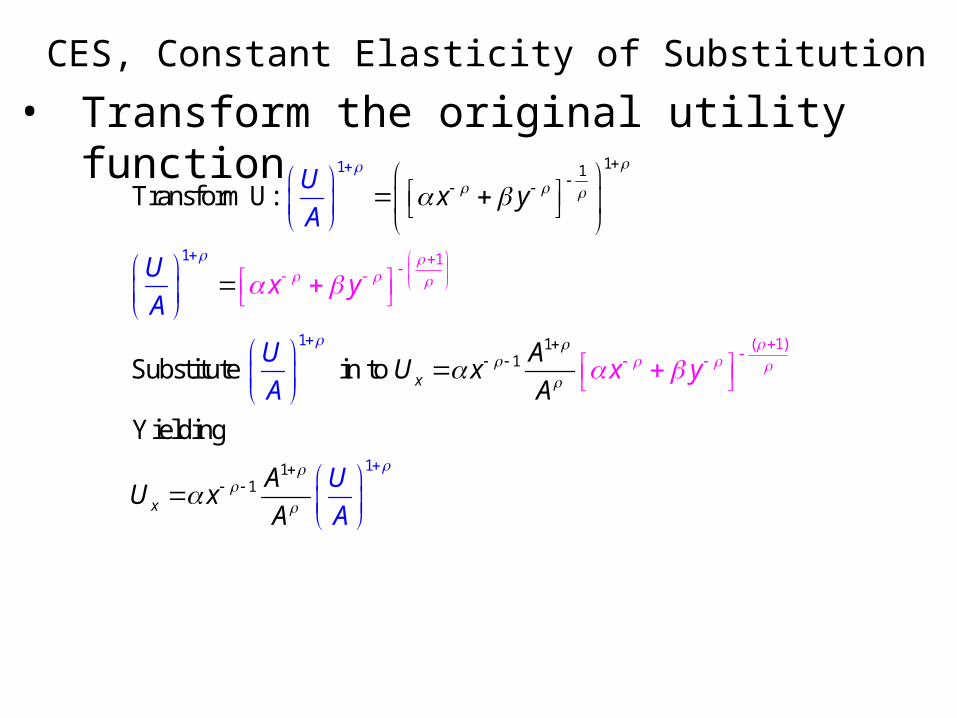
CES, Constant Elasticity of Substitution• Transform the original utility function
1
( 1)
1 11
11
1
1
11
1
Transform U:
Substitute in to
Yielding
x
x
x yU
A
U
A
U
A
U
A
AU x
A
x y
xA
y
AU
x
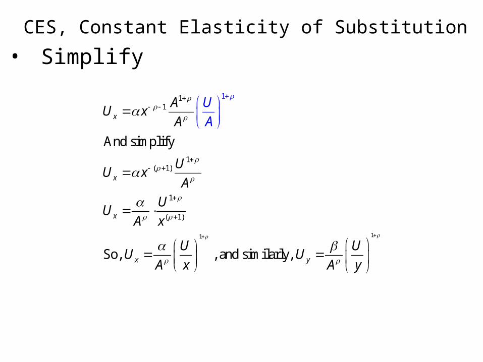
CES, Constant Elasticity of Substitution• Simplify
11
11
1( 1)
1
( )
1
1
And simplify
So, , and similarly,
x
x
x
x y
AU x
A
UU x
A
UU
A x
U UU
x A y
A
A
U
U

CES: MRS and σ• With Ux and Uy we can define MRS and σ:
*
*
*
*
MRS =
x
y
x
y
x
y
U
U
pyd
px
ypd
xp

CES: MRS1
1
1MRS =
x
y
UU yA xU xU
A y Homothetic!

CES: σ
1*
* **
*
1* 1
*
*
*
*
Utility max requires x and y such that:
So, at U-max:
x
y
x
x
y
y
y
x
pyd
px
ypd
xp
y
x p
p
p
py
x

CES: σ• Split it up:
*
*
1*
* 1
*
*
1
*
*
Split this into two parts, first deal with the derivative portion.
1
d
1
x
y
x
y
x
y
y
y
x
x
ydx
pdp
ydx
pdp
yx
p
pd
p
p
p
p
yx
1
11 111
1
x
y
p
p
*
*
*
*
1* 1
*, and
x
y
y
y
x
x
pyd
px
y
y
x
x ppdp
p
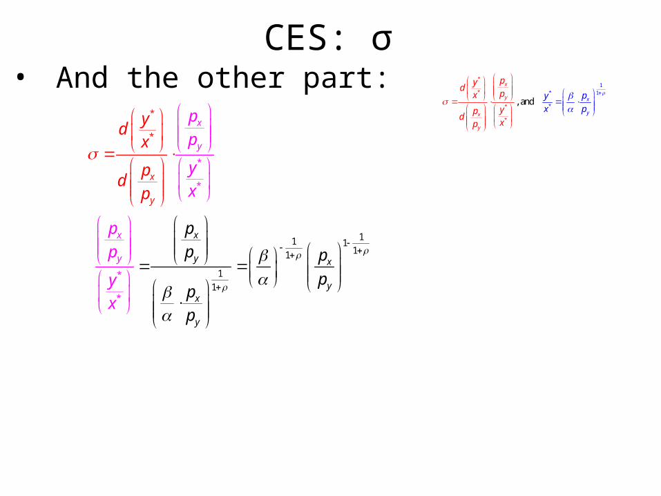
CES: σ• And the other part:
*
*
*
11 111
*
1
*
1*
x
y
x
y x
yx
y
x
x
y
y
p
p p
pp
p
p
p
yx
p
ydx
yx
d
p
p
p
*
*
*
*
1* 1
*, and
x
y
y
y
x
x
pyd
px
y
y
x
x ppdp
p
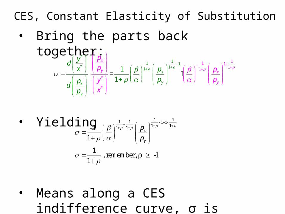
CES, Constant Elasticity of Substitution• Bring the parts back together:
• Yielding
• Means along a CES indifference curve, σ is constant… well named.
*11 1
11 11*
*
1
*
1 1=
1
1
x
y xx
yx
y
y
p
p p
p
ydx p
ppdp
yx
1 11 1 1 11 11 11
1
1, remember, ρ -1
1
x
y
p
p

CES: The Mother of All Utility Functions
1, -1, 0
1
As , 0, perfect compliments
As 0, 1, Cobb-Douglas
As 1, , perfect substitutes
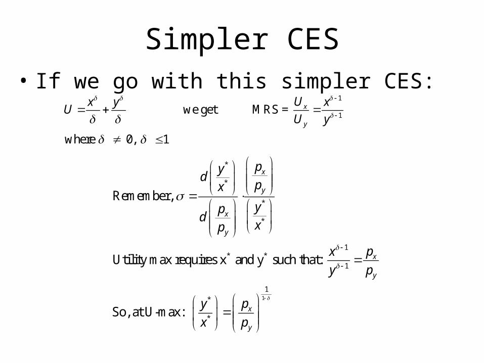
Simpler CES• If we go with this simpler CES:
1
1 we get MRS =
where 0, 1
x
y
Ux y xU
U y
1
*
*
*
*
1* *
1
1*
*
Remember,
Utility max requires x and y such that:
So, at U-max:
x
y
x
y
x
y
x
y
pyd
px
ypd
xp
px
y p
py
x p

Simpler CES• Which reduces to 1
11
11
1
11 1
1
1, here, 1, 0
1And this time
As , 0, perfect compliments
As 0, 1, Cobb-Douglas
As 1, , perfect substitutes
x
y
x
y
p
p
p
p

Cobb-Douglas• Cobb-Douglas: U = Axαyβ
• When 0<α<1 and 0<β<1 and α+β=1– α, share of income spent on x– β, share of income spent on y
• To get this, transform: UT = (U)(1/(α+β)) – UT = (xαyβ) 1/(α+β) – UT = (x(α/(α+β))y(β/(α+β))) – (α/α+β) + (β/α+β) = 1
• But how is Cobb-Douglas derived from CES?
MRSy
x
Homothetic
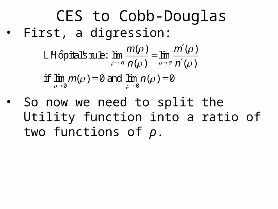
CES to Cobb-Douglas• First, a digression:
• So now we need to split the Utility function into a ratio of two functions of ρ.
0 0
( ) ( )ˆL'Hopital's rule: lim lim
( ) ( )
if lim ( ) 0 and lim ( ) 0
a a
m m
n n
m n

CES to Cobb-Douglas• Utility function:
• A monotonic transformation.
1
( ) where A > 0; ρ -1; ρ 0; 1
U A x y
T
T
T
1U = ln ln
1U = ln
lnU =
( ) ln
( )
Ux y
A
x y
x y
m x y
n
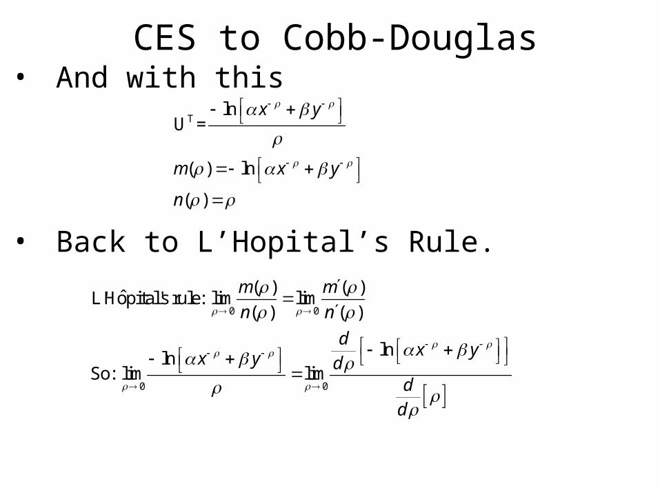
CES to Cobb-Douglas• And with this
• Back to L’Hopital’s Rule.
Tln
U =
( ) ln
( )
x y
m x y
n
0 0
0 0
( ) ( )ˆL'Hopital's rule: lim lim
( ) ( )
lnlnSo: lim lim
m m
n n
dx yx y ddd
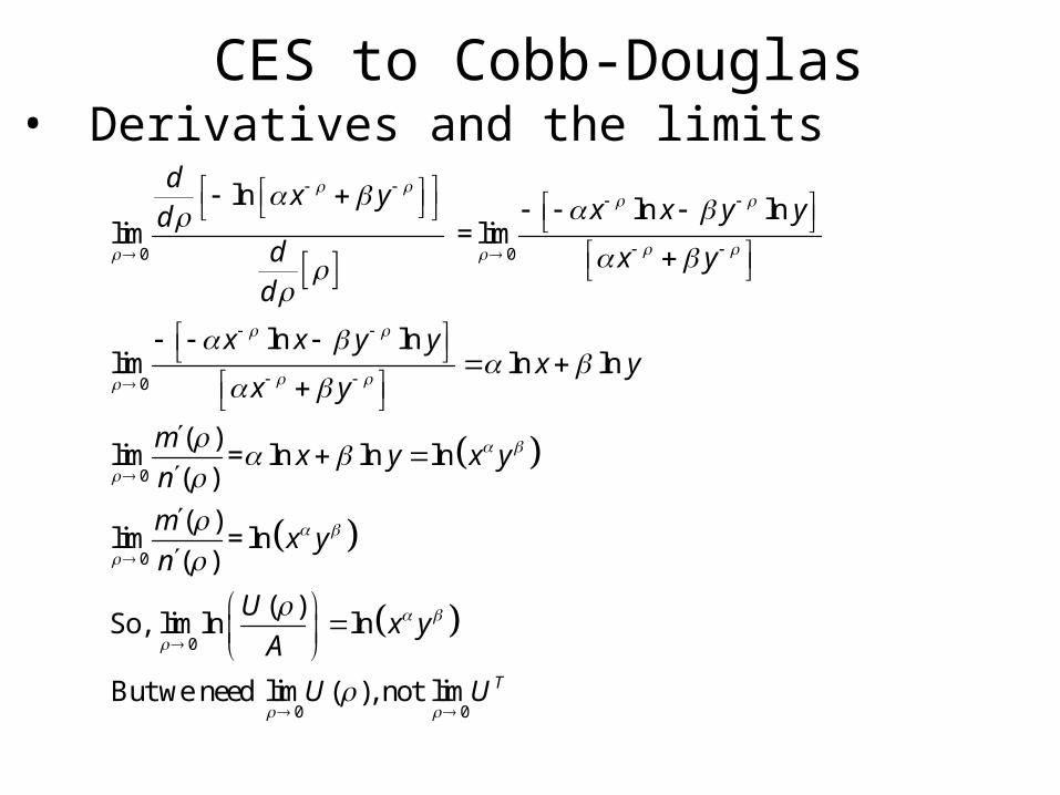
CES to Cobb-Douglas• Derivatives and the limits
0 0
0
0
0
0
ln ln lnlim = lim
ln lnlim ln ln
( )lim = ln ln ln
( )
( )lim = ln
( )
( )So, lim ln
dx y x x y ydd x yd
x x y yx y
x y
mx y x y
n
mx y
n
U
A
0 0
ln
But we need lim ( ), not lim
T
x y
U U

CES, Constant Elasticity of Substitution• A little rearranging:
• Yielding
• And so long as α+β=1, CES becomes Cobb-Douglas as ρ→0
0
0
0
l( )
lim ln
( ) ( )lim ln ln
0
0
( )l
n
l
0 0
im ln n
A
( )So, lim l
Ae
( )A
n
e lim lim li
ln
e =e
=
m ( )
e
U
Ux y
x y
U
A
A
U
A A
Ux
A
A
y
UA e A U
0
0
ln=Ae
l
l )
m ( )
m (
i
i
x yU
U Ax y
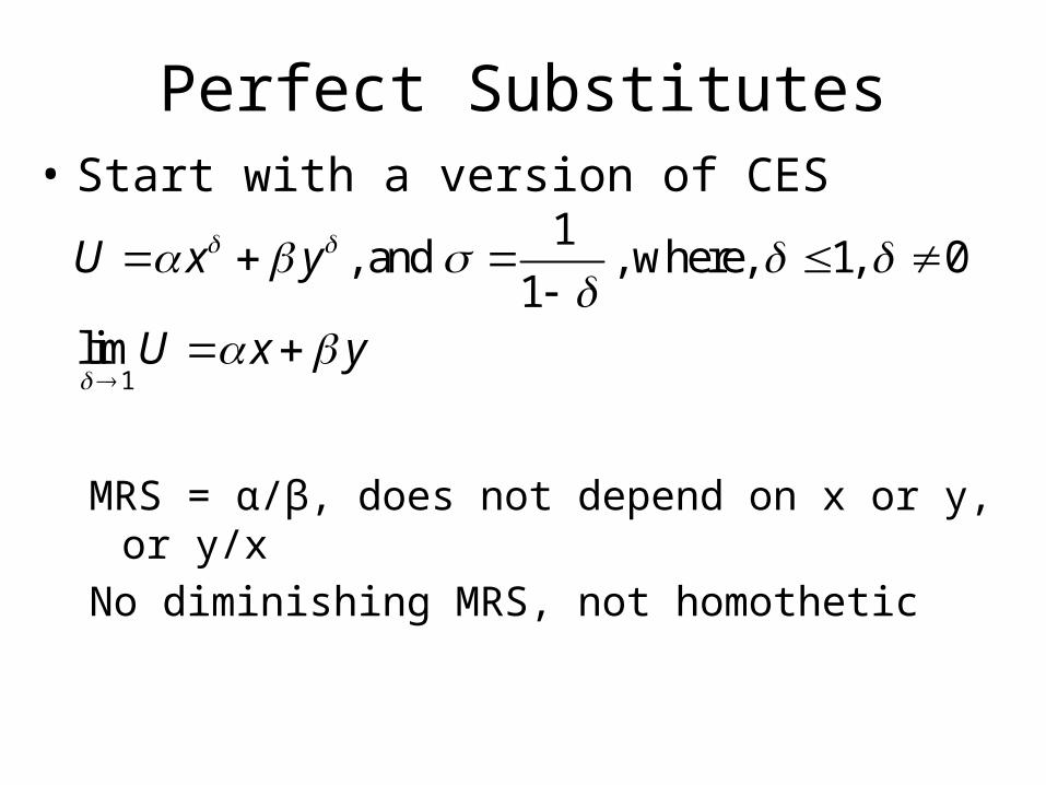
Perfect Substitutes• Start with a version of CES
MRS = α/β, does not depend on x or y, or y/xNo diminishing MRS, not homothetic
1
1, and , where, 1, 0
1lim
U x y
U x y
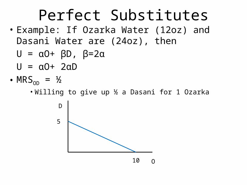
Perfect Substitutes• Example: If Ozarka Water (12oz) and Dasani Water are
(24oz), then U = αO+ βD, β=2αU = αO+ 2αD
• MRSOD = ½• Willing to give up ½ a Dasani for 1 Ozarka
O
D
10
5
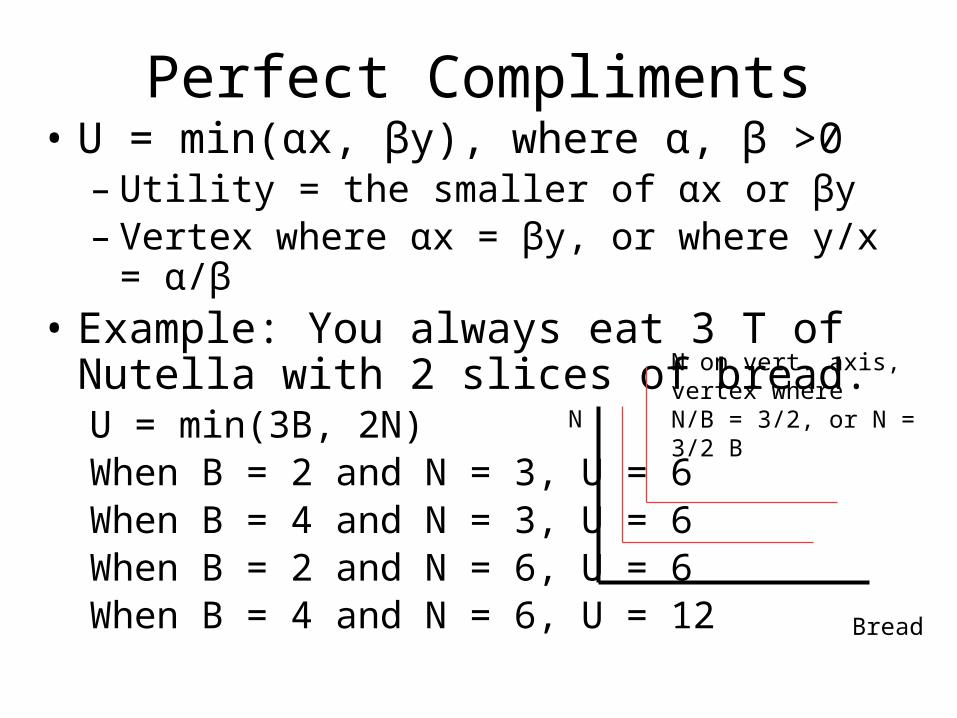
Perfect Compliments• U = min(αx, βy), where α, β >0
– Utility = the smaller of αx or βy– Vertex where αx = βy, or where y/x = α/β
• Example: You always eat 3 T of Nutella with 2 slices of bread.U = min(3B, 2N)When B = 2 and N = 3, U = 6When B = 4 and N = 3, U = 6When B = 2 and N = 6, U = 6When B = 4 and N = 6, U = 12
N on vert. axis, vertex whereN/B = 3/2, or N = 3/2 B
Bread
N

Neoclassical Behavioral Assertion• Consumers endeavor to maximize
where U(xi) represents the consumer’s own subjective evaluation of derived from the consumption of goods and services, xi.
• Under scarcity, consumers must choose among a limited set of bundles described by the budget constraint
where pi are the prices of xi goods and services and M is consumer income.
( )iU U x
i ip x M
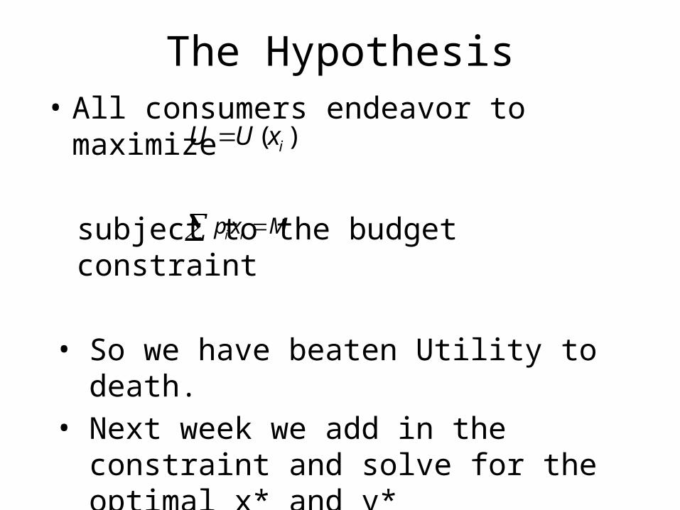
The Hypothesis• All consumers endeavor to maximize
subject to the budget constraint
• So we have beaten Utility to death. • Next week we add in the constraint and
solve for the optimal x* and y*
( )iU U x
i ip x M

Spare: MRS diminishing?• U = x+xy+y
o MRS = Ux/Uy = (1+y)/(1+x)o Is 2UxUyUxy-Uy
2Uxx -Ux2Uyy > 0 ?
o 2(1+y)(1+x)*1-(1+x)2*0-(1+y)2*0o 2(1+y)(1+x) > 0
• U = x2y2 o MRS = 2xy2/2x2y = y/xo Is 2UxUyUxy-Uy
2Uxx -Ux2Uyy>0 ?
o 2(2xy2)(2x2y)(4xy)-(4x4y2)(2y2)-(4x2y4)(2x2) > 0o 32x4y4 - 16x4y4 >0o 16x4y4 > 0

Diminishing MRS
x
xx xy y x yx yyy
2y
x
y
x x xxx xy y x yx yy
y y y
2y
xxx y xy x
y
U x, y dx dy dx dyd U U U U U UU x, y dx dx dx dx
dx U
UdyNote:
dx U
U x, y U Ud U U U U U U
U x, y U U
dx U
U x, yd U U U U
U x, y
dx
2x
yx x yyy
2y
y
y
x
2 2y xx y xy x y yx x y yy x
3y
x
2 2y xy x y xx y yy x
3y
UU U U
U
U
UMultiply by:
U
U x, yd
U x, y U U U U U U U U U U
dx U
U x, yd
U x, y 2U U U U U U U0
dx U