Embed Size (px)
Citation preview
Advanced MicroeconomicsExpected utility theory
Jan Hagemejer
January 5, 2010
Jan Hagemejer Advanced Microeconomics
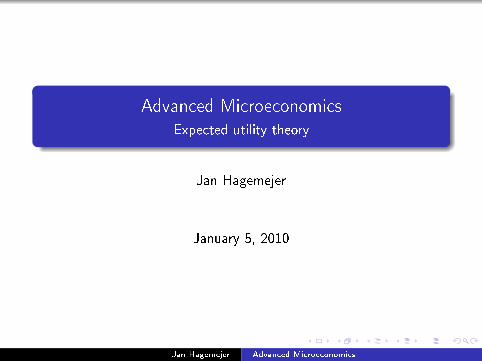
Introduction
C is a set of possible outcomes, consequences:
C could be monetary amounts
C could be consumption bundles (vectors of the amounts of
each commodities)
C could be:
a �nite set, with, say, N elements
a countably in�nite set
Example: C = {1,2,3, ...}
a continuum
Example: C = {x ∈ℜ|0≤ x ≤ 1}
Jan Hagemejer Advanced Microeconomics
A lottery
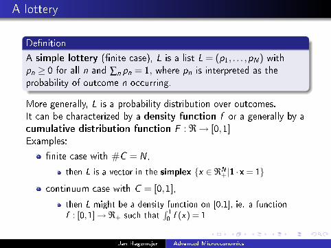
De�nition
A simple lottery (�nite case), L is a list L = (p1, . . . ,pN) with
pn ≥ 0 for all n and ∑n pn = 1, where pn is interpreted as the
probability of outcome n occurring.
More generally, L is a probability distribution over outcomes.
It can be characterized by a density function f or a generally by a
cumulative distribution function F : ℜ→ [0,1]Examples:
�nite case with #C = N,
then L is a vector in the simplex {x ∈ℜN+|1 ·x = 1}
continuum case with C = [0,1],
then L might be a density function on [0,1], ie. a functionf : [0,1]→ℜ+ such that
∫1
0f (x) = 1
Jan Hagemejer Advanced Microeconomics
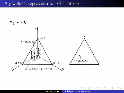
A graphical representation of a lottery
Figure 6.B.1
Jan Hagemejer Advanced Microeconomics
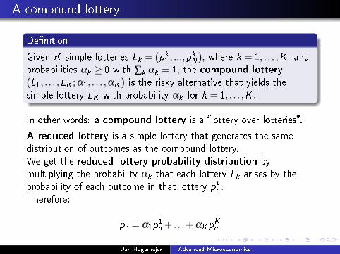
A compound lottery
De�nition
Given K simple lotteries Lk = (pk1, ...,pk
N), where k = 1, . . . ,K , and
probabilities αk ≥ 0 with ∑k αk = 1, the compound lottery(L1, . . . ,LK ;α1, . . . ,αK ) is the risky alternative that yields the
simple lottery LK with probability αk for k = 1, . . . ,K .
In other words: a compound lottery is a �lottery over lotteries�.
A reduced lottery is a simple lottery that generates the same
distribution of outcomes as the compound lottery.
We get the reduced lottery probability distribution by
multiplying the probability αk that each lottery Lk arises by the
probability of each outcome in that lottery pkn .Therefore:
pn = α1p1
n + . . .+ αKpK
n
Jan Hagemejer Advanced Microeconomics
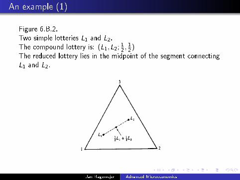
An example (1)
Figure 6.B.2.
Two simple lotteries L1 and L2.
The compound lottery is: (L1,L2; 12, 12
)The reduced lottery lies in the midpoint of the segment connecting
L1 and L2.
Jan Hagemejer Advanced Microeconomics
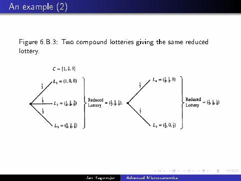
An example (2)
Figure 6.B.3: Two compound lotteries giving the same reduced
lottery.
Jan Hagemejer Advanced Microeconomics
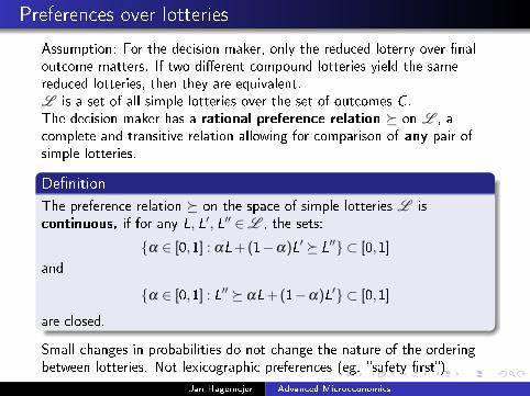
Preferences over lotteries
Assumption: For the decision maker, only the reduced loterry over �naloutcome matters. If two di�erent compound lotteries yield the samereduced lotteries, then they are equivalent.L is a set of all simple lotteries over the set of outcomes C .The decision maker has a rational preference relation � on L , acomplete and transitive relation allowing for comparison of any pair ofsimple lotteries.
De�nition
The preference relation � on the space of simple lotteries L iscontinuous, if for any L, L′, L′′ ∈L , the sets:
{α ∈ [0,1] : αL+ (1−α)L′ � L′′} ⊂ [0,1]
and
{α ∈ [0,1] : L′′ � αL+ (1−α)L′} ⊂ [0,1]
are closed.
Small changes in probabilities do not change the nature of the orderingbetween lotteries. Not lexicographic preferences (eg. �safety �rst�)
Jan Hagemejer Advanced Microeconomics
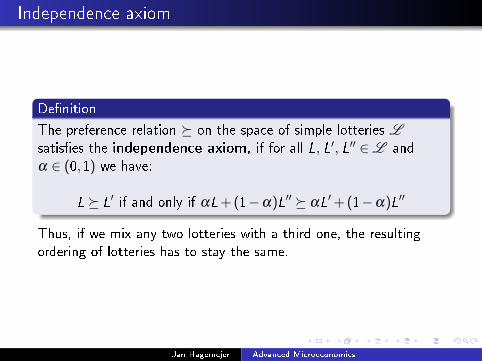
Independence axiom
De�nition
The preference relation � on the space of simple lotteries Lsatis�es the independence axiom, if for all L, L′, L′′ ∈L and
α ∈ (0,1) we have:
L� L′ if and only if αL+ (1−α)L′′ � αL′+ (1−α)L′′
Thus, if we mix any two lotteries with a third one, the resulting
ordering of lotteries has to stay the same.
Jan Hagemejer Advanced Microeconomics
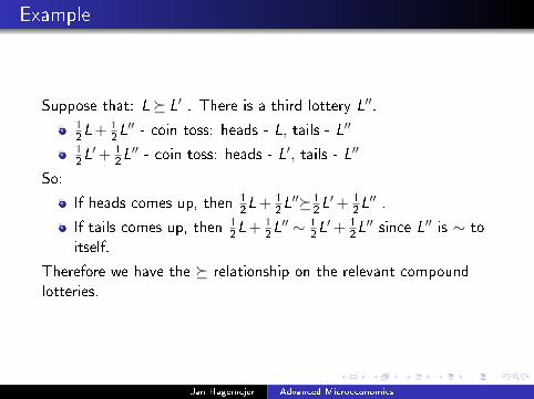
Example
Suppose that: L� L′ . There is a third lottery L′′.1
2L+ 1
2L′′ - coin toss: heads - L, tails - L′′
1
2L′+ 1
2L′′ - coin toss: heads - L′, tails - L′′
So:
If heads comes up, then 1
2L+ 1
2L′′�1
2L′+ 1
2L′′ .
If tails comes up, then 1
2L+ 1
2L′′ ∼ 1
2L′+ 1
2L′′ since L′′ is ∼ to
itself.
Therefore we have the � relationship on the relevant compound
lotteries.
Jan Hagemejer Advanced Microeconomics
Expected utility
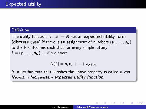
De�nition
The utility function U : L →ℜ has an expected utility form(discrete case) if there is an assignment of numbers (u1, . . . ,uN)to the N outcomes such that for every simple lottery
L = (p1, . . . ,pN) ∈L we have:
U(L) = u1p1 + ...+uNpN
A utility function that satis�es the above property is called a von
Neumann-Morgenstern expected utility function.
Jan Hagemejer Advanced Microeconomics
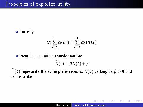
Properties of expected utility
linearity:
U(K
∑k=1
αkLk) =K
∑k=1
αkU(Lk)
invariance to a�ne transformations:
U(L) = βU(L) + γ
U(L) represents the same preferences as U(L) as long as β > 0 and
α are scalars.
Jan Hagemejer Advanced Microeconomics
Expected utility theorem
Theorem
If preferences satisfy continuity and independence, then they can be
represented by a von Neumann-Morgenstern utility function.
v.N-M representation means that indi�erence curves are
parallel lines
if indepedence is violated, indi�erence curves will not be
straight or will not be paralell.
Jan Hagemejer Advanced Microeconomics
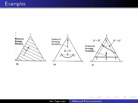
Examples
Jan Hagemejer Advanced Microeconomics
Problems
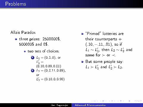
Allais Paradox
three prizes: 2500000$,
500000$ and 0$.
two sets of choices:
1 L1 = (0,1,0), orL′1
=(0.10,0.89,0.01)
2 L2 = (0,0.11,0.89),or
L′2
= (0.10,0,0.90)
�Primed� lotteries are
their counterparts +
(.10,−.11, .01), so if
L1 ∼ L′1, then L2 ∼ L′
2and
same for � or ≺.But some people say:
L1 � L′1and L′
2� L2.
Jan Hagemejer Advanced Microeconomics
Problems
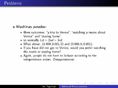
Machinas paradox:
three outcomes: �a trip to Venice�, �watching a movie aboutVenice� and �staying home�.so normally 1st � 2nd � 3rd .What about: (0.999,0.001,0) and (0.999,0,0.001).If you have did not get to Venice, would you prefer watchingthe movie or staying home?Again, people do not have to behave according to theindependence axiom. Dissapointemnt.
Jan Hagemejer Advanced Microeconomics
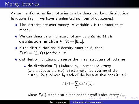
Money lotteries
As we mentioned earlier, lotteries can be described by a distribution
functions (eg. if we have a unlimited number of outcomes).
The lotteries are over money. A variable x is the amount of
money.
We can describe a monetary lottery by a cumulativedistribution function F : ℜ→ [0,1].
if the distribution has a density function f , then
F (x) =∫x
−∞f (t)dt for all x .
distribution functions preserve the linear structure of lotteries:
the distribution F (.) induced by a compound lottery(L1, . . . ,LK ;α1, . . . ,αK ) is just a weighted average of thedistributions induced by each of the lotteries that constitute it:
F (x) = ∑k
αkFk(x),
where Fk(.) is the distribution of the payo� under lottery Lk .
Jan Hagemejer Advanced Microeconomics
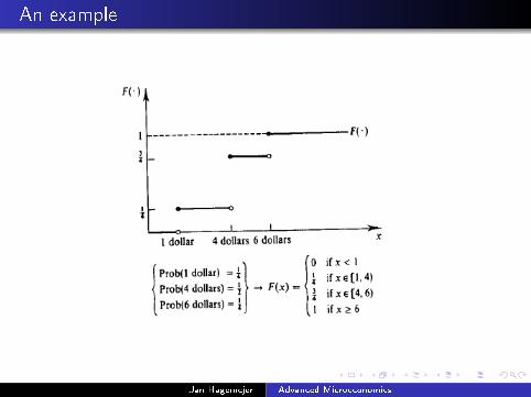
An example
Jan Hagemejer Advanced Microeconomics
Some de�nitions
a lottery is nondegenerate if the probability distribution is
non degenerate, that is:
0 < F (x) < 1 for some x
a lottery is fair if its expected value (∫
∞
−∞xdF (x)) is 0.
Jan Hagemejer Advanced Microeconomics
The expected utility function
The von Neumann-Morgenstern expected utility function takes
the form:
U(F ) =∫u(x)dF (x),
so U(f ) is the expected value of the utility over the
distribution of all possible realisations of x (not to be confused
with the expected value of x which is expressed as
U(F ) =∫xdF (x)).
Mas-Colell convention - the v.N-M function is the U and the u
is the Bernoulli utility function (some people call u the v.N-M).
u(x) is the utility of getting the amount x with certainty.
Jan Hagemejer Advanced Microeconomics
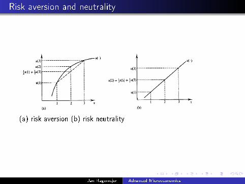
Risk aversion and neutrality
De�nition
A decision maker is a risk averter (or exhibits risk aversion) if iffor any lottery F (.) the degenerate lottery that yields the amount∫xdF (x) (expected value of x) with certainty is at least as good as
the lottery F (.) itself.
He is risk neutral if he is indi�erent over the two lotteries.
He is strictly risk averse if and only if the indi�erence holds if the
two lotteries are the same.
In other words: a risk averse agent would reject any nondegenerate
fair lottery given its wealth level.
A risk neutral - indi�erent.
A risk lover - prefer the lotteries.
These are global.
Jan Hagemejer Advanced Microeconomics
Risk aversion (2)
If preferences admit an expected utility representation with a
Bernoulli function u(x), then risk aversion i�:∫u(x)dF (x)≤ u(
∫xdF (x)) for all F (.).
The above is called Jensen inequality � a de�ning property of a
concave function.
Jan Hagemejer Advanced Microeconomics
Risk aversion and neutrality
(a) risk aversion (b) risk neutrality
Jan Hagemejer Advanced Microeconomics
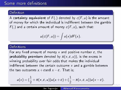
Some more de�nitions
De�nition
A certainty equivalent of F (.) denoted by c(F ,u) is the amount
of money for which the individual is indi�erent between the gamble
F (.) and a certain amount of money c(F ,u), such that:
u(c(F ,u)) =∫u(x)dF (x).
De�nitions
For any �xed amount of money x and positive number ε, theprobability premium denoted by π(x ,ε,u)), is the excess inwinning probability over fair odds that makes the individual
indi�erent between the certain outcome x and a gamble between
the two outcomes x + εand x− ε . That is:
u(x) = (1
2+ π(x ,ε,u))u(x + ε) + (
1
2−π(x ,ε,u))u(x− ε).
Jan Hagemejer Advanced Microeconomics
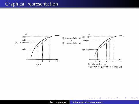
Graphical representation
Jan Hagemejer Advanced Microeconomics
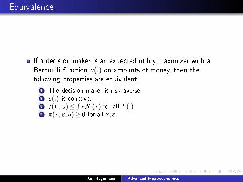
Equivalence
If a decision maker is an expected utility maximizer with a
Bernoulli function u(.) on amounts of money, then the
following properties are equivalent:
1 The decision maker is risk averse.2 u(.) is concave.3 c(F ,u)≤
∫xdF (x) for all F (.).
4 π(x ,ε,u)≥ 0 for all x ,ε.
Jan Hagemejer Advanced Microeconomics
The Arrow-Pratt coe�cient
The Arrow-Pratt coe�cent of absolute risk aversion at point x
is de�ned as:
rA(x) =−u′′(x)
u′(x).
The risk aversion coe�cent measures the curvature of u. Thecloser the u is to a linear function, the less risk averse the
agent is.
The nice feature of r is that it is invariant to positive linear
transformations of u.
r measures how the probability premium increases at certainty
rA(x) = 4π′(x ,0,u)
Jan Hagemejer Advanced Microeconomics
Comparing individuals
Given two utility functions, u2 is more risk averse than u1 if:
1 rA(x ,u2)≥ rA(x ,u1) for every x .
2 There exists an increasing concave function ψ(.) such that
u2(x) = ψ(u1(x)) at all x .
3 c(F ,u2)≤ c(F ,u1) for any F (.).
4 π(x ,ε,u2)≥ π(x ,ε,u1) for any x and ε.
5 Whenever 2 �nds a lottery F (.) as good as riskless outcome x ,
then 2 also �nds F (.) at least as good as x .
Jan Hagemejer Advanced Microeconomics
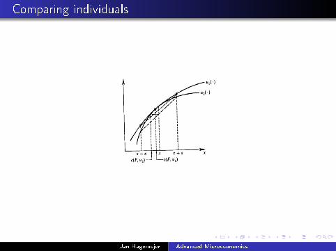
Comparing individuals
Jan Hagemejer Advanced Microeconomics
Coe�cient of relative risk aversion
De�nition
The coe�cient of relative risk aversion at point x is de�ned as:
rR(x) =−x u′′(x)
u′(x).
Decreasing relative risk aversion (RRA) means that as wealth
increases, the individual becomes less risk averse with respect
to gambles that are the same in proportion to his wealth.
Also, decreasing RRA implies decreasing ARA, so with the
increase in wealth the individual becomes less risk averse to
the gambles that are of the same absolute size.
Jan Hagemejer Advanced Microeconomics
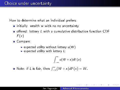
Choice under uncertainty
How to determine what an individual prefers:
initially: wealth w with no no uncertainty
o�ered: lottery L with a cumulative distribution function CDF
F (x)
Compare:
expected utility without lottery u(W )expected utility with lottery L:∫
∞
−∞
u(W + x)dF (x)
Note: if L is fair, then∫
∞
−∞(W + x)dF (x) = W .
Jan Hagemejer Advanced Microeconomics
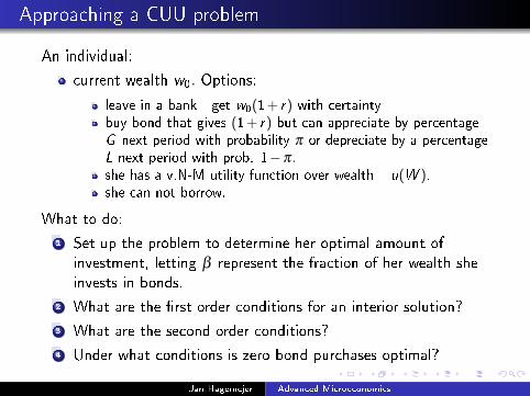
Approaching a CUU problem
An individual:
current wealth w0. Options:
leave in a bank - get w0(1+ r) with certaintybuy bond that gives (1+ r) but can appreciate by percentageG next period with probability π or depreciate by a percentageL next period with prob. 1−π.she has a v.N-M utility function over wealth � u(W ).she can not borrow.
What to do:
1 Set up the problem to determine her optimal amount of
investment, letting β represent the fraction of her wealth she
invests in bonds.
2 What are the �rst order conditions for an interior solution?
3 What are the second order conditions?
4 Under what conditions is zero bond purchases optimal?
Jan Hagemejer Advanced Microeconomics
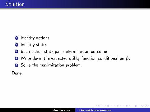
Solution
1 Identify actions
2 Identify states
3 Each action-state pair determines an outcome
4 Write down the expected utility function conditional on β .
5 Solve the maximization problem.
Done.
Jan Hagemejer Advanced Microeconomics
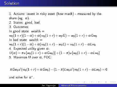
Solution
1. Actions: invest in risky asset (how much) - measured by the
share (eg. α).
2. States: good, bad.
3. Outcomes:
In good state: wealth =
w0(1+ r)(1−α) + α(w0(1+ r) +w0G ) = w0(1+ r) + αGw0
In bad state: wealth =
w0(1+ r)(1−α) + α(w0(1+ r)−w0L) = w0(1+ r)−αLw0
4. Expected utility given α :
U(α) = πu [w0(1+ r) + αGw0)] + (1−π)u [w0(1+ r)−αLw0]5. Maximize U over α , FOC:
πGw0u′(w0(1+ r) + αGw0)− (1−π)Lw0u
′(w0(1+ r)−αLw0) = 0
and solve for α∗.
Jan Hagemejer Advanced Microeconomics
Solution (2)
6. Second order condition?
U ′′(α∗)≤ 0
7. When is zero bond purchase optimal?
U ′(α = 0)≤ 0
When marginal expected utility at zero purchase is either zero or
negative.
Jan Hagemejer Advanced Microeconomics
Comparison of payo�s distribution
So far we have been comparing individuals and their preferences
towards risk.
Now we compare the lotteries with respect to:
level of returns
dispersion of returns
These correspond to:
�rst order stochastic dominance
second order stochastic dominance
We restrict our attention to cases of F (.) such that F (0) = 0 and
F (x) = 1 for some x .
Jan Hagemejer Advanced Microeconomics
Comparison of payo�s distribution
These concepts are important because they can be helpful to
determine what a risk averse individual would choose even if we
do not know his exact preferences.
Why?
�rst order stochastic dominance - one lottery �rst order
dominates another if it gives unambiguously higher returns
than the other.
second order stochastic dominance - one lottery second order
dominates another when the returns are the same but the
lottery has smaller spread (risk).
Jan Hagemejer Advanced Microeconomics
First order stochastic dominance
De�nition
We say that distribution F (.) �rst order stochasticallydominates G (.) if for every nondecreasing function u : ∑R→ R,
we have: ∫u(x)dF (x)≥
∫u(x)dG (x)
Proposition
The distribution of monetary payo�s F (.) �rst order stochastically
dominates the distribution G (.) if and only if F (x)≤ G (x) for every
x.
Jan Hagemejer Advanced Microeconomics
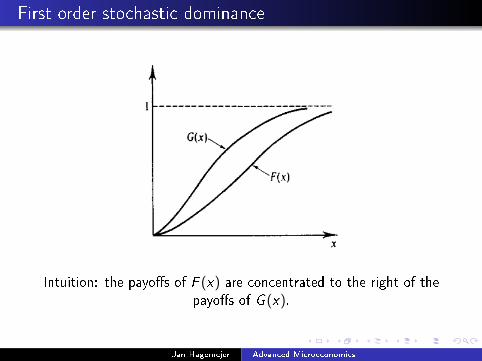
First order stochastic dominance
Intuition: the payo�s of F (x) are concentrated to the right of the
payo�s of G (x).
Jan Hagemejer Advanced Microeconomics
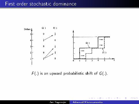
First order stochastic dominance
F (.) is an upward probabilistic shift of G (.).
Jan Hagemejer Advanced Microeconomics
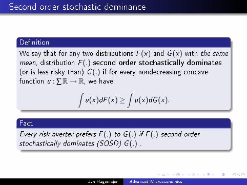
Second order stochastic dominance
De�nition
We say that for any two distributions F (x) and G (x) with the same
mean, distribution F (.) second order stochastically dominates(or is less risky than) G (.) if for every nondecreasing concave
function u : ∑R→ R, we have:∫u(x)dF (x)≥
∫u(x)dG (x).
Fact
Every risk averter prefers F (.) to G (.) if F (.) second order
stochastically dominates (SOSD) G (.) .
Jan Hagemejer Advanced Microeconomics
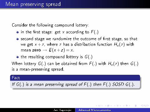
Mean preserving spread
Consider the following compound lottery:
in the �rst stage: get x according to F (.)
second stage we randomize the outcome of �rst stage, so that
we get x + z , where z has a distribution function Hx(z) with
mean zero → E (x + z) = x .
the resulting compound lottery is G (.)
When lottery G (.) can be obtained from F (.) with Hx(z) then G (.)is a mean-preserving spread.
Fact
If G (.) is a mean preserving spread of F (.) then F (.) SOSD G (.).
Jan Hagemejer Advanced Microeconomics
Second order stochastic dominance
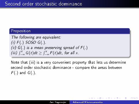
Proposition
The following are equivalent:
(i) F (.) SOSD G (.).(ii) G (.) is a mean preserving spread of F (.)(iii)
∫x
−∞G (t)dt ≥
∫x
−∞F (t)dt, for all x.
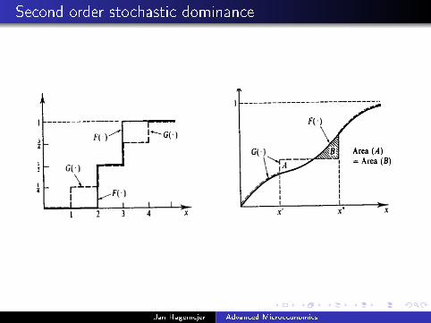
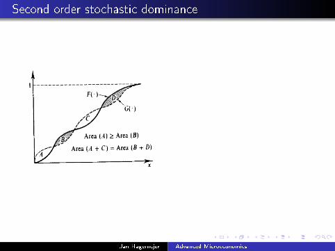
Note that (iii) is a very convenient property that lets us determine
second order stochastic dominance - compare the areas between
F (.) and G (.).
Jan Hagemejer Advanced Microeconomics
Second order stochastic dominance
Jan Hagemejer Advanced Microeconomics
Second order stochastic dominance
Jan Hagemejer Advanced Microeconomics