1

Advanced Multiphase Modeling of Solidification

with OpenFOAM®

A. Vakhrushev1, A. Ludwig

2, M. Wu

1, Y. Tang

3, G. Hackl

3, G. Nitzl

4

1 Christian Doppler Laboratory for Advanced Process Simulation of Solidification and Melting,

University of Leoben, 8700 Leoben, Austria 2 Simulation and Modeling of Metallurgical Processes, Department of Metallurgy, University of

Leoben, 8700 Leoben, Austria 3 RHI AG, Technology Center, Magnesitstrasse 2, 8700 Leoben, Austria

4 RHI AG, 1100 Vienna, Wienerbergstrasse 9, Austria

Abstract

Accumulated results of using OpenFOAM® as a tool to simulate various phenomena

accompanying casting processes are presented in this paper. The designed solidification

model incorporates mass and heat transfer along with the description of the multiphase solid /

liquid region being formed as a porous media [1]. Turbulent flow interaction with the so

called “mushy zone” is taken into account and its influence on the solid shell formation is

examined extending results of reference [2,3]. Motion of the different non-metallic inclusions

is modeled within the Lagrangian frame of reference [4] and verified with the experimental

data. A new approach of modeling elastic deformations of the solid shell during the withdraw

process in the funnel-shaped mold types is proposed as a supplement to improve the algorithm

with local numerical mesh refinement presented in [5].

Keywords

Solidification, discrete phase, turbulence, deformations.

1. INTRODUCTION

Multiphase flow phenomenon is of the great interest for the modern CFD field investigations,

taking into account phase transition process as well as the momentum and energy exchange

between the phases. These tasks can be solved in the most complex case by incorporating the

full set of the Navier-Stokes equations for each of the single phases being under the

consideration. This is so called Eulerian approach, where the description of the velocity,

density, temperature, solid fraction and other simulated fields focuses on the specific locations

in the space through which the multiphase flow advances with the course of time.

Presented studies incorporate modeling results for the around-casting processes, such as

dendritic solidification, motion of the non-metallic inclusions and gas bubbles within the melt.

The newest investigations here concern stress-and-strain analysis in the solidified shell.

An enthalpy-based mixture solidification model with consideration of turbulent flow [6-9]

was introduced by the current authors to model conventional continuous casting [4,10].

According to Voller et al., the treatment of the motion of the solid phase has a dramatic

influence on the convection of the latent heat, hence on the shape of the evolving mushy zone

[11-14]. New continuous casting technologies, e.g. the thin slab casting (TSC), for their

advantages of integration of the casting-rolling production chain, energy saving, high

productivity and near net shape, is likely to replace the conventional slab casting for

2

producing flat/strip products [15,16]. However, the frequently reported problems like the

sensibility to breakout and edge/surface cracks have challenged the metallurgists to consider

modeling tools to optimize and control the TSC parameters [17-19]. The key issue for the

modelling is to consider the evolution of the solid shell, which interacts strongly with the

turbulent flow and in the meantime is subject to continuous deformation due to the funnel

shape (curvature) of the mould. Model formulation and the analysis of the simulation results

are presented here.

During modeling of the turbulent flows and solidification in the continuous casting process to

tackle particles and gas bubbles motion, Lagrangian method gives a huge advantage if it is

exploited for the simulation of the additional phases with the relatively small volume fraction

(<10%). Thereby, diverse nonmetallic inclusions and small gas bubbles can be described

within Lagrangian frame of the reference. In the presented work the results of studies,

obtained using commercial CFD software FLUENT, are compared with the comprehensive

experimental measurements and with the simulations using OpenFOAM® solver, designed by

the authors, incorporating the Discrete Phase Model (DPM) and Discrete Random Walk

(DRW) models [4,20,21].

Momentum exchange between continuous and discrete phase, which is rather important for

the transient simulation of the nonmetallic inclusions and gas bubbles motion during

continuous casting, is taken into account by means of two-way coupling technique.

The advantage of the presented models consists of open-source implementation using

OpenFOAM® CFD software package, which permits to combine different multiphase sub-

models and to apply for the multiphase simulations.

2. SOLIDIFICATION MODEL

An enthalpy-based mixture solidification model [11-13] is applied. This mixture combines

liquid -phase and solid s-phase, which are quantified by their volume fractions, f ands

f .

The morphology of the solid phase is usually dendritic, but here we consider the dendritic

solid phase as a part of the mixture continuum. The mixture continuum changes continuously

from a pure liquid region, through the mushy zone (two phase region), to the complete solid

region. The evolution of the solid phase is determined by the temperature according to a

Tf s

relation (e.g. Gulliver-Scheil),

1

1

0

1

1

liquidusff pks TTTTf

.Eutectic

Eutecticliquidus

liquidus

TT

TTT

TT

(1)

Only one set of Navier-Stokes equation, which is applied to the domain of the bulk melt and

mushy zone, is solved in the Eulerian frame of reference.

0 u

, (2)

uu

t

u

moneff )( Sup

, (3)

3

where

s

ss

u

ufuf

u

u

region. solid

zonemushy

regionmelt bulk

(4)

Here s

u

, the solid velocity, is estimated by solving volume conservation and Laplace’s

equations (see below). The momentum sink due to the drag of the solid dendrites in the

mushy zone is modeled by the Blake-Kozeny law:

)( smon uuK

S

(5)

The permeability, K, is modeled as function of the primary dendrite arm spacing1

[22]:

2

1

4

2

s

3

106

f

fK . (6)

The energy equation applies to the entire domain,

eeff

SThut

h

. (7)

Here h is the sensible enthalpy of the solid s

h ref

h dTcT

T refp

. At a given temperature the

liquid phase is assumed to have an enthalpy of Lhh s . Release of latent heat by

solidification, L, is treated in the source term of the energy equation,

tfLS se

ssufL

. (8)

3. TURBULENT FLOW MODEL FOR SOLIDIFICATION

A low Reynolds number k - model was introduced by Prescott and Incropera [6-9] to

handle the turbulence during solidification. In current studies a realizable k - model was

employed providing improved performance for flows involving boundary layers under strong

pressure gradients and strong streamline curvature. The governing equations for the

turbulence are

k

KGkku

t

k

kt,

t

Pr, (9)

kCSCu

t

2

21

t,

t

Pr

, (10)

The turbulent Prandtl numbers for k : kt,

Pr =1.0, and for : t,Pr =1.2; G is the shear

production of turbulence kinetic energy; ijijSSS 2 , jiijij

xuxuS 5.0 ; /kS

. A simple approach is used to modify the turbulence kinetic energy in the mushy zone. It is

assumed that within a coherent mushy zone turbulence is dampened by shear which is linearly

4

correlated with the reduction of the mush permeability. The influence of turbulence on the

momentum and energy transports are considered by the effective viscosity, teff

, and

the effective thermal conductivity, teff , where 2

μtkC ,

ht,p,ttPr cf ,

μC

is a function of velocity gradient and ensures positivity of normal stresses; ht,

Pr is the

turbulent Prandtl number for energy equation (0.85).

4. VELOCITIES IN THE DEFORMING SHELL

A linear elasticity model [23] is further simplified to estimate the solid velocity. If we assume

that in the solid domain the elastostatics condition applies and the body force is ignorable, the

governing equation obtained is called Navier-Cauchy equation or elastostatic equation:

0

, (11)

where

is the displacement vector. So called Lamé parameters , are

12,

211

EE, (12)

where E represents Young's modulus and is Poisson’s ratio. If the solid shell is

incompressible and its deformation is at small strains ( 5.0 ), then a volume conservation

condition is fulfilled:

0

, (13)

and the first term of Eq. (11) is forced to zero as well:

0

. (14)

Transforming Eq.(13) and (14) from Lagragian frame into Eulerian frame by considering

tu

s, we obtain volume-conserved Laplace’s equations:

.0

,0

s

s

u

u

(15)

In 2D case, these volume-conserved Laplace’s equations can be solved with a method

(Method I) [24]. A stream function and a curl of the solid velocity s

u

are defined

by:

y

u

x

u

xu

yu

x

s

y

sy

s

x

s,,

, (16)

with Tuuu ),( y

s

x

ss

. Therefore, corresponding system of Eq. (15) can be written in form of:

5

.0

,

2

2

2

2

2

2

2

2

yx

yx

(17)

This method provides accurate solution, but it applies only to the 2D case. An

alternative and approximation method (Method II), applicable to both 2D and 3D, is to solve

the one-phase Navier-Stokes equation with an ‘infinite solid viscosity’. In the current work

the approximation method is to be justified by comparison with the method on the 2D

base.

5. MODELING DISCRETE PHASE

The inclusions and bubbles motion along with a highly turbulent flow are under consideration

in the presented numerical model. To specify the continuous phase motion, a fixed finite

volume mesh is used with a so-called collocated or non-staggered variable arrangement (Rhie

and Chow [25], Perić [26]), where all physical values share the same control volumes (CV),

and all flux variables reside on the CV faces. The generalized form of the divergence theorem

is used throughout the discretization procedure to represent mass and momentum

conservation laws in integral form over the control volume. Nonmetallic inclusions and gas

bubbles hereinafter referred to as “Lagrangian particles” and representing the discrete phase

are tracked within Lagrangian framework.

The Navier-Stokes equations with an assumption of the liquid incompressibility are used to

simulate the liquid melt motion. The equation system consisting of the continuity and

momentum equations is

0 u

, (18)

uu

t

u

Peff )( Sup

, (19)

The presence of the discrete phase is defined by the source term pS

, which represents the

momentum exchange between Lagrangian particles and the liquid flow. The estimation of its

quantitative evaluation is described later. In the presented study, a RANS turbulence approach

is used based on k model.

To employ the DPM theory, a definition of the Lagrangian particle should be introduced.

Hereinafter we consider a spherical particle with the diameter PD and the density P . Thereby

the mass of the particle with the volume PV is estimated as

3

PPPPP6

1DVm . (20)

Next, it is required to track the antecedent particles’ trajectories through the simulation

domain. Thereto each Lagrangian object is provided with its own position vector Px

in the

Cartesian system of coordinates. To determine the particle’s velocity Pu

and the

6

corresponding acceleration Pa

, it is sufficient to compute the time derivatives of the

trajectory vector Px

of the corresponding order:

PPP xua . (21)

The defining equation of the motion in the Lagrangian frame is based on the Newton’s

Second Law. It binds the acceleration of the particle with the resulting forces, acting on it:

PFum

P , (22)

where a sum of the external forces PF

originate in the influence from other Lagrangian

particles as well as in the impact from the surrounding continuous media motion.

A number of the forces are taken into account in the presented work: particles drag,

gravitational force, lift force, virtual mass force as well as pressure and stress gradient forces.

For the detailed formulation and description of each force please refer to publication [4].

It should be noticed, that drag coefficient in the model depends on the flow regime around the

discrete particle (see Figure 1) for the proper description of the inclusions behavior in the

turbulent flow.

Figure 1: Spherical particles drag law

To represent the particle / solid wall interaction the bouncing model is defined by the

restitution factor wall and the wall friction coefficient wall . Splitting the particle velocity

vector into the normal n

Pu

and the tangential τ

Pu

components, one can achieve a new particle

velocity *

Pu

after its interaction with the firm surface:

.uμu

,uεu

,uuu

τ

Pwall

τ

P

n

Pwall

n

P

τ

P

n

PP

1*

*

***

(23)

7

Figure 2: Interaction of Lagrangian particles with continuous phase

To couple the momentum in the both phase, the momentum exchange is determined in each

finite volume of the numerical mesh being used for the continuous phase (see Figure 2). For

the mesh element with the index k and of the volume kV the momentum exchange during

time interval t is calculated as

P

k

inP

k

outPP

k

k

P uumΔtV

S 1

. (24)

The complexity of the discrete phase interaction with the viscous flow in the reality is defined

by the stochastic nature of the turbulent flow. The typical trajectory of the small particle / gas

bubble inside the turbulent eddy is represented in Figure 3.

Figure 3: Particle trajectory within the turbulent eddy

To introduce such behavior of the Lagrangian particle in the presented model a Discrete

Random Walk model can be employed [20,21]. Its main assumptions concern the introduction

of the so-called “eddy time” and the “crossing time” scales. First of them describes the

characteristic time, within which the eddy can exist until it is dissipated. Second one defines

the time interval sufficient for the discrete phase object to cross the eddy. Both parameters are

based on the local turbulence parameters. The instant velocity becomes a sum of the mean and

pulsating components in the local point, and its fluctuation amplitude depends on the kinetic

energy (see [4] for details).

Next we will proceed to the simulation results and consider their application for the modelling

of the real around-casting processes. Here some new studies being of the great importance for

the simulation of the solidification are discussed, and it was an advantage of using

8

OpenFOAM and the transparency of its source code to be able, for example, to couple fluid

flow and stress-and-strain analysis in the single CFD software, which is rather hard or some

times impossible using commercial software.

6. LATENT HEAT AND FLOW REGIME INLUENCE

In this section an importance of the latent heat advection due to the motion of the dendritic

structures along with the turbulent/laminar flow regime influence is studied. A 2D benchmark

to analyze mention phenomena is defined, as shown in Figure 4. The melt with nominal

composition of Fe-0.34wt.%C fills continuously through the inlet into the domain with

constant temperature (1850 K). The casting section is gradually reduced to mimic the

solidification and shell deformation in TSC. Other material properties being used refer to [1].

Solid velocity is calculated with the configuration of Figure 4(a). The whole domain is filled

with the solid which is extruded downwards with the constant speed pull

u

=0.07 m/s, being set

at the outlet. Free slip condition is applied at the walls and non-rotational condition ( 0s u

) is used at the inlet. Right boundary represents symmetry plane. Flow-solidification

simulation is configured in Figure 4(b). A mass balance between the inlet and the outlet is

fulfilled: outpullsinin

AuAu

, where Ain and Aout are the inlet and outlet surface areas. At the

walls free-slip condition is assumed.

(a) (b)

Figure 4. Configuration of a 2D

benchmark (a) for solid velocity

calculation and (b) for the solidification–

flow calculation. The geometry in

vertical direction is scaled by 1/8 (the

same hereafter).

In the presented studies solid velocities calculation is decoupled from the simulation of the

melt flow. They are initially estimated by solving (15) with an assumption that the whole

domain is filled with the solid and are used later on for the solidification modeling in the

mush region only. Thereby liquid core in the center can accelerate or retard for balancing the

total mass flow rate. The calculated solid velocity, s

u

, is shown in Figure 5 (a)-(b). Solid

phase enters the domain in parallel to the straight wall. In the section-reduction region the

solid is extruded and its velocity is gradually increased. The surface profile is forced to move

along the curved wall. Comparison of the calculation results by two different methods (I and

II) is made in Figure 5(b)-(d). The maximum error caused by method II, solving a simplified

Navier-Stokes equation with an ‘infinite solid viscosity’, is 0.8%, falling in the engineering

tolerance. This solid velocity will only be used by the flow-solidification model, Eq.(5) and

(8), in the region where solid phase exists.

9

)/sm( 2 )m/s(su

(%)III,

su

a) b) c) d)

Figure 5. Calculated solid velocity: (a) stream function , (b) s

u

obtained with

Method I, (c)s

u

obtained with ‘infinite solid viscosity’ Method II and (d) velocity difference

between the two methods ( 100/ I

s

II

s

I

s

III,

s uuuu

).

Table 1. Parameter study of the flow-solidification model

Flow regime Treatment of latent heat (Eq.(8)) integral

sf

(vol.%)*

Case I laminar e

S 9.38

Case II laminar ignoring ss

ufL

in e

S 15.34

Case III turbulent e

S 8.81

Case IV turbulent ignoring ss

ufL

in e

S 14.04 * integral

sf : total solid phase (vol.%) in the whole calculation domain at the steady state.

f s

f = I Case

sf - II Case

sf

a) b) c)

Figure 6. Predicted steady state solidification with a model considering laminar flow only:

f distribution for (a) Case I and (b) Case II; (c) difference in s

f between Case I and Case II.

In order to investigate different model assumptions, e.g. the influence of solid velocity and

turbulence, on the solid shell formation by solidification, 4 simulation cases are defined

(Table 1). For the boundary conditions refer to Figure 4(b). The predicted solid shell

formation for the Case I and II (only laminar flow is considered) at the steady state is shown

Path I

Path I

I

Path I

Path I

I

10

in Figure 6. Obviously the treatment of the advection of latent in the energy equation is

extremely important. Ignorance of the advection term, ss

ufL

, in Case II will to a great

extent overestimate the solid shell thickness. More precise analyses of the solid phase

distributions along Path I and II, marked in Figure 6(a) and (b), are made in Figure 7.

a) b)

Figure 7. Solid volume fraction distributions of different simulation cases along

(a) Path I and (b) Path II are compared.

Similar calculations were carried out for the turbulent flow regime, but are not displayed here

because the global phase distribution shows similar pattern to the Case I and II. Instead the

influence of the turbulence on the solid shell formation is analyzed (Figure 8). Comparison

between Cases III and I shows that the presence of turbulence hinders the solid shell

formation. Ignorance of the advection term, ss

ufL

, will also overestimate the solid shell

thickness. More precise analyses of the solid phase distributions alone two Path I and II,

marked in Figure 6(a) and (b), for the simulation Cases III and IV are also made in Figure 7.

s

f = III Case

sf - I Case

sf sf = III Case

sf - IV Case

sf

a) b)

Figure 8. Influence of turbulence on the solid shell formation, i.e. the difference in s

f

distribution (a) between Cases III and I, (b) between Cases III and IV.

Additionally a mesh and time step dependency of the numerical solution was examined. A

low latent heat relaxation factor (0.05) [1] along with a relatively large number of iterations

(50 per time-step) allowed using a relatively large time steps without problem of divergence.

It was shown that the increase in time step did not influence the final steady state solution. To

11

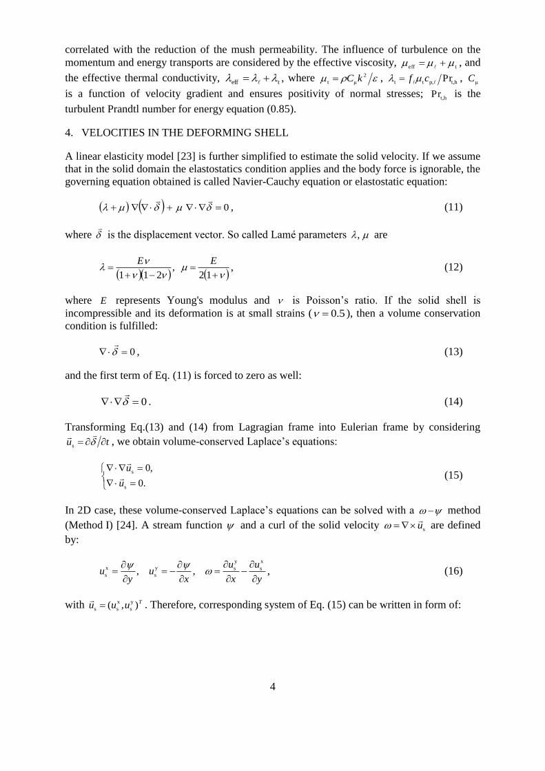
improve the accuracy a necessity to use separate refinement regions for the temperature and

solid fraction fields was approved previously by authors [5]. Thereby based on the error

analysis of the energy equation and the resolution criterion of the Gulliver-Scheil correlation

(Eq.(1)), consecutive mesh refinements were made (Figure 9). Eventually mesh independent

results were obtained.

Figure 9. Mesh refinement to track the temperature boundary layer and solidification front

c)

Figure 10. Quasi steady state simulation result of an engineering TSC. a) 3D distribution of

the velocity vector field and evolution of the solid shell (dark region in the 5 cross sections);

b) zoomed velocity field in the central plane near the narrow face; c) detailed velocity

(uy component) profile and solid volume fraction along two paths cross the mushy zone.

Based on the aforementioned model a simulation of the real engineering TSC (width 1726

mm and thickness 72 mm) was performed, and the calculation result is shown in Figure 10.

The calculation domain includes the submerge entry nozzle and entire mold region and part of

water cooled strand (till 2000 mm from meniscus). To ensure the calculation accuracy

numerical techniques like parallel computing and mesh adaptation are necessarily applied.

More than 1 million computational cells are used to resolve the interdendritic flow in the

u

(m/s)

a) b)

temperature

boundary

layer

mushy zone

boundary

layer

Mold

w

all

Bulk

liq

uid

12

mushy zone (Figure 10(c)). In [2,3] Laplace’s equation was solved for solid velocities with a

constant vertical component assumption restricting longitudinal deformations. The new

approach doesn’t have such a limitation and helps to mimic the mush better.

7. MODELING DISCRETE PHASE

Based on the implementation of the DPM solver in the OpenFOAM CFD software package, a

number of simulations were made.

First of all, comparison of the nonmetallic inclusion and gas bubbles behavior in the turbulent

flow was made (Figure 11). Particles of two types (with densities of 2700 and 5000 kg/m3

accordingly) and argon bubbles (density 0.19 kg/m3) were injected from different points of

the 2D continuous casting mold geometry with the steady state fluid flow been established. It

is marked on the figures by the gray-colored stream lines.

Figure 11: Initial injection of the particles and gas bubbles

Bubbles (blue circles) and particles (red dots), presented at the left draw, were ejected through

SEN with the same initial velocities. On the right picture, black-dotted particles are injected at

the region of the large top vortex at the slag region, other (red and green) at the SEN ports.

The only difference in the simulation setup for green-marked particles is that

turbulence / particle interaction is not taken into account (in other word, DRW model is

switched off for that type of objects). Hereby it is possible to estimate the significance of the

eddy influence on the particle trajectories.

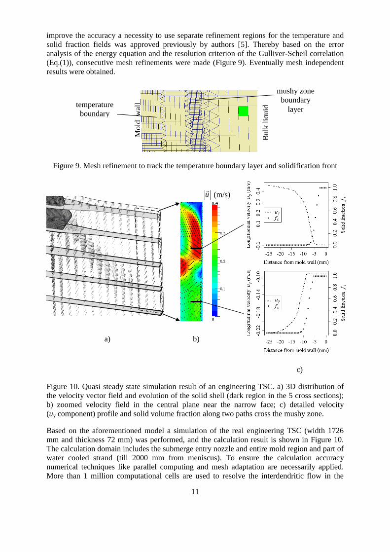
Further one can see (Figure 12) how the distribution of the gas bubbles and particles

dramatically changes after they are involved by the flow. Bubbles, as it was emphasized here

before, are strongly influenced by the buoyancy force counteracting the main flow drag: even

at the initial stages of the simulation some of the gas bubbles are already captured by the slag.

Smaller particles mostly follow the melt motion. Additionally, they are spread out over the

simulation domain due to the interaction with the turbulent flow.

13

Figure 12: Gas bubbles and solid particles distribution after injection is complete

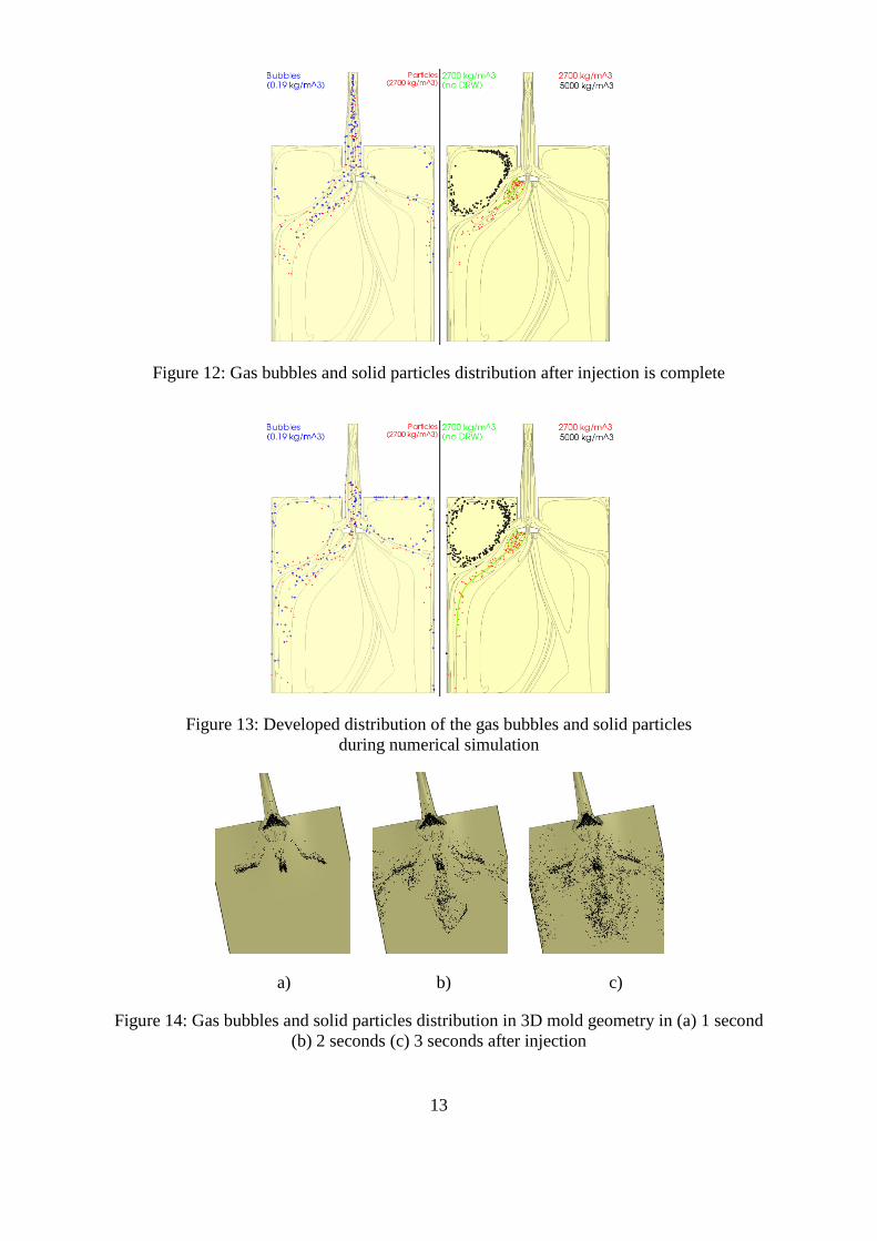
Figure 13: Developed distribution of the gas bubbles and solid particles

during numerical simulation

a) b) c)

Figure 14: Gas bubbles and solid particles distribution in 3D mold geometry in (a) 1 second

(b) 2 seconds (c) 3 seconds after injection

14

Finally, after the motion of the particles and bubbles is developing in the course of time

(Figure 13), following conclusions can be made: gas bubbles mostly tend to rise to the slag

surface; however some of them are still brought with the melt flow downwards and leave the

simulation domain through the outlet; thereby they can be entrapped into the final product and

facilitate the porosity formation; particle inclusions are strongly influenced by the melt flow;

turbulence dramatically enhances their distribution (e.g. green colored particles strictly follow

the stream lines as opposed to other types with the DRW model taken into account).

Dispersion effect is even more amplified in 3D real geometries (Figure 14).

Obtained results emphasize the importance of the flow pattern in the continuous casting mold,

which can either enhance or reduce the porosity formation and nonmetallic inclusions

entrapment into final product.

Presented analysis of the results, obtained with the developed solver for the simulation of the

nonmetallic inclusions and the gas bubbles in the continuous casting mold, sustains the

efficiency of the numerical experiment concept for the continuous casting especially when it

is rather difficult to receive measurement’s and experimental data. Open-source CFD package

OpenFOAM proved to be an excellent design tool for the implementation and further

development of the DPM approach for the multiphase flows simulation.

8. VERIFICATION OF THE DPM MODEL

As an extension of the presented work a verification of the DPM solver was carried out based

on the obtained results of the water modeling experiment regarding the particle flow.

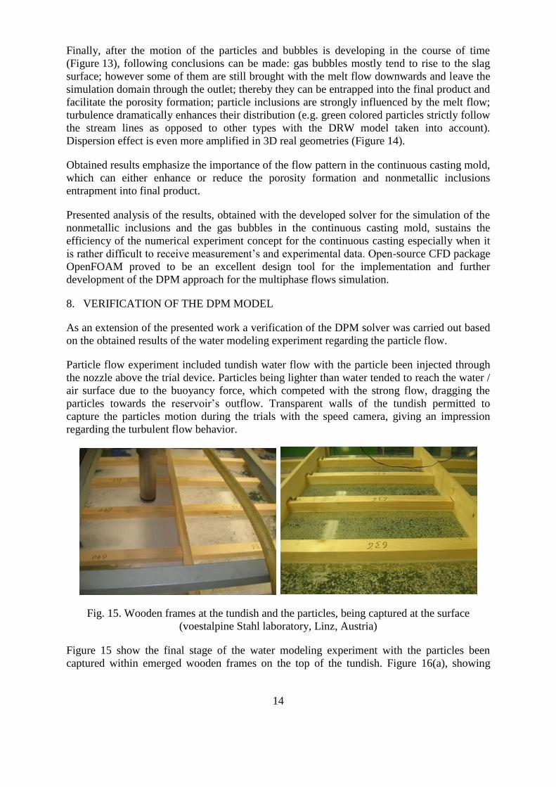
Particle flow experiment included tundish water flow with the particle been injected through

the nozzle above the trial device. Particles being lighter than water tended to reach the water /

air surface due to the buoyancy force, which competed with the strong flow, dragging the

particles towards the reservoir’s outflow. Transparent walls of the tundish permitted to

capture the particles motion during the trials with the speed camera, giving an impression

regarding the turbulent flow behavior.

Fig. 15. Wooden frames at the tundish and the particles, being captured at the surface

(voestalpine Stahl laboratory, Linz, Austria)

Figure 15 show the final stage of the water modeling experiment with the particles been

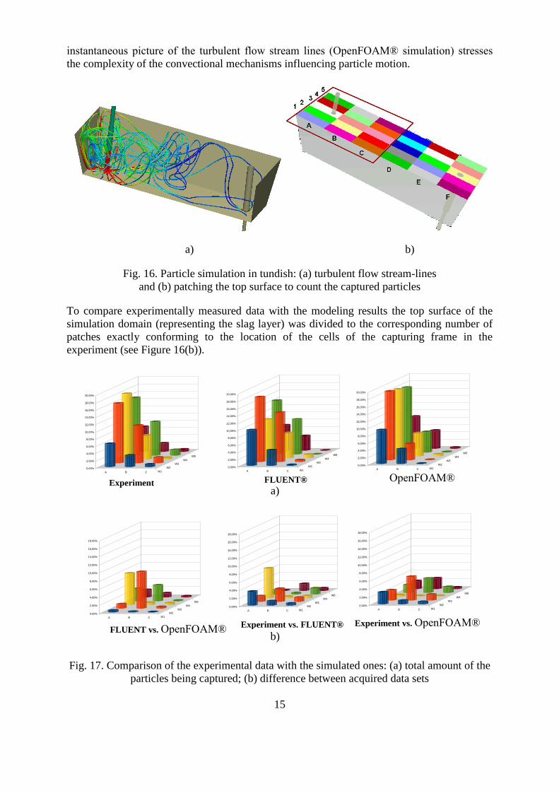
captured within emerged wooden frames on the top of the tundish. Figure 16(a), showing

15

instantaneous picture of the turbulent flow stream lines (OpenFOAM® simulation) stresses

the complexity of the convectional mechanisms influencing particle motion.

a) b)

Fig. 16. Particle simulation in tundish: (a) turbulent flow stream-lines

and (b) patching the top surface to count the captured particles

To compare experimentally measured data with the modeling results the top surface of the

simulation domain (representing the slag layer) was divided to the corresponding number of

patches exactly conforming to the location of the cells of the capturing frame in the

experiment (see Figure 16(b)).

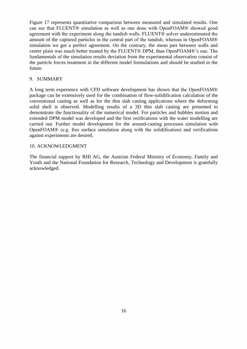
Fig. 17. Comparison of the experimental data with the simulated ones: (a) total amount of the

particles being captured; (b) difference between acquired data sets

0,00%

2,00%

4,00%

6,00%

8,00%

10,00%

12,00%

14,00%

16,00%

18,00%

A B C W1

W2

W3

W4

W5

0,00%

2,00%

4,00%

6,00%

8,00%

10,00%

12,00%

14,00%

16,00%

18,00%

A B C W1

W2

W3

W4

W5

0,00%

2,00%

4,00%

6,00%

8,00%

10,00%

12,00%

14,00%

16,00%

18,00%

20,00%

A B C W1

W2

W3

W4

W5

0,00%

2,00%

4,00%

6,00%

8,00%

10,00%

12,00%

14,00%

16,00%

18,00%

20,00%

A B C W1

W2

W3

W4

W5

0,00%

2,00%

4,00%

6,00%

8,00%

10,00%

12,00%

14,00%

16,00%

18,00%

20,00%

A B C W1

W2

W3

W4

W5

a)

b)

0,00%

2,00%

4,00%

6,00%

8,00%

10,00%

12,00%

14,00%

16,00%

18,00%

A B C W1

W2

W3

W4

W5

Experiment FLUENT® OpenFOAM®

FLUENT vs. OpenFOAM® Experiment vs. FLUENT® Experiment vs. OpenFOAM®

16

Figure 17 represents quantitative comparison between measured and simulated results. One

can see that FLUENT® simulation as well as one done with OpenFOAM® showed good

agreement with the experiment along the tundish walls. FLUENT® solver underestimated the

amount of the captured particles in the central part of the tundish, whereas in OpenFOAM®

simulation we got a perfect agreement. On the contrary, the mean part between walls and

center plain was much better treated by the FLUENT® DPM, than OpenFOAM®’s one. The

fundamentals of the simulation results deviation from the experimental observation consist of

the particle forces treatment in the different model formulations and should be studied in the

future.

9. SUMMARY

A long term experience with CFD software development has shown that the OpenFOAM®

package can be extensively used for the combination of flow-solidification calculation of the

conventional casting as well as for the thin slab casting applications where the deforming

solid shell is observed. Modelling results of a 3D thin slab casting are presented to

demonstrate the functionality of the numerical model. For particles and bubbles motion and

extended DPM model was developed and the first verifications with the water modelling are

carried out. Further model development for the around-casting processes simulation with

OpenFOAM® (e.g. free surface simulation along with the solidification) and verifications

against experiments are desired.

10. ACKNOWLEDGMENT

The financial support by RHI AG, the Austrian Federal Ministry of Economy, Family and

Youth and the National Foundation for Research, Technology and Development is gratefully

acknowledged.

17

REFERENCES

[1] M. Wu, A. Vakhrushev, G. Nummer, C. Pfeiler, A. Kharicha and A. Ludwig, Importance

of Melt Flow in Solidifying Mushy Zone. Open Transport Phenomena J. – Bentham Open. 2,

pp. 16-23 (2010)

[2] A. Vakhrushev, A. Ludwig, M. Wu, Y. Tang, G. Nitzl and G. Hackl, Modeling of

Turbulent Melt Flow and Solidification Processes in Steel Continuous Caster with the Open

Source Software Package OpenFOAM®. Proc. OSCIC’10, Munich, Nov. 4-5, pp. 1-17 (2010)

[3] A. Vakhrushev, A. Ludwig, M. Wu, Y. Tang, G. Nitzl and G. Hackl, Modeling of Heat

Transfer and Solidification Processes in Thin Slab Caster. Proc. ECCC 2011, Düsseldorf,

June 27 – July 01, S18, pp. 1-10 (2011)

[4] A. Vakhrushev, A. Ludwig, M. Wu, Y. Tang, G. Nitzl and G. Hackl, Modeling of

nonmetallic inclusions and gas bubbles motion in continuous caster. Proc. STEELSIM 2011,

Düsseldorf, June 27 – July 01, S17, pp. 1-8 (2011)

[5] A. Vakhrushev, A. Ludwig, M. Wu, Y. Tang, G. Nitzl and G. Hackl, Coupling the

turbulent flow with the solidification processes in OpenFOAM®. Proc. OSCIC’11, Paris

Chantilly, Nov. 3-4, pp. 1-21 (2011)

[6] Prescott PJ and Incropera FP 1994 Transp. Phen. in Mater. Proc. & Manuf.- ASME HTD

280 59.

[7] Prescott PJ and Incropera FP 1994 J. Heat Transfer 116 735.

[8] Prescott PJ, Incropera FP and Gaskell DR 1994 Trans. ASME 116 742.

[9] Prescott PJ and Incropera FP 1995 Trans. ASME 117 716.

[10] Pfeiler C, Thomas BG, Wu M, Ludwig A and Kharicha A 2008 Steel Res. Int. 79 599.

[11] Voller VR and Prakash C 1987 Int. J. Heat Mass Transfer 30 1709.

[12] Voller VR, Brent AD and Prakash C 1989 Int. J. Heat Mass Transfer 32 1719.

[13] Voller VR, Brent AD and Prakash C 1990 Appl. Math. Modeling 14 320.

[14] Chakraborty PR and Dutta P 2011 Metall. Mater. Trans. 42B in press (DOI:

10.1007/s11663-011-9585-3).

[15] Yin RY 2009 J. Iron & Steel Res. 16 (Supplement 1) 1.

[16] Birat JP and Bobadilla M 2006 Proc. McWASP XI (Eds: Gandin CA and Bellet M,

TMS Publications) 33.

[17] Tang Y, Krobath M, Nitzl G, Eglsaeer C and Morales R 2009 J. Iron & Steel Res. 16

(Supplement 1) 173.

18

[18] Thomas BG 2001 Brimacombe Lecture, 59th

Electric Furnace Conf. (Iron & Steel

Soc.) 3.

[19] Tian X, Zou F, Li B and He J 2010 Metall. Mater. Trans. 41B 112

[20] Graham, D. I.; James, P. W.: Turbulent dispersion of particles using eddy interaction

models; Int. J. Multiphase Flow, 1996, vol. 22, Issue 1, P. 157-175

[21] Graham, D. I.: On the inertia effect in eddy interaction models; Int. J. Multiphase Flow,

1996, vol. 22, Issue 1, P. 177-184

[22] Gu JP and Beckermann C 1999 Metall. Mater. Trans. 33A 1357.

[23] Slaughter WS 2002 The Linearized Theory of Elasticity (Boston: Birkhäuser).

[24]Roache PJ 1998 Fundamentals of Computational Fluid Dynamics (New Mexico:

Hermosa Publishers)

[25] Rhie, C. M.; Chow, W. L.: A numerical study of the turbulent flow past an isolated

airfoil with trailing edge separation; 3rd Joint Thermophysics, Fluids, Plasma and Heat

Transfer Conference, St. Louis, Missouri, 1982

[26] Perić, M.: A Finite Volume method for the prediction of three-dimensional fluid flow in

complex ducts; PhD thesis, Imperial College, University of London, 1985