Embed Size (px)
Citation preview

UNIVERSITY OF SOUTHAMPTON
FACULTY OF ENGINEERING AND THE ENVIRONMENT
Institute of Sound and Vibration Research
Advanced Open Rotor Far-Field Tone Noise
by
Celia Maud Ekoule
PhD thesis
April 2017


ABSTRACT
Doctor of Philosophy
ADVANCED OPEN ROTOR FAR-FIELD TONE NOISE
by Celia Maud Ekoule
An extensive analysis of the far-field tonal noise produced by an advanced open
rotor is presented. The basis of the work is analytical methods which have been
developed to predict the tonal noise generated by several different mechanisms.
Also to provide further insight and validation, an in-depth analysis of rig-scale
wind tunnel measurements and Computational Fluid Dynamics (CFD) data has
been carried out.
The loading noise produced by a propeller operating at angle of attack is for-
mulated modeling the blades as a cascade of a two-dimensional flat plates. The
simplified geometry enables the prediction of rotor-alone tones with a reduced com-
puter processing time. The method shows a good ability to predict the relative
change of the sound pressure level with changes of the angle of attack.
The radiated sound field caused by aerodynamic interactions between the two
blade rows is investigated. A hybrid analytical/computational method is devel-
oped to predict the tonal noise produced by the interaction between the front
rotor viscous wakes and the rear rotor. The method assumes a Gaussian wake
profile whose characteristics are determined numerically in the inter-rotor region
and propagated analytically to the downstream blade row. A cross validation of
the prediction method against wind tunnel measurements and CFD data shows
reasonable agreement between the three techniques for a wide number of interac-
tion tones.
Additionally a theoretical formulation is derived for expressions for the tonal noise
generated by the interaction between the bound potential field of one rotor with
the adjacent rotor. The bound potential field produced by the thickness and bound
circulation of each blade is determined using a distributed source model. The ana-
lytical model is compared with an existing model for a point source and is validated
using advanced CFD computations. Results show that the potential field mostly
affects the first interaction tone. The addition of the potential field component
provides an improvement in the agreement with wind tunnel measurements.
Overall this work provides new tools for the rapid assessment of the tonal noise
produced by an advance open rotor at various operating conditions, and the ana-
lytical result can provide further physical insight into the sources of noise.

iv

Contents
Declaration of Authorship xiii
Acknowledgements xv
Nomenclature 1
1 Introduction 5
1.1 Background . . . . . . . . . . . . . . . . . . . . . . . . . . . . . . . 5
1.2 Single-rotating open rotor . . . . . . . . . . . . . . . . . . . . . . . 8
1.3 Contra-rotating open rotor or Advanced Open Rotor (AOR) . . . . 10
1.4 Installation effects . . . . . . . . . . . . . . . . . . . . . . . . . . . . 13
1.4.1 Angle of attack . . . . . . . . . . . . . . . . . . . . . . . . . 13
1.4.2 Fuselage scattering . . . . . . . . . . . . . . . . . . . . . . . 15
1.4.3 Wing and pylon . . . . . . . . . . . . . . . . . . . . . . . . . 17
1.5 Aims, objectives and original contributions . . . . . . . . . . . . . . 19
2 Model scale open rotor data analysis 21
2.1 Description of the wind tunnel facility . . . . . . . . . . . . . . . . 21
2.1.1 Rig 145 Build 2 test campaign . . . . . . . . . . . . . . . . . 22
2.1.2 Z08 rig test campaign . . . . . . . . . . . . . . . . . . . . . 24
2.2 Acoustic data processing . . . . . . . . . . . . . . . . . . . . . . . . 27
2.2.1 Emission and reception coordinate systems . . . . . . . . . . 27
2.2.2 Post-processing methods . . . . . . . . . . . . . . . . . . . . 29
2.3 Measurement issues . . . . . . . . . . . . . . . . . . . . . . . . . . . 33
2.3.1 Haystacking . . . . . . . . . . . . . . . . . . . . . . . . . . . 33
2.3.2 Measurements uncertainties . . . . . . . . . . . . . . . . . . 35
2.4 Results . . . . . . . . . . . . . . . . . . . . . . . . . . . . . . . . . . 37
2.4.1 Rig 145 tests . . . . . . . . . . . . . . . . . . . . . . . . . . 37
2.4.2 Z08 rig tests . . . . . . . . . . . . . . . . . . . . . . . . . . . 46
2.5 Concluding remarks . . . . . . . . . . . . . . . . . . . . . . . . . . . 49
3 Loading noise produced by a single rotor at angle of attack 51
3.1 Steady loading . . . . . . . . . . . . . . . . . . . . . . . . . . . . . 51
3.2 Unsteady loading due to angle of attack . . . . . . . . . . . . . . . 61
3.3 Results . . . . . . . . . . . . . . . . . . . . . . . . . . . . . . . . . . 66
3.4 Concluding remarks . . . . . . . . . . . . . . . . . . . . . . . . . . . 66
v

vi CONTENTS
4 Interaction tone prediction 67
4.1 Downstream interactions . . . . . . . . . . . . . . . . . . . . . . . . 68
4.2 Upstream interactions . . . . . . . . . . . . . . . . . . . . . . . . . 75
4.3 Concluding remarks . . . . . . . . . . . . . . . . . . . . . . . . . . . 76
5 Wake interaction noise 77
5.1 Introduction . . . . . . . . . . . . . . . . . . . . . . . . . . . . . . . 77
5.2 Hybrid CFD/analytical model . . . . . . . . . . . . . . . . . . . . . 78
5.2.1 Method . . . . . . . . . . . . . . . . . . . . . . . . . . . . . 78
5.2.2 Coordinate system . . . . . . . . . . . . . . . . . . . . . . . 80
5.2.3 Wake velocity profile . . . . . . . . . . . . . . . . . . . . . . 81
5.2.4 Airfoil response . . . . . . . . . . . . . . . . . . . . . . . . . 92
5.3 Wake interaction noise prediction . . . . . . . . . . . . . . . . . . . 99
5.4 Concluding remarks . . . . . . . . . . . . . . . . . . . . . . . . . . . 105
6 Potential field interactions 107
6.1 Introduction . . . . . . . . . . . . . . . . . . . . . . . . . . . . . . . 107
6.2 Upstream interactions . . . . . . . . . . . . . . . . . . . . . . . . . 109
6.2.1 Potential field due to blade thickness . . . . . . . . . . . . . 110
6.2.2 Potential field due to blade circulation . . . . . . . . . . . . 127
6.2.3 Response of the upstream airfoil . . . . . . . . . . . . . . . . 136
6.3 Downstream interactions . . . . . . . . . . . . . . . . . . . . . . . . 141
6.3.1 Potential field due to blade thickness . . . . . . . . . . . . . 142
6.3.2 Potential field due to blade circulation . . . . . . . . . . . . 149
6.3.3 Response of the downstream airfoil . . . . . . . . . . . . . . 150
6.4 Potential field interaction noise prediction . . . . . . . . . . . . . . 153
6.5 Concluding remarks . . . . . . . . . . . . . . . . . . . . . . . . . . . 157
7 Conclusions 159
7.1 Research outcomes . . . . . . . . . . . . . . . . . . . . . . . . . . . 159
7.2 Further research . . . . . . . . . . . . . . . . . . . . . . . . . . . . . 162
A Evaluation of Ix and Iφ 163
B Coordinate systems 165
C Profile drag and β 169
D Parry’s method for the potential field interactions prediction 175
D.1 Potential due to blade thickness for an elliptic airfoil . . . . . . . . 175
D.2 Potential due to blade circulation . . . . . . . . . . . . . . . . . . . 179
D.3 Simplification of the distributed source model for an ellipse . . . . . 179
References 181

List of Figures
1.1 Evolution of world annual traffic in Revenue Passenger Kilometres(RPK) from 1970 to 2012, source: Airbus (2013). . . . . . . . . . . 6
1.2 Cut-away view of an advanced open rotor concept (picture courtesyof Rolls-Royce plc.) . . . . . . . . . . . . . . . . . . . . . . . . . . . 6
1.3 Relative SFC and EPNL noise reduction for Turbofan of the year2000, Open Rotor and Advanced Turbofan (picture courtesy ofRolls-Royce plc.) . . . . . . . . . . . . . . . . . . . . . . . . . . . . 7
1.4 Sources of AOR tonal noise. . . . . . . . . . . . . . . . . . . . . . . 11
1.5 Definition of the angle of attack. . . . . . . . . . . . . . . . . . . . . 14
2.1 Schematic showing the experimental test set-up during testing ofRig 145 Build 2 in the DNW wind tunnel. Published in Parry et al.(2011). . . . . . . . . . . . . . . . . . . . . . . . . . . . . . . . . . . 22
2.2 Rig145 Build 2 installed in the DNW wind tunnel. Published inParry et al. (2011). . . . . . . . . . . . . . . . . . . . . . . . . . . . 23
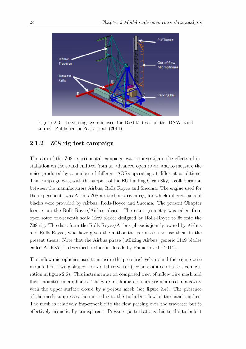
2.3 Traversing system used for Rig145 tests in the DNW wind tunnel.Published in Parry et al. (2011). . . . . . . . . . . . . . . . . . . . . 24
2.4 Sketch of a wire-mesh microphone mounted on an airfoil. . . . . . 25
2.5 Sketch of a flush-mounted microphone on an airfoil. . . . . . . . . 25
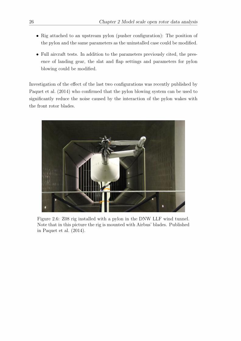
2.6 Z08 rig installed with a pylon in the DNW LLF wind tunnel. Notethat in this picture the rig is mounted with Airbus’ blades. Pub-lished in Paquet et al. (2014). . . . . . . . . . . . . . . . . . . . . . 26
2.7 Emission and reception coordinates for the flyover (a) and windtunnel (b) testing cases. . . . . . . . . . . . . . . . . . . . . . . . . 28
2.8 Background noise correction. . . . . . . . . . . . . . . . . . . . . . . 30
2.9 Broadband noise calculation. . . . . . . . . . . . . . . . . . . . . . . 30
2.10 Tones identification. . . . . . . . . . . . . . . . . . . . . . . . . . . 31
2.11 Broadband noise correction. . . . . . . . . . . . . . . . . . . . . . . 31
2.12 Tones unbroadening. . . . . . . . . . . . . . . . . . . . . . . . . . . 32
2.13 Scattering effects in a wind tunnel. . . . . . . . . . . . . . . . . . . 33
2.14 Narrow band SPL spectrum at 90 of an inflow and an out-of-flowmicrophone at the same take-off case - Rig 145 tests. . . . . . . . . 34
2.15 Microphone set-up on the Rig 145 inflow traversing system (source:Parry et al. (2011)). . . . . . . . . . . . . . . . . . . . . . . . . . . . 35
vii

viii LIST OF FIGURES
2.16 Polar directivity pattern of the first front rotor alone tone mea-sured at a typical takeoff case by a selection of inflow traversingmicrophones and at a given emission radius - Rig 145. . . . . . . . . 36
2.17 Polar directivity of the first rotor alone tone measured by the inflowmicrophones at a typical take-off case - Rig 145 build 2. . . . . . . . 36
2.18 A typical spectrum with tones annotations for a particular take-offcase . . . . . . . . . . . . . . . . . . . . . . . . . . . . . . . . . . . 37
2.19 Polar directivity of the tone 1, 0 at typical take-off, approach andcut-back conditions - Rig 145. . . . . . . . . . . . . . . . . . . . . . 38
2.20 Polar directivity of the tone 1, 1 at typical take-off, approach andcut-back conditions - Rig 145. . . . . . . . . . . . . . . . . . . . . . 39
2.21 Polar directivity of the tone 1, 2 at typical take-off, approach andcut-back conditions - Rig 145. . . . . . . . . . . . . . . . . . . . . . 39
2.22 Polar directivity of the 1, 0 tone at take-off at different rotationalspeed settings - Rig 145. . . . . . . . . . . . . . . . . . . . . . . . . 40
2.23 Polar directivity of the 1, 1 tone at take-off at different rotationalspeed settings - Rig 145. . . . . . . . . . . . . . . . . . . . . . . . . 40
2.24 Polar directivity of the 1, 2 tone at take-off at different rotationalspeed settings - Rig 145. . . . . . . . . . . . . . . . . . . . . . . . . 41
2.25 Broadband and tones contributions in a typical AOR frequencyspectrum. . . . . . . . . . . . . . . . . . . . . . . . . . . . . . . . . 42
2.26 One-third octave band spectra at 90 degrees (take-off). . . . . . . . 43
2.27 One-third octave band spectrum at 90 degrees (cutback). . . . . . . 43
2.28 One-third octave band spectrum at 90 degrees (approach). . . . . . 44
2.29 One third octave band spectra at various polar angles (take-off). . . 44
2.30 Comparison with predictions - rig145. . . . . . . . . . . . . . . . . . 45
2.31 Comparison with predictions - rig145. . . . . . . . . . . . . . . . . . 46
2.32 Polar directivity of the 1, 0 tone at take-off measured by wiremeshmicrophones - Z08. . . . . . . . . . . . . . . . . . . . . . . . . . . . 47
2.33 Polar directivity of the 1, 1 interaction tone at take-off measuredby wiremesh microphones - Z08. . . . . . . . . . . . . . . . . . . . . 47
2.34 Polar directivity of the 1, 2 interaction tone at take-off measuredby wiremesh microphones - Z08. . . . . . . . . . . . . . . . . . . . . 48
2.35 One-third octave band spectra at 90 measured by wire-mesh mi-crophones (take-off). . . . . . . . . . . . . . . . . . . . . . . . . . . 48
3.1 Source coordinates in flight and propeller system. . . . . . . . . . . 53
3.2 Flat blade approximation. . . . . . . . . . . . . . . . . . . . . . . . 54
3.3 Emission and reception coordinate systems for an AOR at angle ofattack (flyover case). . . . . . . . . . . . . . . . . . . . . . . . . . . 58
3.4 Flight and propeller coordinates. . . . . . . . . . . . . . . . . . . . 62
3.5 Blade coordinates system. . . . . . . . . . . . . . . . . . . . . . . . 62
3.6 Coordinates system for velocity components. . . . . . . . . . . . . . 63

LIST OF FIGURES ix
3.7 Polar directivity of the first rotor-alone tone for Rig 145 operating ata condition representative of take-off (φ′ = 0). Measured SPL(left)predicted SPL (right). . . . . . . . . . . . . . . . . . . . . . . . . . 66
4.1 Cascade representation of the front and rear rotor blades at constantradius ry. . . . . . . . . . . . . . . . . . . . . . . . . . . . . . . . . 68
4.2 Blade sweep and lean definition. . . . . . . . . . . . . . . . . . . . . 74
5.1 Blade-to-blade mesh topology, originally published by Sohoni et al.(2015). S and ε correspond to pitch and thickness quantities. . . . . 79
5.2 Contours of constant instantaneous velocity in a meridional plane:(a) axial velocity, (b), radial velocity. The color scaling limit Vmaxcorresponds to the maximum absolute velocity magnitude acrossthe meridional plane and Vmin ≈ −0.7Vmax. . . . . . . . . . . . . . . 79
5.3 Cascade coordinate system. . . . . . . . . . . . . . . . . . . . . . . 80
5.4 Location of the plane P1. . . . . . . . . . . . . . . . . . . . . . . . . 81
5.5 Contours of constant tangential velocity (normalized by the maxi-mum tangential velocity) at x/D = 0.0902 downstream of the frontrotor blade pitch change axis for one blade passage. . . . . . . . . . 82
5.6 Plot of normalized tangential velocity versus φ1 at r = 0.8Rt1 ,x/D1 = 0.0902 downstream of the front rotor blade pitch change axis. 82
5.7 Normalized wake velocity deficit at radius r = 0.8Rt1 . Comparisonbetween the analytical model and the CFD data at the measurementplane. . . . . . . . . . . . . . . . . . . . . . . . . . . . . . . . . . . 83
5.8 Tangential velocity at the plane P1 normalized by the front rotortip speed given by the CFD data (a) and the analytical model (b). . 84
5.9 Evolution of the wake velocity deficit uc between the two rotors atr = 60%Rt1 . . . . . . . . . . . . . . . . . . . . . . . . . . . . . . . . 85
5.10 Evolution of β (m−2) between the two rotors at r = 60%Rt1 . . . . . 86
5.11 Location of the plane P2. . . . . . . . . . . . . . . . . . . . . . . . . 86
5.12 Normalized wake deficit, at a distance 0.144D1 downstream of thefront rotor pitch change axis calculated by (a) fitting a Gaussianprofile to the CFD data in this plane, (b) using the data collectedat the original measurement plane and propagating the wakes down-stream using the scaling laws (5.5) and (5.6). . . . . . . . . . . . . . 87
5.13 Normalized wake velocity deficit at the plane P2 at r ≈ 0.8Rt1 . Theterm Ur1 is the mean velocity magnitude at this location. . . . . . . 88
5.14 Normalized upwash velocity at the rear rotor inlet plane (r ≈0.8Rt1): (a) velocity magnitude, (b) Fourier harmonics. . . . . . . . 91
5.15 Airfoil response for k = 1. (a) predicted levels, (b) numerical results. 95
5.16 Airfoil response for k = 2. (a) predicted levels, (b) numerical results. 96
5.17 Airfoil response for k = 3. (a) predicted levels, (b) numerical results. 97
5.18 Lift per unit span for (a) k = 1, (b) k = 2, (c) k = 3. . . . . . . . . 98
5.19 SPL spectrum for an isolated open rotor rig operating at a take-off type thrust measured at a polar emission angle θ′ = 90 andnormalized to a constant emission radius. . . . . . . . . . . . . . . 100

x LIST OF FIGURES
5.20 Sonic radius plotted against frequency at a polar emission angleθ′ = 90 for each of the interaction tones expected to occur atfrequencies ω for the given take-off case. Tones are labelled n1, n2. 100
5.21 Polar directivity of the tone 1, 1 for a given take-off case comparedwith wind tunnel measurements and CFD data. . . . . . . . . . . . 102
5.22 Polar directivity of the tone 1, 2 for a given take-off case comparedwith wind tunnel measurements and CFD data. . . . . . . . . . . . 102
5.23 Polar directivity of the tone 2, 2 for a given take-off case comparedwith wind tunnel measurements and CFD data. . . . . . . . . . . . 103
5.24 Polar directivity of the tone 3, 4 for a given take-off case comparedwith wind tunnel measurements and CFD data. . . . . . . . . . . . 103
5.25 Polar directivity of the tone 3, 6 for a given take-off case comparedwith wind tunnel measurements and CFD data. . . . . . . . . . . . 104
5.26 Polar directivity of the tone 4, 4 for a given take-off case comparedwith wind tunnel measurements and CFD data. . . . . . . . . . . . 104
6.1 Airfoil geometry. . . . . . . . . . . . . . . . . . . . . . . . . . . . . 109
6.2 Coordinate system for the interaction of the downstream potentialfield with the upstream row. . . . . . . . . . . . . . . . . . . . . . . 110
6.3 Thickness source distribution. . . . . . . . . . . . . . . . . . . . . . 112
6.4 Velocity potential calculated with model 1. . . . . . . . . . . . . . . 113
6.5 Upwash velocity (normalized against the free stream velocity) cal-culated using models 1 and 2 at r = 60%Rt1 . Geometry A: sum ofsine functions; Geometry B: ellipse. . . . . . . . . . . . . . . . . . . 114
6.6 Percentage difference in upwash velocity between model 1 (withgeometry A) and model 2. . . . . . . . . . . . . . . . . . . . . . . . 115
6.7 Percentage difference in upwash velocity between model 1 (using anelliptic geometry) and model 2. . . . . . . . . . . . . . . . . . . . . 115
6.8 Thickness source cascade distribution. . . . . . . . . . . . . . . . . . 118
6.9 Contour integration. . . . . . . . . . . . . . . . . . . . . . . . . . . 119
6.10 Magnitude of the first ten harmonics of the upwash velocity nor-malized by the free stream velocity at the upstream blade’s trailingedge at r ≈ 60%Rt1 . Geometry A: sum of sine functions; GeometryB: ellipse. . . . . . . . . . . . . . . . . . . . . . . . . . . . . . . . . 123
6.11 Amplitude of the first upwash harmonic (normalized against thefree stream velocity U∞) at the upstream blade’s trailing edge. Ge-ometry A:sum of sine functions; Geometry B: ellipse. . . . . . . . . 124
6.12 Amplitude of the fifth upwash harmonic (normalized against thefree stream velocity U∞) at the upstream blade’s trailing edge. Ge-ometry A: sum of sine functions; Geometry B: ellipse. . . . . . . . . 125
6.13 Amplitude of the first upwash harmonic (normalized against the freestream velocity U∞) calculated by model 1 at the upstream blade’strailing edge at r ≈ 60%Rt1 . Geometry A: sum of sine functions;Geometry B: ellipse; Geometry C: combination of a sine functionand an ellipse. . . . . . . . . . . . . . . . . . . . . . . . . . . . . . . 126

LIST OF FIGURES xi
6.14 Amplitude of the fifth upwash harmonic (normalized against thefree stream velocity U∞) calculated by model 1 at the upstreamblade’s trailing edge at r ≈ 60%Rt1 . Geometry A: sum of sinefunctions; Geometry B: ellipse; Geometry C: combination of a sinefunction and an ellipse. . . . . . . . . . . . . . . . . . . . . . . . . . 127
6.15 Vortex source distribution. . . . . . . . . . . . . . . . . . . . . . . . 129
6.16 Upwash velocity magnitude normalized against the free stream ve-locity U∞ at r ≈ 60%Rt1 . . . . . . . . . . . . . . . . . . . . . . . . . 132
6.17 Amplitude of the first upwash harmonic normalized against the freestream velocity U∞ at the front rotor trailing edge. . . . . . . . . . 132
6.18 Amplitude of the first upwash harmonic normalized against the freestream velocity U∞ in the inter-rotor region. The analytical modelsare compared with the CFD data. . . . . . . . . . . . . . . . . . . . 133
6.19 Upwash velocity captured by the CFD one cell upstream and down-stream of the sliding plane for one rear rotor’s blade passage. . . . . 134
6.20 Axial component of the downstream airfoil’s velocity potential nor-malized against the free-stream velocity captured by the CFD atr ≈ 60%Rt1 in the inter-rotor region. . . . . . . . . . . . . . . . . . 135
6.21 Upwash velocity normalized against the free-stream velocity cap-tured by the CFD at r ≈ 60%Rt1 in the inter-rotor region. . . . . . 135
6.22 First harmonic of the lift per unit span acting on the upstream blade.138
6.23 Fifth harmonic of the lift per unit span acting on the upstream blade.139
6.24 Comparison between the first harmonic of the lift per unit spanacting on the upstream blade provided by the analytical modelsand the CFD. . . . . . . . . . . . . . . . . . . . . . . . . . . . . . . 140
6.25 Amplitude of the first three upwash harmonics determined from theCFD data. . . . . . . . . . . . . . . . . . . . . . . . . . . . . . . . . 140
6.26 Coordinate system for the interaction of the upstream potential fieldwith the downstream row. . . . . . . . . . . . . . . . . . . . . . . . 141
6.27 Thickness source cascade distribution. . . . . . . . . . . . . . . . . . 144
6.28 Contour integration. . . . . . . . . . . . . . . . . . . . . . . . . . . 145
6.29 Amplitude of the first upwash harmonic normalized against the freestream velocity at the downstream blade’s leading edge (thicknesscontribution). . . . . . . . . . . . . . . . . . . . . . . . . . . . . . 148
6.30 Amplitude of the fifth upwash harmonic normalized against the freestream velocity at the downstream blade’s leading edge (thicknesscontribution). . . . . . . . . . . . . . . . . . . . . . . . . . . . . . 148
6.31 Amplitude of the first upwash harmonic (loading contribution) nor-malized against the free stream velocity at the downstream blade’sleading edge. . . . . . . . . . . . . . . . . . . . . . . . . . . . . . . 151
6.32 First harmonic of the lift per unit span acting on the downstreamblade. . . . . . . . . . . . . . . . . . . . . . . . . . . . . . . . . . . 152
6.33 Relative contribution of the potential field and viscous wake effectsfor the polar directivity of the tone 1, 1 compared with wind tun-nel measurements and CFD-based calculations at a given take-offcase. . . . . . . . . . . . . . . . . . . . . . . . . . . . . . . . . . . . 154
xii LIST OF FIGURES
6.34 Effect of the airfoil’s geometry on the polar directivity of the tone1, 1 caused by potential field interactions. . . . . . . . . . . . . . 154
6.35 Polar directivity of the tone 1, 1 due to the potential field in-terractions calculated using analytical models and the CFD bladeresponse. . . . . . . . . . . . . . . . . . . . . . . . . . . . . . . . . . 155
6.36 Polar directivity of the tone 1, 1 due to the potential field andwake interractions calculated using model 1 and the CFD bladeresponse compared with wind tunnel measurements. . . . . . . . . . 156
6.37 Relative contribution of the potential field and viscous wake effectsfor the polar directivity of the tone 1, 2 compared with wind tun-nel measurements and CFD-based calculations at a given take-offcase. . . . . . . . . . . . . . . . . . . . . . . . . . . . . . . . . . . . 157
C.1 Control volume around a thin airfoil at incidence angle α1 . . . . . 172
D.1 Potential field around an ellipse calculated using Milne-Thomson’smodel. . . . . . . . . . . . . . . . . . . . . . . . . . . . . . . . . . . 177
D.2 Potential field around an ellipse calculated using Parry’s model. . . 177
D.3 Comparison between Milne-Thomson and Parry’s model, in per-centage difference. . . . . . . . . . . . . . . . . . . . . . . . . . . . . 178

Declaration of Authorship
I, Celia Maud Ekoule , declare that the thesis entitled Advanced Open Rotor Far-
Field Tone Noise and the work presented in the thesis are both my own, and have
been generated by me as the result of my own original research. I confirm that:
• this work was done wholly or mainly while in candidature for a research
degree at this University;
• where any part of this thesis has previously been submitted for a degree or
any other qualification at this University or any other institution, this has
been clearly stated;
• where I have consulted the published work of others, this is always clearly
attributed;
• where I have quoted from the work of others, the source is always given.
With the exception of such quotations, this thesis is entirely my own work;
• I have acknowledged all main sources of help;
• where the thesis is based on work done by myself jointly with others, I have
made clear exactly what was done by others and what I have contributed
myself;
• parts of this work have been published as: (Kingan et al., 2014) and (Ekoule
et al., 2015)
Signed:
Date: April 21st, 2017
xiii


Acknowledgements
I would like to thank my supervisors Dr. Michael Kingan and Dr. Alan McAlpine
for their help, support, enthusiasm and constant avaibility; and my colleague Dr.
Prathiban Sureshkumar for his precious help, advice and motivation. I would like
to thank Rolls-Royce plc. for allowing me to pursue my studies and for sending
experimental data. In particular, I would like to thank Dr. Anthony Parry for
his advice, avaibility, and for the knowledge and support he provided throughout
this PhD. I would like to thank Nishad Sohoni and his colleagues for sending me
Computational Fluid Dynamics data. In addition, I gratefully acknowledge the
support of SAGE (part of the Clean Sky JTI). I would also like to thank Kimberly
Kingan for her help and support in New-Zealand, and Dr. Ana Luisa Maldonado
for her advice on key decisions during my PhD. Last but not least, I would like to
thank my close friends and family for their love and encouragement.
xv


Nomenclature
List of Symbols
Roman Letters
B = Number of propeller blades
c = Blade chord
c0 = Speed of sound in ambient fluid
CL = lift coefficient
eij = viscous stress tensor
fi = ith vector component of the surface force exerted by the air
on the blade per unit area
G = time dependent Green’s function
Gm = harmonic Green’s function
km = harmonic wave number, mB/c0
L = blade section lift
M = flight Mach number
Mt = tip rotational Mach number, (Ωrt)/c0
Mr = Mach number of the blade relative to the air
p = pressure
p0 = ambient pressure
p′ = pressure disturbance, p′ = p− p0
r = distance from propeller centre to observer
rh = blade radius at hub
rt = blade radius at tip
r′y = source radius on propeller
s = blade sweep
t = observer time
T = time limit in acoustic analogy integrals
1

2 NOMENCLATURE
T ′ij = Lighthills tensor in a moving frame
Ur = relative flow velocity
vi, v′i = velocity disturbance component in stationary fluid, in a moving
frame
Vn, V′n = source normal velocity to the blade surface in the stationary, moving
medium
X = chordwise coordinate
(x1, x2, x3) = observer (field point) coordinates
(y1, y2, y3) = source coordinates in the flight system
(y′1, y′2, y′3) = source coordinates in the propeller system
Greek Letters
α = stagger angle
αp = pitch angle of propeller shaft with respect to flight coordinate system
αy = yaw angle of propeller shaft with respect to flight coordinate system
αr = roll angle of propeller shaft with respect to flight coordinate system
β =√
1−M2
γ = angle of attack
θ, θ′ = radiation angle to observer from flight direction, propeller axis
Ω = rotational speed of propeller shaft
φ, φ′ = azimuthal angle to observer in retarded system in flight, propeller system
ΨL = noncompactness factor defined in equation 3.50
ρ = density of the fluid
ρ0 = ambient density in the undisturbed fluid
ρ′ = density disturbance, ρ− ρ0
σ = phase radius
Acronyms
AOA = Angle Of Attack
AOR = Advanced Open Rotor
BPF = Blade Passing Frequency
CFD = Computational Fluid Dynamics

3
DNW (LLF) = German-Dutch Wind Tunnels (Large Low-speed Facility)
DREAM = valiDation of Radical Engine Architecture SysteMs
ICAO = International Civil Aviation Organisation
ISVR = Institute of Sound and Vibration Research
RPM = Revolutions Per Minute
SPL = Sound Pressure Level
SROR = Single Rotating Open Rotor
URANS = Unsteady Reynolds-Averaged Navier-Stokes


Chapter 1
Introduction
1.1 Background
Improvement of the thermal and propulsive efficiency of aircraft engines has always
been a major objective of the aviation industry. Increasingly, the economic benefit
of increased global air traffic has to be balanced against the environmental impact,
driving the need for improved fuel efficiency and reduced emissions. A recent study
published in the Airbus Global Market Forecast (Airbus, 2013) showed that world-
wide annual traffic (measured in Revenue Passenger Kilometres (RPK)) increased
by 61% between 2000 and 2013 (see figure 1.1). With the continuous increase of
global air traffic, and the environmental concerns relating to global warming, air
quality and noise emissions, there is a strong incentive for aeronautical companies
to develop new aircraft engines that will reduce pollutant and noise emissions as
well as a requirement to meet the increasingly strict certification standards set by
the International Civil Aviation Organisation (ICAO).
Open rotor technology is considered as a possible alternative to turbofan engines
due to its significant improvement in fuel efficiency in comparison to conventional
high bypass ratio turbofans. Conventional propellers are designed with a relatively
small number of blades (two to six) which are usually long and thin, so that
the propeller can displace a large mass of air for small changes in flow velocity
and efficiently produce high thrust at low forward speeds. Although conventional
propellers provide high performance at moderate flight speeds (below a Mach
number of approximately 0.6), their efficiency decreases significantly at higher
flight speeds due to the development of shock waves around the rotating blades
as their relative Mach number reaches the supersonic regime (Peake and Parry,
5

6 Chapter 1 Introduction
Figure 1.1: Evolution of world annual traffic in Revenue Passenger Kilo-metres (RPK) from 1970 to 2012, source: Airbus (2013).
2012). Current commercial aircraft are designed to cruise at a Mach number of
approximately 0.8. An alternative to the conventional propeller is the propfan
or single-rotation open rotor (SROR) which is designed with a higher number
of blades whose aerodynamic characteristics provide better performance at high
speed. One of the contributors to the loss of efficiency of propellers is the swirl in
the wake. Adding a contra-rotating rear row increases efficiency by significantly
reducing the swirl created by the front row, providing a potential additional 8%
reduction in fuel burn compared to a single-rotating propeller (Parry, 1988). A
cutaway view of an advanced open rotor (AOR) is shown in figure 1.2.
Figure 1.2: Cut-away view of an advanced open rotor concept (picturecourtesy of Rolls-Royce plc.)
Because of advances in propeller design, it is now possible to design an “advanced
open rotor” which will operate at a reasonable cruise Mach number (M ≈ 0.7)
at good efficiency. The advanced open rotor allows a higher effective bypass ratio
and provides a 30% reduction in fuel burn compared to modern turbofans (Parker
2011). However, unlike the turbofan whose nacelle contains the noise, the rotors

Chapter 1 Introduction 7
of the AOR operate in the free field and produce relatively high levels of noise.
Figure 1.3 shows a comparison of specific fuel consumption (SFC) against Effec-
tive Perceived Noise Level (EPNL) reduction between a year 2000 turbofan, an
advanced open rotor and a future turbofan engine. It is believed that the advanced
open rotor design will comply with the current noise requirements. Clearly, the
specific fuel consumption of an open rotor is 20% to 30% less than that of both the
year 2000 and the advanced turbofan. However, this technology will compete with
future turbofans, which are expected to continue to become quieter, therefore the
minimization of its noise remains a critical issue if the AOR happens to be viable.
Figure 1.3: Relative SFC and EPNL noise reduction for Turbofan of theyear 2000, Open Rotor and Advanced Turbofan (picture courtesy of Rolls-Royce plc.)
In the 1960s the number of aircraft powered by turbofan engines was greater than
those powered by conventional propellers due to their relatively good efficiency at
high subsonic Mach number. An increase in fuel prices in the 1970s brought back
interest in open rotors owing to their fuel efficiency. Many studies were conducted
in the 1980s, for example the development of the General Electric Unducted Fan
(UDF) GE36 and the Pratt & Whitney/Allison 578DX (Peake and Parry, 2012).
However, the concept was abandoned by the manufacturers because of relatively

8 Chapter 1 Introduction
high noise emissions and a significant decrease in fuel prices in the 1990s. For
the past fifteen years, interest in Open Rotors has been renewed because of the
recent emphasis on reducing carbon emissions and the increase in fuel costs over
the years 2000-2010 (Airbus (2013)).
The noise produced by an AOR is characterized by its high tonal content which is
produced by a number of different sources. Predictions of sound radiated from a
propeller can be performed using either time domain or frequency domain methods.
Lowson (1965) developed a time domain model for predicting the noise produced
by an acoustic source in arbitrary motion, which can be used to predict the noise
radiated from a propeller. Most of the current time domain methods are based
on the work of Farassat (Farassat (1981), Farassat (1985), Farassat (1986), Faras-
sat and Brentner (1998)) who extended Lowson’s work and developed prediction
methods for calculating the sound of both a subsonic and a supersonic propeller.
A comparison between time domain and frequency domain methods is given by
Carley (1996), who developed a time domain method to calculate the sound pro-
duced by a propeller in a moving medium based on the work of Farassat. The
analytical models developed in the present work are formulated in the frequency
domain as it gives direct access to the frequency spectrum and is thus suitable
for tonal analysis. Consequently, the following sections are focused on frequency
domain methods.
1.2 Single-rotating open rotor
A single-rotating open rotor generates rotor-alone tones which are produced by
thickness, loading and quadrupole sources. Such tones occur at integer multiples
of the rotor’s blade passing frequency (BPF). Thickness noise is produced by
the periodic volume displacement of air by the rotating blades. Its amplitude is
dependent on the geometry of the blades. This source is equivalent to a surface
distribution of monopole sources. Steady loading noise is produced by the steady
surface stresses acting on the surface of the blades. Whereas thickness noise is
generally important at high velocities, the loading noise component is dominant
at low and moderate speeds (Magliozzi and Hanson, 1991). Both steady loading
and thickness noise sources constitute the linear content of the sound field that
can be modelled by the linearized equations of motion for an inviscid fluid. The
quadrupole component accounts for non-linear effects that can be significant when
the flow over the blade becomes transonic.
Chapter 1 Introduction 9
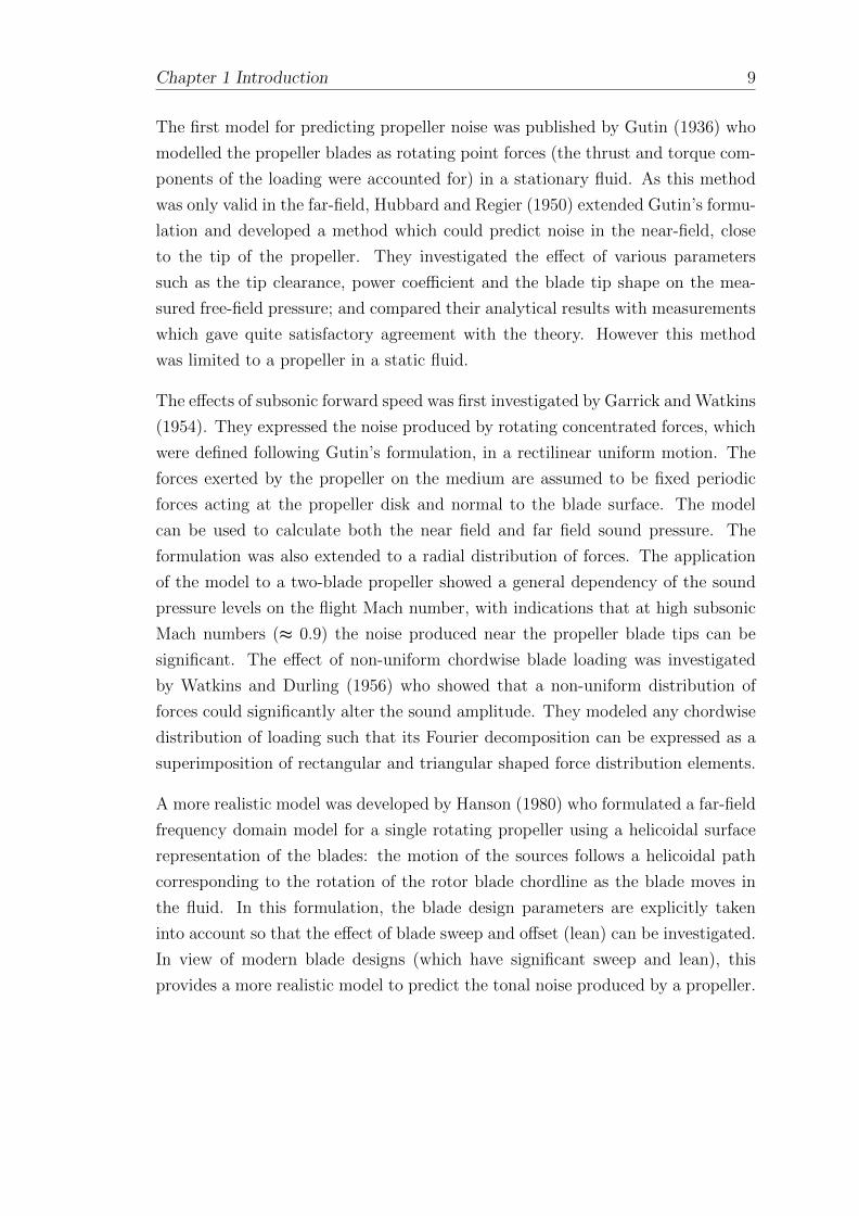
The first model for predicting propeller noise was published by Gutin (1936) who
modelled the propeller blades as rotating point forces (the thrust and torque com-
ponents of the loading were accounted for) in a stationary fluid. As this method
was only valid in the far-field, Hubbard and Regier (1950) extended Gutin’s formu-
lation and developed a method which could predict noise in the near-field, close
to the tip of the propeller. They investigated the effect of various parameters
such as the tip clearance, power coefficient and the blade tip shape on the mea-
sured free-field pressure; and compared their analytical results with measurements
which gave quite satisfactory agreement with the theory. However this method
was limited to a propeller in a static fluid.
The effects of subsonic forward speed was first investigated by Garrick and Watkins
(1954). They expressed the noise produced by rotating concentrated forces, which
were defined following Gutin’s formulation, in a rectilinear uniform motion. The
forces exerted by the propeller on the medium are assumed to be fixed periodic
forces acting at the propeller disk and normal to the blade surface. The model
can be used to calculate both the near field and far field sound pressure. The
formulation was also extended to a radial distribution of forces. The application
of the model to a two-blade propeller showed a general dependency of the sound
pressure levels on the flight Mach number, with indications that at high subsonic
Mach numbers (≈ 0.9) the noise produced near the propeller blade tips can be
significant. The effect of non-uniform chordwise blade loading was investigated
by Watkins and Durling (1956) who showed that a non-uniform distribution of
forces could significantly alter the sound amplitude. They modeled any chordwise
distribution of loading such that its Fourier decomposition can be expressed as a
superimposition of rectangular and triangular shaped force distribution elements.
A more realistic model was developed by Hanson (1980) who formulated a far-field
frequency domain model for a single rotating propeller using a helicoidal surface
representation of the blades: the motion of the sources follows a helicoidal path
corresponding to the rotation of the rotor blade chordline as the blade moves in
the fluid. In this formulation, the blade design parameters are explicitly taken
into account so that the effect of blade sweep and offset (lean) can be investigated.
In view of modern blade designs (which have significant sweep and lean), this
provides a more realistic model to predict the tonal noise produced by a propeller.

10 Chapter 1 Introduction
1.3 Contra-rotating open rotor or Advanced Open
Rotor (AOR)
When adding a second rotor, acoustic and aerodynamic interference occurs be-
tween the two blade rows. In addition to rotor-alone tones produced by each
single rotor, a number of interaction tones are produced by the interaction of the
distorted flow field of one rotor with the adjacent rotor. This causes the level of
noise emitted from an AOR to be much higher than an equivalent single-rotating
open rotor (Magliozzi and Hanson, 1991). Interaction tones occur at frequencies
corresponding to the sum or difference of integer multiples of the BPF of the two
rotors. The generation of interaction tones can be due to various sources, which
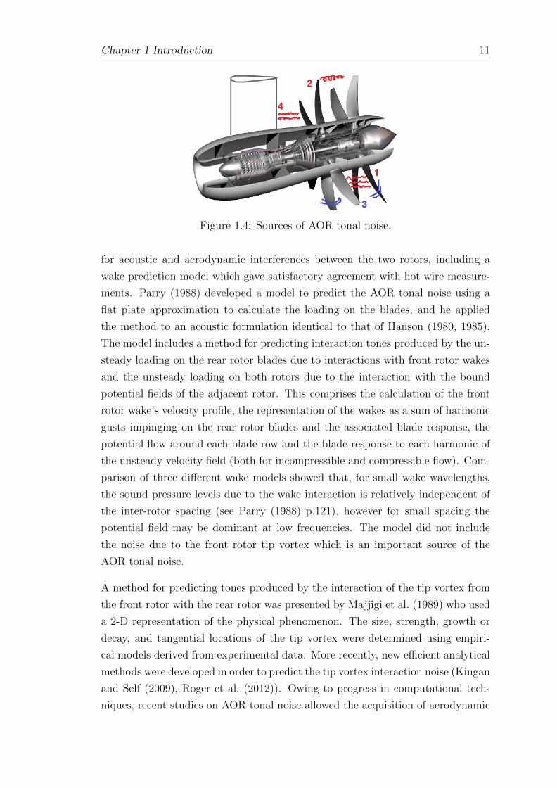
are illustrated in figure 1.4, such as:
1. The impingement of the upstream rotor’s viscous wakes onto the downstream
rotor.
2. The impingement of the upstream rotor’s tip vortices onto the downstream
rotor.
3. The interaction of the bound potential field of each rotor with the adjacent
rotor.
When installed on an aircraft, additional sources of tonal noise are produced. For
example, extra tonal noise is produced by the periodic loading on the rotor blades
due to rotor interaction with the flow distortion produced by nearby structures
such as a pylon (see the source labeled 4 in figure 1.4) or the change in the inflow
angle with respect to the engine shaft axis (i.e. the angle of attack). They can
significantly alter the noise produced by the AOR (Ricouard et al. (2010), Paquet
et al. (2014)).
The earliest study on AOR noise was published by Hubbard (1948), based on
Gutin’s theory. He highlighted the presence of the acoustic interference mech-
anism between the two blade rows: the phase difference between the propellers
blades could result in destructive or constructive interference patterns if tones were
produced by both rotors at the same frequencies. Hubbard did not include the
effect of an axial flow or the forward speed of the rotor in this model.
Hanson conducted numerous studies of open rotor tonal noise, and developed the
first comprehensive prediction model for AOR tonal noise. In addition to his he-
licoidal model, Hanson (1985b) developed a far-field analytical model to account
Chapter 1 Introduction 11
Figure 1.4: Sources of AOR tonal noise.
for acoustic and aerodynamic interferences between the two rotors, including a
wake prediction model which gave satisfactory agreement with hot wire measure-
ments. Parry (1988) developed a model to predict the AOR tonal noise using a
flat plate approximation to calculate the loading on the blades, and he applied
the method to an acoustic formulation identical to that of Hanson (1980, 1985).
The model includes a method for predicting interaction tones produced by the un-
steady loading on the rear rotor blades due to interactions with front rotor wakes
and the unsteady loading on both rotors due to the interaction with the bound
potential fields of the adjacent rotor. This comprises the calculation of the front
rotor wake’s velocity profile, the representation of the wakes as a sum of harmonic
gusts impinging on the rear rotor blades and the associated blade response, the
potential flow around each blade row and the blade response to each harmonic of
the unsteady velocity field (both for incompressible and compressible flow). Com-
parison of three different wake models showed that, for small wake wavelengths,
the sound pressure levels due to the wake interaction is relatively independent of
the inter-rotor spacing (see Parry (1988) p.121), however for small spacing the
potential field may be dominant at low frequencies. The model did not include
the noise due to the front rotor tip vortex which is an important source of the
AOR tonal noise.
A method for predicting tones produced by the interaction of the tip vortex from
the front rotor with the rear rotor was presented by Majjigi et al. (1989) who used
a 2-D representation of the physical phenomenon. The size, strength, growth or
decay, and tangential locations of the tip vortex were determined using empiri-
cal models derived from experimental data. More recently, new efficient analytical
methods were developed in order to predict the tip vortex interaction noise (Kingan
and Self (2009), Roger et al. (2012)). Owing to progress in computational tech-
niques, recent studies on AOR tonal noise allowed the acquisition of aerodynamic
12 Chapter 1 Introduction
data via various numerical schemes. Strip theory methods calculate the unsteady
field along several ‘strips’: the blade is split into several radial sections and the
incident flow field is assumed to be uniform on each of them. The aerodynamic
properties of the flow are then calculated for each blade section. CFD simulations
provide information on the flow behaviour around the blade geometry and may
deliver more accurate aerodynamic data. Carazo et al. (2011) used both meth-
ods to predict the wake interaction noise of an AOR. The blade segments were
modeled as trapezoids in unwrapped coordinates. The unsteady loading on each
section was calculated based on Amiet’s gust-airfoil response models (Amiet et al.,
1989) with inclusion of the spanwise variation of blade chord and sweep. Some
coefficients were determined using semi-empirical wake models. Comparison with
CFD simulations and wind tunnel measurements showed some disparities between
the methods. The analytical model seemed to over-predict the sound field whereas
better agreement with the measurements was found using the numerical computa-
tion. Some of the discrepancies between the analytical and the numerical results
were later on found to be influenced by the existence of a leading edge vortex
(Jaouani et al., 2016). A recent comparison between another strip theory code
and CFD by Kingan et al. (2014) showed that the aerodynamic inputs obtained
with CFD simulations gave better agreement with measurements than the data
obtained with the strip theory code. However obtaining high fidelity CFD data is
critical to accurately predict noise levels.
Due to the advances in research and efforts to reduce the tonal noise of the AOR,
the broadband noise has become an important contributor to the total sound
field (Parry et al., 2011). Although the present work focuses on tonal noise, it is
worth mentioning where the broadband noise originates from. Broadband noise
is thought to be produced by the unsteady stresses on the rotor blades due to
turbulence interacting with the rotor blades. Possible sources of broadband noise
which were identified in the literature (Blandeau, 2011) are:
1. The impingement of the turbulent component of the upstream rotor’s wakes
onto the leading edge of the downstream rotor’s blades.
2. The impingement of the upstream rotor’s turbulent tip vortices onto the
leading edge of the downstream rotor’s blades.
3. Turbulent ‘self-noise’, produced by the interaction of the turbulent boundary
layer on the surface of each rotor blade with the trailing edge.
4. Atmospheric turbulence ingestion.

Chapter 1 Introduction 13
5. The interaction of the turbulent component of a pylon’s wake with the front
rotor’s blades.
6. Hub boundary layer ingestion noise.
7. Secondary flow between the two rotors.
1.4 Installation effects
Most of the studies cited above do not take into account installation effects (angle
of attack, interactions with the flow field produced by structures such as the pylon,
fuselage, and the aircraft wings, tail sections), which cause significant changes in
the sound field produced by the propeller. This section illustrates the different
analyses that have been conducted to describe the sound field produced by an
installed AOR.
1.4.1 Angle of attack
The angle of attack (AOA) corresponds to the angle between the engine axis and
the flow (see figure 1.5). The noise produced by an AOR when operating at
angle of attack will be significantly different to that produced when the AOR is
at 0 AOA. The investigation of this effect started in the 1980s with experimental
studies of propeller blade passing frequency noise with angular inflow conducted by
Block (1986) and Woodward (1987). Block tested a lightly loaded propeller with
a relatively small number of blades and noticed an increase and a decrease in noise
levels respectively under and above a single rotating propeller at angle of attack,
in comparison with a propeller at zero angle of attack, and small changes in sound
pressure levels for a contra-rotating propeller at AOA. The results of Woodward
for a contra-rotating propeller with higher loading and number of blades (11 and
9) showed some important variations in the noise levels and directivity patterns of
an AOR at angle of attack compared to an AOR at zero angle of attack, notably
for the azimuthal variation of aerodynamic loading.
Stuff (1988) attempted to quantify the noise produced by a propeller at angle of
attack in a uniform flow using an analytical method. He showed that the angular
inflow significantly affects the directivity of the sound field with an increase in the
sound pressure level in the forward and downward directions. However, this was
applicable only for a point source.

14 Chapter 1 Introduction
Mani (1990) developed a model for predicting the sound field due to the unsteady
loading caused by the AOA. The model was compact in the chordwise direction.
The results were compared with the experiments of Block and Woodward and
showed that the sound pressure level produced by a propeller at angle of attack was
underestimated for the case of a highly loaded propeller (Woodward). Mani found
that, in addition to the unsteady loading, the AOA caused azimuthal variations
in the radiation efficiency of the propeller. Including this effect in his model, the
results were in a better agreement with Woodward’s measured data for an AOR.
However, the blade passing frequency of the rear rotor was still underestimated.
This may have been due to difficulties in accurately calculating the flow incident
on the rear rotor.
γ
Flow direction
Figure 1.5: Definition of the angle of attack.
Krejsa (1990) developed an analytical model to predict the noise produced by a
single rotation propeller at angle of attack, based on the derivation of Parry (1988)
for a propeller at zero angle of attack. The model was applicable to a larger range
of angles of attack in comparison to the study of Mani. The study confirmed that
in addition to the unsteady loading due to the inflow incidence, the inclusion of
the effects of angle of attack on the radiative efficiency of the loading and thickness
noise components improves agreement with the experiments. Unlike Parry’s model
(which was limited to the case of zero angle of attack), the location of the source
distribution was limited to the blade midchord i.e. the loading was modelled as
chordwise compact.
Other prediction methods for propeller and propfan noise at angle of attack have
been formulated, for example Envia (1991) who did not formulate a near or far-
field approximation but used a large blade count limit. The blade surface was
segmented into a large number of elements and the sound field of a propeller at

Chapter 1 Introduction 15
angle of attack was expressed in terms of Airy functions restricted to small AOA
(under 5 degrees). Blade design parameters were not explicitly specified in the
formulation. The work of Hanson and Parzych (1993) is the most complete and
comprehensive model available for modelling the far-field noise due to a propeller
at angle of attack. The model is based on Goldstein’s acoustic analogy (Goldstein,
1974). All sources of noise are considered including the radial contribution of the
loading (which is often ignored in prediction models). The monopole and dipole
sources are located on the blades surface and the quadrupole sources in the volume
around the blades. The previous simplifications for blade geometry have been
removed so the derivation provides an exact formulation of the propeller tonal
noise at angle of attack. Hanson (1995) extended this analysis to show that the
increase of radiation efficiency due to the crossflow was due to the increase of the
source Mach number relative to the observer caused by the propeller tilt. The
work presented in this thesis is based on the former model (Hanson and Parzych
(1993)) with simplification of the blade geometry.
The effects of the angle of attack on the noise produced by an AOR was investi-
gated by Brandvik et al. (2012). The interest was to describe the altered velocity
profile and loading distribution in between the two rotors. They conducted CFD
simulations for an AOR at take-off and observed significant changes in the flow
field due to the angle of attack, notably for angles of attack greater than 3 (the
AOA varied from 0 to 12). They investigated the effect of the rotor AOA on
the front rotor viscous wake and tip vortex interaction sources. It was clearly
shown that the angle of attack induces circumferential variations in the front ro-
tor’s wakes and in the strength and size of the tip vortex. The acquisition of
high fidelity aerodynamic data at angle of attack would thus be of interest for the
present study in order to predict the tip vortex and wake profiles between the two
rotors.
1.4.2 Fuselage scattering
When the AOR is mounted on the aircraft, the interaction of the incident sound
field with the fuselage can have a significant effect on the radiated noise. This effect
must be taken into consideration when predicting the total sound field produced
by an installed AOR.
To the author’s knowledge, the first consideration of the effect of the aircraft
fuselage was made by Hubbard and Regier (1950) who investigated the fuselage

16 Chapter 1 Introduction
response to the oscillating pressures produced by an adjacent propeller. They
conducted experiments modelling the fuselage as a flat vertical wall and a circular
wall. The tests showed a considerable increase in the sound pressure levels pro-
duced by the propeller due to the presence of the walls, with a larger increase for
the vertical wall which is not a realistic representation of the fuselage geometry.
The analysis provides calculations of the vibration amplitude of the panel as a
function of its mass, natural frequency and structural damping.
The presence of the fuselage can engender shielding effect. The latter was identified
during flight tests of a propfan mounted on a Jetstar business aircraft, see Hanson
(1984) who made the first attempt to model the shielding effect of the fuselage
boundary layer. His study treated plane incident waves on a flat plate, which is a
crude approximation for a fuselage but was suitable for a preliminary study. The
results showed that the boundary layer provided shielding upstream of the rotor
and that the shielding effect increased with the boundary layer thickness.
Hanson and Magliozzi (1985) developed a more advanced frequency-domain method
to assess the effect of the refraction and scattering of propeller tones by the air-
craft fuselage and boundary layer. The fuselage was modelled as an infinite rigid
cylinder to simplify the analysis. The boundary layer profile was assumed to be
constant around the circumference of the cylinder and also axially. The incident
sound field was calculated using Hanson’s near-field theory for propellers (Hanson
(1985a)), the acoustic field inside the fuselage boundary layer was calculated by
solving a form of the Pridmore-Brown equation, and the solutions inside and out-
side the boundary layer were matched. The method can be utilised to calculate
the noise levels at the fuselage surface, which can then be used to evaluate cabin
noise. Fuller (1989) derived a simple formulation considering the scattering effects
of an infinite rigid cylinder (with no boundary layer) for stationary monopole and
dipole acoustic sources. Lu (1990) extended Hanson and Magliozzi’s model to de-
termine the noise emission both on the fuselage surface and in the far field using
an asymptotic solution. More recently McAlpine and Kingan (2012) studied the
effect of fuselage scattering on the noise emitted by a rotating point source and an
open rotor (modeled as distributed sources). They applied Hanson and Magliozzi’s
formulation neglecting the fuselage boundary layer. They showed evidence that
the far-field directivity of an open rotor is affected by the source rotational di-
rection, location and distance from the fuselage. More recently, Brouwer (2016)
presented a method to estimate the scattering of open rotor tones by a rigid cylin-
drical cylinder including its boundary layer. He developed a simplified model to
reproduce the directivity and propagation properties of an AOR. He showed that
Chapter 1 Introduction 17
the presence of the boundary layer causes reductions of acoustic pressure levels on
the fuselage upstream of the AOR as well as variations of SPL with circumferential
angle in both the near-field and the far-field. Although the source modelling is
not truly representative of the noise radiated from an installed AOR, the method
provides quick estimates of the scattered sound field.
1.4.3 Wing and pylon
The presence of an upstream pylon or a downstream wing can significantly influ-
ence the noise produced by an AOR. The pylon generates a potential field and
viscous wakes upstream of the rotors, which produces additional sources of noise.
The presence of a wing would produce supplementary flow distortions and scat-
tering.
Only a few studies on pylon and wing installation effects were identified by the
author. Tanna et al. (1981) conducted experiments on an installed single rotation
propeller and highlighted an increase in tonal noise as a result of the inflow dis-
tortions due to the upwash induced by a downstream wing. Amiet (1986, 1991)
studied the diffraction of sound radiated from a point source by a half plane in a
uniform flow and derived analytical solutions for both swept and unswept wings.
The latter was used by Kingan and Self (2012) to describe the scattering of the
sound from a rotating point source by a rigid half plane in a stationary medium,
and extended to the case of distributed sources in a moving medium. They ap-
plied this method to assess the scattered sound field of an open rotor. For an open
rotor mounted above the wing, the sound pressure levels are significantly reduced
by the presence of the half-plane, which is a promising solution for current and
future noise reduction schemes.
Shivashankara et al. (1990) conducted tests of a scale model of the UDF engine
and investigated the influence of the presence of an upstream pylon on the noise
field of this AOR. They noticed an increase of up to 10-12 dB of the blade pass-
ing frequency tones but negligible variations on the interaction tones. Recent
experiments by Ricouard et al. (2010) lead to similar observations: the pylon sig-
nificantly affects the rotor-alone tones (especially the front rotor BPF) but has a
negligible effect on rotor-rotor interaction tones. Furthermore, results showed that
the polar and azimuthal directitivies of the AOR sound field were greatly affected
by the pylon, and that the velocity profile of the pylon wake, which appeared to

18 Chapter 1 Introduction
significantly influence the sound field, could be reduced by the application of py-
lon trailing edge blowing. This benefit was highlighted in by Paquet et al. (2014)
whose experimental data analysis showed that the pylon blowing was more effec-
tive at low thrust than at high thrust. More recently Sinnige et al. (2015) analysed
the effects of pylon blowing on the noise emissions and the propulsive performance
of a propeller in a pusher configuration using Particle Image Velocimetry (PIV)
measurements. Again, the application of pylon blowing proved to be beneficial,
using appropriate blowing coefficients. The influence of the pylon design is thus
an interesting subject of research to reduce the noise produced by a AOR. In their
study of the scattered field of an open rotor by a fuselage McAlpine and Kingan
(2012) included a representation of a pylon wake in terms of an impulsive loading
component. They pointed out that the noise could be reduced at certain observer
locations depending on the position of the pylon. They also found that the noise
radiated by the open rotor was affected by the pylon length, as it is directly re-
lated to the distance between the source and the fuselage. More recently, Jaouani
et al. (2015) developed a semi-analytical model to predict the effect of the pylon
wake on the front rotor-alone tones radiated by an AOR in a pusher configuration.
The pylon wake in the vicinity of the front rotor leading edge and the unsteady-
loading on the front rotor blades were determined numerically, and the radiated
sound field was calculated analytically. The model included the computation of
the steady-loading and thickness noise, which appeared to interfere significantly
with the unsteady-loading noise caused by the pylon wake.

Chapter 1 Introduction 19
1.5 Aims, objectives and original contributions
A thorough assessment of the noise produced by an advanced open rotor (AOR)
would require precise theoretical and computational models supplemented with
truly representative wind-tunnel tests. As the implementation of such tests is a
long and expensive process, the development of efficient analytical and numerical
prediction methods enables fast analysis of the AOR’s noise, and thus is a useful
asset for aircraft manufacturers. An existing prediction model for tonal noise is
currently used by Rolls-Royce plc. The aim of the present project is to develop
a new prediction method which can be used to calculate the far-field tonal noise
produced by an advanced open rotor, as it remains a major contributor to the
total noise, and which can be implemented into the existing tools.
The first objective is to predict the unsteady loading noise produced by an isolated
advanced open rotor at angle of attack relative to the aircraft flight path.
The second objective is to use Computational Fluid Dynamics (CFD) data to
validate the unsteady loading calculation methods and to predict interaction tones
produced by an isolated AOR. Of particular interest is to quantify the differences
between current and new prediction methods using various aerodynamic input
data.
The third objective is to develop methods to analyse experimental data and to
validate the analytical models against test measurements.
Accordingly, in the thesis the material is ordered as follows. The data analysis is
presented in Chapter 2.
Next, the detailed derivation of the loading noise produced by a propeller at angle
of attack is presented in Chapter 3.
The derivation of the interaction tone noise radiation expressions is detailed in
Chapter 4.
In Chapter 5 a hybrid analytical/numerical method for predicting wake interac-
tion noise is described. The method utilizes predictions from a three-dimensional
CFD simulation of an advanced open rotor rig to acquire the wake characteristics
at a particular location in the inter-rotor region. An analytical model is used to
propagate the wake profiles to the leading edge of the downstream rotor blades.
The blade response is then calculated used in an analytical method to predict the
far-field noise.
In Chapter 6 a model is derived to predict the noise produced by the interac-
tion between the potential field of one rotor and the adjacent rotor, considering
20 Chapter 1 Introduction
both the thickness and the loading problems. The model is compared with exist-
ing methods and the relative contribution of wake and potential field interaction
tones is assessed.
Finally, it is noted that the experimental results are compared with predictions in
both Chapters 5 and 6. Concluding remarks are then given in Chapter 7.
The original contributions in the thesis are highlighted below:
1. Development of a method to post-process wind tunnel experimental data.
Creation of algorithms specific to the format of the data collected during
Rolls-Royce’s latest test campaigns. Extensive analysis of the data, of which
one part is presented in this thesis and the second part was provided to
Rolls-Royce via a proprietary deliverable.
2. Development of a simple and fast prediction method for predicting the far-
field tonal noise produced by a propeller at angle of attack.
3. Development of a numerical routine to post-process CFD data specifically to
the delivered format. This includes the extraction of the flow disturbances
associated with each rotor in moving and stationary frames, around the
blades and in the inter-rotor region.
4. Development of a hybrid analytical/computational method for predicting
wake interaction noise. The novel contribution of this method is the ana-
lytic propagation of CFD wakes in order to calculate the downstream blade
response and the radiated noise. The assessment of the analytic development
of the wake characteristics in the inter-rotor region relative to that given by
the CFD.
5. Extension of existing methods for predicting the noise produced by potential
field interactions in an AOR. The method models the potential field of each
rotor blade using a distribution of sources along the rotor blade chordline.
Chapter 2
Model scale open rotor data
analysis
A number of experimental test campaigns using model scale advanced open ro-
tors have recently been undertaken in the German-Dutch Wind Tunnels (DNW)
Large Low-speed Facility (LLF), the Netherlands. The first of the recent experi-
mental campaigns was undertaken in 2008 as a part of the EU project DREAM
(“valiDation of Radical Engine Architecture SysteMs”), and used Rolls-Royce’s
one-sixth scale advanced open rotor rig (known as Rig 145 Build 1). A second
experimental campaign using the same rig but with aeroacoustically optimised
blades (known as Rig 145 Build 2) was undertaken in 2010. More recently, tests
were run as a part of the Clean Sky Joint Technology Initiative (JTI) EU pro-
gramme in 2012-2013 using a one-seventh scale advanced open rotor rig designed
by Airbus (known as the Z08 rig) at the DNW wind tunnel. The tests of interest
in this Chapter were conducted on Airbus’ Z08 rig mounted with blades designed
by Rolls-Royce. Extensive analysis was performed for different pitch and thrust
settings. The author’s contribution to this study is described in this chapter. The
principal tasks involved the post-processing and the analysis of experimental data
from the Rig145 Build 2 and Z08 experimental test programmes.
2.1 Description of the wind tunnel facility
The DNW LLF wind tunnel is located in Marknesse, the Netherlands. It is a closed
circuit, continuous low-speed wind tunnel in which flight operating conditions such
as take-off, approach and cutback can be tested. The forward flight simulation
21

22 Chapter 2 Model scale open rotor data analysis
is produced by an open jet of variable cross-section. It is capable of providing
continuous jet velocities up to 152m/s for the smallest jet section (6m× 6m).
The instrumentation used for both the Rig 145 Build 2 and Z08 experiments com-
prises far-field out-of-flow microphone arrays located in the roof, walls, floor and
the door of the facility, as well as inflow microphones mounted on a traversing
system specific to each test campaign. A description of the set-up for the Rig 145
Build 2 tests is shown in figure 2.1.
Figure 2.1: Schematic showing the experimental test set-up during testingof Rig 145 Build 2 in the DNW wind tunnel. Published in Parry et al.(2011).
2.1.1 Rig 145 Build 2 test campaign
The objective of this campaign was to measure and analyse the noise produced by a
contra-rotating open rotor and to assess the quality of the acoustic measurement
method. The experiments were conducted using Rolls-Royce’s one-sixth scale
advanced open rotor with respectively 12 and 9 front and rear rotor blades. The
series of tests was run with an open jet nozzle measuring 8m×6m with a Mach
number of approximately 0.2. A set of 1/2” and 1/4” inflow microphones was
mounted on a C-shaped traversing frame located at a fixed sideline distance from
the open rotor rig. The data collected from the inflow microphones was recorded
as the traverser translated upstream and downstream of the open rotor rig. This
enabled coverage at a wide range of polar and azimuthal locations. Similarly, a

Chapter 2 Model scale open rotor data analysis 23
series of out-of-flow microphones were mounted on the traverser. A photograph
of the experimental setup is shown in figure 2.2, and the traversing system is
described in figure 2.3.
Figure 2.2: Rig145 Build 2 installed in the DNW wind tunnel. Publishedin Parry et al. (2011).
The experiments were conducted for the following configurations:
• Isolated rig (uninstalled): The effect of varying parameters such as the flow
Mach number, the propeller rotational speeds, the blade pitch angles was
investigated.
• Isolated rig with variation of the angle of attack: The same parameters as
the uninstalled case were investigated.
Note that the previous Rig145 Build 1 experiments also tested an isolated rig with
a pylon. The same parameters as the uninstalled case could be modified as well as
the location of the pylon. A set up including an Airbus designed blowing system
was also added. Its effect was investigated and described in details by Ricouard
et al. (2010), see section 2.3.3.
24 Chapter 2 Model scale open rotor data analysis
Figure 2.3: Traversing system used for Rig145 tests in the DNW windtunnel. Published in Parry et al. (2011).
2.1.2 Z08 rig test campaign
The aim of the Z08 experimental campaign was to investigate the effects of in-
stallation on the sound emitted from an advanced open rotor, and to measure the
noise produced by a number of different AORs operating at different conditions.
This campaign was, with the support of the EU funding Clean Sky, a collaboration
between the manufacturers Airbus, Rolls-Royce and Snecma. The engine used for
the experiments was Airbus Z08 air turbine driven rig, for which different sets of
blades were provided by Airbus, Rolls-Royce and Snecma. The present Chapter
focuses on the Rolls-Royce/Airbus phase. The rotor geometry was taken from
open rotor one-seventh scale 12x9 blades designed by Rolls-Royce to fit onto the
Z08 rig. The data from the Rolls-Royce/Airbus phase is jointly owned by Airbus
and Rolls-Royce, who have given the author the permission to use them in the
present thesis. Note that the Airbus phase (utilizing Airbus’ generic 11x9 blades
called AI-PX7) is described further in details by Paquet et al. (2014).
The inflow microphones used to measure the pressure levels around the engine were
mounted on a wing-shaped horizontal traverser (see an example of a test configu-
ration in figure 2.6). This instrumentation comprised a set of inflow wire-mesh and
flush-mounted microphones. The wire-mesh microphones are mounted in a cavity
with the upper surface closed by a porous mesh (see figure 2.4). The presence
of the mesh suppresses the noise due to the turbulent flow at the panel surface.
The mesh is relatively impermeable to the flow passing over the traverser but is
effectively acoustically transparent. Pressure perturbations due to the turbulent

Chapter 2 Model scale open rotor data analysis 25
hydrodynamic flow decay evanescently within the cavity. Thus the microphone
at the bottom of the cavity measures little flow noise. However, because the mi-
crophone is located within the cavity, the signal measured by these microphones
will be dependent on the angle of incidence of the acoustic waves. This effect is
not taken into account in the analysis presented here and may account for some
of the differences observed between the measurements of the wire-mesh and the
flush mounted microphones in Section 2.4.2.
microphonemesh
turbulentflow
Figure 2.4: Sketch of a wire-mesh microphone mounted on an airfoil.
The flush-mounted microphones have their diaphragm aligned with the upper
surface of the traverser airfoil and so these microphones measure the pressure per-
turbation due to the turbulent boundary layer in addition to the incident acoustic
pressure (see figure 2.5). They can capture the tonal noise in all directions, pro-
vided that the level of the tones is greater than the aerodynamic noise.
microphone
turbulentflow
Figure 2.5: Sketch of a flush-mounted microphone on an airfoil.
The test data was collected for the following configurations:
• Isolated rig (uninstalled): Test parameters such as the flow Mach number,
the propeller rotational speeds, the blade pitch angles, the inter-rotor spac-
ing, and number of blades could be modified. Additional sets of blades were
provided by Rolls-Royce and Snecma in order to assess the engine’s acoustic
sensitivity to the blade design.
• Isolated rig with variation of the angle of attack: The same parameters as
the uninstalled case could be modified.
• Rig installed with a downstream wing (puller configuration): The wing
sweep, angle of attack, distance from the propellers and the parameters
previously cited could be modified.
26 Chapter 2 Model scale open rotor data analysis
• Rig attached to an upstream pylon (pusher configuration): The position of
the pylon and the same parameters as the uninstalled case could be modified.
• Full aircraft tests. In addition to the parameters previously cited, the pres-
ence of landing gear, the slat and flap settings and parameters for pylon
blowing could be modified.
Investigation of the effect of the last two configurations was recently published by
Paquet et al. (2014) who confirmed that the pylon blowing system can be used to
significantly reduce the noise caused by the interaction of the pylon wakes with
the front rotor blades.
Figure 2.6: Z08 rig installed with a pylon in the DNW LLF wind tunnel.Note that in this picture the rig is mounted with Airbus’ blades. Publishedin Paquet et al. (2014).
Chapter 2 Model scale open rotor data analysis 27
2.2 Acoustic data processing
The data analysis was conducted using a post-processing routine developed by the
author. This routine is suitable for analysing either Rig 145 or Z08 data, as the
data format is common for both test campaigns. Note that a preliminary correction
for propagation distance was made by Rolls-Royce so that each microphone is
calibrated to measure the noise of the contra-rotating propeller at a reference
radiation distance (emission radius) of 16.6 meters. The correction was performed
using the inverse-square law based on the principle that the acoustic intensity is
inversely proportional to the square of the radiation distance. To be applicable,
the method assumes a spherical spreading of the sound waves and no reflections or
reverberation effects in the wind tunnel. Note that as far-field results for an AOR
are generally expressed in terms of emission coordinates, all the measurements
are presented in the emission coordinate system. A conversion from reception to
emission coordinates is described in the following section.
2.2.1 Emission and reception coordinate systems
When the aircraft is flying, the noise emission time differs from the reception time
at the observer position. In fact, when the observer receives the noise at time t,
it corresponds to a position of the aircraft at time t −∆t where ∆t = re/c0 , re is
the distance at emission time between the observer and the aircraft, and c0 the
sound propagation speed. In propeller noise studies, we often use the emission
(or retarded) coordinate system. Figures 2.7(a) and 2.7(b) describe the emission
and reception coordinate systems for the flyover case and in a wind tunnel. In a
wind tunnel, as the propeller is fixed in a moving flow, the emission position will
correspond to a virtual source position.
Let (xr, r, θ) and (xe, re, θ′) be the axial, radial and polar coordinates at reception
and emission time respectively. The origin of both coordinate systems is defined
on the engine axis and half way between the two rotors. The coordinate systems
are represented in figure 3.3. Let M be the flow Mach number in the positive axial
direction, and R the sideline radius. As the sound wave propagates during the
time ∆t, the acoustic wave front is convected by the flow by a distance ∆r = Mre.
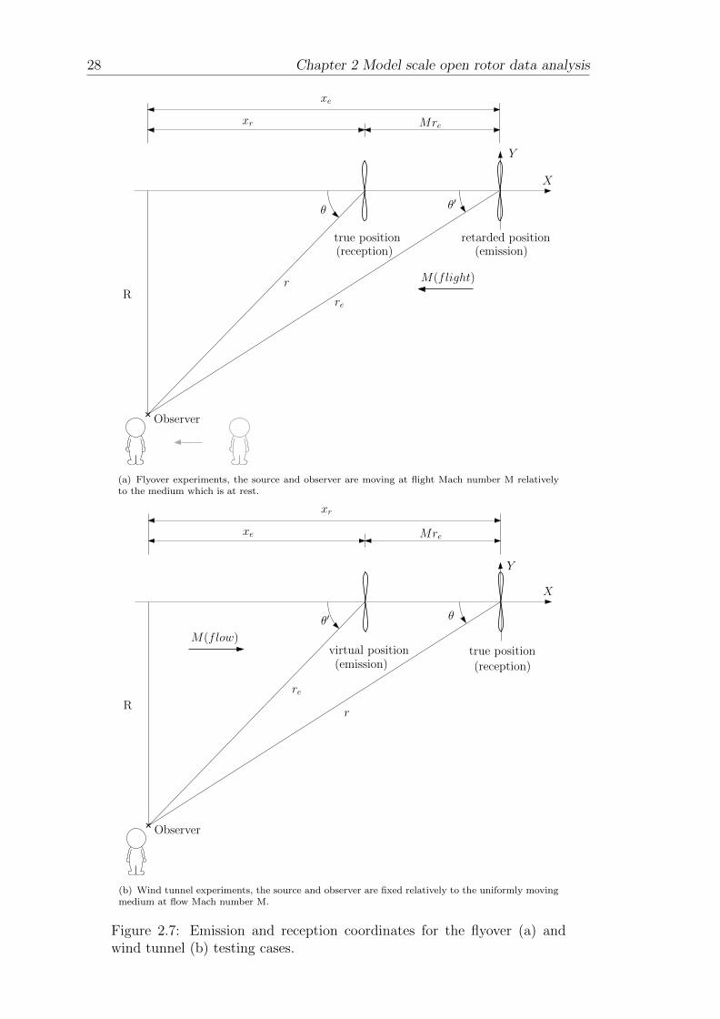
28 Chapter 2 Model scale open rotor data analysis
xe
Rre
Mrexr
θ θ′
Y
X
retarded positiontrue position
Observer
M(flight)
(emission)(reception)
r
(a) Flyover experiments, the source and observer are moving at flight Mach number M relativelyto the medium which is at rest.
xr
R
re
Mrexe
θ′ θ
Y
X
virtual position true position
Observer
M(flow)
r
(reception)(emission)
(b) Wind tunnel experiments, the source and observer are fixed relatively to the uniformly movingmedium at flow Mach number M.
Figure 2.7: Emission and reception coordinates for the flyover (a) andwind tunnel (b) testing cases.

Chapter 2 Model scale open rotor data analysis 29
The reception coordinates xr and r can be defined in terms of emission coordinates
as
xr = −re cos θ′ + ∆r = re(cos θ −M), (2.1)
R = re sin θ′. (2.2)
To convert from reception to emission coordinates we consider the relationships
xe = −xr + ∆r = −R cos θ′, (2.3)
re2 = (−xr + ∆r)
2 +R2 = (Mre − xr)2 +R2, (2.4)
θ′ = cos−1
(Mre − xr
re
). (2.5)
Equation 2.4 leads to the following quadratic equation
(M2 − 1)re2 − 2xrMre + (xr
2 +R2) = 0. (2.6)
The solutions of equation 2.6 are given by
re =xrM ±
√xr2M2 − (M2 − 1)(xr2 +R2)
M2 − 1. (2.7)
Only the solution which gives positive values of re is used in the present case since
a negative emission radius would be nonphysical.
2.2.2 Post-processing methods
The post-processing method developed by the author consists in five steps. These
are described in the following and illustrated in figures 2.8 to 2.12.
Correction for background noise
The data collected during the tests comprise a set of ’raw’ measured noise
data of the operating AOR and a set of background noise levels. For each
test, the corresponding background noise levels were measured running a
‘blank’ test at identical Mach number during which the engine was driven
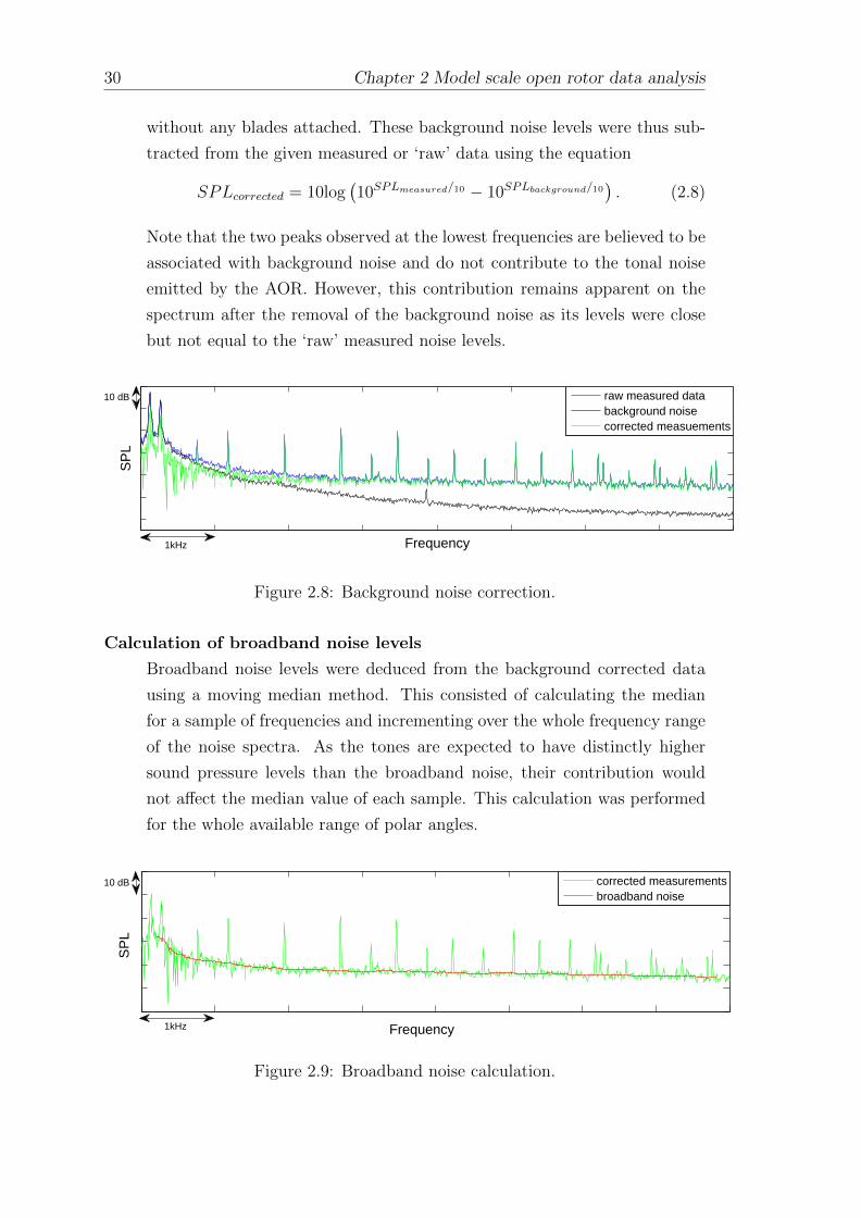
30 Chapter 2 Model scale open rotor data analysis
without any blades attached. These background noise levels were thus sub-
tracted from the given measured or ‘raw’ data using the equation
SPLcorrected = 10log(10SPLmeasured/10 − 10SPLbackground/10
). (2.8)
Note that the two peaks observed at the lowest frequencies are believed to be
associated with background noise and do not contribute to the tonal noise
emitted by the AOR. However, this contribution remains apparent on the
spectrum after the removal of the background noise as its levels were close
but not equal to the ‘raw’ measured noise levels.
Frequency
SP
L
raw measured databackground noisecorrected measuements
1kHz
10 dB
Figure 2.8: Background noise correction.
Calculation of broadband noise levels
Broadband noise levels were deduced from the background corrected data
using a moving median method. This consisted of calculating the median
for a sample of frequencies and incrementing over the whole frequency range
of the noise spectra. As the tones are expected to have distinctly higher
sound pressure levels than the broadband noise, their contribution would
not affect the median value of each sample. This calculation was performed
for the whole available range of polar angles.
SP
L
corrected measurementsbroadband noise
Frequency
10 dB
1kHz
Figure 2.9: Broadband noise calculation.

Chapter 2 Model scale open rotor data analysis 31
Identification of the tones
In order to distinguish the tones from the broadband noise in the measured
spectra using an automated procedure, a filter was applied to select only
the background corrected data whose levels were 3 dB above the broadband
noise levels.
Frequency
SP
L
corrected measurementsbroadband noisetones
1kHz
10 dB
Figure 2.10: Tones identification.
Correction for broadband noise
The contribution of the broadband noise was removed from the filtered data
by subtracting the broadband noise levels from the tones data in a similar
manner as equation 2.8 (yielding to slightly different sound pressure levels
close to the broadband noise levels, as shown in figure 2.11).
Frequency
SP
L
corrected measurementsbroadband noisetones
1kHz
10 dB
Figure 2.11: Broadband noise correction.

32 Chapter 2 Model scale open rotor data analysis
Unbroadening of the tones
The data obtained from the filtering tended to be spread amongst the fre-
quencies neighbouring the relevant tone frequency. The tones’ levels were
calculated by summing the energies contained within the adjacent frequency
bands, thereby deducing the level at each discrete frequency tone.
Frequency
SP
L
corrected measurementsbroadband noisetones
1kHz
10 dB
Figure 2.12: Tones unbroadening.
The post-processing method determines the polar directivities of any tone, pro-
vided that their level is high enough relatively to the background noise level.
In addition, the method provides broadband noise directivity patterns at any fre-
quency, and noise spectra at any polar angle within the measured range. The noise
spectra were initially measured at successive frequency bandwidths of 6.25Hz. A
conversion to one-third octave band spectra was implemented in order to have a
quick overview of the tones and broadband noise contribution to the total noise.

Chapter 2 Model scale open rotor data analysis 33
2.3 Measurement issues
2.3.1 Haystacking
The present analysis is restricted to inflow data as the measurement of tones
by out-of-flow microphones could be altered by reflections from nearby struc-
tures, background noise, atmospheric absorption, refraction and most importantly
haystacking. Haystacking, or the spectral broadening of tones, occurs when the
sound waves propagate though the jet shear layer. The tones amplitudes are re-
duced and, centered on each tone, a broadband bump or ”haystack” is measured
in the narrow band spectrum. The haystacking is considered ’weak’ when the
proportion of scattered energy is small compared to the energy remaining in the
tone and ’strong’ when the tone becomes undetectable and is replaced by a broad-
band hump. In wind tunnel experiments, the measurements from out-of-flow
flow direction
turbulent
AOR rig
shear layer
Figure 2.13: Scattering effects in a wind tunnel.
microphones can be significantly affected by haystacking. Figure 2.14 shows a
comparison of ’raw’ measurements captured from an inflow and an out-of-flow mi-
crophone during the Rig 145 tests. The spectral broadening of the tones captured
by the out-of-flow microphones is clearly visible and tends to become greater at
high frequencies. Two effects can be observed:

34 Chapter 2 Model scale open rotor data analysis
1. A loss in the tones protrusion.
2. An increase in the broadband noise levels.
These effects are a specific issue for out-of-flow measurements, which can lead to
errors in the evaluation of the tones and broadband noise. As the correction of
such data is not of concern here, the analysis is focused on data measured by inflow
microphones.
Frequency
SP
L
InflowOut−of−flow
2kHz
10 dB
Figure 2.14: Narrow band SPL spectrum at 90 of an inflow and an out-of-flow microphone at the same take-off case - Rig 145 tests.
The prediction of tones haystacking has been of concern in recent studies. McAlpine
et al. (2013) developed an analytical model to predict and quantify the spectral
broadening of the tones radiating from the exhaust nozzle of turbofan engines.
This method was developed using a weak-scattering formulation (Powles et al.,
2010) and provided encouraging results for which the features of the tones broad-
ening were well reproduced. This method can be applied to predict the tones
detected by the out-of-flow microphones provided that the scattering is ’weak’.
In figure 2.14 weak scattering is observed at low to medium frequencies. How-
ever once we move to the high frequency range, the tones energy collapse into the
haystacks (strong scattering) and numerous tones cannot be detected. Numerical
approaches were developed by Ewert et al. (2008) and more recently Clair and
Gabard (2015) who, based on the work of Ewert, analysed the scattering of a
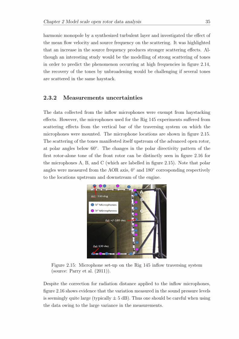
Chapter 2 Model scale open rotor data analysis 35
harmonic monopole by a synthesized turbulent layer and investigated the effect of
the mean flow velocity and source frequency on the scattering. It was highlighted
that an increase in the source frequency produces stronger scattering effects. Al-
though an interesting study would be the modelling of strong scattering of tones
in order to predict the phenomenon occurring at high frequencies in figure 2.14,
the recovery of the tones by unbroadening would be challenging if several tones
are scattered in the same haystack.
2.3.2 Measurements uncertainties
The data collected from the inflow microphones were exempt from haystacking
effects. However, the microphones used for the Rig 145 experiments suffered from
scattering effects from the vertical bar of the traversing system on which the
microphones were mounted. The microphone locations are shown in figure 2.15.
The scattering of the tones manifested itself upstream of the advanced open rotor,
at polar angles below 60. The changes in the polar directivity pattern of the
first rotor-alone tone of the front rotor can be distinctly seen in figure 2.16 for
the microphones A, B, and C (which are labelled in figure 2.15). Note that polar
angles were measured from the AOR axis, 0 and 180 corresponding respectively
to the locations upstream and downstream of the engine.
Figure 2.15: Microphone set-up on the Rig 145 inflow traversing system(source: Parry et al. (2011)).
Despite the correction for radiation distance applied to the inflow microphones,
figure 2.16 shows evidence that the variation measured in the sound pressure levels
is seemingly quite large (typically ± 5 dB). Thus one should be careful when using
the data owing to the large variance in the measurements.
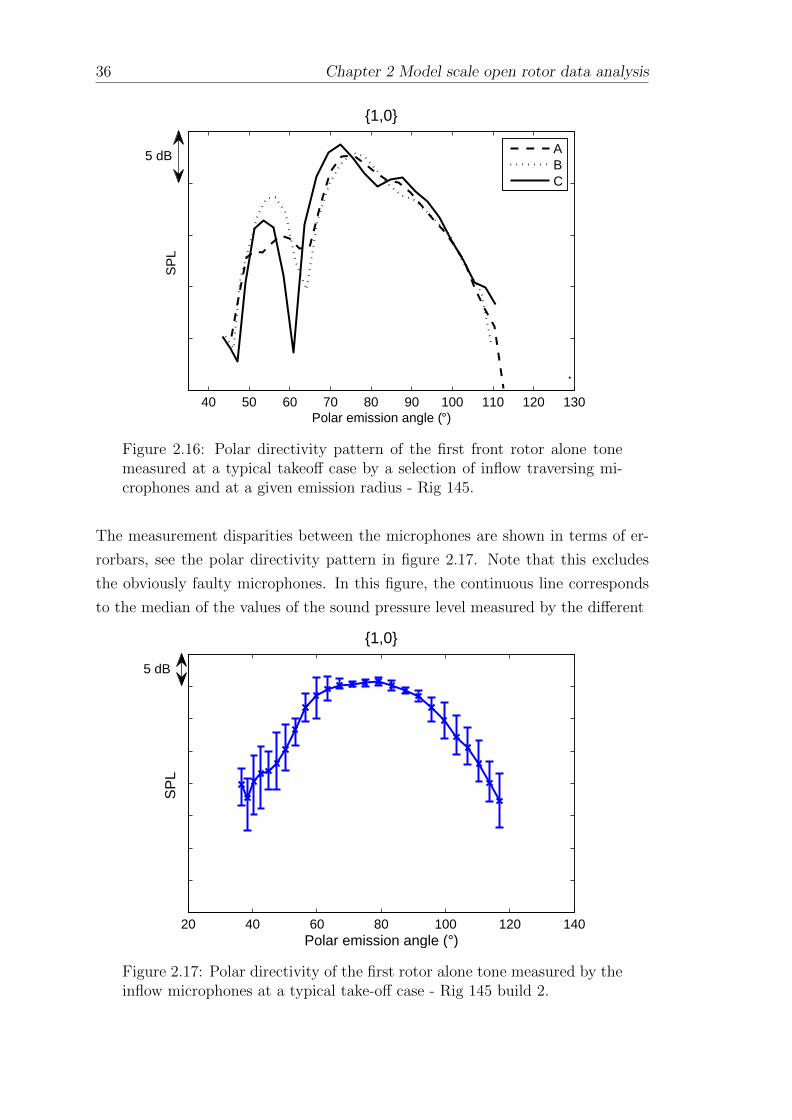
36 Chapter 2 Model scale open rotor data analysis
40 50 60 70 80 90 100 110 120 130Polar emission angle (°)
SP
L
1,0
ABC
5 dB
Figure 2.16: Polar directivity pattern of the first front rotor alone tonemeasured at a typical takeoff case by a selection of inflow traversing mi-crophones and at a given emission radius - Rig 145.
The measurement disparities between the microphones are shown in terms of er-
rorbars, see the polar directivity pattern in figure 2.17. Note that this excludes
the obviously faulty microphones. In this figure, the continuous line corresponds
to the median of the values of the sound pressure level measured by the different
20 40 60 80 100 120 140Polar emission angle (°)
SP
L
1,0
5 dB
Figure 2.17: Polar directivity of the first rotor alone tone measured by theinflow microphones at a typical take-off case - Rig 145 build 2.
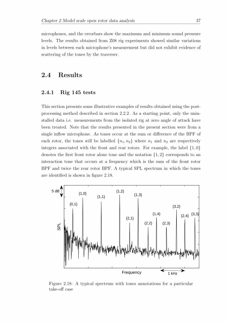
Chapter 2 Model scale open rotor data analysis 37
microphones, and the errorbars show the maximum and minimum sound pressure
levels. The results obtained from Z08 rig experiments showed similar variations
in levels between each microphone’s measurement but did not exhibit evidence of
scattering of the tones by the traverser.
2.4 Results
2.4.1 Rig 145 tests
This section presents some illustrative examples of results obtained using the post-
processing method described in section 2.2.2. As a starting point, only the unin-
stalled data i.e. measurements from the isolated rig at zero angle of attack have
been treated. Note that the results presented in the present section were from a
single inflow microphone. As tones occur at the sum or difference of the BPF of
each rotor, the tones will be labelled n1, n2 where n1 and n2 are respectively
integers associated with the front and rear rotors. For example, the label 1, 0denotes the first front rotor alone tone and the notation 1, 2 corresponds to an
interaction tone that occurs at a frequency which is the sum of the front rotor
BPF and twice the rear rotor BPF. A typical SPL spectrum in which the tones
are identified is shown in figure 2.18.
Frequency
SP
L
2,1
1,31,2
1,11,0
0,1
2,2
1,4
2,3
3,2
2,4
5 dB
1 kHz
3,3
Figure 2.18: A typical spectrum with tones annotations for a particulartake-off case

38 Chapter 2 Model scale open rotor data analysis
Influence of rotor speed
Test data was collected for several “pitch-lines”. One pitch-line corresponds to one
specified blade setting. Each pitch-line is denoted by a label P1×P2 corresponding
to the increase in rotational speed (RPM) of the rotor at take-off relative to its
design cruise rotational speed. We denote F the speed-up factor. A series of take-
off, approach and cutback cases were simulated for each pitch line with different
rotational speeds in order to reach the required full-scale thrust and a specific
torque-split between the two rotors. Although the main objective of the data
analysis is to be able to validate the current and future prediction methods against
experimental data, it is interesting to assess the influence of varying the rotors’
rotational speed on the noise. Indeed, as the same thrust can be reached using
different rotor blade pitch settings and rotational speeds, these parameters may
be of interest to optimise flight operating conditions.
Figures 2.19 to 2.21 show the polar directivity of the first rotor-alone tone produced
by the front rotor, 1, 0, and also some interaction tones at take-off, approach
and cutback at a constant emission radius. As expected, the sound pressure level
is higher as the thrust is larger, the take-off case being the loudest. Note that the
tones at approach condition could not be captured properly as the measurements
20 40 60 80 100 120 140Polar emission angle (°)
SP
L
1,0
take−offcutbackapproach
5 dB
Figure 2.19: Polar directivity of the tone 1, 0 at typical take-off, ap-proach and cut-back conditions - Rig 145.
were too close to the background noise levels. The directivity pattern of the rotor-
alone tone observed in figure 2.19 is that of a single ”lobe” whose pressure peaks

Chapter 2 Model scale open rotor data analysis 39
around 80 and decays strongly away from the peak pressure. The directivity
pattern of interaction tones shown in the following figures can be seen either as a
single lobe or a succession of lobes.
20 40 60 80 100 120 140Polar emission angle (°)
SP
L 1,1
take−offcutbackapproach
5 dB
Figure 2.20: Polar directivity of the tone 1, 1 at typical take-off, ap-proach and cut-back conditions - Rig 145.
20 40 60 80 100 120 140Polar emission angle (°)
SP
L
1,2
take−offcutbackapproach
5 dB
Figure 2.21: Polar directivity of the tone 1, 2 at typical take-off, ap-proach and cut-back conditions - Rig 145.

40 Chapter 2 Model scale open rotor data analysis
The effect of varying the rotors rotational speed (keeping the thrust constant) is
shown in figure 2.22 for the front rotor fundamental blade passing frequency 1, 0,and in figure 2.23 for the first rotor-rotor interaction tone 1, 1.
20 40 60 80 100 120 140 160Polar emission angle (°)
SP
L
1,0
6Fx3F8Fx0F3Fx3F
5 dB
Figure 2.22: Polar directivity of the 1, 0 tone at take-off at differentrotational speed settings - Rig 145.
20 40 60 80 100 120 140 160Polar emission angle (°)
SP
L
1,1
6Fx3F8Fx0F3Fx3F
5 dB
Figure 2.23: Polar directivity of the 1, 1 tone at take-off at differentrotational speed settings - Rig 145.

Chapter 2 Model scale open rotor data analysis 41
40 60 80 100 120 140 160Polar emission angle (°)
SP
L
1,2
6Fx3F8Fx0F3Fx3F
5 dB
Figure 2.24: Polar directivity of the 1, 2 tone at take-off at differentrotational speed settings - Rig 145.
Clearly, the sound pressure level of the front rotor rotor-alone tone increases with
the rotational speed. Indeed, as the blades’ velocity relative to the flow increases,
the lift forces acting on the blades become greater. As the mechanisms inducing
interaction tones are more intricate, figures 2.23 and 2.24 don’t exhibit any obvious
effect related to the increase of the rotors’ rotational speed. It is interesting to
note that at the same given thrust setting the polar directivity of the interaction
tones can significantly vary at some frequencies and observer positions depending
on which pitch-line is considered. Due to the complexity of the physics behind this
phenomenon the results presented hereby are for illustrative purpose only. The
behaviour of the flow and different sources of interaction tones will be investigated
in greater details in the following chapters.
Relative contribution of broadband and tone noise
In many studies of AOR noise the contribution of broadband noise was neglected
due to the spectra dominated by the tones. A typical spectrum is plotted in
figure 2.25 and shows a significant number of tones. However, as efforts have been
concentrated on reducing the tonal noise emissions of AORs, the broadband noise
may have a greater impact on the total sound pressure levels (Parry et al., 2011).

42 Chapter 2 Model scale open rotor data analysis
Frequency
SP
L
corrected measurementsbroadbandtones
1 kHz
5 dB
Figure 2.25: Broadband and tones contributions in a typical AOR fre-quency spectrum.
To investigate the relative contribution of tones and broadband noise to the total
sound pressure level, one third octave band spectra are plotted for typical take-off,
cutback and approach cases at θ = 90 for a given emission radius. The results
are shown in figures 2.26 to 2.28. The results show that the broadband noise is
significant on a One-Third Octave Band (OTOB) basis over a significant portion
of the spectra.
In the take-off case shown in figure 2.26, the first tone (the tone with the lowest
frequency) corresponds to the first BPF of the rear rotor, i.e. the 0, 1 tone.
Its amplitude is relatively close to the broadband noise level. The first tone that
appears in the cutback case shown in figure 2.27 has a level is 3dB higher than
the broadband noise level and corresponds to the 1, 0 tone. The 0, 1 tone was
not visible above the background noise for this particular case.
At approach, the first rotor-alone tone of the front and the rear rotor was not
distinguishable from the background noise, and the first tonal contribution is due
to the first rotor-rotor interaction tone, whose frequency lies in 1250Hz OTOB.
The results shown in figure 2.28 demonstrate that at approach the broadband
noise level is generally higher than the tonal component.
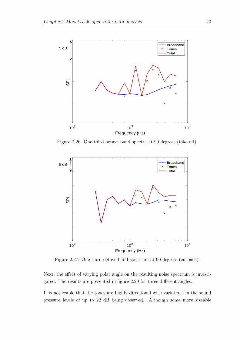
Chapter 2 Model scale open rotor data analysis 43
102 103 104
Frequency (Hz)
SP
L
BroadbandTonesTotal
5 dB
Figure 2.26: One-third octave band spectra at 90 degrees (take-off).
102 103 104
Frequency (Hz)
SP
L
BroadbandTonesTotal
5 dB
Figure 2.27: One-third octave band spectrum at 90 degrees (cutback).
Next, the effect of varying polar angle on the resulting noise spectrum is investi-
gated. The results are presented in figure 2.29 for three different angles.
It is noticeable that the tones are highly directional with variations in the sound
pressure levels of up to 22 dB being observed. Although some more sizeable
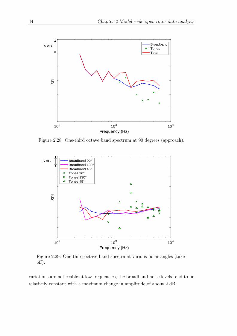
44 Chapter 2 Model scale open rotor data analysis
102 103 104
Frequency (Hz)
SP
L
BroadbandTonesTotal
5 dB
Figure 2.28: One-third octave band spectrum at 90 degrees (approach).
102 103 104
Frequency (Hz)
SP
L
Broadband 90°Broadband 130°Broadband 45°Tones 90°Tones 130°Tones 45°
5 dB
Figure 2.29: One third octave band spectra at various polar angles (take-off).
variations are noticeable at low frequencies, the broadband noise levels tend to be
relatively constant with a maximum change in amplitude of about 2 dB.

Chapter 2 Model scale open rotor data analysis 45
Comparison with tonal noise predictions
This section provides some examples of comparisons between Rig 145 measure-
ments and predictions calculated using currently available methods. The predic-
tions were performed using the current prediction tool used by Rolls-Royce. The
code was developed by M. Kingan (ISVR) and is based on the Landahl method
described by Parry. The prediction tool provides the tonal noise predictions for all
types of AOR noise sources, as well as calculations of the broadband noise com-
ponents. The tool also includes a model developed by Kingan and Sureshkumar
(Kingan et al. (2010), Kingan and Sureshkumar (2014)) which accounts for the
acoustic scattering of the tones from the centerbody of the AOR engine. Illustra-
tive results for a typical take-off case are shown in figures 2.30 and 2.31 for the
first rotor alone tone of the front rotor and the first interaction tone respectively.
These results were published by Kingan et al. (2014).
20 40 60 80 100 120 140 160Polar emission angle (°)
SP
L
1,0
Measured dataLoadingThicknessPredicted total
5 dB
Figure 2.30: Comparison with predictions - rig145.
The predictions show a reasonable agreement with the experimental data. As
expected, the loading noise is the principal source of rotor-alone tone noise, espe-
cially at take-off when the engine is highly loaded. The 1, 1 tone is essentially
dominated by the viscous wake interaction, although the forward potential (inter-
action of the front rotor blades with the rear rotor bound potential field) has a
significant contribution at some observer angles, as shown in figure 2.31.

46 Chapter 2 Model scale open rotor data analysis
40 60 80 100 120 140Polar emission angle (°)
SP
L
1,1
Measured data
Predicted total
Viscous wake
Rearward potential
Forward potential
Tip vortex
5 dB
Figure 2.31: Comparison with predictions - rig145.
2.4.2 Z08 rig tests
The analysis performed on the Z08 data is similar to that performed on the Rig 145
data. The polar directivity of tones and broadband noise, narrow band and one-
third octave band spectra for different rotational speeds, pitch and thrust settings
can be provided. The polar directivity patterns of rotor-alone and interaction
tones appear reasonable. Consequently, only a few illustrative examples are shown
in this section. An important feature of this analysis is that, whereas the Rig
145 measurements suffered from scattering by the C-shaped traverser, there was
no evidence of scattering effects in the measurements taken using the horizontal
traversing system (see figure 2.6) during the Z08 tests. Thus, it is believed that the
Z08 data will provide a high quality assessment of the noise field of an advanced
open rotor.
However, as for the Rig 145 data, the results for a particular tone displayed differ-
ences in the sound pressure levels measured by each microphone. Figures 2.32 and
2.34 show an illustration of the discrepancies between microphones for the polar
directivity patterns of a selection of tones. The continuous line and the errorbars
respectively show the median and the maximum and minimum values of sound
pressure level measured by all the microphones. The measurements from both
wire-mesh and flush mounted microphones are plotted separately.

Chapter 2 Model scale open rotor data analysis 47
40 60 80 100 120 140Polar emission angle (°)
SP
L
Wire−meshFlush mounted
5 dB
Figure 2.32: Polar directivity of the 1, 0 tone at take-off measured bywiremesh microphones - Z08.
0 20 40 60 80 100 120 140 160Polar emission angle (°)
SP
L
Wire−meshFlush mounted
5 dB
Figure 2.33: Polar directivity of the 1, 1 interaction tone at take-offmeasured by wiremesh microphones - Z08.
The results show a satisfactory agreement between the noise levels and directivity
patterns measured by the wire-mesh and the flush mounted microphones. The
median values of the range of data measured by the flush-mounted microphones
are over most of the frequency range within the measurement range of the wire-
mesh microphones.

48 Chapter 2 Model scale open rotor data analysis
20 40 60 80 100 120 140 160Polar emission angle (°)
SP
L
Wire−meshFlush mounted5 dB
Figure 2.34: Polar directivity of the 1, 2 interaction tone at take-offmeasured by wiremesh microphones - Z08.
Similar representation can be applied to compare the relative contributions of
broadband noise and tones for Z08 measurements. A one-third octave band spec-
trum for a typical take-off case, measured by the wire-mesh microphones, is shown
in figure 2.35. Differences in sound pressure levels up to 5 dB can be observed
within a one-third octave frequency band. It can be seen that the tones can be up
to 10 dB higher than the broadband noise levels.
Frequency
SP
L
BroadbandTonesTotal
1kHz
5 dB
Figure 2.35: One-third octave band spectra at 90 measured by wire-meshmicrophones (take-off).

Chapter 2 Model scale open rotor data analysis 49
2.5 Concluding remarks
The analysis of data collected during the Rig 145 and Z08 experimental test pro-
grammes provides polar directivity patterns of tones and broadband noise, as well
as narrow band and one-third octave band spectra at typical take-off, approach
and cutback cases. Preliminary comparisons show a good agreement with the cur-
rent analytical prediction model. The experimental results shown in this chapter
have been published by Kingan et al. (2014). The post-processing enables further
analysis of Rig 145 and Z08 data, to show the contribution from the different
sources of noise from the AORs. The analytical models presented in the following
sections will be compared with wind tunnel measurement data processed using the
methods described in this chapter.


Chapter 3
Loading noise produced by a
single rotor at angle of attack
3.1 Steady loading
The steady loading noise is caused by the component of the aerodynamic steady
forces exerted by the blades on the air. The prediction method presented here is
based on Hanson’s derivation of far-field loading noise produced by a propeller at
angle of attack (Hanson and Parzych, 1993) with a simplified blade geometry. The
starting point of Hanson and Parzych’s model is the acoustic analogy of Goldstein
(1974) which states that the acoustic density disturbance ρ′ at a location x at
time t in a moving medium with constant velocity in any volume ν bounded by
surfaces S in arbitrary motion is expressed as
c02ρ(x, t) =
∫ T
−T
∫S(τ)
ρ0V′nD0G
Dτ
dS(y)dτ
+
∫ T
−T
∫S(τ)
fi∂G
∂yidS(y)dτ +
∫ T
−T
∫ν(τ)
T ′ij∂2G
∂yi∂yjdydτ, (3.1)
where G is a Green’s function which satisfies the convected wave equation. The
source coordinates and time are respectively y = (y1, y2, y3) and τ . The first
term of this equation corresponds to the thickness noise where V ′n is given by
V ′n = Vn − ni.Ui with Ui = [U1, U2 = 0, U3 = 0]. The terms Vn and Ui are
51
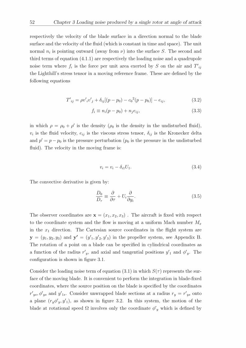
52 Chapter 3 Loading noise produced by a single rotor at angle of attack
respectively the velocity of the blade surface in a direction normal to the blade
surface and the velocity of the fluid (which is constant in time and space). The unit
normal ni is pointing outward (away from ν) into the surface S. The second and
third terms of equation (4.1.1) are respectively the loading noise and a quadrupole
noise term where fi is the force per unit area exerted by S on the air and T ′ij
the Lighthill’s stress tensor in a moving reference frame. These are defined by the
following equations
T ′ij = ρv′iv′j + δij[(p− p0)− c0
2(p− p0)]− eij, (3.2)
fi ≡ ni(p− p0) + njeij, (3.3)
in which ρ = ρ0 + ρ′ is the density (ρ0 is the density in the undisturbed fluid),
vi is the fluid velocity, eij is the viscous stress tensor, δij is the Kronecker delta
and p′ = p− p0 is the pressure perturbation (p0 is the pressure in the undisturbed
fluid). The velocity in the moving frame is:
vi = vi − δi1U1. (3.4)
The convective derivative is given by:
D0
Dτ
≡ ∂
∂τ+ Ui
∂
∂yi. (3.5)
The observer coordinates are x = (x1, x2, x3) . The aircraft is fixed with respect
to the coordinate system and the flow is moving at a uniform Mach number Mx
in the x1 direction. The Cartesian source coordinates in the flight system are
y = (y1, y2, y3) and y′ = (y′1, y′2, y′3) in the propeller system, see Appendix B.
The rotation of a point on a blade can be specified in cylindrical coordinates as
a function of the radius r′y, and axial and tangential positions y′1 and φ′y. The
configuration is shown in figure 3.1.
Consider the loading noise term of equation (3.1) in which S(τ) represents the sur-
face of the moving blade. It is convenient to perform the integration in blade-fixed
coordinates, where the source position on the blade is specified by the coordinates
r′ys, φ′ys and y′1s. Consider unwrapped blade sections at a radius ry = r′ys onto
a plane (ryφ′y, y′1), as shown in figure 3.2. In this system, the motion of the
blade at rotational speed Ω involves only the coordinate φ′y which is defined by

Chapter 3 Loading noise produced by a single rotor at angle of attack 53
Ω
y′1
x1, y1
y′3
x3, y3
γ
Mx
ryφ′y
y′3
y′2
Figure 3.1: Source coordinates in flight and propeller system.
φ′y = φ′ys + Ωτ . The force fi is a function of ry, φ′y and y′1 only, and the Green’s
function derivative is evaluated in terms of ry = r′ys, φ′y and y′1 = y′1s. The
surface S is no longer dependent on τ and the loading component can be written
pL(x, t) =
∫S
∫ T
−T
[fi(Ωτ)
∂G
∂yi
]φ′y=φ′ys+Ωτ
dτdS(y). (3.6)
Whereas Hanson expresses the locations of source area elements in terms of radial,
axial and tangential coordinates along the blade geometry, the present model uses
a flat plate approximation. The blade is assumed to be infinitely thin so the loading
forces are represented as net lift and drag forces per unit area acting normal to
the blade chordline and the integration is performed along the blade span and
chordwise coordinates. The blade is also assumed to be aligned with the local flow
direction. Note X the non dimensional chordwise coordinate normalized against
the half-chord
(X =
2X
c
). According to this approximation pL(x, t) is expressed
as
pL(x, t) ≈rt∫
rh
1∫−1
T∫−T
[Fi(Ωτ)
∂G
∂yi
]φ′y=φ′ys+Ωτ
dτc
2dXdry, (3.7)
where Fi is the lift and drag force per unit area acting on the blade chordline.
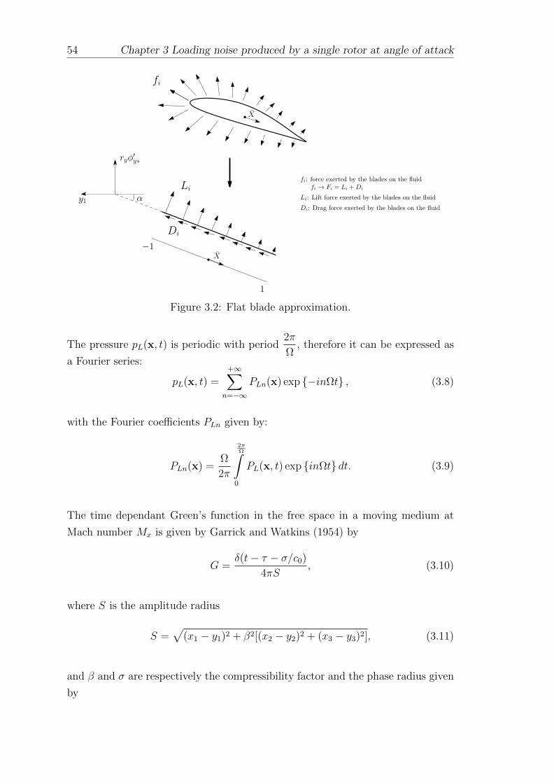
54 Chapter 3 Loading noise produced by a single rotor at angle of attack
fi
Di
Liα
ryφ′ys
y1
−1
1
X
X
fi: force exerted by the blades on the fluidfi → Fi = Li + Di
Di: Drag force exerted by the blades on the fluid
Li: Lift force exerted by the blades on the fluid
Figure 3.2: Flat blade approximation.
The pressure pL(x, t) is periodic with period2π
Ω, therefore it can be expressed as
a Fourier series:
pL(x, t) =+∞∑
n=−∞PLn(x) exp −inΩt , (3.8)
with the Fourier coefficients PLn given by:
PLn(x) =Ω
2π
2πΩ∫
0
PL(x, t) exp inΩt dt. (3.9)
The time dependant Green’s function in the free space in a moving medium at
Mach number Mx is given by Garrick and Watkins (1954) by
G =δ(t− τ − σ/c0)
4πS, (3.10)
where S is the amplitude radius
S =√
(x1 − y1)2 + β2[(x2 − y2)2 + (x3 − y3)2], (3.11)
and β and σ are respectively the compressibility factor and the phase radius given
by

Chapter 3 Loading noise produced by a single rotor at angle of attack 55
β =√
1−Mx2, (3.12)
σ =Mx(x1 − y1) + S
β2. (3.13)
Thus inserting the time dependant Green’s function from equation (3.10) into
equation (3.7) and using equation (3.9) yields
PLn(x) =Ω
2π
rt∫rh
1∫−1
T∫−T
[Fi(Ωτ)
∂
∂yi
δ(t− τ − σ/c0)
4πS
]φ′y=φ′ys+Ωτ
c
2dτdXdry. (3.14)
However, the limits of the integration over τ are indeterminate. To avoid this one
revolution of the rotor is considered, for example take values of τ between 0 and
2π/Ω, which corresponds to one period of the signal received from a time t1 to
t1 + 2π/Ω. So the noise pulse will be equal to pL(x, t) for t1 ≤ t < 2π/Ω and will
be zero outside this interval. Thus the following can be written
PLn(x) =Ω
2π
+∞∫−∞
PL(x, t) exp inΩt dt. (3.15)
Applying this in equations (3.14) gives
PLn(x) =Ω
2π
rt∫rh
1∫−1
2πΩ∫
0
[Fi(Ωτ)
∂
∂yi
(1
4πSexp
inΩ
σ
c0
)]φ′y=φ′ys+Ωτ
c
2dτdXdry.
(3.16)
The harmonic Green’s function is denoted by
Gn =exp inΩσ/c0
4πS. (3.17)
This leads to the following expression:

56 Chapter 3 Loading noise produced by a single rotor at angle of attack
PLn(x) =Ω
2π
rt∫rh
1∫−1
2πΩ∫
0
[Fi(Ωτ)
∂Gn
∂yi
]φ′y=φ′ys+Ωτ
exp inΩτ c2dτdXdry. (3.18)
The development of PL(x, t) deals with only one blade. For a propeller with B
blades it becomes
pLB(x) = pL(x, t)B−1∑q=0
exp i2πnq/B , (3.19)
where the sum over m equals the constant B if n/B ∈ Z and is equal to zero
elsewhere. This means that the sound will radiate only if n is a multiple of B.
Denote n = mB. Thus for a propeller with B equally spaced blades, each blade
encounters identical loading and radiates only at the blade passing frequencies
(n = mB). Equation (3.18) becomes
PLmB(x) =BΩ
2π
rt∫rh
12∫
−12
2πΩ∫
0
[Fi(Ωτ)
∂GmB
∂yi
]φ′y=φ′ys+Ωτ
exp imBΩτ c dτdXdry.
(3.20)
The lift force per unit area can be expressed as a Fourier series of the form
Fi(Ωτ) =+∞∑
k=−∞Fk exp −ikΩτ , (3.21)
Fk =Ω
2π
2πΩ∫
0
Fi(Ωτ) exp ikΩτ dτ. (3.22)
Inserting equation (3.21) into equation (3.20) and changing the variable of inte-
gration in the inner integral using φ′y = φys + Ωτ gives

Chapter 3 Loading noise produced by a single rotor at angle of attack 57
PLmB(x) =B
2π
rt∫rh
1∫−1
exp−i(mB − k)φ′ys
×2π∫
0
Fk∂GmB
∂yiexp
i(mB − k)φ′y
c2dφ′ydXdry. (3.23)
Far-field Green’s function in the emission coordinate system
In propeller noise studies, the emission (or retarded) coordinate system is often
used, cf. the conversion from reception to emission coordinates in Chapter 2. From
now, the far field Green’s function GmB will be evaluated in terms of retarded
coordinates. According to Hanson (1993) GmB can be written in this system
GmB =exp ikm(re − Scy′1)
4πS0
exp −ikmSsry cos(±φ′ − φy) , (3.24)
where re is the radiation distance to the observer from the emission point, and the
terms S0, Ss and Sc are given by
S0 = re(1−Mxcosθ), (3.25)
Sc =cos θ′
1−Mx cos θ, (3.26)
Ss =sin θ′
1−Mx cos θ, (3.27)
and km = mBΩ/c0 is the harmonic wavenumber. The notation θ′ corresponds to
the angle to the observer in retarded coordinates aligned with the propeller axis
and θ corresponds to the angle to the observer from the flight direction (see figure
3.3).
The partial derivatives fi∂GmB
∂yiin vector notation correspond to f.∇G which can
be evaluated in cylindrical coordinates as
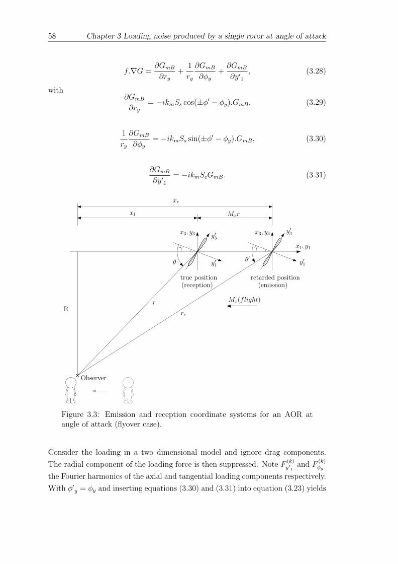
58 Chapter 3 Loading noise produced by a single rotor at angle of attack
f.∇G =∂GmB
∂ry+
1
ry
∂GmB
∂φy+∂GmB
∂y′1, (3.28)
with∂GmB
∂ry= −ikmSs cos(±φ′ − φy).GmB, (3.29)
1
ry
∂GmB
∂φy= −ikmSs sin(±φ′ − φy).GmB, (3.30)
∂GmB
∂y′1= −ikmScGmB. (3.31)
xr
Rre
Mxrx1
θ θ′
γ γ
y′3x3, y3
y′1
x1, y1
y′3x3, y3
retarded positiontrue position
Observer
Mx(flight)
y′1
(emission)(reception)
r
Figure 3.3: Emission and reception coordinate systems for an AOR atangle of attack (flyover case).
Consider the loading in a two dimensional model and ignore drag components.
The radial component of the loading force is then suppressed. Note F(k)y′1
and F(k)φy
the Fourier harmonics of the axial and tangential loading components respectively.
With φ′y = φy and inserting equations (3.30) and (3.31) into equation (3.23) yields

Chapter 3 Loading noise produced by a single rotor at angle of attack 59
PLmB(x) = −ikmBrt∫
rh
1∫−1
exp−i(mB − k)φ′ys
exp ikm(re − Scy′1)4πS0
×
1
2π
2π∫0
sin(±φ′ − φy) exp i(mB − k)φy exp −ikmSsry cos(±φ′ − φy) dφySsF (k)φ′y
+1
2π
2π∫0
exp imBφy exp −ikmSsry cos(±φ′ − φy) dφySsF (k)y′1
c2dXdry.
(3.32)
This expression can be written as
PLmB(x) = −ikmBexp ikmre
4πS0
rt∫rh
1∫−1
exp−i(mB − k)φ′ys
exp −ikmScy′1
× (SsIφyF(k)φy
+ ScIy1F(k)y′1
)c
2d(X)dry,
(3.33)
with
y′1 =c
2X cosα, (3.34)
φ′ys =c
2X
sinα
ry, (3.35)
and
Iφy =1
2π
2π∫0
sin(±φ′ − φ′ys) exp i(mB − k)φy exp −ikmSsry cos(±φ′ − φy) dφy,
(3.36)
Iy1 =1
2π
2π∫0
exp i(mB − k)φy exp −ikmSsr′y cos(±φ′ − φy) dφy. (3.37)

60 Chapter 3 Loading noise produced by a single rotor at angle of attack
The two components Iφy and Iy1 can be expressed as follows. Details for their
derivation are supplied in appendix A.
Iφy =mB − kkmSsry
expi(mB − k)(±φ′ − π
2)JmB−k(kmSsry), (3.38)
Iy1 = expi(mB − k)(±φ′ − π
2)JmB−k(kmSsry). (3.39)
The components of the loading force are given by
F(k)φy
= L cosα, (3.40)
F(k)y′1
= −L sinα, (3.41)
where L is the amplitude of the lift force acting on the blade per unit area defined
as a sum of a steady (L0) and an unsteady (Lk) component. Consider only the
steady component of the loading
L0 =1
2ρV (r′y)
2CL(r′y)f(X), (3.42)
where f(X) is a function describing the distribution of the lift forces along the
chord wise coordinate, CL is the lift coefficient and V the axial flow velocity. The
far-field steady loading noise of a propeller at angle of attack in a uniform flow is
finally given by:
PL(x, t) =+∞∑
m=−∞
−iB8πS0
exp
imB
(Ωt− re
c0
)+ i(mB − k)
(±φ′ − π
2
)
×rt∫
rh
1∫−1
exp
−i[(mB − k)
sinα
ry+ kmSc cosα
]cX
2
× c
2ρV (r′y)CL(r′y)f(X)
(mB − k
rycosα− kmSc sinα
)JmB−k(kmSsry) dXdry.
(3.43)

Chapter 3 Loading noise produced by a single rotor at angle of attack 61
3.2 Unsteady loading due to angle of attack
The present section comprises derivations of expressions to calculate the unsteady
lift on the airfoil produced by the periodic change in the angle of the airflow onto
each rotor blade as it rotates. In this formulation the blade sweep s is accounted
for by setting
y′1 =
(s+
cX
2
)cosα, (3.44)
φ′ys =
(s+
cX
2
)sinα
ry. (3.45)
The far-field pressure perturbation is thus
PL(x, t) =+∞∑
k=−∞
+∞∑m=−∞
−iB4πS0
exp
imB
(Ωt− re
c0
)+ i(mB − k)(±φ′ − π
2)
×rt∫
rh
ΨL exp −iΦs kyJmB−k(kmSsry)dry. (3.46)
with
kc =
(mBΩ cos θ′
c0(1−Mx cos θ)cosα + (mB − k)
sinα
ry
)c
2, (3.47)
ky =
((mB − k)
cosα
ry− mBΩ cos θ′
c0(1−Mx cosα)sinα
)c
2, (3.48)
Φs =
(mBΩ cos θ′
c0(1−Mx cos θ)cosα + (mB − k)
sinα
ry
)s, (3.49)
ΨL =
1∫−1
Lk exp−ikcX
dX. (3.50)
Blade lift calculation
The blade loading is calculated by estimating the upwash incident on each blade.
Note Ui and U ′i the axial flow velocity in the flight and propeller system respec-
tively.

62 Chapter 3 Loading noise produced by a single rotor at angle of attack
Figure 3.4: Flight and propeller coordinates.
The velocity in the propeller system is given by
U ′1 = U1 cos γ, (3.51)
U ′2 = −U1 sin γ, (3.52)
U ′3 = 0. (3.53)
α
r′yφ′y
y′1
X Ωr′y
Y
r′yφ′y
y′3
y′2
Ωr′y
Figure 3.5: Blade coordinates system.
The blade velocity and the air velocity relative to the observer in the propeller
system are respectively
VBO = Ωry[− sinφ′yy′2 + cosφ′yy
′3 ], (3.54)
VAO = U1 cos γy′1 − U1 sin γy′2.

Chapter 3 Loading noise produced by a single rotor at angle of attack 63
Thus the air velocity relative to the blade is
VAB = U1 cos γy′1 + [Ωry sinφ′y − U1 sin γ]y′2 − Ωry cosφ′yy′3. (3.55)
Figure 3.6: Coordinates system for velocity components.
The air velocity relative to the q = 0 blade in the axial, tangential and radial
directions are respectively
V ′1 = −U1 cos γ,
Vφ′y = − sinφ′yV′2 + cosφ′yV
′3 = −Ωry + U1 sin γ sin(Ωτ + φys),
Vr = 0. (3.56)
Therefore the flow velocities parallel and normal to the blade are given by the
following expressions (see figure 3.6).
VX = V ′1 cosα− Vφ′y sinα,
VY = −V ′1 sinα− Vφ′y cosα. (3.57)
As the blade is assumed to lie parallel to the time average flow, the stagger angle
α can be expressed (recall that φ′y = Ωτ + φ′ys)
64 Chapter 3 Loading noise produced by a single rotor at angle of attack
α = atan
(Ωry
U1 cos γ.
)(3.58)
The chordwise distribution of the steady component of lift force per unit area
acting on the rotor blade is calculated according to the expression of the pressure
distribution on a flat plate inclined at angle of incidence relatively to the airflow
given by the flat plate theory (Ashley and Landahl, 1965):
L0 =1
2ρVx
2CL
2
π
√1− X1 + X
. (3.59)
Therefore,
ΨL =1
2ρVx
2CL [J0 (kc) + iJ1 (kc)] , k = 0, (3.60)
where Vx is the steady component of flow parallel to the blade chordline. The
unsteady component of flow normal to the blade chordline is given by
νy = −U1 sin γ cosα sinφ′y. (3.61)
The upwash is defined as the sum of two gusts impinging on the flat airfoil such
that
νy =∑k′=±1
ν ′y exp ikX(VXτ −X) , (3.62)
where kX = k′Ω/VX and
ν ′y =i
2sgn(k′)U1 sin γ cosα exp −ikXs . (3.63)
At low frequency, the blade response to a gust of the form ν ′y exp ikX(VXτ −X)can be expressed using the compressible Sears’ response function as
∆p = 2ρVXν′ySc(σX)
√1− X1 + X
exp
ikXVXτ + i
¯σXMX2
β2X
, (3.64)
where σX = kXc
2and Sc(σX) is given by
Chapter 3 Loading noise produced by a single rotor at angle of attack 65
Sc(σX) =S(σX
β2 )
β
[J0
(MX
2σXβ2
)− iJ1
(MX
2σXβ2
)]exp
iσf(MX)
β2
, (3.65)
with
S
(σXβ2
)=
β2
iσX
[K0
(iσXβ2
)+K1
(iσXβ2
)] ,f(MX) = (1− β) ln(MX) + β ln(1 + β)− ln(2),
MX =VXc0
.
(3.66)
The above formulation is only valid in the low frequency regime, provided that
σXMX/β2 < 0.4. In the present application σXMX/β
2 < 0.1 for the first rotor
alone tone, hence the low frequency assumption is justified for the range of interest.
Assume that the unsteady component of the lift force per unit area L1 can be
expressed as a Fourier series of the form
Lk(ry, X, τ) =+∞∑
k=−∞lk(ry, X, k) exp ikΩτ , (3.67)
lk(ry, X, k) =Ω
2π
∫ 2πΩ
0
Lk(ry, X, τ) exp −ikΩτ dτ. (3.68)
According to equation (3.64) the unsteady loading per unit area is thus given by
Lk(ry, X, τ) =∑k′=±1
2ρVXν′ySc(σX)
√1− X1 + X
exp
ikXVXτ + i
σXMX2
β2X
(3.69)
Substituting into equation (3.50) and making use of the change of variables
X = cos θ/2, the chordwise distribution of the unsteady component of lift force
acting on the blade is
ΨL = πρVXν′ySc(σX)
[J0
(kc −
σXMX2
β2
)+ iJ1
(kc −
σXMX2
β2
)], k = ±1.
(3.70)

66 Chapter 3 Loading noise produced by a single rotor at angle of attack
3.3 Results
The model described in this Chapter has been validated internally against another
code developed by M. Kingan, based on the same method but written indepen-
dently (there is no available publication for this code). Comparisons with wind
tunnel measurements issued from Rig 145 test campaign are shown in figure 3.7
for the first rotor-alone tone of the upstream rotor at φ′ = 0. Predicted levels
were calculated for angles of attack in the range ±12 at a given emission radius.
The relative changes in sound pressure level produced by the changes in angle of
attack are well captured by the prediction method. Notice an increase in sound
pressure level with increase of the angle of attack, compared to the steady loading
case (black line), and vice versa. Those results were published and discussed in
great details in Kingan et al. (2014).
Figure 3.7: Polar directivity of the first rotor-alone tone for Rig 145 operat-ing at a condition representative of take-off (φ′ = 0). Measured SPL(left)predicted SPL (right).
3.4 Concluding remarks
An analytical model for predicting the loading noise produced by a propeller at
angle of attack was developed based on an existing method using a simplified blade
geometry. This model constitutes an improvement to the currently used model.
An extension to this work will be the derivation of a method to calculate the
thickness noise produced by a propeller at angle of attack.

Chapter 4
Interaction tone prediction
As mentioned in section 1.3, the rotor-rotor interaction tones can be caused by:
(1) the interaction of the front rotor’s wakes and tip vortices with the rear ro-
tor’s blades; (2) the interaction between the bound potential field of the front
(or rear) rotor with the adjacent blade row. Those tones are produced by the
unsteady forces caused by each of these flow distortions, and occur at frequencies
corresponding to the sum or difference of integer multiples of each rotor’s BPF,
i.e. if Ω and B denote the rotor’s rotational speed and blade number (with the
subscripts 1 and 2 corresponding to the front and rear rotor respectively), the
interaction tones would manifest at frequencies equal to
n1B1Ω1 + n2B2Ω2, n1 ∈ N, n2 ∈ N. (4.1)
The circumferential mode order of the tones is
ν = n1B1 − n2B2. (4.2)
In the present chapter far-field expressions to predict the rotor-rotor interaction
tones for an isolated AOR are derived, following the derivations of Hanson (1985b)
and Parry (1988). The blades are modelled as flat plates and are assumed to be
aligned with the flow direction. It is assumed that the noise is only produced by the
loading forces exerted by the blades on the fluid and the thickness and quadrupole
sources are neglected. For convenience the notations Xi, Yi and xi, yi are
used for the coordinate systems attached to each airfoil, where i = 1, 2. The
configuration of the two blade rows is shown in figure 4.1.
67

68 Chapter 4 Interaction tone prediction
X1Y1
x1 x2
Y2
X2α1
α2
y1 = ryφ1 y2 = ryφ2
ryΩ1
ryΩ2
g
2πryB2
2πryB1
Figure 4.1: Cascade representation of the front and rear rotor blades atconstant radius ry.
4.1 Downstream interactions
This section covers the noise produced by the interaction of the unsteady flow
field of the front rotor with the downstream rotor. The pressure perturbation at
location x and time t due to a rotor with B2 identical, evenly spaced blades is
given by
PL(x, t) =
B2−1∑q=0
∫ T
−T
∫∫S(q)
Fq.∇G(τ) dS(q)dτ, (4.3)
where Fq(τ) and G(τ) are respectively the force per unit area exerted by the fluid
on the qth blade’s surface S(q) and the free field Green’s function that can be
written as
G(τ) =1
2π
∫ +∞
−∞Gω′′ exp iω′′(t− τ) dω′′, (4.4)
and
Chapter 4 Interaction tone prediction 69
Fq(τ) =
∫ +∞
−∞Fq(ω
′) exp iω′τ dω′, (4.5)
Fq(ω′) =
1
2π
∫ +∞
−∞Fq(τ) exp −iω′τ dτ.
The times t and τ are respectively the observer time and the source time. Inserting
equations (4.4) and (4.6) in (4.3) yields
PL(x, t) =1
2π
B2−1∑q=0
T∫−T
∫∫S(q)
∫∫ +∞
−∞Fq(ω
′)Gω′′ exp iω′′(t− τ) + iω′τ dω′′dω′dX2drydτ.
(4.6)
The free-field Green’s function is given by (see Hanson)
Gω′′ =exp −iω′′σ/c0
4πS0
, (4.7)
where S0 and σ are the amplitude and phase radius defined, in the far-field, by
S0 = re(1−Mxcosθ), (4.8)
σ = re +xs cos θ
1−Mx cos θ− ry sin θ
1−Mx cos θcos(φ′ − φy). (4.9)
The quantity re corresponds to the distance from the source to the observer and
the coordinates (xs, ryφ′ys) correspond to the source coordinates with
φy = φ′ys + Ω2τ +2π
B2
q. (4.10)
The quantity φ′ys is the source’s azimuthal coordinate. Note that the axial co-
ordinate xs is defined in the opposite direction to Hanson’s notations. The force
Fq(ω′) can be decomposed in a sum of axial and tangential components relatively
to the blade stagger angle α2 as

70 Chapter 4 Interaction tone prediction
Fq(ω′) = xFx + φFφ = x sinα2Fq + φ cosα2Fq. (4.11)
The product Fq(ω′).∇Gω′′ can be evaluated in cylindrical coordinates as
Fq(ω′).∇Gω′′ = Fq(ω
′)
[sinα2
∂Gω′′
∂xs+
cosα2
ry
∂Gω′′
∂φy
], (4.12)
which gives the following result
Fq(ω′).∇Gω′′ =
iFq(ω′)ω′′ exp
−iω′′ σ
c0
4πS0c0(1−Mx cos θ)
[− cos θ sinα2 + sin θ cosα2 sin(φ′ − φy)] .(4.13)
Thus the pressure PL can be written
PL(x, t) =
B2−1∑q=0
T∫−T
∫∫S(q)
+∞∫∫−∞
iFq(ω′)ω′′
4πS0c0
exp
−iω
′′
c0
(re + Scxs)
× [− sinα2Sc + cosα2Ss sin(φ′ − φy)] exp iω′′(t− τ) + iω′τ
× exp
iω′′
c0
rySs cos(φ− φ0)
dω′′dω′dX2drydτ, (4.14)
with
Sc =cos θ′
1−Mx cos θ′, (4.15)
Ss =sin θ′
1−Mx cos θ′. (4.16)
Making use of the Jacobi-Anger formula yields

Chapter 4 Interaction tone prediction 71
PL(x, t) =
B2−1∑q=0
T∫−T
∫∫S(q)
+∞∫∫−∞
iFq(ω′)ω′′
8π2S0c0
exp
−iω
′′
c0
(re + Scxs)
× [− sinα2Sc + cosα2Ss sin(φ′ − φy)]+∞∑
n=−∞Jn
(ω′′rySsc0
)× exp
in(φ′ − φy +
π
2
)+ iω′′(t− τ) + iω′τ
dω′′dω′dX2drydτ.
(4.17)
The following product
sin(φ′ − φy)+∞∑
n=−∞Jn(z) exp
in(φ′ − φy +
π
2
)=
+∞∑n=−∞
∑j=±1
sgn(j)
2
× Jn(z) expi(n+ j)(φ′ − φy) + i(n− 1)
π
2
,
(4.18)
is equal to
−nz
expin(φ′ − φy +
π
2)Jn(z).
Thus, substituting φy for its definition in equation (4.10), performing the τ inte-
gration over infinity*,
∫ +∞
−∞exp −i(ω′′ − ω′ + nΩ2)τ dτ = 2πδ(ω′ − ω′′ − nΩ2), (4.19)
and integrating over ω′′, equation (4.17) can be written
PL(x, t) =
B2−1∑q=0
∫∫S(q)
∫ +∞
−∞
iFq(ω′)
4πS0
+∞∑n=−∞
exp
−iω
′ − nΩ2
c0
(re + Scxs)
×
[− sinα2Sc −
nc0 cosα2
ry(ω′ − nΩ2)
]ω′ − nΩ2
c0
Jn
((ω′ − nΩ2)rySs
c0
)× exp
i(ω′ − nΩ2)t+ in
(φ′ − φ′ys −
2πq
B2
+π
2
)dω′dXdry.
(4.20)

72 Chapter 4 Interaction tone prediction
Setting n = −n yields
PL(x, t) =
B2−1∑q=0
∫∫S(q)
∫ +∞
−∞
iFq(ω′)
4πS0
+∞∑n=−∞
exp
−iω
′ + nΩ2
c0
(re + Scxs)
×
[− sinα2Sc +
nc0 cosα2
ry(ω′ + nΩ2)
]ω′ + nΩ2
c0
(−1)nJn
((ω′ + nΩ2)rySs
c0
)× exp
i(ω′ + nΩ2)t− in
(φ′ − φ′ys −
2πq
B2
+π
2
)dω′dX2dry.
(4.21)
The force acting on the rear rotor blade is periodic with period T =2π
B1(Ω1 + Ω2)
thus Fq(ω′) can be expressed as a sum of impulses as
Fq(ω′) =
+∞∑k=−∞
Fkδ (ω′ − kB1(Ω1 + Ω2)) , (4.22)
where Fk is the harmonic of the unsteady lift force per unit area. Thus substituting
equation (4.22) into equation (4.21) and integrating over ω′ yields
PL(x, t) =
B2−1∑q=0
∫∫S(q)
+∞∑k=−∞
+∞∑n=−∞
(−1)niFk
4πS0
exp
−i(kB1(Ω1 + Ω2) + nΩ2)(re + Scxs)
c0
× kB1(Ω1 + Ω2) + nΩ2
c0
[− sinα2Sc +
nc0 cosα2
ry(kB1(Ω1 + Ω2) + nΩ2)
]× Jn
((kB1(Ω1 + Ω2) + nΩ2)rySs
c0
)exp i(kB1(Ω1 + Ω2) + nΩ2)t
× exp
−in
(φ′ − φ′ys −
2πq
B2
+π
2
)dX2dry. (4.23)
Setting n = n− kB1 yields

Chapter 4 Interaction tone prediction 73
PL(x, t) =
B2−1∑q=0
∫∫S(q)
+∞∑k=−∞
+∞∑n=−∞
iFk4πS0
exp
−i(kB1Ω1 + nΩ2)
re + Scxsc0
kB1Ω1 + nΩ2
c0
× (−1)n−kB1
[− sinα2Sc +
(n− kB1)c0 cosα2
ry(kB1Ω1 + nΩ2)
]Jn−kB1
((kB1Ω1 + nΩ2)rySs
c0
)× exp
i(kB1Ω1 + nΩ2)t− i(n− kB1)
(φ′ − φ′ys −
2πq
B2
+π
2
)dX2dry.
(4.24)
The unsteady lift harmonic Fk can be written
Fk = F0 exp
ikB1
2πq
B2
, (4.25)
Thus
PL(x, t) =
B2−1∑q=0
∫∫S(q)
+∞∑k=−∞
+∞∑n=−∞
iF0
4πS0
exp
−i(kB1Ω1 + nΩ2)
re + Scxsc0
kB1Ω1 + nΩ2
c0
× (−1)n−kB1
[− sinα2Sc +
(n− kB1)c0 cosα2
ry(kB1Ω1 + nΩ2)
]Jn−kB1
((kB1Ω1 + nΩ2)rySs
c0
)× exp
i(kB1Ω1 + nΩ2)t− i(n− kB1)
(φ′ − φ′ys +
π
2
)+ in
2πq
B2
dX2dry.
(4.26)
The sum
B2−1∑q=0
exp
i2πnq
B2
is equal to the constant B2 if n/B2 ∈ Z and is equal
to zero elsewhere. We note n = mB2 where m is an integer. Thus equation (4.27)
becomes
PL(x, t) =
∫∫S(q)
+∞∑k=−∞
+∞∑m=−∞
iB2F0
4πS0
exp
−iωre + Scxs
c0
ω
c0
(−1)ν
×[− sinα2Sc +
νc0 cosα2
ryω
]Jν
(ωrySsc0
)× exp
iωt− i(mB2 − kB1)
(φ′ − φ′ys +
π
2
)dX2dry, (4.27)
where ω = kB1Ω1 +mB2Ω2 and ν = mB2− kB1 . The above equation is equal to

74 Chapter 4 Interaction tone prediction
PL(x, t) =
∫∫S(q)
+∞∑k=−∞
+∞∑m=−∞
iB2F0
4πS0
exp
iω
(t− re + Scxs
c0
)exp
−iν
(φ′ − φ′ys
)× exp
−iν π
2
[−ω sinα2
Scc0
+ν cosα2
ry
]J−ν
(ωrySsc0
)dX2dry. (4.28)
The axial and tangential source coordinates are given by
xs = (s2 +X2) cosα2 + (l2 + Y2) sinα2, (4.29)
φ′ys = −(s2 +X2)sinα2
ry+ (l2 + Y2)
cosα2
ry,
where s2 and l2 are respectively the sweep and lean of the downstream airfoil.
x2
Y2
X2
α2
y2
(x0, r0φs)
s
l
Figure 4.2: Blade sweep and lean definition.
Note that on the blade surface, Y2 = 0. We denote m = n2 and k = n1. Insert-
ing equation (4.30) into equation (4.28) and using the non-dimensional chordwise
coordinate X2 =2X2
c2
yields
PL(x, t) =iB2
4πS0
rt2∫rh2
+∞∑n1=−∞
+∞∑n2=−∞
exp
i(n2Ω2 + n1Ω1)
(t− re
c0
)
× exp−i(n2B2 − n1B1)
(φ′ +
π
2
)exp −iΦs − ikY ll
× kY lJn1B1−n2B2
(ωrySsc0
)ΨL dry, (4.30)
where ΨL is the ”acoustically weighted” lift per unit span which is defined as
Chapter 4 Interaction tone prediction 75
ΨL =
∫ 1
−1
F0 exp−ikXsX2
dX2, (4.31)
and the wave numbers kXs and kY l are given by
kXs =c2
2
[ωScc0
cosα2 + (n2B2 − n1B1)sinα2
ry
](4.32)
kY l =c2
2
[ωScc0
sinα2 − (n2B2 − n1B1)cosα2
ry
]. (4.33)
Φs = s2
[ωScc0
cosα2 + (n2B2 − n1B1)sinα2
ry
]. (4.34)
4.2 Upstream interactions
Now consider the noise produced by the interaction between the disturbed flow
field of the downstream rotor and the upstream blade row. The derivation is
identical to that of section 4.1, expressing the force exerted by the upstream blades
on the flow as follows.
Fq(ω′) = −xFq sinα1 + φ cosα1Fq. (4.35)
Hence, the acoustic pressure perturbation is given by
PL(x, t) =iB1
4πS0
rt1∫rh1
+∞∑n1=−∞
+∞∑n2=−∞
exp
i(n2Ω2 + n1Ω1)
(t− re
c0
)
× exp−i(n1B1 − n2B2)
(φ′ +
π
2
)exp −iΦs − ikY ll
× kY lJn2B2−n1B1
(ωrySsc0
)ΨL dry, (4.36)
with the wave numbers kXs and kY l given by
76 Chapter 4 Interaction tone prediction
kXs =c1
2
[ωScc0
cosα1 + (n2B2 − n1B1)sinα1
ry
](4.37)
kY l =c1
2
[ωScc0
sinα1 + (n2B2 − n1B1)cosα1
ry
]. (4.38)
and
Φs = s1
[ωScc0
cosα1 + (n2B2 − n1B1)sinα1
ry
], (4.39)
ΨL =
∫ 1
−1
F0 exp−ikXsX1
dX1. (4.40)
4.3 Concluding remarks
Far-field expressions for predicting the rotor-rotor interaction tones produced by
an isolated advanced open rotor were derived based on existing methods. Those
expressions will be used in the following chapter to calculate the far-field. The
formulation of the downstream interactions given by equation (4.30) will be used
to calculate the noise produced by: (1) the impingement of the front rotor viscous
wakes onto the downstream rotor in Chapter 5; (2) the interaction of the potential
field of the upstream rotor with the downstream rotor in Chapter 6. Formulation
(4.36) will be used to calculate the noise produced by the interaction between the
potential field of the downstream rotor with the upstream blade row.

Chapter 5
Wake interaction noise
5.1 Introduction
The wake interaction is a dominant source of interaction noise for an advanced
open rotor. Predicting wake interaction noise requires the knowledge of the aerody-
namic properties of the flow around the blades. These parameters can significantly
influence the resulting sound pressure levels, thus the input of high fidelity aerody-
namic data into the analytical models is essential. Calculating such accurate data
is critical as the flow field around the blades is unsteady and complex, however
some meticulous unsteady CFD simulations can improve the agreement between
predictions and experimental data (Kingan et al. (2014), Carazo et al. (2011)).
Another alternative is the use of experimental methods to capture the features of
the distorted flow field around the blades (Santana et al. (2013), Sinnige et al.
(2015)). Previous work by Kingan et al. (2014) investigated the prediction of
the far field noise produced by an advanced open rotor using a method in which
the steady aerodynamics of the rotor were predicted using both steady CFD and
a strip method. The steady aerodynamics of the front rotor were input into a
purely analytical model which predicted the unsteady flow field produced by the
front rotor, the unsteady response of the downstream blade, and the radiated
far-field tonal noise. It was suggested that the accuracy of the method relied on
an accurate representation of the steady aerodynamics of the rotor namely, that
obtained from high fidelity three-dimensional CFD. However, the accuracy of the
method also relied on the ability of the analytical models to accurately predict
the rotor wake development using this steady aerodynamic data. In this chapter,
the ability of such analytical methods to accurately model the development of the
77

78 Chapter 5 Wake interaction noise
front rotor wakes is assessed using a hybrid CFD/analytical method. This work
was published by Ekoule et al. (2015).
5.2 Hybrid CFD/analytical model
5.2.1 Method
The present method is inspired from the work of Carazo et al. (2011) who used
URANS CFD data to model the incident flow field at the rear rotor leading edge.
The numerical data were then input into analytical models to calculate the blade
response and the far-field radiated noise. Because the development of the wakes
provided by such simulations can be subject to numerical dissipation, analytical
methods for modelling the evolution of the viscous wakes are still of interest. In
the present model, the wake characteristics such as wake width and wake centerline
velocity are determined from high fidelity unsteady three-dimensional CFD data
collected at a particular axial plane and an analytical model is used to convect
the wakes to downstream locations. A similar approach was followed by Jaron
et al. (2014), who used another analytical model to determine the front rotor
wake and potential field upstream of the rear rotor from RANS measurements
taken at upstream locations.
The CFD simulations used in this method were supplied by N.Sohoni from the Uni-
versity of Cambridge’s Rolls-Royce University Technology Centre. Subsequently
the author appraised the simulation data and post-processed ‘raw’ instantaneous
velocity data. The simulations were performed using Turbostream (Brandvik and
Pullan, 2011), which is a fast, three-dimensional, Unsteady Reynolds-Averaged
Navier-Stokes (URANS) solver running on structured multi-block meshes. Tur-
bostream uses an algorithm based on the TBLOCK solver, a code originally devel-
oped by Denton (1983). The numerical scheme is a finite-volume method, second-
order accurate in time and space. The CFD simulations used structured multiblock
meshes with an O-mesh surrounding each blade. The domains of each rotor were
connected by a sliding surface using polynomial interpolation in the circumfer-
ential direction. The mesh topology is shown in figure 5.1 whereNθF
ZFand
NθR
ZRcorrespond to the number of circumferential grid points per blade pitch at the
upstream and downstream blocks respectively. The data analyzed in this Chap-
ter were captured at various locations upstream and downstream of the sliding
surface. The rotor geometry used in the simulations were taken from open rotor

Chapter 5 Wake interaction noise 79
blades designed by Rolls-Royce and tested on Airbus Z08 test rig (note that the
Z08 test rig is described in Chapter 2).
Figure 5.1: Blade-to-blade mesh topology, originally published by Sohoniet al. (2015). S and ε correspond to pitch and thickness quantities.
The model assumes that the stream tube contraction is small downstream of the
location at which the data is collected such that the wake profile measured at a
particular radial location convects downstream of this point at a constant radius.
The validity of this assumption may be assessed by inspection of figure 5.2 which
plots the instantaneous velocity components and instantaneous velocity magnitude
in a meridional plane. It is observed that, apart from very close to the front
rotor blades, the radial component of velocity is significantly less than the axial
component of velocity in the region between the two rotors. This should ensure
that fluid particles propagate along a path which has an approximately constant
radius.
(a) (b)
Figure 5.2: Contours of constant instantaneous velocity in a meridionalplane: (a) axial velocity, (b), radial velocity. The color scaling limitVmax corresponds to the maximum absolute velocity magnitude across themeridional plane and Vmin ≈ −0.7Vmax.

80 Chapter 5 Wake interaction noise
5.2.2 Coordinate system
Consider the coordinate system X1, Y1 which rotates with the ‘reference wake’
of the front rotor ‘reference blade’, for which the coordinates X1 and Y1 are,
respectively, tangent and normal to the mean flow direction in a frame of reference
rotating with the front rotor at a particular radius. The x1, y1 coordinate system
also rotates with the front rotor with x1 parallel to the rotor axis and y1 = rφ1
parallel to the tangential direction. The deficit velocity due to the viscous wake
from each blade on the front rotor is assumed to be identical and aligned with the
mean flow direction at the measurement plane. The origin of the X1, Y1 and
x1, y1 coordinate systems is selected to be located at the same axial position as
the trailing edge of the front rotor blades. Note that in the method described by
Parry (1988), the origin of this coordinate system was placed at the mid chord of
the front rotor blade. The X1, Y1 and x1, y1 coordinate systems are related
by
X1 = x1 cosα1 + y1 sinα1, (5.1)
Y1 = −x1 sinα1 + y1 cosα1, (5.2)
where α1 is the local flow angle. The coordinates are shown in figure 5.3.
X1Y1
x1 x2
Y2
X2α1
α2
y1 y2Ω1
Ω2
g
Figure 5.3: Cascade coordinate system.

Chapter 5 Wake interaction noise 81
5.2.3 Wake velocity profile
The analytical model assumes that, at each radius, the wake can be modelled as
two-dimensional and propagates in the mean flow direction which is modelled as
constant in the inter-rotor region. Finally, the wakes of the front rotor are assumed
to be far enough from each other to be considered as isolated wakes. In fact, in
the present configuration the solidity is low enough for the cascade effects to be
ignored (s/c1 & 1, where s/c1 is the pitch/chord ratio), see Blandeau et al. (2011).
The wake velocity deficit is modeled by a Gaussian function whose variables were
determined from data at a measurement plane, P1, which is located at a constant
axial location 0.0902D1 (where D1 is the diameter of the front rotor) downstream
of the front rotor blade pitch change axis, see figure 5.4. Figure 5.5 shows contours
of constant tangential velocity calculated from the CFD simulation for one front
rotor blade passage at this particular plane. It is assumed that the velocity field
at the measurement plane can be modeled as a linear sum of the velocity produced
by the front and rear rotors.
P1
sliding plane
Figure 5.4: Location of the plane P1.
Thus, in the frame of reference of the front rotor, the flow disturbances due to
the front rotor are steady in time and the perturbations due to the rear rotor are
fluctuating with time. As described by Carazo et al. (2011), a time average of the
velocity at the measurement plane in a frame of reference moving with the front
rotor, will remove the unsteady portion of the flow due to the rear rotor leaving
only the steady component of the flow and the unsteady components associated
with the front rotor. The instantaneous and time-averaged tangential velocity at
80% of the tip radius are plotted as a function of φ1, an azimuthal angle which
rotates with the front rotor, in Figure 5.6.
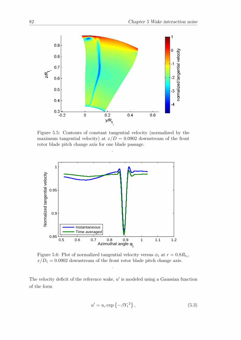
82 Chapter 5 Wake interaction noise
Figure 5.5: Contours of constant tangential velocity (normalized by themaximum tangential velocity) at x/D = 0.0902 downstream of the frontrotor blade pitch change axis for one blade passage.
.
0.5 0.6 0.7 0.8 0.9 1 1.1 1.20.85
0.9
0.95
1
Azimuthal angle φ1
Nor
mal
ized
tang
entia
l vel
ocity
Instantaneous Time averaged
Figure 5.6: Plot of normalized tangential velocity versus φ1 at r = 0.8Rt1 ,x/D1 = 0.0902 downstream of the front rotor blade pitch change axis.
.
The velocity deficit of the reference wake, u′ is modeled using a Gaussian function
of the form
u′ = uc exp−βY1
2, (5.3)

Chapter 5 Wake interaction noise 83
where the wake centerline deficit velocity uc and the parameter β are determined
from the CFD data on the measurement plane by matching the centerline velocity
and momentum deficit of the analytic and CFD velocity profiles. The method is
described in details in Appendix C. As a result, the relationship between β and
uc is given by
β = π
(uc
(−2 +
uc√
2
Ur
)ρ0Ur
dD/dr 2 cosα1
)2
, (5.4)
where ρ0 is the air density and dD/dr is the drag force per unit span. Figure 5.7
shows the wake velocity deficit normalized against the mean velocity Ur at radius
r = 0.8Rt1 (where Rt1 is the tip radius of the front rotor) for both the analytic
model and the CFD data at the measurement plane. The principal features of the
wake are reproduced with a reasonably good agreement with the CFD wake profile.
The additional velocity components at the edges of the wake will be subject to
further investigations. It is assumed that the fluctuations in the velocity deficit
outside the viscous wake region are primarily due to the bound potential field of
the front rotor. This contribution is investigated in Chapter 6.
−0.2 −0.15 −0.1 −0.05 0 0.05 0.1 0.15
−0.12
−0.1
−0.08
−0.06
−0.04
−0.02
0
Nor
mal
ized
vel
ocity
def
icit
u’/U
r
Y1/R
t1
CFDAnalytical model
Figure 5.7: Normalized wake velocity deficit at radius r = 0.8Rt1 . Compar-ison between the analytical model and the CFD data at the measurementplane.
.
In figure 5.8, the tangential velocity profiles given by the CFD and those calculated
using the analytical method over the entire (r, θ) measurement plane are compared.

84 Chapter 5 Wake interaction noise
In this plane, there is clearly good qualitative agreement between the CFD and
the Gaussian models of the viscous wake. Nevertheless one source of discrepancy
is the tip vortex which is noticeable in the full CFD solution but which is not
included in the analytical model.
(a)
(b)
Figure 5.8: Tangential velocity at the plane P1 normalized by the frontrotor tip speed given by the CFD data (a) and the analytical model (b).
To assess the development of the wake along the axial coordinate and to calculate
the upwash incident on the surface of the downstream blade, the wakes are con-
vected downstream following a scaling law deduced from the analytical expressions
of uc and β given by Eq. (5.2.31) and (5.2.40) in Parry (1988)
β ∝ 1
X ′1, (5.5)
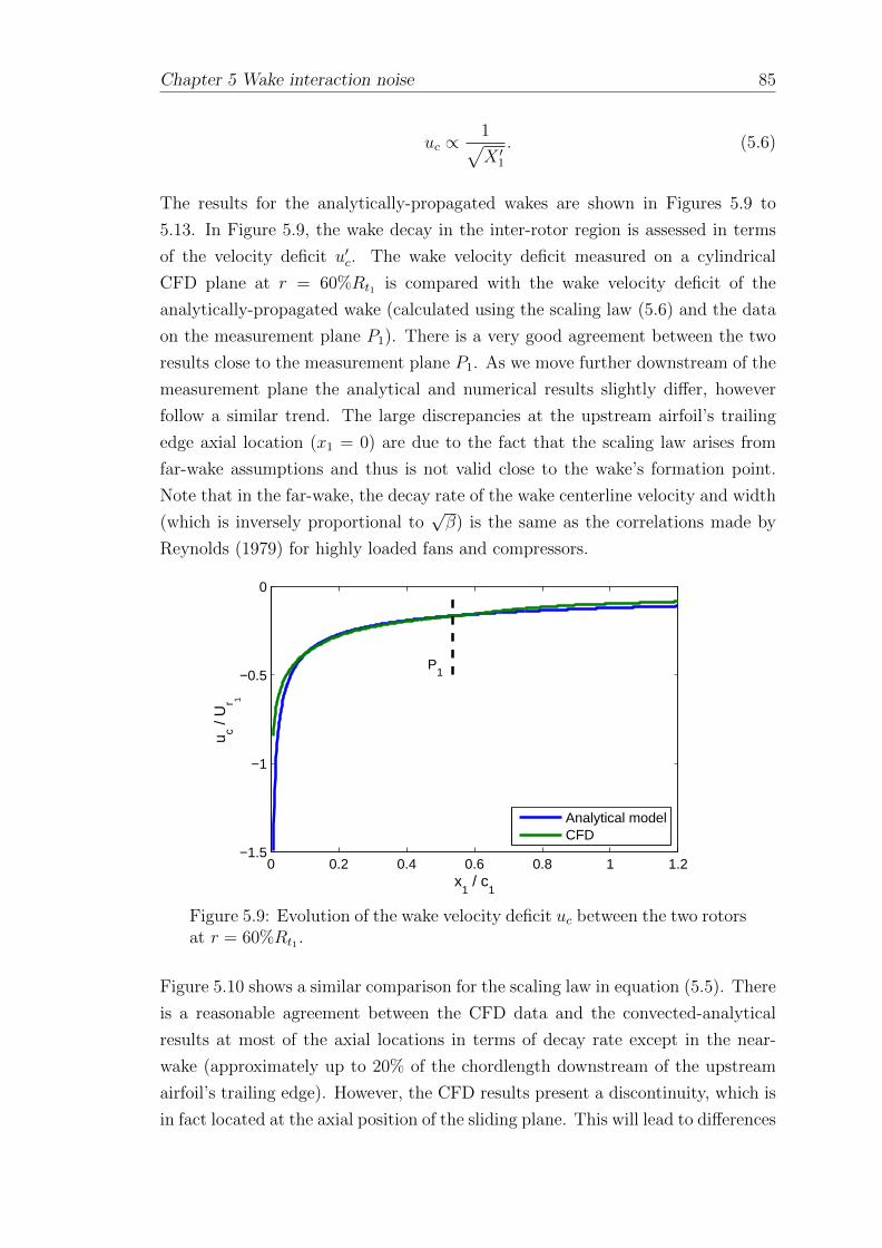
Chapter 5 Wake interaction noise 85
uc ∝1√X ′1
. (5.6)
The results for the analytically-propagated wakes are shown in Figures 5.9 to
5.13. In Figure 5.9, the wake decay in the inter-rotor region is assessed in terms
of the velocity deficit u′c. The wake velocity deficit measured on a cylindrical
CFD plane at r = 60%Rt1 is compared with the wake velocity deficit of the
analytically-propagated wake (calculated using the scaling law (5.6) and the data
on the measurement plane P1). There is a very good agreement between the two
results close to the measurement plane P1. As we move further downstream of the
measurement plane the analytical and numerical results slightly differ, however
follow a similar trend. The large discrepancies at the upstream airfoil’s trailing
edge axial location (x1 = 0) are due to the fact that the scaling law arises from
far-wake assumptions and thus is not valid close to the wake’s formation point.
Note that in the far-wake, the decay rate of the wake centerline velocity and width
(which is inversely proportional to√β) is the same as the correlations made by
Reynolds (1979) for highly loaded fans and compressors.
0 0.2 0.4 0.6 0.8 1 1.2−1.5
−1
−0.5
0
u c / U
r 1
x1 / c
1
Analytical modelCFD
P1
Figure 5.9: Evolution of the wake velocity deficit uc between the two rotorsat r = 60%Rt1 .
Figure 5.10 shows a similar comparison for the scaling law in equation (5.5). There
is a reasonable agreement between the CFD data and the convected-analytical
results at most of the axial locations in terms of decay rate except in the near-
wake (approximately up to 20% of the chordlength downstream of the upstream
airfoil’s trailing edge). However, the CFD results present a discontinuity, which is
in fact located at the axial position of the sliding plane. This will lead to differences
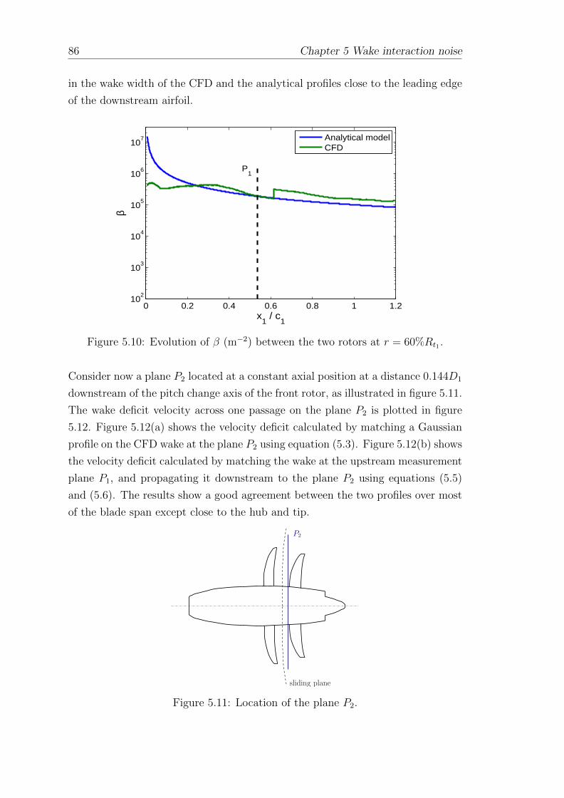
86 Chapter 5 Wake interaction noise
in the wake width of the CFD and the analytical profiles close to the leading edge
of the downstream airfoil.
0 0.2 0.4 0.6 0.8 1 1.210
2
103
104
105
106
107
x1 / c
1
β
Analytical modelCFD
P1
Figure 5.10: Evolution of β (m−2) between the two rotors at r = 60%Rt1 .
Consider now a plane P2 located at a constant axial position at a distance 0.144D1
downstream of the pitch change axis of the front rotor, as illustrated in figure 5.11.
The wake deficit velocity across one passage on the plane P2 is plotted in figure
5.12. Figure 5.12(a) shows the velocity deficit calculated by matching a Gaussian
profile on the CFD wake at the plane P2 using equation (5.3). Figure 5.12(b) shows
the velocity deficit calculated by matching the wake at the upstream measurement
plane P1, and propagating it downstream to the plane P2 using equations (5.5)
and (5.6). The results show a good agreement between the two profiles over most
of the blade span except close to the hub and tip.
sliding plane
P2
Figure 5.11: Location of the plane P2.

Chapter 5 Wake interaction noise 87
For this particular case, there is very good agreement between the profiles at radial
locations between 75% and 85% of the front rotor tip radius. Figure 5.13 shows
a comparison between the data from figures 5.12(a) and 5.12(b) at approximately
a radius of 80% of the front rotor tip radius. There is remarkably good agree-
ment between the two, particularly being cognizant of the fact that no streamtube
contraction effects or radial flow effects have been included in the model.
(a)
(b)
Figure 5.12: Normalized wake deficit, at a distance 0.144D1 downstreamof the front rotor pitch change axis calculated by (a) fitting a Gaussianprofile to the CFD data in this plane, (b) using the data collected at theoriginal measurement plane and propagating the wakes downstream usingthe scaling laws (5.5) and (5.6).
However, some of the discrepancies between the analytical and the numerical result
show some important features. In accordance with figure 5.10, slightly larger wakes
are observed up to around 60% of the front rotor tip radius. This is in part due to

88 Chapter 5 Wake interaction noise
the presence of acceleration regions at the edges of the CFD wake as well as the
discontinuity previously observed at the sliding plane.
0.4 0.5 0.6 0.7 0.8 0.9 1 1.1−0.12
−0.1
−0.08
−0.06
−0.04
−0.02
0
0.02
Azimuthal angle φ1
Nor
mal
ized
vel
ocity
def
icit
u’/U
r 1
CFDAnalytical − convected wakeAnalytical − fitted wake
Figure 5.13: Normalized wake velocity deficit at the plane P2 at r ≈ 0.8Rt1 .The term Ur1 is the mean velocity magnitude at this location.
At some radii, a difference is observed in the angular position of the wake cen-
terline, which engenders a difference in the relative phases between the sources
of both models at each spanwise location. This would result in a different treat-
ment of interferences in the calculation of the sound radiation. A preliminary
investigation of those disparities showed that those angular shifts correspond to a
variation of distance to the leading edge in the chordwise direction of up to 6% of
the chordlength (on average, the difference is approximately 1.4%) and differences
in phase of up to 2.6% (1% on average). As a result, this contributed to a differ-
ence of 1-3dB in the radiated noise levels at particular angles and frequencies, but
it had little effect on the directivity pattern of the considered tones. Yet, further
investigation of those disparities is required to assess their importance in greater
details.
We now wish to propagate the reference wake velocity deficit from P1 to a curved
surface at the location of the leading edge of the downstream rotor and to calculate
the upwash incident on it. It is assumed that in the vicinity of this location the
wake profile develops only very slowly in the axial direction (thus β and uc can
be regarded as being constant at axial locations close to the axial position of the
leading edge of the downstream rotor blades). Due to the periodicity of the front

Chapter 5 Wake interaction noise 89
rotor wake profiles in the tangential direction, the velocity deficit incident on the
rear rotor blades can be decomposed as a Fourier series:
u (r, φ1) =+∞∑
n1=−∞un1 exp in1B1φ1 , (5.7)
with
un1 =B1
2π
∫ φc+πB1
φc− πB1
u(r, φ1) exp −in1B1φ1 dφ1 (5.8)
and φc is the value of φ1 at the wake centerline at the axial location of the rear rotor
blades. Substituting equations (5.2) and (5.3) into equation (5.8) and evaluating
the integral yields
un1 = (cosα1, sinα1)ucB1
2r cosα1
√πβ
exp
−in1B1x1
tanα1
r
exp
−(
n1B1
2rcosα1
√β
)2.
(5.9)
The upwash on the qth blade of the downstream rotor can be rewritten in the
x2(q), y2
(q)coordinate system which rotates with the downstream blade row and
which is related to the x1, y1 coordinate system by the following equations.
x1 = x2(q) + g +
(s2 −
c2
2cosα2 + l2 sinα2
), (5.10)
y1 = y2(q) +
2πrq
B2
+ (Ω1 + Ω2)rt−(s2 −
c2
2sinα2 + l2 cosα2
), (5.11)
where g is the axial distance between x1 = 0 and the pitch change axis of the
downstream rotor, α2 is the stagger angle of the rear rotor blades and s2 and l2
are, respectively, the rear rotor blade sweep and lean. It is also convenient to
define a downstream blade coordinate system, X2(q), Y2
(q) which is related to
the coordinate system x2(q), y2
(q) by
x2(q) = X2
(q) cosα2 + Y2(q) sinα2, (5.12)
y2(q) = −X2
(q) sinα2 + Y2(q) cosα2.

90 Chapter 5 Wake interaction noise
The incident upwash normal to the qth downstream blade, v′, is thus given by
v′ =+∞∑
n1=−∞Vn1 exp
ikX(Ur2t−X2
(q))− ikY Y2(q) + in1B1
2πq
B2
, (5.13)
where
Vn1 =sin(α1 + α2)ucB1
2r cosα1
√βπ
exp
−(
n1B1
2r cosα1
√β
)2
× exp
−ikX
(s2 −
c2
2
)− ikY l2 − in1B1
tanα1
rg
, (5.14)
kX =n1B1
r cosα1
sin(α1 + α2), (5.15)
kY = − n1B1
r cosα1
cos(α1 + α2), (5.16)
Figure 5.14 shows the magnitude of the upwash harmonics calculated at one par-
ticular radial location at the rear rotor inlet. The upwash velocity for one blade
passage is shown in figure 5.14 (a) and the Fourier harmonics are shown in figure
5.14 (b) (the case n1 = 0 is not considered here since it does not affect the noise
field). It is of particular interest to note that, although the spatial velocity fields
from the CFD are well-replicated by the model, the Fourier components show
some disagreements for a number of harmonics. These disagreements are clearly
influenced by the flow regions at the edge of the wake and these regions contain
contributions from velocity fields other than just that of the viscous wake. In fact,
the averaging process used in this method may not perfectly isolate the viscous
wake thus additional flow components may have been preserved. Consequently,
there are likely to be associated errors in the predictions of the interaction tones
which are, of course, driven by all the unsteady velocity fields.

Chapter 5 Wake interaction noise 91
(a)
0.4 0.5 0.6 0.7 0.8 0.9 1 1.1−0.1
−0.08
−0.06
−0.04
−0.02
0
0.02
Azimuthal angle φ1
Nor
mal
ized
upw
ash
velo
city
v’/U
r 1
CFDAnalytical model − convected wake
(b)
0 5 10 15 20 25 30n
1
|Un 1|
CFDAnalytical model − convected wake
Figure 5.14: Normalized upwash velocity at the rear rotor inlet plane(r ≈ 0.8Rt1): (a) velocity magnitude, (b) Fourier harmonics.

92 Chapter 5 Wake interaction noise
5.2.4 Airfoil response
In the present case, only the high frequency regime is considered since the reduced
frequency is relatively high for the interaction tones of interest. Thus the acoustic
wavelength is sufficiently smaller than the chord so that leading edge noise sources
can be decoupled from the trailing edge. Since in the case of wake-interaction
most of the loading is concentrated at the downstream blade leading edge, only
the latter is considered, the trailing edge contribution being small at high fre-
quency. The downstream airfoil is thus modeled as a semi-infinite plate extending
to downstream infinity. The validity of this assumption is discussed at the end of
this section. The response of the downstream rotor blade to the incident upwash is
calculated using standard two-dimensional unsteady airfoil theory, as described in
Goldstein (1974) and Parry (1988), for the high frequency response of an aerofoil
to a harmonic convected gust in compressible flow. The total unsteady lift per
unit area acting on the planform of the qth downstream blade is equal to the sum
of the components of the unsteady lift acting on the blade due to its interaction
with each upwash harmonic i.e.
∆p(q)(r,X2
(q))
=+∞∑
n1=−∞∆pn1
(r,X2
(q))
exp
in1B1(Ω1 + Ω2)t+ i2π
qn1B1
B2
,
(5.17)
where
∆pn1
(r,X2
(q))
exp in1B1(Ω1 + Ω2)t (5.18)
is the response of the qth blade to a normal incident gust of the form
Vn1 expikX
(Ur2t−X2
(q))− ikY Y2
(q). (5.19)
The pressure jump on the qth rear rotor blade, due to its interaction with each
upwash harmonic, is given by
∆pn1
(r,X2
(q))
=2ρ0Ur2Vn1[
πσ2(1 +Mr2)2X2
c2
]0.5 exp
−iπ
4− i σ2Mr2
1 +Mr2
2X2
c2
, (5.20)

Chapter 5 Wake interaction noise 93
where σ2 = kXc2
2. The lift per unit span is thus given by
dL
dr=
c2∫0
∆pn1
(r,X2
(q))
exp
−ikXs
2
(2X2
(q)
c2
− 1
)dX2, (5.21)
where kXs is defined in equation (4.33), and is equal to
dL
dr=
√2ρ0Ur2c2Vn1 exp
iω2t+ ikXs − iπ4
σ2
0.5(1 +Mr20.5)(kXs +
σ2Mr2
1+Mr2
)0.5 E∗[
2√π
(kXs +
σ2Mr2
1 +Mr2
)0.5].
(5.22)
The function E∗ represents the conjugate of the complex Fresnel integral. The first
three harmonics of the pressure jump on one rear rotor blade are plotted in figures
5.15, 5.16, and 5.17 for the hybrid analytical/numerical and the strictly numerical
methods. With the latter, data were acquired at very-finely spaced radial locations
and a linear interpolation was performed over the blade surface. At each radius,
the pressure jump on the plate was obtained by taking the orthogonal projection of
the difference of pressure between the pressure and suction sides onto the chordwise
coordinate. Although the analytical method can capture the general behaviour of
the flow field around the blades quite well in comparison to the CFD results, there
are few discrepancies in terms of amplitude and spatial distribution of pressure.
While the higher harmonics provide better agreement with the CFD data, more
disparities are visible for the first loading harmonic from the leading edge up to
the blade midchord.
Differences in amplitudes could be due to the fact that the analytically convected
wakes are larger at the hub and the tip regions than those simulated by the CFD
data (see figure 5.12); and that at some radial locations the amplitudes of the
first upwash harmonics provided by the CFD were lower than those calculated
analytically, see for example figure 5.14(b). Recall that the potential flow effects,
hub and tip vortices, are not included in the model. Besides, the blade is modelled
as a flat plate and the shape of the leading edge would influence the distribution
of pressure across the blade. Note also that the wake skew and the sweep of the
downstream airfoil are not included in the formulation of the 2D airfoil response.
In addition, the swirl is not taken into account in the analytical model.
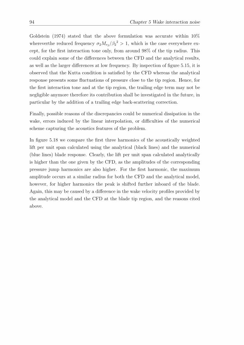
94 Chapter 5 Wake interaction noise
Goldstein (1974) stated that the above formulation was accurate within 10%
whereverthe reduced frequency σ2Mr2/β22 > 1, which is the case everywhere ex-
cept, for the first interaction tone only, from around 98% of the tip radius. This
could explain some of the differences between the CFD and the analytical results,
as well as the larger differences at low frequency. By inspection of figure 5.15, it is
observed that the Kutta condition is satisfied by the CFD whereas the analytical
response presents some fluctuations of pressure close to the tip region. Hence, for
the first interaction tone and at the tip region, the trailing edge term may not be
negligible anymore therefore its contribution shall be investigated in the future, in
particular by the addition of a trailing edge back-scattering correction.
Finally, possible reasons of the discrepancies could be numerical dissipation in the
wake, errors induced by the linear interpolation, or difficulties of the numerical
scheme capturing the acoustics features of the problem.
In figure 5.18 we compare the first three harmonics of the acoustically weighted
lift per unit span calculated using the analytical (black lines) and the numerical
(blue lines) blade response. Clearly, the lift per unit span calculated analytically
is higher than the one given by the CFD, as the amplitudes of the corresponding
pressure jump harmonics are also higher. For the first harmonic, the maximum
amplitude occurs at a similar radius for both the CFD and the analytical model,
however, for higher harmonics the peak is shifted further inboard of the blade.
Again, this may be caused by a difference in the wake velocity profiles provided by
the analytical model and the CFD at the blade tip region, and the reasons cited
above.

Chapter 5 Wake interaction noise 95
(a)
(b)
0.02
0.01
8 a.. -
0
-.. a.
<'.I -
ro Q)
Cl:'.
-0.01
0.5 1.5 2 -0.02
Figure 5.15: Airfoil response for k = 1. (a) predicted levels, (b) numericalresults.

96 Chapter 5 Wake interaction noise
(a)
0.02
0.01
8 a.. -
0
-.. a.
<'.I -
ro Q)
Cl:'.
-0.01
0.5 1.5 2 -0.02
(b)
0.02
0.01
0 s ro
-0.01
11
Rh
2 0.5 1 1.5 2 -0.02
x2
Figure 5.16: Airfoil response for k = 2. (a) predicted levels, (b) numericalresults.

Chapter 5 Wake interaction noise 97
(a)
(b)
Figure 5.17: Airfoil response for k = 3. (a) predicted levels, (b) numericalresults.
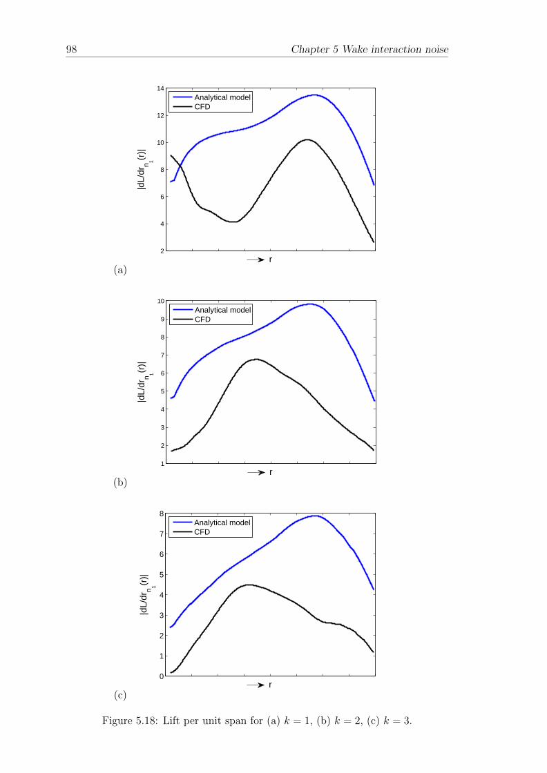
98 Chapter 5 Wake interaction noise
(a)
2
4
6
8
10
12
14
r
|dL/
drn 1(r
)|
Analytical modelCFD
(b)
1
2
3
4
5
6
7
8
9
10
r
|dL/
drn 1(r
)|
Analytical modelCFD
(c)
0
1
2
3
4
5
6
7
8
r
|dL/
drn 1(r
)|
Analytical modelCFD
Figure 5.18: Lift per unit span for (a) k = 1, (b) k = 2, (c) k = 3.

Chapter 5 Wake interaction noise 99
5.3 Wake interaction noise prediction
The interaction noise due to the impingement of the front rotor viscous wakes
onto the rear rotor blades can be calculated using the radiation formula given by
equation (4.30) from section 4 giving
PL(x, t) =+∞∑
k=−∞
+∞∑m=−∞
rt2∫rh2
iB2
4πSexp
i(n2Ω2 + n1Ω1)
(t− re
c0
)
× exp−i(n2B2 − n1B1)
(φ′ +
π
2
)exp −iΦs − ikY ll
× kY lJn1B1−b2B2
(ωrySsc0
)ΨL dry, (5.23)
where ΨL =dL
dris the acoustically-weighted unsteady lift per unit span.
Noise predictions made using the method described in the previous sections are
compared with noise measurements made during testing of Airbus’s Z08 rig with
Rolls-Royce’s blades during the Z08 test campaign conducted in the DNW large,
low speed wind tunnel (see Chapter 2), as well as with noise predictions made
using the blade response given by the CFD. Figure 5.19 shows the noise spectrum
at θ′ = 90 for a particular experiment conducted with an isolated rig running
at a condition representative of take-off at zero angle of attack. All the results
presented in the present section are representative of this particular operating
condition.
Each tone emanates from an integration of ‘sources’ over the radial coordinate ry.
Parry (1988) introduced that the radiation efficiency of the interaction tones is
dependent on the non-dimensional sonic radius z∗, the radius at which the source
would be moving toward the observer at sonic velocity, defined by
z∗ =ν(1−Mx cos θ′)c0
(n1B1Ω1 + n2B2Ω2)Rt2 sin θ′. (5.24)
A detailed discussion about the sonic radius given by Kingan et al. (2014) suggests
that if the sonic radius lies inboard of the tip (0 < |z∗| < 1), the tones will radiate
efficiently in the vicinity of z∗. In the present case, the absolute value of the sonic
radius related to the frequency for each interaction tone is plotted in figure 5.20.
Note that tones that do not appear in the spectrum are labelled using red font,
whereas tones which do appear are labelled in black. It is clearly observed that
tones for which the sonic radius lies somewhat outboard of the tip (i.e. tones for
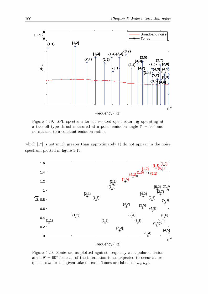
100 Chapter 5 Wake interaction noise
104
Frequency (Hz)
SP
L
Broadband noiseTones
4,4
2,1
1,3
2,2
3,1
3,3
1,1
2,5
2,4
1,42,33,2
1,2
4,2
3,5
2,72,8
4,52,6
4,33,63,4
5,2 5,3
10 dB
Figure 5.19: SPL spectrum for an isolated open rotor rig operating ata take-off type thrust measured at a polar emission angle θ′ = 90 andnormalized to a constant emission radius.
which |z∗| is not much greater than approximately 1) do not appear in the noise
spectrum plotted in figure 5.19.
104
0
0.2
0.4
0.6
0.8
1
1.2
1.4
1.6
Frequency (Hz)
|z* |
1,1
1,2
1,3
1,4
1,5
1,71,8 1,9
2,1
2,2
2,3
2,4
2,5
2,6
2,7
2,83,1
3,2
3,3
3,4
3,5
3,6
4,1
4,2
4,3
4,4
4,5
5,2
5,3
6,1
5,11.6
Figure 5.20: Sonic radius plotted against frequency at a polar emissionangle θ′ = 90 for each of the interaction tones expected to occur at fre-quencies ω for the given take-off case. Tones are labelled n1, n2.

Chapter 5 Wake interaction noise 101
The predicted polar directivities of a selection of interaction tones are compared
with the wind tunnel measurements and the CFD-based calculations in figures 5.21
to 5.26. It is important to note that, once the wake profiles have been obtained
(on this occasion, via unsteady CFD) the additional wake decay, unsteady blade
response and acoustic radiation can be performed immediately, and very quickly,
using the analytical formulae (5.23). The predictions show good agreement with
the experimental data for both the low frequency and the high frequency tones
in terms of absolute level and in terms of the envelope shape of the directivity
characteristics, except at some particular observer locations (note that some of the
discrepancies could be due to measurements uncertainties). There is also a good
agreement between the CFD-based calculations and the analytical model in terms
of overall trend. In terms of noise levels, the numerical and analytical results agree
within 1dB to 10dB margin at a wide range of angles and frequencies. However,
larger differences are observed at distinct locations and, at few frequencies, over
a wide range of angles, e.g. between 100 and 150 for the tone 3, 4, see figure
5.24. Some phase shifts are also observed between the directivity lobes of the tones
predicted by each method.
Note here that the unsteady velocities produced by the rotors’ bound potential
fields, and by the front rotor tip vortex (which are not included in these results)
affect both the total unsteady flow field and the levels of the radiated interac-
tion tones at some frequencies and some observer positions; particularly as their
directivity characteristics differ from those of convected wake interaction tones.
However, it is most likely that the low frequency results will be affected as the
potential fields decay rapidly with frequency, and because the tip vortex contri-
bution is likely to be small for the cropped rear row used in our example. Indeed,
the results in section 5.2.3 above, showed that the harmonics of the velocity up-
wash onto the rear rotor are affected by the potential field component of the flow,
particularly at the lower harmonics. The potential field effects are investigated
further in section 6.
Other possible sources of discrepancies between the analytical and the numerical
results could be attributed to numerical errors (e.g. the discontinuity at the sliding
plane or numerical dissipation), or the assumptions of the method, for example
the neglect of the wake skew or sweep effects in the analytical blade response
(which would affect both the phase and levels). Since the differences is noise levels
are directly linked to the differences in the lift distributions, future efforts will be
concentrated on the improvement of the modelling of the source and the blade
response.

102 Chapter 5 Wake interaction noise
20 40 60 80 100 120 140 160Polar emission angle (°)
SP
L
Analytical modelMeasurementsCFD
10 dB
Figure 5.21: Polar directivity of the tone 1, 1 for a given take-off casecompared with wind tunnel measurements and CFD data.
20 40 60 80 100 120 140 160Polar emission angle (°)
SP
L
Analytical modelMeasurementsCFD
10 dB
Figure 5.22: Polar directivity of the tone 1, 2 for a given take-off casecompared with wind tunnel measurements and CFD data.

Chapter 5 Wake interaction noise 103
20 40 60 80 100 120 140 160Polar emission angle (°)
SP
L
Analytical modelMeasurementsCFD
10 dB
Figure 5.23: Polar directivity of the tone 2, 2 for a given take-off casecompared with wind tunnel measurements and CFD data.
20 40 60 80 100 120 140 160Polar emission angle (°)
SP
L
Analytical modelMeasurementsCFD
10 dB
Figure 5.24: Polar directivity of the tone 3, 4 for a given take-off casecompared with wind tunnel measurements and CFD data.

104 Chapter 5 Wake interaction noise
20 40 60 80 100 120 140 160Polar emission angle (°)
SP
L
Analytical modelMeasurementsCFD
10 dB
Figure 5.25: Polar directivity of the tone 3, 6 for a given take-off casecompared with wind tunnel measurements and CFD data.
20 40 60 80 100 120 140 160Polar emission angle (°)
SP
L
Analytical modelMeasurementsCFD
10 dB
Figure 5.26: Polar directivity of the tone 4, 4 for a given take-off casecompared with wind tunnel measurements and CFD data.

Chapter 5 Wake interaction noise 105
5.4 Concluding remarks
A hybrid method which can be used to predict the development of the front rotor
viscous wakes and to calculate the far-field tonal noise caused by the impingement
of such wakes on the advanced open rotor’s downstream blades has been developed.
The method uses a simple two-dimensional analytical model for which the wake
start-up characteristics are taken from data on a CFD plane between the two blade
rows, and convected to the leading edge of the downstream rotor. Comparisons
at other wake propagation distances show that the method gives good agreement
with the CFD for most radii. However, possible inaccuracies in the numerical
scheme or some phenomena such as the bound potential fields of both blade rows,
the tip vortex of the front rotor, and stream tube contraction are not included and
account for some of the discrepancies in the total noise predictions.
The analytical method for predicting the unsteady flow field associated with the
upstream rotor wakes and the radiated far-field tonal noise was assessed by compar-
ison with wind tunnel measurements and CFD data. Comparisons of the unsteady
loading on the downstream blade calculated using both the CFD simulation and
the hybrid method showed promising results in the ability to predict the general
behaviour of the flow field around the blades. The noise predictions show satisfac-
tory agreement between the wind tunnel measurements, the analytical model, and
the CFD-based method in a wide range of observer locations and frequencies. Yet,
the origins of the discrepancies observed in the analysis need further investigation,
in particular the the source and blade response modelling, as well as the reasons
cited above.


Chapter 6
Potential field interactions
6.1 Introduction
Along with the viscous wakes, the bound potential field of each rotor blade pro-
duces an ’incident’ unsteady (periodic) flow field on the blades of the adjacent
rotor. The potential field is produced by the blade thickness and loading (due
to the airfoil’s camber and angle of attack). For a single rotor blade, the bound
potential field decays away from the rotor relatively quickly whereas the viscous
wake convects with the local flow. Because the blade rows can be separated by
a sufficient distance to ensure that the potential field interactions are much less
significant than the viscous wake source, the potential field effects have, to the
author’s knowledge, received little attention in the literature. For smaller distance
between the two blade rows, the potential field effects can become significant.
Kingan et al. (2014) showed that for some cases the interaction between the po-
tential field of a blade row with the adjacent rotor can be a dominant source of
tonal noise.
Kemp and Sears (1953) first derived an expression for the potential field produced
by a cascade of blades. They only accounted for the loading component, modelling
each blade as a point vortex of strength equal to the steady blade circulation.
Parry (1988) extended the analysis to incorporate the compressibility effects and
derived an expression for the potential field due to blade thickness. In the latter the
blades were modelled as a cascade of point sources whose strength was determined
from the potential field of an ellipse. In the present section, the loading and
thickness components of the potential field produced by each blade are modeled
by a distribution of sources along the blade chordline. The upwash on the adjacent
107

108 Chapter 6 Potential field interactions
blade and the corresponding blade response are then formulated. The effect of
varying the airfoil geometry is also investigated. In section 6.4 the potential field
interaction noise is calculated for a given take-off case. Results are compared with
Parry’s model for point sources, and with wind tunnel measurements and URANS
CFD data. For convenience, the theory presented in this chapter will be termed
’model 1’ and Parry’s formulation will be termed ’model 2’. The latter is presented
in Appendix D.
The velocity produced by the bound potential field of a rotor blade is equal to the
gradient of the velocity potential φ
u = 5φ. (6.1)
The velocity field u is irrotational and the potential satisfies the inhomonegeous
Laplace equation
52 φ = S, (6.2)
where S represents a source term. Since the governing equations are linear, solu-
tions may be superimposed linearly. The solution is thus written as the sum of
the free-stream potential and a disturbance potential. The latter is decomposed
into two terms, one giving the field due to thickness, and the other the potential
due to loading, see Ashley and Landahl (1965). Thus, the thickness and loading
problems will be solved separately. For each problem, the potential field produced
by the compressible flow over a thin airfoil may be regarded as the potential field
produced by a distribution of elementary sources of strength f along the blade
chord line.
φ(X, Y ) =
∫ c2
−c2
f(Xs)ϑ((X, Y )|(Xs, 0)) dXs, (6.3)
where c is the blade chordlength and ϑ((X, Y )|(Xs, 0)) is the potential produced
by one elementary source of unit strength, located at X = Xs and Y = 0, and
satisfying the governing equations. The value of f is to be determined for the
thickness problem and the loading problem independently. The blade geometry
and the coordinates X, Y are shown in figure 6.1.
The location of the upper (+) and lower (−) surface of the airfoil is

Chapter 6 Potential field interactions 109
X
Y
c/2
Y +(X)
Y −(X)
U∞
Camber line
Chord line
−c/2
Figure 6.1: Airfoil geometry.
Y ± = ±tmax2G(X) + θh(X)− γX, (6.4)
where the functions G(X) and h(X) represent dimensionless thickness and camber
distributions along the blade chord respectively, tmax is the maximum thickness,
γ is the angle of attack, and θ represents the maximum camber. The free-stream
potential is related to the free-stream velocity Ur by
φ∞ = Urx. (6.5)
6.2 Upstream interactions
In this section we derive expressions for the unsteady potential field induced by
the downstream blade row, the upwash incident on the upstream airfoil and the
airfoil’s response. The blade rows are modeled by infinite cascades of equally
spaced flat airfoils. We note s =2πr
Bis the distance between two airfoils. The
configuration is shown in figure 6.2, where g is the gap between the two rotors,
α is the blade stagger angle, X, Y are the coordinates parallel and normal to
the chordline, and the x, y coordinate system is related to the cylindrical polar
coordinate system x, r, ϕ, via y = rϕ. The subscripts 1 and 2 denote values
associated with the upstream and downstream rotor respectively.
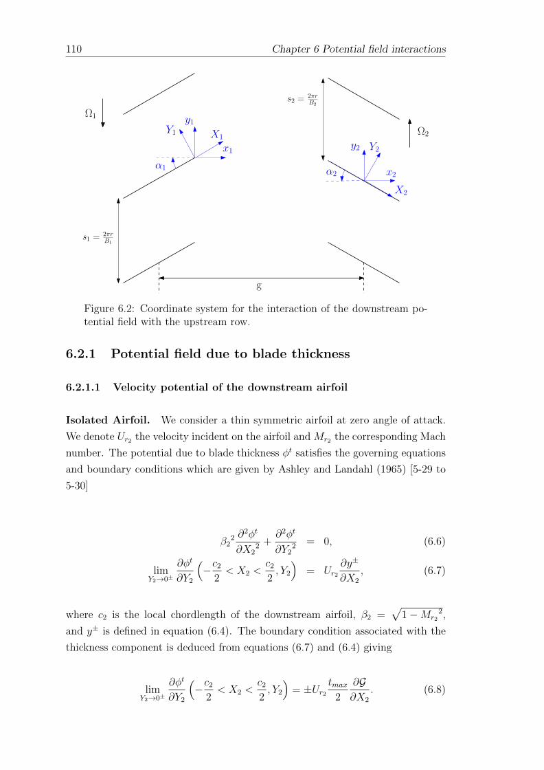
110 Chapter 6 Potential field interactions
X1Y1
x1
x2
Y2
X2
α1 α2
y1
y2
Ω1
Ω2
g
s2 =2πrB2
s1 =2πrB1
Figure 6.2: Coordinate system for the interaction of the downstream po-tential field with the upstream row.
6.2.1 Potential field due to blade thickness
6.2.1.1 Velocity potential of the downstream airfoil
Isolated Airfoil. We consider a thin symmetric airfoil at zero angle of attack.
We denote Ur2 the velocity incident on the airfoil and Mr2 the corresponding Mach
number. The potential due to blade thickness φt satisfies the governing equations
and boundary conditions which are given by Ashley and Landahl (1965) [5-29 to
5-30]
β22 ∂
2φt
∂X22 +
∂2φt
∂Y22 = 0, (6.6)
limY2→0±
∂φt
∂Y2
(−c2
2< X2 <
c2
2, Y2
)= Ur2
∂y±
∂X2
, (6.7)
where c2 is the local chordlength of the downstream airfoil, β2 =√
1−Mr22,
and y± is defined in equation (6.4). The boundary condition associated with the
thickness component is deduced from equations (6.7) and (6.4) giving
limY2→0±
∂φt
∂Y2
(−c2
2< X2 <
c2
2, Y2
)= ±Ur2
tmax2
∂G∂X2
. (6.8)

Chapter 6 Potential field interactions 111
Introducing the stretched Prandtl-Glauert coordinates χ2, ζ2 = X2/β2, Y2, and
substituting χ2 into equation (6.6) yields a two dimensional form of the Laplace
equation. The potential ϑt of a point source located at χ2 = Xs/β2 and ζ2 = 0
actually satisfies
∂2ϑt
∂χ22
+∂2ϑt
∂ζ22 = δ
(χ2 −
Xs
β2
)δ(ζ2). (6.9)
The above equation can be written in the X2, Y2 coordinate system as
β22 ∂
2ϑt
∂X22 +
∂2ϑt
∂Y22 = β2δ (X2 −Xs) δ(Y2). (6.10)
An elementary singular solution to equation (6.10) is
ϑt((X2, Y2)|(Xs, 0)) =1
2πlog
(1
β2
√(X2 −Xs)2 + β2
2Y22
). (6.11)
The airfoil thickness effect is modeled as a distribution of two dimensional ele-
mentary sources and sinks of volume flow rate per unit area f t (m.s−1) located at
points Xs = Xs, Ys = 0 along the blade chordline, see figure 6.3. The poten-
tial can be obtained by integrating the contribution of each point source over the
airfoil chord as follows
φt(X2, Y2) =1
2π
− c22∫
−c22
f t(Xs2) log
(1
β2
√(X2 −Xs)2 + β2
2Y22
)dXs. (6.12)
Hence
∂φt
∂Y2
=1
2π
c22∫
−c22
f t(Xs)β2
2Y
(X2 −Xs)2 + β22Y2
2 dXs. (6.13)
Taking the limit of equation (6.13) as Y2 → 0±, noting that
limY2→0±
β22Y2
(X2 −Xs)2 + β22Y2
2 = ±β2πδ(X2 −Xs), (6.14)

112 Chapter 6 Potential field interactions
and equating the above result with the boundary condition defined in equation
6.7 gives the following expression for the source strength.
f t(X2) =Ur2tmaxβ2
∂G(X2)
∂X2
. (6.15)
c2/2
x2
y2
G(X2)
Ur2
Xs
−c2/2
Y2
X2
α2
Figure 6.3: Thickness source distribution.
To allow fast and simple calculations of the velocity potential, we chose to model
the airfoil’s thickness distribution using two sine functions whose coefficients are
deduced from a given airfoil’s geometry. The non-dimensional thickness function
G(X2) is thus expressed as
G(X2) = sin
(π
2Xm
(X2 +
c2
2
))if − c2
2< X2 < −
c2
2+Xm,
G(X2) = sin
(π
2+π
2
X2 + c22−Xm
c2 −Xm
)if − c2
2+Xm < X2 <
c2
2.
(6.16)
From Equations (6.15) and (6.16), the source strength is
f t(X2) =
Ur2tmaxπ
2β2Xm
cos
(π
2Xm
(X2 +
c2
2
))if − c2
2< X2 < −
c2
2+Xm,
f t(X2) = − Ur2tmaxπ
2β2(c2 −Xm)sin
(π
2
X2 + c22−Xm
c2 −Xm
). if − c2
2+Xm < X2 <
c2
2.
(6.17)
Hence the potential due to blade thickness of a single airfoil is given by

Chapter 6 Potential field interactions 113
φt =Ur2tmax
4β2
1
Xm
−c22
+Xm∫−c2
2
cos
(π
2Xm
(X2 +
c2
2
))log
(1
β2
√(X2 −Xs)2 + β2
2Y22
)dXs
− 1
c2 −Xm
c22∫
−c22
+Xm
sin
(π
2
X2 + c22−Xm
c2 −Xm
)log
(1
β2
√(X2 −Xs)2 + β2
2Y22
)dXs
.(6.18)
The velocity potential around an isolated airfoil in incompressible flow (β2 = 1) is
illustrated in figures 6.4 calculated using equation (6.18). In figure 6.5 the influence
of the downstream airfoil’s geometry on the upwash incident on the upstream airfoil
is investigated at r = 60%Rt1 at various axial locations. The upwash velocity
calculated using the thickness distribution defined in equation (6.16) (geometry
A) is compared to that calculated using the thickness distribution function for an
elliptic airfoil (geometry B)
Gellipse(X2) =
√1−
(2X2
c2
)2
. (6.19)
Figure 6.4: Velocity potential calculated with model 1.
It is important to note that there is a good agreement between model 1 and model 2
when using the same geometry. There is a notable difference in values between the

114 Chapter 6 Potential field interactions
upwash velocities calculated using geometries A and B as input in the distributed
model at a wide range of axial locations. This shows that the type of profile
inputed in the model greatly influences the results. The differences between the
two models are assessed further in figure 6.6 in terms of percentage difference in the
amplitude of the upwash velocity incident on the upstream airfoil at a fixed radius
and various azimuthal locations. Close to the downstream airfoil’s leading edge,
differences up to 60% are notable. Further away from the airfoil the differences
decrease but remain around 35%. When using the geometry of an ellipse in the
distributed model, which was the geometry used in Parry’s model, the differences
in upwash velocity amplitude are much lower close to the downstream airfoil (up
to ≈ 30% one chordlength away and up to ≈ 10% two chordlength away) and the
two models converge in the far field within an error of about 5 %, see figure 6.7.
−20 −15 −10 −5 010
−6
10−5
10−4
10−3
10−2
x2 / c
2
Nor
mal
ized
upw
ash
velo
city
Model 1 − Geometry AModel 2 − Geometry BModel 1 − Geometry B
Figure 6.5: Upwash velocity (normalized against the free stream velocity)calculated using models 1 and 2 at r = 60%Rt1 . Geometry A: sum of sinefunctions; Geometry B: ellipse.
Indeed, in Appendix D it is shown that Parry’s expression for a very thin ellipse
(tmax << c2) (D.7) can be recovered from the formulation of the distributed source
model and the error between the two models can be determined analytically. Tak-
ing into account the distribution of sources along the airfoil chordline can thus have
a non negligible influence on the resulting potential field when the gap between
the two rotors is less than two chordlengths.

Chapter 6 Potential field interactions 115
−20 −15 −10 −5 030
35
40
45
50
55
60
65
x2 / c
2
% d
iffer
ence
in u
pwas
h ve
loci
ty
y2 = 0
y2 = 3 c
2
y2 = 6 c
2
Figure 6.6: Percentage difference in upwash velocity between model 1 (withgeometry A) and model 2.
−20 −15 −10 −5 0−10
−5
0
5
10
15
20
25
30
35
x2 / c
2
% d
iffer
ence
in u
pwas
h ve
loci
ty
y2 = 0
y2 = 3 c
2
y2 = 6 c
2
Figure 6.7: Percentage difference in upwash velocity between model 1 (us-ing an elliptic geometry) and model 2.
116 Chapter 6 Potential field interactions
Cascade of airfoils. Consider now the potential produced by a cascade of
equally spaced airfoils of the downstream row at locations y2 = n2s2, as described
by figure 6.2. The x2, y2 and X2, Y2 coordinate systems are related by
X2 = cosα2 x2 − sinα2 y2,
Y2 = sinα2 x2 + cosα2 y2,(6.20)
and x2 = cosα2X2 + sinα2 Y2,
y2 = − sinα2X2 + cosα2 Y2,(6.21)
The governing equation (6.10) becomes
∂2ϑt
∂χ22
+∂2ϑt
∂ζ22 = β2
+∞∑n2=−∞
δ (X2 −Xs + n2s2 sinα2) δ(Y2 − n2s2 cosα2). (6.22)
The above equation can be written in terms of x2, y2 coordinates making use of
the following theorem (see Izzo (2005))
δ [x− x(y)] =∑i
δ [y − yi]
|J |y=yi
, (6.23)
where J =∂xi∂yi
is the Jacobian of the transformation x(yi) and yi are the solutions
to the equation x = x(yi) . In the present case the Jacobian determinant related
to the change from the X2, Y2 to the x2, y2 coordinates is
det
[∂x2, y2∂X2, Y2
]= 1. (6.24)
Note that the arguments of the Dirac delta functions in equation (6.22) are related
to the x2, y2 coordinates by
X2 −Xs + n2s2 sinα2 = (x2 −Xs cosα2) cosα2 − (y2 − n2s2 +Xs sinα2) sinα2,
Y2 − n2s2 cosα2 = (x2 −Xs cosα2) sinα2 + (y2 − n2s2 +Xs sinα2) cosα2,
(6.25)

Chapter 6 Potential field interactions 117
and that they equal zero if and only if x2 = Xs2 cosα2 and y2 = n2s2 −Xs sinα2.
Therefore
δ (X2 −Xs + n2s2 sinα2) δ(Y2−n2s2 cosα2) = δ (x2 −Xs cosα2) δ(y2−n2s2+Xs sinα2).
(6.26)
Equation (6.22) can be rewritten by making use of equation (6.26) giving
5c2ϑt = β2
+∞∑n2=−∞
δ (x2 −Xs cosα2) δ(y2 +Xs sinα2 − n2s2), (6.27)
with
5c2 =
(sin2 α2 + β2
2 cos2 α2
) ∂2
∂x22
+ 2 sinα2 cosα2
(1− β2
2) ∂2
∂x2∂y2
+(cos2 α2 + β2
2 sin2 α2
) ∂2
∂y22. (6.28)
Applying Poisson’s summation formula to equation (6.27) leads to
5c2ϑt =
β2
s2
δ (x2 −Xs cosα2)+∞∑
n2=−∞exp
−2iπ
n2
s2
(y2 +Xs sinα2)
. (6.29)
To calculate the velocity potential ϑt, it is convenient to use the Fourier tranform
pair
ϑt(kx, ky) =1
(2π)2
∫∫ +∞
−∞ϑt(x2, y2) exp ikxx2 + ikyy2 dx2 dy2, (6.30)
ϑt(x2, y2) =
∫∫ +∞
−∞ϑt(kx, ky) exp −ikxx2 − ikyy2 dkx dky. (6.31)
Hence, performing the Fourier transform of equation (6.29) yields

118 Chapter 6 Potential field interactions
Y2
X2
s2 =2πrB2
y2
x2α2
Ur2
Figure 6.8: Thickness source cascade distribution.
ϑt(kx, ky) = − β2
2πs2
+∞∑n2=−∞
δ(ky −Ky)
Dexp −iKy2Xs sinα2 + ikxXs cosα2 ,
(6.32)
where Ky2 =2πn2
s2
and
D = kx2(sin2 α2 + β2
2 cos2 α2
)+ 2 sinα2 cosα2
(1− β2
2)kxKy2
+ Ky2
2(cos2 α2 + β2
2 sin2 α2
), (6.33)
This yields
ϑt(x2, y2) = − β2
2πs2
+∞∑n2=−∞
exp −iKy2(y2 +Xs sinα2)∫ +∞
−∞
exp −ikx(x2 −Xs cosα2)D
dkx.
(6.34)
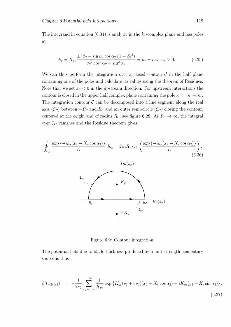
Chapter 6 Potential field interactions 119
The integrand in equation (6.34) is analytic in the kx-complex plane and has poles
at
kx = Ky2
±i β2 − sinα2 cosα2
(1− β2
2)
β22 cos2 α2 + sin2 α2
= κr ± i κc, κc > 0. (6.35)
We can thus perform the integration over a closed contour C in the half plane
containing one of the poles and calculate its values using the theorem of Residues.
Note that we set x2 < 0 in the upstream direction. For upstream interactions the
contour is closed in the upper half complex plane containing the pole κ+ = κr+iκc.
The integration contour C can be decomposed into a line segment along the real
axis (CR) between −RC and RC and an outer semi-circle (CC) closing the contour,
centered at the origin and of radius RC, see figure 6.28. As RC →∞, the integral
over CC vanishes and the Residue theorem gives
∮CR
exp −ikx(x2 −Xs cosα2)D
dkx = 2πiResκ+
(exp −ikx(x2 −Xs cosα2)
D
).
(6.36)
−Ky
Ky
Re(kx)
Im(kx)
Cc
Cr−RC RC
Figure 6.9: Contour integration.
The potential field due to blade thickness produced by a unit strength elementary
source is thus
ϑt(x2, y2) = − 1
2s2
+∞∑n2=−∞
1
Ky2
exp Ky2(ν1 + i ν2)(x2 −Xs cosα2)− iKy2(y2 +Xs sinα2) .
(6.37)

120 Chapter 6 Potential field interactions
where
ν1 =β2
β22 cos2 α2 + sin2 α2
, (6.38)
ν2 =sinα2 cosα2
(1− β2
2)
β22 cos2 α2 + sin2 α2
. (6.39)
In order to calculate the velocity potential due to blade thickness for a distributed
source, we must determine the source strength f t, i.e. the thickness distribution
function G must be defined, and evaluate
φt(x2, y2) = −Ur2tmax2s2β2
+∞∑n2=−∞
1
Ky2
exp Ky2(ν1 + i ν2)x2 − iKy2y2
×
c22∫
−c22
exp −Ky2(ν1 + i ν2)Xs cosα2 − iKy2Xs sinα2∂G∂X2
∣∣∣X2=Xs
dXs.
(6.40)
The velocity potential is obtained by inserting equation (6.16) into equation (6.40),
i.e.
φt = −Ur2tmaxπ4s2β2
+∞∑n=−∞
1
Ky2
exp Ky2(ν1 + i ν2)x2 − iKy2y2 [I1 + I2] , (6.41)
where
I1 =1
Xm
−c22
+Xm∫−c2
2
cos
(π
2Xm
(Xs +
c2
2
))exp −Ky2 [(ν1 + i ν2) cosα2 + i sinα2]Xs dXs,
I2 =−1
c2 −Xm
c22∫
−c22
+Xm
sin
(π
2
Xs + c22−Xm
c2 −Xm
)exp −Ky2 [(ν1 + i ν2) cosα2 + i sinα2]Xs dXs.
(6.42)

Chapter 6 Potential field interactions 121
The integrals I1 and I2 can be easily calculated giving
I1 =2 exp
E2
(c22−Xm
)[π + 2E2Xm exp E2Xm]
π2 + 4E22X2
m
, (6.43)
I2 = −2[π exp
E2
(c22
+Xm
)− 2 exp
− c2
2E2
(c2 −Xm)E2
]π2 + 4E2
2(c2 −Xm)2, (6.44)
where
E2 = Ky2 [(ν1 + i ν2) cosα2 + i sinα2] . (6.45)
According to equation (D.8) in Appendix D, in the cascade representation the
velocity potentials given by model 1 and model 2 are proportional by a factor
F =(I1 + I2)(β2
2 cos2 α2 + sin2 α2)
β2Ky2(β2 a+ b)(β2 cosα2 + i sinα2), (6.46)
with a = tmax/2 and b = c2/2.
Note that the velocity potential around an ellipse can be determined inserting
equations (6.19) into equation (6.40) to give
φtellipse = −Ur2tmax2s2β2
+∞∑n=−∞
1
Ky2
exp Ky(ν1 + i ν2)x2 − iKy2y2 Ie, (6.47)
where
Ie = πI1
(c2
2Ky2 [(ν1 + i ν2) cosα2 + i sinα2]
), (6.48)
and I1 is the modified Bessel function of the first kind with order 1.
6.2.1.2 Upwash on the upstream airfoil
Consider an isolated airfoil of the upstream row in the coordinate system defined
in figure 6.2. Recall that the suffixes 1 and 2 denote values associated with the

122 Chapter 6 Potential field interactions
upstream and downstream rotor respectively and that x2 < 0 in the upstream
direction. The upwash normal to the airfoil is given by
u1 = − sinα1∂φt
∂x2
+ cosα1∂φt
∂y2
, (6.49)
where α1 is the stagger angle of the upstream airfoil. Applying equation (6.49) to
equation (6.47), the upwash on the upstream airfoil is given by
u1 =Ur2tmaxπ
4s2β2
[(ν1 + iν2) sinα1 + i cosα1]+∞∑
n=−∞exp Ky(ν1 + i ν2)x2 − iKy2y2 [I1 + I2] .
(6.50)
The (x1, y1) and (x2, y2) coordinate systems defined in figure 6.2 are related by
x2 = x1 −(g − c1
2cosα1
),
y2 = y1 +c1
2sinα1 − r(Ω1 + Ω2)t, (6.51)
where g is the gap between the midchords of the upstream and downstream rotors
and c1 is the local chordlength of the upstream airfoil. The (x1, y1) and (X1, Y1)
coordinate systems are related by
x1 = X1 cosα1 − Y1 sinα1,
y1 = X1 sinα1 + Y1 cosα1. (6.52)
Inserting equations (6.51) and (6.52) into equation (6.50), one harmonic of the
upwash normal to the upstream airfoil can be written in the form
u1 = W t1 exp λx2X1 + λy2Y1 + iω2t , (6.53)
where

Chapter 6 Potential field interactions 123
W t1 = − λy2
Ur2tmax8n2β2
exp A1 [I1 + I2] ,
A1 = −Ky2
(η2
(g − c1
2cosα1
)+ i
c1
2sinα1
),
η2 = ν1 + iν2,
λx2 =Ky2(η2 cosα1 − i sinα1),
λy2 = −Ky2(η2 sinα1 + i cosα1),
ω2 =Ky2r(Ω1 + Ω2).
(6.54)
Note that the harmonic number n2 is assumed to be positive here. Figure 6.10
shows the ten first harmonics of the upwash at r ≈ 60%Rt1 at the upstream
rotor’s trailing edge calculated using both model 1 and model 2. Since model
2 utilizes the geometry of an ellipse, model 1 is assessed for both the geometry
defined by the thickness distribution from equation (6.16) (labelled geometry A)
and the geometry of an ellipse (labelled geometry B). When using the latter, there
is a good agreement between the two models at low harmonic counts. However
at higher frequencies the consideration of a distributed profile creates significant
differences in the harmonic content in comparison to the one from Parry’s source
representation. Note that there is a good qualitative agreement between the results
calculated using geometries A and B as inputs to model 1.
1 2 3 4 5 6 7 8 9 1010
−25
10−20
10−15
10−10
10−5
100
n2
|Wt 1| /
U∞
Model 1 − Geometry AModel 1 − Geometry BModel 2 − Geometry B
Figure 6.10: Magnitude of the first ten harmonics of the upwash velocitynormalized by the free stream velocity at the upstream blade’s trailingedge at r ≈ 60%Rt1 . Geometry A: sum of sine functions; Geometry B:ellipse.

124 Chapter 6 Potential field interactions
The effect of varying the airfoil’s geometry is assessed further in figures 6.11 and
6.12 in which the normalized amplitude of, respectively, the first and fifth upwash
harmonic is calculated at all spanwise locations along the upstream airfoil’s trailing
edge. In figure 6.11 both models provide amplitudes of similar order of magnitude,
although model 1 dispenses a difference in the peak amplitude by approximately
12% due to the change of the airfoil’s geometry. Figure 6.12 shows, for the same
geometry, a significant difference between the amplitudes calculated using model 1
and model 2 along most of the blade span. This suggests that at high frequencies
the airfoil can no longer be assimilated as a point source and that the variation
of the airfoil’s thickness along its chordline needs to be accounted for. The figure
also exhibits a greater dependance on the geometry at high frequency. One should
bear in mind, though, that the geometry A does not have a blunt leading edge
and thus does not constitute a realistic representation of the airfoil. Consequently
the thickness effects at the leading edge are likely to differ from the reality on the
prediction of the potential field.
0
1
2
3
4
5
6x 10
−4
r
|W1t | /
U∞
Model 1 − Geometry AModel 1 − Geometry BModel 2 − Geometry B
Figure 6.11: Amplitude of the first upwash harmonic (normalized againstthe free stream velocity U∞) at the upstream blade’s trailing edge. Geom-etry A:sum of sine functions; Geometry B: ellipse.
Consider now a third geometry for which the airfoil has a blunt leading edge
and a sharp trailing edge. The geometry, labelled geometry C, is defined as a
combination of geometries A and B as follows.

Chapter 6 Potential field interactions 125
0
0.5
1
1.5
2
2.5
3
3.5x 10
−11
r
|W1t | /
U∞
Model 1 − Geometry AModel 1 − Geometry BModel 2 − Geometry B
Figure 6.12: Amplitude of the fifth upwash harmonic (normalized againstthe free stream velocity U∞) at the upstream blade’s trailing edge. Geom-etry A: sum of sine functions; Geometry B: ellipse.
G(X2) =
√1−
(X2 + c2/2−Xm
Xm
)2
if − c2
2< X2 < −
c2
2+Xm,
G(X2) = sin
(π
2+π
2
X2 + c22−Xm
c2 −Xm
)if − c2
2+Xm < X2 <
c2
2.
(6.55)
The velocity potential of the downstream airfoil becomes
φt = −Ur2tmax2s2β2
+∞∑n=−∞
1
Ky2
exp Ky2(ν1 + i ν2)x2 − iKy2y2 [I1,C + I2,C ] , (6.56)
where
I1,C = πI1(XmE2) exp −E2(Xm − c2/2) , (6.57)
I2,C =π
2I2. (6.58)
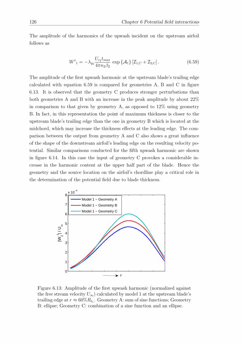
126 Chapter 6 Potential field interactions
The amplitude of the harmonics of the upwash incident on the upstream airfoil
follows as
W t1 = −λy2
Ur2tmax4πn2β2
exp A1 [I1,C + I2,C ] . (6.59)
The amplitude of the first upwash harmonic at the upstream blade’s trailing edge
calculated with equation 6.59 is compared for geometries A, B and C in figure
6.13. It is observed that the geometry C produces stronger perturbations than
both geometries A and B with an increase in the peak amplitude by about 22%
in comparison to that given by geometry A, as opposed to 12% using geometry
B. In fact, in this representation the point of maximum thickness is closer to the
upstream blade’s trailing edge than the one in geometry B which is located at the
midchord, which may increase the thickness effects at the leading edge. The com-
parison between the output from geometry A and C also shows a great influence
of the shape of the downstream airfoil’s leading edge on the resulting velocity po-
tential. Similar comparisons conducted for the fifth upwash harmonic are shown
in figure 6.14. In this case the input of geometry C provokes a considerable in-
crease in the harmonic content at the upper half part of the blade. Hence the
geometry and the source location on the airfoil’s chordline play a critical role in
the determination of the potential field due to blade thickness.
0
1
2
3
4
5
6
7
8x 10
−4
r
|W1t | /
U∞
Model 1 − Geometry A
Model 1 − Geometry B
Model 1 − Geometry C
Figure 6.13: Amplitude of the first upwash harmonic (normalized againstthe free stream velocity U∞) calculated by model 1 at the upstream blade’strailing edge at r ≈ 60%Rt1 . Geometry A: sum of sine functions; GeometryB: ellipse; Geometry C: combination of a sine function and an ellipse.

Chapter 6 Potential field interactions 127
0
0.2
0.4
0.6
0.8
1
1.2
1.4x 10
−10
r
|W1t | /
U∞
Model 1 − Geometry AModel 1 − Geometry BModel 1 − Geometry C
Figure 6.14: Amplitude of the fifth upwash harmonic (normalized againstthe free stream velocity U∞) calculated by model 1 at the upstream blade’strailing edge at r ≈ 60%Rt1 . Geometry A: sum of sine functions; GeometryB: ellipse; Geometry C: combination of a sine function and an ellipse.
6.2.2 Potential field due to blade circulation
6.2.2.1 Velocity potential of the downstream airfoil
On the determination of the potential flow due to the blade thickness, the air-
foil was considered symmetric and at zero angle of attack. When the body is
asymmetric, i.e. with angle of attack or/and camber, lift is generated. In order to
satisfy the Kutta condition, stating that the flow leaves tangentially at the trailing
edge, we must add circulation. In the present section we consider a thin airfoil
with small camber and angle of attack. To formulate the lifting problem, it is
convenient to work with the stream function ψ rather than the velocity potential
φ. The two functions are related by
∂φ
∂χ2
=∂ψ
∂ζ2
, (6.60)
∂φ
∂ζ2
= − ∂ψ
∂χ2
. (6.61)
128 Chapter 6 Potential field interactions
Isolated airfoil. The potential field due to blade camber and angle of attack is
defined as the field produced by a distribution of elementary sources of strength
f l along the airfoil chordline, giving, from equation (6.3) ,
ψl(X2, Y2) =
c22∫
−c22
f l(Xs)ϑl((X2, Y2)|(Xs, 0)) dXs. (6.62)
where ϑl((X2, Y2)|(Xs, 0)) represents the stream function for an elementary source
of unit strength. As described in section 6.2.1, the stream function for an elemen-
tary source located at χ2 = Xs/β2 and ζ2 = 0 satisfies the governing equation
(6.9).
∂2ϑl
∂χ22
+∂2ϑl
∂ζ22 = δ
(χ2 −
Xs
β2
)δ(ζ2). (6.63)
The Boundary condition is given by Ashley and Landahl (1965) as
∂ψl
∂X2
(−c2
2< X2 <
c2
2, Y2 = 0) =
Ur2β2
[θ∂h
∂X2
− γ]. (6.64)
An elementary singular solution to equation (6.63) is
ϑl((X2, Y2)|(Xs, 0)) =1
2πlog
(1
β2
√(X2 −Xs)2 + β2
2Y22
). (6.65)
Thus we can write
ψl(X2, Y2) =1
2π
c22∫
−c22
f l(Xs) log
(1
β2
√(X2 −Xs)2 + β2
2Y22
)dXs. (6.66)
Inserting equation (6.66) into (6.64) yields
−
c22∫
−c22
f l(Xs)
Xs −X2
dXs = 2πUr2β2
[θ∂h
∂X2
− γ]. (6.67)

Chapter 6 Potential field interactions 129
The solution to equation (6.67) is
f l(X2) =2Ur2πβ2
√c22−X2
c22
+X2
c22∫
−c22
[θ∂h
∂X2
− γ]√ c2
2+ t
c22− t
dt
t−X2
. (6.68)
Note that for an uncambered airfoil (i.e. a symmetric airfoil), the integral from
equation (6.68) evaluates as −γπ. Thus f l is given by
f l(X2) = −2γUr2β2
√c22−X2
c22
+X2
. (6.69)
cX
Y
f l(X)Ur
Xs
α
y
x
Figure 6.15: Vortex source distribution.
The source strength f l corresponds of the vorticity of a vortex.
Cascade of airfoils. Using a similar method as in section 6.2.1, the stream
function for a cascade of distributions of elementary sources is given by
ϑl(x2, y2) = − 1
2s2
+∞∑n2=−∞
1
Ky2
exp −iKy2(y2 +Xs sinα2)
× exp Ky2(ν1 + iν2)(x2 −Xs cosα2) ,(6.70)
where ν1 and ν2 are defined by equations (6.38) and (6.39). Hence, the stream
function can be determined substituting equations (6.70) and (6.69) into equation
(6.62) and evaluating the integral.

130 Chapter 6 Potential field interactions
ψl(X2, Y2) =γUr2β2s2
+∞∑n2=−∞
1
Ky2
c22∫
−c22
√c22−Xs
c22
+Xs
exp −iKy2(y2 +Xs sinα2)
× exp Ky2(ν1 + i ν2)(x2 −Xs cosα2) dXs (6.71)
Making the change of variable Xs =c2
2cos Θ gives
ψl =γUr2β2s2
c2
2
+∞∑n2=−∞
exp Ky2(ν1 + iν2)x2 − iKy2y2Ky2
×∫ π
0
(1− cos Θ) exp−Ky2
c2
2((ν1 + iν2) cosα2 + i sinα2) cos Θ
dΘ.
(6.72)
The above equation evaluates as
ψl =πγUr2β2s2
c2
2
+∞∑n2=−∞
exp Ky2(ν1 + iν2)x2 − iKy2y2Ky2
[J0
(ic2
2E2
)− iJ1
(ic2
2E2
)],
(6.73)
where E2 is defined in equation (6.45). Equation (6.73) gives the stream function
related to the lifting flow about an infinite cascade of distributions of vortices.
6.2.2.2 Upwash on the upstream airfoil
Consider an isolated airfoil from the downstream blade row. Again, the subscripts
1 and 2 denote the values associated with the upstream and downstream airfoil
respectively. Assume n2 > 0. The upwash normal to the upstream airfoil is
u1 = − sinα1∂ψ
∂y2
− cosα1∂ψ
∂x2
, (6.74)
where α1 is the stagger angle of the upstream airfoil. Using a similar method as
in section 6.2.1.2, the upwash u1 can be written of the form
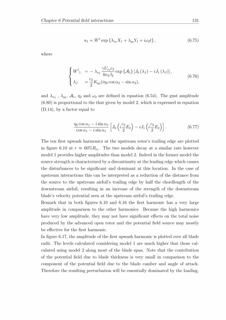
Chapter 6 Potential field interactions 131
u1 = W l exp λx2X1 + λy2Y1 + iω2t , (6.75)
where
W l
1 = − λx2
γUr2c2
4n2β2
exp A1 [J0 (λJ)− iJ1 (λJ)] ,
λJ =c2
2Ky2(iη2 cosα2 − sinα2),
(6.76)
and λx2 , λy2 , A1, η2 and ω2 are defined in equation (6.54). The gust amplitude
(6.80) is proportional to the that given by model 2, which is expressed in equation
(D.14), by a factor equal to
η2 cosα1 − i sinα1
cosα1 − i sinα1
[J0
(ic2
2E2
)− iJ1
(ic2
2E2
)]. (6.77)
The ten first upwash harmonics at the upstream rotor’s trailing edge are plotted
in figure 6.10 at r ≈ 60%Rt1 . The two models decay at a similar rate however
model 1 provides higher amplitudes than model 2. Indeed in the former model the
source strength is characterized by a discontinuity at the leading edge which causes
the disturbances to be significant and dominant at this location. In the case of
upstream interactions this can be interpreted as a reduction of the distance from
the source to the upstream airfoil’s trailing edge by half the chordlength of the
downstream airfoil, resulting in an increase of the strength of the downstream
blade’s velocity potential seen at the upstream airfoil’s trailing edge.
Remark that in both figures 6.10 and 6.16 the first harmonic has a very large
amplitude in comparison to the other harmonics. Because the high harmonics
have very low amplitude, they may not have significant effects on the total noise
produced by the advanced open rotor and the potential field source may mostly
be effective for the first harmonic.
In figure 6.17, the amplitude of the first upwash harmonic is plotted over all blade
radii. The levels calculated considering model 1 are much higher that those cal-
culated using model 2 along most of the blade span. Note that the contribution
of the potential field due to blade thickness is very small in comparison to the
component of the potential field due to the blade camber and angle of attack.
Therefore the resulting perturbation will be essentially dominated by the loading.
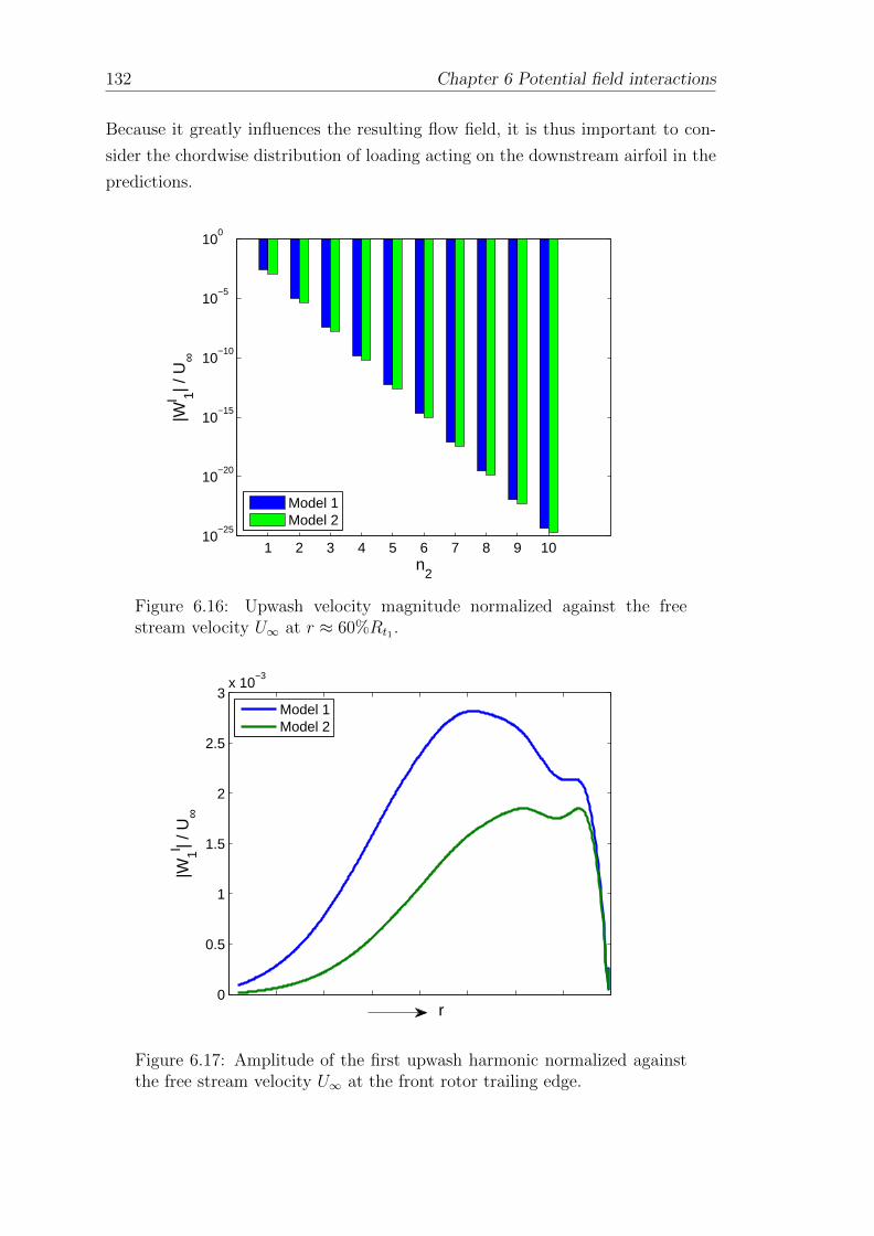
132 Chapter 6 Potential field interactions
Because it greatly influences the resulting flow field, it is thus important to con-
sider the chordwise distribution of loading acting on the downstream airfoil in the
predictions.
1 2 3 4 5 6 7 8 9 1010
−25
10−20
10−15
10−10
10−5
100
n2
|Wl 1| /
U∞
Model 1Model 2
Figure 6.16: Upwash velocity magnitude normalized against the freestream velocity U∞ at r ≈ 60%Rt1 .
0
0.5
1
1.5
2
2.5
3x 10
−3
r
|W1l | /
U∞
Model 1Model 2
Figure 6.17: Amplitude of the first upwash harmonic normalized againstthe free stream velocity U∞ at the front rotor trailing edge.

Chapter 6 Potential field interactions 133
The total amplitude of the gust incident on the upstream airfoil is the sum of the
gust amplitudes of the thickness and the loading components, which are defined
in equations (6.54) and (6.80). The evolution of the “total” upwash velocity in
the inter-rotor region is assessed in figure 6.18 in which the amplitude of the first
upwash harmonic provided by the two analytical models is compared with the CFD
data at various axial locations at r ≈ 60%Rt1 . Both the analytical models and the
CFD results show evidence of the exponential decay of the velocity potential with
axial distance in most of the inter-rotor region. Nevertheless the CFD exhibits
a notable drop in the gust amplitude close to the upstream airfoil’s trailing edge
which could be due to interactions with the complex flow field surrounding the
blade. The numerical simulation also displays a discontinuity which is in fact
located at the position of the sliding plane. Particularly, it is clear in figure
6.19 that the upwash velocities measured one cell upstream and downstream of
the sliding plane both differ in phase and amplitude. Those disparities could be
caused by several sources such as numerical dissipation across the sliding plane
due to the interpolated mesh, difficulties numerically capturing the features of
the flow between the contra-rotative blade rows at the sliding plane, difficulties
extracting the bound potential field of the downstream rotor at either side of the
sliding plane, or the different extraction procedures upstream and downstream of
the sliding plane (such as time averaging in different frames or reference).
1 1.5 2 2.5 3 3.510
−3
10−2
10−1
100
2 x1/c
1
|Un|/U
∞
CFDModel 1 − Geometry BModel 2 − Geometry B
Figure 6.18: Amplitude of the first upwash harmonic normalized againstthe free stream velocity U∞ in the inter-rotor region. The analytical modelsare compared with the CFD data.
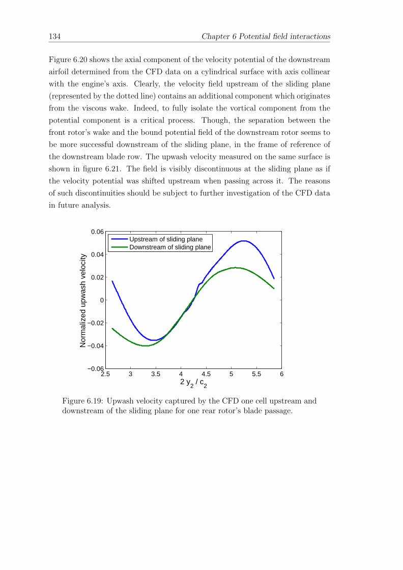
134 Chapter 6 Potential field interactions
Figure 6.20 shows the axial component of the velocity potential of the downstream
airfoil determined from the CFD data on a cylindrical surface with axis collinear
with the engine’s axis. Clearly, the velocity field upstream of the sliding plane
(represented by the dotted line) contains an additional component which originates
from the viscous wake. Indeed, to fully isolate the vortical component from the
potential component is a critical process. Though, the separation between the
front rotor’s wake and the bound potential field of the downstream rotor seems to
be more successful downstream of the sliding plane, in the frame of reference of
the downstream blade row. The upwash velocity measured on the same surface is
shown in figure 6.21. The field is visibly discontinuous at the sliding plane as if
the velocity potential was shifted upstream when passing across it. The reasons
of such discontinuities should be subject to further investigation of the CFD data
in future analysis.
2.5 3 3.5 4 4.5 5 5.5 6−0.06
−0.04
−0.02
0
0.02
0.04
0.06
2 y2 / c
2
Nor
mal
ized
upw
ash
velo
city
Upstream of sliding planeDownstream of sliding plane
Figure 6.19: Upwash velocity captured by the CFD one cell upstream anddownstream of the sliding plane for one rear rotor’s blade passage.

Chapter 6 Potential field interactions 135
Figure 6.20: Axial component of the downstream airfoil’s velocity potentialnormalized against the free-stream velocity captured by the CFD at r ≈60%Rt1 in the inter-rotor region.
Figure 6.21: Upwash velocity normalized against the free-stream velocitycaptured by the CFD at r ≈ 60%Rt1 in the inter-rotor region.

136 Chapter 6 Potential field interactions
6.2.3 Response of the upstream airfoil
This section refers to the high frequency response of the upstream airfoil to the
potential field of the adjacent blade. The latter being decomposed into thickness
and lift contributions, the resultant upwash on the upstream airfoil is the linear
sum of these different components. The expression used in this section was derived
by Parry for a semi-infinite flat plate, extending to upstream infinity, using the
Wiener-Hopf technique. Since the trailing edge problem is considered, the Kutta
condition was imposed at the trailing edge of the upstream airfoil. This repre-
sentation nonetheless neglects the inverse square root singularity at the leading
edge where the pressure tends to infinity. Parry (1988) showed that in the case of
incompressible flow, neglecting the leading edge effects led to errors in the determi-
nation of the unsteady pressure, but that in the compressible flow case the leading
edge correction had relatively small impact on the total airfoil response. However,
it has been decided that any singularity be addressed, therefore the leading edge
correction will be applied to the semi-infinite response. The latter is given by
(Parry, 1988, equation 7.4.48)
∆p(X1) = − i 2ρUr1W1(σ − µ)
β10.5(iσ∗ + iµ)0.5(i σ − iµ)0.5
[exp
iσ∗(X1 − 1)w[i ((1−X1)(iµ+ iσ∗))0.5]
− exp −iµ(X1 − 1)] exp iω2t . (6.78)
where the function w is defined by (Abramowitz and Stegun, 1964, equation 7.1.3)
as
w(z) = exp−z2
erfc(−iz), (6.79)
and
W1 =W t1 +W l
1,
σ =kc1
2Mr1
,
σ =Mr1
1 +Mr1
σ,
σ∗ =σMr1
1−Mr1
,
k =ω2
c0
,
µ = iλx2
c1
2.
(6.80)

Chapter 6 Potential field interactions 137
The acoustically weighted lift per unit span is obtained by integrating the pressure
over the blade chord, including the non-compactness factor exp
−ikX
2X1
c1
and
is given by Parry by
dL1
dr=
ρUr1c1(σ − µ) exp iω2t− ikX(1−Mr1
2)0.5(µ+ kX)(iµ+ iσ∗)0.5(iσ − iµ)0.5
[− exp i2(µ+ kX)
+ w[i(2(iµ+ iσ∗))0.5
]+ exp
−iπ
4
(iµ+ iσ∗)0.5
(σ∗ − kX)0.5
×
(1− exp −i2(σ∗ − kX)w
[(i− 1)(σ∗ − kX)0.5
])].
(6.81)
To account for the leading edge effects, Parry introduced a correction term based
on a technique developed by Landahl (1989) and Adamczyk (1971). The pressure
jump associated with the leading edge contribution was given by
∆pLE(X1) =
(2
π
)0.5iρW1Ur1(σ − µ) exp iω2t+ iσ(1−X1)− 4iσ
(iµ+ iσ∗)(iσ − iµ)0.5(1−Mr22)0.5
×[
w[− exp
−iπ
4
(2σ(1 +X1))0.5
]−(
2
πσ′′(1 +X1)
)0.5
exp−iπ
4
].
(6.82)
where
σ =
σMr1
1−M2r1
,
σ′′
=1 +Mr1
Mr1(1−Mr1)σ.
(6.83)
The lift per unit span associated with the leading edge term is given by (Parry,
1988, equation 7.5.12),
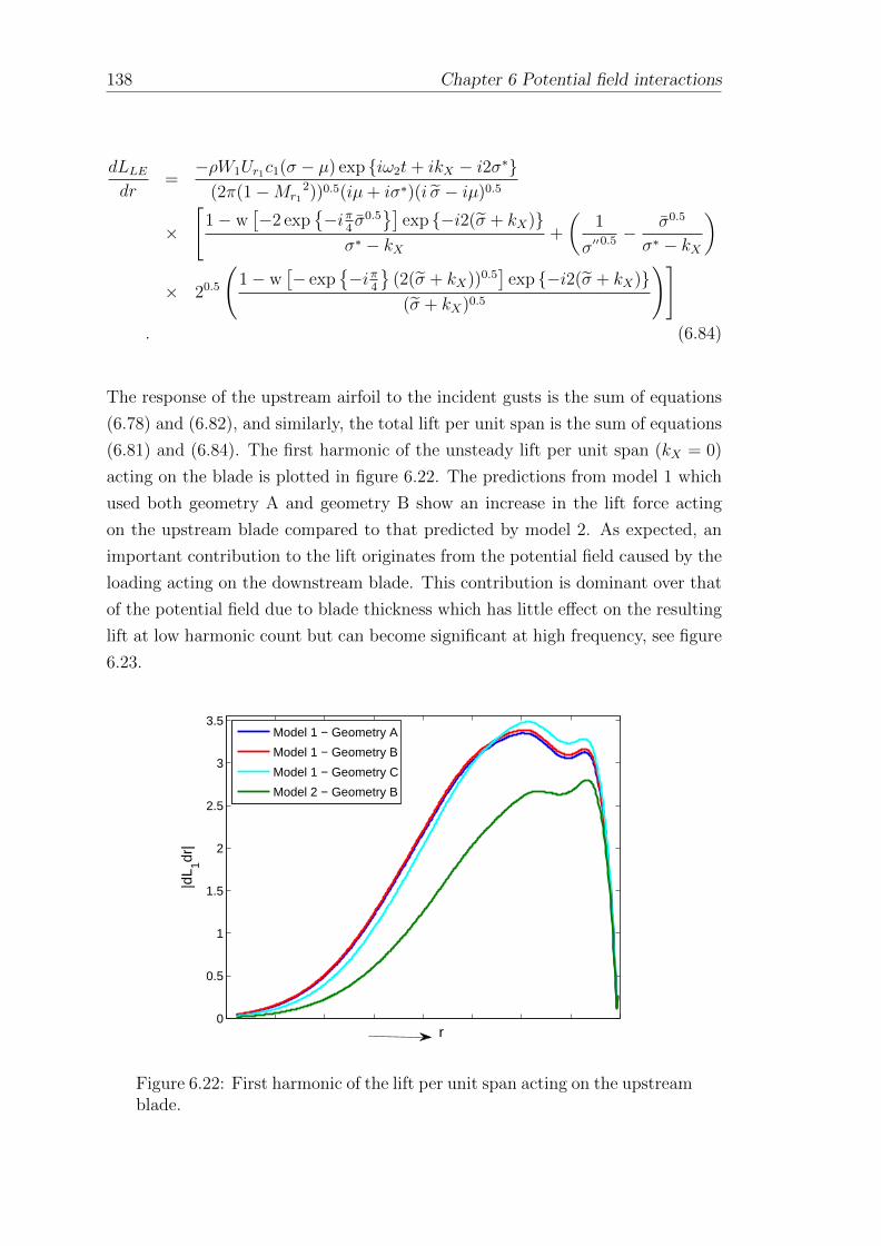
138 Chapter 6 Potential field interactions
dLLEdr
=−ρW1Ur1c1(σ − µ) exp iω2t+ ikX − i2σ∗
(2π(1−Mr12))0.5(iµ+ iσ∗)(i σ − iµ)0.5
×[
1− w[−2 exp
−iπ
4σ0.5]
exp −i2(σ + kX)σ∗ − kX
+
(1
σ′′0.5− σ0.5
σ∗ − kX
)
× 20.5
(1− w
[− exp
−iπ
4
(2(σ + kX))0.5
]exp −i2(σ + kX)
(σ + kX)0.5
)]. (6.84)
The response of the upstream airfoil to the incident gusts is the sum of equations
(6.78) and (6.82), and similarly, the total lift per unit span is the sum of equations
(6.81) and (6.84). The first harmonic of the unsteady lift per unit span (kX = 0)
acting on the blade is plotted in figure 6.22. The predictions from model 1 which
used both geometry A and geometry B show an increase in the lift force acting
on the upstream blade compared to that predicted by model 2. As expected, an
important contribution to the lift originates from the potential field caused by the
loading acting on the downstream blade. This contribution is dominant over that
of the potential field due to blade thickness which has little effect on the resulting
lift at low harmonic count but can become significant at high frequency, see figure
6.23.
0
0.5
1
1.5
2
2.5
3
3.5
r
|dL 1dr
|
Model 1 − Geometry A
Model 1 − Geometry B
Model 1 − Geometry C
Model 2 − Geometry B
Figure 6.22: First harmonic of the lift per unit span acting on the upstreamblade.

Chapter 6 Potential field interactions 139
0
1
2
3
4
5
6
7x 10
−8
r
|dL 1dr
|
Model 1 − Geometry AModel 1 − Geometry BModel 1 − Geometry CModel 2 − Geometry B
Figure 6.23: Fifth harmonic of the lift per unit span acting on the upstreamblade.
A comparison of the analytical methods with the CFD simulation was conducted.
The comparisons show a reasonable agreement for the first harmonic in terms of
upwash velocity and lift per unit span, as shown in figures 6.18 and 6.24 respec-
tively. However the agreement becomes very poor at higher harmonics. In figure
6.25 a comparison between the magnitude of the first three harmonics of the vis-
cous wake and the potential field contributions extracted from the CFD data in
the inter-rotor region is shown. Upstream of the sliding plane, only the first up-
wash harmonic related to the potential field was captured properly in the CFD
simulation. Significant errors are observed for the second and third harmonics
in this region, underlining difficulties separating the potential field contribution
from the numerical solution in the given frame of reference. The results are also
strongly affected by the discontinuity at the sliding plane. However, the potential
field is perfectly captured close to the downstream blade row. Thus the use of
the analytical model would be a useful asset to calculate the related perturbation
at the upstream blade’s trailing edge avoiding those numerical errors. Note that
the viscous wake contribution is also subject to discontinuities at the sliding plane
and inaccuracies downstream of the sliding plane. The origin of those inaccuracies
should be investigated further to determine if they are a numerical artefact or the
result of some non-linear interaction between both fields. It is interesting to notice
that in the analysis of Jaron et al. (2014) the amplitude of the Fourier harmonics

140 Chapter 6 Potential field interactions
of the simulated velocity field also showed a decreasing then increasing behaviour
at some axial locations.
0
0.5
1
1.5
2
2.5
3
3.5
r
|dL 1dr
|
Model 1 − Geometry B
Model 2 − Geometry B
CFD
Figure 6.24: Comparison between the first harmonic of the lift per unitspan acting on the upstream blade provided by the analytical models andthe CFD.
1 1.5 2 2.5 3 3.5 410
−4
10−3
10−2
10−1
100
2 x1 / c
1
|Un| /
U∞
Rear Pot n
2 = 1
Wake − n1 = 1
Rear Pot n2 = 2
Wake n1 = 2
Rear Pot n2 = 3
Wake n1 = 3
Sliding plane
Figure 6.25: Amplitude of the first three upwash harmonics determinedfrom the CFD data.
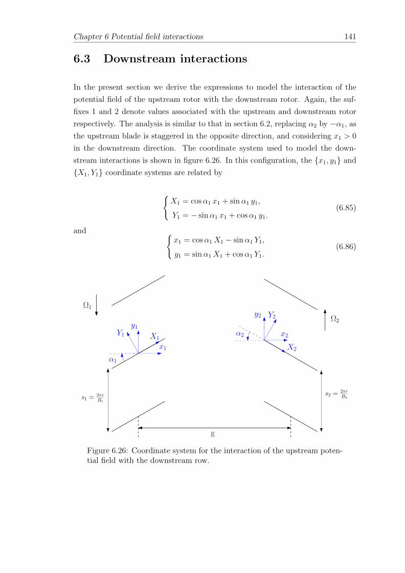
Chapter 6 Potential field interactions 141
6.3 Downstream interactions
In the present section we derive the expressions to model the interaction of the
potential field of the upstream rotor with the downstream rotor. Again, the suf-
fixes 1 and 2 denote values associated with the upstream and downstream rotor
respectively. The analysis is similar to that in section 6.2, replacing α2 by −α1, as
the upstream blade is staggered in the opposite direction, and considering x1 > 0
in the downstream direction. The coordinate system used to model the down-
stream interactions is shown in figure 6.26. In this configuration, the x1, y1 and
X1, Y1 coordinate systems are related by
X1 = cosα1 x1 + sinα1 y1,
Y1 = − sinα1 x1 + cosα1 y1.(6.85)
and x1 = cosα1X1 − sinα1 Y1,
y1 = sinα1X1 + cosα1 Y1.(6.86)
X1Y1
x1
x2
Y2
X2
α1
α2
y1
y2Ω1
Ω2
g
s2 =2πrB2s1 =
2πrB1
Figure 6.26: Coordinate system for the interaction of the upstream poten-tial field with the downstream row.

142 Chapter 6 Potential field interactions
6.3.1 Potential field due to blade thickness
6.3.1.1 Velocity potential of the upstream airfoil
Isolated airfoil. We consider an isolated airfoil of the upstream row. The non-
dimensional thickness function G(X1) is expressed as
G(X1) = sin
(π
2Xm
(X1 +
c1
2
))if − c1
2< X1 < −
c1
2+Xm,
G(X1) = sin
(π
2+π
2
X1 + c12−Xm
c1 −Xm
)if − c1
2+Xm < X1 <
c1
2.
(6.87)
The thickness effects are thus modelled by a distribution of sources of strength f t
which is given by
f t(X1) =
Ur1tmaxπ
2β1Xm
cos
(π
2Xm
(X1 +
c1
2
))if − c1
2< X1 < −
c1
2+Xm,
f t(X1) = − Ur1tmaxπ
2β1(c1 −Xm)sin
(π
2
X1 + c1/2−Xm
c1 −Xm
). if − c1
2Xm < X1 <
c1
2,
(6.88)
where Xm is now the local chordwise coordinate of the point of maximum thickness
tmax of the upstream airfoil, and β1 =√
1−Mr12. The potential of a point source
located at χ1 = Xs and ζ1 = 0 satisfies the following governing equation and
boundary condition
β12 ∂
2ϑt
∂X12 +
∂2ϑt
∂Y12 = β1δ (X1 −Xs) δ(Y1), (6.89)
limY1→0±
∂φt
∂Y1
(−c1
2< X1 <
c1
2, Y1
)= ±Ur1
tmax2
∂G∂X1
, (6.90)
An elementary singular solution to equation (6.90) is
ϑt((X1, Y1)|(Xs, 0)) =1
2πlog
(1
β1
√(X1 −Xs)2 + β1
2Y12
). (6.91)
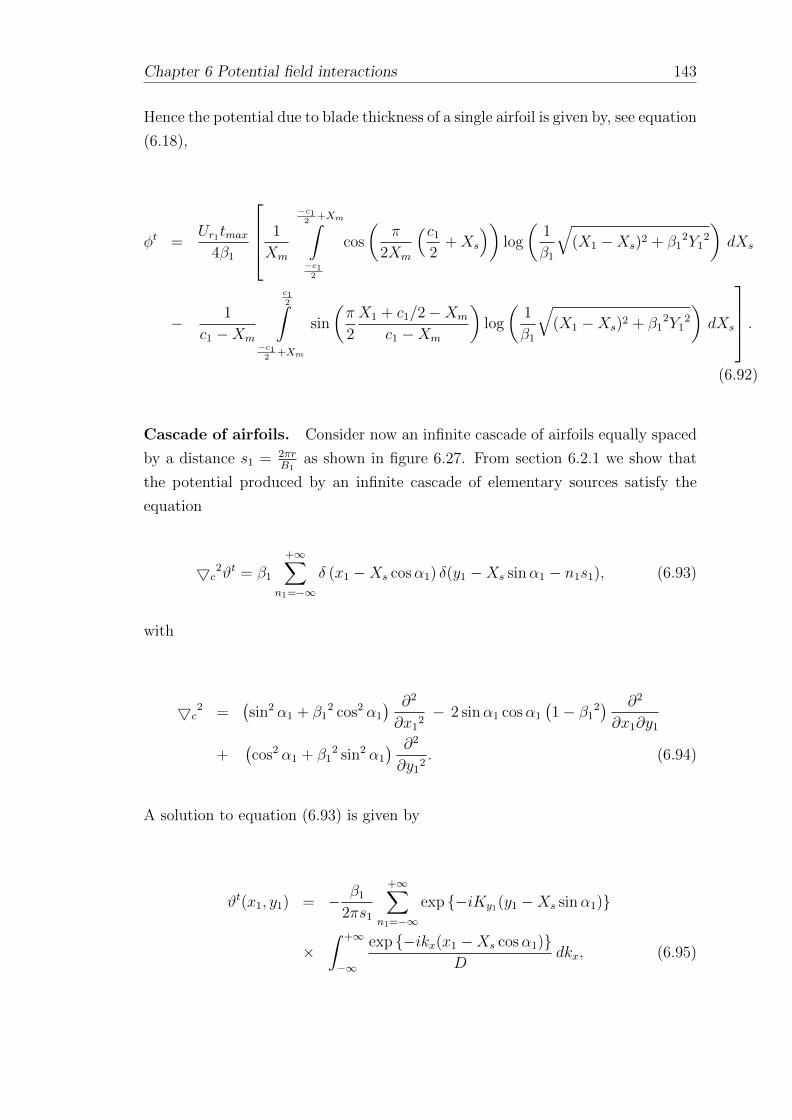
Chapter 6 Potential field interactions 143
Hence the potential due to blade thickness of a single airfoil is given by, see equation
(6.18),
φt =Ur1tmax
4β1
1
Xm
−c12
+Xm∫−c1
2
cos
(π
2Xm
(c1
2+Xs
))log
(1
β1
√(X1 −Xs)2 + β1
2Y12
)dXs
− 1
c1 −Xm
c12∫
−c12
+Xm
sin
(π
2
X1 + c1/2−Xm
c1 −Xm
)log
(1
β1
√(X1 −Xs)2 + β1
2Y12
)dXs
.(6.92)
Cascade of airfoils. Consider now an infinite cascade of airfoils equally spaced
by a distance s1 = 2πrB1
as shown in figure 6.27. From section 6.2.1 we show that
the potential produced by an infinite cascade of elementary sources satisfy the
equation
5c2ϑt = β1
+∞∑n1=−∞
δ (x1 −Xs cosα1) δ(y1 −Xs sinα1 − n1s1), (6.93)
with
5c2 =
(sin2 α1 + β1
2 cos2 α1
) ∂2
∂x12− 2 sinα1 cosα1
(1− β1
2) ∂2
∂x1∂y1
+(cos2 α1 + β1
2 sin2 α1
) ∂2
∂y12. (6.94)
A solution to equation (6.93) is given by
ϑt(x1, y1) = − β1
2πs1
+∞∑n1=−∞
exp −iKy1(y1 −Xs sinα1)
×∫ +∞
−∞
exp −ikx(x1 −Xs cosα1)D
dkx, (6.95)
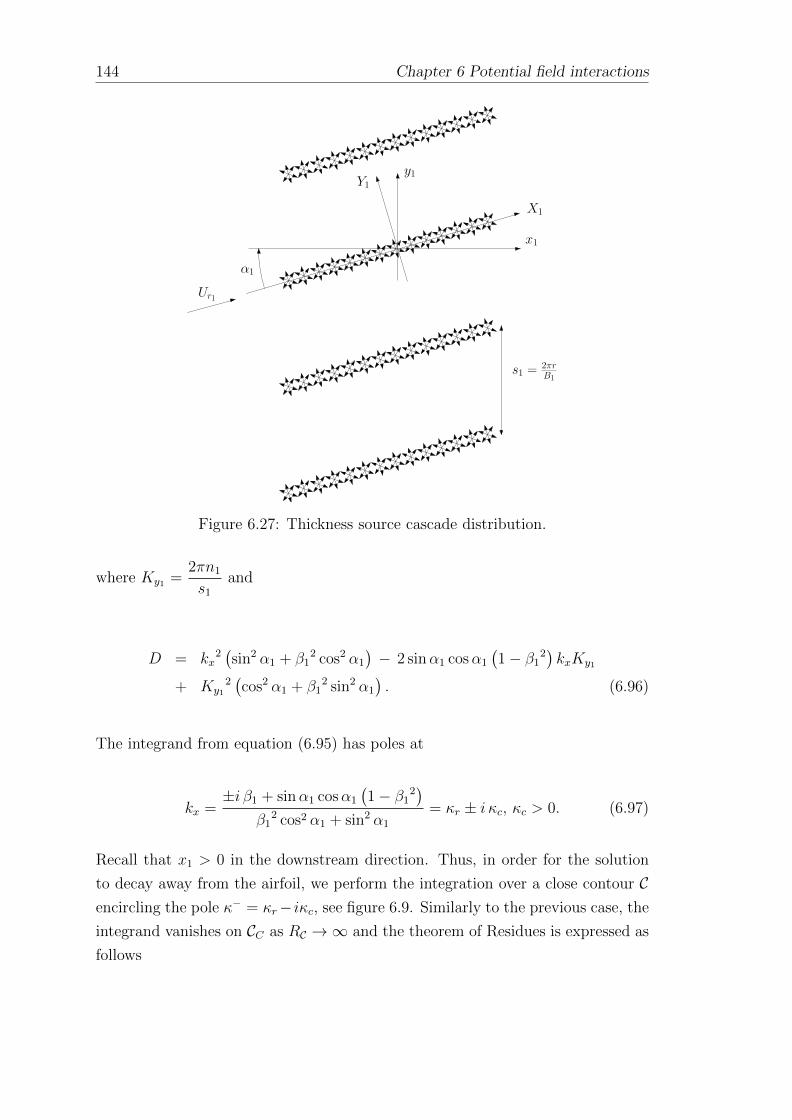
144 Chapter 6 Potential field interactions
Y1
X1
s1 =2πrB1
y1
x1
α1
Ur1
Figure 6.27: Thickness source cascade distribution.
where Ky1 =2πn1
s1
and
D = kx2(sin2 α1 + β1
2 cos2 α1
)− 2 sinα1 cosα1
(1− β1
2)kxKy1
+ Ky1
2(cos2 α1 + β1
2 sin2 α1
). (6.96)
The integrand from equation (6.95) has poles at
kx =±i β1 + sinα1 cosα1
(1− β1
2)
β12 cos2 α1 + sin2 α1
= κr ± i κc, κc > 0. (6.97)
Recall that x1 > 0 in the downstream direction. Thus, in order for the solution
to decay away from the airfoil, we perform the integration over a close contour Cencircling the pole κ− = κr− iκc, see figure 6.9. Similarly to the previous case, the
integrand vanishes on CC as RC →∞ and the theorem of Residues is expressed as
follows

Chapter 6 Potential field interactions 145
∮CR
exp −ikx(x1 −Xs cosα1)D
dkx = −2πiResκ−
(exp −ikx(x1 −Xs cosα1)
D
).
(6.98)
−Ky
Ky
Re(kx)
Im(kx)
Cc
Cr−RC RC
Figure 6.28: Contour integration.
Note that the negative sign at the left hand side of equation (6.98) is due to the
fact that the outer circle CC is going clockwise around κ−.
The potential field due to blade thickness produced by a unit strength elementary
source is thus
ϑt(x1, y1) = − 1
2s1
+∞∑n1=−∞
1
Ky1
exp −Ky1(µ1 + iµ2)(x1 −Xs cosα1)− iKy1(y1 −Xs sinα1) ,
(6.99)
where
µ1 =β1
β12 cos2 α1 + sin2 α1
, µ2 =sinα1 cosα1(1− β1
2)
β12 cos2 α1 + sin2 α1
. (6.100)
The analytical expression of the potential follows immediately as
φt = −Ur1tmaxπ4β1s1
+∞∑n1=−∞
1
Ky1
exp −Ky1η1x1 − iKy1y1 [I1 + I2] , (6.101)
where η1 = (µ1 + i µ2), and I1 and I2 are expressed as
146 Chapter 6 Potential field interactions
I1 =1
Xm
−c12
+Xm∫−c1
2
cos
(π
2Xm
(Xs +
c1
2
))exp Ky1 [η1 cosα1 + i sinα1]Xs dXs, (6.102)
I2 = − 1
c1 −Xm
c12∫
−c12
+Xm
sin
(π
2
Xs + c1/2−Xm
c1 −Xm
)exp Ky1 [η1 cosα1 + i sinα1]Xs dXs.
The above integrals are equal to
I1 =2 exp
−E1
(c12−Xm
)[π − 2E1Xm exp −E1Xm]
π2 + 4E12X2
m
, (6.103)
I2 = −2[π exp
E1
(− c1
2+Xm
)+ 2 exp
c12E1
(c1 −Xm)E1
]π2 + 4E1
2(c1 −Xm)2, (6.104)
where
E1 = Ky1 [η1 cosα1 + i sinα1] . (6.105)
6.3.1.2 Upwash on the downstream airfoil
Now consider an isolated airfoil of the downstream row in the coordinate system
shown in figure 6.26. The upwash normal to such airfoil is given by
u2 = sinα2∂φt
∂x1
− cosα2∂φt
∂y1
, (6.106)
where α2 is the local stagger angle of the downstream airfoil. Applying the above
equation to equation (6.101) yields
u2 = −Ur2tmaxπ4s2β2
[−η1 sinα2+i cosα2] exp −Ky1η1x1 − iKy1y1 [I1 + I2] . (6.107)
The x1, y1 and x2, y2 coordinate systems defined in figure 6.26 are related by

Chapter 6 Potential field interactions 147
x1 = x2 + g − c2
2cosα2,
y1 = y2 +c2
2sinα2 + r(Ω1 + Ω2)t. (6.108)
Inserting equation (6.108) into equation (6.107) and expressing the upwash in
terms of X2, Y2 coordinates using equation (6.21), one harmonic of the upwash
normal to the reference airfoil of the downstream row can be written of the form
u2 = W t2 exp λx1X2 + λy1Y2 − iω1t , (6.109)
where
W t2 = − λ∗y1
Ur1tmax8n1β1
exp A2 [I1 + I2] ,
A2 = −Ky1
(η1
(g − c2
2cosα2
)+ i
c2
2sinα2
),
λx1 =− Ky1(η1 cosα2 − i sinα2),
λy1 = −Ky1(η1 sinα2 + i cosα2),
ω1 =Ky1r(Ω1 + Ω2).
(6.110)
The term λ∗y1 corresponds to the conjugate of λy1 . The magnitude of the first
harmonic of the upwash velocity incident on the downstream airfoil’s leading edge
calculated using models 1 and 2 is shown in figure 6.29. In the latter, geometry A
refers to the profile represented by the thickness function defined in equation (6.87)
and geometry B corresponds to that of an ellipse. On the determination of the
potential field of an ellipse, the consideration of the thickness distribution along the
chordline provides greater amplitudes than the point source representation. Recall
that the point source representation is a far-field approximation thus the distance
between the two blade rows should be large enough for the models to converge.
It is interesting to observe that in the present case the change of geometry has a
notable influence on the amplitudes predicted by model 1, causing a difference of
approximately 22 % in the peak amplitude of the upwash harmonic. This increase
is essentially due to the fact that the the thickness distribution of the elliptic
profile is defined over a wider area (with, in particular, a blunt trailing edge) and
has its point of maximum thickness closer to the downstream airfoil than the one
of geometry A. The amplitude of the fifth harmonic of the upwash incident on the
148 Chapter 6 Potential field interactions
downstream airfoil is plotted in figure 6.30. Again, the source representation and
the type of profile considered strongly influences the solution.
0
0.5
1
1.5x 10
−4
r
|W1t | /
U∞
Model 1 − Geometry AModel 1 − Geometry BModel 2 − Geometry B
Figure 6.29: Amplitude of the first upwash harmonic normalized againstthe free stream velocity at the downstream blade’s leading edge (thicknesscontribution).
0
0.5
1
1.5
2
2.5
3
3.5
4
4.5
x 10−14
r
|W1t | /
U∞
Model 1 − Geometry AModel 1 − Geometry BModel 2 − Geometry B
Figure 6.30: Amplitude of the fifth upwash harmonic normalized againstthe free stream velocity at the downstream blade’s leading edge (thicknesscontribution).

Chapter 6 Potential field interactions 149
6.3.2 Potential field due to blade circulation
6.3.2.1 Velocity potentials of the upstream airfoil and of the cascade
The velocity potential of the upstream airfoil is obtained using the same method
as in section 6.2.2, using the coordinates associated with the upstream airfoil with
x1 > 0 in the upstream direction and replacing α2 by −α1. The source strength
is given by
f l(X1) = −2γUr1β1
√c1 −X1
X1
. (6.111)
The stream function for a cascade of distribution of elementary sources is obtained
by applying the theorem of Residues as in equation (6.98), performing the kx-
integral over the close contour C defined in figure 6.28
ϑl(x1, y1) = − 1
2s1
+∞∑n1=−∞
1
Ky1
exp −Ky1η1(x1 −Xs cosα1)− iKy1(y1 −Xs sinα1) ,
(6.112)
and the stream function associated with the distribution of sources of strength f l
is given by
ψl =πγUr1β1s1
c1
2
+∞∑n1=−∞
exp −Ky1η1x1 − iKy1y1Ky1
×[J0
(Ky1
c1
2[−iη1 cosα1 + sinα1]
)− iJ1
(Ky1
c1
2[−iη1 cosα1 + sinα1]
)].
(6.113)
6.3.2.2 Upwash on the downstream airfoil
Consider an isolated airfoil from the upstream blade row in the coordinate system
defined by figure 6.26. Using the same method as in section 6.3.1.2, the upwash
normal to the downstream blade is given by

150 Chapter 6 Potential field interactions
u2 = W l2 exp λx1X2 + λy2Y2 + iω1t , (6.114)
where
W l
2 = − λx1
γUr1c1
4n1β1
exp A2 [J0(λJ1)− iJ1(λJ1)] ,
λJ1 =Ky1
c1
2(−iη1 cosα1 + sinα1) ,
(6.115)
and A2, λy1 , and λx1 are defined in equation (6.110).
Figure 6.31 shows the magnitude of the first upwash harmonic calculated along the
downstream blade’s leading edge. As observed in section 6.2.2, there are signifi-
cant differences in amplitude between the results provided by model 1 and those
provided by model 2. In the case of downstream interactions the latter produces
stronger perturbations at the vicinity of the downstream row than the former.
This trend is expected owing to the fact that the point source is defined at the
upstream airfoil’s midchord whereas in the distributed profile the dominant source
is located at the leading edge. Because the velocity potential decays exponentially
with axial distance the difference in the source representation has a great influence
on the predicted levels.
6.3.3 Response of the downstream airfoil
Since we now consider the response of the downstream airfoils to the unsteady
perturbations produced by the upstream row, the airfoil response is expected to
be dominated by the leading edge singularity. Parry derived another expression to
treat only the leading edge problem under the assumption that the trailing edge
region is negligible, leading to the following solution.
∆p(X2) =−2ρW2Ur2 exp iω1t
(1−Mr22)0.5(iµ+ iσ∗)0.5
[(exp −i σ(X2 + 1)w
[i(X2 + 1)0.5(−iµ+ i σ)0.5
]− exp −iµ(X2 + 1)) i(σ − µ)
(−iµ+ i σ)0.5− exp −i σ(X2 + 1)
π0.5(X2 + 1)0.5
], (6.116)

Chapter 6 Potential field interactions 151
0
1
2
x 10−4
r
|W1l | /
U∞
Model 1Model 2
Figure 6.31: Amplitude of the first upwash harmonic (loading contribu-tion) normalized against the free stream velocity at the downstream blade’sleading edge.
where
W2 =W t2 +W l
2,
σ =kc2
Mr2
,
σ =Mr2
1 +Mr2
σ,
σ∗ =σMr2
1−Mr2
,
k =ω1
c0
,
µ = iλx2
c2
2.
(6.117)
Again, the lift per unit span is obtained by integrating the above equation over
the chord accounting for the non-compactness factor. This yields
152 Chapter 6 Potential field interactions
dL2
dr=
ρW2Ur2c2 exp ikX + iω1t(1−Mr2
2)0.5(iµ+ iσ∗)0.5(µ+ kX)
×[
exp−iπ
4
(σ + kX)
(σ + kX)0.5
(1− w
[−(1− i)(σ + kX)0.5
]exp −i2(σ + kX)
)+
σ − µ(i σ − iµ)0.5
(w[i20.5(i σ − iµ)0.5
]exp −2i(σ + kX) − exp −i2(µ+ kX)
)].
(6.118)
The lift per unit span calculated at the downstream blade’s radius range is shown
in figure 6.32. It is observed in this case that, because the potential field due to
the blade loading is weaker, the airfoil’s geometry has greater influence on the
resulting lift in comparison to the upstream interaction case.
0
0.1
0.2
0.3
0.4
r
|dL 1dr
|
Model 1 − Geometry AModel 1 − Geometry BModel 2 − Geometry B
Figure 6.32: First harmonic of the lift per unit span acting on the down-stream blade.

Chapter 6 Potential field interactions 153
6.4 Potential field interaction noise prediction
The radiated noise caused by the interaction between the potential field of one ro-
tor and the adjacent rotor was calculated using the radiation formula from equation
(4.36). The polar directivity of different interaction tones was investigated and the
contributions of the forward and rearward potential fields were compared to that
of the viscous wakes. The analysis also included a brief comparison between the
noise levels calculated by model 1 and model 2. Finally, a cross-validation of the
analytical models with wind tunnel measurements and CFD-based noise predic-
tions was conducted. In this section the forward potential refers to the interaction
between the potential field of the downstream rotor with the upstream row, and
the rearward potential refers to the interaction between the potential field of the
upstream rotor with the downstream row. Note that, unless otherwise specified,
the results presented in the following used the geometry B.
The relative contributions of the wake and of the rotors’ potential field to the
sound pressure level of the first interaction tone 1, 1 are shown in figure 6.33
for a given take-off case. The wake interaction noise evidently constitutes the
principal source of tonal noise. Nevertheless the forward potential appears to
be dominant at some observer locations. The addition of the contribution of the
forward potential provides a better agreement with the wind tunnel measurements
at those particular locations. In this case the rearward potential has no effect on
the emitted noise.
As mentioned in section 6.2.2.2 the potential field due to blade thickness is likely
to have little effect on the first interaction tone produced by the potential field
interactions. In the given take-off case the change of geometry in model 1 only
engender differences in sound pressure levels up to around 1.5dB for the upstream
interactions and up to approximately 3dB for downstream interactions at few
observer locations, see figure 6.34.
A comparison between the noise levels predicted by model 1 and model 2 is shown
in figure 6.35 for the tone 1, 1. As a logical continuation of previous observa-
tions, model 1 produces higher noise levels than model 2 in the case of upstream
interactions, and lower levels in the case of downstream interactions. Differences
from 2dB to about 8dB are observed between the results from the two methods.
The use of a distributed source model could thus have non negligible effect on the
predicted noise levels at some observer locations if the potential field interaction
becomes a predominant source of tonal noise.

154 Chapter 6 Potential field interactions
20 40 60 80 100 120 140 160Polar emission angle (°)
SP
L
MeasurementsWake − Analytical modelForward potential − Model 1Rearward potential − Model 1Total − Analytical model
10 dB
Figure 6.33: Relative contribution of the potential field and viscous wakeeffects for the polar directivity of the tone 1, 1 compared with windtunnel measurements and CFD-based calculations at a given take-off case.
20 40 60 80 100 120 140 160Polar emission angle (°)
SP
L (d
B)
Forward potential − Model 1, Geometry BForward potential − Model 1, Geometry AForward potential − Model 1, Geometry CRearward potential − Model 1, Geometry BRearward potential − Model 1, Geometry A
10 dB
Figure 6.34: Effect of the airfoil’s geometry on the polar directivity of thetone 1, 1 caused by potential field interactions.
The predictions performed using the CFD blade response in the analytical noise
Chapter 6 Potential field interactions 155
radiation formulae were also compared with the analytical model in figure 6.35
for the case of upstream interactions. There is a good agreement between the
CFD-based calculation and both analytical models at most of the emission polar
angles. In figure 6.36 the sum of the contributions from the viscous wake and the
downstream rotor’s potential field provided by the CFD-based calculations and
by model 1 are compared with wind tunnel measurements. Both methods show a
reasonable agreement with the measurements in terms of absolute levels within a
range of 10dB at most observer locations. Yet some more important discrepancies
between the predicted and measured levels (≈ 15dB) remain present, in particular
between 110 and 115. Note that the analytical model does not take into account
other flow disturbances that could influence the results such as the swirl or induced
velocity in the inter-rotor region, the tip of hub vortices or the interactions between
the blades of the same row or between the flow velocity fields. The results could
also be affected by measurements uncertainties or numerical dissipation in the
CFD simulation. Nonetheless the noise levels provided by each method lie in the
same ballpark thus prove to be promising for future studies.
20 40 60 80 100 120 140 160Polar emission angle (°)
SP
L
Forward potential − Model 1Forward potential − Model 2Forward potential − CFDRearward potential − Model 1Rearward potential − Model 2
10 dB
Figure 6.35: Polar directivity of the tone 1, 1 due to the potential fieldinterractions calculated using analytical models and the CFD blade re-sponse.

156 Chapter 6 Potential field interactions
20 40 60 80 100 120 140 160Polar emission angle (°)
SP
L
MeasurementsTotal − Analytical modelTotal − CFD
10 dB
Figure 6.36: Polar directivity of the tone 1, 1 due to the potential fieldand wake interractions calculated using model 1 and the CFD blade re-sponse compared with wind tunnel measurements.
The polar directivity of the tone 1, 2 is shown in figure 6.37 and is decomposed
into the different contributions from the interaction sources of interest. As ex-
pected the potential field interactions have no effect on the emitted noise levels
due to the small order of magnitude of the perturbations. Although it is interest-
ing to note that in this case the effect of the rearward potential becomes dominant
other that of the forward potential downstream of the engine.

Chapter 6 Potential field interactions 157
40 80 120 160Polar emission angle (°)
SP
L
Measurements
Wake − Analytical model
Wake − CFD
Rearward potential − Model 1
Rearward potential − Model 2
Forward potential − Model 1
Forward potential − Model 2
20 dB
Figure 6.37: Relative contribution of the potential field and viscous wakeeffects for the polar directivity of the tone 1, 2 compared with windtunnel measurements and CFD-based calculations at a given take-off case.
6.5 Concluding remarks
An analytical method for predicting the far-field tonal noise produced by the in-
teraction of the bound potential field of one rotor with the adjacent rotor was
developed. The results showed that, for the potential field due to blade loading,
the consideration of a distribution of sources along the airfoil’s chordline greatly
affects the predicted levels in comparison to a point source model. Varying the
airfoil’s geometry visibly influenced the predicted potential field due to blade thick-
ness, particularly at high frequencies. However this contribution proved to have
negligible effect on the noise radiated by the advanced open rotor. The forward
potential appeared to be a dominant source of tonal noise at some observer loca-
tions, and its inclusion in the analytical model provided an amelioration in the
agreement with both the wind tunnel measurements and the CFD. A cross val-
idation of the analytical method with CFD-based calculations and wind tunnel
measurements showed promising results for the improvement of prediction meth-
ods to calculate the tonal noise produced by an advanced open rotor. However,
the analysis of the numerical results was limited to the first interaction tone due to
some difficulties extracting the higher harmonics of the potential flow contribution
from the CFD simulation.


Chapter 7
Conclusions
7.1 Research outcomes
The study presented in this thesis is the product of an active collaboration with the
project sponsor Rolls-Royce plc. The aim of the project was to develop fast predic-
tion methods to calculate the far-field tonal noise produced by an advanced open
rotor. Of particular interest was the development of analytical models to calculate
the tonal noise caused by various sources (such as the flow disturbances due to the
angle of attack, the front rotor’s viscous wakes and the rotors’ bound potential
fields) and the cross-validation of those models against wind tunnel measurements
and numerical simulations. For that purpose the author carried out various types
of analysis which led to the research outcomes listed below.
An extensive analysis of experimental data was conducted in order to understand,
quantify and optimize the noise produced by an advanced open rotor, and to eval-
uate the effectiveness of the analytical models. A first part of the data analysis
was recently published by Kingan, Ekoule and Parry (2014). Comparisons with
existing prediction methods for an isolated advanced open rotor showed a satis-
factory agreement. A second part of the analysis was presented and used as the
basis for comparison of the prediction methods developed in Chapters 5 and 6. A
third part of the analysis was provided to the project sponsor via a proprietary
deliverable. The investigation of the wind tunnel measurements provided good
insights about the acoustic performance of the advanced open rotor at various
operating conditions, and is a valuable asset for the project sponsor to validate
the new design parameters of the engine.
The post-processing method developed by the author, and used in this analysis,
159

160 Chapter 7 Conclusions
provides polar directivities of rotor-alone and interaction tones produced by an
advanced open rotor, as well as narrow band and one-third octave band noise
spectra, for analysis of the broadband and tonal noise at various observer loca-
tions. The method can also be used to generate noise maps around the engine. It
constitutes a useful tool for the project sponsor as it is adaptable to the analysis
of the measurements from Rolls-Royce’s future test campaigns.
An analytical method for predicting the noise produced by a propeller at angle
of attack has been developed. The method uses a simplified airfoil geometry in
order to enable rapid analysis of the effect of the angle of attack on the tonal noise
emitted by an advanced open rotor. The technique showed promising results in its
ability to capture the changes in sound pressure levels due to the flow perturbations
caused by the angle of attack. It has been implemented into one of Rolls-Royce’s
prediction tools for the assessment of open rotor noise.
A hybrid analytical/computational method has been developed in order to predict
the tonal noise caused by the impingement of the front rotor viscous wakes onto the
rear rotor’s blades. The method utilized Computational Fluid Dynamics (CFD)
data provided by the Rolls-Royce University Technology Centre in Gas Turbine
Aerodynamics, and post-processed by the author. This data was used as an input
to a simple two-dimensional analytical model for which the wake characteristics
were measured on a CFD plane between the two blade rows, then convected ana-
lytically to the leading edge of the downstream blades. The analytic propagation
of the wakes from the numerical measurement plane constitutes a novel method
which enables one to counteract possible losses in the wake content due to numer-
ical dissipation. This provides a comparative reference to assess the evolution of
the wakes in the inter-rotor region, and to quantify the differences between the
CFD-based calculations and the analytical model. Comparisons at different prop-
agation distances showed good agreement between the analytical and numerical
wake profiles at a wide range of radii. Additional comparisons of the unsteady
loading on the downstream blade, calculated using both the CFD simulation and
the hybrid method, showed similarities in terms of the general behaviour of the
flow field around the blades. However, the results exhibited some discrepancies at
localized regions in the wake profile and the blade response which could be due to
numerical errors or physical phenomena such as the bound potential fields of both
blade rows, the tip vortex of the front rotor, vortices at the hub, or stream tube
contraction. Nethertheless the noise predictions showed satisfactory agreement
between the wind tunnel measurements, the analytical model, and the CFD-based
method in a wide range of observer locations and frequencies. The hybrid method

Chapter 7 Conclusions 161
can be a valuable tool because it enables one to predict wake interaction noise
using only a limited amount of numerical data, at one axial plane downstream of
the front rotor, without the need of running a full CFD simulation.
In addition, an analytical method for predicting the noise produced by the in-
teractions between the bound potential field of one rotor with the adjacent rotor
has also been developed. The method includes derivations of the potential field
due to both the airfoil’s thickness and its camber and angle of attack (loading
effects). The results showed that the first interaction tones were essentially dom-
inated by the loading component. On the prediction of the latter, modelling the
airfoil as a distribution of sources and sinks along its chordline proved to have a
significant influence on the predicted levels compared to the point source represen-
tation. The thickness effects were mostly significant at high frequencies, however
at these frequencies the potential field interactions have little effects on the total
noise produced by the advanced open rotor. The forward potential appeared to
be a dominant source of tonal noise at some observer locations. Comparisons of
its contribution with the CFD-based noise calculation showed a very good agree-
ment for the first interaction tone. The addition of the effect of the rotor’s bound
potential fields to the wake interaction noise predictions provided an improvement
in the agreement with both the wind tunnel measurements and the CFD-based
predictions, and thus gives promising results for the prediction of advanced open
rotor tone noise. However some difficulties capturing the higher harmonics of the
potential field components from the CFD simulation led to a poor agreement with
the analytical results at higher frequency. For that matter the analytical method
can become a useful asset to overcome the limitations of the numerical simulations.
The method can also be beneficial to the engine manufacturers if the gap between
the two blades rows were to be reduced.

162 Chapter 7 Conclusions
7.2 Further research
The research carried out throughout this PhD is amenable to further research,
some areas of future work are suggested below.
In the investigation of the effects of the angle of attack on the tonal noise produced
by a propeller only the loading component was accounted for, as it constitutes the
dominant source. However the blade thickness can be significant at some observer
locations and can become important at high frequencies. A direct extension to
this model would be the inclusion of the thickness effects in the prediction method.
Another possible future area of research is the investigation of the angle of attack
on the interaction tones produced by the advanced open rotor.
In Chapters 5 and 6, the tip vortex in the wake and the potential field models is not
included because, for contra-rotating open rotors with cropped (or clipped) rear
rotors, the effect of the tip vortex on interaction noise is minimal. Nonetheless, fur-
ther work by the author will add the tip vortex to the current viscous wake model
using the analytical derivation of Kingan and Self (2009) or Roger et al. (2012).
Moreover the discrepancies observed between the numerical simulations and the
analytical models will be investigated further by comparisons with additional CFD
simulations of higher-order accuracy in time and space. An interesting extension
to this work would be a comparison of the present noise prediction methods with
that obtained via CFD/CAA methods. Further research also includes extension
of the current hybrid approach to apply it to the rotor’s potential fields, the front
rotors tip vortex, and the associated unsteady loading and radiated noise field.
In this thesis the sweep was only accounted for in the noise radiation formulation
and in the wake’s propagation distance, but not in the blade calculation itself.
Further work will include the addition of the blade’s sweep in the calculation. A
preliminary study was carried out making use of the Wiener-Hopf technique. This
method should be investigated further.
Finally, a relevant area of future work is the consideration of the physical properties
of the flow such as the swirl, which can cause the wakes to skew tangentially
(Brookfield et al. (1997)), and the stream tube contraction which, as well as the
angle of attack effects, can cause the front rotor’s tip vortex to impinge on the
downstream blade’s tip (Vion (2013)).

Appendix A
Evaluation of Ix and Iφ
This section detail the derivation of equations (3.38) and (3.39). Starting with the
latter, which is initially given as equation (3.37) by
Iy1 =1
2π
∫ 2π
0
exp i(mB − k)φy exp −ikmSsry cos(±φ′ − φy) dφy, (A.1)
we can write
Iy1 =1
2π
∫ 2π
0
exp i(mB − k)φy exp ikmSsry cos(±φ′ + φy + π)
× expi(mB − k)
(±φ′ − π
2
)exp
i(mB − k)
(±φ′ + π
2
)× exp
i(mB − k)
π
2
exp
−i(mB − k)
π
2
dφy. (A.2)
This yields the following expression
Iy1 = expi(mB − k)
(±φ′ − π
2
) 1
2πimB−k
×∫ 2π
0
exp ikmSsry cos(±φ′ + φy + π) exp i(mB − k)(±φ′ + φy + π) dφy.
(A.3)
163

164 Appendix A Evaluation of Ix and Iφ
According to the definition of the bessel first integral
Jn(z) =1
2πin
∫ 2π
0
exp iz cos θ exp inφ dφ, (A.4)
equation can be directly written
Iy1 = exp
i(mB − k)(±φ′ − pi
2)
JmB−k(kmSsry). (A.5)
The initial expression of Iφ is given by equation as:
Iφy =1
2π
∫ 2π
0
sin(±φ′−φ′ys) exp i(mB − k)φy exp −ikmSsry cos(±φ′ − φy) dφy.(A.6)
Integrating by part and using the same method as for the calculation of Ix yields
Iφy =−1
kmSsry
[1
2πexp −ikmSsry (exp 2πi(mB − k) − 1)
− i(mB − k) expi(mB − k)(±φ′ − π
2) 1
2πimB−k
×∫ 2π
0
exp ikmSsry cos(±φ′ + φy + π) exp i(mB − k)(±φ′ + φy + π) dφy].
(A.7)
Appendix B
Coordinate systems
In Hansons notations, the relationship between the source coordinates in the sys-
tem aligned with the flight (y1, y2, y3) and the source coordinates in the propeller
system (y′1, y′2, y′3) are defined by:
y1 = c11y′1 + c12y
′2 + c13y
′3, (B.1)
y2 = c21y′1 + c22y
′2 + c23y
′3, (B.2)
y3 = c31y′1 + c32y
′2 + c33y
′3, (B.3)
where the coefficients cij are defined from the yaw, pitch and roll angles as:
c11 = cosαycosαp,
c12 = cosαysinαpsinαr − sinαycosαr,c13 = sinαysinαr + cosαysinαpcosαr, (B.4)
c21 = sinαycosαp,
c22 = cosαycosαr + sinαysinαpsinαr,
c23 = sinαysinαpcosαr − cosαysinαr, (B.5)
165

166 Appendix B Coordinate systems
c31 = −sinαp,c32 = cosαpsinαr,
c33 = cosαpcosαr. (B.6)
This can be applied to the relationship between the retarded observer coordinates
(x1r, x2, x3) in the system aligned with the flight and the observer coordinates in
the propeller system (x′1, x′2, x′3) as follows:
x1r = c11x1 + c12x′2 + c13x
′3,
x2 = c21x′1 + c22x
′2 + c23x
′3,
y3 = c31x′1 + c32x
′2 + c33x
′3, (B.7)
with
x1r = x1 +Mr. (B.8)
Note that in figures 2.7(a) and 2.7(b), xr = xr1.
In retarded coordinates system, relationships between the spherical angles in the
propeller and in the flight system are the following:
cosθ′ = c11cosθ + c21sinθcosφ+ c31sinθsinφ,
sinθ′cosφ′ = c12cosθ + c22sinθcosφ+ c32sinθsinφ,
sinθ′sinφ′ = c13cosθ + c23sinθcosφ+ c33sinsin (B.9)
cosθ = c11cosθ′ + c12sinθ
′cosφ′ + c13sinθ′sinφ′,
sinθcosφ = c21cosθ′ + c22sinθ
′cosφ′ + c23sinθ′sinφ′,
sinθsinφ = c31cosθ′ + c32sinθ
′cosφ′ + c33sinθ′sinφ′. (B.10)

Appendix B Coordinate systems 167
In Chapter 3 we assume that
αy = 0,
αp = −γ,αr = 0. (B.11)
where γ is the angle of attack.


Appendix C
Profile drag and β
This section details the calculation of the profile drag associated with the formation
of the wake, which will enable the determination of the wake parameter β.
Consider an isolated airfoil defined in the coordinate system shown in figure C.1.
The flow velocity downstream of the airfoil u is defined as
u = U∞ − u′, (C.1)
where U∞ and u′ are respectively the free stream velocity and the perturbation
velocity corresponding to the velocity deficit due to the propagation of the wake
downstream of the airfoil’s trailing edge. The drag coefficient is calculated using
the momentum theorem. Indeed, Newton’s second law of motion states that the
rate of change of linear momentum of a solid body is equal the net force acting on
the body, and takes place in the direction of the force. In this section, the blades
are assumed to be far enough from each other for each single airfoil to be treated
separately.
To apply the momentum theorem, we start from the Navier-stokes equations
∂ρui∂t
+∂(ρuiuj)
∂xj=∂σij∂xj
(C.2)
Using the conservation of mass,
∂ρ
∂t+∂(ρuj)
xj= 0, (C.3)
169

170 Appendix C Profile drag and β
equation (C.2) can be written
ui∂ρ
∂t+ ui
∂(ρuj)
∂xj+ ρ
[∂ui∂t
+ uj∂ui∂xj
]=∂σij∂xj
(C.4)
i.e.
[∂ui∂t
+ uj∂ui∂xj
]=∂σij∂xj
(C.5)
The convertion to the moving frame yields
xi = x′i + Uit′ (C.6)
t = t′ (C.7)
uj = u′j + Uj. (C.8)
Thus the partial derivatives can be written
∂
∂xi=
∂
∂x′i(C.9)
∂
∂t=
∂
∂t′− Uj ∂
∂x′j. (C.10)
thus equation (C.5) becomes
ρ
[∂ui∂t′
+ (uj − Uj)∂ui∂x′j
]=∂σij∂x′j
. (C.11)
Applying the conservation of mass with the convection time derivative we have
∂ρ
∂t′− Uj
∂ρ
∂xj+∂(ρ(u′j + Uj))
∂xj= 0 (C.12)
i.e.
∂ρ
∂t′+∂(ρu′j)
∂x′j= 0 (C.13)
(C.13) + (C.11) yields
Appendix C Profile drag and β 171
∂(ρu′i)
∂t′+∂(ρu′iu
′j)
∂x′j=∂σij∂x′j
(C.14)
The flow is steady in the moving coordinate system so the first right term of
equation (C.14) is equal to zero. Consider a control volume V as shown in figure
2.1. The upper and lower surfaces of the control volume are respectively the flat
plate surface and a stream line outside the wake region. Let the inlet plane be at
the leading edge from the flat plate, from the point Y = 0 up to the point Y = hin.
The outlet plane is located at an arbitrary point downstream of the airfoil, from
the airfoil surface Y = 0 up to a point Y = hin + δ∗. The quantity δ∗ denotes the
displacement thickness, distance by which the streamlines are displaced outward
due to the presence of the wake.
Integrating on the control volume V - that is moving with velocity Ui and not
varying in size - we deduce from equation (C.14)
∫V
∂
∂x′j(ρu′iu
′j − σij)dV = 0 (C.15)
Applying the divergence theorem yields
∫S
(ρu′iu′j − σij)njdS = 0 (C.16)
The surface S is the sum of the outer surface of V and the airfoil surface S =
Sa+So. The velocity u′i is equal to zero on the airfoil surface. Thus, the net forces
acting on the blade are
Fi = Li +Di =
∫So
ρu′iu′jnjdS −
∫So
σijnjdS. (C.17)
So can be decomposed in a number of surfaces as (see figure 2.1)
So = So,I + So,o + So,u. (C.18)
As the upper surface follows a streamline,the flow is tangential to the local velocity
and there is no flow across the surface. Thus, equation (C.17) becomes

172 Appendix C Profile drag and β
α1
x′1 = X
x1 = x
x2 = y
x′2 = Y
U∞
so,u
So,o
So,L
So,I
nj
nj
Figure C.1: Control volume around a thin airfoil at incidence angle α1
Fi =
∫So,o
ρu′iu′1 − pδ1jdS −
∫So,I
ρu′iu′1 − pδ1jdS. (C.19)
Assume that the static pressure downstream of the airfoil is equal to the pressure
in the free stream, and that the flow is incompressible. The drag per unit length
acting on the blade in the control volume V is given by
dDV
dr=
∫ hin
0
ρU∞2dY −
∫ hin+δ∗
0
ρu2dY. (C.20)
The above equation can be re-written
dDV
dr=
∫ hin
0
ρU∞2dY −
[∫ hin+δ∗
0
ρ(u2 − U∞2)dY −∫ hin+δ∗
0
ρU∞2dY
]. (C.21)
Setting hin + δ∗ = δ where u′i = U∞ on the outlet surface, outside of the wake
region, and by definition of the thickness displacement we have
δ∗ =1
U∞
∫ δ
0
(U∞ − u)dY. (C.22)
Thus the drag per unit length on the control volume V is given by
dDV
dr=
∫ δ
0
ρu(U∞ − u)dY (C.23)

Appendix C Profile drag and β 173
The drag per unit length due to the wake is then
dD
dr=
∫ δ
−δρu(U∞ − u)dY (C.24)
Assume that there is no drag outside the wake region, the integration can be
performed at infinity.
dD
dr= ρ
∫ +∞
−∞u(U∞ − u)dY. (C.25)
According to equation (C.1) equation (C.25) becomes
dD
dr= ρU2
∞
∫ +∞
−∞
(1− u′
U∞
)u′
U∞dY. (C.26)
The drag per unit length is defined as
dD
dr=
1
2ρU∞
2cCD. (C.27)
Thus the drag coefficient is given by
CD =dD
dr
1
2ρU∞2c. (C.28)
In order to compare the analytical models with the CFD data, given at fixed axial
location, the integration must be performed over the tangential direction x2 = rφ.
In this coordinate, equation (C.26) becomes
dD
dr= ρU2
∞
∫ +∞
−∞
(1− u′
U∞
)u′
U∞
dx2
cosα1
. (C.29)
Note that the wake parameter β can be deduced from the above equation by: (1)
calculating the drag per unit span numerically by performing the integration in
(C.29) over one blade passage; (2) replacing the wake velocity deficit u′ by its
analytical expression (5.3) in equation (C.29) and solving the latter, yielding
β = π
(uc
(−2 +
uc√
2
Ur
)ρ0Ur
dD/dr 2 cosα1
)2
. (C.30)


Appendix D
Parry’s method for the potential
field interactions prediction
D.1 Potential due to blade thickness for an el-
liptic airfoil
Since Parry’s model (Parry (1988)) is a far field-approximation of Milne-Thomson’s
exact solution (Milne-Thomson (1968)) of the potential field of an ellipse, we first
verify the extent of its validity. We define the complex coordinate z = X + i Y
and the complex potential w such that
w = φt + iψt, (D.1)
where φt and ψt are respectively the potential and stream function. The ellipse is
defined using a conformal mapping from a circle of radius r in a Z−plane to an
ellipse of major axis 2b and minor axis 2a in the z−plane. The complex potential
around such ellipse in a flow of velocity Ur is given by Milne-Thomson (1968) as
w(z) = −UrZ − Ur(a+ b)2
4Z, (D.2)
where
Z =z
2± 1
2
√z2 − (b2 − a2) (D.3)
175

176 Appendix D Parry’s method for the potential field interactions prediction
Note that in the above expression, the flow direction is opposite to Milne-Thomson’s
definition. In the far field, Parry approximates the Z coordinate as
Z ∼ z − l2
z+ o
(1
z3
), (D.4)
where
l2 =b2 − a2
4. (D.5)
This yields to the following expression of the complex potential
w(z) = −Urz − Ura(a+ b)
2z. (D.6)
The velocity potential φt is thus given by (see equation A6.1.9 in Parry (1988))
φt = −UrX − Ura(a+ b)
2
∂
∂Xln(√X2
2 + Y 2). (D.7)
In this far-field approximation the ellipse can be percieved as a point source.
Figure D.1 shows the potential field around a given ellipse calculated using Milne-
Thomson’s formulation, setting a = tmax/2 and b = c/2. The potential field
is similar to that of a diplole with poles located at the trailing edge and the
leading edge of the elliptic airfoil. The potential field around an identical ellipse
calculated using Parry’s expression is plotted in figure D.2. Clearly, the far field
approximation concentrates the source strength at the origin where the amplitudes
are much greater than those observed in the previous figure. Further away from
the airfoil, the two models provide similar amplitudes. A comparison between
the two models at constant Y coordinates is shown in figure D.3. This shows
that the models agree from a distance as we move further away from the origin.
Parry’s model can thus be used to predict the potential field interaction noise of an
AOR, provided that the gap between the upstream and downstream blades is large
enough to approach the exact solution. Note that for all figures the free-stream
potential UrX is not accounted for.
For a cascade of airfoils in a compressible flow, Parry expressed the potential field
due to blade thickness as
φt =πUra(βa+ b)
2s(sin2 α + β2 cos2 α)[βsgn(x) cosα− isgn(n) sinα]ExEy, (D.8)

Appendix D Parry’s method for the potential field interactions prediction 177
Figure D.1: Potential field around an ellipse calculated using Milne-Thomson’s model.
Figure D.2: Potential field around an ellipse calculated using Parry’smodel.
where
Ex = exp
− 2πβ|n||x|s(sin2 α + β2 cos2 α)
+i2π(1− β2)nx sinα cosα
s(sin2 α + β2 cos2 α)
, (D.9)
Ey = exp−i2πny
s
, (D.10)
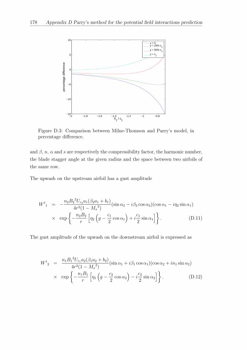
178 Appendix D Parry’s method for the potential field interactions prediction
−2 −1.8 −1.6 −1.4 −1.2 −1 −0.8−15
−10
−5
0
5
10
X2 / c
2
perc
enta
ge d
iffer
ence
y = 0y = 25% c
2
y = 50% c2
y = c2
Figure D.3: Comparison between Milne-Thomson and Parry’s model, inpercentage difference.
and β, n, α and s are respectively the compressibility factor, the harmonic number,
the blade stagger angle at the given radius and the space between two airfoils of
the same row.
The upwash on the upstream airfoil has a gust amplitude
W t1 = −n2B2
2Ur2a1(β2a1 + b1)
4r2(1−Mx2)
(sinα2 − iβ2 cosα2)(cosα1 − iη2 sinα1)
× exp
−n2B2
r
[η2
(g − c1
2cosα1
)+ i
c1
2sinα1
]. (D.11)
The gust amplitude of the upwash on the downstream airfoil is expressed as
W t2 =
n1B12Ur1a2(β1a2 + b2)
4r2(1−Mx2)
(sinα1 + iβ1 cosα1)(cosα2 + in1 sinα2)
× exp
−n1B1
r
[η1
(g − c2
2cosα2
)− ic2
2sinα2
]. (D.12)
Appendix D Parry’s method for the potential field interactions prediction 179
D.2 Potential due to blade circulation
Parry modeled each airfoil by a point vortex of circulation Γ and expressed the
velocity potential as
φl =iΓ
4πβ
+∞∑n=−∞
1
nExEy, (D.13)
where Ex and Ey are defined in equations (D.10) and (D.10). In the coordinate
system defined in section 6.2, the upwash on the upstream airfoil has a gust am-
plitude
W l1 = −ΓB2
4πr(cosα1 − iη2 sinα1) exp
−Ky2
[η2
(g − c1
2cosα1
)+ i
c1
2sinα1
].
(D.14)
In the coordinate system defined in section 6.3, Parry defines the upwash on the
downstream airfoil with the following gust amplitude
W l2 =
ΓB1
4πr(cosα2 + iη1 sinα2) exp
−Ky1
[η1
(g − c2
2cosα2
)− ic2
2sinα2
].
(D.15)
D.3 Simplification of the distributed source model
for an ellipse
In section 6.2.1, the velocity potential due to blade thickness around an isolated
airfoil (which is modelled as a distribution of point sources) is given by equations
(6.91) and (6.15) and is stated below.
φt =Urtmax
2πβ
c2∫
−c2
∂G∂X
∣∣∣X=Xs
log
(1
β
√(X −Xs)2 + β2Y 2
)dXs (D.16)
Integrating by parts leads to
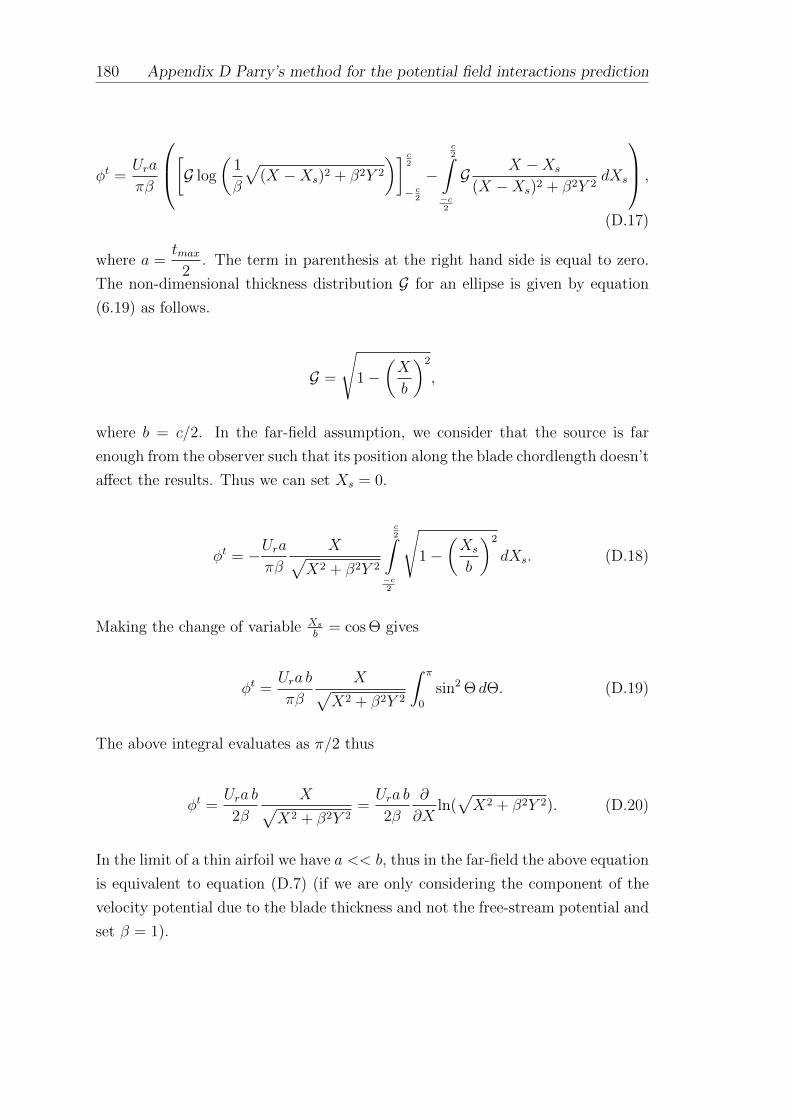
180 Appendix D Parry’s method for the potential field interactions prediction
φt =Ura
πβ
[G log
(1
β
√(X −Xs)2 + β2Y 2
)] c2
− c2
−
c2∫
−c2
G X −Xs
(X −Xs)2 + β2Y 2dXs
,
(D.17)
where a =tmax
2. The term in parenthesis at the right hand side is equal to zero.
The non-dimensional thickness distribution G for an ellipse is given by equation
(6.19) as follows.
G =
√1−
(X
b
)2
,
where b = c/2. In the far-field assumption, we consider that the source is far
enough from the observer such that its position along the blade chordlength doesn’t
affect the results. Thus we can set Xs = 0.
φt = −Uraπβ
X√X2 + β2Y 2
c2∫
−c2
√1−
(Xs
b
)2
dXs. (D.18)
Making the change of variable Xsb
= cos Θ gives
φt =Ura b
πβ
X√X2 + β2Y 2
∫ π
0
sin2 Θ dΘ. (D.19)
The above integral evaluates as π/2 thus
φt =Ura b
2β
X√X2 + β2Y 2
=Ura b
2β
∂
∂Xln(√X2 + β2Y 2). (D.20)
In the limit of a thin airfoil we have a << b, thus in the far-field the above equation
is equivalent to equation (D.7) (if we are only considering the component of the
velocity potential due to the blade thickness and not the free-stream potential and
set β = 1).
References
Abramowitz, M. and Stegun, I. A. (1964). Handbook of mathematical functions:
with formulas, graphs, and mathematical tables, volume 55. Courier Corpora-
tion.
Adamczyk, J. (1971). Passage of an isolated airfoil through a three-dimensional
disturbance. PhD thesis, Ph. D. Thesis, Dept. of Mechanical Engineering. Uni-
versity of Connecticut.
Airbus (2013). Global market forecast: Future journeys 2013-2032. Technical re-
port, Airbus, 2013. URL http://www. airbus. com/company/market/forecast/.
Amiet, R. (1986). Diffraction of sound by a half-plane in a uniform flow. UTRC
Report, 86:17.
Amiet, R. (1991). Unified aeroacoustics analysis for high speed turboprop aero-
dynamics and noise. vol. ii - development of theory for wing shielding. NASA
CR 185192.
Amiet, R. K., Egolf, C., and Simonich, J. C. (1989). Noise produced by turbulent
flow into a rotor: Theory manual for noise calculation.
Ashley, H. and Landahl, M. (1965). Aerodynamics of wings and bodies. Courier
Corporation.
Blandeau, V. (2011). Aerodynamic broadband noise from contra-rotating open
rotors. PhD thesis, University of Southampton.
Blandeau, V. P., Joseph, P. F., Jenkins, G., and Powles, C. J. (2011). Comparison
of sound power radiation from isolated airfoils and cascades in a turbulent flow.
The Journal of the Acoustical Society of America, 129(6):3521–3530.
Block, P. (1986). Experimental study of the effects of installation on singleand
counter-rotation propeller noise. Unknown, 1.
181

182 REFERENCES
Brandvik, T., Hall, C., and Parry, A. B. (2012). Angle-of-attack effects on counter-
rotating propellers at take-off. In ASME Turbo Expo 2012: Turbine Technical
Conference and Exposition, pages 523–534. American Society of Mechanical En-
gineers.
Brandvik, T. and Pullan, G. (2011). An accelerated 3d navier–stokes solver for
flows in turbomachines. Journal of turbomachinery, 133(2):021025.
Brookfield, J., Waitz, I., and Sell, J. (1997). Wake decay: Effect of freestream
swirl. In ASME 1997 International Gas Turbine and Aeroengine Congress and
Exhibition, pages V001T03A097–V001T03A097. American Society of Mechani-
cal Engineers.
Brouwer, H. (2016). The scattering of open rotor tones by a cylindrical fuselage
and its boundary layer. In 22nd AIAA/CEAS Aeroacoustics Conference, page
2741.
Carazo, A., Roger, M., and Omais, M. (2011). Analytical prediction of wake-
interaction noise in counter-rotation open rotors. In 17th AIAA/CEAS Aeroa-
coustics Conference.
Carley, M. (1996). Time domain calculation of noise generated by a propeller in a
flow. PhD thesis, University of Dublin.
Clair, V. and Gabard, G. (2015). Numerical assessment of the scattering of acoustic
waves by turbulent structures. In 21st AIAA/CEAS Aeroacoustics Conference,
page 2680.
Denton, J. (1983). An improved time-marching method for turbomachinery flow
calculation. Journal of engineering for power, 105(3):514–521.
Ekoule, C., McAlpine, A., Kingan, M., Sohoni, N., and Parry, A. (2015). Use of
a hybrid cfd/analytical method for the prediction of advanced open rotor tone
noise. In 21st AIAA/CEAS Aeroacoustics Conference, page 2357.
Envia, E. (1991). Prediction of noise field of a propfan at angle of attack.
Ewert, R., Kornow, O., Tester, B., Powles, C., Delfs, J., and Rose, M. (2008).
Spectral broadening of jet engine turbine tones. AIAA Paper, 2940:2008.
Farassat, F. (1981). Linear acoustic formulas for calculation of rotating blade
noise. AIAA journal, 19(9):1122–1130.

REFERENCES 183
Farassat, F. (1986). Prediction of advanced propeller noise in the time domain.
AIAA journal, 24(4):578–584.
Farassat, F. and Brentner, K. S. (1998). The acoustic analogy and the prediction
of the noise of rotating blades. Theoretical and Computational Fluid Dynamics,
10(1-4):155–170.
Fuller, C. (1989). Free-field correction factor for spherical acoustic waves impinging
on cylinders. AIAA journal, 27(12):1722–1726.
Garrick, I. and Watkins, C. E. (1954). A theoretical study of the effect of forward
speed on the free-space sound-pressure fleld around propellers.
Goldstein, M. (1974). Unified approach to aerodynamic sound generation in the
presence of solid boundaries. The Journal of the Acoustical Society of America,
56(2):497–509.
Gutin, L. (1936). On the sound field of a rotating propeller. Zhurnal tekhnicheskoi
fiziki, 6:899–909.
Hanson, D. (1984). Shielding of prof-fan cabin noise by the fuselage boundary
layer. Journal of Sound and Vibration, 92(4):591–598.
Hanson, D. (1995). Sound from a propeller at angle of attack: a new theoretical
viewpoint. Proceedings of the Royal Society of London. Series A: Mathematical
and Physical Sciences, 449(1936):315–328.
Hanson, D. and Magliozzi, B. (1985). Propagation of propeller tone noise through
a fuselage boundary layer. Journal of Aircraft, 22(1):63–70.
Hanson, D. B. (1985a). Near-field frequency-domain theory for propeller noise.
AIAA journal, 23(4):499–504.
Hanson, D. B. (1985b). Noise of counter-rotation propellers. Journal of Aircraft,
22(7):609–617.
Hanson, D. B. and Parzych, D. J. (1993). Theory for noise of propellers in angular
inflow with parametric studies and experimental verification.
Hanson, D. J. K. (1980). Helicoidal surface theory for harmonic noise of propellers
in the far field. AIAA Journal, 18(10):1213–1220.
Hubbard, H. H. (1948). Sound from dual-rotating and multiple single-rotating
propellers. National Advisory Committee for Aeronautics.

184 REFERENCES
Hubbard, H. H. and Regier, A. A. (1950). Free-space oscillating pressures near
the tips of rotating propellers. NACA.
Izzo, D. (2005). Application of a dirac delta disintegration technique to the statis-
tics of orbiting objects. In 4th European Conference on Space Debris, volume
587, page 673.
Jaouani, N., Roger, M., Node-Langlois, T., and Serre, G. (2015). Analytical
prediction of the pylon-wake effect on the tonal noise radiated by the front rotor
of cror propulsion systems. In 21st AIAA/CEAS Aeroacoustics Conference, page
2985.
Jaouani, N., Roger, M., Node-Langlois, T., and Serre, G. (2016). Effect of a model
leading-edge vortex on the blade aerodynamic response for application to cror
tonal noise predictions. In 22nd AIAA/CEAS Aeroacoustics Conference, page
2744.
Jaron, R., Moreau, A., and Guerin, S. (2014). Rans-informed fan noise prediction:
separation and extrapolation of rotor wake and potential field. AIAA Paper,
(2014-2946).
Kemp, N. and Sears, W. (1953). Aerodynamic interference between moving blade
rows. Journal of the Aeronautical Sciences, 22(9):585.
Kingan, M. and Sureshkumar, P. (2014). Open rotor centrebody scattering. Jour-
nal of Sound and Vibration, 333(2):418–433.
Kingan, M. J., Ekoule, C. M., Parry, A. B., and Britchford, K. M. (2014). Analysis
of advanced open rotor noise measurements. In 20th AIAA/CEAS Aeroacoustics
Conference. AIAA Aviation.
Kingan, M. J., Powles, C., and Self, R. H. (2010). Effect of centerbody scattering
on advanced open-rotor noise. AIAA journal, 48(5):975–980.
Kingan, M. J. and Self, R. H. (2009). Counter-rotation propeller tip vortex inter-
action noise. In 15th AIAA/CEAS Aeroacoustics conference, Miami, Florida,
page 3135.
Kingan, M. J. and Self, R. H. (2012). Open rotor tone scattering. Journal of
Sound and Vibration, 331(8):1806–1828.
Krejsa, E. A. (1990). Prediction of the noise from a propeller at angle of attack.
National Aeronautics and Space Administration.
REFERENCES 185
Landahl, M. T. (1989). Unsteady transonic flow. CUP Archive.
Lowson, M. (1965). The sound field for singularities in motion. Proceedings of
the Royal Society of London. Series A. Mathematical and Physical Sciences,
286(1407):559–572.
Lu, H. (1990). Fuselage boundary-layer effects on sound propagation and scatter-
ing. AIAA journal, 28(7):1180–1186.
Magliozzi, B. and Hanson, D. (1991). 1 propeller and propfan noise. Thery nd
racic, page 1.
Majjigi, R., Uenishi, K., and Gliebe, P. R. (1989). An investigation of counterro-
tating tip vortex interaction. Unknown, 1.
Mani, R. (1990). The radiation of sound from a propeller at angle of attack.
Proceedings of the Royal Society of London. Series A: Mathematical and Physical
Sciences, 431(1882):203–218.
McAlpine, A. and Kingan, M. J. (2012). Far-field sound radiation due to an
installed open rotor. International Journal of Aeroacoustics, 11(2):213–246.
McAlpine, A., Powles, C., and Tester, B. (2013). A weak-scattering model for
turbine-tone haystacking. Journal of Sound and Vibration, 332(16):3806–3831.
Milne-Thomson, L. M. (1968). Theoretical hydrodynamics. Courier Corporation.
Paquet, C., Julliard, E., Genoulaz, N., Ricouard, J., and Spiegel, P. (2014). Z08:
low-speed aero-acoustic experimental characterization of open rotor installation
on aircraft. In 20th AIAA/CEAS Aeroacoustics Conference. AIAA Aviation.
Parry, A., Kingan, M., and Tester, B. (2011). Relative importance of open rotor
tone and broadband noise sources. In 17th AIAA/CEAS Aeroacoustics Confer-
ence, Portland, Oregon, pages 5–8.
Parry, A. B. (1988). Theoretical prediction of counter-rotating propeller noise.
PhD thesis, University of Leeds.
Peake, N. and Parry, A. B. (2012). Modern challenges facing turbomachinery
aeroacoustics. Annual Review of Fluid Mechanics, 44:227–248.
Powles, C. J., Tester, B. J., and McAlpine, A. (2010). A weak-scattering model
for turbine-tone haystacking outside the cone of silence. International Journal
of Aeroacoustics, 10(1):17–50.

186 REFERENCES
Reynolds, B. (1979). Characteristics of the wake of a lightly loaded compressor or
fan rotor.
Ricouard, J., Julliard, E., Omais, M., Regnier, V., Parry, A., and Baralon,
S. (2010). Installation effects on contra-rotating open rotor noise. In 16th
AIAA/CEAS Aeroacoustics Conference. SAS, AIRBUS OPERATIONS, AIAA
Aviation.
Roger, M., Schram, C., and Moreau, S. (2012). On open rotor blade-vortex inter-
action noise. In 18th AIAA/CEAS Aeroacoustics conference, Colorado Springs,
CO.
Santana, L. D., Schram, C., and Desmet, W. (2013). An experimental procedure
for the determination of wake-airfoil interaction noise parameters. In Proceedings
of the 19th AIAA/CEAS Aeroacoustics Conference, AIAA 2013, volume 2060,
pages 27–29.
Shivashankara, B., Johnson, D., and Cuthbertson, R. (1990). Installation effects
on counter rotating propeller noise. In AIAA, Space Programs and Technologies
Conference, volume 1.
Sinnige, T., Lynch, K. P., Ragni, D., Eitelberg, G., and Veldhuis, L. L. (2015).
Aerodynamic and aeroacoustic effects of pylon trailing edge blowing on pusher
propeller installation. In 21st AIAA/CEAS Aeroacoustics Conference, page
2356.
Sohoni, N., Hall, C., Brandvik, T., and Parry, A. (2015). Prediction and mea-
surement of unsteady blade surface pressures on an open rotor. In ASME Turbo
Expo 2015: Turbine Technical Conference and Exposition, pages V001T01A007–
V001T01A007. American Society of Mechanical Engineers.
Stuff, R. (1988). Noise field of a propeller with angular inflow. AIAA journal,
26(7):777–782.
Tanna, H., URRIN, R., and LUMBLEE, H. (1981). Installation effects on propeller
noise. Journal of Aircraft, 18(4):303–309.
Vion, L. (2013). Modifications des tourbillons d’extremite d’helices contra-rotatives
en vue d’une reduction des nuisances sonores. PhD thesis, Ecole Polytechnique
X.

REFERENCES 187
Watkins, C. E. and Durling, B. J. (1956). A Method for Calculation of Free-
space Sound Pressures Near a Propeller in Flight Including Considerations of
the Chordwise Blade Loading. National Advisory Committee for Aeronautics.
Woodward, R. P. (1987). Noise of a model high speed counterrotation propeller
at simulated takeoff/approach conditions (f7/a7).