Advanced Term Structure

Carnegie Mellon UniversityCarnegie Mellon University

Fall 2004Fall 2004

Structure of the course

First 2 weeks: Term structure theoryFirst 2 weeks: Term structure theory Use Professor Shreve’s notes, Chapter 10Use Professor Shreve’s notes, Chapter 10

Remaining 5 weeks: Term structure practiceRemaining 5 weeks: Term structure practice No text; just readings and lecture notesNo text; just readings and lecture notes At the beginning we’ll refer to last At the beginning we’ll refer to last

semester’s textsemester’s text Students (in groups of size 1 or 2) will Students (in groups of size 1 or 2) will

implement HJM modelsimplement HJM models

Grades

There will be regular homework There will be regular homework assignments.assignments.

There will be a final examination.There will be a final examination. The homework assignments (together) will The homework assignments (together) will

count about as much as the final.count about as much as the final.

Miscellaneous items:

I plan to give lectures in NYC on I plan to give lectures in NYC on September 13 and on October 25September 13 and on October 25

We need to agree on meeting times with the We need to agree on meeting times with the TA (Sean).TA (Sean).

Recall some fundamental ideas:

In a market with one or more securities In a market with one or more securities trading, we always require the existence of trading, we always require the existence of an equivalent martingale measure (for which an equivalent martingale measure (for which all discounted security prices are all discounted security prices are martingales). We do this to avoid arbitrage.martingales). We do this to avoid arbitrage.

Remember that two measures are Remember that two measures are “equivalent” provided they have the same “equivalent” provided they have the same null sets.null sets.

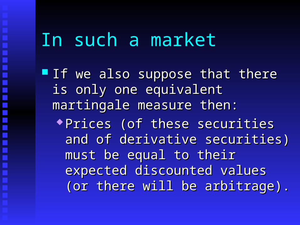
In such a market

If we also suppose that there is only one If we also suppose that there is only one equivalent martingale measure then:equivalent martingale measure then: Prices (of these securities and of Prices (of these securities and of

derivative securities) must be equal to derivative securities) must be equal to their expected discounted values (or there their expected discounted values (or there will be arbitrage).will be arbitrage).

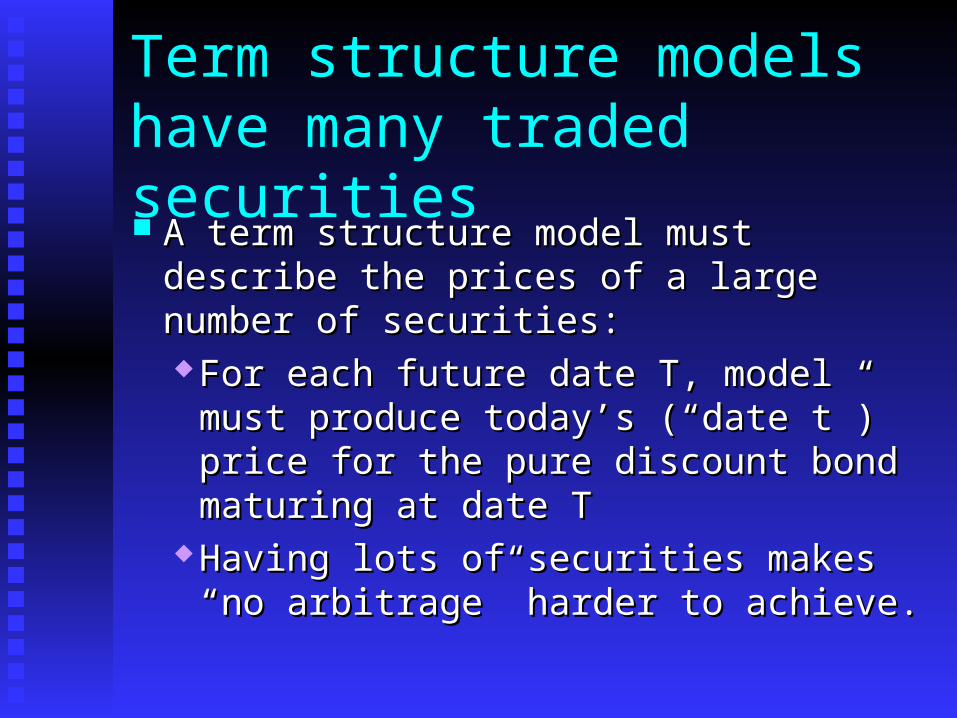
Term structure models have many traded securities A term structure model must describe the A term structure model must describe the

prices of a large number of securities:prices of a large number of securities: For each future date T, model must For each future date T, model must

produce today’s (“date t”) price for the produce today’s (“date t”) price for the pure discount bond maturing at date Tpure discount bond maturing at date T

Having lots of securities makes “no Having lots of securities makes “no arbitrage” harder to achieve.arbitrage” harder to achieve.

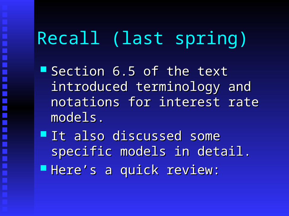
Recall (last spring)

Section 6.5 of the text introduced Section 6.5 of the text introduced terminology and notations for interest rate terminology and notations for interest rate models.models.

It also discussed some specific models in It also discussed some specific models in detail. detail.

Here’s a quick review:Here’s a quick review:

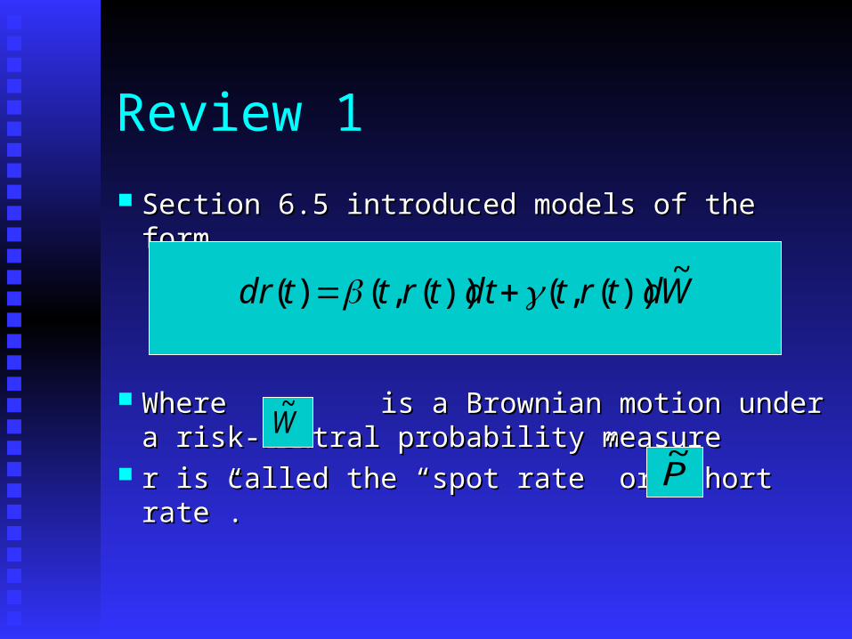
Review 1

Section 6.5 introduced models of the formSection 6.5 introduced models of the form

Where is a Brownian motion under a Where is a Brownian motion under a risk-neutral probability measure risk-neutral probability measure

r is called the “spot rate” or “short rate”.r is called the “spot rate” or “short rate”.

Wdtrtdttrttdr~

))(,())(,()(

W~

P~

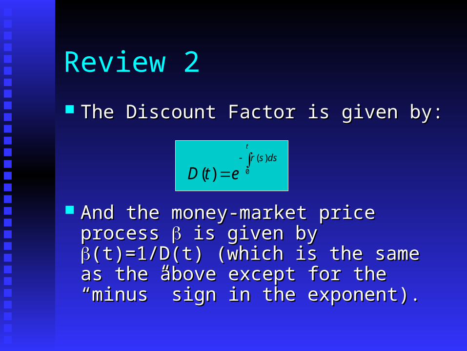
Review 2

The Discount Factor is given by:The Discount Factor is given by:

And the money-market price process And the money-market price process is is given by given by (t)=1/D(t) (which is the same as (t)=1/D(t) (which is the same as the above except for the “minus” sign in the the above except for the “minus” sign in the exponent).exponent).

t

dssr

etD 0

)(

)(

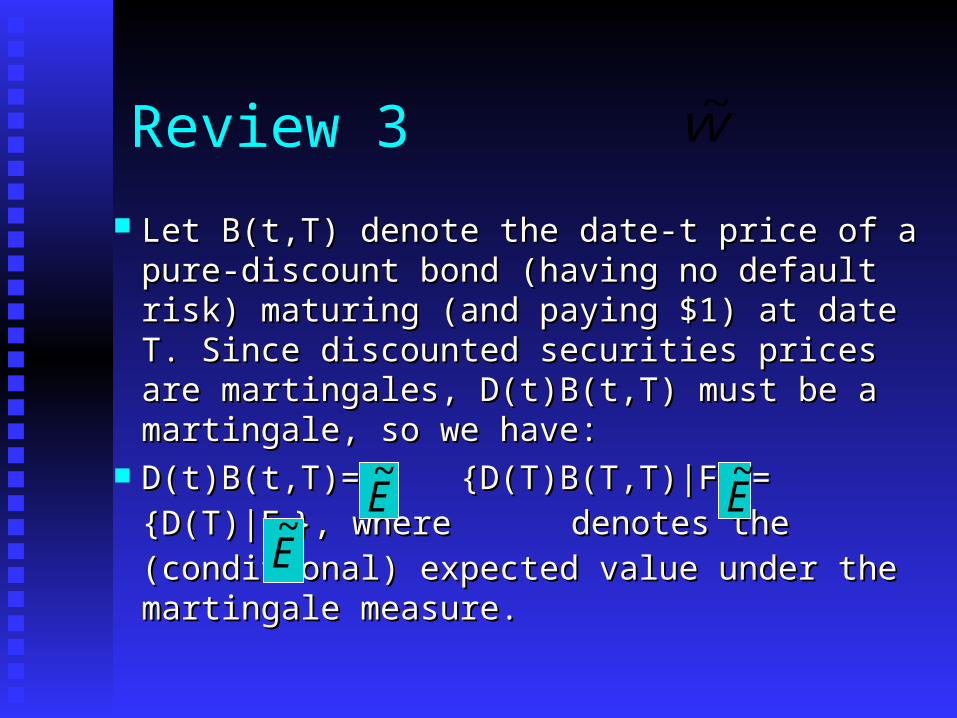
Review 3

Let B(t,T) denote the date-t price of a pure-Let B(t,T) denote the date-t price of a pure-discount bond (having no default risk) discount bond (having no default risk) maturing (and paying $1) at date T. Since maturing (and paying $1) at date T. Since discounted securities prices are martingales, discounted securities prices are martingales, D(t)B(t,T) must be a martingale, so we have:D(t)B(t,T) must be a martingale, so we have:

D(t)B(t,T)= {D(T)B(T,T)|FD(t)B(t,T)= {D(T)B(T,T)|Ftt}= {D(T)|F}= {D(T)|Ftt}, },

where denotes the (conditional) expected where denotes the (conditional) expected value under the martingale measure.value under the martingale measure.

W~

E~

E~

E~

Review 4

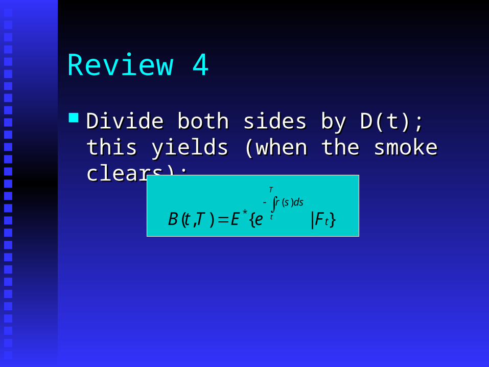
Divide both sides by D(t); this yields (when Divide both sides by D(t); this yields (when the smoke clears):the smoke clears):

}|{),()(

*t

dssr

FeETtB

T

t

Review 5Two choices for Two choices for and and : : dr(t)=(a(t)-b(t)r(t))dt+dr(t)=(a(t)-b(t)r(t))dt+(t) (t)(t) (t)

This is the Hull-White modelThis is the Hull-White model

dr(t)=(a - b r(t))dt+dr(t)=(a - b r(t))dt+(r(t))(r(t))0.5 0.5 (t)(t)This is the Cox-Ingersoll-Ross model.This is the Cox-Ingersoll-Ross model.

Wd~

Wd~

Review 6

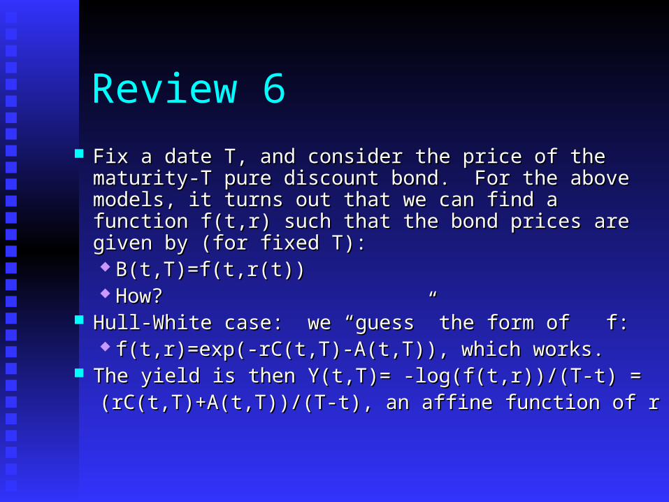
Fix a date T, and consider the price of the maturity-T Fix a date T, and consider the price of the maturity-T pure discount bond. For the above models, it turns out pure discount bond. For the above models, it turns out that we can find a function f(t,r) such that the bond prices that we can find a function f(t,r) such that the bond prices are given by (for fixed T):are given by (for fixed T): B(t,T)=f(t,r(t))B(t,T)=f(t,r(t)) How?How?

Hull-White case: we “guess” the form of f:Hull-White case: we “guess” the form of f: f(t,r)=exp(-rC(t,T)-A(t,T)), which works.f(t,r)=exp(-rC(t,T)-A(t,T)), which works.

The yield is then Y(t,T)= -log(f(t,r))/(T-t) =The yield is then Y(t,T)= -log(f(t,r))/(T-t) =(rC(t,T)+A(t,T))/(T-t), an affine function of r(rC(t,T)+A(t,T))/(T-t), an affine function of r

Review 7

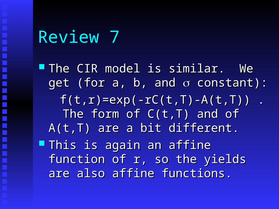
The CIR model is similar. We get (for a, b, The CIR model is similar. We get (for a, b, and and constant): constant):

f(t,r)=exp(-rC(t,T)-A(t,T)) . The form of f(t,r)=exp(-rC(t,T)-A(t,T)) . The form of C(t,T) and of A(t,T) are a bit different.C(t,T) and of A(t,T) are a bit different.

This is again an affine function of r, so the This is again an affine function of r, so the yields are also affine functions.yields are also affine functions.

Limitations of these models

Models generated by specifying the Models generated by specifying the behavior of the “spot rate” or “short rate,” behavior of the “spot rate” or “short rate,” are called “spot-rate” or “short-rate” are called “spot-rate” or “short-rate” models.models.

These two are both “one-factor” models. These two are both “one-factor” models. We’ll see later that these models do not We’ll see later that these models do not capture the “correlations” in the motion of capture the “correlations” in the motion of the yield curve.the yield curve.

“Calibration”

Recall that in general we need the martingale Recall that in general we need the martingale measure P* to be equivalent to the “true” measure P. measure P* to be equivalent to the “true” measure P. What does this mean? What does this mean? The arguments in chapter 4 of the text (in The arguments in chapter 4 of the text (in

particular equation 4.8.3) can be extended to particular equation 4.8.3) can be extended to show that the quadratic variation of a stochastic show that the quadratic variation of a stochastic integral can be computed exactly (for a given integral can be computed exactly (for a given sample path) by breaking the interval into small sample path) by breaking the interval into small pieces, squaring the change in the process over pieces, squaring the change in the process over each piece, adding these up, and taking the limit each piece, adding these up, and taking the limit as the intervals get smaller.as the intervals get smaller.

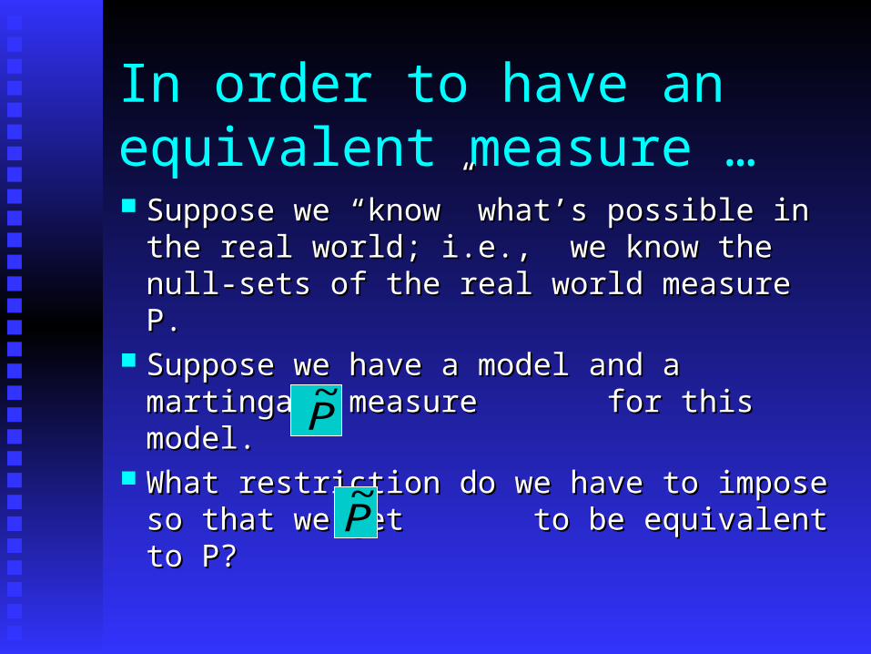
In order to have an equivalent measure … Suppose we “know” what’s possible in the Suppose we “know” what’s possible in the

real world; i.e., we know the null-sets of real world; i.e., we know the null-sets of the real world measure P.the real world measure P.

Suppose we have a model and a martingale Suppose we have a model and a martingale measure for this model.measure for this model.

What restriction do we have to impose so What restriction do we have to impose so that we get to be equivalent to P?that we get to be equivalent to P?

P~

P~

A necessary condition:

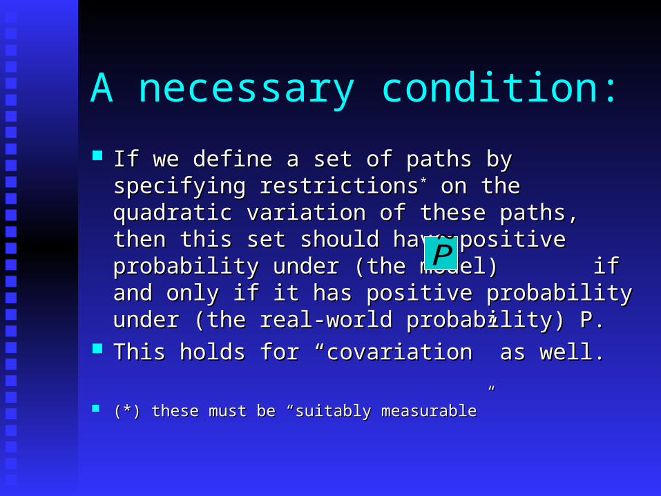
If we define a set of paths by specifying If we define a set of paths by specifying restrictionsrestrictions** on the quadratic variation of these on the quadratic variation of these paths, then this set should have positive paths, then this set should have positive probability under (the model) if and only if it probability under (the model) if and only if it has positive probability under (the real-world has positive probability under (the real-world probability) P.probability) P.

This holds for “covariation” as well.This holds for “covariation” as well.

(*) these must be “suitably measurable”(*) these must be “suitably measurable”

P~

An example For the Hull-White model we haveFor the Hull-White model we have

Hence the quadratic variation isHence the quadratic variation is

For each t>0 the left side is a random variable, but For each t>0 the left side is a random variable, but the right side is a number. Hence (under the the right side is a number. Hence (under the model), for each t we know that [r,r](t) is, with model), for each t we know that [r,r](t) is, with probability 1, equal to that number. probability 1, equal to that number.

t t

sWdsdssrsbsartr0 0

)(~

)())()()((()0()(

t

dsstrr0

2 )()](,[

This we can check! You can compute (in principle, and very nearly in You can compute (in principle, and very nearly in

practice) the quadratic variation of an observed practice) the quadratic variation of an observed sample path. And by the observation on the sample path. And by the observation on the previous slide, it should be equal to the integal on previous slide, it should be equal to the integal on the right-hand side. the right-hand side.

Now an optimistic view is that the observed Now an optimistic view is that the observed quadratic variation tells you the function quadratic variation tells you the function (.). But (.). But what it really tells you is the function what it really tells you is the function (.) in the (.) in the past, and we usually need to know it in the future. past, and we usually need to know it in the future.

Recall: If an event occurs with probability 1, it Recall: If an event occurs with probability 1, it should occur EVERY time you run the experimentshould occur EVERY time you run the experiment

And a stronger result for the CIR model:

dR(t)=(a-bR(t))dt+dR(t)=(a-bR(t))dt+(R(t))(R(t))0.5 0.5 dWdW**(t), so(t), so

We re-write this asWe re-write this as

t

dssrtrr0

2)()](,[

2

0

)(

)](,[

t

dssr

trr

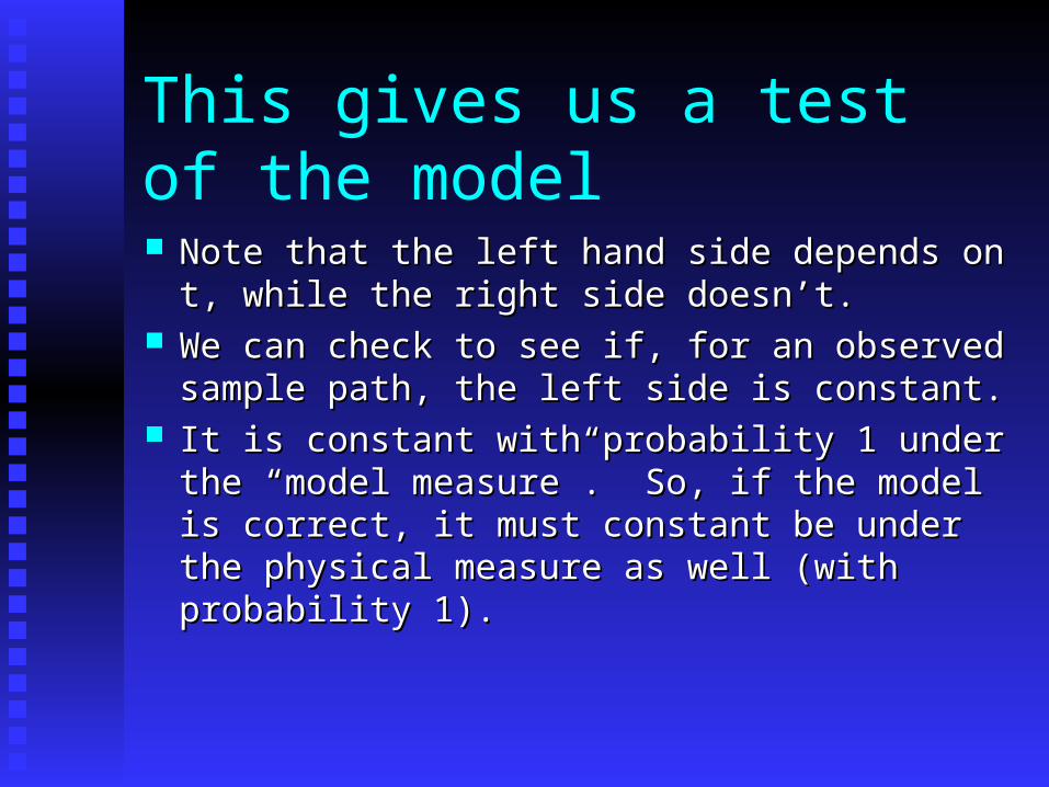
This gives us a test of the model

Note that the left hand side depends on t, while the Note that the left hand side depends on t, while the right side doesn’t.right side doesn’t.

We can check to see if, for an observed sample We can check to see if, for an observed sample path, the left side is constant.path, the left side is constant.

It is constant with probability 1 under the “model It is constant with probability 1 under the “model measure”. So, if the model is correct, it must measure”. So, if the model is correct, it must constant be under the physical measure as well constant be under the physical measure as well (with probability 1).(with probability 1).

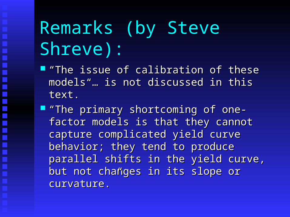
Remarks (by Steve Shreve):

““The issue of calibration of these models … The issue of calibration of these models … is not discussed in this text.”is not discussed in this text.”

““The primary shortcoming of one-factor The primary shortcoming of one-factor models is that they cannot capture models is that they cannot capture complicated yield curve behavior; they tend complicated yield curve behavior; they tend to produce parallel shifts in the yield curve, to produce parallel shifts in the yield curve, but not changes in its slope or curvature.”but not changes in its slope or curvature.”

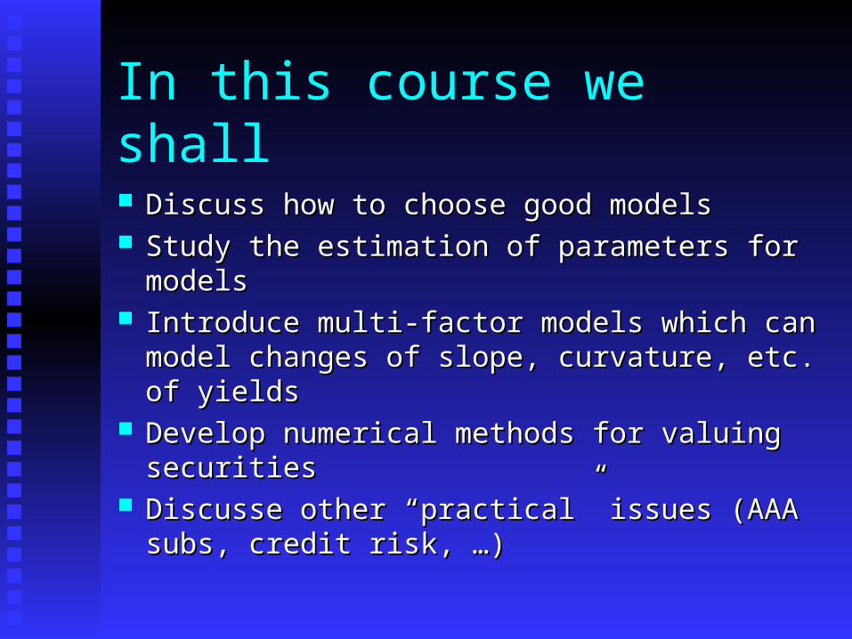
In this course we shall

Discuss how to choose good modelsDiscuss how to choose good models Study the estimation of parameters for modelsStudy the estimation of parameters for models Introduce multi-factor models which can model Introduce multi-factor models which can model

changes of slope, curvature, etc. of yields changes of slope, curvature, etc. of yields Develop numerical methods for valuing securitiesDevelop numerical methods for valuing securities Discusse other “practical” issues (AAA subs, Discusse other “practical” issues (AAA subs,

credit risk, …)credit risk, …)

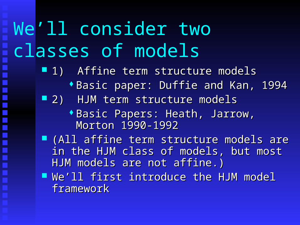
We’ll consider two classes of models

1) Affine term structure models1) Affine term structure modelsBasic paper: Duffie and Kan, 1994Basic paper: Duffie and Kan, 1994

2) HJM term structure models2) HJM term structure modelsBasic Papers: Heath, Jarrow, Morton 1990-Basic Papers: Heath, Jarrow, Morton 1990-

19921992 (All affine term structure models are in the HJM (All affine term structure models are in the HJM

class of models, but most HJM models are not class of models, but most HJM models are not affine.)affine.)

We’ll first introduce the HJM model frameworkWe’ll first introduce the HJM model framework

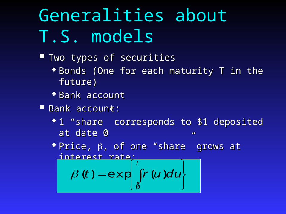
Generalities about T.S. models

Two types of securitiesTwo types of securities Bonds (One for each maturity T in the future)Bonds (One for each maturity T in the future) Bank accountBank account

Bank account:Bank account: 1 “share” corresponds to $1 deposited at date 01 “share” corresponds to $1 deposited at date 0 Price, Price, , of one “share” grows at interest rate:, of one “share” grows at interest rate:

t

duurt0

)(exp)(

Bond prices B(t,T)Bond prices B(t,T) B(t,T) = price at date t of default-risk-free pure-B(t,T) = price at date t of default-risk-free pure-

discount-bond paying $1 at Tdiscount-bond paying $1 at T We always have B(T,T)=1We always have B(T,T)=1 Prices will always be semi-martingales; for Prices will always be semi-martingales; for

one-factor models driven by Brownian motion one-factor models driven by Brownian motion we havewe have

Note: The values of Note: The values of and and can depend on can depend on “other information” known at time t.“other information” known at time t.

No arbitrage: we want B(t,T)/No arbitrage: we want B(t,T)/(t) to be a (t) to be a martingale for each T.martingale for each T.

)(),(),(),(),(),( tdWTtBTtdtTtBTtTtBdt

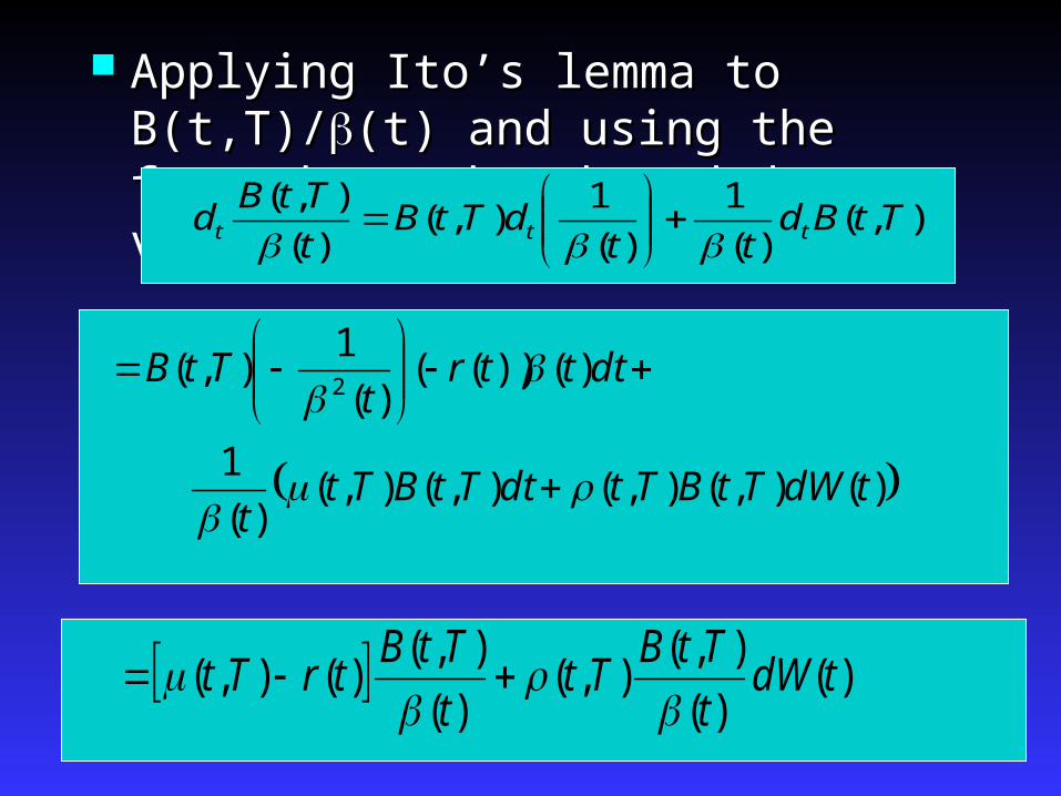
Applying Ito’s lemma to B(t,T)/Applying Ito’s lemma to B(t,T)/(t) and (t) and using the fact that using the fact that has bounded variation: has bounded variation:

),()(

1

)(

1),(

)(

),(TtBd

ttdTtB

t

TtBd ttt

)(),(),(),(),()(

1

)())(()(

1),(

2

tdWTtBTtdtTtBTtt

dtttrt

TtB

)()(

),(),(

)(

),()(),( tdW

t

TtBTt

t

TtBtrTt

Under an equivalent martingale measure The coefficient of “dt” would have to be 0The coefficient of “dt” would have to be 0 This means that This means that (t,T)=r(t).(t,T)=r(t). Or, if we wanted to change measures, we’d Or, if we wanted to change measures, we’d

need need

We’d need the We’d need the samesame change of measure to change of measure to work for every T! (strong restriction!)work for every T! (strong restriction!)

e.m.m.an under motion Brownian a

is ~

where)(~

),( toequal be to

)(),()(),(

WtWdTt

tdWTtdttrTt

Prices of bonds

Assume that P is the equivalent mart. meas.Assume that P is the equivalent mart. meas. Thus for each T, is a martingaleThus for each T, is a martingale

Moreover, B(T,T)=1Moreover, B(T,T)=1 HenceHence

So: So:

)(

),(

t

TtB

)(|)(

),(

)(

),(tF

T

TTBE

t

TtB

)(|)(

1)(),( tFTEtTtB

Calibration to initial term structure: Required for term structure models

At date 0 we can observe (in the market) prices for At date 0 we can observe (in the market) prices for pure discount bonds at various maturities.pure discount bonds at various maturities.

A spot-rate model must be “calibrated” to A spot-rate model must be “calibrated” to reproduce this term structure (to avoid arbitrage reproduce this term structure (to avoid arbitrage between “market” and “model”).between “market” and “model”).

It should also be calibrated to the prices of liquid It should also be calibrated to the prices of liquid instruments such as caps, floors and swaptions.instruments such as caps, floors and swaptions.

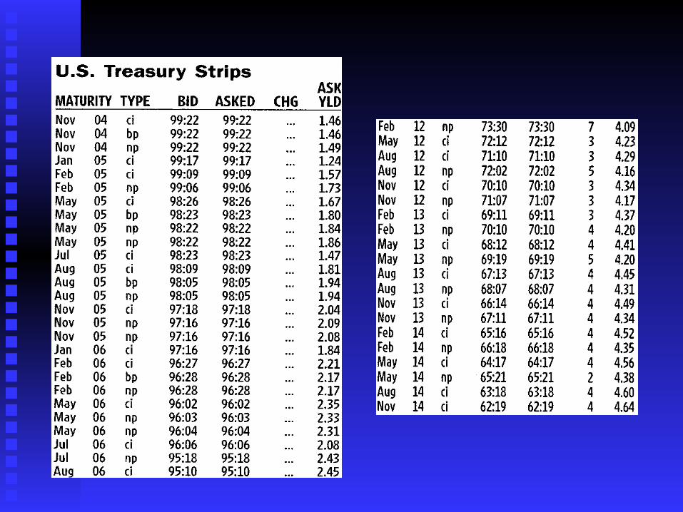
U.S. Treasury instruments

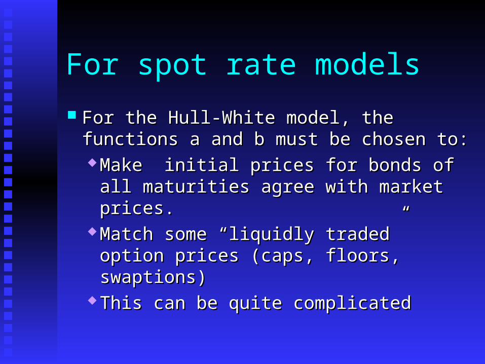
For spot rate models

For the Hull-White model, the functions a For the Hull-White model, the functions a and b must be chosen to:and b must be chosen to: Make initial prices for bonds of all Make initial prices for bonds of all

maturities agree with market prices.maturities agree with market prices. Match some “liquidly traded” option Match some “liquidly traded” option

prices (caps, floors, swaptions)prices (caps, floors, swaptions) This can be quite complicatedThis can be quite complicated

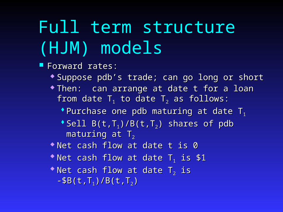
Full term structure (HJM) models

Forward rates:Forward rates: Suppose pdb’s trade; can go long or shortSuppose pdb’s trade; can go long or short Then: can arrange at date t for a loan from date TThen: can arrange at date t for a loan from date T11

to date Tto date T22 as follows: as follows:Purchase one pdb maturing at date TPurchase one pdb maturing at date T11

Sell B(t,TSell B(t,T11)/B(t,T)/B(t,T22) shares of pdb maturing at T) shares of pdb maturing at T22

Net cash flow at date t is 0Net cash flow at date t is 0 Net cash flow at date TNet cash flow at date T11 is $1 is $1 Net cash flow at date TNet cash flow at date T22 is -$B(t,T is -$B(t,T11)/B(t,T)/B(t,T22))

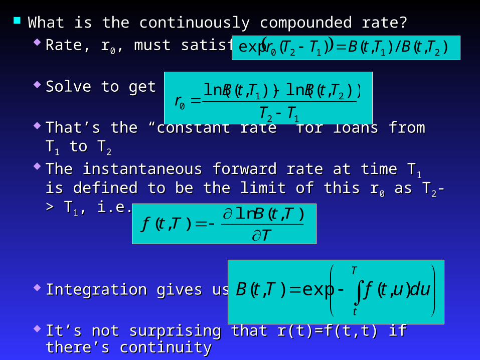
What is the continuously compounded rate?What is the continuously compounded rate? Rate, rRate, r00, must satisfy , must satisfy

Solve to getSolve to get

That’s the “constant rate” for loans from TThat’s the “constant rate” for loans from T11 to T to T22

The instantaneous forward rate at time TThe instantaneous forward rate at time T11 is defined is defined to be the limit of this rto be the limit of this r00 as T as T22-> T-> T11, i.e., i.e.

Integration gives us: Integration gives us:

It’s not surprising that r(t)=f(t,t) if there’s continuityIt’s not surprising that r(t)=f(t,t) if there’s continuity

12

210

)),(ln()),(ln(

TT

TtBTtBr

),(/),()(exp 21120 TtBTtBTTr

T

TtBTtf

),(ln

),(

T

t

duutfTtB ),(exp),(

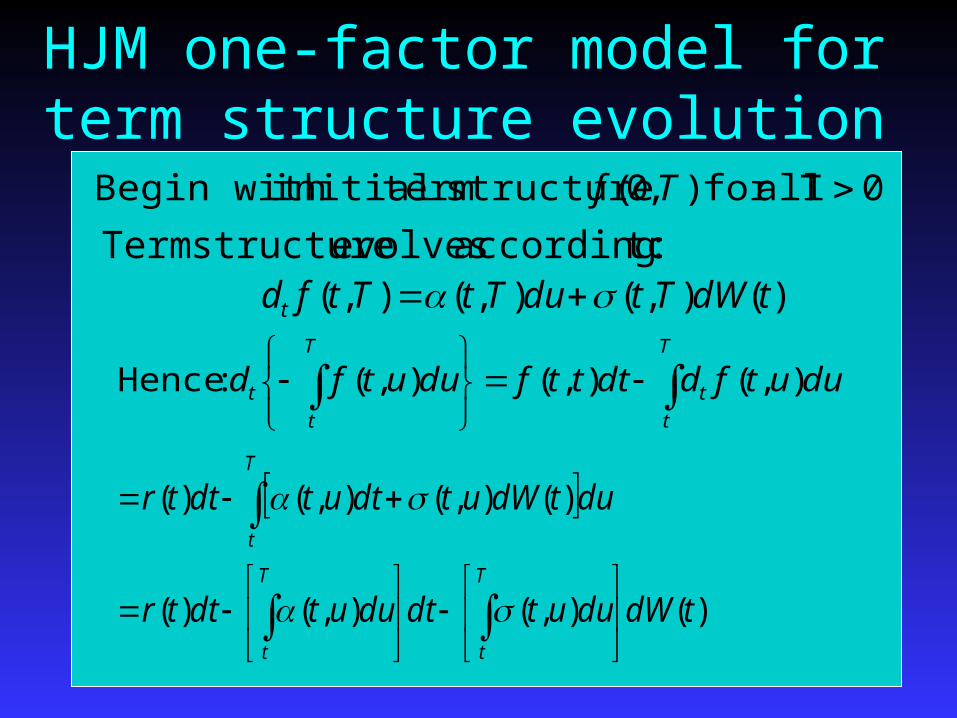
HJM one-factor model for term structure evolution

Hence:Hence:

)(),(),(),( tdWTtduTtTtfdt

T

t

t

T

t

t duutfddtttfduutfd ),(),(),( :Hence

)(),(),()(

)(),(),()(

tdWduutdtduutdttr

dutdWutdtutdttr

T

t

T

t

T

t

0T allfor ),0( structure terminitial Begin with Tf

: toaccording evolves structure Term

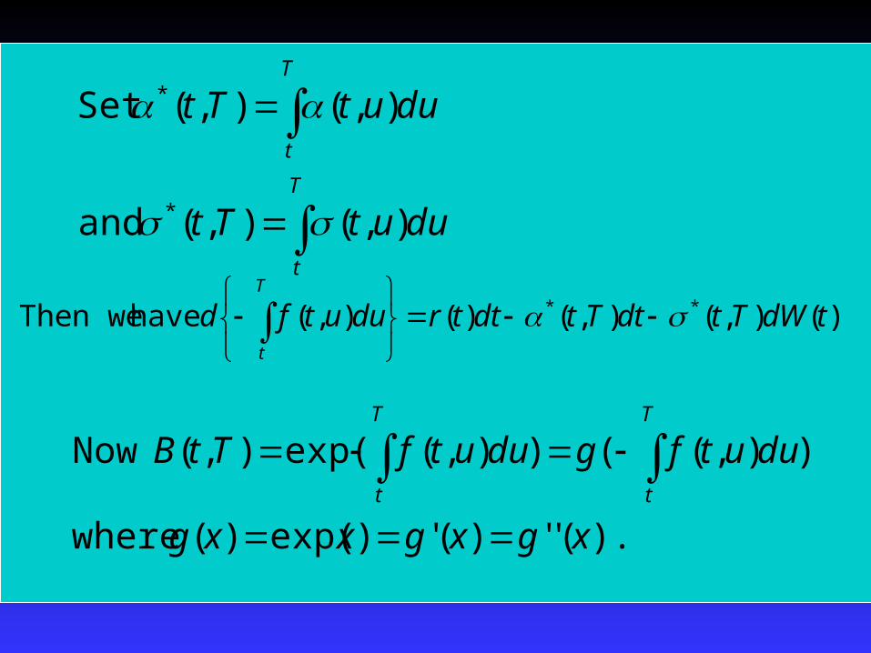
)(),(),()(),( have Then we ** tdWTtdtTtdttrduutfdT

t

T

t

T

t

duutTt

duutTt

),(),( and

),(),(Set

*

*

).('')(')exp()( where

)),(()),(exp(),( Now

xgxgxxg

duutfgduutfTtBT

t

T

t

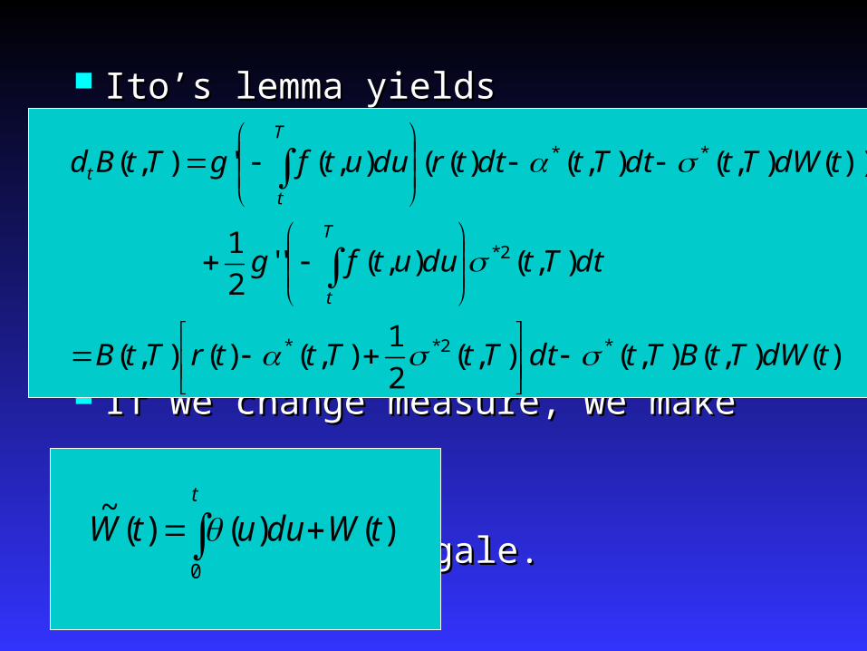
Ito’s lemma yieldsIto’s lemma yields

If we change measure, we make If we change measure, we make

a martingale.a martingale.

)(),(),(),(2

1),()(),(

),(),(''2

1

))(),(),()((),('),(

*2**

2*

**

tdWTtBTtdtTtTttrTtB

dtTtduutfg

tdWTtdtTtdttrduutfgTtBd

T

t

T

t

t

t

tWduutW0

)()()(~

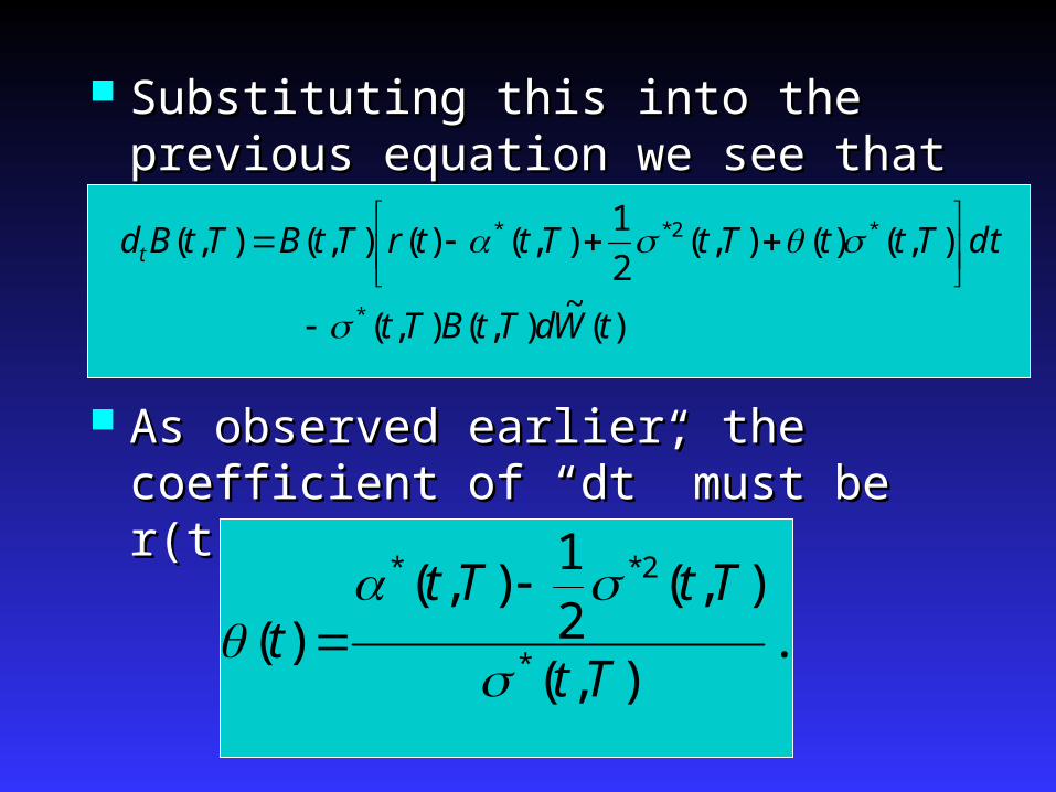
Substituting this into the previous equation Substituting this into the previous equation we see thatwe see that

As observed earlier, the coefficient of “dt” As observed earlier, the coefficient of “dt” must be r(t), so we must havemust be r(t), so we must have

)(~

),(),(

),()(),(2

1),()(),(),(

*

*2**

tWdTtBTt

dtTttTtTttrTtBTtBdt

.),(

),(21

),()(

*

2**

Tt

TtTtt

Remarks on HJM

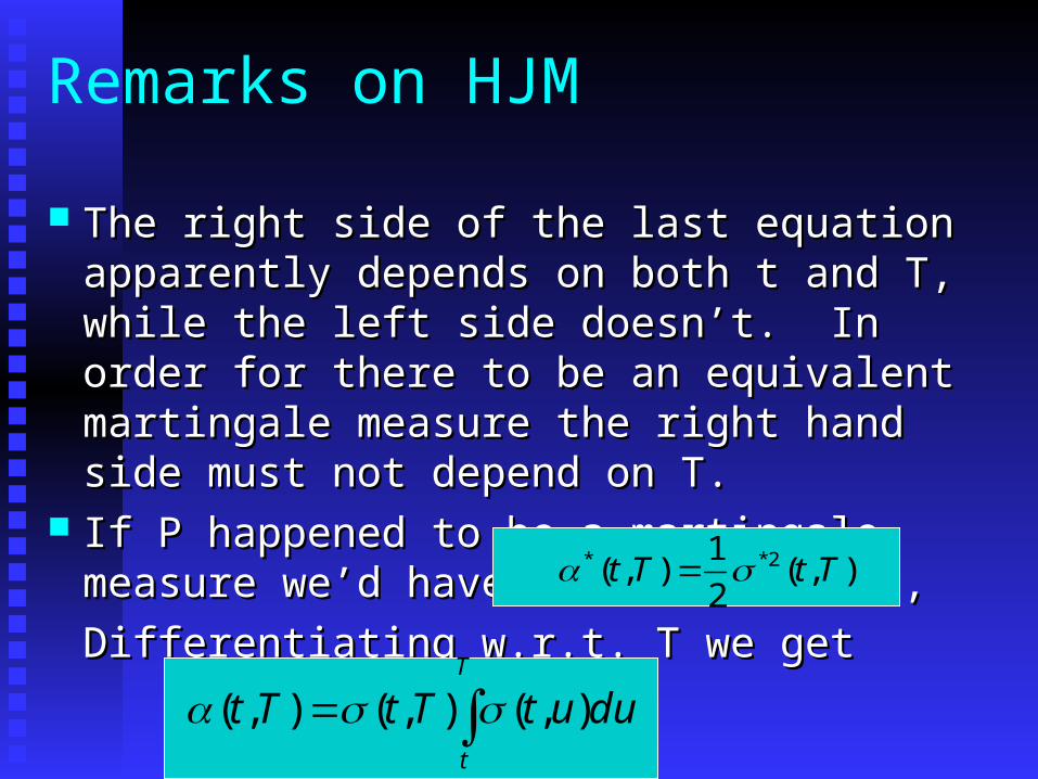
The right side of the last equation apparently The right side of the last equation apparently depends on both t and T, while the left side depends on both t and T, while the left side doesn’t. In order for there to be an equivalent doesn’t. In order for there to be an equivalent martingale measure the right hand side must martingale measure the right hand side must not depend on T.not depend on T.

If P happened to be a martingale measure we’d If P happened to be a martingale measure we’d have found have found =0; i.e.,=0; i.e.,

Differentiating w.r.t. T we getDifferentiating w.r.t. T we get

).,(2

1),( 2** TtTt

T

t

duutTtTt ),(),(),(

Remarks continued

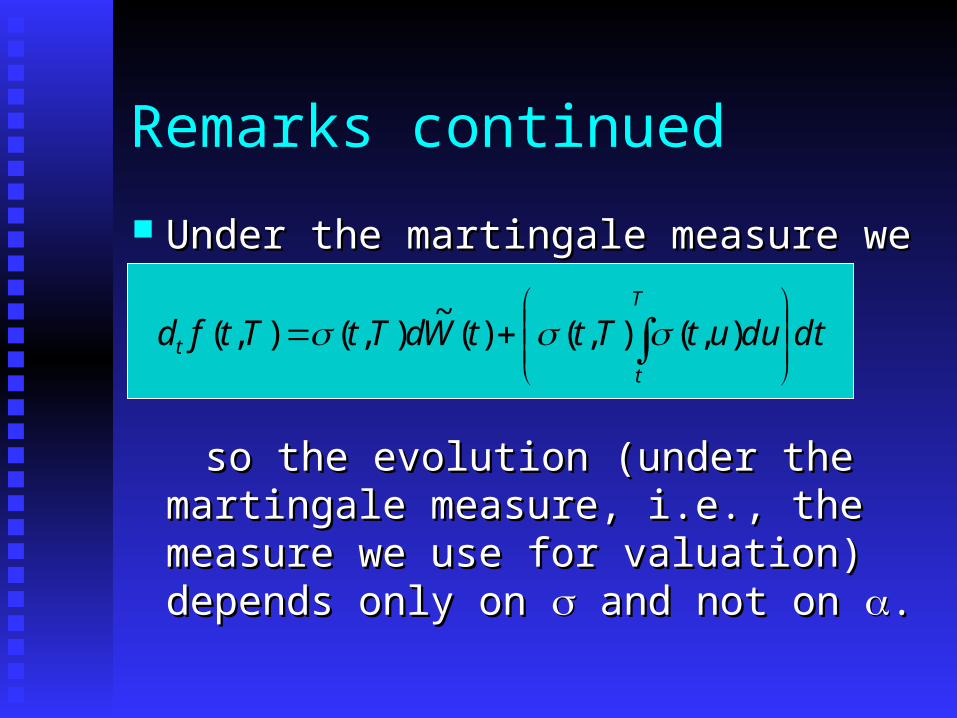
Under the martingale measure we haveUnder the martingale measure we have

so the evolution (under the martingale so the evolution (under the martingale measure, i.e., the measure we use for measure, i.e., the measure we use for valuation) depends only on valuation) depends only on and not on and not on ..

dtduutTttWdTtTtfdT

t

t

),(),()(

~),(),(

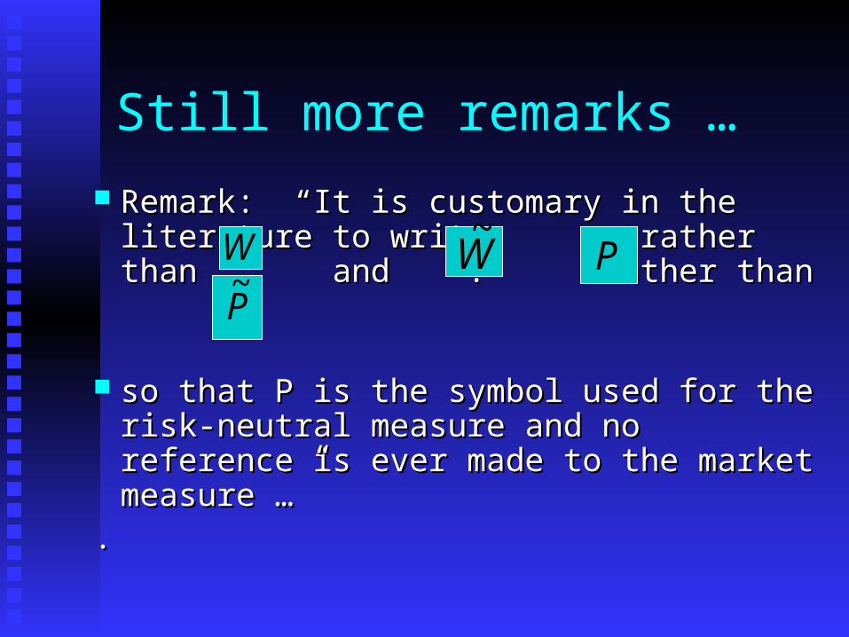
Still more remarks …

Remark: “It is customary in the literature to Remark: “It is customary in the literature to write rather than and . rather write rather than and . rather than than

so that P is the symbol used for the risk-so that P is the symbol used for the risk-neutral measure and no reference is ever neutral measure and no reference is ever made to the market measure …”made to the market measure …”

..

W PP~

W~