Embed Size (px)
Citation preview
Scriptum to the Class
ADVANCED TOPICS
IN NUMERICAL ANALYSIS
Part 1
Winter Semester 2006/2007
by
Prof. Dr. Rudolf Scherer
Institut fur Angewandte und Numerische Mathematik
der Universitat Karlsruhe (TH)
c© Universitat Karlsruhe (TH) and Prof. Dr. R. Scherer

0
Contents
I Interpolation, Approximation and Quadrature 31 General Interpolation Problem . . . . . . . . . . . . . . . . . . . . 32 Trigonometric Interpolation . . . . . . . . . . . . . . . . . . . . . 113 Fourier Transform . . . . . . . . . . . . . . . . . . . . . . . . . . . 174 Cubic Spline Interpolation . . . . . . . . . . . . . . . . . . . . . . 275 Gaussian Quadrature Formulas . . . . . . . . . . . . . . . . . . . 346 Extrapolation Methods . . . . . . . . . . . . . . . . . . . . . . . . 43
II Eigenvalue Problems for Matrices 537 Bounds for the Eigenvalues . . . . . . . . . . . . . . . . . . . . . . 538 Eigenvalues of Symmetric Matrices . . . . . . . . . . . . . . . . . 609 Reduction Method of Householder . . . . . . . . . . . . . . . . . . 6610 Methods of Givens and Jacobi . . . . . . . . . . . . . . . . . . . . 7111 Vector Iteration of Mises and Wielandt . . . . . . . . . . . . . . . 7712 LR and QR method . . . . . . . . . . . . . . . . . . . . . . . . . 81
IIINumerical Treatment of Ordinary Differential Equations 9113 Basic Ideas . . . . . . . . . . . . . . . . . . . . . . . . . . . . . . 9114 Discretization Methods . . . . . . . . . . . . . . . . . . . . . . . . 9615 Runge–Kutta Methods . . . . . . . . . . . . . . . . . . . . . . . . 10016 Linear Multistep Methods of Adams . . . . . . . . . . . . . . . . 11017 Asymptotic Stability and Convergence . . . . . . . . . . . . . . . 11418 Absolute Stability . . . . . . . . . . . . . . . . . . . . . . . . . . . 122
Many thanks to Michael Lehn for preparing the figures and for valuable comments.
1
BIBLIOGRAPHY
U.M. Ascher, L.R. Petzold: Computer Methods for Ordinary DifferentialEquations and Differential–Algebraic Equations. SIAM, 1998.
A. Bjorck: Numerical Methods for Least Squares Problems. SIAM, 1996.
J.C. Butcher: The Numerical Analysis of Ordinary Differential Equations.John Wiley & Sons, 1987.
P.J. Davis, P. Rabinowitz: Methods of Numerical Integration.Academic Press, 1984.
K. Dekker, J.G. Verwer: Stability of Runge–Kutta Methods for StiffNonlinear Differential Equations. North Holland, 1984.
W. Gautschi: Numerical Analysis. Birkhauser, 1997.
G.H Golub, C. Van Loan: Matrix Computations (3rd edition).John Hopkins University Press, 1996.
E. Hairer, S.P. Norsett, G. Wanner: Solving Ordinary DifferentialEquations I. Springer, 1993/2000.
G. Hammerlin, K.-H. Hoffmann: Numerische Mathematik. Springer, 1994.
M. Hanke–Bourgeois: Grundlagen der Numerischen Mathematik und desWissenschaftlichen Rechnens. Teubner, 2002.
N.H. Higham: Accuracy and Stability of Numerical Algorithms (2nd edition).SIAM, 2002.
A. Iserles: A First Course in the Numerical Analysis of Differential Equations.Cambridge University Press, 1996.
R. Kress: Numerical Analysis. Springer, 1998.
A. Quateroni, A. Valli: Numerische Mathematik. Springer, 2002.
H.R. Schwarz: Numerische Mathematik. Teubner, 1986.
J. Stoer, R. Bulirsch: Introduction to Numerical Analysis (2nd edition).Springer, 1996. [This English version contains the German versionof Stoer (Part 1) and of Stoer & Bulirsch (Part 2)]
L.N. Trefethen, D. Bau: Numerical Linear Algebra. SIAM, 1997.
2
Chapter I
Interpolation, Approximationand Quadrature
1 General Interpolation Problem
K ∈ { �, � }, D ⊆ K (mostly K =
�, D with at least n elements)
V n–dimensional vector space of real (or complex)–valued functions in D
Basis of V : {v1, . . . , vn}, p =n∑
ν=1
ανvν
Given: Nodes z1, . . . , zn ∈ D (distinct points)Data w1, . . . , wn ∈ K (function values wj := f(zj))
Wanted: p ∈ V satisfying p(zj) = wj, j = 1, . . . , n
Questions: Existence, uniqueness, construction of p ?
V Haar space respectively {v1, . . . , vn} Haar system:each 0 6= p ∈ V has at most n− 1 zeros in D
Examples : Haar systems{1, x, . . . , xn} in �{1, cos x, sin x, . . . , cosnx, sin nx} in [0, 2π){e−inz, . . . , 1, . . . , einz} in [0, 2π){1, cos x, . . . , cosnx} in [0, π]{sin x, . . . , sin nx} in (0, π)Space S3(∆) of the cubic splines (see §4),{1, x2} in [−1, 1] : It is not a Haar system
Theorem 1.1 (Interpolation Criteria)1. The unique solvability of the interpolation problem is given if and only if
the homogeneous problem p(zj) = 0, j = 1, . . . , n, has only the trivial solution.
2. The unique solvability of the interpolation problem is given if and only ifV is a Haar space.
3
4
Interpolation with algebraic polynomials
V = Pn (dim = n + 1) : p ∈ Pn with p(xj) = yj, j = 0, 1, . . . , n
Lagrange representation p =∑n
j=0 yj`j, `j(xk) = δjk
Newton representation
p =
n∑
j=0
ajwj, wj(x) = Πj−1ν=0(x− xν), w0(x) = 1
Divided differences
aj := [x0, . . . , xj] (recurrance definition, invariant under permutations)
Scheme
x0 [x0][x0, x1]
x1 [x1] [x0, x1, x2]
[x1, x2]. . .
x2 [x2] [x0, . . . , xn]...
...... [x0, . . . , xn+1]
xn [xn]
xn+1 [xn+1]
Gregory–Newton: Uniformly spaced nodes xj = x0 + jh (h > 0)
Forward differences
∆0yν := yν∆kyν := ∆k−1yν+1 −∆k−1yν
}[xν , . . . , xν+k] =
1
hkk!∆kyν, k = 1, 2, . . .
Scheme ∆0y0
∆1y0
∆0y1 ∆2y0
∆1y1
∆0y2...
.... . .
...
Representation of the interpolation polynomial
p(x) =n∑
k=0
(t
k
)∆ky0, t =
x− x0
h
Backward differences (sequence of the nodes xn, xn−1, . . . , x0)
∇0yν := yν∇kyν := ∇k−1yν −∇k−1yν−1
}[xν, . . . , xν−k] =
1
hkk!∇kyν, k = 1, 2, . . .
1. GENERAL INTERPOLATION PROBLEM 5
Scheme
∇0y0
∇1y1
∇0y1 ∇2y0
∇1y2. . .
∇0y2... ∇2yn ∇nyn
... ∇nn+1
∇1yn∇0yn
∇1yn+1
∇0yn+1
Representation of the interpolation polynomial
p(x) =
n∑
k=0
(−1)k(−tk
)∇kyn, t =
x− xnh
Application: Construction of linear multi–step methods (Chap. III)
Algorithm of Aitken–Neville (see Numer. Math I)
Evaluation of the interpolation polynomial at a fixed point x by recurrance:
pj(x) := yj, j = 0, 1, . . .
pj, . . . ,j+k (x) :=pj+1,...,j+k(x)(x− xj) + pj,...,j+k−1(x)(xj+k − x)
xj+k − xjScheme x0 y0 =: p0(x)
p01(x)x1 y1 =: p1(x) p012(x)
p12(x). . . p01...n(x) = p(x)
......
xn yn =: pn(x)
Hermite Interpolation
Given: Nodes x0, x1 . . . , xnData y0, y1, . . . , yn; y
(1)0 , y
(1)1 , . . . , y
(1)n
Wanted: p ∈ P2n+1 satisfying p(xj) = yj, p′(xj) = y
(1)j , j = 0, 1, . . . , n
Interpolation criterion: The homogeneous problem has only the trivial solution,because 0 6= p ∈ P2n+1 has at most 2n+ 1 zeros!
6
Lagrange representation
p =n∑
ν=0
Uνyν +n∑
ν=0
Vνy(1)ν ,
Uν(x) := {1− 2`′ν(xν)(x− xν)}`2ν(x), Uν(xj) = δνj , U
′ν(xj) = 0
Vν(x) := (x− xν)`2ν(x), Vν(xj) = 0, V ′ν(xj) = δνj
Newton representation
p =∑2n+1
j=0 cjωj, ωj =
{ω2j/2, j even
ω j−12ω j+1
2, j odd
ω0(x) = 1, ωj(x) = (x− x0) · · · (x− xj−1)
ω0(x) = 1, ω1(x) = (x− x0), ω2(x) = (x− x0)2, . . .
Confluent nodes
f ∈ C1[a, b], f(xj) =: yj, f [xν , xν] := limh→0
f(xν + h)− f(xν)
h= f ′(xν)
Recurrence [xν] := y0, [xν, xν] := y(1)0 , [xν , xν, xν+1] =
[xν , xν+1]− [xν , xν]
xν+1 − xν, . . .
Scheme x0 y0
y(1)0
x0 y0 [x0, x0, x1][x0, x1] [x0, x0, x1, x1]
x1 y1 [x0, x1, x1] [x0, x0, x1, x1, x2]
y(1)1 [x0, x1, x1, x2]
x1 y1 [x1, x1, x2]...
[x1, x2]...
x2 y2
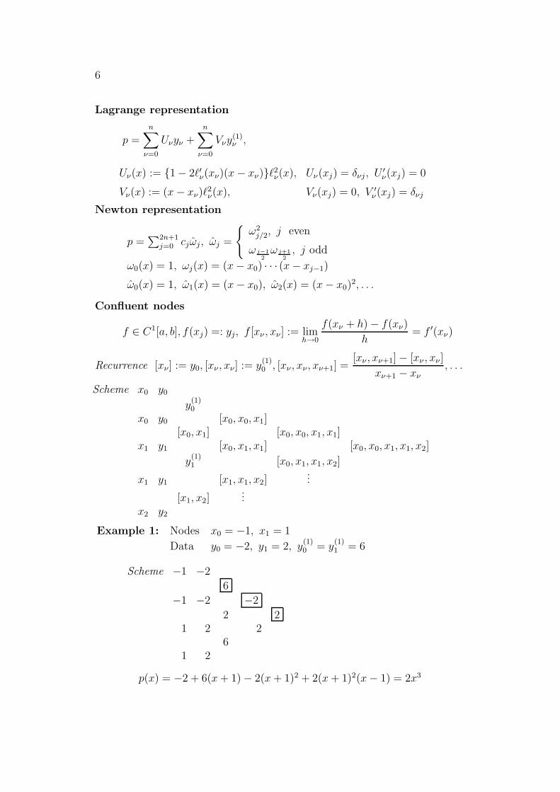
Example 1: Nodes x0 = −1, x1 = 1
Data y0 = −2, y1 = 2, y(1)0 = y
(1)1 = 6
Scheme −1 −2
6
−1 −2 −2
2 21 2 2
61 2
p(x) = −2 + 6(x+ 1)− 2(x+ 1)2 + 2(x+ 1)2(x− 1) = 2x3
1. GENERAL INTERPOLATION PROBLEM 7
Example 2: Nodes x0 = −1, x1 = 1
Data y0 = −2, y1 = 2, y(1)1 = 6, y
(2)1 = 12
f [xν, xν, xν ] :=f ′′(xν)
2!
Scheme −1 −2
2
1 2 2
6 21 2 12
2
61 2
p(x) = −2 + 2(x + 1) + 2(x+ 1)(x− 1) + 2(x+ 1)(x− 1)2 = 2x3
The Peano–Sard representation
Integral representation of a linear functional R (see Peano: Numer. Math. I)Functional J : Cm+1[a, b] → �
Functional L : C[a, b] → �
Functional R := J − LOrder m, i.e., Rp = 0 for all p ∈ PmExamples: Interpolation, divided differences, differentiation, quadrature, . . .
Theorem 1.2 (Peano–Sard)The linear functional R of order m applied to f ∈ Cm+1[a, b] satisfies
Rf =
∫ b
a
G(t)f (m+1)(t)dt,
where
G(t) = Rvt, vt(x) :=(x− t)m+m!
denotes the corresponding Peano kernel.If G(t) is definite in [a, b], then it holds (a < ξ < b)
Rf = cmf(m+1)(ξ), cm =
∫ b
a
G(t)dt =1
(m + 1)!Rhm+1.
Proof is given later for the special case of divided differences. �
8
Remarks
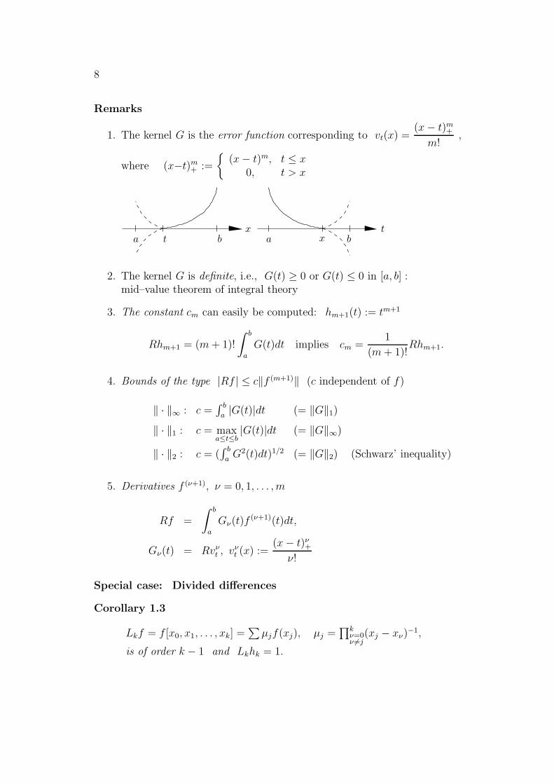
1. The kernel G is the error function corresponding to vt(x) =(x− t)m+m!
,
where (x−t)m+ :=
{(x− t)m, t ≤ x
0, t > x
PSfrag replacements
a t bx
a x bt
2. The kernel G is definite, i.e., G(t) ≥ 0 or G(t) ≤ 0 in [a, b] :mid–value theorem of integral theory
3. The constant cm can easily be computed: hm+1(t) := tm+1
Rhm+1 = (m+ 1)!
∫ b
a
G(t)dt implies cm =1
(m+ 1)!Rhm+1.
4. Bounds of the type |Rf | ≤ c‖f (m+1)‖ (c independent of f)
‖ · ‖∞ : c =∫ ba|G(t)|dt (= ‖G‖1)
‖ · ‖1 : c = maxa≤t≤b
|G(t)|dt (= ‖G‖∞)
‖ · ‖2 : c = (∫ baG2(t)dt)1/2 (= ‖G‖2) (Schwarz’ inequality)
5. Derivatives f (ν+1), ν = 0, 1, . . . , m
Rf =
∫ b
a
Gν(t)f(ν+1)(t)dt,
Gν(t) = Rvνt , vνt (x) :=
(x− t)ν+ν!
Special case: Divided differences
Corollary 1.3
Lkf = f [x0, x1, . . . , xk] =∑µjf(xj), µj =
∏kν=0ν 6=j
(xj − xν)−1,
is of order k − 1 and Lkhk = 1.
1. GENERAL INTERPOLATION PROBLEM 9
Proof: Interpolation polynomial pf of f with respect to x0, . . . , xk−1 :w(x) = (x− x0) · · · (x− xk−1), xk 6= x1, . . . , xk−1
Error (Numer. Math. I): f(xk)− pf(xk) = f [x0, . . . , xk−1, xk]w(xk)︸ ︷︷ ︸6=0
` ≤ k − 1 : f = h` =⇒ pf = h` =⇒ Lkh` = 0
f = hk =⇒ pf = hk − w since hk − w ∈ Pk−1
and pf(xν) = hk(xν)− w(xν) = hk(xν), ν = 0, . . . , k − 1
=⇒ hk(xk)− pf(xk) = w(xk) =⇒ Lkhk = 1 �
Corollary 1.4 Lk operating on the subspace Ck[a, b] satisfies
Lkf =
∫ b
a
G(t)f (k)(t)dt, G(t) = Lkvt, vt(x) =(x− t)k−1
+
(k − 1)!.
Proof: Taylor expansion in a using the integral remainder term: f = pk−1 +Rk
Rk(x) =
∫ b
a
f (k)(t)(x− t)k−1
+
(k − 1)!dt =
∫ b
a
f (k)(t)vt(x)dt
Lkf = Lkpk−1︸ ︷︷ ︸=0
+LkRk =
k∑
j=0
µjRk(xj) =
k∑
j=0
µj
∫ b
a
f (k)(t)vt(xj)dt
=
∫ b
a
f (k)(t)
k∑
j=0
µjvt(xj)
︸ ︷︷ ︸=Lkvt=:G(t)
dt. �
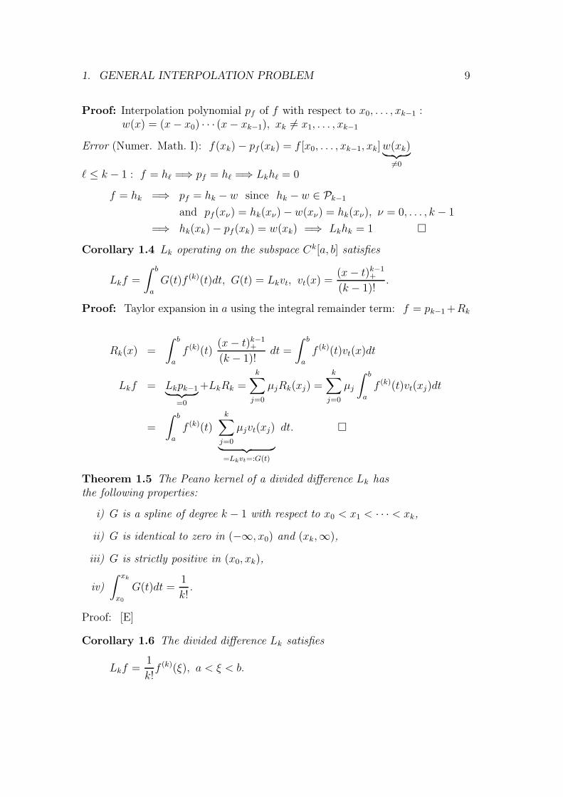
Theorem 1.5 The Peano kernel of a divided difference Lk hasthe following properties:
i) G is a spline of degree k − 1 with respect to x0 < x1 < · · · < xk,
ii) G is identical to zero in (−∞, x0) and (xk,∞),
iii) G is strictly positive in (x0, xk),
iv)
∫ xk
x0
G(t)dt =1
k!.
Proof: [E]
Corollary 1.6 The divided difference Lk satisfies
Lkf =1
k!f (k)(ξ), a < ξ < b.

10
Supplementary Examples – No. 1
Interpolation, extrapolation and approximation
Polynomials of higher order are not appropriate for extrapolationGiven: Number of the population in the USA from 1900 to 1990 every 10 yearsWanted: Prognosis for the year 1995 and 2000Material of data: Number of population in Millions
1900 1910 1920 1930 1940 1950 1960 1970 1980 1990
75.995 91.972 105.711 123.203 131.696 150.697 179.323 203.212 226.505 248.7
Different possibilities:
a) The interpolation polynomial p9(x) with respect to the nodes1900, 1910, . . . , 1990.
b) The construction of an interpolant cubic spline s(x) with respect tothese nodes and data.
c) The construction of polynomials pj(x), j = 1, . . . , 8, by the principle ofthe least squares of errors.
For each case the values are extrapolated for 1995 and 2000, i.e., thefunctions pj(x), j = 1, . . . , 9, and s(x) are evaluated at 1995 and 2000.
Numerical results order 3
order 1995 20001 249.79 259.402 264.96 279.333 264.86 279.154 254.94 257.985 253.70 254.636 268.87 305.037 277.08 337.328 185.48 -77.129 243.33 218.13cubic spline 258.39 266.62exact value 263.8 273.8
1900 1920 1940 1960 1980 20000
50
100
150
200
250
300
mill
ion
* exact values
Commentsp9(x) shows zigzag behaviour between 1980 and 2010;p8(x) shows shortly before 2000 a zero point (i.e., the population of USA is zero);p7(x) and p6(x) show an extreme increase after 1995;p5(x) and p4(x) show a maximal point at 1995 and then falling down;p3(x) and p2(x) show the realistic behaviour, as well as the cubic spline s(x).

2. TRIGONOMETRIC INTERPOLATION 11
2 Trigonometric Interpolation
Periodic processes
All arguments are equivalent → uniformly spaced nodes
Haar system {1, cosx, sin x, . . . , cosmx} in [0, 2π)
Dimension 2m+ 1 (odd)
Trigonometric polynomial T (x) =α0
2+
m∑
ν=1
{αν cos νx + βν sin νx}
Degree m
Πm : space of trigonometric polynomials of degree ≤ m
Orthogonality
∫ 2π
0
cos kxsin kx
� cos `xsin `x
dx = 0, k 6= `
Fourier coefficientsανβν
}=
1
π
∫ 2π
0
f(x)cos νxsin νx
dx
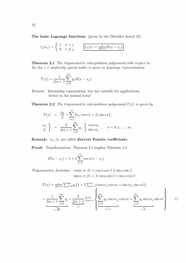
Dirichlet kernel D(u) := sin2m+1
2 u
sin 12u, u ∈ �
(m ≥ 1)
D(0) = 2m + 1 (l’Hospital)
D(
2(ν−j)π2m+1
)= 0, ν 6= j (ν, j ∈ � )
D(u) = 1 + 2 cos u+ · · ·+ 2 cosmu
Figure: m = 5
−π πu
y=D(u)
Interpolation problem
I. Odd number of uniformly spaced nodes
Given: Nodes xj = 2jπ2m+1
, j = 0, 1, . . . , 2m
Data yj ∈�, j = 0, 1, . . . , 2m (f ∈ C2π, yj := f(xj))
Wanted: T ∈ Πm satisfying T (xj) = yj, j = 0, 1, . . . , 2m
The unique solvability for arbitrary nodes in [0, 2π) (Haar space) is given.
12
The basic Lagrange functions (given by the Dirichlet kernel D):
tj(xν) =
{1, ν = j0, ν 6= j
tj(x) := 12m+1
D(x− xj)
Theorem 2.1 The trigonometric interpolation polynomial with respect tothe 2m+ 1 uniformly spaced nodes is given in Lagrange representation
T (x) =1
2m+ 1
2m∑
j=0
yjD(x− xj).
Remark: Interesting represention, but not suitable for applications,better in the normal form!
Theorem 2.2 The trigonometric interpolation polynomial T (x) is given by
T (x) =α0
2+
m∑
ν=1
{αν cos νx + βν sin νx},
ανβν
}=
2
2m+ 1
2m∑
j=0
yj
{cos νxjsin νxj
, ν = 0, 1, . . . , m.
Remark: αν, βν are called discrete Fourier coefficients.
Proof: Transformation: Theorem 2.1 implies Theorem 2.2
D(x− xj) = 1 + 2
m∑
ν=1
cos ν(x− xj)
Trigonometric formulas: cos(α± β) = cosα cos β ∓ sinα sin β
sin(α± β) = ± cosα sin β + sinα cos β
T (x) = 12m+1
∑2mj=0 yj{1 + 2
∑mν=1(cos νxj cos νx + sin νxj sin νx)}
=1
2m+ 1
2m∑
j=0
yj
︸ ︷︷ ︸=:
α02
+2
2m+ 1︸ ︷︷ ︸↪→
∑mν=1
2m∑
j=0
yj cos νxj
︸ ︷︷ ︸=:αν
cos νx +2m∑
j=0
yj sin νxj
︸ ︷︷ ︸=:βν
sin νx
�
2. TRIGONOMETRIC INTERPOLATION 13
Corollary 2.3 The relations of discrete orthogonality are satisfied
22m+1
2m∑j=0
cos kxj cos `xj =
2, k = ` = 0
1, k = ` 6= 0
0, k 6= `
(0 ≤ k, ` ≤ m)
22m+1
2m∑j=0
sin kxj sin `xj =
1, k = `
0, k 6= `(1 ≤ k, ` ≤ m)
22m+1
2m∑j=0
cos kxj sin `xj = 0 (0 ≤ k, ` ≤ m)
Proof: Interpolation of the basic functions 1, cos x, sin x, . . . , cosmx, sinmx. �
II. Even number of uniformly spaced nodes
Nodes xj =jπ
m, j = 0, 1, . . . , 2m− 1
Data yj ∈�, j = 0, 1, . . . , 2m− 1
Space {1, cos x, sin x, . . . , cosmx}, dim = 2m
(sinmx is omitted, since sinmxj = 0 for j = 0, 1, . . . , 2m− 1)
Haar system in {x0, . . . , x2m−1}(solvability of the interpolation problem for these special nodes)
The basic Lagrange functions tj(x) =1
2m
sinm(x− xj)tan
x−xj2
, j = 0, 1, . . . , 2m− 1
Compared to the Dirichlet kernel:sinmu
tan 12u
= D(u)− cosmu.
According to the Lagrange representation the normal representation follows.
Theorem 2.4 The trigonometric interpolation polynomial with respect tothe 2m uniformly spaced nodes is given by
T (x) =α0
2+
m∑
ν=1
′{αν cos νx + βν sin νx}(
Σ′ :αm2
),
ανβν
}=
1
m
2m−1∑
j=0
yj
{cos νxjsin νxj
, ν = 0, 1, . . . , m (β0 = βm = 0).
14
Exponential representation (more compact, data yj ∈ � ):
Space {e−imx, . . . , 1, . . . , eimx} Haar system in [0, 2π), dim = 2m+ 1
T (x) = α0
2+
m∑ν=1
{αν cos νx + βν sin νx} =m∑
ν=−maνe
iνx
a±ν = 12(αν ∓ iβν) (eix = cosx + i sin x)
Interpolation with 2m + 1 nodes:
a±ν =1
2m + 1
2m∑
j=0
yje∓iνxj
z = eix : T (x) = z−m2m∑ν=0
aν−mzν =: z−mS(z)
S(z) complex algebraic polynomial of degree ≤ 2m.
Idea: It is easier to determine S(z) than T (x), i.e.,the coefficients a±ν are simpler than αν and βν .
New interpolation problem
Space {1, eix, . . . , ei(n−1)x} : Haar system in [0, 2π), dim = n
Complex trigonometric polynomial R(x) =
n−1∑
ν=0
bνeiνx
Complex algebraic polynomial S(z) =n−1∑
ν=0
bνzν
z = eix
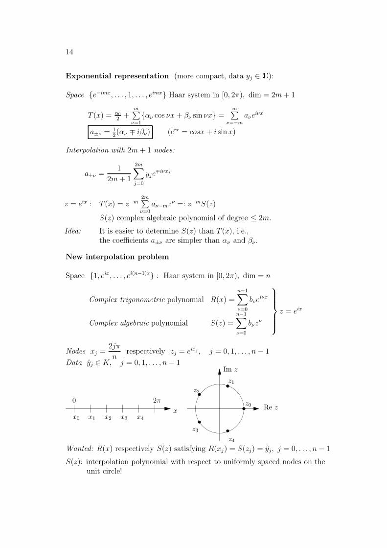
Nodes xj =2jπ
nrespectively zj = eixj , j = 0, 1, . . . , n− 1
Data yj ∈ K, j = 0, 1, . . . , n− 1
PSfrag replacements
x0 x1 x2 x3 x4
2π
x
0
z3
z4
z0
z1
z2
Re z
Im z
Wanted: R(x) respectively S(z) satisfying R(xj) = S(zj) = yj, j = 0, . . . , n− 1
S(z): interpolation polynomial with respect to uniformly spaced nodes on theunit circle!
2. TRIGONOMETRIC INTERPOLATION 15
Relations of the nodes: zj = e2ijπn , zνj = e
2ijνπn
znj = 1, z0j = zν0 = 1, zνj = zjν , zj = z−j, z
−kj = zn−kj
0 = znj − 1 = (zj − 1)︸ ︷︷ ︸6=0,j 6=0
n−1∑
ν=0
zνj
︸ ︷︷ ︸=0,j 6=0
,n−1∑
ν=0
zνj =
0, j 6= 0
n, j = 0
Orthogonality1
n
n−1∑
ν=0
zjνz−kν =
{0, j 6= k1, j = k
Basic functions Sk(z) :=1
n
n−1∑
ν=0
(z−kz)ν with Sk(zj) = δkj
Lagrange representation S(z) =n−1∑
k=0
ykSk(z)
Theorem 2.5 The complex trigonometric interpolation polynomial R(x)respectively the complex algebraic interpolation polynomial S(z) with respectto the nodes xj = 2jπ
nrespectively zj = eixj ∈ K (j = 0, 1, . . . , n− 1) and
the data yj (j = 0, 1, . . . , n− 1) has the coefficients
bν =1
n
n−1∑
k=0
ykz−kν , ν = 0, 1, . . . , n− 1.
Proof: The Lagrange representation implies the statement
S(z) =
n−1∑
k=0
ykSk(z) =
n−1∑
ν=0
1
n
n−1∑
k=0
ykzν−k
︸ ︷︷ ︸=bν
zν =
n−1∑
ν=0
bνzν . �
Relation between the coefficients bν and αν, βν :Assume that n = 2m = 2p (even number of uniformly spaced nodes)
αν
βν
=
1
m
n−1∑
j=0
yj
cos νxj
sin νxj, ν = 0, 1, . . . , m (βm = 0) (real)
bν =1
n
n−1∑
k=0
ykz−kν , ν = 0, 1, . . . , n− 1 (complex )
yk → yk

16
Backward transformation formulas
Consider the easier case of 2m+ 1 nodes (see above)
T (x) = z−mS(z), S(z) =
2m∑
ν=0
aν−mzν
a±ν =1
2(αν ∓ iβν)
aν =1
2(αnu− iβν), a−ν =
1
2(αnu+ iβν)
hence we have
αν = aν + a−ν, βν = i(aν + a−ν)
further
yj = T (xj) = z−mj S(zj) = z−mj yj → yj = yj · zmj
Summary: Trigonometric interpolation: n = 2m
Nodes xj = 2jπn
Data yj ∈ K
}j = 0, 1, . . . , n− 1
Trigonometric interpolation polynomial T (x) with coefficients
ανβν
}=
1
m
n−1∑
j=0
yj
{cos νxjsin νxj
, ν = 0, 1, . . . , m
Computation by the coefficients of the complex interpolation polynomial:
Nodes zj = ei2jπ/n
Data yj ∈ K
}j = 0, 1, . . . , n− 1
Complex interpolation polynomial S(z) =n−1∑
ν=0
bνzν , bν =
1
n
∑ykz−kν
Assume an even number of nodes n = 2mChoose the data yk → ykCompute the coefficients bν with the FFT method (see below).Then the coefficients αν, βν will follow for the real trigonometric interpolationpolynomial T (x) (→ backward transformation formulas).
3. FOURIER TRANSFORM 17
3 Fourier Transform
Space C2π, 〈f, g〉 :=1
π
∫ 2π
0
f(x)g(x)dx, L2–norm ‖f‖2 := 〈f, f〉1/2
Subspace Πm : { 1√2, cos x, sin x, . . . , cosmx, sinmx} ONS
Fourier series f ∼ α0
2+∞∑
ν=1
{αν cos νx + βν sin νx}
Fourier coefficientsανβν
}= 〈f, cos νx
sin νx〉 =
1
π
∫ 2π
0
f(x)
{cos νxsin νx
dx
Fourier polynomial Sm: the mth partial sum of the series
Complex–valued functions
Scalar product 〈f, g〉 :=1
2π
∫ 2π
0
f(x)g(x)dx
ONS (orthogonal normal system) {1, eix, . . . , ei(n−1)x}
Fourier series∞∑
ν=0
bνeiνx
Fourier coefficients bν =1
2π
∫ 2π
0
f(x)e−iνxdx
L2–approximation
Space C[a, b], ‖ · ‖2
Finite dimensional subspace U with an
orthogonal normal basis {ϕ0, ϕ1, . . . , ϕn−1}The best approximation g∗ ∈ U of f ∈ C, i.e.,
‖f − g∗‖2 ≤ ‖f − g‖2 for all g ∈ U
Existence, uniqueness, construction of p∗ ?
The best approximation g∗ =
n−1∑
ν=0
cνϕν, cν := 〈f, ϕν〉 the Fourier coefficients
Theorem 3.1 (Minimal property of the Fourier coefficients)The Fourier polynomial g∗ is the best L2–approximation of f ∈ C[a, b].
18
Proof: g ∈ U, g =n−1∑
ν=0
cνϕν
‖f − g‖22 = 〈f − g, f − g〉 = 〈f, f〉 − 2〈f, g〉+ 〈g, g〉
= ‖f‖22 − 2
∑
j
cj〈f, ϕj〉+∑
j
∑
k
cjck〈ϕj, ϕk︸ ︷︷ ︸=δjk
〉
= ‖f‖2 +∑
(c2j − 2cj cj + c2
j)−∑
c2j
= ‖f‖2 −∑
c2j︸ ︷︷ ︸
+∑
(cj − cj)2
= ‖f − g∗‖22 (insert g = g∗). �
Corollary 3.2 Sm is the best L2–approximation of f ∈ C2π, i.e.,
‖f − sm‖2 ≤ ‖f − tm‖2 for all tm ∈ Πm.
Computation of the Fourier coefficients
ανβν
}=
1
π
∫ 2π
0
f(x)
{cos νxsin νx
dx resp. bν =1
2π
∫ 2π
0
f(x)e−iνxdx
Quadrature formula: Periodic integrand, hence we choose uniformly spaced nodes
Trapezoidal rule: Nodes xj =2jπ
n, j = 0, 1, . . . , n, h =
2π
n
h2
(g(x0) + g((x1)) + · · ·+ h2
(g(xn−1) + g(xn)) =2π
n
n−1∑
j=0
g(xj),
ανβν
}=
2
n
n−1∑
j=0
f(xj)cos νxjsin νxj
+ error =
{ανβν
+ error
bν =1
2
n−1∑
j=0
f(xj)e−iνxj + error = bν + error
Discrete Fourier coefficients αν, βν, bν
Trapezoidal Σ = mid–point Σ = arithmetic Σ
Remark: The trapezoidal rule is very convenient for periodic functions(because of high order of approximation) (Euler–MacLaurin §6).
Result 3.3 The Fourier coefficients αν, βν and bν (see above) are very goodapproximated by the discrete Fourier coefficients αν, βν and bν .
3. FOURIER TRANSFORM 19
Remark: The discrete Fourier coefficients are the coefficients of the trigonometricrespectively complex algebraic interpolation polynomial T (x)(Theorem 2.2, 2.4) resp. S(z) (Theorem 2.5).
The discrete Fourier evaluation
Space C2π : nodes xj =2jπ
n, j = 0, 1, . . . , n− 1 (n = 2m+ 1 or n = 2m)
〈f, g〉n :=2
n
n−1∑
j=0
f(xj)g(xj) (arithmetic Σ of 〈f, g〉)
discrete analogon to 〈f, g〉, not a scalar product in C2π,
because of the missing definiteness!
Seminorm ‖f‖2,n := 〈f, f〉1/2n .
Space Πk (0 ≤ k ≤ m, where m :=[n
2
]: 〈f, g〉n is a semi scalar product,
hence the discrete Fourier polynomial Tk(x) with αν and βν (Th. 3.1).
Analogously: ONS {1, eix, . . . , ei(n−1)x}
〈f, g〉n :=1
n
n−1∑
j=0
f(xj)g(xj)
Least square problem
Given: Nodes xj =2jπ
n, j = 0, 1, . . . , n− 1 (n = 2m+ 1 or n = 2m)
Data yj (yj := f(xj), f ∈ C2π), j = 0, 1, . . . , n− 1
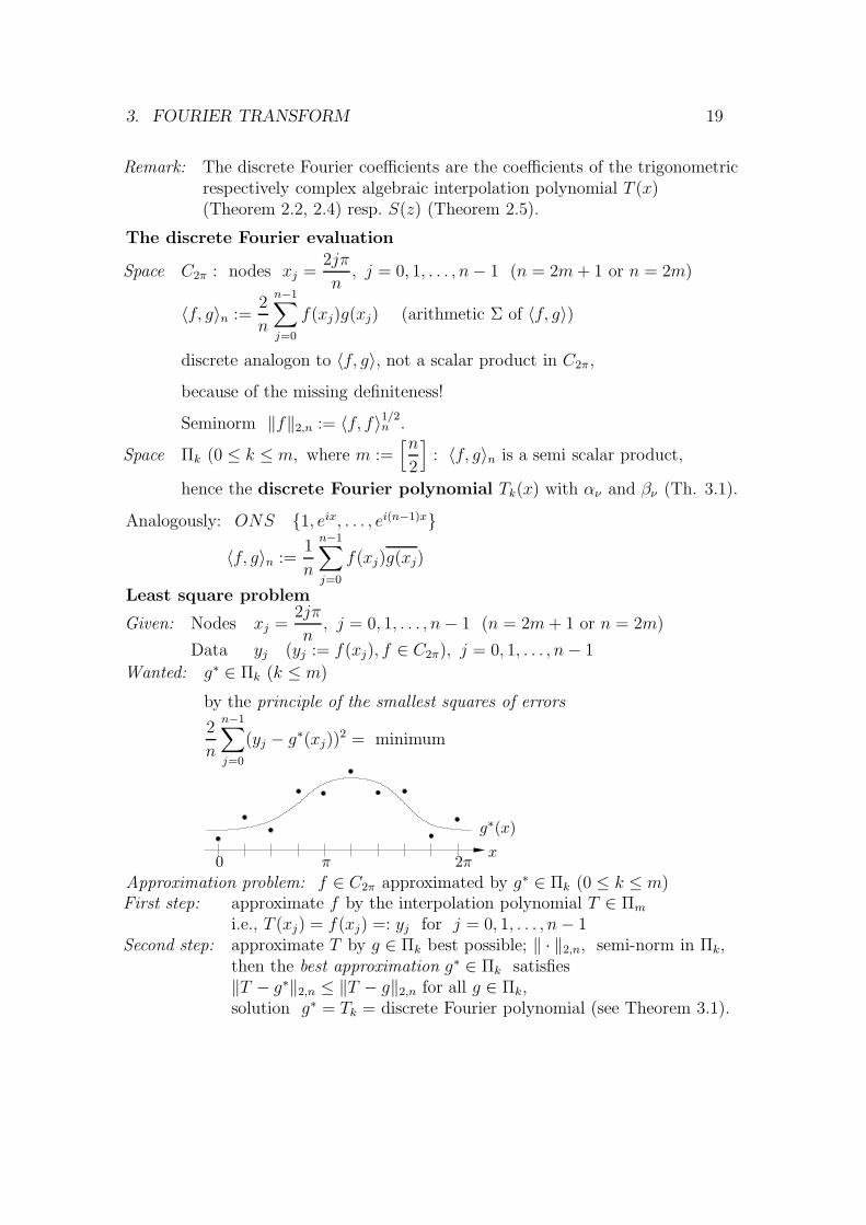
Wanted: g∗ ∈ Πk (k ≤ m)
by the principle of the smallest squares of errors
2
n
n−1∑
j=0
(yj − g∗(xj))2 = minimum
PSfrag replacements
0 π 2πx
g∗(x)
Approximation problem: f ∈ C2π approximated by g∗ ∈ Πk (0 ≤ k ≤ m)First step: approximate f by the interpolation polynomial T ∈ Πm
i.e., T (xj) = f(xj) =: yj for j = 0, 1, . . . , n− 1Second step: approximate T by g ∈ Πk best possible; ‖ · ‖2,n, semi-norm in Πk,
then the best approximation g∗ ∈ Πk satisfies‖T − g∗‖2,n ≤ ‖T − g‖2,n for all g ∈ Πk,solution g∗ = Tk = discrete Fourier polynomial (see Theorem 3.1).
20
Theorem 3.4 The discrete Fourier polynomial Tk (k < m) equal to the k − thpartial polynomial of the interpolation polynomial Tm solves the given least squaresproblem.
Direct proof (without approximation theory):
F (α0, . . . , αk, β1, . . . , βk) :=
n−1∑
j=0
{1
2α0 +
k∑
ν=1
(αν cos νxj + βν sin νxj)− f(xj)
}2
Necessary conditions:
the discrete Fourier coefficients αν can be computed by∂F
∂αν= 0, ν = 0, 1, . . . , k
the discrete Fourier coefficients βν can be computed by∂F
∂βν= 0, ν = 1, . . . , k
Remark: This is a very elegant solution!Compare the least squares problem for algebraic polynomials ∈ Pk,then the normal equations ATAx = AT b (linear system)has to be solved.
Scheme
Scalar productarithm. Σ−→ discrete semi scalar product
↓ ↓
Fourier evaluation
Fourier polynomial
discrete Fourier polynomial
= trigon. interpol. polynomial
↓ ↓Fourier coefficients
arithm. Σ−→ discrete Fourier coefficients
Supplementary Examples – No. 2
Fourier Series (Schwarz∗)
Example 1
“Roof” function f(x), 2π–periodic, f(x) = |x| in the basic interval [−π, π].a) Wanted: Fourier series of f(x): f(x) even, i.e., all βk = 0;
α0 =1
π
∫ π
−π|x|dx =
2
π
∫ π
0
xdx = π,
αk =2
π
∫ π
0
x cos kxdx =2
π
{1
kx sin kx}
∣∣∣∣π
0
− 1
k
∫ π
0
sin kxdx
}
=2
πk2cos kx
∣∣∣∣π
0
=2
πk2{(−1)k − 1}, k > 0.
3. FOURIER TRANSFORM 21
The Fourier series reads
f(x) ∼ 1
2π − 4
π
{cos x
12+
cos 3x
32+
cos 5x
52+ . . .
},
and hence it follows
1
12+
1
32+
1
52+
1
72+ · · · = π2
8.
Error estimation:
|f(x)− S25(x)| ≤ 4
π
∞∑
ν=13
1
(2ν + 1)2≤ 0.025.
b) Wanted: Trigon. interpolation polynomial (discrete Fourier polynomial)
T (x) =α0
2+
3∑
ν=0
(αν cos vx+ βv sin vx)
with respect to the nodes xj = jπ4
and data yj = f(xj), j = 0, 1, . . . , 7.The discrete Fourier coefficients read
α0 = π, α1 = −1.34, α2 = 0, α3 = −0.23, α4 = 0, β1 = β2 = β3 = 0.
Compare with the classical Fourier coefficients
α0 = π, α1 = −1.27, α2 = 0, α3 = −0.14, α4 = 0, β1 = β2 = β3 = 0.
Notice that T (0) = 0 (interpolation) and S25(0) = 0.0244 (trapezoidal sum) hold.
Example 2
The function x→ x2, 0 ≤ x < 2π, will be continued periodically by f(x).
Wanted: Fourier series of f(x): Integration by parts
α0 =1
π
∫ 2π
0
x2dx =8π2
3,
αk =1
π
∫ 2π
0
x2 cos kxdx =4
k2, k = 1, 2, . . . ,
βk =1
π
∫ 2π
0
x2 sin kxdx = −4π
k, k = 1, 2, . . . .
The Fourier series reads
4π2
3+∞∑
k=1
{4
k2cos kx− 4π
ksin kx
}.
22
Computation of the discrete Fourier coefficients
ανβν
}=
2
n
n−1∑
j=0
yj
{cos νxjsin νxj
ν = 0, 1, . . . ,[n
2
]
In general (Theorem 2.5):
bk =1
n
n−1∑
j=0
yjz−kj Fourier analysis
(k = 0, 1, . . . , n− 1)
yk =
n−1∑
j=0
bjzkj Fourier synthesis
Fast Fourier Transform (FFT)
Computational costs for the n complex algebraic sums: n = 2p (p ∈ � )
Horner ∼ 2n2 arithmetic operations (n · 2p+1)FFT ∼ n log2 n arithmetic operations (n · p)
FFT: Algorithm of Cooley & Tukey 1965(see Stoer I; Schwarz)
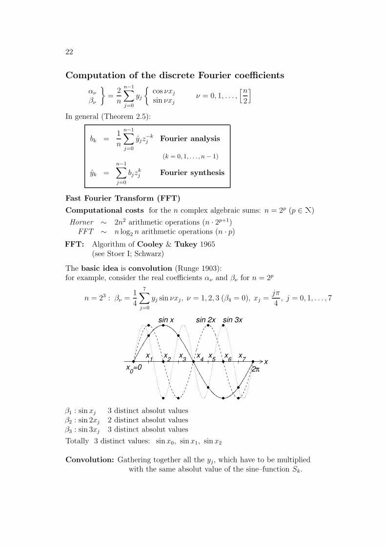
The basic idea is convolution (Runge 1903):for example, consider the real coefficients αν and βν for n = 2p
n = 23 : βν =1
4
7∑
j=0
yj sin νxj, ν = 1, 2, 3 (β4 = 0), xj =jπ
4, j = 0, 1, . . . , 7
x0=0
x2 x
3 x
4 x
5 x
6 x
7
2π x
sin x sin 2x sin 3x
x1
β1 : sin xj 3 distinct absolut valuesβ2 : sin 2xj 2 distinct absolut valuesβ3 : sin 3xj 3 distinct absolut values
Totally 3 distinct values: sin x0, sin x1, sin x2
Convolution: Gathering together all the yj, which have to be multipliedwith the same absolut value of the sine–function Sk.
3. FOURIER TRANSFORM 23
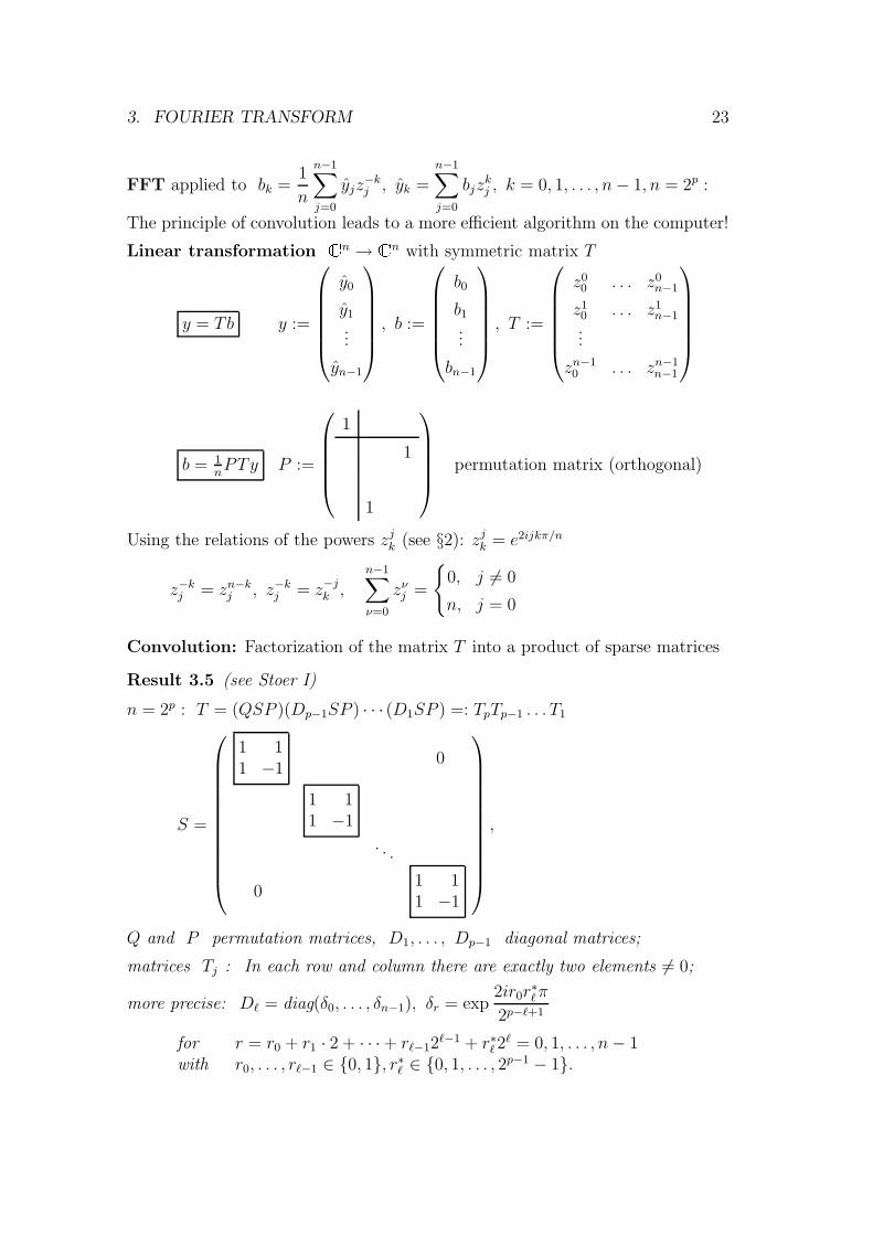
FFT applied to bk =1
n
n−1∑
j=0
yjz−kj , yk =
n−1∑
j=0
bjzkj , k = 0, 1, . . . , n− 1, n = 2p :
The principle of convolution leads to a more efficient algorithm on the computer!
Linear transformation � n → � n with symmetric matrix T
y = Tb y :=
y0
y1
...
yn−1
, b :=
b0
b1
...
bn−1
, T :=
z00 . . . z0
n−1
z10 . . . z1
n−1...
zn−10 . . . zn−1
n−1
b = 1nPTy P :=
1
1
1
permutation matrix (orthogonal)
Using the relations of the powers zjk (see §2): zjk = e2ijkπ/n
z−kj = zn−kj , z−kj = z−jk ,n−1∑
ν=0
zνj =
{0, j 6= 0
n, j = 0
Convolution: Factorization of the matrix T into a product of sparse matrices
Result 3.5 (see Stoer I)
n = 2p : T = (QSP )(Dp−1SP ) · · · (D1SP ) =: TpTp−1 . . . T1
S =
1 11 −1
0
1 11 −1
. . .
01 11 −1
,
Q and P permutation matrices, D1, . . . , Dp−1 diagonal matrices;
matrices Tj : In each row and column there are exactly two elements 6= 0;
more precise: D` = diag(δ0, . . . , δn−1), δr = exp2ir0r
∗`π
2p−`+1
for r = r0 + r1 · 2 + · · ·+ r`−12`−1 + r∗`2` = 0, 1, . . . , n− 1
with r0, . . . , r`−1 ∈ {0, 1}, r∗` ∈ {0, 1, . . . , 2p−1 − 1}.
24
P defined by x = Px with
xk+j·2 = xj+k·2p−1 for k = 0, 1 and j = 0, 1, . . . , 2p−1 − 1;
Q defined by x = Qx with
xj0+j1·2+···+jp−12p−1 = xjp−1+jp−2·2+···+j0·2p−1 for j0, . . . , jp−1 = 0, 1.
Without proof �
FFT (fast computation): y = Tp(Tp−1 . . . (T2(T1b)) . . . )
b =: v1 → T1v1 =: v2 → T2v2 =: v3 → . . . → Tpvp = y↑ ↑ ↑ ↑
convolution
Realization: Tjvj = DjSPvj = Dj(S(Pvj))
Inversion: b = T−1y with T−1 = T−11 . . . T−1
p , T−1j =
1
2PSD−1
j
3. FOURIER TRANSFORM 25
Supplementary Examples – No. 3
Fast Fourier Transform (FFT)
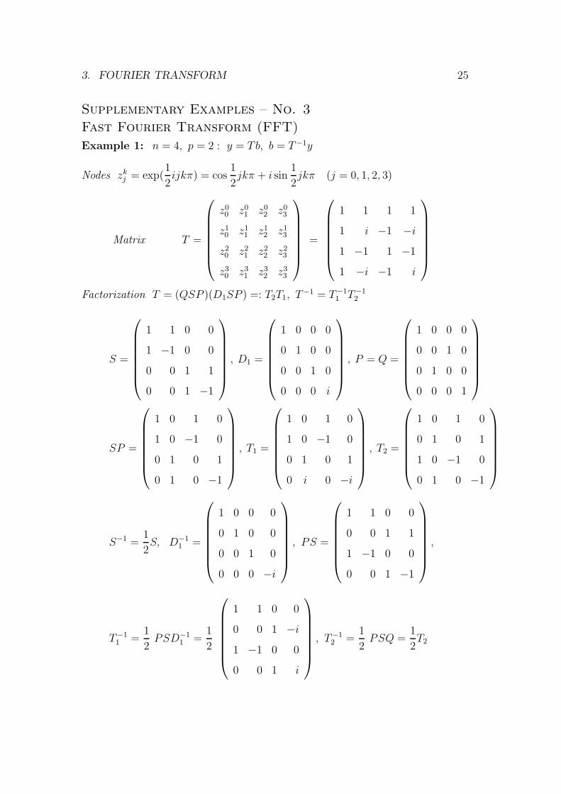
Example 1: n = 4, p = 2 : y = Tb, b = T−1y
Nodes zkj = exp(1
2ijkπ) = cos
1
2jkπ + i sin
1
2jkπ (j = 0, 1, 2, 3)
Matrix T =
z00 z0
1 z02 z0
3
z10 z1
1 z12 z1
3
z20 z2
1 z22 z2
3
z30 z3
1 z32 z3
3
=
1 1 1 1
1 i −1 −i1 −1 1 −1
1 −i −1 i
Factorization T = (QSP )(D1SP ) =: T2T1, T−1 = T−1
1 T−12
S =
1 1 0 0
1 −1 0 0
0 0 1 1
0 0 1 −1
, D1 =
1 0 0 0
0 1 0 0
0 0 1 0
0 0 0 i
, P = Q =
1 0 0 0
0 0 1 0
0 1 0 0
0 0 0 1
SP =
1 0 1 0
1 0 −1 0
0 1 0 1
0 1 0 −1
, T1 =
1 0 1 0
1 0 −1 0
0 1 0 1
0 i 0 −i
, T2 =
1 0 1 0
0 1 0 1
1 0 −1 0
0 1 0 −1
S−1 =1
2S, D−1
1 =
1 0 0 0
0 1 0 0
0 0 1 0
0 0 0 −i
, PS =
1 1 0 0
0 0 1 1
1 −1 0 0
0 0 1 −1
,
T−11 =
1
2PSD−1
1 =1
2
1 1 0 0
0 0 1 −i1 −1 0 0
0 0 1 i
, T−1
2 =1
2PSQ =
1
2T2
26
Convolutions
Y = Tb : b −→ v = T1b −→ y = T2v
b0 v0 = b0 + b2 y0 = v0 + v2 = b0 + b1 + b2 + b3
b1 v1 = b0 − b2 y1 = v1 + v3 = b0 + ib1 − b2 + ib3
b2 v2 = b1 + b3 y2 = v0 − v2 = b0 − b1 + b2 − b3
b3 v3 = i(b1 − b3) y3 = v1 − v3 = b0 − ib1 − b2 + ib3
b = T−1y : y −→ w = T−12 y −→ b = T−1
1 w
y0 w0 = 12(y0 + y2) b0 = 1
2(w0 + w1) = 1
4(y0 + y1 + y2 + y3)
y1 w1 = 12(y1 + y3) b1 = 1
2(w2 − iw3) = 1
4(y0 − iy1 − y2 + iy3)
y2 w2 = 12(y0 − y2) b2 = 1
2(w0 − w1) = 1
4(y0 − y1 + y2 − y3)
y3 w3 = 12(y1 − y3) b3 = 1
2(w2 + iw3) = 1
4(y0 + iy1 − y2 − iy3)
Costs: 9 operations (np = 8) comp. to 28 operations (n2p+1 = 32) for Tb.
Backward transformation to the αν and βν is possible.
Example 2: Trigonometric interpolation of f(x) = cos 4x with respect to the
nodes xj = jπ4, j = 0, 1, . . . , 7.
Wanted: The discrete Fourier coefficients in the representation
T (x) =α0
2+
3∑
ν=1
(αnu cos νx + βν sin νx) +α4
2cos 4x.
The function values are f(xj) = (−1)j, j = 0, 1, . . . , 4.Choose yk := f(x2k) + if(x2k+1) = 1− i for k = 0, 1, 2, 3, then the
complex polynomial S(z) has the coefficinets
bν =1
4
3∑
k=0
ykz−kν , ν = 0, 1, 2, 3.
FFT yields
b0 = 1− i, b1 = b2 = b3 = 0, i.e., S(z) = b0 = yk.
Backward transformation yields the discrete Fourier coefficients
α0 = α1 = α2 = α3 = β1 = β2 = β3 = 0 and α4 = 2, i.e., T (x) = cos 4x.
4. CUBIC SPLINE INTERPOLATION 27
4 Cubic Spline Interpolation
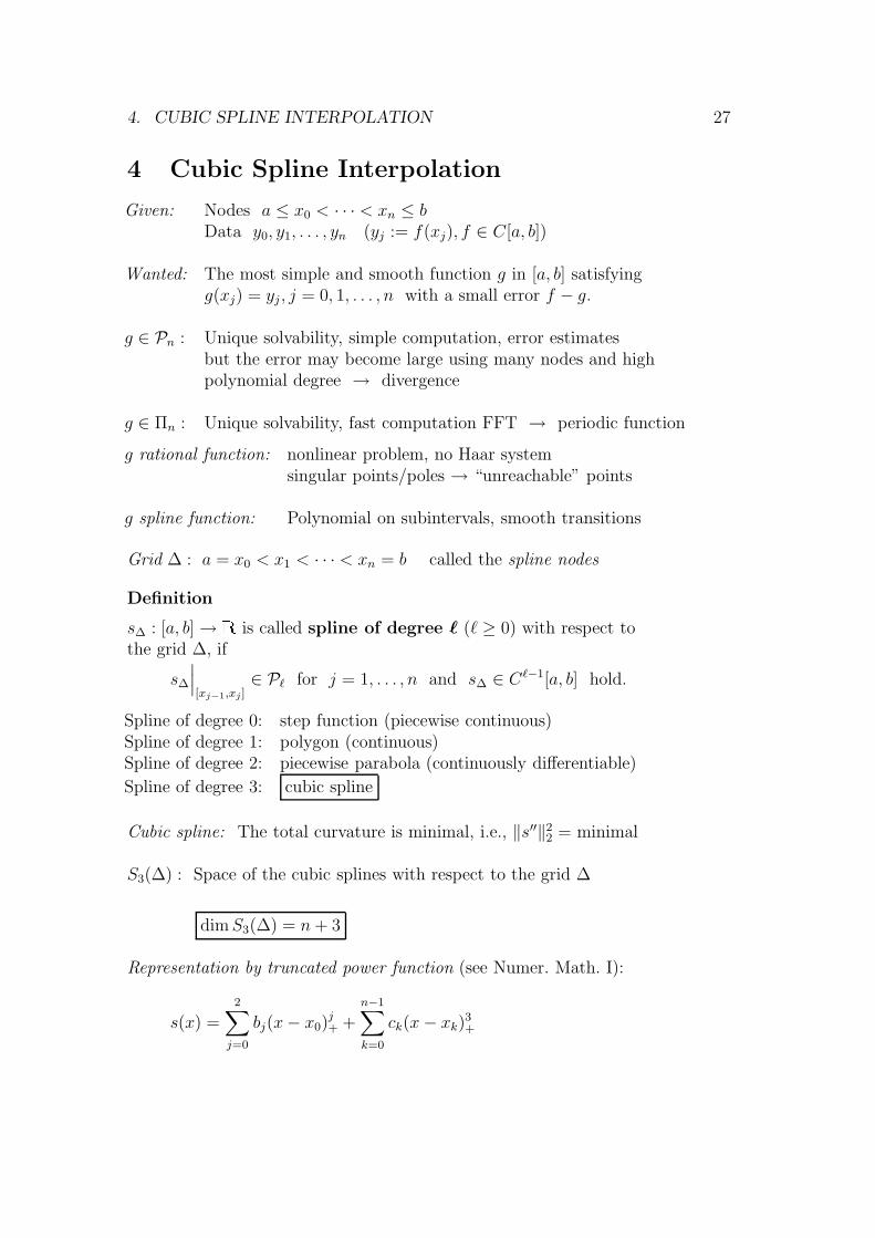
Given: Nodes a ≤ x0 < · · · < xn ≤ bData y0, y1, . . . , yn (yj := f(xj), f ∈ C[a, b])
Wanted: The most simple and smooth function g in [a, b] satisfyingg(xj) = yj, j = 0, 1, . . . , n with a small error f − g.
g ∈ Pn : Unique solvability, simple computation, error estimatesbut the error may become large using many nodes and highpolynomial degree → divergence
g ∈ Πn : Unique solvability, fast computation FFT → periodic function
g rational function: nonlinear problem, no Haar systemsingular points/poles → “unreachable” points
g spline function: Polynomial on subintervals, smooth transitions
Grid ∆ : a = x0 < x1 < · · · < xn = b called the spline nodes
Definition
s∆ : [a, b]→ �is called spline of degree ` (` ≥ 0) with respect to
the grid ∆, if
s∆
∣∣∣[xj−1,xj ]
∈ P` for j = 1, . . . , n and s∆ ∈ C`−1[a, b] hold.
Spline of degree 0: step function (piecewise continuous)Spline of degree 1: polygon (continuous)Spline of degree 2: piecewise parabola (continuously differentiable)
Spline of degree 3: cubic spline
Cubic spline: The total curvature is minimal, i.e., ‖s′′‖22 = minimal
S3(∆) : Space of the cubic splines with respect to the grid ∆
dimS3(∆) = n+ 3
Representation by truncated power function (see Numer. Math. I):
s(x) =2∑
j=0
bj(x− x0)j+ +n−1∑
k=0
ck(x− xk)3+
28
Representation interval by interval
s(x) =
p0(x) in [x0, x1]p1(x) in [x1, x2]...pn−1(x) in [xn−1, xn]
p0, p1, . . . , pn−1 ∈ P3.
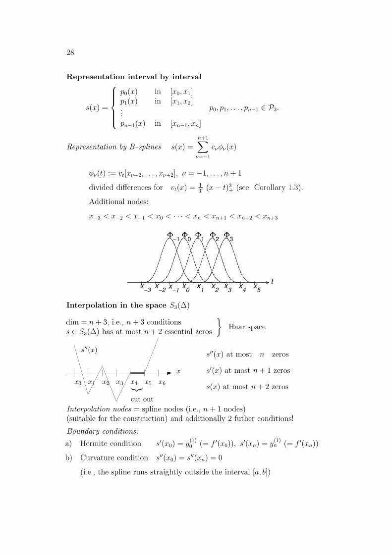
Representation by B–splines s(x) =
n+1∑
ν=−1
cνφν(x)
φν(t) := vt[xν−2, . . . , xν+2], ν = −1, . . . , n+ 1
divided differences for vt(x) = 13!
(x− t)3+ (see Corollary 1.3).
Additional nodes:
x−3 < x−2 < x−1 < x0 < · · · < xn < xn+1 < xn+2 < xn+3
x−3
x−2
x0 x
1 x
2 x
3 x
4 x
5 t
Φ−1
Φ0 Φ
2 Φ
3
x−1
Φ1
Interpolation in the space S3(∆)
dim = n + 3, i.e., n + 3 conditionss ∈ S3(∆) has at most n+ 2 essential zeros
}Haar space
PSfrag replacements
x0 x1 x2 x3 x4 x5 x6
x
s′′(x)
︸︷︷︸cut out
s′′(x) at most n zeros
s′(x) at most n+ 1 zeros
s(x) at most n + 2 zeros
Interpolation nodes = spline nodes (i.e., n + 1 nodes)(suitable for the construction) and additionally 2 futher conditions!
Boundary conditions:
a) Hermite condition s′(x0) = y(1)0 (= f ′(x0)), s′(xn) = y
(1)n (= f ′(xn))
b) Curvature condition s′′(x0) = s′′(xn) = 0
(i.e., the spline runs straightly outside the interval [a, b])

4. CUBIC SPLINE INTERPOLATION 29
Definition sf ∈ S3(∆) with sf (xj) = yj (= f(xj)), j = 0, 1, . . . , n,
is called interpolating spline of f with respect to ∆.
Theorem 4.1 The interpolating cubic spline sf with boundary condition (a)or (b) has the following representation in the subinterval [xj−1, xj] of length hj(j = 1, . . . , n):
sf(x) =1
6hj
{Mj(x− xj−1)3 +Mj−1(xj − x)3
}+ bj(x−
xj + xj−1
2) + aj
with the coefficients
aj =yj + yj−1
2− 1
12h2j(Mj +Mj−1),
bj =yj − yj−1
hj− 1
6hj(Mj −Mj−1),
and with the moments Mj given by the linear system (of dimn + 1 resp. n− 1)
h1
3h1
60
h1
6h1+h2
3h2
6. . .
. . .hn−1
6hn−1+hn
3hn6
0 hn6
hn3
M0
M1......
Mn−1
Mn
=
m0
m1......
mn−1
mn
and with
m0 =y1 − y0
h1− y(1)
0 , mn = −yn − yn−1
hn+ y(1)
n ,
mj =yj+1 − yjhj+1
− yj − yj−1
hj, j = 1, . . . , n− 1.
Proof: Construction of the interpolating cubic spline
s′′: polygon: linear interpolation between the nodes, hj := xj − xj−1
moments Mj := s′′(xj), j = 0, 1, . . . , ny integration
s′: continuity in the nodes
y integration
s:continuity in the nodesand interpolation conditions
}=⇒ linear system for the moments
30
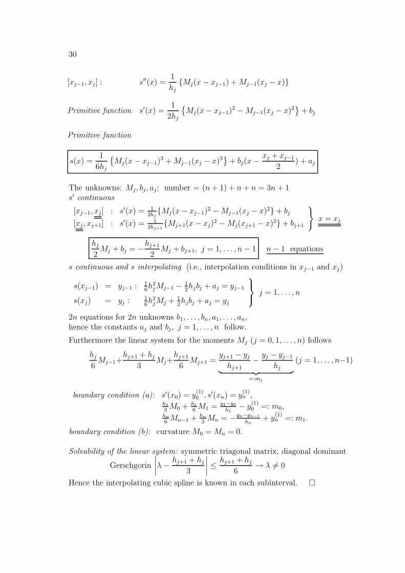
[xj−1, xj] : s′′(x) =1
hj{Mj(x− xj−1) +Mj−1(xj − x)}
Primitive function s′(x) =1
2hj
{Mj(x− xj−1)2 −Mj−1(xj − x)2
}+ bj
Primitive function
s(x) =1
6hj
{Mj(x− xj−1)3 +Mj−1(xj − x)3
}+ bj(x−
xj + xj−1
2) + aj
The unknowns: Mj, bj, aj; number = (n+ 1) + n+ n = 3n+ 1s′ continuous
[xj−1, xj] : s′(x) = 12hj{Mj(x− xj−1)2 −Mj−1(xj − x)2}+ bj
[xj, xj+1] : s′(x) = 12hj+1{Mj+1(x− xj)2 −Mj(xj+1 − x)2}+ bj+1
}x = xj
hj2Mj + bj = −hj+1
2Mj + bj+1, j = 1, . . . , n− 1 n− 1 equations
s continuous and s interpolating (i.e., interpolation conditions in xj−1 and xj)
s(xj−1) = yj−1 : 16h2jMj−1 − 1
2hjbj + aj = yj−1
s(xj) = yj : 16h2jMj + 1
2hjbj + aj = yj
j = 1, . . . , n
2n equations for 2n unknowns b1, . . . , bn, a1, . . . , an,hence the constants aj and bj, j = 1, . . . , n follow.
Furthermore the linear system for the moments Mj (j = 0, 1, . . . , n) follows
hj6Mj−1+
hj+1 + hj3
Mj+hj+1
6Mj+1 =
yj+1 − yjhj+1
− yj − yj−1
hj︸ ︷︷ ︸=:mj
(j = 1, . . . , n−1)
boundary condition (a): s′(x0) = y(1)0 , s′(xn) = y
(1)n ,
h1
3M0 + h1
6M1 = y1−y0
h1− y(1)
0 =: m0,hn6Mn−1 + hn
3Mn = −yn−yn−1
hn+ y
(1)n =: m1.
boundary condition (b): curvature M0 = Mn = 0.
Solvability of the linear system: symmetric triagonal matrix, diagonal dominant
Gerschgorin
∣∣∣∣λ−hj+1 + hj
3
∣∣∣∣ ≤hj+1 + hj
6→ λ 6= 0
Hence the interpolating cubic spline is known in each subinterval. �
4. CUBIC SPLINE INTERPOLATION 31
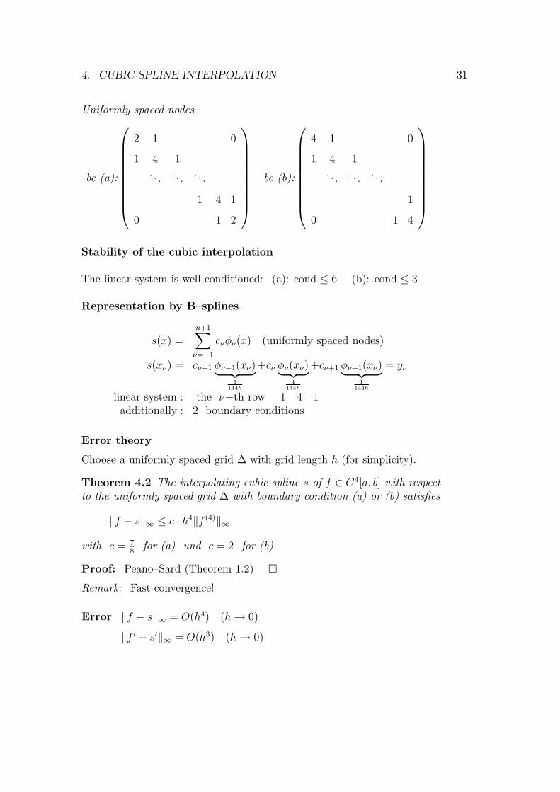
Uniformly spaced nodes
bc (a):
2 1 0
1 4 1. . .
. . .. . .
1 4 1
0 1 2
bc (b):
4 1 0
1 4 1. . .
. . .. . .
1
0 1 4
Stability of the cubic interpolation
The linear system is well conditioned: (a): cond ≤ 6 (b): cond ≤ 3
Representation by B–splines
s(x) =
n+1∑
ν=−1
cνφν(x) (uniformly spaced nodes)
s(xν) = cν−1 φν−1(xν)︸ ︷︷ ︸1
144h
+cν φν(xν)︸ ︷︷ ︸4
144h
+cν+1 φν+1(xν)︸ ︷︷ ︸1
144h
= yν
linear system : the ν−th row 1 4 1additionally : 2 boundary conditions
Error theory
Choose a uniformly spaced grid ∆ with grid length h (for simplicity).
Theorem 4.2 The interpolating cubic spline s of f ∈ C4[a, b] with respectto the uniformly spaced grid ∆ with boundary condition (a) or (b) satisfies
‖f − s‖∞ ≤ c · h4‖f (4)‖∞
with c = 78
for (a) und c = 2 for (b).
Proof: Peano–Sard (Theorem 1.2) �Remark: Fast convergence!
Error ‖f − s‖∞ = O(h4) (h→ 0)
‖f ′ − s′‖∞ = O(h3) (h→ 0)

32
Compare with the Cauchy remainder term in case of algebraic interpolation
‖f − pn‖∞ ≤‖ωn+1‖∞(n+ 1)!
‖f (n+1)‖∞
Tschebyscheff nodes
‖ωn+1‖∞ =1
2n→ 0
but maybe ‖f (n+1)‖∞ →∞ for n→∞and divergence of algebraic interpolation processes possible!
Interpolation processes: convergence of the series {snf}n≥0
snf interpolating spine with respect to {x(n)0 , x
(n)1 , . . . , x
(n)n }
(the grid becomes denser uniformly)
Matrix of the nodes
x(0)0
x(1)0 x
(1)1
x(2)0 x
(2)1 x
(2)2
......
.... . .
Theorem 4.3 The series {snf}n≥0 corresponding to f ∈ C2[a, b] convergesuniformly to f and the series {s′nf}n≥0 uniformly to f ′.
Theorem 4.4 The interpolating cubic spline s of f ∈ C2[a, b] with boundarycondition (a) satisfies
‖f ′′ − s′′‖2 ≤ ‖f ′′ − g′′‖2 for all g ∈ G,
where
G = {g ∈ C2[a, b], g(xj) = f(xj), j = 0, 1, . . . , n, g′(xj) = f ′(xj), j = 0, n}.
Proof: [E]
Summary: Approximation results with the interpolating cubic splineare very satisfactory.

4. CUBIC SPLINE INTERPOLATION 33
Supplementary Examples – No. 4
Polynomial and Cubic Spline Interpolation
1. Interpolation of f(x) = arctan x in [−10, 10] with 21 nodes:
−10, −9, · · · , −1, 0, +1, · · · , +9, +10
error ep(x) := | arctanx− p20(x)| for polynomial interpolation
error es(x) := | arctanx− sf(x)| for spline interpolation with M0 = Mn = 0
x ±0.5 ±1.5 ±2.5 ±3.5 ±4.5 ±5.5 ±6.5 ±7.5 ±8.5 ±9.5
ep(x) 0.02 0.02 0.01 0.02 0.01 0.02 0.06 0.3 1.5 16.1
es(x) 0.03 0.01 10−3 10−3 10−4 10−4 10−5 10−6 10−5 10−4
2. Interpolation of data
x 1 2 3 4 5 6 7 8 9 10 11 12 13 14 15
y 7 6 4 4 5 4 2 3 5 7 6 4 4 5 7
Graph of the interpolation polynomial p14(x) and of the interpolating cubicspline s(x) with M0 = Mn = 0:
34
5 Gaussian Quadrature Formulas
Interval [−1, 1], grid −1 ≤ x1 < · · · < xs ≤ 1
Nodes polynomial ωs(x) = (x− x1) . . . (x− xs)
Weight function w(x) ≥ 0, µ0 :=
∫ 1
−1
w(x)dx <∞
Moments µk :=
∫ 1
−1
w(x)xkdx, k = 1, 2, . . .
Linear functionals I, Q,R : C[−1, 1]→ �
If :=
∫ 1
−1
w(x)f(x)dx, Qf :=
s∑
j=1
wjf(xj), Rf := If −Qf
Quadrature formula If = Qf +Rf
Degree of exactness m, i.e., Rf = 0 for all f ∈ Pm
Interpolatory type quadrature formula
wj =
∫ 1
−1
w(x)`j(x)dx ⇐⇒ degree of exactness s− 1
Problem: Nodes and weights with maximal degree of exactness?
Theorem 5.1 The degree of exactness of a quadrature formulawith s nodes is at most 2s− 1.
Proof: Test function f(x) = {ws(x)}2, f ∈ P2s satisfies
If =
∫ 1
−1
w(x){ws(x)}2dx > 0 and Qf =∑wj(ws(xj)}2 = 0. �
Scalar product 〈f, g〉w :=∫ 1
−1w(x)f(x)g(x)dx
Orthogonal polynomials pn, n = 0, 1, 2, . . . (with the exact degree n)
Theorem 5.2 The zeros of orthogonal polynomials pn are real and simpleand are lying in (−1, 1).
Proof: Assume that pn has in (−1, 1) exactly k < ndistinct zeros ξ1, . . . , ξk of odd multiplicity.
Choose p(x) := (x− ξ1) · · · (x− ξk), p ∈ Pk,then pn(x)p(x) has no change of sign in (−1, 1);

5. GAUSSIAN QUADRATURE FORMULAS 35
and hence 〈pn, p〉w =
∫ 1
−1
ω(x)pn(x)p(x)dx 6= 0,
which is a contradiction to 〈pn, p〉w = 0 for p ∈ Pn−1,hence k = n. �
Definition The quadrature formula If = Qf +Rf is calledGaussian quadrature formula corresponding to w, if the nodes
{x1, . . . , xs} = {zeros of the orthogonal polynomial ps}and the weights w1, . . . , ws are chosen of interpolatoy type,
i.e., wj =
∫ 1
−1
w(x)ps(x)
(x− xj)p′s(xjdx, j = 1, . . . , s.
Theorem 5.3 The Gaussian quadrature formula with s nodes hasthe degree of exactness 2s− 1.
Proof: The quadrature formula is of interpolatory type,i.e., the degree of exactness is at least s− 1.Euklid’s algorithm delivers for f ∈ P2s−1:
f = psq + r with q, r ∈ Ps−1
Rf = Rpsq↑
+ Rr︸︷︷︸=0
= Ipsq︸︷︷︸=0
− Qpsq︸ ︷︷ ︸=0
= 0.
linear funct. interpol. orthog. xj zeros of ps �Theorem 5.4 The weights w1, . . . , ws of the Gaussian quadrature formulaare positive.
Proof: Test function fk(x) :=
{ps(x)
x− xk
}2
, fk ∈ P2s−2 (1 ≤ k ≤ s)
fk(xj) =
{0, j 6= k> 0, j = k
0 < Ifk = Qfk = wk fk(xk)︸ ︷︷ ︸>0
, hence it follows wk > 0. �
Theorem 5.5 The quadrature error of a Gaussian quadrature formula satisfies
Rf = c2sf(2s)(ξ), −1 < ξ < 1, c2s =
1
(2s)!
∫ 1
−1
w(x)p2s(x)dx,
where ps is the orthogonal polynomial with leading coefficient 1.
Proof: Hermite interpolation (§1) Hf =
s∑
j=1
f(xj)Uj +
s∑
j=1
f ′(xj)Vj ∈ P2s−1
Vj(x) = (x−xj)`2j(x) = (x−xj)
{ps(x)
(x− xj)p′s(xj)
}2
=1
(p′s(xj))2
ps(x)
x− xj︸ ︷︷ ︸∈Ps−1
ps(x)
36
i) The ansatz∫ 1
−1
w(x)f(x)dx =
∫ 1
−1
w(x)Hf(x)dx +
∫ 1
−1
w(x)(f(x)−Hf(x))dx
︸ ︷︷ ︸error
also implies the Gaussian quadrature formula:∫ 1
−1
w(x)Hf(x)dx =s∑
j=1
f(xj)
∫ 1
−1
w(x)Uj(x)dx
︸ ︷︷ ︸=:wj
+s∑
j=1
f ′(xj)
∫ 1
−1
w(x)Vj(x)dx
︸ ︷︷ ︸=0 orthogonal
0 = RHf = IHf −QsHf =s∑
j=1
f(xj)wj −s∑
j=1
wjHf(xj)︸ ︷︷ ︸=f(xj)
inserting the test function fk ∈ P2s−2 implies wj = wj.
ii) Interpolation error f(x)−Hf(x) =1
(2s)!f (2s)(ξ)w2
s(x)
Quadrature error
Rf = R(f −Hf) = I(f −Hf)− Qs(f −Hf )︸ ︷︷ ︸=0 interpolatory
=1
(2s)!
∫ 1
−1
w(x)f (2s)(x) w2s(x)dx
=1
(2s)!
∫ 1
−1
w(x)w2s(x)dx
︸ ︷︷ ︸=:c2s>0
·f (2s)(ξ) (ws = ps). �
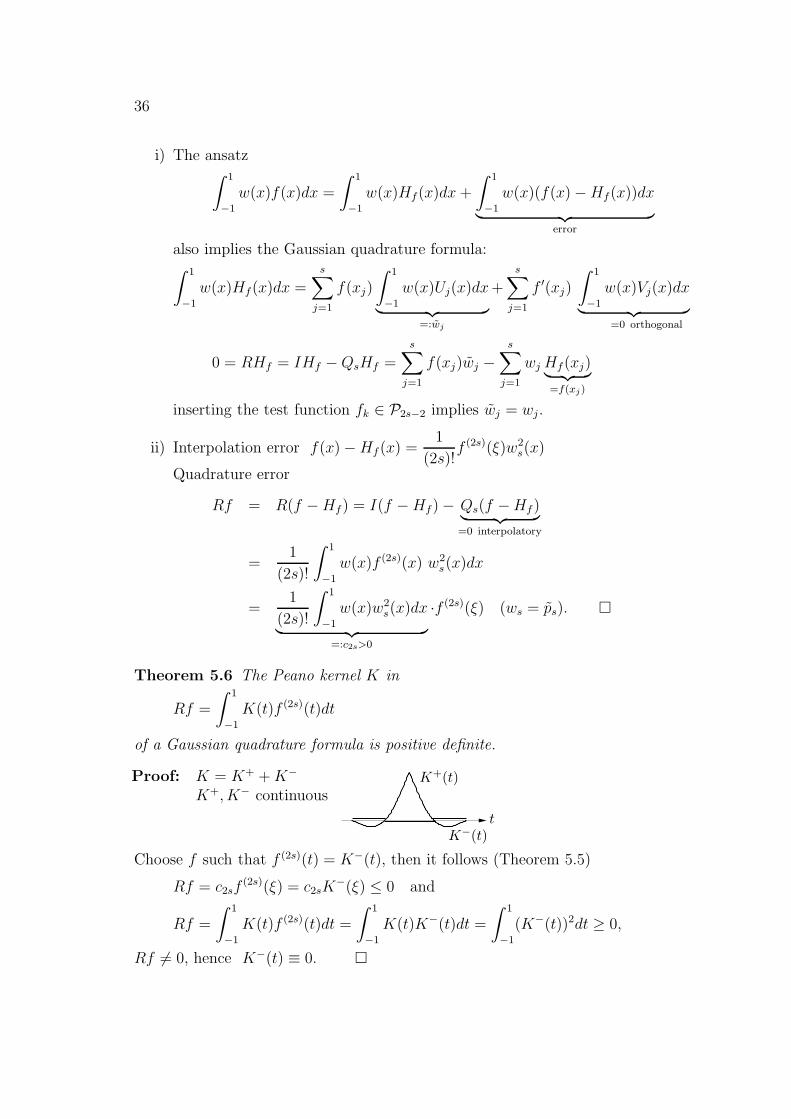
Theorem 5.6 The Peano kernel K in
Rf =
∫ 1
−1
K(t)f (2s)(t)dt
of a Gaussian quadrature formula is positive definite.
Proof: K = K+ +K−
K+, K− continuous
PSfrag replacements K+(t)
K−(t)t
Choose f such that f (2s)(t) = K−(t), then it follows (Theorem 5.5)
Rf = c2sf(2s)(ξ) = c2sK
−(ξ) ≤ 0 and
Rf =
∫ 1
−1
K(t)f (2s)(t)dt =
∫ 1
−1
K(t)K−(t)dt =
∫ 1
−1
(K−(t))2dt ≥ 0,
Rf 6= 0, hence K−(t) ≡ 0. �

5. GAUSSIAN QUADRATURE FORMULAS 37
Theorem 5.7 The Gaussian quadrature formulas are stable.
Proof: Stability → error propagation f(xj) =
{f(xj) + εj, |εj| ≤ εf(xj)(1 + δj), |δj| ≤ δ
the true value Qsf =∑wjf(xj)
perturbed value Qsf =∑wjf(xj)
what is the effect?
Absolute error |Qsf −Qsf | ≤ ‖Qs‖ · ε
Relative error
∣∣∣∣∣Qsf −Qsf
Qsf
∣∣∣∣∣ ≤max |f(xj)||Qsf |︸ ︷︷ ︸natural
· ‖Qs‖︸ ︷︷ ︸numerical
·δ
condition number
Positive weights ‖Qs‖ =
s∑
j=1
|wj| =∫ 1
−1
w(x)dx = µ0
Natural stability
|If − If | ≤ µ0 · ε, ‖I‖ =
∫ 1
−1
ω(x)dx = µ0,
∣∣∣∣∣If − IfIf
∣∣∣∣∣ ≤‖f‖∞|If | µ0 · δ. �
Theorem 5.8 The Gaussian quadrature formula {Qsf}s≥1 is convergent,i.e., lim
s→∞Qsf = If .
Proof
1. {Qs}s≥1 series of bounded functionals (‖Qs‖ ≤ µ0)
2. {Qsf}s≥1 convergent for each algebraic polynomial
Hence, the convergence follows (Theorem of Banach–Steinhaus). �
38
Classical orthogonal polynomials
Jacobian polynomials P(α,β)n
Interval [−1, 1] : w(x) = (1− x)α(1 + x)β, α, β > −1 (singularity ±1)
Special cases
w(x) = 1 : Legendre polynomials Pn(µ0 = 2)
w(x) =1√
1− x2: Tschebyscheff polynomials of the first kind Tn (µ0 = π)
w(x) =√
1− x2 : Tschebyscheff polynomials of the second kind Un (µ0 = π2)
Recurrence formulas
P0(x) = 1, P1(x) = x, (n + 1) Pn+1(x) = (2n+ 1)xPn(x)− nPn−1(x)T0(x) = 1, T1(x) = x, Tn+1(x) = 2xTn(x)− Tn−1(x)U0(x) = 1, U1(x) = 2x, Un+1(x) = 2xUn(x)− Un−1(x)
Infinite intervals (Infinite integrals)
[0,∞) : w(x) = e−x : Laguerre polynomials Ln (µ0 = 1)
L0(x) = 1, L1(x) = −x + 1, Ln+1(x) = (1 + 2n− x)Ln(x)− n2Ln−1(x)
(−∞,∞) : w(x) = e−x2: Hermite polynomials Hn (µ0 =
√π)
H0(x) = 1, H1(x) = 2x, Hn+1(x) = 2xHn(x)− 2nHn−1(x)
Gauss–Legendre
∫ 1
−1
f(x)dx =s∑
j=1
wjf(xj) +Rf
Gauss–Tschebyscheff
∫ 1
−1
1√1− x2
f(x)dx =π
s
s∑
j=1
f(xj) +Rf
All the weights are equal and the nodes xj = cos2j − 1
2sπ, j = 1, . . . , s.
Gauss–Laguerre
∫ ∞
0
e−xf(x)dx =
s∑
j=1
wjf(xj) +Rf
Gauss–Hermite
∫ ∞
∞e−x
2
f(x)dx =s∑
j=1
wjf(xj) +Rf
The main problem: Computation of the nodes and weights
Eigenvalue problem: symmetric tridiagonal matrixthe eigenvalues are the nodes xjthe first coefficient of the normed eigenvectoris equal to the weight wjQR–Algorithm → Method of Golub & van Loan
5. GAUSSIAN QUADRATURE FORMULAS 39
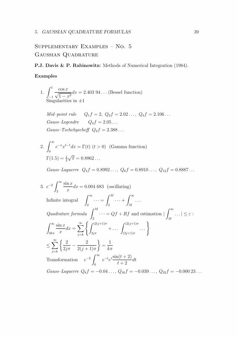
Supplementary Examples – No. 5
Gaussian Quadrature
P.J. Davis & P. Rabinowitz: Methods of Numerical Integration (1984).
Examples
1.
∫ 1
−1
cos x√1− x2
dx = 2.403 94 . . . (Bessel function)
Singularities in ±1
Mid–point rule Q1f = 2, Q2f = 2.02 . . . , Q4f = 2.106 . . .
Gauss–Legendre Q2f = 2.05 . . .
Gauss–Tschebyscheff Q2f = 2.388 . . .
2.
∫ ∞
0
e−xxt−1dx = Γ(t) (t > 0) (Gamma function)
Γ(1.5) = 12
√π = 0.8862 . . .
Gauss–Laguerre Q4f = 0.8992 . . . , Q8f = 0.8910 . . . , Q12f = 0.8887 . . .
3. e−2
∫ ∞
2
sin x
xdx = 0.004 683 (oscillating)
Infinite integral
∫ ∞
2
· · · =∫ M
2
· · ·+∫ ∞
M
. . .
Quadrature formula
∫ M
2
· · · = Qf +Rf and estimation |∫ ∞
M
. . . | ≤ ε :
∫ ∞
2kπ
sin x
xdx =
∞∑
j=k
{∫ (2(j+1)π
2jπ
+ . . .
∫ (2(j+1)π
(2j+1)π
. . .
}
≤∞∑
j=k
{2
2jπ− 2
2(j + 1)π
}=
1
kπ
Transformation e−2
∫ ∞
0
e−tetsin(t+ 2)
t + 2dt
Gauss–Laguerre Q8f = −0.04 . . . , Q16f = −0.039 . . . , Q32f = −0.000 23 . . .
40
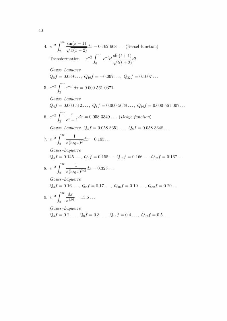
4. e−2
∫ ∞
2
sin(x− 1)√x(x− 2)
dx = 0.162 668 . . . (Bessel function)
Transformation e−2
∫ ∞
0
e−tetsin(t+ 1)√t(t + 2)
dt
Gauss–Laguerre
Q8f = 0.039 . . . , Q16f = −0.097 . . . , Q32f = 0.1007 . . .
5. e−2
∫ ∞
2
e−x2
dx = 0.000 561 0371
Gauss–Laguerre
Q4f = 0.000 512 . . . , Q8f = 0.000 5638 . . . , Q16f = 0.000 561 007 . . .
6. e−2
∫ ∞
2
x
ex − 1dx = 0.058 3349 . . . (Debye function)
Gauss–Laguerre Q4f = 0.058 3351 . . . , Q8f = 0.058 3348 . . .
7. e−2
∫ ∞
2
1
x(log x)2dx = 0.195 . . .
Gauss–Laguerre
Q4f = 0.145 . . . , Q8f = 0.155 . . . Q16f = 0.166 . . . , Q32f = 0.167 . . .
8. e−2
∫ ∞
2
1
x(log x)3/2dx = 0.325 . . .
Gauss–Laguerre
Q4f = 0.16 . . . , Q8f = 0.17 . . . , Q16f = 0.19 . . . , Q32f = 0.20 . . .
9. e−2
∫ ∞
2
dx
x1,01= 13.6 . . .
Gauss–Laguerre
Q4f = 0.2 . . . , Q8f = 0.3 . . . , Q16f = 0.4 . . . , Q32f = 0.5 . . .
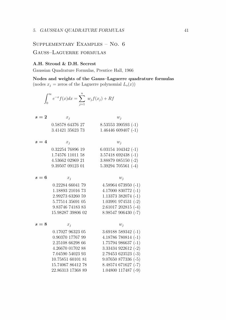
5. GAUSSIAN QUADRATURE FORMULAS 41
Supplementary Examples – No. 6
Gauss–Laguerre formulas
A.H. Stroud & D.H. Secrest
Gaussian Quadrature Formulas, Prentice Hall, 1966
Nodes and weights of the Gauss–Laguerre quadrature formulas(nodes xj = zeros of the Laguerre polynomial Ls(x))
∫ ∞
0
e−xf(x)dx =n∑
j=1
wjf(xj) +Rf
s = 2 xj wj
0.58578 64376 27 8.53553 390593 (-1)3.41421 35623 73 1.46446 609407 (-1)
s = 4 xj wj
0.32254 76896 19 6.03154 104342 (-1)1.74576 11011 58 3.57418 692438 (-1)4.53662 02969 21 3.88879 085150 (-2)9.39507 09123 01 5.39294 705561 (-4)
s = 6 xj wj
0.22284 66041 79 4.58964 673950 (-1)1.18893 21016 73 4.17000 830772 (-1)2.99273 63260 59 1.13373 382074 (-1)5.77514 35691 05 1.03991 974531 (-2)9.83746 74183 83 2.61017 202815 (-4)15.98287 39806 02 8.98547 906430 (-7)
s = 8 xj wj
0.17027 96323 05 3.69188 589342 (-1)0.90370 17767 99 4.18786 780814 (-1)2.25108 66298 66 1.75794 986637 (-1)4.26670 01702 88 3.33434 922612 (-2)7.04590 54023 93 2.79453 623523 (-3)10.75851 60101 81 9.07650 877336 (-5)15.74067 86412 78 8.48574 671627 (-7)22.86313 17368 89 1.04800 117487 (-9)
42
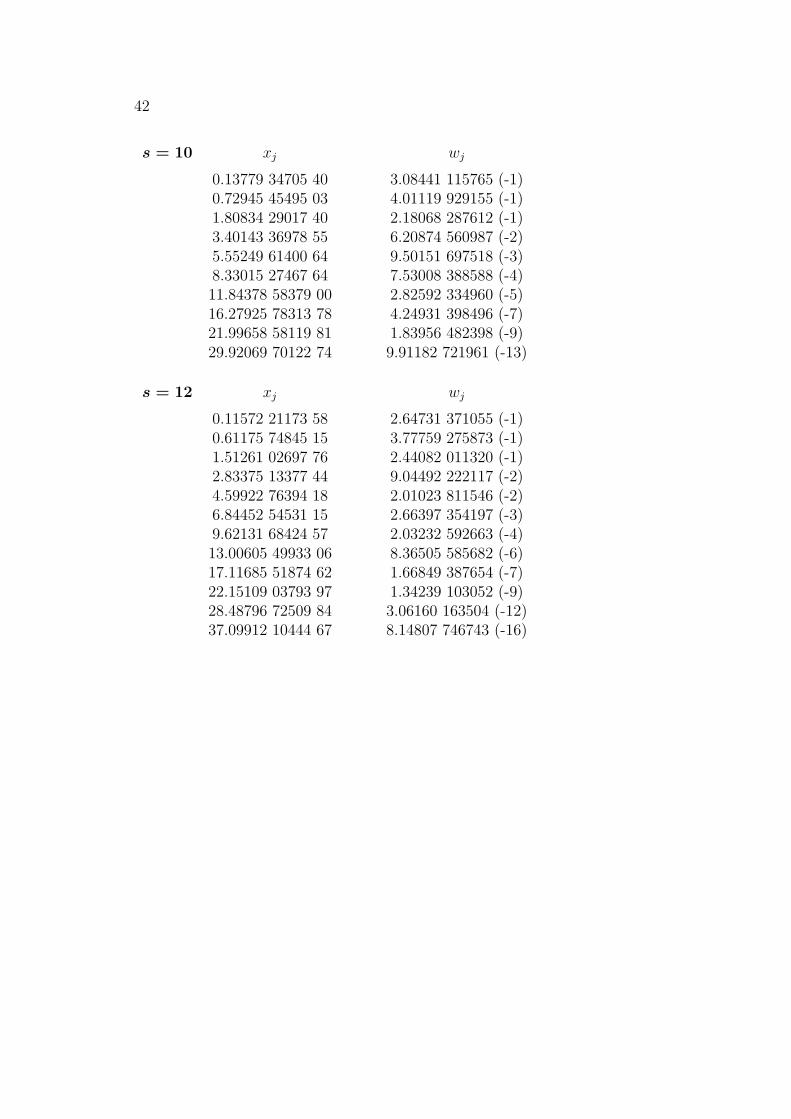
s = 10 xj wj
0.13779 34705 40 3.08441 115765 (-1)0.72945 45495 03 4.01119 929155 (-1)1.80834 29017 40 2.18068 287612 (-1)3.40143 36978 55 6.20874 560987 (-2)5.55249 61400 64 9.50151 697518 (-3)8.33015 27467 64 7.53008 388588 (-4)11.84378 58379 00 2.82592 334960 (-5)16.27925 78313 78 4.24931 398496 (-7)21.99658 58119 81 1.83956 482398 (-9)29.92069 70122 74 9.91182 721961 (-13)
s = 12 xj wj
0.11572 21173 58 2.64731 371055 (-1)0.61175 74845 15 3.77759 275873 (-1)1.51261 02697 76 2.44082 011320 (-1)2.83375 13377 44 9.04492 222117 (-2)4.59922 76394 18 2.01023 811546 (-2)6.84452 54531 15 2.66397 354197 (-3)9.62131 68424 57 2.03232 592663 (-4)13.00605 49933 06 8.36505 585682 (-6)17.11685 51874 62 1.66849 387654 (-7)22.15109 03793 97 1.34239 103052 (-9)28.48796 72509 84 3.06160 163504 (-12)37.09912 10444 67 8.14807 746743 (-16)

6. EXTRAPOLATION METHODS 43
6 Extrapolation Methods
Principle: Richardson extrapolation h→ 0
Application: Discretization (quadrature, numerical differentiation,differential equations)
Example: Numerical differentiation
f ′(0)︸ ︷︷ ︸=:L
=f(h)− f(0)
h︸ ︷︷ ︸=:L(h)
+Rf (h > 0) (difference quotient)
The smaller the step size h becomes the better is the approximation (consistency):L− L(h) = O(h) (h→ 0), L = L(0)
In applications h cannot become arbitrarily small(rounding errors, computational costs)!Better approximation by combination of the values L(h0) und L(h1) with h0, h1.
Error: Asymptotic evaluation (in powers of h)
h0 := h : L− L(h) = − h2!f ′′0 − h2
3!f ′′′0 − . . . = O(h) (h→ 0)| · −1
h1 := h2
: L− L(h2) = − h
2·2!f ′′0 − h2
4·3!f ′′′0 − . . . = O(h) (h→ 0)| · 2
}⇒
L− {2L(h
2)− L(h)
︸ ︷︷ ︸=:L(h)
} = h2
12f ′′′0 + . . . . . . · · · = O(h2) (h→ 0)
Approximation order for L(h) is higher than for L(h)
New formula (difference)
f ′(0) =1
h{−f(h) + 4f(
h
2)− 3f(0)}
︸ ︷︷ ︸=L(h)
+O(h2) (h→ 0)
Acceleration of convergence: step size series h0 > h1 > h2 > . . .
L(h0)
〉 L(h0)
L(h1) 〉 ˜L(h0)
〉 L(h1)
L(h2)...
. . ....
...˜L(h) := 1
3{22L(h
2)− L(h)} = 1
3h{f(h)− 12f(h
2) + 32f(h
4)− 21f(0)}
Order of approximation for ˜L(h) is O(h3) (h→ 0)
44
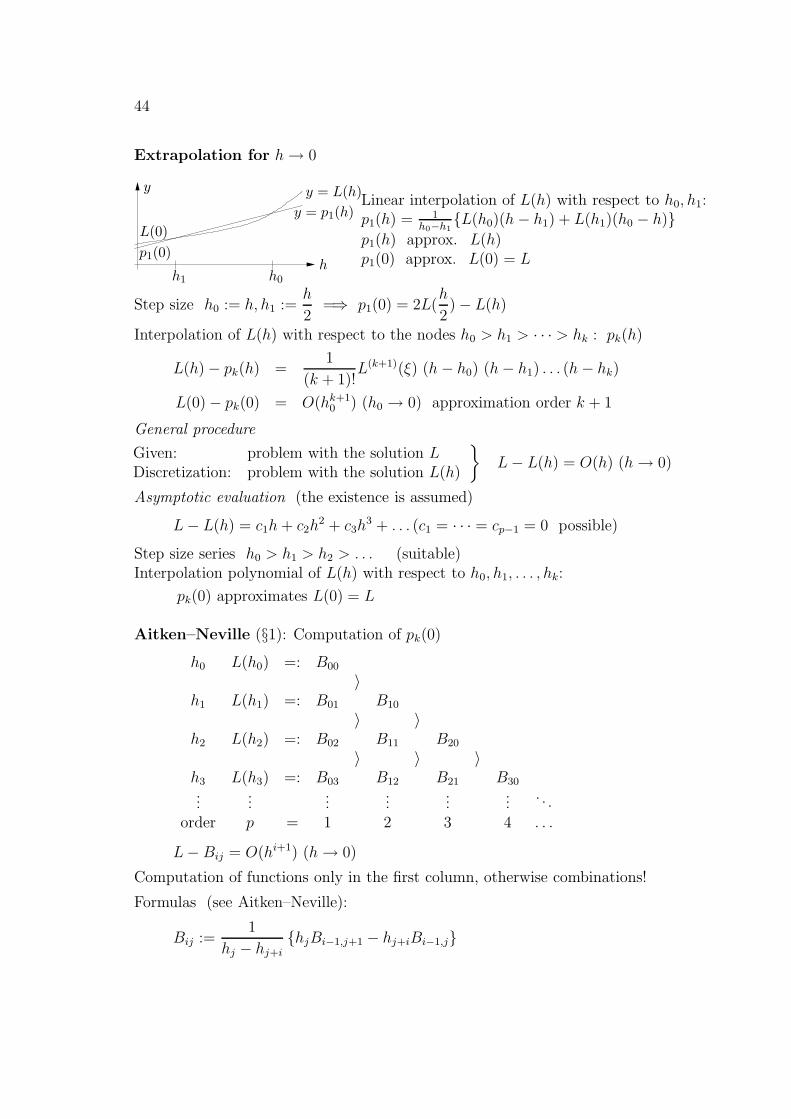
Extrapolation for h→ 0
PSfrag replacements
h1 h0
hp1(0)
L(0)
y = p1(h)
y = L(h)yLinear interpolation of L(h) with respect to h0, h1:p1(h) = 1
h0−h1{L(h0)(h− h1) + L(h1)(h0 − h)}
p1(h) approx. L(h)p1(0) approx. L(0) = L
Step size h0 := h, h1 :=h
2=⇒ p1(0) = 2L(
h
2)− L(h)
Interpolation of L(h) with respect to the nodes h0 > h1 > · · · > hk : pk(h)
L(h)− pk(h) =1
(k + 1)!L(k+1)(ξ) (h− h0) (h− h1) . . . (h− hk)
L(0)− pk(0) = O(hk+10 ) (h0 → 0) approximation order k + 1
General procedure
Given: problem with the solution LDiscretization: problem with the solution L(h)
}L− L(h) = O(h) (h→ 0)
Asymptotic evaluation (the existence is assumed)
L− L(h) = c1h+ c2h2 + c3h
3 + . . . (c1 = · · · = cp−1 = 0 possible)
Step size series h0 > h1 > h2 > . . . (suitable)Interpolation polynomial of L(h) with respect to h0, h1, . . . , hk:
pk(0) approximates L(0) = L
Aitken–Neville (§1): Computation of pk(0)
h0 L(h0) =: B00
〉h1 L(h1) =: B01 B10
〉 〉h2 L(h2) =: B02 B11 B20
〉 〉 〉h3 L(h3) =: B03 B12 B21 B30...
......
......
.... . .
order p = 1 2 3 4 . . .
L− Bij = O(hi+1) (h→ 0)
Computation of functions only in the first column, otherwise combinations!
Formulas (see Aitken–Neville):
Bij :=1
hj − hj+i{hjBi−1,j+1 − hj+iBi−1,j}
6. EXTRAPOLATION METHODS 45
Bisection of the step size hj+1 :=1
2hj, j = 0, 1, 2, · · · :
B1j := 2B0,j+1 − B0,j
B2j :=4B1,j+1 − B1,j
3...
special case B2ν,j :=4νB2ν−1,j+1 −B2ν−1,j
4ν − 1→ Romberg method
Convergence: in columns linear, in diagonals superlinear
Effectivity: Suitable choice of the step size series (to save computations)Special asymptotic evaluations (e.g., in powers of h2)
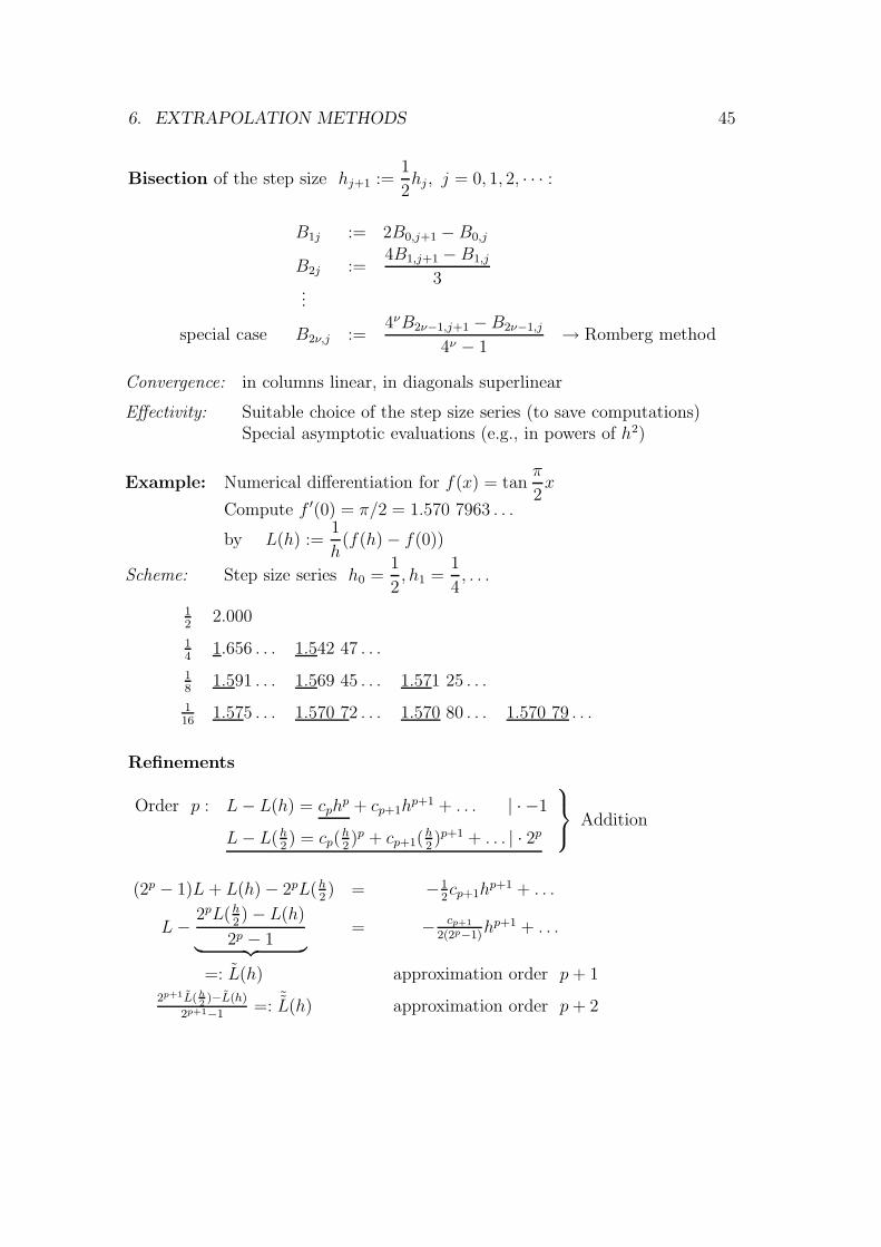
Example: Numerical differentiation for f(x) = tanπ
2x
Compute f ′(0) = π/2 = 1.570 7963 . . .
by L(h) :=1
h(f(h)− f(0))
Scheme: Step size series h0 =1
2, h1 =
1
4, . . .
12
2.000
14
1.656 . . . 1.542 47 . . .
18
1.591 . . . 1.569 45 . . . 1.571 25 . . .
116
1.575 . . . 1.570 72 . . . 1.570 80 . . . 1.570 79 . . .
Refinements
Order p : L− L(h) = cphp + cp+1h
p+1 + . . . | · −1
L− L(h2) = cp(
h2)p + cp+1(h
2)p+1 + . . . | · 2p
Addition
(2p − 1)L + L(h)− 2pL(h2) = −1
2cp+1h
p+1 + . . .
L− 2pL(h2)− L(h)
2p − 1︸ ︷︷ ︸= − cp+1
2(2p−1)hp+1 + . . .
=: L(h) approximation order p+ 12p+1L(h
2)−L(h)
2p+1−1=: ˜L(h) approximation order p+ 2
46
Error estimation
Leading term of the error cphp : subtract the second row from the first row
L(h
2)− L(h) = (1− 1
2p)cph
p +O(hp+1) (h→ 0)
cphp =
L(h2)− L(h)
1− 12p
+O(hp+1) (h→ 0)
cp(h
2)p =
L(h2)− L(h)
2p − 1+O(hp+1) (h→ 0)
Useful for step size control solving differential equations and forthe Romberg method.
Special evaluations
L− L(h) = c2h2 + c4h
4 + c6h6 + . . . (h→ 0) (see trapezoidal rule)
In each extrapolation step the order will be increased by two.
Romberg method “Automatic integration” (Numer. Math. I)
Compute an approximation N for I :=
∫ b
a
f(x)dx with |N − I| ≤ ε
Trapezoidal sum (n subintervals of length h = b−an
)
∫ b
a
f(x)dx = hn∑
ν=0
′′f(a+ νh)
︸ ︷︷ ︸=:T (h)
+Rf (Σ′′ : first and last term are cut in halves)
Convergence T (h)→ I = T (0) for h→ 0
Error (Numer. Math. I): Rf = −(b− a)3
12
1
n2f ′′(ξ) = O(h2) (h→ 0)
Asymptotic evaluation (f sufficiently smooth)
I − T (h) = c2h2 + c4h
4 + . . . (h→ 0), (powers in h2)
Romberg series h0, h1, h2, . . . , hν := h0
2ν, h0 = b− a (bisection)
Combinations
T (h) :=4T (h
2)−T (h)
3Kepler Σ, degree of exactness 3
˜T (h) :=42T (h
2)−T (h)
42−1Boole Σ, degree of exactness 5
...
6. EXTRAPOLATION METHODS 47
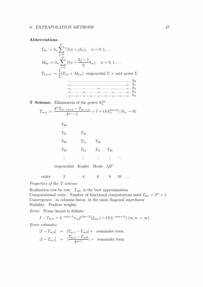
Abbreviations
T0n := hn
2n∑
j=0
′′f(a+ jhn), n = 0, 1, . . .
M0n := hn
2n∑
j=1
f(a+2j − 1
2hn), n = 0, 1, . . .
T0,n+1 :=1
2(T0,n +M0,n) trapezoidal Σ + mid–point Σ
PSfrag replacements
h0h1h2h3h4
T–Scheme: Elimination of the power h2mn
Tm,n :=4mTm−1,n+1 − Tm−1,n
4m − 1= I +O(h2m+2
n ) (hn → 0)
T00
T01 T10
T02 T11 T20
T03 T12 T21 T30
......
......
. . .
trapezoidal Kepler Boole QF
order 2 4 6 8 10 . . .
Properties of the T–scheme
Realization row by row: Tm0 is the best approximationComputational costs: Number of functional computations until T0m = 2m + 1Convergence: in columns linear, in the main diagonal superlinearStability: Positive weights
Error: Peano kernel is definite
I − Tm,n = 4−n(m+1)cmf(2m+2)(ξmn) = O(4−n(m+1)) (m,n→∞)
Error estimates
|I − Tm,0| = |Tm,1 − Tm,0|+ remainder term
|I − Tm,1| = |Tm,1 − Tm,04m+1
|+ remainder term
48
Stopping criterion (fast convergence!)
|Tm,1 − Tm,0| · dm ≤ ε =⇒ |If − Tm+1,0| ≤ εdm damping factor, e.g. dm = 4−m−1
Example:
∫ 2
1
dx
x= ln 2 = 0.693 147 180 . . .
0.750.708 . . . 0.694 . . .0.697 . . . 0.693 25 . . . 0.693 17 . . .0.694 . . . 0.693 15 . . . 0.693 148 . . . 0.693 147 47 . . .
|T21 − T20| = 3 · 10−5, d2|T21 − T20| = 4.7 · 10−7,|I − T20| = 3 · 10−5, |I − T21| = 1 · 10−6, |I − T30| = 3 · 10−7
Asymptotic evaluation for the trapezoidal sum
Theorem 6.1 (Formula of Euler–MacLaurin)Let f ∈ C2k+1[0, 1], then it holds
12[f(0) + f(1)] =
∫ 1
0f(x)dx+ b2
2![f ′(1)− f ′(0)] + b4
4![f ′′′(1)− f ′′′(0)] + . . .
· · ·+ b2k(2k)!
[f (2k−1)(1)− f (2k−1)(0)] +R2k+1f, where
R2k+1f =∫ 1
0B2k+1(x)f (2k+1)(x)dx,
Bn(x) Bernoulli polynomials,
bn := Bn(0)n! Bernoulli numbers.
Remark: Euler–MacLaurin f(0), f(1), f ′(0), f ′(1), f ′′′(0), f ′′′(1)
Taylor evaluation f(0), f ′(0), f ′′(0), . . . ,
Bernoulli polynomials
B0(x) := 1
Bn+1(x) :=∫Bn(x)dx with a constant such that
∫ 1
0Bn+1(x)dx = 0
B1(x) = x− 12
B2(x) = 12x2 − 1
2x+ 1
12
B3(x) = 16x3 − 1
4x2 + 1
12x
B4(x) = 124x4 − 1
12x3 + 1
24x2 − 1
720...
Leading coefficient of Bn : 1n!
6. EXTRAPOLATION METHODS 49
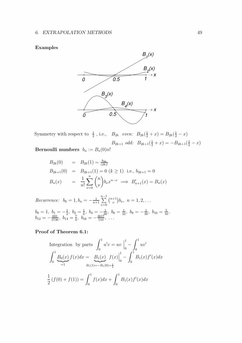
Examples
0
0
0.5
0.5
1
1
x
x
B1(x)
B2(x)
B3(x)
B4(x)
Symmetry with respect to 12
, i.e., B2k even: B2k(12
+ x) = B2k(12− x)
B2k+1 odd: B2k+1(12
+ x) = −B2k+1(12− x)
Bernoulli numbers bn := Bn(0)n!
B2k(0) = B2k(1) = b2k(2k)!
B2k+1(0) = B2k+1(1) = 0 (k ≥ 1) i.e., b2k+1 = 0
Bn(x) =1
n!
n∑
ν=0
(n
ν
)bνx
n−ν =⇒ B′n+1(x) = Bn(x)
Recurrence: b0 = 1, bn = − 1n+1
n−1∑ν=0
(n+1ν
)bν, n = 1, 2, . . .
b0 = 1, b1 = −12, b2 = 1
6, b4 = − 1
30, b6 = 1
42, b8 = − 1
30, b10 = 5
16,
b12 = − 6912730
, b14 = 76, b16 = −3617
510, . . .
Proof of Theorem 6.1:
Integration by parts
∫ 1
0
u′v = uv∣∣∣1
0−∫ 1
0
uv′
∫ 1
0
B0(x)︸ ︷︷ ︸=1
f(x)dx = B1(x)︸ ︷︷ ︸B1(1)=−B1(0)= 1
2
f(x)∣∣∣1
0−∫ 1
0
B1(x)f ′(x)dx
1
2(f(0) + f(1)) =
∫ 1
0
f(x)dx+
∫ 1
0
B1(x)f ′(x)dx
50
∫ 1
0
B1(x)f ′(x)dx =B2(x)︸ ︷︷ ︸B2(1)=B2(0)=
b22!
f ′(x)dx∣∣∣1
0−∫ 1
0
B2(x)f ′′(x)dx
=b2
2![f ′(1)− f ′(0)]−
∫ 1
0
B2(x)f ′′(x)dx
−∫ 1
0
B2(x)f ′′(x)dx = − B3(x)︸ ︷︷ ︸B3(1)=B3(0)=0
f ′′(x)
∫ 1
0
+
∫ 1
0
B3(x)f ′′′(x)dx
= B4(x)︸ ︷︷ ︸B4(1)=B4(0)=
b44!
f ′′′(x)−∫ 1
0
B4(x)f (4)(x)dx
=b4
4![f ′′′(1)− f ′′′(0)]−
∫ 1
0
B4(x)f (4)(x)dx
In general (` ≥ 1)
−∫ 1
0
B2`(x)f (2`)(x)dx =
∫ 1
0
B2`+1(x)f (2`+1)(x)dx∫ 1
0
B2`+1(x)f (2`+1)(x)dx =b2`+2
(2`+ 2)!
[f (2`+1)(1)− f (2`+1)(0)
]
−∫ 1
0
B2`+2(x)f (2`+2)(x)dx �
Trapezoidal Σ: Subintervals [0, 1], [1, 2], . . . , [n− 1, n]→ compensation of derivatives
n∑
j=0
′′f(j) =
∫ n
0
f(x)dx+k∑
j=1
b2j
(2j)!
[f (2j−1)(n)− f (2j−1)(0)
]
+
∫ n
0
B∗2k+1(x)f (2k+1)(x)dx
B∗2k+1(x) by periodic continuation of B2k+1(x) in [0, 1)
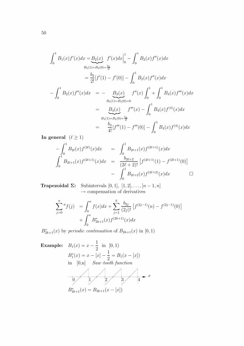
Example: B1(x) = x− 1
2in [0, 1)
B∗1(x) = x− [x]− 1
2= B1(x− [x])
in [0,n] Saw–tooth functionPSfrag replacements
0 1 2 3 4x
B∗2k+1(x) = B2k+1(x− [x])
6. EXTRAPOLATION METHODS 51
Theorem 6.2 Let f ∈ C2k+1[a, b], then the asymptotic evaluation holds
Tf(h) =
∫ b
a
f(x)dx +k∑
j=1
b2j
(2j)!
[f (2j−1)(b)− f (2j−1)(a)
]h2j + h2k+1R∗2k+1f.
Remark: Evaluation in powers of h2
Proof: Transform [0, n]→ [a, b] with grid length h =b− an
x 7→ t = a+ xh, dt = h dx
f(x) = f(t−ah
)=: f(t), f (ν)(x) = hν f (ν)(t)
1
hTf(h)︸ ︷︷ ︸
=hΣ′′f(a+jh)
=1
h
∫ b
a
f(t)dt +k∑
j=1
b2j
(2j)!h2j−1[f (2j−1)(b)− f (2j−1)(a)]
+h2k+1
h
b∫
a
B∗2k+1(t)f (2k+1)(t)dt
︸ ︷︷ ︸=:R∗2k+1f
�
Periodic function f ∈ C2k+1[a,b] , i.e.,
f ′(a) = f ′(b), . . . , f (2k−1)(a) = f (2k−1)(b)
Corollary 6.3 Let f ∈ C2k+1[a,b] , then the error of the trapezoidal rule satisfies
∫ b
a
f(x)dx− T (h) = O(h2k+1) (h→ 0).
Remarks: The trapezoidal rule is the best possible approximation,but the integrand f does not always satisfy the smoothness.T (h) is used for the computation of Fourier coefficients.
52
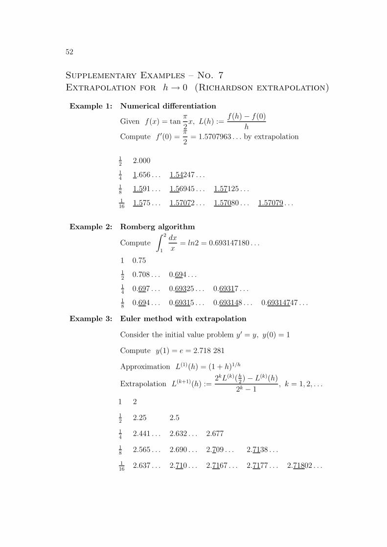
Supplementary Examples – No. 7
Extrapolation for h→ 0 (Richardson extrapolation)
Example 1: Numerical differentiation
Given f(x) = tanπ
2x, L(h) :=
f(h)− f(0)
h
Compute f ′(0) =π
2= 1.5707963 . . . by extrapolation
12
2.000
14
1.656 . . . 1.54247 . . .
18
1.591 . . . 1.56945 . . . 1.57125 . . .
116
1.575 . . . 1.57072 . . . 1.57080 . . . 1.57079 . . .
Example 2: Romberg algorithm
Compute
∫ 2
1
dx
x= ln2 = 0.693147180 . . .
1 0.75
12
0.708 . . . 0.694 . . .
14
0.697 . . . 0.69325 . . . 0.69317 . . .
18
0.694 . . . 0.69315 . . . 0.693148 . . . 0.69314747 . . .
Example 3: Euler method with extrapolation
Consider the initial value problem y′ = y, y(0) = 1
Compute y(1) = e = 2.718 281
Approximation L(1)(h) = (1 + h)1/h
Extrapolation L(k+1)(h) :=2kL(k)(h
2)− L(k)(h)
2k − 1, k = 1, 2, . . .
1 2
12
2.25 2.5
14
2.441 . . . 2.632 . . . 2.677
18
2.565 . . . 2.690 . . . 2.709 . . . 2.7138 . . .
116
2.637 . . . 2.710 . . . 2.7167 . . . 2.7177 . . . 2.71802 . . .
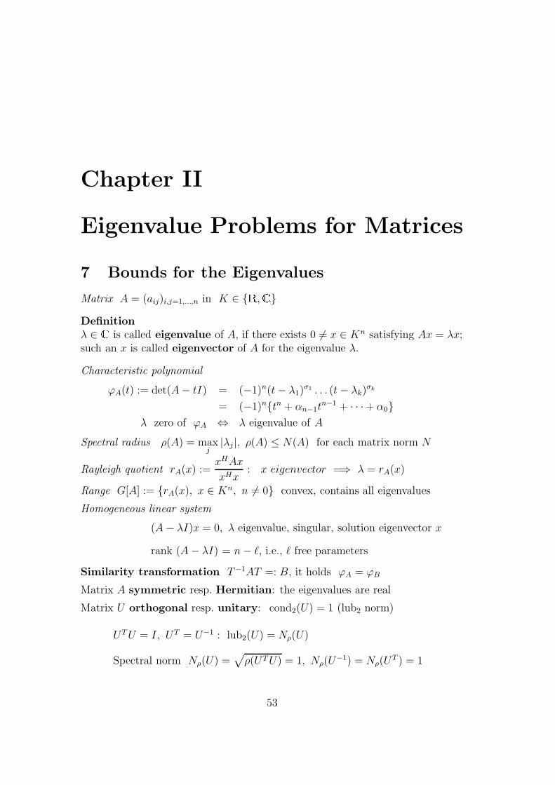
Chapter II
Eigenvalue Problems for Matrices
7 Bounds for the Eigenvalues
Matrix A = (aij)i,j=1,...,n in K ∈ { �, � }
Definitionλ ∈ � is called eigenvalue of A, if there exists 0 6= x ∈ Kn satisfying Ax = λx;such an x is called eigenvector of A for the eigenvalue λ.
Characteristic polynomial
ϕA(t) := det(A− tI) = (−1)n(t− λ1)σ1 . . . (t− λk)σk= (−1)n{tn + αn−1t
n−1 + · · ·+ α0}λ zero of ϕA ⇔ λ eigenvalue of A
Spectral radius ρ(A) = maxj|λj|, ρ(A) ≤ N(A) for each matrix norm N
Rayleigh quotient rA(x) :=xHAx
xHx: x eigenvector =⇒ λ = rA(x)
Range G[A] := {rA(x), x ∈ Kn, n 6= 0} convex, contains all eigenvalues
Homogeneous linear system
(A− λI)x = 0, λ eigenvalue, singular, solution eigenvector x
rank (A− λI) = n− `, i.e., ` free parameters
Similarity transformation T−1AT =: B, it holds ϕA = ϕB
Matrix A symmetric resp. Hermitian: the eigenvalues are real
Matrix U orthogonal resp. unitary: cond2(U) = 1 (lub2 norm)
UTU = I, UT = U−1 : lub2(U) = Nρ(U)
Spectral norm Nρ(U) =√ρ(UTU) = 1, Nρ(U
−1) = Nρ(UT ) = 1
53
54
Real matrix A positive definite
A symmetric and xTAx > 0 f.a. 0 6= x ∈ � n ⇔ the eigenvalues are positive
Matrix A normal: AHA = AAH (⇔ unitarily similar to a diagonal matrix)
→ Important theorems (see Stoer & Bulirsch)
Theorem 7.1 (Theorem of Schur)For each A ∈ Kn×n exists an unitary U with
UHAU =
λ1 ∗. . .
0 λn
.
Theorem 7.2 Each Hermitian A is unitarily similar to a diagonal matrix,i.e., UHAU = diag(λ1, . . . , λn) with unitary U = (u1, . . . , un).The j–th column vector uj is eigenvector of the eigenvalue λj : Auj = λjuj.Hence A has n linearily independent eigenvectors which are orthogonal.
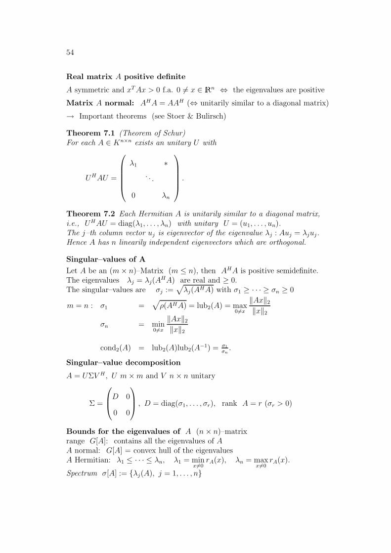
Singular–values of A
Let A be an (m× n)–Matrix (m ≤ n), then AHA is positive semidefinite.The eigenvalues λj = λj(A
HA) are real and ≥ 0.The singular–values are σj :=
√λj(AHA) with σ1 ≥ · · · ≥ σn ≥ 0
m = n : σ1 =√ρ(AHA) = lub2(A) = max
06=x
‖Ax‖2
‖x‖2
σn = min06=x
‖Ax‖2
‖x‖2
cond2(A) = lub2(A)lub2(A−1) = σ1
σn.
Singular–value decomposition
A = UΣV H , U m×m and V n× n unitary
Σ =
D 0
0 0
, D = diag(σ1, . . . , σr), rank A = r (σr > 0)
Bounds for the eigenvalues of A (n× n)–matrixrange G[A]: contains all the eigenvalues of AA normal: G[A] = convex hull of the eigenvaluesA Hermitian: λ1 ≤ · · · ≤ λn, λ1 = min
x6=0rA(x), λn = max
x6=0rA(x).
Spectrum σ[A] := {λj(A), j = 1, . . . , n}
7. BOUNDS FOR THE EIGENVALUES 55
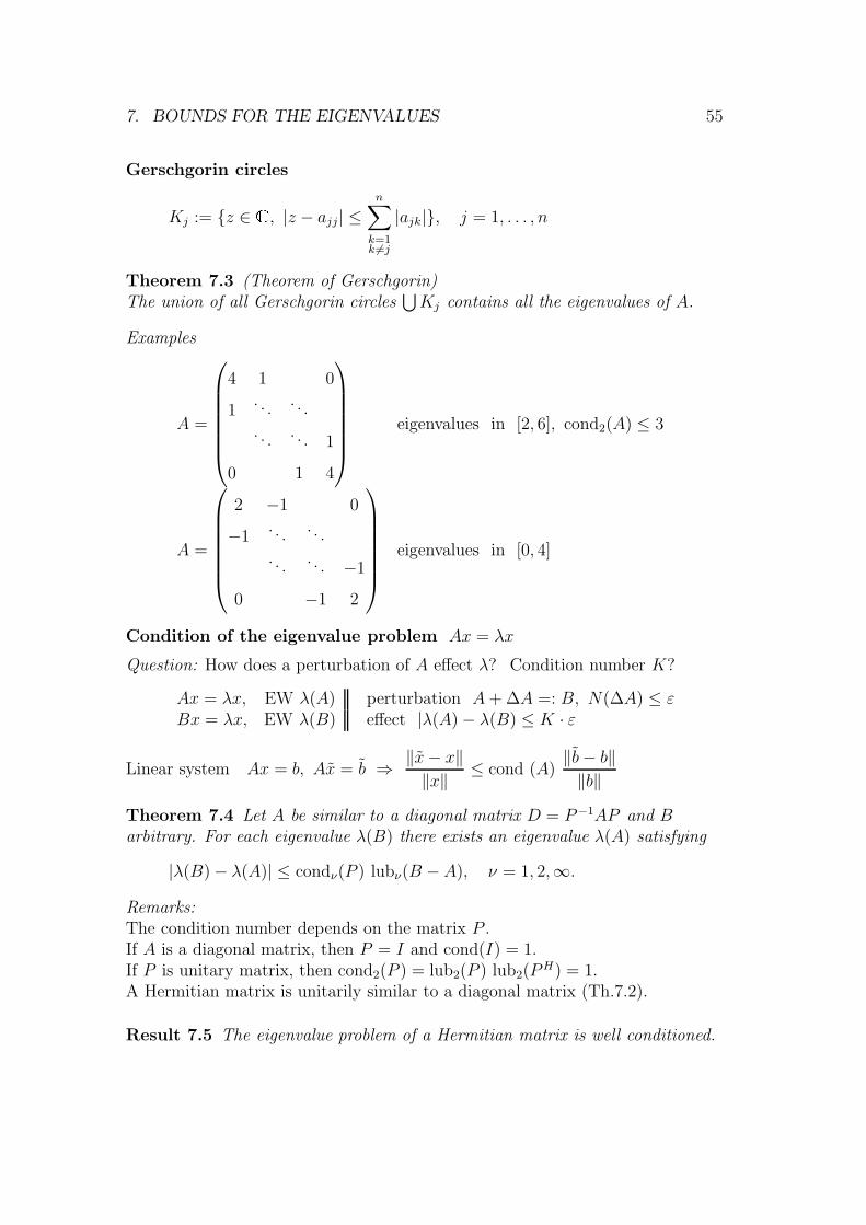
Gerschgorin circles
Kj := {z ∈ � , |z − ajj| ≤n∑
k=1k 6=j
|ajk|}, j = 1, . . . , n
Theorem 7.3 (Theorem of Gerschgorin)The union of all Gerschgorin circles
⋃Kj contains all the eigenvalues of A.
Examples
A =
4 1 0
1. . .
. . .
. . .. . . 1
0 1 4
eigenvalues in [2, 6], cond2(A) ≤ 3
A =
2 −1 0
−1. . .
. . .
. . .. . . −1
0 −1 2
eigenvalues in [0, 4]
Condition of the eigenvalue problem Ax = λx
Question: How does a perturbation of A effect λ? Condition number K?
Ax = λx, EW λ(A) perturbation A+ ∆A =: B, N(∆A) ≤ εBx = λx, EW λ(B) effect |λ(A)− λ(B) ≤ K · ε
Linear system Ax = b, Ax = b ⇒ ‖x− x‖‖x‖ ≤ cond (A)
‖b− b‖‖b‖
Theorem 7.4 Let A be similar to a diagonal matrix D = P−1AP and Barbitrary. For each eigenvalue λ(B) there exists an eigenvalue λ(A) satisfying
|λ(B)− λ(A)| ≤ condν(P ) lubν(B − A), ν = 1, 2,∞.
Remarks:The condition number depends on the matrix P .If A is a diagonal matrix, then P = I and cond(I) = 1.If P is unitary matrix, then cond2(P ) = lub2(P ) lub2(PH) = 1.A Hermitian matrix is unitarily similar to a diagonal matrix (Th.7.2).
Result 7.5 The eigenvalue problem of a Hermitian matrix is well conditioned.

56
Corollary 7.6 Let λ be an eigenvalue of B, but not of A, then it holds
1 ≤ lub((λI − A)−1(B − A)
)≤ lub
((λI − A)−1
)lub (B − A).
Proof: (B − A)x = (λI − A)x =⇒ (λI − A)−1
︸ ︷︷ ︸=:H
(B − A)︸ ︷︷ ︸=:G
x = x
x = H ·Gx : ‖x‖ = ‖HGx‖ ≤ N(HG)‖x‖ ≤ N(H)N(G)‖x‖. �
Corollary 7.6 implies the proof of Theorem 7.3 (Gerschgorin)for the matrix B:
B = (bij), A := diag(b11, . . . , bnn)
1 ≤ lub∞ ((λI − A)−1(B − A)) ≤ max1≤j≤n
1
|λ− bjj|n∑
k=1k 6=j
|bjk| �
Proof of Theorem 7.4:
AssumptionsA = PDP−1, D = diag(λ1(A), . . . , λn(A)λ = λ(B) eigenvalue of B, but not of A (else the statement is trivial)(λI − A)−1 = P (λI −D)−1P−1
λ 6= λj(A) for all j : estimation of minj|λ− λj(A)|
λ− λj(A) is eigenvalue of λI −D1
λ− λj(A)is eigenvalue of (λI −D)−1
maxj1
|λ−λj(A)| = lubν ((λI −D)−1
︸ ︷︷ ︸), ν = 1, 2,∞
↑ diagonal matrix
does not hold
for all norms
lub ((λI − A)−1) ≤ lub(P ) lub ((λI −D)−1) lub(P−1)= cond(P ) lub ((λI −D)−1)
Corollary 7.6 ⇒ 1 ≤ condν(P ) maxj1
|λ−λj(A)| lubν(B − A)
hence minj|λ− λj(A)| ≤ condν(P ) lubν(B − A). �
Similar matrices by suitable transformations
Given: eigenvalue problem Ax = λx with condition number cond(P )Wanted: equivalent problem Ax = λx with an easier matrixby transforming matrix T with A = T−1AT .Question: How does T effect the condition of the eigenvalue problem?
7. BOUNDS FOR THE EIGENVALUES 57
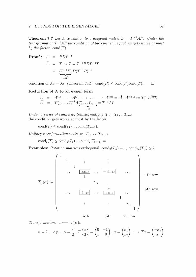
Theorem 7.7 Let A be similar to a diagonal matrix D = P−1AP . Under thetransformation T−1AT the condition of the eigenvalue problem gets worse at mostby the factor cond(T ).
Proof : A = PDP−1
A = T−1AT = T−1PDP−1T
= (T−1P )︸ ︷︷ ︸=:P
D(T−1P )−1
condition of Ax = λx (Theorem 7.4): cond(P ) ≤ cond(P )cond(T ). �
Reduction of A to an easier form
A =: A(1) −→ A(2) −→ . . . −→ A(m) =: A, A(i+1) := T−1i A(i)Ti
A = T−1m−1 . . . T
−11 AT1 . . . Tm−1︸ ︷︷ ︸
=:T
= T−1AT
Under a series of similarity transformations T := T1 . . . Tm−1
the condition gets worse at most by the factor
cond(T ) ≤ cond(T1) . . . cond(Tm−1).
Unitary transformation matrices T1, . . . , Tm−1:
cond2(T ) ≤ cond2(T1) . . . cond2(Tm−1) = 1
Examples: Rotation matrices orthogonal, cond2(Tij) = 1, cond∞(Tij) ≤ 2
Tij(α) :=
1. . .
......
1
. . . cosα . . . − sinα . . .1
. . .
1
. . . sinα . . . cosα . . .1
......
. . .
1
i-th row
j-th row
i-th j-th column
Transformation: x 7−→ T (α)x
n = 2 : e.g., α =π
2: T(π
2
)=
(0 −11 0
), x =
(x1
x2
)7−→ Tx =
(−x2
x1
)
58PSfrag replacements
−x2 x11st comp.
xx2
2nd comp.
x1Tx
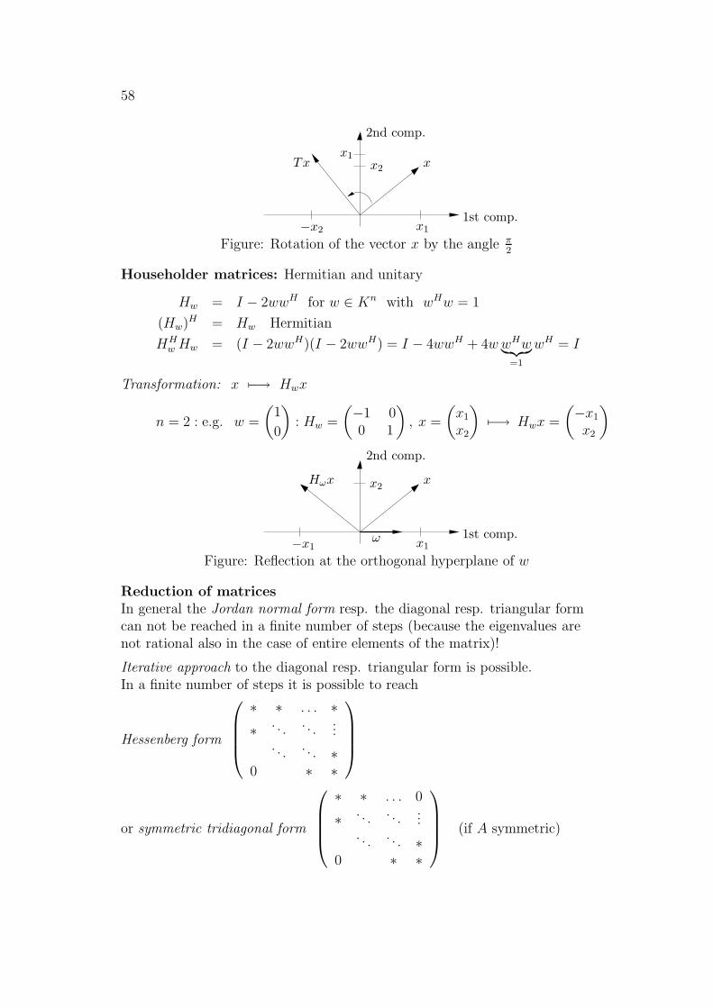
Figure: Rotation of the vector x by the angle π2
Householder matrices: Hermitian and unitary
Hw = I − 2wwH for w ∈ Kn with wHw = 1
(Hw)H = Hw Hermitian
HHwHw = (I − 2wwH)(I − 2wwH) = I − 4wwH + 4wwHw︸ ︷︷ ︸
=1
wH = I
Transformation: x 7−→ Hwx
n = 2 : e.g. w =
(1
0
): Hw =
(−1 00 1
), x =
(x1
x2
)7−→ Hwx =
(−x1
x2
)PSfrag replacements
−x1ω x1
1st comp.
xx2Hωx
2nd comp.
Figure: Reflection at the orthogonal hyperplane of w
Reduction of matricesIn general the Jordan normal form resp. the diagonal resp. triangular formcan not be reached in a finite number of steps (because the eigenvalues arenot rational also in the case of entire elements of the matrix)!
Iterative approach to the diagonal resp. triangular form is possible.In a finite number of steps it is possible to reach
Hessenberg form
∗ ∗ . . . ∗∗ . . .
. . ....
. . .. . . ∗
0 ∗ ∗
or symmetric tridiagonal form
∗ ∗ . . . 0
∗ . . .. . .
.... . .
. . . ∗0 ∗ ∗
(if A symmetric)
7. BOUNDS FOR THE EIGENVALUES 59
Computation of the eigenvalues of a matrix
In principle: evaluation of the characteristic polynomial,then methods for computing zeros ofpolynomials
Direct methods: reduction of the matrix to an easier form,characteristic polynomial by recurrence formulas,then special methods for computing the zeros
Iterative methods: construction of a series of matrices {A(i)}i≥0
by transformations T−1i A(i)Ti
with A(i) →
λ1 ∗
. . .
0 λn
if i→∞
Vector iteration: Raising to a higher power Akx = λkx(“destilling” the largest eigenvalues in absolut value!)
60
8 Eigenvalues of Symmetric Matrices
Real matrix An =
a11 a12
a12 a22. . . 0
. . .. . . an−1,n
0 an−1,n ann
eigenvalues real
An is called irreducible, if aj−1,j 6= 0, j = 2, . . . , n and reducible otherwise.
If An is irreducible, then the eigenvalues are real and simple.
If An is reducible, then reduction of the problem to
A =
(Ak 00 Bn−k
),
i.e., the characteristic polynomial satisfies ϕAn = ϕAk · ϕBn−k .Main matrices
Ak :=
a11 a12
a12. . .
. . . 0. . .
. . . ak−1,k
0 ak−1,k akk
, k = 1, . . . , n
characteristic polynomial ϕk(t) = det(Ak − tI), degree ϕk = k
Theorem 8.1 (3–term recurrence relation)The characteristic polynomial ϕn of a symmetric tridiagonal matrix An
is deduced by the recurrence formula
ϕ0(t) := 1, ϕ1(t) := a11 − tϕk(t) := (akk − t) ϕk−1(t)− a2
k−1,k ϕk−2(t), k = 2, 3, . . . , n.
Proof: Evaluation of the determinant by the last column. �
Theorem 8.2 (Zeros)Let An be an irreducible symmetric tridiagonal matrix.The characteristic polynomial ϕk of Ak (1 ≤ k ≤ n) has k real
and simple zeros λ(k)1 < · · · < λ
(k)k .
The zeros of ϕk+1 are separated by the zeros of ϕk,
i.e., λ(k+1)ν < λ
(k)ν < λ
(k+1)ν+1 for 1 ≤ ν ≤ k.
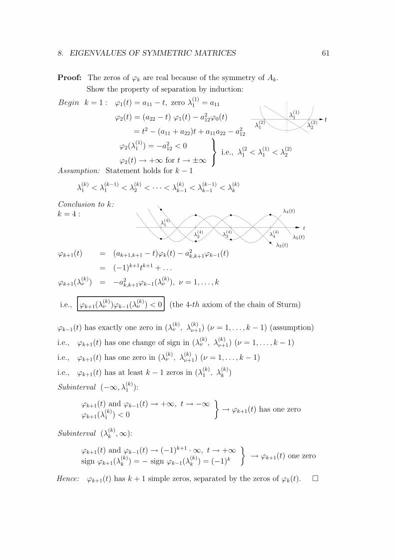
8. EIGENVALUES OF SYMMETRIC MATRICES 61
Proof: The zeros of ϕk are real because of the symmetry of Ak.
Show the property of separation by induction:
Begin k = 1 : ϕ1(t) = a11 − t, zero λ(1)1 = a11
ϕ2(t) = (a22 − t) ϕ1(t)− a212ϕ0(t)
= t2 − (a11 + a22)t + a11a22 − a212
ϕ2(λ(1)1 ) = −a2
12 < 0
ϕ2(t)→ +∞ for t→ ±∞
i.e., λ
(21 < λ
(1)1 < λ
(2)2
PSfrag replacements
λ(2)1
λ(1)1
λ(2)2
t
Assumption: Statement holds for k − 1
λ(k)1 < λ
(k−1)1 < λ
(k)2 < · · · < λ
(k)k−1 < λ
(k−1)k−1 < λ
(k)k
Conclusion to k:k = 4 :
PSfrag replacements
λ(4)1
λ(4)2 λ
(4)3 λ
(4)4
t
λ3(t)
λ5(t)
λ4(t)
ϕk+1(t) = (ak+1,k+1 − t)ϕk(t)− a2k,k+1ϕk−1(t)
= (−1)k+1tk+1 + . . .
ϕk+1(λ(k)ν ) = −a2
k,k+1ϕk−1(λ(k)ν ), ν = 1, . . . , k
i.e., ϕk+1(λ(k)ν )ϕk−1(λ
(k)ν ) < 0 (the 4-th axiom of the chain of Sturm)
ϕk−1(t) has exactly one zero in (λ(k)ν , λ
(k)ν+1) (ν = 1, . . . , k − 1) (assumption)
i.e., ϕk+1(t) has one change of sign in (λ(k)ν , λ
(k)ν+1) (ν = 1, . . . , k − 1)
i.e., ϕk+1(t) has one zero in (λ(k)ν , λ
(k)ν+1) (ν = 1, . . . , k − 1)
i.e., ϕk+1(t) has at least k − 1 zeros in (λ(k)1 , λ
(k)k )
Subinterval (−∞, λ(k)1 ):
ϕk+1(t) and ϕk−1(t)→ +∞, t→ −∞ϕk+1(λ
(k)1 ) < 0
}→ ϕk+1(t) has one zero
Subinterval (λ(k)k ,∞):
ϕk+1(t) and ϕk−1(t)→ (−1)k+1 · ∞, t→ +∞sign ϕk+1(λ
(k)k ) = − sign ϕk−1(λ
(k)k ) = (−1)k
}→ ϕk+1(t) one zero
Hence: ϕk+1(t) has k + 1 simple zeros, separated by the zeros of ϕk(t). �

62
Remark: Compare this result with the zeros of orthogonal polynomials.
Example
0 1√2
0 0
1√2
0 12
0
0 12
0 12
0 0 12
0. . .
. . .. . .
ϕ0(t) = 1, ϕ1(t) = −t, ϕ2(t) = t2 − 12,
ϕ3(t) = −(t3 − 34t), ϕ4(t) = t4 − t2 + 1
8, . . .
→ chain of Sturm
→ Tschebyscheff polynomials (notice the sign)
T0 = 1, T1 = t, T2 = 2t2 − 1, T3 = 4t3 − 3t,
T4 = 8t4 − 8t2 + 1, . . .
Theorem 8.3 (Chain of Sturm)Let An be an irreducible symmetric tridiagonal matrix.The characteristic polynomials ϕk of Ak, k = 1, . . . n (with alternating signs)
(−1)nϕn, (−1)n−1ϕn−1, . . . , (−1)ϕ1, ϕ0
form a chain of Sturm in [α, β] with ϕn(α)ϕn(β) 6= 0.
Proof: Check the axioms of the chain of Sturm (see Numer. Math. I)
(1) ϕn(α)ϕn(β) 6= 0
(2) ϕ0(t) 6= 0
(3) ϕn(t) only simple zeros ξand ϕ′n(ξ)ϕn−1(ξ) < 0
(4) ϕk(η) = 0 then
ϕk+1(η)ϕk−1(η) < 0
PSfrag replacements
λ(4)1
λ(4)2
λ(4)3
λ(4)4 t
ϕ3(t)
ϕ4(t)
Number of sign–changes W (t) := W ((−1)nϕn(t), . . . , ϕ0(t))
Theorem of Sturm (see Numer. Math. I):
The number of zeros in (α, β) satisfies Zβα(ϕn) = W (α)−W (β).
Bisection method: Determine an interval [α, β] of lenght ε withat least (or exactly) one zero
Newton method with a suitable initial value
Derivative by recurrence ϕ′0(t) = 0, ϕ′1(t) = −1
ϕ′k(t) = −ϕk−1(t) + (akk − t)ϕ′k−1(t)− a2k−1,kϕ
′k−2(t)
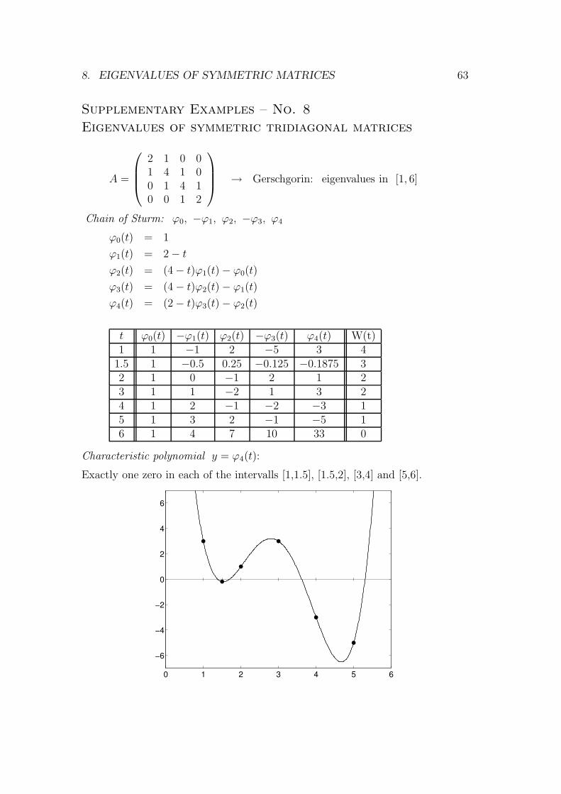
8. EIGENVALUES OF SYMMETRIC MATRICES 63
Supplementary Examples – No. 8
Eigenvalues of symmetric tridiagonal matrices
A =
2 1 0 01 4 1 00 1 4 10 0 1 2
→ Gerschgorin: eigenvalues in [1, 6]
Chain of Sturm: ϕ0, −ϕ1, ϕ2, −ϕ3, ϕ4
ϕ0(t) = 1
ϕ1(t) = 2− tϕ2(t) = (4− t)ϕ1(t)− ϕ0(t)
ϕ3(t) = (4− t)ϕ2(t)− ϕ1(t)
ϕ4(t) = (2− t)ϕ3(t)− ϕ2(t)
t ϕ0(t) −ϕ1(t) ϕ2(t) −ϕ3(t) ϕ4(t) W(t)1 1 −1 2 −5 3 4
1.5 1 −0.5 0.25 −0.125 −0.1875 32 1 0 −1 2 1 23 1 1 −2 1 3 24 1 2 −1 −2 −3 15 1 3 2 −1 −5 16 1 4 7 10 33 0
Characteristic polynomial y = ϕ4(t):
Exactly one zero in each of the intervalls [1,1.5], [1.5,2], [3,4] and [5,6].
0 1 2 3 4 5 6
−6
−4
−2
0
2
4
6
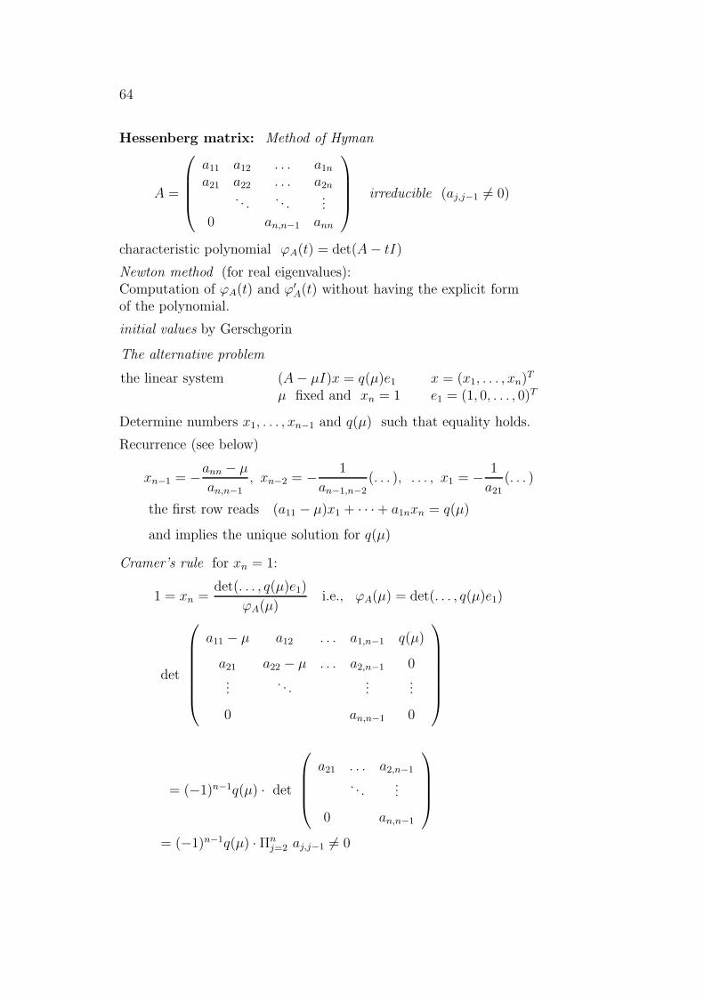
64
Hessenberg matrix: Method of Hyman
A =
a11 a12 . . . a1n
a21 a22 . . . a2n
. . .. . .
...0 an,n−1 ann
irreducible (aj,j−1 6= 0)
characteristic polynomial ϕA(t) = det(A− tI)
Newton method (for real eigenvalues):Computation of ϕA(t) and ϕ′A(t) without having the explicit formof the polynomial.
initial values by Gerschgorin
The alternative problem
the linear system (A− µI)x = q(µ)e1 x = (x1, . . . , xn)T
µ fixed and xn = 1 e1 = (1, 0, . . . , 0)T
Determine numbers x1, . . . , xn−1 and q(µ) such that equality holds.
Recurrence (see below)
xn−1 = −ann − µan,n−1
, xn−2 = − 1
an−1,n−2(. . . ), . . . , x1 = − 1
a21(. . . )
the first row reads (a11 − µ)x1 + · · ·+ a1nxn = q(µ)
and implies the unique solution for q(µ)
Cramer’s rule for xn = 1:
1 = xn =det(. . . , q(µ)e1)
ϕA(µ)i.e., ϕA(µ) = det(. . . , q(µ)e1)
det
a11 − µ a12 . . . a1,n−1 q(µ)
a21 a22 − µ . . . a2,n−1 0...
. . ....
...
0 an,n−1 0
= (−1)n−1q(µ) · det
a21 . . . a2,n−1
. . ....
0 an,n−1
= (−1)n−1q(µ) · Πnj=2 aj,j−1 6= 0

8. EIGENVALUES OF SYMMETRIC MATRICES 65
Result: ϕA(µ) = constant · q(µ)
i.e., λ zero of q(µ) if and only if λ eigenvalue of A.
q(µ) is implicitly defined by the linear system
−q(µ) + (a11 − µ)x1 + a12x2 + . . . +a1,n−1 xn−1 = −a1n
a21 x1 + (a22 − µ)x2 + . . . +a2,n−1 xn−1 = −a2n
. . ....
...an,n−1 xn−1 = −(ann − µ)
q(µ) will be computed by recurrence (from below)
Derivative: x′j = x′j(µ)
−q′(µ) + (a11 − µ)x′1 + a12x′2 + . . . +a1,n−1 x
′n−1 = x1
a21 x′1 + (a22 − µ)x′2 + . . . +a2,n−1 x
′n−1 = x2
. . ....
...an,n−1 x
′n−1 = xn = 1
q′(µ) will be computed by recurrence (from below)
Newton method µk+1 := µk − q(µk)q′(µk)
, k = 0, 1, . . .
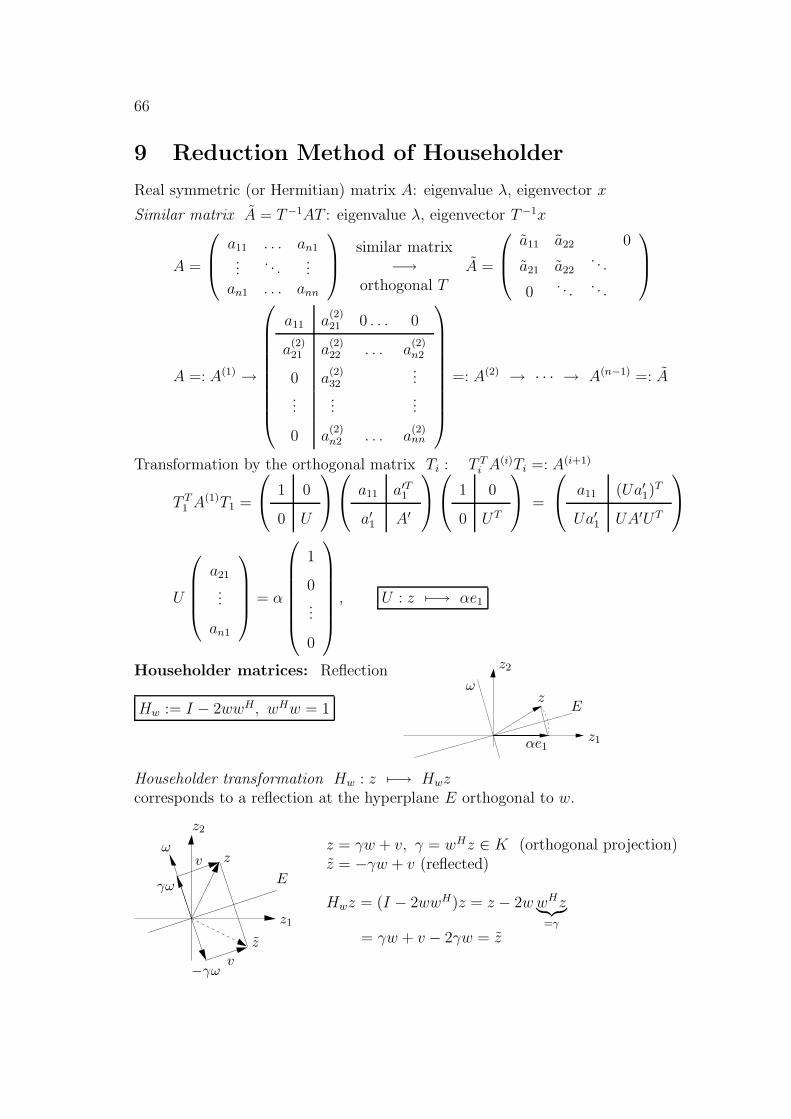
66
9 Reduction Method of Householder
Real symmetric (or Hermitian) matrix A: eigenvalue λ, eigenvector x
Similar matrix A = T−1AT : eigenvalue λ, eigenvector T−1x
A =
a11 . . . an1...
. . ....
an1 . . . ann
similar matrix−→
orthogonal TA =
a11 a22 0
a21 a22. . .
0. . .
. . .
A =: A(1) →
a11 a(2)21 0 . . . 0
a(2)21 a
(2)22 . . . a
(2)n2
0 a(2)32
......
......
0 a(2)n2 . . . a
(2)nn
=: A(2) → · · · → A(n−1) =: A
Transformation by the orthogonal matrix Ti : T Ti A(i)Ti =: A(i+1)
T T1 A(1)T1 =
1 0
0 U
a11 a′T1
a′1 A′
1 0
0 UT
=
a11 (Ua′1)T
Ua′1 UA′UT
U
a21
...
an1
= α
1
0...
0
, U : z 7−→ αe1
Householder matrices: Reflection
Hw := I − 2wwH, wHw = 1
PSfrag replacements
ω
z2
zE
z1αe1
Householder transformation Hw : z 7−→ Hwzcorresponds to a reflection at the hyperplane E orthogonal to w.
PSfrag replacements
−γω v
z
z1
E
zvω
γω
z2
z = γw + v, γ = wHz ∈ K (orthogonal projection)z = −γw + v (reflected)
Hwz = (I − 2wwH)z = z − 2wwHz︸︷︷︸=γ
= γw + v − 2γw = z
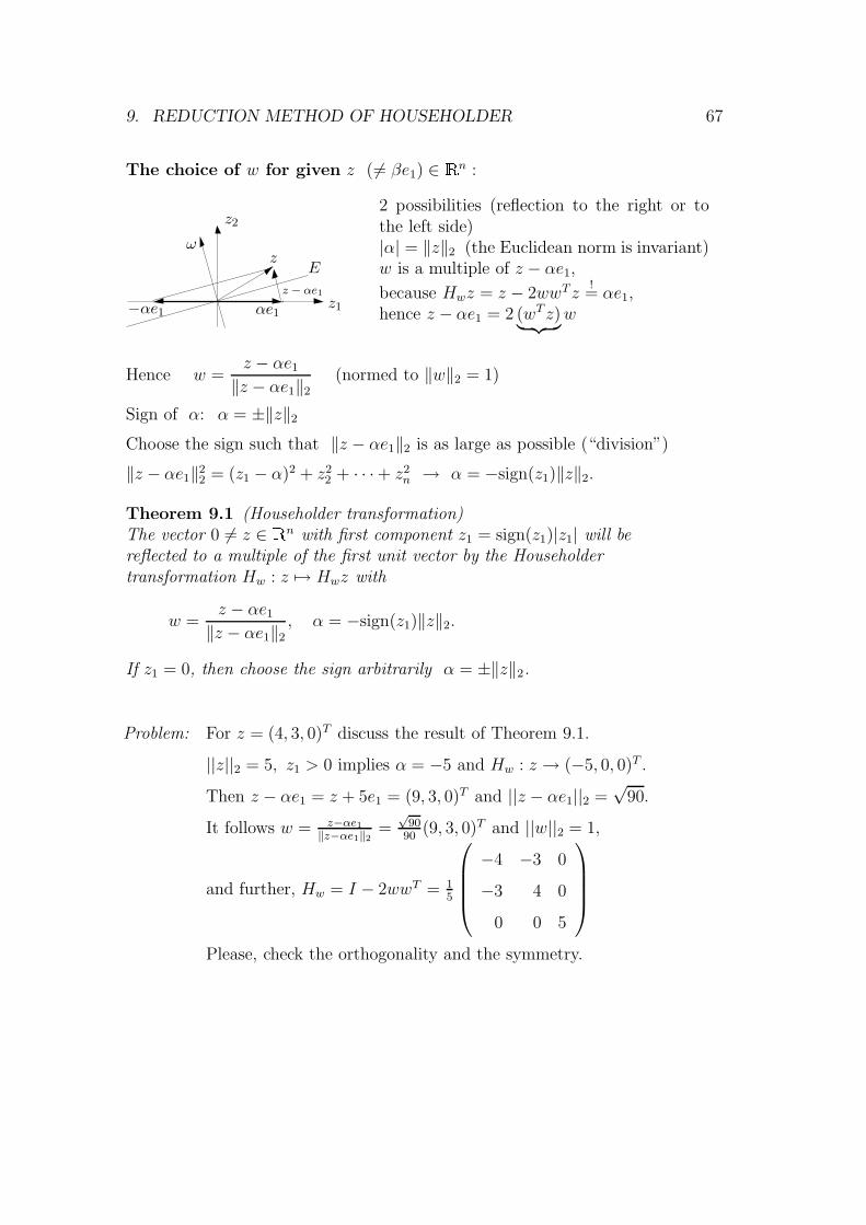
9. REDUCTION METHOD OF HOUSEHOLDER 67
The choice of w for given z (6= βe1) ∈ � n :
PSfrag replacements
ω
z2
zE
z1αe1
z − αe1−αe1
2 possibilities (reflection to the right or tothe left side)|α| = ‖z‖2 (the Euclidean norm is invariant)w is a multiple of z − αe1,
because Hwz = z − 2wwTz!
= αe1,hence z − αe1 = 2 (wTz)︸ ︷︷ ︸w
Hence w =z − αe1
‖z − αe1‖2(normed to ‖w‖2 = 1)
Sign of α: α = ±‖z‖2
Choose the sign such that ‖z − αe1‖2 is as large as possible (“division”)
‖z − αe1‖22 = (z1 − α)2 + z2
2 + · · ·+ z2n → α = −sign(z1)‖z‖2.
Theorem 9.1 (Householder transformation)The vector 0 6= z ∈ � n with first component z1 = sign(z1)|z1| will bereflected to a multiple of the first unit vector by the Householdertransformation Hw : z 7→ Hwz with
w =z − αe1
‖z − αe1‖2
, α = −sign(z1)‖z‖2.
If z1 = 0, then choose the sign arbitrarily α = ±‖z‖2.
Problem: For z = (4, 3, 0)T discuss the result of Theorem 9.1.
||z||2 = 5, z1 > 0 implies α = −5 and Hw : z → (−5, 0, 0)T .
Then z − αe1 = z + 5e1 = (9, 3, 0)T and ||z − αe1||2 =√
90.
It follows w = z−αe1‖z−αe1‖2 =
√90
90(9, 3, 0)T and ||w||2 = 1,
and further, Hw = I − 2wwT = 15
−4 −3 0
−3 4 0
0 0 5
Please, check the orthogonality and the symmetry.
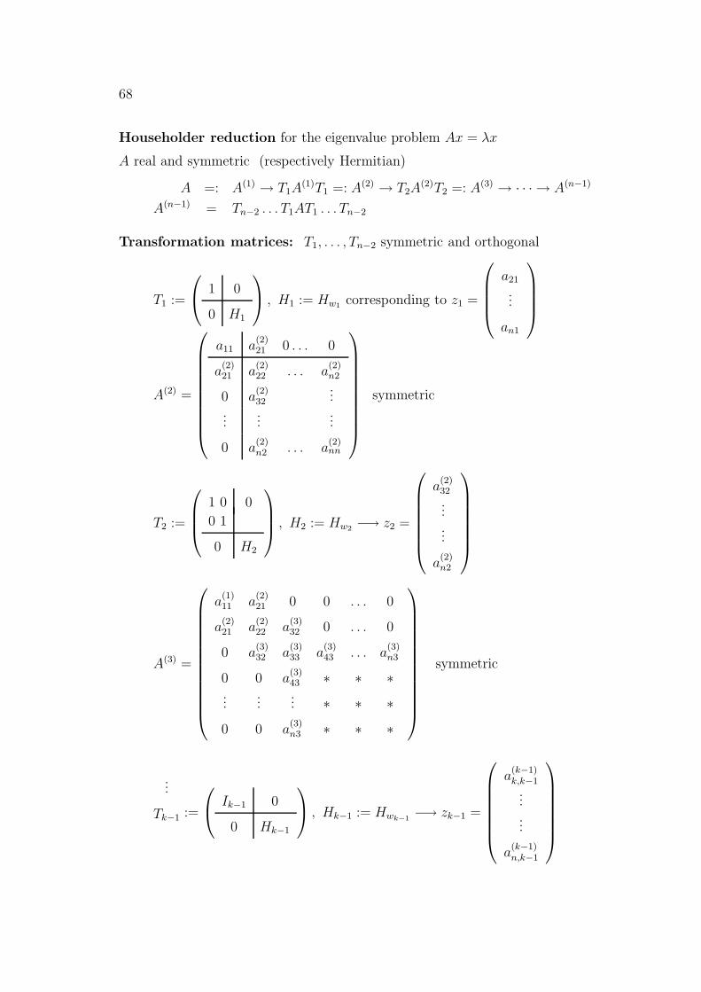
68
Householder reduction for the eigenvalue problem Ax = λx
A real and symmetric (respectively Hermitian)
A =: A(1) → T1A(1)T1 =: A(2) → T2A
(2)T2 =: A(3) → · · · → A(n−1)
A(n−1) = Tn−2 . . . T1AT1 . . . Tn−2
Transformation matrices: T1, . . . , Tn−2 symmetric and orthogonal
T1 :=
1 0
0 H1
, H1 := Hw1 corresponding to z1 =
a21
...
an1
A(2) =
a11 a(2)21 0 . . . 0
a(2)21 a
(2)22 . . . a
(2)n2
0 a(2)32
......
......
0 a(2)n2 . . . a
(2)nn
symmetric
T2 :=
1 0 0
0 1
0 H2
, H2 := Hw2 −→ z2 =
a(2)32
...
...
a(2)n2
A(3) =
a(1)11 a
(2)21 0 0 . . . 0
a(2)21 a
(2)22 a
(3)32 0 . . . 0
0 a(3)32 a
(3)33 a
(3)43 . . . a
(3)n3
0 0 a(3)43 ∗ ∗ ∗
......
... ∗ ∗ ∗0 0 a
(3)n3 ∗ ∗ ∗
symmetric
...
Tk−1 :=
Ik−1 0
0 Hk−1
, Hk−1 := Hwk−1
−→ zk−1 =
a(k−1)k,k−1
...
...
a(k−1)n,k−1
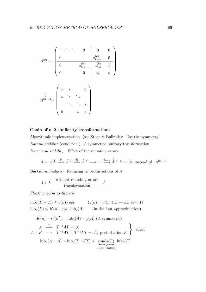
9. REDUCTION METHOD OF HOUSEHOLDER 69
A(k) :=
. . .. . .
. . . 0 0 0
0 a(k)k,k−1 0
0 a(k])k,k−1 a
(k)k,k zTk
0 0 zk ∗
...A(n−1)=
∗ ∗ 0
∗ . . .. . .
. . .. . . ∗
0 ∗ ∗
Chain of n–2 similarity transformations
Algorithmic implementation (see Stoer & Bulirsch): Use the symmetry!
Natural stability (condition:) A symmetric, unitary transformation
Numerical stability: Effect of the rounding errors
A =: A(1) T1−→ A(2) T2−→ ˜A(3) −→ · · · Tn−2−→ ˜A(n−1) =: A instead of A(n−1)
Backward analysis: Reducing to perturbations of A
A+ Fwithout rounding errors−−−−−−−−−−→transformation
A
Floating–point arithmetic
lub2(Ti − Ti) ≤ g(n) · eps (g(n) = O(nα), n→∞, α ≈ 1)
lub2(F )·≤ K(n) · eps · lub2(A) (in the first approximation)
K(n) = O(n2), lub2(A) = ρ(A) (A symmetric)
AT−→ T−1AT =: A
A+ F −→ T−1AT + T−1FT =: A, perturbation F
}effect
lub2(A− A) = lub2(T−1FT ) ≤ cond2(T )︸ ︷︷ ︸=1 (T unitary)
lub2(F )
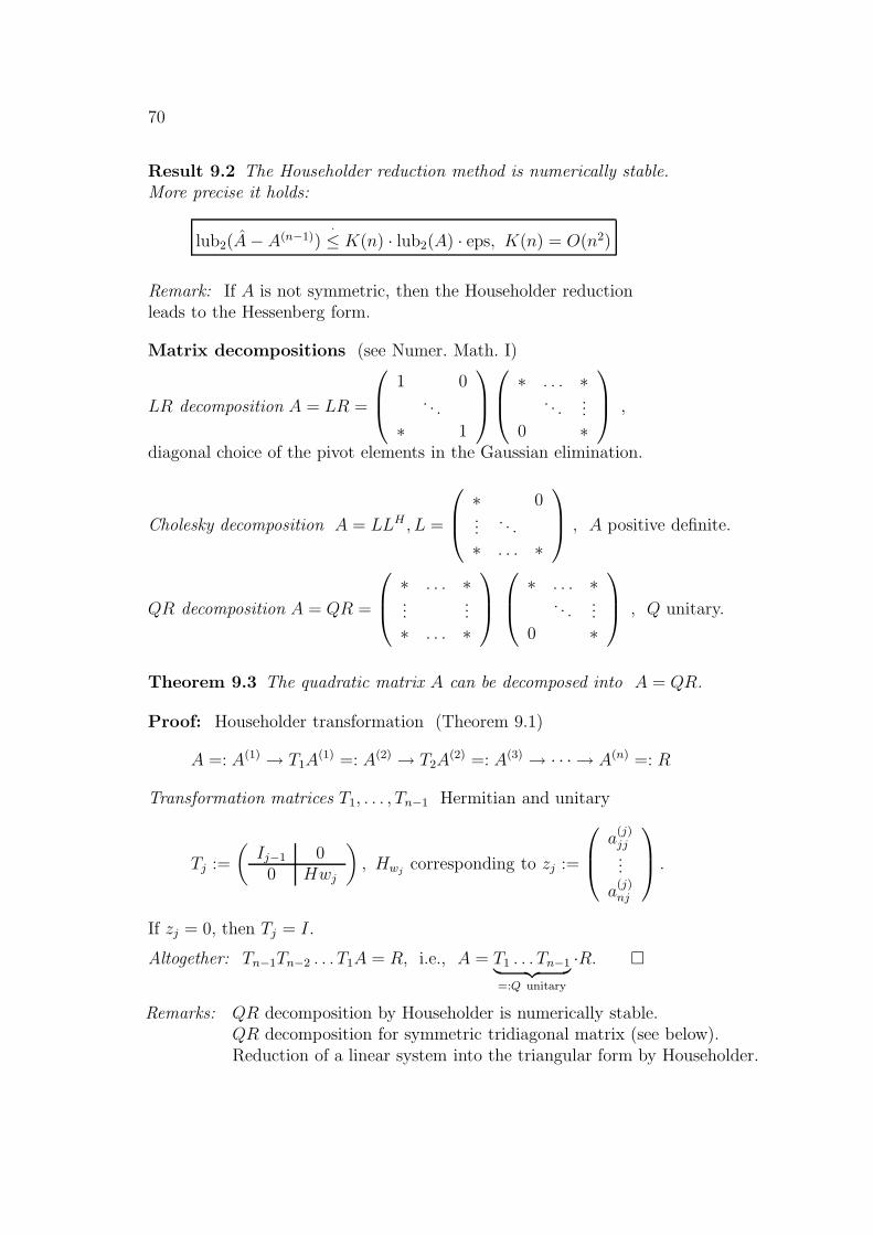
70
Result 9.2 The Householder reduction method is numerically stable.More precise it holds:
lub2(A− A(n−1))·≤ K(n) · lub2(A) · eps, K(n) = O(n2)
Remark: If A is not symmetric, then the Householder reductionleads to the Hessenberg form.
Matrix decompositions (see Numer. Math. I)
LR decomposition A = LR =
1 0. . .
∗ 1
∗ . . . ∗
. . ....
0 ∗
,
diagonal choice of the pivot elements in the Gaussian elimination.
Cholesky decomposition A = LLH , L =
∗ 0...
. . .
∗ . . . ∗
, A positive definite.
QR decomposition A = QR =
∗ . . . ∗...
...∗ . . . ∗
∗ . . . ∗
. . ....
0 ∗
, Q unitary.
Theorem 9.3 The quadratic matrix A can be decomposed into A = QR.
Proof: Householder transformation (Theorem 9.1)
A =: A(1) → T1A(1) =: A(2) → T2A
(2) =: A(3) → · · · → A(n) =: R
Transformation matrices T1, . . . , Tn−1 Hermitian and unitary
Tj :=
(Ij−1 0
0 Hwj
), Hwj corresponding to zj :=
a(j)jj...
a(j)nj
.
If zj = 0, then Tj = I.
Altogether: Tn−1Tn−2 . . . T1A = R, i.e., A = T1 . . . Tn−1︸ ︷︷ ︸=:Q unitary
·R. �
Remarks: QR decomposition by Householder is numerically stable.QR decomposition for symmetric tridiagonal matrix (see below).Reduction of a linear system into the triangular form by Householder.
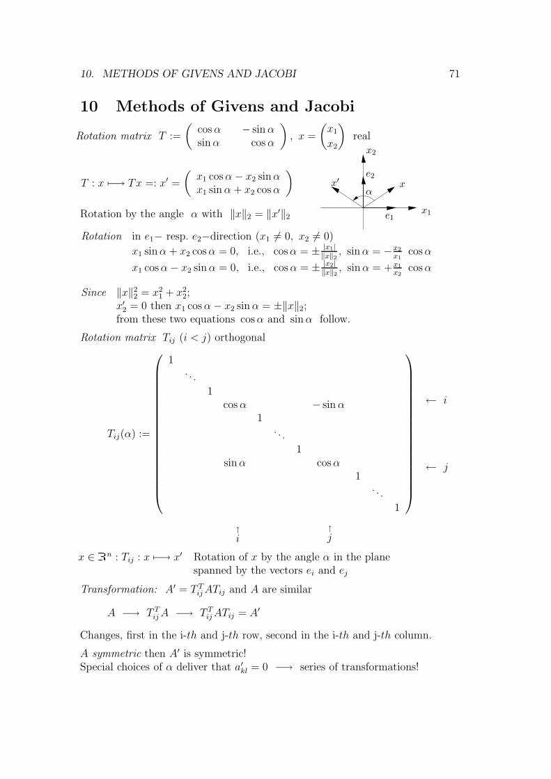
10. METHODS OF GIVENS AND JACOBI 71
10 Methods of Givens and Jacobi
Rotation matrix T :=
(cosα − sinαsinα cosα
), x =
(x1
x2
)real
T : x 7−→ Tx =: x′ =
(x1 cosα− x2 sinαx1 sinα + x2 cosα
)
Rotation by the angle α with ‖x‖2 = ‖x′‖2
PSfrag replacements
e1x1
xα
e2
x2
x′
Rotation in e1− resp. e2−direction (x1 6= 0, x2 6= 0)
x1 sinα + x2 cosα = 0, i.e., cosα = ± |x1|‖x‖2 , sinα = −x2
x1cosα
x1 cosα− x2 sinα = 0, i.e., cosα = ± |x2|‖x‖2 , sinα = +x1
x2cosα
Since ‖x‖22 = x2
1 + x22;
x′2 = 0 then x1 cosα− x2 sinα = ±‖x‖2;from these two equations cosα and sinα follow.
Rotation matrix Tij (i < j) orthogonal
Tij(α) :=
1. . .
1cosα − sinα
1. . .
1sinα cosα
1. . .
1
← i
← j
↑i
↑j
x ∈ � n : Tij : x 7−→ x′ Rotation of x by the angle α in the planespanned by the vectors ei and ej
Transformation: A′ = T TijATij and A are similar
A −→ T TijA −→ T TijATij = A′
Changes, first in the i-th and j-th row, second in the i-th and j-th column.
A symmetric then A′ is symmetric!Special choices of α deliver that a′kl = 0 −→ series of transformations!
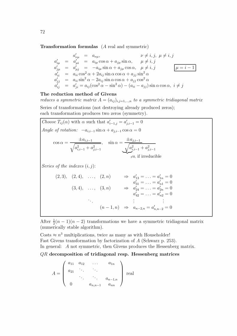
72
Transformation formulas (A real and symmetric)
a′νµ = aνµ, ν 6= i, j, µ 6= i, ja′iµ = a′µi = aiµ cosα + ajµ sinα, µ 6= i, j
a′jµ = a′µj = −aiµ sinα + ajµ cosα, µ 6= i, j µ = i− 1
a′ii = aii cos2 α + 2aij sinα cosα+ ajj sin2 αa′jj = aii sin
2 α− 2aij sinα cosα + ajj cos2 αa′ij = a′ji = aij(cos2 α− sin2 α)− (aii − ajj) sinα cosα, i 6= j
The reduction method of Givensreduces a symmetric matrix A = (aij)i,j=1,...,n to a symmetric tridiagonal matrix
Series of transformations (not destroying already produced zeros);each transformation produces two zeros (symmetry).
Choose Tij(α) with α such that a′i−1,j = a′j,i−1 = 0
Angle of rotation: −ai,i−1 sinα + aj,i−1 cosα = 0
cosα =±ai,i−1√
a2i,i−1 + a2
j,i−1
, sinα =±aj,i−1√a2i,i−1 + a2
j,i−1︸ ︷︷ ︸6=0, if irreducible
Series of the indexes (i, j):
(2, 3), (2, 4), . . . , (2, n) ⇒ a′13 = . . . = a′1n = 0a′31 = . . . = a′n1 = 0
(3, 4), . . . , (3, n) ⇒ a′24 = . . . = a′2n = 0a′42 = . . . = a′n2 = 0
. . ....
...(n− 1, n) ⇒ an−2,n = a′n,n−2 = 0
After 12(n − 1)(n − 2) transformations we have a symmetric tridiagonal matrix
(numerically stable algorithm).
Costs ≈ n3 multiplications, twice as many as with Householder!Fast Givens transformation by factorization of A (Schwarz p. 253).In general: A not symmetric, then Givens produces the Hessenberg matrix.
QR decomposition of tridiagonal resp. Hessenberg matrices
A =
a11 a12 . . . a1n
a21. . .
. . .. . .
. . . an−1,n
0 an,n−1 ann
real
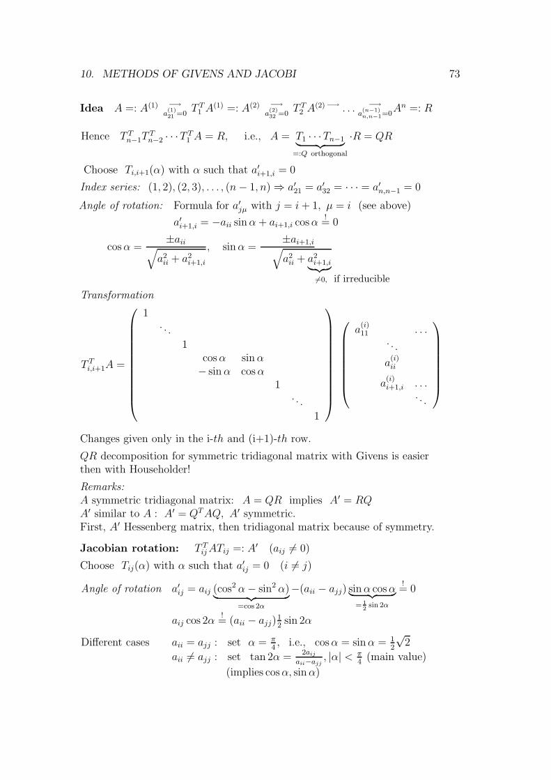
10. METHODS OF GIVENS AND JACOBI 73
Idea A =: A(1) −→a
(1)21 =0
T T1 A(1) =: A(2) −→
a(2)32 =0
T T2 A(2)−→ . . . −→
a(n−1)n,n−1=0
An =: R
Hence T Tn−1TTn−2 · · ·T T1 A = R, i.e., A = T1 · · ·Tn−1︸ ︷︷ ︸
=:Q orthogonal
·R = QR
Choose Ti,i+1(α) with α such that a′i+1,i = 0
Index series: (1, 2), (2, 3), . . . , (n− 1, n)⇒ a′21 = a′32 = · · · = a′n,n−1 = 0
Angle of rotation: Formula for a′jµ with j = i + 1, µ = i (see above)
a′i+1,i = −aii sinα + ai+1,i cosα!
= 0
cosα =±aii√
a2ii + a2
i+1,i
, sinα =±ai+1,i√a2ii + a2
i+1,i︸ ︷︷ ︸6=0, if irreducible
Transformation
T Ti,i+1A =
1. . .
1cosα sinα− sinα cosα
1. . .
1
a(i)11 . . .
. . .
a(i)ii
a(i)i+1,i . . .
. . .
Changes given only in the i-th and (i+1)-th row.
QR decomposition for symmetric tridiagonal matrix with Givens is easierthen with Householder!
Remarks:A symmetric tridiagonal matrix: A = QR implies A′ = RQA′ similar to A : A′ = QTAQ, A′ symmetric.First, A′ Hessenberg matrix, then tridiagonal matrix because of symmetry.
Jacobian rotation: T TijATij =: A′ (aij 6= 0)
Choose Tij(α) with α such that a′ij = 0 (i 6= j)
Angle of rotation a′ij = aij (cos2 α− sin2 α)︸ ︷︷ ︸=cos 2α
−(aii − ajj) sinα cosα︸ ︷︷ ︸= 1
2sin 2α
!= 0
aij cos 2α!
= (aii − ajj)12
sin 2α
Different cases aii = ajj : set α = π4, i.e., cosα = sinα = 1
2
√2
aii 6= ajj : set tan 2α =2aij
aii−ajj , |α| <π4
(main value)
(implies cosα, sinα)
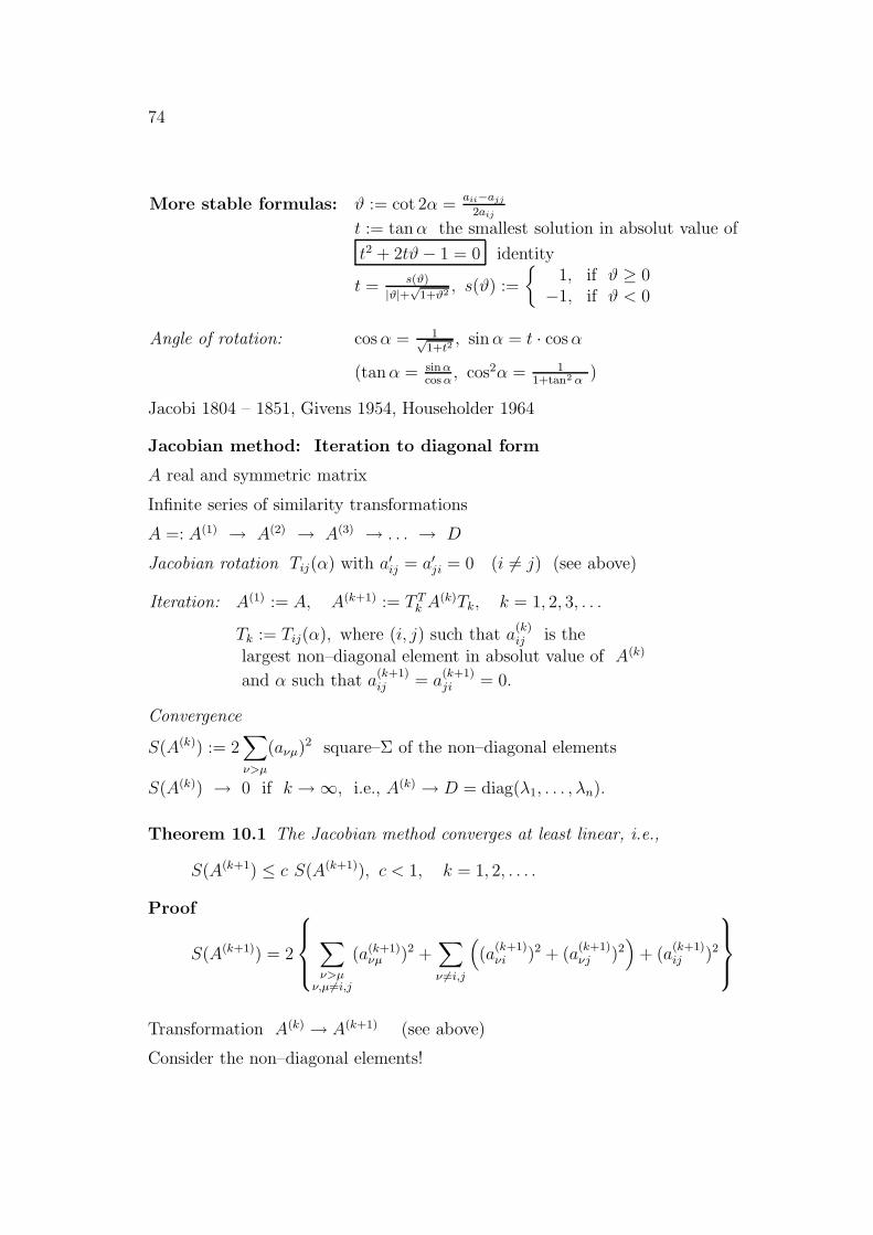
74
More stable formulas: ϑ := cot 2α =aii−ajj
2aij
t := tanα the smallest solution in absolut value of
t2 + 2tϑ− 1 = 0 identity
t = s(ϑ)
|ϑ|+√
1+ϑ2 , s(ϑ) :=
{1, if ϑ ≥ 0−1, if ϑ < 0
Angle of rotation: cosα = 1√1+t2
, sinα = t · cosα
(tanα = sinαcosα
, cos2α = 11+tan2 α
)
Jacobi 1804 – 1851, Givens 1954, Householder 1964
Jacobian method: Iteration to diagonal form
A real and symmetric matrix
Infinite series of similarity transformations
A =: A(1) → A(2) → A(3) → . . . → D
Jacobian rotation Tij(α) with a′ij = a′ji = 0 (i 6= j) (see above)
Iteration: A(1) := A, A(k+1) := T Tk A(k)Tk, k = 1, 2, 3, . . .
Tk := Tij(α), where (i, j) such that a(k)ij is the
largest non–diagonal element in absolut value of A(k)
and α such that a(k+1)ij = a
(k+1)ji = 0.
Convergence
S(A(k)) := 2∑
ν>µ
(aνµ)2 square–Σ of the non–diagonal elements
S(A(k)) → 0 if k →∞, i.e., A(k) → D = diag(λ1, . . . , λn).
Theorem 10.1 The Jacobian method converges at least linear, i.e.,
S(A(k+1) ≤ c S(A(k+1)), c < 1, k = 1, 2, . . . .
Proof
S(A(k+1)) = 2
∑
ν>µν,µ 6=i,j
(a(k+1)νµ )2 +
∑
ν 6=i,j
((a
(k+1)νi )2 + (a
(k+1)νj )2
)+ (a
(k+1)ij )2
Transformation A(k) → A(k+1) (see above)
Consider the non–diagonal elements!

10. METHODS OF GIVENS AND JACOBI 75
The first sum: There are no changes in the coefficients!
The second sum: a(k+1)νij
= a(k)νijcosα± a(k)
νji
sinα (symmetry a(k)νii
= a(k)iνj
)
(a(k+1)νij
)2 = (a(k)νij)2 cos2 α + (aνj
i)2 sin2 α± 2a
(k)νi a
(k)νj sinα cosα
Addition of the two equations yields
(a(k+1)νi )2 + (a
(k+1)νj )2 = (a
(k)νi )2 + (a
(k)νj )2
i.e., there are no changes in the sums.
The third sum: a(k)ij the largest non–diagonal element in absolut value,
i.e., a(k+1)ij = 0
Hence, it follows S(A(k+1)) < S(A(k)).
Consider a rough estimation for the constant c
S(A(k)) ≤ n(n− 1)(a(k)ij )2
(number of the non–diagonal elements × largest element in absolut valueto the square) or
(a(k)ij )2 ≥ 1
n(n− 1)S(A(k)).
Hence, it follows
S(A(k+1)) ≤ S(A(k))− 2(a(k)ij )2
≤ S(A(k))− 2
n(n− 1)S(A(k)) = (1− 2
n(n− 1))
︸ ︷︷ ︸=:c
S(A(k))
with 0 ≤ c < 1. �
Theorem 10.2 (Error bound)Let λ1 ≤ · · · ≤ λn be the eigenvalues of the symmetric matrix A and
d(k)1 ≤ d
(k)2 ≤ · · · ≤ d(k)
n
the diagonal elements a(k)jj of A(k). Then it follows
maxj|d(k)j − λj| ≤
√S(A(k)), k = 1, 2, . . . .
Remarks
i) Stopping criterion with a given accuracy ε:
S(A(k)) ≤ ε2 or simple n(n− 1)|a(k)ij |2 ≤ ε2
76
ii) The Jacobian method converges quadratically: S(A(k+1)) ≤ c(S(A(k))
)2,
as soon as the non–diagonal elements are sufficiently small in absolut value(→ local convergency, c.f. Newton’s method)!
iii) The structure of a sparse matrix will be destroyedby the Jacobian method!
The cyclic Jacobian methodInstead of determining the largest non–diagonal element in absolut value, choosea fixed index series, which will be repeated several times:
(1, 2) (1, 3) . . . (1, n)
(2, 3) . . . (2, n). . .
...
(n− 1, n)
1 cycle
Convergence behaviour as in the classical case, but more costs(a difficult proof)!
Computation of the eigenvectors by the Jacobian method
A(k+1) = T Tk A(k)Tk = T Tk . . . T
T1 AT1 . . . Tk =: V T
k AVk
Vk := T1 . . . Tk orthogonal
Theorem 7.1 implies that the symmetric matrix A is orthogonallydiagonalizable, i.e., UTAU = diag(λ1, . . . , λn), U = (x1, . . . , xn),xj orthogonal eigenvector of the eigenvalue λj (j = 1, . . . , n).Hence A(k+1) = V T
k AVk approximates diag(λ1, . . . , λn), and the columnvectors of Vk approximates the eigenvectors of the eigenvalues λk.
Summary
The Jacobian method for real and symmetric matrices:Iterative computation of all eigenvalues and the corresponding eigenvectorsThe matrix Tk will be chosen classically or the cyclic version is usedStopping criterion is used or a given number of cycles is chosenApproximation for the eigenvalues λj: diagonal elements a
(k+1)jj
Approximation for the eigenvectors xj: column vectors v(k)j of Vk
Local quadratic convergence for k ≥ m0
The structure of a sparse matrix (tridiagonal matrix) will be destroyed
11. VECTOR ITERATION OF MISES AND WIELANDT 77
11 Vector Iteration of Mises and Wielandt
Raising the dominant eigenvalue to a high power: Akx = λkx
Assumption: A a real matrix with dominant eigenvalue λ1 and eigenvector x1,
A diagonalizable (n linearily independent eigenvectors)
(the assumptions can be essentially weaker)
Vector iteration z(k+1) := Az(k) = Ak+1z(0), k = 0, 1, 2, . . .
Theorem 11.1 The vector iteration converges linearily with a suitable initialvector z(0), i.e., if k → ∞ the vectors z(k) become parallel to the eigenvectorx1 and the quotients z
(k+1)j /z
(k)j converge to λ1 (for suitable components z
(k)j 6=
0, x1j 6= 0).
ProofEigenvalues |λ1| > |λ2| ≥ · · · ≥ |λn|Eigenvectors x1, . . . , xn linearily independent (a simplification)
Initial vector z(0) = α1x1 + · · ·+ αnxn (z(0) suitable, i.e., α1 6= 0)
Iteration z(k+1) = Ak+1z(0) = α1λk+11 x1 + · · ·+ αnλ
k+1n xn
= α1λk+11 xk+1
1 {x1 +α2
α1
(λ2
λ1
)k+1
︸ ︷︷ ︸→0
x2 + · · ·+ αnα1
(λnλ1
)k+1
︸ ︷︷ ︸→0
xn}
z(k+1)j /z
(k)j → λ1 (z
(k)j 6= 0, x1j 6= 0) if k →∞ �
Example
A =
1 4
2 3
, z(0) =
1
0
, z(1) =
1
2
, z(2) =
9
8
, z(3) =
41
42
,
z(4) =
209
208
, z5 =
1041
1042
, . . .
quotients (j = 1): 9, 4.55 . . . , 5.097 . . . , 4.9808 . . . , . . .quotients (j = 2): 4, 5.25 . . . , 4.952 . . . , 5.0096, . . . , . . .
The eigenvalues are λ1 = 5 λ2 = 1;
the eigenvectors are x1 =
1
1
, x2 =
2
−1
.
78
Remarks The speed of convergence depends on the factor∣∣∣λ2
λ1
∣∣∣.The initial vector can easily be found (because
of rounding errors we usually have α1 6= 0).
The normalization of the vectors z(k) is convenient.
The method of Mises
Initial vector y(0) with ‖y(0)‖ = 1 (α1 6= 0, z.B. ‖ · ‖∞)
y(k+1) := Ay(k), y(k+1) := y(k+1)
‖y(k+1)‖ , k = 0, 1, 2, . . .
y(k+1)j /y
(k+1)j → λ1 if k →∞
(signλ1)ky(k) → α1x1
‖α1x1‖ if k →∞Linear convergence with the factor q :=
∣∣∣λ2
λ1
∣∣∣ < 1 :
y(k+1)j /y
(k)j = λ1 +O(qk) (k →∞).
Modifications1. A not diagonalizable2. complex eigenvalue λ1 = |λ1|eiϕ1
3. dominant eigenvalue of multiplicity p4. distinct dominant eigenvalues5. raising the zeros of a polynomial to high power
Acceleration of convergence
Rayleigh quotient rA(z) = zHAzzHz
Series {z(k)}k≥0 resp. {y(k)}k≥0
New series
{rA(z(k))}k≥0 with rA(z(k)) =(z(k))Hz(k+1)
(z(k))Hz(k)=
(y(k))H y(k+1)
(y(k))Hy(k)
Theorem 11.2 Let A be Hermitian with eigenvalues |λ1| > |λ2| ≥ · · · ≥ |λn|,then
rA(z(k)) = λ1 +O(q2k) (k →∞).
ProofReal eigenvalues, linearily independent orthogonal eigenvectors (Th. 7.1)
z(0) = α1x1 + · · ·+ αnxn (α1 6= 0), {x1, . . . , xn} orthogonal normalized system
z(k) = α1λk1x1 + · · ·+ αnλ
knxn
11. VECTOR ITERATION OF MISES AND WIELANDT 79
(z(k))Hz(k) =
(∑
ν
ανλkνx
Hν
)(∑
µ
αµλkµxµ
)=∑
ν
|αν|2λ2kν
= |α1|2λ2k1
1 +
∑
ν
|ανα1|2(λνλ1
)2k
︸ ︷︷ ︸→0
(z(k))Hz(k+1) = · · · = |α1|2λ2k+11
1 +
∑ |ανα1|2(λνλ1
)2k+1
︸ ︷︷ ︸→0
rA(z(k)) = λ1
1 +∑n
ν=2 |ανα1|2(λν
λ1)2k+1
1 +∑n
ν=2 |ανα1|2(λν
λ1)2k
= λ1(1 +O(q2k)) = λ1 +O(q2k) (k →∞) �
The inverse iteration of Wielandt
Application of the vector iteration to A−1 (A nonsingular)
z(k+1) := A−1z(k), k = 0, 1, 2, . . . (z(0) suitable)
yields the inverse of the largest eigenvalue of A in absolut value.
Instead of computing A−1, the linear system Az(k+1) = z(k) will be solved:
A = LR, Lv(k) = z(k), Rz(k+1) = v(k) (with normalization).
Eigenvalues |λ1| > |λ2| > · · · > |λn−1| > |λn|
Factor of convergence
∣∣∣∣λ2
λ1
∣∣∣∣ respectively
∣∣∣∣λnλn−1
∣∣∣∣Shift: shift of the eigenvalues
Matrix As := A− sI with shift parameter s
λ eigenvalue of A if and only if λ− s eigenvalue of As
i) Acceleration of convergence:
s such that
∣∣∣∣λn − sλn−1 − s
∣∣∣∣ <∣∣∣∣λnλn−1
∣∣∣∣
ii) Computation of the eigenvalues λj (j ∈ {1, 2, . . . , n}) :s such that |λj − s| < |λk − s| for all k 6= j
Then the inverse iteration is applied to As
Choice of the shift parameter:An approximation tj of λj is known, then choose s = tj;fitting of the parameter s after some steps!
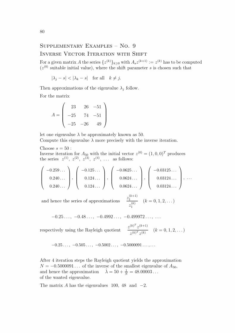
80
Supplementary Examples – No. 9
Inverse Vector Iteration with Shift
For a given matrix A the series {z(k)}k≥0 with Asz(k+1) := z(k) has to be computed
(z(0) suitable initial value), where the shift parameter s is chosen such that
|λj − s| < |λk − s| for all k 6= j.
Then approximations of the eigenvalue λj follow.
For the matrix
A =
23 26 −51
−25 74 −51
−25 −26 49
let one eigenvalue λ be approximately known as 50.Compute this eigenvalue λ more precisely with the inverse iteration.
Choose s = 50 :Inverse iteration for A50 with the initial vector z(0) = (1, 0, 0)T producesthe series z(1), z(2), z(3), z(4), . . . as follows:
−0.259 . . .
0.240 . . .
0.240 . . .
,
−0.125 . . .
0.124 . . .
0.124 . . .
,
−0.0625 . . .
0.0624 . . .
0.0624 . . .
,
−0.03125 . . .
0.03124 . . .
0.03124 . . .
, . . .
and hence the series of approximationsz
(k+1)1
z(k)1
(k = 0, 1, 2, . . . )
−0.25 . . . , −0.48 . . . , −0.4992 . . . , −0.499972 . . . , . . .
respectively using the Rayleigh quotientz(k)T z(k+1)
z(k)T z(k)(k = 0, 1, 2, . . . )
−0.25 . . . , −0.505 . . . , −0.5002 . . . , −0.5000091 . . . , . . .
After 4 iteration steps the Rayleigh quotient yields the approximationN = −0.5000091 . . . of the inverse of the smallest eigenvalue of A50,and hence the approximation λ = 50 + 1
N= 48.00003 . . .
of the wanted eigenvalue.
The matrix A has the eigenvalues 100, 48 and −2.
12. LR AND QR METHOD 81
12 LR and QR method
Iteration method with the series {Ak}k≥1 and Ak →
λ1 ∗. . .
0 λn
Similarity transformations using LR and QR decompositions!Compute simultaneously the eigenvalues and the eigenvectors!
Idea: Raising A to a high power Ak similar to the vector iteration
Factorization Ak = LkRk (LR decomposition)
Refinement: compute all eigenvalues λ1, . . . , λn
Application: Symmetric and non–symmetric matricesFirst, reduction to symmetric tridiagonal respectively Hessenberg matrix,LR resp. QR decomposition is simpler and the structure is preserved.
LR method
Assumption: Real nonsingular matrix A with |λ1| > · · · > |λn| > 0
Existence of the necessary LR decompositions
Algorithm: A1 := A
Ak =: LkRk, Ak+1 := RkLk, k = 1, 2, . . .
i) Similarity transformation
Ak+1 = L−1k AkLk = (L1 . . . Lk)
−1A(L1 . . . Lk) (cond (Lk) =?)
ii) Factorization of Ak:
Ak = L1 . . . Lk︸ ︷︷ ︸ Rk . . . R1︸ ︷︷ ︸ =: LkRk
Since A = A1 = L1R1, A2 = L2R2, . . .
Ak = L1(R1L1︸ ︷︷ ︸A2
)(R1 . . . L1)R1 = L1Ak−12 R1
= L1(L2(R2L2︸ ︷︷ ︸A3
)(R2 . . . L2)R2)R1 = L1L2Ak−23 R2R1
= L1 . . . Lk−1AkRk−1 . . . R1
= (L1 . . . Lk−1Lk)(RkRk−1 . . . R1) = LkRk
82
Hence Ak = LkRk , where
Lk = Lk−1Lk =
1 0. . .
∗ 1
, Rk = RkRk−1 =
r(k)11 ∗
. . .
0 r(k)nn
,
Rk =
r(k)11 ∗
. . .
0 r(k)nn
, r
(k)11 = r
(k)11 r
k−111 ,
vector iteration z(k) = Ake1 =
r
(k)11
...
, z
(k)1 /z
(k−1)1 = r
(k)11 ,
r(k)11 → λ1 if k →∞.
Under additional assumptions of A it follows
Rk →
λ1 ∗. . .
λn
, Ak →
λ1 ∗. . .
0 λn
, Lk → I if k →∞.
Theorem 12.1 (LR method) Let A = T diag (λ1, . . . , λn) T−1 withLR decomposable matrices T and T−1 and with
|λ1| > · · · > |λn| > 0.
Let the LR method be feasible for A, then
limk→∞
Ak = limk→∞
Rk =
λ1 ∗. . .
0 λn
, lim
k→∞Lk = I.
Proof: Investigation of the factorization of Ak
Ak = LkRk, Lk = Lk−1Lk, Rk = RkRk−1
Assumption on A: A = TDT−1, D := diag (λ1, . . . , λn), D−1 exists
T = LTRT , T−1 = LT−1RT−1
i > j : ( λiλj
)k → 0, k →∞.
12. LR AND QR METHOD 83
Lemmas
(1) Ak = TDkT−1 (= (TDT−1)k = TD T−1T︸ ︷︷ ︸DT−1 . . . T︸ ︷︷ ︸DT−1)
(2) DkLT−1D−k = I + Fk with Fk → 0 if k →∞(coefficients in the diagonal are one, below `ij(
λiλj
)k → 0 (i > j))
(3) RTFkR−1T → 0 if k →∞
(R−1T exists, because of RT = L−1
T T ; Fk → 0 if k →∞)
(4) Decomposition I +RTFkR−1T︸ ︷︷ ︸
→0
=: LkRk︸ ︷︷ ︸→I
exists for sufficiently large k
(5) Lk → I and Rk → I if k →∞.
Corollaries
a) Ak =(1)
TDkT−1 =assumption
LTRTDkLT−1RT−1 = LTRT (DkLT−1D−k︸ ︷︷ ︸)D
kRT−1
=(2)
LT (RT (I + Fk)R−1T )RTD
kRT−1 = LT (I +RTFkR−1T︸ ︷︷ ︸)RTD
kRT−1
=(4)
(LT Lk)(RkRTDkRT−1) =
↑uniqueness
1 0. . .
∗ 1
∗ . . . ∗
. . ....
0 ∗
= LkRk
b) Ak = LkRk (LR decomposition)
Lk = L−1k−1Lk =
(a)(LT Lk−1)−1(LT Lk) = L−1
k−1Lk →(5)
I if k →∞
Rk = RkR−1k−1 =
(a)(RkRTD
kRT−1)(Rk−1RTDk−1RT−1)−1
= Rk︸︷︷︸→I
RTDR−1T R−1
k−1︸ ︷︷ ︸→I
−→(5)
RTDR−1T =
λ1 . . . ∗
. . ....
0 λn
=: Rλ
c) Altogether
limk→∞
Ak = limk→∞
LkRk = Rλ. �
84
Remarks
1. The method breaks down, if Ak is not LR decomposable, and in generalit does not converge, if T or T−1 is not LR decomposable.
2. The computation of the LR decomposition can be ill–conditioned.
3. If the quotients |λi+1
λi| are close to 1, then the convergence is slow.
Shift techniques can accelerate the convergence.
4. Stopping criterion: maxν>µ|a(k)νµ | ≤ δ (δ given)
5. Numerical stability of the method (compare with cond(Lk)): Gaussianelimination method without pivot searching is not always stable!
6. If A symmetric, then Ak → diag(λ1, . . . , λn) if k →∞.
7. Expensive: one step Ak → Ak+1 needs 23n3 multiplications;
therefore application mostly on reduced matrices: Tridiagonalor Hessenberg form (this structure is preserved)
8. In case of a positive definite matrix A the Cholesky decomposition is used:
Ak+1 := LTkLk, Ak =: LkLTk .
9. A weakening of the assumption |λ1| > · · · > |λn| is possible.
QR decomposition
A =: QR =
∗ . . . ∗...
...∗ . . . ∗
r11 . . . ∗
. . ....
0 rnn
, Q unitary
It exists for nonsingular A (see Theorem 9.3); the computation is numericallystable using Householder respectively Givens transformations, but not unique!If A is real, then Q and R are real, and Q is an orthogonal matrix!
QR method
Assumption Nonsingular matrix A with eigenvalues |λ1| > · · · > |λn| > 0
Algorithm A1 := AAk =: QkRk, Ak+1 := RkQk, k = 1, 2, . . .
i) Similarity transformation
Ak+1 = QTkAkQk = (Q1 . . . Qk)
TA1(Q1 . . . Qk), Qk unitary
ii) Factorization of Ak
Ak = Q1 . . . QkRk . . . R1 =: QkRk (compare with the LR method)
Rk = RkRk−1, r(k)11 = r
(k)11 r
(k−1)11
Qk = Qk−1Qk = (q(k)1 , . . . , q
(k)n ) unitary, i.e., ‖q(k)
1 ‖2 = 1
12. LR AND QR METHOD 85
iii) Preservation of the structureAk Hessenberg =⇒ Ak+1 HessenbergAk symmetric tridiagonal matrix ⇒ Ak+1 symmetric tridiagonal matrix
iv) Relation to the vector iterationA diagonalizable, dominating eigenvalue λ1 with eigenvector x1
decomposition such that r(k)11 > 0, r
(k)11 > 0 (k ≥ 1)
z(0) = e1 : z(k) = Ake1 = QkRke1 = r(k)11 q
(k)1 with ‖z(k)‖2 = r
(k)11
normalized: (signλ1)kz(k)
‖z(k)‖2︸ ︷︷ ︸=q
(k)1
→ α1x1
‖α1x1‖2, k →∞
j–th component: (signλ1)k q(k)1j →
α1x1j
‖α1x1‖2, k →∞
(signλ1)k−1 z(k)
‖z(k−1)‖2︸ ︷︷ ︸=r
(k)11 q
(k)1
→ λ1α1x1
‖α1x1‖2, k →∞
j–th component:
(signλ1)kq(k)1j︸ ︷︷ ︸
→ α1x1j‖α1x1‖2
(signλ1)r(k)11︸ ︷︷ ︸
→λ1
→ λ1α1x1j
‖α1x1‖2, k →∞
hence (signλ1)r(k)11 → λ1, i.e., r
(k)11 → |λ1|, k →∞.
Convergence of the series {r(k)11 }k≥1 (element of Rk) to |λ1|
with the factor of convergence∣∣∣λ2
λ1
∣∣∣.The close relation to the method of inverse iteration also shows
r(k)nn → |λn|, k →∞.
Theorem 12.2 (QR method) Let A be real and diagonalizable, i.e.,A = T diag(λ1, . . . , λn) T−1 with LR decomposable matrix T−1.The eigenvalues of A satisfy |λ1| > · · · > |λn| > 0.The matrices Rk (k ≥ 1) have real positive diagonal elements rjj(suitable QR decomposition). Then it holds
limk→∞
Ak =
λ1 ∗. . .
0 λn
, lim
k→∞Rk =
|λ1| ∗. . .
0 |λn|
,
limk→∞
Qk = diag (sign λj).
Proof: Similar to Theorem 12.1 (see Stoer & Bulirsch). �
86
Remarks
1. If A symmetric, then limk→∞
Ak = diag (λ1, . . . , λn).
2. Application of the QR method to reduced matrices: structure is preserved,QR decomposition simpler, a simple stopping criterion.
3. Example: A =
2 1 01 3 10 1 4
eigenvalues λ1 = 4.7321, λ2 = 3.0, λ3 = 1.2679. λ2
λ1= 0.64, λ3
λ2= 0.42
A2 =
3.00 1.09 01.09 3.00 1.34
0 1.34 3.00
, A3 =
3.705 0.955 00.955 3.521 0.973
0 0.973 1.772
A7 =
4.679 0.297 00.297 3.052 0.027
0 0.027 1.268
, A10 =
4.7285 0.0781 00.0781 3.0035 0.0020
0 0.0020 1.2680
|a(10)32 | ≤ 0.002, |a(10)
33 − λ3| ≤ 0.0001
A10 decomposable in two pieces: continuation with a smaller matrix!Study the relation |a(k)
n,n−1| ≤ δ ⇒ |a(k)nn − λn| ≤ ε(δ) in more detail!
4. Weakening of the assumption:A real with a pair of conjugated complex eigenvalues|λ1| > · · · > |λr| = |λr+1| > · · · > |λn|
Ak =
a(k)11
. . .
a(k)rr a
(k)r,r+1
a(k)r+1,r a
(k)r+1,r+1
=: Ck
. . .
a(k)nn
limk→∞
a(k)jj = λj(j 6= r, r + 1), eigenvalues of Ck converge to λr and λr+1
5. Acceleration of convergence: shift techniqueChoose the shift parameter s ∈ �
satisfying
|λ1 − s| ≥ · · · ≥ |λn−1 − s| � |λn − s| > 0, i.e.,∣∣∣ λn−sλn−1−s
∣∣∣ <∣∣∣ λnλn−1
∣∣∣
12. LR AND QR METHOD 87
QR method with shift (for symmetric tridiagonal matrices)
A =
α1 β1 0
β1 α2. . .
. . .. . . βn−1
0 βn−1 αn
(βj 6= 0)
QR decomposition by the Givens transformation (§10)
Ak =
α(k)1 β
(k)1 0
β(k)1
. . .. . .
. . .. . . β
(k)n−1
0 β(k)n−1 α
(k)n
Ak =: QkRk, Qk = Tk . . . T1 (rotations)
Ak+1 := QTkAkQk (preserving the structure)
Shift parameter sk for Ak:
choose sk := α(k)n or sk := µ
(k)1/2 eigenvalue of Ck
Ck :=
(α
(k)n−1 β
(k)n−1
β(k)n−1 α
(k)n
),
eigenvalue µ(k)1/2 = α
(k)n + d±
√d2 + β
(k)2n−1 , d =
α(k)n−1−α
(k)n
2
choose sk as that eigenvalue µ(k)1/2, that is closer to α
(k)n , i.e.,
sk := α(k)n + d− sign d
√d2 + β
(k)2n−1
Implementation
Ak − skI =: QkRk, Ak+1 := RkQk + skI = QTkAkQk
Costs for one QR step: about 15(n− 1) multiplications and n− 1 square roots
Order of convergence at least quadratic, for symmetric tridiagonal matrices theorder is cubic for the most cases
Stopping criterion |β(k)n−1| ≤ δ, because |sk − α(k)
n | ≤∣∣∣∣|d| −
√d2 + β
(k)2n−1
∣∣∣∣Reduction of the matrix Ak: cancellation of the n–th row and column,then repetition of the method.
88
Comparison of the QR method with the Jacobian method
QR method: Application to a symmetric tridiagonal matrixshift technique and reduction of the matrixcubic order of convergence
Jacobian method: the structure of a sparse matrix will be destroyedquadratic convergence
QR method is about 4 times faster than the Jacobian method, in the case thatthe eigenvalues and the eigenvectors have to be computed,and at most 10 times faster, if only the eigenvalues have to be computed.
Computation of the eigenvectors (see Jacobian method)
Computation of Qk: Qk = Qk−1Qk, Qk = (q(k)1 , . . . , q
(k)n )
The column vectors q(k)j approximate the eigenvectors xj, j = 1, . . . , n.
Since: Ak+1 = QTkAQk −→ UTAU = diag (λ1, . . . , λn).
Very expensive!
Inverse vektor iteration method
For the eigenvalue λj let the approximation λ be known:Shift parameter s = λ : A := A− λI(Eigenvector is invariant with respect to shift and inverse iteration)
Linear system Az(k+1) = z(k), k = 0, 1, 2, . . . (nearly singular)
z(k) −→ EV xj, k →∞
In case of an appropriate initial vector only a few iteration steps are necessary.
Solution of the linear system: LR decomposition, special methods

12. LR AND QR METHOD 89
Supplementary Examples – No. 10
QR method with shift applied to symmetrictridiagonal matrices
QR method with shift: Determine the series {Ak = (a(k)jj }k≥1 with
A1 := A,Ak − skI =: QkRk (QR decomposition) , Ak+1 := RkQk + skI.
Shift strategy: Choose parameter sk as the eigenvalue λ of the matrix α
(k)n−1 β
(k)n−1
β(k)n−1 α
(k)n
(part of Ak)
for which |α(k)n − λ| is the smallest.
As α(k)n and sk if k → ∞ tend to the eigenvalue λn of A, Ak tends more and
more to a decomposable matrix, i.e., β(k)n−1 → 0, k →∞. This effect can be used
for cancelling out the last row and the last column. The reduced matrix can betreated appropriately.
Numerical example
A =
12 1
1 9 1
1 6 1
1 3 1
1 0
, Gerschgorin: Eigenvalues in [−1, 13]
(the eigenvalues are lying symmetrically to 6, especially 6 is eigenvalue of A).
For the QR method with shift strategy the elements β(k)n−1, α
(k)n as well as the
shift parameters sk are given in the following table:
k β(k)4 α
(k)5 sk
1 1 0 −0.302775637732
2 −0.454544295102 · 10−2 −0.316869782391 −0.316875874226
3 +0.106774452090 · 10−9 −0.316875952616 −0.316875952619
4 +0.918983519419 · 10−22 −0.316875952617
= λ5
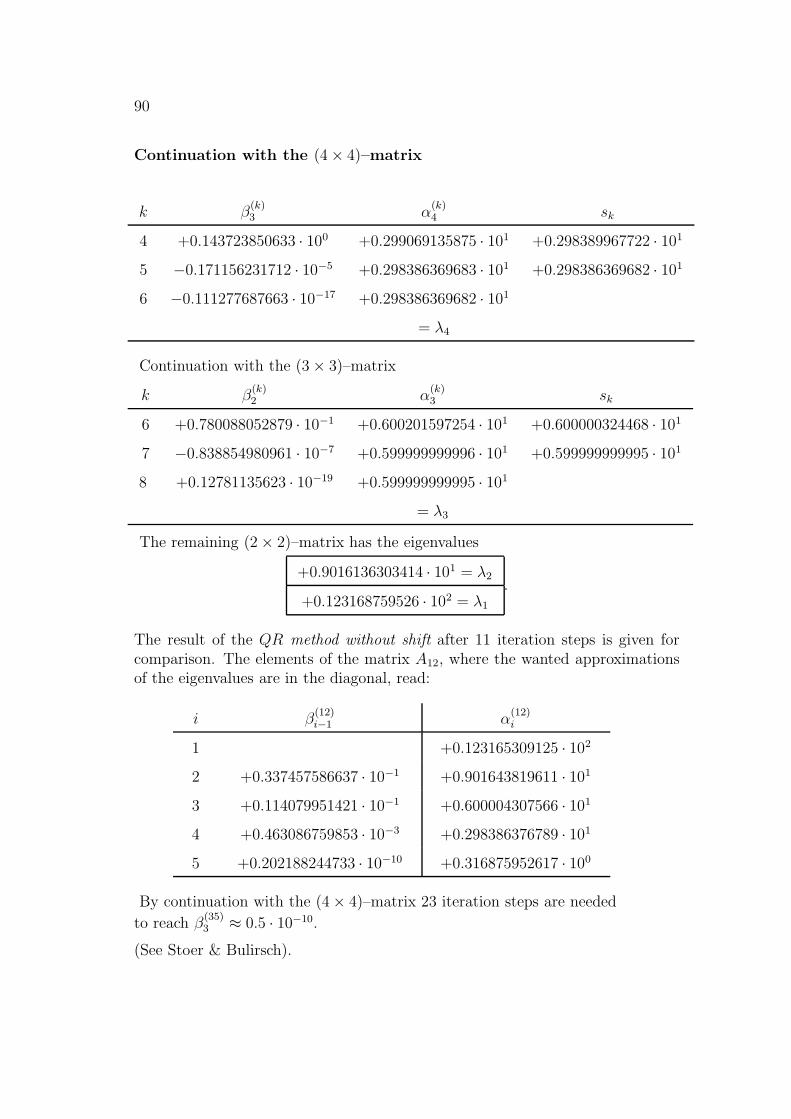
90
Continuation with the (4× 4)–matrix
k β(k)3 α
(k)4 sk
4 +0.143723850633 · 100 +0.299069135875 · 101 +0.298389967722 · 101
5 −0.171156231712 · 10−5 +0.298386369683 · 101 +0.298386369682 · 101
6 −0.111277687663 · 10−17 +0.298386369682 · 101
= λ4
Continuation with the (3× 3)–matrix
k β(k)2 α
(k)3 sk
6 +0.780088052879 · 10−1 +0.600201597254 · 101 +0.600000324468 · 101
7 −0.838854980961 · 10−7 +0.599999999996 · 101 +0.599999999995 · 101
8 +0.12781135623 · 10−19 +0.599999999995 · 101
= λ3
The remaining (2× 2)–matrix has the eigenvalues
+0.9016136303414 · 101 = λ2
+0.123168759526 · 102 = λ1
.
The result of the QR method without shift after 11 iteration steps is given forcomparison. The elements of the matrix A12, where the wanted approximationsof the eigenvalues are in the diagonal, read:
i β(12)i−1 α
(12)i
1 +0.123165309125 · 102
2 +0.337457586637 · 10−1 +0.901643819611 · 101
3 +0.114079951421 · 10−1 +0.600004307566 · 101
4 +0.463086759853 · 10−3 +0.298386376789 · 101
5 +0.202188244733 · 10−10 +0.316875952617 · 100
By continuation with the (4× 4)–matrix 23 iteration steps are needed
to reach β(35)3 ≈ 0.5 · 10−10.
(See Stoer & Bulirsch).
Chapter III
Numerical Treatment ofOrdinary Differential Equations
13 Basic Ideas
Initial Value Problem (IVP)
y′ = f(x, y), y(a) = y0, f : I × � → �, I := [a, b]
sector (rectangle), Lipschitz continuous
Wanted function u : I → �satisfying
1) u differentiable in I2) (x, u(x)) ∈ I × �
for all x ∈ I3) u′(x) = f(x, u(x)) for all x ∈ I and u(a) = y0
Then u is called solution of the IVP in the interval I.
Examplesy′ = qy, y(0) = 1 : u(x) = eqx
y′ = y2, y(0) = 1 : u(x) = 11−x (x 6= 1)
y′ = Ay, y(a) = y0 linear systemy′ = f(x, y), y(a) = y0 nonlinear system(f : I × � n → � n, solution u : I → � n)y′′ = f(x, y, y′) second order → reduction to a first order system
Theory existence, uniqueness, continuous dependence on theinitial value/right–hand side → well posedcontinuation of the solutionsolution theory (linear differential equation, Bernoulli differentialequation, exact differential equation, . . . )
91
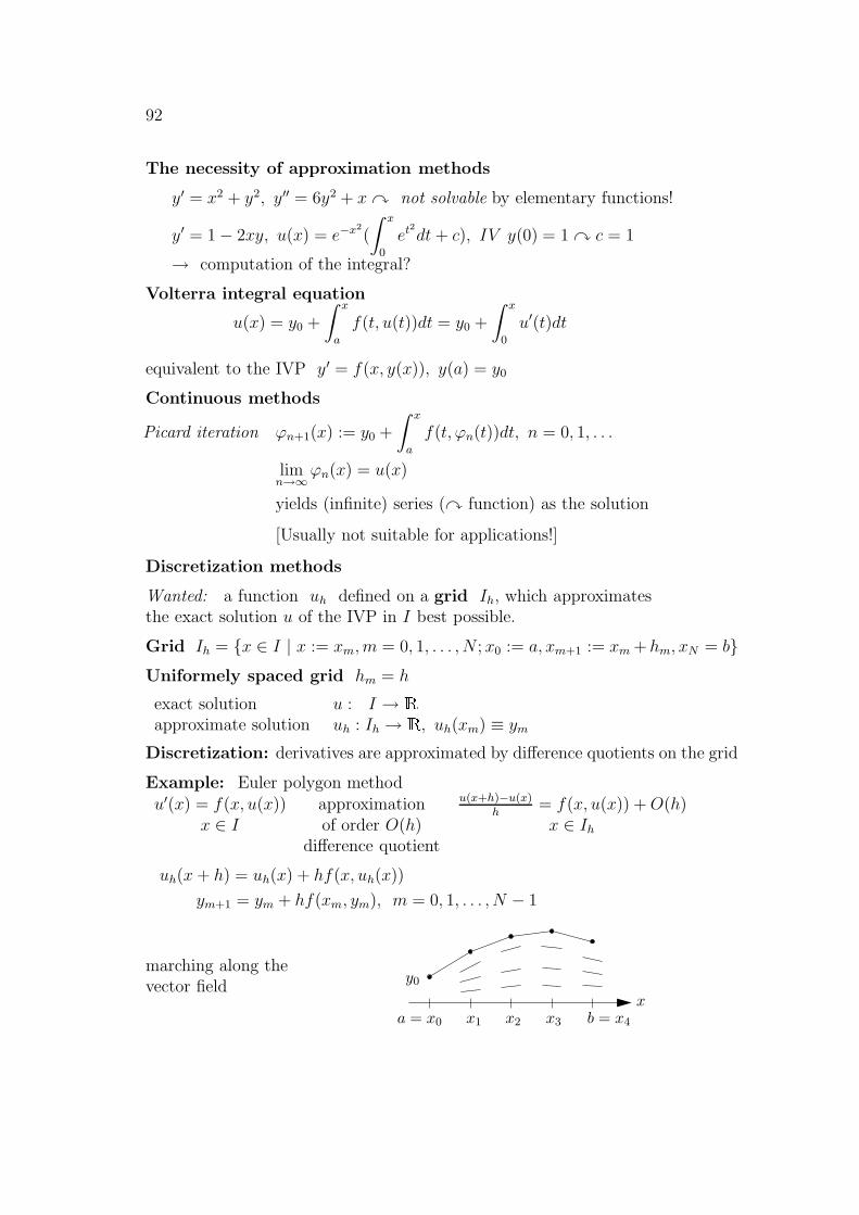
92
The necessity of approximation methods
y′ = x2 + y2, y′′ = 6y2 + xy not solvable by elementary functions!
y′ = 1− 2xy, u(x) = e−x2
(
∫ x
0
et2
dt + c), IV y(0) = 1 y c = 1
→ computation of the integral?
Volterra integral equation
u(x) = y0 +
∫ x
a
f(t, u(t))dt = y0 +
∫ x
0
u′(t)dt
equivalent to the IVP y′ = f(x, y(x)), y(a) = y0
Continuous methods
Picard iteration ϕn+1(x) := y0 +
∫ x
a
f(t, ϕn(t))dt, n = 0, 1, . . .
limn→∞
ϕn(x) = u(x)
yields (infinite) series (y function) as the solution
[Usually not suitable for applications!]
Discretization methods
Wanted: a function uh defined on a grid Ih, which approximatesthe exact solution u of the IVP in I best possible.
Grid Ih = {x ∈ I | x := xm, m = 0, 1, . . . , N ; x0 := a, xm+1 := xm + hm, xN = b}Uniformely spaced grid hm = h
exact solution u : I → �
approximate solution uh : Ih →�, uh(xm) ≡ ym
Discretization: derivatives are approximated by difference quotients on the grid
Example: Euler polygon methodu′(x) = f(x, u(x)) approximation u(x+h)−u(x)
h= f(x, u(x)) +O(h)
x ∈ I of order O(h) x ∈ Ihdifference quotient
uh(x + h) = uh(x) + hf(x, uh(x))
ym+1 = ym + hf(xm, ym), m = 0, 1, . . . , N − 1
marching along thevector field
PSfrag replacements
y0
a = x0 x1 x2 x3 b = x4
x
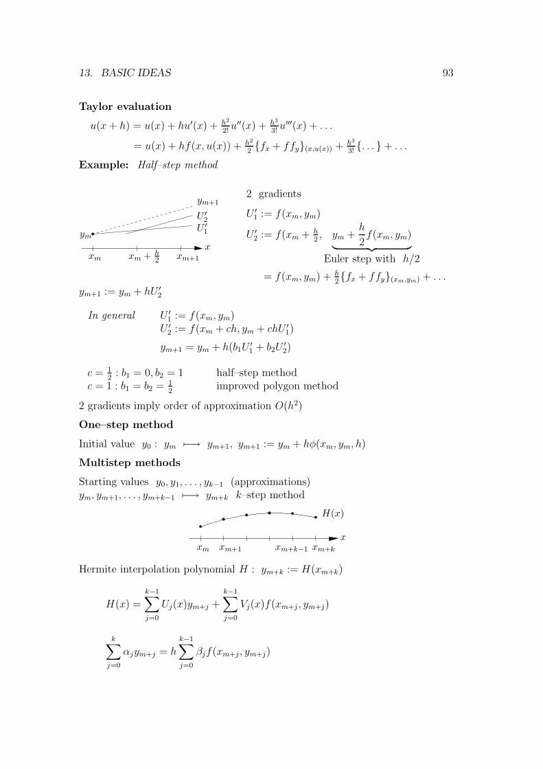
13. BASIC IDEAS 93
Taylor evaluation
u(x+ h) = u(x) + hu′(x) + h2
2!u′′(x) + h3
3!u′′′(x) + . . .
= u(x) + hf(x, u(x)) + h2
2{fx + ffy}(x,u(x)) + h3
3!{. . . }+ . . .
Example: Half–step method
PSfrag replacements
ym
xm xm + h2 xm+1
x
U ′1
U ′2
ym+12 gradients
U ′1 := f(xm, ym)
U ′2 := f(xm + h2, ym +
h
2f(xm, ym)
︸ ︷︷ ︸Euler step with h/2
= f(xm, ym) + h2{fx + ffy}(xm,ym) + . . .
ym+1 := ym + hU ′2
In general U ′1 := f(xm, ym)U ′2 := f(xm + ch, ym + chU ′1)
ym+1 = ym + h(b1U′1 + b2U
′2)
c = 12
: b1 = 0, b2 = 1 half–step methodc = 1 : b1 = b2 = 1
2improved polygon method
2 gradients imply order of approximation O(h2)
One–step method
Initial value y0 : ym 7−→ ym+1, ym+1 := ym + hφ(xm, ym, h)
Multistep methods
Starting values y0, y1, . . . , yk−1 (approximations)ym, ym+1, . . . , ym+k−1 7−→ ym+k k–step method
PSfrag replacements
xm xm+1 xm+k−1 xm+k
x
H(x)
Hermite interpolation polynomial H : ym+k := H(xm+k)
H(x) =
k−1∑
j=0
Uj(x)ym+j +
k−1∑
j=0
Vj(x)f(xm+j, ym+j)
k∑
j=0
αjym+j = hk−1∑
j=0
βjf(xm+j, ym+j)
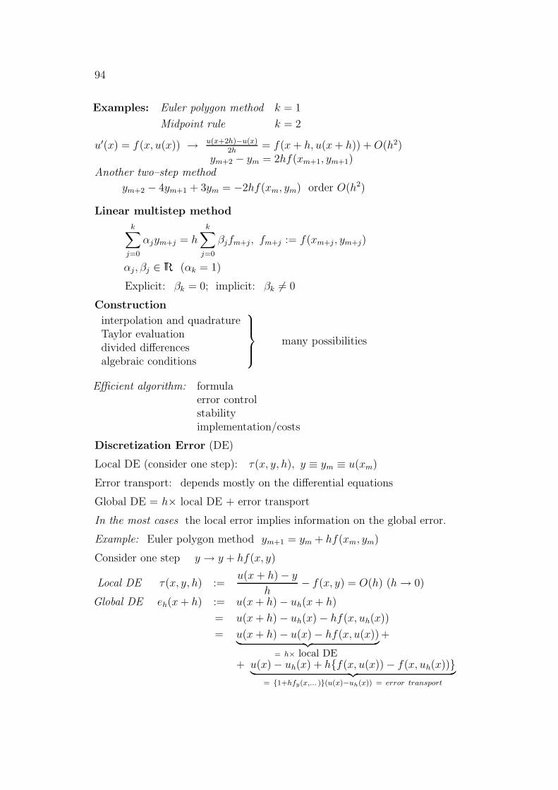
94
Examples: Euler polygon method k = 1
Midpoint rule k = 2
u′(x) = f(x, u(x)) → u(x+2h)−u(x)2h
= f(x+ h, u(x+ h)) +O(h2)ym+2 − ym = 2hf(xm+1, ym+1)
Another two–step method
ym+2 − 4ym+1 + 3ym = −2hf(xm, ym) order O(h2)
Linear multistep method
k∑
j=0
αjym+j = h
k∑
j=0
βjfm+j, fm+j := f(xm+j, ym+j)
αj, βj ∈�
(αk = 1)
Explicit: βk = 0; implicit: βk 6= 0
Construction
interpolation and quadratureTaylor evaluationdivided differencesalgebraic conditions
many possibilities
Efficient algorithm: formulaerror controlstabilityimplementation/costs
Discretization Error (DE)
Local DE (consider one step): τ(x, y, h), y ≡ ym ≡ u(xm)
Error transport: depends mostly on the differential equations
Global DE = h× local DE + error transport
In the most cases the local error implies information on the global error.
Example: Euler polygon method ym+1 = ym + hf(xm, ym)
Consider one step y → y + hf(x, y)
Local DE τ(x, y, h) :=u(x + h)− y
h− f(x, y) = O(h) (h→ 0)
Global DE eh(x+ h) := u(x+ h)− uh(x+ h)
= u(x+ h)− uh(x)− hf(x, uh(x))
= u(x+ h)− u(x)− hf(x, u(x))︸ ︷︷ ︸= h× local DE
+
+ u(x)− uh(x) + h{f(x, u(x))− f(x, uh(x))}︸ ︷︷ ︸= {1+hfy(x,... )}(u(x)−uh(x)) = error transport
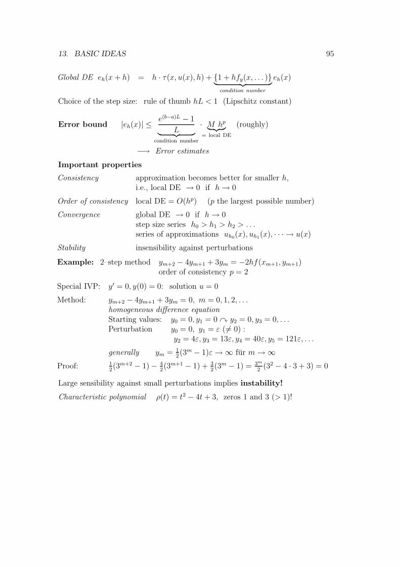
13. BASIC IDEAS 95
Global DE eh(x+ h) = h · τ(x, u(x), h) + {1 + hfy(x, . . . )}︸ ︷︷ ︸condition number
eh(x)
Choice of the step size: rule of thumb hL < 1 (Lipschitz constant)
Error bound |eh(x)| ≤ e(b−a)L − 1
L︸ ︷︷ ︸condition number
· M hp︸ ︷︷ ︸= local DE
(roughly)
−→ Error estimates
Important properties
Consistency approximation becomes better for smaller h,i.e., local DE → 0 if h→ 0
Order of consistency local DE = O(hp) (p the largest possible number)
Convergence global DE → 0 if h→ 0step size series h0 > h1 > h2 > . . .series of approximations uh0(x), uh1(x), · · · → u(x)
Stability insensibility against perturbations
Example: 2–step method ym+2 − 4ym+1 + 3ym = −2hf(xm+1, ym+1)order of consistency p = 2
Special IVP: y′ = 0, y(0) = 0: solution u = 0
Method: ym+2 − 4ym+1 + 3ym = 0, m = 0, 1, 2, . . .homogeneous difference equationStarting values: y0 = 0, y1 = 0 y y2 = 0, y3 = 0, . . .Perturbation y0 = 0, y1 = ε (6= 0) :
y2 = 4ε, y3 = 13ε, y4 = 40ε, y5 = 121ε, . . .
generally ym = 12(3m − 1)ε→∞ fur m→∞
Proof: 12(3m+2 − 1)− 4
2(3m+1 − 1) + 3
2(3m − 1) = 3m
2(32 − 4 · 3 + 3) = 0
Large sensibility against small perturbations implies instability!
Characteristic polynomial ρ(t) = t2 − 4t+ 3, zeros 1 and 3 (> 1)!
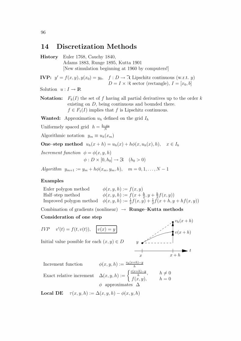
96
14 Discretization Methods
History Euler 1768, Cauchy 1840,Adams 1883, Runge 1895, Kutta 1901[New stimulation beginning at 1960 by computers!]
IVP: y′ = f(x, y), y(x0) = y0, f : D → �Lipschitz continuous (w.r.t. y)
D = I × �sector (rectangle), I = [x0, b]
Solution u : I → �
Notation: Fk(I) the set of f having all partial derivatives up to the order kexisting on D, being continuous and bounded there.f ∈ F1(I) implies that f is Lipschitz continuous.
Wanted: Approximation uh defined on the grid Ih
Uniformely spaced grid h = b−x0
N
Algorithmic notation ym ≡ uh(xm)
One–step method uh(x + h) = uh(x) + hφ(x, uh(x), h), x ∈ IhIncrement function φ = φ(x, y, h)
φ : D × [0, h0]→ �(h0 > 0)
Algorithm ym+1 := ym + hφ(xm, ym, h), m = 0, 1, . . . , N − 1
Examples
Euler polygon method φ(x, y, h) := f(x, y)Half–step method φ(x, y, h) := f(x+ h
2, y + h
2f(x, y))
Improved polygon method φ(x, y, h) := 12f(x, y) + 1
2f(x + h, y + hf(x, y))
Combination of gradients (nonlinear) → Runge–Kutta methods
Consideration of one step
IVP v′(t) = f(t, v(t)), v(x) = y
Initial value possible for each (x, y) ∈ D
PSfrag replacements
x x+ ht
y
v(x+ h)
vh(x+ h)
Increment function φ(x, y, h) := vh(x+h)−yh
Exact relative increment ∆(x, y, h) :=
{v(x+h)−y
h, h 6= 0
f(x, y), h = 0φ approximates ∆
Local DE τ(x, y, h) := ∆(x, y, h)− φ(x, y, h)

14. DISCRETIZATION METHODS 97
Consistency τ(x, y, h) = O(h) (h→ 0) f.a. (x, y) ∈ D and f.a. f ∈ F1(I)
Definition: A one–step method has order of consistency p, if it satisfiesτ(x, y, h) = O(hp) (h→ 0) f.a. (x, y) ∈ D and f.a. f ∈ Fp(I).
Euler polygon method τ(x, y, h) =
{v(x+h)−y
h− f(x, y), h 6= 00, h = 0
Taylor τ(x, y, h) = 1h{v(x) + h v′(x) + h2
2v′′(x) + · · · − y} − f(x, y)
= h2v′′(x) + · · · = O(h) (h→ 0) f.a. (x, y) ∈ D
Half–step method τ(x, y, h) = O(h2)
∆(x, y, h) = v(x+h)−yh
= v′(x)+ h2v′′(x)+· · · = f(x, y)+ h
2{fx+ffy}(x,y)+O(h2)
φ(x, y, h) = f(x+ 12h, y + 1
2hf(x, y)) = f(x, y) + h
2{fx + ffy}(x,y) +O(h2)
implies order of consistency p = 2
Linear multistep methods
k∑
j=0
αjym+j = h
h∑
j=0
βjfm+j, fm+j := f(xm+j, ym+j), y′m+j ≡ fm+k
Real parameters α0, . . . , αk, β0, . . . , βk; αk = 1, |α0|+ |β0| > 0(the reduction to k − 1 steps is not possible)
Explicit: βk = 0
Implicit: βk 6= 0 iteration y Predictor–Corrector method
Abbreviation
Characteristic polynomials ρ(ξ) :=k∑
j=0
αjξj, σ(ξ) :=
k∑
j=0
βjξj
Shift operator E (j ∈ � ) : Eym := ym+1
Ejym := ym+j
∣∣∣∣Eu(x) := u(x + h)Eju(x) := u(x+ jh)
Linear k–step method (ρ, σ) : ρ(E)ym = hσ(E)y′m
Consideration of one step (without error transport):
Exact values u(x), u(x+ h), . . . , u(x+ (k − 1)h) → uh(x + kh)
98
Linear difference operator Lh : C1 → C
Lh(u(·)) :=k∑j=0
αju(·+ jh)− hk∑j=0
βju′(·+ jh)
= u(·+ kh)− {−k−1∑
j=0
αju(·+ jh) + h
k∑
j=0
βju′(·+ jh)
︸ ︷︷ ︸=:uh(·+kh)
}
Taylor evaluation f ∈ Fp(I), i.e. u ∈ Cp+1(I)
u(x+ jh) = u(x) + jhu′(x) + · · ·+ jp
p!hpu(p)(x) +O(hp+1) (h→ 0)
u′(x + jh) = u′(x) + jhu′′(x) + · · ·+ jp−1
(p−1)!hp−1u(p)(x) +O(hp) (h→ 0)
Lh(u(x)) = C0u(x) + C1hu′(x) + · · ·+ Cph
pu(p)(x) +O(hp+1) (h→ 0)
with C0 =k∑j=0
αj, Cν =k∑j=0
(αjjν
ν!− βj jν−1
(ν−1)!), ν = 1, . . . , p
Local discretization error
IVP (x, y) ∈ D : v′(t) = f(t, v(t)), v(x) = y, solution v
Local DE τ(x, y, h) := 1hρ(E)v(x)− σ(E)v′(x) = 1
hLh(v(x))
To emphasize the step number k use τk := τk(x, y, h)
Definition A linear multistep method is called consistent, if
τ(x, y, h) = O(h) (h→ 0) f.a. (x, y) ∈ D and f.a. f ∈ F1(I).
Condition of consistency C0 = C1 = 0, i.e., ρ(1) = 0, ρ′(1) = σ(1)
Definition A linear multistep method has order of consistency p, if
τ(x, y, h) = O(hp) (h→ 0) f.a. (x, y) ∈ D and f.a. f ∈ Fp(I).
Order of consistency p : C0 = · · · = Cp = 0 y linear system
0 :∑k
αj = 0
1 :k∑j=0
(αj · j − βj) = 0
ν :k∑j=0
(αjjν
ν:− βj jν−1
(ν−1)!) = 0, ν = 2, . . . , p (αk = 1)
14. DISCRETIZATION METHODS 99
Number of coefficients: 2k + 1Number of equations: p+ 1
}⇒
maximal order of consistency p∗(k) = 2k
Examples
ym+2 − ym = 2hfm+1, p = 2
ym+2 − 4ym+1 + 3ym = −2hfm, p = 2
ym+2 − ym+1 = 12h(3fm+1 − fm), p = 2
ym+1 − ym = 12h(fm + fm+1), k = 1, p = 2 (trapezoidal rule)
Consistent starting values y0, y1, . . . , yk−1
IVP v′(t) = f(t, v(t)), v(x) = y
Definition The starting values yh0 , . . . , yhk−1 w.r.t. x, x + h, . . . , x+ (k − 1)h
are called consistent, if max0≤j≤k−1
|yhj − v(x+ jh)| = O(h) (h→ 0) f.a. (x, y) ∈ D.
RemarksLarge approximation errors of the starting values cannot be repaired again!The starting values must have the same approximation order as the chosendiscretization method!
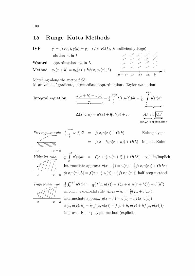
100
15 Runge–Kutta Methods
IVP y′ = f(x, y), y(a) = y0 (f ∈ Fk(I), k sufficiently large)
solution u in I
Wanted approximation uh in Ih
Method uh(x + h) = uh(x) + hφ(x, uh(x), h)
PSfrag replacements
a = x0 x1 x2 x3 bx
Marching along the vector field:Mean value of gradients, intermediate approximations, Taylor evaluation
Integral equationu(x+ h)− u(x)
h︸ ︷︷ ︸= 1
h
x+h∫x
f(t, u(t))dt = 1h
x+h∫
x
u′(t)dt
︸ ︷︷ ︸
∆(x, y, h) = u′(x) + h2u′′(x) + . . . AP y QF
︸ ︷︷ ︸φ(x,y,h)+approx.error
Rectangular rule
PSfrag replacements
x x+ h
1h
x+h∫x
u′(t)dt = f(x, u(x)) +O(h) Euler polygon
= f(x + h, u(x+ h)) +O(h) implicit Euler
Midpoint rule
PSfrag replacements
x x+ h
1h
x+h∫x
u′(t)dt = f(x+ h2, u(x+ h
2)) +O(h2) explicit/implicit
Intermediate approx.: u(x+ h2) = u(x) + h
2f(x, u(x)) +O(h2)
φ(x, u(x), h) = f(x+ h2, u(x) + h
2f(x, u(x))) half–step method
Trapezoidal rule
PSfrag replacements
x x+ h
1h
∫ x+h
xu′(t)dt = 1
2{f(x, u(x)) + f(x + h, u(x+ h))}+O(h2)
implicit trapezoidal rule ym+1 − ym = h2(fm + fm+1)
intermediate approx.: u(x+ h) = u(x) + hf(x, u(x))
φ(x, u(x), h) = 12{f(x, u(x)) + f(x + h, u(x) + hf(x, u(x)))}
improved Euler polygon method (explicit)
15. RUNGE–KUTTA METHODS 101
Algorithm: Gradients by recurrence (2–stage method)
U ′1 := f(xm, ym)
U2 := ym + ha21U′1
U ′2 := f(xm + c2h, U2)
ym+1 := ym + h(b1U′1 + b2U
′2)
scheme
0 0 0 b1
c2 a21 0 b2
Coefficients: a21 = c2 = 12, b1 = 0, b2 = 1 and a21 = c2 = 1, b1 = b2 = 1
2
Quadrature formula: Nodes (0, c2), weights (b1, b2)
Pure quadrature formula if y′ = f(x)
Taylor evaluation
∆(x, u(x), h) = u′(x) + h2u′′(x) + h2
3!u′′′(x) + . . . (u(x) = y)
= f(x, y) + h2{fx + ffy}(x,y) + h2
3!{. . . }+ . . .
U ′1 = f(x, y)
U ′2 = f(x+ c2h, y + ha21f(x, y)) = f(x, y) + {c2fx + a21ffy}(x,y) + . . .
φ(x, u(x), h) = b1U′1 + b2U
′2
= (b1 + b2)f(x, y) + hb2{c2fx + a21ffy}(x,y) + . . .
τ(x, u(x), h) = ∆(x, u(x), h)− φ(x, u(x), h)
= (1− b1 − b2)︸ ︷︷ ︸=0
f(x, y) + h[(1
2− b2c2
︸ ︷︷ ︸=0
)fx + (1
2− b2a21
︸ ︷︷ ︸=0
)ffy](x,y) + . . .
general assumption x c2 = a21 (b2 6= 0)
Order of consistency p = 1 b1 + b2 = 1 (Σ weights = 1)
p = 2 b2c2 = 12, c2 = a21
Solution: c2 6= 0, b2 6= 0 (otherwise only one stage)
b1 = 1− 12c2, b2 = 1
2c21 independent parameter s = p = 2
half–step method: c2 = 12, improved Euler method: c2 = 1
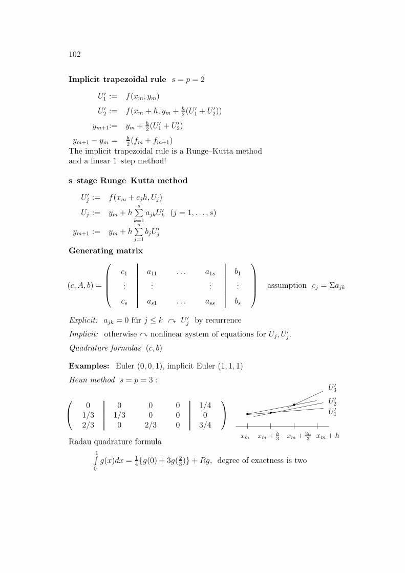
102
Implicit trapezoidal rule s = p = 2
U ′1 := f(xm, ym)
U ′2 := f(xm + h, ym + h2(U ′1 + U ′2))
ym+1:= ym + h2(U ′1 + U ′2)
ym+1 − ym = h2(fm + fm+1)
The implicit trapezoidal rule is a Runge–Kutta methodand a linear 1–step method!
s–stage Runge–Kutta method
U ′j := f(xm + cjh, Uj)
Uj := ym + hs∑
k=1
ajkU′k (j = 1, . . . , s)
ym+1 := ym + hs∑j=1
bjU′j
Generating matrix
(c, A, b) =
c1 a11 . . . a1s b1
......
......
cs as1 . . . ass bs
assumption cj = Σajk
Explicit: ajk = 0 fur j ≤ k y U ′j by recurrence
Implicit: otherwise y nonlinear system of equations for Uj, U′j.
Quadrature formulas (c, b)
Examples: Euler (0, 0, 1), implicit Euler (1, 1, 1)
Heun method s = p = 3 :
0 0 0 0 1/41/3 1/3 0 0 02/3 0 2/3 0 3/4
PSfrag replacements
xm xm + h3 xm + 2h
3 xm + h
U ′1
U ′2
U ′3
Radau quadrature formula
1∫0
g(x)dx = 14{g(0) + 3g( 2
3)}+Rg, degree of exactness is two
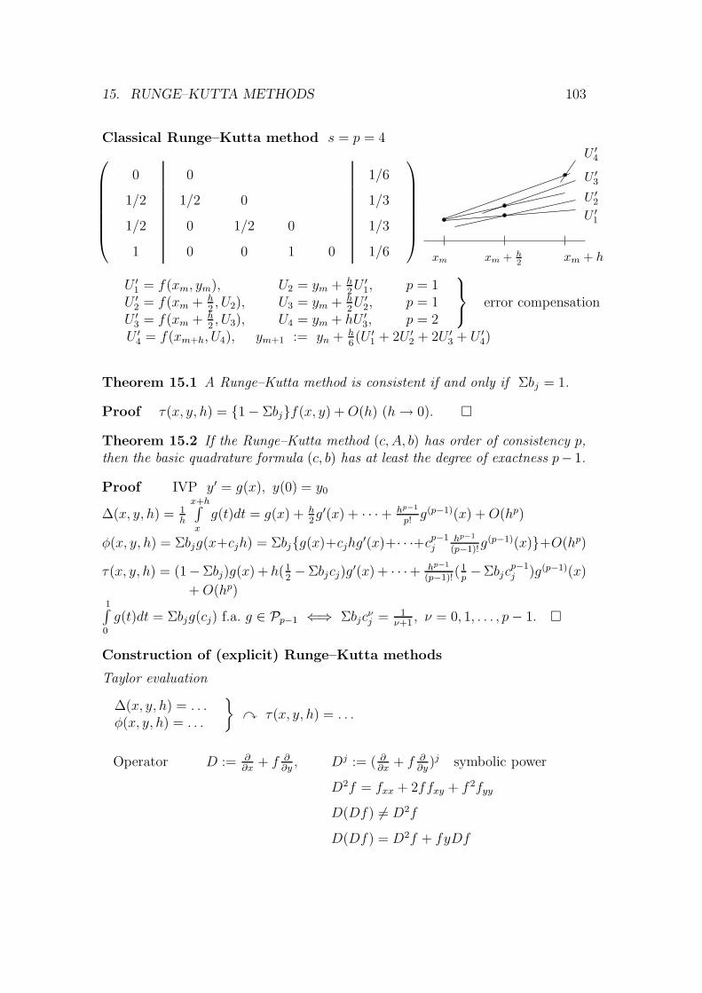
15. RUNGE–KUTTA METHODS 103
Classical Runge–Kutta method s = p = 4
0 0 1/6
1/2 1/2 0 1/3
1/2 0 1/2 0 1/3
1 0 0 1 0 1/6
PSfrag replacements
xm xm + h2 xm + h
U ′1
U ′2
U ′3
U ′4
U ′1 = f(xm, ym), U2 = ym + h2U ′1, p = 1
U ′2 = f(xm + h2, U2), U3 = ym + h
2U ′2, p = 1
U ′3 = f(xm + h2, U3), U4 = ym + hU ′3, p = 2
error compensation
U ′4 = f(xm+h, U4), ym+1 := yn + h6(U ′1 + 2U ′2 + 2U ′3 + U ′4)
Theorem 15.1 A Runge–Kutta method is consistent if and only if Σbj = 1.
Proof τ(x, y, h) = {1− Σbj}f(x, y) +O(h) (h→ 0). �
Theorem 15.2 If the Runge–Kutta method (c, A, b) has order of consistency p,then the basic quadrature formula (c, b) has at least the degree of exactness p− 1.
Proof IVP y′ = g(x), y(0) = y0
∆(x, y, h) = 1h
x+h∫x
g(t)dt = g(x) + h2g′(x) + · · ·+ hp−1
p!g(p−1)(x) +O(hp)
φ(x, y, h) = Σbjg(x+cjh) = Σbj{g(x)+cjhg′(x)+· · ·+cp−1
jhp−1
(p−1)!g(p−1)(x)}+O(hp)
τ(x, y, h) = (1−Σbj)g(x) + h(12−Σbjcj)g
′(x) + · · ·+ hp−1
(p−1)!(1p−Σbjc
p−1j )g(p−1)(x)
+O(hp)1∫0
g(t)dt = Σbjg(cj) f.a. g ∈ Pp−1 ⇐⇒ Σbjcνj = 1
ν+1, ν = 0, 1, . . . , p− 1. �
Construction of (explicit) Runge–Kutta methods
Taylor evaluation
∆(x, y, h) = . . .φ(x, y, h) = . . .
}y τ(x, y, h) = . . .
Operator D := ∂∂x
+ f ∂∂y, Dj := ( ∂
∂x+ f ∂
∂y)j symbolic power
D2f = fxx + 2ffxy + f 2fyy
D(Df) 6= D2f
D(Df) = D2f + fyDf
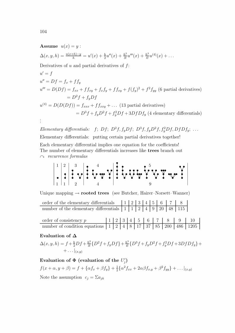
104
Assume u(x) = y :
∆(x, y, h) = u(x+h)−yh
= u′(x) + h2u′′(x) + h2
3!u′′′(x) + h3
4!u(4)(x) + . . .
Derivatives of u and partial derivatives of f :
u′ = f
u′′ = Df = fx + ffy
u′′′ = D(Df) = fxx + ffxy + fxfy + ffxy + f(fy)2 + f 2fyy (6 partial derivatives)
= D2f + fyDf
u(4) = D(D(Df)) = fxxx + ffxxy + . . . (13 partial derivatives)
= D3f + fyD2f + f 2
yDf + 3DfDfy (4 elementary differentials)...
Elementary differentials: f ; Df ; D2f, fyDf ; D3f, fyD2f, f 2
yDf,DfDfy; . . .
Elementary differentials: putting certain partial derivatives together!
Each elementary differential implies one equation for the coefficients!The number of elementary differentials increases like trees branch outy recurrence formulas
PSfrag replacements
1 2 3 4 5
1 1 2 4 9
Unique mapping → rooted trees (see Butcher, Hairer–Norsett–Wanner)
order of the elementary differentials 1 2 3 4 5 6 7 8number of the elementary differentials 1 1 2 4 9 20 48 115
order of consistency p 1 2 3 4 5 6 7 8 9 10number of condition equations 1 2 4 8 17 37 85 200 486 1205
Evaluation of ∆
∆(x, y, h) = f+ h2Df+ h2
3!{D2f+fyDf}+ h3
4!{D3f+fyD
2f+f 2yDf+3DfDfy}+
+ . . . |(x,y)
Evaluation of Φ (evaluation of the U ′j)
f(x+ α, y + β) = f + {αfx + βfy}+ 12{α2fxx + 2αβfx,y + β2fyy}+ . . . |(x,y)
Note the assumption cj = Σajk
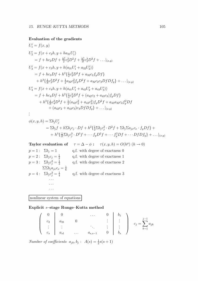
15. RUNGE–KUTTA METHODS 105
Evaluation of the gradients
U ′1 = f(x, y)
U ′2 = f(x+ c2h, y + ha21U′1)
= f + hc2Df + h2
2c2
2D2f + h3
3!c3
2D3f + . . . |(x,y)
U ′3 = f(x+ c3h, y + h(a31U′1 + a32U
′2))
= f + hc3Df + h2{12c2
3D2f + a32c2fyDf}
+ h3{ 13!c3
3D3f + 1
2a32c
22fyD
2f + a32c2c3DfDfy}+ . . . |(x,y)
U ′4 = f(x+ c4h, y + h(a41U′1 + a42U
′2 + a43U
′3))
= f + hc4Df + h2{12c2
4D2f + (a42c2 + a43c3)fyDf}
+ h3{ 13!c3
4D3f + 1
2(a42c
22 + a43c
23)fyD
2f + a43a32c2f2yDf
+ (a42c2 + a43c3)c4DfDfy}+ . . . |(x,y)
...
φ(x, y, h) = ΣbjU′j
= Σbjf + hΣbjcj ·Df + h2{12Σbjc
2j ·D2f + ΣbjΣajνcν · fyDf}+
+ h3{ 13!
Σbjc3j ·D3f + · · · fyD2f + · · · f 2
yDf + · · ·DfDfy}+ . . . |(x,y)
Taylor evaluation of τ = ∆− φ : τ(x, y, h) = O(hp) (h→ 0)
p = 1 : Σbj = 1 q.f. with degree of exactness 0
p = 2 : Σbjcj = 12
q.f. with degree of exactness 1
p = 3 : Σbjc2j = 1
3q.f. with degree of exactness 2
ΣΣbjajνcν = 16
p = 4 : Σbjc3j = 1
4q.f. with degree of exactness 3
. . .
. . .
. . .
nonlinear system of equations
Explicit s–stage Runge–Kutta method
0 0 . . . 0 b1
c2 a21 0...
......
.... . .
......
cs as1 . . . as,s−1 0 bs
cj =
j−1∑
k=1
ajk
Number of coefficients ajk, bj : A(s) = 12s(s+ 1)
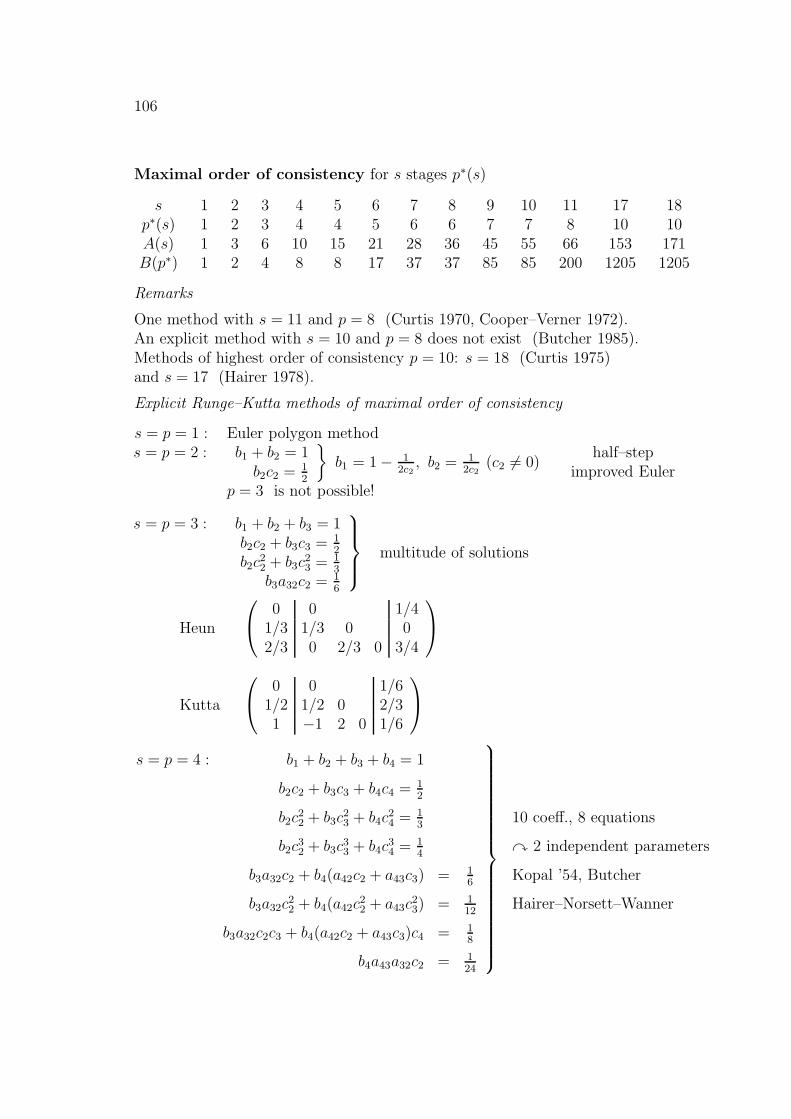
106
Maximal order of consistency for s stages p∗(s)
s 1 2 3 4 5 6 7 8 9 10 11 17 18p∗(s) 1 2 3 4 4 5 6 6 7 7 8 10 10A(s) 1 3 6 10 15 21 28 36 45 55 66 153 171B(p∗) 1 2 4 8 8 17 37 37 85 85 200 1205 1205
Remarks
One method with s = 11 and p = 8 (Curtis 1970, Cooper–Verner 1972).An explicit method with s = 10 and p = 8 does not exist (Butcher 1985).Methods of highest order of consistency p = 10: s = 18 (Curtis 1975)and s = 17 (Hairer 1978).
Explicit Runge–Kutta methods of maximal order of consistency
s = p = 1 : Euler polygon methods = p = 2 : b1 + b2 = 1
b2c2 = 12
}b1 = 1− 1
2c2, b2 = 1
2c2(c2 6= 0)
half–stepimproved Euler
p = 3 is not possible!
s = p = 3 : b1 + b2 + b3 = 1b2c2 + b3c3 = 1
2
b2c22 + b3c
23 = 1
3
b3a32c2 = 16
multitude of solutions
Heun
0 0 1/41/3 1/3 0 02/3 0 2/3 0 3/4
Kutta
0 0 1/61/2 1/2 0 2/31 −1 2 0 1/6
s = p = 4 : b1 + b2 + b3 + b4 = 1
b2c2 + b3c3 + b4c4 = 12
b2c22 + b3c
23 + b4c
24 = 1
3
b2c32 + b3c
33 + b4c
34 = 1
4
b3a32c2 + b4(a42c2 + a43c3) = 16
b3a32c22 + b4(a42c
22 + a43c
23) = 1
12
b3a32c2c3 + b4(a42c2 + a43c3)c4 = 18
b4a43a32c2 = 124
10 coeff., 8 equations
y 2 independent parameters
Kopal ’54, Butcher
Hairer–Norsett–Wanner
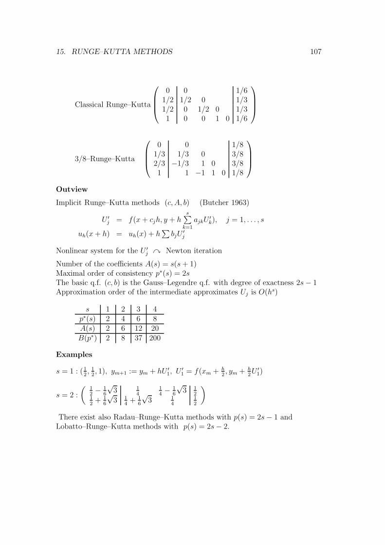
15. RUNGE–KUTTA METHODS 107
Classical Runge–Kutta
0 0 1/61/2 1/2 0 1/31/2 0 1/2 0 1/31 0 0 1 0 1/6
3/8–Runge–Kutta
0 0 1/81/3 1/3 0 3/82/3 −1/3 1 0 3/81 1 −1 1 0 1/8
Outview
Implicit Runge–Kutta methods (c, A, b) (Butcher 1963)
U ′j = f(x+ cjh, y + hs∑
k=1
ajkU′k), j = 1, . . . , s
uh(x+ h) = uh(x) + h∑bjU
′j
Nonlinear system for the U ′j y Newton iteration
Number of the coefficients A(s) = s(s+ 1)Maximal order of consistency p∗(s) = 2sThe basic q.f. (c, b) is the Gauss–Legendre q.f. with degree of exactness 2s− 1Approximation order of the intermediate approximates Uj is O(hs)
s 1 2 3 4p∗(s) 2 4 6 8A(s) 2 6 12 20B(p∗) 2 8 37 200
Examples
s = 1 : (12, 1
2, 1), ym+1 := ym + hU ′1, U
′1 = f(xm + h
2, ym + h
2U ′1)
s = 2 :
(12− 1
6
√3 1
414− 1
6
√3 1
212
+ 16
√3 1
4+ 1
6
√3 1
412
)
There exist also Radau–Runge–Kutta methods with p(s) = 2s− 1 andLobatto–Runge–Kutta methods with p(s) = 2s− 2.

108
Tree theory
Graphic representation of the elementary differential (or order conditions)
A tree consists of vertices and branches; the lowest vertex is called root;the vertices are noted by indices and the set of vertices is given by {j, k, `, . . .};the branches represent the mappings k → j, `→ j, . . . (downward);the order of the tree is the number of elements of the set of vertices.
PSfrag replacementsk l
j
set of vertices {j, k, `}, root jset of branches {k → j, `→ j}2 branches from the first floor to the rootorder of the tree is 3 (=number of vertices)
Equivalent trees
1) the same order2) equivalent set of branches
the same order3 branches from the first floor to the root1 branch from the second to the first floor(no matter to which vertex)
Definition by recurrence: order q → q + 11) root remains root2) attach to an arbitrary vertex exactly one additional branch upward,
i.e., the new tree has one more vertex3) do it for each vertex4) equivalent trees are classified as one tree
PSfrag replacements1 2 3 4
5
f Df D2f fyDf D3f DfDfy fyD2f f2
yDf
D4f
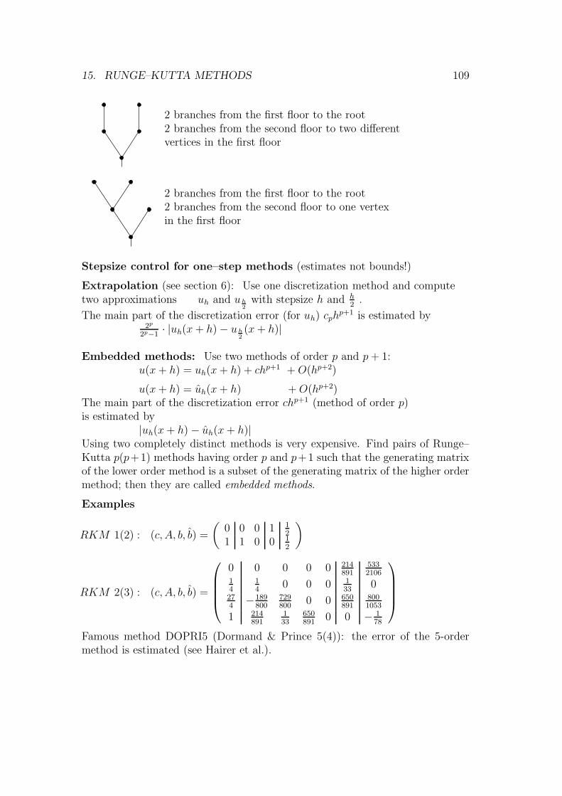
15. RUNGE–KUTTA METHODS 109
2 branches from the first floor to the root2 branches from the second floor to two differentvertices in the first floor
2 branches from the first floor to the root2 branches from the second floor to one vertexin the first floor
Stepsize control for one–step methods (estimates not bounds!)
Extrapolation (see section 6): Use one discretization method and computetwo approximations uh and uh
2with stepsize h and h
2.
The main part of the discretization error (for uh) cphp+1 is estimated by
2p
2p−1· |uh(x + h)− uh
2(x+ h)|
Embedded methods: Use two methods of order p and p+ 1:u(x+ h) = uh(x+ h) + chp+1 +O(hp+2)
u(x+ h) = uh(x+ h) +O(hp+2)The main part of the discretization error chp+1 (method of order p)is estimated by
|uh(x+ h)− uh(x+ h)|Using two completely distinct methods is very expensive. Find pairs of Runge–Kutta p(p+1) methods having order p and p+1 such that the generating matrixof the lower order method is a subset of the generating matrix of the higher ordermethod; then they are called embedded methods.
Examples
RKM 1(2) : (c, A, b, b) =
(0 0 0 1 1
2
1 1 0 0 12
)
RKM 2(3) : (c, A, b, b) =
0 0 0 0 0 214891
5332106
14
14
0 0 0 133
0274−189
800729800
0 0 650891
8001053
1 214891
133
650891
0 0 − 178
Famous method DOPRI5 (Dormand & Prince 5(4)): the error of the 5-ordermethod is estimated (see Hairer et al.).
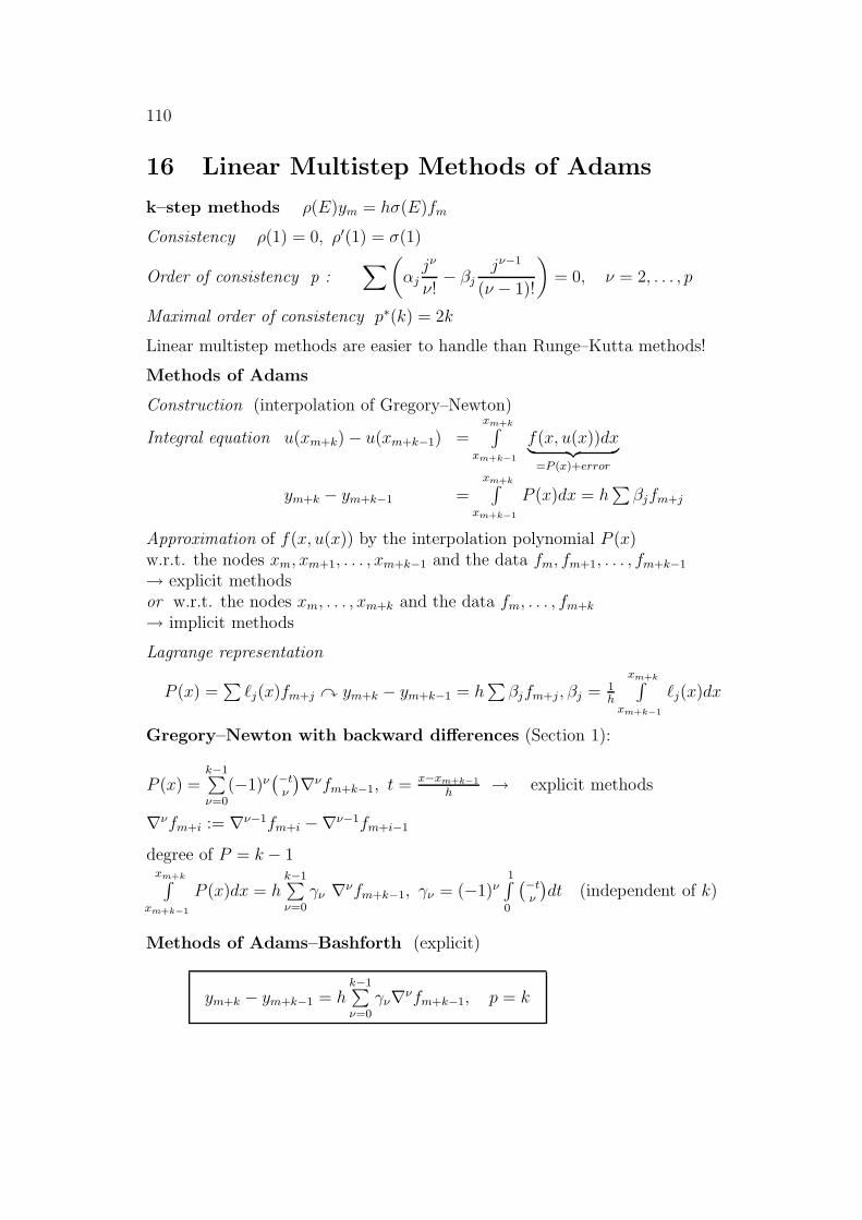
110
16 Linear Multistep Methods of Adams
k–step methods ρ(E)ym = hσ(E)fm
Consistency ρ(1) = 0, ρ′(1) = σ(1)
Order of consistency p :∑(
αjjν
ν!− βj
jν−1
(ν − 1)!
)= 0, ν = 2, . . . , p
Maximal order of consistency p∗(k) = 2k
Linear multistep methods are easier to handle than Runge–Kutta methods!
Methods of Adams
Construction (interpolation of Gregory–Newton)
Integral equation u(xm+k)− u(xm+k−1) =xm+k∫
xm+k−1
f(x, u(x))dx︸ ︷︷ ︸=P (x)+error
ym+k − ym+k−1 =xm+k∫
xm+k−1
P (x)dx = h∑βjfm+j
Approximation of f(x, u(x)) by the interpolation polynomial P (x)w.r.t. the nodes xm, xm+1, . . . , xm+k−1 and the data fm, fm+1, . . . , fm+k−1
→ explicit methodsor w.r.t. the nodes xm, . . . , xm+k and the data fm, . . . , fm+k
→ implicit methods
Lagrange representation
P (x) =∑`j(x)fm+j y ym+k − ym+k−1 = h
∑βjfm+j, βj = 1
h
xm+k∫xm+k−1
`j(x)dx
Gregory–Newton with backward differences (Section 1):
P (x) =k−1∑ν=0
(−1)ν(−tν
)∇νfm+k−1, t = x−xm+k−1
h→ explicit methods
∇νfm+i := ∇ν−1fm+i −∇ν−1fm+i−1
degree of P = k − 1xm+k∫
xm+k−1
P (x)dx = hk−1∑ν=0
γν ∇νfm+k−1, γν = (−1)ν1∫
0
(−tν
)dt (independent of k)
Methods of Adams–Bashforth (explicit)
ym+k − ym+k−1 = hk−1∑ν=0
γν∇νfm+k−1, p = k
16. LINEAR MULTISTEP METHODS OF ADAMS 111
Coefficients γν by recurrence relation
γν + 12γν−1 + 1
3γν−2 + · · ·+ 1
ν+1γ0 = 1, ν = 0, 1, 2, . . .
ν 0 1 2 3 4
γν 1 12
512
38
251720
{γν} = {0.5, 0.42, 0.38, 0.35, . . . } monotone decreasing
Examples
k = p = 2 : ym+2 − ym+1 = h(fm+1 + 12∇fm+1)
= h2(3fm+1 − fm)
k = p = 3 : ym+3 − ym+2 = h(fm+2 + 1
2∇fm+2
)+ 5
12h∇2fm+2
= h12
(23fm+2 − 16fm+1 + 5fm)
Local discretization error τ
k–step method: u′ = f(t, u(t)), u(x) = y → τ(x, y, h), τk := τ(xm, ym, h)
dm+k := h× τk =
xm+k∫
xm+k−1
{f(x, u(x))− P (x)}︸ ︷︷ ︸interpolation error
dx
f(x, u(x))︸ ︷︷ ︸−P (x) = 1k!u(k+1)(ξ(x)) (x− xm) . . . (x− xm+k−1)︸ ︷︷ ︸
= u′(x) no change of sign in (xm+k−1, xm+k)
Substitution t =x−xm+k−1
hy 1
hk1k!
(x− xm) . . . (x− xm+k−1) = (−1)k(−tk
)
y γk = (−1)k1∫
0
(−tk
)dt
Theorem 16.1 The Adams–Bashforth methods have the followingrepresentation and estimate of the local discretization error (main part):
dm+k = hk+1 γk u(k+1)(ξ), xm < ξ < xm+k−1
dm+k = h γk ∇k fm+k−1 +O(hk+2)

112
Error estimate and increasing the order of consistency
ym+k−ym+k−1 = h
k−1∑
ν=0
γν∇νfm+k−1
︸ ︷︷ ︸p=k
+ hγk∇kfm+k−1︸ ︷︷ ︸≈dm+k
︸ ︷︷ ︸p=k+1
+hγk+1∇k+1fm+k−1
︸ ︷︷ ︸p=k+2 (k+2)−step method
+ . . .
Difference scheme (Section 1)
xm−2 ∇◦fm−2 . . . . . . . . . ∇k−1fm+k−3 ∇kfm+k−2 ∇k+1fm+k−1
xm−1 ∇◦fm−1 . . . . . . . . . ∇k−1fm+k−2 ∇kfm+k−1
xm ∇◦fm ∇1fm+1 . . . . . . ∇k−1fm+k−1
xm+1 ∇◦fm+1 . . .. . .
...... . . .
. . .
xm+k−2 ∇◦fm+k−2
xm+k−1 ∇◦fm+k−1 ∇1fm+k−1
Efficient algorithm: Adams method with controlling of order and step size
Resolution of the backward differences yields the usual form
ym+k − ym+k−1 = h∑k−1
j=0 β(k)j fm+j, j 0 1 2
β(1)j 1
β(2)j −1
232
β(3)j
512−16
122312
Implicit methods: Interpolation polynomial w.r.t. xm, . . . , xm+k and fm, . . . , fm+k
P (x) =
k∑
ν=0
(−1)ν(−tν
)∇νfm+k, t =
x− xm+k
h, degree of P = k
Method of Adams–Moulton (implicit method)
ym+k − ym+k−1 = hk∑
ν=0
δν∇νfm+k, p = k + 1
16. LINEAR MULTISTEP METHODS OF ADAMS 113
Coefficients δ0 = 1, δν + 12δν−1 + 1
3δν−2 + · · ·+ 1
ν+1δ0 = 0, ν = 1, 2, 3, . . .
ν 0 1 2 3 4
δν 1 −12− 1
12− 1
24− 19
720
δν = γν − γν−1
Reduction to the usual form
ym+k − ym+k−1 = hk∑j=0
β(k)j fm+j
k = 1 : ym+1 − ym = h2(fm+1 + fm) = h(fm+1 − 1
2∇fm+1)
Trapezoidal rule = Runge–Kutta method
Implementation of implicit methods
Direct iteration y(ν+1)m+k := Wm+k−1 + hβkf(xm+k, y
(ν)m+k), ν = 0, 1, 2, . . .
Wm+k−1 := hk−1∑j=0
βjfm+j
Convergence, if h|βk|L < 1 (L Lipschitz constant of f w.r.t. y)
In case of a suitable starting value y(0)m+k only a few iteration steps are needed.
Predictor–Corrector methods
Predictor: explicit methods → starting value
Corrector: implicit method → iteration
suitable pair P,C
Example P : y(0)m+1 = ym−1 + 2hfm
E : f(0)m+1 = f(xm+1, y
(0)m+1) PEC method
C : y(1)m+1 = ym + 1
2h{f (0)
m+1 + fm}E : f
(1)m+1 = f(xm+1, y
(1)m+1)
C : y(2)m+1 = ym + 1
2h{f (1)
m+1 + fm}
→ PEC, PECEC . . . EC︸ ︷︷ ︸` ×
P and C with order of consistency p = 2.
114
17 Asymptotic Stability and Convergence
The behaviour of discretization methods in the limit case h→ 0
Stability: Insensibility against perturbations if h→ 0
Convergence: Global discretization error eh(x)→ 0 if h→ 0
One–step method
Approximation uh : uh(x + h) = uh(x) + hφ(x, uh(x), h), IV uh(x0)
Perturbed approx. vh : vj(x + h) = vh(x) + h[φ(x, vh(x), h) + rh(x)], IV vh(x0)
Perturbation ψh(vh − uh) := max{|vh(x0)− uh(x0)|, |rh(x)|, x ∈ Ih}
Definition A one–step method is called asymptotically stable, if there existpositive numbers δ0, h0, K such that for each δ ∈ [0, δ0] the perturbedapproximation vh with
|ψh(vh − uh)| ≤ δ
satisfies uniformly for all h ∈ [0, h0] the condition
|vh(x)− uh(x)| ≤ K · δ f.a. x ∈ Ih.
φ Lipschitz continuous, i.e., |φ(x, y, h)− φ(x, z, h)| ≤ L|y − z|for all (x, y, h), (x, z, h) ∈ D × [0, h0]
Lemma 17.1 The elements of the series {ξn}n≥0 satisfy the inequality
|ξn+1| ≤ a|ξn|+ b with a, b ≥ 0.
Then it follows
|ξn| ≤ an|ξ0|+{
an−1a−1
b, a 6= 1
nb, a = 1.
Proof By induction
Theorem 17.2 A one–step method is asymptotically stable, if the incrementfunction φ is Lipschitz continuous.
17. ASYMPTOTIC STABILITY AND CONVERGENCE 115
Proof
Assumption ψh(vh − uh) ≤ δ, i.e., |vh(x0)− u(x0)| ≤ δ, |rh(x)| ≤ δ, x ∈ IhLipschitz constant L > 0
vh(x+h)−uh(x+h) = vh(x)−uh(x) +h[φ(x, vh(x), h)−φ(x, uh(x), h)] +hrh(x)
|vh(x+ h)− uh(x + h)| ≤ (1 + hL)|vh(x)− uh(x)|+ hδ
Lemma 17.1: x := x0 + nh, ξn := |vh(x)− uh(x)||ξn+1| ≤ (1 + hL)︸ ︷︷ ︸
=:a6=1
|ξn|+ hδ︸︷︷︸=:b
|ξn| ≤ (1 + hL)nδ + (1+hL)n−1hL
h · δ ≤ (1 + hL)n(
1+LL
)· δ
(1 + hL)n ≤ enhL ≤ e(b−x0)L (independent of h)
Hence |vh(x)− uh(x)| ≤ K · δ with K = 1+LLe(b−x0)L. �
Runge–Kutta methods
Smoothness properties of f are transfered to φ :
f ∈ F1(I), then φ continuous w.r.t. x, y, t and Lipschitz continuousw.r.t. y in D × [0, h0].
Example: Improved Euler method
φ(x, y, h) =12f(x, y) + 1
2f(x+ h, y + hf(x, y))
φ(x, y, h)− φ(x, z, h) =12[f(x, y)− f(x, z)]
+12[f(x+ h, y + hf(x, y))− f(x+ h, z + hf(x, z))]
|φ(x, y, h)− φ(x, z, h)|≤12M |y − z| + 1
2M |y − z + h[f(x, y)− f(x, z)]|
≤M |y − z| + h2M2|y − z| = M(1 + 1
2hM)|y − z|
Lipschitz constant L := M(1 + 12h0M)
Rule of thumb hM < 1 (implicit multistep methods h|βk|M < 1), i.e., L ≈M
Note that consistency is not necessary for asymptotic stability!
Example: (0, 0, 12) : φ(x, y, h) = 1
2f(x, y)
Lipschitz continuous, hence asymptotically stable, but not consistent!Not convergent: y′ = 1, y(0) = 0 : u(x) = x, uh(x) = 1
2x
Definition: A one–step method is called convergent, if
limh→0
uh(x) = u(x) for all x ∈ I and for all f ∈ F1(I).x−x0
h∈ �
116
Rate of convergence
Order of convergence p if and only if uh(x)− u(x) = O(hp) (h→ 0)
Estimate of the global discretization erroreh(x) := uh(x)− u(x), x ∈ Ih.
Theorem 17.3 Let the increment function φ of a one–step method be continuouswith respect to x, y, t and Lipschitz continuous with respect to y in D× [0, h0].Then the one–step method is convergent if and only if it is consistent.
Proof Consistency (of order 1) =⇒ convergence (of order 1)
eh(x + h)=u(x) + h∆(x, u(x), h)− [uh(x) + hφ(x, uh(x), h)]
=eh(x) + h[∆(x, u(x), h)− φ(x, u(x), h)︸ ︷︷ ︸local DE
τ(x, u(x), h) = O(h)
] + h[φ(x, u(x), h)− φ(x, uh(x), h)︸ ︷︷ ︸error transport
Lipschitz condition
|eh(x+ h)|︸ ︷︷ ︸=:ξn+1
≤ (1 + hL)︸ ︷︷ ︸=:a6=1
|eh(x)|︸ ︷︷ ︸=ξn
+ h|τ(x, u(x), h)|︸ ︷︷ ︸=:b
, eh(x0)︸ ︷︷ ︸=:ξ0
= 0
Lemma 17.1 y |eh(x)| ≤ (1+hL)n−1L
|τ(x, u(x), h)|
|eh(x)| ≤ K · |τ(x, u(x), h)|
Condition number K = 1L
(e(b−x0)L − 1) (rough estimation)
Hence |eh(x)| ≤ hMK → 0 for h→ 0 uniformly f.a. x ∈ I (x−xoh∈ � ). �
Remark: Estimation of the global discretization error
locale discretization error |τ(x, y, h)| ≤ hpM implies |eh(x)| ≤ hp ·MK
The order of convergence is at least the order of consistency.
Runge–Kutta methods:
Smoothness assumptions of f are transfered to φ!Σbj = 1 is the natural assumption for quadrature formulas!
Result 17.4 By its nature a Runge–Kutta method is consistent,convergent and asymptotically stable.
Linear multistep method ρ(E)ym = hσ(E)y′m
Test equation y′ = 0, y(0) = 0 : ρ(E)ym = 0
17. ASYMPTOTIC STABILITY AND CONVERGENCE 117
Homogeneous linear difference equations with constant coefficients:
Σαjym+j = 0, m = 0, 1, 2, . . . (infinite system)
Solution Series {ym}m≥0
Initial values y0, y1, . . . , yk−1
Recurrence formula ym+k = −k−1∑j=0
αjym+j
→ unique solution {ym}m≥0
Characteristic polynomial ρ(ξ) =k∑j=0
αjξj,
Zeros ξ1, . . . , ξk (compare with linear differential equations)
{ξmν }m≥0 is a solution of the homogeneous DE Σαjξm+jν = ξmν ρ(ξν) = 0
ξ1, . . . , ξk distinct: fundamental system {ξm1 }m≥0, . . . , {ξmn }m≥0
ξ zero of multiplicity ` (> 1) :
{ξm}m≥0, {mξm}m≥0, . . . , {m(m− 1) . . . (m− `+ 2)ξm}m≥0
` linear independent solutions!
Theorem 17.5 The homogeneous difference equation ρ(E)ym = 0 with arbi-trary initial values y0, . . . , yk−1 has exactly one solution {ym}m≥0. The compo-nents ym can be represented by a linear combination of the fundamental solutionswhich are defined by the zeros of the characteristic polynomial ρ.
Examples
1) ym+2 − ym = 0, IV y0 = α0, y1 = α1 ‖y0 = 0, y1 = δ
zeros of ρ : ξ1/2 = ±1, solution {ym}m≥0 with ym = c11m + c2(−1)m
IV : y0 = c1 + c2 = α0
y1 = c1 − c2 = α1
}y c1 = α0+α1
2, c2 = α0−α1
2||ym = δ
2(1 + (−1)m+1)
2) ym+2 − 2ym+1 + ym = 0, m = 0, 1, 2, . . .
zeros of δ : ξ1/2 = 1
general solution {ym}m≥0 with ym = c1 · 1m + c2 ·m · 1my0 = 0, y1 = δ y y0 = c1 + c2 · 0 = 0 y c1 = 0, c2 = δ
y1 = c1 + c2 = δsolution {ym}m≥0 with ym = m · δ →∞ for m→∞ Instability
3) ym+2 − 4ym+1 + 3ym = 0, IV y0 = 0, y1 = δ
zeros of ρ : ξ1 = 1, ξ2 = 3, solution {ym}m≥0
with ym = c11m + c23m = 3m−12δ →∞ Instability
118
Growth behaviour of the solution {ym}m≥0
limm→∞
ymm
= 0 ⇔ |ym| ≤ K ⇐⇒ Stability
Zeros of ρ : ξ single zero then ym = ξm, limm→∞
ymm
= 0⇔ |ξ| ≤ 1
ξ of multiplicity ` then ym = m(m− 1) . . . (m− µ+ 2)ξm,
m = 2, . . . , ` (` ≥ 2)
limm→∞
ymm
= limm→∞
(m− 1) . . . (m− µ+ 2)ξm = 0 ⇔ |ξ| < 1
Definition The polynomial ρ with the zeros ξ1, . . . , ξk satisfiesthe root condition, if:|ξj| ≤ 1, j = 1, . . . , k,
|ξj| = 1 implies ξj single zero.
Asymptotic stability of linear multistep methods
Analogous theory as for one–step methods:
approximation uh : ρ(E)uh(x) = hσ(E)u′h(x)perturbed approximation vh : ρ(E)vh(x) = h[σ(E)v′h(x) + rh(x)]perturbation ψh(vh − uh) = max{(vh(xj)− uh(xj)|, j = 0, 1, . . . k − 1,
|rh(x)|, x ∈ Ih}
Definition A linear multistep method is called asymptotically stable, if thereexist positive numbers δ0, h0, K such that for each δ ∈ [0, δ0] the perturbedapproximation vh with
ψh(vh − uh) ≤ δ
satisfies uniformly for all h ∈ [0, h0] the condition
|vh(x)− uh(x)| ≤ K · δ for all x ∈ Ih.
Theorem 17.6 A linear multistep method is asymptotically stable if andonly if the characteristic polynomial ρ satisfies the root condition.
Idea of the proof: root condition =⇒ asymptotic stability
error εm := vh(xm)− uh(xm), uh approximation, vh perturbed approximation
homogeneous difference equation ρ(E)εm = 0 (αk = 1)solution {εm}m≥0, |εm| ≤ K · δ independent of the initial values
17. ASYMPTOTIC STABILITY AND CONVERGENCE 119
Inhomogeneous difference equation ρ(E)εm = cm
where cm = hσ(E) [f(xm, vh(xm))− f(xm, uh(xm))︸ ︷︷ ︸|·|≤L|vh(xm)−uh(xm)|
] + h rh(xm)︸ ︷︷ ︸|·|≤δ
and |cm| ≤ h · K
Solution {εm} = solution of the homogeneous DE + particular solution
Particular solution εm+k−1 = {Σ of m terms cνεµ}|εm+k−1| ≤ m ·max |cν|max |εµ|
≤ m · hK ·K · δ ≤ (b− x0)KK · δ.Solution |εm| ≤ |εm|+ |εm| ≤M · δ ⇒ asymptotic stability �
Remark: Mostly the root condition is used as definition of theasymptotic stability (to avoid the previous proof).
Definition (alternative) A linear multistep method is called asymptoticallystable, if its characteristic polynomial ρ(ξ) satisfies the root condition.
Zeros of ρ : ξ1, . . . , ξk
Consistency ρ(1) = 0, ρ′(1) = σ(1) (6= 0 because of irreducibility)
Main zero ξ1 = +1
Parasitic zeros ξ2, . . . , ξk
Examples: IVP y′ = qy, y(0) = 1 : u(x) = eqx, u(xm) = (eqh)m
1) ym+2 − ym+1 = h2(3fm+1 − fm) (Adams–Bashforth, p = 2)
zeros of ρ : ξ1 = 1, ξ2 = 0
difference equation ym+2 − (1 + 32qh)ym+1 + 1
2qhym = 0
characteristic polynomial ρ(ξ)− qhσ(ξ) = ξ2 − (1− 32qh)ξ + 1
2qh
zeros ξ1/2(qh)=12(1 + 3
2qh±
√1 + qh + 9
4(qh)2)
ξ1(qh) =1 + qh+ 12(qh)2 +O(h3), ξ1(0) = ξ1 main zero
ξ2(qh) =12qh+O(h2)
solution {ym}m≥0 with ym = α1ξm1 (qh) + α2ξ
m2 (qh)
Main solution ξ1(qh) approximates the wanted solution u(qh)
Parasitic solution ξ2(qh) has nothing to do with the solution(caused by the method) → ξj(0) = ξ2
If |ξj(0)| > 1, j = 2, . . . , k, then parasitic solutions cause instability!

120
2) ym+2 − ym = 2hfm+1 (p = 2), zeros of ρ : ±1
characteristic polynomial ξ2 − 2qhξ − 1 = 0
zeros ξ1(qh) = 1 + qh+ 12(qh)2 +O(h3)
ξ2(qh) = −1 + qh− 12(qh)2 +O(h3)
solution {ym} with ym = α1ξm1 (qh) + α2ξ
m2 (qh)
q < 0 : there is no stepsize h > 0 with |ξ2(qh)| ≤ 1
Several zeros of ρ on the unit circle are disturbing!
(The parasitic solution has equal weight)!
Definition An asymptotically stable linear multistep method is calledstrong asymptotically stable, if the parasitic zeros of ρ satisfy|ξj| < 1 (j = 2, . . . , k).
Example: Methods of Adams ρ(ξ) = ξk−1(ξ − 1)main zero ξ1 = 1, parasitic zeros ξ2 = · · · = ξk = 0
Remark: One–step methods have no parasitic solutions (→ more stable).
Definition A linear multistep method is called convergent, if
limh→0
uh(x) = u(x)
x−x0
h∈ �
f.a. x ∈ I, f.a. consistent starting values and f.a. f ∈ F1(I).
Rate of convergence
Order of convergence p if and only if uh(x+ kh)− u(x+ kh) = O(hp) (h→ 0)
Estimation of the global discretization error (for Adams–Bashforth methods)
eh(x) := uh(x)− u(x), x ∈ Ih|eh(x+ kh)| ≤ |eh(x+ (k − 1)h)|+ hL
∑k−1j=0 |βj||eh(x + jh)|+ h|τ(x, u(x), h)|
|eh(x)| ≤ K1 · |τ(x, u(x), h)|+K2 · max{|eh(x0 + jh)|, j = 0, 1, . . . , k − 1}
Theorem 17.7 A linear multistep method is convergent if and only ifit is consistent and asymptotically stable.
Proof: See Stoer–Bulirsch
17. ASYMPTOTIC STABILITY AND CONVERGENCE 121
Result 17.8 A linear multistep method satisfying
ρ(1) = 0, ρ′(1) = σ(1)
androot condition for ρ
is consistent, convergent und asymptotically stable.
Compare with Runge–Kutta methods (Result 17.4): Σ weights = 1
The maximal order of consistency
k–step methods p∗(k) = 2k
asymptotically stable p∗(k) = k + 2
strong asymptotically stable p∗(k) = k + 1
The root condition for ρ is a strong restriction!
Examples
Kepler method: ym+2 − ym = h3(fm+2 + 4fm+1 + fm), zeros ξ1 = 1, ξ2 = −1
k = 2, p = 4 = 2k = k + 2
Adams–Moulton: strong asymptotically stable, order p(k) = k + 1 (maximal),root condition ideally satisfied ξ1 = 1, ξ2 = · · · = ξk = 0.

122
18 Absolute Stability
Asymptotic stability h→ 0, finite interval [x0, b], constant in K · δTest equation y′ = qy, y(0) = 1, Req < 0 (real part of q)
Solution u(x) = eqx, x ≥ 0, “one step” u(x+ h) = eqhu(x)
Stability
Perturbed initial value y(0) = 1 + δperturbed solution u(x) = (1 + δ)eqx
|u(x)− u(x)| ≤ 1 · δ f.a. x ≥ 0or |u(x+ h)− u(x+ h) ≤ |u(x)− u(x)|f.a. x ≥ 0 → contractivity
PSfrag replacements
1 + δ1
u(x)
u(x)
x
y
Or: Compare u(x) with the zero–solution, i.e., |u(x+ h)| ≤ |u(x)| f.a. x ≥ 0
Discretization methods
Approximation uh(x) and perturbed approximation uh(x)
Stability |uh(x)− uh(x)| ≤ K · δ f.a. x ∈ Ih (infinite)
Contractivity |uh(x + h)− uh(x+ h)| ≤ |uh(x)− uh(x)| f.a. x ∈ IhQuestion: For which stepsizes h is stability resp. contractivity satisfied?
Only for special test equations an answer is possible!
Test equation y′ = qy
y′ = f(x, y) Linearization−→ y′ = Jy Diagonalization
−→ y′ = qy
In the other direction we hope that a method, effective for the test equation, willalso be effective for the nonlinear system.
Euler polygon method
uh(x + h) = uh(x) + qhuh(x) = (1 + qh)uh(x) = (1 + qh)m+1 (x = xm)
Comparison with the exact solution:
eqh is approximated by the Taylor polynomial 1 + qh (order 1).
Stability
Perturbation |uh(0)− uh(0)| ≤ δ implies the effect
|uh(x)− uh(x)| ≤ |1 + qh|m︸ ︷︷ ︸ ·δ f.a. x ∈ Ih (i.e., m→∞)
≤ K ⇔ |1 + qh| ≤ 1 and K = 1
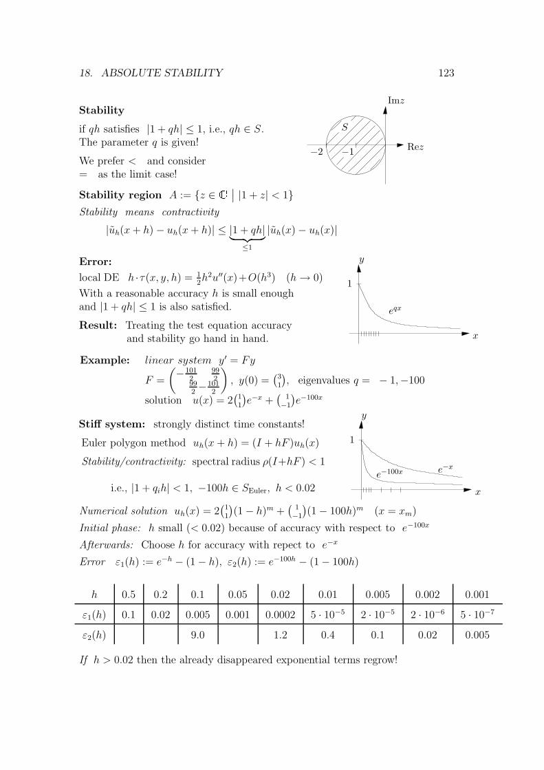
18. ABSOLUTE STABILITY 123
Stability
if qh satisfies |1 + qh| ≤ 1, i.e., qh ∈ S.The parameter q is given!
We prefer < and consider= as the limit case!
PSfrag replacements
−2 −1
S
Rez
Imz
Stability region A := {z ∈ �∣∣ |1 + z| < 1}
Stability means contractivity
|uh(x+ h)− uh(x+ h)| ≤ |1 + qh|︸ ︷︷ ︸≤1
|uh(x)− uh(x)|
Error:
local DE h ·τ(x, y, h) = 12h2u′′(x)+O(h3) (h→ 0)
With a reasonable accuracy h is small enoughand |1 + qh| ≤ 1 is also satisfied.
Result: Treating the test equation accuracyand stability go hand in hand.
PSfrag replacements1
y
eqx
x
Example: linear system y′ = Fy
F =
(−101
2992
992−101
2
), y(0) =
(31
), eigenvalues q = − 1,−100
solution u(x) = 2(
11
)e−x +
(1−1
)e−100x
Stiff system: strongly distinct time constants!
Euler polygon method uh(x + h) = (I + hF )uh(x)
Stability/contractivity: spectral radius ρ(I+hF ) < 1
i.e., |1 + qih| < 1, −100h ∈ SEuler, h < 0.02
PSfrag replacements1
y
e−100x e−x
x
Numerical solution uh(x) = 2(
11
)(1− h)m +
(1−1
)(1− 100h)m (x = xm)
Initial phase: h small (< 0.02) because of accuracy with respect to e−100x
Afterwards: Choose h for accuracy with repect to e−x
Error ε1(h) := e−h − (1− h), ε2(h) := e−100h − (1− 100h)
h 0.5 0.2 0.1 0.05 0.02 0.01 0.005 0.002 0.001
ε1(h) 0.1 0.02 0.005 0.001 0.0002 5 · 10−5 2 · 10−5 2 · 10−6 5 · 10−7
ε2(h) 9.0 1.2 0.4 0.1 0.02 0.005
If h > 0.02 then the already disappeared exponential terms regrow!
124
Wanted: Methods having a large stability region S
best possible with S ⊇ � − (left half plane) y absolute stability
Then choose h only with respect to accuracy!
Definition: A linear system y′ = Fy is called stiff, if it satisfies that alleigenvalues qj(F ) ∈ � − and
max |Reqi(F )|min |Reqi(F )| ≥ 50.
A nonlinear system y′ = f(x, y) is called stiff, if the linearized systemy′ = J(x)y is stiff for each admissible x.
One–step methods: Runge–Kutta (RK) methods (c, A, b)
U ′j = f(y + hΣajkU′k) (y = uh(x)) j = 1, . . . , s,
uh(x+ h) = y + hΣbjU′j
Application to the test equation
uh(x + h) = W (z)uh(x), z := qh
Because
U ′1...
U ′s
= eqy + qhA
U ′1...
U ′s
y (I − qhA)
U ′1...
U ′s
= eqy, e =
1...
1
uh(x+ h) = y + hbT
U ′1...
U ′s
=
(1 + qhbT (I − qhA)−1e
)y
Stability function W (z) := 1 + zbT (I − zA)−1e = det(I+zA)det(I−zA)
appr. exp(z)
Explicit RK method: W (z) = polynomial of degree ≤ s
s = p : W (z) = 1 + z + · · ·+ 1p!zp Taylor polynomial
Implicit RK method: W (z) = N(z)D(z)
, degree N ≤ s, degree D ≤ s
Implicit Euler method W (z) = 11−z (1, 1, 1)
Trapezoidal method W (z) =1+ 1
2z
1− 12z
0 0 0 1
2
1 12
12
12
Gaussian method (s = 1) W (z) =1+ 1
2z
1− 12z
(12, 1
2, 1)
Gaussian RK methods W (z) = N(z)D(z)
, degree N = degree D = s, order p = 2s
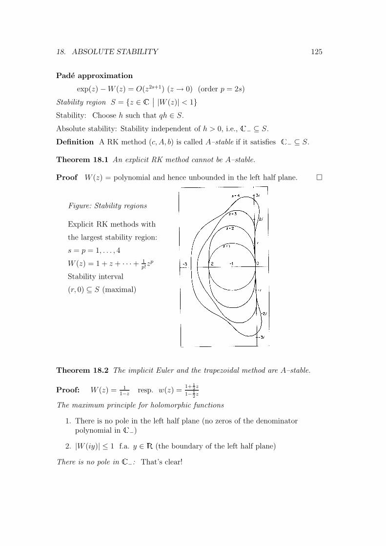
18. ABSOLUTE STABILITY 125
Pade approximation
exp(z) −W (z) = O(z2s+1) (z → 0) (order p = 2s)
Stability region S = {z ∈ �∣∣ |W (z)| < 1}
Stability: Choose h such that qh ∈ S.
Absolute stability: Stability independent of h > 0, i.e., � − ⊆ S.
Definition A RK method (c, A, b) is called A–stable if it satisfies � − ⊆ S.
Theorem 18.1 An explicit RK method cannot be A–stable.
Proof W (z) = polynomial and hence unbounded in the left half plane. �
Figure: Stability regions
Explicit RK methods with
the largest stability region:
s = p = 1, . . . , 4
W (z) = 1 + z + · · ·+ 1p!zp
Stability interval
(r, 0) ⊆ S (maximal)
Theorem 18.2 The implicit Euler and the trapezoidal method are A–stable.
Proof: W (z) = 11−z resp. w(z) =
1+ 12z
1− 12z
The maximum principle for holomorphic functions
1. There is no pole in the left half plane (no zeros of the denominatorpolynomial in � −)
2. |W (iy)| ≤ 1 f.a. y ∈ �(the boundary of the left half plane)
There is no pole in � −: That’s clear!
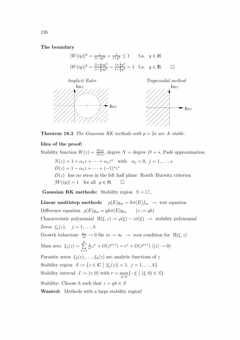
126
The boundary
|W (iy)|2 = 1|1−iy|2 = 1
1+y2 ≤ 1 f.a. y ∈ �
|W (iy)|2 =|1+ 1
2iy|2
|1− 12iy|2 =
1+ 14y2
1+ 14y2 = 1 f.a. y ∈ � �
Implicit Euler
PSfrag replacements
Imz
Rez
Trapezoidal method
PSfrag replacements
Imz
Rez
Theorem 18.3 The Gaussian RK methods with p = 2s are A–stable.
Idea of the proof:
Stability function W (z) = N(z)D(z)
, degree N = degree D = s, Pade approximation
N(z) = 1 + α1z + · · ·+ αszs with αj > 0, j = 1, . . . , s
D(z) = 1− α1z + · · ·+ (−1)szs
D(z) has no zeros in the left half plane: Routh–Hurwitz criterion
|W (iy)| = 1 for all y ∈ � �
Gaussian RK methods: Stability region S = � −
Linear multistep methods ρ(E)ym = hσ(E)fm → test equation
Difference equation ρ(E)ym = qhσ(E)ym (z := qh)
Characteristic polynomial Π(ξ, z) := ρ(ξ)− zσ(ξ) → stability polynomial
Zeros ξj(z), j = 1, . . . , k
Growth behaviour ymm→ 0 fur m→∞ → root condition for Π(ξ, z)
Main zero ξ1(z) =p∑
ν=1
1ν!zν +O(zp+1) = ez +O(zp+1) (|z| → 0)
Parasitic zeros ξ2(z), . . . , ξk(z) are analytic functions of z
Stability region S := {z ∈ �∣∣ |ξj(z)| < 1, j = 1, . . . , k}
Stability interval I := (r, 0) with r = maxξ<0{−ξ
∣∣ (ξ, 0) ∈ S}
Stability: Choose h such that z = qh ∈ SWanted: Methods with a large stability region!
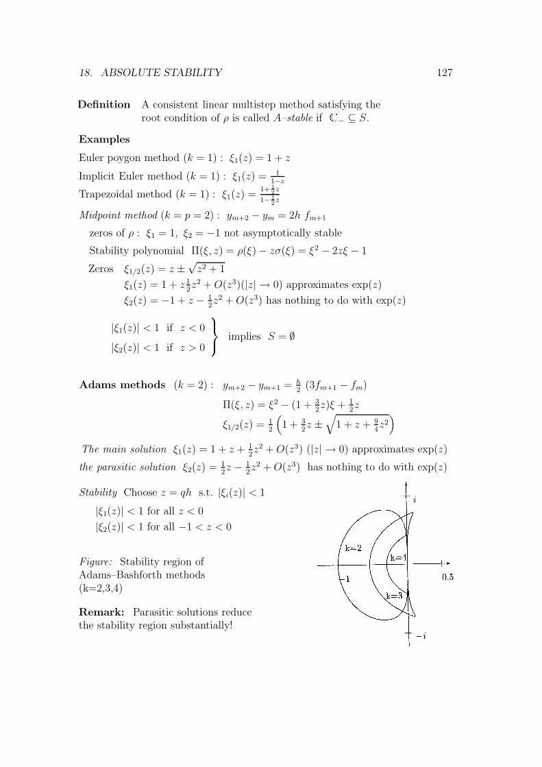
18. ABSOLUTE STABILITY 127
Definition A consistent linear multistep method satisfying theroot condition of ρ is called A–stable if � − ⊆ S.
Examples
Euler poygon method (k = 1) : ξ1(z) = 1 + z
Implicit Euler method (k = 1) : ξ1(z) = 11−z
Trapezoidal method (k = 1) : ξ1(z) =1+ 1
2z
1− 12z
Midpoint method (k = p = 2) : ym+2 − ym = 2h fm+1
zeros of ρ : ξ1 = 1, ξ2 = −1 not asymptotically stable
Stability polynomial Π(ξ, z) = ρ(ξ)− zσ(ξ) = ξ2 − 2zξ − 1
Zeros ξ1/2(z) = z ±√z2 + 1
ξ1(z) = 1 + z 12z2 +O(z3)(|z| → 0) approximates exp(z)
ξ2(z) = −1 + z − 12z2 +O(z3) has nothing to do with exp(z)
|ξ1(z)| < 1 if z < 0
|ξ2(z)| < 1 if z > 0
implies S = ∅
Adams methods (k = 2) : ym+2 − ym+1 = h2
(3fm+1 − fm)
Π(ξ, z) = ξ2 − (1 + 32z)ξ + 1
2z
ξ1/2(z) = 12
(1 + 3
2z ±
√1 + z + 9
4z2)
The main solution ξ1(z) = 1 + z + 12z2 +O(z3) (|z| → 0) approximates exp(z)
the parasitic solution ξ2(z) = 12z − 1
2z2 +O(z3) has nothing to do with exp(z)
Stability Choose z = qh s.t. |ξi(z)| < 1
|ξ1(z)| < 1 for all z < 0
|ξ2(z)| < 1 for all −1 < z < 0
Figure: Stability region ofAdams–Bashforth methods(k=2,3,4)
Remark: Parasitic solutions reducethe stability region substantially!
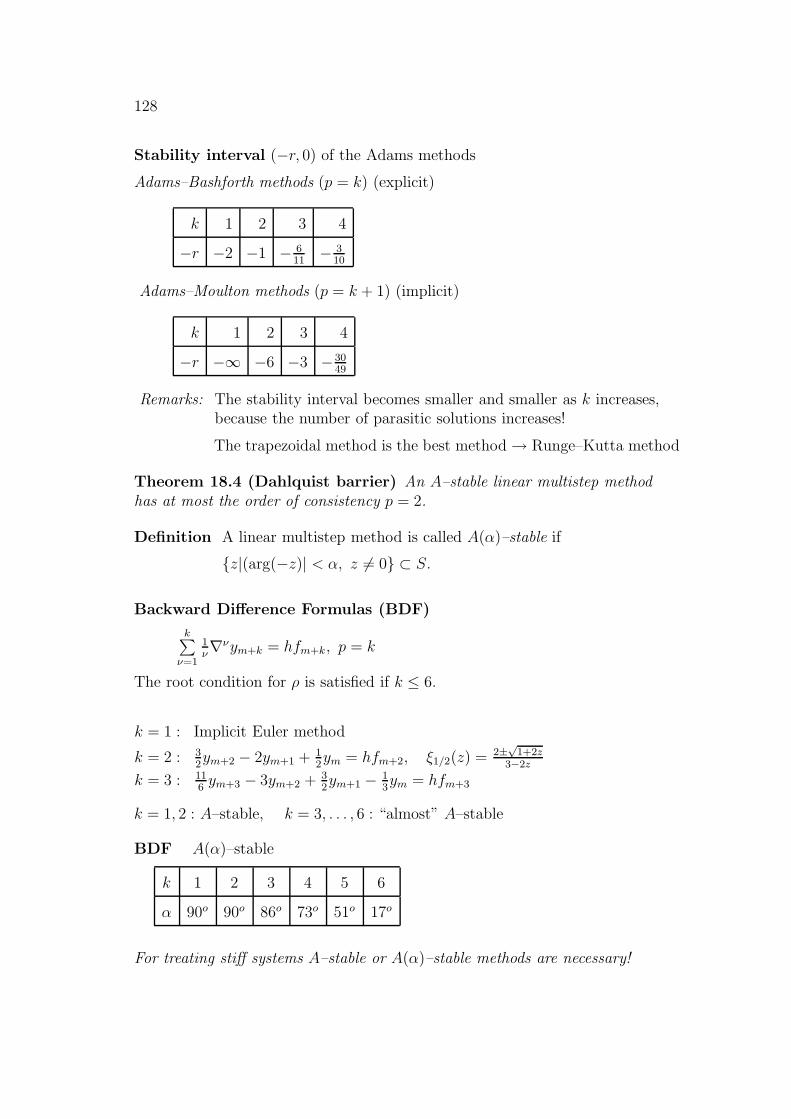
128
Stability interval (−r, 0) of the Adams methods
Adams–Bashforth methods (p = k) (explicit)
k 1 2 3 4
−r −2 −1 − 611− 3
10
Adams–Moulton methods (p = k + 1) (implicit)
k 1 2 3 4
−r −∞ −6 −3 − 3049
Remarks: The stability interval becomes smaller and smaller as k increases,because the number of parasitic solutions increases!
The trapezoidal method is the best method→ Runge–Kutta method
Theorem 18.4 (Dahlquist barrier) An A–stable linear multistep methodhas at most the order of consistency p = 2.
Definition A linear multistep method is called A(α)–stable if
{z|(arg(−z)| < α, z 6= 0} ⊂ S.
Backward Difference Formulas (BDF)
k∑ν=1
1ν∇νym+k = hfm+k, p = k
The root condition for ρ is satisfied if k ≤ 6.
k = 1 : Implicit Euler method
k = 2 : 32ym+2 − 2ym+1 + 1
2ym = hfm+2, ξ1/2(z) = 2±
√1+2z
3−2z
k = 3 : 116ym+3 − 3ym+2 + 3
2ym+1 − 1
3ym = hfm+3
k = 1, 2 : A–stable, k = 3, . . . , 6 : “almost” A–stable
BDF A(α)–stable
k 1 2 3 4 5 6
α 90o 90o 86o 73o 51o 17o
For treating stiff systems A–stable or A(α)–stable methods are necessary!
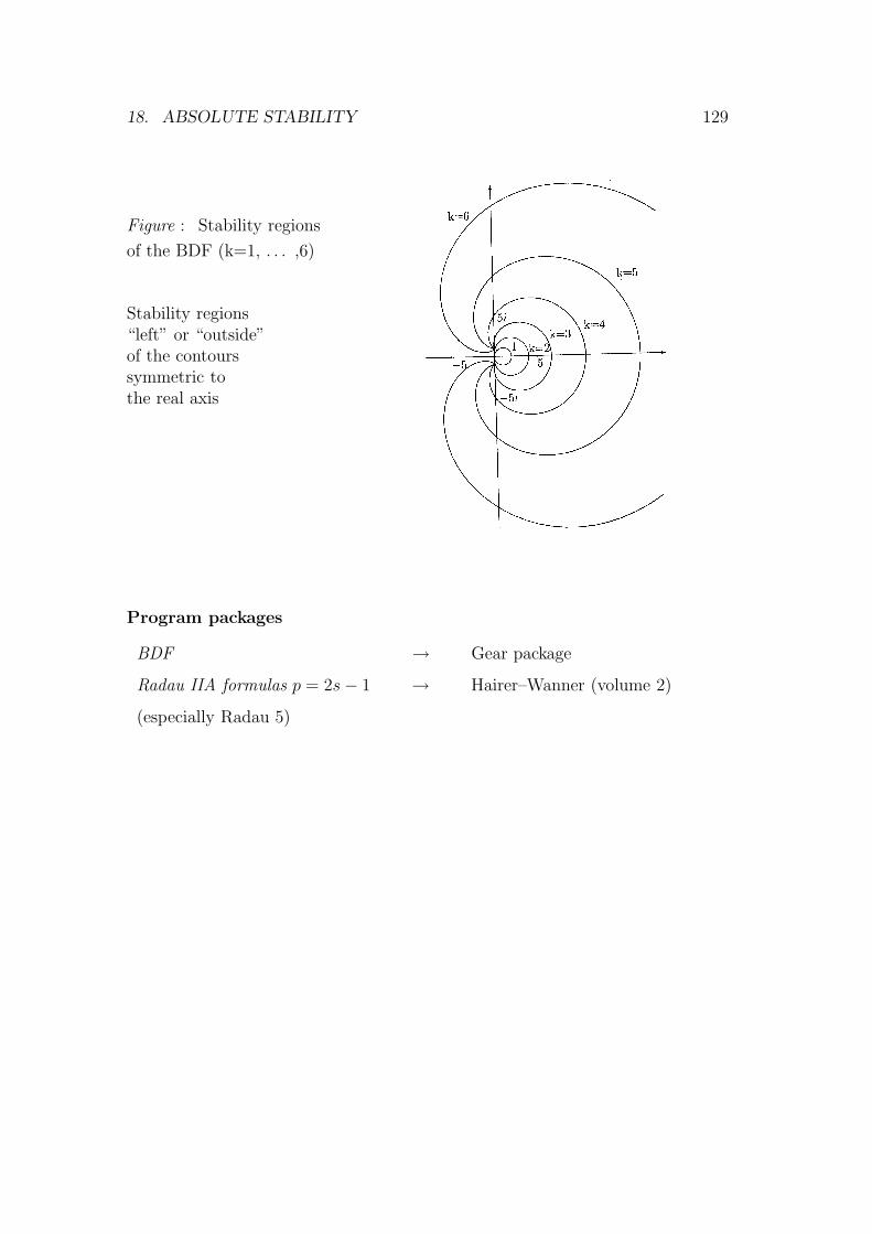
18. ABSOLUTE STABILITY 129
Figure : Stability regions
of the BDF (k=1, . . . ,6)
Stability regions“left” or “outside”of the contourssymmetric tothe real axis
Program packages
BDF → Gear package
Radau IIA formulas p = 2s− 1 → Hairer–Wanner (volume 2)
(especially Radau 5)


![[52] Sarvajit S. Sinha and Brian G. Schunck …iris.usc.edu/Outlines/papers/1995/liao-paper-95.pdf · [54] Stoer, J., and Bulirsch, R. 1980, inIntroduction to Numerical Analysis (New](https://img.pdfslide.net/doc/110x75/5b91ba6509d3f2f8508c3b98/52-sarvajit-s-sinha-and-brian-g-schunck-irisusceduoutlinespapers1995liao-paper-95pdf.jpg)


![Numerical Differentiation & Integration [0.125in]3.375in0 ...mamu/courses/231/Slides/CH04_4A.pdf · Numerical Differentiation & Integration Composite Numerical Integration I Numerical](https://img.pdfslide.net/doc/110x75/5b1fb63d7f8b9a112c8b4a5d/numerical-differentiation-integration-0125in3375in0-mamucourses231slidesch044apdf.jpg)