Embed Size (px)
Citation preview
Advanced Large-Eddy Simulation for lattice Boltzmann methods : the Approximate
Deconvolution Model
Orestis Malaspinas1, a) and Pierre Sagaut1, b)
Institut Jean Le Rond d’Alembert, UMR CNRS 7190, Universite Pierre et Marie
Curie - Paris 6
4, place Jussieu, case 162, F-75252 Paris cedex 5, France
(Dated: 25 October 2013)
The aim of this paper is to extend the Approximate Deconvolution Model for Large-
Eddy simulations to the lattice Boltzmann method. This approach allows to directly
act on the velocity distribution function and is based on the intrinsic nonlinearities of
the lattice Boltzmann methods. It is not a straightforward extrapolation of classical
eddy-viscosity models developed within the Navier–Stokes framework, which exhibits
a convective quadratic nonlinearity in the incompressible flow case. A simple imple-
mentation is presented, which relies on the implementation of an ad hoc linear filter
in any basic Lattice Boltzmann solver. The new model is validated on the turbulent,
time developing mixing layer, and a very satisfactory agreement is found with existing
direct numerical simulations results. The equivalent Navier-Stokes-type macroscopic
model is also discussed.
Keywords: Lattice Boltzmann Method, Turbulence modeling, Approximate decon-
volution model, Large Eddy Simulations, Time developing mixing layer
CONTENTS
I. Introduction 2
II. Approximate deconvolution model for the lattice Boltzmann method 4
A. The filtered Boltzmann equation 4
B. Approximate deconvolution method and lattice Boltzmann method 4
a)Electronic mail: [email protected])Electronic mail: [email protected]
C. Chapman–Enskog expansion of the ADM-BGK equation
D. Implementation of the ADM-BGK equation 8
E. Description of the filters used 8
III. The time dependent mixing layer 9
A. Numerical setup 9
B. Results 10
1
IV. Conclusion 12
Acknowledgements 14
References 14
I. INTRODUCTION
The simulation of turbulent flows is of pri-
mary importance in many everyday life ap-
plications. The wide increase in the range of
scales, involved in the motion of such flows,
with the Reynolds number forbids their Di-
rect Numerical Simulation (DNS) (where all
scales are simultaneously resolved) of many
applications of interest because of the lim-
ited capabilities of computers. In order to
study the behavior of this class of fluid flows
it is necessary to reduce the amount of de-
grees of freedom needed. One way of do-
ing this is by using Large Eddy Simulation
(LES) techniques (see Refs. 1–3) such as the
seminal Smagorinsky model4, where the main
idea is to resolve only the large scales of mo-
tion and to model the small ones. In this
way one is able to considerably reduce the
amount of degrees of freedom needed to simu-
late turbulent flows. Due to the nonlinearity
of the governing equations of motion, small
unresolved scales and large resolved scales are
coupled. Therefore, the removal of the small-
est scales of turbulence must be compensated
by a modification of the governing equations
for resolved scales, in order to account for
the effect of missing turbulent eddies. This is
done in practice by introducing a subgrid clo-
sure. The coupling terms directly stem from
the nonlinear term in the basic governing
equation since it can be defined as the com-
mutation error between nonlinear terms and
a linear scale separation operator. Therefore
a change in the nonlinear terms should in-
duce a change in the subgrid closure. Within
the Navier-Stokes framework, subgrid mod-
els have been improved in many ways dur-
ing the last decades, by accounting for new
physical phenomena (e.g. heat transfer 5 or
aeroacoustic noise generation6) or developing
multiscale/multidomain approaches 7 and 8,
but it is worth noting that the vast major-
ity of proposed subgrid closures relies on the
eddy viscosity paradigm.
In the lattice Boltzmann community the
huge majority of LES techniques is based
on “extrapolations” of eddy viscosity mod-
els for the Navier–Stokes equations, like the
Smagorinsky model (see Refs. 9–17 among
others). These models are based on a local
modification of the relaxation time in order
to modify the viscosity of the fluid. A first
remark is that the direct plugging of Navier-
Stokes-based eddy viscosity via a change of
the relaxation time in BGK-type methods
does not guarantee that the features of the
non-linear collision term, which does not ex-
2
hibit the same nonlinear character as the con-
vection term in incompressible Navier-Stokes
equations, are taken into account in a fully
satisfactory way. A second remark is that
Lattice Boltzmann methods can capture dif-
ferent kinds of physics, ranging from incom-
pressible to fully compressible flows, depend-
ing on the truncation order of the Hermite
polynomial based series expansion of the ex-
ponential nonlinear collision term (and there-
fore on the order of the nonlinear collision
term). As a consequence, a general sub-
grid closure procedure which automatically
adapts itself to nonlinear terms should be
sought for.
To this end, we propose here to reuse
the idea of the Approximate Deconvolu-
tion Model (ADM) of Stolz, Adams and
Kleiser18–20 where the macroscopic fields
(density, velocity, ...) are approximately re-
covered by applying an approximate inverse
filter operator on the filtered Navier–Stokes
equations. This approach, which does not as-
sume any particular feature of the nonlinear
terms and the underlying interscale physics,
has successfully been applied to both incom-
pressible and compressible flows, including
flows with shock waves21.
In our case, instead of acting on the
macroscopic fields, we apply the Approxi-
mate Deconvolution operator directly on the
filtered distribution function, which is the
basis of the Boltzmann equation, as pro-
posed by Sagaut22. Thus, instead of rely-
ing only on macroscopic modeling of turbu-
lence, one is able to act directly on a more
microscopic level, which provides an alter-
nate methodology. Another point is that
each filtered lattice Boltzmann model for
large-eddy simulations can be associated with
a corresponding macroscopic Navier-Stokes-
like equations. Since filtering the Lattice
Boltzmann governing equation is uniquely
defined, it can also represent an interesting
way to derive governing equations for Navier-
Stokes based large-eddy simulation for com-
pressible flows, since direct filtering of com-
pressible Navier-Stokes equations is known
to lead to an infinity of possible set of
equations3.
The organization of this paper is as fol-
lows. In Sec. II the ADM is presented and is
applied in the LBM framework. The model is
then validated on the time dependent mixing
layer in Sec. III which is a classical turbu-
lence benchmark. And finally the paper is
concluded in Sec. IV.
3
II. APPROXIMATE
DECONVOLUTION MODEL FOR
THE LATTICE BOLTZMANN
METHOD
In this section, following the paper by
Sagaut22, the approximate deconvolution
method for LBM-LES will be presented.
A. The filtered Boltzmann equation
The continuous Boltzmann equation in
absence of an external force with a generic
collision operator Ω(f) reads
df
dt≡ (∂t + ξ ·∇x) f = Ω(f), (1)
where f is the density probability distribu-
tion of finding a particle with velocity ξ at
position x at time t. The macroscopic ob-
servables are as usual given in terms of mo-
ments of f
ρ =
∫
dξ f, ρu =
∫
dξ ξf. (2)
With G a convolution filter kernel, and denot-
ing the filtered counterpart of any quantity,
a, as a ≡ G ∗ a, one can write the filtered
Boltzmann equation as
df
dt= Ω(f) ⇔ df
dt− Ω(f) = R, (3)
where R ≡ Ω(f) − Ω(f) corresponds to the
subgrid term that has to be modeled and rep-
resents the error of the commutator of the
collision and the filtering operators.
B. Approximate deconvolution
method and lattice Boltzmann method
We now use the idea developed by Stolz
and Adams18–20 of trying to reconstruct the
unfiltered-filtered fields in an approximate
manner. To this aim we define an easy to
compute inverse filter approximation Q
Q ∗ G = I +O(hl), (4)
where I is the identity, h a measure of the
grid resolution and l > 0 the order of the
reconstruction. Defining f ∗ ≡ Q ∗ f , one
can rewrite the r.h.s. of Eq. (3) following the
approach by Mathew et al.23,
R = R1 +R2 = Ω(f ∗)− Ω(f)+ Ω(f)− Ω (f ∗), where
(5)
R1 ≡ Ω (f ∗)− Ω(f), R2 ≡ G ∗ [Ω(f)− Ω (f ∗)] .
(6)
We will now focus our attention on R2, the
part of R that needs to be modeled. Under
the assumption that |f−f ∗| ≪ 1, one can do
a Taylor expansion of Ω(f ∗) around f up to
order one
R2∼= −G∗
[
∂f∗Ω∣∣f(f ∗ − f)
]
= G∗[
∂f∗Ω∣∣f(Q ∗ G − I) ∗ f
]
.
(7)
Inspired by the work of Mathew et al.23 one
replaces f by f ∗ to close this equation
R2∼= −G ∗
[
(Q ∗ G − I) ∗ f ∗∂f∗Ω∣∣f=f∗
]
.
(8)
4
The assumption |f − f ∗| ≪ 1 is actually true
only if the filter width is in the dissipation
range which is true only if the simulation is
completely resolved. In our case we rather
have that the large scales of f are close to
those of f ∗ and since we are aiming for a
model for the resolved scales the Taylor ex-
pansion remains valid.
With this approximation one can rewrite
Eq. (3) as
G∗(df ∗
dt− Ω (f ∗)
)
= G∗[
(I −Q ∗ G) ∗ f ∗∂f∗Ω∣∣f=f∗
]
.
(9)
Specifying now the collision operator as
the standard BGK (Bhatnagar, Gross and
Krook24), and following the standard velocity
discretization procedure of the Boltzmann-
BGK equation proposed in Shan et al.25 (see
also Ref. 26) Eq. (9) reads
G ∗(df ∗
dt+ ω
(
f ∗
i − f(0)i (f ∗)
))
=
− ωG ∗
∑
j
∂f∗
j
(
f ∗
i − f(0)i (f ∗)
)∣∣∣∣∣f=f∗
(I −Q ∗ G) ∗ f ∗
j
︸ ︷︷ ︸
≡Ri,bgk
,
(10)
where ω is the relaxation frequency, f ∗
i ≡f ∗(x, ξi, t) is the velocity-discretized distri-
bution function (with ξi the q abscissae of the
Gauss–Hermite quadrature), the f(0)i (f ∗) are
the Hermite expanded Maxwell distribution
up to an arbitrary order (corresponding to
the Gauss–Hermite quadrature order) evalu-
ated with the moments of f ∗
kq−1k=0.
When truncating the Hermite expansion
of the equilibrium distribution up to or-
der two, the macroscopic limit of the BGK
equation gives asymptotically the weakly
compressible Navier–Stokes equations (see
Ref. 27). The equilibrium distribution is then
found to be
f(0)i (f) = wiρ
(
1 +ξi · uc2s
+1
2c4sH(2)
i : uu
)
,
(11)
where ρ =∑
i fi, j ≡ ρu =∑
i ξifi, “:”
is the full index contraction and H(2)i ≡
ξiξi − c2sI (I being the identity, wi and cs
the weights and the speed of sound of the
lattice). Defining ∆a ≡ (I − Q ∗ G) ∗ a (a
being an arbitrary quantity), and specifying
5
f(0)i allows us to evaluateRi,bgk (see Eq. (10))
Ri,bgk =∑
j
∂f∗
j
[
f ∗
i − wi
(∑
k
f ∗
k +ξi
c2s·∑
k
ξkf∗
k
+1
2c4s
(∑
m
f ∗
m
)−1
H(2)i :
∑
k
ξkf∗
k
∑
l
ξlf∗
l
)]
f=f∗
∆f ∗
j ,
(12)
=∑
j
[
δij − wi
(∑
k
δjk +ξi · ξjc2s
+1
2c4sH(2)
i :
(
−(∑
m
fm
)−2∑
n
δnj∑
k
ξkfk∑
l
ξlfl
+
(∑
m
fm
)−1
ξj∑
l
ξlfl +
(∑
m
fm
)−1∑
l
ξlflξj
))]
f=f∗
∆f ∗
j ,
(13)
= ∆f ∗
i − wi
(
∆ρ∗ +ξi · (∆j∗)
c2s
+1
2c4sH(2)
i :
(
−∆ρ∗
ρ∗2j∗j∗ +
1
ρ∗∆j∗j∗ +
1
ρ∗j∗∆j∗
))
.
(14)
Therefore Eq. (10) becomes
G∗(df ∗
dt+ ω
(
f ∗
i − f(0)i (f ∗)
))
= −ωG∗Ri,bgk.
(15)
This last equation is the complete ADM-
BGK equation. Following the conclusions
of Mathew et al.23, the R2 term can be ne-
glected without noticeable effects on the re-
sults of the simulations to obtain a further
simplified model
G ∗(df ∗
dt− Ω (f ∗)
)
= 0. (16)
The advantage of this approximation is that
the implementation is completely straight-
forward since, apart from the filtering step,
the LBM time marching scheme remains ex-
actly the same as for DNS computations.
We therefore have the normal collide-and-
stream process followed by the filtering op-
eration (the implementation details are dis-
cussed later).
C. Chapman–Enskog expansion of
the ADM-BGK equation
In this section the Chapman–Enskog (CE)
expansion of the ADM-BGK equation is dis-
cussed. The CE expansion is based on the
assumption that the non-filtered distribution
function is given by its local equilibrium value
to which a small perturbation (proportional
to the Knudsen number) is added
fi = f(0)i + f
(1)i , f
(1)i ≪ f (0). (17)
Here our formulation of the BGK equation is
based on the approximate deconvolution of
the distribution function. We therefore want
to write their CE equivalent for f ∗
i
f ∗
i = Q ∗ G ∗ fi =(
f(0)i
)∗
+(
f(1)i
)∗
. (18)
The difference between the approximate de-
convolution and the “bare” distribution func-
tions is of order O(hl) (see Eq. (4)). Since,
the LBM is known to be second order ac-
curate in space, O(h2) (see Refs. 26–28), by
choosing carefully the filter and the deconvo-
lution one can argue that the difference be-
tween f(0)i (f ∗) and (f
(0)i )∗ (and thus between
6
f(1)i (f ∗) and (f
(1)i )∗) can be made smaller
than the order of the method
f ∗
i∼= f
(0)i (f ∗) + f
(1)i (f ∗). (19)
Therefore the CE expansion of the ADM–
BGK equation is very similar to what can
be found is the literature (see Refs. 27 and
29 for more details).
Taking the zeroth and first order moment
of Eq. (15), one gets
∂tρ∗ +∇ · j∗ = −ω
∑
i
Ri,bgk, (20)
∂tj∗ +∇ ·
(j∗j∗
ρ∗
)
+∇ · P ∗ = −ω∑
i
ξiRi,bgk,
(21)
where P ∗ =∑
i(ξi − j∗/ρ∗)(ξi − j∗/ρ∗)f ∗
i .
Replacing f ∗
i by their CE expansion and
keeping only the lower order terms in
Eq. (15), one gets (for simplicity we apply
G−1 on both sides of the equation and the
dependence on f ∗ is understood in f(0)i and
f(1)i )
df(0)i
dt+ ωf
(1)i = −ω
[
∆f(0)i − wi
(
∆ρ∗ +ξi · (∆j∗)
c2s
+1
2c4sH(2)
i :
(
−∆ρ∗
ρ∗2j∗j∗ +
1
ρ∗∆j∗j∗ +
1
ρ∗j∗∆j∗
))]
= −wiω
2c4sH(2)
i :
[
∆
(j∗j∗
ρ∗
)
+∆ρ∗
ρ∗2j∗j∗ − 1
ρ∗∆j∗j∗ − 1
ρ∗j∗∆j∗
]
.
(22)
where in the second line we used that
f(0)i (f ∗) = wi
(
ρ∗ +ξi · j∗c2s
+1
2c4sH(2)
i :j∗j∗
ρ∗
)
.
(23)
Taking the zeroth and first order moments
of Eq. (22) one finds the equivalent of Euler
equations
∂tρ∗ +∇ · j∗ = 0, (24)
∂tj∗ +∇ ·
(j∗j∗
ρ∗
)
= −∇p∗, (25)
where p∗ = c2sρ∗. To go to the Navier–Stokes
level, the evaluation of the second order mo-
ment of Eq. (22) is needed. After some te-
dious algebra one finds
∑
i
H(2)i f
(1)i = −c2s
ωρ∗
[
∇
(j∗
ρ∗
)
+
(
∇
(j∗
ρ∗
))T]
+∆
(j∗j∗
ρ∗
)
+∆ρ∗
ρ∗2j∗j∗ − 1
ρ∗∆j∗j∗ − 1
ρ∗j
(26)
where the superscript “T” stands for the
transpose operation. Finally, setting P ∗ =∑
i(ξi − j∗/ρ∗)(ξi − j∗/ρ∗)(f(0)i + f
(1)i ) in
Eq. (21), the Navier–Stokes limit of the
ADM-BGK equation reads
∂tj∗ +∇ ·
(j∗j∗
ρ∗
)
=−∇p∗ + 2µ∇ · S∗
−∇ ·(
∆
(j∗j∗
ρ∗
)
+∆ρ∗
ρ∗2j∗j∗ − 1
ρ∗∆
(27)
where µ = c2sρ∗/ω and S∗ = (∇(j∗/ρ∗) +
∇(j∗/ρ∗)T)/2. This equation corresponds to
Eq. (A2) of the work by Mathew et al.23.
When using the simplified collision of
Eq. (16) the momentum conservation equa-
tion is reduced to
∂tj∗+∇·
(j∗j∗
ρ∗
)
= −∇p∗+2µ∇·S∗. (28)
7
In what follows we will only consider the sim-
plified model.
D. Implementation of the
ADM-BGK equation
After discretization of time and space us-
ing the standard trapezoidal rule and change
of variables (see Ref. 30), the algorithm for
the simulation of weakly compressible fluids,
is therefore given by
1. Standard collide and stream process
(δx = δt = 1)
f ∗
iout(x+ξi, t+1) = f ∗
iin(x, t)−ω
(
f ∗
iin(x, t)− f
(0)i
∗
(x, t))
,
(29)
where ω is the relaxation frequency
f(0)i
∗
= wi
(
ρ∗ +ξi · j∗c2s
+H(2)
i
2c4s:j∗j∗
ρ∗
)
,
(30)
and where ρ∗ =∑
i f∗
iin, j∗ =
∑
i ξif∗
iin.
2. Application of the explicit filtering op-
eration
f ∗
iin = Q ∗ G ∗ f ∗
iout, ∀i. (31)
The ADM operator Q ∗ G is described
in more details in the next subsection.
In the collision–streaming steps we used the
order two truncation of the equilibrium dis-
tribution function in Hermite polynomials in
order to simulate weakly compressible fluids.
The reader should be aware that the ADM is
independent of this choice and therefore can
be extended straightforwardly to compress-
ible and thermal flows by changing the trun-
cation order of the equilibrium as well as the
lattice definition (see Ref. 25).
E. Description of the filters used
The filtering operation is done with the
filters proposed in Ricot et al.31. They are
given by
Q∗G∗f ∗
i = f ∗
i (x, t)−σD∑
j=1
N∑
n=−N
dnf∗
i (x+ nej , t) ,
(32)
where the ei are theD-dimensional Cartesian
basis vectors, 2N +1 is the number of points
of the filter stencil, and σ ∈ [0, 1] is the filter
strength. The dn = d−n are obtained by can-
celing the Taylor expansion of the last term
of r.h.s. of this last equation and canceling
order by order up to the desired expansion
order NN∑
n=−N
nkdn = 0, 0 ≤ k ≤ 2N + 1. (33)
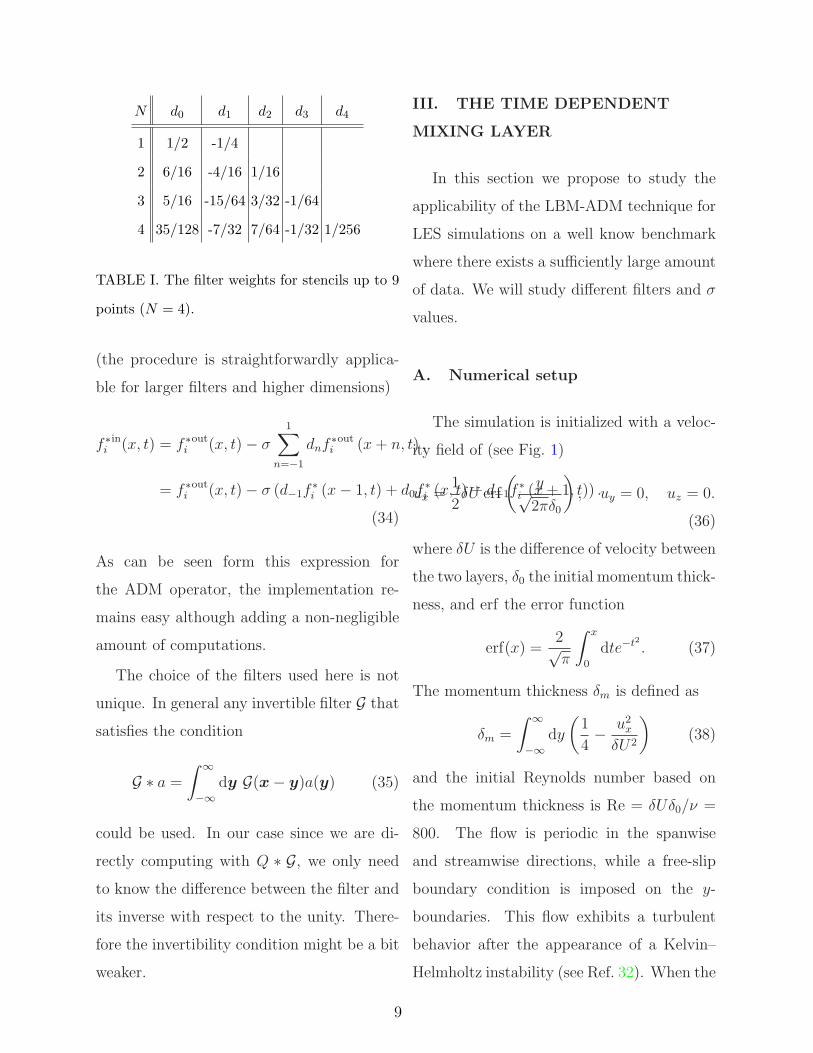
The values for the dn coefficients are given
in Table I for different N values. The ADM
operation is therefore non-local since it needs
to access N neighbors in each D direction for
all the q discrete velocities ξi.
Finally, for the sake of clarity, let us write
down the 3-points filter ADM operator in 1D
8
N d0 d1 d2 d3 d4
1 1/2 -1/4
2 6/16 -4/16 1/16
3 5/16 -15/64 3/32 -1/64
4 35/128 -7/32 7/64 -1/32 1/256
TABLE I. The filter weights for stencils up to 9
points (N = 4).
(the procedure is straightforwardly applica-
ble for larger filters and higher dimensions)
f ∗
iin(x, t) = f ∗
iout(x, t)− σ
1∑
n=−1
dnf∗
iout (x+ n, t) ,
= f ∗
iout(x, t)− σ (d−1f
∗
i (x− 1, t) + d0f∗
i (x, t) + d+1f∗
i (x+ 1, t)) .
(34)
As can be seen form this expression for
the ADM operator, the implementation re-
mains easy although adding a non-negligible
amount of computations.
The choice of the filters used here is not
unique. In general any invertible filter G that
satisfies the condition
G ∗ a =
∫∞
−∞
dy G(x− y)a(y) (35)
could be used. In our case since we are di-
rectly computing with Q ∗ G, we only need
to know the difference between the filter and
its inverse with respect to the unity. There-
fore the invertibility condition might be a bit
weaker.
III. THE TIME DEPENDENT
MIXING LAYER
In this section we propose to study the
applicability of the LBM-ADM technique for
LES simulations on a well know benchmark
where there exists a sufficiently large amount
of data. We will study different filters and σ
values.
A. Numerical setup
The simulation is initialized with a veloc-
ity field of (see Fig. 1)
ux =1
2δU erf
(y√2πδ0
)
, uy = 0, uz = 0.
(36)
where δU is the difference of velocity between
the two layers, δ0 the initial momentum thick-
ness, and erf the error function
erf(x) =2√π
∫ x
0
dte−t2 . (37)
The momentum thickness δm is defined as
δm =
∫∞
−∞
dy
(1
4− u2
x
δU2
)
(38)
and the initial Reynolds number based on
the momentum thickness is Re = δUδ0/ν =
800. The flow is periodic in the spanwise
and streamwise directions, while a free-slip
boundary condition is imposed on the y-
boundaries. This flow exhibits a turbulent
behavior after the appearance of a Kelvin–
Helmholtz instability (see Ref. 32). When the
9
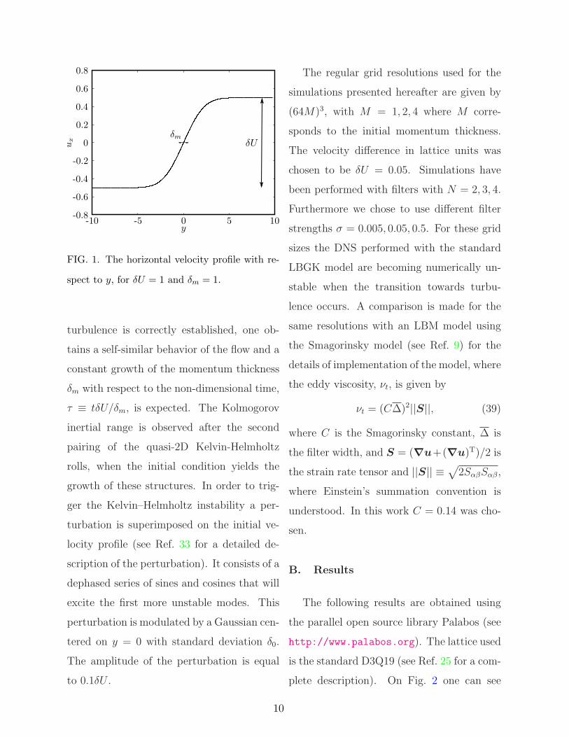
FIG. 1. The horizontal velocity profile with re-
spect to y, for δU = 1 and δm = 1.
turbulence is correctly established, one ob-
tains a self-similar behavior of the flow and a
constant growth of the momentum thickness
δm with respect to the non-dimensional time,
τ ≡ tδU/δm, is expected. The Kolmogorov
inertial range is observed after the second
pairing of the quasi-2D Kelvin-Helmholtz
rolls, when the initial condition yields the
growth of these structures. In order to trig-
ger the Kelvin–Helmholtz instability a per-
turbation is superimposed on the initial ve-
locity profile (see Ref. 33 for a detailed de-
scription of the perturbation). It consists of a
dephased series of sines and cosines that will
excite the first more unstable modes. This
perturbation is modulated by a Gaussian cen-
tered on y = 0 with standard deviation δ0.
The amplitude of the perturbation is equal
to 0.1δU .
The regular grid resolutions used for the
simulations presented hereafter are given by
(64M)3, with M = 1, 2, 4 where M corre-
sponds to the initial momentum thickness.
The velocity difference in lattice units was
chosen to be δU = 0.05. Simulations have
been performed with filters with N = 2, 3, 4.
Furthermore we chose to use different filter
strengths σ = 0.005, 0.05, 0.5. For these grid
sizes the DNS performed with the standard
LBGK model are becoming numerically un-
stable when the transition towards turbu-
lence occurs. A comparison is made for the
same resolutions with an LBM model using
the Smagorinsky model (see Ref. 9) for the
details of implementation of the model, where
the eddy viscosity, νt, is given by
νt = (C∆)2||S||, (39)
where C is the Smagorinsky constant, ∆ is
the filter width, and S = (∇u+(∇u)T)/2 is
the strain rate tensor and ||S|| ≡√2SαβSαβ,
where Einstein’s summation convention is
understood. In this work C = 0.14 was cho-
sen.
B. Results
The following results are obtained using
the parallel open source library Palabos (see
http://www.palabos.org). The lattice used
is the standard D3Q19 (see Ref. 25 for a com-
plete description). On Fig. 2 one can see
10

snapshots of the simulation at times, t =
0, 125, 250, 375, 500. There, the x-component
of the velocity and the iso-surfaces of the Q-
criterion (different at each time) are depicted.
The initial perturbation at time t = 0 slowly
develops into a turbulent flow after t ∼= 250,
and one can see the well known worm-like
structures forming. The filters width as well
FIG. 2. Iso-surfaces of the Q-criterion and ux
at times t = 0, 125, 250, 375, 500 (from left to
right and top to bottom). In black the velocity
is negative while it is positive in light gray.
as their strength must be carefully chosen,
in order to allow the instability to develop
properly. To our knowledge there exist no
way to determine them a priori but must be
tuned depending on the physical problem un-
der consideration. For instance, in our case,
the N = 1 (three points) filter never exhibits
a turbulent behavior. While in the case of
the N = 2 the development of turbulence
can be observed but not for any value of
σ. The σ = 0.5, 0.05, 0.005 strengths are de-
picted in Fig. 3, where one can see that for
σ = 0.5, 0.05 the increase rate of the momen-
tum thickness seems way too underestimated,
indicating that the Kelvin–Helmholtz insta-
bility is never initiated and the subsequent
turbulent behavior never occurs. On the con-
trary, for σ = 0.005, the self-similar period is
present.
FIG. 3. The momentum thickness with respect
to the normalized time τ = tδU/δm for N = 2
and σ = 0.5, 0.05, 0.005.
In order to validate that the simulation is
converging with the grid resolution, we per-
formed a series of measurements for M =
1, 2, 4 (resolutions of 643, 1283, 2563) for all
filter widths for σ = 0.005. As can be seen
from Fig. 4 the increase rate of the momen-
tum thickness is very similar for all simula-
tions. The main difference is the moment
where the instability is initiated. From now
11

FIG. 4. The momentum thickness with respect
with the non-dimensional time τ = tδU/δm for
N = 2, 3, 4 and σ = 0.005 for M = 1, 2, 4 as well
as for the Smagorinsky model for M = 1.
on, only the case of M = 1 is considered.
In the work by Rogers and Moser32, the
growth rate r = dδm/dτ was found to be
r = 0.014 in agreement with the experimen-
tal data of Dimotakis34 (0.014-0.021). In the
present study, the value of r varies slightly
depending on the filters width as shown in
Table II. While the analytical models pro-
posed here are completely generic a specific
filter has been chosen for implementation
purposes.
The self similar behavior is also confirmed
by the fact that instantaneous averaged ve-
locity profiles 〈ux(y)〉 and the r.m.s. velocity
〈u′
x(y)2〉, where y ≡ y/δm(t), are superim-
posed for five times (see Figs 5 and 6).
On Fig. 7 the one dimensional energy
N = 2 N = 3 N = 4 Smagorinsky
r 0.012 0.013 0.013 0.013
TABLE II. Value of the momentum thickness
growth rate r for the different filters width and
for the Smagorinsky model.
spectrum with respect to the kx is depicted.
It can be seen that the expected k−5/3x energy
slope is relatively well recovered. The spec-
trum of the 5 and 7-points filter seems to be
a bit “off” the −5/3 slope while the 9-points
filter gives better result, which seem even a
bit closer to the k−5/3x than those obtained
using the the Smagorinsky model.
IV. CONCLUSION
In the present paper we applied the ap-
proximate deconvolution model to the lattice
Boltzmann method. We proposed two levels
of approximation for the closure of the decon-
voluted equation. We showed that the sim-
plified ADM-LBM model represents correctly
the dynamics of turbulent flows by simulating
the turbulent mixing layer. The self-similar
behavior as well as the energy spectrum is
recovered correctly with a limited amount of
grid points.
The ADM–LBM has the advantage of not
relying on “extrapolations” of Navier–Stokes
turbulence models applied to the LBM, since
12
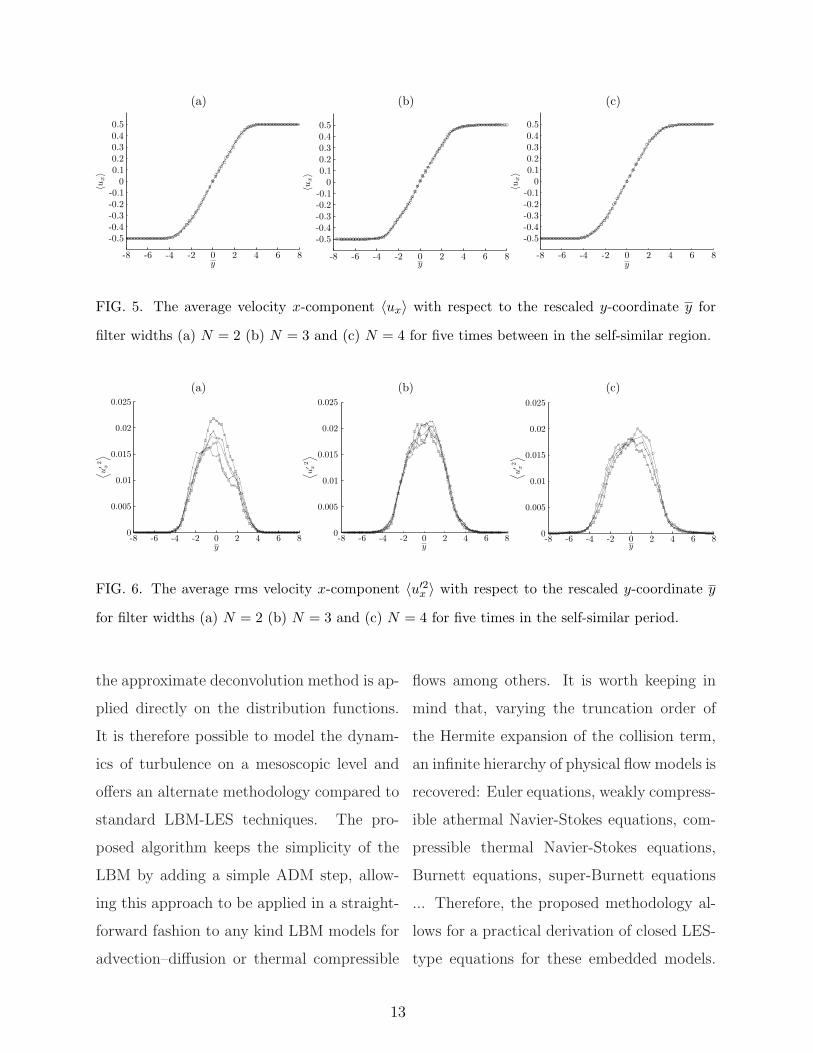
FIG. 5. The average velocity x-component 〈ux〉 with respect to the rescaled y-coordinate y for
filter widths (a) N = 2 (b) N = 3 and (c) N = 4 for five times between in the self-similar region.
FIG. 6. The average rms velocity x-component 〈u′2x 〉 with respect to the rescaled y-coordinate y
for filter widths (a) N = 2 (b) N = 3 and (c) N = 4 for five times in the self-similar period.
the approximate deconvolution method is ap-
plied directly on the distribution functions.
It is therefore possible to model the dynam-
ics of turbulence on a mesoscopic level and
offers an alternate methodology compared to
standard LBM-LES techniques. The pro-
posed algorithm keeps the simplicity of the
LBM by adding a simple ADM step, allow-
ing this approach to be applied in a straight-
forward fashion to any kind LBM models for
advection–diffusion or thermal compressible
flows among others. It is worth keeping in
mind that, varying the truncation order of
the Hermite expansion of the collision term,
an infinite hierarchy of physical flow models is
recovered: Euler equations, weakly compress-
ible athermal Navier-Stokes equations, com-
pressible thermal Navier-Stokes equations,
Burnett equations, super-Burnett equations
... Therefore, the proposed methodology al-
lows for a practical derivation of closed LES-
type equations for these embedded models.
13

FIG. 7. The instantaneous energy spectrum
E(k) with respect to kx and the expected k−5/3x
slope.
Extending LES to higher-order models, such
as Burnett equations, the relative influence of
the R2 term and the required filter strength
need to be re-investigated.
In principle, the method could also be ex-
tended to multiple relaxation time models
and not only be restricted to the standard
BGK. In the same way, the proposed Approx-
imate Deconvolution approach makes it easy
to handle non-linear source terms.
An actual implementation of Eq. (15)
and a comparison with the simplified model
implemented in the present work is left
for future work. Furthermore, as sug-
gested in previous papers dealing with the
Navier–Stokes framework the filters used
seem to have an influence on the resolved
scales, especially in wall-bounded flows in
which turbulence-generating instabilities are
dissipation-dependent. Such effects might be
interesting to test on the LBM–ADM.
ACKNOWLEDGEMENTS
O. Malaspinas would like to thankfully ac-
knowledge the support of the Swiss National
Science Foundation SNF (Award PBELP2-
133356) and the Department of Theoretical
Physics of the University of Geneva for allow-
ing the use of the Andromeda cluster. Pierre
Sagaut acknowledges the support of FUI via
the LaBS project.
REFERENCES
1P. Sagaut, Large Eddy Simulation for
Incompressible Flows: An Introduction
(Springer, Berlin, 2001).
2E. Garnier, N.A. Adams, and P. Sagaut,
Large Eddy Simulation for Compressible
Flows (Springer, Berlin, 2009).
3P. Sagaut, S. Deck, and M. Terracol, Mul-
tiscale and Multiresolution Approaches in
turbulence (Imperial College Press, Lon-
don, 2009).
4J. Smagorinsky, “General circulation exper-
iments with the primitive equations: I. the
basic equations,” Mon. Weather Rev. 91,
99–164 (1963).
14
5O. Labbe,E. Montreuil,P. Sagaut, “Large-
eddy simulation of heat transfer over a
backward facing step,” Int. J. Numer. Heat
Transfer - Part A. 42, 73–90 (2002).
6C. Seror,P. Sagaut,C. Bailly,D. Juve, “On
the radiated noise computed by Large-
eddy simulation,” Phys. Fluids 13, 476–487
(2001).
7P. Quemere,P. Sagaut,V. Couaillier, “A
new multidomain/multiresolution method
for large-eddy simulation,” Int. J. Numer.
Methods Fluids 36, 391–416 (2001).
8P. Quemere,P. Sagaut, “Zonal multidomain
RANS/LES simulation of turbulent flows,”
Int. J. Numer. Methods Fluids 40, 903–925
(2002).
9S. Hou, J. Sterling, S. Chen, and G. D.
Doolen, “A lattice Boltzmann subgrid
model for high Reynolds number flows,”
Fields Inst. Comm. 6, 151–66 (1996).
10Jack G. M. Eggels, “Direct and large-
eddy simulation of turbulent fluid flow
using the lattice-Boltzmann scheme,”
Int. J. Heat Fluid Flow 17, 307 – 323
(1996).
11O. Filippova, S. Succi, F. Mazzocco, C. Ar-
righetti, G. Bella, and D. Hanel, “Multi-
scale lattice Boltzmann schemes with tur-
bulence modeling,” J. Comp. Phys. 170,
812 – 829 (2001).
12M. Krafczyk, J. Tolke, and L.-S. Luo,
“Large-eddy simulations with a multiple-
relaxation-time LBE model,” Int. J. Mod.
Phys. B 17, 33–39 (2003).
13J. Kerimo and S. Girimaji, “Boltzmann-
BGK approach to simulating weakly com-
pressible 3D turbulence: comparison be-
tween lattice Boltzmann and gas kinetic
methods,” J. Turbul. 8 (2007).
14Y.-H. Dong, P. Sagaut, and S. Marie, “Iner-
tial consistent subgrid model for large-eddy
simulation based on the lattice Boltzmann
method,” Phys. Fluids 20, 035104 (2008)
15K. N. Premnath, M. J. Pattison, and
S. Banerjee, “Dynamic subgrid scale mod-
eling of turbulent flows using lattice-
Boltzmann method,” Physica A 388, 2640
– 2658 (2009).
16S. Chen, “A large-eddy-based lattice Boltz-
mann model for turbulent flow simula-
tion,” Appl. Math. Comput. 215, 591 – 598
(2009).
17M. Weickert, G. Teike, O. Schmidt, and
M. Sommerfeld, “Investigation of the
LES WALE turbulence model within
the lattice Boltzmann framework,”
Comput. Math. Appl. 59, 2200 – 2214
(2010).
18S. Stolz and N. A. Adams, “An approx-
imate deconvolution procedure for large-
eddy simulation,” Phys. Fluids 11, 1699–
1701 (1999).
19S. Stolz, N. A. Adams, and L. Kleiser, “An
approximate deconvolution model for large-
15
eddy simulation with application to incom-
pressible wall-bounded flows,” Phys. Fluids
13, 997–1015 (2001).
20S. Stolz, N. A. Adams, and L. Kleiser, “The
approximate deconvolution model for large-
eddy simulations of compressible flows
and its application to shock-turbulent-
boundary-layer interaction,” Phys. Fluids
13, 2985–3001 (2001).
21M.S. Loginov, N.A. Adams, and A.A. Zhel-
dotov, “Large-eddy simulation of shock
wave/turbulent boundary layer interac-
tion,” J. Fluid Mech. 565, 135–169 (2009).
22P. Sagaut, “Toward advanced subgrid
models for Lattice-Boltzmann-based large-
eddy simulation: Theoretical formula-
tions,” Comput. Math. Appl. 59, 2194 –
2199 (2010).
23J. Mathew, R. Lechner, H. Foysi, J. Ses-
terhenn, and R. Friedrich, “An explicit fil-
tering method for large eddy simulation of
compressible flows,” Phys. Fluids 15, 2279–
2289 (2003).
24P. L. Bhatnagar, E. P. Gross, and
M. Krook, “A model for collision processes
in gases. i. small amplitude processes in
charged and neutral one-component sys-
tems,” Phys. Rev. 94, 511–525 (May 1954).
25X. Shan, X.-F. Yuan, and H. Chen, “Ki-
netic theory representation of hydrodynam-
ics: a way beyond the Navier-Stokes equa-
tion,” J. Fluid Mech. 550, 413–441 (2006).
26O. Malaspinas, Lattice Boltzmann
method for the simulation of vis-
coelastic fluid flows, PhD dissertation,
EPFL, Lausanne, Switzerland (2009),
http://library.epfl.ch/theses/?nr=4505.
27S. Chen and G. D. Doolen, “Lat-
tice Boltzmann method for fluid flows,”
Ann. Rev. Fluid Mech. 30, 329–364 (1998).
28S. Succi, The lattice Boltzmann equation for
fluid dynamics and beyond (Oxford Univer-
sity Press, Oxford, 2001).
29R. Zwanzig, Nonequilibrium statistical me-
chanics (Oxford University Press, New
York, 2001).
30P. J. Dellar, “Bulk and shear viscosi-
ties in lattice Boltzmann equations,”
Phys. Rev. E 64, 031203 (Aug 2001).
31D. Ricot, S. Marie, P. Sagaut, and C. Bailly,
“Lattice Boltzmann method with selective
viscosity filter,” J. Comp. Phys. 228, 4478–
4490 (2009).
32M. M. Rogers and R. D. Moser, “Direct
simulation of a self-similar turbulent mix-
ing layer,” Phys. Fluids 6, 903–923 (1994).
33M. Terracol, P. Sagaut, and C. Basdevant,
“A time self-adaptive multilevel algorithm
for large-eddy simulation,” J. Comp. Phys.
184, 339–365 (2003).
34P. E. Dimotakis, “Turbulent free shear layer
mixing and combustion,” Progress in As-
tronautics and Aeronautics 137, 265–340
(1991).
16