Embed Size (px)
Citation preview

Advances in Credit Risk Modeling
Richard Neuberg
Submitted in partial fulfillment of the
requirements for the degree of
Doctor of Philosophy
in the Graduate School of Arts and Sciences
COLUMBIA UNIVERSITY
2017

c© 2017
Richard Neuberg
All Rights Reserved

ABSTRACT
Advances in Credit Risk Modeling
Richard Neuberg
Following the recent financial crisis, financial regulators have placed a strong em-
phasis on reducing expectations of government support for banks, and on better man-
aging and assessing risks in the banking system. This thesis considers three current
topics in credit risk and the statistical problems that arise there.
The first of these topics is expectations of government support in distressed banks.
We utilize unique features of the European credit default swap market to find that
market expectations of European government support for distressed banks have de-
creased — an important development in the credibility of financial reforms.
The second topic we treat is the estimation of covariance matrices from the per-
spective of market risk management. This problem arises, for example, in the central
clearing of credit default swaps. We propose several specialized loss functions, and
a simple but effective visualization tool to assess estimators. We find that proper
regularization significantly improves the performance of dynamic covariance models
in estimating portfolio variance.
The third topic we consider is estimation risk in the pricing of financial products.
When parameters are not known with certainty, a better informed counterparty may
strategically pick mispriced products. We discuss how total estimation risk can be
minimized approximately. We show how a premium for remaining estimation risk
may be determined when one counterparty is better informed than the other, but
a market collapse is to be avoided, using a simple example from loan pricing. We
illustrate the approach with credit bureau data.

Table of Contents
List of Figures v
List of Tables ix
1 Introduction and Outline of the Thesis 1
2 The Market-Implied Probability of European Government Interven-
tion in Distressed Banks 4
2.1 Introduction . . . . . . . . . . . . . . . . . . . . . . . . . . . . . . . . 4
2.2 Changes to the CDS Market in Response to Government Intervention 9
2.2.1 The Basis and the Relative Basis . . . . . . . . . . . . . . . . 10
2.2.2 CDS and Motivation for the 2014 Contract Changes . . . . . . 11
2.2.3 ISDA 2014 Changes that Affect the Recovery . . . . . . . . . 13
2.2.4 ISDA 2014 Change that Affects the Intensity . . . . . . . . . . 14
2.3 Measuring Progress in European Banking Regulation through the Rel-
ative Basis and a Loss Severity Measure . . . . . . . . . . . . . . . . 15
2.3.1 The Relative Basis Discriminates Between Intervention and Or-
dinary Default . . . . . . . . . . . . . . . . . . . . . . . . . . . 15
2.3.2 As the Relative Basis Decreased the Likelihood of Losses on
Senior Bonds Increased . . . . . . . . . . . . . . . . . . . . . . 19
2.3.3 Reduced Market Expectations of Government Support Due to
Reforms in European Banking Regulation . . . . . . . . . . . 20
i

2.4 The Downward Trend in the Relative Basis Is Likely Due to Changes
in Banking Regulation . . . . . . . . . . . . . . . . . . . . . . . . . . 23
2.4.1 Levels of Senior Debt, Subordinated Debt and Equity Have
Changed Little . . . . . . . . . . . . . . . . . . . . . . . . . . 23
2.4.2 Natural Candidates for Risk Factors Cannot Explain The Down-
ward Trend . . . . . . . . . . . . . . . . . . . . . . . . . . . . 24
2.5 Evidence that Bailouts of Subordinated Debt in Distressed Banks Have
Not Become More Likely . . . . . . . . . . . . . . . . . . . . . . . . . 32
2.5.1 The BRRD Legally Requires Some Bail-in Before Bailout . . . 32
2.5.2 Losses on Senior Debt Have Become More Likely Even in In-
terventions . . . . . . . . . . . . . . . . . . . . . . . . . . . . . 32
2.5.3 Relationship between Relative Basis and Likelihood of Bailout 37
2.5.4 Rating Agencies Removed or Lowered Uplift for Government
Support in Bank Bond Ratings . . . . . . . . . . . . . . . . . 39
2.6 Conclusion . . . . . . . . . . . . . . . . . . . . . . . . . . . . . . . . . 39
Appendix 2.A Description of the CDS Quote Data . . . . . . . . . . . . . 41
Appendix 2.B Establishing Quote Validity . . . . . . . . . . . . . . . . . 42
Appendix 2.C Prior and Hyperprior Distributions and Sampling Diagnostics 44
2.C.1 Model in Eq. (2.5) in Section 2.4.2 . . . . . . . . . . . . . . . 44
2.C.2 Model in Section 2.5.2 . . . . . . . . . . . . . . . . . . . . . . 46
Appendix 2.D Raw global systemically important bank (GSIB) Score and
Partial State Ownership . . . . . . . . . . . . . . . . . . . . . . . . . 47
Appendix 2.E Hyperparameter Estimates for the Model in Equation (2.5)
in Section 2.4.2 . . . . . . . . . . . . . . . . . . . . . . . . . . . . . . 47
Appendix 2.F The Observed and Predicted Relative Basis for Individual
Banks . . . . . . . . . . . . . . . . . . . . . . . . . . . . . . . . . . . 47
Appendix 2.G Case Study: “Brexit” Vote . . . . . . . . . . . . . . . . . . 49
Appendix 2.H Additional Figures . . . . . . . . . . . . . . . . . . . . . . 53
ii

Appendix 2.I Time Series Relationship between Relative Basis and Con-
ditional Likelihood of Subordinated Debt Bailout . . . . . . . . . . . 53
3 Estimating a Covariance Matrix for Market Risk Management 56
3.1 Introduction . . . . . . . . . . . . . . . . . . . . . . . . . . . . . . . . 56
3.2 Dynamic Covariance Matrix Estimation Framework . . . . . . . . . . 58
3.2.1 Variance–Correlation Separation in Dynamic Covariance Models 58
3.2.2 Factor Models . . . . . . . . . . . . . . . . . . . . . . . . . . . 60
3.3 Assessing Estimator Error for Market Risk Management . . . . . . . 61
3.3.1 The Latent Factor Model Introduces Bias . . . . . . . . . . . 62
3.3.2 A Graphical Tool to Assess Estimator Bias . . . . . . . . . . . 63
3.3.3 Some Matrix Loss Functions Are More Suitable than Others . 66
3.3.4 Evaluating a Covariance Matrix Estimate for a Specific Market
Risk Management Purposes . . . . . . . . . . . . . . . . . . . 70
3.3.5 Finding an Estimator Less Susceptible to Misestimation of Port-
folio Variance . . . . . . . . . . . . . . . . . . . . . . . . . . . 73
3.4 The Correlation Structure of Credit Default Swaps . . . . . . . . . . 74
3.4.1 Data . . . . . . . . . . . . . . . . . . . . . . . . . . . . . . . . 76
3.4.2 Tuning Using Cross Validation and Estimation Results . . . . 77
3.4.3 Out-of-Sample Evaluation . . . . . . . . . . . . . . . . . . . . 82
3.5 Conclusions . . . . . . . . . . . . . . . . . . . . . . . . . . . . . . . . 86
Appendix 3.A Further Decompositions of Matrix Loss Functions . . . . . 90
Appendix 3.B Proofs . . . . . . . . . . . . . . . . . . . . . . . . . . . . . 92
Appendix 3.C Correlation Matrix Estimation as Regularized Minimization
of In-Sample Loss . . . . . . . . . . . . . . . . . . . . . . . . . . . . . 93
Appendix 3.D Equity-Implied Credit Default Swap Correlations . . . . . . 97
Appendix 3.E Case Study: NAHY Credit Default Swaps . . . . . . . . . . 100
iii

4 Loan Pricing under Estimation Risk 104
4.1 Introduction . . . . . . . . . . . . . . . . . . . . . . . . . . . . . . . . 104
4.2 Accounting for Estimation Risk in a Pricing Model . . . . . . . . . . 107
4.2.1 Point Estimates Create Estimation Risk . . . . . . . . . . . . 108
4.2.2 Premium for Estimation Risk . . . . . . . . . . . . . . . . . . 109
4.3 Minimizing Total Estimation Risk . . . . . . . . . . . . . . . . . . . . 111
4.3.1 Probability Model Fit . . . . . . . . . . . . . . . . . . . . . . 111
4.3.2 Logistic Regression . . . . . . . . . . . . . . . . . . . . . . . . 112
4.3.3 Kernelized Logistic Regression . . . . . . . . . . . . . . . . . . 114
4.4 Measuring Conditional Estimation Risk . . . . . . . . . . . . . . . . . 116
4.4.1 Conditional Estimation Risk, Bias and Variability . . . . . . . 116
4.4.2 Estimating Conditional Variability . . . . . . . . . . . . . . . 116
4.5 Case Study: Credit Bureau Data . . . . . . . . . . . . . . . . . . . . 119
4.5.1 Data Set, Additional Predictors and Structural Shift . . . . . 120
4.5.2 Probability Model Specification . . . . . . . . . . . . . . . . . 122
4.5.3 Subsampling . . . . . . . . . . . . . . . . . . . . . . . . . . . . 123
4.5.4 Target Function . . . . . . . . . . . . . . . . . . . . . . . . . . 124
4.5.5 Kernel Choice and Hyperparameter Tuning . . . . . . . . . . . 124
4.5.6 Assessing Probability Model Fit and Dynamic Dependencies . 125
4.5.7 Measuring Conditional Estimation Risk . . . . . . . . . . . . . 129
4.5.8 Determining the Premium for Estimation Risk . . . . . . . . . 130
4.5.9 Assessing Economic Impact . . . . . . . . . . . . . . . . . . . 134
4.6 Conclusion . . . . . . . . . . . . . . . . . . . . . . . . . . . . . . . . . 136
Bibliography 138
iv

List of Figures
2.1 Five-year subordinated 2014 CDS and 2003 CDS spreads over time, as
well as their absolute basis, along with the geometric mean . . . . . . 12
2.2 Possible payouts of the subordinated (2003 CDS, basis) pair following
a bank distress . . . . . . . . . . . . . . . . . . . . . . . . . . . . . . 17
2.3 Average trend across all banks in the senior–sub ratio and average
trend in the relative basis . . . . . . . . . . . . . . . . . . . . . . . . 20
2.4 Individual trends in the senior–sub ratio and the relative basis, along
with average spread across banks and average relative basis across banks 21
2.5 Senior debt, subordinated debt and sub-subordinated financing as a
percentage of risk-weighted assets; average across all banks over time. 24
2.6 Sovereign CDS spreads and MSCI Europe Index over time . . . . . . 28
2.7 Average time trend in the relative basis with risk factor effects sub-
tracted out; posterior mean estimate . . . . . . . . . . . . . . . . . . 30
2.8 Time trend in the idiosyncratic deviation from the overall downward
trend for each of the countries with three or more banks in the data
set; posterior mean estimate along with 68 percent credible intervals . 31
2.9 Average of spread against losses on senior debt given a sub ordinary
default as well as spread against losses on senior debt given a sub
intervention over time, posterior mean estimate along with 68 percent
credible intervals . . . . . . . . . . . . . . . . . . . . . . . . . . . . . 36
v

2.10 Time trend in the model predictions and the observed relative basis
for each bank . . . . . . . . . . . . . . . . . . . . . . . . . . . . . . . 50
2.11 Relative change in 2014 spread and relative change in relative basis
around the “Brexit” vote . . . . . . . . . . . . . . . . . . . . . . . . . 52
2.12 Individual trends in S(losses on senior debt | sub ordinary default) as
well as S(losses on senior debt | sub intervention); posterior mean esti-
mates along with 68 percent credible intervals . . . . . . . . . . . . . 54
3.1 Ratios of true and estimated standard deviations for eigenportfolios in
a three observed factor model . . . . . . . . . . . . . . . . . . . . . . 65
3.2 Ratios of true and estimated variances of eigenportfolios in a simulation
study . . . . . . . . . . . . . . . . . . . . . . . . . . . . . . . . . . . . 66
3.3 The scale-invariant Itakura–Saito loss . . . . . . . . . . . . . . . . . . 69
3.4 Five-year CDS spread of Alcoa Inc. over time . . . . . . . . . . . . . 76
3.5 Graphical model of NAIG CDS using graphical lasso estimator . . . . 80
3.6 Hierarchical cluster structure (dendrogram) of NAIG12 CDS . . . . . 83
3.7 Ratios of realized and estimated standard deviations in five-fold cross
validation using the empirical correlations, along with a smoothing
spline fit . . . . . . . . . . . . . . . . . . . . . . . . . . . . . . . . . . 86
3.8 Ratios of realized and estimated standard deviations in five-fold cross
validation using a single factor model, along with a smoothing spline fit 86
3.9 Ratios of realized and estimated standard deviations in five-fold cross
validation using the graphical lasso, along with a smoothing spline fit 87
3.10 Ratios of realized and estimated standard deviations in five-fold cross
validation using the principal components estimator with six latent
factors, along with a smoothing spline fit . . . . . . . . . . . . . . . . 87
3.11 Ratios of realized and estimated standard deviations in five-fold cross
validation using the approximate latent factor model, along with a
smoothing spline fit . . . . . . . . . . . . . . . . . . . . . . . . . . . . 88
vi

3.12 Ratios of realized and estimated standard deviations in five-fold cross
validation using the approach of Ledoit and Wolf [2003], along with a
smoothing spline fit . . . . . . . . . . . . . . . . . . . . . . . . . . . . 88
3.13 Ratios of realized and estimated standard deviations in five-fold cross
validation using the hierarchical clustering model, along with a smooth-
ing spline fit . . . . . . . . . . . . . . . . . . . . . . . . . . . . . . . . 89
3.14 Graphical model of NAHY CDS using graphical lasso estimator . . . 102
3.15 Hierarchical cluster structure (dendrogram) of NAHY 12 CDS . . . . 103
4.1 Overall survival rate and observed default rate of individuals over time,
as well as survival curve for individuals that revived from default in
Q3 2000 . . . . . . . . . . . . . . . . . . . . . . . . . . . . . . . . . . 122
4.2 Proportion of defaulted individuals reviving each quarter, as well as
histograms of the credit bureau score separately for prior non-defaulters
and defaulters in Q4 2009 . . . . . . . . . . . . . . . . . . . . . . . . 122
4.3 Performance of kernelized logistic regression, logistic regression and
support vector classifier on test data in terms of average logarithmic
score (negative average predictive log-likelihood) as well as average
Brier score (average predictive quadratic score) along with one stan-
dard error bars . . . . . . . . . . . . . . . . . . . . . . . . . . . . . . 126
4.4 Predicted probabilities (contours) of default in the fourth quarter of
2009 for applicants who had a prior default; also shown is the distri-
bution of the applicants in the training set . . . . . . . . . . . . . . . 128
4.5 Log-odds of logistic regression and kernelized logistic regression . . . 129
4.6 Comparison of model-based and bootstrap standard errors of the log-
odds, logit(Pi), both for logistic regression and kernelized logistic re-
gression . . . . . . . . . . . . . . . . . . . . . . . . . . . . . . . . . . 130
4.7 Model-based standard errors of log-odds in logistic regression and ker-
nelized logistic regression . . . . . . . . . . . . . . . . . . . . . . . . . 131
vii

4.8 Interest rates from bootstrap and model-based approach with kernel-
ized logistic regression . . . . . . . . . . . . . . . . . . . . . . . . . . 132
4.9 Interest rate estimate as a function of estimated default probability
and standard error, as well as a comparison of plug-in interest rates
and pricing model based interest rates . . . . . . . . . . . . . . . . . 133
4.10 Bootstrap distribution of the estimators (δ, κ), and interest rate es-
timates from plug-in and pricing model, for an applicant with credit
score 662 who came out of default one quarter ago . . . . . . . . . . . 133
4.11 Interest rate estimates from logistic regression and kernelized logistic
regression, both plug-in and pricing model based . . . . . . . . . . . . 134
viii

List of Tables
2.1 Parameter estimates for the model in Equation (2.5) . . . . . . . . . 29
2.2 Assessing the relationship between traded spreads and quoted spreads 44
2.3 Each bank’s origin, raw GSIB score, mean idiosyncratic stress and
mean relative SRISK, as defined in Section 2.4.2. . . . . . . . . . . . 48
2.4 Hyperparameter estimates for the model in Equation (2.5) . . . . . . 49
2.5 United Kingdom income as share of total income for banks in the
United Kingdom, and relative change in the relative basis around the
Brexit vote . . . . . . . . . . . . . . . . . . . . . . . . . . . . . . . . 52
3.1 A selection of covariance matrix loss functions . . . . . . . . . . . . . 67
3.2 Average test set performance for NAIG CDS in terms of several losses 84
4.1 Expected returns across interest rate models for different default risk
premia πi, in basis points . . . . . . . . . . . . . . . . . . . . . . . . . 136
ix

Acknowledgments
I would like to thank my advisor, Professor Paul Glasserman, for guiding me as a
researcher. Our regular meetings were tremendously helpful in ensuring the necessary
clarity for progress. I would also like to thank Professor Lauren Hannah, who taught
me how to write a paper and gave great advice throughout my time at Columbia.
Furthermore, I would like to thank the other members of my dissertation defense
committee, Professors Zhiliang Ying, David Blei and Agostino Capponi. Thanks also
to Andrew Gelman and Jose Zubizarreta for helpful discussions.
The Department of Statistics provided a great environment for pursuing my aca-
demic interests, and also gave me the freedom to venture outside the Department’s
boundaries. A thank you to the other students in my year for the mutual support as
we went through our first year in the program. I am also grateful to my office mates
for the pleasant work atmosphere and all the tea.
A thank you also to my other coauthors, Benjamin Kay, Sriram Rajan and Yixin
Shi, whom I enjoyed working with very much.
Professor Stefan Huschens at TU Dresden provided my early statistical education,
for which I am very thankful.
A big thanks to the friends I made in the US for making it so enjoyable to live
here. A bigger thanks to my friends in Germany, for still being my friends, the travels,
and for our musical endeavors.
Lastly, I would like to thank Shara, my parents Fritz and Christine, and my
siblings, Erik, Johanna, Doris and Karla.
x

Gewidmet meiner Mutter Christa
xi

CHAPTER 1. INTRODUCTION AND OUTLINE OF THE THESIS 1
Chapter 1
Introduction and Outline of the
Thesis
Credit (from Latin credit, meaning trust) is used in this thesis to refer to a finan-
cial contract in which one counterparty, the lender, loans another counterparty, the
borrower, an amount of money. The contract specifies the terms of the loan, such
as interest payments and repayment date. A default occurs if the borrower does not
meet their contractual obligations, in particular with respect to interest and principal
repayments. Default risk is the possibility of a default. The interest rate of the loan
reflects the default risk.
We will us the term credit risk to refer to any type of risk that is associated
with a credit, including, but not limited to, default risk and price change risk. For
example, while a loan is outstanding, the creditworthiness of the borrower may change
in response to new information about the borrower and the general economic climate,
thereby altering the value of the loan. Such price changes can be observed every day
for loans that are traded on an exchange, such as bonds.
A derivative is a financial contract whose value depends on the value of another
financial contract. The derivative we will pay special attention to in this thesis is the
credit default swap (CDS). A CDS provides protection against the default of a bond,

CHAPTER 1. INTRODUCTION AND OUTLINE OF THE THESIS 2
by guaranteeing to pay for any money lost on the bond in a default. The value of a
CDS rises when the default risk of the bond increases, all else equal. CDS can be used
to hedge the risk of the bond if, for example, selling the bond is not feasible because
the bond is not traded liquidly. More generally, a CDS can serve as protection against
the default of the bond issuer, without the CDS buyer necessarily owning the bond.
CDS can also be used for speculation.
Following the recent financial crisis, governments have made considerable changes
in financial regulation. A main goal for governments is to avoid having to bail out
bondholders in future banking crises. In Chapter 2, we investigate how expectations
of government support in distressed banks have changed in response to changes in
European banking regulation. Utilizing unique features of the European CDS market,
we find that market expectations of the likelihood of government intervention in
distressed banks that do not receive a bailout have reduced considerably since 2014,
even as overall spreads have increased. Simultaneously, the likelihood of losses on
senior bonds in a credit event has increased strongly. We provide evidence that the
likelihood of bailout given distress has not increased over the same time period. Taken
together, this suggests that market expectations of government support for banks in
distress have decreased in response to changes in European banking regulation.
Another goal for financial regulators has been to shift derivatives trading towards
exchanges or central clearing houses, to reduce systemic risk from bilateral trading.
Covariance matrices are a central object in portfolio risk assessment, and, for ex-
ample, used in the central clearing of CDS to set portfolio margin requirements. In
Chapter 3, we analyze covariance matrix estimation from the perspective of market
risk management, where the goal is to obtain accurate estimates of portfolio risk
across essentially all portfolios — even those with small standard deviations. We use
the portfolio perspective to determine estimators, loss functions and regularizers par-
ticularly suitable for market risk management. We propose several specialized loss
functions, and a simple but effective visualization tool to assess estimators. Proper

CHAPTER 1. INTRODUCTION AND OUTLINE OF THE THESIS 3
regularization significantly improves dynamic covariance models. Among the methods
we test, the graphical lasso estimator performs particularly well. The graphical lasso
and a hierarchical clustering estimator also yield economically meaningful representa-
tions of market structure through a graphical model and a hierarchy, respectively. We
find that credit default swap log-differences are driven by a strong market factor. The
additional effect of natural candidates for other observable market factors is small,
but there are latent factors and direct pairwise dependencies at play.
Accurately estimating risks is key in the pricing of financial products, too. In
Chapter 4, we discuss the role of estimation risk in pricing. Financial product prices,
for example the value of a loan, often depend on unknown parameters. Their es-
timation introduces the risk that a better informed counterparty may strategically
pick mispriced products. Understanding estimation risk, and how to properly price
it, is essential. We discuss how total estimation risk can be minimized by selecting
a probability model of appropriate complexity. We show that conditional estimation
risk can be measured only if the probability model predictions have little bias. We
illustrate how a premium for conditional estimation risk may be determined when
one counterparty is better informed than the other, but a market collapse is to be
avoided. We use a simple example from pricing regime credit scoring, where a loan
applicant and a single bank engage in a zero-sum game. We find that in large sam-
ples kernelized logistic regression is at least as accurate as commonly used default
probability estimators such as logistic regression. That it also has little bias allows
estimating conditional estimation risk. Computations are fast using a model-based
approach. We empirically examine pricing under estimation risk using a panel data
set from a German credit bureau. From studying this panel data set we also find that
the accuracy of a credit scoring model can be improved by incorporating dynamic
information such as prior rating migrations and defaults.

CHAPTER 2. THE MARKET-IMPLIED PROBABILITY OF EUROPEANGOVERNMENT INTERVENTION IN DISTRESSED BANKS 4
Chapter 2
The Market-Implied Probability of
European Government
Intervention in Distressed Banks
This chapter is based on a manuscript of the same title, authored by Richard Neuberg,
Paul Glasserman, Benjamin Kay, and Sriram Rajan. It is available at SSRN 2851177.
2.1 Introduction
Many regulatory changes following the financial crisis of 2007–9 have sought to reduce
the likelihood of financial distress at large, complex financial institutions. Some of
these reforms (particularly requirements for bail-in debt and resolution plans) have
also sought to reduce the likelihood that governments would provide financial support
if such an institution were facing failure. The ability of governments to commit to
ending bailouts continues to generate debate. Exploiting a 2014 change in credit
default swaps (CDS) on European banks, we find evidence that market expectations
of European government support for distressed banks have decreased. This trend
marks an important development in the credibility of financial reforms. At the same

CHAPTER 2. THE MARKET-IMPLIED PROBABILITY OF EUROPEANGOVERNMENT INTERVENTION IN DISTRESSED BANKS 5
time, banks do not have sufficient subordinated debt to protect senior bondholders
in case of default.
A CDS contract provides the holder of a bond with insurance against default by
the issuer of the bond. Various types of events are covered by different contracts,
including missed payments, bankruptcy, and restructuring events. In 2014, the Inter-
national Swaps and Derivatives Association (ISDA), the trade association that defines
the terms of CDS contracts, introduced a new “government intervention” event and
made related changes to CDS contracts affecting European banks. The changes were
prompted by cases where government actions at ailing banks had indirectly reduced
the payments received by buyers of CDS protection on those banks, particularly CDS
protection on subordinated debt. For many of the largest European banks, CDS con-
tinue to trade under the previous terms (called the 2003 definitions) as well as the
new terms (called the 2014 definitions). CDS contracts on U.S. reference entities do
not ordinarily cover restructuring events since 2009 [Markit Group Ltd., 2009], so the
new definitions introduced in 2014 are not relevant to U.S. financial institutions.
The types of intervention contemplated by the 2014 definitions can broadly be
considered bail-in events, in the sense that they impose losses on creditors through
government actions, rather than through a missed payment, bankruptcy, or privately
negotiated restructuring. Although senior creditors can in principle be bailed in,
the government actions that prompted the change in CDS contracts imposed losses
on subordinated debt while supporting senior creditors. The difference (or basis)
between CDS spreads under the 2014 and 2003 definitions reflects the market price
of protection against such government actions. For most of our analysis, we work
with what we call the relative basis, which is the ratio of the basis to the 2014 spread.
We will interpret the relative basis as a measure of the market-implied conditional
probability of a “contained” bail-in, given financial distress, meaning a scenario in
which subordinated debt holders bear losses but senior creditors largely do not. (More
precisely, the relative basis measures a loss-weighted conditional probability because

CHAPTER 2. THE MARKET-IMPLIED PROBABILITY OF EUROPEANGOVERNMENT INTERVENTION IN DISTRESSED BANKS 6
a CDS spread reflects a loss given default as well as a probability of default.)
This interpretation of the relative basis is strongly supported by a loss severity
measure we calculate for each bank. Our loss severity measure is the ratio of the
CDS spread on senior debt to the CDS spread on subordinated debt, both using
2014 contract definitions. This ratio measures the market-implied conditional (loss-
weighted) probability of a default of senior debt given a default of subordinated debt:
this is the conditional probability that credit losses are not contained. Across the
twenty banks in our sample, the loss severity ratio evolves like the mirror image of
the relative basis, consistent with our interpretation of the relative basis. Our loss
severity measure relies on the 2014 contract definitions, which eliminated cross-default
provisions between senior and subordinated debt in the earlier contract terms. The
ratio would be less meaningful if calculated under the 2003 definitions.
If the relative basis reflects the conditional probability that losses are imposed on
subordinated debt holders but not on senior creditors, then a decline in the relative
basis is consistent with either an increase or a decrease in bailout expectations. This
is because a decreased probability of senior creditor bailout, but also an increased
probability of subordinated creditor bailout, would imply a reduced likelihood that
losses would be borne by subordinated creditors only.
The first of these two explanations (a decreased likelihood of government support)
is more plausible, and we provide the following evidence and arguments to support it.
First, the various risk factors we test cannot explain the decline in the relative basis,
suggesting that the highly synchronized downward trend is due to a common factor
spanning multiple European countries and banks; changes in banking regulation offer
the most plausible explanation. Under the European Union’s Bank Recovery and
Resolution Directive (BRRD), which was announced in 2014 and became effective
in 2016, public funds may not be used to support a distressed bank until at least
eight percent of a bank’s equity and liabilities have been written down [European
Parliament, 2014], so market perception reflects a change in policy. This also means

CHAPTER 2. THE MARKET-IMPLIED PROBABILITY OF EUROPEANGOVERNMENT INTERVENTION IN DISTRESSED BANKS 7
that typically a bailout of all bank debt is not legally permitted. Second, we find that
senior bondholders have become more likely to suffer losses even in contained bail-ins.
If the likelihood of bailout of all bank debt had increased, we would have expected
increased support for senior bondholders in contained bail-ins, too. Third, consistent
with this policy change (and our interpretation), rating agencies have eliminated
ratings uplift for government support of junior instruments. Finally, we also present
evidence using default probabilities, as estimated by Moody’s CreditEdge model,
which considers bailout a default event, in support of our interpretation.
Earlier studies have used CDS data to try to infer market perceptions of antici-
pated government support for financial institutions, but they relied on spreads from
before 2014 or overlooked the implications of the changes introduced in 2014. These
studies include comparisons of CDS spreads for larger and smaller banks [Volz and
Wedow, 2009; Barth and Schnabel, 2013; Zaghini, 2014], and comparisons of Global
Systemically Important Banks (G-SIBs) and Domestic Systemically Important Banks
(D-SIBs) with banks that are neither [Araten and Turner, 2012; Cetina and Loudis,
2016]. In this literature, narrower CDS spreads are interpreted as evidence of per-
ceived government support, after controlling for other factors. But some bail-in events
were not covered under 2003 contract definitions, so narrower CDS spreads could also
be explained as an increased risk of loss to bondholders that were not compensated by
CDS protection. In other words, based on the earlier contracts alone, narrower CDS
spreads could be consistent with either a decrease in expected government support or
an increase in the likelihood of a bail-in that was not covered by the earlier contracts.
A different strand of the literature has looked at the response of the CDS market
in event studies. Schafer et al. [2016] find that senior CDS spreads (under 2003 defi-
nitions) increased around European bail-in events, which they interpret as the CDS
market adapting to a new regime in which bail-in becomes more common. Avdjiev et
al. [2015] analyze the response of the CDS market to the issuance of different types
of contingent convertible (CoCo) bonds using CDS data under 2003 definitions.

CHAPTER 2. THE MARKET-IMPLIED PROBABILITY OF EUROPEANGOVERNMENT INTERVENTION IN DISTRESSED BANKS 8
Other studies have directly used equity or bond data. Sarin and Summers [2016]
study progress on reducing the riskiness of banks mainly based on realized and implied
equity volatility. They find that the riskiness of large banks’ equity has not reduced
considerably following the recent financial crisis, which they attribute to a decline in
these banks’ franchise value, at least in part caused by new regulation. A study by
the U.S. Government Accountability Office [2014] finds that the difference in bond
funding costs for large banks in comparison to smaller banks was large during the
financial crisis and that it has narrowed considerably since 2011. Ahmed et al. [2015]
find that in other industries, too, large firms enjoy lower borrowing costs, and that
only during the financial crisis 2008–09 were borrowing costs for large banks unusually
low. Measures of systemic risk that use market data include CoVaR [Adrian and
Brunnermeier, 2016] and SRISK [Acharya et al., 2012].
Much of the literature that looks to market prices for evidence of implicit govern-
ment support relies on structural models of the type in Merton [1974] and its many
extensions. Structural models provide valuable insights, but they can be difficult to
apply empirically, given the many assumptions they entail, especially for financial
firms. If a structural model finds that large banks have unusually low funding costs,
this finding could be due to perceived government support or to weaknesses of the
model in explaining the capital structure of large banks. In contrast, our analysis
is virtually model-free because it extracts information directly from the difference
between two market prices.
Moreover, structural models quantify government support through option value —
a bank with a government backstop effectively holds a put option on its assets. As
economic conditions improve, the value of this option decreases simply because it
moves deeper out-of-the-money. This effect can create the impression of reduced
government support, even with no change in government policy. We will argue that
the information about losses to creditors that we extract from the relative basis is
conditional on bank distress. As such, it is not vulnerable to the confounding effect

CHAPTER 2. THE MARKET-IMPLIED PROBABILITY OF EUROPEANGOVERNMENT INTERVENTION IN DISTRESSED BANKS 9
of a general improvement in the economic environment.
The contract changes we exploit are also relevant to the much studied bond–
CDS basis, which is the difference in yields observed in bonds and implied by CDS
spreads. That 2014 CDS trade higher than 2003 CDS means that a bond–CDS basis
for European banks can be partially explained by the reduced protection against bail-
in losses provided under the 2003 definitions. This adds to the list of factors found
to affect the bond–CDS basis in earlier work, which include counterparty credit risk,
relative liquidity, and bond issuance patterns [De Wit, 2006], procyclicality of margin
requirements [Fontana, 2011] and funding risk and collateral quality [Bai and Collin-
Dufresne, 2013].
The rest of this chapter is structured as follows. In Section 2.2, we discuss the
changes that CDS definitions have undergone in response to the malfunctioning of
CDS in the case of past government interventions. In Section 2.3, we discuss the rel-
ative basis and its two contrary interpretations. We provide evidence in Sections 2.4
and 2.5 that the decline in the relative basis reflects reduced expectations of govern-
ment support for European banks in distress due to changes in European banking
regulation. We conclude in Section 2.6.
2.2 Changes to the CDS Market in Response to
Government Intervention
In 2013 and 2014, the European banks SNS Bank, Bankia and Banco Espırito Santo
failed. Subordinated CDS under the ISDA 2003 definitions triggered in all of these
cases, but the payout to protection buyers was much smaller than the loss on the
subordinated bonds due to issues with the 2003 definitions and actions taken by
governments in dealing with the failures of these banks. ISDA presented new CDS
definitions in 2014 to better align the payouts of CDS with the losses on underlying
bonds in government interventions. The changes were also introduced to prepare for

CHAPTER 2. THE MARKET-IMPLIED PROBABILITY OF EUROPEANGOVERNMENT INTERVENTION IN DISTRESSED BANKS 10
the bail-in requirements under the BRRD, which was announced in 2014. Notably,
the government actions at SNS Bank, Bankia and Banco Espırito Santo imposed
losses on subordinated debt but supported senior debt. New CDS under ISDA 2014
definitions started trading on September 22, 2014. Currently, both 2003 and 2014
versions of CDS contracts are traded on a number of European banks.
2.2.1 The Basis and the Relative Basis
We begin by defining two central concepts that relate the subordinated CDS under
2003 definitions and the new subordinated CDS under 2014 definitions.1 We will refer
to the spread difference between subordinated 2014 CDS and subordinated 2003 CDS
as the basis. For convenience, we will also use “basis” to refer to a position that is
long a subordinated 2014 CDS and short a subordinated 2003 CDS and thus pays the
difference between the two contracts. In other words, when we say that “the basis
pays x” in some event, we mean that x is the difference in payouts of the two CDS
in that event. We will furthermore refer to the ratio of basis and subordinated 2014
CDS as the relative basis.
Fig. 2.1 shows the evolution of subordinated 2003 and 2014 CDS spreads, their
basis, and their relative basis for twenty European banks; we discuss the data source
and data quality in detail in Appendix 2.A. Subordinated 2014 CDS trade higher
than their 2003 counterparts. While subordinated 2003 and 2014 CDS have tended
to go up over most of the sample, their basis has stayed roughly constant. As a
result, the relative basis has gone down strongly. In the fall of 2014, the relative basis
was slightly over 40 percent on average. Over the course of the first half of 2015,
it decreased, on average, to around 30 percent. It stayed roughly constant over the
1We only consider the “modified-modified” CDS document clause, which is by far the most
common and liquid one for European corporations. This document clause specifies that restructuring
constitutes a credit event, but that a bond can only be delivered if its maturity date is less than 60
months after the termination of the CDS contract or the reference bond that is restructured.

CHAPTER 2. THE MARKET-IMPLIED PROBABILITY OF EUROPEANGOVERNMENT INTERVENTION IN DISTRESSED BANKS 11
second half of 2015. The relative basis fell strongly in the first quarter of 2016. The
average in the summer of 2016 is slightly under 25 percent.
To understand what the decline in the relative basis says about market expec-
tations of government support for European banks, we discuss in detail the changes
that ISDA made in 2014 to CDS definitions.
2.2.2 CDS and Motivation for the 2014 Contract Changes
A credit default swap is intended to cover the buyer of protection against losses if the
reference entity named in the contract undergoes certain credit events. Subordinated
and senior debt issued by the same bank are covered by separate CDS contracts.
The cost of CDS protection is measured through its spread. The spread is deter-
mined by the expected conditional loss — the payout that can be expected once the
CDS is triggered — and the intensity — the probability that the CDS triggers:
CDS spread = conditional loss · intensity = (1− recovery) · intensity. (2.1)
This spread should be understood as a risk-adjusted or a market-implied expected
loss.2
When a credit event occurs, the loss on the bond is determined through an auction.
The CDS then pays out the loss on the bond.3
Government intervention events at SNS Bank in 2013, Bankia in 2013, and Banco
Banco Espırito Santo/Novo Banco in 2014 led to large losses for subordinated bond-
holders through bail-in, but small recoveries in CDS auctions under the 2003 defi-
2Much research has focused on factors that explain CDS spreads. For example, Ericsson et al.
[2009] find that the main factors behind CDS spreads under 2003 definitions are firm leverage, equity
volatility, and the riskless interest rate.
3We refer the reader to Chernov et al. [2013] and Gupta and Sundaram [2013] for more details on
the auction process, and to Haworth [2011] for an accessible overview of the 2003 ISDA definitions
and their 2009 supplements. Eq. (2.1) is a simplification that ignores term structure effects. For a
more complete discussion, see Duffie and Singleton [1999].

CHAPTER 2. THE MARKET-IMPLIED PROBABILITY OF EUROPEANGOVERNMENT INTERVENTION IN DISTRESSED BANKS 12
0.00
50.
010
0.02
00.
050
0.10
0
time
2014
CD
S(l
og
scale
)
10/14 04/15 10/15 04/160.
005
0.01
00.0
20
0.050
0.1
00time
2003
CD
S(l
og
scale
)10/14 04/15 10/15 04/16
5e-0
42e
-03
5e-0
32e
-02
5e-0
2
time
2014
CD
S�
2003
CD
S(l
ogsc
ale)
10/14 04/15 10/15 04/16
0.0
0.1
0.2
0.3
0.4
0.5
0.6
0.7
time
(201
4C
DS�
2003
CD
S)
/201
4C
DS
10/14 04/15 10/15 04/16
(a) 2014 CDS spreads increased slightly
0.00
50.
010
0.02
00.
050
0.10
0
time
2014
CD
S(l
ogsc
ale
)
10/14 04/15 10/15 04/160.
005
0.0
100.0
200.0
500.
100
time
2003
CD
S(l
ogsc
ale)
10/14 04/15 10/15 04/16
5e-0
42e
-03
5e-0
32e
-02
5e-0
2
time
2014
CD
S�
2003
CD
S(l
ogsc
ale)
10/14 04/15 10/15 04/16
0.0
0.1
0.2
0.3
0.4
0.5
0.6
0.7
time
(201
4C
DS�
2003
CD
S)
/201
4C
DS
10/14 04/15 10/15 04/16
(b) 2003 CDS spreads increased strongly
0.00
50.
010
0.02
00.
050
0.10
0
time
2014
CD
S(l
ogsc
ale)
10/14 04/15 10/15 04/16
0.00
50.
010
0.02
00.
050
0.10
0
time
2003
CD
S(l
ogsc
ale)
10/14 04/15 10/15 04/16
5e-0
42e
-03
5e-0
32e
-02
5e-0
2
time
2014
CD
S�
2003
CD
S(l
ogsc
ale)
10/14 04/15 10/15 04/16
0.0
0.1
0.2
0.3
0.4
0.5
0.6
0.7
time
(201
4C
DS�
2003
CD
S)
/20
14C
DS
10/14 04/15 10/15 04/16
(c) The basis stayed roughly constant
0.00
50.
010
0.02
00.0
500.1
00
time
2014
CD
S(l
og
scale
)
10/14 04/15 10/15 04/160.
005
0.01
00.
020
0.0
50
0.1
00
time
2003
CD
S(l
og
scale
)
10/14 04/15 10/15 04/16
5e-0
42e
-03
5e-0
32e
-02
5e-0
2
time
2014
CD
S�
2003
CD
S(l
ogsc
ale)
10/14 04/15 10/15 04/16
0.0
0.1
0.2
0.3
0.4
0.5
0.6
0.7
time
(201
4C
DS�
2003
CD
S)
/20
14C
DS
10/14 04/15 10/15 04/16
(d) The relative basis decreased strongly
Figure 2.1: Five-year subordinated 2014 CDS and 2003 CDS spreads over time, as
well as their absolute basis, all shown in gray, along with the geometric mean at each
step in time (black). Also shown is the relative basis for each bank (gray), along with
the arithmetic mean at each step in time (black).

CHAPTER 2. THE MARKET-IMPLIED PROBABILITY OF EUROPEANGOVERNMENT INTERVENTION IN DISTRESSED BANKS 13
nitions; senior bondholders were mostly spared. These events served as an impetus
for the changes implemented in the 2014 definitions. The changes affect both the
recovery on the bond that is determined in the auction and the intensity. We discuss
these changes in detail in Sections 2.2.3 and 2.2.4. The changes are best understood
as affecting each of the two factors in (2.1).
2.2.3 ISDA 2014 Changes that Affect the Recovery
In some cases, as a result of government actions at ailing banks, the conditional loss
determined through CDS auctions was lower than the losses experienced by bond-
holders. We will call an event where a subordinated 2003 CDS does not pay out all
of the amount lost on the underlying bond, as a consequence of government actions,
even though a 2003 credit event is declared, a recovery interference.
Asset package delivery In the case of SNS bank in 2013, the Dutch government
expropriated all subordinated bonds, with no compensation for bondholders. A 2003
credit event was declared by the ISDA committee responsible for making the determi-
nation. However, because of the expropriation, no subordinated bonds were available
to be delivered into the auction. Senior bonds were used in the subordinated CDS
auction as the closest available proxy for the unavailable subordinated bonds, and a
recovery of 85.5 percent was determined. As a result, even though subordinated bonds
suffered a 100 percent loss, subordinated CDS paid out only 14.5 percent. In contrast,
under the new “asset package delivery” rules in the 2014 definitions, a near-worthless
claim against those subordinated bonds could have been delivered into the auction.
These rules makes it more likely that, following a bail-in through expropriation, the
correct recovery rate can be determined in the CDS auction.
In a related event in 2011, Northern Rock Asset Management, the government-
controlled “bad bank” formed after the failure of Northern Rock (see Shin [2009]),
offered to buy back its outstanding subordinated debt below par, and it was able to

CHAPTER 2. THE MARKET-IMPLIED PROBABILITY OF EUROPEANGOVERNMENT INTERVENTION IN DISTRESSED BANKS 14
modify the terms of the debt to allow it to buy any debt not tendered voluntarily. The
buyback triggered a restructuring event. With no subordinated bonds outstanding,
the CDS auction was based on senior debt, resulting in a high recovery rate and a
low payout to CDS protection buyers.
Different treatment of subordinated and senior CDS in debt transfers A
common approach to resolution of a distressed bank is to break the bank into a “good”
and a “bad” bank. Because subordinated bonds typically become claims on the bad
bank, this is a way to implicitly bail in bondholders. As an example, consider the
case of Banco Espırito Santo, which failed in September 2014. Subsequently, all senior
bonds were moved to Novo Banco, the “good” bank, whereas all subordinated bonds
remained liabilities of Banco Espırito Santo, the “bad” bank. Because more than 75
percent of total debt had followed the “good” bank, 2003 ISDA rules mandated that
both senior and subordinated CDS now reference the “good” bank — a clause intended
to deal with corporate mergers. A 2003 credit event was declared for subordinated
CDS at the “good” bank, however, there were no subordinated bonds deliverable
in the “good” bank, and senior bonds had to be used instead. Because the “good”
bank was well capitalized, with 4.9 billion euros injected by the state, subordinated
CDS holders suffered significant losses. A similar issue arose when Bankia became
distressed in 2013. With the new 2014 rules, subordinated CDS follow subordinated
bonds, and senior CDS follow senior bonds in the case of a succession event.
2.2.4 ISDA 2014 Change that Affects the Intensity
The government intervention events discussed in the previous section all triggered
2003 CDS. However, when SNS bank’s debt was expropriated, it was not clear ahead
of time whether a 2003 credit event would be declared. Furthermore, a government
intervention that is expressly contemplated through bail-in language included with
bonds, or by law, as is mandated by the BRRD, may not trigger a 2003 CDS. For

CHAPTER 2. THE MARKET-IMPLIED PROBABILITY OF EUROPEANGOVERNMENT INTERVENTION IN DISTRESSED BANKS 15
this reason ISDA has added a new credit event, the government intervention event,
that triggers 2014 CDS. This event is declared if a government’s action results in
binding changes to the underlying bond, for example by reducing its principal, further
subordinating it, or expropriation. The addition of this event increases the intensity
in Eq. (2.1). We call it a 2014 credit event when either a 2003 credit event or a
government intervention event is declared for subordinated CDS.
2.3 Measuring Progress in European Banking Reg-
ulation through the Relative Basis and a Loss
Severity Measure
Banking regulators have made efforts in recent years to reduce expectations of gov-
ernment support. We will argue that the decline in the relative basis reflects a market
perception that European governments have become less likely to protect creditors
in an event of financial distress. To do so, we first discuss the relative basis in more
detail, we then relate it to a measure of the conditional likelihood of losses on senior
bonds, and we finally combine it with other data sources.
2.3.1 The Relative Basis Discriminates Between Intervention
and Ordinary Default
The difference in spreads between the subordinated 2014 and 2003 contracts may be
understood as protection against certain government interventions, because both the
change in intensity and the change in conditional loss are driven by certain bail-in
events, as explained in Sections 2.2.3 and 2.2.4. We will therefore call an event for
which a subordinated 2014 CDS pays more than a subordinated 2003 CDS, which
is the case in a recovery interference or an ISDA government intervention event, an
intervention. We make this definition for brevity. It provides a simple way to refer to

CHAPTER 2. THE MARKET-IMPLIED PROBABILITY OF EUROPEANGOVERNMENT INTERVENTION IN DISTRESSED BANKS 16
the factors driving the changes in the CDS definitions. As discussed in Section 2.2,
post intervention events have been associated with losses on subordinated debt, but,
for the most part, not on senior debt.
We also need a simple way to refer to cases in which the two contracts trigger and
make the same payments to protection buyers. These are credit events for which the
2003 definitions provided adequate protection. We will call such an event an ordinary
default.
Fig. 2.2 shows what may happen if a bank were to enter distress, along with the
payouts of a subordinated 2003 CDS and the basis. From the perspective of subor-
dinated CDS, the first step is whether subordinated bondholders are bailed out or
not following bank distress. In a bailout that includes subordinated bondholders,
subordinated bonds do not lose any value, and neither subordinated 2003 CDS nor
the basis pay anything. If the government decides against a bailout of subordinated
bondholders, a 2014 credit event is determined. Then there are two potential out-
comes. The first of these potential outcomes is a 2003 credit event. When a 2003
credit event is declared, either (i) no recovery interference happens, in which case the
subordinated 2003 CDS pays LN , the loss given no recovery interference, and the ba-
sis pays zero, or (ii) a recovery interference happens, in which case the subordinated
2003 CDS pays zero, and the basis pays LA, the loss given a recovery interference.
For simplicity, we do not explicitly account for the possibility that a subordinated
2003 CDS may pay out something under a recovery interference, but instead consider
such an event implicitly as a probabilistic mixture of the events recovery interference
and no recovery interference, given that a 2003 credit event is declared. The second
potential outcome is a government intervention event that is not a 2003 credit event.
The subordinated 2003 CDS do not even trigger in such a bail-in as may occur under
the new BRRD rules. In that case, the subordinated 2003 CDS pays zero, and the
basis pays LG, the loss given a government intervention event that is not a 2003 credit
event.

CHAPTER 2. THE MARKET-IMPLIED PROBABILITY OF EUROPEANGOVERNMENT INTERVENTION IN DISTRESSED BANKS 17
Bank
distress
Bailout/other: (0, 0)
2014
credit
event Government intervention, no 2003 credit event : (0, LG)
2003
credit
eventRecovery interference: (0, LR)
No recovery interference: (LN , 0)
Figure 2.2: Possible payouts of the subordinated (2003 CDS, basis) pair following a
bank distress. Intervention events are highlighted in italics. No recovery interference
occurs in an ordinary default event. (The respective event need not be the same
for senior CDS. For example, it could happen that losses are imposed on subordi-
nated bondholders, causing a 2014 credit event, but that senior bondholders receive
government support.)
Based on Eq. (2.1), we denote the spread needed to protect against an event • by
S(•) = E[loss | • ]P(•).
The spread needed to protect against •, given an event ?, is S(• | ?) = E[loss | •∩ ? ]P(• | ?). Here S, P, and E are market-implied spread, probability and expectation,
respectively.
In the following we use CDS2014 to refer to the subordinated CDS spread under
2014 ISDA definitions, and CDS2003 to refer to the subordinated CDS spread under
2003 rules.
From the tree in Fig. 2.2, we see that the spread of a subordinated 2014 CDS is
CDS2014 = S(no recovery interference) + S(recovery interference)
+ S(government intervention, no 2003 credit event)
= S(ordinary default) + S(intervention).

CHAPTER 2. THE MARKET-IMPLIED PROBABILITY OF EUROPEANGOVERNMENT INTERVENTION IN DISTRESSED BANKS 18
The value of the basis is, from its definition in Section 2.3.1,
CDS2014 − CDS2003 = S(intervention).
We obtain the conditional probability of an intervention given that a 2014 credit
event is declared, weighted with the potentially different sizes of conditional expected
losses, as the ratio of basis and CDS2014:
CDS2014 − CDS2003
CDS2014= S(intervention | intervention or ordinary default) (2.2)
= S(intervention | distress, but no bailout of subordinated debt).
(2.3)
The quotient on the left side of (2.2) is the relative basis. It is the spread4 that would
be necessary to protect against an intervention, if it were certain that a distressed
bank would not receive a bailout, but uncertain whether there will be an intervention
or an ordinary default. It is a conditional measure that is insensitive to changes in
the probability of distress. That the relative basis is the ratio of two market-implied
spreads also removes most of the influence in the CDS market risk premium that is
inherent in basis and subordinated 2014 CDS.
4If one were to make the simplifying assumption of a fixed recovery rate whenever a CDS triggers,
then the effect of conditional losses would cancel in (2.2) (and (2.3)), and this conditional spread
could be interpreted as the conditional probability P(intervention | intervention or ordinary default).
This is a useful if rough interpretation to keep in mind. In practice, market assumptions for the
sizes of conditional losses are often blunt [Schuermann, 2004; Altman, 2006]. For example, Markit,
which aggregates recovery rate quotes from several sources, quotes a “recovery” of exactly 20 or 40
percent on most days for the banks in our panel, with only rare, small deviations from these values.
A report by J.P. Morgan [Elizalde et al., 2009] notes that it is common practice to fix the recovery
rate at 20 or 40 percent, and to derive a “calibrated” default probability from market data.

CHAPTER 2. THE MARKET-IMPLIED PROBABILITY OF EUROPEANGOVERNMENT INTERVENTION IN DISTRESSED BANKS 19
2.3.2 As the Relative Basis Decreased the Likelihood of Losses
on Senior Bonds Increased
We discussed at the beginning of Section 2.2 that past intervention events have been
associated with losses to subordinated debt but support for senior debt. We therefore
want to understand how the decline in the relative basis relates to loss expectations
for senior debt in a 2014 credit event.
We consider the ratio of senior 2014 CDS, which we denote by CDS2014senior, and
subordinated 2014 CDS as a measure of how likely it is that senior bonds would
suffer losses in a 2014 credit event. This ratio has an interpretation as a conditional
spread:CDS2014
senior
CDS2014= S(losses on senior debt | any 2014 credit event). (2.4)
This ratio is always between zero and one, under the assumption that senior debt has
strict priority over subordinated debt. A value close to one indicates that, conditional
on a loss to subordinated debt, senior debt would experience a similar loss, in percent.
A value close to zero indicates that losses in a 2014 credit event would be contained
to subordinated bonds.
Fig. 2.3 shows trend in S(losses on senior debt | any 2014 credit event) from (2.4)
averaged across the twenty European banks in our panel, along with the average
trend in the relative basis from (2.2). Data quality for senior CDS spread quotes
from Markit under the 2014 clause is very high; the details are in Appendix 2.A. We
see that it has become more likely that senior bonds would also suffer losses in a bank
failure without bailout. The increase in the loss severity measure also means that the
capacity of subordinated debt to absorb losses has decreased.
We find a strikingly close positive association between the size of losses and the
chance of ordinary default, if a bank were to enter distress without receiving a bailout
of subordinated debt. The empirical correlation between changes in the relative
basis (2.2) and changes in the loss severity measure (2.4) is −0.47. In Fig. 2.4 we show

CHAPTER 2. THE MARKET-IMPLIED PROBABILITY OF EUROPEANGOVERNMENT INTERVENTION IN DISTRESSED BANKS 20
government intervention
losses on senior debt
0.0
0.2
0.4
0.6
0.8
time
like
lihood
10/14 04/15 10/15 04/16
Figure 2.3: Average trend across all banks in
S(losses on senior debt | any 2014 credit event) from (2.4) and average trend in
the relative basis, S(intervention | any 2014 credit event). The results using medians
are nearly identical.
the same analysis for individual banks, where we see that this pattern also holds for
individual time series. The pattern holds cross-sectionally as well, with an empirical
correlation of −0.76 across the whole panel.
This close association between the relative basis and the loss severity measure
means that the relative basis is a measure of the likelihood that losses in a distress
would tend to be contained to subordinated bonds, if there is no bailout of subordi-
nated debt.
2.3.3 Reduced Market Expectations of Government Support
Due to Reforms in European Banking Regulation
To understand whether the significant decline in the relative basis, and the increased
conditional likelihood of losses on senior bonds, signify reduced market expectations
of government support for distressed banks due to changes in European banking

CHAPTER 2. THE MARKET-IMPLIED PROBABILITY OF EUROPEANGOVERNMENT INTERVENTION IN DISTRESSED BANKS 21
0.0
0.2
0.4
0.6
0.8
Barclays
time
10/14 07/15 04/16
0.0
0.2
0.4
0.6
0.8
Monte dei Paschi
time
10/14 07/15 04/16
0.0
0.2
0.4
0.6
0.8
BBVA
time
10/14 07/15 04/16
0.0
0.2
0.4
0.6
0.8
B C Portugues
time
10/14 07/15 04/16
0.0
0.2
0.4
0.6
0.8
Bco Popolare
time
10/14 07/15 04/16
0.0
0.2
0.4
0.6
0.8
Santander
time
10/14 07/15 04/16
0.0
0.2
0.4
0.6
0.8
BNP Paribas
time
10/14 07/15 04/16
0.0
0.2
0.4
0.6
0.8
Commerzbank
time
10/14 07/15 04/16
0.0
0.2
0.4
0.6
0.8
Cr Agricole
time
10/14 07/15 04/16
0.0
0.2
0.4
0.6
0.8
Credit Suisse
time
10/14 07/15 04/16
0.0
0.2
0.4
0.6
0.8
Deutsche Bk
time
10/14 07/15 04/16
0.0
0.2
0.4
0.6
0.8
HSBC
time
10/14 07/15 04/16
0.0
0.2
0.4
0.6
0.8
ING
time
10/14 07/15 04/16
0.0
0.2
0.4
0.6
0.8
Intesa
time
10/14 07/15 04/16
0.0
0.2
0.4
0.6
0.8
Lloyds Bk
time
10/14 07/15 04/16
0.0
0.2
0.4
0.6
0.8
R B of Scotland
time
10/14 07/15 04/16
0.0
0.2
0.4
0.6
0.8
Societe Generale
time
10/14 07/15 04/16
0.0
0.2
0.4
0.6
0.8
Std Chartered
time
10/14 07/15 04/16
0.0
0.2
0.4
0.6
0.8
UBS
time
10/14 07/15 04/16
0.0
0.2
0.4
0.6
0.8
UniCredit
time
10/14 07/15 04/16
Figure 2.4: Individual trends in S(losses on senior debt | any 2014 credit event)
from (2.4) (black, solid) and the relative basis (black, dotted), along with average
spread across banks (gray, solid) and average relative basis across banks (gray, dot-
ted); anomalies are Banco Comercial Portugues, Credit Suisse, UBS and recently
Monte dei Paschi.

CHAPTER 2. THE MARKET-IMPLIED PROBABILITY OF EUROPEANGOVERNMENT INTERVENTION IN DISTRESSED BANKS 22
regulation, we need to address three questions: (i) whether the decline in the relative
basis is fundamentally informative about changed loss expectations in bank distress,
(ii) whether the decline in the relative basis is due to changes in banking regulation,
and (iii) what the decline in the relative basis says about the likelihood of government
support for banks in distress.
Regarding (i), it could be that the decline in the relative basis is due to unobserved
features of subordinated 2003 CDS, or an increased liquidity premium in subordinated
2003 CDS. However, that the relative basis — which is calculated based on 2003 and
2014 CDS — and the loss severity measure from Section 2.3.2 — which is calculated
using CDS under 2014 definitions only — show such strong comovement dispels these
potential concerns.
Regarding (ii), it could furthermore be that the decline in the relative basis is due
to changes in banks’ capital structures, or changes in risk factors. However, we find
in Section 2.4 that the synchronized decline in the relative basis across banks cannot
be explained by capital structure changes or natural candidates for risk factors. This
leaves changes in banking regulation, such as the BRRD, as the likely cause.
Regarding (iii), the decline in the relative basis is consistent with two contrary
interpretations (compare Fig. 2.2). It could be that banks entering distress increas-
ingly are expected to undergo ordinary default, instead of intervention or bailout,
meaning that expectations of government support especially for senior creditors have
decreased — this would be a success for banking regulators. However, the opposite
is also possible: it could be that bailouts that include subordinated debt have re-
cently replaced interventions (which offer support only for senior bondholders), and
that governments would cover all but the largest losses — this would mean that the
expected vulnerability of the European financial system has increased or retrogressed
to worse practices in the treatment of systemically important institutions. Thus,
the key question is whether bailouts that include subordinated debt have replaced
interventions. We provide evidence in Section 2.5 that the conditional likelihood of
bailouts that include subordinated debt has not increased since 2014.

CHAPTER 2. THE MARKET-IMPLIED PROBABILITY OF EUROPEANGOVERNMENT INTERVENTION IN DISTRESSED BANKS 23
2.4 The Downward Trend in the Relative Basis Is
Likely Due to Changes in Banking Regulation
In this section we investigate whether changes in banks’ capital structures or natural
candidates for risk factors can explain the downward trend in the relative basis;
compare the discussion in Section 2.3.3. That neither can explain the strong and
highly synchronized downward trend in the relative basis suggests changes in banking
regulation, such as the introduction of the BRRD, as the likely cause.
2.4.1 Levels of Senior Debt, Subordinated Debt and Equity
Have Changed Little
We have seen that the relative basis is closely associated with the loss severity mea-
sure. An explanation for changes in the loss severity measure could be that banks
have markedly changed their levels of subordinated or senior debt, or their levels of
the most junior financing (junior subordinated debt and equity). However, Fig. 2.5
shows that, on average and as a share of risk-weighted assets, neither has changed
much. The median ratio of subordinated debt to total risk-weighted assets was 2.8
percent in the fall of 2014, and increased by a median of 0.7 percent since then. At
the same time, the ratio of senior debt to total risk-weighted assets had a median
change of zero. Its median level was 20 percent in the fall of 2014. The median ratio
of equity and junior subordinated debt to risk-weighted assets was 16.4 percent in the
fall of 2014, and it increased by a median of 1.1 percent since. That all of these ratios
have not changed much suggests that they are not responsible for the considerable
changes in the loss severity measure and the relative basis across banks over the same
time horizon.

CHAPTER 2. THE MARKET-IMPLIED PROBABILITY OF EUROPEANGOVERNMENT INTERVENTION IN DISTRESSED BANKS 24
subordinated debt
equity and junior subordinated debt
senior debt
0.0
10.
050.
200.
50
time
shar
eof
risk
-wei
ghte
dass
ets
(log
scal
e)
10/14 04/15 10/15 04/16
Figure 2.5: Senior debt, subordinated debt and sub-subordinated financing as a per-
centage of risk-weighted assets; average across all banks over time.
2.4.2 Natural Candidates for Risk Factors Cannot Explain
The Downward Trend
In this part we relate the relative basis to a number of risk factors to see if the
downward trend can be explained by natural candidates for risk factors. We find that
some of these risk factors are significantly associated with the relative basis, but that
they cannot explain the strong and synchronized downward trend.
Econometric Model We specify the following hierarchical model, for banks i =
1, . . . , n at times t = 1, . . . , T :
CDS2014it − CDS2003
it
CDS2014it
= α + δi + βT (risk factors)it + τit + εit. (2.5)
We discuss the potential risk factors further below. The δi denote random intercepts
that allow us to capture systematic level deviations in a bank’s relative basis from
what would be predicted based on the risk factors alone. We do not use fixed effects
because they would be able to exactly account for all cross-sectional variation, and

CHAPTER 2. THE MARKET-IMPLIED PROBABILITY OF EUROPEANGOVERNMENT INTERVENTION IN DISTRESSED BANKS 25
therefore not allow us to identify the effect of risk factors that are constant over
time (perfect multicollinearity). We place a mean-zero Gaussian process prior on
(τi1, . . . , τiT ), for each bank i, to account for potential systematic time trends in each
bank’s relative basis that cannot be explained by changes in the risk factors.5
Our panel contains only twenty banks and about two years of data. This means
that the amount of information available to identify cross-sectional effects is lim-
ited, whereas the effect of variables that are observed continuously over time can be
identified much more accurately.
We choose all prior and hyperprior distributions on the parameters in this hi-
erarchical model as weakly informative [Gelman et al., 2014, Sections 2.9 and 5.7],
meaning that they are wide enough to not affect inferences, but informative enough
to improve numerical stability. We discuss the details of prior and hyperprior choice
and the Monte Carlo sampling in Appendix 2.C.1.
Potential Risk Factors We consider a number of natural candidates for risk fac-
tors, and examine how they may relate to the relative basis. In addition to these risk
factors, changes in banking regulation, such as the BRRD, could also have an effect
over time.
• General risk affinity in the market, which we will measure by the cyclically
adjusted price–earnings ratio CAPE [Campbell and Shiller, 1988] of the MSCI
Europe Index, which is defined as the price of the index divided by the ten-year
average of inflation-adjusted index earnings. The idea behind CAPE is that
stock prices movements are too large to be explained by changed expecations
5The estimates for the coefficients on the time-varying risk factors are robust to specifying the
δi in the model in (2.5) as fixed effects (which makes all other time-constant effects drop out due to
perfect multicollinearity). The estimates are also robust to adding another Gaussian process as the
main trend across all banks (which makes the τit model the deviation of each bank’s relative basis
from the main trend).

CHAPTER 2. THE MARKET-IMPLIED PROBABILITY OF EUROPEANGOVERNMENT INTERVENTION IN DISTRESSED BANKS 26
about future dividends, and must therefore mostly be due to changes in the
general risk premium; see Shiller [1981]. In favorable market circumstances
the economy is more resilient and may therefore better withstand the ordinary
default of a financial institution. These data are from MSCI.
• The sovereign five-year CDS spread, which is a measure of the respective gov-
ernment’s financial strength and political stability. The average spreads over
the time horizon we study are as follows. France: 27 bps, Germany: 11 bps,
Italy: 107 bps, Netherlands: 14 bps, Portugal: 182 bps, Spain: 80 bps, Switzer-
land: 21 bps, United Kingdom: 24 bps. See the evolution of the sovereign CDS
spreads in Fig. 2.6.
• Whether the bank would have a significant capital shortage in case of a large
drop in the market. For this purpose, Acharya et al. [2012] define SRISK
as the expected capital shortfall conditional on a systemic event: SRISKi =
E[kA − E | large drop in market], where A is assets, E is equity and k is the
regulatory percentage of assets to be held in equity. We will use as a risk factor
the relative SRISK, as suggested in Acharya et al. [2012]:
SRISKi∑20j=1 max(SRISKj, 0)
.
It is the share in capital shortage that bank i would face relative to all other
banks if a systemic event were to happen. We obtain SRISK data from V-
Lab [2016]. Its estimates are based on an asymmetric volatility and correlation
framework, with k = 0.08 and the assumption that worldwide stock markets
fall 40 percent over a six months period.
• Idiosyncratic stress of the bank. We measure this by the difference between the
2014 CDS spread of bank i and the average 2014 CDS spread across all twenty
banks, on a log scale:
idiosyncratic stressit = ln(CDS2014it )− 1
20
20∑j=1
ln(CDS2014jt ).

CHAPTER 2. THE MARKET-IMPLIED PROBABILITY OF EUROPEANGOVERNMENT INTERVENTION IN DISTRESSED BANKS 27
A bank with idiosyncratic stress of larger than zero is likely to fail when other
banks are not in distress, whereas a bank with idiosyncratic stress lower than
zero is more likely to enter distress in a market-wide crisis. It is meaningful to
include idiosyncratic stress as a predictor of the relative basis because the infor-
mation provided by the idiosyncratic stress — how high a bank’s CDS spread is
relative to other banks — is considerably different from the information in the
relative basis — which measures the conditional likelihood of an intervention,
and where scaling of the spreads cancels out because spreads appear in both
numerator and denominator. We list the average idiosyncratic stress for each
bank in Table 2.3 in Appendix 2.D.
• The bank’s raw systemic importance score in 2014, divided by 1000. This score
is based on the Basel Committee on Banking Supervision’s GSIB scorecard
of systemic importance indicators of size, interconnectedness, substitutability,
complexity, and cross-jurisdictional activity. This allows us to learn to what
degree the Basel systemic importance score is an indicator of intervention. We
list the scores in Table 2.3 in Appendix 2.D.
• The bank’s raw systemic importance score, divided by the respective country’s
gross domestic product (2014, in trillion euro), as a measure of bank riskiness
relative to country size.
• Whether the bank is partially or wholly state-owned. Commerzbank, Lloyds
Bank and Royal Bank of Scotland were partially state owned for our whole
sample. Governments may be more or less likely to support bondholders of
banks in which they hold equity.
The parameter estimates for the model in (2.5) are given in Table 2.1, and the
hyperparameter estimates in Table 2.4 in Appendix 2.E. We find that only three coef-
ficients are statistically significantly different from zero. The posterior mean estimate
on idiosyncratic stress of 0.16 means that doubling a particular bank’s subordinated

CHAPTER 2. THE MARKET-IMPLIED PROBABILITY OF EUROPEANGOVERNMENT INTERVENTION IN DISTRESSED BANKS 28
0.00
10.
005
0.02
0
time
sove
reig
nsp
read
(log
scal
e)
10/14 04/15 10/15 04/16
0.8
0.9
1.0
1.1
1.2
1.3
time
MSC
IE
uro
pe
(log
scale
)
10/14 04/15 10/15 04/16
(a) Sovereign CDS spreads (gray) over time,
along with geometric mean (black); Portugal has
the highest sovereign CDS spread, followed by
Italy and Spain.
0.0
010.0
050.0
20
time
Sov
erei
gnsp
read
s(l
og
scal
e)
10/14 04/15 10/15 04/16
0.8
0.9
1.0
1.1
1.2
1.3
time
MSC
IE
uro
pe
(log
scale
)
10/14 04/15 10/15 04/16
(b) MSCI Europe Index, normalized to start at
one in September 2014.
Figure 2.6: Sovereign CDS spreads and MSCI Europe Index over time
2014 CDS spread is associated with an increase in the relative basis of ten percent,
all else equal. This could be because a bank that is in a considerably worse state than
its competitors may experience a capital shortage from relatively minor, idiosyncratic
losses. Losses that are not too large can be absorbed by bailing in subordinated debt.
The posterior mean estimate for CAPE is slightly negative. A possible explanation
is that letting a bank undergo ordinary default becomes more of an option when
financial markets are in good shape.
Lastly, we find that a 100 bps increase in a country’s sovereign CDS spread is
associated with a reduction in the relative basis of 170 bps. This suggests that a
government in a weaker financial and/or political position is less likely to intervene in
its banks. This adds another dimension to the research of Acharya et al. [2014], who
find a feedback loop between sovereign and bank credit risk, because the bailout of
banks increases government credit risk, and increased sovereign credit risk weakens
the financial sector due to the reduced value of government guarantees and bond
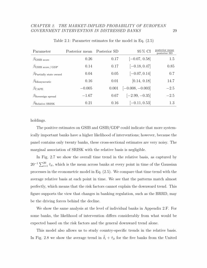
CHAPTER 2. THE MARKET-IMPLIED PROBABILITY OF EUROPEANGOVERNMENT INTERVENTION IN DISTRESSED BANKS 29
Table 2.1: Parameter estimates for the model in Eq. (2.5)
Parameter Posterior mean Posterior SD 95 % CI posterior meanposterior SD
βGSIB score 0.26 0.17 [−0.07, 0.58] 1.5
βGSIB score /GDP 0.14 0.17 [−0.18, 0.47] 0.85
βPartially state owned 0.04 0.05 [−0.07, 0.14] 0.7
βIdiosyncratic 0.16 0.01 [0.14, 0.18] 14.7
βCAPE −0.005 0.001 [−0.008,−0.003] −2.5
βSovereign spread −1.67 0.67 [−2.99,−0.35] −2.5
βRelative SRISK 0.21 0.16 [−0.11, 0.53] 1.3
holdings.
The positive estimates on GSIB and GSIB/GDP could indicate that more system-
ically important banks have a higher likelihood of interventions; however, because the
panel contains only twenty banks, these cross-sectional estimates are very noisy. The
marginal association of SRISK with the relative basis is negligible.
In Fig. 2.7 we show the overall time trend in the relative basis, as captured by
20−1∑20
i=1 τit, which is the mean across banks at every point in time of the Gaussian
processes in the econometric model in Eq. (2.5). We compare that time trend with the
average relative basis at each point in time. We see that the patterns match almost
perfectly, which means that the risk factors cannot explain the downward trend. This
figure supports the view that changes in banking regulation, such as the BRRD, may
be the driving forces behind the decline.
We show the same analysis at the level of individual banks in Appendix 2.F. For
some banks, the likelihood of intervention differs considerably from what would be
expected based on the risk factors and the general downward trend alone.
This model also allows us to study country-specific trends in the relative basis.
In Fig. 2.8 we show the average trend in δi + τit for the five banks from the United

CHAPTER 2. THE MARKET-IMPLIED PROBABILITY OF EUROPEANGOVERNMENT INTERVENTION IN DISTRESSED BANKS 30
0.0
0.1
0.2
0.3
0.4
0.5
0.6
0.7
time
rela
tive
bas
is
10/14 04/15 10/15 04/16
Figure 2.7: Average time trend in the relative basis with risk factor effects subtracted
out, 120
∑20i=1 τit, shifted to start from the observed average relative basis on September
22, 2014; posterior mean estimate (gray). Also shown is the observed average relative
basis across all banks (black). This shows that natural candidates for risk factors do
not explain the downward trend.

CHAPTER 2. THE MARKET-IMPLIED PROBABILITY OF EUROPEANGOVERNMENT INTERVENTION IN DISTRESSED BANKS 31
-0.10
-0.05
0.00
0.05
0.10
United Kingdom
time
deviation
from
trend
10/14 04/15 10/15 04/16
-0.10
-0.05
0.00
0.05
0.10
Italy
timedeviation
from
trend
10/14 04/15 10/15 04/16
-0.10
-0.05
0.00
0.05
0.10
France
time
deviation
from
trend
10/14 04/15 10/15 04/16
Figure 2.8: Time trend in the idiosyncratic deviation from the overall downward
trend, |{i ∈ country}|−1∑i∈country(δi + τit) − 120
∑20i=1 τit, for each of the countries
with three or more banks in the data set, namely the United Kingdom with five
banks, Italy with four banks, and France with three banks; posterior mean estimate
along with 68 percent credible intervals.
Kingdom, the four banks from Italy, and the three banks from France, each with the
European average subtracted out. Recently, the relative basis has declined for banks
in the United Kingdom, whereas it has increased in Italy and France. This effect
appears to be driven by declines in the relative basis at Lloyds Bank and Standard
Chartered, and, to a lesser extent, at HSBC and Royal Bank of Scotland. All the
banks in our panel saw their CDS spreads rise in the first quarter of 2016; see Fig. 2.1.
For reasons we return to later, the decline in the relative basis at these four banks from
the United Kingdom may signal a greater perceived likelihood that they would be
allowed to undergo ordinary default if their condition worsened. Standard Chartered
conducts most of its business outside the United Kingdom and may therefore be
viewed as least likely to receive government support. We discuss the effects of the
“Brexit” vote in detail in Appendix 2.G.

CHAPTER 2. THE MARKET-IMPLIED PROBABILITY OF EUROPEANGOVERNMENT INTERVENTION IN DISTRESSED BANKS 32
2.5 Evidence that Bailouts of Subordinated Debt
in Distressed Banks Have Not Become More
Likely
In this section we provide four pieces of evidence that bailouts that include subordi-
nated debt have not become more likely in distressed banks; compare the discussion
in Section 2.3.3.
2.5.1 The BRRD Legally Requires Some Bail-in Before Bailout
The BRRD, which became effective in 2016, mandates that eight percent of a bank’s
liabilities need to be bailed in before a government may inject funds. In typical cases,
this means that subordinated debt can no longer be bailed out legally. While BRRD
rules do not directly apply to Switzerland, Norway and Liechtenstein, market expec-
tations are that their national resolution frameworks will treat failing banks similarly
[Moody’s, 2015b]. Politicians and regulators may feel compelled to circumvent bailout
bans in times of stress. However, for example the discussion around troubled Italian
banks in the summer of 2016 shows that this is not trivial in the case of the BRRD
[The Economist, 2016].
2.5.2 Losses on Senior Debt Have Become More Likely Even
in Interventions
Senior bondholders tend to receive some government support in interventions; see the
discussion in Section 2.3.2. If government support for distressed banks’ bondholders
had increased so much that even the bailout of subordinated debt had become more
likely, then one would expect that governments would increasingly support senior
bondholders in interventions, too. However, we find below that the likelihood that
senior bonds would suffer in an intervention has increased. This suggests that rather

CHAPTER 2. THE MARKET-IMPLIED PROBABILITY OF EUROPEANGOVERNMENT INTERVENTION IN DISTRESSED BANKS 33
governments find themselves to be more able to impose losses on senior bondholders
recently instead of bailing them out.
To show this, we aim to identify the spread for losses on senior bonds, given an
intervention in subordinated bonds,
S(losses on senior debt | sub intervention) =.. v, (2.6)
and the spread for losses on senior bonds, given an ordinary default on subordinated
bonds,
S(losses on senior debt | sub ordinary default) =.. d. (2.7)
We cannot directly calculate these spreads the way we did for subordinated debt
in Section 2.3.1.6 Nevertheless, by making only two relatively mild assumptions, we
will be able to infer them. We begin by expressing the senior–sub ratio from (2.4) as
the sum of loss severity in an intervention and loss severity in an ordinary default,
weighted with the respective conditional probability:
CDS2014senior
CDS2014= S(losses on senior debt | sub intervention) (2.8)
× P(sub intervention | any sub 2014 credit event)
+ S(losses on senior debt | sub ordinary default)
× P(sub ordinary default | any sub 2014 credit event).
We also express
P(sub intervention | any sub 2014 credit event) (2.9)
=relative basis
w=
1
w
CDS2014 − CDS2003
CDS2014,
6This is because ISDA made a change to senior CDS definitions in 2014 that is not related to
intervention: it removed the sub–senior cross trigger. While a senior 2003 CDS triggers whenever a
subordinated 2003 CDS triggers, a senior 2014 CDS will trigger only in case of an event that directly
affects senior debt. This decreases the value of a senior 2014 CDS, and has no effect on subordinated
CDS.

CHAPTER 2. THE MARKET-IMPLIED PROBABILITY OF EUROPEANGOVERNMENT INTERVENTION IN DISTRESSED BANKS 34
and we know that
P(sub ordinary default | any sub 2014 credit event) (2.10)
= 1− P(sub intervention | any sub 2014 credit event).
To understand the role of w, consider the simplified representation of the relative
basis
CDS2014 − CDS2003
CDS2014
=Lsub intervention P(sub intervention)
Lsub intervention P(sub intervention) + Lordinary default P(ordinary default)
= w P(sub intervention | any sub 2014 credit event).
From
w−1 = P(sub intervention | any sub 2014 credit event) (2.11)
+Lsub ordinary default
Lsub intervention
P(sub ordinary default | any sub 2014 credit event)
we see that w is increasing in the ratio of loss given an intervention and loss given an
ordinary default, and that w equals one if the conditional losses are equal.
Plugging (2.9) and (2.10) into Eq. (2.8) yields, for each bank i and point in time t,
CDS2014senior it
CDS2014it
=vitwit
CDS2014it − CDS2003
it
CDS2014it
− ditwit
CDS2014it − CDS2003
it
CDS2014it
+ dit. (2.12)
This is an underdetermined system of equations. We make two assumptions to ensure
identifiability.
Assumption 1. Values for v that are close in time are similar to each other. Likewise,
values for d that are close in time are similar.
We make this assumption precise further below.
Assumption 2. wit changes linearly with time, separately for each bank.

CHAPTER 2. THE MARKET-IMPLIED PROBABILITY OF EUROPEANGOVERNMENT INTERVENTION IN DISTRESSED BANKS 35
This assumption is needed because, locally in time, the separate effects of vit and
wit are only weakly identifiable. This assumption is far weaker than assuming, for
example, that all conditional losses are equal. Under Assumption 2, the conditional
losses of intervention and ordinary default may be different, and they may even differ
across banks and, linearly, over time.
We obtain estimates for the vit = S(losses on senior debt | sub intervention)it from
Eq. (2.6) as well as the dit = S(losses on senior debt | sub ordinary default)it from (2.7)
by expressing (2.12) as a regression model, with an error term εit. We incorporate
Assumptions 1 and 2 in this regression model by placing so-called random walk priors
on vit/wit and dit, and allowing wit to change linearly over time for each bank. We
discuss the details of the prior and hyperprior specification and of the Markov chain
Monte Carlo sampling in Appendix 2.C.2.
Fig. 2.9 shows the averages for S(losses on senior debt | sub bail-in) and also the
averages for S(losses on senior debt | sub ordinary default) over time. We see that the
market implies that an ordinary default typically involves larger losses on senior debt
than an intervention, with average spreads of 0.60 and 0.39, respectively. We show
the results separately for each bank in Fig. 2.12 in Appendix 2.H. The average spread
for losses on senior debt given sub ordinary default is approximately constant over
time at a high level. This suggests that the market has not become more nervous
about disruptions in an ordinary default scenario. The average spread for losses on
senior debt given sub intervention is lower, but surprisingly large, and it has increased
considerably. This means that the market expects that governments have become
less likely to support senior creditors in an intervention, and that the current levels
of subordinated debt do not suffice to cover the expected losses in an intervention.

CHAPTER 2. THE MARKET-IMPLIED PROBABILITY OF EUROPEANGOVERNMENT INTERVENTION IN DISTRESSED BANKS 36
losses on senior debt | sub ordinary default
losses on senior debt | sub intervention
0.0
0.2
0.4
0.6
time
spre
ad
10/14 04/15 10/15 04/16
Figure 2.9: Average of S(losses on senior debt | sub ordinary default) as well as
S(losses on senior debt | sub intervention) over time; posterior mean estimate along
with 68 percent credible intervals. These spreads function as weights in (2.8). The fig-
ure shows that S(losses on senior debt | sub intervention) increased slightly over time,
and the other spread stayed roughly constant.

CHAPTER 2. THE MARKET-IMPLIED PROBABILITY OF EUROPEANGOVERNMENT INTERVENTION IN DISTRESSED BANKS 37
2.5.3 Relationship between Relative Basis and Likelihood of
Bailout
If bailouts that include subordinated debt had been replacing interventions system-
atically, then we should observe a strong negative correlation between the relative
basis and the conditional likelihood of bailout of subordinated debt. This is because
a shift of probability mass from interventions to bailouts that include subordinated
debt reduces the relative basis. However, we find in the following that the correlation
is weak.
The conditional likelihood of a bailout that includes subordinated debt is
S(bailout incl sub debt | distress) (2.13)
= 1− S(ordinary default ∪ intervention)
S(ordinary default ∪ intervention ∪ bailout incl sub debt).
We cannot measure (2.13) directly because the spread that includes full bailout,
S(ordinary default ∪ intervention ∪ bailout incl sub debt), is not observable in the
market. However, we can use Moody’s KMV model to estimate a bank-specific spread
that includes bailouts of subordinated debt. This is possible because the KMV model
includes bailout as a default event, and because it uses the counterfactual that losses
in a bailout of subordinated debt are not zero but the average for interventions or
ordinary defaults.
A complication is that the KMV model estimates a spread calculated under the
real-world measure, Sphysical(ordinary default∪ intervention∪bailout incl sub debt) =
Lphysicaldistress · Pphysical(distress). In contrast, a spread S is market implied, which means
that it can be expected to include a risk premium. We address this issue further
below.
We obtain annualized five-year estimates of Pphysical(distress) for all banks and
points in time from Moody’s KMV CreditEdge model, which is based on the general
approach of Merton [1974]. Although the approach of Merton [1974] generates a risk
neutral probability of distress, KMV CreditEdge is calibrated to match historical

CHAPTER 2. THE MARKET-IMPLIED PROBABILITY OF EUROPEANGOVERNMENT INTERVENTION IN DISTRESSED BANKS 38
distress probabilities and is therefore under the physical measure. The real-world
default probability estimates range from significantly less than 0.01 for banks such as
UBS, Lloyds Bank and HSBC up to above 0.08 for Banca Monte dei Paschi di Siena.
We also obtain estimates of the annualized five-year real-world expected loss given
default for subordinated debt, Lphysicaldistress , from Moody’s KMV LossCalc model. Loss-
Calc is a regression model that uses historical data on recoveries together with pre-
dictors such as industry, credit cycle stage, debt type, and the probability of distress.
In LossCalc a bailout event is assigned losses that would be expected under a distress
that is not a bailout [Moody’s Analytics, 2016]. The estimates for the loss given
distress on subordinated bonds, Lphysicaldistress , show relatively little variation across banks
and time around their mean of 80 percent. This relatively high number means that
distress would typically wipe out most of a bank’s subordinated debt.
We now investigate the correlation between the conditional likelihood of bailout
that includes subordinated debt and the relative basis. As discussed at the beginning
of this analysis, if bailouts that include subordinated debt had systematically replaced
interventions, then this correlation should be strongly negative. We cannot directly
plug the estimates from the KMV model for Sphysical(ordinary default∪ intervention∪bailout incl sub debt) into (2.13), because then we would be subtracting market-
implied from real-world spreads. Instead, we define
b =Sphysical(ordinary default ∪ intervention ∪ bailout incl sub debt)
S(ordinary default ∪ intervention)(2.14)
=Lphysicaldistress · Pphysical(distress)
CDS2014.
This quantity takes a large value when the probability of bailout that includes sub
debt is high and/or the risk premium is low, and it takes a small value when the
probability of such a bailout is low and/or the risk premium is high (recall that the
KMV physical probabilities treat bailouts as defaults). Empirically, we find that b is
typically much smaller than one, with average values for the banks ranging from 0.29
for UBS and 0.32 for Banco Comercial Portugues to 0.98 for Societe Generale and

CHAPTER 2. THE MARKET-IMPLIED PROBABILITY OF EUROPEANGOVERNMENT INTERVENTION IN DISTRESSED BANKS 39
1.02 for Commerzbank, with a mean across all banks of 0.68.
We address the complication that b also depends on the risk premium by taking, for
each bank, the average value of b over time, which marginalizes out this dependency.
Likewise, we calculate the average relative basis over time, separately for each bank.
We find that the empirical correlation between the bank-averages for b and the
bank-averages for the relative basis is 0.02. Given the small sample size of only twenty
banks, the uncertainty about the true correlation is relatively high, as captured by
a 95 percent confidence interval that ranges from −0.43 to 0.46. Hence, we also
perform correlation analyses with the panel data in Appendix 2.I. Both within and
across time series we find only a very small negative correlation on average. This
suggests that bailouts that include subordinated debt have not systematically replaced
interventions.
2.5.4 Rating Agencies Removed or Lowered Uplift for Gov-
ernment Support in Bank Bond Ratings
Rating agencies have eliminated their ratings uplift on all junior instruments in expec-
tation of reduced government support for such instruments following recent changes in
banking regulation; see, for example, Moody’s [2015a] and Standard & Poor’s [2015].
This development is consistent with our interpretation of the decline in the relative
basis as reflecting reduced expectations of government support.
2.6 Conclusion
The European Union has formalized the role of bond bail-in in resolving distressed
banks through the BRRD. Contemporaneously, ISDA has introduced new definitions
for the CDS market in 2014 to cope with the complications surrounding bond bail-in.
Using data of CDS trading under old and new ISDA definitions, we find reduced
market expectations of support for senior bondholders in bank failures where at most

CHAPTER 2. THE MARKET-IMPLIED PROBABILITY OF EUROPEANGOVERNMENT INTERVENTION IN DISTRESSED BANKS 40
senior bondholders, but not subordinated bondholders, receive a bailout.
We have provided evidence that bailouts that include subordinated debt have
not become more likely conditionally over the same time horizon; this suggests that
expectations of government support for banks in distress have decreased. We have
furthermore provided evidence that natural candidates for risk factors cannot explain
the highly synchronized downward trend in the relative basis; this leaves changes in
banking regulation as the likely cause.
We conclude from these findings that changes in European banking regulation,
such as the BRRD, have reduced expectations of government support for ailing banks.
This development represents important progress in the credibility of financial reforms
aimed at reducing perceived government guarantees for large banks.

CHAPTER 2. THE MARKET-IMPLIED PROBABILITY OF EUROPEANGOVERNMENT INTERVENTION IN DISTRESSED BANKS 41
Appendix to Chapter 2
2.A Description of the CDS Quote Data
We consider subordinated five-year 2003 and 2014 CDS spreads, starting on Sept. 22,
2014, the date of the introduction of the 2014 CDS, to April 18, 2016. These data are
from Markit, and we already used them in Fig. 2.1. For many of the smaller European
banks, subordinated CDS are traded too rarely to give good weekly, or even daily,
spread quotes. We select only banks for which subordinated data quality is judged
“B” or higher — indicating at least moderate data quality — according to Markit’s
data quality rating on at least 95 percent of quote days (which include some public
holidays). Markit judges data quality by the number of sources that provide spread
quotes, as well as competitiveness, liquidity and transparency of the market. We are
left with twenty banks that satisfy this data quality requirement; their names are
given in Fig. 2.10. Only on a very few days their data quality falls below “B.” Data
quality is highly similar for subordinated 2003 and 2014 CDS, across all banks —
even those banks that are not included in our final data set because of insufficient
data quality. This suggests that our sampling according to the data quality rating is
outcome-independent.
For senior CDS, 85 percent of quoted spreads have a Markit data quality rating
of “AA” or “A,” and only 0.3 percent are rated less than “B.”
We confirm that for these banks quoted spreads from Markit closely match spreads
at which actual trades happen in Appendix 2.B, using anonymized data of actual CDS
trades confirmed through The Depository Trust & Clearing Corporation (DTCC).
Lastly, we subsample the panel data to a weekly frequency to reduce the effect of
potential short term autocorrelation in Markit’s spread quotes.

CHAPTER 2. THE MARKET-IMPLIED PROBABILITY OF EUROPEANGOVERNMENT INTERVENTION IN DISTRESSED BANKS 42
We note that the CDS market is somewhat technically driven, because CDS can
be used to both hedge against default, and to hedge against the spread of other CDS,
bonds or counterparty exposures. Hedging spread changes with subordinated 2003
CDS may be perceived as slightly cheaper than hedging with 2014 CDS. At the same
time, switching from old 2003 CDS to new 2014 CDS may cause wide bid–ask spreads
during the time of transition. We find in Section 2.3.2 that neither of these technical
factors has a large impact on the quotes we study.
2.B Establishing Quote Validity
Our analysis uses quoted rather than transacted spreads. While these quotes are not
tradable, they are a composite of tradable quotes submitted by market makers in
European financial reference entities. As market makers have been known to shade
surveys to favor their own interests, for example in the recent LIBOR scandal, we
seek to verify that the quotes are accurate indicators of the spreads at which trades
will occur.
We obtained anonymized data of CDS trades recorded by The Depository Trust
& Clearing Corporation (DTCC). These are all trades where at least one of the coun-
terparties is based in the United States. We consider transactions that occur between
September 1, 2014 and February 12, 2016. We focus in our sample on confirmed
initial trades which reference subordinated debt and are roughly five years at incep-
tion. In other words, we exclude canceled transactions, as the information content
of those may be misleading. We also ignore other DTCC transaction classifications
such as Assignment, Amendment, Backload, Exit, Increase, and Terminate because
these transactions largely embed information that follow trade inception. As we aim
to compare information content from transaction execution to market quotes, only
initial trades are relevant.
We do not expect quoted spreads and transacted spreads to align perfectly for sev-

CHAPTER 2. THE MARKET-IMPLIED PROBABILITY OF EUROPEANGOVERNMENT INTERVENTION IN DISTRESSED BANKS 43
eral reasons. First among these are differences in upfront payment conventions. Typ-
ically, the upfront of a CDS contract reflects the difference between market spreads
and a fixed coupon spread the contract pays. To the extent the upfront is higher, the
fair value spread will be lower. Sometimes, market participants transact an upfront
different than the one that reflects this difference in spreads. We delete trades where
we can observe intentional deviations from the market price, specifically those trades
whose fair value spreads are exactly 100, 300 and 500 basis points. Additional sources
of discrepancy between market quoted spread and transacted spread are differences
in contract maturities, choice of nonstandard coupon payment and swap termination
dates, nonstandard transaction sizes, and adjustments for counterparty risk since the
market is over the counter and not anonymous. To address these issues, we standard-
ize market-quoted maturities to correspond to those of each contract and assume that
each CDS terminates on the International Money Market (IMM) date closest before,
or upon, the transacted termination date. We ensure that each transaction’s base
currency, seniority, and documentation clause take the same value for each quote.
We obtain, for each bank i and point in time t the transacted spread, sji,t, and the
quoted spread, qji,t, where we use j to denote that there may be multiple trades for a
bank on a given day. We model the transacted spread–quoted spread relationship as
linear, with error term εji,t:
sji,t = α0 + β0qji,t + εji,t. (2.15)
We run this regression independently four times: for subordinated 2003 CDS, for
subordinated 2014 CDS, for senior 2003 CDS, and senior 2014 CDS. We show the
estimation results in Table 2.2. We find a strong relationship between same day
quotes and transacted prices. The coefficient of determination is high or very high in
all of the regressions. The estimated slopes on the quoted spreads are close to one.
That the sample size is relatively low for subordinated 2003 CDS reflects that they
are less frequently traded. At the same time, Markit obtains quotes from all dealers,
whereas DTCC coverage is limited to trades in which at least one counterparty is

CHAPTER 2. THE MARKET-IMPLIED PROBABILITY OF EUROPEANGOVERNMENT INTERVENTION IN DISTRESSED BANKS 44
Table 2.2: Assessing the relationship between traded spreads and quoted spreads
Regression 1 Regression 2 Regression 3 Regression 4
Traded sub 2003 spread Traded sub 2014 spread Traded senior 2003 spread Traded senior 2014 spread
Slope on quoted spread 1.05 1.05 1.02 1.05
(0.08) (0.00) (0.01) (0.00)
Intercept 0.10 0.25 0.01 0.21
(0.37) (0.01) (0.07) (0.00)
Sample size 81 3139 287 5905
Coefficient of determination 0.67 0.99 0.94 0.99
(standard errors in parentheses)
based in the United States. Another reason that Markit assesses data quality for
subordinated 2003 CDS for the twenty banks we study as high could be that many
dealers are willing to quote 2003 subordinated CDS spreads (high liquidity), but only
few, potentially nonstandard, trades are executed.
2.C Prior and Hyperprior Distributions and Sam-
pling Diagnostics
We now discuss the choice of prior and hyperprior distributions as well as the details
of the Markov chain Monte Carlo sampling for the regression models in Sections 2.4.2
and 2.5.2.
2.C.1 Model in Eq. (2.5) in Section 2.4.2
As the prior distributions we choose:
α ∼ normal(0, 1),
δii.i.d.∼ normal(0, σ2
δ ),
β ∼ normal(0, diag(52)),
(τi1, . . . , τiT )i.i.d.∼ GP(0, k),
εiti.i.d.∼ normal(0, σ2).

CHAPTER 2. THE MARKET-IMPLIED PROBABILITY OF EUROPEANGOVERNMENT INTERVENTION IN DISTRESSED BANKS 45
Here GP(0, k) denotes a Gaussian process prior that has zero mean and covariance
function
k(a, b) = η2 exp(−(a− b)2/ρ2).
For a reference on Gaussian processes priors, see Rasmussen and Williams [2006].
The parameter η controls the variation of the Gaussian process, which cannot be
large because of the boundedness of the relative basis. The parameter ρ controls the
average length scale of the process, here in weeks due to the subsampling. We set the
prior standard deviation for the elements of β to five because a change in sovereign
spread of one percent likely does not result in a change in the relative basis of much
more than five percent. Since government spread is measured on the smallest scale
by far, it likely also has the largest regression coefficient.
We choose the following hyperprior distributions:
σ ∼ half-Cauchy(0, 0.1),
σδ ∼ half-Cauchy(0, 0.1),
η2 ∼ half-Cauchy(0, 0.1),
ρ2 ∼ half-Cauchy(0, 100).
Here we set a prior mean absolute deviation for the noise level σ and the random effects
standard deviation σδ of 0.1, considering that the relative basis itself is approximately
lower-bounded at 0 and that it cannot exceed 1. Half-Cauchy prior distributions are
generally recommended as priors on standard deviations or variances in hierarchical
models, for example in Gelman [2006].
We draw Markov-Chain Monte Carlo samples from the posterior distribution using
the No-U-Turn sampler [Hoffman and Gelman, 2014], a variant of Hamiltonian Monte
Carlo, implemented in the software Stan [Stan Development Team, 2015]. For each of
15 separate chains, we draw 2,500 samples following a burn-in phase of 2,500 samples,
for a total of 37,500 Monte Carlo samples. We check that after warm-up the chains
have converged to their stationary distribution using the statistic R [Brooks and

CHAPTER 2. THE MARKET-IMPLIED PROBABILITY OF EUROPEANGOVERNMENT INTERVENTION IN DISTRESSED BANKS 46
Gelman, 1998]; it takes a value of less than 1.1 for all parameters, which indicates
good mixing of the Markov chains. For each parameter, the effective sample size
drawn is greater than 100, and typically much larger than that. For all parameters the
posterior distribution is significantly more concentrated than the prior distribution,
in an area of the parameter space that is likely under the prior, which implies that
the prior distributions did not influence the inferences in any meaningful way.
2.C.2 Model in Section 2.5.2
We place the priors
εiti.i.d.∼ normal(0, σ2),
vitwit| vi(t−1)wi(t−1)
i.i.d.∼ normal(vi(t−1)wi(t−1)
, σ2v/w), with
vitwit≥ 0, for all i, and t = 2, . . . , T,
(2.16)
dit | di(t−1) i.i.d.∼ normal(di(t−1), σ2d), with dit ≥ 0, for all i, and t = 2, . . . , T
(2.17)
wit =T − tT − 1
wi1 +t− 1
T − 1wiT , with wit ≥ 0, for all t = 2, . . . , T − 1.
Here (2.16) and (2.17) are so-called random walk priors, which limit the size of jumps
between adjacent values. As hyperprior distributions for σ, σv/w, σd and σw we place
independent half-Cauchy(0,1) distributions.
We draw 2,500 Markov-chain Monte Carlo samples each using five chains, following
a burn-in phase of equal length, for a total sample size of 12,500. The effective sample
size for each of the parameters is at least in the hundreds. The statistic R takes a
value close to 1, which indicates very good mixing of the Markov chains. The effect
of the positivity constraints is limited.

CHAPTER 2. THE MARKET-IMPLIED PROBABILITY OF EUROPEANGOVERNMENT INTERVENTION IN DISTRESSED BANKS 47
2.D Raw global systemically important bank (GSIB)
Score and Partial State Ownership
Table 2.3 shows each bank’s raw GSIB score and whether it is partially state owned,
as discussed in Section 2.4.2. The raw GSIB scores are our own calculations based on
the banks’ disclosure reports for globally financially important institutions in 2014.
Banco Comercial Portugues and Banco Popolare do not make these reports publicly
available. We impute their raw GSIB score using a linear regression with total risk-
weighted assets as the predictor.
2.E Hyperparameter Estimates for the Model in
Equation (2.5) in Section 2.4.2
The hyperparameter estimation results are in Table 2.4. All credible intervals contain
the mode of the distribution. The lower bounds of the credible intervals for the
random intercepts standard deviation and for the Gaussian process variation are
considerably above zero, which suggests that level differences persist in the relative
basis across banks, but that levels also change over time. The Gaussian process
lengthscale of roughly six weeks indicates that the relative basis does typically not
undergo rapid level changes.
2.F The Observed and Predicted Relative Basis
for Individual Banks
Fig. 2.10 shows how much a given bank’s spread for an intervention deviates from what
would be expected based on the risk factors and the overall downward trend alone. We
include the overall downward trend because it may be explained by changes in banking

CHAPTER 2. THE MARKET-IMPLIED PROBABILITY OF EUROPEANGOVERNMENT INTERVENTION IN DISTRESSED BANKS 48
Tab
le2.
3:E
ach
ban
k’s
orig
in,
raw
GSIB
scor
e,m
ean
idio
syncr
atic
stre
ssan
dm
ean
rela
tive
SR
ISK
,as
defi
ned
in
Sec
tion
2.4.
2.
Ban
kC
ountr
yR
awG
SIB
scor
eM
ean
idio
syncr
atic
stre
ssM
ean
rela
tive
SR
ISK
Bar
clay
sB
ank
plc
Unit
edK
ingd
om34
9−
0.3
0.10
Ban
caM
onte
dei
Pas
chi
di
Sie
na
SpA
Ital
y22
1.1
0.01
Ban
coB
ilbao
Viz
caya
Arg
enta
ria
SA
Spai
n90
0.0
0.02
Ban
coC
omer
cial
Por
tugu
esSA
Por
tuga
l45∗
1.1
0.00
Ban
coP
opol
are
SC
Ital
y47∗
0.6
0.01
Ban
coSan
tander
SA
Spai
n20
80.
00.
05
BN
PP
arib
asF
rance
405
−0.
40.
12
Com
mer
zban
kA
GG
erm
any
107
0.1
0.03
Cre
dit
Agr
icol
eSA
Fra
nce
186
−0.
30.
11
Cre
dit
Suis
seG
pA
GSw
itze
rlan
d27
0−
0.3
0.04
Deu
tsch
eB
ank
AG
Ger
man
y36
00.
00.
11
HSB
CB
ank
plc
Unit
edK
ingd
om43
8−
0.4
0.05
ING
Ban
kN
VN
ether
lands
132
−0.
40.
04
Inte
saSan
pao
loSpA
Ital
y80
0.0
0.02
Llo
yds
Ban
kplc
Unit
edK
ingd
om76
−0.
40.
03
Roy
alB
ank
ofSco
tlan
dplc
Unit
edK
ingd
om21
3−
0.2
0.06
Soci
ete
Gen
eral
eF
rance
210
−0.
20.
08
Sta
ndar
dC
har
tere
dB
ank
Unit
edK
ingd
om14
20.
00.
03
UB
SA
GSw
itze
rlan
d18
9−
0.3
0.02
UniC
redit
SpA
Ital
y16
50.
30.
05
∗im
pute
d

CHAPTER 2. THE MARKET-IMPLIED PROBABILITY OF EUROPEANGOVERNMENT INTERVENTION IN DISTRESSED BANKS 49
Table 2.4: Hyperparameter estimates for the model in Eq. (2.5)
Parameter Posterior mean Posterior SD 95 % CI
σδ (random intercepts SD) 0.08 0.02 [0.05, 0.11]
η (GP variation) 0.07 0.003 [0.06, 0.07]
ρ (GP lengthscale) 6.2 0.2 [5.8, 6.7]
σ (noise SD) 0.013 0.0003 [0.013, 0.014]
regulation. We find that the two Swiss banks show the most striking deviations from
what the model would predict based on the risk factors alone. UBS has a surprisingly
high relative basis throughout the whole period — and therefore is unexpectedly likely
to experience a intervention if it were to enter distress without being bailed out. For
Credit Suisse, the relative basis starts out similarly high but market expectations
have changed drastically, such that its relative basis is now near zero — suggesting
that, if Credit Suisse were to enter distress without receiving a bailout, it would most
likely undergo ordinary default. Also for Banco Comercial Portugues, the relative
basis is unexpectedly low, suggesting a high likelihood of ordinary default, if it were
to enter distress and not receive a bailout.
These persistent idiosyncratic deviations occur even though our model in (2.5)
accounts for traditional measures of systemic importance, such as SRISK and GSIB
score. This suggests that whether a government decides to take action on a distressed
bank depends on strongly idiosyncratic factors or unobserved political factors, which
are not captured by traditional measures of systemic importance.
2.G Case Study: “Brexit” Vote
The United Kingdom voted on June 23, 2016 to leave the European Union. The vote
came as a surprise, with most polls before voting day suggesting a narrow win for

CHAPTER 2. THE MARKET-IMPLIED PROBABILITY OF EUROPEANGOVERNMENT INTERVENTION IN DISTRESSED BANKS 50
0.0
0.2
0.4
0.6
Barclays
time
relative
basis
10/14 07/15 04/16
0.0
0.2
0.4
0.6
Monte dei Paschi
time
relative
basis
10/14 07/15 04/16
0.0
0.2
0.4
0.6
BBVA
time
relative
basis
10/14 07/15 04/16
0.0
0.2
0.4
0.6
B C Portugues
time
relative
basis
10/14 07/15 04/16
0.0
0.2
0.4
0.6
Bco Popolare
time
relative
basis
10/14 07/15 04/16
0.0
0.2
0.4
0.6
Santander
time
relative
basis
10/14 07/15 04/16
0.0
0.2
0.4
0.6
BNP Paribas
time
relative
basis
10/14 07/15 04/16
0.0
0.2
0.4
0.6
Commerzbank
time
relative
basis
10/14 07/15 04/16
0.0
0.2
0.4
0.6
Cr Agricole
time
relative
basis
10/14 07/15 04/16
0.0
0.2
0.4
0.6
Credit Suisse
time
relative
basis
10/14 07/15 04/16
0.0
0.2
0.4
0.6
Deutsche Bk
time
relative
basis
10/14 07/15 04/16
0.0
0.2
0.4
0.6
HSBC
time
relative
basis
10/14 07/15 04/16
0.0
0.2
0.4
0.6
ING
time
relative
basis
10/14 07/15 04/16
0.0
0.2
0.4
0.6
Intesa
time
relative
basis
10/14 07/15 04/16
0.0
0.2
0.4
0.6
Lloyds Bk
time
relative
basis
10/14 07/15 04/16
0.0
0.2
0.4
0.6
R B of Scotland
time
relative
basis
10/14 07/15 04/16
0.0
0.2
0.4
0.6
Societe Generale
time
relative
basis
10/14 07/15 04/16
0.0
0.2
0.4
0.6
Std Chartered
time
relative
basis
10/14 07/15 04/16
0.0
0.2
0.4
0.6
UBS
time
relative
basis
10/14 07/15 04/16
0.0
0.2
0.4
0.6
UniCredit
time
relative
basis
10/14 07/15 04/16
Figure 2.10: Time trend in the model predictions, α+βT (risk factors)it+120
∑20j=1 τjt,
(gray, posterior mean estimate, along with 68 percent credible intervals) and the ob-
served relative basis (solid), for each bank. We include the overall downward trend
because it may be explained with changes in banking regulation. We exclude the indi-
vidual random effects and Gaussian process estimates, since these capture systematic
but unexplained variation.

CHAPTER 2. THE MARKET-IMPLIED PROBABILITY OF EUROPEANGOVERNMENT INTERVENTION IN DISTRESSED BANKS 51
“remain.” This provides a rare opportunity for us to observe the market reaction to
expected changes in governmental policy.
2014 spreads increased strongly for all banks, with an average of 16 percent (log
difference between average of two weeks before and average of two weeks following
the Brexit vote). This is in line with the strong decline in European stock markets,
and the fall of the British Pound after the Brexit vote. We assess how unusual an
increase in spreads of this size is by comparing it with all other changes over a time
horizon of same length between September 2014 and August 2016. We find that
spreads increased more strongly than around the Brexit vote only in six percent of
other time windows of the same width.
The relative basis increased only slightly around the Brexit vote, with an average of
three percent (again using log differences over the same time window as above). This
means that the market does not expect for Brexit to, on average, have a significant
change on governmental policy regarding distressed banks. However, we find that
banks that generate a large share of their income (2015 numbers) inside the United
Kingdom have a higher increase in their relative basis; see Table 2.5 for a comparison
of geographical income source and change in relative basis. For example, the log
difference in the relative basis for Lloyds Bank, which generates nearly all of its
income inside the United Kingdom, is a very large 23 percent. This suggests that
government support has increased in the United Kingdom for banks that are truly
dependent on the home market.
Fig. 2.11 shows a strong correlation of 0.61 between changes in 2014 spreads and
changes in the relative basis around Brexit. This high correlation may suggest that
banks that are affected by Brexit are expected to have increased government support.
The correlation is stronger than the correlation observed in 88 percent of comparable
time windows in our data set.

CHAPTER 2. THE MARKET-IMPLIED PROBABILITY OF EUROPEANGOVERNMENT INTERVENTION IN DISTRESSED BANKS 52
Table 2.5: United Kingdom income as share of total income for banks in the United
Kingdom, and relative change in the relative basis around the Brexit vote
Bank UK income share relative change in relative basis
Standard Chartered < 5 % −5 %
HSBC 26 % 11 %
Barclays 48 % 8 %
Royal Bank of Scotland 88 % 11 %
Lloyds Bank 95 % 23 %
0.00 0.05 0.10 0.15 0.20 0.25 0.30
-0.1
0.0
0.1
0.2
0.3
relative change in 2014 spread
rela
tive
chan
gein
rela
tive
bas
is
Monte dei Paschi
BBVA
B C Portugues
Bco Popolare
Santander
BNP Paribas
Commerzbank
Cr Agricole
Credit Suisse
Deutsche BkING
IntesaSocGen
UBS
UniCredit
Barclays
HSBC
Lloyds Bk
R B of Scotland
Std Chartered
Figure 2.11: Relative change in 2014 spread and relative change in relative basis
around the “Brexit” vote. Banks from the United Kingdom are in boldface. Each
gray line is the respective average of the changes of all banks.

CHAPTER 2. THE MARKET-IMPLIED PROBABILITY OF EUROPEANGOVERNMENT INTERVENTION IN DISTRESSED BANKS 53
2.H Additional Figures
Fig. 2.12 shows for each bank over time S(losses on senior debt | sub ordinary default)
and also S(losses on senior debt | sub intervention), otherwise discussed in Section 2.5.2.
For most banks the spreads have stayed approximately constant. Exceptions are
Credit Suisse and Banco Comercial Portugues, for which the market implies in the
summer of 2016 that both an intervention and an ordinary default would hit senior
bonds unusually strongly, and Banca Monte dei Paschi di Siena, for which the market
implies that an intervention would likely not hit senior bonds, if these banks were to
enter distress without receiving a bailout.
2.I Time Series Relationship between Relative Ba-
sis and Conditional Likelihood of Subordinated
Debt Bailout
In Section 2.5.3 we find cross-sectional evidence that bailouts that include subordi-
nated debt do not crowd out interventions. In the following we analyze the association
over time between how likely a bank is to be bailed in and how likely it is to receive
a bailout. We will conduct this analysis on a relative scale, to remove the shared
influence of a potentially time-varying risk premium.
The empirical correlation of the average trend in the empirical bit from Eq. (2.14)
with CAPE, discussed in Section 2.4.2, is 0.61; this suggests that the trend is to
a large extent explained by changes in the risk premium, and not changes in the
probability of bailouts that include subordinated debt.
We normalize bit with respect to the average trend:
bnormalizedit =
bit
20−1∑20
i=1 bit.
This quantity is independent of any shared risk premium across banks, but also

CHAPTER 2. THE MARKET-IMPLIED PROBABILITY OF EUROPEANGOVERNMENT INTERVENTION IN DISTRESSED BANKS 54
0.0
0.2
0.4
0.6
0.8
Barclays
time
spread
10/14 07/15 04/16
0.0
0.2
0.4
0.6
0.8
Monte dei Paschi
timespread
10/14 07/15 04/16
0.0
0.2
0.4
0.6
0.8
BBVA
time
spread
10/14 07/15 04/16
0.0
0.2
0.4
0.6
0.8
B C Portugues
time
spread
10/14 07/15 04/16
0.0
0.2
0.4
0.6
0.8
Bco Popolare
time
spread
10/14 07/15 04/16
0.0
0.2
0.4
0.6
0.8
Santander
time
spread
10/14 07/15 04/16
0.0
0.2
0.4
0.6
0.8
BNP Paribas
timespread
10/14 07/15 04/16
0.0
0.2
0.4
0.6
0.8
Commerzbank
time
spread
10/14 07/15 04/16
0.0
0.2
0.4
0.6
0.8
Cr Agricole
time
spread
10/14 07/15 04/16
0.0
0.2
0.4
0.6
0.8
Credit Suisse
time
spread
10/14 07/15 04/16
0.0
0.2
0.4
0.6
0.8
Deutsche Bk
time
spread
10/14 07/15 04/16
0.0
0.2
0.4
0.6
0.8
HSBC
timespread
10/14 07/15 04/16
0.0
0.2
0.4
0.6
0.8
ING
time
spread
10/14 07/15 04/16
0.0
0.2
0.4
0.6
0.8
Intesa
time
spread
10/14 07/15 04/16
0.0
0.2
0.4
0.6
0.8
Lloyds Bk
time
spread
10/14 07/15 04/16
0.0
0.2
0.4
0.6
0.8
R B of Scotland
time
spread
10/14 07/15 04/16
0.0
0.2
0.4
0.6
0.8
Societe Generale
time
spread
10/14 07/15 04/16
0.0
0.2
0.4
0.6
0.8
Std Chartered
time
spread
10/14 07/15 04/16
0.0
0.2
0.4
0.6
0.8
UBS
time
spread
10/14 07/15 04/16
0.0
0.2
0.4
0.6
0.8
UniCredit
time
spread
10/14 07/15 04/16
Figure 2.12: Individual trends in S(losses on senior debt | sub ordinary default) (top
solid line, posterior mean estimate along with 68 percent credible intervals) as well as
S(losses on senior debt | sub intervention) (bottom solid line, posterior mean estimate
along with 68 percent credible intervals); also shown are the respective averages across
all banks (top and bottom dotted line).

CHAPTER 2. THE MARKET-IMPLIED PROBABILITY OF EUROPEANGOVERNMENT INTERVENTION IN DISTRESSED BANKS 55
independent of any common trend in the bit that could be attributed to changes
in the bailout probability. This measure tells us how likely bailout that includes
subordinated debt is for a given bank i, relative to how likely bailout that includes
subordinated debt is on average for all other banks in our data set, at a given point
in time. By construction, its average at each point in time is one.
Similarly, we normalize the relative basis to remove any aggregate trend from it:
normalized relative basisit =relative basisit
20−1∑20
i=1 relative basisit.
The normalized relative basis measures how likely intervention is for a given bank i,
relative to how likely intervention is on average for all other banks, at a given point
in time.
We find that the empirical correlation between the empirical bnormalizedit and the
normalized relative basis is 0.02. This means that firms with a larger than average
conditional chance of intervention have no tendency to also have a larger than average
conditional chance of bailout that includes subordinated debt. We also analyze,
separately for each bank, the empirical correlation between changes over time in the
empirical bnormalizedit and changes over time in the normalized relative basis. We find
these correlations between changes to range from −0.42 to 0.035, with a mean of
−0.25, which is consistent with at most a slight tendency for bailouts that include
subordinated debt to crowd out interventions.

CHAPTER 3. ESTIMATING A COVARIANCE MATRIX FOR MARKET RISKMANAGEMENT 56
Chapter 3
Estimating a Covariance Matrix
for Market Risk Management and
the Case of Credit Default Swaps
This chapter is based on a manuscript of the same title, authored by Richard Neuberg
and Paul Glasserman. It is available at SSRN 2782107.
3.1 Introduction
Covariance matrices of asset returns are at the core of risk management and modern
portfolio theory. However, their estimation is difficult, because, even if covariances
are assumed constant over time, these matrices have p(p+1)/2 free parameters, where
p is the number of financial assets, which may be larger than the available sample
size. Sample covariance matrices often perform poorly out-of-sample, since they may
not even be of full rank. Traditionally, the problem with sample covariance matrices
is overcome by using single- or multi-factor factor models, which link observed asset
returns to a few observed or latent factors. For a review, see Bai and Shi [2011].
Factor models are easily interpretable. However, they, too, might not be optimal

CHAPTER 3. ESTIMATING A COVARIANCE MATRIX FOR MARKET RISKMANAGEMENT 57
for estimating a covariance matrix for a specific market risk management purpose:
we show that latent factor models systematically misestimate the variance of certain
portfolios.
For market risk management, which is our focus in this article, a covariance matrix
should be estimated in a way that minimizes the danger of a gross misestimation of
the true variance of any given portfolio. We show both analytically and with a
novel graphical tool that the latent factor model via principal components analysis
yields systematically biased estimates of the variance of certain portfolios. We employ
a portfolio perspective to identify loss functions which are suitable for market risk
management. Often, underestimating variance is more dangerous than overestimating
it, one reason being that traders might be motivated to hold portfolios whose true
risk is underestimated. We also introduce several new loss functions that evaluate
a covariance matrix estimate for specific market risk management tasks. We make
extensive use of the eigendecomposition of the true and the estimated covariance
matrix. We furthermore identify alternative estimation approaches less susceptible
to systematic misestimation of certain portfolio variances.
We apply this theory and these tools to the estimation of the covariance matrix
of credit default swaps (CDS), which is used to set margin requirements for central
clearing, as mandated by recent regulatory requirements. A clearinghouse needs to be
able to set margin levels conservatively for essentially all portfolios. Several CDS data
sets are analyzed. Graphical lasso [Friedman et al., 2008] and a hierarchical clustering
estimator [Tumminello et al., 2007] yield economically meaningful representations of
the market structure as well as effective estimates. We investigate the dependence
of CDS on a market factor, VIX, S&P 500, and the five-year Treasury rate. We also
examine the relationship between CDS correlations and implied CDS correlations
extracted from equity prices through distance-to-default measures.
The rest of this chapter is organized as follows. In Section 3.2, we review the
financial covariance matrix estimation problem. In Section 3.3, we analyze covariance

CHAPTER 3. ESTIMATING A COVARIANCE MATRIX FOR MARKET RISKMANAGEMENT 58
matrix estimation from a portfolio perspective. In Section 3.4, we apply these methods
to a data set of North American investment-grade CDS. We conclude in Section 3.5.
3.2 Dynamic Covariance Matrix Estimation Frame-
work
The standard approach to modeling dynamic covariances is to separately specify vari-
ance models and a correlation matrix model. In the following we discuss the constant
correlation approach of Bollerslev [1990], as well as exponential smoothing and the
dynamic correlation approach of Engle and Sheppard [2001] and Engle [2002]. We
note that at the heart of both approaches lies the empirical correlation matrix. How-
ever, that matrix may not even be of full rank, or be close to rank deficient. This is
problematic from a portfolio perspective, because we might dramatically underesti-
mate the true variances of certain portfolios. One way to overcome the issues with
rank-deficient correlation matrices is to specify an observable factor model. However,
it is often difficult to identify all relevant factors. Latent factor models are popular
in such a situation, especially the principal components estimator.
3.2.1 Variance–Correlation Separation in Dynamic Covari-
ance Models
Because positions can typically be scaled, the essence of a financial covariance ma-
trix is the correlation part. We will use the variance–correlation separation strategy
originally proposed by Bollerslev [1990]. Let Sit denote the random logarithmic dif-
ference (log-return) of of asset i at time t. The expected value and variance of Sit are
functions of time and need to be estimated; we refer the reader to Tsay [2005, Chap-
ters 2–3] for a reference on autoregressive and conditionally heteroskedastic models.

CHAPTER 3. ESTIMATING A COVARIANCE MATRIX FOR MARKET RISKMANAGEMENT 59
The standardized returns then are
Xit ··=Sit − E[Sit]√
V[Sit], for all i and t. (3.1)
These returns are mean-zero and their true cross-sectional covariance matrix, Rt, has
diagonal elements equal to one, which means that it also is their correlation matrix.
The matrix Rt may be constant or time-varying. Bollerslev [1990] finds the as-
sumption of time-varying covariances in the Sit, but constant correlations, Rt = R,
reasonable over a limited time window. We will use this framework in the following
and focus on cross-sectional issues in covariance matrix estimation. However, our
observations will directly translate to time-varying correlation models.
Two common approaches to relaxing the assumption of constant correlations are
exponential smoothing and the dynamic correlation model of Engle and Sheppard
[2001]; Engle [2002]. Exponential smoothing updates the empirical correlation matrix
by giving past data exponentially less weight. This corresponds to an IGARCH(1,1)
model [Tsay, 2005, pp. 141–142] in each entry of the correlation matrix. More elab-
orate weighting schemes can be used [Taylor, 2004]. Exponential smoothing is used,
for example, by Zumbach [2007]and V-Lab [2016]. In the dynamic correlation model
of Engle and Sheppard [2001]; Engle [2002], correlation matrix estimates Rt are dy-
namically updated via the rule
Rt = Remp+α((X1(t−1), . . . , Xp(t−1))T(X1(t−1), . . . , Xp(t−1))−Remp)+β(Rt−1−Remp).
This rule yields a process of localized empirical correlation matrices that reverts to
the unconditional empirical correlation matrix, Remp. Here and in the following we
denote an estimated quantity using the hat sign. The correlation matrices estimated
through any of these time-varying correlation approaches discussed above may not
even be of full rank, or be close to rank-deficient, since they are based on (localized)
empirical correlation matrices. Then there exist portfolios whose variance is erro-
neously estimated to be zero, or close to zero. This is highly problematic from a risk
management perspective.

CHAPTER 3. ESTIMATING A COVARIANCE MATRIX FOR MARKET RISKMANAGEMENT 60
3.2.2 Factor Models
Traditionally, the problems with empirical correlations and covariances are overcome
by imposing a factor structure. For a review of constant covariance factor models see
Bai and Shi [2011]. Alexander [2002] proposes a dynamic correlation factor model,
based on principal components analysis.
A factor model imposes a simple structure for a covariance matrix, Σ in terms of
explained and idiosyncratic variance components. (An example for Σ is the covariance
(correlation) matrix Rt of the standardized assets in Eq. (3.1).) The covariance matrix
in an exact factor model is
Σ = BCov(F) BT + Ψ, (3.2)
where B is a matrix of regression coefficients, with [B]ij expressing the linear de-
pendence of asset i on the j-th element in the factor vector F. The matrix Ψ is
diagonal. However, it may be difficult to identify all relevant factors. In the context
of CDS, potential factors include the risk-free interest rate, stock index returns, im-
plied volatility indices, industry indices as well as geography [Alexander and Kaeck,
2008; Ericsson et al., 2009].
Factors can also be extracted as linear combinations of returns across assets. A
popular approach is principal components analysis, which uses the spectral decom-
position of the empirical covariance matrix, Σemp. The covariance matrix estimate
using k < p of the latent factors in the standardized returns is Tk(Σemp), where
Tk(•) =k∑j=1
λ•,jv•,jvT•,j + diag
(p∑
j=k+1
λ•,jv•,jvT•,j
). (3.3)
Here (λ•,1, . . . , λ•,p) and (v•,1, . . . ,v•,p) denote the eigenvalues and eigenvectors of
•, respectively, with eigenvalues sorted in decreasing order and ‖v•,j‖ = 1. We see
that those latent factors with very small observed variance are dropped, because they
cannot be distinguished from noise. The last term in (3.3) ensures that the diagonal
of Tk(Σ) matches that of Σ and thus preserves the variance of each asset. Without

CHAPTER 3. ESTIMATING A COVARIANCE MATRIX FOR MARKET RISKMANAGEMENT 61
that term, the trimmed covariance matrix would have rank k, and it would assign
zero risk to a space of portfolios of dimension p − k. The trimming in (3.3) changes
eigenvectors and eigenvalues, which means that, for example, the first eigenvector of
Tk(Σemp) is not vemp,1.
3.3 Assessing Estimator Error for Market Risk Man-
agement
We now propose a portfolio perspective on covariance matrix estimation. We show
that the latent factor model is systematically biased when estimating the risk of cer-
tain portfolios. This renders doubtful its usefulness for market risk management,
where bias may encourage traders to hold, or avoid, certain portfolios. We illustrate
its shortcomings both analytically and with a graphical tool, which evaluates the co-
variance matrix estimate in terms of how well it estimates the variances of a wide
range of portfolios. We evaluate well-known matrix loss functions from a portfolios
perspective to better understand which portfolios they focus on, and how they mea-
sure loss between estimated and true portfolio variances. We find that the normal
likelihood appears to be a loss function more suited than Frobenius loss for market
risk management, without making any assumption of normality. The performance
of an estimator in more specific tasks is of interest, too. We introduce several novel
specialized loss functions. Lastly, we identify alternative estimation approaches less
susceptible to systematic misestimation of certain portfolio variances. We emphasize
that all results have particular relevance for estimating the covariance (correlation)
matrix Rt of the standardized assets in Eq. (3.1); this matrix treats all assets equally
in the sense that they all contribute the same amount of risk.

CHAPTER 3. ESTIMATING A COVARIANCE MATRIX FOR MARKET RISKMANAGEMENT 62
3.3.1 The Latent Factor Model Introduces Bias
A fact that has not been noted before is that estimation through principal components
analysis (see Eq. (3.3)) systematically misestimates the variance of certain portfolios,
even if the true number of factors is used. We show this in Proposition 1, using the
fact that the variance of a portfolio with portfolio vector w is σ2(w) ··= wTΣw.
Proposition 1. Consider Tk as defined in (3.3). Then
vTl Tk(Σ)vl ≥ vT
l Σvl, l ≤ k, (3.4)
vTl Tk(Σ)vl ≤ vT
l Σvl, l = k + 1. (3.5)
Inequality (3.4) is strict if the first k latent factors do not account for all of the vari-
ance of any asset. Inequality (3.5) is strict if in that row of∑p
j=k+1 λjvjvTj which
contains the largest diagonal entry (residual variance), at least one off-diagonal entry
(residual covariance) is non-zero. If Σ→ Σ as n→∞, and the eigenvalues of Σ are
distinct, then Tk(Σ)→ Tk(Σ). As a result, applying the trimming to any consistent
estimator eventually has the same variance over- and underestimation effect. A suf-
ficient condition for Tk(Σ) 6= Σ is that either Inequality (3.4) or Inequality (3.5) is
strict.
Proof. According to Tk(Σ) the variance of a portfolio w is
wTTk(Σ)w =k∑j=1
λj(wTvj)
2 + wTdiag
(p∑
j=k+1
λjvjvTj
)w,
using the fact that∑k
j=1 λj(wTvj)
2 = wT(∑k
j=1 λjvjvTj
)w. For w = vl this gives
vTl Tk(Σ)vl = λl + vT
l diag
(p∑
j=k+1
λjvjvTj
)vl ≥ λl = vT
l Σvl, l ≤ k,
vTl Tk(Σ)vl = vT
l diag
(p∑
j=k+1
λjvjvTj
)vl ≤ λl = vT
l Σvl, l = k + 1.
Inequality (3.4) is strict if the first k latent factors do not account for all of the variance
of any asset, because then the residual variance of all assets is strictly positive, and

CHAPTER 3. ESTIMATING A COVARIANCE MATRIX FOR MARKET RISKMANAGEMENT 63
diag(∑p
j=k+1 λjvjvTj ) is positive definite. Inequality (3.5) is strict if in that row with
the largest residual variance at least one residual covariance is non-zero. To show this
consider the asset with largest residual variance as well as the asset with non-zero
residual covariance. Denote the largest residual variance by a, the non-zero residual
covariance between the two assets by b, and the residual variance of the other asset by
c. The characteristic polynomial of the submatrix [ a bb c ] is p(λ) = ac−aλ−b2−cλ+λ2.
Because p(a) = −b2 < 0, and p(λ) → ∞ as λ → ∞, there must be an eigenvalue
of the submatrix that is strictly larger than a. Lastly, the largest eigenvalue of the
submatrix must be smaller than the largest eigenvalue of∑p
j=k+1 λjvjvTj .
These results hold even if a k factor model underlies the data generating process.
In a latent factor model the residual variances are often of similar size, which means
that vTl diag
(∑pj=k+1 λjvjv
Tj
)vl takes roughly the same value for all l. Then the
relative overestimation of the variance of portfolio vl,
λl
λl + vTl diag
(∑pj=k+1 λjvjv
Tj
)vl,
is particularly strong for l = 2, . . . , k, because the eigenvalues λ2, . . . , λk are typically
much smaller than λ1, which captures the dominant co-movement of the assets. These
issues directly generalize to the dynamic factor model of Alexander [2002].
3.3.2 A Graphical Tool to Assess Estimator Bias
We develop the following graphical tool to evaluate a covariance matrix estimate
against the true covariance matrix on a wide range of portfolios. By the spectral
theorem we have that Σ =∑p
j=1 λjvjvTj and Σ =
∑pj=1 λjvjv
Tj . We can interpret
the eigenvectors of Σ as a set of orthogonal portfolio vectors, while the respective
eigenvalues give the variances of these portfolios. The eigenvectors cover a wide
range of portfolios, since the first eigenvector, v1, is the maximal variance portfolio,
and the last eigenvector, vp, is the minimum variance portfolio. The eigenvectors

CHAPTER 3. ESTIMATING A COVARIANCE MATRIX FOR MARKET RISKMANAGEMENT 64
(v1, . . . , vp) of Σ form another set of orthogonal portfolio vectors, with the eigenvalues
corresponding to estimated portfolio variances. We will refer to portfolios formed from
eigenvectors as ‘eigenportfolios’ in the following. The approach is now to, for each of
the eigenportfolios, take the ratio of true and estimated standard deviation, and to
show the results in a graph.
As a numerical example, consider assets (X1, . . . , X50), which follow the three
factor model Xj = F1 + βjF2 + γjF3 + εj for j = 1, . . . , 50, with βj and γj dis-
tributed uniformly on (0, 1) for all j. Here F1, F2, F3, (β1, . . . , β50), (γ1, . . . , γ50) and
(ε1, . . . , ε50) are jointly independent. Set V[F1] = 0.43, V[F2] = 0.04, V[F3] = 0.03
and V[εj] = 0.5 for all j. We illustrate the deficiencies of the principal components es-
timator using the graphical tool presented above. We form the portfolios (v1, . . . ,v50)
based on Σ, and also the portfolios (v1, . . . , v50) based on Σ. Fig. 3.1 shows the ratios
of true and estimated standard deviations for estimates with smaller/correct/larger
number of latent factors than the true number of factors. We see that the riskiness
of the eigenportfolios v2, . . . ,vk is vastly overestimated. The riskiness of the last
eigenportfolios of Σ is severely underestimated especially when choosing more latent
factors than the true number of factors. It appears to be less bad to underestimate
than to overestimate the true number of factors.
We assess the finite sample performance of the principal components estimator
using k = 3 in samples of size 200, in 200 simulations. In each simulation, we find the
eigenportfolios of the covariance matrix estimate, and compare the estimated portfolio
variances with the true portfolio variances. See the results in Fig. 3.2. Portfolio risk is
strongly misestimated for eigenportfolios two, three, as well as the last eigenportfolios
of Σ. The misestimation is even more pronounced in the finite sample case than in
the infinite sample case.
These results suggest that covariance matrix estimates based on the principal com-
ponents estimator are not well suited for market risk management, because traders
might pile into portfolios whose variance is underestimated. It is difficult to summa-

CHAPTER 3. ESTIMATING A COVARIANCE MATRIX FOR MARKET RISKMANAGEMENT 65
0 10 20 30 40 50
0.6
1.0
1.4
i
�(v
i)/�
(vi)
0 10 20 30 40 50
0.6
1.0
1.4
i
�(v
i)/�
(vi)
(a) two estimated factors
0 10 20 30 40 50
0.6
1.0
1.4
i
�(v
i)/�
(vi)
0 10 20 30 40 50
0.6
1.0
1.4
i
�(v
i)/�
(vi)
(b) three estimated factors
0 10 20 30 40 50
0.6
1.0
1.4
i
�(v
i)/�
(vi)
0 10 20 30 40 50
0.6
1.0
1.4
i
�(v
i)/�
(vi)
(c) four estimated factors
Figure 3.1: Ratios of true and estimated standard deviations for the eigenportfolios
(v1, . . . ,v50) determined from Σ and for the eigenportfolios (v1, . . . , v50) determined
from Σ, when a three observed factor model holds exactly. We see that the principal
components estimator systematically misestimates the true risk of certain portfolios,
even if the true number of factors is used.

CHAPTER 3. ESTIMATING A COVARIANCE MATRIX FOR MARKET RISKMANAGEMENT 66
0 10 20 30 40 50
0.0
0.5
1.0
1.5
2.0
i
�te
st(v
i)/�
(vi)
Figure 3.2: Ratios of true and estimated variances of portfolios formed from the
eigenvectors of Σ in 200 replications, each with sample size 200, using the correct
number of factors. Also shown are the average ratios. The misestimation of the risk
of certain portfolios is even more pronounced than in the infinite sample size case
considered in Fig. 3.1, even though the true number of factors is used.
rize the effectiveness of a covariance matrix estimate across multiple portfolios. We
propose the format of Fig. 3.1 as a simple but effective visualization tool to compare
alternative estimators.
3.3.3 Some Matrix Loss Functions Are More Suitable than
Others
Covariance matrix loss functions are used to construct estimators (where the in-
sample loss is typically augmented with some type of regularization) and also to judge
the out-of-sample performance of a covariance matrix estimate. In the following we
assess the suitability of several well-known covariance matrix loss functions for market
risk management.
In Table 3.1 a non-exhaustive list of such matrix loss functions is given. These
loss functions have been developed for a wide range of purposes, and it is difficult
to tell their properties for market risk management. Rather than blindly adopting
them, we investigate their implications for portfolio risk management. To understand
how these loss functions aggregate estimation loss across different portfolios, we use

CHAPTER 3. ESTIMATING A COVARIANCE MATRIX FOR MARKET RISKMANAGEMENT 67
Table 3.1: A selection of covariance matrix loss functions
Definition Name
tr((Σ− Σ)2) =∑p
i=1
∑pj=1 |rij − rij|2 Frobenius loss
tr((Σ−1 − Σ−1)2) Frobenius loss in precision matrices
tr(ΣΣ−1)− ln det(ΣΣ−1)− p Stein’s loss
tr(ΣΣ−1)− ln det(ΣΣ−1)− p Negative normal log-likelihood (max’d mean)
tr((ΣΣ−1 − I)2) Scale-invariant quadratic loss
tr(ΣΣ−1) + tr(Σ−1Σ)− 2p Symmetrized scale-invariant loss
the eigendecompositions of the true and estimated covariance matrices. We find that
Frobenius loss, being a standard choice in applications, is problematic from a portfolio
perspective. The predictive negative normal log-likelihood appears to be a more
useful loss function for market risk management, without making any assumption of
normality of returns. We assess the other matrix loss functions from Table 3.1 in
Appendix 3.A.
Frobenius loss A loss function often used in finance [Higham, 2002; Ledoit et
al., 2003; Ledoit and Wolf, 2004; Halbleib and Voev, 2011] is the squared Frobenius
loss, ‖Σ − Σ‖2Frobenius = tr((Σ − Σ)2). Ledoit and Wolf [2004] select Frobenius loss
because it does not involve Σ−1. Halbleib and Voev [2011] argue in favor of using
the Frobenius loss because it directly penalizes errors in every single element of the
estimated covariance matrix, whereas other matrix norms might allow one element
of the matrix to be far off if this is compensated by other values being close to the
truth. To understand the portfolio implications of using Frobenius loss to evaluate a
covariance matrix estimate, we give the representation of Frobenius loss in terms of
its spectral components in Proposition 2.

CHAPTER 3. ESTIMATING A COVARIANCE MATRIX FOR MARKET RISKMANAGEMENT 68
Proposition 2. The Frobenius loss has the following representation:
‖Σ− Σ‖2Frobenius =
p∑i=1
p∑j=1
(vTi vj)
2(λi − λj
)2. (3.6)
The proof of Proposition 2 is given in Appendix 3.B. The squared inner product
(vTi vj)
2 equals the squared cosine of the angle between vi and vj and serves as a
measure of similarity between these portfolio vectors. The term (λi − λj)2 evaluates
the discrepancy between the respective eigenportfolio variances.
We can also express the right side of Eq. (3.6) as∑p
i=1(λ2i −2λiv
Ti Σvi+vT
i ΣΣvi).
If Σ and Σ have the same eigenvectors, this equals
p∑i=1
(λ2i − 2λiv
Ti Σvi + vT
i ΣvivTi Σvi
)=
p∑i=1
(λi − vT
i Σvi
)2,
which is the sum of the squared errors between the true variances λi = vTi Σvi and the
estimated variances vTi Σvi of the respective portfolios vi. As a result, Frobenius loss
can be decomposed into loss due to eigenvalue discrepancy and loss due to eigenvector
discrepancy,
‖Σ− Σ‖2Frobenius =
p∑i=1
(λi − vT
i Σvi
)2+
p∑i=1
vTi Σ(I− viv
Ti )Σvi, (3.7)
where I is the p× p identity matrix.
From these representations, Frobenius loss does not appear to be a good choice
for market risk management. This is because Σ typically has a high condition num-
ber, λ1/λp, due to the strong influence of the market factor. We see in (2) and (3.7)
differences between small estimated and small true eigenvalues have only little effect
on total loss, because the eigenvalues enter through their differences λi − λj only.
Furthermore, risk managers typically focus on standard deviations rather than vari-
ances. In a setting where small risks matter, which is the case when portfolios can be
leveraged up to higher levels of risk, this is not an appealing property of a loss func-
tion. This suggests that loss functions involving the scale invariant ratio λi/λj (or,
equivalently, in λ1/2i /λ
1/2j ) are more suitable in the market risk management setting.

CHAPTER 3. ESTIMATING A COVARIANCE MATRIX FOR MARKET RISKMANAGEMENT 69
0.5 1.0 2.0
0.0
0.5
1.0
1.5
λi/λj
Los
s
Figure 3.3: The scale-invariant loss LIS
Negative normal log-likelihood A better choice of loss function for market risk
management appears to be the negative normal log-likelihood (partially maximized
with respect to the mean vector), tr(ΣΣ−1)− ln det(ΣΣ−1)− p. It is also Stein’s loss
applied to the precision matrices Σ−1 and Σ−1, which interchanges the roles of Σ and
Σ as compared with the typical definition of Stein’s loss [Stein, 1975]. It can further
be understood as the normal Kullback–Leibler loss of Σ from Σ, but it can be used
with non-normal data as well. We show the portfolio decomposition in Proposition 3.
Proposition 3.
tr(ΣΣ−1
)− ln det
(ΣΣ−1
)− p =
p∑i=1
p∑j=1
(vTi vj)
2
(λi
λj− ln
λi
λj− 1
)(3.8)
The proof is given in Appendix 3.B. We see that this loss shares the similar-
ity measure (vTi vj)
2 with Frobenius loss, but as the discrepancy measure it uses the
Itakura–Saito loss LIS(λi/λj) ··= λi/λj − ln(λi/λj) − 1. This scalar loss function is
asymmetric and penalizes underestimation of portfolio risk more than overestima-
tion, as can be seen in Fig. 3.3. This behavior is desired from a risk management
perspective, since underestimating risk is worse than overestimating it.
The right side of Eq. (3.8) can also be expressed as∑p
i=1(λi/vTi Σvi − lnλi +
vTi ln(Σ)vi − 1). If the eigenvectors of Σ and Σ coincide, the negative normal log-

CHAPTER 3. ESTIMATING A COVARIANCE MATRIX FOR MARKET RISKMANAGEMENT 70
likelihood equals
p∑i=1
(λi
vTi Σvi
− lnλi + ln vTi Σvi − 1
)=
p∑i=1
(λi
vTi Σvi
− lnλi
vTi Σvi
− 1
).
This is the sum over all i of the Itakura–Saito loss between the true variance λi =
vTi Σvi of the eigenportfolio vi formed from Σ, and the estimated variance vT
i Σvi of
the very same portfolio vi.
For evaluation of an estimator Σ, it suffices to only consider those terms of
Eq. (3.8) which involve Σ:
Lnormal
(Σ, Σ
)··= tr
(ΣΣ−1
)+ ln det
(Σ).
This is because tr(ΣΣ−1)−ln det(ΣΣ−1)−p = tr(ΣΣ−1)+ln det(Σ−1)−ln det(Σ)−p,the last two terms of which are independent of Σ. This makes the normal predictive
log-likelihood applicable for tuning and evaluation even if a rank-deficient empirical
covariance matrix is used in place of Σ; then det(Σ) = 0, while, of course, det(Σ) > 0.
Some interpretability is lost because Lnormal(Σ,Σ) 6= 0.
3.3.4 Evaluating a Covariance Matrix Estimate for a Specific
Market Risk Management Purposes
We now introduce some loss functions for evaluating the performance of a covariance
matrix estimate in specific market risk management tasks. All of the methods are
also directly applicable to dynamic covariance models, where at each point in time the
covariance matrix estimate can be evaluated in terms of its predictive performance
for the observed standard deviations of the eigenportfolios.
Average estimation loss We can encode which portfolios w we are more, or
less, interested in through a distribution function F = F (w). The loss L (σ2/σ2) =
L (wTΣw/wTΣw) yields a distribution over potential losses through the distribution

CHAPTER 3. ESTIMATING A COVARIANCE MATRIX FOR MARKET RISKMANAGEMENT 71
F over w. The average estimation loss across a range of portfolios is∫Rp
L (σ2/σ2) dF (w) =
∫Rp
L (wTΣw/wTΣw) dF (w),
where the distribution function F (w) gives higher weight to portfolios for which it is
more important to have little estimation loss. For a set of equally relevant portfolios
{w1, . . . ,wm} this simplifies to
1
m
m∑i=1
L (wTi Σwi/w
Ti Σwi). (3.9)
Without better prior information, one might want to assume that all portfolio vector
directions are equally likely. Then the worst-case loss is given by the loss function
in (3.13). The average loss across portfolios is proportional to∫w:wTw=1
L (wTΣw/wTΣw) dw. (3.10)
This integral can be evaluated using Monte Carlo simulation. Instead of sampling
from a uniform distribution on the sphere, we can also sample w from a multivariate
standard normal distribution, because doing so provides a uniform distribution over
portfolio vector directions since ‖w‖ cancels out in (3.10). Care has to be taken
because this integral takes value infinity if the covariance matrix estimate is rank
deficient, meaning that at least one portfolio exists which has estimated variance zero.
This will usually only be the case when evaluating an empirical covariance matrix,
because any reasonable covariance matrix estimate should be of full rank. Because the
number of portfolios with estimated variance zero forms a lower-dimensional subspace,
even in a large number of simulations such a zero-variance portfolio would likely not
be found, and the Monte Carlo approximation would yield a finite value. To determine
if the integral is truly finite, evaluate Lmax, defined in (3.13), which is the worst-case
variance underestimation of any portfolio. If, and only if, it takes value infinity, then
also the integral takes value infinity. When evaluating covariance matrix estimates
which are almost rank-deficient, Monte Carlo approximation will not be accurate. We

CHAPTER 3. ESTIMATING A COVARIANCE MATRIX FOR MARKET RISKMANAGEMENT 72
suggest using the same random portfolio vectors to approximate this integral when
comparing several estimators. This limits the influence of Monte Carlo sampling
error.
For the case of Itakura-Saito loss, which also appears in predictive normal log-
likelihood in (3), and which penalizes underestimation of risk more strongly than its
overestimation, the average loss in (3.10) is
LIS uniform(Σ, Σ) ··=∫
w:wTw=1
(wTΣw
wTΣw− ln
(wTΣw
wTΣw
)− 1
)dw. (3.11)
Quantiles and expected shortfall of the estimation loss distribution Since
traders might be motivated to hold portfolios whose true variance is underestimated,
a regulator, or risk manager, may want to focus on a risk measure derived from the
distribution of L ··= L (WTΣW/WTΣW). Here W a uniformly distributed random
portfolio vector. Examples are the α-quantile of the distribution FL of L,
F−1L (α),
or the expected value of the α-truncated estimation loss distribution (expected short-
fall),
LES(α) ··= E[L|L > F−1L (α)].
These quantities, too, can be evaluated with Monte Carlo simulation. Again, care has
to be taken with rank-deficient or almost rank-deficient covariance matrix estimates,
because LES(α) =∞ iff Lmax =∞.
Maximal underestimation of variance across all possible portfolios With a
priori unknown portfolio vector w, the worst-possible underestimation of variance is
maxw
{σ2(w)/σ2(w)
}= max
w
{wTΣw
wTΣw
}. (3.12)
It follows from Proposition 4 that the solution to (3.12) is given by
Lmax(Σ, Σ) ··= λmax
(Σ−1Σ
), (3.13)

CHAPTER 3. ESTIMATING A COVARIANCE MATRIX FOR MARKET RISKMANAGEMENT 73
where λmax(•) denotes the largest eigenvalue of •. The most extreme variance over-
estimation is given by λmin(Σ−1Σ), with λmin(•) denoting the smallest eigenvalue
of •.
Proposition 4. The solution to maxw
{wTΣw
/wTΣw
}is given by λmax(Σ
−1Σ).
Proof. With w = zTΣ−1/2 maximizing the generalized Rayleigh quotient in Eq. (3.12)
is equivalent to maxz
{zTΣ−1/2ΣΣ−1/2z/zTz
}= maxz:zTz=l
{zTΣ−1/2ΣΣ−1/2z
}, for
any l > 0. From the Lagrangian zTΣ−1/2ΣΣ−1/2z − λ(zTz − l) it follows that the
first-order optimality condition is Σ−1/2ΣΣ−1/2 · z = λ · z, an eigenvalue problem of
the matrix Σ−1/2ΣΣ−1/2, whose eigenvalues equal those of Σ−1Σ.
3.3.5 Finding an Estimator Less Susceptible to Misestima-
tion of Portfolio Variance
The commonly used estimator of Ledoit et al. [2003] has shown that other approaches
to covariance matrix estimation exist which may perform at least as well as factor
models. Our task in this section is to identify estimators which may be particularly
suited for market risk management.
A covariance matrix estimator combines an in-sample loss function with a reg-
ularizer. In Section 3.3.3 we discussed that the normal likelihood appears to be a
particularly suitable loss function for market risk management. The normal likeli-
hood also has the advantage of being convex in the inverse covariance matrix esti-
mate. The regularizer, should be motivated by economic prior knowledge. In the
following, we take a closer look at an estimator not typically used in finance, the
graphical lasso [Friedman et al., 2008]. We discuss a number of other estimators in
Appendix 3.C; we find that only some of these estimators target a loss function that
is well suited for market risk management and that only some regularizers impose a
suitable economic structure.

CHAPTER 3. ESTIMATING A COVARIANCE MATRIX FOR MARKET RISKMANAGEMENT 74
Graphical lasso A graphical model is a way of visualizing the dependence of a
set of random variables. The nodes of the graph represent random variables, and
two nodes lack an edge if they if they do not influence each other directly. Two
random variables Xi and Xj have a partial covariance of zero, meaning that they are
uncorrelated conditional on all other random variables, if the respective entry [Σ−1]ij
in the precision matrix Σ−1 is zero. Friedman et al. [2008] propose to estimate a sparse
graph structure by minimizing Lnormal, augmented with a lasso term which penalizes
large elements in the estimate Σ∗−1, and effectively sets some of its elements to zero:
minΣ∗
{ln det(Σ∗) + tr(ΣempΣ
∗−1) + λ‖Σ∗−1‖1}. (3.14)
The graphical lasso targets a loss suitable for market risk management. While Σ is
typically not sparse in that setting, most asset pairs should exhibit only little direct
dependency, and therefore the elements of Σ−1 be small. By penalizing a norm of the
estimated precision matrix it ensures an approximate factor model, without the user
ever needing to specify what these factors are.7 Here λ serves as a tuning parameter.
3.4 The Correlation Structure of Credit Default
Swaps
In this section we estimate the correlation structure of credit default swaps. This also
allows us to illustrate the methodology developed in Section 3.3.
Corporate credit default swaps are tradable derivative contracts that provide pro-
tection against the default of a debt issuer. While CDS insure against default of a
7Chandrasekaran et al. [2012] observe that in the presence of an underlying factor structure the
precision matrix will not be exactly sparse, but should rather decompose into a low-rank and a
sparse matrix. They propose to estimate these matrices through a trace penalty on the former and a
lasso penalty on the latter. Applying it to CDS data in Section 3.4 and Appendix 3.E, we find that
that it slightly underperforms the graphical lasso. This could be due to the more difficult numerical
optimization problem. As a result, we do not discuss it further.

CHAPTER 3. ESTIMATING A COVARIANCE MATRIX FOR MARKET RISKMANAGEMENT 75
third party, this insurance can only be paid if the protection seller itself is solvent.
Hence, in the aftermath of the financial crisis since 2007, CDS are increasingly traded
through central clearing houses instead of bilaterally, as mandated by the Dodd–Frank
act and the European Market Infrastructure Regulation (EMIR). A clearing house re-
quires each party to a CDS to post margin as collateral in case of default. The margin
payment reflects the dependency structure in the CDS portfolio each party has with
the clearing house. A portfolio of credit default swaps is subject to two types of risk:
price-change risk and default risk. Price-change risk is due to continuous changes
in CDS spreads, whereas default risk refers to the possibility of a large contractual
payout in the case the underlying entity of the CDS defaults. We focus on the risk
of price-changes, as measured through standard deviation, for which diversification
benefits can be large. Jump-to-default risk is typically margined separately and is
less dependent on correlation modeling.
In the following we analyze North American investment grade corporate (NAIG)
five-year CDS spreads. We empirically compare the estimators discussed in Sec-
tion 3.3.5 and Appendix 3.C. We find that under reasonable choices of loss func-
tions for market risk management essentially all correlation matrix estimators show
a strong improvement over the empirical correlation matrix. Some estimators avoid
systematically misestimating the variance of certain portfolios particularly well. We
learn that NAIG CDS are strongly driven by a market factor. The additional effect
of other natural candidates for observable factors is small. However, we find that
several other latent factors must be at play, causing several direct pairwise dependen-
cies between assets, and the formation of a hierarchical clustering structure. These
findings suggests that NAIG CDS follow an approximate factor model.
We relate observed correlations to implied correlations based on distance-to-default
processes in Appendix 3.D. There we find that the difference between actual and im-
plied CDS log-differences is driven by a common factor that may reflect a premium
for risk and possibly liquidity.

CHAPTER 3. ESTIMATING A COVARIANCE MATRIX FOR MARKET RISKMANAGEMENT 76
3.4.1 Data
The CDS data set is provided by Markit. As an example, see the five-year CDS
spreads of Alcoa Inc. over time in Fig. 3.4. We consider the time interval April 1, 2008
to December 31, 2009. During this time period data quality is high, with more than
99.5% of observations ranked BB or higher according to Markit’s internal data quality
assessment, where BB is the fifth-highest grade on a seven grade scale. Data quality
is judged by the number of different clean contributions as well as competitiveness,
liquidity and transparency of the market. Only one of the 125 corporations in the
index, CIT Group Inc., is excluded from the analysis because it declared Chapter 11
bankruptcy on November 1, 2009.
2004 2006 2008 2010 2012
0.00
20.
010
0.05
0
Time
Spre
ad
Figure 3.4: Five-year CDS spread of Alcoa Inc. over time
We consider standardized CDS log-differences, an approach outlined in Section 3.2.1.
We model each CDS’s conditional expectation as following an ARMA process with
order chosen according to the AICc information criterion [Hurvich and Tsai, 1989],
and we estimate the conditional variance using an exponentially weighted moving av-
erage in the squared ARMA model residuals with smoothing parameter 0.94, which
is widely used in industry [Zumbach, 2007; Engle, 2002]. More elaborate conditional
variance models such as the GARCH model [Engle and Bollerslev, 1986] could be
used instead; however, for example Boudoukh et al. [1997] find that exponentially
weighted smoothing tends to perform similarly well. The median empirical skewness

CHAPTER 3. ESTIMATING A COVARIANCE MATRIX FOR MARKET RISKMANAGEMENT 77
of the Xi is 0.15, and the median empirical excess kurtosis is 1.06.
In market risk management, one never gets to observe the true cross-sectional
covariance (correlation) matrix R of the Xit. Instead, the risk manager observes an
in-sample, where R is estimated, and then judges the performance of that estimate
out-of-sample. Accordingly, we will evaluate estimators by their performance against
the realized out-of-sample R. We split the data into a training set of 214 trading
days and a test set of 213 days, using simple random sampling without replacement.
The median empirical correlation in the training set is 0.48, with a minimum of 0.11,
a first quartile of 0.42, third quartile of 0.54 and maximum of 0.86.
While R has diagonal elements of one, an empirical observation of R may not
be a correlation matrix due to sample variability or, more importantly, due to the
variance model yielding noisy variance estimates. To emphasize the focus on the
correlation part in the variance–correlation decomposition from Section 3.2.1, we will
standardize the Xit once more with their empirical standard deviation within each
subsample, such that the empirical versions of R are correlation matrices.
3.4.2 Tuning Using Cross Validation and Estimation Results
In this section, we tune the estimators with respect to their tuning parameters. In
Section 3.4.3, we will evaluate the estimators on a separate test set using the tuning
parameters found here.
We use five-fold cross validation on the training set to determine good tuning
parameters. Cross validation is a resampling method which has been found to be
among the most accurate approaches to estimating estimation risk (compare Hastie
et al. [2009, Chapter 7] and Friedman et al. [2008]), and specifically for tuning high-
dimensional covariance matrix estimators [Fang et al., 2016].
The cross validation of an estimator R∗ proceeds as follows: 1. Randomly divide
the data set into some number of folds of equal size; we use five folds. 2. For
j ∈ {1, . . . , 5}: combine all folds but the j-th fold into an estimation set, calculate

CHAPTER 3. ESTIMATING A COVARIANCE MATRIX FOR MARKET RISKMANAGEMENT 78
the empirical correlation matrix Remp−j from this set, and apply the estimator, which
yields R−j ··= arg minR∗ Lλ(Remp−j ,R
∗). Choose the j-th fold as a validation set, with
empirical matrix correlation Rempj , which is a potential observation of Rfut. 3. The
cross validation estimate of estimation risk is 5−1∑5
j=1 L (Rempj , R−j). Here Lλ is the
regularized in-sample loss and L is the loss of interest. Thus, we use regularization
for estimation, but evaluate performance based on L . We choose five folds because
typically the amount of representative data available is small, and the size of each
fold should be representative of an investment period.
For best out-of-sample performance, this tuning parameter λ is chosen in a data-
dependent fashion. The best tuning parameter (vector) λ according to five-fold cross
validation is
λ ··= arg minλ
5∑j=1
L (Rempj , R−j). (3.15)
Typically λ is of small dimension, making global optimization methods feasible if
needed.
We use the loss function Lnormal as L in (3.19) or (3.20), since we found it
to be well suited for market risk mangement in Section 3.3.3 because of its focus
on a wide range of portfolios and that it penalizes underestimation of risk more
than overestimation. In the following we discuss the estimation and tuning results
separately for each estimator, and what we learn about the CDS correlation structure.
For a comparison with North American high yield CDS, see Appendix 3.E.
Graphical lasso, Eq. (3.14) The tuning parameter λ of the graphical lasso takes
on value λ = 0.077. The minimal loss is Lnormal = 36.57. The partial correlations
according to the empirical correlation matrix range from -0.24 to 0.65, with a median
of 0. Applying the graphical lasso, no negative partial correlations are left, and
partial correlations range from 0 to 0.55, with a median of 0. While the partial
correlations between most pairs of CDS are very small — which means that their co-
movements can be explained through latent factors — a few CDS remain strongly

CHAPTER 3. ESTIMATING A COVARIANCE MATRIX FOR MARKET RISKMANAGEMENT 79
correlated even after controlling for all other CDS, suggesting some direct pairwise
influence. The largest partial correlations according to the graphical lasso estimate
are MetLife–Hartford Financial (0.55), Safeway–Kroger (0.44), Norfolk Southern–
Burlington Northern Santa Fe (0.43), Deere–Caterpillar (0.41), Raytheon–Northrop
Grumman (0.39), Cigna–Aetna (0.38) and Capital One–American Express (0.30). All
of these partial dependencies appear meaningful from an economic perspective. See
the full graphical model in Fig. 3.5, showing only partial correlations greater than
0.15. These results are consistent with an approximate latent factor model. The
graphical lasso also performs well for high-yield CDS; see Appendix 3.E.
Observed factor model The first estimator we consider is the observed factor
model
Xit = β0,i + βNAIGi pt + βVIX
i vt + βSP500i st + βTreasury
i ιt + uit,
where uiti.i.d.∼ N(0, σ2
i ). Here, at time t, pt is the log-difference of the CDx NAIG Series
12 index, vt is the log-return of the VIX index, st is the log-return of the S&P 500
index, and ιt is the log-return of the five-year US Treasury futures. The coefficients
of determination in these regressions range from 0.16 to 0.61, with a first quartile of
0.40, a median of 0.48, and a third quartile of 0.53. For VIX, S&P 500 and Treasury
rate the distribution of the p-value in these regressions is almost uniform on (0, 1), the
distribution of the p-value we would expect if these regressors in truth have no effect
on the individual CDS. We learn that the CDS NAIG12 index strongly influences
individual CDS movements, whereas VIX, S&P 500 and Treasury Rate add little to
nothing in terms of predictive accuracy. One remedy would be to search for other
observable factors which might better explain the standardized CDS log-differences.
However, identifying all relevant factors is difficult.
Principal components estimator The first principal component, which forms an
approximately equal-weighted market index, accounts for 45 percent of variance. The
optimal number of latent factors according to the cross validation is six, accounting

CHAPTER 3. ESTIMATING A COVARIANCE MATRIX FOR MARKET RISKMANAGEMENT 80
0.15
0.15
0.15 0.15
0.15
0.16
0.16
0.16
0.16
0.17
0.17
0.17
0.180.180.18
0.18
0.18
0.18
0.19
0.19
0.19
0.19
0.2
0.21
0.21
0.21
0.21
0.22
0.22
0.24
0.27
0.280.29
0.3
0.3
0.38
0.39 0.410.43
0.44
0.55
1 2 3 4 5 6 7 8 910
1112
1314
15161718192021222324252627282930313233343536373839
4041
4243
4445
4647
4849
5051
5253
545556575859606162636465666768697071
7273
7475
7677
7879
8081
8283
8485
8687888990919293949596979899100101102103104105106107108109110
111112
113114
115116
117118119120
121122123124
Figure 3.5: Graphical model of NAIG CDS using graphical lasso estimator withλ = 0.077; the corresponding ticker symbols are 1–AA, 2–AEP, 3–AXP, 4–AIG, 5–AVT, 6–ABX,
7–BDK, 8–BA-CapCorp, 9–T, 10–ATTINC-ML, 11–APC, 12–ACE, 13–AET, 14–ALL, 15–MO, 16–AMGN, 17–ARW,
18–AZO, 19–BAX, 20–CBS, 21–CI, 22–CSX, 23–CVS, 24–CAT, 25–CTL, 26–BXP, 27–BMY, 28–BNI, 29–CPB, 30–
CNQ, 31–COF, 32–CAH, 33–CCL, 34–CB, 35–CSCO, 36–CAG, 37–COP, 38–DRI, 39–DELL, 40–DIS, 41–D, 42–DNY,
43–DUK, 44–EQR, 45–EMN, 46–CMCSA, 47–CSC, 48–CEG, 49–COX, 50–DE, 51–DVN, 52–DOW, 53–DD, 54–FE,
55–FO, 56–GE-CapCorp, 57–GIS, 58–GR, 59–HIG, 60–HPQ, 61–HD, 62–HON, 63–IR, 64–IBM, 65–AIG-IntLeaseFin,
66–IP, 67–HAL, 68–LMT, 69–LOW, 70–MDC, 71–M, 72–MMC, 73–MAR, 74–MAS, 75–MCD, 76–MET, 77–KSS, 78–
KFT, 79–KR, 80–LTR, 81–NRUC, 82–NWL, 83–NWSA, 84–JWN, 85–NSC, 86–NOC, 87–OMC, 88–MOT, 89–PGN,
90–DGX, 91–RTN, 92–R, 93–SWY, 94–PFE, 95–SRE, 96–SHW, 97–SPG, 98–LUV, 99–SPLS, 100–TJX, 101–TGT,
102–TXT, 103–TWX, 104–TWC, 105–TOL, 106–RIG, 107–SLE, 108–UNP, 109–UPS, 110–UHS, 111–VLO, 112–VZ,
113–VIA, 114–VNO, 115–WMT, 116–WFC, 117–WY, 118–WHR, 119–XL, 120–XTO, 121–XRX, 122–YUM, 123–JCP,
124–MCK

CHAPTER 3. ESTIMATING A COVARIANCE MATRIX FOR MARKET RISKMANAGEMENT 81
for roughly 55 percent of variance, with a minimized value of Lnormal of 43.65. This
suggests that the CDS log-differences are driven by more factors than just the market
factor. At the same time, the discussion in Section 3.2 suggests that this estimator
has some serious deficiencies in assessing the variance of certain portfolios.
Approximate latent factor model, Eq. (3.21) The approximate latent factor
model shows significant improvement over the latent factor model according to all loss
functions in Table 3.2. Similarly to the approach of Ledoit and Wolf [2003], and in
contrast with the principal components estimator, here implicitly a larger number of
factors but the first few principal components is estimated. Through the assumption
of sparsity of the error matrix the estimation of small influences from many factors
is statistically reliable. The optimal number of latent factors in the tuning is found
as two, and the sparsity parameter λ = 0.14, with a minimal loss Lnormal = 39.58.
Shrinkage of the empirical correlation matrix toward a single-factor solu-
tion, Eq. (3.24) We find that λ = 0.356 gives the smallest loss, with Lnormal =
39.65. This suggests that the standardized CDS log-differences are mainly driven by
the market factor, but that, to a lesser extent, also other factors are at play. This
finding is consistent with the results from the principal components model. However,
the approach of Ledoit and Wolf [2003] does not try to identify these other factors,
and can be viewed as a way of shrinking the influence of these other factors.
Hierarchical clustering In Fig. 3.6 the hierarchical cluster structure from average-
linkage clustering is shown. This is another approach to determining factors beyond
the market factor, and hence consistent with the latent factor model and the shrink-
age approach considered earlier. The results are striking, because the structure of the
cluster solution coincides with economic intuition. For example, Burlington Northern
Santa Fe merges first with Norfolk Southern, these two then merge with Union Pacific
Group, and so on. The dendrogram represents the idea of a general market factor, in-

CHAPTER 3. ESTIMATING A COVARIANCE MATRIX FOR MARKET RISKMANAGEMENT 82
dustry factors, and sub-industry factors. Bigger clusters are formed especially around
correlations 0.5 and 0.4. The hierarchical clustering estimator performs less well for
high-yield CDS, see Appendix 3.E.
3.4.3 Out-of-Sample Evaluation
We used a cross validation on the training set to tune the different correlation esti-
mators in Section 3.4.2. We now perform another five-fold cross validation, but this
time on the test set, holding fixed the tuning parameters. We do this to obtain both
point and distributional estimates of the out-of-sample performance of the different
correlation matrix estimators.
We determine point estimates of performance against Lnormal and the more spe-
cialized loss functions. We also apply the graphical tool, which was introduced in
Section 3.3.1, which makes use of the repeated error estimates we gain from per-
forming the five-fold cross validation on the test set. Lastly, we perform a frequency
analysis to uncover systematic bias across essentially all possibly portfolio vectors.
Point estimates of out-of-sample performance We compare the estimators in
terms of Lnormal, and also according to their performance under the more specialized
loss functions LUniform, LES(0.95), LES(0.995), Lmax as well as the loss in (3.9), where
we choose as the portfolios of interest single CDSs hedged with the index. As the
point estimate we use
5−15∑j=1
L (Rtestj , R−j), (3.16)
with Rtestj the empirical R in the j-th fold of the test set, Rtest
−j the empirical R using
all folds but the j-th fold of the test set, and R−j = arg minR∗ Lλ(Rtest−j ,R
∗).
The average loss of the models on the test set is shown in Table 3.2. The graphical
lasso performs best according to Lnormal. The shrinkage estimator, the graphical
lasso and hierarchical clustering are highly accurate for LUniform. That excellent
performance of the graphical lasso according to Lnormal is explained by its focus on

CHAPTER 3. ESTIMATING A COVARIANCE MATRIX FOR MARKET RISKMANAGEMENT 83
AT.T.Mobility.LLCConstellation.Engy.Gp.Inc
Cisco.Sys.IncPfizer.Inc
Amern.Intl.Gp.IncIntl.Lease.Fin.Corp
CHUBB.CORPMarsh...Mclennan.Cos.Inc
Loews.CorpAmgen.Inc.
Quest.Diagnostics.IncBaxter.Intl.Inc
Bristol.Myers.Squibb.CoCardinal.Health.Inc
McKesson.CorpAetna.Inc.
Cigna.CorpBoston.Pptys.Ltd.Partnership
Vornado.Rlty.LPERP.Oper.Ltd.PshipSimon.Ppty.Gp.L.P
Altria.Gp.IncProgress.Engy.Inc
FirstEnergy.CorpDominion.Res.Inc
Amern.Elec.Pwr.Co.IncDuke.Energy.Carolinas.LLC
Natl.Rural.Utils.Coop.Fin.CorpSempra.EngyIngersoll.Rand.Co
Unvl.Health.Svcs.IncCdn.Nat.Res.Ltd
Halliburton.CoConocoPhillipsTransocean.Inc
Valero.Energy.CorpDevon.Engy.Corp
Anadarko.Pete.CorpXTO.Engy.Inc
Barrick.Gold.CorpUtd.Parcel.Svc.Inc
XL.Cap.LtdHartford.Finl.Services.Group.Inc
MetLife.IncACE.Ltd
Allstate.CorpTextron.Finl.Corp
Dell.IncCox.Comms.Inc
TJX.Cos.IncCampbell.Soup.CoKraft.Foods.Inc
Sara.Lee.CorpConAgra.Foods.Inc
Gen.Mls.IncHewlett.Packard.Co
Intl.Business.Machs.CorpDow.Chem.Co
Xerox.CorpCBS.Corp
R.R.Donnelley...Sons.CoViacom
Omnicom.Gp.IncMotorola.Inc
Walt.Disney.CoNews.America.Inc
AT.T.IncTime.Warner.Inc
Verizon.Comms.IncComcast.Corp
Time.Warner.Cable.IncAvnet.Inc.
Arrow.Electrs.IncCenturyTel.Inc
Computer.Sciences.CorpCaterpillar.Inc
Deere...CoBoeing.Cap.Corp
Northrop.Grumman.CorpRaytheon.Co
Lockheed.Martin.CorpGoodrich.Corp
Honeywell.Intl.IncSherwin.Williams.CoEastman.Chem.Co
E.I.du.Pont.de.Nemours...CoCVS.Caremark.Corp
M.D.C.Hldgs.IncMasco.Corp
Toll.Bros.IncRyder.Sys.Inc
Intl.Paper.CoWeyerhaeuser.Co
CSX.CorpUn.Pac.Corp
Burlington.Nthn.Santa.Fe.CorpNorfolk.Sthn.Corp
Southwest.Airls.CoCarnival.Corp
Marriott.Intl.IncThe.Kroger.Co.
Safeway.IncMcDONALDS.CorpWal.Mart.Stores.Inc
Staples.IncAutozone.IncTarget.CorpLowes.Cos.Inc
Home.Depot.IncKohls.Corp
Nordstrom.IncMacy.s.Inc
J.C.Penney.Co.IncWhirlpool.Corp
Black...Decker.CorpFortune.Brands.Inc
Newell.Rubbermaid.IncDarden.Restaurants.Inc
YUM.Brands.IncAlcoa.Inc.
Gen.Elec.Cap.CorpWells.Fargo...Co
Amern.Express.CoCap.One.Bk.USA.Natl.Assn
Correlation
1 0.9 0.8 0.7 0.6 0.5 0.4 0.3
Figure 3.6: Hierarchical cluster structure (dendrogram) of NAIG12 CDS

CHAPTER 3. ESTIMATING A COVARIANCE MATRIX FOR MARKET RISKMANAGEMENT 84
avoiding extreme underestimation of risk, as measured by the losses LES(0.995) and
Lmax. The factor models do not perform better than the empirical correlation matrix
as judged by the average Itakura–Saito loss for the 124 market neutral portfolios.
Table 3.2: Average test set performance for NAIG CDS in terms of several losses
Normal Uniform ES(0.95) ES(0.995) Max Market neutral
Empirical correlations 376.60 0.0255 0.153 0.282 76.86 0.0270
Observed factor model 60.32 0.0235 0.140 0.258 10.42 0.0269
Graphical lasso 51.94 0.0231 0.136 0.246 8.56 0.0270
Principal components estimator 57.70 0.0242 0.144 0.264 10.09 0.0271
Approximate factor 54.98 0.0233 0.138 0.252 9.09 0.0274
Shrinkage 55.07 0.0229 0.136 0.248 9.17 0.0269
Hierarchical clustering 52.34 0.0228 0.136 0.247 9.13 0.0257
Applying the graphical tool We also assess the accuracy of the different estima-
tors in predicting the variance of the portfolios formed according to the eigenvectors
of the respective estimated R using the graphical tool from Section 3.3.1. Using the
cross validation on the test set, we obtain five ratios of realized and estimated stan-
dard deviations for each eigenportfolio. In Fig. 3.7 we see that the empirical R shows
strong systematic error. The eigenportfolios two to 40 are estimated as more risky
than they truly are, and the risk of eigenportfolios 50 to 124 is estimated too low. This
is because each subsequent eigenportfolio is found as the one with maximal empirical
variance which also is orthogonal to all eigenportfolios extracted earlier. While for
the first components the few orthogonality restrictions leave a large space of portfolio
vectors to maximize over, the search space becomes smaller and smaller, such that
the very last eigenportfolio even corresponds to the minimum empirical variance port-
folio. Because this optimization is performed based on the noisy empirical R, after
optimization the variance estimates are biased; high empirical variance portfolios in
truth tend to have smaller variance, and small empirical variance portfolios in truth
tend to have larger variance.

CHAPTER 3. ESTIMATING A COVARIANCE MATRIX FOR MARKET RISKMANAGEMENT 85
The performance of the observed factor model in estimating the variance of the
estimated eigenportfolios is shown in Fig. 3.8. A visual comparison of Figs. 3.7
and 3.8 immediately reveals substantial improvement from imposing some structure
on the estimation. Fig. 3.8 shows little systematic misestimation; it appears that the
riskiness of the eigenportfolios three to 25 is slightly overestimated, and that of the
very last eigenportfolios is slightly overestimated.
The graphical lasso, shown in Fig. 3.9, exhibits by far the least tendency for
misestimation of risk. It slightly underestimates the riskiness of the eigenportfolios
seven to around 35. Remarkable is the dip around the last eigenportfolios, a pattern
not present in any other estimator.
We see in Fig. 3.10 that the principal components estimator with six latent factors
strongly overestimates the risk associated with the portfolios formed from its second
to sixth eigenvectors, and tends to underestimate the risk of many of the portfolios
formed according to eigenvectors whose eigenvalues are medium to small. This sug-
gests that the effect of the latent factors two to six are overestimated in the principal
components estimate, while some of the lower eigenvalues are estimated too small.
The approximate latent factor model via regularized maximum likelihood inherits
some of the deficiency of the principal components estimator: the tuned number of
latent factors is two, and while the market factor is estimated well, the riskiness
of the second eigenportfolio is overestimated, see Fig. 3.11. Otherwise, it has little
systematic error.
The results for the shrinkage estimator are shown in Fig. 3.12. It shows much vari-
ability in the variance ratios of the first few eigenportfolios. A pronounced pattern of
overestimation of risk is visible for the eigenportfolios ten to 30, and underestimation
of risk for the eigenportfolios 105 to 124.
The hierarchical clustering approach shows some systematic error for eigenport-
folios two to five in Fig. 3.13, but performs well across the other eigenportfolios.

CHAPTER 3. ESTIMATING A COVARIANCE MATRIX FOR MARKET RISKMANAGEMENT 86
0 20 40 60 80 100 120
24
68
i
�te
st(v
i)/�
(vi)
Figure 3.7: Ratios of realized and estimated standard deviations in five-fold cross
validation using the empirical correlations, along with a smoothing spline fit
0 20 40 60 80 100 120
0.4
0.8
1.2
1.6
i
�te
st(v
i)/�
(vi)
Figure 3.8: Ratios of realized and estimated standard deviations in five-fold cross
validation using a single factor model, along with a smoothing spline fit
3.5 Conclusions
For market risk management, a covariance matrix should be estimated in a way that
minimizes the risk of gross underestimation of the true variance of any portfolio.
Empirical covariance matrices typically perform poorly out-of-sample. We showed
that the commonly used latent factor model based on principal components analysis
systematically misestimates the risk of certain portfolios, too. We introduced a novel
graphical tool to assess covariance matrix estimator bias. We employed a portfolio
perspective to identify loss functions which are suitable for market risk management.
The predictive normal distribution log-likelihood appears to be more useful for market
risk management than, for example, Frobenius loss and Stein’s loss. We also intro-

CHAPTER 3. ESTIMATING A COVARIANCE MATRIX FOR MARKET RISKMANAGEMENT 87
0 20 40 60 80 100 120
0.4
0.8
1.2
1.6
i
�te
st(v
i)/�
(vi)
Figure 3.9: Ratios of realized and estimated standard deviations in five-fold cross
validation using the graphical lasso, along with a smoothing spline fit
0 20 40 60 80 100 120
0.4
0.8
1.2
1.6
i
�te
st(v
i)/�
(vi)
Figure 3.10: Ratios of realized and estimated standard deviations in five-fold cross
validation using the principal components estimator with six latent factors, along
with a smoothing spline fit
duced several novel loss functions for specialized market risk management purposes.
We find that the dynamic covariance model of Bollerslev [1990] can be improved
by replacing the empirical correlation matrix with a regularized estimate. Similarly,
the performance of the dynamic covariance model of Engle and Sheppard [2001] and
Engle [2002] in market risk management tasks could be strongly improved by, at each
step in time, replacing the localized empirical correlation matrix with a regularized
version of it. This can be done, for example, with the graphical lasso, which regularizes
the correlation matrix estimate in an economically meaningful way by reducing direct
pairwise dependencies between assets.

CHAPTER 3. ESTIMATING A COVARIANCE MATRIX FOR MARKET RISKMANAGEMENT 88
0 20 40 60 80 100 120
0.4
0.8
1.2
1.6
i
�te
st(v
i)/�
(vi)
Figure 3.11: Ratios of realized and estimated standard deviations in five-fold cross
validation using the approximate latent factor model, along with a smoothing spline
fit
0 20 40 60 80 100 120
0.4
0.8
1.2
1.6
i
�te
st(v
i)/�
(vi)
Figure 3.12: Ratios of realized and estimated standard deviations in five-fold cross
validation using the approach of Ledoit and Wolf [2003], along with a smoothing
spline fit
We analyzed a data set of North American corporate credit default swaps. Using
an observable factor model we found that individual CDS exhibit a strong dependency
on the equal-weighted market factor, but that natural candidates such as the VIX
index, the S&P 500 and the five-year Treasury rate have little to no effect. We empir-
ically assessed the performance and the deficiencies of a range of correlation matrix
estimators, and found that not only the sample correlation matrix, but especially also
the principal components estimator shows systematic error in estimating the variance
of certain portfolios. The principal components estimator strongly overestimates the

CHAPTER 3. ESTIMATING A COVARIANCE MATRIX FOR MARKET RISKMANAGEMENT 89
0 20 40 60 80 100 120
0.4
0.8
1.2
1.6
i
�te
st(v
i)/�
(vi)
Figure 3.13: Ratios of realized and estimated standard deviations in five-fold cross
validation using the hierarchical clustering model, along with a smoothing spline fit
riskiness of all latent factors but the first latent factor. The graphical lasso and hier-
archical factor model gave the best performance for NAIG CDS — the graphical lasso
having smallest overall error, and the hierarchical factor model showing lowest sys-
tematic error. They also yielded economically meaningful representations of market
structure through a graphical model and a hierarchy, respectively. These findings
suggest that there are systematic dependencies in the CDS data that cannot be fully
explained by a few factors. Lastly, we also investigated the relationship of actual CDS
spreads and implied CDS spreads based on distance-to-default. Actual CDS spreads
are strongly driven by a latent risk factor, in addition to distance to default. That
latent risk factor may be interpreted as an overall risk premium.

CHAPTER 3. ESTIMATING A COVARIANCE MATRIX FOR MARKET RISKMANAGEMENT 90
Appendix to Chapter 3
3.A Further Decompositions of Matrix Loss Func-
tions
Frobenius loss in precision matrices A Frobenius loss can also be defined for
the inverses of true and estimated correlation matrices, as, for example, considered
in [Ledoit and Wolf, 2012], yielding ‖Σ−1 − Σ−1‖2Frobenius. It is a direct consequence
of Proposition 2 that
‖Σ−1 − Σ−1‖2Frobenius =
p∑i=1
p∑j=1
(vTi vj)
2(λ−1i − λ−1j
)2,
using that inversion of correlation matrices leaves eigenvectors intact and inverts
eigenvalues. Because of its focus on correctly estimating small eigenvalues, with little
consideration for large eigenvalues, this loss function appears useful when estimat-
ing correlation matrices for Markowitz-type portfolio optimization [Markowitz, 1952],
because there covariance and correlation matrices appear in their inverted form, but
less useful for risk management.
Stein’s loss Another commonly used loss function is Stein’s loss [James and Stein,
1961], tr(ΣΣ−1)− ln det(ΣΣ−1)− p. When applied to normal random variables, it is
the Kullback–Leibler divergence from the p-dimensional normal distributionNp(0,Σ),
which uses the true correlation matrix, to the normal distribution Np(0, Σ), which
uses to estimated correlation matrix; it is not limited to data from a normal distribu-
tion. In Proposition 5 we see that it is scale invariant, as the eigenvalues only enter
through their ratios.

CHAPTER 3. ESTIMATING A COVARIANCE MATRIX FOR MARKET RISKMANAGEMENT 91
Proposition 5.
tr(ΣΣ−1
)− ln det
(ΣΣ−1
)− p =
p∑i=1
p∑j=1
(vTi vj)
2
(λiλj− ln
λiλj− 1
). (3.17)
The proof follows directly from the proof of Proposition 3. The discrepancy
penalty between λi and λj is an Itakura–Saito distance. However, we see that Stein’s
loss has the unappealing property that it penalizes under-estimation of risk more
strongly than over-estimation. This suggests exchanging the roles of Σ and Σ, as is
done in Proposition 3.
Scale-invariant quadratic loss Another loss function is the scale-invariant quadratic
loss, for example considered in Pourahmadi [2013], tr((ΣΣ−1− I)2). The spectral de-
composition of this loss is given in Proposition 6.
Proposition 6.
tr((
ΣΣ−1 − I)2 )
(3.18)
=
p∑i,j,k,l=1
(vTi vj)(v
Tj vk)(v
Tkvl)(v
Tl vi)
λiλj
λkλl−
p∑m,n=1
(vTmvn)2
(2λmλn− 1
).
Proof.
tr
((ΣΣ−1 − I
)2)= tr
(ΣΣ−1ΣΣ−1 − 2ΣΣ−1 + I
)= tr
(ΣΣ−1ΣΣ−1
)− 2tr
(ΣΣ−1
)+ tr(I)
=
p∑i=1
p∑j=1
p∑k=1
p∑l=1
(vTi vj)(v
Tj vk)(v
Tkvl)(v
Tl vi)
λiλj
λkλl
+
p∑m=1
p∑n=1
(vTmvn)2
(−2
λmλn
+ 1
)
This loss is bounded when under-estimating portfolio variance, and it is asym-
metric in that it penalizes over-estimation of portfolio variance much more heavily
than under-estimation. Because of these properties, this loss function appears to be
of little use for risk management. When considering this loss function with roles of
Σ and Σ interchanged, tr((ΣΣ−1 − I)2), its asymmetry appears quite strong.

CHAPTER 3. ESTIMATING A COVARIANCE MATRIX FOR MARKET RISKMANAGEMENT 92
Symmetrized scale-invariant loss A symmetrized loss function [Pourahmadi,
2013] is tr(ΣΣ−1)+tr(Σ−1Σ)−2p. Its spectral decomposition is given in Proposition 7.
Proposition 7.
tr(ΣΣ−1
)+ tr
(Σ−1Σ
)− 2p =
p∑i=1
p∑j=1
(vTi vj)
2
(λjλi
+λi
λj− 2
).
Proof. The proof follows from Proposition 6.
The loss in Proposition 7 can be expressed as∑p
i=1
(vTi Σvi/λi + λiv
Ti Σ−1vi − 2
)as well. If the eigenvectors of Σ and Σ are equal, vT
i Σ−1vi = (vTi Σvi)
−1. While this
loss function is an improvement over the scale-invariant quadratic loss, it does not
penalize under-estimation of risk more than over-estimation.
3.B Proofs
Proof of Proposition 2
Proof.
‖Σ− Σ‖2Frobenius = sum of squared eigenvalues of (Σ− Σ)
= tr(
(Σ− Σ)2)
= tr (ΣΣ)− 2tr(ΣΣ
)+ tr
(ΣΣ
)=
p∑i=1
p∑j=1
(vTi vj)
2λiλj − 2
p∑i=1
p∑j=1
(vTi vj)
2λiλj +
p∑i=1
p∑j=1
(vTi vj)
2λiλj
=
p∑i=1
λ2i − 2
p∑i=1
p∑j=1
(vTi vj)
2λiλj +
p∑j=1
λ2j
=
p∑i=1
λ2i
p∑j=1
(vTi vj)
2 − 2
p∑i=1
p∑j=1
(vTi vj)
2λiλj +
p∑j=1
λ2j
p∑i=1
(vTi vj)
2
=
p∑i=1
p∑j=1
(vTi vj)
2(λi − λj
)2

CHAPTER 3. ESTIMATING A COVARIANCE MATRIX FOR MARKET RISKMANAGEMENT 93
Proof of Proposition 3
Proof.
tr(ΣΣ−1
)− ln det
(ΣΣ−1
)− p = tr
(ΣΣ−1
)− tr
(ln(ΣΣ−1
))− I
=
p∑i=1
p∑j=1
(vTi vj)
2
(λi
λj− ln
λi
λj− 1
).
3.C Correlation Matrix Estimation as Regularized
Minimization of In-Sample Loss
We write a regularized loss as
Lλ(Σemp,Σ∗) ··= L (Σemp,Σ
∗) + λTJ(Σ∗). (3.19)
Here, the loss function L penalizes deviations between Σemp and the estimate Σ∗, J
is a regularizing function, and λ is a tuning parameter (vector). The loss function L
should be chosen for the application of interest. It ensures that the correlation matrix
estimate fits the data well. Regularization is needed because solely minimizing L
in-sample would typically yield the empirical correlation matrix, a poor estimator for
market risk management purposes, because of overfitting due to the large number of
parameters. The regularizer J is a measure of complexity of the estimate and imposes
a simpler structure on the estimate, effectively reducing the number of free parameters
[Vapnik, 1998, Chapter 2]. The regularizer should be based on prior information and
understanding of the application. The parameter λ allows balancing between the
goals of fitting well in-sample and limiting model complexity.
Note that the form of (3.19) can also be viewed as minimizing
L (Σemp,Σ∗), subject to constraints on Σ∗. (3.20)

CHAPTER 3. ESTIMATING A COVARIANCE MATRIX FOR MARKET RISKMANAGEMENT 94
In this formulation the constraints ensure regularization of the correlation matrix
estimate. The form of (3.20) can be converted into the form of (3.19) as follows.
Inequality constraints on a function of Σ∗ can be incorporated by choosing a λ such
that the resulting estimate does not violate the constraint. Equality constraints can
be incorporated by having J(Σ∗) put infinite penalty on correlation matrices that do
not fulfill the constraint.
Principal components estimator This estimator targets Lnormal, subject to the
regularizing constraint that Σ = ΓΓT + Ψ, where Ψ is diagonal and all diagonal
elements are equal [Tipping and Bishop, 1999]. While it targets a suitable loss func-
tion, the overly restrictive assumption of a low rank structure, and that all residual
variances are equal, may explain its serious deficiencies from a risk management per-
spective, discussed in Section 3.2.
Approximate latent factor model via regularized maximum likelihood Bai
and Liao [2012] relax the latent factor framework in Eq. (3.2) by allowing the case
where Ψ is not necessarily diagonal. If a k factor model is approximately true, then
the off-diagonal elements of Ψ should be small. They propose to set Σ = ΓΓT + S,
where Γ is p× k, and
(Γ, S) = arg minΓ,S
{ln det(ΓΓT + S) + tr(Σemp(ΓΓT + S)−1) + λ
∑i 6=j
|Sij|}, λ > 0.
(3.21)
We see that this estimator targets the loss function Lnormal, which is suitable for
market risk management. It adds two regularization terms J : it applies the constraint
Σ = ΓΓT + S, and it adds the lasso-penalty∑
i 6=j |Sij|. The tuning parameters are
the number of latent factors, k, and λ, the degree of sparsity in S. Relaxing the
assumption of an exact latent factor model may eliminate some of the deficiencies of
the principal components estimator.

CHAPTER 3. ESTIMATING A COVARIANCE MATRIX FOR MARKET RISKMANAGEMENT 95
Observable factor model This model imposes a factor structure on the returns to
regularize the correlation matrix estimate. It is not necessarily assumed that the data
generating process truly follows a factor structure, but merely that a factor structure
can be used to meaningfully regularize the correlation matrix estimate. It is imposed
that the vector of random returns X = (Xi)1,...,p, follows the model
X = β0 + BF + U. (3.22)
Here F = (F1, . . . , Fk)′ is a vector of observable random factors. Some potential
observable factors on CDS log-differences are given in Section 3.2. The Ui = Ui
capture the idiosyncratic variation in the Xi. Furthermore, (β0)i = β0i and [B]ij =
βij. In addition the constraint that U ∼ N(0,Ψ), with Ψ a diagonal matrix, is
imposed.
We now show that the observable factor model targets the loss Lnormal. As a
regularizer, J , it adds the constraint that Σ = BΥBT +Ψ, where B is p×k, Υ is the
empirical covariance matrix of F, and Ψ is diagonal. The selection of factors serves
as a tuning parameter. The observed factor model targets a suitable loss function
for market risk management, but identifying all relevant factors might not always be
possible.
From Eq. (3.22) it follows that E|F = ft ∼ N(β0 + Bft,Ψ). To estimate the
parameters, including Υ, the joint likelihood of standardized returns and factors is
maximized:
maxβ0,B,Ψ,Υ
{T∏t=1
fE|F=ft(εt)fF(ft)
}= max
β0,B,Ψ
{T∏t=1
fE|F=ft(εt)
}max
Υ
{T∏t=1
fF(ft)
}.
(3.23)
Here the density function of • is denoted by f•. The first maximization problem in
Eq. (3.23) simply decomposes into p separate linear least-squares regressions, because
Ψ is a diagonal matrix. The second maximization in (3.23) yields the empirical
covariance matrix of F over t = 1, . . . , T . Ultimately, factors are only used to impose
structure, and true interest lies in the marginal (predictive) distribution of E: E ∼

CHAPTER 3. ESTIMATING A COVARIANCE MATRIX FOR MARKET RISKMANAGEMENT 96
N(β0,BΥBT + Ψ). The marginal log-likelihood of T observations of E, partially
maximized w.r.t. β0, is
−tr(Σemp
(BΥBT + Ψ
)−1)+ ln det
(Σemp
(BΥBT + Ψ
)−1)+ p.
Shrinkage of the empirical correlation matrix toward a single-factor solu-
tion As noted by Chamberlain and Rothschild [1983], the residual covariance matrix
Ψ in the factor model in Eq. (3.22) might in truth be only approximately diagonal.
Ledoit and Wolf [2003] propose to combine a single factor model and the empirical
correlation matrix:
Σ ··= λΣfactor + (1− λ)Σemp. (3.24)
Ledoit and Wolf [2003] give an estimator for the tuning parameter λ under Frobenius
loss.
The estimator in (3.24) targets the loss function Lnormal [Gillen, 2014], which is
suitable for market risk management. It achieves regularization through an empirical
Bayes formulation, which imposes constraints on the estimate, yielding the form given
in (3.24). The details can be found in Gillen [2014]. While estimation is straight-
forward, neither single-factor model nor empirical correlation matrix are known to
perform very well, and there is no guarantee that a convex combination of these two
estimators performs satisfactory.
Hierarchical factor model Tumminello et al. [2007, 2010] propose to estimate a
correlation matrix using hierarchical average-linkage clustering [Hastie et al., 2009,
Chapter 14]: 1. Every asset forms a one-element cluster. Initialize the “cluster corre-
lation matrix” as the empirical correlation matrix. 2. Merge those two clusters with
highest cluster correlation into one cluster. Define the cluster correlation between the
new clusterN and another cluster O as r(N,O)cluster
··= |N |−1|O|−1∑
n∈N∑
o∈O remp(n, o). If
assets i and j are merged into one cluster at this time, define the estimated correlation
between asset i and asset j as r(N,O)cluster. 3. Repeat 2. until all assets form one cluster.

CHAPTER 3. ESTIMATING A COVARIANCE MATRIX FOR MARKET RISKMANAGEMENT 97
Tumminello et al. [2007] show that this correlation matrix estimate corresponds to a
hierarchical factor model.
Another perspective on the hierarchical factor model approach to correlation ma-
trix estimation is in terms of the equality restrictions it imposes for regularization
on correlation estimates in the process of merging clusters. The restrictions are that
rik = rjk if in the empirically derived hierarchy assets i and j are elements of one
cluster before merging with asset k, ∀ i, j, k.
We now show that minimizing Frobenius loss between Remp and R∗ yields the
correlation matrix estimator of Tumminello et al. [2007, 2010]. Denote the set of
equality restrictions by E , where all parameters which are restricted to equal one
value are contained in a single “long” restriction. An example equality restriction
from E could be r1,2 = r2,6 = · · · = r98,102. Denote the e-th of the equality restrictions
by E(e). An rij can only appear in one of these “long” equality restrictions. Then
minR, subject to E
‖Remp − R‖Frobenius = minR, subject to E
p∑i=1
p∑j=1
|rij − rij|2
= minR, subject to E
|E|∑e=1
∑rij appears
in E(e)
|rij − rij|2
=
|E|∑e=1
minrijwhich appear in E(e),
subject to E(e)
∑rij appears
in E(e)
|rij − rij|2.
Finally, separately minimizing squared error within every equality-restricted group
yields the mean empirical correlation in that group.
3.D Equity-Implied Credit Default Swap Correla-
tions
Markets for credit default swaps are less liquid than equity markets. This suggests
considering the returns of equities to estimate the correlation matrix of credit default

CHAPTER 3. ESTIMATING A COVARIANCE MATRIX FOR MARKET RISKMANAGEMENT 98
swaps. To link CDS and equity prices, we use five-year distance-to-default processes
for the corporations in the NAIG12 index, as calculated by Standard & Poors based
on the general approach of Merton [1974]. The distance-to-default process DDit
measures how far company i at time t is from default, measured in standard deviations
of its asset value. We take 1−T (DDit) as the probability of default, where T denotes
the t distribution function with five degrees of freedom. We choose the t distribution
instead of the standard normal distribution because, with distance-to-default values
of up to seven, the use of the normal would suggest that default is almost impossible
for some companies, which appears unreasonable. Through its fatter tails, which are
compatible with the observed distribution of the standardized CDS log-differences, the
t distribution translates distance to default into more sensible default probabilities.
However, the correlation matrix of the log-difference of the probability of default
using T is virtually identical to that using a standard normal cumulative distribution
function, suggesting that the exact choice of distribution has little impact in this
application. We assume a constant hazard rate and a 40 percent recovery rate. From
1 − T (DDit) = 1 − exp(−5λit) we get that λit = − log(T (DDit))/5, and finally the
implied CDS spread as λit LGD = −0.6 log(T (DDit))/5.
We obtained distance-to-default data from Standard & Poors, for the time interval
January 12, 2009 to December 31, 2009, for those 81 corporations in the NAIG12 index
that are not financials or privately held, and which were not acquired or changed name
by May 19, 2015. After standardizing the implied CDS log-differences using estimated
conditional expectation and conditional standard deviation, we find the correlation
matrix of the implied CDS, to which the estimators discussed earlier can be applied.
We employ the graphical lasso estimator, and find that the performance on the test
set of the corresponding actual CDS data is significantly worse than when estimating
directly from actual CDS data.
The observation that induced CDS correlations are quite different from actual
CDS correlations suggests that there are additional factors influencing actual CDS

CHAPTER 3. ESTIMATING A COVARIANCE MATRIX FOR MARKET RISKMANAGEMENT 99
log-differences which are not accounted for in distance-to-default calculations. A
principal components analysis of the difference between standardized actual CDS log-
differences and standardized implied CDS log-differences reveals a strong first prin-
cipal component. While the first eigenvalue of the standardized CDS log-differences
is around 32, accounting for 40 percent of variance, the first eigenvalue of the differ-
ences in standardized log-differences is roughly 22, accounting for roughly 28 percent
of the variance of the difference in standardized log-differences. Other eigenvalues
are an order of magnitude smaller. The first eigenvector of the differences is almost
equal-weighted on all CDS. Implied spreads are calculated under a physical probabil-
ity measure. Actual CDS spreads are the corresponding quantities calculated under
the risk-neutral probability measure. With a risk premium for default risk, actual
CDS spreads should be higher than implied spreads, and depend on the evolution
of the risk premium over time. The common factor observed in the differences may
therefore be interpreted as a measure of a time-varying risk premium, though other
factors — particularly counterparty risk and liquidity risk — may contribute as well.
Lastly, we investigate whether CDS log-differences of different maturities of the
same corporation are influenced by other factors in addition to the overall factors. As a
representative example, we compare the standardized four-year spread log-differences
of IBM with the more liquidly traded five-year ones. If all factors had the same effect
on four- and five-year CDS, then the correlation between the two CDS should be close
to one. However, we observe a daily correlation between log-differences of just 0.81.
This suggests that, even for the same underlying corporation, additional factors can
cause temporary pricing discrepancies. The time series move together closely in the
long run, and the weekly correlation is 0.95.

CHAPTER 3. ESTIMATING A COVARIANCE MATRIX FOR MARKET RISKMANAGEMENT 100
3.E Case Study: NAHY Credit Default Swaps
As a second data set we consider the 100 North American high yield corporate CDS
(NAHY 12), from October 10, 2007 to March 31, 2008. Again, data quality is high as
judged by Markit’s internal system, with more than 99.5% of data ranked as BB or
higher.
The median correlation in the randomly selected training set is 0.40, with a min-
imum of -0.47, first quartile of 0.26, third quartile of 0.51 and maximum 0.92. The
median correlation is significantly lower than the median correlation in the investment
grade data set of 0.48. The first principal component accounts for 40 percent of total
variance, as compared with roughly 45 percent for NAIG CDS. These findings are
consistent with economic intuition, which suggests that high yield firms have more id-
iosyncratic risk and are less driven by the business cycle than investment grade CDS.
The increased variation in empirical correlation is also partially due to the shorter
time horizon considered.
The tuning parameters of the different estimators in the cross validation on the
training set are as follows. Principal components estimator: 2, shrinkage: 0.13, ap-
proximate factor model: (2,0.80), graphical lasso: 0.21. We see that the degree of
regularization is much stronger than for NAIG CDS; this is due to the slightly shorter
time horizon considered for NAHY CDS, and also due to their higher idiosyncratic
variation. The performances of the different estimators in the cross validation on
the test set according to Lnormal are as follows. Empirical correlations: ∞, observed
factor model: 50.52, principal components estimator: 50.05, shrinkage: 48.47, ap-
proximate factor model: 55.61, graphical lasso: 49.27, hierarchical clustering: 52.37.
The shrinkage estimator and the graphical lasso estimator perform best.
We show the graphical model, as determined by the graphical lasso with λ = 0.21,
in Fig. 3.14, only displaying partial correlations greater than 0.15. The strongest par-
tial correlations are New York Times–Gannett (0.45), Ford–General Motors (0.43),
Windstream–Citizens Communications (0.33) and Xcel Energy–Dynamic Energy (0.31).

CHAPTER 3. ESTIMATING A COVARIANCE MATRIX FOR MARKET RISKMANAGEMENT 101
The hierarchical cluster structure is shown in Fig. 3.15. Estimated correlations
range from 0.92 to -0.04. This hierarchy is much deeper than that of NAIG CDS,
where the lowest estimated correlation is 0.25. While for NAIG CDS big clusters are
formed around correlations of 0.4 and 0.5, for NAHY CDS clusters are formed over a
much wider range of estimated correlations. This behavior might be due to the higher
idiosyncratic variation of NAHY CDS, and lesser influence of overall (hierarchical) risk
factors. This would also explain why the hierarchical clustering estimator performs
less well for NAHY CDS.

CHAPTER 3. ESTIMATING A COVARIANCE MATRIX FOR MARKET RISKMANAGEMENT 102
0.15
0.15
0.15
0.15
0.15
0.16
0.160.16
0.17
0.170.17
0.17
0.17
0.17
0.18
0.18
0.18
0.19
0.19
0.20.21
0.22
0.24
0.31
0.33
0.430.45
1 2 3 4 5 6 78
910
1112
1314151617181920212223
24
25
26
2728293031
3233
3435
3637
3839
4041
4243
4445464748495051525354555657
5859
6061
6263
6465
6667
6869707172
73
74
75
76
7778798081828384858687
8889
9091
9293 94 95 96 97 98
Figure 3.14: Graphical model of NAHY CDS using graphical lasso estimator withλ = 0.21, the numbers correspond to the ticker symbols as follows; 1–AMD, 2–ARAM,
3–CD.AvisBdgt, 4–BZH, 5–BOMB, 6–AES, 7–AKS.Corp, 8–AMR, 9–AMKR, 10–ARM, 11–CMS, 12–CHK, 13–CZN,
14–CCU, 15–BYD, 16–CVCCSC, 17–CLS, 18–COOPER, 19–DOL, 20–DYN.Holdings, 21–EK, 22–DISH.ESDBS, 23–
EP, 24–EFHC, 25–CYH, 26–STZ, 27–DNSFDS, 28–DDS, 29–DTV.Hldgs, 30–FFHCN, 31–FDC, 32–FLEX, 33–FST,
34–FSL, 35–GCI, 36–GM, 37–GPCLLC, 38–GT, 39–F, 40–F.Hertz, 41–INTEL, 42–IRMD, 43–KBH, 44–HCA, 45–
HET.HOC, 46–HOSHOT.HSTRES, 47–HOV.K, 48–IAR, 49 LEVI..Co, 50–LPX, 51–MGG, 52–MEE, 53–LEA, 54–
LEN, 55–LVLT, 56–LMLLC, 57–MIR.NALLC, 58–XEL.NRGInc, 59–NALCO, 60–NMG, 61–NYT, 62–NCX, 63–OI,
64–POL, 65–PDE, 66–QUS.CapFund, 67–RHD, 68–RDN, 69–RSH, 70–REALCO, 71–REI, 72–GM.ResCLLC, 73–
RAD, 74–RCL, 75–TSG, 76–SKS, 77–PKS, 78–SFD, 79–S, 80–HOT, 81–SGDS, 82–TRWAuto, 83–TIN, 84–THC, 85–
TSO, 86–LTD, 87–TOY, 88–SANM, 89–UIS, 90–UVN, 91–VC, 92–WINDS, 93–TSN, 94–SPF, 95–URI.NorthAmer,
96–AXL.Inc, 97–LLL.Corp, 98–MCCC.MedcomLLC

CHAPTER 3. ESTIMATING A COVARIANCE MATRIX FOR MARKET RISKMANAGEMENT 103
Clear.Channel.Comms.IncSanmina.SCI.Corp
Mediacom.LLCK.Hovnanian.Entpers.Inc
Std.Pac.CorpSprint.Nextel.Corp
Univision.Comms.IncCSC.Hldgs.IncVisteon.CorpThe.AES.Corp
Iron.Mtn.IncFreescale.Semiconductor.Inc
Residential.Cap.LLCSaks.Inc
BEAZER.HOMES.USA.INCAMR.Corp
L.3.Comms.CorpFst.Oil.Corp
Owens.IL.IncPride.Intl.IncTesoro.Corp
Level.3.Comms.IncDean.Foods.Co
EchoStar.DBS.CorpConstellation.Brands.Inc
Idearc.IncFairfax.Finl.Hldgs.Ltd
Levi.Strauss...CoAK.Stl.Corp
Eastman.Kodak.CoRealogy.Corp
Utd.Rents.North.Amer.IncAdvanced.Micro.Devices.Inc
Mirant.North.America.LLCReliant.Energy.Inc
Rite.Aid.CorpSmithfield.Foods.Inc
Harrahs.Oper.Co.IncNALCO.Co
NOVA.Chems.CorpFlextronics.Intl.Ltd
RH.DONNELLEY.CorpGannett.Co.Inc.DENew.York.Times.Co
Polyone.CorpSabre.Hldgs.Corp
Temple.Inland.IncMassey.Engy.Co
DIRECTV.Hldgs.LLCCelestica.IncUnisys.Corp
El.Paso.CorpIntelsat.Ltd
Tenet.Healthcare.CorpDynegy.Hldgs.IncNRG.Energy.Inc
Boyd.Gaming.CorpDillards.Inc
Neiman.Marcus.Gp.IncChesapeake.Engy.Corp
Radian.Gp.IncTyson.Foods.Inc
RadioShack.CorpLtd.Brands.Inc
Amkor.Tech.IncEnergy.Future.Hldgs.Corp
KB.HOMELA.Pac.CorpLennar.Corp
CMS.Engy.CorpTRW.Automotive.Inc
SUNGARD.DATA.Sys.INCHERTZ.CORP
X1st.Data.CorpGA.PACIFIC.LLC
MGM.MIRAGECmnty.Health.Sys.Inc
HCA.Inc.Liberty.Media.LLC
ARAMARK.CorpBombardier.Inc
Ctzns.Comms.CoWindstream.Corp
Host.Hotels...Resorts.LPRoyal.Caribbean.Cruises.Ltd
Goodyear.Tire...Rubr.CoGen.Mtrs.Corp
Ford.Mtr.CoCooper.Tire...Rubr.CoAmern.Axle...Mfg.Inc
ArvinMeritor.IncLear.Corp
AVIS.BUDGET.CAR.Rent.LLCStarwood.Hotels...Resorts.Wwide.Inc
Qwest.Cap.Fdg.IncTOYS.R.US.INC
Dole.Food.Co.IncSix.Flags.Inc
Correlation1 0.9 0.8 0.7 0.6 0.5 0.4 0.3 0.2 0.1 0
Figure 3.15: Hierarchical cluster structure (dendrogram) of NAHY 12 CDS

CHAPTER 4. LOAN PRICING UNDER ESTIMATION RISK 104
Chapter 4
Loan Pricing under Estimation
Risk
This chapter is based on a manuscript of the same title, authored by Richard Neuberg
and Lauren Hannah. It is available at SSRN 2752794.
4.1 Introduction
Mathematical models are an essential tool for pricing financial products and mak-
ing business decisions. Models specify a relationship between a set of inputs, say a
borrower’s income, credit score, and credit history, and an output, which could be
the borrower’s chance of default. Historical data are used to fit probability model
parameters, such as the coefficients for a logistic regression. It is standard practice
to create a point estimate of model parameters from historical data, and then plug
the estimated parameters back into a pricing model; this is called a “plug-in estima-
tor.” This common practice has three potential pitfalls, which need to be considered
jointly:
1. The estimated parameters are themselves random variables. If they are used to
determine the price of a financial product, a better informed counterparty might

CHAPTER 4. LOAN PRICING UNDER ESTIMATION RISK 105
pick only those products which end up with too low a price. Then an additional
premium for estimation risk under strategic interaction is required to prevent
market collapse. This premium should depend on the degree of uncertainty
about the price of the particular financial product.
2. The counterparty may only be willing to pay a premium for irreducible esti-
mation risk — the risk of that model which has the highest predictive accuracy,
given the available data. To obtain the model with smallest overall estima-
tion risk, the right model complexity needs to be chosen. Model complexity
describes the ability of the model to capture subtle relationships between the
inputs and the output. Highly complex probability models, like Gaussian pro-
cesses [Rasmussen and Williams, 2006] and support vector machines [Cortes
and Vapnik, 1995], can capture nonlinear relationships, but care must be taken
to not fit noise rather than signal. Simpler probability models, like generalized
linear models and additive models, can describe a much more limited set of re-
lationships, but are less prone to overfitting. Minimizing overall estimation risk
requires balancing model bias — the degree to which the probability model is
unable to describe the true relationship — against model variability — the ten-
dency of the probability model to fit noise rather than signal. Small data sets,
which have been the historical norm, are best described by a simple probabil-
ity model, while flexible models may be more appropriate for larger data sets,
which have recently become available.
3. Conditional estimation risk is typically difficult to measure, because bias at
a given location in covariate space is difficult to assess. Inflexible methods
are often biased. However, when a flexible method is used, bias is small. Then
estimation risk approximately equals unsystematic risk, which can be estimated
using the bootstrap method [Efron, 1979] or model-based approaches.
We illustrate how these three pitfalls may be avoided, using a simplified example

CHAPTER 4. LOAN PRICING UNDER ESTIMATION RISK 106
from credit scoring. Credit scoring is the process of assessing the creditworthiness
of credit applicants given their characteristics and credit history [Hand and Henley,
1997]. We focus on the “pricing regime” rationale, where the risk-adjusted interest
rate of a loan is a function of the applicant’s probability of default, p [Blochlinger and
Leippold, 2006], and which entails binomial regression problem. This is in contrast
with the “cutoff regime,” where applicants are labeled as credit-worthy or not, and
which entails a classification problem. We consider the simplified case of a person
applying for a loan from the only bank. We assume that the applicant is better
informed about their true p than the bank, and that this is known to the bank. To
avoid market collapse, the applicant agrees to pay a premium for the risk resulting
from the bank having to estimate p. The applicant demands that the probability
model with smallest estimation risk be used to estimate p and to determine the
conditional estimation risk. The estimation risk premium is then determined through
a zero-sum game.
The standard estimator for p is logistic regression [Myers and Forgy, 1963; Ohlson,
1980], which predicts the log-odds of default using a linear combination of the input
characteristics. It is a simple, inflexible model, which usually works well for smaller
data sets. Larger, richer datasets, however, offer the possibility of more accurate
estimation using more complex probability models [Vapnik, 1998]. The support vector
classifier has been applied highly successfully to cutoff-regime credit scoring in Baesens
et al. [2003], Hardle et al. [2005], Min and Lee [2005], and Huang et al. [2007], but
not for pricing-regime credit scoring. We discuss probability model selection in the
context of credit scoring and propose a kernelized logistic regression to better fit these
data sets. Stein [2005], Blochlinger and Leippold [2006], and Khandani et al. [2010]
find that a small increase in accuracy of a credit scoring model results in a profit
increase in the millions of dollars.
While these examples are specific to credit scoring, the three potential pitfalls are
not. Similar methods for assessing probability model fit and accounting for condi-

CHAPTER 4. LOAN PRICING UNDER ESTIMATION RISK 107
tional estimation risk under strategic interaction may be used in a variety of applica-
tions, including insurance pricing and credit valuation adjustments.
The rest of this chapter is organized as follows. In Section 4.2, we illustrate how
a premium for estimation risk may be determined using the example of a zero-sum
game in pricing regime credit scoring. In Section 4.3, we review how overall estimation
risk can be minimized, and propose using kernelized logistic regression for estimating
the probability of default. In Section 4.4, we present ways to measure conditional
estimation risk. In Section 4.5, we apply these methods to panel data from a German
credit bureau. In Section 4.6, we give conclusions.
4.2 Accounting for Estimation Risk in a Pricing
Model
In the following we illustrate how the use of point estimates for pricing creates estima-
tion risk, using a simplified one-period pricing regime credit scoring model. We then
show how a premium for estimation risk may be determined using a simple zero-sum
game.
We consider the case where a single bank determines the interest rate for a loan
offered to an applicant. Taking only a single bank is certainly only an approxima-
tion to the real loan market. At the same time, particularly in the growing online
loan industry, banks base their credit scoring models on almost the same information
set, meaning that their models should be highly similar if well tuned. The interest
rate offered should depend on a number of factors, such as the applicant’s default
probability, p, the risk free interest rate, rf , the loss given default, LGD, as well as
prepayment conditions. The default probability may depend on both exogenous fac-
tors, such as micro- and macroeconomic variables, in addition to endogenous factors,
such as loan size and interest rate. We assume that LGD is known. This is to simplify
our illustration of how estimation risk can be dealt with in a pricing model. We will

CHAPTER 4. LOAN PRICING UNDER ESTIMATION RISK 108
point out throughout the paper how estimation of LGD can be incorporated. Fur-
thermore, multi-period or continuous time models may be substituted for the simple
one-period model.
Without any estimation risk, the total interest rate is the sum of risk free rate of
return, rf , and premium demanded for default risk, re(p). The bank will only lend if
the loan’s expected return is at least equal to the risk free rate of return on capital,
(1− p)(1 + rf + re(p)) + p(1− LGD) ≥ 1 + rf . (4.1)
This gives the minimal default risk compensation
re(p) =p
1− p(rf + LGD). (4.2)
If a premium for other risks, π, is commonly accepted, the minimal compensation is
rπe (p) ··=p
1− p(rf + LGD) +π
1− p. (4.3)
4.2.1 Point Estimates Create Estimation Risk
Since an applicant’s true probability of default is not known to the bank, it is esti-
mated using a probability model trained on historical data. A simple approach to
determining an interest rate is to directly use the estimated probability of default, P ,
in (4.2),
re(P ) =P
1− P(rf + LGD). (4.4)
This is a plug-in estimator, because P is a random variable that depends on historical
data. Now consider the case that the loan applicant is better informed about their
probability of default than the bank; say, to them p is known. Then the applicant
will only accept a loan offer if re(P ) ≤ re(p), and reject the offer otherwise. Then the
bank will not be willing to lend, to avoid expected loss. The same reasoning holds if
LGD were unknown as well.

CHAPTER 4. LOAN PRICING UNDER ESTIMATION RISK 109
4.2.2 Premium for Estimation Risk
To avoid market collapse, the applicant may agree to pay a premium for estimation
risk. However, they will demand that the bank use the most accurate probability
model — in a sense to be made precise in Section 4.3.1 — to keep the estimation risk
premium as small as possible. We discuss in Section 4.4.1 how the bank can measure
the conditional estimation risk.
We now show how a premium for estimation risk can be determined when appli-
cant and bank engage in a zero-sum game. Although this game is presented for a
simplified credit scoring example, similar ideas can be used to incorporate estima-
tion risk into financial models for over-the-counter derivatives pricing, credit default
swaps, etc. A zero-sum game is the only way for the applicant to ensure that they are
not overcharged by the bank for estimation risk, and for the bank to ensure that it
need not expect a loss. Furthermore, a zero-sum game may be used to approximate
more complex interactions. We assume that the applicant has perfect knowledge of
their default probability, p, because of private information. To compensate the bank
for its estimation risk, the applicant accepts an interest rate offer even if the interest
rate from the plug-in estimator in (4.4) is up to a factor κ larger than the interest
rate based on their true default probability, re(p). The factor κ can also allow for
a premium for other risks, π. A commonly accepted value for π needs to be deter-
mined from experience or through market research; for a reference, see Oliver et al.
[2006]. It is not necessarily optimal for the bank to offer the interest rate re(P )κ.
By introducing a parameter δ, the bank can adjust the premium it charges, re(P )κδ.
The multiplicative form in which the parameters κ and δ enter the model is chosen
for convenience, and may as well be additive instead without changing the interest
rate determined below. Also, κδ could be redefined as one parameter, chosen by the
bank.
The expected return on a loan, conditional on P , as well as the applicant accepting

CHAPTER 4. LOAN PRICING UNDER ESTIMATION RISK 110
the loan, is
(1− p)(1 + rf + re(P )κδ) + p(1− LGD). (4.5)
The applicant only accepts the loan if the premium charged by the bank, re(P )κδ, is
lower than the tolerated premium, re(p)κ. The expected loan return considering the
applicant’s decision to accept or reject the offer, but still conditional on P , is
R ··=(
(1− p)(1 + rf + re(P )κδ) + p(1− LGD))1re(P )δ≤re(p)(P ) (4.6)
+ (1 + rf )1re(P )δ>re(p)(P ),
Here 1A(•) is the indicator function, which takes value 1 if • ∈ A, and 0 otherwise, and
the bank invests into a risk-free account if the loan is not accepted. The expected
value of R is E[R], where the expectation is taken with respect to the (unknown)
distribution of P . (If, for example, LGD were unknown, too, then one would replace
LGD in re(P ) with LGD, and take the expectation E[R] with respect to the joint
distribution of P and LGD.)
It is in the interest of the bank to maximize E[R] by choosing δ. At the same
time, the applicant tries to minimize E[R] by choosing κ, while also allowing for a
risk premium of π:
minκ:E[R]≥1+rf+π
maxδ
E[R]. (4.7)
Here E[R] is linear in κ and quasi-concave in δ. It follows by the minimax theorem
of Sion [1958] that a unique saddle-point solution exists with optimal values κ for κ
and δ for δ, which yield the optimal interest rate, re(P )κδ.
We will show how to solve this minimax game from both a Bayesian and a Fre-
quentist perspective. The true default probability p as well as the true distribution
of P are unknown. Their estimation is discussed in Sections 4.3 and 4.4, respectively.
They result in an estimate for E[R], which is then used in (4.7) in place of E[R]. If a
bank uses a less-than-optimal probability model, the expected return will be reduced.

CHAPTER 4. LOAN PRICING UNDER ESTIMATION RISK 111
4.3 Minimizing Total Estimation Risk
Point estimates for default probabilities are obtained from a probability model fit to
historical data. Other financial models rely on parameter estimates as well, such as
the expected loss size in an insurance contract. In most settings, there is no single
probability model known a priori to have minimal overall estimation risk, because
the performance of a model depends deeply upon the characteristics of the data set
to which it is fit. Once a set of probability models has been selected for consideration,
the models should be evaluated on a reserved subset of the data under an appropriate
metric. Then the model with smallest empirical estimation risk should be chosen.
We discuss the choice of loss function for estimation of the default probability
p in Section 4.3.1. Two probability models are considered, the standard logistic re-
gression model in Section 4.3.2, and a flexible kernelized logistic regression model
in Section 4.3.3. We draw connections with the support vector classifier [Baesens et
al., 2003]. We suggest using kernelized logistic regression in large data sets. Many
other parametric and nonparametric methods have been used, including discriminant
analysis [Durand, 1941; Altman, 1968], trees [Carter and Catlett, 1987], neural net-
works [Hawley et al., 1990], generalized additive models [Hand, 2001]. See Bellovary
et al. [2007] for a review.
4.3.1 Probability Model Fit
A probability model fits well if it has low estimation risk, which is defined as the
expected difference under some loss function between the estimated parameter and the
true parameter (where the expectation is taken over the joint distribution of predictor
and outcome). Because the true probability of default, p, cannot be observed, an
empirical target or loss function is used to measure estimation risk. Let y1, . . . , yntest be
0/1 outcomes from a set of testing data, which was not used to fit the predictive model,
and P1, . . . , Pntest the predicted probabilities of default for those observations. Strictly

CHAPTER 4. LOAN PRICING UNDER ESTIMATION RISK 112
proper scoring rules are target functions for probability predictions which encourage
accurate predictions in the consistency sense, meaning the asymptotic minimizer of
the scoring rule is the true probability; for a reference see Gneiting and Raftery [2007].
An often-used strictly proper scoring rule is the logarithmic loss:
−ntest∑i=1
(yi log(Pi) + (1− yi) log(1− Pi)
). (4.8)
Note that minimizing (4.8) is the same as maximizing likelihood of the testing data.
Logarithmic loss is particularly appropriate for estimating default probabilities due
to the heavy penalty for unlikely outcomes. Another popular strictly proper scoring
rule is squared error, also known as Brier score,
ntest∑i=1
(yi − Pi)2. (4.9)
It puts proportionally less emphasis on smaller probabilities. In contrast to the afore-
mentioned target functions, the absolute score∑ntest
i=1 |yi − Pi| is not a strictly proper
scoring rule due to inconsistency [Buja et al., 2005]. Likewise, measures based on
type-1 and type-2 errors such as the receiver operating characteristic are not strictly
proper scoring rules.
Default events can be rare in the credit scoring problem, particularly within certain
customer classes. This requires a probability model that can produce stable estimates
even for very small values of p. Models that minimize a logarithmic loss objective
function, like logistic regression, tend to perform better in these circumstances than
models with other objective functions, like squared error or hinge loss. These issues
should dictate the class of models under consideration.
4.3.2 Logistic Regression
Logistic regression is a standard statistical method for the estimation of default prob-
abilities. It assumes a linear relationship between a set of covariates and the log-odds
of default. Logistic regression produces a low variance estimate, however it adds

CHAPTER 4. LOAN PRICING UNDER ESTIMATION RISK 113
some bias because it cannot capture all relationships in the data; this bias can be
problematic in the context of the credit scoring model, as discussed in Section 4.4.1.
Logistic regression is well suited for small data sets, where complex dependencies can-
not be estimated accurately. We represent the random loan defaults as Yiind.∼ Ber(pi),
where Ber denotes the Bernoulli distribution. Let yi denote the realization of Yi,
let xi = (1, xi1, . . . , xim)T be the ith of n vectors of predictors, including the in-
tercept, and β = (β0, β1, . . . , βm)T be the vector of regression parameters. Using
logit(•) = log(•/(1− •)), the assumed dependency is
pi(β) = logit−1(xTi β). (4.10)
The log-likelihood function is
`(β) =n∑i=1
(yi log pi(β) + (1− yi) log(1− pi(β))) , (4.11)
which yields the maximum likelihood estimator β := arg max `(β). Let β∗ be the
parameter vector that fits best under the true data generating process; then βd→
N(β∗, I(β∗)−1), whered→ indicates convergence in distribution and I(β∗) denotes
the Fisher information matrix at β∗. This implies that the log-odds estimator is also
asymptotically normal,
logit(Pi) = xTi β
approx.∼ N(µi, σ
2i
), (4.12)
where µi ··= E[logit(Pi)] and σ2i··= V[logit(Pi)]. This fact is used in Section 4.4 to
derive the approximate distribution of the interest rate estimator, re(Pi), which is
needed to solve (4.7).
Logistic regression provides a solid baseline method for estimating default proba-
bilities, but it may not be flexible enough to model dependencies supported by larger
data sets, as discussed in Section 4.1. For larger data sets, we propose using an
extension of logistic regression that can capture non-linear relationships: kernelized
logistic regression.

CHAPTER 4. LOAN PRICING UNDER ESTIMATION RISK 114
4.3.3 Kernelized Logistic Regression
Model error negatively impacts loan returns. Common probability models, like logistic
regression, are not well-suited to accurately describe complex dependencies in large
data sets, as are common in credit scoring. Due to their lack of flexibility such
models have a lower predictive accuracy in real world settings, which is known as
underfitting. Probability model error can only be reduced by relaxing the assumptions
about the dependency structure — thereby reducing bias — and choosing that model
which allows for best possible prediction of p.
Kernelized logistic regression, a more flexible model, has been studied in many
settings [Jaakkola and Haussler, 1999; Roth, 2001; Zhu and Hastie, 2005]. It is an
asymptotically unbiased and consistent estimator for arbitrary dependencies between
the inputs and the binary output for common kernel choices, such as a radial-basis
kernel, under mild regularity conditions [Christmann and Steinwart, 2007]. Kernelized
logistic regression relaxes the log-odds linearity assumption of the logistic regression
model by assuming the extremely flexible functional form
pi(β0,α) = logit−1
(β0 +
n∑j=1
αjk(xj,xi)
), (4.13)
with α = (α1, . . . , αn)T. This amounts to fitting a standard logistic regression model
in a highly extended predictor space. The function k is a positive semi-definite kernel
(covariance) function. A common choice is the radial basis kernel
k(xi,xj) = exp(−γ‖xi − xj‖22), γ ∈ (0,∞). (4.14)
For a reference on the theory of kernel functions and the related reproducing kernel
Hilbert spaces, see Rasmussen and Williams [2006].
Estimating a large number of parameters can lead to overfitting the data. How-
ever, both over- and underfitting should be avoided for optimal predictive accuracy
[Vapnik, 1998]. This goal can be achieved by controlling the complexity of the regres-
sion function through regularization [Platt, 1999; Hastie et al., 2009, Chapter 5]. The

CHAPTER 4. LOAN PRICING UNDER ESTIMATION RISK 115
log-likelihood function (4.11) is augmented with the penalization term αTKα, which
measures the variance of the regression function, yielding the penalized log-likelihood
function
`p(β0,α) =n∑i=1
(yi log(pi(β0,α)) + (1− yi) log(1− pi(β0,α)))− λ ·αTKα. (4.15)
Here K = [k(xi,xj)]i,j=1,...,n, and pi(β0,α) is defined in (4.13). The hyperparameter
λ ≥ 0 balances the goals of maximizing likelihood and minimizing the variance of the
regression function.
The target function (4.15) is globally concave and can be maximized over (β0,α)
for example with Newton’s method (iteratively weighted least squares). A more
efficient implementation, which has a computational complexity of about O(n2.2), is
given in Keerthi et al. [2005]. Kernelized logistic regression can also be derived as
the maximum a posteriori estimator in Gaussian process logistic regression [Williams
and Barber, 1998].
The performance of kernelized logistic regression used as a classifier [Zhu and
Hastie, 2005] is similar to the performance of the support vector classifier [Cortes and
Vapnik, 1995], which is one of the most powerful methods in cutoff regime credit scor-
ing [Baesens et al., 2003]. The support vector classifier is a non-probabilistic model:
it fits a hyperplane that balances a tradeoff between minimizing classification errors
(as measured through a hinge loss function) and maximizing the margin between the
hyperplane and the closest correctly classified point. Like kernelized logistic regres-
sion, kernels can be introduced to fit a nonlinear decision boundary. One can try to
interpret the support vector classifier probabilistically by mapping its decision func-
tion into the interval (0,1) [Platt, 1999]. An example where this approach is used in
credit scoring is Hardle et al. [2005]. However, the support vector classifier’s hinge
loss function is not a strictly proper scoring rule [Buja et al., 2005]. Its focus on the
boundary between the two classes, which means deciding whether the class probabil-
ity is greater or smaller than 0.5, leads to poor predictions for probabilities close to
0 or 1. We confirm this empirically in Section 4.5.6.

CHAPTER 4. LOAN PRICING UNDER ESTIMATION RISK 116
4.4 Measuring Conditional Estimation Risk
To determine an estimation risk premium for a given financial product, we need
to accurately measure conditional estimation risk, which we define as the expected
difference under some loss function between the estimated parameter and the true
parameter at a specific input location. For example, to determine the premium for
estimation risk for a specific loan in (4.7), the true distribution of logit(P ) needs to
be estimated. This is because a loan offer is only accepted if re(P )δ ≤ re(p), which is
equivalent to
logit(P )− logit(p) ≤ − log δ. (4.16)
4.4.1 Conditional Estimation Risk, Bias and Variability
Conditional estimation risk decomposes into systematic bias and unsystematic vari-
ability. It is generally difficult to estimate conditional bias, because the true param-
eters are unknown. Consider the difference between logit(P ) and logit(p) on the left
side of (4.16). Here logit(P ) might not only vary unsystematically around logit(p)
due to sampling variation, but could also systematically over- or underestimate it.
Bias commonly occurs in logistic regression because of its logit-linearity assumption.
Accurate estimates of conditional estimation risk are feasible if the probability
model has little systematic bias. For example, then the left side of (4.16) can be
approximated by the unsystematic error logit(P )−E[logit(P )]. We learn that, if two
probability models have comparable total estimation risk, the probability model with
lower systematic bias is preferred for use with a pricing model, because for that model
conditional variability approximately equals conditional estimation risk.
4.4.2 Estimating Conditional Variability
In the following we present two approaches to estimating the conditional variability
of an estimator, with P used in (4.7) as an example. The first approach is model-free

CHAPTER 4. LOAN PRICING UNDER ESTIMATION RISK 117
and can therefore be used with whichever method is chosen to predict an applicant’s
probability of default. The main disadvantage of this method is its higher com-
putational cost through its use of resampling. The second model-based approach is
tailored to the specific estimator, in this case logistic regression and kernelized logistic
regression, and makes a connection to Bayesian ideas.
Model-Free Bootstrap Approach. Irrespective of the specific model used, the
variability of an estimator can be estimated using a resampling method known as the
bootstrap [Efron, 1979]. This approach is useful when analytic derivations might be
unavailable or computationally infeasible. The core idea of the bootstrap is that the
empirical distribution of applicants with their characteristics in the data set can be
used as an approximation to the true population distribution. This approximation
is highly accurate for the large data sets common in credit scoring and insurance.
Therefore drawing with replacement from the data set resembles drawing from the
population of applicants. This makes it possible to approximately evaluate the distri-
bution of statistics such as P . The algorithm proceeds as follows: 1. In one bootstrap
iteration j, first draw a simple random sample (with replacement) from the data set;
then fit the default probability model using this bootstrap-sample, and calculate pj.
2. Repeat step 1 for a large number of iterations, J , each time noting pj. 3. The
approximate distribution FP of P is now given by the empirical distribution of the
pj in the large number of bootstrap iterations, FP (t) ··= 1J
∑Jj=1 1 pj≤t(t). As a result,
an estimate for the expected value of R from Eq. (4.6) is
1
J
J∑j=1
[((1− p)(1 + rf + re(p
j)κδ) + p(1− LGD))1re(pj)δ≤re(p)(p
j) (4.17)
+ (1 + rf )1re(pj)δ>re(p)(pj)].
Here p denotes the prediction from the model trained on the original data set. This
estimate of E[R] can then be used in optimization problem (4.7).

CHAPTER 4. LOAN PRICING UNDER ESTIMATION RISK 118
Model-Based Approach for (Kernelized) Logistic Regression. For the spe-
cial case of logistic regression, a computationally more efficient approach than the
bootstrap method is based on the observation from likelihood theory that the esti-
mator logit(P ) in (4.12) is approximately normally distributed. Under the condition
that logit(P ) is unbiased for logit(p), an approximation to the distribution of logit(P )
is N(µ, σ2), where µ = logit(p), and σ2 = xT(−Iobs)−1x. Here Iobs denotes the ob-
served Fisher information matrix of (β0, . . . , βm), with x = (1, x1, . . . , xm)T. Note
that N(µ, σ2) is the approximate posterior distribution for logit(p) under a Bayesian
logistic regression model with noninformative prior distribution on all parameters.
For kernelized logistic regression, we obtain model-based conditional variance esti-
mates from the close relationship with Gaussian process logistic regression. The Gaus-
sian process logistic regression model specifies that, a priori, (logit(p1), . . . , logit(pn)) ∼N(0,K+λI). The posterior distribution for logit(p), conditional on the training data,
is [Rasmussen and Williams, 2006, Chapter 2]
N(logit(p), 1− (k(x1,x), . . . , k(xn,x))(K + λ1)−1(k(x1,x), . . . , k(xn,x))T). (4.18)
The posterior mean prediction logit(p) equals the prediction in the kernelized logis-
tic regression model [Williams and Barber, 1998], and it is not available in closed
form. The posterior variance in (4.18) can also be interpreted as the estimated
variance of (k(x1,x), . . . , k(xn,x))α, based on the Fisher information matrix I =
λ−1KTK −K for the parameter vector α. We have that, for kernelized logistic re-
gression, logit(P )approx.∼ N(µ, σ2), where µ = logit(p), and σ2 equals the variance
in (4.18).
Because in both logistic regression and kernelized logistic regression logit(P ) is
approximately normal, it follows that P /(1 − P ) is approximately log-normal dis-
tributed with parameters µ and σ2. Then in optimization problem (4.7) we can use

CHAPTER 4. LOAN PRICING UNDER ESTIMATION RISK 119
that, approximately,
E[R] = 1 + rf − Φ (q) p(LGD + rf )
+ Φ (q∗)κδ(1− p)(rf + LGD) exp(µ+ σ2/2
),
using the formula for the expected value of a truncated log-normal random variable
in Johnson et al. [1995]. Here Φ denotes the standard normal distribution function,
q ··= (logit(p) − log δ − µ)/σ and q∗ ··= q − σ. This gives rise to the following two
optimality conditions:
∂E[R]
∂δ= pσ−1δ−1ϕ (q) (LGD + rf )
+ (1− p)(rf + LGD)(Φ (q∗)− σ−1ϕ (q∗)
)κ exp(µ+ σ2/2) = 0,
and
E[R] = 1 + rf + π ⇔ κ =π + p(rf + LGD)Φ (q)
(1− p)Φ (q∗) (rf + LGD)δ exp(µ+ σ2/2).
Here ϕ denotes the standard normal density function. Using κ from the second
condition, the first condition has to be solved numerically to yield the optimal value
for δ.
Because p, µ = E[logit(P )] and σ2 = V[logit(P )] are unknown, we use the respec-
tive estimates from the logistic or kernelized logistic regression model.
4.5 Case Study: Credit Bureau Data
We use a panel data set from a German credit bureau to illustrate how to (i) empiri-
cally find a model with small estimation risk, as discussed in Section 4.3, (ii) measure
conditional estimation risk, as discussed in Section 4.4, and (iii) assign interest rates
using the simple pricing model developed in Section 4.2. The name of the credit
bureau cannot be stated for confidentiality reasons. For (i), we compare the predic-
tive accuracies of logistic regression, support vector classifier and kernelized logistic

CHAPTER 4. LOAN PRICING UNDER ESTIMATION RISK 120
regression on the data set. This is the first application of kernelized logistic regression
in the field of credit scoring. For (ii), we evaluate logistic regression and kernelized
logistic regression in terms of their usefulness for measuring conditional estimation
risk, and also compare the performance of bootstrap sampling against model-based
results for estimating the distribution of Pi. For (iii), the results of (i) and (ii) are
combined to determine the estimation risk premium.
4.5.1 Data Set, Additional Predictors and Structural Shift
The panel data set from the credit bureau contains the so-called banking score
si,t ∈ {1, . . . , 1000} for applicant i at time t. It is an anonymized sample of n =
1, 679, 508 potential applicants, stratified by age at the end of 1999. The bank-
ing score of each individual is recorded at the end of each of the 44 quarters from
4/1999 – 3/2010. Of the n scoring histories, 942,524 are complete. Reasons for
a drop out are, for example, emigration and death; a default is not considered
a drop out. An example score history over all 44 quarters for one applicant is
(489, 511,−,−,−,−,−, 486, 486, 486, 401, 326, 231, . . . ,−), where a minus indicates
default. No score is assigned during default. This score is a transformation of the
probability of default, where a higher score relates to a lower default probability.
The credit bureau estimates the probabilities of default of credit applicants currently
not in default using a logistic regression model trained several years ago, based on
a large number of explanatory variables about the applicants’ credit history. This
methodology is very similar to the FICO scoring in the United States.
This data set is unique in that it only contains the credit score of applicants over
time. The credit score itself is the outcome of the German credit bureau’s probability
model. The reason for choosing a panel data set of credit scores is that it allows us to
show that the credit bureau’s probability model can be improved upon by considering
dynamic aspects on the scale of the credit score. In a real-world application, all
relevant predictors, such as macroeconomic environment, applicant characteristics,

CHAPTER 4. LOAN PRICING UNDER ESTIMATION RISK 121
loan size and term as well together with dynamic aspects of the score, should be
considered in one probability model.
We derive several additional predictors (as in Neuberg [2011]), because individuals
that defaulted in the past likely exhibit differing dependencies on the explanatory
variables as compared with those individuals who have previously not defaulted. The
indicator variable di,t takes value one if at time t individual i has defaulted before,
and zero otherwise. The variable ci,t ∈ {0, 1, . . .} counts the number of quarters
that the customer has not defaulted. The changes in score of the last two quarters
∆i,t = si,t − si,t−1 and ∆i,t−1 = si,t−1 − si,t−2 are included to account for rating
migrations. Legal limits on how long information about a prior default may be stored
are not considered.
No new individuals enter the data set over time. As potential applicants of lower
reliability default, while those of higher reliability meet their payment obligations,
both the number at risk and the relative number of defaults in the data set decline
over time, see Figures 4.1a and 4.1b. Furthermore, the average number of defaults
varies with the general economic environment. In Fig. 4.1c the survival curve is shown
for individuals who revived from default — meaning that default proceedings ended
and a score was assigned again — in Q3 2000. After ten years more than fifty percent
have defaulted again, while those who have not defaulted again become less and less
likely to do so in the future. In Fig. 4.2a the proportion of individuals reviving from
default is shown. A strong yearly pattern is apparent, and with time those who are
in default become slightly less likely to revive from default again. The distribution of
scores in the groups of prior non-defaulters and prior defaulters in Q4 2009 are shown
in Figures 4.2b and 4.2c, respectively. While the group of prior defaulters tends to
have lower scores than the group of prior non-defaulters, many prior defaulters have
moderately high scores. To take into account the business cycle, as well as structural
shifts, all probability model parameters are re-estimated each quarter. This is known
as point-in-time prediction, which is recommended in Blochlinger et al. [2012], in

CHAPTER 4. LOAN PRICING UNDER ESTIMATION RISK 122
2000 2004 2008
0.9
00.9
2
TimeFra
ctio
nnot
indef
ault
(a) Survival curve
2000 2004 2008
0.00
300.
0050
TimeObse
rved
def
ault
rate
(b) Default rate
2002 2006 2010
0.0
0.4
0.8
TimeFra
ctio
nnot
indef
ault
(c) Revived in Q3 2000
Figure 4.1: Overall survival rate and observed default rate of individuals over time,
as well as survival curve for individuals that revived from default in Q3 2000
2000 2004 2008
0.02
0.05
Time
Pro
por
tion
reviv
ing
(a) Revival from default
Score
Den
sity
0 200 600 1000
0.00
00
0.0
020
(b) Prior non-defaulters
ScoreD
ensi
ty
0 200 600 1000
0.00
00
0.00
20
(c) Prior defaulters
Figure 4.2: Proportion of defaulted individuals reviving each quarter, as well as
histograms of the credit bureau score separately for prior non-defaulters and defaulters
in Q4 2009
contrast with through-the-cycle prediction.
4.5.2 Probability Model Specification
Let the Yi,t+1ind.∼ Ber(pi,t+1) represent the events default/non-default of an individual
i at time t+ 1. We consider two separate models (as in Neuberg [2011]),
logit(pi,t+1) =
ft(si,t,∆i,t,∆i,t−1
), for prior non-defaulters (di,t = 0),
fdt(si,t, ci,t
), for prior defaulters (di,t = 1),
(4.19)
where ft and fdt are unknown, possibly nonlinear functions. They describe the de-
pendencies of the probabilities of default on the predictors, for individuals who have

CHAPTER 4. LOAN PRICING UNDER ESTIMATION RISK 123
not defaulted and for those that have defaulted before, respectively. For applicants
without prior default, ci,t always takes the same value, thus it is not considered for
those. Because score changes are not defined after reviving from default, since no
score is assigned during default, they are not used with fdt . Two independent prob-
ability models are used for each t to estimate the regression functions ft and fdt in
Eq. (4.19). Both kernelized logistic regression and support vector classifier are used to
estimate the two functions ft and fdt separately in a nonparametric fashion. For com-
parison with the nonlinear methods, two logistic regression models are used for each t
to estimate the parameters β0,t, β1,t, β2,t, β3,t, βd0,t, β
d1,t, β
d2,t in the linear dependencies
ft = β0,t + β1,tst + β2,t∆t + β3,t∆t−1, and fdt = βd0,t + βd1,tst + βd2,tct. (4.20)
4.5.3 Subsampling
Kernelized logistic regression and the support vector classifier are computationally
intensive methods. To illustrate the bootstrap method without great computational
effort, we use only a subsample of the total data available at a given quarter (an
approach also taken and discussed in Neuberg [2011]). The information content of
a sample can be measured in terms of the negative log-likelihood [conditional self-
information, Shannon, 1948] IY|X=x(y) = −∑ni=1 logP (Y = yi|X = xi), whose ex-
pected value is the conditional entropy. Numerical maximization of the negative
log-likelihood over p = P (Y = 1) shows that the information content of a subsam-
ple is maximized when the proportion of defaulting and non-defaulting individuals is
about 0.5 each. Such outcome-dependent sampling is known as endogenous sampling
or undersampling. Hence, without losing much in terms of the sample’s information
content, the computational burden can be decreased significantly by excluding the
majority of the non-defaulting debtors. The total subsample size is set to 4,000 per
quarter, giving about 2,700 applicants without a prior default and about 1,300 appli-
cants with a prior default each quarter. The bootstrap method takes the respective
subsample as given, and repeatedly draws from it to obtain a distributional estimate.

CHAPTER 4. LOAN PRICING UNDER ESTIMATION RISK 124
We translate the probability predictions pBer(0.5)i,t+1 derived from the undersampled
data set, where the unconditional proportion of defaulters is set to 0.5, back to the
actual data generating process, where the unconditional proportion of defaults is
yt � 0.5, using the following formula [King and Zeng, 2001], which is derived from
conditional probability rules:
pi,t+1 =
(1 +
((p
Ber(0.5)i,t+1 )−1 − 1
) (1− yt)0.5yt(1− 0.5)
)−1.
While this is a nonlinear transformation in pBer(0.5)i,t+1 , it is only a shift in its log-
odds, logit(pi,t+1) = logit(yt) + logit(pBer(0.5)i,t+1 ). An alternative approach, especially
in small samples, is to compensate for endogenous subsampling by weighting of the
log-likelihood terms, see Maalouf and Trafalis [2011].
4.5.4 Target Function
A credit scoring method should predict the probabilities of future defaults and non-
defaults as accurately as possible. As discussed in Section 4.3.1, the most commonly
used target functions for the evaluation of probability predictions are the logarithmic
loss defined in (4.8) and the Brier score in (4.9). Hence we judge the probability
predictions in this application according to these criteria.
4.5.5 Kernel Choice and Hyperparameter Tuning
The hyperparameters of both kernelized logistic regression and the support vector
classifier are the regularization parameter λ as well as the choice of the kernel function.
We consider the equal-bandwidth radial-basis kernel, as defined in Equation (4.14),
because it has repeatedly been found to perform well in credit scoring [Min and
Lee, 2005]. This kernel has one scale parameter, γ. To measure all predictors on
approximately the same scale, they are standardized with their means and empirical
standard deviations in the endogenous subsample from quarter 36 (Q1 2008).

CHAPTER 4. LOAN PRICING UNDER ESTIMATION RISK 125
The best hyperparameter values are those which minimize the overall estimation
risk of the probability model on the validation data:
(γ, λ) = arg max(γ,λ)
l(γ, λ
∣∣∣ validation data, β= arg maxβ
`p(β | training data, γ, λ)).
Here l denotes the negative logarithmic loss, which is the binomial log-likelihood of
the validation data given the predictions from the probability model, and `p is the
in-sample target function. The endogenous subsample from quarter 36 (Q3 2008)
serves as training data, and the full sample from quarter 37 (Q4 2008) as validation
data. Because this problem is non-convex, for a grid of possible hyperparameters
(γ, λ) the predictive accuracy is calculated on the validation set. The best hyper-
parameter estimates for kernelized logistic regression are (γ, λ) = (0.007, 0.060) for
previous non-defaulters, and (γ, λ) = (0.022, 0.058) for previous defaulters. For sim-
plicity the hyperparameters are determined only once, and not every subsequent
quarter. Following the same procedure for the support vector classifier, its best hy-
perparameters are found as (γ, λ) = (0.0003, 0.01) for previous non-defaulters, and
(γ, λ) = (0.0023, 0.0546) for previous defaulters.
4.5.6 Assessing Probability Model Fit and Dynamic Depen-
dencies
Kernelized logistic regression, support vector classifier as well as logistic regression
are tested on the six quarters t = 38, . . . , 43 (Q1 2009 to Q2 2010) (a performance
comparison of logistic regression and kernelized logistic regression on these data can
also be found in Neuberg [2011]). The model parameters are estimated at quarter t,
and the default probability at quarter t+ 1 for the approximately 840,000 individuals
not currently in default is predicted and evaluated against actual defaults; here t = 1
at the end of the fourth quarter 1999. The performance over time according to the
logarithmic loss from Eq. (4.8), as well as the Brier score from Eq. (4.9), is shown in
Figs. 4.3a and 4.3b. Kernelized logistic regression consistently outperforms logistic

CHAPTER 4. LOAN PRICING UNDER ESTIMATION RISK 126
38 39 40 41 42 43
0.0
095
0.0
110
Avg.
log.
scor
e
38 39 40 41 42 43
0.00
14
0.00
16
Quarter
Avg.
Bri
ersc
ore
(a) Previous non-defaulters
38 39 40 41 42 43
0.1
10.1
3
Avg.
log.
score
38 39 40 41 42 43
0.02
20.0
260.0
30
QuarterA
vg.
Bri
ersc
ore
(b) Previous defaulters
Figure 4.3: Performance of kernelized logistic regression ( ), logistic regression ( )
and support vector classifier ( ) on test data in terms of average logarithmic score
(negative average predictive log-likelihood) as well as average Brier score (average
predictive quadratic score) along with one standard error bars
regression for applicants with a prior default, and both probability models perform
on par for applicants without a prior default. The support vector classifier is not
competitive for either application. Because the Brier score punishes for the occurrence
of small-probability events less harshly than the logarithmic loss, the performance
of the support vector classifier is comparable with logistic regression when judged
according to this criterion, but it underperforms kernelized logistic regression.
Overall, on the six quarters of test data, logistic regression gives an average log-
arithmic score of 174.6 · 10−4, with a standard error of 1.18 · 10−4. The positive
parameter estimates for the score change and the lagged score change imply that
when the credit bureau assigns an applicant a new score from one quarter to the
other, on average the score should have been changed less. The application of the

CHAPTER 4. LOAN PRICING UNDER ESTIMATION RISK 127
support vector classifier results in an average logarithmic loss of 178.9 · 10−4, with a
standard error of 1.18 · 10−4, which is worse than logistic regression. This empirical
result is in line with the discussion in Section 4.3.1, namely that the loss function used
in the support vector classifier is not a strictly proper scoring rule. This suggests that
in pricing regime credit scoring, where some probabilities of default are close to zero
or one even after endogenous subsampling, using a classifier is suboptimal for proba-
bility of default estimation. For kernelized logistic regression, the average logarithmic
loss is 173.4 · 10−4, with a standard error of 1.18 · 10−4. From Fig. 4.3a we learn
that the dependencies for applicants without a prior default are almost logit-linear,
whereas Fig. 4.3b implies that the dependencies for applicants with a prior default are
weakly nonlinear; exemplarily, fd41 is depicted in Fig. 4.4 for both logistic regression
and logistic regression. According to the kernelized logistic regression model, which
is more accurate for prior defaulters according to Fig. 4.3b, applicants who just come
out of default are more likely to default again when the credit bureau assigns them
a high score than if they were assigned a low score. Only after not having defaulted
for several quarters a high score implies a better credit-worthiness. It is not clear to
what extent this effect is due to legal storage time limits, or insufficient consideration
in the credit bureau’s probability model. This effect causes the warping pattern in
Fig. 4.5.
We also evaluate how relevant it is to consider dynamic aspects such as lagged
scores and having a separate probability model for previous defaulters, as well as
the effect of subsampling. For computational simplicity, a logistic regression model
is applied to the test quarters, and its predictive accuracy without the respective
predictor or modeling approach is compared with the full model given in Equation
(4.20). Not separating defaulters and non-defaulters and as predictor considering
only the score increases the average logarithmic loss by 2.96 · 10−4. Separating into
two probability models, still using as predictor only the score, increases the average
logarithmic loss much less, at 0.34 · 10−4; this shows that separating previous de-

CHAPTER 4. LOAN PRICING UNDER ESTIMATION RISK 128
Number of quarters not in default
Sco
re
0.01
0.02
0.03
0.04
0.050.060.07
0 10 20 30
0200
600
100
0
(a) Logistic Regression
Number of quarters not in default
Sco
re
0.01
0.02
0.03
0.04
0.05
0.06
0.06
0.07
0.09
0 10 20 30
0200
600
100
0
(b) Kernelized logistic regression
Figure 4.4: Predicted probabilities (contours) of default in the fourth quarter of 2009
for applicants who had a prior default; also shown is the distribution of the applicants
in the training set
faulters and non-defaulters is of utmost importance when legally viable. Using both
probability models but withholding the predictors score, number of quarters without
default, score change and lagged score change increases the average logarithmic loss
by 0.68 · 10−4, 0.3 · 10−4, 0.21 · 10−4 and 0.19 · 10−4, respectively. This means that,
even though of lesser effect, considering the score dynamics improves the predictive
accuracy of the credit scoring model. The negative effect of the subsampling on the
logarithmic loss is 0.3 · 10−4 for logistic regression using all data of a given quarter
with n ≈ 840, 000 instead of the endogenous subsample with size n = 4, 000. Fur-
ther increasing the sample size in kernelized logistic regression promises an improved
predictive accuracy as well, and this is computationally feasible for sample sizes at
least in the high multiple ten-thousands [Keerthi et al., 2005] on a desktop computer,
because bootstrapping can be avoided, as we find in the next section.

CHAPTER 4. LOAN PRICING UNDER ESTIMATION RISK 129
-5 -4 -3 -2-5
-4-3
-2Log-odds (logistic regression)
Log-o
dds
(ker
n.
log.
reg.
)
Figure 4.5: Log-odds of logistic regression and kernelized logistic regression
4.5.7 Measuring Conditional Estimation Risk
We compare the bootstrapped and model-based standard error estimates for each
loan’s log-odds in Fig. 4.6, using the group of prior defaulters in the fourth quarter
of 2009. We choose the number of bootstrap iterations as 10,000. For logistic re-
gression, bootstrap estimates are similar to model-based estimates for model-based
standard error estimates below 0.25, which account for more than 92% of applicants,
and bootstrap estimates tend to be only slightly higher otherwise. For kernelized
logistic regression, bootstrap estimates are highly similar to model-based standard
error estimates below 0.4, accounting for more than 97% of applicants, and bootstrap
standard error estimates tend to be slightly lower as compared with model-based
larger than 0.4. Based on this comparison, we recommend using the model-based
approximation to estimate the distribution of the kernelized logistic regression esti-
mator. The bootstrap method is much more computationally intensive as it requires
the kernelized logistic regression model to be fit many times on resampled data sets.
Fig. 4.7 confirms that the standard error estimates of kernelized logistic regression
are much better measures of conditional estimation risk than the standard errors using
logistic regression. Recall from Section 4.5.6 that the predictive accuracy of kernelized
logistic regression is at least as high as that of the other probability models for this

CHAPTER 4. LOAN PRICING UNDER ESTIMATION RISK 130
0.1 0.3 0.5 0.7
0.1
0.3
0.5
0.7
Model-based s.e. of log-odds
Boots
trap
s.e.
oflo
g-o
dds
(a) Logistic regression
0.1 0.3 0.5 0.7
0.1
0.3
0.5
0.7
Model-based s.e. of log-odds
Boots
trap
s.e.
oflo
g-o
dds
(b) Kernelized logistic regression
Figure 4.6: Comparison of model-based and bootstrap standard errors of the log-odds,
logit(Pi), both for logistic regression and kernelized logistic regression
data set. At the same time, its conditional standard errors are significantly higher.
This implies that the bias of kernelized logistic regression is indeed much smaller than
that of logistic regression, as also discussed in Section 4.3.
4.5.8 Determining the Premium for Estimation Risk
In the following we illustrate the application of the pricing model based on the zero-
sum game in Section 4.2.2 to determine an estimation risk premium. We set the
risk-free interest rate rf = 0, LGDi = 1, and the commonly accepted premium for
risks other than estimation risk, πi, to 0.5%. We investigate how the estimated interest
rate depends on the estimated probability of default and the standard error of the
log-odds ratio, again using the group of prior defaulters in the fourth quarter of 2009.
This is shown in Fig. 4.9a. Higher standard error results in higher offered rates for a
fixed probability of default. This causes a “bend” in the interest rate contours. For
example, considering an estimated default probability of 0.06, if the standard error
of the log-odds is 0.2, an interest rate of slightly less than 8% is charged, whereas
if the standard error of the log-odds is 0.4, an interest rate of slightly more than

CHAPTER 4. LOAN PRICING UNDER ESTIMATION RISK 131
0.1 0.3 0.5 0.70.1
0.3
0.5
0.7
Standard error (log. reg.)
Sta
ndard
erro
r(k
ern.
log.
reg)
Figure 4.7: Model-based standard errors of log-odds in logistic regression and kernel-
ized logistic regression
10% is charged. The choice of bootstrap versus model-based standard errors has
little effect on the resulting interest rates, as is shown in Fig. 4.8. Only for interest
rates greater than 20% do model-based rates tend to be very slightly higher than
bootstrap estimates because of slightly higher model-based standard errors, as shown
in Fig. 4.6b.
To determine the conditional estimation risk premia, we compare the interest rates
offered by the pricing model in (4.7) against those suggested by the standard plug-in
estimator from (4.3) in Fig. 4.9b, using kernelized logistic regression predictions. The
mean difference in interest rate estimates between the two models is ten basis points
(bps). The proportion of applicants with a prior default for whom the estimation risk
premium is larger than 50 bps (100 bps) is 0.44 (0.291), and the maximal difference
in interest rate estimates is 0.147. The separate loops in the Fig. result from the
predictor “number of quarters not in default” being discrete. The greatest increase in
interest occurs for applicants whose score is either very high or very low; the standard
error is highest for these applicants because they lie on the edge of the predictor space.
Even if interest rates end up being binned in practice, for example by rounding to the
nearest multiple of ten bps, the size of the estimation risk premium is large enough

CHAPTER 4. LOAN PRICING UNDER ESTIMATION RISK 132
0.01 0.05 0.200.0
10.0
50.2
0Interest rate (model-based)
Inte
rest
rate
(boots
trap)
Figure 4.8: Interest rates from bootstrap and model-based approach with kernelized
logistic regression
to be economically relevant.
We show the joint distribution of δi and κi in Fig. 4.10a. The product of these
two parameters varies slightly to account for estimation risk under different estimated
probabilities of default. We compare plug-in interest rates and pricing model interest
rates in Fig. 4.10b.
A comparison of the effect of the choice of probability model on the interest
rate offered is shown in Fig. 4.11. We see substantial non-linearities for both pricing
models due to the ability of kernelized logistic regression to capture more complicated
interactions. This trend is even more substantial when the model that accounts
for estimation risk is used. For many applicants the interest rate assigned using
kernelized logistic regression is slightly lower than the interest rate assigned using
logistic regression; at the same time interest rates are significantly increased for a few
high-risk applicants. The mean absolute difference between estimation risk adjusted
interest rate estimates based on kernelized logistic regression as compared with those
from logistic regression — which has slightly higher average estimation risk, and whose
standard errors significantly underestimate conditional estimation risk — is 141 bps.
The proportion of applicants for whom the absolute difference in interest is larger than
50 bps (100 bps) is 0.66 (0.34), and the maximal difference in interest rate estimates

CHAPTER 4. LOAN PRICING UNDER ESTIMATION RISK 133
Estimated default probability
Sta
ndard
erro
roflo
g-o
dds
0.02
0.040.06
0.08
0.1
0.120.140.160.18
0.20.22
0.240.26
0.00 0.04 0.08 0.12
0.2
0.3
0.4
0.5
0.6
(a) Interest rate estimate (contours) as a func-
tion of estimated default probability and s.e. of
log-odds
0.01 0.05 0.20
0.0
10.0
50.2
0
Plug-in interest rate
Pri
cing
model
inte
rest
rate
(b) Plug-in interest rate estimates and
pricing model based interest rate estimates
Figure 4.9: Interest rate estimate as a function of estimated default probability and
standard error, as well as a comparison of plug-in interest rates and pricing model
based interest rates
0.87 0.90 0.93
1.40
1.55
�i
i
(a) Joint distribution of the estimators (δi, κi)
0.03 0.05 0.08
0.03
0.05
0.08
Plug-in rate
Pri
cing
model
rate
(b) Joint distribution of interest rate estimators
Figure 4.10: Bootstrap distribution of the estimators (δ, κ), and interest rate estimates
from plug-in and pricing model, for an applicant with credit score 662 who came out
of default one quarter ago

CHAPTER 4. LOAN PRICING UNDER ESTIMATION RISK 134
is 2370 bps.
0.01 0.05 0.20
0.0
10.0
50.2
0
Interest rate (kern. log. reg.)
Inte
rest
rate
(logi
stic
reg.)
(a) Plug-in estimates
0.01 0.05 0.20
0.0
10.0
50.2
0
Interest rate (kern. log. reg.)
Inte
rest
rate
(logi
stic
reg.)
(b) Pricing model based estimates
Figure 4.11: Interest rate estimates from logistic regression and kernelized logistic
regression, both plug-in and pricing model based
4.5.9 Assessing Economic Impact
Lastly, we illustrate how the expected return of the bank may suffer if it uses a
suboptimal probability model, or if it does not charge a premium for estimation risk.
Necessarily, this market impact analysis is based on strong assumptions. We use
rf = 0, LGDi = 1, πi = 0.005, and the data set of prior defaulters. We assume that
an applicant uses the kernelized logistic regression model, which gives both accurate
point and distributional estimates for the true pi, to determine those values for κi
and δi which in (4.7) compensate the bank for estimation risk. The bank might use
an inferior pricing model, known to the applicant, and the applicant does not accept
cases where the expected return of a loan is greater than rf+πi. We use the bootstrap
method to determine the distribution of the Pi in the bank’s respective probability
model.
Pricing model with kernelized logistic regression. The performance of ker-
nelized logistic regression within the pricing model in (4.7) is rf + πi, given in Table

CHAPTER 4. LOAN PRICING UNDER ESTIMATION RISK 135
4.1. This estimate is slightly optimistic, because kernelized logistic regression might
neither be the best-possible of all probability models, nor be completely unbiased.
Pricing model with logistic regression. In Section 4.5.6 we found that logistic
regression performs well in terms of its probability predictions for the data set consid-
ered here. However, Fig. 4.7 suggests that logistic regression is systematically biased,
and that therefore conditional estimates of estimation risk tend to be too small. The
bank applies logistic regression, which gives good point estimates but underestimates
conditional estimation risk, to determine its value for δi in (4.7). Let κbi , δbi and κai
denote the parameters found in (4.7) under the bank and applicant probability model,
respectively. The random return on a single loan is((1− pi)
(1 + re(Pi)κ
bi δ
bi
)+ pi(1− LGDi)
)1re(Pi)κb
i δbi ≤re(pi)κa
i(Pi)
+ (1 + rf )1re(Pi)κbi δ
bi >re(pi)κ
ai(Pi).
The average expected return across applicants is given in Table 4.1. Due to insufficient
consideration of conditional estimation risk, the expected return reduces by about 40
bps, as compared with the accepted maximal return in the pricing model.
Plug-in estimator. Consider the case in which the bank determines the interest
rate by plugging the probability prediction of logistic regression into formula (4.3).
Because an applicant acts strategically, according to (4.7), the random return on a
single loan is((1− pi)
(1 + rπie (Pi)
)+ pi(1− LGDi)
)1rπie (Pi)≤re(pi)κi(Pi)+(1+rf )1rπie (Pi)>re(pi)κi
(Pi).
The average expected return across applicants in this example is shown in Table 4.1,
a decrease in returns of almost 50 basis points.

CHAPTER 4. LOAN PRICING UNDER ESTIMATION RISK 136
Table 4.1: Expected returns across interest rate models for different default risk
premia πi, in basis points
πi
50 100 400
Pricing w/ kern. logistic regression 50 100 400
Pricing w/ logistic regression 8 54 365
Plug-in w/ logistic regression 0 53 355
4.6 Conclusion
We discussed in this chapter the role of estimation risk in financial product pricing.
If estimates are used in pricing models in place of the true parameters, returns can
be decreased because of strategic behavior of a better informed counterparty. A
premium for estimation risk can prevent market collapse. However, a premium can
only be expected if the best-possible probability model is employed. This means
fitting flexible probability models with the right complexity to the large data sets
commonly available in financial applications. Only a model with little bias allows
estimating conditional estimation risk.
For the example of pricing regime credit scoring we illustrated how a premium
for conditional estimation risk can be determined when applicant and bank engage
in a zero-sum game. We introduced kernelized logistic regression to credit scoring, a
flexible default probability estimator well suited for larger data sets which allows for
fast pricing using model-based conditional variance estimates. These methods were
applied to a panel data set from a German credit bureau, which demonstrated that
the premium for estimation risk may be as large as 100 basis points in some settings,
with effects on net returns of more than 30 basis points. In addition, we found that
the credit bureau’s scores exhibit dynamic dependencies.

CHAPTER 4. LOAN PRICING UNDER ESTIMATION RISK 137
Even though the illustrations are specific to pricing regime credit scoring, we
believe that the consideration of estimation risk in financial product pricing, and the
required probability model selection approaches, should become standard practice in
the pricing of financial products under asymmetric information.

BIBLIOGRAPHY 138
Bibliography
V. Acharya, R. Engle, and M. Richardson. Capital Shortfall: a new approach to
ranking and regulating systemic risks. The American Economic Review, 102(3):59–
64, 2012.
V. Acharya, I. Drechsler, and P. Schnabl. A pyrrhic victory? Bank bailouts and
sovereign credit risk. The Journal of Finance, 69(6):2689–2739, 2014.
T. Adrian and M. Brunnermeier. CoVaR. American Economic Review, 106(7):1705–
1741, 2016.
J. Ahmed, C. Anderson, and R. Zarutskie. Are the borrowing costs of large financial
firms unusual? Working Paper, U.S. Office of Financial Research, 2015.
C. Alexander and A. Kaeck. Regime dependent determinants of credit default swap
spreads. Journal of Banking & Finance, 32(6):1008–1021, 2008.
C. Alexander. Principal component models for generating large GARCH covariance
matrices. Economic Notes, 31(2):337–359, 2002.
E. Altman. Financial ratios, discriminant analysis and the prediction of corporate
bankruptcy. The Journal of Finance, 23(4):589–609, 1968.
E. Altman. Default recovery rates and lgd in credit risk modeling and practice: an
updated review of the literature and empirical evidence. Working Paper, New York
University, Stern School of Business, 2006.

BIBLIOGRAPHY 139
M. Araten and C. Turner. Understanding the funding cost differences between Global
Systemically Important Banks (G-SIBs) and non-G-SIBs in the United States.
Working Paper, Available at SSRN 2226939, 2012.
S. Avdjiev, P. Bolton, W. Jiang, A. Kartasheva, and B. Bogdanova. CoCo bond is-
suance and bank funding costs. Working Paper, Bank for International Settlements
and Columbia University, 2015.
B. Baesens, T. van Gestel, S. Viaene, M. Stepanova, J. Sukens, and J. Vanthienen.
Benchmarking state-of-the-art classification algorithms for credit scoring. The Jour-
nal of the Operational Research Society, 54(6):627–635, 2003.
J. Bai and P. Collin-Dufresne. The CDS–bond basis. In Proceedings of the American
Finance Association San Diego Meetings, 2013.
J. Bai and Y. Liao. Efficient estimation of approximate factor models via regularized
maximum likelihood. Working Paper, Available at arXiv 1209.5911, 2012.
J. Bai and S. Shi. Estimating high dimensional covariance matrices and its applica-
tions. Annals of Economics & Finance, 12(2):199–215, 2011.
A. Barth and I. Schnabel. Why banks are not too big to fail — evidence from the
CDS market. Economic Policy, 28(74):335–369, 2013.
J. Bellovary, D. Giacomino, and M. Akers. A review of bankruptcy prediction studies:
1930 to present. Journal of Financial Education, 33(4):1–42, 2007.
A. Blochlinger and M. Leippold. Economic benefit of powerful credit scoring. Journal
of Banking & Finance, 30(3):851–873, 2006.
A. Blochlinger, M. Leippold, and B. Maire. Are ratings the worst form of credit
assessment apart from all the others? Research Paper, Swiss Finance Institute,
2012.

BIBLIOGRAPHY 140
T. Bollerslev. Modelling the coherence in short-run nominal exchange rates: a multi-
variate generalized ARCH model. The Review of Economics and Statistics, pages
498–505, 1990.
J. Boudoukh, M. Richardson, and R. Whitelaw. Investigation of a class of volatility
estimators. The Journal of Derivatives, 4(3):63–71, 1997.
S. Brooks and A. Gelman. General methods for monitoring convergence of iterative
simulations. Journal of Computational and Graphical Statistics, 7(4):434–455, 1998.
A. Buja, W. Stuetzle, and Y. Shen. Loss functions for binary class proba-
bility estimation and classification: structure and applications. Working Pa-
per, Available at http://www-stat.wharton.upenn.edu/~buja/PAPERS/paper-
proper-scoring.pdf, 2005.
J. Campbell and R. Shiller. Stock prices, earnings, and expected dividends. The
Journal of Finance, 43(3):661–676, 1988.
C. Carter and J. Catlett. Assessing credit card applications using machine learning.
IEEE Expert, 2(3):71–79, 1987.
J. Cetina and B. Loudis. The influence of systemic importance indicators on banks’
credit default swap spreads. Journal of Risk Management in Financial Institutions,
9(1):17–31, 2016.
G. Chamberlain and M. Rothschild. Arbitrage, factor structure, and mean-variance
analysis on large asset markets. Econometrica, 51(5):1281–304, 1983.
V. Chandrasekaran, P. Parrilo, and A. Willsky. Latent variable graphical model
selection via convex optimization. Annals of Statistics, 40(4):1935–1967, 2012.
M. Chernov, A. Gorbenko, and I. Makarov. CDS auctions. Review of Financial
Studies, 26(3):768–805, 2013.

BIBLIOGRAPHY 141
A. Christmann and I. Steinwart. Consistency and robustness of kernel-based regres-
sion in convex risk minimization. Bernoulli, 13(3):799–819, 2007.
C. Cortes and V. Vapnik. Support-vector networks. Machine learning, 20(3):273–297,
1995.
J. De Wit. Exploring the CDS–bond basis. Working Paper, National Bank of Belgium,
2006.
D. Duffie and K. Singleton. Modeling term structures of defaultable bonds. Review
of Financial Studies, 12(4):687–720, 1999.
D. Durand. Risk elements in consumer installment financing. Technical Report,
National Bureau of Economic Research, 1941.
B. Efron. Bootstrap methods: another look at the Jackknife. The Annals of Statistics,
7(1):1–26, 1979.
A. Elizalde, S. Doctor, and Y. Saltuk. Bond–CDS basis handbook. Technical Report,
JP Morgan European Credit Derivatives Research, 2009.
R. Engle and T. Bollerslev. Modelling the persistence of conditional variances. Econo-
metric Reviews, 5(1):1–50, 1986.
R. Engle and K. Sheppard. Theoretical and empirical properties of dynamic condi-
tional correlation multivariate GARCH. Research Note, National Bureau of Eco-
nomic Research, 2001.
R. Engle. Dynamic conditional correlation: a simple class of multivariate general-
ized autoregressive conditional heteroskedasticity models. Journal of Business &
Economic Statistics, 20(3):339–350, 2002.
J. Ericsson, K. Jacobs, and R. Oviedo. The determinants of credit default swap
premia. Journal of Financial and Quantitative Analysis, 44(1):109–132, 2009.

BIBLIOGRAPHY 142
European Parliament. Directive 2014/59/EU of the European Parliament, 2014.
http://eur-lex.europa.eu/legal-content/EN/TXT/PDF/?uri=CELEX:
32014L0059\&from=EN.
Yixin Fang, Binhuan Wang, and Yang Feng. Tuning-parameter selection in regular-
ized estimations of large covariance matrices. Journal of Statistical Computation
and Simulation, 86(3):494–509, 2016.
A. Fontana. The negative CDS–bond basis and convergence trading during the
2007/09 financial crisis. Research Paper, Swiss Finance Institute, 2011.
J. Friedman, T. Hastie, and R. Tibshirani. Sparse inverse covariance estimation with
the graphical lasso. Biostatistics, 9(3):432–441, 2008.
A. Gelman, J. Carlin, and H. Stern. Bayesian data analysis, volume 3. Taylor &
Francis, New York, 2014.
A. Gelman. Prior distributions for variance parameters in hierarchical models (com-
ment on article by Browne and Draper). Bayesian Analysis, 1(3):515–534, 2006.
B. Gillen. An empirical Bayesian approach to Stein-optimal covariance matrix esti-
mation. Journal of Empirical Finance, 29:402–420, 2014.
T. Gneiting and A. Raftery. Strictly proper scoring rules, prediction, and estimation.
Journal of the American Statistical Association, 102(477):359–378, 2007.
S. Gupta and R. Sundaram. CDS auctions and informative biases in CDS recovery
rates. Working Paper, Available at SSRN 1942727, 2013.
R. Halbleib and V. Voev. Forecasting covariance matrices: a mixed frequency ap-
proach. Working Paper, ECARES, 2011.
D. Hand and W. Henley. Statistical classification methods in consumer credit scoring:
a review. Journal of the Royal Statistical Society: Series A (Statistics in Society),
160(3):523–541, 1997.

BIBLIOGRAPHY 143
D. Hand. Modelling consumer credit risk. IMA Journal of Management Mathematics,
12(2):139–155, 2001.
W. Hardle, R. Moro, and D. Schafer. Predicting bankruptcy with support vector
machines. In Statistical Tools for Finance and Insurance, pages 225–248. Springer,
Berlin, 2005.
T. Hastie, R. Tibshirani, and J. Friedman. The elements of statistical learning: data
mining, inference, and prediction. Springer, New York, 2009.
D. Hawley, J. Johnson, and D. Raina. Artificial neural systems: a new tool for
financial decision-making. Financial Analysts Journal, 46(6):63–72, 1990.
H. Haworth. A guide to credit events and auctions. Technical Report, Credit Suisse,
2011.
N. Higham. Computing the nearest correlation matrix – a problem from finance. IMA
Journal of Numerical Analysis, 22(3):329–343, 2002.
M. Hoffman and A. Gelman. The No-U-Turn Sampler: adaptively setting path lengths
in Hamiltonian Monte Carlo. Journal of Machine Learning Research, 15:1593–1623,
2014.
C.-L. Huang, M.-C. Chen, and C.-J. Wang. Credit scoring with a data mining
approach based on support vector machines. Expert Systems with Applications,
33(4):847–856, 2007.
C. Hurvich and C.-L. Tsai. Regression and time series model selection in small
samples. Biometrika, 76(2):297–307, 1989.
T. Jaakkola and D. Haussler. Probabilistic kernel regression models. In AISTATS,
1999.

BIBLIOGRAPHY 144
W. James and C. Stein. Estimation with quadratic loss. In Proceedings of the Fourth
Berkeley Symposium on Mathematical Statistics and Probability, volume 1, pages
361–379, 1961.
N. Johnson, S. Kotz, and N. Balakrishnan. Continuous univariate distributions. Wiley
& Sons, New York, 2 edition, 1995.
S. Keerthi, K. Duan, S. Shevade, and A. Poo. A fast dual algorithm for kernel logistic
regression. Machine Learning, 61(1):151–165, 2005.
A. Khandani, A. Kim, and A. Lo. Consumer credit-risk models via machine-learning
algorithms. Journal of Banking & Finance, 34(11):2767–2787, 2010.
G. King and L. Zeng. Logistic regression in rare events data. Political Analysis,
9(2):137–163, 2001.
O. Ledoit and M. Wolf. Improved estimation of the covariance matrix of stock returns
with an application to portfolio selection. Journal of Empirical Finance, 10(5):603–
621, 2003.
O. Ledoit and M. Wolf. Honey, I shrunk the sample covariance matrix. The Journal
of Portfolio Management, 30(4):110–119, 2004.
O. Ledoit and M. Wolf. Nonlinear shrinkage estimation of large-dimensional covari-
ance matrices. The Annals of Statistics, 40(2):1024–1060, 2012.
O. Ledoit, P. Santa-Clara, and M. Wolf. Flexible multivariate GARCH modeling with
an application to international stock markets. Review of Economics and Statistics,
85(3):735–747, 2003.
M. Maalouf and T. Trafalis. Robust weighted kernel logistic regression in imbalanced
and rare events data. Computational Statistics & Data Analysis, 55(1):168–183,
2011.

BIBLIOGRAPHY 145
Markit Group Ltd. The CDS Big Bang: understanding the changes to the global
CDS contract and North American conventions. Technical Report, Markit Group
Ltd., 2009.
H. Markowitz. Portfolio selection. The Journal of Finance, 7(1):77–91, 1952.
R. Merton. On the pricing of corporate debt: the risk structure of interest rates. The
Journal of Finance, 29(2):449–470, 1974.
J. Min and Y.-C. Lee. Bankruptcy prediction using support vector machine with
optimal choice of kernel function parameters. Expert Systems with Applications,
28(4):603–614, 2005.
Moody’s Analytics. RiskCalc LGD: LossCalc v4.0 Model. Technical Report, Moody’s
Analytics Quantitative Research Group, 2016.
Moody’s. Moody’s concludes reviews on 13 global investment banks’ ratings, 2015.
https://www.moodys.com/research/Moodys-concludes-reviews-on-13-
global-investment-banks-ratings--PR\_326277.
Moody’s. Ratings will reflect declining probability of government support for
European banks, 2015.
https://www.moodys.com/research/Moodys-Ratings-will-reflect-
declining-probability-of-government-support-for--PR\_320732.
J. Myers and E. Forgy. The development of numerical credit evaluation systems.
Journal of the American Statistical Association, 58(303):799–806, 1963.
R. Neuberg. Prognose der Ausfallwahrscheinlichkeit von Kreditnehmern mittels Ver-
allgemeinerter Additiver Modelle und Kernel Logistic Regression. Diplom Thesis,
TU Dresden, 2011.
J. Ohlson. Financial ratio and the probabilistic prediction of bankruptcy. Journal of
Accounting Research, 18(1):109–131, 1980.

BIBLIOGRAPHY 146
A. Oliver, V. Fumas, and J. Saurina. Risk premium and market power in credit
markets. Economics Letters, 93(3):450–456, 2006.
J. Platt. Probabilistic outputs for support vector machines and comparisons to reg-
ularized likelihood methods. Advances in Large Margin Classifiers, 10(3):61–74,
1999.
M. Pourahmadi. High-dimensional covariance estimation: with high-dimensional
data. Wiley, New York, 2013.
C. Rasmussen and C. Williams. Gaussian processes for machine learning. MIT Press,
Cambridge, MA, 2006.
V. Roth. Probabilistic discriminative kernel classifiers for multi-class problems. In
Joint Pattern Recognition Symposium, pages 246–253. Springer, Berlin, Heidelberg,
2001.
N. Sarin and L. Summers. Have big banks gotten safer? Conference Draft, The
Brookings Papers on Economic Activity, 2016.
A. Schafer, I. Schnabel, and B. Weder. Bail-in expectations for European banks:
actions speak louder than words. Discussion Paper, Center for Economic and Policy
Research, 2016.
T. Schuermann. What do we know about loss given default? Working Paper, Wharton
Financial Institutions Center, 2004.
C. Shannon. A mathematical theory of communication. The Bell System Technical
Journal, 27(7):379–423, 1948.
R. Shiller. Do stock prices move too much to be justified by subsequent changes in
dividends? American Economic Review, 71(3):421–36, 1981.

BIBLIOGRAPHY 147
H. Shin. Reflections on Northern Rock: the bank run that heralded the global financial
crisis. The Journal of Economic Perspectives, 23(1):101–119, 2009.
M. Sion. On general minimax theorems. Pacific Journal of Mathematics, 8(1):171–
176, 1958.
Stan Development Team. Stan: a C++ library for probability and sampling, version
2.9.0, 2015.
http://mc-stan.org.
Standard & Poor’s. Most European bank ratings affirmed following government
support and ALAC review, 2015.
https://www.globalcreditportal.com/ratingsdirect/renderArticle.
do?articleId=1490042\&SctArtId=357748\&from=CM\&nsl\_code=LIME\
&sourceObjectId=9428729\&sourceRevId=1\&fee\_ind=N\&exp\_date=
20251202-00:52:42.
C. Stein. Estimation of a covariance matrix. In Rietz Lectures, 1975.
R. Stein. The relationship between default prediction and lending profits: integrating
ROC analysis and loan pricing. Journal of Banking & Finance, 29(5):1213–1236,
2005.
J. Taylor. Volatility forecasting with smooth transition exponential smoothing. In-
ternational Journal of Forecasting, 20(2):273–286, 2004.
The Economist. Italian banks: crisis and opportunity, 2016.
http://www.economist.com/news/finance-and-economics/21701755-
brexit-vote-has-sideswiped-italys-banksand-testing-europes-new-
rules.
M. Tipping and C. Bishop. Probabilistic principal component analysis. Journal of the
Royal Statistical Society: Series B (Statistical Methodology), 61(3):611–622, 1999.

BIBLIOGRAPHY 148
R. Tsay. Analysis of Financial Time Series. Wiley, New York, 2005.
M. Tumminello, F. Lillo, and R. Mantegna. Hierarchically nested factor model from
multivariate data. EPL, 78(3), 2007.
M. Tumminello, F. Lillo, and R. Mantegna. Correlation, hierarchies, and networks
in financial markets. Journal of Economic Behavior & Organization, 75(1):40–58,
2010.
U.S. Government Accountability Office. Large bank holding companies: expectations
of government support, 2014.
http://www.gao.gov/products/GAO-14-621.
V-Lab. NYU Stern – The Volatility Institute, 2016.
http://vlab.stern.nyu.edu.
V. Vapnik. Statistical Learning Theory, volume 2. Wiley, New York, 1998.
M. Volz and M. Wedow. Does banks’ size distort market prices? Evidence for too-
big-to-fail in the CDS market. Working Paper, Available at SSRN 1367534, 2009.
C. Williams and D. Barber. Bayesian classification with Gaussian processes. IEEE
Transactions on Pattern Analysis and Machine Intelligence, 20(12):1342–1351,
1998.
A. Zaghini. Bank bonds: size, systemic relevance and the sovereign. International
Finance, 17(2):161–184, 2014.
J. Zhu and T. Hastie. Kernel logistic regression and the import vector machine.
Journal of Computational and Graphical Statistics, 14(1):185–205, 2005.
G. Zumbach. The Riskmetrics 2006 methodology. Technical Report, Available at
SSRN 1420185, 2007.