Embed Size (px)
Citation preview

ADVANCED SIMULATION OF TRANSIENT MULTIPHASE FLOW & FLOW ASSURANCE INTHE OIL & GAS INDUSTRY
Djamel Lakehal1,2*1. ASCOMP GmbH Zurich, Zurich, Switzerland
2. ASCOMP Inc., Cambridge, Massachusetts
We discuss here current computational trends (beyond Mechanistic 1D Models) related to transient multiphase flow and flow assurance problemsin the oil and gas sector. The developments needed to bring advanced Computational fluid & Multiphase-fluid dynamics (CFD & CMFD) techniquesand models to a mature stage will also be discussed. The contribution presents the possibilities offered today by these simulation technologiesto treat complex, multiphase, multicomponent flow problems occurring in the gas and petroleum engineering in general. Examples of variousdegrees of sophistication will be presented, without focusing on the validation aspect as such. The models are briefly introduced (phase averages,N-phase, interface tracking, Lagrangian particle tracking and granular flow model).
Keywords: CFD, CMFD, multiphase, N-phase, turbulence
INTRODUCTION
Multiphase flows appear in various industrial processesand in the petroleum industry in particular, whereoil, gas and water are often produced and transported
together.[1] During co-current flow in a pipe the multiphase flowtopology can acquire a variety of characteristic distributions calledflow regimes, or flow patterns, each featuring specific hydrody-namic characteristics (e.g. bubbly, slug, annular, mist, churn),depending on the phasic volumetric flow rates. In addition, therelative volumetric fraction of the phases can change along thepipes either because of heat addition from outside, heat exchangesbetween the phases or flashing due to depressurisation. Some ofthese hydrodynamic features are clearly undesirable particularlyin the hydrocarbon transportation systems, for example slug flow,which may be harmful to some operations components. Such mul-tiphase flows exist in oil and gas pipes to and from the reservoir,too. Indeed, in extraction and injection processes of oil and gasto and from reservoirs, multiphase mixtures of oil, natural gasand water (and also CO2 in Carbon capture and sequestration,CCS and enhanced oil recovery, EOR) is piped between the reser-voir and the surface. A good knowledge of the fluid mechanicsin general and flow distribution there should have a significantimpact on the well productivity (in EOR), well storage capacity(in CCS), production costs and equipment size. Further, new pos-sibilities and challenges for advanced computational multiphaseflow (called CMFD) are offered today in flow assurance wherevarious complex issues—in particular as to the transport—appearand need to be addressed.
The complexity of multiphase flows in pipes increases with thepresence of solid particles, including sand and black powder ingas pipelines. Particle-induced corrosion in oil and gas pipelinesmade from carbon steel occurs often, which requires the removalof pipe segments affected incurring extra costs and break in thedistribution. To this we can add the catalytic reaction between thefluids and the pipe internal walls, including electrochemistry andwater chemistry.[2] Black powder deposition may lead to the for-mation of particle slugs in the pipes that can also be harmful to theoperations. Further complexities may appear when phase changebetween the fluids occurs like the formation of hydrates from
methane and light components of oil, which could be remediedthrough the injection of additives like methanol or hot water.
For all these phenomena, high-fidelity predictive CFD/CMFDmethods are sought to be applied in connection with laboratoryexperiments and prepare for safety prevention systems. This istrue for flow assurance modelling, in particular as to subsea oilproduction and transport, and in other enhanced oil recoverysystems, including using steam or Carbone Dioxide injection inwellbores. At the downstream level, say when use is made of thetreated gas for energy production, various technical issues stillpertain, as in the gas turbine combustion sector, where advancedCFD is also required to optimise the fuel injection, atomisationand mixing processes.
COMPUTATIONAL MULTIPHASE FLOW
Computational multiphase flow for various industrial sectors (e.g.process and chemical engineering and thermal hydraulics ofnuclear reactors in particular) has gone through successive tran-sitions, motivated by new possibilities, needs and developments.The first real transition triggered in the 1980s focused on graduallyremoving the limitations of lumped-parameter 1D modelling byfurther developing the two-fluid model for 3D turbulent flow pro-blems. This is now the state-of-the-art. The advent of the so-calledInterface Tracking Methods (ITM) in the late 1980s, which per-mit to better predict the shape of interfaces while minimising themodelling assumptions for momentum interaction mechanisms,has somewhat shifted the interest towards a new transition. Themost recent transition is now underway: it specifically centres onthe use of these new simulation techniques (ITM) for practicalcases. But this latest transition poses interesting challenges andraises specific questions: how to migrate from averaged two-fluid
∗Author to whom correspondence may be addressed.E-mail address: [email protected]. J. Chem. Eng. 9999:1–14, 2013© 2013 Canadian Society for Chemical EngineeringDOI 10.1002/cjce.21828Published online in Wiley Online Library(wileyonlinelibrary.com).
| VOLUME 9999, 2013 | | THE CANADIAN JOURNAL OF CHEMICAL ENGINEERING | 1 |

formulation modelling to more refined interface tracking predic-tion (or combine them when necessary, and from steady-stateReynolds averaged modelling to unsteady large-scale turbulencesimulation. The transition is not a matter of availability of compu-tational power and resources only, but a question of adequacy ofcode algorithmic, complex meshing and proper modelling of theunderlying flow physics. The transition issue is well discussedby Lakehal[3] though for another industrial context, but for whichthe same modelling and simulations techniques and models apply.The oil and gas sector has not really been the subject to any ofthese transitions; the iron-cast consensus is to use 1D MechanisticModel codes[4,5] like OLGA or LedaFlow.[6] This is understandablewhen it comes to slug flow prediction in a 100 miles oil pipeline,certainly not for local component scale fluid dynamics, wherethe modelling accuracy is highly questionable due to the myriadof model uncertainties introduced by averaging, a part from theuncertainties brought by the experimental correlations.
Our objective here is to portray the large picture of multiphaseflow in the gas and petroleum engineering, and introduce the stateof the art in treating these using advanced CFD and CMFD, whichcould plan an important role besides 1D mechanistic models. Theexamples selected are prototypes only, selected for their speci-fic physical complexity. While flow assurance engineers are usedto 1D system codes we aim with this note to draw the atten-tion to other ongoing parallel efforts, be they more expensive interms of computational resources, and to the needs of comple-ting (e.g. using 3D codes to infer closure models for 1D codes) orcoupling these system codes with CFD/CMFD. Greatly improvedpredictive capabilities for multiphase flow and heat transfer aretoday offered by CMFD, in particular through the use of Inter-face Tracking Methods (ITM), which minimise the modellingefforts. The physical complexity of multiphase flows in hydro-carbon transportation and extraction naturally lends itself to suchapproaches.
MULTIPHASE FLOW MODELLING IN THE CODE TransAT
Multiphase-flow Code TransAT©TransAT© is a finite-volume solver for single and multifluidNavier–Stokes equations on structured multi-block meshes, undercollocated grid arrangement. The solver is Projection Type based,corrected using the Karki–Patankar technique for compressibleflows. High-order time and convection schemes can be employed;up to 3rd-order Monotone and TVD-bounded schemes in spaceand 5th-order RK in time. An algebraic multigrid algorithm isemployed for the pressure equation, involving relaxation, res-triction and prolongation to achieve high rates of convergence.Multiphase flows can be tackled using either (i) interface tra-cking techniques (Level Set, Volume-Of-Fluid with 3rd-orderinterface reconstruction, and Phase Field), (ii) N-phase, phase-averaged mixture with Algebraic Slip or (iii) Lagrangian particletracking (one-to-four way coupling). Besides Body-Fitted Coordi-nates (BFC) meshing capabilities, TransAT also uses the ImmersedSurfaces Technique (IST) to map complex geometries into arectangular Cartesian grid. Near-wall regions are treated withBlock Mesh Refinement (BMR), a sort of geometrical multi-gridapproach in which refined grid blocks or manifolds are placedaround solids where adequate. This is different from the algebraicmultigrid algorithm discussed above, in that each BMR block isseparately solved and the solutions are passed from one blockto the next as an initial flow field. The connectivity betweenblocks can be achieved in parallel up to 8-to-1 cell mapping.
The combination IST/BMR saves up to 70% grid cells in selec-ted 3D problems and allows solving conjugate heat transfer andrigid-body motion problems.
Phase Average Models (Homogeneous Algebraic Slip Approach)
In the Homogeneous Algebraic Slip model[7] applied to gas–liquidsystems, the transport equations are solved for the mixture quan-tities (subscript m) rather than for the phase-specific quantities(subscripts G and L):
um =∑k=G,L
˛k�kuk
�m; �m =
∑k=G,L
˛k�k
Yk = ˛k�k
�m; uD = uG − um
(1)
where u, �, ˛, Y and uD are the velocity, density, volume fraction,mass fraction and slip velocity, respectively. This implies that onemixture momentum equation is solved for the entire flow system,reducing the number of equations to be solved in comparison tothe two-fluid model:
∂t�m + ∇ · (�mum) = 0 (2)
∂t(�G˛G) + ∇ · (�G˛G(um + uD)) = 0 (3)
∂t(�mum) + ∇ · �m
(umum + YG
YLuDuD −
∏m
)
= ∇ · [2˛G �G �DG + 2˛L �L �D
L
]+ �mg (4)
Closure models are required for the slip velocity (uD) and asso-ciated stresses uDuD. The simplest model used for the slip velocityreads (for bubbly flows):
uD = 29
˛LR2b(�G − �L)˛G �m
YL(YL − ˛L)∇p (5)
Phase Average Models (The N-Phase Approach)
The N-phase approach is invoked in situations involving morethan two phases, for example gas–water–oil-hydrate, with the oilphase comprising both light and heavy components. The N-phaseapproach could as well be used in the two-fluid flow context. Inthe Homogeneous Algebraic Slip framework, the above transportEquations (2) and (3) become:
∂t(�G˛G) + ∇ · (�G˛G(um + uDk )) = 0 (6)
∂t(�mum) + ∇ · �m
(umum +
∑k
YkuDk uD
k −∏
m
)
= ∇ ·(∑
k
2˛k �k �Dk
)+ �mg (7)
with the drift velocity of each phase k given by uDk = ukum.
Interface Tracking Methods for Interfacial Flow
Interfacial flows refer to multi-phase flow systems that involvetwo or more immiscible fluids separated by sharp interfaces whichevolve in space and time. Typically, when the fluid on one sideof the interface is a gas that exerts shear (tangential) stress upon
| 2 | THE CANADIAN JOURNAL OF CHEMICAL ENGINEERING | | VOLUME 9999, 2013 |

the interface, the latter is referred to as a free surface. ITMs arebest suited for these flows, because they represent the interfacetopology rather accurately, and are generally built within the so-called single-fluid formalism.[8]
The single-fluid formalism solves a set of conservation equa-tions with variable material properties and surface forces.[8] Thestrategy is thus more accurate than the phase-average models as itminimises modelling assumptions. The incompressible multifluidflow equations within the single-fluid formalism read:
∇ · u = 0 (8)
∂t(�u) + ∇ · (�uu) = −∇p + ∇ · � + Fs + Fg (9)
FS = ��nı(�) + (∇S�)ı(�) (10)
where � is the density, p is the pressure, � is the viscosity and � isthe Cauchy stress. Fg is the gravitational force, Fs is the surface ten-sion force, with n standing for the normal vector to the interface,� for the surface curvature, � for the surface tension coefficient ofthe fluids, ∇s for the surface gradient and ı for a smoothed Diracdelta function centred at the interface. In the Level Set technique[9]
the interface between immiscible fluids is represented by a conti-nuous function �, denoting the distance to the interface that is setto zero on the interface, is positive on one side and negative onthe other. Material properties, body and surface forces are locallyupdated as a function of �, and smoothed across the interfaceusing a smooth Heaviside function:
�, � = �, �∣∣L· H(�) + �, �
∣∣G
· (1 − H(�)) (11)
∂t� + u · ∇� = 0 (12)
In practice, the level set function ceases to be the signed distancefrom the interface after a single advection step of Eq. (12). Torestore its correct distribution near the interface, a re-distancingequation is advected to steady state, using 3rd- or 5th order WENOschemes; more details can be found in Ref.[8]
Lagrangian Particle Tracking
The Eulerian–Lagrangian formulation applies to particle-laden(non-resolved component entities) flows, under one-way, two-way or four-way coupling (also known as dense particle flowsystems). Individual particles are tracked in a Lagrangian way incontrast to the former two approaches, where the flow is solvedin the Eulerian manner, on a fixed grid. One-way coupling refersto particles cloud not affecting the carrier phase, because the fieldis dilute, in contrast to the two-way coupling, where the flow andturbulence are affected by the presence of particles. The four-waycoupling refers to dense particle systems with mild-to-high par-ticle volume fractions (˛p > 5%), where the particles interact witheach other.
In the one- and two-way coupling cases, the carrier phase issolved in the Eulerian way, that is solving for the continuity andmomentum equations:
∇ · u = 0 (13)
∂t(�u) + ∇ · (�uu) = −∇p + ∇ · � + Fb + Ffp (14)
This set of transport equations is then combined with theLagrangian particle equation of motion:
dt(pi) = −(1 + 0.15Re2/3
p )9 �
2�pd2p
(upi− ui[xpi
(t)]) + g (15)
where u is the velocity of the carrier phase, upi is the velocityof the carrier phase at the particle location xpi, vpi is the particlevelocity, � is the viscous stress and p is the pressure. The sourceterms in Equation (14) denote body forces, Fb, and the rate ofmomentum exchange per volume between the fluid and particlephases, Ffp. The coupling between the fluid and the particles isachieved by projecting the force acting on each particle onto theflow grid:
Ffp =Np∑i=1
�pVp
�mVmRrcfiW(xi, xm) (16)
where i stands for the particle index, Np for the total number ofparticles in the flow, fi for the force acting on a single particlecentered at xi, Rrc for the ratio between the actual number ofparticles in the flow and the number of computational particles,and W for the projection weight of the force onto the grid nodexm, which is calculated based on the distance of the particle fromthose nodes to which the particle force is attributed. Vm is thefluid volume surrounding each grid node and Vp is the volume ofa single particle.[10]
In the four-way coupling context, the inter-particle stress forceFcoll should be added to the momentum equation (14) as a sourceterm,[11] while the momentum equation explicitly should accountfor the presence of particles through the fluid volume fraction˛f = (1 − ˛p). Equations (13) and (14) are thus reformulated in away similar to Equations (6) and (7), that is:
∂t(˛f�) + ∇ · (˛f�u) = 0 (17)
∂t(˛f�u) + ∇ · (˛f�uu) = −∇p + ∇ · � + Fb + Ffp − Fcoll (18)
The above system of equations becomes pretty much the sameas the two-fluid formulation. Following Harris and Crighton,[12]
the fluid-independent force Fcoll is made dependent on the gradientof the so-called inter-particle stress, , using Fcoll = ∇/�p˛p. Thecontinuum particle stress model is based on Snider’s[13] proposal:
= Ps˛ˇp
max(˛cp − ˛p, ε(1 − ˛p))(19)
where the constant Ps has a pressure unit, ˛cp is the particlevolume fraction at close packing, ˇ is a model constant (2 < ˇ < 5)and ε is a small parameter of the order 10−7.
FLOW ANALYSIS THROUGH POROUS MEDIA (CCS-EOR)
Background
The potential role of carbon abatement technologies in reducinggreenhouse gas emissions has gained increased recognition in theEU and in the US. CCS has been widely recognised as poten-tially useful in this context, because it is the only industrial scaleapproach capable of deviating large quantities of CO2 from thesource (Carbon Capture) to beneath the Earth’s surface (CarbonSequestration).
| VOLUME 9999, 2013 | | THE CANADIAN JOURNAL OF CHEMICAL ENGINEERING | 3 |

Figure 1. Pore-scale topology.
When considering deep ground storage of CO2 from coal-basedpower stations and other sources, the storage sites have to beconsiderably safe and one has to account for potential leakageover time, either through porous ground layers, or back throughthe injection shaft. Besides an increase of the energy costs, thereare concerns on the long-term fate of geologically stored CO2. Forthe development of advanced CCS technologies, a good scientificunderstanding of CO2 transport, trapping, dissolution and chemis-try under storage conditions is thus a prerequisite. This is clearlywithin reach of advanced and powerful simulation techniques,provided that the field-scale results are inferred from a correctunderstanding of the micro-scale mechanisms at play. Model ups-caling should resort to pore-scale Direct Numerical Simulation(DNS) strategies, representing both the multiphase topology andthe pore structures (as shown in Figure 1) without relying onhomogenised models such as Darcy’s law.
Indeed, it is widely recognised that for the scenarios relevantfor CO2 sequestration it is not justified to employ constitutiverelations to describe effective relative permeabilities as a func-tion of phase saturation. In reality, relative permeabilities stronglydepend on the fine-scale coherence of the spatial phase distribu-tion and on the fraction of trapped fluid, which again depends onthe flow history. Consequently one observes hysteresis effects, forexample different relative permeabilities and trapped fluid frac-tions can be observed during imbibition versus drainage as wellas for different flow rates. Note that in the context of CO2 seques-tration in particular the quantification of trapped fluid is crucial.However, even if the relevant phenomena can be simulated at the
pore-scale level, the difficult task of upscaling them to a gene-ral field-scale description remains. It should be noted that from aphysical and numerical viewpoint, the challenges of CCS are verysimilar to those of EOR and progress made in either field directlybenefit the other.
DNS of the Flow Through Porous Media
As mentioned above, DNS alleviates the major drawback of phaseaveraging since it accounts explicitly for porous medium heteroge-neity and enables solving micro-boundary layers at the pore scale.This in turns allows accounting for pore-scale viscous effects, fin-gering and diffusion, wall shear stress, mass transfer across porewalls, heat transfer at the pore scale, including conjugate heattransfer between pore solids and external fluid (carbon dioxide)exchange and momentum mixing in pores.
The way pore-scale DNS is performed in the CMFD codeTransAT is based on two approaches: the Immersed Surfaces Tech-nology (IST) for rock pores with sharp edges, and the granularparticle method for sand-type of soils. In IST the solid is descri-bed using a level-set function, denoting the signed distance to thewall; is zero at the surface, negative in the fluid and positive in thesolid. The idea is borrowed from ITM’s used for fluid–fluid sys-tems (cf. Equations 8–12). IST has the major advantage to avoidhaving to deal with meshing the pore structures (since these arenow described by a smooth function, and solve conjugate heattransfer problems directly. The flow through the porous media(obtained via tomographic data) shown in Figure 2 is an illustra-tive example. The solid defined by its external boundaries usingthe level set function is immersed into a Cartesian mesh. The fluidequations are solved considering the porous media wall via thelevel set function.
The second approach can be employed when the soil is cha-racterised by granular-type of structure, for which the IST is notadequate. Here the porous media is represented by an agglome-ration of solid particles loading a packed system (Figure 3). Theparticles are represented in Lagrangian way—although these arenot in motion—and phase-averaged in the Eulerian way to becoupled to the fluid phase. Here the particles are subject to aninter-particle stress (Equation 19). This is the first result everobtained with such an approach. The next step for both techniquesis to extend their use to multiphase (water and oil), multi-component (with CO2) flow systems with relevance to CCS andEOR.
Figure 2. Water flow through a granular porous media (velocity [m/s] and pressure [Pa] contours).
| 4 | THE CANADIAN JOURNAL OF CHEMICAL ENGINEERING | | VOLUME 9999, 2013 |
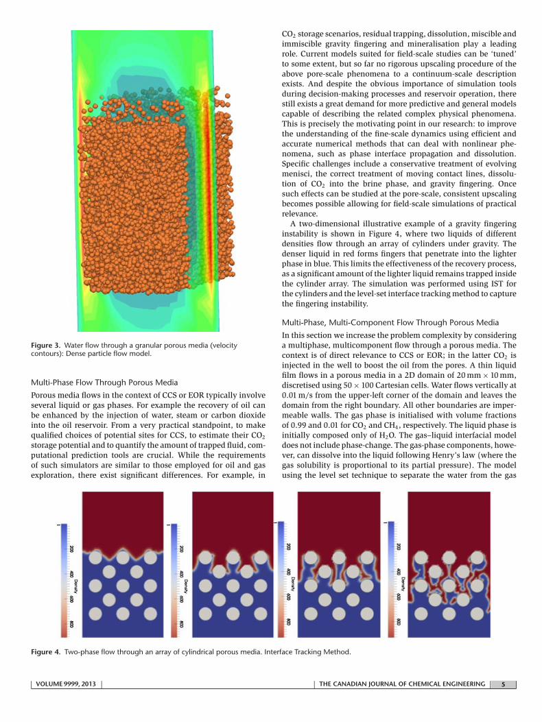
Figure 3. Water flow through a granular porous media (velocitycontours): Dense particle flow model.
Multi-Phase Flow Through Porous Media
Porous media flows in the context of CCS or EOR typically involveseveral liquid or gas phases. For example the recovery of oil canbe enhanced by the injection of water, steam or carbon dioxideinto the oil reservoir. From a very practical standpoint, to makequalified choices of potential sites for CCS, to estimate their CO2
storage potential and to quantify the amount of trapped fluid, com-putational prediction tools are crucial. While the requirementsof such simulators are similar to those employed for oil and gasexploration, there exist significant differences. For example, in
CO2 storage scenarios, residual trapping, dissolution, miscible andimmiscible gravity fingering and mineralisation play a leadingrole. Current models suited for field-scale studies can be ‘tuned’to some extent, but so far no rigorous upscaling procedure of theabove pore-scale phenomena to a continuum-scale descriptionexists. And despite the obvious importance of simulation toolsduring decision-making processes and reservoir operation, therestill exists a great demand for more predictive and general modelscapable of describing the related complex physical phenomena.This is precisely the motivating point in our research: to improvethe understanding of the fine-scale dynamics using efficient andaccurate numerical methods that can deal with nonlinear phe-nomena, such as phase interface propagation and dissolution.Specific challenges include a conservative treatment of evolvingmenisci, the correct treatment of moving contact lines, dissolu-tion of CO2 into the brine phase, and gravity fingering. Oncesuch effects can be studied at the pore-scale, consistent upscalingbecomes possible allowing for field-scale simulations of practicalrelevance.
A two-dimensional illustrative example of a gravity fingeringinstability is shown in Figure 4, where two liquids of differentdensities flow through an array of cylinders under gravity. Thedenser liquid in red forms fingers that penetrate into the lighterphase in blue. This limits the effectiveness of the recovery process,as a significant amount of the lighter liquid remains trapped insidethe cylinder array. The simulation was performed using IST forthe cylinders and the level-set interface tracking method to capturethe fingering instability.
Multi-Phase, Multi-Component Flow Through Porous Media
In this section we increase the problem complexity by consideringa multiphase, multicomponent flow through a porous media. Thecontext is of direct relevance to CCS or EOR; in the latter CO2 isinjected in the well to boost the oil from the pores. A thin liquidfilm flows in a porous media in a 2D domain of 20 mm × 10 mm,discretised using 50 × 100 Cartesian cells. Water flows vertically at0.01 m/s from the upper-left corner of the domain and leaves thedomain from the right boundary. All other boundaries are imper-meable walls. The gas phase is initialised with volume fractionsof 0.99 and 0.01 for CO2 and CH4, respectively. The liquid phase isinitially composed only of H2O. The gas–liquid interfacial modeldoes not include phase-change. The gas-phase components, howe-ver, can dissolve into the liquid following Henry’s law (where thegas solubility is proportional to its partial pressure). The modelusing the level set technique to separate the water from the gas
Figure 4. Two-phase flow through an array of cylindrical porous media. Interface Tracking Method.
| VOLUME 9999, 2013 | | THE CANADIAN JOURNAL OF CHEMICAL ENGINEERING | 5 |

Figure 5. Multiphase multicomponent flow across a porous medium.
phases; the latter are treated separately by solving a transportequation for each of the species. The porous media is representedby an ad hoc structure constituted by random cubical obstacles;it could have been similar to the array of cylinders presentedprevious to this section.
Initially the water front moves with gravity effects downwardbefore penetrating the structure (Figure 5); it is perhaps impor-tant to note that in the level set approach used here, a triple-linemodel is included to account for wetting of the front on the rockpores. The model is based on the triple force decomposition ofYoung’s; see Friess and Lakehal[14] for more details. It is remar-kable to note that the chemical reaction between the two gaseousspecies operates from the water front inward to the gas mixturephase. Note that there is no mass diffusion allowed between thegaseous phases and the liquid. CO2 phase is consumed slowly asthe water front evolves within the structure. While this exampleis an idealised configuration, the results suggest that this type ofsimulations could now be employed to predict real CCS problems.
DESTRATIFICATION IN LNG TANKS
Storage tanks for Liquefied Natural Gas (LNG) are usually filledwith LNG of different densities. Stratification may occasionallylead to rollover and rapid tank pressure rise, which could be harm-ful to the filling operation and may break the flow assurance. TheLNG stations should be properly designed to prevent the ventingof natural gas from LNG tanks, which can cause evaporative gasemissions and result in fluctuations of fuel flow and changes ofits composition. LNG tanks commonly have two types of fillingnozzles, top and bottom. Choice of filling point depends on whe-ther the cargo LNG is more or less dense than the LNG already inthe tank (the heel). Basically, bottom filling of lighter LNG and topfilling of heavier LNG are recommended. Stratification depends onthe nozzle, the initial density difference, the depth of the heel andthe filling rate. Also, the injection of a lighter LNG at the bottomof a stratified storage tank leads to large-scale motion inside thetank, which affects the rate of mixing and time for stratification.
Figure 6. Volume fraction contour of lighter LNG during reception intostorage tank.
The problem was borrowed from the work of Koyama[15] whoused the two-fluid, six-equation model. Instead in TransAT wehave tested for the same problem using two alternative strategiesexplained above: the N-phase mixture model in which the inter-phase slip is algebraically prescribed, and the level set techniqueproviding a clear distinction of the front. Turbulence was in allcases modelled using a simple URANS approach modified to copewith buoyancy effects. Right at the injection and depending onthe initial temperature difference and injection rate, large scalestructures are observed with size up to half of the tank. Theseenergetic events tend to mix very strongly the phases, causingdelays in the final desired stratification of the tank. These large-scale motions could be seen from the velocity field depicted inFigure 6. This effectively mixes the LNGs of different densitiesand de-stratifies the storage tank. The time evolution of the LNGdensity profile is shown in Figure 7. The CFD results agree withexperimental data taken from Koyama.[15] When use was made ofthe N-phase model, the results were not as good.
Figure 7. Mixed LNG storage—Comparison between calculated andmeasured density profile.
| 6 | THE CANADIAN JOURNAL OF CHEMICAL ENGINEERING | | VOLUME 9999, 2013 |

Figure 8. Cross-section of wells employing gas lift. Courtesy:Schlumberger.
GAS LIFT
In the gas-lift technique, gas is injected at the bottom of a pro-duction pipe (through which oil and water are flowing) in orderto reduce the gravitational pressure drop in the well. This resultsin an increase of the oil flow rate in the pipe. In practice, gas isinjected from valves attached to the pipe wall, which generateslarge bubbles. Previous work[16] with water and air indicates thatthe gas-lift efficiency can be improved by injecting small bubbles.The gravitational pressure drop is then reduced because: (i) therise velocity of small bubbles is lower, and hence the residencetime and void fraction in the pipe are higher, (ii) small bubbles aremore evenly distributed over the cross-section of the pipe, whichincreases the gas void fraction and (iii) small bubbles postponethe transition from bubbly flow to slug flow, which is an undesi-rable operating condition for gas-lift. A schematic of the gas-lifttechnique is shown in Figure 8.
We have conducted a preliminary feasibility study, using thelevel-set technique to track the gas bubbles injected at the bottomof a vertical riser filed with water; no oil is considered. The simu-lation was performed under 2D axisymmetric conditions. The gasis injected at the bottom (see Figure 9) at different flow rates,and the pressure drop is calculated for different values of the gassuperficial velocity at the injection nozzle. The form of the nozzleis also idealised, although we have ensured that the gas flow isinjected downward. The results shown in Figure 9 for variablegas flow rates indicate how the model is capable of predictingbubbles of different sizes rising in the pipe at different speedsand taking specific zigzag paths. Interestingly, with the level setmethod there is no need to adjust the drag or lift coefficient, thelatter is known to heavily affect the motion of the bubbles, driftingthem towards the wall or towards the core flow, depending on thesize. These results should of course remain qualitative only. Moreimportantly from a global viewpoint, the CFD prediction is in linewith the experimental results, in that injecting even a relativelysmall quantity of gas tends to significantly reduce the pressuredrop in the riser, as shown in Figure 10.
MULTIPHASE FLOW IN VERTICAL PIPES
Motivations
As stated in Introduction Section, gas–liquid flow in pipes is ofgreat practical importance in petroleum engineering, in particu-lar for separation and transportation. Mixtures of gas and liquids(light and heavy components of oil, solid particles, hydrates, wax,condensate and/or water) are produced and transported togetherunder various topologies (e.g. bubbly, slug, annular, mist) (Figure11). In addition, the relative volumetric fraction of the phasescan change along the pipes either because of heat addition, heatexchange between the phases or flashing due to depressurisa-tion. In vertical pipe flows, for example risers, the flow regimeidentification (up to three main phases, plus when possible sandand hydrates) is critical for the success of drilling and produc-tion. The main task in modelling multiphase pipeline flows is theidentification of the flow-regime map.
Current predictive tools for multiphase flow and heat transferin pipes are based on the two-fluid, six-equation model, in which
Figure 9. Gas injection in a vertical pipe for superficial velocities of 0.2, 0.5 and 1 m/s at the injection nozzle. Black contours show the gas bubbles.
| VOLUME 9999, 2013 | | THE CANADIAN JOURNAL OF CHEMICAL ENGINEERING | 7 |

Figure 10. Pressure drop for increasing superficial gas velocity at theinjection nozzle.
the conservation equations are solved for each phase. In the oiland gas industry this model is reduced to 1D, and is commonlyreferred to as the ‘Mechanistic Model’. Solution of the Mecha-nistic Model equations requires specification of closure relationsfor flow characteristics such as local velocities, wall shear stress,liquid holdups, etc. These closure relations carry the largest uncer-tainties in the model and are typically empirical, making use ofover-simplified assumptions; in particular, the geometry of thevapour/liquid interface is always idealised, for example sphericalor bullet-shaped bubbles, smooth or sinusoidal wavy liquid films,spherical or elliptic droplets. The physical reality of the situation is
Figure 11. Flow regime variation in a vertical pipe with gas superficialvelocity (with permission[34]).
much more complex, as shown in Figure 11, displaying the variousflow regimes encountered in ‘controlled’ laboratory experiments.Furthermore, the closure relationships are often developed fromlow pressure, small diameter pipe (typically 25–75 mm) datausing synthetic oil and air, which does not simulate actual fieldconditions, making upscaling to predictive codes highly uncer-tain. All these uncertainties in the closure relations reflect onthe overall accuracy of the predicted figure of merit, for examplepressure drop. For example, the codes adopting the MechanisticModel and used by the oil industry could predict the pressuredrop in a vertical riser with an error of more than 60.%[6] Theclosure relations are flow regime dependent and it is well knownthat flow regimes in large pipes (300 mm diameter, like deep-seariser pipes) differ significantly from those in smaller pipes. Forexample, slug flow is replaced by cap flow in large pipes because oflarge-bubbles instabilities. The complexity increases when morethan two phases evolve in the pipe, for example gas, water andoil. In this case the flow regime map is expected to feature a broa-der domain for churn and annular flow, the topology of whichremains difficult and expensive to investigate experimentally.
In horizontal pipe flows, the main open issue requiring bet-ter understanding is the transition from stratified flow to slugflow.[17] Slug flow is a commonly observed pattern in horizon-tal and low upslope gas liquid flows. The regime is associatedwith large coherent disturbances, due to intermittent appearanceof aerated liquid parcels filling the pipe cross-section. As theseaerated liquid parcels travel downstream the pipe, large pres-sure fluctuations and variations in flow rates could occur, whichcould affect process and separation equipment. Our recent CMFDresults[18] of flow transition in horizontal pipes has clearly shownthe importance of relying on advanced 3D simulation techniques,and has shed light on subtle mechanisms in association withsurface deformation, sealing and slug displacement.
Air–Water Flow in a Vertical Pipe
Measurements of a mixture of gas–water flowing in a vertical pipeof 6.7 cm diameter and 6 m length with various superficial airand water velocities were conducted at the Chemical EngineeringLaboratory of the University of Nottingham, UK.[19] Liquid andair were mixed at the bottom of the pipe by a special mixingdevice. The liquid enters the mixing chamber from one side andflows around a perforated cylinder; air is injected through a largenumber of 3 mm diameter orifices, thus, gas and liquid could bewell mixed at the test section entry. Inlet volumetric flow rates ofliquid and air were determined by a set of rota-meters. Gas voidfractions were measured at a height of 5 m using a wire-meshsensor.
The bubbly flow cases (1st two panels of Figure 11) weresimulated and published in another contribution,[18] and arethus not discussed here. Two cases were reproduced numericallyusing the code TransAT: In Case 1, the gas superficial velo-city is JG = 0.57 m/s, for a comparable liquid superficial velocity:JL = 0.25 m/s. According to Szalinski et al., this is a flow featuringa clear Taylor bubble, corresponding to the 7th panel of Figure 11.Case 1 is an intermittent slug flow with by a cloud of smallerbubbles trapped in the wake of the large cell. In Case 2, the gasand liquid superficial velocities are JG = 45 m/s and JL = 10 m/s,respectively, which corresponds to the annular flow regime, as inthe rightmost panel of the figure.
3D Slug Flow Simulation Results
Case 1 includes the formation of air slugs or Taylor bubbles tra-velling upward along the pipe, which makes it more complicated
| 8 | THE CANADIAN JOURNAL OF CHEMICAL ENGINEERING | | VOLUME 9999, 2013 |

Figure 12. 3D LEIS simulation (Level Set + LES) of a transition to slugflow.
to model because of the simultaneous presence of large and smallbubble structures trapped in the wake, and associated unsteady‘meandering’ of the flow and more active turbulence generateddue to the interaction of the phases, and between the aeratedstructures of different size. The chosen pipe length is only 3.1 mto ensure sufficient grid resolution and reasonable CPU time. TheAlgebraic slip model has been used although it is well known thatthis approach applies only for flows laden with small bubbles ofsizes comparable to the grid size. The modelling of the drift velo-city is another issue, since it requires the average bubble radius.Although we are aware that this class of models cannot be appliedfor slug flows, we have used it nonetheless, assuming a bubbleradius of 3.0 mm (otherwise the model crashes).
The 3D simulation was performed on a HPC supercomputerwith 128 Processors. Level set has been combined with full LESfor turbulence (the combination is known as LEIS [3]), using theWALE subgrid-scale model.[20] The grid consists in 3 million cells.The Immersed Surface Technique (IST) was employed, in that aCAD representing the pipe has been simply immersed in a Car-tesian grid. Near-interface treatment of turbulence follows themodel proposed by Liovic and Lakehal[21] and Reboux et al.[22]
High-order schemes were employed, up to 3rd-order RK for timemarching, and 2nd-order central scheme for convection fluxes;the Quick scheme was used for solving the level set equation.The time-step varies in time (bounded by convection, diffusionand surface tension CFL-like limiters ∼0.4–0.7) depending on thetopology of the flow, decreasing when small bubbles appear, downto 10−5 s sometimes. Understandably this first attempt has beenmade possible thanks to the available HPC resources only. Thesimulation of 6 s reproducing four slugs required 22 H on theHPC supercomputer.
Figure 12 clearly shows that the LEIS approach provides a richpicture of the flow as might be in reality and is qualitatively muchcloser to the experiment: cf. 4th panel of Figure 11. Slugs of dif-ferent sizes and elongations form naturally without triggering
their onset, occupying the entire pipe and travel upwards. Swarmsof bubbles are also generated in the wake, populating the area bet-ween the Taylor bubbles. Our videos show actually that the bubblecloud is primarily a result of fragmentation of the Taylor bubblewake due to strong interfacial shear dominating surface tension.Despite the qualitative picture, this grid is not sufficient to resolvethe cloud of bubbles as depicted in the experimental images. Fur-thermore, because of the grid resolution, grid-size bubbles formedtend to disappear. Also, time averaged profiles could not be gene-rated, because steady-state ergodic conditions require averagingover at least 10 Taylor bubbles travelling along the pipe.
3D Annular Flow Simulation Results
For the annular flow regime (Case 2), the dimensions of the pipewere reduced to 3 cm × 100 cm. With a grid of 800 000 points, thesimulation required 32 h to perform 20 000 iterations on a HPCcluster, using 128 cores. The numerical method and parameterswere the same as for the slug flow simulation discussed above.The resulting time step was approximately 6 × 10⁻⁶ s. Here, too,the level set approach was used in connection with LES for turbu-lence; basically the same model setup as in the previous slug flow.In reality the film thickness is quite small compared to the valueset in this case, otherwise a much larger grid would be requiredto resolve the film.
Density contours marking the interface and cross-flow veloci-ties vectors of the air–water pipe flow are shown in Figure 13. Thecoherent structures of the water film can be seen in both stream-wise and spanwise directions. Only in a few locations we couldobserve water parcels migrating to the core flow. This is a remar-kable result that has been so far with the realm of speculation only.The evolution of the water film thickness on the walls is reportedin Figure 13 at different cross-sections, indicating that the flow isnot yet fully developed and the comparison with the data of velo-city and density profiles would require a longer pipe. Althoughpresented as a proof-of-concept only, these LEIS results are veryencouraging and demonstrate TransAT’s capabilities for simula-ting multiphase vertical pipe flows. Such an approach provides anovel versatile method for exploring/explaining riser flows.
Figure 14 shows three cross-flow locations of the pipe, featuringthe liquid film deformation. It is interesting to note that there isa certain radial coherence of the events. Occasionally we couldobserve detached droplets migrating to the core flow.
Figure 15 depicts the evolution of the liquid film thickness inthe annular flow regime taken at z = 70, 80 and 90 cm. The plot-ted values are normalised by the initial liquid film height. Oneobserves how intense the deformation of the interface could be,with fluctuations around the mean reaching ∼400%. The fre-quency of the coherent waves could be extracted from the resultsbelow, indicating that it may change with time by up to one order,that is 125 < f < 275 Hz.
SUBSEA HYDRATE FORMATION AND PLUGGING
Background
Subsea hydrate formation may cause blockages in oil productionlines, and as such it remains today one of the main concerns todeepwater field developments. The present strategy of operatorsis commonly focused on the deployment of prevention methodsthat aim at producing outside the hydrate domain. This can mainlybe achieved via pipeline insulation (for oil systems) or chemicalinjection (for gas systems). Another strategy is to produce insidethe hydrate domain and transport the hydrate phase as slurry of
| VOLUME 9999, 2013 | | THE CANADIAN JOURNAL OF CHEMICAL ENGINEERING | 9 |

Figure 13. 3D LEIS in the annular flow regime. Snapshots of the flow shown at three different times.
hydrate particles dispersed in the oil phase, which led to develop-ments of Anti-Agglomerant. Even so, injection of such chemicalsremains marginal. Similarly, natural surfactants (e.g. asphaltenes,resins, etc.) present in most of black oils were also consideredas potential agents enabling hydrates to be transported as slurry.Operators envisage taking advantage of such surfactant propertiesto ensure restarting after a long shutdown.[23]
Various studies report on crude oils and hydrate control.[24,25]
Most of these studies show results on plugging or non-pluggingoccurrence in laboratory facilities though under flow conditionsinside the hydrate domain.[26,27] In terms of simulation, 1D modelsfor hydrate-plug formation in flowlines are available, and havebeen successfully applied for subsea tiebacks. Three-dimensionalfull CFD predictions are however rare in this area.
Improving the understanding of the flows occurring in risersand associated subsea oil production equipment is becomingimportant to respond to possible incidents such as the Macondoevent. The objective of resorting to detailed CFD is to improvethe realism and accuracy of predictions of the behaviour of multi-phase flows in risers and to improve the understanding of complexflow phenomena associated with deepsea hydrocarbon spills,including multiphase flow jet evolution, hydrate formation anddissolution, thermodynamics of hydrocarbon mixtures during fastpressure and temperature changes, and transient interaction ofplume constituents with the surrounding turbulence. The CMFD
code TransAT is one of the rare tools capable of predicting subseamultiphase hydrocarbon flows. The model is specifically dedi-cated to N-phase flow systems featuring complex fluid physics,including hydrate kinetics, formation and dissolution, deep-seathermodynamics, and very complex rheology. In addition, thecode is capable of predicting wall adhesion of the hydrates plug-ging on piping internals.
Hydrate Plugging of Subsea Equipment
One of the key issues in modelling hydrate plugging of flow-lines and equipments is to determine whether the hydrates stick(adhere) to the solid wall or not. In the former case, it is alsounclear which of the hydrates really do stick: the ones formedby methane phase change in contact with cold water, or thoseformed by the light components of oil? For the purpose, severalmodels have been developed and implemented in the code Tran-sAT, one of which is based on the stability principle of the hydratesin contact with the walls, combined with an advanced rheologymodel similar to Bingham’s model.[24] Prior to using the modelfor hydrate plugging of subsea caps, for example that employedby BP to cap the Macondo blow up, it was first employed to pre-dict the plugging of a vertical riser flow initially filled with oiland water and methane. The pipe dimensions and fluids flowrates are not important: it suffices to show that for the particularthermodynamics conditions selected, one can clearly see the
Figure 14. 3D LEIS in the annular flow regime. Snapshots of the pipe at three cross-flow locations.
| 10 | THE CANADIAN JOURNAL OF CHEMICAL ENGINEERING | | VOLUME 9999, 2013 |

Figure 15. Evolution of film thickness in annular flow regime at z = 70,80 and 90 cm.
nucleation of hydrates in the centre of the pipe developing upto a full plugging (Figure 16, left), as confirmed by the pressurecontours at corresponding times (Figure 16, right).
The hydrate model implemented within the N-phase mixturemodel was then used to predict the plugging in the canopyemployed by BP to collect the oil in the aftermath of the Macondoevent, for which experimental data of the canopy are availableonline (Figure 17, left). TransAT has been used to predict hydrate-induced plugging in the canopy taking hypothetical values only,without any specification or information from any source. 2Dsimulations were conducted first, using the N-phase model des-cribed earlier to deal with the various flow components. Themodel was used in combination with URANS for turbulence.The right panel of Figure 17 shows a snapshot of the flow fea-turing only oil (coloured) and water (blue), before activatingthe complete hydrate formation/adhesion/melting module. The
result (right panel) shows that the flow escapes partially from thecanopy. These first results have indicated that the jet flow featuresstrong unsteadiness and could only be well predicted using a timedependent approach; steady-state simulations are simply meanin-gless in this context. Since use of LES is prohibitive for similarproblems, we have extended the model to couple the N-phasewith hydrate module with V-LES, or Very Large Eddy Simulation,a strategy bridging LES with URANS that can be competitivelyadvantageous for very high Reynolds number flows.[18,28]
In a second step, use was made of the complete model nowunder V-LES to better capture flow unsteadiness. The results inFigure 18 suggest that the stability model employed in connec-tion with Palermo’s rheology model renders well the adherenceof the hydrates on the canopy internals, leading to a blockage ofthe flowlines that evacuate the oil via the riser (left column). Thefigures show the sequence beyond blockage, when oil starts esca-ping from the canopy. To try and prevent blockage, it was proposedto inject methanol from various small nozzles inside the canopy(not shown)—the effect of methanol is to locally lower the criticaltemperature of hydrate formation. In the presented case, althoughsome hydrates still adhere to the walls, the riser does not get blo-cked and almost no oil escapes the canopy (Figure 18, secondrow). Clearly, detailed CMFD provides an invaluable predictiontool for this problem. For more realistic flow conditions at theriser’s exit, however, this 3D simulation should be coupled witha 1D code to simulate the entire process: from oil collection nearthe source to its transport to the surface.
PARTICULATE FLOWS
Background
Particle-laden flows are of great practical importance in oil and gasengineering. The formation and accumulation of black powderin pipelines, for example, may be very harmful for hydrocarbontransportation installations and engineering studies are heavilyinvesting in computer-based predictive strategies to anticipatehypothetical black-powder slug formation and develop fast andefficient removal techniques to operate in time.[29,30] Similarly,promising oil extraction techniques such as hydraulic fracturinginvolve transporting a proppant, such as sand, into rock fracturesto keep them open and facilitate oil flow.[31] Because of the stronginteractions between the fluid carrier phase and the solid particles,advanced numerical methods are often needed for this class of
Figure 16. Hydrate formation and corresponding pressure in the pipe, at different times.
| VOLUME 9999, 2013 | | THE CANADIAN JOURNAL OF CHEMICAL ENGINEERING | 11 |

Figure 17. BP canopy used to resume oil spill in Macondo well. Flow simulated with TransAT (oil and water only). Only a portion of the riser isconsidered.
flows: Lagrangian particle tracking including four-way couplinginstead of average Euler–Euler formulations, Large-Eddy Simula-tion (LES) instead of RANS, and transient rather than steady-statesimulations.
Single-Phase Dense Particle-Laden Flows
To validate TransAT’s fluid/particle interaction models, simula-tions were performed for one experimental condition (Narayananand Janssen, 2009) of gas flow through a 6-inch horizontal pipe
at a system pressure of 10 bars and gas temperature of 20◦C.An initial mass of 200 g of particles (with sizes in the range200–400 �m) lies at the bottom of the pipe. The four-way couplingmodel (Equations 17 and 19) for dense-particle simulations wasused. Turbulence was resolved using the V-LES method. Consis-tently with what was observed experimentally, the particles aredragged along by the flow but remain near the bottom of the pipe.The critical velocity (defined here as the gas velocity needed totransport 10% of the initially injected dust mass over the 6.1 m
Figure 18. BP canopy used to resume oil spill in Macondo well (oil, water, methane and hydrates). First row: without methanol. Second row: withmethanol.
| 12 | THE CANADIAN JOURNAL OF CHEMICAL ENGINEERING | | VOLUME 9999, 2013 |

Figure 19. Black powder re-entrainment in pipe flow. Snapshots areshown at different times. Particles are coloured by size.
length of the pipe) was found to be within 10% of the 3 m/sfound experimentally.[32] Under different conditions, with largerparticles, the turbulence within the carrier phase simulated by V-LES generated sufficient flow unsteadiness to lift up the particlesand move the deposited bed through re-entrainment in the core ofthe flow. Snapshots of the flow are shown in Figure 19, depictingparticle concentration in the bed (coloured by their size) and theflow developed through the interaction with the carrier phase.
The distribution of particles in the vertical direction was vali-dated against experimental results from Laın and Sommerfeld.[33]
The setup is a 2D channel of height 3.5 cm and length 6 m. Theparticles have a diameter of 130 �m and a density of 2450 kg/m3.The void fraction of the inflow fluid is set to 0.00093, with a meaninflow velocity of 20 m/s in the x-direction and a standard devia-tion of 1.6 m/s in x and y directions. The initial angular velocityof the particles is set to 1000 s−1. A grid size of 125 × 34 was used.The simulations were run using the two-way coupling model anda Langevin forcing to account for the effects of turbulence onthe particles. The wall collision model for particles from Laın andSommerfeld[33] was used to take wall roughness into account. Theresults in Figure 20 show excellent agreement between the fluidand particle velocity profiles measured experimentally and thatsimulated by TransAT. The simulation also accurately predicts thepressure drop along the channel (the results are shown for a wallroughness gradient of 1.5).
CONCLUSIONS
The progress made in predicting multi-phase flows with high fide-lity in the context of oil and gas problems has been reported.Complex multi-phase, oil and gas problems are shown to be withinreach of modern 2D and 3D CMFD techniques implemented inthe code TransAT. The examples were presented to demonstratethe capabilities of CMFD simulations in general and TransAT inparticular. Deeper insight into each individual problem wouldof course require a dedicated study to exploit the rich database
Figure 20. Mean air and particle velocity profiles (left). Mean pressuredrop at streamwise locations L (right).
generated in the simulations. Most of the models can be fur-ther refined and adapted for various scenarios. It is true thatvarious limitations and roadblocks need to be alleviated beforesuch CMFD techniques could be efficiently used and provide areal added value to the various processes, as is the case today with1D codes like OLGA, LEDAFLOW, etc. Present effort is dedicatedto the coupling of TransAT with 1D codes to cope with specificproblems requiring more than one single strategy.
REFERENCES
[1] G. F. Hewitt, Nucl. Eng. Des. 2005, 235, 1303.[2] S. Nesic, Corros. Sci. 2007. 49, 4308.[3] D. Lakehal, Nucl. Eng. Des. 2010, 240, 2096.[4] A. Ansari, N. Sylvester, C. Sarica, O. Shoham, J. A. Brill,
SPE J. 1994, 152, 143.[5] J. Xiao, O. Shoham, J.A. Brill, Proc. SPE ATCE, New
Orleans, LA, 23–26 September 1990.[6] R. Belt, B. Djoric, S. Kalali, E. Duret and D. Larrey, Proc.
Multiphas. Flow BHR, Cannes 2011.[7] M. Manninen, V. Taivassalo, VTT Pubs. 1996, 288, 67.[8] D. Lakehal, M. Meier, M. Fulgosi, Int. J. Heat Fluid Flow
2002, 23, 242.[9] M. Sussman, P. Smereka, S. Osher, J. Comput. Phys 1994,
114, 146.[10] C. Narayanan, D. Lakehal, Phys. Fluids 2006, 18, 093302.
| VOLUME 9999, 2013 | | THE CANADIAN JOURNAL OF CHEMICAL ENGINEERING | 13 |

[11] D. Gidaspow, Appl. Mech. Rev. 1986, 39, 1.[12] S. E. Harris, D. G. Crighton, J. Fluid Mech. 1994, 266, 243[13] D. M. Snider, J. Comput. Phys. 2001, 170, 523.[14] H. Friess, D. Lakehal, 3rd ICHMT symposium on advances
in computational heat transfer, vol 2, 2004.[15] K. Koyama, Syst. Modell. Simul. 2007, 2, 39.[16] S. Guet, G. Ooms, R. V. A. Oliemans, R. F. Mudde, AIChE J.
2003, 49, 2242.[17] P. Valluri, P. D. M. Spelt, C. J. Lawrence and G. F. Hewitt,
Int. J. Multiphas. Flow 2008, 34, 206.[18] D. Lakehal, M. Labois, C. Narayanan, Prog. Comput. Fluid
D. 2012, 12, 153.[19] L. Szalinski, L. A. Abdulkareem, M. J. Da Silva, S. Thiele,
D. Lucas, V. Hernandez Perez, U. Hampel, B. J. Azzopardi,Chem. Eng. Sci. 2010, 65, 3836.
[20] F. Nicoud, F. Ducros, Turbul. Combust. 1999, 62, 183.[21] P. Liovic, D. Lakehal, J. Comput. Phys. 2007, 222, 504.[22] S. Reboux, P. Sagaut D. Lakehal, Phys. Fluids 2006, 18,
105105.[23] N. F. Nygaard, 4th Int. Conf. on Multiphase Flow, Nice,
June 1989.[24] T. Palermo, R. Camargo, P. Maurel, J. L. Peytavy, 11th Int.
Conf. on Multiphase Flow, San Remo, 219, 2003.[25] R. Camargo, T. Palermo, Proc. of the 4th Int. Conf. on Gas
Hydrates, Yokohama Symposia, Yokohama, Japan, 19 May2002.
[26] P. Mills, J. Phys. Lett. 1989, 46, 301.[27] P. J. Riew, P. Ghallagher, D. M. Hughes, Dispersion of
subsea releases, HSE Books, Offshore Technology ReportOTH 95-465, 1995.
[28] M. Labois, D. Lakehal, Nucl. Eng. Des. 2011, 241, 2075.[29] N. A. Tsochatzidis, K. E. Maroulis, Oil Gas J. 2007, 105(10),
52.[30] J. Smart, J. Pipeline Eng. 2007, 6(1), 5.[31] J. Adachi, E. Siebrits, A. Peirce, J. Desroches, Int. J. Rock
Mech. Min. Sci. 2007, 44, 739.[32] C. Narayanan, M. Labois, D. Lakehal, 7th Int. Conf. on
Multiphase Flow, ICMF, 2010.[33] S. Laın, M. Sommerfeld, Powder Technol. 2008, 184, 76.[34] H.-M. Prasser, M. Beyer, H. Carl, D. Lucas, A. Schaffrath,
P. Schutz, F.-P. Weiß, J. Zschau, NURETH-10, Seoul 2003,152(1), 3.
Manuscript received September 28, 2012; revised manuscriptreceived January 15, 2013; accepted for publication January 15,2013.
| 14 | THE CANADIAN JOURNAL OF CHEMICAL ENGINEERING | | VOLUME 9999, 2013 |