Advances in Image Reconstruction Methods for Real-Time ...cds.iisc.ac.in/faculty/phani/Prakash_JIISc_2014.pdf · projection type image ... reconstruction algorithms for CT (voxel

Journal of the Indian Institute of Science

A Multidisciplinary Reviews Journal

ISSN: 0970-4140 Coden-JIISAD

© Indian Institute of Science

Journal of the Indian Institute of Science VOL 94:4 Oct.–Dec. 2014 journal.iisc.ernet.in

REV

IEW

S

†Supercomputer Education and Research Centre, Indian Institute of Science, Bangalore 560012, India.‡Institute of Neurology, Faculty of Brain Sciences, University College London, London, United Kingdom.*[email protected]

Advances in Image Reconstruction Methods for Real-Time Magnetic Resonance Thermometry

Jaya Prakash†, Nick Todd‡ and Phaneendra K. Yalavarthy†,*

Abstract | Magnetic Resonance Imaging (MRI) has been widely used in cancer treatment planning, which takes the advantage of high-resolution and high-contrast provided by it. The raw data collected in the MRI can also be used to obtain the temperature maps and has been explored for performing MR thermometry. This review article describes the methods that are used in performing MR thermometry, with an emphasis on recon-struction methods that are useful to obtain these temperature maps in real-time for large region of interest. This article also proposes a prior-image constrained reconstruction method for temperature reconstruction in MR thermometry, and a systematic comparison using ex-vivo tissue experi-ments with state of the art reconstruction method is presented.Keywords: HIFU, MRgHIFU, image reconstruction, temperature maps.

1 IntroductionMagnetic Resonance Imaging (MRI) provides invaluable visualization of anatomical structures and tumors for treatment planning.1 It has the capability of providing high-resolution images of soft tissues. In recent years, it has been shown that various MR parameters like T

1-weighted,

T2-weighted, proton density and Proton Resonant

Frequency (PRF) can be used to obtain tempera-ture maps distribution, which in turn could be used for thermotherapy. Note that T

1-weighted

and T2-weighted images are obtained due to the

variation in the temperature in soft tissue, as a result direct reconstruction of temperature maps could be performed. Thus MRI can be used to obtain temperature distribution during thermal treatment (thermotherapy).2

Many thermal therapies are prelevant, the most famous ones use focused ultrasound (FUS) or laser inducer interstitial thermotherapy (LITT).3 In LITT, a laser light produced by Nd:YAG laser hav-ing a wavelength of 1064 nm is used, the laser light is absorbed and converted to heat, which causes change in the optical properties of the tissue lead-ing to coagulation (thermal damage to proteins). This culminates in killing of cancerous tissues.4 It is a minimally invasive technique, where a fiber

optic cable carrying laser light is used with a diffu-sive tip to deposit energy precisely at the region of interest.3 As the fiber optic tip is quite small, it can only be used for treating small tumors,3 making it not ideal for treating large tumors. Usage of laser does not interfere with MR measurements, hence MRI can be used to obtain the k-space (Fourier) measurements while preforming thermotherapy using LITT. These recorded MRI measurements can be used in turn to obtain the temperature distribution at the region of interest. MR guided LITT (MRgLITT) was successfully used for treat-ment on various organs like brain, liver, bone and prostrate.5

Focused Ultrasound Surgery (FUS) or High- intensity Focused Ultrasound (HIFU) is an efficient noninvasive technique to treat patients having cancerous tumors.6,7 HIFU has been used exten-sively for treating breast tumors, uterine fibroids and brain lesions.8 One of the major advantage of HIFU is its ability to focus on the tumor site (highly localized), which is not possible with radi-ation therapy, hence making HIFU prone to lesser side effects. Note that both diagnostic ultrasound and therapeutic ultrasound uses sound waves in different frequency range to create the required effect (diagnose abnormality or treat tumor).

Jaya Prakash et al.

Journal of the Indian Institute of Science VOL 94:4 Oct.–Dec. 2014 journal.iisc.ernet.in388

The frequency of sound waves used in diagnostic ultrasound depends on the depth you need to image (region of interest). The typical frequency range used is 3–10 MHz ( 20 MHz for skin scan).9 While in therapeutic ultrasound, i.e. in HIFU, the frequency range used is in the order of 1–2 MHz.10 The most important aspect in HIFU treatment is that focusing of ultrasound beam at the tumor site leads to a temperature rise at the focal spot. This rise in temperature results in breakage of cell walls of tumor cells hence destroying the cells at the focal spot. The typical power output generated by diagnostic ultrasound is less than 5 mW/cm2, while it is greater than 100 mW/cm2 in therapeutic ultrasound.8,11

MR guided HIFU (MRgHIFU) and MRgLITT uses same MR physics to estimate the tempera-ture distribution. The basic idea in obtaining the temperature distribution from T

1-weighted and

T2-weighted MR images is that the relaxation times

used to obtain T1-weighted and T

2-weighted MR

images are affected by the temperature of the soft tissues.12 The change in relaxation time (used for T

1- and T

2-weighted images) is due to spin-lattice

relaxation present in the biological tissues.13,14 This relaxation occurs due to the dipole interaction of macromolecules and water molecules, which is observed mainly due to rotational and transla-tional motion.14,15 A rise in temperature will effect this motion leading to change in relaxation time, and hence changes will be reflected in the T

1- and

T2-weighted contrast.14,15 When Proton Resonance

Frequency (PRF) is the MR parameter, the rise in temperature at resonant frequency has a direct correlation to the change in phase of the recorded MR data.

The PRF contrast can also be used for esti-mating the temperature distribution.16 The MR signal frequency depends on the chemical envi-ronment of water hydrogen, increase in temper-ature changes this environment, which helps in measuring the temperature change.16 A hydro-gen atom contains protons which is shielded by electron, leading to a reduction in the reso-nant frequency.16,17 Hence in water molecule, the electron in the hydrogen atom is pulled by the bond between hydrogen and oxygen molecule resulting in increase in resonant frequency. An increase in temperature will twist, stretch and break the bond between hydrogen and oxygen atom.16,17 This leads to a modest increase in electron shielding of the hydrogen proton from the magnetic field, leading to a reduction in the net field observed by the proton and hence changes the overall resonant frequency. Using

PRF parameter, it can be shown that a phase change will directly correspond to temperature change.16–18

Obtaining high spatial-, temporal resolu-tion, and volume coverage at the region of inter-est (hotspot) is a challenge in MR temperature imaging.8 Temperature rise of several degrees of centigrade per second over a volume of few mil-limeter can be achieved by inducing a HIFU soni-fication.8 High spatial and temporal resolution for monitoring these rapid temperature changes is essential, currently a 2-D imaging sequence with just a few slices covering the hotspot is used. Tran-scranial MRgHIFU applications require optimal monitoring of three-dimensional (3D) tempera-ture maps with large volume coverage and high spatio-temporal resolution for accurate tracking of rapid heating at the focus and monitoring the heating at the near- and far-fields of the ultra-sound beam.19,20 The most critical part of obtain-ing the temperature map using MRgHIFU is in reconstructing the temperature maps in real-time. Real-time imaging can be possible by reducing the MR scan time and performing faster tempera-ture map reconstruction from the acquired MR data. To achieve real-time therapeutic imaging, advanced image reconstruction methods (based on compressive sensing) can be used, wherein the temperature maps estimation can be performed with lesser measurements, which inturn can lead to faster scan times.21

Current state of the art MR temperature map reconstruction techniques in MRgHIFU are using Model Predictive Filtering (MPF),22 Temporally Constrained Reconstruction (TCR),21 and paral-lel imaging with UNFOLD.23 Model predictive filtering requires prior knowledge about tissue acoustic and thermal properties for accurate esti-mation of temperature maps.22 This method uses Pennes bioheat equation as a model along with tis-sue acoustic properties to obtain the temperature distribution.22 Both MPF and parallel imaging with UNFOLD methods are not able to monitor the entire 3D volume of interest. Currently, TCR is the only established method that has the ability to provide large coverage 3D temperature meas-urements.24 TCR was able to achieve accurate tem-perature measurements with 1.5 1.5 3.0 mm spatial resolution, 1.7 s temporal resolution, and 288 162 78 mm volume coverage. A major lim-itation of TCR method was its inability to perform real-time temperature map reconstruction and was therefore limited to retrospective applications.

The usage of Graphics Processing Units (GPUs) was previously explored for performing back-


Journal of the Indian Institute of Science VOL 94:4 Oct.–Dec. 2014 journal.iisc.ernet.in 389

projection type image reconstruction in cone-beam CT (CBCT) in real-time.25 Iterative image reconstruction algorithms for CT (voxel driven), which requires scatter and gather operations are performed on GPU, similar kind of algorithms are proposed for PET and SPECT (line driven) and shown to provide good speedups.25 Similarly, GPU has also been used for acceleration of MRI image reconstruction, where the reconstruction is performed using a simple fast Fourier trans-form (FFT) from the MRI pulse sequence. These MRI image reconstructions are performed using optimized GPU implementation of FFT known as CUFFT provided by CUDA26 to advance MRI reconstruction schemes like parallel imaging combined with reconstruction based on conjugate gradient solver.27 GPU has been explored even in non-linear image reconstruction schemes like dif-fuse optical tomography,28 and bioluminescence tomography,29 which require matrix inversion operations, while fluorescence molecular tomog-raphy imaging scheme was parallelized using an open-source software called AGILE.30 The TCR algorithm (later explained elaborately in this review) implementation in GPU hardware can provide the required acceleration to perform real-time temperature map reconstruction.

The TCR algorithm gives reasonably accu-rate reconstruction with 2 to 6 times (17–50 %) reduction factor in the k-space (acquired) data, but it does not provide the high level of opti-mization that is required, especially if the desir-able compressed data is around 12 times (8%). Recent works in dynamic Computed Tomogra-phy (CT) has shown that better utility of prior image can result in better reconstruction with relatively less number of projection using a Prior Image Constrained Compressive Sensing (PICCS) image reconstruction.31,32 It is impor-tant to note that in CT high under-sampling will help in reduced dosage, while in MRI it helps in faster scan times (desirable in real-time temper-ature monitoring). Hence, usage of a variant of PICCS as Prior Image Constrained Image Recon-struction (PICIR) algorithm is seen to provide accurate reconstruction with less number of MR measurements.

This review elaborates various MR methods that can be used in providing temperature maps. Further, it introduces various existing state-of-art image reconstruction algorithms for MR thermometry and lists the advantages and dis-advantages of each one. Later part of the review explains the PICIR-type image reconstruction and real-time TCR (RT-TCR) based temperature map

reconstruction. The comparison with TCR algo-rithm with these methods is also provided through numerical and ex-vivo tissue experiments. Lastly, a brief write-up on future directions in MR tem-perature imaging is presented.

2 MR Temperature Imaging MethodsThis section reviews various ways of estimat-ing temperature distribution using different MR parameters like T

1-weighted, T

2-weighted, proton

density, diffusion coefficient and proton resonant frequency.

2.1 Temperature imaging using T1-weighted MR images

Noninvasive temperature monitoring can be performed as relaxation times are function of time.12 The longitudinal relaxation time refers to the T

1-weighted image. In the early 80’s Parker

et al. investigated the relation between temperature and longitudinal relaxation rates, given using the following relation14,15

1

11

2 20

2 2T

H

o o (1)

where is the gyromagnetic ratio, 0 the Larmor

frequency, H the local magnetic field induced by local magnetic moments, and

0 is the molecular

position correlation time. The molecular position correlation time is dependent on temperature via the following relationship,14,15

0constant

T

K

T (2)

where K can be considered as a constant (since the viscosity ( ) of water changes very less with temperature) and T represents the temperature. A linear behavior between the T

1 contrast and

temperature T was observed experimentally, and hence heuristically linear relationship was assumed.14,15

More recent works indicate that an increase in temperature leads to a change in the transla-tional and rotational motion.33 It is well known that the spin-lattice relaxation in biological tis-sues is observed as a result of bipolar interaction of macromolecules and water molecules which in turn depends on their translational and rotational motion. Hence, an increase in temperature is reflected in longitudinal relaxation (T

1) time. The

mathematical model that describes this variation is given as,14

Jaya Prakash et al.


T eE T

kTa

1

1( )

(3)

where Ea(T

1) is the activation energy of the relaxa-

tion time, k is the Boltzmann constant and T the absolute temperature.33 Using the above model, Bottomley et al. showed that T

1 contrast has a lin-

ear relationship with the temperature ( ),T T11

the same was proved using the dependence on relaxation time. The temperature depends linearly with the longitudinal relaxation time (T

1 con-

trast). But the contrast is also affected by the tissue type, given by39

T T T T m T Tref ref1 1( ) ( ) ( ) (4)

where Tref

is the reference temperature and m dT

dT1 , which is estimated empirically for vari-

ous tissues.34 Typical values of T1(T) is 1.4%/°C

for bovine muscle,35,36 0.97%/°C for fat,37 and 1–2%/°C for liver.38,39

The relation between the repetition time (TR), reference temperature (T

ref), flip angle

( ), m, and T1 contrast is given by temperature

sen sitivity ( )dSSdT as40

dS

SdT

m TR E

T T

( ( ))

( ) ( )( )

1 1

1

cos

E cos E Tref ref2 1 1

1 (5)

where S and E1 is given by39,40

S M sinE

cos E011

( )( )1 1

(6)

ETR

T T m T Tref ref1

1

exp( ) ( )

(7)

with M0 representing the equilibrium magnetiza-

tion. Note that the accuracy of MR temperature imaging depends on the accuracy of measuring and estimating the T

1-weighted contrast. Pres-

ence of lipids leads to artifacts in the T1-weighted

images, and hence cannot be used for MR ther-mometry; this can be overcome by using lipid suppression techniques.39 Obtaining accurate T

1-weighted images can be done using inversion

recovery methods, but these tend to be compu-tationally expensive. Hence T

1-weighted methods

are always used with multiple readout pulses (multiple slices are acquired simultaneously), making it more suitable for hyperthermia applica-tions.41 The above equations contain a coefficient (m, which is tissue dependent), typically this coef-ficient is not known for individual tissue type, and hence T

1-weighted measurements have a draw-

back of not providing quantitative temperature

maps during heating. Most T1-weighted temper-

ature map imaging are used in situations where rapid qualitative imaging is sufficient.42

2.2 Temperature imaging using T2-weighted MR images

The transversal relaxation time (T2) follows a sim-

ilar trend of a T1 relaxation time. The variation

of T1- and T

2-weighted contrast with exponential

time constant of autocorrelation function is given as43,44

1

5 1

4

1 212 2T

A c

L c

c

L c( ) ( ) (8)

1

103

5

1

2

1 222 2T

Ac

c

L c

c

L c( ) ( ) (9)

where A is a constant, c is approximately the aver-

age time required for a molecule to orient itself through solid angle of 1 degree, and

L is the

resonant frequency. The above equations can be rewritten as43

Tc

L c c1 T expE

kTa

2 01&; (10)

where o T

1ln(2). Hence, the temperature

depends linearly with both T1 and T

2-weighted

contrast until some condition (L c

1) holds, a decrease in temperature (from a very high tem-perature value) will result in a decrease in con-trast in this region. When

L c 1, then T

1

L c2 , leading to further decrease in temperature

(increase in the T1-contrast).43 Therefore, this

variation looks like a parabola having a minimum T

1 contrast at

L c 0.612, while a decrease in

temperature will result in increase in the value of

c. In case of T

2-weighted temperature imaging,

the T2-contrast increases with an increase in the

temperature until c T

2.43 But when

c T

2 con-

dition is not satisfied (at very low temperatures), T

2-contrast tends to remain a constant as this

situation resembles a solid body in the Nuclear Magnetic Resonance (NMR) spectrum, the change in T

2-contrast with temperature follows a sigmoi-

dal increase.45 A more elaborate discussion and derivation can be found in Freude’s lectures.43

Previous works have reported that T2 con-

trast increases with increase in temperature in aqueous solution. The T

2 contrast for the water

in the tissue is lower by a significant factor when compared to pure water. But as already discussed, a reduction in temperature will cause increase in T

2 signal, and an increase results in lower T

2

signal value,45 this observation has been used



for identifying irreversible tissue damage during thermal coagulation.

The relationship between the Signal to Noise Ration (SNR) and MR parameter is given as43

SNR B T I IT

Ttmeas

52

0

23

32 2

1

1( ) (11)

where N is the density of nuclei, B0 the external

magnetic field, T represents the absolute tempera-ture, I the nuclear spin, and t

meas the measurement

time. It can be observed that the SNR depends on the absolute temperature and the contrast (T

1- or

T2-relaxation times). The measurable power in

the Radio-Frequency (RF) coil is proportional to the resonant frequency (

L B

0), hence the

power of RF coils can be related to the SNR.43 The electronic noise is observed due to the frequency and the temperature which is given by T , this is also called as white noise.43 Note that the SNR definition is the same for both T

1- and

T2-weighted temperature imaging. T

2-weighted

temperature measurements in case adipose tissues are shown in Ref. 46. As with the T

1-weighted, the

temperature maps obtained through T2-weighted

are qualitative in nature, making them not ideal for MR thermometry.

2.3 Proton density based temperature imaging

MR signal in proton density weighted imaging is proportional to the number of spinning protons present in the region of interest. The is achieved by having a very long Repetition Time (TR) and Echo Time (TE) being very short, leading to mini-mal weighting of the relaxation time, thus obtain-ing a proton density contrast. The temperature can also be measured by measuring the proton density (PD). The proton density linearly depends on the equilibrium magnetization (M

0)47

PDh

MN I I B

kTB0

2 20

00 0

( )1

3 (12)

where N represents the spins per volume and h is the Planck’s constant. The susceptibility (

0) is

related to the absolute temperature (T) as,

01

T (13)

Hence, proton density can be used to esti-mate the temperature changes, for example the equilibrium magnetization change by a factor of 0.30 0.01%/°C between 37°C to 80°C.48

It is important to note that tracking a change of 0.3%/°C necessiates high SNR, typically a temperature sensitivity of 3°C can be achieved by having an SNR of 100.49 As already seen, the T

1-weight effects the temperature measurements,

to avoid the effect of T1 on temperature meas-

urement the repetition time of pulse sequence has to be increased in the order of 10 seconds. This restricts the usage of this method for retro-spective applications.50

Proton density (PD) MR parameter was used in many clinical scenarios, for instance PD was used for performing follow up scan after perform-ing MR guided therapy.51 Proton density based temperature imaging was used for measuring temperature changes in ex-vivo tissue samples like fat49 Variation of proton density with temperature was studied for adipose and muscle tissues.52 A decrease in PD was observed in the muscle tissue as temperature increased, but in adipose tis-sue the PD was found to increase initially as the temperature rose to 50°C, and then decrease as the temperature further increased.52

2.4 Diffusion based temperature imagingIn here, the MR parameter that is being used for measuring temperature is the diffusion coefficient via spin-echo sequence. The diffusion coefficient explains the thermal Brownian motion of the ensemble of molecules in the tissue, this motion occurs due to temperature variations in the tissue. The temperature is related to diffusion coefficient using the following relation53

D eE D

kTa ( )

(14)

where Ea(D) indicates the activation energy of

molecular diffusion of water. The variation of temperature with diffusion coefficient is given by

dD

DdT

E D

kTa( )

2 (15)

This MR parameter can estimate a tempera-ture change of about 2%/°C. The change in tem-perature can be derived as54

T T TkT

E D

D D

Drefref

a

ref

ref

2

( )( ) (16)

where D and Dref

indicates the value of diffusion coefficient at temperature T and T

ref (reference

temperature) respectively, this result assumes that T T

ref and that E

a is independent of T.

Jaya Prakash et al.


Note that the above equation shows that measuring temperature using diffusion coef-ficient does not depend on the magnetic field strength. This kind of measuring temperature was used for non-invasively measuring tempera-ture in-vivo.55 One of the major advantages of this method is its high temperature sensitivity, but this scheme suffers to provide real-time imaging as the acquisition time is very long (longer echo time required), and hence tends to be extremely sensitive to motion.55,56 Methods like single-shot Echo Planar Imaging (EPI)55 and line-scanning56 techniques have been used to overcome the limi-tations of long acquisition time and motion arti-facts. Another major disadvantage of this method is that temperature dependence on diffusion coef-ficient becomes non-linear when the tissue con-ditions change. The diffusion coefficient depends on the amount of water content, the movement of water is affected by proteins, membranes etc. Thermal heating may lead to protein coagula-tion, and hence avoid movement of water result-ing in different diffusion coefficient estimates. The lipid suppression in tissue containing fat has to be incorporated for using diffusion coefficient for estimating temperature maps, as variation in fat results in variation in diffusion coefficient with an increase in temperature.39 Previous works have used diffusion weighted MRI for early detec-tion of regional cerebral ischemia in cats,57 and later works have used EPI-diffusion coefficient weighted MR (lesser sensitive to motion) for non-invasive temperature monitoring in acryla-mide gel materials, and in-vivo in canine brain tissue.58

2.5 Proton resonance frequency based temperature imaging

Proton Resonant Frequency (PRF) was seen to be sensitive to temperature during the late 1960’s,13,59 and it was used for spectroscopy and then for MR temperature imaging. Water molecules contain two hydrogen atoms and an oxygen atom, the elec-tron in the hydrogen atom is pulled by the bond between hydrogen and oxygen molecule, resulting in increase in resonant frequency.16–18 This bond will twist, stretch and break with the increase in temperature.13,16,60 Increase in temperature will lead to electron shielding of the hydrogen atom from the magnetic field, thereby reducing the net field observed by the proton. This will change the overall resonant frequency, which can act as a sig-nal for MR temperature imaging.

The resonant frequency of the hydrogen atom is due to the presence of the local magnetic field. The field at the nucleus is given by16

B B B s Blocal s0 0 01( ) (17)

where Blocal

is the local magnetic field, B0 is the

applied magnetic field, and s is the shielding con-stant or screening constant (dependent on the chemical environment). The resonant frequency now becomes,

B B slocal 0 1( ) (18)

this shielding constant depends on the tempera-ture, hence proton resonant frequency can be used to estimate the temperature maps. The relation-ship between shielding constant s and tempera-ture T is given as,

s T T( ) (19)

where indicates some constant, hence the variation of temperature leads to linear varia-tion in shielding constant. Temperature map estimation using PRF shift can be done in two ways, spectroscopic imaging and phase mapping methods.

2.5.1 Spectroscopic imaging using PRF shift: Proton spectroscopic imaging used for tempera-ture imaging utilizes temperature induced water proton chemical shift. The frequency shift is com-puted using MR spectra, the shift is measured between water peak and reference peak (this peak remains constant with temperature), the model given in Eq. 18 is used to obtain the temperature map. Absolute temperature imaging is possible as the reference temperature does not get affected by field drift and motion during scan,61 hence abso-lute temperature imaging has been demonstrated in human brain.62

A spatial resolution of 3–4 mm was achieved by spectroscopic imaging, also the reconstruction of absolute temperature was performed within 1 minute. Various kinds of data acquisition meth-ods have been proposed for spectroscopic imaging, mainly used ones are Echo Planar Spectroscopic Imaging (EPSI), MR Spectroscopic Imaging (MRSI) and Line Scan Echo Planar Spectroscopic Imaging (LSEPSI).63 This method is used only for retrospective application due to its limitations to achieve high spatial and temporal resolution.63,64 A thorough study of the effect of MRSI with shimming, eddy currents, spatial localization and post-processing methods has been given by Drost et al.65 MRSI was used for measuring brain temperature, this helped in studying a variety of clinical conditions such as stroke, traumatic brain injury, and schizophrenia.66



2.5.2 Phase mapping using PRF shift: Phase mapping using PRF shift is a widely used imaging technique for obtaining the temperature maps. In this kind of temperature imaging, the phase image of the tissue before the heating is subtracted with the current on (after heating starts) to obtain the temperature distribution. As already described, the phase difference is proportional to the temper-ature-dependent PRF change and the echo time, the change in temperature is given as,16

TT T

B TE

( ) ( )0

0

(20)

where (T) indicates phase of the current image (data obtained after heating starts), (T

0) is the

phase before the heating has started, B0 is the mag-

netic field strength and echo time is indicated as TE.

The Gradient Echo (GRE) signal intensity decreases exponentially with increase in TE having a time constant T2

* . The signal to noise ratio depends on the echo time and can be derived to be39

SNR TEe

TET2 (21)

Here an optimal TE can be estimated to obtain a maximum SNR. Hence, differentiating the above equation with respect to TE and equating it to 0 results in obtaining optimal TE as TE T2 .63,67 A variety of effects like tissue type, electrical con-ductivity, external field shift and susceptibility which influence temperature measurements using proton resonant frequency shift is explain in greater detail by Rieke et al.39 This scheme is widely used in MRgHIFU for treating brain and breast tumors. The phase mapping using PRF shift is utilized in all discussed image reconstruction algorithms in this review.

3 Image Reconstruction in MR Thermometry

High spatial and temporal resolution of tem-perature maps is one of the key requirement in in MRgHIFU. High spatial resolution is required while treating organs like breast to avoid tempera-ture measurement errors due to partial volume effect.68 Increase in spatial resolution accommo-dates small and non-uniform shaped structures at the focal zone. Typical focal zone using HIFU is 13 mm 2 mm, the power deposited by using the ultrasound beams follows a Gaussian profile, and working with voxel size larger than 1–2 mm3 induces errors in temperature measurements due the averaging effects of the Gaussian.68

High temporal resolution is another essential aspect in MR thermometry, which enables mini-mizing the treatment time and better control of HIFU heating. Most important aspect is to know the end point of temperature heating (15–20°C above the body temperature), at which the tis-sue becomes necrosed.68 Not exceeding this target temperature is essential, as exceeding this temper-ature will lead to excessive heating in the near field of ultrasound beam.68 Excessive heating typically requires more time for cooling, hence an increase in total time of MRgHIFU therapy.68,69 Fast scan time is also essential as the temperature in the region of interest can rise at a rate of 3°C/sec and the thermal dose is known to double for every 1°C.68,70 Hence to obtain accurate temperature maps, the reconstruction algorithms should be able to provide high spatial and temporal resolu-tion with less number of measurements (k-space lines) alongwith imaging the entire Field of View (FOV) covering the full anatomy that is being treated.68 There are many reconstruction meth-ods available for performing temperature map reconstruction in MR thermometry, like solving the Pennes bioheat equation by Model Predictive Filtering (MPF), using parallel imaging with Una-liasing by Fourier-encoding the overlaps using the temporal dimension (UNFOLD), and Temporally Constrained Reconstruction (TCR). These are described in details in the subsequent sections.

3.1 Model predictive !ltering (MPF)MPF uses a thermal model (Pennes bioheat equa-tion), which is identified before the therapy begins. The temperature at next time points are predicted based on this temperature model, and this is used to create an estimate of the current k-space data.68 The temperature at the current time point is esti-mated using the updated k-space data and a com-bination of the estimated current k-space data and the acquired undersampled k-space data. The thermal model is based on Pennes bioheat equa-tion given by22

CT

tk T WC T T Qblood

2 ( ) (22)

where T is the temperature of the tissue, the tissue density, k the thermal conductivity of the tissue, C the specific heat of the tissue, Q the deposited power density, and W is the Pennes per-fusion parameter. Assuming that the specific heat of the blood and tissue is the same, the values for

and C can be considered as 1000 kg/m3 and 4186 J/kg/°C.68 The other parameter in the model like k, W, and Q are estimated before therapy using low

Jaya Prakash et al.


power continuous pulse and fully sampled k-space data during the heating and cooling phase. Note that the dimensionality of W and Q is same as that of the obtained MR data.

The volume is assumed to be homogeneous and thermal properties are assumed to be iso-tropic while estimating the parameters (W and Q). The parameter Q is estimated using pixel by pixel linear fit to the first two or three points of the temperature-time curves,22,68 this parameter estimation assumes that the perfusion and dif-fusion is negligible for small duration at the start of ultrasound heating. The scalar k (thermal con-ductivity) is estimated based on measured rate at which the Gaussian-shaped temperature profile of the sample spreads in the direction perpendicular to the ultrasound beam during cooling.22,68 Using this k, the W can be estimated numerically, at the beginning of cooling period, where Q is zero, via the relation22

WT

k

CT

T

t

1 2

(23)

The temperature at n 1 time frame can now be estimated using the Pennes bioheat equation,22

T Tk

CT

WT

u

CQ tn n n n

nrel1

2 . (24)

where Qrel

is the normalized power distribution, un

is the ultrasound power applied at nth time frame, and t is the time step. The spatial derivative ( 2) can be calculated numerically for each pixel. The first time frame of the acquired k-space data must be fully sampled.68 The next time frames can be sampled by a undersampling factor of S. The important steps in recursive model predictive fil-tering algorithm are22,68

1. With the current temperature estimate at time n as T

n, acquire the undersampled k-space data

at time frame n 1.2. Use the thermal model given by the bioheat

equation, estimate the new temperature Tn 1

at n 1 time frame using Eq. 24.

3. Create a complex image at time frame n 1 using the magnitude of image at nth time frame and calculate the phase (n 1) as, (n 1) (n)

B0

TE(Tn 1

Tn); 0.01ppm/°C.

4. This complex image is projected to k-space by taking a Fourier Transform.

5. The acquired undersampled data at time n 1, is filled with the corresponding predicted lines.

6. This updated k-space data is transformed to image space using inverse Fourier Trans-form and a new temperature distribution is estimated.

It can be seen that the above algorithm pro-vides a very good resolution, but has an inherent drawback of requiring to estimate many param-eters like , W, Q, k, and C.22 These parameters are generally tissue dependent, making this proc-ess computationally intensive task. But MPF based algorithm was shown to work well in presence of motion, due to inclusion of motion detection and correction steps into the algorithm.68 More details about MPF can be found in Ref. 22.

3.2 Parallel imaging with UNFOLDThis reconstruction technique assumes that ther-mal therapy takes place on much smaller Field of View (FOV) than the entire organ, thereby pro-viding faster temperature imaging. Fast imaging strategies like two-dimensional spatially-selec-tive RF (2DRF) excitation, unaliasing by Fourier encoding of the overlaps using the temporal dimension (UNFOLD), and parallel imaging are combined. The assumption is that 2DRF excita-tion approach is well-suited for temperature mon-itoring, as larger FOV is required to avoid aliasing, which is often substantially larger than the heated volume. The UNFOLD and parallel imaging tech-niques can be used to remove the aliasing artifacts introduced by 2DRF excitations, and enable use of shorter 2DRF pulse durations (thereby providing real-time imaging capability).

This algorithm assumes that the only a small part of the FOV is to be imaged and the Signal to Noise Ratio (SNR) is not a limiting factor.71 With these assumptions, the data is collected pertaining to this small FOV by acquiring fewer k-space lines, leading to faster acquisition time.71 This kind of data collection leads to aliasing artifacts from sig-nal outside the FOV, this could be overcome by using a 2DRF pulse to limit the excitation of the desired region of interest in the phase encoding direction.23 A RF field is a composition of mul-tiple sub pulses weighted with k-space weighting function, magnetic field gradient and the excita-tion profile. The excitation profile M(r) can be expressed as,23

M r i k S exp ir k dk( ) ( ) ( ) ( . )M W k0 (25)

where r and k are vectors. Here M0 indicates the

original longitudinal magnetization, S(k) is the



sampling function of the excitation k-space, W(k) is the weighting function, and k(t) is given as23

k t G dt

T( ) ( ) (26)

where G represents the gradient field. The weight-ing function W(k) is given as23

W k tB t

G tl( ( ))( )

| ( )| (27)

where Bl(t) is the RF field. The excitation profile can

be viewed as the Fourier transform of the product of k-space weighting function and k-space sam-pling function. In order to avoid aliasing artifacts, a RF pulse is required to create one excitation lobe within the FOV, but this leads to increase in mini-mum Repetition Time (TR) and hence scan time. On the other hand, short RF pulse leads to excita-tion profile becoming wider or the excitation pro-file repeating itself.23 To overcome this, one can use a shorter RF pulse and in the next step can include removal of the introduced aliasing artifacts using UNFOLD and parallel imaging methods.23

UNFOLD is a reconstruction scheme that takes into account the temporal evolution of the signal of every pixel of the image.72 The idea of UNFOLD technique is that in a dynamic imaging scenario, every pixel in an image has a correlated change observed in the temporal dimension.72,73 In the dynamic case, maximum signal content tends to appear in the DC component of the fre-quency domain of the temporal signal. UNFOLD algorithm tries to isolate the DC component from the aliased signal, thereby obtaining the unaliased version of the frequency domain data.72 Once the filtering operation is done, the image can be obtained by taking the inverse Fourier transform of the unaliased version of the signal.73

Parallel imaging involves using multi-ple receiver coils to collect the data in parallel, thereby reducing the scan time. The reconstruc-tion algorithms involving parallel imaging are SMASH (SiMultaneous Acquisition of Spatial Harmonics)74 and SENSE (Sensitivity Encoding),75 with SENSE being widely used due to its fast recon-struction time. In SENSE reconstruction, the dis-tance between the sampling position in k-space is increased while retaining the maximum k-value leading to reduction in scan time.75 This leads to aliasing due to reduction of sampling density, this aliased image is then used to create the full-FOV image from the set of intermediate images. This is achieved by estimating the signal contribution to

each pixel by its neighboring pixels.75 This kind of signal separation is possible due to the fact that in each single-coil image superposition occurs with different weights according to coil sensitivity.75 A sensitivity matrix is estimated based on this idea, and this is encoded into the reconstruction proce-dure. More details about the SENSE algorithm can be found in Preusmann et al.75

Above explained schemes can be combined in full/in part to obtain an accurate tempera-ture distribution for MR thermometry. Reduced FOV (rFOV) is imaged and corresponding data is obtained, this results in an aliased signal.23 The ali-ased signal can be corrected using parallel imag-ing and UNFOLD methods.23,76 Parallel imaging method can be used on aliased signals where there exist a large separation between the main lobe and the smaller side lobes.23 While UNFOLD can be used to separate regions that are present in close proximity, i.e. can be used to reduced the FWHM of the given Gaussian signal. Usage of these two schemes on the aliased signal results in an unali-ased signal.23 Later, temperature maps can be esti-mated using this unaliased signal.

3.3 Temporally Constrained Reconstruction (TCR)

Another widely used reconstruction method in MR thermometry is by applying a temporal regularization constraint. This method provides acceleration when k-space under sampling pat-tern is alternated in time. This induces some aliasing artifacts, but those are filtered out by usage of the penalty term (regularization). Tem-porally Constrained Reconstruction (TCR) is one of the currently available schemes, which has the capability to provide high spatial and tempo-ral resolution along with full three-dimensional coverage, which is essential for performing tem-perature imaging in MR thermometry. The only drawback of this scheme is that usage of alternat-ing k-space sampling patterns leads to eddy cur-rent distortion, and hence limits the acquisition design setup.

The temperature maps are obtained using a temporally constrained reconstruction (TCR), which is based on compressive sensing like approach enforcing the data fidelity and con-straining the rapid temporal change. This algo-rithm draws a parallel to the regularization theory for solving ill-posed inverse problems. The stand-ard discrete inverse Fourier transform reconstruc-tion from the full k-space data can be written as,21

d mF (28)

Jaya Prakash et al.


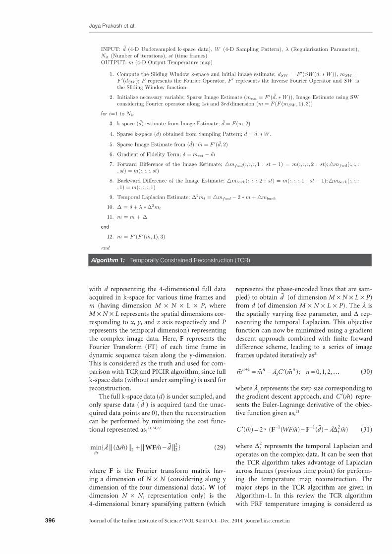
with d representing the 4-dimensional full data acquired in k-space for various time frames and m (having dimension M N L P, where M N L represents the spatial dimensions cor-responding to x, y, and z axis respectively and P represents the temporal dimension) representing the complex image data. Here, F represents the Fourier Transform (FT) of each time frame in dynamic sequence taken along the y-dimension. This is considered as the truth and used for com-parison with TCR and PICIR algorithm, since full k-space data (without under sampling) is used for reconstruction.

The full k-space data (d) is under sampled, and only sparse data ( d ) is acquired (and the unac-quired data points are 0), then the reconstruction can be performed by minimizing the cost func-tional represented as,21,24,77

min{ ||( )|| || || }m

m m d2 22WF (29)

where F is the Fourier transform matrix hav-ing a dimension of N N (considering along y dimension of the four dimensional data), W (of dimension N N, representation only) is the 4-dimensional binary sparsifying pattern (which

represents the phase-encoded lines that are sam-pled) to obtain d (of dimension M N L P) from d (of dimension M N L P). The is the spatially varying free parameter, and rep-resenting the temporal Laplacian. This objective function can now be minimized using a gradient descent approach combined with finite forward difference scheme, leading to a series of image frames updated iteratively as21

m m C m nn ns

n1 0 1 2( ); , , , (30)

where s represents the step size corresponding to

the gradient descent approach, and C m( ) repre-sents the Euler-Lagrange derivative of the objec-tive function given as,21

C m WFm d mt( ) * ( ( ) ( ) )2 1 1 2F F (31)

where t2 represents the temporal Laplacian and

operates on the complex data. It can be seen that the TCR algorithm takes advantage of Laplacian across frames (previous time point) for perform-ing the temperature map reconstruction. The major steps in the TCR algorithm are given in Algorithm-1. In this review the TCR algorithm with PRF temperature imaging is considered as

Algorithm 1: Temporally Constrained Reconstruction (TCR).



standard benchmark to compare the recently developed algorithms.

3.3.1 Advantages of temporally constrained reconstruction algorithm: TCR algorithm pro-vide high spatial resolution and temporal reso-lution while performing the temperature map reconstruction. TCR algorithm also has the ability to provide reconstruction for large Field of View (FOV). Even though Model Predictive Filtering (MPF) has the ability to provide high spatial and temporal resolution, MPF requires estimation of many parameters like W, Q, , k, and C (all these are tissue dependent). On the other hand, parallel imaging with UNFOLD has good spatial and temporal resolution, but has a limitation of not spanning larger Field of View (FOV), must be restricted to reduced FOV (rFOV) due to usage of 2DRF. Major drawbacks of TCR reconstruc-tion scheme is the eddy currents distortion and lacks the ability to perform real-time temperature imaging. Next section will explain the utility of graphics processing units (GPU) to eliminate the drawback of real-time imaging for TCR method. A real-time TCR (RT-TCR) algorithm that runs on the GPU, having a capability to provide high spatio-temporal resolution with large coverage along with real-time reconstruction (reconstruc-tion is faster than data collection time, making it ideal for MR thermometry). Since TCR is the only method to provide high spatial, temporal and vol-ume coverage, TCR is used for comparison with the PICIR algorithm (discussed later).

4 Real-Time Reconstruction in MR Thermometry

4.1 Real-Time Temporally Constrained Reconstruction (RT-TCR)

The original TCR algorithm can be used for per-forming dynamic three dimensional imaging. In here, the reconstructed image m can be obtained from k-space data, d , by iteratively minimizing the cost function:

m arg F d mmin 22

miN

t iW m|| ( ) || || ||22

(32)

where F indicates the Fourier Transform, W indicates which phase encoding lines have to be acquired, m is the image sequence estimate, and

is a regularization parameter. Real-time avail-ability of the temperature maps can be achieved using RT-TCR algorithm, for doing this the TCR algorithm is modified in two ways: the TCR code is implemented on Graphics Processing Units

(GPU) to reduce the computation time and the algorithm is applied to only a small section of the image matrix around the region of hotspot. Moreover, the estimates for the current tempera-ture map is obtained using only the current and past time frames.78

The original TCR algorithm is written in Matlab environment, hence this algorithm was rewritten on the GPU using open-source pack-ages namely CUFFT79 and CUBLAS80 provided by CUDA, and are wrapped to make them Mat-lab executable (mex) files, enabling running of the TCR algorithm on a GPU machine.78 The RT-TCR algorithm was implemented on a NVIDIA Quadro 6000 GPU machine having 448 cores and 6 GB memory. The data matrix is truncated in x- and z-directions in image space, such that only small ROI around hotspot is reconstructed using RT-TCR algorithm.78 The remaining region where temperature is static or changes very slowly is reconstructed using sliding window approach to enable faster reconstruction.78 The most recently acquired k-space data is added to the previous k-space frames in a sliding window fashion, hence enabling data truncation; this data is transformed to image space, truncating the x- and z-directions, and transforming back to k-space.78 Note that doing truncation in the y-direction is not possible as the undersampling is performed in the phase-encoding direction. This truncated, sliding win-dow k-space is used as the input for the RT-TCR algorithm.

The current time frame in the RT-TCR algo-rithm is reconstructed based on the current and past information, but also updates that time frame later as and when the future information becomes available.78 The location of the hotspot and the time frames at which the ultrasound is turned on/off is the only prior information given to the RT-TCR algorithm. To reconstruct the current time frame, t, the RT-TCR algorithm only uses frames [t P, t], where P is twice the data reduction fac-tor, more detailed illustration is given in Ref. 78. The performance of the RT-TCR algorithm can be seen as the original TCR algorithm to recon-struct a data set with 192 108 30 image matrix and all 77 time frames, it takes 236 seconds on a 12-core computer with Dual Intel Xeon Processor X5650, 2.66 GHz processing speed, and 64 GB of RAM.78 The truncated data having a matrix size of 10 108 13 using the 13 most recent time frame takes around 0.25 seconds using the RT-TCR GPU implementation on an NVIDIA Quadro 6000 with 448 cores. The data transfer from scanner to the computer having GPU card took 0.35 seconds, 0.02 seconds to do the necessary pre-processing

Jaya Prakash et al.


steps, and 0.10 seconds for the post-processing. Note that the total reconstruction time (0.72 sec-onds) is less than the data acquisition time for one undersampled time frame, thus removing the reconstruction bottleneck.78 The data reduc-tion along with GPU implementation produced a temperature map reconstruction in 0.72 seconds (including data transfer, running TCR algorithm on GPU, pre- and post-processing steps). Note that RT-TCR it is not faster than Fourier recon-struction, but is faster than one acquisition step, and therefore making it sufficient for the needed temperature feedback.78

The implementation of RT-TCR algorithm uses information from previous time frames to improve the image of the current time frame, but if the previous time frames are noisy then the noise will propagate making the estimate inac-curate.78 Another drawback of RT-TCR is with its inability to handle motion inside the FOV (which is also true for the TCR algorithm), but motion outside the FOV can be handled using the RT-TCR scheme.78 Despite these drawbacks, the advantage of RT-TCR lies with its ability to pro-vide increased volume coverage without sacrific-ing spatial or temporal resolution and real-time

Algorithm 2: Prior Image Constrained Image Reconstruction (PICIR).



reconstruction, making it suitable for monitoring temperature changes.

4.2 Prior Image Constrained Image Reconstruction (PICIR)

Another approach for achieving real-time recon-struction is by reducing the scan time, i.e. acquir-ing less number of measurements, without compromising the quality of the reconstructed temperature maps. At present, the TCR algorithm provides reasonably accurate reconstruction with 2–8 reduction factor in the data, higher reduction factor is desirable (resulting in faster scan time). TCR applied a temporal constrain to perform the image reconstruction, while in PICIR algorithm an extra term is added as a constraint involving the previous or the next time frame. The accuracy of the temperature map reconstruction can be improved by using the PICIR framework, where the minimization of the unconstrained variant is considered, namely31,32

min{ [ ||( )|| ( )||( )|| ]

|| || }m

prm m m

m dr

22

22

22

1

F (33)

with representing the non-negative regulariza-tion parameter and mpr being the prior informa-tion obtained as the previous or the next time frame. The prior image is defined as,

mm if i

P

m if iPpr

i

i

1

1

2

2

,

. (34)

where P represents the total number of time frames.

Here when the temperature is rising the pre-vious time frame should act as prior reference and for the falling temperatures the next time frame should act as prior reference. It is impor-tant to note that the first time point reconstruc-tion is performed by having fully sampled k-space data, the next time points have sampled version of the k-space data, which is similar to the TCR algorithm. The weight factor is represented by

( 1 indicates full weight for the prior and 0 indicates reconstruction performed using

the TCR approach).Solving of Eq. (33) can be done using a gra-

dient descent approach with finite forward differ-ence, leading to a series of image frames updated iteratively as

m m C m nn ns

n1 ( ); 0, 1, 2, (35)

where s represents the step size corresponding to

the gradient descent approach, and C m( ) repre-sents the Euler-Lagrange derivative of the objec-tive function given as,21

C( ) ( ( ) ( )(( ) ) ( ( )))

m m dm m mt pr

2 ** *

F WF F1 1

21 (36)

The major steps of PICIR algorithm for the 4-D temperature map reconstruction are indicated in Algorithm-2. The inclusion of this prior term into the minimization helps in performing the recon-struction with very less measurements compared to the standard TCR algorithm. It is important to note that in both the TCR and PICIR algorithms, the sliding window reconstruction is used as the initial image estimate (current TCR works in this fashion). The comparison of this scheme (PICIR algorithm) is performed using ex vivo pork mus-cle experiments, which will discussed in the next section.

5 Simulations and Results5.1 Simulation and experimentsThe PICIR method was evaluated using MRgHIFU data sets. The HIFU heating were performed in a Siemens TIM Trio MRI scanner (Siemens Medi-cal Solutions, Erlangen, Germany) using an MRI-compatible phased array transducer (13 cm radius of curvature, 256 elements, 1 MHz frequency, Imasonic, Besancon, France and Image Guided Therapy, Pessac, France). Imaging for all experi-ments was done with a 3D segmented EPI gradi-ent echo sequence.78

In the first set of experiments, HIFU heat-ing experiments were performed on an ex vivo pork muscle sample at 36 Acoustic watts for 30 seconds. The rate of change in temperature at this power level was 2.2°C/s.78 At this power level, the heating was repeated twice under identical circumstances. In the first instance, imaging parameters were chosen such that the 3D volume could be fully sampled at adequate temporal resolution. These fully sampled data sets were reconstructed with the standard Fou-rier Transform approach and used to compute temperature maps that was considered as truth. Imaging parameters for the fully sampled data were: 128 72 12 imaging matrix (10 slices plus 20% slice oversampling), 1.5 1.5 3.0 mm resolution, TE 10 ms, TR 25 ms, EPI Fac-tor 9, flip angle 20°, bandwidth 738 Hz/pixel, 2.4 seconds per scan. Then the PICIR and TCR reconstruction methods were run by under sampling the acquired fully sampled data, the

Jaya Prakash et al.


reconstruction was performed by sampling only 33% and 16% of fully-sampled data acquired from the MRI scanner.

The TCR and PICIR temperature map esti-mation was done for larger 3D volumes that were acquired at an under sampling factor of 6X.78 Each pair of identical heating runs was per-formed at the same location in the sample. Imag-ing parameters for the under sampled data were: 1.5 1.5 3.0 mm resolution, 128 108 24 imaging matrix (22 slices plus 9% slice oversam-pling), TR 25 ms, TE 10 ms, EPI Factor 9, flip angle 20°, bandwidth 738 Hz/pixel, 6X under sampling, 1.2 seconds per under sampled time frame.78 This under sampled data was used to obtain the temperature maps with TCR and PICIR algorithms, and then compared with the standard Fourier transform reconstruction performed with full data. The obtained 6X undersampled data-set was further undersampled by 50% and the reconstruction was performed using this highly undersampled data. The undersampled data was used to show the efficacy of the PICIR approach to reconstruct the temperature maps more accu-rately compared to the traditional TCR approach at higher reduction rates.

The PICIR scheme was also evaluated with noise levels using the 6X data. Hence, a zero-mean Gaussian random noise was added to the undersampled k-space data such that the slid-ing window reconstruction of the noisy k-space

produced a temperature maps with temperature standard deviations of 1.02°C as measured over the region of interest (ROI). This noisy data was used to perform the reconstruction using the TCR and the PICIR approach. The obtained noisy data was further undersampled by 50% and the recon-struction was performed to show the effectiveness of the PICIR scheme with less measurements. The image reconstruction procedure was carried out on an machine having Intel Xeon dual six core processor with a processor speed of 2.66 GHz and memory of 64 GB.

5.2 ResultsThe fully sampled data obtained from the MRI scanner was undersampled to have only 33% and 16% of the data. This data was used for estimat-ing the temperature maps using TCR and PICIR method. The temperature map reconstruction, and difference between the reconstructed temperature maps with the truth (reconstructed with Fourier transform approach having full data) is shown in Fig. 1. It can be clearly seen that the PICIR scheme performs better at estimation of the temperature when compared to the TCR algorithm when the available data is very less. The weight parameter was kept as 0.3 in all cases. The computational time along with the Root Mean Square Error (RMSE) is reported in Table 1. The RMSE was calculated for 5 5 7 voxel in the region of interest over all the time points as used in Ref. 24. The gradient

Figure 1: Comparison of temperature map reconstruction of the standard Temporally Constrained Recon-struction (TCR) with Prior Image Constrained Image Reconstruction (PICIR) method. The reconstruction was performed using 33% and 16% of the acquired Fully-sampled data. Difference image is also shown for better comparison of reconstructed temperature distribution. Sliding Window (SW) reconstruction is also incuded for completion.



descent algorithm was run for 100 iterations in all the cases. The reconstruction parameter was set to 0.05 for all the noiseless cases considered here and 0.001 for higher noise case.

The reconstructed temperature maps using the 6X under sampled data obtained from the MRI scanner for the TCR and PICIR algorithms are shown in Fig. 2. This data was further undersam-pled by 50%, and the reconstruction results per-taining to this data set along with the difference between the reconstructed temperature maps and the truth is shown in Fig. 2. The temperature map distribution in Fig. 2 shows that both TCR and PICIR results in a similar reconstruction when the 6X undersampled data was used, while PICIR out-performs TCR with lesser measurements (12X). Hence, it can be clearly concluded that PICIR algorithm works well with highly undersampled data cases, the same was observed from the RMSE values given in Table 1.

To show the effectiveness of the PICIR scheme in noisy environment with less measurements, the obtained under sampled MRI data (6X undersam-pling) was added with noise. The resultant noisy data was undersampled by 50%, and then tem-perature map was reconstructed using TCR and PICIR method using this highly under sampled data. The reconstruction distribution using 17% and 8.5% measurements is shown in Fig. 3. The reconstruction indicates that the PICIR scheme being robust with noise, is able to reconstruct the temperature distribution more accurately com-pared to the TCR algorithm with fairly less meas-urements, leading to faster data collection. In all the above cases, the sliding window reconstruc-tion is also included for the sake of completion.

5.3 DiscussionThe performance of the PICIR method for the obtained sampled MRgHIFU dataset was

Table 1: Comparison of computational time and root mean square error for the results presented in this work.

Fully Sampled Data (Fig. 1) Undersampled Data (Fig. 2)

MethodTCR (33%)

TCR (16%)

PICIR (33%)

PICIR (16%)

TCR (17%)

TCR (8.5%)

PICIR (17%)

PICIR (8.5%)

Data Acquisition Time 1 0.5 1 0.5 1 0.5 1 0.5

Reconstruction Time (time in seconds)

1 (6.67)

1 (7.39)

1.66 (11.104)

1.57 (11.65)

1 (55.62)

1 (54.32)

1.61 (89.86)

1.63 (88.48)

Total Time 2 1.5 2.66 2.07 2 1.5 2.61 2.13

RMSE 0.235 2.815 0.242 0.784 0.42 1.24 0.43 0.56

Figure 2: Comparison of temperature map reconstruction of the standard Temporally Constrained Recon-struction (TCR) with Prior Image Constrained Image Reconstruction (PICIR) method. The sampling used is shown in the parenthesis. Difference image is also shown for better comparison of reconstructed tempera-ture distribution. Sliding Window reconstruction is also included for completion.

Jaya Prakash et al.


observed to be superior compared to the stand-ard TCR approach (see Figs 1, 2 and 3). It is important to note that the TCR performance is similar to the PICIR algorithm for cases where number of measurements available is high (fac-tor of reduction below 12). Since the number of measurements required are less for PICIR, the data-collection time is be faster. It is impor-tant to note that the same data sets were used for obtaining the temperature maps for both TCR and PICIR algorithms. PICIR method was also evaluated using noisy measurements (noise introduced by the coil) and was observed that even at higher noise levels PICIR method was able to reconstruct the temperature maps more accurately compared to the TCR algorithm with less number of measurements. As prior image provides a robust support for the reconstruc-tion in case of sparse data, the temperature maps obtained through PICIR were more accurate compare to the TCR results.

Table 1 indicates the time taken for the recon-struction of temperature maps using the TCR approach and the proposed method. The reported time in Table 1 indicates that the PICIR method is computationally expensive when compared to the TCR algorithm. But, since PICIR was able to give reasonable RMSE values (less than 1°C at the ROI) when less measurements are acquired as shown in Table 1. Hence assuming that the data-collection time is within the same scale as the reconstruction time, it can be concluded that PICIR algorithm can be used as a alternative to the TCR algorithm when the number of measurement available

are fairly low, the same has been emphasized in Table 1. As a part of future work, the PICIR algo-rithm would be rewritten for achieving massive parallelism using GPUs.

One limitation of the PICIR algorithm is that it has two reconstruction parameters ( and ) compared to the TCR algorithm (which has only

) to be chosen. Choice of these reconstruction parameters will largely influence the accuracy of the reconstructed temperature distribution, which is well studied in the inverse problems literature. Even though PICIR algorithm requires multiple parameters, it was observed that the PICIR algo-rithm was fairly stable for the choice of the recon-struction parameters in similar lines as that of TCR.24 It is important to note that PICIR kind of algorithm is widely used in the tomography litera-ture, where it was also shown to stable in terms of reconstruction parameters.

The discussed methods are able to handle motion outside the region of interest, but these algorithms are not poised to handle motion in the region of interest. A recent study showed a real-time in-plane motion correction to permit both temperature and thermal-dose calcula-tions on the fly, the same was evaluated to handle motion in abdominal organs.81 Recent work has also tried to evaluate a real-time Proton Resonant Frequency (PRF) based MR thermometry with a novel motion compensation technique, using lin-ear phase model and active tracking coils.82 Hence, incorporating motion estimation and correction into the reconstruction procedure with the help of inverse problems needs to be addressed.

Figure 3: Similar effort as the previous case, here testing of the performance of reconstruction was done with noisy data. The percentage of sampling and noise (in °C) used is indicated in parenthesis.



6 Conclusion and Future WorkIn conclusion, this paper aimed at reviewing the available temperature reconstruction methods for performing MR thermometry. As the recent focus in MR thermometry has been on obtaining real-time temperature reconstruction for large volume of interest, two such methods TCR and PICIR are discussed here. Through ex-vivo stud-ies, it was established that PICIR approach, which uses prior image as a constrain was able to pro-vide more accurate temperature map distribution with fewer measurements when compared to the existing TCR approach. Also the PICIR method was able to provide high spatio-temporal resolu-tion and volume coverage with relatively lesser measurements (thereby reducing the scan time). RT-TCR algorithm was able to provide increased volume coverage without sacrificing spatial or temporal resolution, and real-time reconstruc-tion making it suitable for monitoring tempera-ture changes.

Further, recent works on dynamic MRI imag-ing introduced an algorithm called MotionTV,85 was shown to perform better than the traditional total variation and l

1-norm based image recon-

struction. Therefore, a future study focussing on comparing all the algorithms including TCR, PICIR and MotionTV85 based reconstruction of temperature maps in MRgHIFU, which can pro-vide better understanding with the utility of these reconstruction schemes is necessary. The usage of prior information in the l

1-norm and l

0-norm83,84

based framework will be taken up in the future. In general, the future work could be pursued in combining the various MR parameters for esti-mating the temperature distribution in MR thermometry.

AcknowledgmentThe authors would like to acknowledge Manish Bhatt for proof-reading the manuscript. This work is supported by Department of Biotech-nology (DBT) Rapid Grant for Young investiga-tor (RGYI) (No: BT/PR6494/GDB/27/415/2012) and DBT Bioengineering Grant (No:BT/PR7994/MED/32/284/2013). JP acknowledges the support by Microsoft Corporation and Microsoft Research India under the Microsoft Research India PhD Fellowship Award and SPIE Optics and Photonics Education Scholarship.

Received 7 June 2014.

References 1. K. Hynynen, C. Damianou, A. Darkazanli, E. Unger, and

J.F. Schenck, “The feasibility of using MRI to monitor

and guide noninvasive ultrasound surgery,” Ultrasound

Med. Biol. 19, 91–92 (1993).

2. B.D. de Senneville, B. Quesson, and C.T.W. Moonen, “Mag-

netic resonance temperature imaging,” Int. J. Hypertherm.

21, 515–531 (2005).

3. M.G. Mack, R. Straub, K. Eichler, K. Engelmann, S. Zangos,

A. Roggan, D. Woitaschek, M. Bottger, and T.J. Vogl, “Per-

cutaneous MR imaging-guided laser-induced thermother-

apy of hepatic metastases,” Abdom. Imaging. 26, 369–374

(2001).

4. S. Thomsen, “Pathologic analysis of photothermal and

photomechanical effects of laser-tissue interactions,” Pho-

tochem. Photobiol. 53, 825–835 (1991).

5. R.J. Stafford, D. Fuentes, A.A. Elliott, J.S. Weinberg, and

K. Ahrar, “Laser-induced thermal therapy for tumor abla-

tion,” Crit. Rev. Biomed. Eng. 38, 79–100 (2010).

6. P. P. Lele, “Production of deep focal lesions by focused

ultrasound current status,” Ultrasonics 5, 105–112 (1967).

7. K. Hynynen, N. McDannold, G. Clement, F.A. Jolesz,

E. Zadicario, R. Killiany, T. Moore, and D. Rosen,

“Pre-clinical testing of a phased array ultrasound system

for MRI-guided noninvasive surgery of the brain primate

study,” Eur. J. Radiol. 59, 149–156 (2006).

8. S. L. Hokland, M. Pedersen, R. Salomir, B. Quesson,

H. Stodkilde-Jorgensen, and C.T.W. Moonen, “MRI-guided

focused ultrasound: Methodology and applications,” IEEE

Trans. Med. Imaging. 25, 723–731 (2006).

9. V. Chan and A. Perlas, “Basics of Ultrasound Imaging,”

Springer DOI 10.1007/978-1-4419-1681-5-2.

10. C.A. Speed, “Therapeutic ultrasound in soft tissue lesions,”

Rheum. 40, 1331–1336 (2001).

11. P.A. Artho, J.G. Thyne, B.P. Warring, C.D. Willis, J.M. Bris-

mee, and N.S. Latman, “A Calibration Study of Therapeu-

tic Ultrasound Units,” Phys. Ther. 82, 257–263 (2002).

12. N. Bloembergen, E.M. Purcell, and R.V. Pound, “Relaxa-

tion effects in nuclear magnetic resonance absorption,”

Physical Review. 73, 679–712 (1948).

13. J. Hindman, “Proton resonance shift of water in the gas

and liquid states,” J. Chem. Phys. 44, 4582–4592 (1966).

14. D.L. Parker, “Applications of NMR imaging in hyperther-

mia: An evaluation of the potential for localized tissue

heating and noninvasive temperature monitoring,” IEEE

Trans. Biomed. Eng. 31, 161–167 (1984).

15. D.L. Parker, V. Smith, P. Sheldon, L.E. Crooks, and

L. Fussell, “Temperature distribution measurements in

two-dimensional NMR imaging,” Med. Phys. 10, 321–325

(1983).

16. Y. Ishihara, A. Calderon, H. Watanabe, K. Okamoto,

Y. Suzuki, K. Kuroda, and Y. Suzuki, “A precise and fast

temperature mapping using water proton chemical shift,”

Magn. Reson. Med. 34, 814–823 (1995).

17. J.D. Poorter, C.D. Wagter, Y.D. Deene, C. Thomsen,

F. Stahlberg, and E. Achten, “Noninvasive MRI thermom-

etry with the proton resonance frequency (PRF) method:

In vivo results in human muscle,” Magn. Reson. Med. 33,

74–81 (1995).

Jaya Prakash et al.


18. J.D. Poorter, “Noninvasive MRI thermometry with the

proton resonance frequency method: Study of susceptibil-

ity effects,” Magn. Reson. Med. 34, 359–367 (1995).

19. Y. Huang, J. Song, and K. Hynynen, “MRI monitoring of

skull-base heating in transcranial focused ultrasound abla-

tion,” Proc. of ISMRM 249, (2010).

20. C. Mougenot, M.O. Kohler, J. Enholm J, B. Quesson, and

C. Moonen, “Quantification of near-field heating during

volumetric MR-HIFU ablation,” Med. Phys. 38, 272–282

(2011).

21. G. Adluru, S.P. Awate, T. Tasdizen, R.T. Whitaker, and

E.V. Dibella, “Temporally constrained reconstruction of

dynamic cardiac perfusion MRI,” Magn. Reson. Med. 57,

1027–1036 (2007).

22. N. Todd, A. Payne, and D.L. Parker, “Model predictive fil-

tering for improved temporal resolution in MRI tempera-

ture imaging,” Magn. Reson. Med. 63, 1269–1279 (2010).

23. C.S. Mei, L. P. Panych, J. Yuan, N.J. McDannold, L.H. Treat,

Y. Jing, and B. Madore, “Combining two-dimensional

spatially selective RF excitation, parallel imaging, and

UNFOLD for accelerated MR thermometry imaging,”

Magn. Reson. Med. 66, 112–122 (2011).

24. N. Todd, U. Vyas, J. de Bever, A. Payne, and D.L. Parker,

“Reconstruction of fully three-dimensional high spatial

and temporal resolution MR temperature maps for ret-

rospective applications,” Magn. Reson. Med. 67, 724–730

(2012).

25. G. Pratx and L. Xing, “GPU computing in medical physics:

A review,” Med. Phys. 38, 2685–2697 (2011).

26. T. Schiwietz, T.C. Chang, P. Speier, and R. Westermann,

“MR image reconstruction using the GPU,” Proc. of SPIE

6142, (2006).

27. T. Sorensen, D. Atkinson, T. Schaeffter, and M. Hansen,

“Real-time reconstruction of sensitivity encoded radial

magnetic resonance imaging using a graphics processing

unit,” IEEE Trans. Med. Imaging 28, 1974–1985 (2009).

28. J. Prakash, V. Chandrasekharan, V. Upendra, and

P.K. Yalavarthy, “Accelerating frequency-domain diffuse

optical tomographic image reconstruction using graphics

processing units,” J. Biomed. Opt. 15, 066009 (2010).

29. B. Zhang, X. Yang, F. Yang, X. Yang, C. Qin, D. Han, X. Ma,

K. Liu, and J. Tian, “The CUBLAS and CULA based gpu

acceleration of adaptive finite element framework for bio-

luminescence tomography,” Opt. Exp. 18, 20201–20214

(2010).

30. M. Freiberger, F. Knoll, K. Bredies, H. Scharfetter, and

R. Stollberger, “The AGILE library for image reconstruction

in biomedical sciences using graphics card hardware accel-

eration,” Computing in Science and Engg. 15, 34–44 (2013).

31. G.H. Chen, J. Tang, and S. Leng, “Prior image constrained

compressed sensing (PICCS): A method to accurately

reconstruct dynamic CT images from highly undersam-

pled projection data sets,” Med. Phys. 35, 660–663 (2008).

32. G.H. Chen, J. Tang, and J. Hsieh, “Temporal resolution

improvement using PICCS in MDCT cardiac imaging,”

Med. Phys. 36, 2130–2135 (2009).

33. P.A. Bottomley, T.H. Foster, R.E. Argersinger, and

L.M. Pfeifer, “A review of normal tissue hydrogen NMR

relaxation times and relaxation mechanisms from

1–100 MHz: dependence on tissue type, NMR frequency,

temperature, species, excision, and age,” Med. Phys. 11,

425–448 (1984).

34. H.E. Cline, J.F. Schenck, R.D. Watkins, K. Hynynen, and

F.A. Jolesz, “Magnetic resonance-guided thermal surgery,”

Magn. Reson. Med. 30, 98–106 (1993).

35. C.J. Lewa and Z. Ma Jewska, “Temperature relationships

of proton spin-lattice relaxation time T1 in biological tis-

sues,” Bull Cancer. 67, 525–530 (1980).

36. H.E. Cline, K. Hynynen, C.J. Hardy, R.D. Watkins,

J.F. Schenck, and F.A. Jolesz, “MR temperature mapping

of focused ultrasound surgery,” Magn. Reson. Med. 31,

628–636 (1994).

37. K. Hynynen, N. McDannold, R.V. Mulkern, and F. A. Jolesz,

“Temperature monitoring in fat with MRI,” Magn. Reson.

Med. 43, 901–904 (2000).

38. R. Matsumoto, K. Oshio, and F.A. Jolesz, “Monitoring

of laser and freezing-induced ablation in the liver with

T1-weighted MR imaging,” J. Magn. Reson. Imaging. 2,

555–562 (1992).

39. V. Rieke and K.B. Pauly, “MR Thermometry,” J. Magn.

Reson. Imaging. 27, 376–390 (2008).

40. T.R. Nelson and S.M. Tung, “Temperature dependence of

proton relaxation times in vitro,” Magn. Reson. Imaging. 5,

189–199 (1987).

41. M. Peller, H.M. Reinl, A. Weigel, M. Meininger, R.D. Issels,

and M. Reiser, “T1 relaxation time at 0.2 Tesla for moni-

toring regional hyperthermia: feasibility study in muscle

and adipose tissue,” Magn. Reson. Med. 47, 1194–1201

(2002).

42. T.J. Vogl, R. Straub, S. Zangos, M.G. Mack, and K. Eichler,

“MR-guided laser-induced thermotherapy (LITT) of liver

tumors: Experimental and clinical data,” Int. J. Hyperther-

mia. 20, 713–724 (2004).

43. D. Freude, “Spectroscopy: Lecture on Nuclear Magnetic

Resonance,” University of Leipzig (2004).

44. P.T. Vesanen, K.C.J. Zevenhoven, J.O. Nieminen, J. Dabek,

L.T. Parkkonen, and R.J. Ilmoniemi, “Temperature

dependence of relaxation times and temperature map-

ping in ultra-low-field MRI,” J. Magn. Reson. 235, 50–57

(2013).

45. S.J. Graham, M.J. Bronskill MJ, and R.M. Henkelman,

“Time and temperature dependence of MR parameters

during thermal coagulation of ex vivo rabbit muscle,”

Magn. Reson. Med. 39, 198–203 (1998).

46. S. Gandhi, B.L. Daniel, and K.B. Pauly, “Temperature

dependence of relaxation times in bovine adipose tissue,”

Proc. Intl. Soc. Mag. Reson. Med. 701, (1998).

47. A. Abragam, “The principles of nuclear magnetism,” Chap-

ter I. Oxford: The Claredon Press (1983).

48. F. Johnson, H. Eyring, and B. Stover, “Theory of rate proc-

esses in biology and medicine,” New York: John Wiley &

Sons (1974).



49. J. Chen, B.L. Daniel, and K.B. Pauly, “Investigation of pro-

ton density for measuring tissue temperature,” J. Magn.

Reson. Imaging. 23, 430–434 (2006).

50. D.H. Gultekin and J.C. Gore, “Temperature dependence

of nuclear magnetization and relaxation,” J. Magn. Reson.

172, 133–141 (2005).

51. R. Catane, A. Beck, Y. Inbar, T. Rabin, N. Shabshin,

S. Hengst, R.M. Pfeffer, A. Hanannel, O. Dogadkin, B.

Liberman, and D. Kopelman, “MR-guided focused ultra-

sound surgery (MRgFUS) for the palliation of pain in

patients with bone metastases preliminary clinical experi-

ence,” Ann. Oncology, 18, 163–167 (2006).

52. J. Chen, B.L. Daniel, J.M. Pauly, and K.B. Pauly, “Observa-

tions on the Temperature Dependence of Apparent Proton

Density in Bovine Adipose and Muscle,” Proc. Intl. Soc.

Mag. Reson. Med. (2003).

53. D.L. Bihan, J. Delannoy, and R.L. Levin, “Temperature

mapping with MR imaging of molecular diffusion: Appli-

cation to hyperthermia,” Radiology. 171, 853–857 (1989).

54. E.O. Stejskal and J.E. Tanner, “Spin diffusion measure-

ments—spin echoes in presence of a time-dependent field

gradient,” J. Chem. Phys. 42, 288–292 (1965).

55. A.R. Bleier, F.A. Jolesz, M.S. Cohen, R.M. Weisskoff,

J.J. Dalcanton, N. Higuchi, D.A. Feinberg, B.R. Rosen,

R.C. McKinstry, and S.G. Hushek, “Real-time magnetic

resonance imaging of laser heat deposition in tissue,”

Magn. Reson. Med. 21, 132–139 (1991).

56. D. Morvan, A. Leroy-Willig, A. Malgouyres, C.A. Cuenod,

P. Jehenson, and A. Syrota, “Simultaneous temperature and

regional blood volume measurements in human muscle

using an MRI fast diffusion technique,” Magn. Reson. Med.

29, 371–377 (1993).

57. M.E. Moseley, Y. Cohen, J. Mintorovitch, L. Chileuitt,

H. Shimizu, J. Kucharczyk, M.F. Wendland, and P.R. Wein-

stein, “Early detection of regional cerebral ischemia in cats:

Comparison of diffusion- and T2-weighted MRI and spec-

troscopy,” Magn. Reson. Med. 14, 330–346 (1990).

58. J. MacFall, D.M. Prescott, E. Fullar, and T.V. Samulski,

“Temperature dependence of canine brain tissue diffusion

coefficient measured in vivo with magnetic resonance echo-

planar imaging,” Int. J. Hyperthermia. 11, 73–86 (1995).

59. G. Nemethy and H. Scheraga, “Structure of water and

hydrophobic bonding in proteins. 1. A model for ther-

modynamic properties of liquid water,” J. Chem. Phys. 36,

3382–3392 (1962).

60. W.G. Schneider, H.J. Bernstein, and J.A. Pople, “Proton

magnetic resonance chemical shift of free (gaseous) and

associated (liquid) hydride molecules,” J. Chem. Phys. 28,

601–607 (1958).

61. E.B. Cady, P.C. D’Souza, J. Penrice, and A. Lorek, “The esti-

mation of local brain temperature by in vivo 1H magnetic

resonance spectroscopy,” Magn. Reson. Med. 33, 862–867

(1995).

62. I. Marshall, B. Karaszewski, J.M. Wardlaw, V. Cvoro,

K. Wartolowska, P.A. Armitage, T. Carpenter, M.E. Bastin,

A. Farrall, and K. Haga, “Measurement of regional brain

temperature using proton spectroscopic imaging: Vali-

dation and application to acute ischemic stroke,” Magn.

Reson. Imaging. 24, 699–706 (2006).

63. K. Kuroda, R.V. Mulkern, K. Oshio, L.P. Panych, T. Nakai,

T. Moriya, S. Okuda, K. Hynynen, and F.A. Jolesz, “Tem-

perature mapping using the water proton chemical shift:

Self-referenced method with echo-planar spectroscopic

imaging,” Magn. Reson. Med. 43, 220–225 (2000).

64. K. Kurodat, “Non-invasive MR thermography using the

water proton chemical shift,” Int. J. Hyperthermia. 21,

547–560 (2005).

65. D.J. Drost, W.R. Riddle, and G.D. Clarke, “Proton mag-

netic resonance spectroscopy in the brain: Report of

AAPM MR Task Group #9,” Med. Phys. 29, 2177 (2002).

66. J. Parikh, “Measurement of brain temperature using mag-

netic resonance spectroscopic imaging,” Doctoral Thesis,

University of Edinburgh (2013).

67. H.E. Cline, K. Hynynen, E. Schneider, C.J. Hardy,

S.E. Maier, R.D. Watkins, and F.A. Jolesz, “Simultaneous

magnetic resonance phase and magnitude temperature

maps in muscle,” Magn. Reson. Med. 35, 309–315 (1996).

68. N. Todd, “Improved magnetic resonance temperature

imaging through pulse sequence and reconstruction tech-

niques,” Doctoral Dissertation, University of Utah (2013).

69. N. McDonnold, F.A. Jolesz, and K. Hynynen, “Determi-

nation of the optimal delay between sonifications during

focused ultrasound surery in rabbits by using MR imag-

ing to monitor thermal build up in vivo,” Radiology. 211,

419–426 (1999).

70. N. McDonnold, K. Hynynen, D. Wolf, G. Wolf, and

F.A. Jolesz, “MRI evaluation of thermal ablation of tumors

with focused ultrasound,” J. Magn. Reson. Imaging. 8,

91–100 (1998).

71. J. Pauly, D. Nishimura, and A. Macovski, “A K-Space Anal-

ysis of Small-Tip-Angle Excitation,” J. Magn. Reson. 81,

43–56 (1989).

72. B. Madore, G.H. Glover, and N.J. Pelc, “Unaliasing by Fou-

rier-encoding the overlaps using the temporal dimension

(UNFOLD), applied to cardiac imaging and fMRI,” Magn.

Reson. Med. 42, 813–828 (1999).

73. B. Madore, “Using UNFOLD to remove artifacts in paral-

lel imaging and in partial-Fourier imaging,” Magn. Reson.

Med. 48, 493–501 (2002).

74. D.K. Sodickson and W.J. Manning, “Simultaneous acqui-

sition of spatial harmonics (SMASH): Fast imaging with

radiofrequency coil arrays,” Magn. Reson. Med. 38, 591–

603 (1997).

75. K.P. Pruessmann, M. Weiger, M.B. Scheidegger, and

P. Boesiger, “SENSE: Sensitivity encoding for fast MRI,”

Magn. Reson. Med. 42, 952–962 (1999).

76. B. Madore, “UNFOLD-SENSE: A parallel MRI method

with self-calibration and artefact suppression,” Magn.

Reson. Med. 52, 310–320 (2004).

77. N. Todd, G. Adluru, E. V. R. Dibella, and D. Parker, “Tem-

porally constrained reconstruction applied to MRI tem-

perature data,” Magn. Reson. Med. 62, 406–419 (2009).

Jaya Prakash et al.


78. N. Todd, J. Prakash, H. Oden, J.d. Bever, A. Payne,

P.K. Yalavarthy, and D.L. Parker, “Towards real-time avail-

ability of 3-D temperature maps created with tempo-rally

constrained reconstruction,” Magn. Reson. Med. 71, 1394–

1404 (2014).

79. Weblink: http://www.dms.umontreal.ca/math/GPU/docu-

ments/CUFFT_Library_3.0.pdf (accessed on 22 December

2012).

80. Weblink: http://docs.nvidia.com/cuda/pdf/CUDA_CUB-

LAS_Users_Guide.pdf (accessed on 22 December 2012).

81. B. D. de Senneville, S. Roujol, C. Moonen, and M. Ries,

“Motion correction in MR thermometry of abdominal

organs: a comparison of the referenceless vs. the multi-

baseline approach,” Magn. Reson. Med. 64, 1373–1381

(2010).

82. P. Wang and O. Unal, “Motion-compensated real-time

MR thermometry augmented by tracking coils,” J. Magn.

Reson. Imaging. (2014), DOI: 10.1002/jmri.24574.

83. W. A. Grissom, V. Rieke, A. B. Holbrook, Y. Medan, M.

Lustig, J. Santos, M. V. McConnell, and K. B. Pauly, “Hybrid

referenceless and multibaseline subtraction MR thermom-

etry for monitoring thermal therapies in moving organs,”

Med. Phys. 37, 5014–5026 (2010).

84. P. Gaur and W. A. Grisson, “Direct reconstruction of pro-

ton resonance frequency-shift temperature maps from

k-space data for highly-accelerated thermometry,” Proc. of

ISMRM (2013).

85. C. Bilen, I. Selesnick, Y. Wang, R. Otazo, and D. K. Sodi-

ckson, “A Motion Compensating Prior for Dynamic MRI

Reconstruction using Combination of Compressed Sens-

ing and Parallel Imaging,” IEEE Signal Processing in Medi-

cine and Biology Symposium (SPMB) 1–6 (2011).

Phaneendra K. Yalavarthy is an assistant professor in Supercomputer Education and Research Centre at Indian Institute of Science, Bangalore. He received Ph.D. degree in bio-medical computation from Dartmouth Col-

lege in 2007 and holds a M.Sc. degree in Engineering from Indian Institute of Science, Bangalore. His research interests include medical image computing, medical image analysis, and biomedical optics.

Jaya Prakash received the B.Tech. degree in Information Technology from the Amrita School of Engineering, Bangalore, India, in 2010, and the M.Sc. [Engg.] degree in Super-computer Education and Research Centre

(SERC) from the Indian Institute of Science, Bangalore, India, in November 2012, where he is currently working towards the Ph.D. degree in medical imaging. He was the coauthor of the paper chosen for ISMRM Merit Award (Summa Cum Laude) in 2012. He is the recipient of SPIE Optics and Phot-onics Education Scholarship and Microsoft Research Indian PhD Fellowship in 2013. His research interests include bio-medical optical imaging, compressive sensing, GPU comput-ing, and inverse problems in medical imaging.

Nick Todd is a senior research associate at the University College London. Earlier, he worked as a post-doctoral research associate in the Radiology department at the University of Utah in Salt Lake City, Utah. He earned his Ph.D.

from the Physics Department at the University of Utah in 2010 under the mentorship of Prof. Dennis L. Parker. His research has focused on improving Magnetic Resonance Imaging (MRI) techniques for temperature mapping, with a particular focus on High Intensity Focused Ultrasound (HIFU) applications.

Documents

Advances in Image Reconstruction Methods for Real-Time ...cds.iisc.ac.in/faculty/phani/Prakash_JIISc_2014.pdf · projection type image ... reconstruction algorithms for CT (voxel