Advances in the Computational Complexity of Holant Problems

By

Tyson Williams

A dissertation submitted in partial fulfillment of

the requirements of the degree of

Doctor of Philosophy

(Computer Science)

at the

UNIVERSITY OF WISCONSIN–MADISON

2015

Date of final oral examination: 5/1/2015

The dissertation is approved by the following members of the Final Oral Committee:Jin-Yi Cai, Professor, Computer ScienceEric Bach, Professor, Computer ScienceDieter van Melkebeek , Professor, Computer ScienceSteffen Lempp, Professor, MathematicsJoanna Ellis-Monaghan, Professor, Mathematics

i

To my wife Shannon — who has waited so patiently for the completion of this document.

ii

Acknowledgments

I must begin by thanking my advisor, Jin-Yi Cai. When I came to graduate school to work withyou, I had the determination to succeed but lacked the needed skills. You invested a great dealof your time in me and have made me into the researcher that I am today. Although I still makemistakes, you are scrupulous in spotting them and patient as you point them out to me. I am alsovery grateful for your generous financial support.

To my coauthors (Jin-Yi Cai, Michael Kowalczyk, Heng Guo, and Zhiguo Fu), it is easy forme to say that none of our papers would exist without your involvement. Each of you has had asignificant impact on the way I conduct research and on the way I convey results to others. I hopethat we have many more opportunities to work together in the future.

To the members of my defense committee (Jin-Yi Cai, Eric Bach, Dieter van Melkebeek, Stef-fen Lempp, and Joanna Ellis-Monaghan), thank you for the time that you spent serving on mycommittee. I especially appreciate the detailed comments that I received on a preliminary versionof this document. Special thanks goes to Joanna for traveling to my defense.

When I began graduate school, I was fortunate to be surrounded by an engaging group of fellowtheory students (Jeff Kinne, Matt Anderson, Siddharth Barman, David Malec, Dalibor Zeleny,Seeun (William) Umboh, and Balasubramanian (Balu) Sivan). As I look back, I fondly rememberour nerdy conversations punctuated with jokes that only a theorist could appreciate. You may nothave realized it at the time, but I looked up to each of you as a role model. There was somethingtrue for each of you that I wanted to be true for me as well. By becoming more like each of you, Ihave become a better person—thank you.

As I complete graduate school, I remember the many theory students who started after me(Heng Guo, Aaron Gorenstein, Gautam Prakriya, Brian Nixon, Xi Wu, Nick Pappas, John (Ben)Miller, Alexander (Alexi) Brooks, Kevin Kowalski, Rex Fernando, Ian Skoch, Bryce Sandlund, andAndrew (Drew) Morgan). We had our fair share of similarly nerdy conversations as well. Just as Ilooked up to the theory students before me, I considered that each of you might be looking up tome. This has challenged me to be more thoughtful and caring, and ultimately a better person. Forthis, I am grateful to each of you.

To the members of my former bible study (Tyler Campbell, Kyle Furry, Andy Grimmer, Kerri-gan Joseph, Andrew O’Connor, Brady Parks, Adam Post, Henry Weiner, Matt Winzenried) and mycurrent bible study (Shannon Williams, Bryan and Lori Amundson, Ben and Christine Dickinson,Justin and Kate Greer, Scott and Sarah Melin, Andy and Meg Laird, Josh and Melissa Lazare,Matt and Margi Rusten, Brian and Erin Towns, Kenny and Shannon Younger), thank you for allof the much needed social time that we spent growing closer to each other and to God. I alwaysfelt refreshed and reenergized after spending time with each of you.

To my parents (Dave and Jenny Williams), you have sacrificed so much so that I could gain andhave always been supportive of me and my decisions. As I enter a new stage of life, I am comfortedby the knowledge that you will continue to be there for me.

Lastly, to my wife (Shannon Williams), thank you for loving me unconditionally. When I wrongyou, you are eager to forgive and quick to forget. I cannot imagine my life without you. You arethe best thing to happen to me (even more than getting a PhD!).

iii

Abstract

We study the computational complexity of counting problems defined over graphs. Complexitydichotomies are proved for various sets of problems, which classify the complexity of each problemin the set as either computable in polynomial time or #P-hard. These problems are expressiblein the frameworks of counting graph homomorphisms, counting constraint satisfaction problems,or Holant problems. However, the proofs are always expressed within the framework of Holantproblems, which contains the other two frameworks as special cases. Holographic transformationsare naturally expressed using this framework. They represent proofs that two different-lookingproblems are actually the same. We use them to prove both hardness and tractability. Moreover,the tractable cases are often stated using a holographic transformation.

The uniting theme in the proofs of every dichotomy is the technical advances achieved in order toprove the hardness. Specifically, polynomial interpolation appears prominently and is indispensable.We repeatedly strengthen and extend this technique and are rewarded with dichotomies for largerand larger classes of problems. We now have a thorough understanding of its power as well asits ultimate limitations. However, fundamental questions remain since polynomial interpolation isintimately connected with integer solutions of algebraic curves and determinations of Galois groups,subjects that remain active areas of research in pure mathematics.

Our motivation for this work is to understand the limits of efficient computation. Withoutsettling the P versus #P question, the best hope is to achieve such complexity classifications.

iv

Contents

1 Introduction 1

2 Definitions and Classes of Counting Problems 42.1 Holant Problems . . . . . . . . . . . . . . . . . . . . . . . . . . . . . . . . . . . . . . 52.2 Constraint Satisfaction Problems . . . . . . . . . . . . . . . . . . . . . . . . . . . . . 72.3 Graph Homomorphism Problems . . . . . . . . . . . . . . . . . . . . . . . . . . . . . 9

3 Reductions 133.1 Gadget Constructions . . . . . . . . . . . . . . . . . . . . . . . . . . . . . . . . . . . 13

3.1.1 Local Gadget Constructions via F-gates . . . . . . . . . . . . . . . . . . . . . 133.1.2 Domain Bundling . . . . . . . . . . . . . . . . . . . . . . . . . . . . . . . . . . 16

3.2 Equivalent Expressions of the Same Problem . . . . . . . . . . . . . . . . . . . . . . 193.2.1 Holographic Transformation . . . . . . . . . . . . . . . . . . . . . . . . . . . . 193.2.2 Another Identity . . . . . . . . . . . . . . . . . . . . . . . . . . . . . . . . . . 24

3.3 Polynomial Interpolation . . . . . . . . . . . . . . . . . . . . . . . . . . . . . . . . . . 25

4 Tractable Signatures 314.1 Product Type . . . . . . . . . . . . . . . . . . . . . . . . . . . . . . . . . . . . . . . . 314.2 Affine . . . . . . . . . . . . . . . . . . . . . . . . . . . . . . . . . . . . . . . . . . . . 354.3 Matchgate . . . . . . . . . . . . . . . . . . . . . . . . . . . . . . . . . . . . . . . . . . 424.4 Vanishing . . . . . . . . . . . . . . . . . . . . . . . . . . . . . . . . . . . . . . . . . . 47

4.4.1 Characterizing Vanishing Signatures using Recurrence Relations . . . . . . . 494.4.2 Characterizing Vanishing Signature Sets . . . . . . . . . . . . . . . . . . . . . 524.4.3 Characterizing Vanishing Signatures via a Holographic Transformation . . . . 58

5 Dichotomy for #H-Coloring Problems over Planar 3-Regular Directed Graphs 615.1 Background . . . . . . . . . . . . . . . . . . . . . . . . . . . . . . . . . . . . . . . . . 615.2 Gadgets and Anti-Gadgets . . . . . . . . . . . . . . . . . . . . . . . . . . . . . . . . . 645.3 Interpolation Techniques . . . . . . . . . . . . . . . . . . . . . . . . . . . . . . . . . . 665.4 Statement of Main Result . . . . . . . . . . . . . . . . . . . . . . . . . . . . . . . . . 775.5 Anti-Gadgets in Action . . . . . . . . . . . . . . . . . . . . . . . . . . . . . . . . . . 785.6 Anti-Gadgets and Previous Work . . . . . . . . . . . . . . . . . . . . . . . . . . . . . 885.7 Closing Thoughts . . . . . . . . . . . . . . . . . . . . . . . . . . . . . . . . . . . . . . 90

v

6 Dichotomy for Holant Problems over Planar 4-Regular Graphs 936.1 Background . . . . . . . . . . . . . . . . . . . . . . . . . . . . . . . . . . . . . . . . . 946.2 Improving Unary Interpolation . . . . . . . . . . . . . . . . . . . . . . . . . . . . . . 966.3 Planar Pairing . . . . . . . . . . . . . . . . . . . . . . . . . . . . . . . . . . . . . . . 1006.4 Counting Eulerian Orientations . . . . . . . . . . . . . . . . . . . . . . . . . . . . . . 1046.5 A Demanding Binary Interpolation . . . . . . . . . . . . . . . . . . . . . . . . . . . . 1096.6 Main Result . . . . . . . . . . . . . . . . . . . . . . . . . . . . . . . . . . . . . . . . . 1256.7 Closing Thoughts . . . . . . . . . . . . . . . . . . . . . . . . . . . . . . . . . . . . . . 128

7 Dichotomy for Holant Problems over General Graphs 1307.1 Background . . . . . . . . . . . . . . . . . . . . . . . . . . . . . . . . . . . . . . . . . 1317.2 Statement of Main Result . . . . . . . . . . . . . . . . . . . . . . . . . . . . . . . . . 132

7.2.1 Proof of Tractability . . . . . . . . . . . . . . . . . . . . . . . . . . . . . . . . 1337.2.2 Outline of Hardness Proof . . . . . . . . . . . . . . . . . . . . . . . . . . . . . 134

7.3 Mixing with Vanishing Signatures . . . . . . . . . . . . . . . . . . . . . . . . . . . . . 1357.4 A - and P-transformable Signatures . . . . . . . . . . . . . . . . . . . . . . . . . . . 148

7.4.1 Characterization of A - and P-transformable Signatures . . . . . . . . . . . . 1487.4.2 Dichotomies when A - or P-transformable Signatures Appear . . . . . . . . . 157

7.5 Main Result . . . . . . . . . . . . . . . . . . . . . . . . . . . . . . . . . . . . . . . . . 1627.6 Closing Thoughts . . . . . . . . . . . . . . . . . . . . . . . . . . . . . . . . . . . . . . 168

8 Dichotomy for #CSP over Planar Graphs 1708.1 Background . . . . . . . . . . . . . . . . . . . . . . . . . . . . . . . . . . . . . . . . . 1708.2 Domain Pairing . . . . . . . . . . . . . . . . . . . . . . . . . . . . . . . . . . . . . . . 1738.3 Mixing of Tractable Signatures . . . . . . . . . . . . . . . . . . . . . . . . . . . . . . 1768.4 Pinning for Planar Graphs . . . . . . . . . . . . . . . . . . . . . . . . . . . . . . . . . 182

8.4.1 The Road to Pinning . . . . . . . . . . . . . . . . . . . . . . . . . . . . . . . . 1828.4.2 Pinning in the Hadamard Basis . . . . . . . . . . . . . . . . . . . . . . . . . . 186

8.5 Main Result . . . . . . . . . . . . . . . . . . . . . . . . . . . . . . . . . . . . . . . . . 1908.6 Closing Thoughts . . . . . . . . . . . . . . . . . . . . . . . . . . . . . . . . . . . . . . 194

9 Interlude to Compute Some Gadget Signatures over General Domains 1979.1 Discussion . . . . . . . . . . . . . . . . . . . . . . . . . . . . . . . . . . . . . . . . . . 1979.2 Gadget Computations . . . . . . . . . . . . . . . . . . . . . . . . . . . . . . . . . . . 198

10 Dichotomy for Counting Edge Colorings over Planar Regular Graphs 21610.1 Background . . . . . . . . . . . . . . . . . . . . . . . . . . . . . . . . . . . . . . . . . 21610.2 Number of Colors Equals the Regularity Parameter . . . . . . . . . . . . . . . . . . . 22010.3 Number of Colors Exceeds the Regularity Parameter . . . . . . . . . . . . . . . . . . 22710.4 Closing Thoughts . . . . . . . . . . . . . . . . . . . . . . . . . . . . . . . . . . . . . . 233

11 Dichotomy for Higher Domain Holant Problems over Planar 3-Regular Graphs23511.1 Background . . . . . . . . . . . . . . . . . . . . . . . . . . . . . . . . . . . . . . . . . 23511.2 Proof Outline and Techniques . . . . . . . . . . . . . . . . . . . . . . . . . . . . . . . 23911.3 An Interpolation Result . . . . . . . . . . . . . . . . . . . . . . . . . . . . . . . . . . 24311.4 Invariance Properties from Row Eigenvectors . . . . . . . . . . . . . . . . . . . . . . 248

vi

11.5 Constructing a Nonzero Unary Signature . . . . . . . . . . . . . . . . . . . . . . . . 25311.6 Interpolating All Binary Signatures of Type τ2 . . . . . . . . . . . . . . . . . . . . . 260

11.6.1 Specific Cases . . . . . . . . . . . . . . . . . . . . . . . . . . . . . . . . . . . . 26111.6.2 E Pluribus Unum . . . . . . . . . . . . . . . . . . . . . . . . . . . . . . . . . . 26411.6.3 Eigenvalue Shifted Triples . . . . . . . . . . . . . . . . . . . . . . . . . . . . . 275

11.7 Puiseux series, Siegel’s Theorem, and Galois theory . . . . . . . . . . . . . . . . . . . 27911.7.1 Constructing a Special Ternary Signature . . . . . . . . . . . . . . . . . . . . 28011.7.2 Dose of an effective Siegel’s Theorem and Galois theory . . . . . . . . . . . . 284

11.8 Main Result . . . . . . . . . . . . . . . . . . . . . . . . . . . . . . . . . . . . . . . . . 29911.9 Closing Thoughts . . . . . . . . . . . . . . . . . . . . . . . . . . . . . . . . . . . . . . 300

12 Conclusion 30512.1 Future Progress on the Complexity of Holant Problems . . . . . . . . . . . . . . . . 30512.2 Future Progress on the Complexity of Graph Polynomials . . . . . . . . . . . . . . . 306

1

Chapter 1

Introduction

The class #P is the counting version of NP. A problem in NP corresponds to a problem in #P by

changing the question from “does a solution exist?” to “how many solutions exist?”. It was defined

by Valiant [125] in order to show that counting perfect matchings is #P-hard over bipartite graphs.

Since then, many more problems have been shown to be #P-hard.

Although counting perfect matchings is #P-hard over bipartite graphs, the problem is com-

putable in polynomial time over planar graphs. This was proven by Kasteleyn [89, 88]. Years later,

Valiant [128] realized that a nontrivial fraction of quantum computation can be efficiently simulated

on a classical computer by reduction to Kasteleyn’s algorithm. The graph gadgets in this reduction

are called matchgates. Immediately afterwards, he [132, 131] introduced holographic transfor-

mations to further extend the reach of Kasteleyn’s algorithm. This produced polynomial-time

algorithms for a number of counting problems over planar graphs for which only exponential-time

algorithms were previously known.

These developments generated much excitement [77]. The new polynomial-time algorithms

appear so exotic and unexpected, and they solve problems that appear so close to being #P-hard.

Could it be that these new algorithmic techniques can efficiently solve everything in #P? Quoting

Valiant [131]:

“The objects enumerated are sets of polynomial systems such that the solvability of

any one member would give a polynomial time algorithm for a specific problem. . . .

2

the situation with the P = NP question is not dissimilar to that of other unresolved

enumerative conjectures in mathematics. The possibility that accidental or freak objects

in the enumeration exist cannot be discounted if the objects in the enumeration have

not been studied systematically.

Indeed, if any “freak” object exists in this framework, it would collapse #P to P.”

Therefore, over the past 10 to 15 years, these algorithm techniques been intensely studied

in order to gain a systematic understanding to the limit of the trio of holographic reductions,

matchgates, and Kasteleyn’s algorithm [127, 24, 26, 42, 133, 43, 95, 106, 107]. Without settling

the P versus #P question, the best hope is to achieve a complexity classification. This program

finds its sharpest expression in a complexity dichotomy theorem, which classifies every problem

expressible in a framework as either solvable in P or #P-hard, with nothing in between.

The study of these algorithm techniques has taken place in the counting framework of Holant

problems [47]. The framework naturally encodes and expresses the problem of counting perfect

matchings as well as Valiant’s matchgates and holographic reductions. It is a refinement of count-

ing Constraint Satisfaction Problems (#CSP)—a complete complexity classification for Holant

problems implies one for #CSP. Another important special case is counting weighted graph homo-

morphisms.

We prove dichotomy theorems for various sets of counting problems. The problems in one set can

be expressed as counting weighted graph homomorphisms (Chapter 5). The problems in another

set can be expressed as #CSP (Chapter 8). The problems in the remaining sets are expressed as

Holant problems (Chapters 6, 7, 10, and 11). However, the proofs are always expressed within the

framework of Holant problems.

A common theme among the proofs of these dichotomy theorems is the use of polynomial

interpolation to prove the hardness. The advances we achieve in strengthening and extending this

technique ultimately lead to dichotomy theorems for larger and larger classes of Holant problems.

In the context of Holant problems, we now have a thorough understanding of the possible reductions

using polynomial interpolation. We also develop many new tools to show that a given interpolation

will succeed. However, many questions remain. For some interpolations, success is intimately

3

connected with the number and location of integer solutions of an algebraic curve; still others require

the determination of Galois groups. Thus, a complete understanding of polynomial interpolation

in the context of Holant problems depends on results in these active areas of research in pure

mathematics.

In Chapter 2, we define the framework of Holant problems as well as the two special cases of

#CSP and counting graph homomorphisms. In Chapter 3, we explain the most common reductions

we use between Holant problems. Some of these reductions are used to prove both hardness and

tractability. In Chapter 4, we introduce the known tractable cases and ask many unanswered

questions regarding them.

4

Chapter 2

Definitions and Classes of Counting

Problems

Let N = 1, 2, 3, . . . , be the set of natural numbers, Z the set of integers, Z+ the set of positive

integers, and C the set of complex numbers. For n ∈ Z+, let [n] = 1, . . . , n be the set of integers

from 1 to n. We use GLκ(C) to denote the set of invertible κ-by-κ matrices over C. We use Oκ(C)

to denote the set of matrices in GLκ(C) that are orthogonal (i.e. TT ᵀ = Iκ).

We typically use polynomial-time Turing reductions to reduce between counting problems. For

counting problems P1 and P2, we use P1 ≤T P2 to denote this type of reduction from P1 to P2. If

P1 ≤T P2 and P2 ≤T P1, we write P1 ≡T P2. Some of our reductions are of a more restricted form

(such as mapping reductions instead of Turing reductions), but we only point these out in special

cases. In such cases, we use ≤ or ≡ (without the subscript T ) to indicate that something is special

about the reduction.

The inputs to our counting problems are graphs, which may have self-loops and parallel edges.

A graph without self-loops or parallel edges is called a simple graph. A plane graph is a planar

embedding of a planar graph.

All tensor products, which are denoted by ⊗, refer to the Kronecker product (of matrices).

5

2.1 Holant Problems

The framework of Holant problems is defined for functions mapping tuples of length n ≥ 1 over a

domain of finite size κ to a commutative semiring R. We consider the computational complexity

of complex-weighted Holant problems (i.e. R = C). For consideration of models of computation,

functions take complex algebraic numbers.

Let F be a set of functions, which are called signatures or local constraint functions. A signature

grid Ω = (G, π) over F consists of a graph G = (V,E) with a linear order of the incident edges at

each vertex and a function π that assigns to each vertex v ∈ V some fv ∈ F . A Holant problem is

parametrized by a set of signatures.

Definition 2.1.1. For a set F of signatures over a domain D of size κ, we define Holantκ(F) as:

Input: A signature grid Ω = (G, π) over F ;

Output:

Holantκ(Ω;F) =∑

σ:E→D

∏v∈V

fv(σ |E(v)),

where

• E(v) denotes the incident edges of v and

• σ |E(v) denotes the restriction of σ to E(v) in the linear order at v.

We use Holant(F) to denote Holant2(F). We use G in place of Ω when π is clear from context.

We also omit F in the expression Holantκ(Ω;F) when F is clear from context. When F is a finite

set of signatures, we sometimes omit the curly braces and just list the signatures it contains. For

example, if F = f, g, then instead of writing Holantκ(f, g), we may also write Holantκ(f, g).

This is especially true when F is a singleton set.

A signature f of arity n over a domain D of size κ can be denoted by (f0, f1, . . . , fκn−1), where

fi is the output of f on the ith lexicographical input based on an ordering of the elements in D.

This is a listing of its outputs in lexicographical order as in a truth table. It is a vector in Cκn ,

or a tensor (with a basis) in (Cκ)⊗n. A symmetric signature f of arity n over the Boolean domain

can be expressed as [f0, f1, . . . , fn], where fw is the value of f on inputs of Hamming weight w. An

example is the Equality signature (=n) = [1, 0, . . . , 0, 1] of arity n.

6

We give examples of Holant problems using a symmetric signature f of arity n. Since f is the

only available signature and its arity is n, every vertex of the graph G must be of degree n. Here

are four examples over the Boolean domain.

Holant2(G; f) counts

matchings in G when f = At-Most-Onen;

perfect matchings in G when f = Exact-Onen;

cycle covers in G when f = Exact-Twon;

edge covers in G when f = Orn.

An example for any domain of size κ is that Holantκ(G;All-Distinctn) counts edge colorings

in G using a most κ colors. Each of these five examples are expressed as Holant problem in a

straightforward manner. A less obvious example is that Holant2(G; 12 [3, 0, 1, 0, 3]) counts Eulerian

orientations of a 4-regular graph G.

As stated above, one can view a signature as a tensor along with a basis. When doing so, a

signature grid is equivalent to a tensor network, and the Holant of the signature grid is equal to

the scalar that remains after contracting all edges in the corresponding tensor network. Tensors

provide a way to express basis-free representations and are useful when the concepts being studied

are invariant under a change of basis. However, one must chose a basis when considering the

computational complexity of contracting tensor networks because the complexity depends on the

choice of basis. An important special case of Definition 2.1.1 is evaluating the partition function

of the edge coloring model, which is a graph polynomial. For more about the partition function of

the edge coloring model and the contraction of tensor networks, see [114, Chapter 3].

A planar signature grid is a signature grid such that its underlying graph is planar and for

some planar embedding, for every vertex v, the linear order of the incident edges at v agrees with

the counterclockwise order of the incident edge at v in the embedding. We use Pl-Holantκ(F)

to denote the restriction of Holantκ(F) to planar signature grids. For signature sets F and G, a

bipartite signature grid over (F | G) is a signature grid Ω = (H,π) over F∪G, where H = (V,E) is a

bipartite graph with bipartition V = (V1, V2) such that π(V1) ⊆ F and π(V2) ⊆ G. Signatures in F

7

are considered as row vectors (or covariant tensors); signatures in G are considered as column vectors

(or contravariant tensors) [57]. We use Holantκ(F | G) to denote the restriction of Holantκ(F ∪ G)

to bipartite signature grids over (F | G). A planar bipartite signature grid is one that is both planar

and bipartite. We use Pl-Holantκ(F | G) to denote the restriction to these signature grids.

A signature f of arity n is degenerate if there exist unary signatures uj ∈ C2 (1 ≤ j ≤ n)

such that f = u1 ⊗ · · · ⊗ un. A symmetric degenerate signature has the form u⊗n. Replacing

such signatures by n copies of the corresponding unary signature does not change the Holant value.

Replacing a signature f ∈ F by a constant multiple cf , where c 6= 0, does not change the complexity

of Holantκ(F). It introduces a nonzero factor to Holantκ(Ω;F).

We allow F to be an infinite set. For Holantκ(F) to be tractable, the problem must be com-

putable in polynomial time even when the description of the signatures in the input Ω are included

in the input size. In contrast, we say Holantκ(F) is #P-hard if there exists a finite subset of F

for which the problem is #P-hard. We say a signature set F is tractable (resp. #P-hard) if the

corresponding counting problem Holantκ(F) is tractable (resp. #P-hard). Similarly for a signature

f , we say f is tractable (resp. #P-hard) if f is. We also speak of a signature or signature set

as being tractable or #P-hard for the Holant problem defined over planar, bipartite, or planar and

bipartite graphs. The class of graphs should be clear from context.

2.2 Constraint Satisfaction Problems

Like a Holant problem, a counting Constraint Satisfaction Problem (#CSP) [55] is parametrized

by a set of local constraint functions F that we also call signatures. It is denoted by #CSPκ(F)

when the signatures in F are defined over a domain D of size κ. An instance of #CSPκ(F) is a

set C of clauses. Each clause is a constraint fc ∈ F of some arity m together with its m inputs

variables xi1 , . . . , xim . The output is

∑x1, . . . , xn ∈ D

∏(fc, xi1 , . . . , xim ) ∈ C

fc(xi1 , . . . , xim). (2.2.1)

The canonical example of a #CSP is #Sat, or Boolean satisfiability, the problem of counting

8

satisfying assignments to a given Boolean (i.e. κ = 2) formula. As a #CSP, it is denoted by

#CSP2(F) with F = Orn | n ≥ 1 ∪ 6=2, where Orn is the Or function of arity n and

(6=2) = [0, 1, 0] is the binary Disequality function. Here are several more well-known examples

of CSPs over the Boolean domain and their corresponding constraint set F :

Sat has F = Orn | n ≥ 1 ∪ 6=2

3Sat has F = Or3, 6=2

1-in-3Sat has F = Exact-One3, 6=2

NAE-3Sat has F = Not-All-Equal3, 6=2

Mon-Sat has F = Orn | n ≥ 1

Mon-3Sat has F = Or3

Mon-1-in-3Sat has F = Exact-One3

Mon-NAE-3Sat has F = Not-All-Equal3

Notice that prefixes like “3” and “Mon” (for monotone) are used to say which constraints are not

present in F .

By #CSPdκ(F), we denote the special case of #CSPκ(F) in which every variable must appear

some multiple of d times. Note that #CSPκ(F) is the same as #CSPdκ(F) with d = 1. We can

express #CSPdκ(F) as a Holant problem. An instance of #CSPdκ(F) has the following bipartite

view. Create a node for each variable and each clause. Connect a variable node to a clause node if

the variable appears in the clause. This bipartite graph is also known as the constraint graph. To

each variable vertex, we assign the Equality signature of the appropriate arity. To each clause

vertex, we assign the constraint used in that clause. Under this view, we see that

#CSPdκ(F) ≡T Holantκ(EQd | F), (2.2.2)

where EQd = =dk | k ≥ 1 is the set of Equality signatures of whose arities are a multiple of

d. We denote by Pl-#CSPdκ(F) the restriction of #CSPdκ(F) to inputs with a planar constraint

9

graph. The construction above also shows that

Pl-#CSPdκ(F) ≡T Pl-Holantκ(EQd | F). (2.2.3)

If d ∈ 1, 2, then more is true.

Lemma 2.2.1. Let F be a set of signatures over a domain of size κ. If d ∈ 1, 2, then

#CSPdκ(F) ≡T Holantκ(EQd ∪ F) and Pl-#CSPdκ(F) ≡T Pl-Holantκ(EQd ∪ F).

Proof. By (2.2.2) and (2.2.3), it suffices to show

Holantκ(EQd | F) ≡T Holantκ(EQd∪F) and Pl-Holantκ(EQd | F) ≡ Pl-Holantκ(EQd∪F).

In both cases, the reduction from left to right in the second equivalence is trivial; just ignore the

bipartite restriction. For the other direction, we take a signature grid for the problem on the right

and create a bipartite signature grid for the problem on the left such that both signature grids have

the same Holant value up to an easily computable factor. If the initial graph is planar, then the

final graph will also be planar, so this will prove both equivalences.

If two signatures in F are assigned to adjacent vertices, then we subdivide all edges between

them and assign the binary Equality signature =2 ∈ EQd to all new vertices. Suppose Equality

signatures =n,=m ∈ EQd are assigned to adjacent vertices connected by ` edges. If n = m = `,

then we simply remove these two vertices. The Holant of the resulting signature grid differs from

the original by a factor of κ. Otherwise, we contract all ` edges and assign =n+m−2k ∈ EQd to the

new vertex.

2.3 Graph Homomorphism Problems

Given two graphs G and H, a graph homomorphism from G to H is a map σ from the vertex V (G)

to the vertex set V (H) such that the edge (u, v) ∈ E(G) is mapped to the edge (σ(u), σ(v)) ∈ E(H).

Then one can define a counting problem by asking for the number of homomorphisms from G to

10

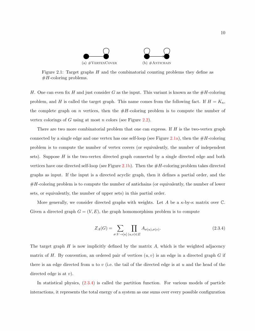
(a) #VertexCover (b) #Antichain

Figure 2.1: Target graphs H and the combinatorial counting problems they define as#H-coloring problems.

H. One can even fix H and just consider G as the input. This variant is known as the #H-coloring

problem, and H is called the target graph. This name comes from the following fact. If H = Kn,

the complete graph on n vertices, then the #H-coloring problem is to compute the number of

vertex colorings of G using at most n colors (see Figure 2.2).

There are two more combinatorial problem that one can express. If H is the two-vertex graph

connected by a single edge and one vertex has one self-loop (see Figure 2.1a), then the #H-coloring

problem is to compute the number of vertex covers (or equivalently, the number of independent

sets). Suppose H is the two-vertex directed graph connected by a single directed edge and both

vertices have one directed self-loop (see Figure 2.1b). Then the #H-coloring problem takes directed

graphs as input. If the input is a directed acyclic graph, then it defines a partial order, and the

#H-coloring problem is to compute the number of antichains (or equivalently, the number of lower

sets, or equivalently, the number of upper sets) in this partial order.

More generally, we consider directed graphs with weights. Let A be a κ-by-κ matrix over C.

Given a directed graph G = (V,E), the graph homomorphism problem is to compute

ZA(G) =∑

σ:V→[κ]

∏(u,v)∈E

Aσ(u),σ(v). (2.3.4)

The target graph H is now implicitly defined by the matrix A, which is the weighted adjacency

matrix of H. By convention, an ordered pair of vertices (u, v) is an edge in a directed graph G if

there is an edge directed from u to v (i.e. the tail of the directed edge is at u and the head of the

directed edge is at v).

In statistical physics, (2.3.4) is called the partition function. For various models of particle

interactions, it represents the total energy of a system as one sums over every possible configuration

11

(a) q = 2 (b) q = 3 (c) q = 4

Figure 2.2: Target graph H for counting q-colorings for q ∈ 2, 3, 4 as an #H-coloringproblem.

(a) q = 2 (b) q = 3 (c) q = 4

Figure 2.3: Target graph H for counting q-particle Widom-Rowlinson configurationsfor q ∈ 2, 3, 4 as an #H-coloring problem.

(a) q = 2 (b) q = 3 (c) q = 4

Figure 2.4: Target graph H for counting q-type Beach model configurations for q ∈2, 3, 4 as an #H-coloring problem.

12

of the particles. The Ising model [83] corresponds to the partition function with matrix A =[λ 11 λ

]for a parameter λ that can take any positive real number. The Ashkin-Teller Model [2] corresponds

to the partition function with matrix A =

[a b c db a d cc d a bd c b a

]for parameters a, b, c, d that can take any

positive real numbers. The Potts model [112] corresponds to the partition function with matrix

A = Jn + (λ− 1)In, where Jn is the n-by-n matrix of all 1’s and In is the n-by-n identity matrix.

Once again, λ is a parameter that can take any positive real number.

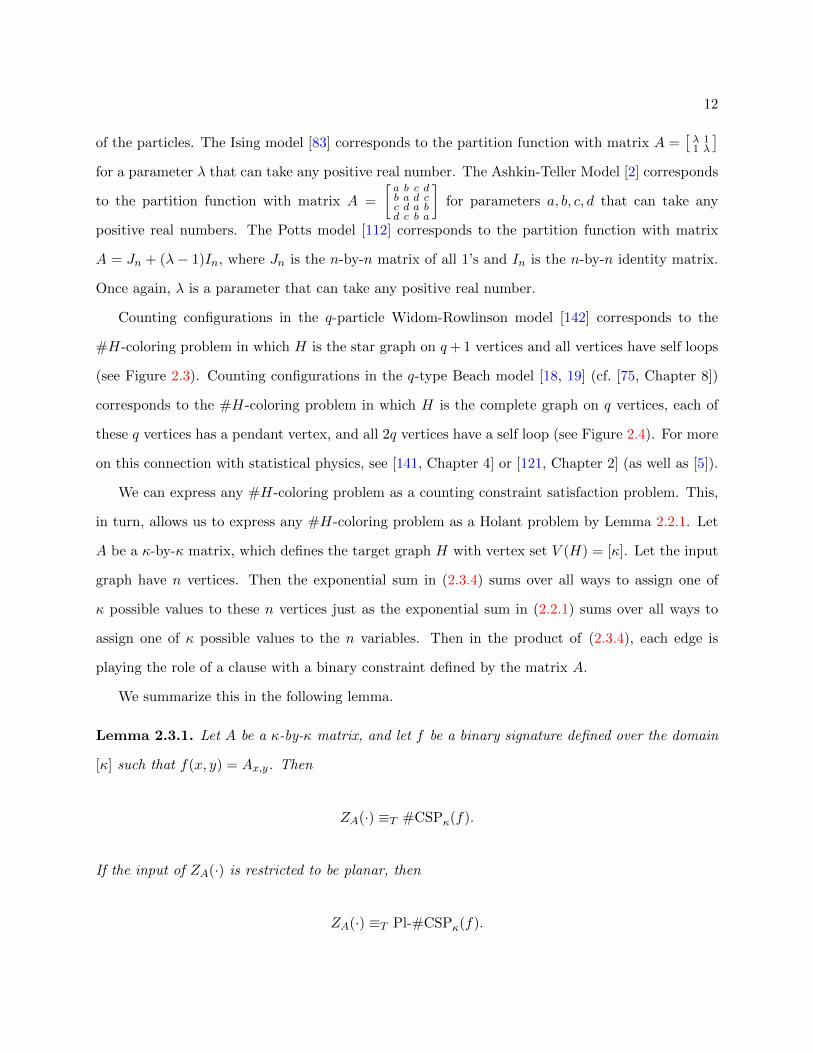
Counting configurations in the q-particle Widom-Rowlinson model [142] corresponds to the

#H-coloring problem in which H is the star graph on q+ 1 vertices and all vertices have self loops

(see Figure 2.3). Counting configurations in the q-type Beach model [18, 19] (cf. [75, Chapter 8])

corresponds to the #H-coloring problem in which H is the complete graph on q vertices, each of

these q vertices has a pendant vertex, and all 2q vertices have a self loop (see Figure 2.4). For more

on this connection with statistical physics, see [141, Chapter 4] or [121, Chapter 2] (as well as [5]).

We can express any #H-coloring problem as a counting constraint satisfaction problem. This,

in turn, allows us to express any #H-coloring problem as a Holant problem by Lemma 2.2.1. Let

A be a κ-by-κ matrix, which defines the target graph H with vertex set V (H) = [κ]. Let the input

graph have n vertices. Then the exponential sum in (2.3.4) sums over all ways to assign one of

κ possible values to these n vertices just as the exponential sum in (2.2.1) sums over all ways to

assign one of κ possible values to the n variables. Then in the product of (2.3.4), each edge is

playing the role of a clause with a binary constraint defined by the matrix A.

We summarize this in the following lemma.

Lemma 2.3.1. Let A be a κ-by-κ matrix, and let f be a binary signature defined over the domain

[κ] such that f(x, y) = Ax,y. Then

ZA(·) ≡T #CSPκ(f).

If the input of ZA(·) is restricted to be planar, then

ZA(·) ≡T Pl-#CSPκ(f).

13

Chapter 3

Reductions

3.1 Gadget Constructions

3.1.1 Local Gadget Constructions via F-gates

A basic type of reduction is what might be generally known as a gadget construction. In the context

of Holant problems, we create “local” gadget constructions in order to realize a signature. Fix a set

F of signature over a domain D of size κ. We say a signature f is realizable or obtainable from F

if there is a gadget with some dangling edges such that each vertex is assigned a signature from F ,

and the resulting graph, when viewed as a black-box signature with inputs on the dangling edges,

is exactly f .

Formally, such a notion is defined by an F-gate [46]. An F-gate F is similar to a signature grid

(G, π) for Holant(F) except that G = (V,E,E′) is a graph with regular edges in E and m dangling

edges in E′. The dangling edges define external variables for the F-gate. They are ordered by

starting at the edge marked with a diamond and proceeding counterclockwise. (See Figure 3.1 for

an example.) Then the F-gate F defines the function

Γ(y1, . . . , ym) = Holantκ(G′, π′),

where (y1, . . . , ym) ∈ Dm is an assignment on the dangling edges, G′ is the graph obtained from G

14

Figure 3.1: An F-gate with 5 dangling edges.

after attaching the dangling end of a dangling edge ei ∈ E′ (which is assigned yi) to a new vertex

vei , and π(vei) = δyi is the function that outputs 1 when its input is yi and outputs 0 otherwise. We

call this function Γ the signature of the F-gate. We also call an F-gate a gadget. If the signature

of an F-gate is invariant under cyclic permutations of inputs, then we omit the diamond since it is

unnecessary. We say that such signatures are rotationally symmetric.

An F-gate is planar if the underlying graph can be embedded in the plane without edge crossings

and the dangling edges are in the outer face. Now suppose we have two signature sets F and G in

the context of a bipartite Holant problem Holantκ(F | G). Then an (F | G)-gate is an (F ∪G)-gate

such that the underlying graph is bipartite, the vertices in one part are assigned signatures from

F , and the vertices in the other part are assigned signatures from G. Furthermore, we say that

an (F | G)-gate is on the left (resp. on the right) if each vertex incident to a dangling edge is

assigned a signature from F (resp. G). A planar (F | G)-gate is both a planar (F ∪ G)-gate and an

(F | G)-gate.

Using F-gates, we can reduce one Holant problem to another.

Lemma 3.1.1. Let F be a set of signatures over a domain of size κ. If there exists an F-gate with

signature f , then

Holantκ(F ∪ f) ≤T Holantκ(F).

Similar statements hold for gadgets that are planar, bipartite, or both for Holant problems defined

over the same class of graphs.

Proof. Let F be an F-gate with signature f . Given an instance Ω of Pl-Holantκ(F ∪ f), we

replace every appearance of f by the F-gate F to obtain an instance Ω′ of Pl-Holantκ(F). Since

15

f is the signature of the F-gate F , the Holant values for these two signature grids are identical.

Furthermore, the size of F is a constant with respect to Ω, so the size Ω′ is only a constant factor

larger than Ω.

Even for a very simple signature set F , the signatures for all F-gates can be quite complicated

and expressive. Indeed, given a set F of signatures and another signature f , it is undecidable to

decide if there exists an F-gate with signature f [54, Theorem 2].

It is convenient to write a signature as a matrix. An immediate advantage is that a matrix

is more of a pictorial representation than a vector, which aids understanding. However, the more

important reason is to simplify the computation of a gadget’s signature.

Definition 3.1.2. Let f be a signature of arity n over a domain of size κ. The signature matrix of

f with parameter ` is an κ`-by-κn−` matrix for some integer 0 ≤ ` ≤ n in which the first ` inputs

(in order) are the row index and the remaining n−` inputs (in reverse order) are the column index.

If the arity of f is even, then the signature matrix of f , without specifying a parameter, is the

signature matrix of f with parameter ` = n2 and is denoted by Mf .

The purpose of reversing the order of the column index is so that we can use matrix product

in some of our gadget computations. If f = (w, x, y, z) of arity 2 over the Boolean domain, then

Mf = [w xy z ]. If g is a signature of arity 4 over the Boolean domain with g(w, x, y, z) = gwxyz, then

Mg =

g0000 g0010 g0001 g0011

g0100 g0110 g0101 g0111

g1000 g1010 g1001 g1011

g1100 g1110 g1101 g1111

.

A signature matrix of a signature is also known as a Young flattening of a tensor [96, Section 3.4].

Let F be an F-gate with signature f of arity n. We often depict F with ` dangling edges protruding

to the left and n − ` dangling edges protruding to the right to aid in the mapping from F to the

signature matrix of f with parameter `. This is unnecessary is when f is symmetric, or more

generally, when f is invariant under cyclic permutations of its inputs.

16

(a) A counterclockwise rotation (b) Movement of signature matrix entries

Figure 3.2: The movement of the entries in the signature matrix of an arity 4 signatureover the Boolean domain under a counterclockwise rotation of the input edges. Entriesof Hamming weight 1 are in the dotted cycle, entries of Hamming weight 2 are in thetwo solid cycles (one has length 4 and the other one is a swap), and entries of Hammingweight 3 are in the dashed cycle.

For a signature f , a simple f-gate is a single vertex assigned f but with its inputs cyclically

permuted. Suppose f is of arity 4 and is defined over the Boolean domain. Consider an f-gate F

with signature f . If we rotate F counterclockwise by a quarter turn (or equivalently, if we cyclically

permute the inputs to f so that the first input becomes the last input), then we get a new f-gate

F ′ with signature f ′, and the signature matrix of f ′ is easily determined from the signature matrix

of f using Figure 3.2.

3.1.2 Domain Bundling

Consider the signature f = (1, 2, 3, 4, 5, 6, 7, 8, 9). I did not specify the arity of f or the domain size

over which it is defined. Is it possible to determine these two values given the fact that f has nine

outputs? It is not; this situation is ambiguous. Let n be the arity of f , and let k be the size of the

domain over which it is defined. What we know is that kn = 9, but there are two (positive integer)

solutions to this: either κ = 9 and n = 1 or κ = 3 and n = 2.

We can utilize this ambiguity to create a reduction that we call domain bundling.

Lemma 3.1.3. Suppose f is a signature of arity n over a domain of size κ. If κn = (κ′)n′

and

n | n′, then

Holantκ(f) ≤T Holantκ′(f′),

17

incorrect correct

Figure 3.3: Simple example of domain bundling. Both the correct as well as the naiveand incorrect way to connect the bundled edges are shown. As defined in the proof ofLemma 3.1.3, the graph G is above and the graph G′ is below (and on the right).

where f ′ has the same output values as f (when sorted lexicographically by input) but is viewed as

a signature of arity n′ over a domain of size κ′.

Proof. If (κ, n) = (κ′, n′), then there is nothing to prove, so assume otherwise. Then n < n′ and

κ > κ′ since n | n′.

Let G be an instance of Holantκ(f), which must be an n-regular graph. We construct an

instance G′ of Holantκ′(f′), which must be an n′-regular graph. The vertices in G′ are same as

the vertices in G. Each edge in G corresponds to n′

n edges in G′ between the same pair of vertices.

These n′

n edges, which each take one of κ′ possible assignments, simulate the κ possible assignments

in G since κ = (κ′)n′n . It remains to ensure that the inputs of f ′ at each vertex map correctly to

the variables on its incident edges.

By convention, the inputs of a signature map to the variables on its incident edges from first

to last (or equivalently, from most to least significant) as one traverses the edges counterclockwise

in some (not necessarily planar) embedding in the plane from specified initial edge. Consider two

incident vertices in G by an edge e. The variable on this edge takes κ possible values and of course

the two copies of f assigned to the two incident vertices agree on the meaning of these κ values. But

in G′, care must be taken to ensure that the two copies of f ′ agree on the meaning of assignments

to the corresponding n′

n incident edges. If they were connected in parallel in a planar way, then the

order that one copy of f ′ would interpret the κ = (κ′)n′n assignments to these n′

n edges would be

exactly opposite to the order that the other copy of f ′ would interpret them. To fix this, we connect

18

the edges to these vertices in the opposite order. At each vertex, the (cyclic) order is determined

by a counterclockwise traversal of the vertex.

Example 3.1.4. Consider the graph G at the top of Figure 3.3. Suppose the signature assigned to

both vertices is f = (f0, f1, f2, f3, f4, f5, f6, f7) of arity 1 over a domain of size 8. The Holant of

this graph is

f20 + f2

1 + f22 + f2

3 + f24 + f2

5 + f26 + f2

7 .

We can also view (f0, f1, f2, f3, f4, f5, f6, f7) as a signature f ′ of arity 3 over a domain of size 2.

If we assign f ′ to both vertices in the graph in the lower left of Figure 3.3, then the Holant is

f20 + f1f4 + f2

2 + f3f6 + f4f1 + f25 + f6f3 + f2

7 .

This Holant differs from the previous Holant because the three bundled edges were connected in

the “wrong” order. In contrast, if we assign f ′ to both vertices in the graph in the lower right of

Figure 3.3, then the Holant is

f20 + f2

1 + f22 + f2

3 + f24 + f2

5 + f26 + f2

7 ,

just as it was before applying the domain bundling reduction.

If f ′ were a symmetric signature, then connecting the n′

n edges in any order yields the same

contribution from f ′ and thus the same Holant value. In particular, one can put the edges in

parallel in a planar way, which gives a planar reduction.

Corollary 3.1.5. Let the situation be as in Lemma 3.1.3. If f ′ is symmetric, then

Pl-Holantκ(f) ≤T Pl-Holantκ′(f′).

I introduced the idea of domain bundling in the context of a single signature. However, we

typically apply this argument to multiple signatures in a bipartite graph. The proof for the bipartite

case is essentially the same as the proof of Lemma 3.1.3 when the bipartite restriction is absent.

19

Lemma 3.1.6. Suppose f (resp. g) is a signature of arity n (resp. m) over a domain of size κ. If

κn = (κ′)n′

and n | n′ as well as κm = (κ′)m′

and m | m′, then

Holantκ(f | g) ≤T Holantκ(f ′ | g′),

where f ′ (resp. g) has the same output values as f (resp. g) (when sorted lexicographically by input)

but is viewed as a signature of arity n′ (resp. m′) over a domain of size κ′.

3.2 Equivalent Expressions of the Same Problem

Some counting problems can be expressed as a Holant problem in more than one way. The primary

way of mapping between these expressions is with a holographic transformation. Recently, another

mapping was found, which is given in Subsection 3.2.2.

3.2.1 Holographic Transformation

A holographic transformation is the primary way of showing that two Holant problems with different

expressions are actually the same. Surely you already know the simplest example of this: in a

graph, the number of vertex covers is equal to the number of independent sets. The proof is that

the complement of one type of set is the other. At the vertex level, the complement exchanges the

assignments of 0 and 1.

A holographic transformation puts the assignments of 0 and 1 into a superposition much like

the states of a qubit in quantum computing. However, quantum computation is not required—or

even any computation at all. Just like the example with vertex covers and independent sets, we are

merely describing a mathematical proof that two different looking problems are actually the same.

We are undergoing a change of basis and viewing the problem from this new perspective.

To formally introduce the idea of holographic reductions, it is convenient to consider bipartite

graphs. For a general graph, we can always transform it into a bipartite graph while preserving the

Holant value as follows. For each edge in the graph, we replace it by a path of length two. (This

operation is called the 2-stretch of the graph and yields the edge-vertex incidence graph.) Each

20

new vertex is assigned the binary Equality signature (=2) = [1, 0, 1].

For a κ-by-κ matrix T and a signature set F , define TF = g | ∃f ∈ F of arity n, g = T⊗nf,

and similarly for FT , where the tensor product denoted by ⊗ is the Kronecker product. Whenever

we write T⊗nf or TF , we view the signatures as column vectors; similarly for fT⊗n or FT as row

vectors.

Let T be an invertible κ-by-κ matrix. The holographic transformation defined by T is the

following operation: given a signature grid Ω = (H,π) of Holant(F | G), for the same bipartite

graph H, we get a new grid Ω′ = (H,π′) of Holant(FT | T−1G) by replacing each signature in F

or G with the corresponding signature in FT or T−1G. Then by a result typically called Valiant’s

Holant Theorem [132] (see also [25]), the Holant value has not changed. His proof is for domain

size κ = 2, but also holds for any domain size. We state this as a lemma and provide a proof.

Lemma 3.2.1. Let F and G be sets of complex-valued signatures over a domain of size κ. Suppose

Ω is a bipartite signature grid over (F | G). If T ∈ GLκ(C), then

Holantκ(Ω;F | G) = Holantκ(Ω′;FT | T−1G),

where Ω′ is the corresponding signature grid over (FT | T−1G).

Proof. We modify Ω = Ω0 in several steps until it becomes Ω′ = Ω3. In each step, the Holant value

is unchanged. We illustrate our proof in Figure 3.4.

Let G = (U, V,E) be the graph underlying Ω = Ω0. Vertices in U are assigned signatures in F

by π while vertices in V are assigned signatures in G by π. We do the following operations for each

edge in E. Let e = (u, v) ∈ E be an edge with endpoints u ∈ U and V ∈ V . Initially, Figure 3.4a

depicts the neighborhood of u and v in Ω = Ω0. In this example, both u and v are incident to three

other edges but the vertices incident to the other ends of these edges are not shown.

We do the following operations for each edge in E. Let e = u, v ∈ E be an edge with endpoints

u ∈ U and V ∈ V . We subdivide e and assign =2 to the new vertex w. This increases the number

of terms in the Holant sum by a factor of 3. All original terms still appear and all new terms are 0.

Let the resulting signature grid be Ω1. See Figure 3.4b.

21

f g

(a) Ω = Ω0

=f g

= =

= =

= =

(b) Ω1

Figure 3.4: Neighborhood around two adjacent vertices.

22

f gTT

T

T

T−1T−

1

T−1

T−

1

T−

1

T−1

T−

1

T

T

T

(c) Ω2

f gT

TT

T

T−1

T−

1

T−1

T−

1

T−

1

T−1

T−

1

TT

T

(d) Ω3

Figure 3.4: Neighborhood around two adjacent vertices.

23

Then we subdivide w to get two adjacent vertices wu and wv so that we now have a path

(u,wu, wv, v). Let fu (resp fv) be the signature whose signature matrix is T (resp. T−1). We assign

fu (resp. fv) to wu (resp. wv). If T is not a symmetric matrix, then fu and fv are not symmetric

and it matters which edge corresponds to which input. The first input for fu (resp. fv) corresponds

to the edge u,wu (resp. wu, wv). Let the resulting signature grid be Ω2. See Figure 3.4c,

which indicates the first inputs of fu and fv by the rotation of T and T−1 (instead of the standard

notation of putting a diamond on the edge corresponding to the first input). Their first input is to

their left. If we contract the edge wu, wv within the dashed box, then we get back Ω1. Thus, the

Holant value has not changed.

Now Ω3 in Figure 3.4d is actually the same as Ω2. To get Ω4 = Ω′, we contract u,wu and

wv, v. After doing so, we once again have the graph G. What has changed is the assignment to

each vertex. The vertex u is now assigned fT⊗4, and the vertex v is now assigned (T−1)⊗4g.

In general, the new assignment to each vertex is the transformed signature in FT or T−1G

respectively, as claimed.

Therefore, an invertible holographic transformation does not change the complexity of the

Holant problem in the bipartite setting. Furthermore, there is a special kind of holographic trans-

formation, the orthogonal transformation, that preserves the binary equality and thus can be used

freely in the standard setting. For κ = 2, this first appeared in [45] as Theorem 2.2. We also state

it as a lemma.

Lemma 3.2.2. Let F be a set of complex-valued signatures over a domain of size κ. Suppose Ω is

a signature grid over F . If H ∈ Oκ(C), then

Holantκ(Ω;F) = Holantκ(Ω′;HF),

where Ω′ is the corresponding signature grid over HF .

We use Lemma 3.2.1 and Lemma 3.2.2 to reduce between both hard problems and easy problems.

Some of our reductions between easy problems use the following definition.

24

Definition 3.2.3. Let F be any set of symmetric, complex-valued signatures over a domain of

size κ. We say F is C -transformable if there exists a T ∈ GLκ(C) such that (=2)T⊗2 ∈ C and

F ⊆ TC .

This definition is important because if Holantκ(C ) is tractable over any set of graphs, then

Holantκ(F) is tractable over the same set of graphs for any C -transformable set F .

Lemma 3.2.4. Let F be any set of symmetric, complex-valued signatures over a domain of size κ.

If F is C -transformable, then

Holantκ(F) ≤T Holantκ(C ),

where both problems are defined over the same set of graphs.

3.2.2 Another Identity

Until recently, every pair of Holant problems with the same output for every input were known to

have a holographic transformation between them (except for some trivial examples). Then in [29,

Subsection 4.3], we made the following observation.

Lemma 3.2.5. Let x and y be indeterminates. Then for every (2, 4)-regular bipartite graph G,

Holant2(G; [0, 1, 0] | [x, y, 1, 0, 0]) = Holant2(G; [0, 1, 0] | [0, 0, 1, 0, 0])

as polynomials in x and y.

Proof. Consider Holant2(G; [0, 1, 0] | [x, y, 1, 0, 0]) for any (2, 4)-regular bipartite graph G, which is

a polynomial p(x, y) in the indeterminates x and y. Because [0, 1, 0] is the only signature on the

left, any nonzero term in the Holant sum must assign 1 to exactly half of the edges in G. On the

right side, if some copy of [x, y, 1, 0, 0] contributes an x or y in some assignment, then less than

half of its incident edges are assigned 1. To compensate, some other copy of [x, y, 1, 0, 0] must have

more than half of its incident edges assigned 0, so it contributes a factor of 0. Thus p(x, y) is a

constant, so it is equal to any evaluation, including (x, y) = (0, 0) as claimed.

25

G = G0 G1 G2

` `

``

G`

Figure 3.5: Some graphs obtained from an initial graph G in the proof of Lemma 3.3.1.

For all x, y ∈ C, there is no holographic transformation between these two Holant problems.

This is the first counterexample involving non-unary signatures in the Boolean domain (i.e. κ = 2)

to the converse of Lemma 3.2.2, which provides a negative answer to a conjecture made by Xia

in [143, Conjecture 4.1]. This result clearly generalizes to similarly defined signatures of even arity

on the right.

3.3 Polynomial Interpolation

Valiant [125] initiated the study of counting problems by defining the class #P. Then to explain

the apparent intractability of counting perfect matchings, he proved that this problem is #P-hard

(under polynomial-time Turing reductions). Immediately after, he initiated the use of polynomial

interpolation as a technique to obtain reductions between counting problems. This is a powerful tool

in the study of counting problems that makes it possible to prove complexity dichotomy theorems.

Let me begin with an example from Valiant’s paper [125, reduction 6 in the proof of Theorem 1].

Lemma 3.3.1. #PerfectMatching ≤T #Matching

Proof. Let G = (V,E) be a graph. We want to determine the number of perfect matchings in G

assuming that we have an oracle to count matchings.

For integers 0 ≤ ` ≤ n, let G` be the following modification of G. For each vertex v ∈ V , we

add a new vertex vk for all 1 ≤ k ≤ `. Then we add an edge between v and vk for all 1 ≤ k ≤ `.

See Figure 3.5 for some examples of these graphs beginning with a specific graph G.

Let mk be the number of matchings in G that omit k vertices. Then we can express the number

26

p(x) = 2x3−3x2−17x+ 10

−2 −1 1 2 3 4

−15

15

30

x

p(x)

Evaluate

x ∈ 1, 2, 3, 4

Interpolate

Figure 3.6: Interpolation is the inverse of evaluation.

of matchings in G` asn∑k=0

(1 + `)kmk = #Matching(G`).

This is because a matching M of size k in G can be extended to (1 + `)k matchings in G`. Each

vertex that is not matched by M has 1 + ` possibilities: it can remain unmatched or it can be

matched with any of its new ` neighbors in G`. These choices are independent for each vertex,

hence the exponent of k.

We collect these equations to form the linear system

(1 + 0)0 (1 + 0)1 · · · (1 + 0)n

(1 + 1)0 (1 + 1)1 · · · (1 + 1)n

......

. . ....

(1 + n)0 (1 + n)1 · · · (1 + n)n

m0

m1

...

mn

=

#Matching(G0)

#Matching(G1)

...

#Matching(Gn)

.

Using our oracle, we know the right side. On the left, the coefficient matrix is Vandermonde. It

is invertible because the entries in the second column are distinct. Therefore, we can invert this

matrix and solve for the unknown mk’s. Then m0, the number of matchings in G that omit no

vertices, is the number of perfect matchings G as desired.

27

The word “polynomial” did not appear in this proof, so what makes it an example of polynomial

interpolation? The polynomial is implicit; it is p(x) =∑n

k=0mkxk. Asking our oracle for the

number of matchings in G` is like evaluating p(x) at 1 + `. Polynomial interpolation is the process

of converting from points and their evaluations to the coefficients of the polynomial being evaluated

(see Figure 3.6), which is what this proof did.

Since our n+1 evaluation points are distinct, we can recover the coefficients of p(x). Given these

coefficients, our reduction can proceed by computing any polynomial-time computable function of

them. However, it is often the case that we are interested in some evaluation of the interpolated

polynomial. In the proof of Lemma 3.3.1, we evaluated the interpolated polynomial at 0 to obtain

p(0) = m0.

Now for an example where the polynomial is quite explicit. The chromatic polynomial, which is

denoted by χ(G;λ), is the unique polynomial satisfying χ(G;λ) = #λ-VertexColoring(G) for

all λ ∈ N. That is, it is the unique polynomial that evaluates to the number of vertex colorings of G

using at most λ colors when λ is a natural number. A nice exposition of the chromatic polynomial

can be found in [82].

The following example of polynomial interpolation is a dichotomy theorem for the chromatic

polynomial. The reduction we use comes from Linial [103] and the dichotomy was first explicitly

stated in [86]. Let χ(λ) be the problem of evaluating χ(G;λ) on an input graph G.

Theorem 3.3.2. Let λ ∈ C. Then χ(λ) is #P-hard unless λ ∈ 0, 1, 2, in which case, the problem

is computable in polynomial time.

Proof. If λ = 0, then χ(G,λ) = 00 = 1 if G has no vertices and is 0 otherwise. If λ = 1, then

χ(G,λ) = 1 if G has no edges and is 0 otherwise. If λ = 2, then χ(G,λ) = 2k if G is bipartite with

k connected components and is 0 otherwise.

Now suppose λ /∈ 0, 1, 2. We reduce from χ(3), which is #P-hard (see, for example [103,

Main Theorem, Case (6)] or [4, Proposition 5]). Let G be a graph with n vertices, and let Kt be

the complete graph on t vertices. We use G+Kt to denote the graph obtained from G by adding

28

Kt and all possible edges between the vertices of G and the vertices of Kt. Then clearly

λ(λ− 1) · · · (λ− t+ 1)χ(G;λ− t) = χ(G+Kt;λ).

when λ ∈ N. Thus, it must also hold as an equation of polynomials when considering λ as an

indeterminate. After rearranging, we have

χ(G;λ− t) =1

λ(λ− 1) · · · (λ− t+ 1)χ(G+Kt;λ). (3.3.1)

If λ ≥ 3 is an integer, then by setting t = λ − 3, we can directly solve for χ(G; 3) via (3.3.1).

Otherwise, λ /∈ N. Then using (3.3.1), we can compute χ(G;λ − t) for all 0 ≤ t ≤ n. From these

evaluations, we can interpolate the coefficients of χ(G; Λ) and evaluate it at Λ = 3.

The heart of polynomial interpolation as a reduction technique is finding an equation like (3.3.1).

On the left, we have the original graph G with some different evaluation point λ′. On the right,

we have the original evaluation point λ with some different graph G′. The main question is what

to pick for G′? It must be part of an infinite family because the degree of the polynomial being

interpolated grows with the size of G. The sizes of the graphs in this family must not grow too

quickly so that we can construct them in polynomial time. And finally, each graph in the family

must be expressible using the original graph G for some distinct evaluation point λ′.

To this end, it is typically best to minimize the sizes of these graphs. Additional vertices and

edges contribute terms to an equation like (3.3.1) that restrict the usefulness of the reduction. For

example, one could say that the kth vertex and its incident edges added to G in the construction

of G+Kt (for 0 ≤ k ≤ t) contribute a factor of 1λ−k+1 to the right side of (3.3.1). Because of these

factors, the interpolation fails when λ ∈ N. After adding the (λ + 1)th vertex and its edges, the

equation breaks down. The right side is no longer well defined because of a division by 0.

The proofs of both Lemma 3.3.1 and Theorem 3.3.2 involve interpolation of a single variable

polynomial. After homogenizing, they become homogeneous polynomials in two variables. For such

homogeneous polynomials of degree d, interpolation requires at least d + 1 evaluations, and d + 1

evaluations suffice iff, when viewed as length-two vectors, these d + 1 points are pairwise linearly

29

G G3

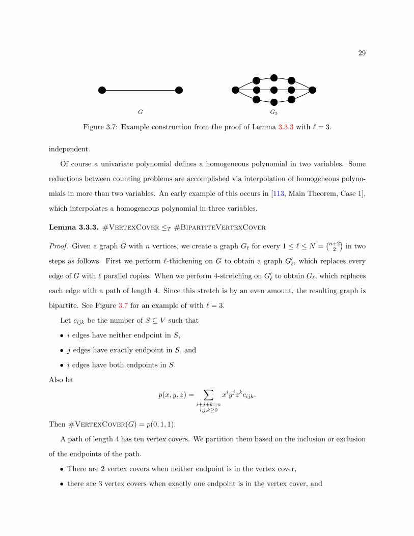
Figure 3.7: Example construction from the proof of Lemma 3.3.3 with ` = 3.

independent.

Of course a univariate polynomial defines a homogeneous polynomial in two variables. Some

reductions between counting problems are accomplished via interpolation of homogeneous polyno-

mials in more than two variables. An early example of this occurs in [113, Main Theorem, Case 1],

which interpolates a homogeneous polynomial in three variables.

Lemma 3.3.3. #VertexCover ≤T #BipartiteVertexCover

Proof. Given a graph G with n vertices, we create a graph G` for every 1 ≤ ` ≤ N =(n+2

2

)in two

steps as follows. First we perform `-thickening on G to obtain a graph G′`, which replaces every

edge of G with ` parallel copies. When we perform 4-stretching on G′` to obtain G`, which replaces

each edge with a path of length 4. Since this stretch is by an even amount, the resulting graph is

bipartite. See Figure 3.7 for an example of with ` = 3.

Let cijk be the number of S ⊆ V such that

• i edges have neither endpoint in S,

• j edges have exactly endpoint in S, and

• i edges have both endpoints in S.

Also let

p(x, y, z) =∑

i+j+k=ni,j,k≥0

xiyjzkcijk.

Then #VertexCover(G) = p(0, 1, 1).

A path of length 4 has ten vertex covers. We partition them based on the inclusion or exclusion

of the endpoints of the path.

• There are 2 vertex covers when neither endpoint is in the vertex cover,

• there are 3 vertex covers when exactly one endpoint is in the vertex cover, and

30

• there are 5 vertex covers when both endpoints are in the vertex cover.

Thus,

#VertexCover(G`) = p(2`, 3`, 5`). (3.3.2)

This gives us a Vandermonde system that has full rank iff 2i3j5k 6= 2i′3j‘5k

′when i + j + k =

i′ + j′ + k′ = n but (i, j, k) 6= (i′, j′, k′), which is clearly the case. Therefore, we can interpolate

p(x, y, z) and evaluate it at p(0, 1, 1) to obtain the number of vertex covers of G.

Remark. Let Pn be the path graph of length n. It is straightforward to verify that the vertex

covers of P4 can be partitioned into the triple (2, 3, 5) as claimed in the proof. One can derive this

triple by observing that the vertex covers of path graphs satisfy the recurrence relation

#VertexCover(Pn) = #VertexCover(Pn−1) + #VertexCover(Pn−2),

the same recurrence relation as the Fibonacci numbers. Let Fn be the nth Fibonacci number. The

(initial) triple of vertex covers for P1 is (0, 1, 1) = (F0, F1, F2). Then the triple of vertex covers for

Pk is (Fk−1, Fk, Fk+1). The proof uses k = 4 since this is the smallest positive even number for

which the triple (Fk−1, Fk, Fk+1) gives a Vandermonde system of full rank.

For homogeneous polynomials of degree d in n variables, there is no known useful characteriza-

tion of when some minimum number of points (namely(d+n−1n−1

)points) can be used to interpolate

such polynomials. However, this does not prevent us from using special collections of points for

which we can prove that interpolation does succeed.

For reductions between Holant problems, we often use interpolation of homogeneous polynomials

in more than two variables. See Section 11.3 for an explanation of how this is done. In particular,

we say that a three numbers like 2, 3, and 5 satisfy the lattice condition (cf. Definition 11.3.3) if a

Vandermonde system like that in (3.3.2) is full rank.

31

Chapter 4

Tractable Signatures

This chapter contains most of what is known about tractable Holant problems and the signatures

that define them. Although I would say that we have a good understanding of the tractable cases,

many questions still remain. I pose them throughout the chapter as they arise.

Given a problem P covered by a complexity dichotomy, it is natural to ask if P is easy. This

question is called the meta question or the decidability problem of the dichotomy. If P is easy, a

second question arises: what is the efficient algorithm that solves P? Some of the open problems

in this chapter are about these meta questions. In this context, we only consider finite F since it

is the input to the problem.

4.1 Product Type

As a symmetric signature in the Boolean domain, the Equality signature =n of arity n is denoted

by [1, 0, . . . , 0, 1] with n−1 zeros. The Holant of a signature grid that only uses Equality signatures

is easy to compute. Each connected component contributes a factor of 2. Let’s generalize these

signatures while still being able to easily compute the Holant.

One way to generalize them is to allow weights. For a, b ∈ C, we call the signature [a, 0, . . . , 0, b]

a generalized Equality signature. Consider a signature grid that only uses such signatures. Each

connected component of size k contributes a factor of ak + bk if each Equality signature had the

same weights. A similar (but more complicated) expression exists if the weights were to vary.

32

Consider a different generalization. In addition to all of the Equality signatures, we also allow

the binary Disequality signature 6=2. Now what does each connected component contribute?

Well, if there is any cycle containing an odd number of 6=2, then the contribution is 0. Otherwise,

the contribution is again 2. Does this mean that we must inspect every cycle? No, and its a good

thing too, because that would take exponential time.

The key observation is that among the exponentially many edge assignments, there are at most

two that could contribute a nonzero value. Furthermore, we can use a propagation algorithm to

efficiently determine if these two assignments exists and find them when they do. Pick any edge

and fix its assignment to 0. Then in order for the incident signatures to contribute nonzero values,

the assignments to all adjacent edges is also fixed. We recurse on each fixed edge. If we encounter

an edge that is fixed to different assignments, then we have a contradiction and the Holant is 0.

Otherwise, we have determined a consistent assignment for the connected component containing

the edge we initially picked. The other consistent assignment is the complement of this one, but we

could also find it from first principles by fixing the assignment of the initial edge to 1 and running

the propagation algorithm again.

There are three other symmetric signatures that we could add: [0, 0], [1, 0], and [0, 1]. If [0, 0]

is used, then there are no assignments and the Holant is 0. If [1, 0] or [0, 1] is used, then any

connected component in which they appear has at most one assignment that could contribute a

nonzero value. This only makes our life easier.

The propagation algorithm also works for the following types of signatures that may have

weights and may not be symmetric.

Definition 4.1.1. Let f be a signature of arity n over the Boolean domain. Then f is a generalized

equality signature if n = 1 and f is [0, 0], [1, 0], [0, 1] (up to scale), or n ≥ 2 and

∃x ∈ 0, 1n, ∀y ∈ 0, 1n, f(y) = 0 ⇐⇒ y 6∈ x,x.

The last condition says that the support set of f contains precisely two complementary indices.

We generalize this once further to signatures over larger domain sizes.

33

Definition 4.1.2. For any integer κ ≥ 2, let f be a signature of arity n over the domain [κ]. Then

f is a generalized equality signature if n = 1 and | support(f)| ≤ 1, or n ≥ 2 and

∀i ∈ [n], ∀x ∈ [κ], | support(fxi=x)| = 1,

where fxi=x is the restriction of f to inputs with its ith input xi fixed to x. We use E to denote

the set of all generalized Equality signatures.

Remark. Definition 4.1.1 and Definition 4.1.2 are written so that all signatures in E are irreducible

according to Definition 5.3 in [31].

The last condition says that the support set of f contains precisely κ “disjoint” indices. They

are disjoint in the sense that each index differs from all others in every position. It is easy to see

that the tensor rank of each signature in E is at most the domain size κ over which it is defined.

For these signatures with a larger domain, we only need to modify the propagation algorithm

slightly. After picking the first edge, we consider fixing it each element in [κ]. In each connected

component, there are at most κ assignments that could contribute a nonzero value, and the prop-

agation algorithm will find any such assignment that exist. This gives the following result.

Theorem 4.1.3. Suppose κ ≥ 2 is the domain size. Then Holantk(E ) is computable in polynomial

time.

We are supposed to be defining the product-type signatures, but the word “product” has yet

to occur. There is one more generalization, and it uses the term “product”.

Definition 4.1.4. A signature is of product type if it is the tensor product of signatures from E

with any ordering of inputs. We use P to denote the set of all product-type signatures.

In other words, P is the closure of E under tensor products and reordering of inputs. Tensor

products and reordering of inputs using signatures from a set F is a special case of an F-gate. Specif-

ically, it is the special case when there are no internal edges. it is the special case with no internal

edges. Thus, we obtain the following corollary by combining Theorem 4.1.3 and Lemma 3.1.1.

34

Corollary 4.1.5. Suppose κ ≥ 2 is the domain size. Then Holantk(P) is computable in polynomial

time.

By combining Corollary 4.1.5 and Lemma 3.2.4, we obtain another corollary.

Corollary 4.1.6. Let F be any set of complex-valued signatures over a domain of size κ. If F is

P-transformable, then Holantk(F) is computable in polynomial time.

Definition 3.3 in [53] contains the original definition of P (over the Boolean domain) and uses

a slightly different notion of the term “product”. Now we list the symmetric signatures in P over

the Boolean domain.

Proposition 4.1.7 (Lemma A.1 in [81]). Let f ∈P be a symmetric signature. Then there exists

a, b ∈ C and n ∈ Z+ such that f takes one of the following forms:

1. [a, b]⊗n;

2. [0, a, 0];

3. [a, 0, . . . , 0, b] = a[1, 0]⊗n + b[0, 1]⊗n.

Let F be a finite set of complex-valued signatures over the Boolean domain. Then [34] gave a

polynomial-time algorithm to decide if F is P-transformable. When it is, the algorithm also finds

a corresponding transformation. Further suppose that F only contains symmetric signatures, and

these signatures are given in their exponentially more succinct representation, Then [34] also gave

a polynomial-time algorithm to decide if F is P-transformable. When it is, the algorithm also

finds a corresponding transformation. Many questions remain about deciding P-transformability.

I state the central ones as open problems.

Open Problem 4.1.8. Let F and G be finite sets of complex-valued signatures over a domain of

size κ ≥ 2.

1. Is there an algorithm to decide if there exists a T ∈ GLκ(C) such that GT ⊆P and F ⊆ TP?

2. If so, is there an algorithm to find such a T?

3. In either case, if an algorithm exists, then does a polynomial-time algorithm exist?

The same questions when F and G contain only symmetric signatures, and these signatures are

given in their exponentially more succinct representation.

35

To repeat, the results in [34] answer these questions in the affirmative in the special case that

κ = 2 and G = =2.

4.2 Affine

Definition 4.2.1. Let f by a signature of arity n with inputs x1, . . . , xn over the Boolean domain.

Then f is affine if it has the form

λ · χAx=0 · iq(x),

where λ ∈ C, x = (x1, x2, . . . , xn, 1)ᵀ, A is a matrix over Z2, χ is a 0-1 indicator function such

that χAx=0 is 1 iff Ax = 0, and q ∈ Z4[x] is a quadratic polynomial with even coefficients on cross

terms. We use A to denote the set of all affine signatures.

Of course the number of columns in the matrix A must be n+ 1 but there is no restriction on

the number of rows. It is permissible that A is the all-zero matrix so that χAx=0 = 1 holds for all

x. The name affine comes from the fact that solutions to Ax = 0 (and thus the support of f) form

an affine subspace.

The next result shows how the nontrivial symmetric affine signatures have a compact expression.

When viewed as tensors, this shows that they have tensor rank (at most) 2.

Proposition 4.2.2. Let f ∈ A be a unary signature or a non-degenerate symmetric signature.

Then f is an element in one (or possibly more if arity(f) ≤ 2) of the following three sets:

F1 =λ(

[1, 0]⊗k + ir[0, 1]⊗k)| λ ∈ C, k ∈ Z+, r ∈ 0, 1, 2, 3

;

F2 =λ(

[1, 1]⊗k + ir[1,−1]⊗k)| λ ∈ C, k ∈ Z+, r ∈ 0, 1, 2, 3

;

F3 =λ(

[1, i]⊗k + ir[1, −i]⊗k)| λ ∈ C, k ∈ Z+, r ∈ 0, 1, 2, 3

.

Proposition 4.2.3. Let f ∈ A be a unary signature different from [0, 0] or a non-degenerate

symmetric signature. If the first nonzero entry in f is 1, then f takes one of the following forms:

36

1. [1, 0, . . . , 0,±1]; (F1, r = 0, 2)

2. [1, 0, . . . , 0,±i]; (F1, r = 1, 3)

3. [1, 0, 1, 0, . . . , 0 or 1]; (F2, r = 0)

4. [1,−i, 1,−i, . . . , 1 or −i]; (F2, r = 1)

5. [0, 1, 0, 1, . . . , 0 or 1]; (F2, r = 2)

6. [1, i, 1, i, . . . , i or 1]; (F2, r = 3)

7. [1, 0,−1, 0, 1, 0,−1, 0, . . . , 0 or 1 or −1]; (F3, r = 0)

8. [1, 1,−1,−1, 1, 1,−1,−1, . . . , 1 or −1]; (F3, r = 1)

9. [0, 1, 0,−1, 0, 1, 0,−1, . . . , 0 or 1 or −1]; (F3, r = 2)

10. [1,−1,−1, 1, 1,−1,−1, 1, . . . , 1 or −1]. (F3, r = 3)

Because of Proposition 4.2.2, I used to wonder if all affine signatures had tensor rank (at most) 2.

This is not the case. The affine signature f ′ introduced below (before Lemma 4.2.14) has tensor

rank at least 4. This follows from [96, Exercise 2.6.6.3] since its signature matrix has full rank. I still

wonder though if there is some connection between the complexity of a signature f (equivalently,

the complexity of contracting tensor networks only involvoing f) and the tensor rank of f . For

example, Hastad [76] proved that determining the rank of an aribtray tensor is NP-hard. Maybe

determining the rank of a tensor in A is easier.

Open Problem 4.2.4. Given an element of A , what is the complexity of determining its tensor

rank? Can this be done in polynomial time? If so, can one do better and give a classification in

terms of tensor rank or border rank?

After normalizing, it is easy to count the symmetric affine signatures that are not identically

zero. For arity 1, there are six such signatures ([1, 0], [0, 1], [1,±1], [1,±i]). For larger arities,

a degenerate symmetric affine signature that is not identically zero is a tensor power of one of

these six. Then for arity 2, there are nine non-degenerate symmetric affine signatures up to scale

([1, 0,±1], [1, 0,±i], [1,±i, 1], [1, 1,±1], [0, 1, 0]). For arity at least 3, there are twelve non-degenerate

symmetric affine signatures up to scale, which are listed above.

For affine signatures that are not necessary symmetric, the situation is more complicated. It is

easy to count the possible quadratic polynomials with constant term 0 (there are 4n2(n2) possibili-

37

ties), and the number possible affine supports is also known [98] (there are∑n

k=0 2n−k∏k−1i=0

2n−2i

2k−2i

possibilities), but I don’t know how these two quantities “intersect” in Definition 4.2.1.

Open Problem 4.2.5. Determine the number of affine signatures up to scale over the Boolean

domain as a function of the arity.

Table 4.1: The number of affine signatures over the Boolean domain that are notidentically zero as a function of arity (according to my computer calculations). Withan AMD Phenom II processor and 3 GB of RAM, my computer outputs the last entryin just under 10 minutes. I am unable to compute the next entry due to lack of memory(since it is easier to write the algorithm that keeps everything in memory at once).

arity number

1 6

2 60

3 1080

4 36720

If it helps, one can restrict to signatures that are irreducible according to Definition 5.3 in [31].

I have written code in Mathematica to compute the affine signatures over the Boolean domain that

are not identically zero and with the first nonzero entry normalized to 1. The numbers I get are

given in Table 4.1. Neither this sequence nor this sequence with each number increased by 1 (to

account for the identically-zero signature) are in The On-Line Encyclopedia of Integer Sequences.

The affine signatures over the Boolean domain were originally defined in Definition 3.1 of [53].

This paper also proves their tractability.

Theorem 4.2.6 (Theorem 4.1 in [53]). Holant2(A ) is computable in polynomial time.

By combining theorem 4.2.6 and Lemma 3.2.4, we obtain the following corollary.

Corollary 4.2.7. Let F be any set of complex-valued signatures over the Boolean domain. If F is

A -transformable, then Holantk(F) is computable in polynomial time.

Definition 3.1 of [53] (for the affine signatures over the Boolean domain) is different from but

equivalent to Definition 4.2.1. My reason for using this alternative definition is to highlight the

similarity with the tractability result in [21]. After giving a definition for affine signatures over a

domain of size 3, I show how to use [21] to prove their tractability.

38

Definition 4.2.8. Let f by a signature of arity n with inputs x1, . . . , xn over the domain Z3. Then

f is affine if it has the form

λ · χAx=0 · e2πi3q(x),

where λ ∈ C, x = (x1, x2, . . . , xn, 1)ᵀ, A is a matrix over Z3, χ is a 0-1 indicator function such that

χAx=0 is 1 iff Ax = 0, and q ∈ Z3[x] is a quadratic polynomial. We still use A to denote the set

of all affine signatures.

Lemma 4.2.9. Holant3(A ) is computable in polynomial time.

Proof. Given an instance of Holant3(A ) with m edges, the output can be expressed as the sum-

mation of a single function F (x) = χAx=0 · e2πi3q(x), where x = (x1, . . . , xm). This is because A is

closed under multiplication. In polynomial time, we can solve the linear system Ax = 0 over Z3 to

determine if it is feasible. If it is infeasible, then F is identically zero, so the output is simply 0.

Otherwise, the linear system is feasible (including possibly vacuous). Without loss of generality,

we can assume that y1, . . . , yn ∈ x1, . . . , xm are independent variables over Z3 while all others

are dependent variables, where 0 ≤ n ≤ m. Each dependent variable can be expressed by an affine

linear form of y1, . . . , yn. We can substitute for all dependent variables in q(x), which gives a new

quadratic polynomial q′(y), where y = (y1, . . . , yn). Thus, we have

∑x1,...,xm∈Z3

χAx=0 · e2πi3q(x1,...,xm) =

∑y1,...,yn∈Z3

e2πi3q′(y1,...,yn). (4.2.1)

Then the right side of (4.2.1) is computable in polynomial time by Theorem 1 in [53].

The Equality signatures over the Z3 domain are examples of affine signatures. Their support

is defined by equating all variables, and their quadratic polynomial is the constant polynomial 0.

We give another, less-trivial example. Consider the signature

f(x, y, z) =

a x = y = z

c x 6= y 6= z 6= x

0 otherwise,

(4.2.2)

39

where a3 = c3. If a = c = 0, then this example is trivial, so assume otherwise. Then the support

of f is the affine subspace of Z3 defined by x + y + z = 0. Let ω = e2πi3 and let q c

a(x, y, z) =

λ ca(xy+ xz + yz) be a quadratic polynomial, where λ1 = 0, λω = 2, and λω2 = 1. Then aω

q ca

(x,y,z)

agrees with f when x+ y + z = 0. This gives the following corollary.

Corollary 4.2.10. Let a, c ∈ C. If f is defined as in (4.2.2), then Holant3(f) is computable in

polynomial time.

By combining Corollary 4.2.10 with Lemma 3.2.2, we have another corollary.

Corollary 4.2.11. Let a, c ∈ C. Suppose T ∈ O3(C). If f is defined as in (4.2.2), then

Holant3(T⊗3f) is computable in polynomial time.

Even though I have given a definition for affine signatures over a domain of size 3, this definition

has yet to be thoroughly tested.

Open Problem 4.2.12. Over a domain of size κ ≥ 3, determine the “right” definition of the affine

signatures.

The “right” definitions are the ones that fit like a glove in the statement of a powerful dichotomy

theorem. For the Boolean domain, there are plenty of dichotomy theorems to believe that Defini-

tion 4.2.1 is the “right” one. The dichotomy in [53] is probably the best example. Definition 4.2.8

is used to state a dichotomy theorem in Chapter 11. However, only the special case given in Corol-

lary 4.2.11 appears in the statement of that dichotomy theorem because only signatures of a rather

restricted form are considered.

Here is my guess as to the “right” definition of the affine signatures over a domain of size κ. If

κ is not a power of 2, then affine signatures are of the form λ ·χAx=0 · e2πiκq(x), where A is a matrix

over Zκ and q ∈ Zκ[x] is a quadratic polynomial. If κ is a power of 2, then affine signatures are of

the form λ · χAx=0 · e2πi2κq(x), where A is a matrix over Zκ and q ∈ Zκ[x] is a quadratic polynomial

with even coefficients on cross terms.

Open Problem 4.2.13. Given some definition of the affine signatures over a domain of size κ ≥ 3

(preferably the “right” one), determine the number of affine signatures up to scale over this domain

size as a function of the arity.

40

Table 4.2: The number of affine signatures over a domain of size 3 (as defined byDefinition 4.2.8) that are not identically zero as a function of arity (according to mycomputer calculations). The last line took just over 50 minutes to compute. Alsounable to compute the next entry due to lack of memory.

arity number

1 6

2 120

3 8400

I am not positive that Definition 4.2.8 is the “right” definition of the affine signatures over a

domain of size 3. Nonetheless, I have written code in Mathematica to compute the ones that are

not identically zero and with the first nonzero entry normalized to 1. The numbers I get are given

in Table 4.2. Again, neither this sequence nor this sequence with each number increased by 1 (to

account for the identically-zero signature) are in The On-Line Encyclopedia of Integer Sequences.

Now we give two examples of asymmetric affine signatures over the Boolean domain. Let

f ′(x1, x2, y1, y2) =

1 (x1, x2) = (y1, y2),

−1 (x1, x2) 6= (y1, y2).

(4.2.3)

This signature is affine over the Boolean domain since f ′(x1, x2, y1, y2) = (−1)q(x1,x2,y1,y2), where q

is the quadratic polynomial

q(x1, x2, y1, y2) = x1 + x2 + y1 + y2 + x1x2 + y1y2 + x1y2 + x2y1. (4.2.4)

Let

g′(x1, x2, y1, y2, z1, z2) =

1 (x1, x2) = (y1, y2) = (z1, z2),

0 otherwise.

(4.2.5)

This signature is affine over the Boolean domain since its support is defined by the affine equations

(x1, x2) = (y1, y2) = (z1, z2) and its quadratic polynomial is the constant polynomial 0.

Alternatively, we can view f ′(x1, x2, y1, y2) as a signature f(x, y) of arity 2 over a domain of

41

size 4, where x = (x1, x2) and y = (y1, y2). Then

f(x, y) =

1 x = y,

−1 x 6= y.

(4.2.6)

Similarly, we can view g′(x1, x2, y1, y2, z1, z2) as a signature g(x, y, z) of arity 3 over a domain of

size 4, where x = (x1, x2), y = (y1, y2), and z = (z1, z2). Then g = (=3). This gives the following

tractability result, which corresponds to a tractable case in the dichotomy theorem presented in

Chapter 11.

Lemma 4.2.14. If f is defined as in (4.2.6), then Holant4(f | =3) is computable in polynomial

time.

Proof. Let f ′ and g′ be defined as in (4.2.3) and (4.2.5) respectively. Then by Lemma 3.1.6, we

have

Holant4(f | =3) ≤T Holant2(f ′ | g′).

By ignoring the bipartite restriction, we further have

Holant2(f ′ | g′) ≤T Holant2(f ′, g′).

As demonstrated above, f ′ and g′ are both affine signatures over the Boolean domain, so we are

done by Theorem 4.2.6.

This highlights another difficulty with counting affine signatures over higher domains. I don’t

think that one should count f and g = (=3) as affine signatures (over a domain of size 4) when

trying to answer Open Problem 4.2.13. Instead, I would say that they are being simulated by affine

signatures over a domain of a different size (namely a domain of size 2). However, the Equality

signatures of all arities should be affine signatures over domains of all sizes, so g = (=3) is certainly

an affine signature over a domain of size 4 for the “right” definition of affine signatures.

Let F be a finite set of complex-valued signatures over the Boolean domain. Then [34] gave a

polynomial-time algorithm to decide if F is A -transformable. When it is, the algorithm also finds

42

a corresponding transformation. Further suppose that F only contains symmetric signatures, and

these signatures are given in their exponentially more succinct representation, Then [34] also gave

a polynomial-time algorithm to decide if F is A -transformable. When it is, the algorithm also

finds a corresponding transformation. Many questions remain about deciding A-transformability.

I state the central ones as open problems.

Open Problem 4.2.15. Let F and G be finite sets of complex-valued signatures over a domain

of size κ ≥ 2.

1. Is there an algorithm to decide if there exists a T ∈ GLκ(C) such that GT ⊆ A and F ⊆ TA ?

2. If so, is there an algorithm to find such a T?

3. In either case, if an algorithm exists, then does a polynomial-time algorithm exist?

The same questions when F and G contain only symmetric signatures, and these signatures are

given in their exponentially more succinct representation.

To repeat, the results in [34] answer these questions in the affirmative in the special case that

κ = 2 and G = =2.

4.3 Matchgate

Matchgates were introduced by Valiant [128, 127, 129] to give polynomial-time algorithms for a

number of counting problems over planar graphs.1 A matchgate is simply a gadget used to reduce

some counting problem to that of counting weighted perfect matchings. Over planar graphs, the

latter problem is computable in polynomial by Kasteleyn’s algorithm [89, 88].2

Let me give a simple example to explain this idea. The unweighted perfect matching signature

1Valiant’s matchgates in [128] sometimes contained edge crossings. However, this doesn’t mean that Valiant’sargument in [128] was able to simulate quantum circuits with edge crossings. Indeed, Valiant required that thequantum circuits only had “nearest neighbor interactions”, which means that there are no edge crossings. To allowedge crossings in matchgates is an attempt to increase their expressiveness. However, edge crossings do not increasethe expressiveness of matchgates. See [28], especially Section 5, for a proof of this.

2This algorithm is also called the FKT algorithm because it generalizes previous work by both Kasteleyn [87]and as well as Temperley and Fisher [120]. These two works both proved that the dimer model (i.e. countingperfect matchings) over two-dimensional lattices is “exactly solvable”, which essentially means that the number ofperfect matchings over such graphs has a mathematical expression that only involves polynomially many fundamentaloperations. The motivation for considering the two-dimensional (weighted) dimer model is that it expresses, after aholographic transformation, the Ising model as a special case.

43

Figure 4.1: Triangle gadget.

of arity 3 is [0, 1, 0, 0]. The problem Pl-Holant([0, 1, 0, 0]) is to count perfect matchings over planar

3-regular graphs. Of course this problem is computable in polynomial time. Then by Lemma 3.1.1,

Pl-Holant(f) is also computable in polynomial time for any [0, 1, 0, 0]-gate f .

Consider the gadget in Figure 4.1. We assign [0, 1, 0, 0] to all three vertices. Let g be the

signature of the resulting gadget. Then what is g? By the symmetry of the gadget, it is easy to

see that g is a symmetric signature, so we can write g = [g0, g1, g2, g3]. Because there is an odd

number of vertices in this gadget, we have g0 = g2 = 0. If exactly one vertex is matched externally

(which means that one dangling edge is assigned 1 and the other two dangling edges are assigned 0),

then there is one internal perfect matching (of size 1), so g1 = 1. If all three vertices are matched

externally (which means that all three dangling edges are assigned 1), then there is one internal

perfect matching (the empty matching of size 0), so g3 = 1 as well. Alternatively, assigning 0’s

to all internal edges is the only internal assignment such that the signature [0, 1, 0, 0] assigned to

each of the three vertices does not tribute a factor of 0. For this internal assignment, the three

vertices each contributes a factor of 1. Thus, g = [0, 1, 0, 1]. For this reason, g is called a matchgate

signature.

Definition 4.3.1. Let W be the set of all weighted matching signatures (that is, signatures with

output 0 on any input with Hamming weight different from 1). Then f is a matchgate signature if

it is the signature of some planar W -gate. We use M to denote the set of all matchgate signatures.

Said another way, the set M of matchgate signatures is the closure of W under the construction

of all possible planar W -gates. Therefore, by Lemma 3.1.1 and the FKT algorithm, we have the

following result.

Theorem 4.3.2. Pl-Holant(M ) is computable in polynomial time.

44

However, Definition 4.3.1 is not useful in checking if a given signature is a matchgate signature.

The work of Cai et al. [25, 26, 40] developed a theory to give a useful characterization of matchgate

signatures. See [28] for a self-contained account of this theory.

Here is an explicit list of the symmetric matchgate signatures.

Proposition 4.3.3. Let f ∈ M be a symmetric signature. Then there exists a, b ∈ C and n ∈ N

such that f takes one of the following forms:

1. [an, 0, an−1b, 0, . . . , 0, abn−1, 0, bn] (of arity 2n ≥ 2);

2. [an, 0, an−1b, 0, . . . , 0, abn−1, 0, bn, 0] (of arity 2n+ 1 ≥ 1);

3. [0, an, 0, an−1b, 0, . . . , 0, abn−1, 0, bn] (of arity 2n+ 1 ≥ 1);

4. [0, an, 0, an−1b, 0, . . . , 0, abn−1, 0, bn, 0] (of arity 2n+ 2 ≥ 2).

In the last three cases with n = 0, the signatures are [1, 0], [0, 1], and [0, 1, 0]. Any multiple of these

is also a matchgate signature.

Notice that every other entry is 0. This is a simple consequence of the fact that perfect matchings

contain an even number of vertices. The parity of a matchgate signature is even (resp. odd) if its

support is on entries of even (resp. odd) Hamming weight. More generally, a signature is said

to satisfy the parity condition if all entries of even Hamming weight are 0 or if all entries of

odd Hamming weight are 0. The nonzero entries of the symmetric matchgate signatures form a

geometric progression.

Another useful way to view the symmetric signature in M is via a low tensor rank decomposi-

tion. Such expressions make it easier to apply a holographic transformation. These expressions are

similar to those in Proposition 4.2.2 for the affine signatures over the Boolean domain. To state

these low rank decompositions, we use the following definition.

Definition 4.3.4. Let Sn be the symmetric group of degree n. Then for positive integers t and n

with t ≤ n and unary signatures v, v1, . . . , vn−t, we define

Symtn(v; v1, . . . , vn−t) =

∑π∈Sn

n⊗k=1

uπ(k),

where the ordered sequence (u1, u2, . . . , un) = (v, . . . , v︸ ︷︷ ︸t copies

, v1, . . . , vn−t).

45

Proposition 4.3.5. Let f ∈M be a symmetric signature of arity n. Then there exist a, b, λ ∈ C

such that f takes one of the following forms:

1. [a, b]⊗n + [a,−b]⊗n =

2[an, 0, an−2b2, 0, . . . , 0, bn] n is even,

2[an, 0, an−2b2, 0, . . . , 0, abn−1, 0] n is odd;

2. [a, b]⊗n − [a,−b]⊗n =

2[0, an−1b, 0, an−3b3, 0, . . . , 0, abn−1, 0] n is even,

2[0, an−1b, 0, an−3b3, 0, . . . , 0, bn] n is odd;

3. λ Symn−1n ([1, 0]; [0, 1]) = [0, λ, 0, . . . , 0];

4. λ Symn−1n ([0, 1]; [1, 0]) = [0, . . . , 0, λ, 0].

The first two items are decompositions of tensor rank (at most) 2. The last two items are

decompositions of tensor rank n. Furthermore, one can check that these signatures do indeed have

tensor rank n. However, they have border rank 2. (These facts follow from slight modifications to

the example and the reasoning for it in [96, Subsection 2.4.5]). I pose the corresponding question

for M as in Open Problem 4.2.4.

Open Problem 4.3.6. Given an element of M , what is the complexity of determining its tensor

rank? Can this be done in polynomial time? What about the same questions for border rank? If

so, can one do better and give a classification in terms of tensor rank or border rank?

By combining Theorem 4.3.2 with Lemma 3.2.4, we have the following corollary.

Corollary 4.3.7. Let F be any set of symmetric, complex-valued signatures in Boolean variables.

If F is M -transformable, then Pl-Holant(F) is computable in polynomial time.

In contrast with the product-type and affine signatures, there doesn’t seem to be a generalization

of M to larger domain sizes. Of course the signatures in M can simulate others defined over a

larger domain size by a domain bundling argument like Corollary 3.1.5. But the following questions

remain.

Open Problem 4.3.8. For a domain of size κ ≥ 3, what #CSPs are hard over general graphs but

tractable over planar graphs? Are any of these problems tractable for some reason other than by

reduction to Boolean domain Holant problems defined by signatures in M ?

46

Matchgates were not studied in isolation. The theory of matchgates was developed in con-

junction with the theory of holographic reductions (cf. Subsection 3.2.1). The initial holographic

reductions reduced to Holant problems using certain matchgate signatures over planar graphs (ei-

ther by Valiant [130, 131, 133] or Cai et al. [42, 43, 44, 41]). This resulted in an abundance of

counting problems over planar graphs with new polynomial-time algorithms. Although the phrase

“holographic algorithm” is meant to refer to any polynomial-time algorithm that uses a holographic

reduction, it became synonymous with polynomial-time algorithms with a holographic reduction

to matchgates (or more preciously, to Holant problems using matchgate signatures over planar

graphs).

Holographic reductions to Holant problems with product-type or affine signatures also exist [52,

47, 35, 80, 30, 34, 27]. To prove the dichotomy theorems just referenced, it is not necessary to obtain

characterizations of the A -, P-, or M -transformable signatures. The condition of transformability

arises naturally in the proof. However, the characterizations of transformability are useful in

answering the decidability question of these dichotomy theorems. The current understanding of

A - and P-transformability are discussed in the text surrounding Open Problem 4.1.8 and Open

Problem 4.2.15 respectively.

The corresponding questions for M with two sets of symmetric signatures were answered in

the affirmative by Theorem 4.1 in [43]. What remains open is the case in which the signatures

might not be symmetric (which tends to be easier since the input is exponentially larger than in

the symmetric case).

Open Problem 4.3.9. Let F and G be finite sets of complex-valued signatures over a domain of

size κ ≥ 2.

1. Is there an algorithm to decide if there exists a T ∈ GL2(C) such that GT ⊆M and F ⊆ TM ?

2. If so, is there an algorithm to find such a T?

3. In either case, if an algorithm exists, then does a polynomial-time algorithm exist?

The heart of the FKT algorithm is to find a Pfaffian orientation. For such an orientation,

the number of perfect matchings is the Pfaffian of the corresponding signed adjacency matrix.

Furthermore, The Pfaffian of such a matrix can be computed in polynomial time using efficient

47

algorithms for the determinant. What Kasteleyn proved in [89, 88] is that planar graphs have a

Pfaffian orientation and that one can be found in polynomial time.

Is there a larger class of graphs with a Pfaffian orientation that count be found in polynomial

time? The answer is yes! Little [104] proved that K3,3-free graphs have a Pfaffian orientation, and

Vazirani [134] showed how to find such an orientation in polynomial time. More recently, it was

shown how to count perfect matchings over K5-free graphs [118], and then over H-free graphs for

any graph H with a planar embedding that has at most one crossing [56], both in polynomial time.

However, these new results are not based on finding a Pfaffian orientation.

4.4 Vanishing

This section is about a tractable case called vanishing signatures. It was published in [29, 30].

Vanishing signatures were first introduced in [72] in the parity setting to denote signatures for

which the Holant value is always 0 modulo 2.

Definition 4.4.1. A set of signatures F is called vanishing if the value HolantΩ(F) is 0 for every

signature grid Ω. A signature f is called vanishing if the singleton set f is vanishing.

A simple lemma (Lemma 6.2 in [72]) from the parity setting also holds over any field F with

the same proof. It also works for signatures that may not be symmetric. Let f + g denote the

entry-wise addition of two signatures f and g with the same arity, i.e. (f + g)` = f` + g` for any

index `.

Lemma 4.4.2. Let F be a vanishing signature set. If f is the signature of an F-gate, then F ∪f

is also vanishing. If f, g ∈ F of the same arity, then F ∪ f + g is vanishing as well.

Obviously, any signature that is identically zero is vanishing. This is trivial. However, the

concept of vanishing signatures is not trivial. The unary signature [1, i] connected to another

[1, i] has a Holant value of 0. Consider a signature set F in which every signature of arity n is

degenerate. That is, every signature of arity n is a tensor product of unary signatures. Moreover,

for each signature, suppose that more than half of the unary signatures in the tensor product are

48

[1, i]. For any signature grid Ω with signatures from F , it can be decomposed into many pairs of

unary signatures. The total Holant value is the product of the Holant on each pair. Since more

than half of the unaries in each signature are [1, i], more than half of the unaries in Ω are [1, i]. Then

two [1, i]’s must be paired up. Hence Holant(Ω) = 0. Thus, all such signatures form a vanishing

set. We also observe that this argument holds when [1, i] is replaced by [1,−i].

These observations were the genesis for the complex-weighted Holant dichotomy in [30]. A

dichotomy for real-weighted Holant had recently been proved by Huang and Lu [80]. The tractable

cases for their dichotomy were same as the complex-weighted #CSP dichotomy [53] after one ac-

counts for additional tractability from holographic transformations (cf. Corollary 4.1.6 and Corol-

lary 4.2.7). However, we knew that a new vanishing tractable case would appear when considering

complex weights.

Thus, we began the work in [30] by characterizing all sets of symmetric vanishing signatures. The

signatures in the example described above are generally not symmetric, so we use symmetrization

operation given in Definition 4.3.4. Note that we include redundant permutations of v in the

definition. Equivalent vi’s also induce redundant permutations. These redundant permutations

simply introduce a nonzero constant factor, which does not change the complexity. However,

the allowance of redundant permutations simplifies our calculations. An illustrative example of

Definition 4.3.4 is

Sym23([1, i]; [a, b]) = 2[a, b]⊗ [1, i]⊗ [1, i] + 2[1, i]⊗ [a, b]⊗ [1, i] + 2[1, i]⊗ [1, i]⊗ [a, b]

= 2[3a, 2ia+ b,−a+ 2ib,−3b]. (4.4.7)

Definition 4.4.3. A nonzero symmetric signature f of arity n has positive vanishing degree k ≥ 1,

which is denoted by vd+(f) = k, if k ≤ n is the largest positive integer such that there exists n− k

unary signatures v1, . . . , vn−k satisfying

f = Symkn([1, i]; v1, . . . , vn−k).

If f cannot be expressed as such a symmetrization form, we define vd+(f) = 0. If f is the all zero

49

signature, define vd+(f) = n+ 1.

We define negative vanishing degree vd− similarly, using −i instead of i.

Notice that it is possible for a signature f to have both vd+(f) and vd−(f) nonzero. For

example, f = [1, 0, 1] has vd+(f) = vd−(f) = 1.

By the discussion above and Lemma 4.4.2, we know that for a signature f of arity n, if vdσ(f) >

n2 for some σ ∈ +,−, then f is a vanishing signature. This argument is easily generalized to a

set of signatures. In particular, the signature in (4.4.7) is vanishing for any a, b ∈ C.

Definition 4.4.4. For σ ∈ +,−, we define V σ = f | 2 vdσ(f) > arity(f).

Lemma 4.4.5. Let F be a set of symmetric signatures. If F ⊆ V + or F ⊆ V −, then F is

vanishing.

In Theorem 4.4.12, we show that these two sets capture all symmetric vanishing signature sets.

4.4.1 Characterizing Vanishing Signatures using Recurrence Relations

Now we give an equivalent characterization of vanishing signatures.

Definition 4.4.6. A symmetric signature f = [f0, f1, . . . , fn] of arity n is in R+t for a nonnegative

integer t ≥ 0 if t > n or for any 0 ≤ k ≤ n− t, fk, . . . , fk+t satisfy the recurrence relation

(t

t

)itfk+t +

(t

t− 1

)it−1fk+t−1 + · · ·+

(t

0

)i0fk = 0. (4.4.8)

We define R−t similarly but with −i in place of i in (4.4.8).

It is easy to see that R+0 = R−0 is the set of all zero signatures. Also, for σ ∈ +,−, we have

Rσt ⊆ Rσ

t′ when t ≤ t′. By definition, if arity(f) = n then f ∈ Rσn+1.

Let f = [f0, f1, . . . , fn] ∈ R+t with 0 < t ≤ n. Then the characteristic polynomial of its

recurrence relation is (1 + xi)t. Thus there exists a polynomial p(x) of degree at most t − 1 such

that fk = ikp(k), for 0 ≤ k ≤ n. This statement extends to R+n+1 since a polynomial of degree n

can interpolate any set of n+ 1 values. Furthermore, such an expression is unique. If there are two

polynomials p(x) and q(x), both of degree at most n, such that fk = ikp(k) = ikq(k) for 0 ≤ k ≤ n,

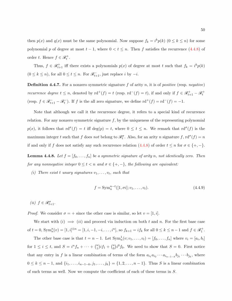
50

then p(x) and q(x) must be the same polynomial. Now suppose fk = ikp(k) (0 ≤ k ≤ n) for some

polynomial p of degree at most t − 1, where 0 < t ≤ n. Then f satisfies the recurrence (4.4.8) of

order t. Hence f ∈ R+t .

Thus, f ∈ R+t+1 iff there exists a polynomials p(x) of degree at most t such that fk = ikp(k)

(0 ≤ k ≤ n), for all 0 ≤ t ≤ n. For R−t+1, just replace i by −i.

Definition 4.4.7. For a nonzero symmetric signature f of arity n, it is of positive (resp. negative)

recurrence degree t ≤ n, denoted by rd+(f) = t (resp. rd−(f) = t), if and only if f ∈ R+t+1 −R+

t

(resp. f ∈ R−t+1 −R−t ). If f is the all zero signature, we define rd+(f) = rd−(f) = −1.

Note that although we call it the recurrence degree, it refers to a special kind of recurrence

relation. For any nonzero symmetric signature f , by the uniqueness of the representing polynomial

p(x), it follows that rdσ(f) = t iff deg(p) = t, where 0 ≤ t ≤ n. We remark that rdσ(f) is the

maximum integer t such that f does not belong to Rσt . Also, for an arity n signature f , rdσ(f) = n

if and only if f does not satisfy any such recurrence relation (4.4.8) of order t ≤ n for σ ∈ +,−.

Lemma 4.4.8. Let f = [f0, . . . , fn] be a symmetric signature of arity n, not identically zero. Then

for any nonnegative integer 0 ≤ t < n and σ ∈ +,−, the following are equivalent:

(i) There exist t unary signatures v1, . . . , vt, such that

f = Symn−tn ([1, σi]; v1, . . . , vt). (4.4.9)

(ii) f ∈ Rσt+1.

Proof. We consider σ = + since the other case is similar, so let v = [1, i].

We start with (i) =⇒ (ii) and proceed via induction on both t and n. For the first base case

of t = 0, Symnn(v) = [1, i]⊗n = [1, i,−1,−i, . . . , in], so fk+1 = ifk for all 0 ≤ k ≤ n− 1 and f ∈ R+

1 .

The other base case is that t = n − 1. Let Sym1n(v; v1, . . . , vt) = [f0, . . . , fn] where vi = [ai, bi]

for 1 ≤ i ≤ t, and S = infn + · · · +(n1

)if1 +

(n0

)i0f0. We need to show that S = 0. First notice

that any entry in f is a linear combination of terms of the form ai1ai2 · · · ain−1−kbj1 · · · bjk , where

0 ≤ k ≤ n − 1, and i1, . . . , in−1−k, j1, . . . , jk = 1, 2, . . . , n − 1. Thus S is a linear combination

of such terms as well. Now we compute the coefficient of each of these terms in S.

51

Each term ai1ai2 · · · ain−1−kbj1 · · · bjk appears twice in S, once in fk and the other time in fk+1.

In fk, the coefficient is k!(n−k)!, and in fk+1, it is i(k+ 1)!(n−k− 1)!. Thus, its coefficient in S is

(n

k + 1

)ik+1i(k + 1)!(n− k − 1)! +

(n

k

)ikk!(n− k)! = 0.

The above computation works for any such term due to the symmetry of f , so all coefficients in S

are 0, which means that S = 0.

Now assume for any t′ < t or for the same t and any n′ < n, the statement holds. For (n, t),

where n > t+1, assume that f = [f0, . . . , fn] = Symn−tn (v; v1, . . . , vt), g = Symn−t−1

n−1 (v; v1, . . . , vt) =

[g0, . . . , gn−1], and for any 1 ≤ j ≤ t, h(j) = Symn−tn−1(v; v1, . . . , vj−1, vj+1, . . . , vt) = [h

(j)0 , . . . , h

(j)n−1].

By the induction hypothesis, g satisfies the recurrence relation of order t + 1, namely g ∈ R+t+1.

Also for any j, h(j) satisfies the recurrence relation of order t, namely h(j) ∈ R+t ⊆ R+

t+1.

We have the recurrence relation

Symn−tn (v; v1, . . . , vt) = (n− t)v⊗Symn−t−1

n−1 (v; v1, . . . , vt) (4.4.10)

+t∑

j=1

vj⊗Symn−tn−1(v; v1, . . . , vj−1, vj+1, . . . , vt).

By (4.4.10), the entry of weight k in f for any k > 0 is

fk = (n− t)igk−1 +t∑

j=1

bjh(j)k−1.

We know that gi and h(j)i satisfy the recurrence relation (4.4.8) of order t + 1. Thus, their

linear combination fi also satisfies the recurrence relation (4.4.8) starting from i = k > 0.

We also observe that by (4.4.10), the entry of weight k in f for any k < n is

fk = (n− t)gk +t∑

j=1

ajh(j)k .

Since t < n − 1, by the same argument, the recurrence relation (4.4.8) holds for f when k = 0 as

well.

52

Now we show (ii) =⇒ (i). Notice that we only need to find unary signatures vi for 1 ≤ i ≤ t

such that Symn−tn (v; v1, . . . , vt) matches the first t+ 1 entries of f . The theorem follows from this

since we have shown that Symn−tn (v; v1, . . . , vt) satisfies the recurrence relation of order t + 1 and

any such signature is determined by the first t+ 1 entries.

We show that there exist vi = [ai, bi] (1 ≤ i ≤ t) satisfying the above requirement. Since f is not

identically zero, by (4.4.8), some nonzero term occurs among f0, . . . , ft. Let fs 6= 0, for 0 ≤ s ≤ t,

be the first nonzero term. By a nonzero constant multiplier, we may normalize fs = s!(n− s)!, and

set vj = [0, 1], for 1 ≤ j ≤ s (which is vacuous if s = 0), and set vs+j = [1, bs+j ], for 1 ≤ j ≤ t− s

(which is vacuous if s = t). Let F be the function defined in (4.4.9). Then Fk = fk = 0 for

0 ≤ k < s (which is vacuous if s = 0). By expanding the symmetrization function, for s ≤ k ≤ t,

we get

Fk = k!(n− k)!k−s∑j=0

(n− t

k − s− j

)∆ji

k−s−j ,

where ∆j is the elementary symmetric polynomial in bs+1, . . . , bt of degree j for 0 ≤ j ≤ t − s.

By definition, ∆0 = 1 and Fs = fs. Setting Fk = fk for s + 1 ≤ k ≤ t, this is a linear equation

system on ∆j (1 ≤ j ≤ t − s), with a triangular matrix and nonzero diagonals. From this, we

know that all ∆j ’s are uniquely determined by fs+1, . . . , ft. Moreover, bs+1, . . . , bt are the

roots of the equation∑t−s

j=0(−1)j∆jxt−j = 0. Thus bs+1, . . . , bt are also uniquely determined by

fs+1, . . . , ft up to a permutation.

Corollary 4.4.9. If f is a symmetric signature and σ ∈ +,−, then vdσ(f) + rdσ(f) = arity(f).

Thus we have an equivalent form of V σ for σ ∈ +,−. Namely,

V σ = f | 2 rdσ(f) < arity(f).

4.4.2 Characterizing Vanishing Signature Sets

Now we show that V + and V − capture all symmetric vanishing signature sets. To begin, we show

that a vanishing signature set cannot contain both types of nontrivial vanishing signatures.

53

Figure 4.2: Example of a gadget used to create a degenerate vanishing signature fromsome general vanishing signature. This example is for a signature of arity 7 and recur-rence degree 2, which is assigned to both vertices.

Lemma 4.4.10. Let f+ ∈ V + and f− ∈ V −. If neither f+ nor f− is the all zero signature, then

the signature set f+, f− is not vanishing.

Proof. Let arity(f+) = n and rd+(f+) = t, so 2t < n. Consider the gadget with two vertices

and 2t edges between two copies of f+. (See Figure 4.2 for an example of this gadget.) View

f+ in the symmetrized form. Since vd+(f+) = n − t, in each term, there are n − t many [1, i]’s

and t many unary signatures not equal to (a multiple of) [1, i]. This is a superposition of many

degenerate signatures. Then the only non-vanishing contributions come from the cases where the

n− 2t dangling edges on both sides are all assigned [1, i], while inside, the t copies of [1, i] pair up

with t unary signatures not equal to [1, i] from the other side perfectly. Notice that for any such

contribution, the Holant value of the inside part is always the same constant and this constant is

not 0 because [1, i] paired up with any unary signature other than (a multiple of) [1, i] is not 0.

Then the superposition of all of the permutations is a degenerate signature [1, i]⊗2(n−2t) up to a

nonzero constant factor.

Similarly, we can do this for f− of arity n′ and rd−(f−) = t′, where 2t′ < n′, and get a degenerate

signature [1,−i]⊗2(n′−2t′), up to a nonzero constant factor. Then form a bipartite signature grid

with (n′ − 2t′) vertices on one side, each assigned [1, i]⊗2(n−2t), and (n − 2t) vertices on the other

side, each assigned [1,−i]⊗2(n′−2t′). Connect edges between the two sides arbitrarily as long as it

is a 1-1 correspondence. The resulting Holant is a power of 2, which is not vanishing.

Lemma 4.4.11. Every symmetric vanishing signature is in V + ∪ V −.

Proof. Let f be a symmetric vanishing signature. We prove this by induction on n, the arity of f .

For n = 1, by connecting f = [f0, f1] to itself, we have f20 + f2

1 = 0. Then up to a constant factor,

we have either f = [1, i] or f = [1,−i]. The lemma holds.

54

For n = 2, first we do a self loop. The Holant is f0 +f2. Also, we can connect two copies of f , in

which case the Holant is f20 +2f2

1 +f22 . Since f is vanishing, both f0 +f2 = 0 and f2

0 +2f21 +f2

2 = 0.

Solving them, we get f = [1, i,−1] = [1, i]⊗2 or [1,−i,−1] = [1,−i]⊗2 up to a constant factor.

Now assume n > 2 and the lemma holds for any signature of arity k < n. Let f = [f0, f1, . . . , fn]

be a vanishing signature. A self loop on f gives f ′ = [f ′0, f′1, . . . , f

′n−2], where f ′j = fj + fj+2 for

0 ≤ j ≤ n − 2. Since f is vanishing, f ′ is vanishing as well. By the induction hypothesis,

f ′ ∈ V + ∪ V −.

If f ′ is an all zero signature, then we have fj + fj+2 = 0 for 0 ≤ j ≤ n− 2. This means that the

fj ’s satisfy a recurrence relation with characteristic polynomial x2 +1, so we have fj = aij + b(−i)j

for some a and b. Then we perform a holographic transformation with Z = 1√2

[1 1i −i

],

Holant(=2 | f) ≡T Holant([1, 0, 1]Z⊗2 | (Z−1)⊗nf)

≡T Holant([0, 1, 0] | f),

where f = [a, 0, . . . , 0, b]. The problem Holant([0, 1, 0] | f) is a weighted version of testing if a graph

is bipartite. Now consider a graph with only two vertices, both assigned f , and n edges between

them. The Holant of this graph is 2ab. However, we know that it must be vanishing, so ab = 0. If

a = 0, then f ∈ V −. Otherwise, b = 0 and f ∈ V +.

Now suppose that f ′ is in V + ∪V − but is not an all zero signature. We consider f ′ ∈ V + since

the other case is similar. Then rd+(f ′) = t, so 2t < n− 2. Consider the gadget which has only two

vertices, both assigned f ′, and has 2t edges between them. (See Figure 4.2 for an example of this

gadget.) It forms a signature of degree d = 2(n− 2− 2t). This gadget is valid because n− 2 > 2t.

By the combinatorial view as in the proof of Lemma 4.4.10, this signature is [1, i]⊗d.

Moreover, rd+(f ′) = t implies that the entries of f ′ satisfy a recurrence of order t+1. Replacing

f ′j by fj + fj+2, we get a recurrence relation for the entries of f with characteristic polynomial

(x2 +1)(x− i)t+1 = (x+ i)(x− i)t+2. Thus, fj = ijp(j)+ c(−i)j for some polynomial p(x) of degree

at most t+ 1 and some constant c. It suffices to show that c = 0 since 2(t+ 1) < n as 2t < n− 2.

Consider the signature h = [h0, . . . , hn−1] created by connecting f with a single unary signature

55

[1, i]. For any (n − 1)-regular graph G = (V,E) with h assigned to every vertex, we can define a

duplicate graph of (d+ 1)|V | vertices as follows. First for each v ∈ V , define vertices v′, v1, . . . , vd.

For each i, 1 ≤ i ≤ d, we make a copy of G on vi | v ∈ V , i.e., for each edge (u, v) ∈ E, include

the edge (ui, vi) in the new graph. Next for each v ∈ V , we introduce edges between v′ and vi for

all 1 ≤ i ≤ d. For each v ∈ V , assign the degenerate signature [1, i]⊗d that we just constructed to

the vertices v′; assign f to all the vertices v1, . . . , vd. Assume the Holant of the original graph G

with h assigned to every vertex is H. Then for the new graph with the given signature assignments,

the Holant is Hd. By our assumption, f is vanishing, so Hd = 0. Thus, H = 0. This holds for any

graph G, so h is vanishing.

Notice that hk = fk+ifk+1 for any 0 ≤ k ≤ n−1. If h is identically zero, then fk+ifk+1 = 0 for

any 0 ≤ k ≤ n− 1, which means f = [1, i]⊗n up to a constant factor and we are done. Otherwise,

suppose that h is not identically zero. By the inductive hypothesis, h ∈ V + ∪ V −. We claim h

cannot be from V −. This is because, although we do not directly construct h from f , we can always

realize it by the method depicted in the previous paragraph. Therefore the set f ′, h is vanishing.

As both f ′ and h are nonzero, and f ′ ∈ V +, we have h 6∈ V −, by Lemma 4.4.10.

Hence h is in V +. Then there exists a polynomial q(x) of degree at most t′ =⌊n−1

2

⌋such

that hk = ikq(k), for any 0 ≤ k ≤ n − 1. Since 2t < n − 2, we have t ≤ t′. On the other hand,

hk = fk + ifk+1 for any 0 ≤ k ≤ n− 1, so we have

hk = fk + ifk+1

= ikp(k) + c(−i)k + i(ik+1p(k + 1) + c(−i)k+1

)= ik (p(k)− p(k + 1)) + 2c(−i)k

= ikr(k) + 2c(−i)k

= ikq(k),

where r(x) = p(x)− p(x+ 1) is another polynomial of degree at most t. Then we have

q(k)− r(k) = 2c(−1)k,

56

which holds for all 0 ≤ k ≤ n−1. Notice that the left hand side is a polynomial of degree at most t′,

call it s(x). However, for all even k ∈ 0, . . . , n−1, s(k) = 2c. There are exactly⌈n2

⌉>⌊n−1

2

⌋= t′

many even k within the range 0, . . . , n − 1. Thus s(x) = 2c for any x. Now we pick k = 1, so

s(1) = −2c = 2c, which implies c = 0. This completes the proof.

Combining Lemma 4.4.5, Lemma 4.4.10, and Lemma 4.4.11, we obtain the following theorem

that characterizes all symmetric vanishing signature sets.

Theorem 4.4.12. Let F be a set of symmetric signatures. Then F is vanishing if and only if

F ⊆ V + or F ⊆ V −.

To finish this subsection, we prove some useful properties regarding vanishing and recurrence

degrees in the construction of signatures. For two symmetric signatures f and g such that arity(f) ≥

arity(g), let 〈f, g〉 = 〈g, f〉 denote the signature that results after connecting all edges of g to f . (If

arity(f) = arity(g), then 〈f, g〉 is a constant, which can be viewed as a signature of arity 0.)

Lemma 4.4.13. For σ ∈ +,−, suppose symmetric signatures f and g satisfy vdσ(g) = 0 and

arity(f)− arity(g) ≥ rdσ(f). Then rdσ(〈f, g〉) = rdσ(f).

Proof. We consider σ = + since the case σ = − is similar. Let arity(f) = n, arity(g) = m, and

rd+(f) = t. Denote the signature 〈f, g〉 by f ′.

If t = −1, then f is identically zero and so is f ′. Hence rd+(f ′) = −1.

Suppose t ≥ 0. Then we have fk = ikp(k) where p(x) is a polynomial of degree exactly t. Also

arity(f ′) = n−m ≥ t. We have

f ′k =

m∑j=0

(m

j

)fk+jgj

= ikm∑j=0

(m

j

)p(k + j)ijgj

= ikq(k),

where q(k) =∑m

j=0

(mj

)p(k+j)ijgj is a polynomial in k. Notice that vd+(g) = 0. Then rd+(g) = m

and g 6∈ R+m. Thus

∑mj=0

(mj

)ijgj 6= 0. Then the leading coefficient of degree t in the polynomial

57

q(k) is nonzero. However, arity(f ′) ≥ t. Thus rd+(f ′) = t as well.

Lemma 4.4.14. For σ ∈ +,−, let f be a nonzero symmetric signature and suppose that f ′ is

obtained from f by a self loop. If vdσ(f) > 0, then vdσ(f)− vdσ(f ′) = rdσ(f)− rdσ(f ′) = 1.

Proof. We may assume σ = +, arity(f) = n, and rd+(f) = t. Since f is not the all zero signature,

t ≥ 0. Also since vd+(f) > 0, t = n − vd+(f) < n. By assumption, we have fk = ikp(k), where

p(x) is a polynomial of degree exactly t. Then we have

f ′k = fk + fk+2

= ik(p(k)− p(k + 2))

= ikq(k),

where q(k) = p(k) − p(k + 2) is a polynomial in k. If t = 0, then p(x) is a constant polynomial

and q(x) is identically zero. Then rd+(f ′) = −1 by definition and rd+(f) − rd+(f ′) = 1 holds.

Suppose t > 0, then in q(k), the term of degree t has a zero coefficient, but the term of degree t− 1

is nonzero. So q(x) has degree exactly t− 1 ≤ n− 2 = arity(f ′). Thus rd+(f ′) = t− 1. Notice that

arity(f)− arity(f ′) = 2, then vd+(f)− vd+(f ′) = 1 as well.

Moreover, the set of vanishing signatures is closed under orthogonal transformations. This

is because under any orthogonal transformation, the unary signatures [1, i] and [1,−i] are either

invariant or transformed into each other. Then considering the symmetrized form of any signature,

we have the following lemma.

Lemma 4.4.15. For a symmetric signature f of arity n, σ ∈ +,−, and an orthogonal matrix

T ∈ C2×2, either vdσ(f) = vdσ(T⊗nf) or vdσ(f) = vd−σ(T⊗nf).

58

4.4.3 Characterizing Vanishing Signatures via a Holographic Transformation

There is another explanation for the vanishing signatures. Given an f ∈ V + with arity(f) = n and

rd+(f) = d, we perform a holographic transformation with Z = 1√2

[1 1i −i

],

Holant(=2 | f) ≡T Holant([1, 0, 1]Z⊗2 | (Z−1)⊗nf)

≡T Holant([0, 1, 0] | f),

where f is of the form [f0, f1, . . . , fd, 0, . . . , 0], and fd 6= 0. To see this, note that Z−1 = 1√2

[1 −i1 i

]and Z−1 [ 1

i ] =√

2 [ 10 ]. We know that f has a symmetrized form, such as Symn−d

n ([ 1i ] ; v1, . . . , vd).

Then up to a factor of 2n/2, we have f = (Z−1)⊗nf = Symn−dn ([ 1

0 ] ;u1, . . . , ud), where ui = Z−1vi

for 1 ≤ i ≤ d and ui and vi are column vectors in C2. From this expression for f , it is clear

that all entries of Hamming weight greater than d in f are 0. Moreover, if fd = 0, then one

of the ui has to be a multiple of [1, 0]. This contradicts the degree assumption of f , namely

vd+(f) = n− rd+(f) = n− d and no higher.

From this discussion, we have the following lemma.

Lemma 4.4.16. Suppose f is a symmetric signature of arity n. Let f = (Z−1)⊗nf . If rd+(f) = d,

then f = [f0, f1, . . . , fd, 0, . . . , 0] and fd 6= 0. Also f ∈ R+d iff all nonzero entries of f are among

the first d entries in its symmetric signature notation.

Similarly, if rd−(f) = d, then f = [0, . . . , 0, fn−d, . . . , fn] and fn−d 6= 0. Also f ∈ R−d iff all

nonzero entries of f are among the last d entries in its symmetric signature notation.

This presentation of vanishing signatures follows the order in which we thought about them.

Initially, we viewed them as summations of degenerate signatures with more than have [1, i]’s or

[1,−i]’s. For this reason, we defined the notions of positive and negative vanishing degrees to

indicate how many [1, i]’s or [1,−i]’s respectively can exist in such an expression. Next we realized

that the entries of a symmetric vanishing signature satisfy a recurrence relation involving ±i. For

this reason, we defined the notions of positive and negative recurrence degrees to indicate the order

of this recurrence relation. Lastly, we gained the perspective of vanishing signatures in the Z basis

as described above.

59

In any bipartite graph for Holant([0, 1, 0] | f), the binary Disequality (6=2) = [0, 1, 0] on the

left imposes the condition that half of the edges must take the value 0 and the other half must

take the value 1. On the right side, by f ∈ V +, we have d < n/2, thus f requires that less than

half of the edges are assigned the value 1. Therefore the Holant is always 0. A similar conclusion

was reached in [50] for certain (2, 3)-regular bipartite Holant problems with Boolean signatures.

However, the importance was not realized at that time—not until the spring of 2012. At that time,

we were working on [30], and Jin-Yi Cai was teaching a special topics course called Complexity

of Counting Problems in which he presented [50]. When he stated that some cases were tractable

because their Holant is always 0, Heng Guo immediately did the calculations to verify the vanishing

and recurrence degrees of the signatures involved when expressed in the standard basis.

I now believe that this Z-basis view is the right way to think about vanishing signatures. Not

only is the argument that they are vanishing trivial, but it is also a useful generalization to signatures

that are not symmetric. In contrast, definition of vanishing signatures using the vanishing degrees is

not that helpful, and it is not clear how to generalize recurrence degrees to asymmetric signatures.

Furthermore, gadget constructions with vanishing signatures in the Z basis are more combinatorial,

easier to find, and easier to explain than the same gadget constructions in the standard basis.

Open Problem 4.4.17. Are there any complex-weighted signatures over the Boolean domain that

are vanishing for some reason other than the one provided by the Z-basis view?

In our characterization of symmetric vanishing signatures, one can check that all of our gadget

constructions are planar. This means that there does not exist a signature that is vanishing over

planar graphs but is not vanishing over general graphs. This makes me think of the following

question.

Open Problem 4.4.18. Does there exists an “interesting” class C of graphs and a signature f

such that f is vanishing over C but not vanishing over general graphs?

Although vanishing signatures were first introduced in [72] in the parity setting (where a signa-

ture set is vanishing if the corresponding Holant value is always 0 modulo 2), a complete charac-

terization of those vanishing signatures was not given. Thus, the dichotomy in [72] is not currently

60

known to be decidable. The difficulty in the parity setting is that each vanishing signature over

the Gaussian integers corresponds to a vanishing signature over Z2. Since 12 ≡ −1 (mod 2), the

element 1 is a square root of 1 over Z2 just like i is a square root of 1 over C. Therefore, a vanishing

signature f over the Gaussian integers corresponds to a vanishing signature over Z2 by mapping

any occurrence of i to 1 and then reducing modulo 2. Given our characterization for vanishing

signatures over C and the partial characterization of vanishing signatures over Z2 in [72], I expect

that one can now obtain a complete characterization the vanishing signatures over Z2, thereby

making the dichotomy in [72] decidable.

61

Chapter 5

Dichotomy for #H-Coloring Problems

over Planar 3-Regular Directed

Graphs

In this chapter, we introduce an idea called anti-gadgets in complexity reductions. These combi-

natorial gadgets have the effect of erasing the presence of some other graph fragment, as if we had

managed to include a negative copy of a graph gadget. We use this idea to prove a dichotomy for a

generalization of counting graph homomorphisms that allows for complex weights. This work was

published in [38, 39].

5.1 Background

Reduction, the method of transforming one problem to another, and thereby proving the hardness

of a problem for an entire complexity class, is arguably the most successful tool in complexity

theory to date. When expressed in terms of graph problems, a typical reduction from problem

Π1 to problem Π2 is carried out by designing a gadget—a graph fragment with some desirable

properties. The reduction starts from an instance graph G1 for Π1 and introduces one or more

copies of the gadget to obtain an instance graph G2 (or possibly multiple instance graphs) for Π2.

62

The graph G2 may contain a polynomial number of copies of the gadget. But can it include

some negative copies of a gadget? Of course not; the notion of a negative graph fragment seems

meaningless. However, we introduce an idea in reduction theory that has the effect of introducing

negative copies of a gadget in a reduction. More precisely, we show that our new construction

idea, when expressed in algebraic terms, has the same effect as erasing the presence of some graph

fragment. It is as if we managed to include a negative copy of a certain gadget. We call this

an anti-gadget. It is analogous to the pairing of a particle and its anti-particle in physics. We

demonstrate the elegance and usefulness of anti-gadgets by proving a new complexity dichotomy

theorem in counting complexity where anti-gadgets play a decisive role. Furthermore, we show that

anti-gadgets provide a simple explanation for some miraculous cancellations that were observed in

previous results [37, 36]. We also observe how anti-gadgets can guide the search for such gadget

sets more by design than by chance.

The new dichotomy theorem that we prove using anti-gadgets can be stated in terms of spin

systems over 3-regular graphs with vertices taking values in 0, 1 and an arbitrary complex-valued

edge function f(·, ·) = (w, x, y, z) that is not necessarily symmetric. Define the partition function

on G = (V,E) as

Z(G) =∑

σ:V (G)→0,1

∏(u,v)∈E(G)

f(σ(u), σ(v)).

Depending on the nature of the edge function f , we show that the problem Z(·) is either com-

putable in polynomial time or #P-hard. The tractable cases were what we expected: (1) product-

type signatures, (2) holographic reductions to affine signatures, and (3) holographic reductions to

matchgate signatures with the input restricted to planar graphs. The formal statement is given in

Theorem 5.4.1. This dichotomy extends several previous ones that considered a symmetric edge

function [50, 48, 93].

This partition function Z(G) computes the sum of weighted graph homomorphisms from the

input graph G to the 2-vertex target graph H with weighted adjacency matrix [w xy z ]. It is also

known as the #H-coloring problem. Recall from Lemma 2.3.1 that we can express this problem

as a counting Constraint Satisfaction Problem (#CSP). Then by Lemma 2.2.1, we can further

express this problem as a Holant problem. Compared to #CSP and graph homomorphisms, the

63

(a) As a bipartite (2,3)-regular graph (b) As a 3-regular directed graph

Figure 5.1: The two representations of an (f | =3)-gate.

main difficulty here is bounded degree, which makes hardness proofs more challenging, and for a

good reason—there are indeed more tractable cases.

We give a directed explanation of how to express Z(·) as a Holant problem (which is really

the combined proofs of Lemma 2.3.1 and Lemma 2.2.1 that are simplified for this specific case).

Given any 3-regular directed graph G = (V,E), its edge-vertex incidence graph G′ has vertex set

V (G′) = V ∪ E and edge set E(G′) = (v, e) | v is incident to e in G. The graph G′ is bipartite

and (2, 3)-regular. To each v ∈ V ⊂ V (G′), we assign the Equality function =3 of arity 3. To

each e ∈ E ⊂ V (G′), we assign the original edge function f from G. Furthermore, we assign the

first (resp. second) input of f to the edge incident to the vertex in V that is incident to the tail

(resp. head) of the directed edge in G. Then the Holant value on G′ is exactly the partition function

Z(G). Essentially =3 forces all incident edges in G′ at a vertex v ∈ V ⊂ V (G′) to take the same

value, which reduces to vertex assignments on V , as in Z(G).

As a Holant problem (over (2, 3)-regular bipartite graphs), this partition function is expressed

as Holant(f | =3), where f = (w, x, y, z). Our main result is a dichotomy theorem for this problem,

where w, x, y, z ∈ C. To describe an (f | =3)-gate though, it is simpler to depict it as a fragment of

a 3-regular directed graph. Figure 5.1 gives an example of an (f | =3)-gate both as a (2, 3)-regular

(a) (b)

. . . . . .

(c)

Figure 5.2: An arity 4-to-1 projective gadget (a), a recursive gadget (b), and a planarembedding of their interpolation construction (c). My wife thinks (c) looks like a pencil;I agree.

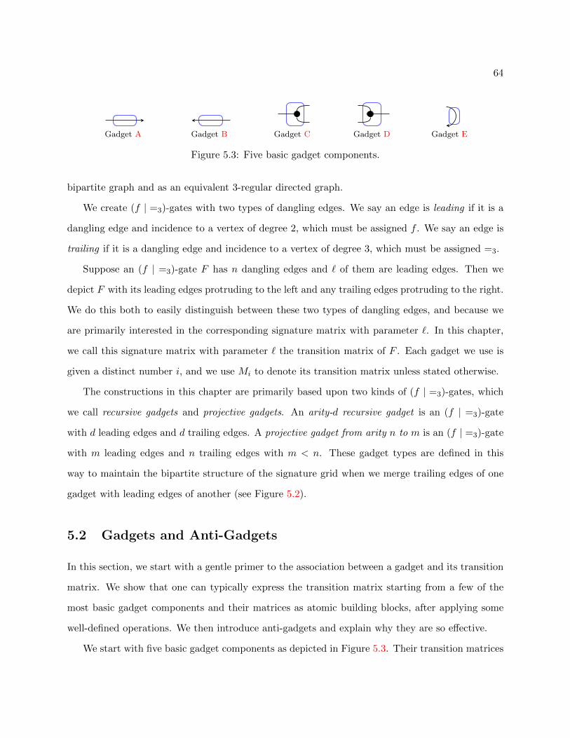
64

Gadget A Gadget B Gadget C Gadget D Gadget E

Figure 5.3: Five basic gadget components.

bipartite graph and as an equivalent 3-regular directed graph.

We create (f | =3)-gates with two types of dangling edges. We say an edge is leading if it is a

dangling edge and incidence to a vertex of degree 2, which must be assigned f . We say an edge is

trailing if it is a dangling edge and incidence to a vertex of degree 3, which must be assigned =3.

Suppose an (f | =3)-gate F has n dangling edges and ` of them are leading edges. Then we

depict F with its leading edges protruding to the left and any trailing edges protruding to the right.

We do this both to easily distinguish between these two types of dangling edges, and because we

are primarily interested in the corresponding signature matrix with parameter `. In this chapter,

we call this signature matrix with parameter ` the transition matrix of F . Each gadget we use is

given a distinct number i, and we use Mi to denote its transition matrix unless stated otherwise.

The constructions in this chapter are primarily based upon two kinds of (f | =3)-gates, which

we call recursive gadgets and projective gadgets. An arity-d recursive gadget is an (f | =3)-gate

with d leading edges and d trailing edges. A projective gadget from arity n to m is an (f | =3)-gate

with m leading edges and n trailing edges with m < n. These gadget types are defined in this

way to maintain the bipartite structure of the signature grid when we merge trailing edges of one

gadget with leading edges of another (see Figure 5.2).

5.2 Gadgets and Anti-Gadgets

In this section, we start with a gentle primer to the association between a gadget and its transition

matrix. We show that one can typically express the transition matrix starting from a few of the

most basic gadget components and their matrices as atomic building blocks, after applying some

well-defined operations. We then introduce anti-gadgets and explain why they are so effective.

We start with five basic gadget components as depicted in Figure 5.3. Their transition matrices

65

are A = [w xy z ], B = [w y

x z ], C = [ 1 0 0 00 0 0 1 ], D =

[1 00 00 00 1

], and E =

[wxyz

].

The first operation is matrix product, which corresponds to sequentially connecting two gadgets

together. For example, Gadget 1 is a simple composition of Gadget B and Gadget C, and thus its

transition matrix is the matrix product BC =[w 0 0 yx 0 0 z

](see Figure 5.5a). The second operation

is tensor product, which corresponds to putting two gadgets in parallel (two disconnected parts).

The transition matrix of Gadget 2 is ACB⊗2D =[

w3+x3 wy2+xz2

w2y+x2z y3+z3

], where B⊗2 corresponds to the

parallel part of the gadget and is clearly visible in Figure 5.5b. Similarly, Gadget 3 has transition

matrix AC(A⊗B)D. Note that the order of the tensor product is to make the top leading edge for

the row (resp. the top trailing edge for the column) the most significant bit. The transition matrices

of Gadget 4 and Gadget 5 are respectively [w xy z ]⊗2 diag(w, x, y, z) and [w x

y z ]⊗2 diag(w, y, x, z) and

can be mechanically derived by our gadgetry calculus as A⊗2(C ⊗ I2)(I2 ⊗ A ⊗ I2)(I2 ⊗ D) and

A⊗2(C ⊗ I2)(I2 ⊗ B ⊗ I2)(I2 ⊗ D). The composition of Gadget 4 is illustrated in Figure 5.5c.

Gadget E is used to create a self-loop, as in Gadget 6, which has transition matrix AC(A⊗ I2)(C⊗

I2)(BCE ⊗ I4)(A⊗B)D. The composition of Gadget E is illustrated in Figure 5.5c.

Now we introduce a powerful new technique called anti-gadgets.

Definition 5.2.1. Let G be a recursive gadget with transition matrix M . Then a recursive gadget

G′ is called an anti-gadget of G if the transition matrix of G′ is λM−1, for some λ ∈ C− 0.

A crucial ingredient in our proof of #P-hardness is to produce an arbitrarily large set of pairwise

linearly independent signatures. These signatures are used to form a Vandermonde system of full

rank. One common way to produce an arbitrarily large set of signatures is to compose copies of a

recursive gadget. Let M be the transition matrix of some recursive gadget G. Composing k copies

of G produces a gadget with transition matrix Mk. If M has infinite order (up to a scalar), then

Gadget 1 Gadget 2 Gadget 3 Gadget 4 Gadget 5 Gadget 6

Figure 5.4: Recursive and projective gadgets.

66

(a) Composition of Gadget 1 (b) Composition of Gadget 2 (c) Composition of Gadget 4

(d) Composition of Gadget 6

Figure 5.5: Gadget compositions using the basic gadget components in Figure 5.3.

we have an arbitrarily large set of pairwise linearly independent signatures. Now suppose that M

has finite order (up to a scalar), that is, for some positive integer k, Mk = λI, a nonzero multiple

of the identity matrix. Then composing only k− 1 copies of G results in a gadget with a transition

matrix that is the inverse of G’s transition matrix (up to a scalar). This is an anti-gadget of G.

If an anti-gadget of G is composed with another gadget containing similar structure to that of

G, then cancellations ensue and the composition yields a transition matrix that can be quite easy to

analyze. E.g., Gadget 4 and Gadget 5 only differ by the orientation of the vertical edge. When com-

posing an anti-gadget of Gadget 4 with Gadget 5, the contribution of the two leading edges cancel

and we get M−14 M5 = diag(w, x, y, z)−1

([w xy z ]⊗2

)−1[w xy z ]⊗2 diag(w, y, x, z) = diag(1, y/x, x/y, 1).

The resulting transition matrix has infinite order unless x/y is a root of unity. This situation is

analyzed formally in Lemma 5.5.1.

Another use of the anti-gadget technique can be applied with Gadget 2 and Gadget 3. Once

again, the contribution of the leading edge cancels when composing an anti-gadget of Gadget 3

with Gadget 2. The resulting matrix is a bit more complicated this time. However, when this pair

of gadgets is analyzed formally in Lemma 5.5.2, the assumptions are x = 0∧wyz 6= 0. In that case,

M−13 M2 =

[1 y2/w2

0 1

]. This matrix clearly has infinite order (up to a scalar).

5.3 Interpolation Techniques

The method of polynomial interpolation has been pioneered by Valiant [126] and further developed

by many others [59, 124, 14, 17, 50]. In this section, we give a new unified technique to interpolate

67

all unary signatures. This is our main technical step to prove #P-hardness. Our method produces

an infinite set of pairwise linearly independent vectors at any fixed dimension, and then projects

to a lower dimension while retaining pairwise linear independence of a nontrivial fraction.

In previous work, “finisher gadgets” [93, 37, 36] were used to handle the symmetric case, map-

ping symmetric arity 2 signatures to arity 1 signatures. In our language, a finisher gadget is a

projective gadget from a projective gadget from arity 2 to 1.

In this chapter, we introduce projective gadget sets. These gadget sets are completely general,

in the sense that they can be used to map any set of pairwise linearly independent signatures

(symmetric or asymmetric) to any lower arity, while preserving pairwise linear independence for

an inverse polynomial fraction. This permits much more freedom in gadget constructions, and this

power is used crucially in the proof of our dichotomy theorem. This advance is not just a simple

matter of searching for the right gadgets. One must find the abstract criteria for success that can

be simultaneously satisfied by gadgets that exist in practice. These developments, together with

the anti-gadget concept, come together in the Group Lemma, which provides a straightforward

criterion for proving #P-hardness of certain Holant problems.

Definition 5.3.1. A set of matrices M ⊆ C2m×2n forms a projective set from arity n to m if for

any matrix N ∈ C2n×2 with rank 2, there exists a matrix M ∈M such that MN has rank 2.

We also call a set of gadgets projective from arity n to m if the set of its signature matrices is

projective from arity n to m. A (G | R)-gate set that is projective from arity 2-to-1 can be used to

transform a pair of (G | R)-gates with linearly independent binary signatures to a pair of (G | R)-

gates with linearly independent unary signatures. Projective gadgets in such a set have two trailing

edges and one leading edge, but can also be viewed as operating on signatures of higher arity, with

the identity transformation being performed on the other edges not connected to the projective

gadget. This way of connecting the projective gadget to an existing (G | R)-gate automatically

gives us projective gadget sets for higher arities. But first, a quick lemma to assist with the proof.

Lemma 5.3.2. Let v0 and v1 be nonzero column vectors, not necessarily the same length. Then

the block matrix[av0 bv0cv1 dv1

]has rank 2 if and only if

[a bc d

]is invertible.

68

Proof. We write[av0 bv0cv1 dv1

]=[v0 00 v1

][ a bc d], and

[v0 00 v1

]has rank 2. Thus

[av0 bv0cv1 dv1

]has rank 2 if and

only if[a bc d

]is invertible.

Lemma 5.3.3. Let G and R be signature sets. Suppose P is a projective (G | R)-gate set from

arity 2-to-1. Then for all integers k ≥ 2, P acts as a projective (G | R)-gate set from arity k to

k − 1.

Proof. We are given that for any N ∈ C4×2 with rank 2, there exists an F ∈ P with F ∈ C2×4

such that FN is invertible. We want to show that for any integer k ≥ 2 and any rank 2 matrix

B ∈ C2k×2, there exists an F ∈ P such that (I ⊗ F )B has rank 2, where I is the 2k−2-by-2k−2

identity matrix.

For any F ∈ P, the matrix I ⊗ F can be viewed as being composed of 2-by-4 blocks, with F

appearing along the main diagonal and 2-by-4 zero-matrices elsewhere. We similarly view B as

being composed of 4-by-2 blocks B =

B1B2

...B

2k−2

. Then (I ⊗ F )B =

FB1FB2

...FB

2k−2

∈ C2k−1×2. If some

Bi has rank 2, then there is an F ∈ P such that FBi is invertible and (I ⊗ F )B has rank 2, as

desired.

Now assume otherwise, so each Bi has rank at most 1. Since B has rank 2, there exists a

2-by-2 invertible submatrix D of B, for which the rows of D appear in Bi and Bj , for some i < j.

It follows that Bi and Bj both have rank exactly 1. Hence for some nonzero vectors v0, v1 ∈ C4

and some a, b, c, d ∈ C, we can write Bi = [av0 bv0] and Bj = [cv1 dv1]. By Lemma 5.3.2,[a bc d

]is invertible, as

[BiBj

]has rank 2. If v0 and v1 are linearly independent, then choose F ∈ P such

that F [v0 v1] is invertible; otherwise let v ∈ C4 be such that v0 and v are linearly independent,

and choose F ∈ P such that F [v0 v] is invertible. In either case (ignoring v in the second case),

we define [v′0 v′1] = F [v0 v1], where v′0 and v′1 are nonzero. Then by Lemma 5.3.2, the matrix[av′0 bv

′0

cv′1 dv′1

]=[FBiFBj

]has rank 2, and since this appears as a submatrix of (I⊗F )B, we are done.

Corollary 5.3.4. Let G and R be signature sets. Suppose P is a finite projective (G | R)-gate set

from arity 2-to-1. Then for any integer k ≥ 2, P induces a finite projective (G | R)-gate set from

arity k to 1.

69

Now we show that a finite projective (G | R)-gadget set from arity k to 1 preserves pairwise

linear independence for an inverse polynomial fraction of signatures. The essence of the next lemma

is an exchange in the order of quantifiers.

Lemma 5.3.5. Suppose vii≥0 is a sequence of pairwise linearly independent column vectors in

C2k and let F ⊆ C2×2k be a finite set of f matrices that is projective from arity k to 1. Then for

every n, there exists some F ∈ F and some S ⊆ Fvi | 0 ≤ i ≤ nf such that |S| ≥ n and the

vectors in S are pairwise linearly independent.

Proof. Let j > i ≥ 0 be integers and let N = [vi vj ] ∈ C2k×2. Since vi and vj are linearly

independent, rank(N) = 2. By assumption, there exists an F ∈ F such that FN ∈ C2×2 is

invertible, so we conclude that Fvi and Fvj are linearly independent.

Each F ∈ F defines a coloring of the set K = 0, 1, . . . , nf as follows: color i ∈ K with

the linear subspace spanned by Fvi. Assume for a contradiction that for each F ∈ F , there is

not n pairwise linearly independent vectors among Fvi | i ∈ K. Then, including possibly the

0-dimensional subspace 0, there can be at most n distinct colors assigned by each F ∈ F . By the

pigeonhole principle, some i and j with 0 ≤ i < j ≤ nf must receive the same color for all F ∈ F .

This is a contradiction with the previous paragraph, so we are done.

The next lemma says that under suitable conditions, we can construct all unary signatures

(X,Y ). The method will be interpolation at a higher dimensional iteration in a circular fashion

and finishing with an appropriate projective gadget.

Lemma 5.3.6 (Group Lemma). For signature sets G and R, suppose there exists a finite set of

projective (G | R)-gates from arity 2-to-1, and suppose S is a finite set of recursive (G | R)-gates

of arity d ≥ 1 with nonsingular transition matrices. Let H be the group generated by the transition

matrices of gadgets in S, modulo scalar matrices λI, for λ ∈ C−0. If H has infinite order, then

Holant(G ∪ (X,Y ) | R) ≤T Holant(G | R)

for any X,Y ∈ C.

70

Proof. Two matrices are unequal modulo scalar matrices λI if and only if they are linearly inde-

pendent. If any member of S, as a group element in H, has infinite order, then its powers supply

an infinite set of pairwise linearly independent signatures. Otherwise they all have finite order, and

the group H is identical to the monoid generated by S, i.e., every h ∈ H is a product over S with

non-negative powers. Such products give a composition of gadgets in S, which is a recursive gadget.

By assumption, H has infinite order, so by composing recursive gadgets from S, a breadth-first

traversal of the Cayley graph of the monoid generated by S supplies an arbitrarily large set of

recursive gadgets having pairwise linearly independent signatures.

Before we can use a projective gadget set to project the set of pairwise linearly independent

signatures down to arity 1, we make a small modification to each corresponding gadget: connect

a non-degenerate signature g ∈ G to every trailing edge. This ensures that the bipartite structure

of the graph is preserved when applying projective gadgets. We claim that there is some non-

degenerate signature g ∈ G. If this were not the case, then any recursive gadget s ∈ S (note S is

nonempty) could be rewritten with all leading edges internally incident to unary signatures. The

recurrence matrix of such a gadget is expressible as a product of a column vector and a row vector

(by partitioning s into two gadgets with no shared edges), hence the recurrence matrix of s would

have rank at most 1, which is less than 2d as promised. Let a ≥ 2 be the arity of g. One can show

by induction that any non-degenerate signature has at least one index i, such that if we express

the signature as a 2-by-2a−1 matrix M indexed by the i-th variable for the row and the remaining

a − 1 variables for the column, then M has rank 2. We designate one such dangling edge of g as

the leading edge and all other dangling edges as trailing edges. As there are d trailing edges in s,

we apply d copies of g, which corresponds to multiplication by the matrix M⊗d. Since M has full

rank, pairwise linear independence of the signatures is preserved. Now rewrite the 2d-by-2d(a−1)

matrix form of the signature as a column vector in C2da , indexed by cd(a−1) · · · c1b1 · · · bd ∈ 0, 1da,

where b1 · · · bd and c1 · · · cd(a−1) are the row and column indices. Denote these vectors as vii≥0.

Finally we can attach projective gadgets to project each vi down to arity 1. (see Figure 5.2c).

To show Holant(G ∪ (X,Y ) | R) ≤T Holant(G | R), suppose we are given as input a bipartite

signature grid Ω for Holant(G ∪ (X,Y ) | R), with underlying graph G = (V,E). Let Q ⊆ V be

71

the set of vertices labeled with (X,Y ), and let n = |Q|. By Corollary 5.3.4, there exists a finite

projective set containing f gadgets from arity d to 1, so by Lemma 5.3.5, there is some projective

gadget F in this set such that at least n + 2 of the first (n + 2)f + 1 vectors of the form Fvt

are pairwise linearly independent. It is straightforward to efficiently find such a set; denote it by

S = (X0, Y0), (X1, Y1), . . . , (Xn+1, Yn+1), and let G0, G1, . . . , Gn+1 be the corresponding gadgets.

At most one Yt can be zero, so without loss of generality, assume Yt 6= 0 for 0 ≤ t ≤ n. If we

replace every element of Q with a copy of Gt, we obtain an instance of Holant(G | R) (note that the

correct bipartite structure is preserved), and we denote this new signature grid by Ωt. Although

Holant(Ωt) is a sum of exponentially many terms, each nonzero term has the form bXitY

n−it for

some i and for some b ∈ C that does not depend on Xt or Yt. Then for some c0, c1, . . . , cn ∈ C, the

sum can be rewritten as

Holant(Ωt) =∑

0≤i≤nciX

itY

n−it .

Since each signature grid Ωt is an instance of Holant(G | R), Holant(Ωt) can be solved exactly using

the oracle. Carrying out this process for every t where 0 ≤ t ≤ n, we arrive at a linear system

where the ci values are the unknowns.

Y −n0 ·Holant(Ω0)

Y −n1 ·Holant(Ω1)

...

Y −nn ·Holant(Ωn)

=

X00Y

00 X1

0Y−1

0 · · · Xn0 Y−n

0

X01Y

01 X1

1Y−1

1 · · · Xn1 Y−n

1

......

. . ....

X0nY

0n X1

nY−1n · · · Xn

nY−nn

c0

c1

...

cn

The matrix above has entry (Xr/Yr)

c at row r and column c. Due to pairwise linear independence

of (Xr, Yr), we have that Xr/Yr is pairwise distinct for 0 ≤ r ≤ n. Hence this is a Vandermonde

system of full rank, and we can solve it for the ci values. With these values in hand, we can calculate

Holant(Ω) =∑

0≤i≤nciX

iY n−i,

completing the reduction.

72

Remark. Every time we apply Lemma 5.3.6, we do so in the simpler case that H contains an

element of infinite order. We had initially hoped to find a useful failure condition from group

theory when H has finite order, but we did not find such a condition.

Here is how we realize a projective set of gadgets from arity 2-to-1.

Lemma 5.3.7. Let Φi ∈ C2×4 for 1 ≤ i ≤ 7 be matrices with the following properties: ker(Φi) =

spanu, ui for 1 ≤ i ≤ 3, ker(Φi+3) = spanv, vi for 1 ≤ i ≤ 3, ker(Φ7) = spans, t, and

dimu, u1, u2, u3 = dimv, v1, v2, v3 = dimu, v, s, t = 4. Then Φi | 1 ≤ i ≤ 7 is projective

from arity 2-to-1.

Proof. Let N ∈ C4×2 be a rank 2 matrix with im(N) = spanw1, w2. If im(N) = spanu, v,

then Φ7N has rank 2. Otherwise, either w1, w2, u or w1, w2, v is linearly independent. Say

w1, w2, u is linearly independent. The other case is similar. Then w1, w2, u can be further

augmented by some ui for 1 ≤ i ≤ 3 to form a basis, in which case ΦiN has rank 2.

Remark. Michael Kowalczyk and I went back-and-forth to find this theoretical condition that is

satisfied by gadgets in practice. He eventually found this condition, and I found the gadgets that

satisfied it. The condition is stated in terms of vector spaces, which is how we use it. However, the

proof applies to the more general case of matroids. I prefer thinking of it in terms of matroids. To

avoid having to introduce matroids and for consistency of presentation, we stick to the language of

vector spaces.

Verifying that a specific set of gadgets forms a projective set from arity 2-to-1 only requires a

straightforward linear algebra computation. Note that the exceptional cases are either symmetric

signatures (for which a dichotomy exists [93]) or largely correspond to tractable cases.

Lemma 5.3.8. Let w, x, y, z ∈ C. Then there exists a finite projective ((w, x, y, z) | =3)-gate set

from arity 2-to-1 unless x = y ∨ wz = xy ∨ (w, z) = (0, 0) ∨ (x, y) = (0, 0) ∨ (w3 = −z3 ∧ x = −y).

Proof. Let f = (w, x, y, z). We are given that

x 6= y ∧ wz 6= xy ∧ (w, z) 6= (0, 0) ∧ (x, y) 6= (0, 0) ∧ (w3 6= −z3 ∨ x 6= −y).

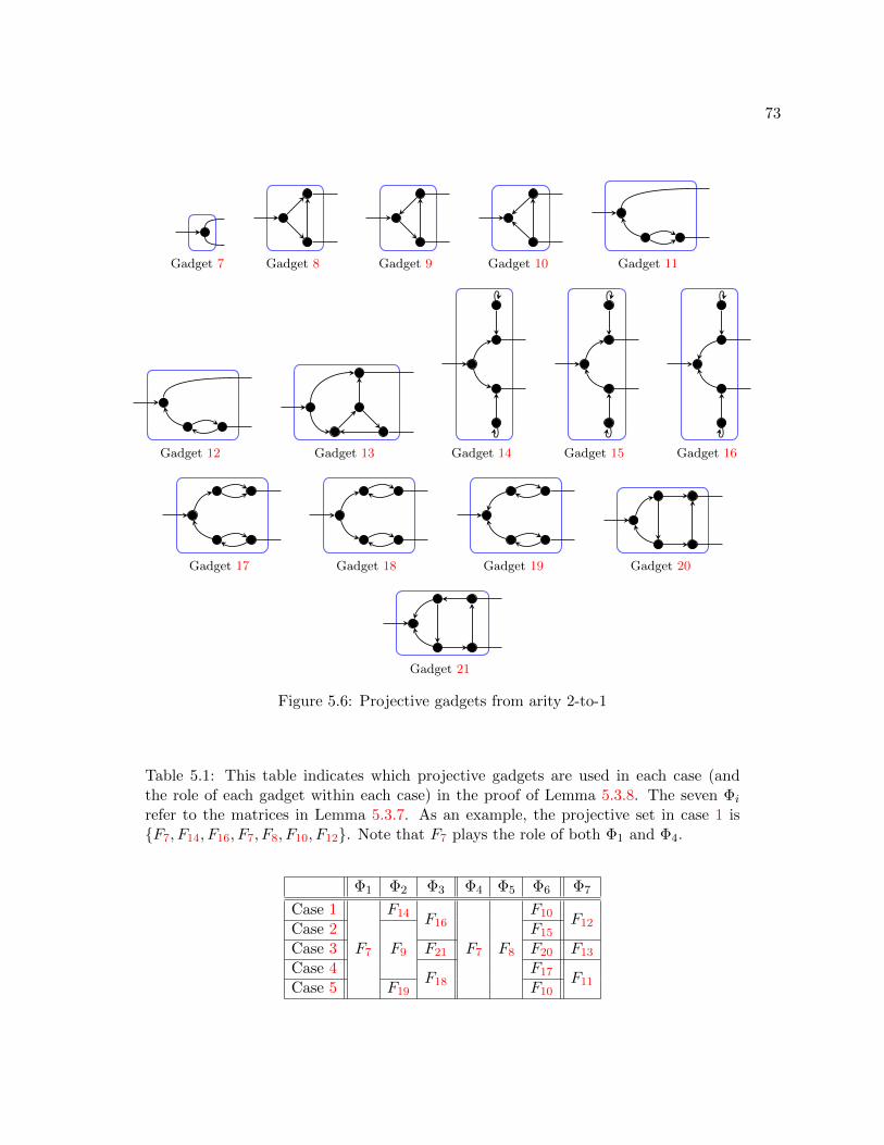
73

Gadget 7 Gadget 8 Gadget 9 Gadget 10 Gadget 11

Gadget 12 Gadget 13 Gadget 14 Gadget 15 Gadget 16

Gadget 17 Gadget 18 Gadget 19 Gadget 20

Gadget 21

Figure 5.6: Projective gadgets from arity 2-to-1

Table 5.1: This table indicates which projective gadgets are used in each case (andthe role of each gadget within each case) in the proof of Lemma 5.3.8. The seven Φi

refer to the matrices in Lemma 5.3.7. As an example, the projective set in case 1 isF7, F14, F16, F7, F8, F10, F12. Note that F7 plays the role of both Φ1 and Φ4.

Φ1 Φ2 Φ3 Φ4 Φ5 Φ6 Φ7

Case 1

F7

F14 F16

F7 F8

F10 F12Case 2F9

F15

Case 3 F21 F20 F13

Case 4F18

F17 F11Case 5 F19 F10

74

It suffices to exhibit projective gadget sets that satisfy the hypotheses of Lemma 5.3.7, which is

what we do.

Let Fi be the transition matrix of Gadget i for 7 ≤ i ≤ 21. There are five cases of projective

(f | =3)-gadget sets from arity 2-to-1. We omit the verification that each set of projective gadgets

forms a projective gadget set from arity 2-to-1 under its particular assumptions since this is a

straightforward linear algebra computation. The five cases are

1. wz 6= xy ∧ wxyz 6= 0 ∧ w3x+ wxyz + w2z2 + yz3 6= 0 ∧ x2 6= y2,

2. wz 6= xy ∧ wxyz 6= 0 ∧ w3x+ wxyz + w2z2 + yz3 6= 0 ∧ x = −y ∧ w3 6= −z3,

3. wz 6= xy ∧ wxyz 6= 0 ∧ w3x+ wxyz + w2z2 + yz3 = 0 ∧ x 6= y,

4. wz 6= xy ∧ w = 0 ∧ z 6= 0 ∧ x 6= y, and

5. wz 6= xy ∧ x = 0 ∧ y 6= 0.

Which projective gadgets are used in each case (and the role of each gadget within each case) can

be found in Table 5.1. In all five cases, the vector u in the kernels of Φ1, Φ2, and Φ3 is (0,−1, 1, 0)

and the vector v in the kernels of Φ4, Φ5, and Φ6 is (0,−x, y, 0).

All five cases utilize the assumption wz 6= xy, i.e., the edge signature is non-degenerate. Under

three additional disequality assumptions, the projective gadgets in row 1 of Table 5.1 have the

desired properties. The purpose of the remaining four cases is to handle the situation that these

three disequalities are not all true.

Case 2 retains two of the additional disequality assumptions but assumes that x2 = y2. Since

we are considering the asymmetric case, the only option is x = −y. By assumption, it is not the

case that x = −y∧w3 = −z3, so we have w3 6= −z3. Under these conditions, the projective gadgets

in row 2 of Table 5.1 have the desired properties.

Like cases 1 and 2, case 3 retains the assumption that no variable is zero but now considers

the case that the polynomial w3x+wxyz +w2z2 + yz3 is zero. Given that we are also considering

the asymmetric case (i.e. x 6= y), the projective gadgets in row 3 of Table 5.1 have the desired

properties.

Cases 4 and 5 handle the remaining case wz 6= xy ∧ wxyz = 0. The assumptions wz 6=

xy ∧ (w, z) 6= (0, 0)∧ (x, y) 6= (0, 0) imply that at most one of w, x, y, and z is 0. By switching the

75

θ

Gadget 22

ρ γ θ γ ρ

Gadget 23

Figure 5.7: Gadgets on the left used to simulate (0, 1, 1, 1).

role of 0 and 1 via the holographic transformation [ 0 11 0 ], the complexity of the case yz = 0 is the

same as the complexity of the case wx = 0. Therefore, we assume that yz 6= 0. Case 4 considers

w = 0, so z 6= 0 by assumption. Then still within the asymmetric case, the projective gadgets in

row 4 of Table 5.1 have the desired properties. Case 5 considers x = 0, so y 6= 0 by assumption

and the projective gadgets in row 5 of Table 5.1 have the desired properties.

These five cases cover all settings not excluded by the assumptions in the statement of the

lemma, so the proof is complete.

Once we have all unary signatures at our disposal, we can prove #P-hardness under most

settings. To do so, we make use of the following lemma.

Lemma 5.3.9 (Lemma 3.3 of [93]). Suppose that (a, b) ∈ C2 − (a, b) | ab = 1 − (0, 0) and let G

and R be finite signature sets where (a, 1, 1, b) ∈ G and =3∈ R. Further assume that Holant(G ∪

(Xi, Yi) | 0 ≤ i < m | R) ≤T Holant(G | R) for any Xi, Yi ∈ C and m ∈ Z+. Then Holant(G ∪

(0, 1, 1, 1) | R) ≤T Holant(G | R) and Holant(G | R) is #P-hard.

Lemma 5.3.10. Let w, x, y, z ∈ C, and let G and R be finite signature sets with (w, x, y, z) ∈ G

and =3∈ R. Suppose Holant(G ∪ (Xi, Yi) | 0 ≤ i < m | R) ≤T Holant(G | R) for any Xi, Yi ∈ C

and m ∈ Z+. Then Holant(G | R) is #P-hard unless wz = xy ∨ (w, z) = (0, 0) ∨ (x, y) = (0, 0).

Proof. Since Holant((0, 1, 1, 1) | =3), #VertexCover on 3-regular graphs, is #P-hard, we only

need to show how to simulate the signature (0, 1, 1, 1) on the left. The assumptions wz 6= xy ∧

(w, z) 6= (0, 0) ∧ (x, y) 6= (0, 0) imply that at most one of w, x, y, and z is 0. By switching the role

of 0 and 1 via the holographic transformation [ 0 11 0 ], the complexity of the case yz = 0 is the same

as the complexity of the case wx = 0. Therefore, we assume that yz 6= 0.

76

If w = 0, then Gadget 22 with θ = 1x( z

y2, 1z ) simulates (xz , 1, 1,

2zx ), which can in turn simulate

(0, 1, 1, 1) by Lemma 5.3.9. If x = 0, then Gadget 22 with θ = 1w ( 1

y ,yz2

) simulates (wy , 1, 1,2yw ),

which can in turn simulate (0, 1, 1, 1) by Lemma 5.3.9. If wx 6= 0∧wz = −xy, then Gadget 22 with

θ = 1xy (2x

w ,wx ) simulates (3w

y , 1, 1,3yw ), which can in turn simulate (0, 1, 1, 1) by Lemma 5.3.9. Finally

if wx 6= 0∧wz 6= xy ∧wz 6= −xy, then Gadget 23 with θ = wz+xywx(wz−xy)(−xw ,

wx ), γ = ( 1

wx ,−wx

yz(wz+xy)),

and ρ = 1wz−xy (xz,−wy) simulates (0, 1, 1, 1).

Remark. Let me explain how to pick θ, γ, and ρ in Gadget 23 given wx 6= 0∧wz 6= xy∧wz 6= −xy.

Initially, we set θ = (−xw ,wx ) so that the signature of Gadget 22 has 0 for its entry of Hamming

weight 0. Specifically, its signature matrix is (wz−xy)[

0 11 wz+xy

wx

]. This signature is also symmetric,

but its entries of Hamming weight 1 are different from its entry of Hamming weight 2. The purpose

of γ and ρ is to make these two entries equal. A factor of wz − xy has also appeared, so we cancel

it by setting θ = 1wz−xy (−xw ,

wx ).

Initially, we set ρ = (xz,−wy) so that, if we have ρ = θ in Gadget 22, then its signature matrix

is diagonal. Specifically, this matrix is (wz − xy)[wx 00 −yz

]. The contribution from γ in Gadget 23

will also be a diagonal matrix, so things are very easy to analyze now. Another factor of wz − xy

has appeared, so we cancel it by setting ρ = 1wz−xy (xz,−wy).

To simplify things further, we think of γ coming in two parts, γout and γin, such that γ =

γoutγin = γinγout. These are used to cancel terms on the “outside” (i.e. the ρ part) and the “inside”

(i.e. the θ part) respectively. By setting γout = ( 1wx ,

−1yz ), the signature matrix of the outside is I2.

Then we set γin = (1, wxwz+xy ) so that the signature matrix of the inside is wx

wz+xy [ 0 11 1 ]. To cancel

the remaining factor, we set θ = wz+xywx(wz−xy)(−xw ,

wx ).

By combining the Group Lemma (Lemma 5.3.6) with Lemma 5.3.8 and Lemma 5.3.10, we get

the following theorem.

Theorem 5.3.11. Let w, x, y, z ∈ C, and let G and R be finite signature sets where (w, x, y, z) ∈ G

and (=3) ∈ R. Suppose S is a finite set of recursive (G | R)-gates of arity d ≥ 1 with nonsingular

transition matrices. Let H be the group generated by the transition matrices of S, modulo scalar

matrices λI, for λ ∈ C − 0. If H has infinite order, then Holant(G | R) is #P-hard unless

77

x = y ∨ wz = xy ∨ (w, z) = (0, 0) ∨ (x, y) = (0, 0) ∨ (w3 = −z3 ∧ x = −y).

5.4 Statement of Main Result

Theorem 5.4.1. Let w, x, y, z ∈ C and f = (w, x, y, z). Then Holant(f | =3) is #P-hard unless

one of the following conditions holds, in which case, the problem is computable in polynomial time:

1. degenerate: wz = xy;

2. generalized disequality: w = z = 0;

3. generalized equality: x = y = 0;

4. holographic reduction to affine: wz = −xy ∧ w6 = εz6 ∧ x2 = εy2, where ε = ±1.

If the input is restricted to planar graphs, then another case becomes computable in polynomial time

but everything else remains #P-hard:

5. holographic reduction to matchgates: w3 = εz3 ∧ x = εy, where ε = ±1.

We prove the tractability part of Theorem 5.4.1 now.

Proof of tractability. In Case 1, case 2, and case 3, both signatures are of product type, so we are

done by Corollary 4.1.5.

For case 4, if w = z = 0, then this is already covered by case 2. Otherwise wz 6= 0 since

w6 = εz6, in which case we apply the holographic transformation[α 00 α2

]with α = εw2/z2, which

does not change the Holant value by Lemma 3.2.1. Note that α3 = εw6/z6 = 1. The edge signature

becomes (w, x, y, z)[α 00 α2

]⊗2= (α2w, x, y, αz), while =3 is unchanged since (

[α 00 α2

]−1)⊗3 = I8, the

8-by-8 identity matrix. This reduces to the case wz = −xy ∧ w2 = εz2 ∧ x2 = εy2. This edge

signature (as well as =3) is affine, so we are done by Theorem 4.2.6.

For case 5, if the input is restricted to planar graphs, apply the same holographic transformation

as in the previous case but with α = εz/w. Again, α3 = εz3/w3 = 1, so the edge signature becomes

(α2w, x, y, αz) and =3 is still unchanged. This reduces to the case w = εz ∧ x = εy. Then after a

further holographic transformation by the Hadamard matrix[

1 11 −1

], both signatures are matchgate

signatures, so we are done by Theorem 4.3.2.

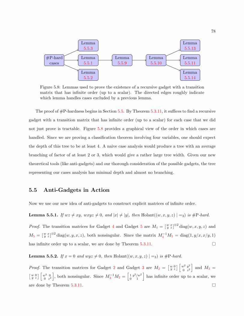
78

#P-hardcases

Lemma5.5.1

Lemma5.5.3

Lemma5.5.2

Lemma5.5.9

Lemma5.5.10

Lemma5.5.11

Lemma5.5.13

Lemma5.5.14

Figure 5.8: Lemmas used to prove the existence of a recursive gadget with a transitionmatrix that has infinite order (up to a scalar). The directed edges roughly indicatewhich lemma handles cases excluded by a previous lemma.

The proof of #P-hardness begins in Section 5.5. By Theorem 5.3.11, it suffices to find a recursive

gadget with a transition matrix that has infinite order (up to a scalar) for each case that we did

not just prove is tractable. Figure 5.8 provides a graphical view of the order in which cases are

handled. Since we are proving a classification theorem involving four variables, one should expect

the depth of this tree to be at least 4. A naive case analysis would produce a tree with an average

branching of factor of at least 2 or 3, which would give a rather large tree width. Given our new

theoretical tools (like anti-gadgets) and our thorough consideration of the possible gadgets, the tree

representing our cases analysis has minimal depth and almost no branching.

5.5 Anti-Gadgets in Action

Now we use our new idea of anti-gadgets to construct explicit matrices of infinite order.

Lemma 5.5.1. If wz 6= xy, wxyz 6= 0, and |x| 6= |y|, then Holant((w, x, y, z) | =3) is #P-hard.

Proof. The transition matrices for Gadget 4 and Gadget 5 are M4 = [w xy z ]⊗2 diag(w, x, y, z) and

M5 = [w xy z ]⊗2 diag(w, y, x, z), both nonsingular. Since the matrix M−1

4 M5 = diag(1, y/x, x/y, 1)

has infinite order up to a scalar, we are done by Theorem 5.3.11.

Lemma 5.5.2. If x = 0 and wyz 6= 0, then Holant((w, x, y, z) | =3) is #P-hard.

Proof. The transition matrices for Gadget 2 and Gadget 3 are M2 =[w 0y z

] [w2 y2

0 z2

]and M3 =[

w 0y z

] [w2 00 z2

], both nonsingular. Since M−1

3 M2 =[

1 y2/w2

0 1

]has infinite order up to a scalar, we

are done by Theorem 5.3.11.

79

Lemma 5.5.3. If w = 0 and xyz 6= 0, then Holant((w, x, y, z) | =3) is #P-hard.

Proof. The transition matrices for Gadget 3 and Gadget 6 are M3 =[

0 xy z

] [ 0 xyxy z2

]and M6 =

[0 xy z

][0 xyz3

xyz3 xy2z2+z5

], both nonsingular. Since M−1

3 M6 = z3[

1 y/z0 1

]has infinite order up to a scalar, we

are done by Theorem 5.3.11.

For the remainder of the proof of #P-hardness of Theorem 5.4.1, we use our anti-gadget tech-

nique in combination with Lemma 5.5.4, Lemma 5.5.5, and Lemma 5.5.6. In the contrapositive,

these lemmas provide sufficient conditions to conclude that a matrix has infinite order (up to a

scalar). Their proofs follow from a few observations, some of which are known as Vieta’s formulas.

For monic polynomials in C[X] of degree n with roots λi for 1 ≤ i ≤ n of the same nonnegative

norm r ∈ R, let ak ∈ C be the coefficient of Xk and σk the elementary symmetric polynomial of

degree k in λi/r for 1 ≤ i ≤ n, the norm one (scaled) roots.1 Thus ak = (−r)n−kσn−k. By having

norm one, σk = σn−kσn, ak = (−1)nrn−2kan−kσn, and |ak| = rn−2k|an−k|, for 0 ≤ k < n.

Lemma 5.5.4 (Lemma 4.4 in [93]). If both roots of X2 + a1X + a0 ∈ C[X] have the same norm,

then a1|a0| = a1a0. If further a0a1 6= 0, then Arg(a21) = Arg(a0) thus a2

1/a0 ∈ R+.

Lemma 5.5.5. If all roots of X4 + a3X3 + a2X

2 + a1X + a0 ∈ C[X] have the same norm, then

a2|a1|2 = |a3|2a2a0.

Lemma 5.5.6. If∑8

k=0 akXk ∈ C[X] is monic and all roots have the same norm, then a2

3|a1|2 =

|a7|2a52a2

0, a4|a2|2 = |a6|2a4a0, and |a3|2a2 = a6|a5|2a0.

Over 3-regular directed graphs, there are some symmetries under which the Holant is invariant.

The next lemma states these symmetries.

Lemma 5.5.7. Let G be a 3-regular directed graph. Then there exists a polynomial P with integer

coefficients in six variables, such that for any signature grid Ω having underlying graph G with

vertex signature =3 and edge signature (w, x, y, z),

Holant(Ω) = P (wz, xy, w3 + z3, x+ y, w3x+ yz3, w3y + xz3).

1This argument assumes r 6= 0. However, when r = 0, the conclusion still holds trivially.

80

Proof. Consider any 0, 1 vertex assignment σ with a nonzero valuation. If σ′ is the complement

assignment switching all 0’s and 1’s in σ, then for σ and σ′, we have the sum of valuations waxbyczd+

wdxcybza for some a, b, c, d. Here a (resp. d) is the number of edges connecting two degree 3 vertices

both assigned 0 (resp. 1) by σ. Similarly, b (resp. c) is the number of edges from one degree 3 vertex

to another that are assigned 0 and 1 (resp. 1 and 0), in that order, by σ. We note that

waxbyczd + wdxcybza =

(wz)min(a,d)(xy)min(b,c)(w|a−d|y|b−c| + x|b−c|z|a−d|

)a > d XOR b > c

(wz)min(a,d)(xy)min(b,c)(w|a−d|x|b−c| + y|b−c|z|a−d|

)otherwise.

We prove a ≡ d (mod 3) inductively. For the all-0 assignment, this is clear since every edge

contributes a factor w and the number of edges is divisible by 3 for a 3-regular graph. Now starting

from any assignment, if we switch the assignment on one vertex from 0 to 1, it is easy to verify

that it changes the valuation from waxbyczd to wa′xb′yc′zd′, where a − d = a′ − d′ + 3. As every

0, 1 assignment is obtainable from the all-0 assignment by a sequence of switches, the conclusion

a ≡ d (mod 3) follows.

Now

waxbyczd + wdxcybza =

(wz)min(a,d)(xy)min(b,c)(w3ky` + x`z3k

)a > d XOR b > c

(wz)min(a,d)(xy)min(b,c)(w3kx` + y`z3k

)otherwise

for some k, ` ≥ 0. Consider w3ky` + x`z3k (the other case is similar). Two simple inductive steps

w3ky`+1 + x`+1z3k =(w3ky` + x`z3k

)(x+ y)− xy

(w3ky`−1 + x`−1z3k

)w3(k+1)y` + x`z3(k+1) =

(w3ky` + x`z3k

) (w3 + z3

)− (wz)3

(w3(k−1)y` + x`z3(k−1)

)

(when combined with the other case) show that the Holant is a polynomial P (wz, xy, w3 + z3, x+

y, w3x+ yz3, w3y + xz3) with integer coefficients.

Assuming non-degeneracy of (w, x, y, z), Lemma 5.5.1, Lemma 5.5.2, and Lemma 5.5.3 give

#P-hardness unless two (or more) of w, x, y, and z are 0 or none are 0 and |x| = |y|. If any

81

two (or more) of variables are 0, then the problem is tractable, as proved after Theorem 5.4.1.

Therefore, the dichotomy in Theorem 5.4.1 holds unless wxyz 6= 0 and |x| = |y|. In accordance

with Lemma 5.5.7, we make a change of variables to A = wz, B = xy, C = w3 + z3, D = x + y,

E = w3x + yz3, and F = w3y + xz3. Since the complexity of a Holant remains the same under

multiplication by a nonzero constant to any signature, we normalize so that |x| = 1 and x = y

without repeatedly stating this as an assumption. Thus B = 1 and D = x + y ∈ [−2, 2] with

D2 = 4 corresponding to the symmetric case: x = y. A degenerate edge signature now means

A = 1. Additionally, notice that E + F = CD and EF = −4A3B + BC2 + A3D2. Theorem 5.4.1

can also be stated in these symmetrized variables.

Theorem 5.5.8. Suppose w, x, y, z ∈ C. Then Holant((w, x, y, z) | =3) is #P-hard except in the

following cases, for which the problem is computable in polynomial time:

1. wz = xy ⇐⇒ A = B;

2. w = z = 0 ⇐⇒ A = C = 0;

3. x = y = 0 ⇐⇒ B = D = 0;

4. wz = −xy ∧ w6 = z6 ∧ x2 = y2 ⇐⇒ A = −B ∧ 4A3C = C3 ∧ 4BD = D3;

5. wz = −xy ∧ w6 = −z6 ∧ x2 = −y2 ⇐⇒ A = −B ∧ 2A3 = C2 ∧ 2B = D2.

If the input is restricted to planar graphs, then two more cases become tractable but all other cases

remain #P-hard:

6. w3 = z3 ∧ x = y ⇐⇒ 4A3 = C2 ∧ 4B = D2;

7. w3 = −z3 ∧ x = −y ⇐⇒ C = D = 0.

Remark. One way to convert a polynomial in w, x, y, z to a polynomial in A,B,C,D,E, F is to

use a Grobner basis. We tried that here, but it did not give us the kinds of polynomials that we

wanted. Intuitively, we want polynomials that look as though they were obtained by applying the

proof of Lemma 5.5.7. Not only does the result of the Grobner basis algorithm depend on the

order in which the variables are considered, but we have an underdetermined system because we

are converting from only four variables to six. In the end, I wrote my own program to do the

conversion, which tried to minimize the occurrences of E and F as much as possible.

Now we continue with the proof of #P-hardness.

82

Gadget 24

Figure 5.9: Another unary recursive gadget

Lemma 5.5.9. If D2 6= 4, and A 6∈ R, then Holant((w, x, y, z) | =3) is #P-hard.

Proof. The transition matrices for Gadget 24 and Gadget 3 are M24 = [w yx z ]

[w2 xyxy z2

]and M3 =

[w xy z ]

[w2 xyxy z2

]. Both matrices have determinant (A − 1)2(A + 1), which is nonzero since A is not

real. Then N = M24M−13 has determinant 1 and trace

tr

w y

x z

w x

y z

−1 =

2wz − x2 − y2

wz − xy=

2A−D2 + 2

A− 1,

which is nonzero since A is not real. If the eigenvalues of N have distinct norms, then it has infinite

order up to a scalar and we are done by Theorem 5.3.11, so assume that its eigenvalues are of

equal norm. Then Lemma 5.5.4 says that tr(N)2

detN = (2A−D2+2)2

(A−1)2∈ R+. Taking square roots, we have

2A−D2+2A−1 ∈ R, which implies that −D

2+4A−1 ∈ R. Since D2 6= 4, this gives A ∈ R, a contradiction.

Unary recursive gadgets, such as the ones used in the proof of Lemma 5.5.9, are quite useful

for proving #P-hardness when variables like A = wz are complex. When all variables are real, the

conclusion of Lemma 5.5.4 is weak (though one can still prove #P-hardness using a related lemma

with significant effort in the symmetric case [48]). For complex variables in the symmetric case, [93]

showed that using higher arity (namely binary) recursive gadgets can give a much simpler proof of

#P-hardness. The next lemma continues this pattern with the first ever use of ternary recursive

gadgets.

Gadget 25 Gadget 26

Figure 5.10: Ternary recursive gadgets

83

Lemma 5.5.10. If A2 6= 1, AD 6= 0, and D2 6= 4, then Holant((w, x, y, z) | =3) is #P-hard.

Proof. The determinants of the 8-by-8 transition matrices of Gadget 25 and Gadget 26 are both

A2(A− 1)4 6= 0. If N = M−125 M26 has any two eigenvalues with distinct norms, then it has infinite

order up to a scalar and we are done by Theorem 5.3.11. Thus assume that all eight eigenvalues

of N have the same norm. Then by Lemma 5.5.6, we know that several equations hold among the

coefficients of its characteristic polynomial. After scaling by the nonzero factor A(A − 1), these

coefficients for A(A− 1)N are

a7 = (A− 1)(AD2 + 2A+ 2)

a6 = (A− 1)2(5A2D2 − 3A2 + 2AD2 + 2A+ 1)

a5 = A(A− 1)3(A2D4 + 5A2D2 − 6A2 + 7AD2 − 6A+D2)

a4 = A2(A− 1)4(3A2D4 − 4A2D2 + 4A2 +AD4 + 4AD2 − 4A+ 2D2 − 2)

a3 = A3(A− 1)5(2AD4 + 3A2D4 − 6A2D2 + 6A2 − 4AD2 + 6A+D2)

a2 = A4(A− 1)6(A2D4 +A2D2 − 3A2 +AD4 − 2AD2 + 2A+ 1)

a1 = A6(A− 1)7(2AD2 − 2A+D2 − 2)

a0 = A8(A− 1)8.

Amazingly, C, E, and F do not appear.2 Lemma 5.5.9 shows #P-hardness unless A ∈ R, so assume

that A ∈ R. Because A,D ∈ R, the equations in Lemma 5.5.6 are simplified by the disappearance

of norms and conjugates. Using CylindricalDecomposition in Mathematica, we conclude that

there are no solutions under our assumptions, which is a contradiction.

Remark. Lemma 5.5.6 gives three equations that follow from the roots all having the same norm.

We had found five equations, but these three were sufficient to prove Lemma 5.5.10. Even with the

two additional equations, we did not see a way to prove the lemma without using Mathematica.

We explain the meaning of the assumptions in Lemma 5.5.10 after the next lemma, which

considers the same assumptions except that D = 0 and C 6= 0.

2The runtime of CylindricalDecomposition is a double exponential in the number of variables, so it is crucialthat our query include as few variables as possible.

84

Gadget 27 Gadget 28

Gadget 29 Gadget 30 Gadget 31 Gadget 32

Figure 5.11: Binary recursive gadgets

Lemma 5.5.11. If A2 6= 1, AC 6= 0, and D = 0, then Holant((w, x, y, z) | =3) is #P-hard.

Proof. Lemma 5.5.9 shows #P-hardness unless A ∈ R, so assume that A ∈ R. The transition

matrix for Gadget 27 is M27 = [w xy z ]⊗2 diag(w, x, y, z) and has determinant A(A − 1)2 6= 0. If

M27 has any two eigenvalues with distinct norms, then it has infinite order up to a scalar and we

are done by Theorem 5.3.11, so assume that all eigenvalues have the same norm. However, the

coefficients of the characteristic polynomial of M27, which are

(a3, a2, a1, a0) =(−C, (A+ 1)2(A− 1),−(A− 1)2C,A(A− 1)4

),

do not satisfy the conclusion of Lemma 5.5.5 under the assumptions, a contradiction.

The case A = 1 is degenerate (thus tractable), the case A = 0 is covered in Lemma 5.5.3, and

recall that D2 = 4 corresponds to the symmetric case [93], so now we assume A /∈ 0, 1 ∧D2 6= 4.

Lemma 5.5.10 handled A 6= −1 and D 6= 0 while Lemma 5.5.11 handled A 6= −1 ∧D = 0 ∧ C 6= 0.

We note that C = D = 0 is tractable over planar graphs. Now we focus on the case A = −1.

The next two proofs of #P-hardness (the proofs of Lemma 5.5.13 and Lemma 5.5.14) make use

of the following technical lemma.

Lemma 5.5.12. Let c ∈ C and ε = ±1. Then the only solutions to the equation (c+ 2ε)c = ε(c+2ε)

are the trivial solutions c ∈ −2ε, ε.

85

Proof. Assume that c 6= −2ε. Now we show that c = ε. Taking norms, we see that |c| = 1. Then

simplifying (c+ 2ε)c = ε(c+ 2ε) using cc = |c|2 = 1 yields c = ε as claimed.

Lemma 5.5.13. If A = −1 and E 6∈ 0,±2i, then Holant((w, x, y, z) | =3) is #P-hard.

Proof. The transition matrices of Gadget 28, Gadget 29, and Gadget 31 are

M28 =

w x

y z

⊗2

diag(w, y, x, z)

w y

x z

⊗2

diag(w, x, y, z)

M29 =

w x

y z

⊗2

w4 + wxy2 w2xy + xy2z 0 0

w2xy + xy2z wxyz + yz3 0 0

0 0 w3x+ wxyz wx2y + xyz2

0 0 wx2y + xyz2 x2yz + z4

M31 =

w x

y z

⊗2

diag(w, y, x, z)

I2 ⊗

w x

y z

w2 + yz 0

0 wx+ z2

with detM28 = 28, detM31 = −26E2, and detM29 = 26(E2 + 4), so all are nonsingular. Let

N1 = M−128 M31 and N2 = M−1

28 M29. The coefficients of the characteristic polynomials of −24N1

and 24N2 are respectively

(a3, a2, a1, a0) =(−4, E2 + 12,−4(E2 + 4), 4(E2 + 4)

)(a3, a2, a1, a0) =

(4,−E2 + 8,−4E2,−4E2

).

If N1 (resp. N2) has any two eigenvalues with distinct norms, then N1 (resp. N2) has infinite order

up to a scalar and we are done by Theorem 5.3.11, so assume that all eigenvalues of N1 (resp. N2)

have the same norm. Then by Lemma 5.5.5, we have two equations relating these coefficients.

However, after a change of variables by c = (E2 + 4)/4 (for the coefficients of N1) and c = E2/4

(for the coefficients of N2), Lemma 5.5.12 says that the only solutions to both equations require

E ∈ 0,±2i, a contradiction.

The next lemma is similar to Lemma 5.5.13 with E in place of F .

86

Lemma 5.5.14. If A = −1 and F 6∈ 0,±2i, then Holant((w, x, y, z) | =3) is #P-hard.

Proof. The transition matrices of Gadget 28, Gadget 30, and Gadget 32 are

M28 =

w x

y z

⊗2

diag(w, y, x, z)

w x

y z

⊗2

diag(w, x, y, z)

M30 =

w x

y z

⊗2

w4 + wx2y w2xy + x2yz 0 0

w2xy + x2yz wxyz + xz3 0 0

0 0 w3y + wxyz wxy2 + xyz2

0 0 wxy2 + xyz2 xy2z + z4

M32 =

w x

y z

⊗2

diag(w, x, y, z)

I2 ⊗

w x

y z

w2 + xz 0

0 wy + z2

.

The rest of the proof uses the same reasoning as the proof of Lemma 5.5.13 with Gadget 29 and

Gadget 31 replaced by Gadget 30 and Gadget 32 respectively.

All remaining cases, those for which A = −1 and E,F ∈ 0,±2i, imply tractability. Since this

is not immediately obvious, we prove this next. As pointed out after Lemma 5.5.7, the following

equations hold and are used frequently below. They simplify to

E + F = CD (5.5.1)

EF = −4A3B +BC2 +A3D2 = 4 + C2 −D2 (5.5.2)

when A = −1 and B = 1. These next four lemmas cover all possibilities of E,F ∈ 0,±2i as

follows:

Lemma 5.5.15: Both zero;

Lemma 5.5.16: Both nonzero and equal;

Lemma 5.5.17: Both nonzero and not equal;

Lemma 5.5.18: Exactly one zero.

87

Lemma 5.5.15. If A = −1∧E = F = 0, then (D = 0∧C2 = −4) or (D2 = 4∧C = 0), which are

both tractable.

Proof. Since 0 = E + F = CD, either C or D is zero. In either case, simplifying (5.5.2) gives the

desired result and is covered by tractable case 4 in Theorem 5.5.8.

Lemma 5.5.16. If A = −1 ∧ E = F = ±2i, then C2 = −4 ∧D2 = 4, which is tractable.

Proof. Using wz = A = −1 and xy = B = 1, we multiply ±2i = E = w3x + yz3 by w3y to get

y2±2iw3y−w6 = 0. Similarly, multiplying ±2i = F = w3y+xz3 by w3x gives x2±2iw3x−w6 = 0.

This is the same quadratic polynomial with x and y as indeterminates. Its discriminant is zero, so

x = y which means that D2 = 4. Simplifying (5.5.2) yields C2 = −4 as required. This is covered

by tractable case 4 in Theorem 5.5.8.

Lemma 5.5.17. If A = −1 ∧ E = −F = ±2i, then C = D = 0, which is tractable.

Proof. Since 0 = E + F = CD, either C or D is zero. Simplifying (5.5.2) gives C2 = D2, so both

C and D are zero. This is covered by tractable case 4 in Theorem 5.5.8.

Lemma 5.5.18. If A = −1 ∧ ((E = ±2i ∧ F = 0) ∨ (E = 0 ∧ F = ±2i)), then D2 = 2 ∧ C2 = −2,

which is tractable.

Proof. Since ±2i = E + F = CD, neither C or D is zero. Squaring this equation and solving for

C2 gives C2 = −4/D2. In (5.5.2), first we substitute for C2 to conclude that D2 = 2 and then

substitute for D2 to conclude that C2 = −2. This is tractable case 5 in Theorem 5.5.8.

At this point, every setting of the variables has either been proven tractable over planar graphs

or #P-hard. So far, all our hardness proofs originate from #VertexCover over 3-regular graphs,

which is Holant((0, 1, 1, 1) | =3). Recall that #VertexCover is #P-hard even for 3-regular planar

graphs [144] and notice that all of our gadget constructions are planar, including our interpolation

construction in the Group Lemma (see Figure 5.2c). Therefore, all of the #P-hardness results

proved so far still apply when the input is restricted to planar graphs. There are, however, some

cases where the problem is #P-hard in general, yet is polynomial time computable when restricted

to planar graphs. We analyze this case next using a lemma from [93] that can also be found in [92].

88

Gadget 33 Gadget 34

Figure 5.12: Gadgets on the left with a symmetric signature.

Lemma 5.5.19 (Lemma 33 of [92]). If w /∈ 0,±1,±i, then Holant((w, 1, 1, w) | =3) is #P-hard.

Lemma 5.5.20. If w /∈ 0,±1,±i, then Holant((w, 1,−1,−w) | =3) is #P-hard.

Proof. Gadget 33 and Gadget 34 simulate two symmetric signatures on the left. Using Reduce in

Mathematica, we conclude that at least one of the gadgets satisfies the hypothesis for #P-hardness

from Lemma 5.5.19.

Lemma 5.5.21. Suppose w3 = εz3 ∧ x = εy where ε = ±1. If x 6= 0 ∧ w/x /∈ 0,±1,±i, then

Holant((w, x, y, z) | =3) is #P-hard.

Proof. If wz 6= 0, then we apply the holographic transformation[α 00 α2

]with α = εz/w, which does

not change the Holant value by Lemma 3.2.1. As in the proof of tractability, this reduces to the

case w = εz ∧ x = εy. This equivalence still holds if wz = 0. We then normalize x = 1 (since it

is nonzero) and replace z with εw to obtain the edge signature (w/x, 1, ε, εw/x). Depending on ε,

this case is either covered in Lemma 5.5.19 (when ε = 1) or in Lemma 5.5.20 (when ε = −1), so

we are done.

5.6 Anti-Gadgets and Previous Work

To further appreciate the usefulness of anti-gadgets, we show how this technique sheds new light

on previous results.

One can find failure conditions for a binary recursive gadget using the following lemma.

Lemma 5.6.1. Let G be a binary recursive gadget having nonsingular transition matrix M . Then

M ii≥0 is a sequence of pairwise linearly independent signatures unless a2|a1|2 − |a3|2a2a0 = 0,

where x4 + a3x3 + a2x

2 + a1x+ a0 is the characteristic polynomial of M .

89

Gadget 35 Gadget 36

Figure 5.13: Recursive gadgets from [37] on k-regular graphs. Bold edges representparallel edges. In Gadget 35 (resp. Gadget 36), the multiplicity is k − 2 (resp. k − 4)so that the vertices have degree k.

Analyzing a failure condition such as a2|a1|2 − |a3|2a2a0 = 0 simultaneously for several gadgets

is quite difficult, even with the aid of symbolic computation. Previous work [37, 36] relied heavily

on miraculous cancellations in the failure conditions to contend with this. For example, consider the

two gadgets in Figure 5.13. They are from [37], where symmetric (i.e. x = y) signatures (w, x, y, z)

were considered on k-regular graphs.

After a change of variables X = wzx−2 and Y = (w/x)3 +(z/x)3 and making a few assumptions

to guarantee that M35 and M36 are nonsingular (which we omit in this discussion), the failure

conditions of Gadget 35 and Gadget 36 (when restricted to the real numbers) simplify to

(X − 1)3(Xk−2 − 1)(Xk−2(X + 1)2(Xk−1 +Xk−2 +X + 3Y + 1)− Y 3) = 0,

X3(X − 1)3(Xk−4 − 1)(Xk−2(X + 1)2(X2 +Xk−2 +X + 3Y +Xk−3)− Y 3) = 0.

Assuming that both gadgets fail and X /∈ 0,±1, this gives two polynomial expressions for Y 3.

Setting these equal to each other and refactoring results in the contradiction Xk−2(X + 1)3(X −

1)(Xk−3−1) = 0, implying that either one or the other gadget works. At the time of this discovery,

it was a mystery whether there was any underlying explanation for such miraculous cancellations.

Now we see how anti-gadgets reveal a better understanding of this same gadget pair.

By assuming that M35 fails to produce an infinite set of pairwise linearly independent signatures,

we have an explicit recursive gadget for M−135 . Then M−1

35 M36 = diag(1, X,X, 1) clearly produces an

infinite set of pairwise linearly independent signatures unless X is zero or a root of unity. Note that

in the “gadget language” of M−135 M36, the two leading directed edges of Gadget 35 and Gadget 36

simply annihilate each other, as do k − 4 copies of the vertical edge. The signatures =3 at the

90

Gadget 37 Gadget 38

Figure 5.14: Recursive gadgets from [36] on k-regular graphs for k even. The gadgetsare pictured for k = 4 but generalize to all even k ≥ 4 by adding self loops to thevertices.

degree 3 vertices force the matrix M−135 M36 to be diagonal. Thus, with almost no effort we have

a strictly stronger result (i.e. over the complex numbers) through the use of an anti-gadget. This

also shows that the anti-gadget concept is useful in the symmetric setting as well as the asymmetric

setting.

In [36], a similarly fantastic cancellation occurred involving Gadget 37 and Gadget 38 (see

Figure 5.14). They form a suitable gadget and anti-gadget pair, as M−137 M38 is a diagonal matrix.

While this diagonal matrix is not as easy to analyze as the previous example, anti-gadgets would

inform the search for such useful gadgets, even if the analysis is carried out with different techniques.

5.7 Closing Thoughts

General purpose binary starter gadgets In Section 5.3, we said

[projective gadget sets permit] much more freedom in gadget constructions, and this

power is used crucially in the proof of our dichotomy theorem.

We definitely believed this at the time, but now I think there is a sense in which this is a bit over

stated. Let me explain.

When I begin this work of generalizing [94, 93], I decided not to use the linear interpolation

that they used. They were unable to find general purpose binary starter gadgets, which made their

proof more difficult. In his thesis [92, p. 69], Michael Kowalczyk suggested this difficulty could be

avoided by using the circular interpolation construction from their later work [37, 36]. They had

used it to overcome a parity restriction when the arity of Equality signature is even (in which

case, one can only construct ((w, x, y, z) | =k)-gates with an even number of dangling edges). I

91

took this suggestion.

Using the circular construction when doing k-dimensional interpolation brings its own challenge.

Namely, how to construct projective gadgets from arity k-to-1? We decisively solved this problem

by Lemma 5.3.3, which says that it suffices to find projective gadgets from arity 2-to-1. This is what

the previous [94, 93] work had called finisher gadgets, so given this lemma, we now had strictly

fewer conditions to satisfy to prove our dichotomy than [94, 93]. However, it is better than this.

After publishing [39], we realized that we could have simplified our proof. Lemma 5.3.3 can be

strengthened to say that it suffices to find projective gadgets from arity 1-to-0. (These projective

gadgets only have one dangling edge, so this is only possible when the arity of the Equality

signature is odd.) Then we can get drastically simpler versions of Lemma 5.3.7 and Lemma 5.3.8.

Instead of needing all the projective gadgets from arity 2-to-1 in Figure 5.6 and the projective

gadget sets they form in Table 5.1, we should be able to find projective gadget set from arity

1-to-0.

Projective gadgets from arity 1-to-0 are the same as unary starter gadgets in [94, 93], and

they had no problem finding general purpose unary starter gadgets, so I expect that we could also

find general purpose unary starter gadgets in our setting. Now look more closely at the proof of

Lemma 5.3.3. The projective gadget F from arity 2-to-1 was used to create the projective gadget

F ′ = I2k−2 ⊗ F from arity k-to-1. This was of creating F ′ makes it easy to reason about, but

any way of tensoring F and identity matrices (and ending up with a 2k−1-by-2k) should work. In

particular, we could use F ′ = F ⊗I2k−1 in the strengthening of Lemma 5.3.3 when F is a projective

gadget from arity 1-to-0.

This construction actually yields general purpose binary starter gadgets from general purpose

unary starter gadgets, which solve the open question Kowalczyk has posed in his thesis. The

final construction is not really the circular interpolation construction nor is it really the linear

interpolation construction. Instead, it is some hybrid of the two and superior to both.

Conjecture for generalization Based on the result in this chapter and the results in [37, 36],

I make the following conjecture.

92

Conjecture 5.7.1. Let w, x, y, z ∈ C and f = (w, x, y, z). Suppose k ≥ 1 is an integer. Then

Holant(f | =k) is #P-hard unless one of the following conditions holds, in which case, the problem

is computable in polynomial time:

1. k ≤ 2;

2. degenerate: wz = xy;

3. generalized disequality: w = z = 0;

4. generalized equality: x = y = 0;

5. holographic reduction to affine: wz = −xy ∧ w2k = εkz2k ∧ x2 = εy2, where ε = ±1.

If the input is restricted to planar graphs, then another case becomes computable in polynomial time

but everything else remains #P-hard:

6. holographic reduction to matchgates: wk = εkzk ∧ x = εy, where ε = ±1.

I can show that the conjectured tractable cases are indeed so.

Proof of tractability. For case 1, the Holant is a product over disconnected components, and on

each connected component, the Holant can be computed with matrix product and trace. In Case 1,

case 2, and case 3, both signatures are of product type, so we are done by Corollary 4.1.5.

For case 5, we do a holographic transformation by [ 1 00 α ] with α = (εkw2/z2)1/4. Reusing variable

names, the transformed edge signature f = (w, x, y, z) satisfies wz = −xy ∧w2 = εkz2 ∧ x2 = εky2,

which is affine. The Equality signature =k is transformed to [1, 0, . . . , 0, αk], which is affine since

α4k = 1. Thus we are done by Theorem 4.2.6.

For case 6, we do a holographic transformation by [ 1 00 α ] with α = (εkw/z)1/2. Reusing variable

names, the transformed edge signature f = (w, x, y, z) satisfies w = εkz ∧ x = εky. The Equality

signature =k is transformed to [1, 0, . . . , 0, αk]. Since α2k = 1, both of these signatures become

matchgate signatures after a further holographic transformation by the Hadamard matrix[

1 11 −1

],

so we are done by Theorem 4.3.2.

A proof of hardness for the remaining cases should follow without too much difficulty by using

the Pl-#CSP2(F) dichotomy recently proved in [27].

93

Chapter 6

Dichotomy for Holant Problems over

Planar 4-Regular Graphs

For Holant problems, it is important to understand the complexity of the small arity cases first.

In this chapter, we prove a dichotomy theorem for a symmetric signature of arity 4 with complex

weights in the planar Holant framework. This result is used to obtain both the Holant dichotomy

in Chapter 7 and the planar #CSP dichotomy in Chapter 8. To prove this result, we improve

known interpolation techniques in both the one- and two-dimensional settings. In one dimension,

we provide a tight characterization of when it succeeds. We apply this result alongside the anti-

gadget technique from Chapter 5 and a new technique called planar pairing. The case for two

dimensions involves a demanding interpolation step using asymmetric signatures. We found that

in order to prove a dichotomy for a symmetric signature, we must consider asymmetric ones. In

particular, we prove that counting Eulerian orientations over planar 4-regular graphs is #P-hard.

The reduction is from the problem of evaluating the Tutte polynomial of a planar graph at the

point (3, 3). Part of this work was published in [29, 30] and part of it was published in [73, 74].

94

6.1 Background

For Holant problems, it is important to understand the complexity of the small arity cases first. We

use the following theorem about edge-weighted signatures on degree prescribed graphs. Specifically,

we apply it with G = =4. See also Theorem 22 in [92], which contains a proof.

Theorem 6.1.1 (Theorem 3 in [36]). Let S ⊆ Z+ contain k ≥ 3, let G = =k| k ∈ S, and let

d = gcd(S). Suppose f0, f1, f2 ∈ C. Then Holant([f0, f1, f2] | G) is #P-hard unless one of the

following conditions hold, in which case the problem is computable in polynomial time:

1. f0f2 = f21 ;

2. f0 = f2 = 0;

3. f1 = 0;

4. f0f2 = −f21 ∧ f2d

0 = f2d2 .

If the input is restricted to planar graphs, then the problem remains #P-hard unless

5. fd0 = fd2 ,

in which case the problem is computable in polynomial time.

Theorem 6.1.1 is very explicit, but its restatement as Theorem 6.1.2 is more conceptual. Let

Tk =

[ 1 00 ω ] ∈ C2×2 | ωk = 1

.

Theorem 6.1.2 (Theorem 3 in [36]). Let S ⊆ Z+ contain k ≥ 3, let G = =k| k ∈ S, and let

d = gcd(S). Suppose f is a non-degenerate, symmetric, complex-valued binary signature in Boolean

variables. Then Holant(f | G) is #P-hard unless one of the following conditions hold, in which case

the problem is computable in polynomial time:

1. f ∈P;

2. there exists T ∈ T4d such that T⊗2f ∈ A ;

If the input is restricted to planar graphs, then the problem remains #P-hard unless

3. there exists T ∈ T2d such that T⊗2f ∈[

1 11 −1

]M ,

in which case the problem is computable in polynomial time.

When f is a symmetric signature of arity 3 with complex weights, Cai, Huang, and Lu [35,

Theorem 3] gave a dichotomy for Holant(f) while Cai, Lu, and Xia [46, special case of Theorem V.1]

95

gave a dichotomy for Pl-Holant(f). We state their dichotomies as a single result.

Theorem 6.1.3. If f is a non-degenerate, symmetric, complex-valued signature of arity 3 in

Boolean variables, then Holant(f) is #P-hard unless f is A -transformable or P-transformable

or vanishing, in which case, the problem is computable in polynomial time. If the input is restricted

to planar graphs, then the problem remains #P-hard unless M -transformable, in which case, the

problem is computable in polynomial time.

In this chapter, we use the dichotomy for Pl-Holant(f) prove the planar dichotomy for any

signature of arity 4 with complex weights. This result is used to obtain both the Holant dichotomy

in Chapter 7 and the planar #CSP dichotomy in Chapter 8. To prove this result, we improve known

interpolation techniques in both the one- and two-dimensional settings. Some previous dichotomy

theorems were for Holant problems with real weights [48, 37, 46, 80]. A dichotomy for complex

weights is more technically challenging. The proof technique of polynomial interpolation often has

infinitely many failure cases in C corresponding to the infinitely many roots of unity, which prevents

a brute force analysis of failure cases. This increased difficulty requires us to develop new ideas to

bypass previous interpolation proofs.

For interpolation in one dimension, we provide a tight characterization of when it succeeds.

When it fails is the perfect time to use the anti-gadget technique from Chapter 5. We also introduce

the notion of planar pairings to build reductions. We show that every planar 3-regular graph has

a planar pairing and that one can be efficiently computed. By combining these three techniques,

we show that counting complex-weighted matchings over planar 4-regular graphs is #P-hard.

Our interpolation result in two dimensions involves a demanding interpolation step using asym-

metric signatures. We found that in order to prove a dichotomy for a symmetric signature, we must

consider asymmetric ones. Huang and Lu [80] proved that counting Eulerian orientations is #P-

hard over 4-regular graphs but left open its complexity when the input is also planar. We perform

a planar interpolation with a rotationally invariant signature to show that this problems remains

#P-hard when further restricted to planar graphs. The reduction is from the problem of evaluating

the Tutte polynomial of a planar graph at the point (3, 3), which has a natural expression in the

Holant framework.

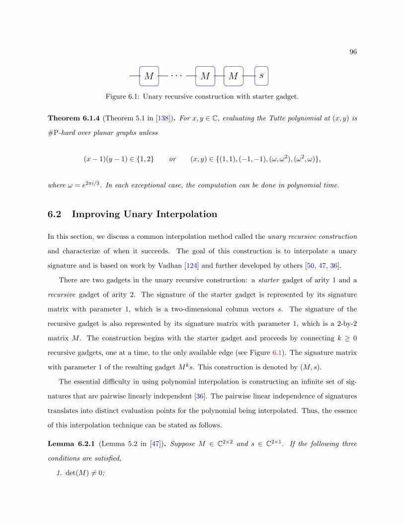
96

M M · · · M M s

Figure 6.1: Unary recursive construction with starter gadget.

Theorem 6.1.4 (Theorem 5.1 in [138]). For x, y ∈ C, evaluating the Tutte polynomial at (x, y) is

#P-hard over planar graphs unless

(x− 1)(y − 1) ∈ 1, 2 or (x, y) ∈ (1, 1), (−1,−1), (ω, ω2), (ω2, ω),

where ω = e2πi/3. In each exceptional case, the computation can be done in polynomial time.

6.2 Improving Unary Interpolation

In this section, we discuss a common interpolation method called the unary recursive construction

and characterize of when it succeeds. The goal of this construction is to interpolate a unary

signature and is based on work by Vadhan [124] and further developed by others [50, 47, 36].

There are two gadgets in the unary recursive construction: a starter gadget of arity 1 and a

recursive gadget of arity 2. The signature of the starter gadget is represented by its signature

matrix with parameter 1, which is a two-dimensional column vectors s. The signature of the

recursive gadget is also represented by its signature matrix with parameter 1, which is a 2-by-2

matrix M . The construction begins with the starter gadget and proceeds by connecting k ≥ 0

recursive gadgets, one at a time, to the only available edge (see Figure 6.1). The signature matrix

with parameter 1 of the resulting gadget Mks. This construction is denoted by (M, s).

The essential difficulty in using polynomial interpolation is constructing an infinite set of sig-

natures that are pairwise linearly independent [36]. The pairwise linear independence of signatures

translates into distinct evaluation points for the polynomial being interpolated. Thus, the essence

of this interpolation technique can be stated as follows.

Lemma 6.2.1 (Lemma 5.2 in [47]). Suppose M ∈ C2×2 and s ∈ C2×1. If the following three

conditions are satisfied,

1. det(M) 6= 0;

97

2. s is not a column eigenvector of M (nor the zero vector);

3. the ratio of the eigenvalues of M is not a root of unity;

then the vectors in the set V = Mksk≥0 are pairwise linearly independent.

Clearly the first condition is necessary. The second condition is equivalent to det([s Ms]) 6= 0,

which is necessary since it checks the linear dependence of the first two vectors in V .

The unary recursive construction can be generalized to larger dimensions, where the starter

gadget has arity d and the recursive gadget has arity 2d [93]. Then the starter gadget is represented

by its signature matrix with parameter d, which is a column vector in C2d The recursive gadget is

also represented by its signature matrix with parameter d, which is a matrix in C2d×2d .

For dimensions larger than one, the second condition in Lemma 6.2.1 must be replaced by

a stronger assumption, such as “s is not orthogonal to any row eigenvector of M” [50]. Previ-

ous work (Lemma 4.10 in [94]) satisfied this stronger condition by showing that it follows from

det([s Ms . . . Mn−1s]) 6= 0. For completeness, we show that these two conditions are equivalent.

The use of n instead of 2d in the next two lemmas is not overly general. Sometimes degeneracies

or redundancies in the starter and recursive gadgets warrant the consideration of such cases.

Lemma 6.2.2. Suppose M ∈ Cn×n and s ∈ Cn×1. Then s is not orthogonal to any row eigenvector

of M iff det([s Ms . . . Mn−1s]) 6= 0.

Proof. Suppose that s is not orthogonal to any row eigenvector of M and assume for a con-

tradiction that det([s Ms . . . Mn−1s]) = 0. Then there is a nonzero row vector v such that

v[s Ms . . . Mn−1s] = 0 is the zero vector. Consider the linear span S by row vectors in the set

v, vM, . . . , vMn−1. We claim that S is an invariant subspace of row vectors under the action of

multiplication by M from the right.

By the Cayley-Hamilton theorem, M satisfies its own characteristic polynomial, which is a

monic polynomial of degree n. Thus, Mn is a linear combination of In,M, . . . ,Mn−1. This shows

that for any u ∈ S, uM still belongs to S. Therefore, there exists a u ∈ S such that u is a row

eigenvector of M . By the definition of S, this u is orthogonal to s, which is a contradiction.

In the other direction, suppose det([s Ms . . . Mn−1s]) 6= 0 and assume for a contradiction that

98

s is orthogonal to some row eigenvector v of M with eigenvalue λ. Then v[s Ms . . . Mn−1s] = 0

is the zero vector because vM is = λivs = 0. Since v 6= 0, this a contradiction.

Another necessary condition, even for the d-dimensional case, is that M has infinite order

modulo a scalar. Otherwise, Mk = βIn for some k and any vector of the form M `s for ` ≥ k

is some multiple of a vector in the set M is0≤i<k. We improve the d-dimensional version of

Lemma 6.2.1 by replacing the third condition with this necessary condition.

Lemma 6.2.3. Suppose M ∈ Cn×n and s ∈ Cn×1. If the following three conditions are satisfied,

1. det(M) 6= 0;

2. s is not orthogonal to any row eigenvector of M ;

3. M has infinite order modulo a scalar;

then the vectors in the set V = Mksk≥0 are pairwise linearly independent.

Proof. Since det(M) 6= 0, M is nonsingular and the eigenvalues λi of M , for 1 ≤ i ≤ n, are

nonzero. Let M = P−1JP be the Jordan decomposition of M and let p = Ps ∈ Cn×1. Suppose

for a contradiction that the vectors in V are not pairwise linearly independent. This means that

there exists integers k > ` ≥ 0 such that Mks = βM `s for some nonzero complex value β. Let

t = k − ` > 0. Then we have P−1J tPs = M ts = βs and J tp = βp.

Suppose that J contains some nontrivial Jordan block and consider the 2-by-2 submatrix in the

bottom right corner of this block. From this portion of J , the two equations given by J tp = βp are

λtipi−1 + tλt−1i pi = βpi−1 and λtipi = βpi. Since s is not orthogonal to any row eigenvector of M ,

pi 6= 0. But then these equations imply that tλt−1i pi = 0, a contradiction.

Otherwise, J contains only trivial Jordan blocks. From J tp = βp, we get the equations λipi =

βpi for 1 ≤ i ≤ n. Since s is not orthogonal to any row eigenvector of M , pi 6= 0 for 1 ≤ i ≤ n. But

then M t = βIn, which contradicts that fact that M has infinite order modulo a scalar.

With this lemma, we obtain a tight characterization for the success of interpolation by a unary

recursive construction. For example, the construction using a recursive gadget with signature

matrix M = [ 1 10 1 ] and a starter gadget with signature s = [ 0

1 ] is successful because M and s satisfy

our conditions but do not satisfy previous sufficient conditions.

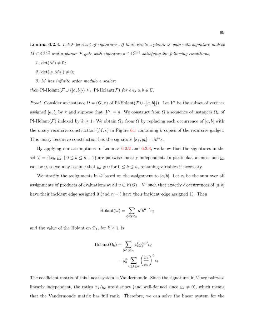
99

Lemma 6.2.4. Let F be a set of signatures. If there exists a planar F-gate with signature matrix

M ∈ C2×2 and a planar F-gate with signature s ∈ C2×1 satisfying the following conditions,

1. det(M) 6= 0;

2. det([s Ms]) 6= 0;

3. M has infinite order modulo a scalar;

then Pl-Holant(F ∪ [a, b]) ≤T Pl-Holant(F) for any a, b ∈ C.

Proof. Consider an instance Ω = (G, π) of Pl-Holant(F ∪ [a, b]). Let V ′ be the subset of vertices

assigned [a, b] by π and suppose that |V ′| = n. We construct from Ω a sequence of instances Ωk of

Pl-Holant(F) indexed by k ≥ 1. We obtain Ωk from Ω by replacing each occurrence of [a, b] with

the unary recursive construction (M, s) in Figure 6.1 containing k copies of the recursive gadget.

This unary recursive construction has the signature [xk, yk] = Mks.

By applying our assumptions to Lemmas 6.2.2 and 6.2.3, we know that the signatures in the

set V = [xk, yk] | 0 ≤ k ≤ n+ 1 are pairwise linearly independent. In particular, at most one yk

can be 0, so we may assume that yk 6= 0 for 0 ≤ k ≤ n, renaming variables if necessary.

We stratify the assignments in Ω based on the assignment to [a, b]. Let c` be the sum over all

assignments of products of evaluations at all v ∈ V (G)−V ′ such that exactly ` occurrences of [a, b]

have their incident edge assigned 0 (and n− ` have their incident edge assigned 1). Then

Holant(Ω) =∑

0≤`≤na`bn−`c`

and the value of the Holant on Ωk, for k ≥ 1, is

Holant(Ωk) =∑

0≤`≤nx`ky

n−`k c`

= ynk∑

0≤`≤n

(xkyk

)`c`.

The coefficient matrix of this linear system is Vandermonde. Since the signatures in V are pairwise

linearly independent, the ratios xk/yk are distinct (and well-defined since yk 6= 0), which means

that the Vandermonde matrix has full rank. Therefore, we can solve the linear system for the

100

N0 N1

N`

N`+1

Figure 6.2: Binary recursive construction with starter gadget used to interpolate[1, 0, 0]. The vertices are assigned [v, 1, 0, 0, 0].

unknown c`’s and obtain the value of Holant(Ω).

The first two conditions of Lemma 6.2.4 are easy to check. The third condition holds in one of

these two cases: either the eigenvalues are the same but M is not a multiple of the identity matrix,

or the eigenvalues are different but their ratio is not a root of unity.

Our refined conditions work well with the anti-gadget technique. The power of this lemma is

that when the third condition fails to hold, there exists an integer k such that Mk = I2, where I2 is

the 2-by-2 identity matrix. Therefore we can construct Mk−1 = M−1 and use this in other gadget

constructions.

6.3 Planar Pairing

In this section, we consider the problem Pl-Holant([v, 1, 0, 0, 0]) when v is different from 0. Over the

next two lemmas, we prove that this problem is #P-hard by reducing from Pl-Holant([v, 1, 0, 0]).

These problems are weighted versions of counting matchings over planar k-regular graphs for k = 4

and k = 3 respectively. The key idea, defined in Definition 6.3.3, is that of a planar pairing.

In the first lemma, we show how to use either the anti-gadget technique or interpolation by

our tight characterization of the unary recursive construction from Section 6.2 to effectively obtain

[1, 0, 0]. The construction in this proof is actually not a unary recursive construction, but a binary

recursive construction. However, degeneracies in the starter and recursive gadgets permit analysis

equivalent to that of the unary recursive construction.

Lemma 6.3.1. For any v ∈ C and signature set F containing [v, 1, 0, 0, 0],

Pl-Holant(F ∪ [1, 0, 0]) ≤T Pl-Holant(F).

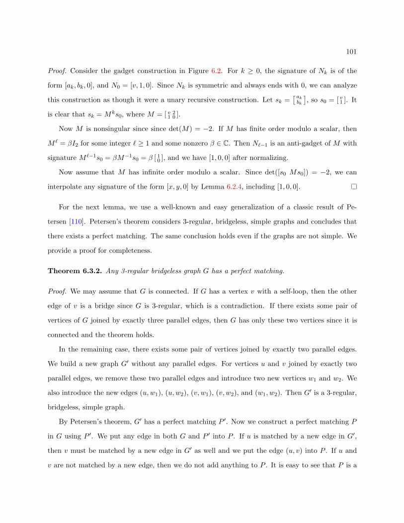
101

Proof. Consider the gadget construction in Figure 6.2. For k ≥ 0, the signature of Nk is of the

form [ak, bk, 0], and N0 = [v, 1, 0]. Since Nk is symmetric and always ends with 0, we can analyze

this construction as though it were a unary recursive construction. Let sk =[ akbk

], so s0 = [ v1 ]. It

is clear that sk = Mks0, where M = [ v 21 0 ].

Now M is nonsingular since since det(M) = −2. If M has finite order modulo a scalar, then

M ` = βI2 for some integer ` ≥ 1 and some nonzero β ∈ C. Then N`−1 is an anti-gadget of M with

signature M `−1s0 = βM−1s0 = β [ 10 ], and we have [1, 0, 0] after normalizing.

Now assume that M has infinite order modulo a scalar. Since det([s0 Ms0]) = −2, we can

interpolate any signature of the form [x, y, 0] by Lemma 6.2.4, including [1, 0, 0].

For the next lemma, we use a well-known and easy generalization of a classic result of Pe-

tersen [110]. Petersen’s theorem considers 3-regular, bridgeless, simple graphs and concludes that

there exists a perfect matching. The same conclusion holds even if the graphs are not simple. We

provide a proof for completeness.

Theorem 6.3.2. Any 3-regular bridgeless graph G has a perfect matching.

Proof. We may assume that G is connected. If G has a vertex v with a self-loop, then the other

edge of v is a bridge since G is 3-regular, which is a contradiction. If there exists some pair of

vertices of G joined by exactly three parallel edges, then G has only these two vertices since it is

connected and the theorem holds.

In the remaining case, there exists some pair of vertices joined by exactly two parallel edges.

We build a new graph G′ without any parallel edges. For vertices u and v joined by exactly two

parallel edges, we remove these two parallel edges and introduce two new vertices w1 and w2. We

also introduce the new edges (u,w1), (u,w2), (v, w1), (v, w2), and (w1, w2). Then G′ is a 3-regular,

bridgeless, simple graph.

By Petersen’s theorem, G′ has a perfect matching P ′. Now we construct a perfect matching P

in G using P ′. We put any edge in both G and P ′ into P . If u is matched by a new edge in G′,

then v must be matched by a new edge in G′ as well and we put the edge (u, v) into P . If u and

v are not matched by a new edge, then we do not add anything to P . It is easy to see that P is a

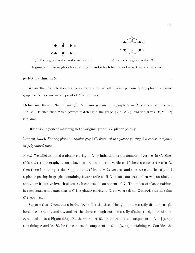
102

u1

v1

u

v

u2

v2

(a) The neighborhood around u and v in G.

u1

v1

u

v

u2

v2

eu

ev

(b) The same neighborhood in H.

Figure 6.3: The neighborhood around u and v both before and after they are removed.

perfect matching in G.

We use this result to show the existence of what we call a planar pairing for any planar 3-regular

graph, which we use in our proof of #P-hardness.

Definition 6.3.3 (Planar pairing). A planar pairing in a graph G = (V,E) is a set of edges

P ⊂ V × V such that P is a perfect matching in the graph (V, V × V ), and the graph (V,E ∪ P )

is planar.

Obviously, a perfect matching in the original graph is a planar pairing.

Lemma 6.3.4. For any planar 3-regular graph G, there exists a planar pairing that can be computed

in polynomial time.

Proof. We efficiently find a planar pairing in G by induction on the number of vertices in G. Since

G is a 3-regular graph, it must have an even number of vertices. If there are no vertices in G,

then there is nothing to do. Suppose that G has n = 2k vertices and that we can efficiently find

a planar pairing in graphs containing fewer vertices. If G is not connected, then we can already

apply our inductive hypothesis on each connected component of G. The union of planar pairings

in each connected component of G is a planar pairing in G, so we are done. Otherwise assume that

G is connected.

Suppose that G contains a bridge (u, v). Let the three (though not necessarily distinct) neigh-

bors of u be v, u1, and u2, and let the three (though not necessarily distinct) neighbors of v be

u, v1, and v2 (see Figure 6.3a). Furthermore, let Hu be the connected component in G − (u, v)

containing u and let Hv be the connected component in G − (u, v) containing v. Consider the

103

induced subgraph H ′u of Hu after adding the edge eu = (u1, u2) (which might be a self-loop on

u = u1 = u2) and then removing u. Similarly, consider the induced subgraph H ′v of Hv after

adding the edge ev = (v1, v2) (which might be a self-loop on v = v1 = v2) and then removing v.

Both H ′u and H ′v are 3-regular graphs and their disjoint union gives a graph H ′ with n−2 = 2(k−1)

vertices (see Figure 6.3b).

By induction on both H ′u and H ′v, we have planar pairings Pu and Pv in H ′u and H ′v respectively.

Let H ′′ be the graph H ′ including the edges Pu∪Pv. If H ′′ contains both eu and ev, then embed H ′′

in the plane so that both eu and ev are adjacent to the outer face. Otherwise, any planar embedding

will do. Then the graph G including the edges Pu ∪ Pv is also planar, so Pu ∪ Pv ∪ (u, v) is a

planar pairing in G.

Otherwise, G is bridgeless. Then by Theorem 6.3.2, G has a perfect matching, which is also

a planar pairing in G. Since a perfect matching can be found in polynomial time by Edmond’s

blossom algorithm [61], the whole procedure is in polynomial time.

After publishing a preliminary version of [74], we realized that a previous construction by Cai

and Kowalczyk uses a planar pairing to show that counting vertex covers over k-regular graphs is

#P-hard for even k ≥ 4 (see the proof of Lemma 15 in [37]). Their algorithm to find a planar

pairing starts by taking a spanning tree and then pairing up the vertices on this tree, which is

simpler than our approach. We believe that it is worth emphasizing the importance of a planar

pairing. Most gadget constructions in hardness proofs for Holant problems are local but the planar

pairing technique is a global argument, which permits reductions that are not otherwise possible.

Now we use the planar pairing technique to show the following.

Lemma 6.3.5. Let v ∈ C. Then Pl-Holant([v, 1, 0, 0]) ≤T Pl-Holant([v, 1, 0, 0, 0]).

Proof. An instance of Pl-Holant([v, 1, 0, 0]) is a signature grid Ω with underlying graph G = (V,E)

that is planar and 3-regular. By Lemma 6.3.4, there exists a planar pairing P in G and it can be

found in polynomial time. Then the graph G′ = (V,E ∪ P ) is planar and 4-regular. We assign

[v, 1, 0, 0, 0] to every vertex in G′. By Lemma 6.3.1, we can assume that we have [1, 0, 0]. We replace

each edge in P with a path of length 2 to form a graph G′′ and assign [1, 0, 0] = [1, 0]⊗2 to each of

104

the new vertices. Then the signature grid Ω′′ with underlying graph G′′ has the same Holant value

as the original signature grid Ω.

Corollary 6.3.6. Let v ∈ C. If v 6= 0, then Pl-Holant([v, 1, 0, 0, 0]) is #P-hard.

Proof. By Lemma 6.3.5, it suffices to show that Pl-Holant([v, 1, 0, 0]) is #P-hard. Then we are

done by applying Theorem 6.1.3, the planar Holant dichotomy for a single ternary signature.

6.4 Counting Eulerian Orientations

Recall the definition of an Eulerian orientation.

Definition 6.4.1. Given a graph G, an orientation of its edges is an Eulerian orientation if for

each vertex v of G, the number of incoming edges of v equals the number of outgoing edges of v.

Counting (unweighted) Eulerian orientations over 4-regular graphs was shown to be #P-hard

in Theorem V.10 of [80]. We improve this result by showing that this problem remains #P-hard

when the graph is also planar. Our reduction is from evaluating the Tutte polynomial of a planar

graph at a point on its diagonal, which have an alternative expression involving medial graphs.

Definition 6.4.2 (cf. [12]). For a connected plane graph G (i.e. a planar embedding of a connected

planar graph), its medial graph H has a vertex for each edge of G and two vertices in H are joined

by an edge for each face of G in which their corresponding edges occur consecutively.

An example of a plane graph and its medial graph are given in Figure 6.4. Any medial graph

is planar and 4-regular. Las Vergnas [136] connected the evaluation of the Tutte polynomial of a

plane graph at the point (3,3) with a sum of weighted Eulerian orientations on its medial graph.

Theorem 6.4.3 (Theorem 2.1 in [136]). Let G be a connected plane graph and let O(Gm) be the

set of all Eulerian orientations in the medial graph Gm of G. Then

2 · Tutte(G; 3, 3) =∑

O∈O(Gm)

2β(O), (6.4.1)

105

(a) (b) (c)

Figure 6.4: A plane graph (a), its medial graph (c), and both graphs superimposed (b).

where β(O) is the number of saddle vertices in the orientation O, i.e. the number of vertices in

which the edges are oriented “in, out, in, out” in cyclic order.

Although the medial graph depends on a particular embedding of the planar graph G, the right

side of (6.4.1) is invariant under different embeddings of G. This follows from (6.4.1) and the fact

that the Tutte polynomial does not depend on the embedding of G.

Now we can prove our hardness result.

Theorem 6.4.4. #Eulerian-Orientations is #P-hard over planar 4-regular graphs.

Proof. We reduce from the right side of (6.4.1) to Pl-Holant(6=2 | [0, 0, 1, 0, 0]), which is the prob-

lem of counting Eulerian orientations over planar 4-regular graphs. Then by Theorem 6.1.4 and

Theorem 6.4.3, we conclude that Pl-Holant(6=2 | [0, 0, 1, 0, 0]) is #P-hard.

The right side of (6.4.1) is the bipartite Holant problem Pl-Holant( 6=2 | f), where

Mf =

0 0 0 1

0 1 2 0

0 2 1 0

1 0 0 0

.

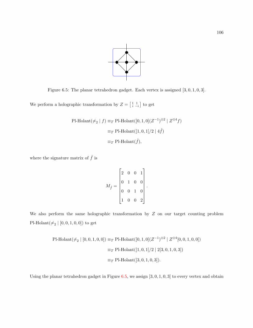
106

Figure 6.5: The planar tetrahedron gadget. Each vertex is assigned [3, 0, 1, 0, 3].

We perform a holographic transformation by Z =[

1 1i −i

]to get

Pl-Holant( 6=2 | f) ≡T Pl-Holant([0, 1, 0](Z−1)⊗2 | Z⊗4f)

≡T Pl-Holant([1, 0, 1]/2 | 4f)

≡T Pl-Holant(f),

where the signature matrix of f is

Mf =

2 0 0 1

0 1 0 0

0 0 1 0

1 0 0 2

.

We also perform the same holographic transformation by Z on our target counting problem

Pl-Holant( 6=2 | [0, 0, 1, 0, 0]) to get

Pl-Holant( 6=2 | [0, 0, 1, 0, 0]) ≡T Pl-Holant([0, 1, 0](Z−1)⊗2 | Z⊗4[0, 0, 1, 0, 0])

≡T Pl-Holant([1, 0, 1]/2 | 2[3, 0, 1, 0, 3])

≡T Pl-Holant([3, 0, 1, 0, 3]).

Using the planar tetrahedron gadget in Figure 6.5, we assign [3, 0, 1, 0, 3] to every vertex and obtain

107

N1 N2

Ns

Ns+1

Figure 6.6: Simple binary recursive construction.

a gadget with signature 32g, where the signature matrix of g is

Mg =1

2

19 0 0 7

0 7 5 0

0 5 7 0

7 0 0 19

.

Now we show how to reduce Pl-Holant(f) to Pl-Holant(g) by interpolation. Consider an instance

Ω of Pl-Holant(f). Suppose that f appears n times in Ω. We construct from Ω a sequence of

instances Ωs of Holant(g) indexed by s ≥ 1. We obtain Ωs from Ω by replacing each occurrence of

f with the gadget Ns in Figure 6.6 with g assigned to all vertices. Since f and g are rotationally

symmetric, it is unnecessary to specify which edge corresponds to which input.

To obtain Ωs from Ω, we effectively replace Mf with MNs = (Mg)s, the sth power of the

signature matrix Mg. Let

T =

0 0 1 1

1 1 0 0

−1 1 0 0

0 0 −1 1

.

Then

Mf = TΛfT−1 = T

1 0 0 0

0 1 0 0

0 0 1 0

0 0 0 3

T−1 and Mg = TΛgT

−1 = T

1 0 0 0

0 6 0 0

0 0 6 0

0 0 0 13

T−1.

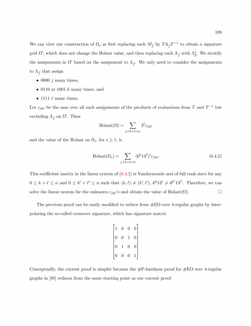
108

We can view our construction of Ωs as first replacing each Mf by TΛfT−1 to obtain a signature

grid Ω′, which does not change the Holant value, and then replacing each Λf with Λsg. We stratify

the assignments in Ω′ based on the assignment to Λf . We only need to consider the assignments

to Λf that assign

• 0000 j many times,

• 0110 or 1001 k many times, and

• 1111 ` many times.

Let cjk` be the sum over all such assignments of the products of evaluations from T and T−1 but

excluding Λf on Ω′. Then

Holant(Ω) =∑

j+k+`=n

3`cjk`

and the value of the Holant on Ωs, for s ≥ 1, is

Holant(Ωs) =∑

j+k+`=n

(6k13`)scjk`. (6.4.2)

This coefficient matrix in the linear system of (6.4.2) is Vandermonde and of full rank since for any

0 ≤ k + ` ≤ n and 0 ≤ k′ + `′ ≤ n such that (k, `) 6= (k′, `′), 6k13` 6= 6k′13`′. Therefore, we can

solve the linear system for the unknown cjk`’s and obtain the value of Holant(Ω).

The previous proof can be easily modified to reduce from #EO over 4-regular graphs by inter-

polating the so-called crossover signature, which has signature matrix

1 0 0 0

0 0 1 0

0 1 0 0

0 0 0 1

Conceptually, the current proof is simpler because the #P-hardness proof for #EO over 4-regular

graphs in [80] reduces from the same starting point as our current proof.

109

6.5 A Demanding Binary Interpolation

Our main result in this chapter is a planar Holant dichotomy for a symmetric signature f of arity 4,

and our main technique to prove the hardness is polynomial interpolation. The binary recursive

construction is a particularly simple construction for which polynomial interpolation is likely to

succeed. To verify the success of this interpolation, we analyze the signature matrix of f . Since f

is symmetric, the signature matrix of f has some redundancies: its second and third rows are the

same and its second and third columns are the same. We “remove” this extra information using

the following definition.

Definition 6.5.1. A 4-by-4 matrix is redundant if its middle two rows and middle two columns

are the same. Denote the set of all redundant 4-by-4 matrices over C by RM4(C).

Consider the function ϕ : C4×4 → C3×3 defined by

ϕ(M) = AMB,

where

A =

1 0 0 0

0 12

12 0

0 0 0 1

and B =

1 0 0

0 1 0

0 1 0

0 0 1

.

Intuitively, the operation ϕ replaces the middle two columns of M with their sum and then the

middle two rows of M with their average. (These two steps commute.) Conversely, we have the

following function ψ : C3×3 → RM4(C) defined by

ψ(N) = BNA.

Intuitively, the operation ψ duplicates the middle row of N and then splits the middle column evenly

into two columns. Notice that ϕ(ψ(N)) = N . When restricted to RM4(C), ϕ is an isomorphism

between the semi-group of 4-by-4 redundant matrices and the semi-group of 3-by-3 matrices, under

110

matrix multiplication, and ψ is its inverse. To see this, just notice that

AB =

1 0 0

0 1 0

0 0 1

and BA =

1 0 0 0

0 12

12 0

0 12

12 0

0 0 0 1

are the identity elements of their respective semi-groups. If the signature matrix Mg of an arity 4

signature g is redundant, we also define the compressed signature matrix of g as Mg = ϕ(Mg).

If all signatures in an F-gate have even arity, then the signature of any F-gate also has even

arity. Knowing that binary signatures alone do not produce #P-hardness, and with the above

constraint in mind, we would like to interpolate another signature of arity 4 using a given signature

of arity 4. We are particularly interested in the signature g with signature matrix

Mg =

1 0 0 0

0 12

12 0

0 12

12 0

0 0 0 1

, (6.5.3)

the identity element in the semi-group of redundant matrices. Thus Mg = I3.

We prove that this signature g is hard. For an asymmetric signature, we often want to reorder

the input bits under a circular permutation. For a single counterclockwise rotation by 90, the

effect on the entries of the signature matrix of an arity 4 signature is given in Figure 3.2.

Lemma 6.5.2. Let g be the arity 4 signature with Mg given in (6.5.3) so that Mg = I3. Then

Pl-Holant(g) is #P-hard.

Proof. We reduce from Pl-Holant(6=2 | [0, 0, 1, 0, 0]), the problem of counting Eulerian orientation

over planar 4-regular graphs, which is #P-hard by Theorem 6.4.4. Recall from the proof of that

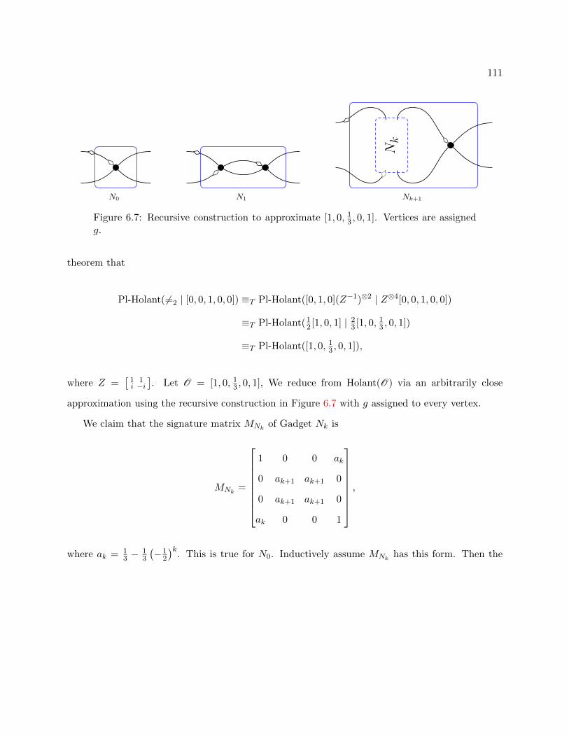
111

N0 N1

Nk

Nk+1

Figure 6.7: Recursive construction to approximate [1, 0, 13 , 0, 1]. Vertices are assigned

g.

theorem that

Pl-Holant( 6=2 | [0, 0, 1, 0, 0]) ≡T Pl-Holant([0, 1, 0](Z−1)⊗2 | Z⊗4[0, 0, 1, 0, 0])

≡T Pl-Holant(12 [1, 0, 1] | 2

3 [1, 0, 13 , 0, 1])

≡T Pl-Holant([1, 0, 13 , 0, 1]),

where Z =[

1 1i −i

]. Let O = [1, 0, 1

3 , 0, 1], We reduce from Holant(O) via an arbitrarily close

approximation using the recursive construction in Figure 6.7 with g assigned to every vertex.

We claim that the signature matrix MNk of Gadget Nk is

MNk =

1 0 0 ak

0 ak+1 ak+1 0

0 ak+1 ak+1 0

ak 0 0 1

,

where ak = 13 −

13

(−1

2

)k. This is true for N0. Inductively assume MNk has this form. Then the

112

rotated form of the signature matrix for Nk, as described in Figure 3.2, is

1 0 0 ak+1

0 ak ak+1 0

0 ak+1 ak 0

ak+1 0 0 1

. (6.5.4)

The action of g on the far right side of Nk+1 is to replace each of the middle two entries in the

middle two rows of the matrix in (6.5.4) with their average, (ak + ak+1)/2 = ak+2. This gives

MNk+1.

Let G be a graph with n vertices and HO (resp. HNk) be the Holant value on G with all vertices

assigned O (resp. Nk). Since each signature entry in O can be expressed as a rational number

with denominator 3, each term in the sum of HO can be expressed as a rational number with

denominator 3n, and HO itself is a sum of 22n such terms, where 2n is the number of edges in G. If

the error |HNk −HO | is at most 1/3n+1, then we can recover HO from HNk by selecting the nearest

rational number to HNk with denominator 3n.

For each signature entry x in MO , its corresponding entry x in MNk satisfies |x − x| ≤ x/2k.

Then for each term t in the Holant sum HO , its corresponding term t in the sum HNk satisfies

t(1 − 1/2k)n ≤ t ≤ t(1 + 1/2k)n, thus −t(1 − (1 − 1/2k)n) ≤ t − t ≤ t((1 + 1/2k)n − 1). Since

1− (1− 1/2k)n ≤ (1 + 1/2k)n − 1, we get |t− t| ≤ t((1 + 1/2k)n − 1). Also each term t ≤ 1. Hence

|HNk −HO | ≤ 22n((

1 + 1/2k)n− 1)< 1/3n+1,

if we take k = 4n.

When I explained this proof to Xi Chen, he thought that it should be possible to prove hardness

using polynomial interpolation instead of this approximation argument. He was right, as I now

demonstrate.

Alternate proof of Lemma 6.5.2. As in the proof of Theorem 6.4.4, we reduce from Pl-Holant(f),

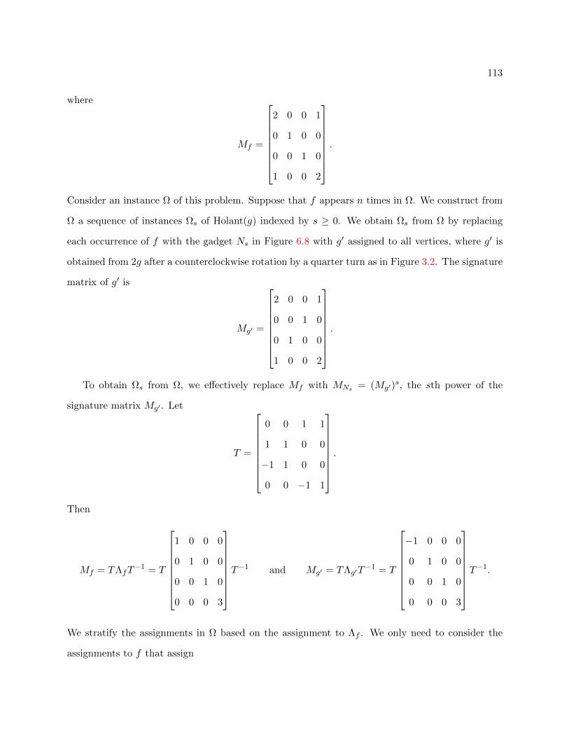
113

where

Mf =

2 0 0 1

0 1 0 0

0 0 1 0

1 0 0 2

.

Consider an instance Ω of this problem. Suppose that f appears n times in Ω. We construct from

Ω a sequence of instances Ωs of Holant(g) indexed by s ≥ 0. We obtain Ωs from Ω by replacing

each occurrence of f with the gadget Ns in Figure 6.8 with g′ assigned to all vertices, where g′ is

obtained from 2g after a counterclockwise rotation by a quarter turn as in Figure 3.2. The signature

matrix of g′ is

Mg′ =

2 0 0 1

0 0 1 0

0 1 0 0

1 0 0 2

.

To obtain Ωs from Ω, we effectively replace Mf with MNs = (Mg′)s, the sth power of the

signature matrix Mg′ . Let

T =

0 0 1 1

1 1 0 0

−1 1 0 0

0 0 −1 1

.

Then

Mf = TΛfT−1 = T

1 0 0 0

0 1 0 0

0 0 1 0

0 0 0 3

T−1 and Mg′ = TΛg′T

−1 = T

−1 0 0 0

0 1 0 0

0 0 1 0

0 0 0 3

T−1.

We stratify the assignments in Ω based on the assignment to Λf . We only need to consider the

assignments to f that assign

114

• 0000 or 0110 or 1001 n− i many times and

• 1111 i many times

since any other assignment contributes a factor of 0. Let ci be the sum over all such assignments

of the products of evaluations from T and T−1 but excluding Λf on Ω. Then

Holant(Ω) =∑

0≤i≤n3ici and Holant(Ωt) =

∑0≤i≤n

9tici

for t = 2s ≥ 0.

Let p(x) =∑

0≤i≤n xici, which has degree at most n with integer coefficients. Using our oracle

for Pl-Holant(g′), we can evaluate this polynomial at n + 1 distinct points x = 9t for 0 ≤ t ≤ n.

Then via polynomial interpolation, we can recover the coefficients of this polynomial efficiently.

Evaluating this polynomial at x = 3 gives the value of Holant(Ω), as desired.

Remark. One advantage of the alternative proof is that it directly reduces from Pl-Holant(f)

instead of going through Pl-Holant([3, 0, 1, 0, 3]). Furthermore, there is no longer a need to give

special attention to Pl-Holant([3, 0, 1, 0, 3]), the problem of counting Eulerian orientations over

planar 4-regular graphs. With this alternative proof, the signature [3, 0, 1, 0, 3] is now swept up by

Lemma 6.5.4 with all the other signatures with redundant and nonsingular compressed signature

matrices.

Most symmetric signatures of arity 4 are hard because they can be used to interpolate the

signature g whose signature matrix is given in (6.5.3). We prove this in Lemma 6.5.4. There are

three cases in Lemma 6.5.4 and one of them requires the following technical lemma.

Lemma 6.5.3. Let M = [B0 B1 · · · Bt] be an n-by-n block matrix such that there exists a λ ∈ C,

for all integers 0 ≤ k ≤ t, block Bk is an n-by-ck matrix for some integer ck ≥ 0, and the entry of

Bk at row r and column c is (Bk)rc = rc−1λkr, where r, c ≥ 1. If λ is nonzero and is not a root of

unity, then M is nonsingular.

Proof. We prove by induction on n. If n = 1, then the sole entry is λk for some nonnegative integer

k. This is nonzero since λ 6= 0. Assume n > 1 and let the left-most nonempty block be Bj . We

115

divide row r by λjr, which is allowed since λ 6= 0. This effectively changes block B` into a block of

the form B`−j . Thus, we have another matrix of the same form as M but with a nonempty block

B0. To simplify notation, we also denote this matrix again by M . The first column of B0 is all 1’s.

We subtract row r − 1 from row r, for r from n down to 2. This gives us a new matrix M ′, and

detM = detM ′. Then detM ′ is the determinant of the (n− 1)-by-(n− 1) submatrix M ′′ obtained

from M ′ by removing the first row and column. Now we do column operations (on M ′′) to return

the blocks to the proper form so that we can invoke the induction hypothesis.

For any block B′k different from B′0, we prove by induction on the number of columns in B′k that

B′k can be repaired. In the base case, the rth element of the first column is (B′k)r1 = λkr−λk(r−1) =

λk(r−1)(λk− 1) for r ≥ 2. We divide this column by λk− 1 to obtain λk(r−1), which is allowed since

λ is not a root of unity and k 6= 0. This is now the correct form for the rth element of the first

column of a block in M ′′.

Now for the inductive step, assume that the first d− 1 columns of block B′k are in the correct

form to be a block in M ′′. That is, for row index r ≥ 2, which denotes the (r − 1)-th row of M ′′,

the rth element in the first d− 1 columns of B′k have the form (B′k)rc = (r− 1)c−1λk(r−1). The rth

element in column d of B′k currently has the form (B′k)rd = rd−1λkr − (r − 1)d−1λk(r−1). Then we

do column operations

(B′k)rd −d−1∑c=1

(d− 1

c− 1

)(B′k)rc = rd−1λkr − (r − 1)d−1λk(r−1) −

d−1∑c=1

(d− 1

c− 1

)(r − 1)c−1λk(r−1)

= rd−1λkr − rd−1λk(r−1)

= rd−1λk(r−1)(λk − 1)

and divide by (λk − 1) to get rd−1λk(r−1). Once again, this is allowed since λ is not a root of unity

and k 6= 0. Then more (of the same) column operations yield

rd−1λk(r−1)−d−1∑c=1

(d− 1

c− 1

)(r−1)c−1λk(r−1) = λk(r−1)

(rd−1 + (r − 1)d−1 −

d∑c=1

(d− 1

c− 1

)(r − 1)c−1

)

and the term in parentheses is precisely (r− 1)d−1. This gives the correct form for the rth element

116

N1 N2

Ns

Ns+1

Figure 6.8: Recursive construction to interpolate g. The vertices are assigned f .

in column d of B′k in M ′′.

Now we repair the columns in B′0, also by induction on the number of columns. In the base

case, if B′0 only has one column, then there is nothing to prove, since this block has disappeared in

M ′′. Otherwise, (B′0)r2 = r − (r − 1) = 1, so the second column is already in the correct form to

be the first column in M ′′, and there is still nothing to prove. For the inductive step, assume that

columns 2 to d− 1 are in the correct form to be the first block in M ′′ for d ≥ 3. That is, the entry

at row r ≥ 2 and column c from 2 through d− 1 has the form (B′0)rc = (r− 1)c−2. The rth element

in column d currently has the form (B′0)rd = rd−1− (r− 1)d−1. Then we do the column operations

(B′0)rd −d−1∑c=2

(d− 1

c− 2

)(B′0)rc = rd−1 − (r − 1)d−1 −

d−1∑c=2

(d− 1

c− 2

)(r − 1)c−2

= (d− 1)(r − 1)d−2

and divide by d − 1, which is nonzero, to get (r − 1)d−2. This is the correct form for the rth

element in column d of B′0 in M ′′. Therefore, we invoke our original induction hypothesis that the

(n− 1)-by-(n− 1) matrix M ′′ has a nonzero determinant, which completes the proof.

Remark. The previous proof is similar to (but more complicated than) the derivation for the

determinant of a Vandermonde matrix.

Lemma 6.5.4. Let f be a signature of arity 4 with complex weights. If Mf is redundant and Mf

is nonsingular, then Pl-Holant(f) is #P-hard.

Proof. Let g be the arity 4 signature with Mg given in (6.5.3). We reduce from Pl-Holant(F ∪g),

which is #P-hard by Lemma 6.5.2.

117

Consider an instance Ω of Pl-Holant(F ∪ g). Suppose that g appears n times in Ω. We

construct from Ω a sequence of instances Ωs of Pl-Holant(F) indexed by s ≥ 1. We obtain Ωs from

Ω by replacing each occurrence of g with the gadget Ns in Figure 6.8 with f assigned to all vertices.

In Ωs, the edge corresponding to the ith significant index bit of Ns connects to the same location

as the edge corresponding to the ith significant index bit of g in Ω.

Now to determine the relationship between Holant(Ω) and Holant(Ωs), we use the isomorphism

between redundant 4-by-4 matrices and 3-by-3 matrices. To obtain Ωs from Ω, we effectively replace

Mg with MNs = (Mf )s, the sth power of the signature matrix Mf . By the Jordan normal form of

Mf , there exist T,Λ ∈ C3×3 such that

Mf = TΛT−1 = T

λ1 b1 0

0 λ2 b2

0 0 λ3

T−1,

where b1, b2 ∈ 0, 1. Note that λ1λ2λ3 = det(Mf ) 6= 0. Also since Mg = ϕ(Mg) = I3, and

TI3T−1 = I3, we have ψ(T )Mgψ(T−1) = Mg. We can view our construction of Ωs as first replacing

each Mg by ψ(T )Mgψ(T−1), which does not change the Holant value, and then replacing each new

Mg with ψ(Λs) = ψ(Λ)s to obtain Ωs. Observe that

ϕ(ψ(T )ψ(Λs)ψ(T−1)) = TΛsT−1 = (Mf )s = (ϕ(Mf ))s = ϕ((Mf )s),

hence, ψ(T )ψ(Λs)ψ(T−1) = MNs . (Since Mg = ψ(T )Mgψ(T−1) and MNs = ψ(T )ψ(Λs)ψ(T−1),

replacing each Mg, sandwiched between ψ(T ) and ψ(T−1), by ψ(Λs) indeed transforms Ω to Ωs.

We also note that, by the isomorphism, ψ(T−1) is the multiplicative inverse of ψ(T ) within the

semi-group of redundant 4-by-4 matrices; but we prefer not to write it as ψ(T )−1 since it is not the

usual matrix inverse as a 4-by-4 matrix. Indeed, ψ(T ) is not invertible as a 4-by-4 matrix.)

In the case analysis below, we stratify the assignments in Ωs based on the assignment to ψ(Λs).

The inputs to ψ(Λs) are from 0, 12 × 0, 12. However, we can combine the input 01 and 10,

since ψ(Λs) is redundant. Thus we actually stratify the assignments in Ωs based on the assign-

118

ment to Λs, which takes inputs from 0, 1, 2 × 0, 1, 2. In this compressed form, the row and

column assignments to Λs are the Hamming weight of the two actual binary valued inputs to the

uncompressed form ψ(Λs).

Now we begin the case analysis on the values of b1 and b2.

1. Assume b1 = b2 = 0. We only need to consider the assignments to Λs that assign

• (0, 0) i many times,

• (1, 1) j many times, and

• (2, 2) k many times

since any other assignment contributes a factor of 0. Let cijk be the sum over all such

assignments of the products of evaluations of all signatures in Ωs except for Λs (including

the contributions from T and T−1). Note that this quantity is the same in Ω as in Ωs. In

particular it does not depend on s. Then

Holant(Ω) =∑

i+j+k=n

cijk2j

and the value of the Holant on Ωs, for s ≥ 1, is

Holant(Ωs) =∑

i+j+k=n

(λi1λ

j2λ

k3

)s (cijk2j

).

The coefficient matrix is Vandermonde, but it may not have full rank because it might be that

λi1λj2λ

k3 = λi

′1λ

j′

2 λk′3 for some (i, j, k) 6= (i′, j′, k′), where i+ j + k = i′ + j′ + k′ = n. However,

this is not a problem since we are only interested in the sum∑ cijk

2j. If two coefficients are

the same, we replace their corresponding unknowns cijk/2j and ci′j′k′/2

j′ with their sum as

a new variable. After all such combinations, we have a Vandermonde system of full rank. In

particular, none of the entries are 0 since λ1λ2λ3 = det(Mf ) 6= 0. Therefore, we can solve the

linear system and obtain the value of Holant(Ω).

2. Assume b1 6= b2. We can permute the Jordan blocks in Λ so that b1 = 1 and b2 = 0, then

λ1 = λ2, denoted by λ. We only need to consider the assignments to Λs that assign

• (0, 0) i many times,

119

• (1, 1) j many times,

• (2, 2) k many times, and

• (0, 1) ` many times

since any other assignment contributes a factor of 0. Let cijk` be the sum over all such

assignments of the products of evaluations of all signatures in Ωs except for Λs (including the

contributions from T and T−1). Then

Holant(Ω) =∑

i+j+k=n

cijk0

2j

and the value of the Holant on Ωs, for s ≥ 1, is

Holant(Ωs) =∑

i+j+k+`=n

λ(i+j)sλks3

(sλs−1

)` (cijk`2j+`

)= λns

∑i+j+k+`=n

(λ3

λ

)kss`( cijk`λ`2j+`

).

If λ3/λ is a root of unity, then take a t such that (λ3/λ)t = 1. Then

Holant(Ωst) = λnst∑

i+j+k+`=n

s`(t`cijk`λ`2j+`

).

For s ≥ 1, this gives a coefficient matrix that is Vandermonde. Although this system is not

full rank, we can replace all the unknowns cijk`/2j having i+ j + k = n− ` by their sum to

form new unknowns c′` =∑

i+j+k=n−`cijk`2j

, where 0 ≤ ` ≤ n. The new unknown c′0 is the

Holant of Ω that we seek. The resulting Vandermonde system

Holant(Ωst) = λnstn∑`=0

s`(t`c′`λ`2`

)

has full rank, so we can solve for the new unknowns and obtain the value of Holant(Ω) = c′0.

If λ3/λ is not a root of unity, then we replace all the unknowns cijk`/(λ`2j+`) having i+j = m

with their sum to form new unknowns c′mk`, for any 0 ≤ m, k, ` and m + k + ` = n. The

120

Holant of Ω is now

Holant(Ω) =∑

m+k=n

c′mk0

and the value of the Holant on Ωs is

Holant(Ωs) = λns∑

i+j+k+`=n

(λ3

λ

)kss`( cijk`λ`2j+`

)= λns

∑m+k+`=n

(λ3

λ

)kss`c′mk`.

After a suitable reordering of the columns, the matrix of coefficients satisfies the hypothesis

of Lemma 6.5.3. Therefore, the linear system has full rank. We can solve for the unknowns

and obtain the value of Holant(Ω).

3. Assume b1 = b2 = 1. In this case, we have λ1 = λ2 = λ3, denoted by λ, and we only need to

consider the assignments to Λs that assign

• (0, 0) or (2, 2) i many times,

• (1, 1) j many times,

• (0, 1) k many times,

• (1, 2) ` many times, and

• (0, 2) m many times

since any other assignment contributes a factor of 0. Let cijk`m be the sum over all such

assignments of the products of evaluations of all signatures in Ωs except for Λs (including the

contributions from T and T−1). Then

Holant(Ω) =∑i+j=n

cij000

2j

121

x0,0 x0,1 x0,2 x0,3 x0,4 x0,5 x0,6

x1,0 x1,1 x1,2 x1,3 x1,4 x1,5

x2,0 x2,1 x2,2 x2,3 x2,4

x3,0 x3,1 x3,2 x3,3

x4,0 x4,1 x4,2

x5,0 x5,1

x6,0

Figure 6.9: An example with n = 6 of how to apply update rules (6.5.5) (solid)and (6.5.6) (dashed).

and the value of the Holant on Ωs, for s ≥ 1, is

Holant(Ωs) =∑

i+j+k+`+m=n

λ(i+j)s(sλs−1

)k+` (s(s− 1)λs−2

)m ( cijk`m2j+k+m

)= λns

∑i+j+k+`+m=n

sk+`+m(s− 1)m( cijk`mλk+`+2m2j+k+m

).

We replace all the unknowns cijk`m/(λk+`+2m2j+k+m) having i + j = p and k + ` = q with

their sum to form new unknowns c′pqm, for any 0 ≤ p, q,m and p+ q+m = n. The Holant of

Ω is now c′n00. This new linear system is

Holant(Ωs) = λns∑

p+q+m=n

sq+m(s− 1)mc′pqm

but is still rank deficient. We now index the columns by (q,m), where q ≥ 0, m ≥ 0, and

q+m ≤ n. Correspondingly, we rename the variables xq,m = c′pqm. Note that p = n−q−m is

determined by (q,m). Observe that the column indexed by (q,m) is the sum of the columns

indexed by (q − 1,m) and (q − 2,m + 1) provided q − 2 ≥ 0. Namely, sq+m(s − 1)m =

sq−1+m(s− 1)m + sq−2+m+1(s− 1)m+1. Of course this is only meaningful if q ≥ 2, m ≥ 0 and

122

q +m ≤ n. We write the linear system as

∑q≥0, m≥0, q+m≤n

αq,mxq,m =Holant(Ωs)

λns,

where αq,m = sq+m(s−1)m are the coefficients. Hence αq,mxq,m = αq−1,mxq,m+αq−2,m+1xq,m,

and we define new variables

xq−1,m ← xq,m + xq−1,m (6.5.5)

xq−2,m+1 ← xq,m + xq−2,m+1 (6.5.6)

from q = n − m down to 2 for every 0 ≤ m ≤ n − 2. See Figure 6.9 for an example with

n = 6.

Observe that in each update, the newly defined variables have a decreased index value for

q. A more crucial observation is that the column indexed by (0, 0) is never updated. This is

because, in order to be an updated entry, there must be some q ≥ 2 and m ≥ 0 such that

(q − 1,m) = (0, 0) or (q − 2,m+ 1) = (0, 0), which is clearly impossible. Hence x0,0 = c′n00 is

still the Holant value on Ω. The 2n+ 1 unknowns that remain are

x0,0, x1,0, x0,1, x1,1, x0,2, x1,2, . . . , x0,n−1, x1,n−1, x0,n

and their coefficients in row s are

1, s, s(s− 1), s2(s− 1), s2(s− 1)2, . . . , sn−1(s− 1)n−1, sn(s− 1)n−1, sn(s− 1)n.

It is clear that the κ-th entry in this row is a monic polynomial in s of degree κ, where 0 ≤

κ ≤ 2n, and thus sκ is a linear combination of the first κ entries. It follows that the coefficient

matrix is a product of the standard Vandermonde matrix multiplied to its right by an upper

triangular matrix with all 1’s on the diagonal. Therefore, the linear system has full rank. We

can solve for these final unknowns and obtain the value of Holant(Ω) = x0,0 = c′n00.

123

Remark. Given such a long and difficult proof, I think some people might miss the basic idea that

lead us to find it in the first place.

Given a symmetric signature of arity 4, we want to interpolate another signature of arity 4 using

the linear construction in Figure 6.8. Why this construction? Because it is (probably) the simplest

arity 4 recursive construction. And what is the worst that can happen? Every nonzero eigenvalue

is a root of unity. Then this construction only provides us with a finite amount of information, but

the amount of information that we need in order to interpolate grows polynomially with the input

size.

And how bad is it? The signature matrix of a symmetric arity 4 signature has 0 for at least

one eigenvalue. If the other three eigenvalues are 1 (and the corresponding eigenvectors are linearly

independent), then the signature of this signature matrix is the one given in (6.5.3). Is this signature

hard? Yes, but we did not know that until after going through this line of reasoning and then finding

a proof that it is hard.

To simplify the application of Lemma 6.5.4 to a symmetric signature, we state and prove its

restriction to a symmetric signature.

Corollary 6.5.5. For a signature [f0, f1, f2, f3, f4] with complex weights, if there does not exist

a, b, c ∈ C, not all zero, such that afk + bfk+1 + cfk+2 = 0 for all k ∈ 0, 1, 2, then Pl-Holant(f)

is #P-hard.

Proof. If the compressed signature matrix Mf is nonsingular, then Pl-Holant(f) is #P-hard by

Lemma 6.5.4, so assume that the rank of Mf is at most 2. Then we have

a′

f0

f1

f2

+ 2b′

f1

f2

f3

+ c′

f2

f3

f4

=

0

0

0

for some a′, b′, c′ ∈ C, not all zero. Thus, a = a′, b = 2b′, and c = c′ have the desired property.

To make Lemma 6.5.4 more applicable, we show that for an arity 4 signature f , the redundancy

of Mf and the nonsingularity of Mf are invariant under an invertible holographic transformation.

124

Lemma 6.5.6. Let f be a signature of arity 4 with complex weights, T ∈ C2×2 a matrix, and

f = T⊗4f . If Mf is redundant, then Mf is also redundant and det(ϕ(Mf )) = det(ϕ(Mf )) det(T )6.

Proof. Since f = T⊗4f , we can express Mf in terms of Mf and T as

Mf = T⊗2Mf (T ᵀ)⊗2 . (6.5.7)

This can be directly checked. Alternatively, this relation is known (and can also be directly checked)

had we not introduced the flip of the middle two columns, i.e., if the columns were ordered

00, 01, 10, 11 by the last two bits in f and f . Instead, the columns are ordered by 00, 10, 01, 11

in Mf and Mf . Let T = (tij), where row index i and column index j range from 0, 1. Then

T⊗2 = (tijti′j′), with row index ii′ and column index jj′. Let

E =

1 0 0 0

0 0 1 0

0 1 0 0

0 0 0 1

,

then ET⊗2E = T⊗2, i.e., a simultaneous row flip ii′ ↔ i′i and column flip jj′ ↔ j′j keep T⊗2 un-

changed. Then the known relations MfE = T⊗2MfE (T ᵀ)⊗2 and E (T ᵀ)⊗2 E = (T ᵀ)⊗2 imply (6.5.7).

Now X ∈ RM4(C) iff EX = X = XE . Then it follows that Mf ∈ RM4(C) if Mf ∈ RM4(C). For

the two matrices A and B in the definition of ϕ, we note that BA = Mg, where Mg given in (6.5.3)

is the identity element of the semi-group RM4(C). Since Mf ∈ RM4(C), we have BAMf = Mf =

MfBA. Then we have

ϕ(Mf ) = AMfB = A(T⊗2Mf (T ᵀ)⊗2

)B

= (AT⊗2B)(AMfB)(A (T ᵀ)⊗2B) (6.5.8)

= ϕ(T⊗2)ϕ(Mf )ϕ((T ᵀ)⊗2).

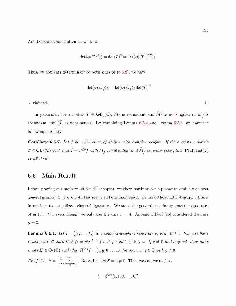
125

Another direct calculation shows that

det(ϕ(T⊗2)) = det(T )3 = det(ϕ((T ᵀ)⊗2)).

Thus, by applying determinant to both sides of (6.5.8), we have

det(ϕ(Mf )) = det(ϕ(Mf )) det(T )6

as claimed.

In particular, for a matrix T ∈ GL2(C), Mf is redundant and Mf is nonsingular iff Mf is

redundant and Mf is nonsingular. By combining Lemma 6.5.4 and Lemma 6.5.6, we have the

following corollary.

Corollary 6.5.7. Let f be a signature of arity 4 with complex weights. If there exists a matrix

T ∈ GL2(C) such that f = T⊗4f with Mf is redundant and Mf is nonsingular, then Pl-Holant(f)

is #P-hard.

6.6 Main Result

Before proving our main result for this chapter, we show hardness for a planar tractable case over

general graphs. To prove both this result and our main result, we use orthogonal holographic trans-

formations to normalize a class of signatures. We state the general case for symmetric signatures

of arity n ≥ 1 even though we only use the case n = 4. Appendix D of [35] considered the case

n = 3.

Lemma 6.6.1. Let f = [f0, . . . , fn] be a complex-weighted signature of arity n ≥ 1. Suppose there

exists c, d ∈ C such that fk = ckαk−1 + dαk for all 1 ≤ k ≤ n. If c 6= 0 and α 6= ±i, then there

exists H ∈ O2(C) such that H⊗nf = [x, y, 0, . . . , 0] for some x, y ∈ C with y 6= 0.

Proof. Let S =

[1 d−1

n

α c+ d−1nα

]. Note that detS = c 6= 0. Then we can write f as

f = S⊗n[1, 1, 0, . . . , 0]ᵀ.

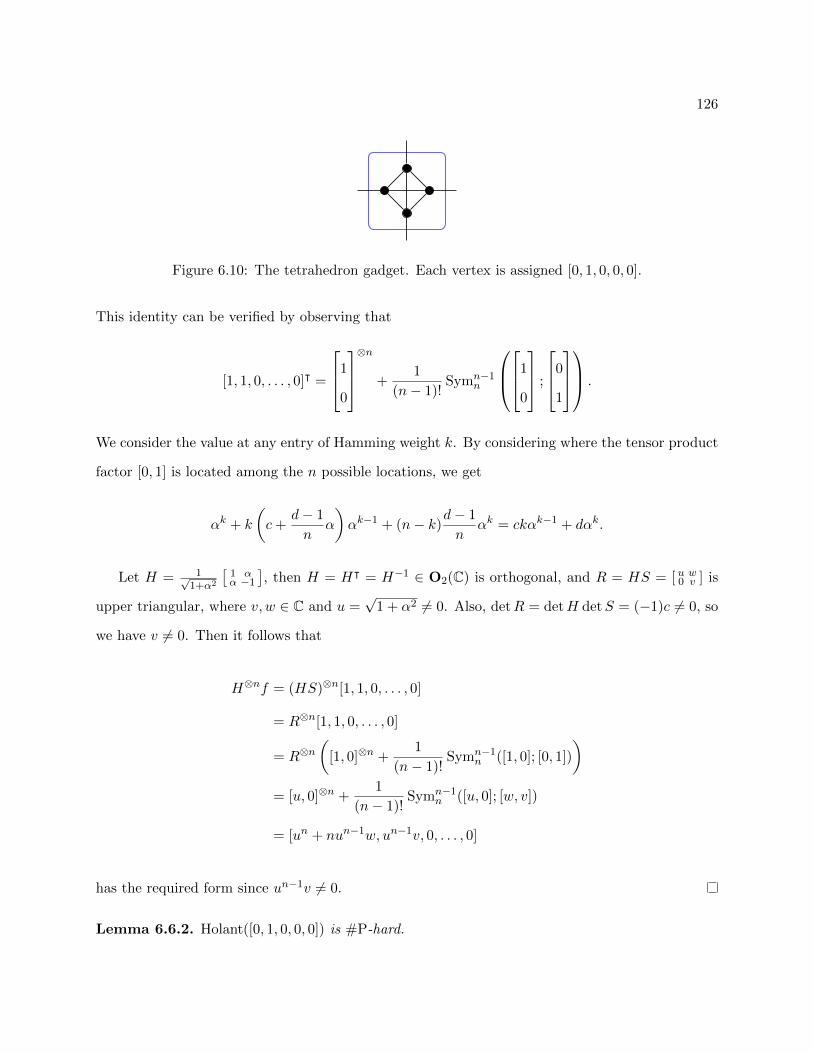
126

Figure 6.10: The tetrahedron gadget. Each vertex is assigned [0, 1, 0, 0, 0].

This identity can be verified by observing that

[1, 1, 0, . . . , 0]ᵀ =

1

0

⊗n

+1

(n− 1)!Symn−1

n

1

0

;

0

1

.

We consider the value at any entry of Hamming weight k. By considering where the tensor product

factor [0, 1] is located among the n possible locations, we get

αk + k

(c+

d− 1

nα

)αk−1 + (n− k)

d− 1

nαk = ckαk−1 + dαk.

Let H = 1√1+α2

[1 αα −1

], then H = Hᵀ = H−1 ∈ O2(C) is orthogonal, and R = HS = [ u w0 v ] is

upper triangular, where v, w ∈ C and u =√

1 + α2 6= 0. Also, detR = detH detS = (−1)c 6= 0, so

we have v 6= 0. Then it follows that

H⊗nf = (HS)⊗n[1, 1, 0, . . . , 0]

= R⊗n[1, 1, 0, . . . , 0]

= R⊗n(

[1, 0]⊗n +1

(n− 1)!Symn−1

n ([1, 0]; [0, 1])

)= [u, 0]⊗n +

1

(n− 1)!Symn−1

n ([u, 0]; [w, v])

= [un + nun−1w, un−1v, 0, . . . , 0]

has the required form since un−1v 6= 0.

Lemma 6.6.2. Holant([0, 1, 0, 0, 0]) is #P-hard.

127

Proof. Consider the gadget in Figure 6.10. We assign [0, 1, 0, 0, 0]) to each vertex. The signature

f of this gadget is f = [3, 0, 1, 0, 1]. The compressed signature matrix of this gadget is nonsingular

since det(Mf ) = 4, so we are done by Lemma 6.5.4.

Now we prove our main result, a planar Holant dichotomy for a symmetric signature of arity 4.

Theorem 6.6.3. If f is a non-degenerate, symmetric, complex-valued signature of arity 4 in

Boolean variables, then Holant(f) is #P-hard unless f is A -transformable or P-transformable

or vanishing, in which case, the problem is computable in polynomial time. If the input is restricted

to planar graphs, then the problem remains #P-hard unless M -transformable, in which case, the

problem is computable in polynomial time.

Proof. Let f = [f0, f1, f2, f3, f4]. If there do not exist a, b, c ∈ C, not all zero, such that for all

k ∈ 0, 1, 2, afk + bfk+1 + cfk+2 = 0, then Pl-Holant(f) is #P-hard by Corollary 6.5.5. Otherwise,

there do exist such a, b, c. If a = c = 0, then b 6= 0, so f1 = f2 = f3 = 0. In this case, f ∈ P is

a generalized equality signature, so f is P-transformable. Now suppose a and c are not both 0.

If b2 − 4ac 6= 0, then there exist α1, α2, β1, β1 ∈ C such that fk = α4−k1 αk2 + β4−k

1 βk2 , where

α1β2 − α2β1 6= 0. A holographic transformation by[α1 β1α2 β2

]transforms f to =4, and we are done

by Theorem 6.1.2. Otherwise, b2−4ac = 0 and there are two cases. In the first, fk = ckαk−1 +dαk

for any 0 ≤ k ≤ 2, where c 6= 0. In the second, fk = c(4− k)α3−k + dα4−k for any 0 ≤ k ≤ 2, where

c 6= 0. These cases map between each other under a holographic transformation by [ 0 11 0 ], so assume

that we are in the first case. If α = ±i, then f is vanishing. Otherwise, there exists an orthogonal

matrix H such that H⊗nf = [x, y, 0, 0, 0] with y 6= 0 by Lemma 6.6.1. Then up to a nonzero factor

of y, we have f = [v, 1, 0, 0, 0], where v = xy . If v 6= 0, then Pl-Holant([v, 1, 0, 0, 0]) is #P-hard

by Corollary 6.3.6. Otherwise v = 0 and the problem is counting perfect matchings over 4-regular

graphs. Thus f ∈ M , so f is M -transformable, and the problem is tractable by Corollary 4.3.7.

Without restricting to planar graphs, Holant([0, 1, 0, 0, 0]) is #P-hard by Lemma 6.6.2.

128

6.7 Closing Thoughts

Superiority of planar pairing Instead of using a planar pairing as was done in the proof of

Lemma 6.3.5, there is another approach that one can try. After explaining this approach though,

I will argue why I believe that planar pairing is a superior proof technique.

The general situation to which planar pairing applies is that every vertex has a dangling edge

and these dangling edges need to be connected together in pairs. To ensure that there are an even

number of dangling edges, we can duplicate the graph [46, Lemma IV.2]. Sometimes multiple

copies are required [81, Lemma 5.4]. In any case though, we solve the resulting problem using an

oracle and want to obtain the solution of the original problem, which is some root of the oracle’s

answer. The question is, which root is the correct one?

The approach used in the works cited above is to

observe that in all the #P-hardness proofs in the current paper and all the #P-hardness

proofs in all the papers on which the current paper depends, when the target Holant

problem for any signature set is proved to be #P-hard, the reduction is from a #P-

complete problem (such as counting vertex covers, matchings, perfect matchings, or

Eulerian orientations), so the solution is a nonnegative integer, and the only three

techniques used in the reduction chains are direct gadget constructions, polynomial

interpolations, and holographic transformations.

The proofs then continue and argue why the unique nonnegative root can be recovered when using

each of these reduction techniques.

The issue with this approach is the difficulty in checking its correctness. One must read all the

#P-hardness proofs in the current paper and all the #P-hardness proofs in all the papers on which

the current paper depends in order to determine if the reductions really are structured as claimed.

This breaks the modularity intended by the use of lemmas, theorems, and the like.1 In contrast,

the technique of planar pairing only requires one to check the correctness of the proof in which it

is used.

1 This type of argument is also used in the proof of Corollary B.5 in [27], but in this instance, the argument isself contained.

129

When the reduction must be planar, the dangling edges must be connected in a planar way.

There are two equally-good ways to accomplish this. In a planar pairing, there must be an even

number of the dangling edges. Then one is able to efficiently pair them up in a planar way.

Alternatively, one can “move” all of the dangling edges to the outer face in some planar embedding

and then pair them up. Moving the dangling edges to the outer face requires the ability to construct

a gadget that functions like as a crossover gadget and allows the dangling edges to move closer to

the outer face. See the proof of Lemma IV.2 in [46] for an example.

130

Chapter 7

Dichotomy for Holant Problems over

General Graphs

We prove a dichotomy theorem for Holant problems over an arbitrary set of complex-valued symmet-

ric constraint functions F on Boolean variables. The dichotomy theorem has an explicit tractability

criterion expressible in terms of holographic transformations. A Holant problem defined by a set

of constraint functions F is solvable in polynomial time if it satisfies this tractability criterion, and

is #P-hard otherwise.

The tractability criterion can be intuitively stated as follows: A set F is tractable if (1) every

function in F has arity at most two, or (2) F is transformable to an affine type, or (3) F is trans-

formable to a product type, or (4) F is vanishing, combined with the right type of binary functions,

or (5) F is highly vanishing, combined with any unary functions. The proof of this theorem utilizes

previous dichotomy theorems for Holant problems and #CSPs. Holographic transformations play

an indispensable role as both a proof technique and in the statement of the tractability criterion.

This work was published in [29, 30].

131

7.1 Background

We prove a dichotomy theorem for Holant problems over an arbitrary set of complex-valued sym-

metric constraint functions F on Boolean variables. Compared to previous dichotomy theorems for

Holant problems, a significant difficultly is the new tractable case of vanishing signatures.

Vanishing signatures are constraint functions, that when applied to any signature grid, produce

a zero Holant value. A simple example is a constraint function of the form (1, i)⊗k on k variables,

which is a tensor product of (1, i). This function on a vertex (of degree k) can be replaced by k

copies of the unary function (1, i) on k new vertices, each connected to an incident edge. Whenever

two copies of (1, i) meet in the Holant sum, they annihilate each other since they give the value

(1, i) · (1, i) = 0.

These ghostly constraint functions are like the elusive dark matter. They do not actually

contribute any value to the Holant sum. However, in order to give a complete dichotomy for

Holant problems, it turns out to be essential that we capture these vanishing signatures. There is

another similarity with dark matter. Their contribution to the Holant sum is not directly observed.

Yet in terms of the dimension of the algebraic variety they constitute, they make up the vast

majority of the tractable symmetric signatures. Furthermore, when combined with others, they

provide a large substrate to produce non-vanishing yet tractable signatures. In #CSP, they are

invisible due to the presumed inclusion of all the Equality functions; and they lurk beneath the

surface when one only considers real-valued Holant problems.

The existence of vanishing signatures have influenced previous dichotomy results, although this

influence was not fully recognized at the time. In the dichotomy theorems in [47] and [35], almost

all tractable signatures can be transformed into a tractable #CSP problem, except for one special

category. The tractability proof for this category used the fact that they are a special case of

generalized Fibonacci signatures [52]. However, what went completely unnoticed is that for every

input instance using such signatures alone, the Holant value is always zero!

The most significant previous encounter with vanishing signatures was in the parity setting [72].

The authors noticed that a large fraction of signatures always induce an even Holant value, which is

vanishing in Z2. However, the parity dichotomy was achieved using an existential argument without

132

obtaining a complete characterization of the vanishing signatures. Consequently, the dichotomy

criterion is non-constructive and is currently not known to be decidable. Nevertheless, this work is

important because it was the first to discover nontrivial vanishing signatures in the parity setting

and to obtain a dichotomy that was completed by vanishing signatures.

We characterize the set of A - and P-transformable signatures after an orthogonal holographic

transformation. An orthogonal transformation is natural since the binary Equality =2 is un-

changed under such a transformation. With explicit characterizations of these tractable signatures,

a complete dichotomy theorem becomes possible. We first prove a dichotomy for a single signa-

ture, and then we extend it to an arbitrary set of signatures. The most difficult part is proving a

dichotomy for a single signature of arity 4, which we did in Chapter 6 and is given in Theorem 6.6.3.

With this dichotomy, we come to a conclusion on a long series of dichotomies on Holant prob-

lems [50, 47, 48, 91, 93, 37, 36, 35, 80]. In particular, this dichotomy extends the dichotomy in [80]

that covers all real-valued symmetric signatures. While we do not rely on their real-valued di-

chotomy itself, we do make important use of one result in [80]: a dichotomy for #CSPd. Recall

that Tk =

[ 1 00 ω ] ∈ C2×2 | ωk = 1

.

Theorem 7.1.1 (Theorem IV.1 in [80]). Let d ≥ 1 be an integer. Suppose F is a set of symmetric,

complex-valued signatures in Boolean variables. Then #CSPd(F) is #P-hard unless F ⊆ P or

∃T ∈ T4d such that F ⊆ TA , in which case the problem is computable in polynomial time.

7.2 Statement of Main Result

Here is the main result of this chapter. The sets V σ and Rσ2 are defined in Section 4.4.

Theorem 7.2.1. Let F be any set of symmetric, complex-valued signatures in Boolean variables.

Then Holant(F) is #P-hard unless F satisfies one of the following conditions, in which case the

problem is computable in polynomial time:

1. All non-degenerate signatures in F are of arity at most 2;

2. F is A -transformable;

3. F is P-transformable;

133

4. F ⊆ V σ ∪ f ∈ Rσ2 | arity(f) = 2 for σ ∈ +,−;

5. All non-degenerate signatures in F are in Rσ2 for σ ∈ +,−.

Note that any signature in Rσ2 having arity at least 3 is a vanishing signature. Thus all signatures

of arity at least 3 in case 5 are vanishing. While both cases 4 and 5 are largely concerned with

vanishing signatures, these two cases differ. In case 4, all signatures in F , including unary signatures

but excluding binary signatures, must be vanishing of a single type σ; the binary signatures are

only required to be in Rσ2 . In contrast, case 5 has no requirement placed on degenerate signatures

which include all unary signatures. Then all non-degenerate binary signatures are required to be

in Rσ2 . Finally all non-degenerate signatures of arity at least 3 are also required to be in Rσ

2 , which

is a strong form of vanishing; they must have a large vanishing degree of type σ.

Case 5 is actually a known tractable case [52, 49]. Every signature (after replacing all degenerate

signatures with corresponding ones) is a generalized Fibonacci signature withm = σ2i, which means

that every signature [f0, f1, . . . , fn] ∈ F satisfies fk+2 = mfk+1 + fk for 0 ≤ k ≤ n − 2. However,

we present a unified proof of tractability based on vanishing signatures.

7.2.1 Proof of Tractability

For any signature grid Ω, Holant(Ω) is the product of the Holant on each connected component, so

we only need to compute over connected components.

For case 1, after decomposing all degenerate signatures into unary ones, a connected component

of the graph is either a path or a cycle and the Holant can be computed using matrix product and

trace. Case 2 is tractable by Corollary 4.2.7. Case 3 is tractable by Corollary 4.1.6. For case 4, any

binary signature g ∈ Rσ2 has rdσ(g) ≤ 1, and thus vdσ(g) ≥ 1 = arity(g)/2. Any signature f ∈ V σ

has vdσ(f) > arity(f)/2. If F contains a signature f of arity at least 3, then it must belong to V σ.

Then by the combinatorial view, more than half of the unary signatures are [1, σi], so Holant(Ω)

vanishes. On the other hand, if the arity of every signature in F is at most 2, then we have reduced

to case 1.

Now consider case 5. After decomposing all degenerate signatures into unary ones, recursively

absorb any unary signature into its neighboring signature. If it is connected to another unary

134

Arity 3 Arity 4

Vanishing

Theorem 7.5.1

Theorem 7.2.1

A -transformableand

P-transformable

Figure 7.1: Dependency graph of key hardness results for our main dichotomy, Theo-rem 7.2.1. The dashed edge indicates a dependency in terms of techniques rather thanthe result itself. “Arity 3(4)” stands for the arity 3(4) single signature dichotomy. “Van-ishing” (“A -transformable and P-transformable”) stands for the lemmas regardingvanishing (A -transformable and P-transformable) signatures. Not all dependencieson previous dichotomy theorems are shown.

signature, then this produces a global constant factor. If it is connected to a binary signature, then

this creates another unary signature. We observe that if f ∈ Rσ2 has arity(f) ≥ 2, then for any

unary signature u, after connecting f to u, the signature 〈f, u〉 still belongs to Rσ2 . Hence after

recursively absorbing all unary signatures in the above process, we still have a signature grid where

all signatures belong to Rσ2 . Any remaining signature f that has arity at least 3 belongs to V σ

since rdσ(f) ≤ 1 and thus vdσ(f) ≥ arity(f)− 1 > arity(f)/2. Thus we have reduced to case 4.

7.2.2 Outline of Hardness Proof

The hardness proof of our main dichotomy is more complicated. Our first goal is to prove a

dichotomy for a single signature, Theorem 7.5.1. The proof is by induction on the arity of the

signature. The induction is done by taking a self loop, which causes the arity to go down by 2.

Thus, we need two base cases, a dichotomy for an arity 3 signature and a dichotomy for an arity 4

signature. The dichotomy for an arity 3 is given in Theorem 6.1.3. The dichotomy for an arity 4

was proved in Chapter 6 and is given in Theorem 6.6.3. It is a crucial ingredient in our proof of

the full dichotomy. It is not only a base case of the single signature dichotomy but also utilized

135

several times in the inductive step.

We begin our proof by considering what signatures mix with the vanishing signatures to give #P-

hardness. When adding unary or binary signatures, the only possible combinations that maintain

the tractability of the vanishing signatures are as described in cases 4 and 5 in Theorem 7.2.1.

Moreover, combining two vanishing signatures of the opposite type of arity at least 3 implies #P-

hardness. The proof of this last statement uses techniques that are similar to those in the proof of

the arity 4 dichotomy.

Another important piece of the proof is to understand the signatures that are A -transformable

or P-transformable. We obtain new explicit characterizations of these signatures. We use these

characterizations to prove dichotomy theorems for any signature set containing an A - or P-

transformable signature. Unless every signature in the set is A - or P-transformable, the problem

is #P-hard. The proofs of these dichotomy theorems utilize the #CSPd dichotomy.

The main dichotomy, Theorem 7.2.1, depends on Theorem 7.5.1 and the results regarding

vanishing signatures as well as the dichotomies when A - or P-transformable signatures appear.

Figure 7.1 summarizes the dependencies among these results.

7.3 Mixing with Vanishing Signatures

We know that vanishing signatures, which were characterized in Section 4.4, are tractable. Now

we determine what signatures combine with them to give #P-hardness. We begin with unary

signatures and their tensor powers.

Lemma 7.3.1. Let f ∈ V σ be a symmetric signature with rdσ(f) ≥ 2 where σ ∈ +,−. Suppose

v = u⊗m is a symmetric degenerate signature for some unary signature u and some integer m ≥ 1.

If u is not a multiple of [1, σi], then Holant(f, v) is #P-hard.

Proof. We consider σ = + since the other case is similar. Since f ∈ V +, we have arity(f) >

2 rd+(f) ≥ 4, and vd+(f) = arity(f) − rd+(f) > 0. As rd+(f) ≥ 2, f is a nonzero signature. By

Lemma 4.4.14, with zero or more self loops of f , we can construct some f ′ with rd+(f ′) = 2 and

arity n ≥ 5. We can repeatedly apply Lemma 4.4.14, since in each step we reduce the recurrence

136

degree rd+ by exactly one, which remains positive and thus the resulting signature is nonzero.

Being obtained from f by self loops, it remains in V +. The process can be continued. After two

more self loops,

Let t = gcd(m,n − 4). There are integers x and y such that xm + y(n − 4) = t. By replacing

x with x+ z(n− 4) and y with y − zm, for any integer z, we may assume x > 0 and y < 0. Then

if we connect |y| copies of [1, i]⊗(n−4) to x copies of v = u⊗m, we can realize u⊗t. Since u is not

a multiple of [1, i], it follows that 〈u, [1, i]〉 is a nonzero constant. We can realize g = u⊗(n−4) by

putting (n− 4)/t many copies of u⊗t together.

Now connect this g back to f ′. Since the unary u is not a multiple of [1, i], we can directly

verify that g 6∈ R+n−4 and thus rd+(g) = arity(g) = n − 4, and vd+(g) = 0. By Lemma 4.4.13,

we get f ′′ = 〈f ′, g〉 of arity 4 and rd+(f ′′) = 2. One can verify that Holant(f ′′) is #P-hard by

Lemma 6.5.4, by writing f ′′k = ikp(k) for some polynomial p of degree exactly 2. A more revealing

proof of the #P-hardness of Holant(f ′′) is by noticing that this is the problem Holant(=2 | f ′′),

which is equivalent to Holant(6=2 | f ′′) under the holographic transformation Z = 1√2

[1 1i −i

]. By

rd+(f ′′) = 2, the signature f ′′ takes the form [f ′′0, f′′

1, f′′

2, 0, 0], where f ′′2 6= 0. Then we are done

by Corollary 6.5.7 after transforming back to the original setting.

Next we consider binary signatures, but first we prove a simple interpolate result.

Lemma 7.3.2. Let x ∈ C. If x 6= 0, then for any set F containing [x, 1, 0], we have

Holant( 6=2 | F ∪ [v, 1, 0]) ≤T Holant( 6=2 | F)

for any v ∈ C.

Proof. Consider an instance Ω of Holant(6=2 | F ∪ [v, 1, 0]). Suppose that [v, 1, 0] appears n

times in Ω. We stratify the assignments in Ω based on the assignments to [v, 1, 0]. We only need

to consider assignments of Hamming weight 0 and 1 since an assignment of Hamming weight 2

contributes a factor of 0. Let i be the number of Hamming weight 0 assignments to [v, 1, 0] in Ω.

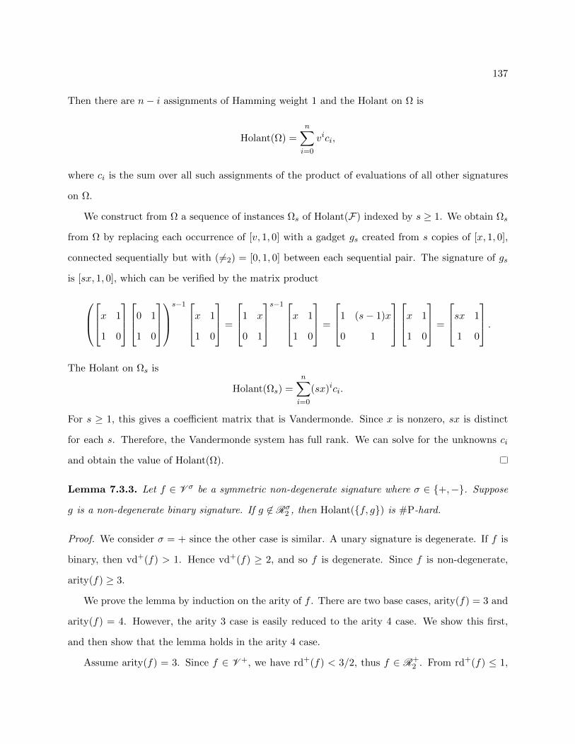
137

Then there are n− i assignments of Hamming weight 1 and the Holant on Ω is

Holant(Ω) =n∑i=0

vici,

where ci is the sum over all such assignments of the product of evaluations of all other signatures

on Ω.

We construct from Ω a sequence of instances Ωs of Holant(F) indexed by s ≥ 1. We obtain Ωs

from Ω by replacing each occurrence of [v, 1, 0] with a gadget gs created from s copies of [x, 1, 0],

connected sequentially but with (6=2) = [0, 1, 0] between each sequential pair. The signature of gs

is [sx, 1, 0], which can be verified by the matrix product

x 1

1 0

0 1

1 0

s−1 x 1

1 0

=

1 x

0 1

s−1 x 1

1 0

=

1 (s− 1)x

0 1

x 1

1 0

=

sx 1

1 0

.The Holant on Ωs is

Holant(Ωs) =n∑i=0

(sx)ici.

For s ≥ 1, this gives a coefficient matrix that is Vandermonde. Since x is nonzero, sx is distinct

for each s. Therefore, the Vandermonde system has full rank. We can solve for the unknowns ci

and obtain the value of Holant(Ω).

Lemma 7.3.3. Let f ∈ V σ be a symmetric non-degenerate signature where σ ∈ +,−. Suppose

g is a non-degenerate binary signature. If g 6∈ Rσ2 , then Holant(f, g) is #P-hard.

Proof. We consider σ = + since the other case is similar. A unary signature is degenerate. If f is

binary, then vd+(f) > 1. Hence vd+(f) ≥ 2, and so f is degenerate. Since f is non-degenerate,

arity(f) ≥ 3.

We prove the lemma by induction on the arity of f . There are two base cases, arity(f) = 3 and

arity(f) = 4. However, the arity 3 case is easily reduced to the arity 4 case. We show this first,

and then show that the lemma holds in the arity 4 case.

Assume arity(f) = 3. Since f ∈ V +, we have rd+(f) < 3/2, thus f ∈ R+2 . From rd+(f) ≤ 1,

138

Figure 7.2: The circles are assigned [t, 1, 0, 0] and the square is assigned 6=2.

we have vd+(f) ≥ 2. On the other hand, f is non-degenerate, so vd+(f) < 3. Thus vd+(f) = 2

and rd+(f) = 1.

We connect two copies of f together by one edge to get an arity 4 signature f ′. By construction,

it may not appear that f ′ is a symmetric signature. However, we show that f ′ is in fact symmetric,

non-degenerate, and vanishing. It is clearly a vanishing signature, since f is vanishing. Consider

the Z transformation, under which f is transformed into f = [t, 1, 0, 0] for some t up to a nonzero

constant. The =2 on the connecting edge between the two copies of f is transformed into 6=2. In

the bipartite setting, our construction is the same as the gadget in Figure 7.2. One can verify that

the resulting signature is f ′ = [2t, 1, 0, 0, 0]. The crucial observation is that it takes the same value

0 on inputs 1010 and 1100, where the left two bits are input to one copy of f and the right two bits

are for another. The corresponding signature f ′ is non-degenerate with rd+(f ′) = 1 and vanishing.

Next we consider the base case of arity(f) = 4. Since f ∈ V +, we have vd+(f) > 2 and

rd+(f) < 2. Since f is non-degenerate, we have rd+(f) 6= −1, 0. Hence rd+(f) = 1 and vd+(f) = 3.

Also by assumption, the given binary g 6∈ R+2 , so we have rd+(g) = 2. Once again, consider the

holographic transformation by Z. This gives

Holant(=2 | f, g) ≡T Holant([1, 0, 1]Z⊗2 | (Z−1)⊗4f, (Z−1)⊗2g)

≡T Holant([0, 1, 0] | f , g),

where up to a nonzero constant, f = [t, 1, 0, 0, 0] and g = [a, b, 1], for some t, a, b ∈ C. We have

a 6= b2 since g is non-degenerate.

Our next goal is to show that we can realize a signature of the form [c, 0, 1] with c 6= 0. If b = 0,

then g is what we want since in this case a = a− b2 6= 0.

Now we assume b 6= 0. By connecting g to f via 6=2, we get [t + 2b, 1, 0]. If t 6= −2b, then

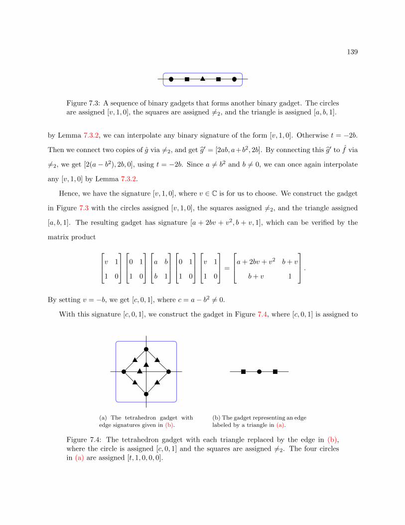
139

Figure 7.3: A sequence of binary gadgets that forms another binary gadget. The circlesare assigned [v, 1, 0], the squares are assigned 6=2, and the triangle is assigned [a, b, 1].

by Lemma 7.3.2, we can interpolate any binary signature of the form [v, 1, 0]. Otherwise t = −2b.

Then we connect two copies of g via 6=2, and get g′ = [2ab, a+b2, 2b]. By connecting this g′ to f via

6=2, we get [2(a− b2), 2b, 0], using t = −2b. Since a 6= b2 and b 6= 0, we can once again interpolate

any [v, 1, 0] by Lemma 7.3.2.

Hence, we have the signature [v, 1, 0], where v ∈ C is for us to choose. We construct the gadget

in Figure 7.3 with the circles assigned [v, 1, 0], the squares assigned 6=2, and the triangle assigned

[a, b, 1]. The resulting gadget has signature [a + 2bv + v2, b + v, 1], which can be verified by the

matrix product

v 1

1 0

0 1

1 0

a b

b 1

0 1

1 0

v 1

1 0

=

a+ 2bv + v2 b+ v

b+ v 1

.By setting v = −b, we get [c, 0, 1], where c = a− b2 6= 0.

With this signature [c, 0, 1], we construct the gadget in Figure 7.4, where [c, 0, 1] is assigned to

(a) The tetrahedron gadget withedge signatures given in (b).

(b) The gadget representing an edgelabeled by a triangle in (a).

Figure 7.4: The tetrahedron gadget with each triangle replaced by the edge in (b),where the circle is assigned [c, 0, 1] and the squares are assigned 6=2. The four circlesin (a) are assigned [t, 1, 0, 0, 0].

140

the circle vertex of arity two in Figure 7.4b and f is assigned to the four circle vertices of arity four

in Figure 7.4a. We get a signature

h = [3c2 + 6ct2 + t4, 3ct+ t3, c+ t2, t, 1].

We note that this computation is reminiscent of matchgate signatures. The internal edge function

[1, 0, c] (which is a flip from [c, 0, 1] since both sides are connected to 6=2) is a generalized equality

signature, and the signature f on the four circle vertices is a weighted version of the matching

function At-Most-One.

The compressed signature matrix of h is

Mh =

3c2 + 6ct2 + t4 2(3ct+ t3) c+ t2

3ct+ t3 2(c+ t2) t

c+ t2 2t 1

and its determinant is 4c3 6= 0. Thus Mh is nonsingular. After a holographic transformation by

Z−1, where Z = 1√2

[1 1i −i

], the binary disequality (6=2) = [0, 1, 0] is transformed to the binary

equality (=2) = [1, 0, 1]. Thus Holant([0, 1, 0] | h) is transformed to Holant(=2 | Z⊗4h), which is

the same as Holant(Z⊗4h). Then we are done by Corollary 6.5.7.

Now we do the induction step. Assume f is of arity n ≥ 5. Since f is non-degenerate, rd+(f) ≥

1. If rd+(f) = 1, then we connect the binary g to f to get f ′ = 〈f, g〉. We have noted that

rd+(g) = 2, so vd+(g) = 0. By Lemma 4.4.13, we have rd+(f ′) = 1 and arity(f ′) = n − 2 ≥ 3.

Thus f ′ is vanishing. Also f ′ is non-degenerate, for otherwise let f ′ = [a, b]⊗(n−2). If [a, b] is a

multiple of [1, i], then rd+(f ′) ≤ 0, which is false. If [a, b] is not a multiple of [1, i], then it can

be directly checked that f ′ 6∈ R+n−2, and rd+(f ′) = n − 2 > 1, which is also false. Hence f ′ is a

non-degenerate vanishing signature of arity n− 2, so we are done by induction hypothesis.

Now suppose rd+(f) = t ≥ 2. Since f is non-degenerate, it is certainly nonzero. Since it is

vanishing, certainly vd+(f) > 0. Hence we can apply Lemma 4.4.14. Let f ′ be obtained from f

by a self loop. Then rd+(f ′) = t − 1 ≥ 1 and arity(f ′) = n − 2. Clearly f ′ is still vanishing.

141

We claim that f ′ is non-degenerate. This follows using the same argument as above. If f ′ were

degenerate, then either rd+(f ′) ≤ 0 or rd+(f ′) = arity(f ′), which would contradict f ′ being a

vanishing signature. Therefore, we can apply the induction hypothesis.

Remark. The gadget in Figure 7.4 is rather complicated. In the process of strengthening this

result to planar graphs [27], we found a simpler proof that Pl-Holant(6=2 | [t, 1, 0, 0, 0], [c, 0, 1]) is

#P-hard provided t 6= 0, which is planar tractable. I give this proof next combined with an equally

simple proof that the Holant( 6=2 | [0, 1, 0, 0, 0], [c, 0, 1]) is #P-hard.

Lemma 7.3.4. Let c, t ∈ C. If c 6= 0, then Holant( 6=2 | [t, 1, 0, 0, 0], [c, 0, 1]) is #P-hard.

Proof. By connecting two copies of 6=2 to either side of [c, 0, 1], we get the signature [1, 0, c] on the

left. Clearly Holant([1, 0, c] | [t, 1, 0, 0, 0]) ≤T Holant( 6=2 | [t, 1, 0, 0, 0], [c, 0, 1]) even when restricted

to planar graphs. Then under a holographic transformation by T−1, where T =[

1 00√c

], we have

Holant([1, 0, c] | [t, 1, 0, 0, 0]) ≡ Holant([1, 0, c](T−1)⊗2 | T⊗4[t, 1, 0, 0, 0])

≡ Holant([1, 0, 1] | [t,√c, 0, 0, 0])

≡ Holant([t,√c, 0, 0, 0])

even when restricted to planar graphs. Up to a nonzero facto of√c, we have Holant([v, 1, 0, 0, 0])

with v = t√c. If v 6= 0, then Pl-Holant([v, 1, 0, 0, 0]) is #P-hard by Corollary 6.3.6. Otherwise t = 0

and Holant([0, 1, 0, 0, 0]) is #P-hard by Lemma 6.6.2.

Next we consider a pair of vanishing signatures of opposite type, both of arity at least 3. We

show that opposite types of vanishing signatures cannot mix. More formally, vanishing signatures

of opposite types, when put together, lead to #P-hardness. First though we show hardness for a

special case.

Lemma 7.3.5. If f = [0, 1, 0, . . . , 0] and g = [0, . . . , 0, 1, 0] are both of arity n ≥ 3, then the problem

Holant([0, 1, 0] | f, g) is #P-hard.

Proof. Our goal is to obtain a signature that satisfies the hypothesis of Corollary 6.5.7.

142

...

(a) The circle is assigned f , the triangle is assignedg, and the squares are assigned 6=2.

(b) The circle is assigned h′, the triangle is as-signed h′′, and the squares are assigned 6=2.

Figure 7.5: Gadget constructions used to obtain a hard and redundant arity 4 signature.

The gadget in Figure 7.5a, with f assigned to the circle vertex, g assigned to the triangle vertex,

and 6=2 assigned to the square vertices, has signature h with signature matrix

Mh =

0 0 0 v

0 1 1 0

0 1 1 0

0 0 0 0

,

where v = n−2 is positive since n ≥ 3. Although this signature matrix is redundant, its compressed

form is singular. Rotating this gadget 90 clockwise and 90 counterclockwise yield signatures h′

and h′′ respectively, with signature matrices

Mh′ =

0 0 0 1

0 v 1 0

0 1 0 0

1 0 0 0

and Mh′′ =

0 0 0 1

0 0 1 0

0 1 v 0

1 0 0 0

.

The gadget in Figure 7.5b, with h′ assigned to the circle vertex, h′′ assigned to the triangle vertex,

and 6=2 assigned to the square vertices, has a signature r with signature matrix

Mr = Mh′

0 0 0 1

0 0 1 0

0 1 0 0

1 0 0 0

Mh′′ =

0 0 0 1

0 v v2 + 1 0

0 1 v 0

1 0 0 0

.

143

N1 N2

Ns

Ns+1

Figure 7.6: Recursive construction to interpolate a signature r′ that is only a rotationaway from having a redundant signature matrix and nonsingular compressed matrix.The circles are assigned r and the squares are assigned 6=2.

Note that the effect of the 6=2 signatures is to reverse all four rows of Mh′′ before multiplying it

to the right of Mh′ . Although this signature matrix is not redundant, every entry of Hamming

weight 2 is nonzero since v is positive.

For any nonzero value t ∈ C, we claim that we can use r to interpolate the following signature

r′ via the construction in Figure 7.6. Define p± = (v ±√v2 + 4)/2, P =

[1 1p+ p−

], and T =

P[t 00 t−1

]P−1 where t ∈ C is any nonzero value. The signature matrix of the target signature r′ is

Mr′ =

0 0 0 1

0T

0

0 0

1 0 0 0

. (7.3.1)

Consider an instance Ω of Holant( 6=2 | F ∪r′) with r ∈ F . Suppose that r′ appears n times in

Ω. We construct from Ω a sequence of instances Ωs of Holant(6=2 | F) indexed by s ≥ 1. We obtain

Ωs from Ω by replacing each occurrence of r′ with the gadget Ns in Figure 7.6 with r assigned to

the circle vertices and 6=2 assigned to the square vertices. In Ωs, the edge corresponding to the

ith significant index bit of Ns connects to the same location as the edge corresponding to the ith

significant index bit of r′ in Ω.

The signature matrix of Ns is the sth power of the matrix obtained from Mr after reversing all

144

rows, and then switching the first and last rows of the final product, namely

0 0 0 1

0 1 0 0

0 0 1 0

1 0 0 0

1 0 0 0

0 1 v 0

0 v v2 + 1 0

0 0 0 1

s

=

0 0 0 1

0 1 v 0

0 v v2 + 1 0

1 0 0 0

1 0 0 0

0 1 v 0

0 v v2 + 1 0

0 0 0 1

s−1

.

The twist of the two input edges on the left side for the first copy of Mr switches the middle two

rows, which is equivalent to a total reversal of all rows, followed by the switching of the first and

last rows. The total reversals of rows for all subsequent s− 1 copies of Mr are due to the presence

of 6=2 signatures.

After such reversals of rows, it is clear that the matrix is a direct sum of block matrices indexed

by 00, 11×00, 11 and 01, 10×10, 01. Furthermore, in the final product, the block indexed

by 00, 11× 00, 11 is [ 0 11 0 ]. Thus in the gadget Ns, the only entries of MNs that vary with s are

the four entries in the middle. These middle four entries of MNs form the 2-by-2 matrix[

1 vv v2+1

]s.

Since[

1 vv v2+1

]= P

[λ+ 00 λ−

]P−1, where λ± = (v2 + 2± v

√v2 + 4)/2 are the eigenvalues, we have

1 v

v v2 + 1

s

= P

λs+ 0

0 λs−

P−1.

The determinant is λ+λ− = 1, so the eigenvalues are nonzero. Since v is positive, the ratio of the

eigenvalues λ+/λ− is not a root of unity, so neither λ+ nor λ− is a root of unity.

Now we determine the relationship between Holant(Ω) and Holant(Ωs). We can view our

construction of Ωs as first replacing Mr′ with

1 0 0 0

0P

0

0 0

0 0 0 1

Λ

1 0 0 0

0P−1

0

0 0

0 0 0 1

=

1 0 0 0

0P

0

0 0

0 0 0 1

0 0 0 1

0 t 0 0

0 0 t−1 0

1 0 0 0

1 0 0 0

0P−1

0

0 0

0 0 0 1

,

145

which does not change the Holant value, and then replacing Λ with

0 0 0 1

0 λs+ 0 0

0 0 λs− 0

1 0 0 0

.

We stratify the assignments in Ωs based on the assignments to the n occurrences of Λ. The

inputs to this matrix are from 0, 12 × 0, 12, which correspond to the four input bits. We only

need to consider the assignments that assign

• i many times the bit pattern 0110,

• j many times the bit pattern 1001, and

• k many times the bit patterns 0011 or 1100,

since any other assignment contributes a factor of 0. Let cijk be the sum over all such assignments

of the products of evaluations of all signatures in Ωs except for Λ. Then

Holant(Ω) =∑

i+j+k=n

ti−jcijk

and the value of the Holant on Ωs, for s ≥ 1, is

Holant(Ωs) =∑

i+j+k=n

λsi+λsj− cijk =

∑i+j+k=n

λs(i−j)+ cijk.

This Vandermonde system does not have full rank. However, we can define for −n ≤ ` ≤ n,

c′` =∑i−j=`

i+j+k=n

cijk.

Then

Holant(Ω) =∑

−n≤`≤nt`c′` and Holant(Ωs) =

∑−n≤`≤n

λs`+c′`.

Now this Vandermonde has full rank because λ+ is neither 0 nor a root of unity. Therefore, we

146

can solve for the unknowns c′` and obtain the value of Holant(Ω). This completes our claim that

we can interpolate the signature r′ in (7.3.1), for any nonzero t ∈ C.

Let t = (√v2 + 8 +

√v2 + 4)/2 so t−1 = (

√v2 + 8−

√v2 + 4)/2. Let a = (

√v2 + 8− v)/2 and

b = (√v2 + 8 + v)/2, so ab = 2 6= 0. One can verify that

P

t 0

0 t−1

P−1 =

a 1

1 b

.Thus, the signature matrix for r′ is

Mr′ =

0 0 0 1

0 a 1 0

0 1 b 0

1 0 0 0

.

After a quarter rotation on the edges of r′, we have a signature r′′ with a redundant signature

matrix

Mr′′ =

0 0 0 a

0 1 1 0

0 1 1 0

b 0 0 0

,

and its compressed signature matrix is nonsingular. After a holographic transformation by Z−1,

where Z = 1√2

[1 1i −i

], the binary disequality (6=2) = [0, 1, 0] is transformed to the binary equality

(=2) = [1, 0, 1]. Thus the problem Holant([0, 1, 0] | r′′) is transformed to Holant(=2 | Z⊗4r′′), which

is the same as Holant(Z⊗4r′′). Then we are done by Corollary 6.5.7.

Lemma 7.3.6. Let f ∈ V + and g ∈ V − be symmetric non-degenerate signatures of arity at least 3.

Then Holant(f, g) is #P-hard.

Proof. Let rd+(f) = d, rd−(g) = d′, arity(f) = n and arity(g) = n′, then 2d < n and 2d′ < n′. We

can apply Lemma 4.4.14 zero or more times to construct a signature obtained from g by adding a

147

certain number of self loops. The resulting signature is a tensor power of [1,−i] up to a nonzero

scalar. To see this, note that we start with rd−(g) < vd−(g) with their sum being arity(g). We

can apply Lemma 4.4.14 if the signature is nonzero and its vd− is positive. Each time we apply

Lemma 4.4.14, we reduce rd− and vd− by one, and the arity by two. Thus rd− < vd− is maintained

until rd− becomes 0, at which point the signature is a tensor power of [1,−i] up to a nonzero scalar.

The initial signature g is non-degenerate by assumption, so it is certainly nonzero. While rd− is

positive, the signature is nonzero, thus Lemma 4.4.14 applies. If d ≥ 2, then by Lemma 7.3.1,

Holant(f, g) is #P-hard. Similarly, the problem is #P-hard if d′ ≥ 2. Thus we may assume that

d = d′ = 1.

We perform the Z = 1√2

[1 1i −i

]transformation

Holant(=2 | f, g) ≡T Holant([1, 0, 1]Z⊗2 | (Z−1)⊗nf, (Z−1)⊗n′g)

≡T Holant([0, 1, 0] | f , g).

Since rd(f) = d = 1, by Lemma 4.4.16, we have (Z−1)⊗nf = f = [f0, f1, 0, . . . , 0], where f1 6= 0.

Similarly, for g with rd−(g) = d′ = 1, we have (Z−1)⊗n′g = g = [0, . . . , 0, g1, g0], where g1 6= 0.

So up to nonzero constants, we have f = [a, 1, 0, . . . , 0] and g = [0, . . . , 0, 1, b] for some a, b ∈ C.

We show that it is always possible to get two such signatures of the same arity minn, n′. Suppose

n > n′. We form a loop from f , where the loop is really a path consisting of one vertex and

two edges, with the vertex assigned the signature 6=2. It is easy to see that this signature is the

degenerate signature 2[1, 0]⊗(n−2). Similarly, we can form a loop from g and can get 2[0, 1]⊗(n′−2).

Thus we have both [1, 0]⊗(n−2) and [0, 1]⊗(n′−2). We can connect all n′ − 2 edges of the second to

the first, connected by 6=2. This gives [1, 0]⊗(n−n′). We can continue subtracting the smaller arity

from the larger one. We continue this process in a subtractive version of the Euclidean algorithm,

and end up with both [1, 0]⊗t and [0, 1]⊗t, where t = gcd(n − 2, n′ − 2) = gcd(n − n′, n′ − 2). In

particular, t | n − n′ and by taking (n − n′)/t many copies of [0, 1]⊗t, we can get [0, 1]⊗(n−n′).

Connecting this back to f via 6=2, we get a symmetric signature of arity n′ consisting of the first

n′ + 1 entries of f . A similar proof works when n′ > n.

148

Thus without loss of generality, we may assume n = n′. If a 6= 0, then connect [0, 1]⊗(n−2)

to f = [a, 1, 0, . . . , 0] via 6=2 we get h = [a, 1, 0]. For a 6= 0, translating this back by Z, we have

a binary signature h 6∈ R−2 together with the given g ∈ V −. By Lemma 7.3.3, Holant(f, g) is

#P-hard. A similar proof works for the case b 6= 0.

The only case left is when f = [0, 1, 0, . . . , 0] of arity n, and g = [0, . . . , 0, 1, 0] of arity n. This

is #P-hard by Lemma 7.3.5.

7.4 A - and P-transformable Signatures

In this section, we investigate the properties of A - and P-transformable signatures. Throughout,

we define α = 1+i√2

=√i = e

πi4 Recall that F123 = F1 ∪ F2 ∪ F3, where F1, F2, and F3 are

defined in Section 4.2. While the main results in this section assume that the signatures involved

are symmetric, we note that some of the lemmas also hold without this assumption.

7.4.1 Characterization of A - and P-transformable Signatures

Recall that by definition, if a set of signatures F is A -transformable (resp. P-transformable),

then the binary equality =2 must be simultaneously transformed into A (resp. P) along with

F . We first characterize the possible matrices of such a transformation by just considering the

transformation of the binary equality. While there are many binary signatures in A ∪P, it turns

out that it is sufficient to consider only three signatures.

Proposition 7.4.1. Let T ∈ C2×2 be a matrix. Then the following hold:

1. [1, 0, 1]T⊗2 = [1, 0, 1] iff T ∈ O2(C);

2. [1, 0, 1]T⊗2 = [1, 0, i] iff there exists an H ∈ O2(C) such that T = H [ 1 00 α ];

3. [1, 0, 1]T⊗2 = [0, 1, 0] iff there exists an H ∈ O2(C) such that T = 1√2H[

1 1i −i

].

Proof. Case 1 is clear since

[1, 0, 1]T⊗2 = [1, 0, 1] ⇐⇒ T ᵀI2T = I2 ⇐⇒ T ᵀT = I2,

the definition of a (2-by-2) orthogonal matrix. Now we use this case to prove the others.

149

For M2 = [ 1 00 α ] and M3 = Z = 1√

2

[1 1i −i

], let Tj = HMj (for j = 2, 3), where H ∈ O2(C). Then

[1, 0, 1]T⊗2j = [1, 0, 1](HMj)

⊗2 = [1, 0, 1]M⊗2j = fj ,

where fj is the binary signature in case j.

On the other hand, suppose that [1, 0, 1](Tj)⊗2 = fj . Then we have

[1, 0, 1](TjM−1j )⊗2 = fj(M

−1j )⊗2 = [1, 0, 1],

so H = TjM−1j ∈ O2(C) by case 1. Thus Tj = HMj as desired.

We also need the following lemma; the proof is direct.

Lemma 7.4.2. If a symmetric signature f = [f0, f1, . . . , fn] can be expressed in the form f =

a[1, λ]⊗n + b[1, µ]⊗n, for some a, b, λ, µ ∈ C, then the fk’s satisfy the recurrence relation fk+2 =

(λ+ µ)fk+1 − λµfk for 0 ≤ k ≤ n− 2.

To simplify the proof of the characterization of the A -transformable signatures, we introduce

the left and right stabilizer groups of A :

LStab(A ) = T ∈ GL2(C) | TA ⊆ A ;

RStab(A ) = T ∈ GL2(C) | A T ⊆ A .

In fact, these two groups are equal and coincide with the group of nonsingular signature matrices

of binary affine signatures. More precisely, for a binary signature f = (f00, f01, f10, f11), we define

its signature matrix Mf to be

Mf =

f00 f01

f10 f11

.Let

A 2×2 = Mf | f ∈ A , arity(f) = 2, and det(Mf ) 6= 0

be the set of nonsingular signature matrices of the binary affine signatures. It is straightforward to

150

verify that A 2×2 is closed under multiplication and inverses. Therefore A 2×2 forms a group.

Let D = [ 1 00 i ] and H2 = 1√

2

[1 11 −1

]. Also let X = [ 0 1

1 0 ] and Z = 1√2

[1 1i −i

]. Note that

Z = DH2 and that D2Z = 1√2

[1 1−i i

]= ZX, hence X = Z−1D2Z. Furthermore, D,H2, X, Z ∈

LStab(A ) ∩ RStab(A ) ∩A 2×2, as well as all nonzero scalar multiples of these matrices.

Not only are the groups LStab(A ), RStab(A ), and A 2×2 equal, they are generated by D and

H2 with a nonzero scalar multiple.

Lemma 7.4.3. LStab(A ) = RStab(A ) = A 2×2 = C∗ · 〈D,H2〉.

Proof. Let

S = S ∈ GL2(C) | F123S ⊆ F123

be the right stabilizer group of F123. It is easy to verify that A 2×2 ⊆ RStab(A ) ⊆ S. Together

with the fact that D,H2 ∈ A 2×2, we have C∗ · 〈D,H2〉 ⊆ A 2×2 ⊆ RStab(A ) ⊆ S. To finish the

proof, we show that S ⊆ C∗ · 〈D,H2〉. For LStab(A ), the proof is similar.

Consider some T ∈ S. For f = (=3), we have fT⊗3 ∈ F123. Then by the form of F123, for

some M ∈ 〈D,H2〉, chosen to be either I, or Hᵀ2 = H2, or Zᵀ = H2D, we have f(TM−1)⊗3 ∈ F1,

which is a generalized equality signature. Then either TM−1 or TM−1X is a diagonal matrix

T ′ = λ[

1 00 d

]. Furthermore, by applying T ′ to =4, we conclude that (=4)T ′⊗4 ∈ F1, since it is in

F123 but not in F2 ∪F3 because T ′ is diagonal. It follows that d is a power of i, and hence[

1 00 d

]is a power of D. Thus T ∈ C∗ · 〈D,H2〉.

Since LStab(A ) = RStab(A ), we simply write Stab(A ) for this group. Of course each T under

which F is A -transformable is just a particular solution that can be extended by any element in

Stab(A ).

Lemma 7.4.4. Let F be a set of signatures. Then F is A -transformable under T iff F is A -

transformable under any T ′ ∈ T Stab(A ).

Proof. Sufficiency is trivial since I2 ∈ Stab(A ). If F is A -transformable under T , then by def-

inition, we have (=2)T⊗2 ∈ A and F ′ = T−1F ⊆ A . Let T ′ = TM ∈ T Stab(A ) for any

M ∈ Stab(A ). It then follows that (=2)T ′⊗2 = (=2)T⊗2M⊗2 ∈ AM = A and T ′−1F = M−1F ′ ⊆

M−1A = A . Therefore F is A -transformable under any T ′ ∈ T Stab(A ).

151

After restricting by Proposition 7.4.1 and normalizing by Lemma 7.4.4, one only needs to check

a small subset of GL2(C) to determine if F is A -transformable.

Lemma 7.4.5. Let F be a set of signatures. Then F is A -transformable iff there exists an

H ∈ O2(C) such that F ⊆ HA or F ⊆ H [ 1 00 α ] A .

Proof. Sufficiency is easily verified by checking that =2 is transformed into A in both cases. In

particular, H leaves =2 unchanged.

If F is A -transformable, then by definition, there exists a matrix T such that (=2)T⊗2 ∈ A

and T−1F ⊆ A . Since =2 is non-degenerate and symmetric, (=2)T⊗2 ∈ A is equivalent to

(=2)T⊗2 ∈ F123.

Any signature in F123 is expressible as c(v⊗n1 + itv⊗n2 ), where t ∈ 0, 1, 2, 3 and (v1, v2) is a

pair of vectors in the set

1

0

,0

1

,

1

1

, 1

−1

,

1

i

, 1

−i

.

We use Stab(A ) to further normalize these three sets by Lemma 7.4.4. In particular, F1 = H2F2

and F1 = (DH2)−1F3. Furthermore, the binary signatures in F1 are just the four signatures

[1, 0, 1], [1, 0, i], [1, 0,−1], and [1, 0,−i] up to a scalar. We also normalize these four as [1, 0, 1] =

[1, 0,−1]D⊗2 and [1, 0, i] = [1, 0,−i]D⊗2. Hence F being A -transformable implies that there exists

a matrix T such that (=2)T⊗2 ∈ [1, 0, 1], [1, 0, i] and T−1F ⊆ A . Now we apply Proposition 7.4.1.

1. If (=2)T⊗2 = [1, 0, 1], then by case 1 of Proposition 7.4.1, we have T ∈ O2(C). Therefore

F ⊆ HA where H = T ∈ O2(C).

2. If (=2)T⊗2 = [1, 0, i], then by case 2 of Proposition 7.4.1, there exists an H ∈ O2(C) such

that T = H [ 1 00 α ]. Therefore F ⊆ TA = H [ 1 0

0 α ] A where H ∈ O2(C).

This completes the proof.

Using these two lemmas, we can characterize all A -transformable signatures. We first define

the three sets A1, A2, and A3.

152

Definition 7.4.6. A symmetric signature f of arity n is in A1 if there exists an H ∈ O2(C) and

a nonzero constant c ∈ C such that f = cH⊗n(

[ 11 ]⊗n

+ β[

1−1

]⊗n), where β = αtn+2r for some

r ∈ 0, 1, 2, 3 and t ∈ 0, 1.

When such an H exists, we say that f ∈ A1 with transformation H. If f ∈ A1 with I2, then

we say f is in the canonical form of A1. If f is in the canonical form of A1, then by Lemma 7.4.2,

for any 0 ≤ k ≤ n− 2, we have fk+2 = fk and one of the following holds:

• f0 = 0, or

• f1 = 0, or

• f1 = ±if0 6= 0, or

• n is odd and f1 = ±(1±√

2)if0 6= 0 (all four sign choices are permissible).

Notice that when n is odd and t = 1 in Definition 7.4.6, it has some complication as described by

the factor αtn+2r.

Definition 7.4.7. A symmetric signature f of arity n is in A2 if there exists an H ∈ O2(C) and

a nonzero constant c ∈ C such that f = cH⊗n(

[ 1i ]⊗n

+[

1−i]⊗n)

.

Similarly, when such an H exists, we say that f ∈ A2 with transformation H. If f ∈ A2 with

I2, then we say f is in the canonical form of A2. If f is in the canonical form of A2, then by

Lemma 7.4.2, for any 0 ≤ k ≤ n− 2, we have fk+2 = −fk. Non-degeneracy of f implies f1 6= ±if0.

It is worth noting that [ 1i ] ,[

1−i] is setwise invariant up to scale under any transformation in

O2(C) up to nonzero constants. That is, these vectors are the eigenvectors of orthogonal matrices.

Thus for any H ∈ O2(C), we can write[

1 1i −i

]−1H[

1 1i −i

]= D, where D is either a diagonal or

anti-diagonal matrix. It is also helpful to view this equation as H[

1 1i −i

]=[

1 1i −i

]D.

Using this fact, the following lemma gives a characterization of A2. It says that any signature

in A2 is essentially in canonical form.

Lemma 7.4.8. Let f be a symmetric arity n signature. Then f ∈ A2 iff f = c(

[ 1i ]⊗n

+ β[

1−i]⊗n)

for some nonzero constants c, β ∈ C.

Proof. Assume f = c(

[ 1i ]⊗n

+ β[

1−i]⊗n)

for some c, β 6= 0. Consider the orthogonal transforma-

tion H =[a bb −a

], where a = 1

2

(β

12n + β−

12n

)and b = 1

2i

(β

12n − β−

12n

). We pick a and b so that

153

a+ bi = β12n , a− bi = β−

12n , and (a+ bi)(a− bi) = a2 + b2 = 1. Also

(a+bia−bi

)n= β. Then

H⊗nf = c

a+ bi

−ai+ b

⊗n

+ β

a− biai+ b

⊗n

= c

(a+ bi)n

1

−i

⊗n

+ (a− bi)nβ

1

i

⊗n

= c√β

1

−i

⊗n

+

1

i

⊗n ,

so f can be written as

f = c√β(H−1)⊗n

1

i

⊗n

+

1

−i

⊗n .

Therefore f ∈ A2.

On the other hand, the desired form f = c([ 1i ]⊗n

+ β[

1−i]⊗n

) follows from the fact that

[ 1i ] ,[

1−i] is fixed setwise under any orthogonal transformation up to nonzero constants.

Definition 7.4.9. A symmetric signature f of arity n is in A3 if there exists an H ∈ O2(C) and

a nonzero constant c ∈ C such that f = cH⊗n(

[ 1α ]⊗n + ir

[1−α]⊗n)

for some r ∈ 0, 1, 2, 3.

Again, when such an H exists, we say that f ∈ A3 with transformation H. If f ∈ A3 with

I2, then we say f is in the canonical form of A3. If f is in the canonical form of A3, then by

Lemma 7.4.2, for any 0 ≤ k ≤ n− 2, we have fk+2 = ifk and one of the following holds:

• f0 = 0, or

• f1 = 0, or

• f1 = ±αif0 6= 0.

Now we characterize the A -transformable signatures.

Lemma 7.4.10. Let f be a non-degenerate symmetric signature. Then f is A -transformable iff

f ∈ A1 ∪A2 ∪A3.

154

Proof. Assume that f is A -transformable of arity n. By applying Lemma 7.4.5 to f, there exists

an H ∈ O2(C) such that f ∈ HA or f ∈ H [ 1 00 α ] A . This is equivalent to (H−1)⊗nf ∈ A or

(H−1)⊗nf ∈ [ 1 00 α ] A . Since f is non-degenerate and symmetric, we can replace A in the previous

expressions with F123. Now we consider the possible cases.

1. If (H−1)⊗nf ∈ F1, then a further transformation by 1√2

[1 11 −1

]∈ O2(C) puts it into the

canonical form of A1.

2. If (H−1)⊗nf ∈ F2, then it is already in the canonical form of A1.

3. If (H−1)⊗nf ∈ F3, then it is already of the equivalent form of A2 given by Lemma 7.4.8.

4. If (H−1)⊗nf ∈ [ 1 00 α ] F1, then a further transformation by 1√

2

[1 11 −1

]∈ O2(C) puts it into the

canonical form of A1.

5. If (H−1)⊗nf ∈ [ 1 00 α ] F2, then it is already in the canonical form of A3.

6. If (H−1)⊗nf ∈ [ 1 00 α ] F3, then it is of the form

[1α3

]⊗n+ ir

[1−α3

]⊗nand a further transfor-

mation by[

0 −11 0

]∈ O2(C) puts it into the canonical form of A3. To see this,

0 −1

1 0

⊗n

1

α3

⊗n

+ ir

1

−α3

⊗n =

−α3

1

⊗n

+ ir

α3

1

⊗n

=(−α3

)n 1

− 1α3

⊗n

+ (−1)nir

1

1α3

⊗n

=(−α3

)n1

α

⊗n

+ i2n+r

1

−α

⊗n .

Let f = H⊗nf be f after the claimed orthogonal transformation. By examining each case

separately, where f is expressed as the sum of two tensor powers, up to a global factor λ 6= 0, the

following forms are possible:

1. f = [ 11 ]⊗n

+ β[

1−1

]⊗nwhere β = αtn+2r for some r ∈ 0, 1, 2, 3 and t ∈ 0, 1 (type A1);

2. f = [ 1i ]⊗n

+ β[

1−i]⊗n

where β = ir (type A2);

3. f = [ 1α ]⊗n + ir

[1−α]⊗n

for some r ∈ 0, 1, 2, 3 (type A3).

Conversely, if there exists a matrix H ∈ O2(C) such that H⊗nf is in one of the canonical

155

forms of A1, A2, or A3, then one can directly check that f is A -transformable. In fact, the

transformations that we applied above are all invertible.

We also have a similar characterization for P-transformable signatures. We define the stabilizer

group of P similar to Stab(A ). It is easy to see the left and right stabilizers coincide, which we

denote by Stab(P). Furthermore, Stab(P) is generated by nonzero scalar multiples of matrices of

the form [ 1 00 ν ] for any nonzero ν ∈ C and X = [ 0 1

1 0 ].

Lemma 7.4.11. Let F be a set of signatures. Then F is P-transformable iff there exists an

H ∈ O2(C) such that F ⊆ HP or F ⊆ H[

1 1i −i

]P.

Proof. Sufficiency is easily verified by checking that =2 is transformed into P in both cases. In

particular, H leaves =2 unchanged.

If F is P-transformable, then by definition, there exists a matrix T such that (=2)T⊗2 ∈ P

and T−1F ⊆ P. The non-degenerate binary signatures in P are either [0, 1, 0] or of the form

[1, 0, ν], up to a scalar. However, notice that [1, 0, 1] = [1, 0, ν][

1 0

0 ν−12

]⊗2and

[1 0

0 ν−12

]∈ Stab(P).

Thus, we only need to consider [1, 0, 1] and [0, 1, 0]. Now we apply Proposition 7.4.1.

1. If (=2)T⊗2 = [1, 0, 1], then by case 1 of Proposition 7.4.1, we have T ∈ O2(C). Therefore

F ⊆ HP where H = T ∈ O(C).

2. If (=2)T⊗2 = [0, 1, 0], then by case 3 of Proposition 7.4.1, there exists an H ∈ O2(C) such

that T = 1√2H[

1 1i −i

]. Therefore F ⊆ H

[1 1i −i

]P where H ∈ O2(C).

We also have similar definitions of the sets P1 and P2.

Definition 7.4.12. A symmetric signature f of arity n is in P1 if there exists H ∈ O2(C) and a

nonzero constant c ∈ C such that f = cH⊗n(

[ 11 ]⊗n

+ β[

1−1

]⊗n), where β 6= 0.

When such an H exists, we say that f ∈ P1 with transformation H. If f ∈ P1 with I2, then

we say f is in the canonical form of P1. If f is in the canonical form of P1, then by Lemma 7.4.2,

for any 0 ≤ k ≤ n− 2, we have fk+2 = fk. Since f is non-degenerate, f1 6= ±f0 is implied.

It is easy to check that A1 ⊂ P1. The corresponding definition for P2 coincides with Defini-

tion 7.4.7 for A2. In other words, we define P2 = A2.

156

Now we characterize the P-transformable signatures as we did for the A -transformable signa-

tures in Lemma 7.4.10.

Lemma 7.4.13. Let f be a non-degenerate symmetric signature. Then f is P-transformable iff

f ∈P1 ∪P2.

Proof. Assume that f is P-transformable of arity n. By applying Lemma 7.4.11 to f, there

exists an H ∈ O2(C) such that f ∈ HP or f ∈ H[

1 1i −i

]P. This is equivalent to (H−1)⊗nf ∈P

or (H−1)⊗nf ∈[

1 1i −i

]P.

The symmetric signatures in P take the form [0, 1, 0], or [a, 0, . . . , 0, b] = a[1, 0]⊗n + b[0, 1]⊗n,

where ab 6= 0 since f is non-degenerate. Now we consider the possible cases.

1. If (H−1)⊗nf =[

101

]= 1

2i

([ 1i ]⊗2 −

[1−i]⊗2)

, then it is already of the equivalent form of

P2 = A2 given by Lemma 7.4.8.

2. If (H−1)⊗nf = a [ 10 ]⊗n

+ b [ 01 ]⊗n

, then a further transformation by 1√2

[1 11 −1

]∈ O2(C) puts

it into the canonical form of P1.

3. If (H−1)⊗nf =[

1 1i −i

]⊗2[

010

]= 2

[101

]=(

[ 11 ]⊗2

+[

1−1

]⊗2)

, then it is already in the canonical

form of P1.

4. If (H−1)⊗nf =[

1 1i −i

]⊗n (a [ 1

0 ]⊗n

+ b [ 01 ]⊗n)

, then it is already of the equivalent form of

P2 = A2 given by Lemma 7.4.8.

Conversely, if there exists a matrix H ∈ O2(C) such that H⊗nf is in one of the canonical forms

of P1 or P2, then one can directly check that f is P-transformable. In fact, the transformations

that we applied above are all invertible.

Combining Lemma 7.4.10 and Lemma 7.4.13, we have a necessary and sufficient condition for

a single non-degenerate signature to be A - or P-transformable.

Corollary 7.4.14. Let f be a non-degenerate signature. Then f is A - or P-transformable iff

f ∈P1 ∪P2 ∪A3.

Notice that our definitions of P1, P2, and A3 each involve an orthogonal transformation. For

any single signature f ∈P1 ∪P2 ∪A3, Holant(f) is tractable. However, this does not imply that

157

Holant(P1), Holant(P2), or Holant(A3) is tractable. One can check, using Theorem 7.2.1, that

Holant(P2) is tractable while Holant(P1) and Holant(A3) are #P-hard.

7.4.2 Dichotomies when A - or P-transformable Signatures Appear

In this subsection, we prove three dichotomies when A - or P-transformable signatures appear.

First though, we prove an interpolation result.

Lemma 7.4.15. Let a, b ∈ C. If ab 6= 0, then for any set F of complex-weighted signatures

containing [a, 0, . . . , 0, b] of arity r ≥ 3,

Holant(F ∪ EQ2) ≤T Holant(F).

The reduction also holds when restricted to planar graphs.

Proof. Since a 6= 0, we can normalize the first entry to get [1, 0, . . . , 0, x], where x 6= 0. First,

we show how to obtain an arity 4 generalized equality signature. If r = 3, then we connect two

copies together by a single edge to get an arity 4 signature. For larger arities, we form self-loops

until realizing a signature of arity 3 or 4. By this process, we have a signature g = [1, 0, 0, 0, y],

where y 6= 0. If y is a pth root of unity, then we can directly realize =4 by connecting p copies of

g together, two edges at a time as in Figure 6.8. Otherwise, y is not a root of unity and we can

interpolate =4 as follows.

Consider an instance Ω of Holant(F∪=4). Suppose that =4 appears n times in Ω. We stratify

the assignments in Ω based on the assignments to =4. We only need to consider the all-zero and

all-one assignments since any other assignment contributes a factor of 0. Let i be the number of

all-one assignments to =4 in Ω. Then there are n− i all-zero assignments and the Holant on Ω is

Holant(Ω) =

n∑i=0

ci,

where ci is the sum over all such assignments of the product of evaluations of all other signatures

on Ω.

158

We construct from Ω a sequence of instances Ωs of Holant(F) indexed by s ≥ 1. We obtain Ωs

from Ω by replacing each occurrence of =4 with a gadget gs created from s copies of [1, 0, 0, 0, y],

connecting two edges together at a time as in Figure 6.8. The Holant on Ωs is

Holant(Ωs) =n∑i=0

(ys)ici.

For s ≥ 1, this gives a coefficient matrix that is Vandermonde. Since y is neither 0 nor a root of

unity, ys is distinct for each s. Therefore, the Vandermonde system has full rank. We can solve for

the unknowns ci and obtain the value of Holant(Ω).

With =4, it is easy to construct all equality signatures of even arity, so we are done.

Our characterizations of A -transformable signatures in Lemma 7.4.10 and P-transformable

signatures in Lemma 7.4.13 are up to transformations in O2(C). Since an orthogonal transformation

never changes the complexity of the problem, in the proofs of following lemmas, we assume any

signature in Ai for i = 1, 2, 3, or Pj for j = 1, 2, is already in the canonical form.

Lemma 7.4.16. Let F be a set of symmetric signatures. Suppose F contains a non-degenerate

signature f ∈ P1 of arity n ≥ 3. Then Holant(F) is #P-hard unless F is P-transformable or

A -transformable.

Proof. By assumption, for any 0 ≤ k ≤ n − 2, fk+2 = fk and f1 6= ±f0 since f is not degenerate.

We can express f as

f = a0

1

1

⊗n

+ a1

1

−1

⊗n

,

where a0 = (f0 + f1)/2 and a1 = (f0 − f1)/2. For this f , we can further perform an orthogonal

transformation by H2 = 1√2

[1 11 −1

]so that f is transformed into the generalized equality signature

2n/2[a0, 0, . . . , 0, a1] of arity n, where a0a1 6= 0. By Lemma 7.4.15, we can realize any equality

signature of even arity. Thus, #CSP2(H2F) ≤T Holant(F).

Now we apply Theorem 7.1.1, the #CSPd dichotomy, to the set H2F . If this problem is #P-

hard, then Holant(F) is #P-hard as well. Otherwise, this problem is #CSP2 tractable. Therefore,

159

there exists some T of the form[

1 00 αk

], where the integer k ∈ 0, 1, . . . , 7, such that TH2F is a

subset of A or P.

If TH2F ⊆ P, then we have H2F ⊆ T−1P. Notice that T ∈ Stab(P), so T−1P = P.

Thus, F is P-transformable under this H2 transformation. Otherwise, TH2F ⊆ A . It is easy

to verify that (=2)((TH2)−1)⊗2 is [1, 0, i−k] ∈ A . Thus, F is A -transformable under this TH2

transformation.

Lemma 7.4.17. Let F be a set of symmetric signatures. Suppose F contains a non-degenerate

signature f ∈ P2 of arity n ≥ 3. Then Holant(F) is #P-hard unless F is P-transformable or

A -transformable.

Proof. By assumption, for any 0 ≤ k ≤ n− 2, fk+2 = −fk and f1 6= ±if0 since f is not degenerate.

We can express f as

f = a0

1

i

⊗n

+ a1

1

−i

⊗n

,

where a0 = (f0 + if1)/2 and a1 = (f0 − if1)/2, and a0a1 6= 0. Then under the holographic

transformation Z ′ =[

n√a0 n

√a1

n√a0i − n

√a1i

]−1, we have

Z ′⊗nf = (=n) =

1

0

⊗n

+

0

1

⊗n

and

Holant(=2 | F ∪ f) ≡T Holant([1, 0, 1](Z ′−1)⊗2 | Z ′F ∪ Z ′⊗nf)

≡T Holant(2a0a1[0, 1, 0] | Z ′F ∪ =n).

Thus, we have a bipartite graph with =n on the right and ( 6=2) = [0, 1, 0] on the left up to a

nonzero scalar, so all equality signatures of arity a multiple of n are realizable on the right side.

To see this, first notice that we can move equality signatures from the right side to the left side

using the binary disequality because the binary disequality just reverses signatures (i.e. exchanges

160

(a) Vertices assigned [1, αi, i,−α]. (b) Vertices assigned [1, αi, i,−α,−1].

Figure 7.7: Constructions to realize [1, 0, i].

the 0 and 1 input bits), which leaves the equality signatures unchanged. Now we do an induction.

Suppose we can realize the equality =(k−1)n on the right side for some integer k > 1. We create

a new signature on the right using one =(k−1)n and two =n on the right and one =n on the left.

Since n ≥ 3, we can connect one wire of the left =n to each of the three equality signatures on

the right. The remaining wires of the left =n can be connected arbitrarily to the signatures on the

right. The resulting signature is an equality of arity (k− 1)n+ 2n−n = kn. Since we have =kn on

both sides for any integer k ≥ 1, #CSPn(Z ′F) ≤T Holant(F).

Now we apply Theorem 7.1.1, the #CSPd dichotomy, to the set Z ′F . If this problem is #P-

hard, then Holant(F) is #P-hard as well. Otherwise, this problem is #CSPn tractable. Let ω be

a primitive 4n-th root of unity. Then under the holographic transformation T =[

1 00 ωk

]for some

integer k, TZ ′F is a subset of A or P. If TZ ′F ⊆ P, then we have Z ′F ⊆ T−1P. Notice that

T ∈ Stab(P), so T−1P = P. Thus, F is P-transformable under this Z ′ transformation.

Otherwise, TZ ′F ⊆ A . It is easy to verify that (=2)((TZ ′)−1)⊗2 is [0, 1, 0] ∈ A up to a scalar.

Thus, F is A -transformable under this TZ ′ transformation.

Lemma 7.4.18. Let F be a set of symmetric signatures. Suppose F contains a non-degenerate

signature f ∈ A3 of arity n ≥ 3. Then Holant(F) is #P-hard unless F is A -transformable.

Proof. By assumption, for any 0 ≤ k ≤ n− 2, we have fk+2 = ifk. We can express f as

f = λ

1

α

⊗n

+ ir

1

−α

⊗n ,

for some integer r.

A self loop on f yields f ′, where f ′k = fk + fk+2 = (1 + i)fk. Thus up to the constant (1 + i),

161

f ′ is just the first n− 2 entries of f . By doing more self loops, we eventually obtain a quaternary

signature when n is even or a ternary one when n is odd. There are eight cases depending on the

first two entries of f and the parity of n. However, for any case, we can realize the signature [1, 0, i].

We list them here. (In the calculations below, we omit certain nonzero constant factors without

explanation.)

• [0, 1, 0, i]: Another self loop gives [0, 1]. Connect it back to the ternary to get [1, 0, i].

• [1, 0, i, 0]: Another self loop gives [1, 0]. Connect it back to the ternary to get [1, 0, i].

• [1, αi, i,−α]: Another self loop gives [1, αi]. Connect two copies of it to the ternary to get

[1,−α]. Then connect this back to the ternary to finally get [1, 0, i]. See Figure 7.7a.

• [1,−αi, i, α]: Same construction as the previous case.

• [0, 1, 0, i, 0]: Another self loop gives [0, 1, 0]. Connect it back to the quaternary to get [1, 0, i].

• [1, 0, i, 0,−1]: Another self loop gives [1, 0, i] directly.

• [1, αi, i,−α,−1]: Another self loop gives [1, αi, i]. Connect two copies of it together to get

[1,−α,−i]. Connect this back to the quaternary to get [1, 0, i]. See Figure 7.7b.

• [1,−αi, i, α,−1]: Same construction as the previous case.

With [1, 0, i] in hand, we can connect three copies to get [1, 0,−i]. Now we construct a bipartite

graph, with F∪=2 on the right side and [1, 0,−i] on the left, and do a holographic transformation

by Z =[α 1−α 1

]to get

Holant([1, 0,−i] | F ∪ f,=2) ≡T Holant([1, 0,−i](Z−1)⊗2 | ZF ∪ Z⊗nf, Z⊗2(=2))

≡T Holant( 12i [1, 0, 1] | ZF ∪ [1, 0, . . . , 0, ik], [1,−i, 1])

≡T Holant(ZF ∪ [1, 0, . . . , 0, ik], [1,−i, 1]

).

Notice that f becomes [1, 0, . . . , 0, ik] where k = r + 2n (after normalizing the first entry) and =2

becomes [1,−i, 1]. On the other side, [1, 0,−i] becomes [1, 0, 1]. By Lemma 7.4.15, we can realize

any equality signature of even arity. Thus, #CSP2(ZF ∪ [1,−i, 1]) ≤T Holant(F).

Now we apply Theorem 7.1.1, the #CSPd dichotomy, to the set ZF∪[1,−i, 1]. If this problem

is #P-hard, then Holant(F) is #P-hard as well. Otherwise, this problem is #CSP2 tractable.

162

Therefore, there exists some T of the form[

1 00 αd

], where the integer d ∈ 0, 1, . . . , 7, such that

TZF ∪ T⊗2[1,−i, 1] is a subset of A or P.

However, T⊗2[1,−i, 1] can never be in P. Thus TZF ∪ T⊗2[1,−i, 1] ⊆ A . Further notice

that if d ∈ 1, 3, 5, 7 in the expression of T , then T⊗2[1,−i, 1] is not in A . Hence, T must be of the

form[

1 00 id

], where the integer d ∈ 0, 1, 2, 3. For such T , T⊗2[1,−i, 1] ∈ A , and T−1A = A as

T ∈ Stab(A ). Thus, TZF∪T⊗2[1,−i, 1] ⊆ A simply becomes ZF ⊆ A . Moreover, (=2)(Z−1)⊗2

is [1, i, 1] ∈ A . Therefore, F is A -transformable under this Z transformation.

7.5 Main Result

In this section, we prove our main dichotomy theorem. We begin with a dichotomy for a single

signature, which we prove by induction on its arity.

Theorem 7.5.1. If f is a non-degenerate symmetric signature of arity at least 3 with complex

weights in Boolean variables, then Holant(f) is #P-hard unless f ∈P1∪P2∪A3 or f is vanishing,

in which case the problem is computable in polynomial time.

Recall that A1 ⊂ P1 and A2 = P2, and f ∈ P1 ∪ P2 ∪ A3 iff f is A -transformable or

P-transformable by Corollary 7.4.14.

Proof. Let the arity of f be n. The base cases of n = 3 and n = 4 are proved in Theorem 6.1.3 and

Theorem 6.6.3 respectively. Now assume n ≥ 5.

With the signature f , we form a self loop to get a signature f ′ of arity at least 3. We consider

the cases separately whether f ′ is degenerate or not.

• Suppose f ′ = [a, b]⊗(n−2) is degenerate. There are three cases to consider.

1. If a = b = 0, then f ′ is the all zero signature. For f , this means fk+2 = −fk for

0 ≤ k ≤ n− 2, so f ∈P2 by Lemma 7.4.8, and therefore Holant(f) is tractable.

2. If a2 + b2 6= 0, then f ′ is nonzero and [a, b] is not a constant multiple of either [1, i] or

[1,−i]. We may normalize so that a2 + b2 = 1. Then the orthogonal transformation[a b−b a

]transforms the column vector [a, b] to [1, 0]. Let f be the transformed signature

from f , and f ′ = [1, 0]⊗(n−2) the transformed signature from f ′.

163

Since an orthogonal transformation keeps =2 invariant, this transformation commutes

with the operation of taking a self loop, i.e., f ′ = (f)′. Here (f)′ is the function obtained

from f by taking a self loop. So f0 + f2 = 1 and for every integer 1 ≤ k ≤ n − 2, we

have fk = −fk+2. With one or more self loops, we eventually obtain either [1, 0] when

n is odd or [1, 0, 0] when n is even. In either case, we connect an appropriate number

of copies of this signature to f to get a arity 4 signature g = [f0, f1, f2,−f1,−f2]. We

show that Holant(g) is #P-hard. To see this, we first compute det(Mg) = −2(f0 +

f2)(f21 + f2

2 ) = −2(f21 + f2

2 ), since f0 + f2 = 1. Therefore if f21 + f2

2 6= 0, Holant(g)

is #P-hard by Lemma 6.5.4. Otherwise f21 + f2

2 = 0, and we consider f2 = if1 since

the other case is similar. Since f is non-degenerate, f is non-degenerate, which implies

f2 6= 0. We can express g as [1, 0]⊗4 − f2[1, i]⊗4. Under the holographic transformation

by T =[

1 (−f2)1/4

0 i(−f2)1/4

], we have

Holant(=2 | g) ≡T Holant([1, 0, 1]T⊗2 | (T−1)⊗4g)

≡T Holant(h | =4),

where

h = [1, 0, 1]T⊗2 = [1, (−f2)1/4, 0]

and g is transformed by T−1 into the arity 4 equality =4, since

T⊗4

1

0

⊗4

+

0

1

⊗4 =

1

0

⊗4

− f2

1

i

⊗4

= g.

By Theorem 6.1.1, Holant(h | =4) is #P-hard as f2 6= 0.

3. If a2 + b2 = 0 but (a, b) 6= (0, 0), then [a, b] is a nonzero multiple of [1,±i]. Ignoring the

constant multiple, we have f ′ = [1, i]⊗(n−2) or [1,−i]⊗(n−2). We consider the first case

since the other case is similar.

In the first case, the characteristic polynomial of the recurrence relation of f ′ is x − i,

164

...

(a) The circles are assigned f and thesquares are assigned 6=2.

...

(b) The circles are assigned f .

Figure 7.8: Two gadgets used when f ′ = [1,±i]⊗(n−2).

so that of f is (x− i)(x2 + 1) = (x− i)2(x+ i). Hence there exist a0, a1, and c such that

fk = (a0 + a1k)ik + c(−i)k

for every integer 0 ≤ k ≤ n. Let f+ and f− be two signatures of arity n such that

f+k = (a0 + a1k)ik and f−k = c(−i)k for every 0 ≤ k ≤ n. Hence fk = f+

k + f−k and we

write f = f+ + f−. If a1 = 0, then f ′ is the all zero signature, a contradiction. If c = 0,

then f is vanishing, one of the tractable cases. Now we assume a1c 6= 0 and show that

Holant(f) is #P-hard. Hence rd+(f+) = 1 and rd−(f−) = 0. Under the holographic

transformation Z = 1√2

[1 1i −i

], we have

Holant(=2 | f) ≡T Holant([1, 0, 1]Z⊗2 | (Z−1)⊗nf)

≡T Holant([0, 1, 0] | f),

where f takes the form [f0, f1, 0, . . . , 0, c′] with c′ = 2n/2c 6= 0 and f1 6= 0, since f is

the Z−1-transformation of the sum of f+ and f−, with rd+(f+) = 1 and rd−(f−) = 0

respectively. On the other side, (=2) = [1, 0, 1] is transformed into ( 6=2) = [0, 1, 0]. Now

consider the gadget in Figure 7.8a with f assigned to both vertices. This gadget has the

binary signature [0, cf0, 2cf1], which is equivalent to [0, f0, 2f1] since c 6= 0. Translating

back by Z to the original setting, this signature is g = [f0 + f1,−if1, f0 − f1]. This can

165

be verified as 1 1

i −i

0 f0

f0 2f1

1 1

i −i

ᵀ

= 2

f0 + f1 −if1

−if1 f0 − f1

.Since f1 6= 0, it can be directly checked that g 6∈ R+

2 .

If f0 6= 0, then g is non-degenerate. In this case we construct some function in V +. We

connect f ′ back to f , getting a binary signature p = Z⊗2[0, 0, c′]. Then we connect p

to f , the resulting signature is p′ = Z⊗n−2[f0, f1, 0, . . . , 0] of arity n − 2 ≥ 3 up to the

constant factor of c′ 6= 0. Notice that p′ is non-degenerate and p′ ∈ V +. By Lemma 7.3.3,

Holant(p′, g) is #P-hard, hence Holant(f) is also #P-hard.

Otherwise suppose f0 = 0. Then we have g = [1,−i]⊗2 after ignoring the nonzero

factor f1. Connecting this degenerate signature to f , we get a signature h = 〈f, g〉.

We note that g annihilates the signature f− = c[1,−i]⊗n, and thus h = 〈f+, g〉. Then

rd+(f+) = 1, vd+(g) = 0, and we can apply Lemma 4.4.13. It follows that rd+(h) = 1

and arity(h) ≥ 3. This implies that h is non-degenerate and h ∈ V +.

Moreover, assigning f to both vertices in the gadget of Figure 7.8b, we get a non-

degenerate signature h′ ∈ V − of arity 4. To see this, consider this gadget after a

holographic transformation by Z. In this bipartite setting, it is the same as assigning

f = [0, f1, 0, . . . , 0, c] (or equivalently [0, 1, 0, . . . , 0, c′′], where c′′ = c/f1 6= 0) to both

the circle and triangle vertices in the gadget of Figure 7.5a. The square vertices there

are still assigned ( 6=2) = [0, 1, 0]. While it is not apparent from the gadget’s geometry,

this signature is in fact symmetric. In particular, its values on inputs 1010 and 1100 are

both 0. The resulting signature is h′ = (Z−1)⊗4h′ = [0, 0, 0, c′′, 0]. Hence rd−(h′) = 1,

and therefore h′ is non-degenerate and h′ ∈ V −.

By Lemma 7.3.6, Holant(h, h′) is #P-hard, hence Holant(f) is also #P-hard.

• Suppose f ′ is non-degenerate. If f ′ is not in one of the tractable cases, then Holant(f ′)

is #P-hard and so is Holant(f). We now assume Holant(f ′) is not #P-hard. Then, by

inductive hypothesis, f ′ ∈ P1 ∪P2 ∪ A3 or f ′ is vanishing. If f ′ ∈ P1 ∪P2 ∪ A3, then

166

applying Lemma 7.4.16, Lemma 7.4.17, or Lemma 7.4.18 to f ′ and the set f, f ′, we either

have that Holant(f, f ′) is #P-hard, so Holant(f) is #P-hard as well, or that f is A - or

P-transformable, so by Corollary 7.4.14, f ∈P1 ∪P2 ∪A3.

Otherwise, f ′ is vanishing, so f ′ ∈ V σ for σ ∈ +,− by Theorem 4.4.12. For simplicity,

assume that f ′ ∈ V +. The other case is similar. Let rd+(f ′) = d−1, where 2d < n and d ≥ 2

since f ′ is non-degenerate. Then the entries of f ′ can be expressed as

f ′k = ikq(k),

where q(x) is a polynomial of degree exactly d − 1. However, notice that if f ′ satisfies

some recurrence relation with characteristic polynomial t(x), then f satisfies a recurrence

relation with characteristic polynomial (x2 + 1)t(x). In this case, t(x) = (x − i)d. Then the

corresponding characteristic polynomial of f is (x− i)d+1(x+ i), and thus the entries of f are

fk = ikp(k) + c(−i)k

for some constant c and a polynomial p(x) of degree at most d. However, the degree of p(x)

is exactly d, otherwise the polynomial q(x) for f ′ would have degree less than d− 1. If c = 0,

then f is vanishing, a tractable case. Otherwise, c 6= 0, and we show the problem is #P-hard.

Under the transformation Z = 1√2

[1 1i −i

], we have

Holant(=2 | f) ≡T Holant([1, 0, 1]Z⊗2 | (Z−1)⊗nf)

≡T Holant([0, 1, 0] | f),

where f = [f0, f1, . . . , fd, 0, . . . , 0, c], with fd 6= 0. Taking a self loop in the original setting

is equivalent to connecting [0, 1, 0] to a signature after this transformation. Thus, doing this

once on f , we can get f ′ = [f1, . . . , fd, 0, . . . , 0] corresponding to f ′, and doing this d−2 times

on f , we get a signature h = [fd−2, fd−1, fd, 0, . . . , 0, 0/c] of arity n − 2(d − 2) = n − 2d + 4.

The last entry is c when d = 2 and is 0 when d > 2.

167

As n > 2d, we may do two more self loops and get [fd, 0, . . . , 0] of arity k = n − 2d. Now

connect this signature back to f via [0, 1, 0]. It is the same as getting the last n−k+1 = 2d+1

signature entries of f . We may repeat this operation zero or more times until the arity k′ of

the resulting signature is less than or equal to k. We claim that this signature has the form

g = [0, . . . , 0, c]. In other words, the k′ + 1 entries of g consist of the last c and k′ many 0’s

in the signature f , all appearing after fd. This is because there are n− d− 1 many 0 entries

in the signature f after fd, and n− d− 1 ≥ k ≥ k′.

Translating back by the Z transformation, having both [fd, 0, . . . , 0] of arity k and g =

[0, . . . , 0, c] of arity k′ is equivalent to, in the original setting, having both [1, i]⊗k and [1,−i]⊗k′ .

If k > k′, then we can connect [1,−i]⊗k′ to [1, i]⊗k and get [1, i]⊗(k−k′). Replacing k by k−k′,

we can repeat this process until the new k ≤ k′. If the new k < k′, then we can continue as in

the subtractive Euclid algorithm. We continue this procedure and eventually we get [1, i]⊗t

and [1,−i]⊗t, where t = gcd(k, k′), where k = n − 2d and k′ ≤ k, as defined in the previous

paragraph. Now putting k/t many copies of [1,−i]⊗t together, we get [1,−i]⊗k.

In the transformed setting, [1,−i]⊗k is [0, . . . , 0, 1] of arity k. Then we connect this back to

h via [0, 1, 0]. Doing this is the same as forcing k connected edges of h to be assigned 0,

because [0, 1, 0] flips the assigned value 1 in [0, . . . , 0, 1] to 0. Thus we get a signature of arity

n − 2d + 4 − k = 4, which is [fd−2, fd−1, fd, 0, 0]. Note that the last entry is 0 (and not c).

Then we are done by Corollary 6.5.7 after transforming back to the original setting.

Now we are ready to prove of our main theorem.

Proof of hardness for Theorem 7.2.1. Assume that Holant(F) is not #P-hard. If all of the non-

degenerate signatures in F are of arity at most 2, then the problem is tractable case 1. Otherwise

we have some non-degenerate signatures of arity at least 3. For any such f , by Theorem 7.5.1,

f ∈ P1 ∪P2 ∪A3 or f is vanishing. If any of them is in P1 ∪P2 ∪A3, then by Lemma 7.4.16,

Lemma 7.4.17, or Lemma 7.4.18, we have that F is A - or P-transformable, which are tractable

cases 2 and 3.

Now we assume that all non-degenerate signatures of arity at least 3 in F are vanishing, and

168

there is a nonempty set of such signatures in F . By Lemma 7.3.6, they must all be in V σ with the

same σ ∈ +,−. By Lemma 7.3.3, we know that any non-degenerate binary signature in F has

to be in Rσ2 . Furthermore, if F contains an f ∈ V σ such that rdσ(f) ≥ 2, then by Lemma 7.3.1,

the only unary signatures allowed in F are some multiple of [1, σi], and all degenerate signatures in

F are a tensor product of some multiple of [1, σi]. Thus, all non-degenerate signatures of arity at

least 3 as well as all degenerate signatures belong to V σ, and all non-degenerate binary signatures

belong to Rσ2 . This is tractable case 4.

Finally, we have the following: (i) all non-degenerate signatures of arity at least 3 in F belong

to V σ; (ii) all signatures f ∈ F ∩ V σ have rdσ(f) ≤ 1, which implies that f ∈ Rσ2 ; and (iii) all

non-degenerate binary signatures in F belong to Rσ2 . Hence all non-degenerate signatures in F

belong to Rσ2 . All unary signatures also belong to Rσ

2 by definition. This is indeed tractable case 5.

The proof is complete.

If F is finite, then the criterion of Theorem 7.2.1 is decidable in polynomial time [31, 34].

7.6 Closing Thoughts

A planar dichotomy implies a nonplanar dichotomy This dichotomy was generalized by

restricting to planar graphs [27]. We were surprised to find new cases that are planar tractable but

not by holographic reductions to matchgates and ultimately the FKT algorithm.

A dichotomy for Pl-Holant(F) implies a dichotomy for Holant(F). This is because Holant(F)

can be viewed as the special case of Pl-Holant(F) when F contains this “crossover signature” X,

which has signature matrix

MX =

1 0 0 0

0 0 1 0

0 1 0 0

0 0 0 1

.

Clearly Pl-Holant(F) ≤T Holant(F). For the other direction, take an instance Ω of Holant(F) and

embed the underlying graph in the plane so that at most two edges cross at any point. At each

169

of these points, add a vertex assigned X to replace these crossed edges. This does not change the

Holant value and is now an instance of Pl-Holant(F) since X ∈ F .

170

Chapter 8

Dichotomy for #CSP over Planar

Graphs

We prove a dichotomy theorem for symmetric complex-weighted Boolean #CSP when the constraint

graph of the input must be planar. The problems that are #P-hard over general graphs but

tractable over planar graphs are precisely those with a holographic reduction to matchgates. This

generalizes a theorem [46] to the case of real weights. The main idea is to use the popular pinning

technique, but because of the planarity restriction, this only possible in the Hadamard basis. This

work was published in [73, 74].

8.1 Background

In 1979, Valiant [125] defined the class #P to explain the apparent intractability of counting perfect

matchings in a graph. Yet over a decade earlier, Kasteleyn [89, 88] gave a polynomial-time algorithm

to compute this quantity for planar graphs. This was an important milestone in a decades-long

research program by physicists in statistical mechanics to determine what problems the restriction

to the planar setting renders tractable [5, 83, 109, 145, 146, 97, 120, 87, 89, 68, 88, 101, 102, 141].

More recently, Valiant introduced matchgates [128, 127] and holographic algorithms [132, 131] that

rely on Kasteleyn’s algorithm to solve certain counting problems over planar graphs. Subsequently,

171

the signatures with holographic transformations to matchgates were characterized (as described in

Section 4.3).

From the viewpoint of computational complexity, we seek to understand exactly which in-

tractable problems the planarity restriction enable us to efficiently compute. Partial answers to

this question have been given in the context of various counting frameworks [138, 36], including

the dichotomy from Chapter 5 and a dichotomy for symmetric complex-weighted Boolean #CSP

in [46]. In every case, the problems that are #P-hard over general graphs but tractable over planar

graphs are essentially those given in Section 4.3. In this chapter, we give more evidence for this

phenomenon by extending the dichotomy in [46] from real to complex weights. This extension also

generalizes the dichotomy in [53] by restricting to planar graphs.

Our main result is stated as follows.

Theorem 8.1.1. Let F be any set of symmetric, complex-valued signatures in Boolean variables.

Then Pl-#CSP(F) is #P-hard unless F satisfies one of the following conditions, in which case it

is tractable:

1. #CSP(F) is tractable (cf. [53]); or

2. F is realizable by matchgates (cf. Section 4.3).

A more explicit description of the tractable cases can be found in Theorem 8.5.3.

Although this theorem is stated for the framework of counting constraint satisfaction problems

(#CSP), our proof is in the more general framework of Holant problems. From the Holant per-

spective, the set EQ = =n | n ≥ 1 of Equality signatures is always available in #CSP(F). By

the signature theory of Cai and Lu [43], the Hadamard matrix H =[

1 11 −1

]defines the only1 holo-

graphic transformation under which EQ becomes matchgate realizable. Let F denote HF for any

set F of signatures. Then EQ = [1, 0], [1, 0, 1], [1, 0, 1, 0], . . . is the set of unweighted signatures

with even support. Therefore, #CSP(F), which is equivalent to Holant(F ∪ EQ) by Lemma 2.2.1,

is further equivalent to Holant(F ∪ EQ) by Lemma 3.2.2.

In many previous dichotomy theorems for Boolean #CSP(F), the proof of hardness began by

pinning. The goal of this technique is to realize the constant functions [1, 0] and [0, 1] and was

1Up to transformations under which matchgates are closed.

172

always achieved by a nonplanar reduction. In the nonplanar setting, [1, 0] and [0, 1] are contained

in each of the maximal tractable sets. Therefore, pinning in this setting does not imply the collapse

of any complexity classes. However, the signatures in EQ ∪ [1, 0], [0, 1] are not simultaneously

realizable by matchgates. If we are to prove our main theorem, one should not expect to be able

to pin for Pl-#CSP(F), since otherwise #P would collapse to P. Instead, apply the Hadamard

transformation and consider Pl-Holant(F ∪EQ). In this Hadamard basis, pinning becomes possible

again since [1, 0] and [0, 1] are included in every maximal tractable set. Indeed, we prove our

pinning result in this Hadamard basis in Section 8.4. The pinned version of Pl-Holant(F ∪ EQ),

which assumes that the signatures [1, 0] and [0, 1] are available, is denoted by Pl-Holantc(F ∪ EQ)

(where c stands for constants).

Our other main technique is domain pairing. This technique is used to overcome a parity

restriction. If all signatures have even arity, then the signature of any gadget will also have even

arity. Domain pairing is a type of reduction that allows us to realize a signature of odd arity given

only signatures of even arity.

We use Theorem 6.1.1 with G = EQ, which is the special case of Pl-#CSP(F) when F contains

a single binary signature. Furthermore, we perform a holographic transformation by the Hadamard

matrix H =[

1 11 −1

]. Under this transformation, it is easy to see that the conditions f0f2 = f2

1 and

f0f2 = −f21 ∧ f0 = −f2 are invariant while the conditions f1 = 0 and f0 = f2 map to each other.

Therefore, by an apparent coincidence, the tractability conditions remain the same. To be clear,

we restate Theorem 6.1.1 when restricted to planar graphs both before and after a holographic

transformation by H with G = EQ.

Theorem 8.1.2 (Special case of Theorem 6.1.1). For any f0, f1, f2 ∈ C, both Pl-Holant([f0, f1, f2] |

EQ) and Pl-Holant([f0, f1, f2] | EQ) are #P-hard unless one of the following conditions hold, in

which case both problems are computable in polynomial time:

1. f0f2 = f21 ;

2. f1 = 0;

3. f0f2 = −f21 and f0 = −f2;

4. f0 = f2.

173

In the standard basis of the Pl-#CSP framework, the set M of signatures is tractable and

consists of signatures with the following expressions.2

Theorem 8.1.3 (Special case of Theorem 4 in [42]). A symmetric signature [f0, f1, . . . , fn] is

realizable under the basis[

1 11 −1

]iff it takes one of the following forms:

1. there exists constants λ, α, β ∈ C and ε = ±1, such that for all `, 0 ≤ ` ≤ n,

f` = λ[(α+ β)n−`(α− β)` + ε(α− β)n−`(α+ β)`];

2. there exists a constant λ ∈ C, such that for all `, 0 ≤ ` ≤ n,

f` = λ(n− 2`)(−1)`;

3. there exists a constant λ ∈ C, such that for all `, 0 ≤ ` ≤ n,

f` = λ(n− 2`).

We note that case 1 corresponds to the general case (ε = +1 for signatures with even parity and

ε = −1 for signatures with odd parity) while case 3 corresponds to the perfect matching signatures

[0, 1, 0, . . . , 0] and case 2 corresponds to their reversals.

The tractability results for the Pl-#CSP framework are already known and given in Chapter 4.

We state this tractability in the Hadamard basis with [1, 0] and [0, 1] present.

Theorem 8.1.4. Let F be any set of symmetric, complex-valued signatures in Boolean variables.

Then Pl-Holantc(F ∪ EQ) is tractable if F ⊆ A , F ⊆ P, or F ⊆M .

8.2 Domain Pairing

In this section, we discuss a technique called domain pairing, which pairs input variables to simulate

a problem on a domain of size four and then reduces a problem in the Boolean domain to it. As

2Even though Theorem 8.1.3 is technically about generator signatures, neither generators nor recognizers arementioned because Theorems 3 and 4 in [42] coincide when the basis is an orthogonal transformation.

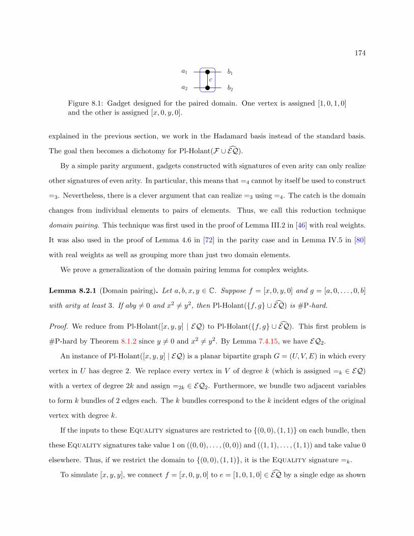
174

a1

a2

b1

b2

c

Figure 8.1: Gadget designed for the paired domain. One vertex is assigned [1, 0, 1, 0]and the other is assigned [x, 0, y, 0].

explained in the previous section, we work in the Hadamard basis instead of the standard basis.

The goal then becomes a dichotomy for Pl-Holant(F ∪ EQ).

By a simple parity argument, gadgets constructed with signatures of even arity can only realize

other signatures of even arity. In particular, this means that =4 cannot by itself be used to construct

=3. Nevertheless, there is a clever argument that can realize =3 using =4. The catch is the domain

changes from individual elements to pairs of elements. Thus, we call this reduction technique

domain pairing. This technique was first used in the proof of Lemma III.2 in [46] with real weights.

It was also used in the proof of Lemma 4.6 in [72] in the parity case and in Lemma IV.5 in [80]

with real weights as well as grouping more than just two domain elements.

We prove a generalization of the domain pairing lemma for complex weights.

Lemma 8.2.1 (Domain pairing). Let a, b, x, y ∈ C. Suppose f = [x, 0, y, 0] and g = [a, 0, . . . , 0, b]

with arity at least 3. If aby 6= 0 and x2 6= y2, then Pl-Holant(f, g ∪ EQ) is #P-hard.

Proof. We reduce from Pl-Holant([x, y, y] | EQ) to Pl-Holant(f, g ∪ EQ). This first problem is

#P-hard by Theorem 8.1.2 since y 6= 0 and x2 6= y2. By Lemma 7.4.15, we have EQ2.

An instance of Pl-Holant([x, y, y] | EQ) is a planar bipartite graph G = (U, V,E) in which every

vertex in U has degree 2. We replace every vertex in V of degree k (which is assigned =k ∈ EQ)

with a vertex of degree 2k and assign =2k ∈ EQ2. Furthermore, we bundle two adjacent variables

to form k bundles of 2 edges each. The k bundles correspond to the k incident edges of the original

vertex with degree k.

If the inputs to these Equality signatures are restricted to (0, 0), (1, 1) on each bundle, then

these Equality signatures take value 1 on ((0, 0), . . . , (0, 0)) and ((1, 1), . . . , (1, 1)) and take value 0

elsewhere. Thus, if we restrict the domain to (0, 0), (1, 1), it is the Equality signature =k.

To simulate [x, y, y], we connect f = [x, 0, y, 0] to e = [1, 0, 1, 0] ∈ EQ by a single edge as shown

175

in Figure 8.1 to form a gadget with signature

h(a1, a2, b1, b2) =∑c=0,1

f(a1, b1, c) · e(a2, b2, c).

We replace every (degree 2) vertex in U (which is assigned [x, y, y]) by a degree 4 vertex assigned

h, where the variables of h are bundled as (a1, a2) and (b1, b2).

The vertices in this new graph G′ are connected as in the original graph G, except that every

original edge is replaced by two edges that connect to the same side of the gadget in Figure 8.1.

Notice that h is only connected by (a1, a2) and (b1, b2) to some bundle of two incident edges of

an Equality signature. Since this Equality signature enforces that the value on each bundle is

either (0, 0) or (1, 1), we only need to consider the restriction of h to the domain (0, 0), (1, 1). On

this domain, h = [x, y, y] is a symmetric signature of arity 2. Therefore, the Holant of G′ has the

same Holant value as the original graph G.

There are two scenarios that lead to Lemma 8.2.1. The proof of the first is immediate.

Corollary 8.2.2. Let a, b, x, y ∈ C. Suppose f = [x, 0, y] and g = [a, 0, . . . , 0, b] with arity at

least 3. If abxy 6= 0 and x4 6= y4, then Pl-Holant(f, g ∪ EQ) is #P-hard.

Proof. Connect three copies of f = [x, 0, y] to [1, 0, 1, 0], with one on each edge, to get x[x2, 0, y2, 0]

and apply Lemma 8.2.1.

The second scenario that leads to Lemma 8.2.1 is Lemma 8.2.4. The proof of Lemma 8.2.4

applies Corollary 8.2.2 after interpolating a unary signature in one of two ways. The next lemma

considers one of those ways.

Lemma 8.2.3. Let x ∈ C. Suppose F is a set of signatures containing f = [1, x, 1]. If x 6∈ 0,±1

and Mf has infinite order modulo a scalar, then

Pl-Holant(F ∪ [a, b] ∪ EQ) ≤T Pl-Holant(F ∪ EQ)

for any a, b ∈ C.

176

Proof. Consider the unary recursive construction (Mf , s) in Figure 6.1, where s = [ 10 ]. The deter-

minant of Mf is 1− x2 6= 0. The determinant of [s Mfs] is x 6= 0. By assumption, Mf has infinite

order modulo a scalar. Therefore, we can interpolate any unary signature by Lemma 6.2.4.

Lemma 8.2.4. Let a, b ∈ C. Suppose f = [a, 0, . . . , 0, b] with arity at least 3. If ab 6= 0 and a4 6= b4,

then Pl-Holant(f ∪ EQ) is #P-hard.

Proof. Since a 6= 0, we normalize f to [1, 0, . . . , 0, x], where x 6= 0 and x4 6= 1. If the arity of f

is even, then after some number of self-loops, we have [1, 0, x] and are done by Corollary 8.2.2.

Otherwise, the arity of f is odd. After some number of self-loops, we have g = [1, 0, 0, x]. If we had

the signature [1, 1], then we could connect this to g to get [1, 0, x] and be done by Corollary 8.2.2.

We now show how to interpolate [1, 1] in one of two ways. In either case, we use the signature

[1, x], which we obtain via a self-loop on g.

Suppose <(x), the real part of x, is nonzero. Connecting [1, x] to [1, 0, 1, 0] gives h = [1, x, 1].

The eigenvalues of Mh are λ± = 1± x. Since <(x) 6= 0 iff |λ+λ− | 6= 1, the ratio of the eigenvalues is

not a root of unity, so Mh has infinite order modulo a scalar. Therefore, we can interpolate [1, 1]

by Lemma 8.2.3.

Otherwise, <(x) = 0 but x is not a root of unity since x 6= ±i. Connecting [1, x] to g gives

h = [1, 0, x2]. Consider the unary recursive construction (Mh, s) in Figure 6.1, where s = [ 1x ]. The

determinant of Mh is x2 6= 0, so its eigenvalues are nonzero. Also, the determinant of [s Mhs] is

x(x2 − 1) 6= 0. The ratio of the eigenvalues of Mh is x2, which is not a root of unity since x is not

a root of unity. Therefore Mh has infinite order modulo a scalar and we can interpolate [1, 1] by

Lemma 6.2.4.

8.3 Mixing of Tractable Signatures

In this section, we determine which tractable signatures combine to give #P-hardness. To help

understand the various cases considered in the lemmas, Figure 8.2 contains a Venn diagram of the

signatures in A , P, and M .

The first two lemmas consider the case when one of the signatures is unary.

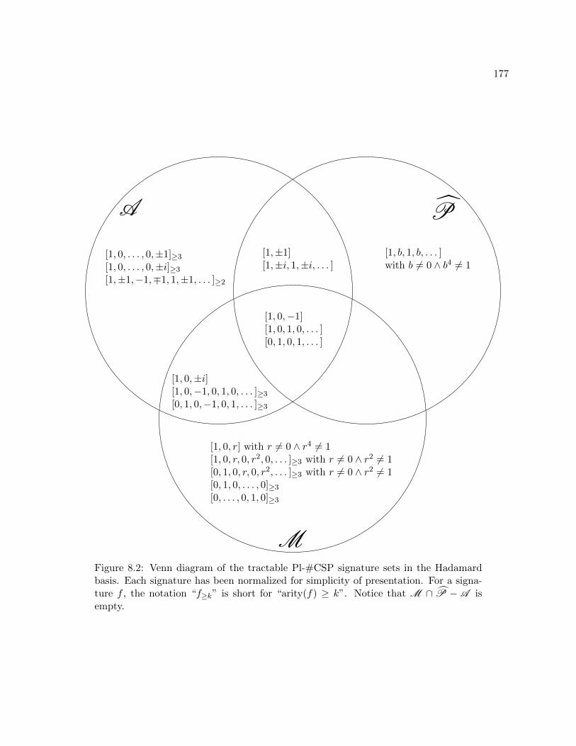
177

A P

M

[1, 0,−1][1, 0, 1, 0, . . . ][0, 1, 0, 1, . . . ]

[1,±1][1,±i, 1,±i, . . . ]

[1, 0,±i][1, 0,−1, 0, 1, 0, . . . ]≥3

[0, 1, 0,−1, 0, 1, . . . ]≥3

[1, 0, . . . , 0,±1]≥3

[1, 0, . . . , 0,±i]≥3

[1,±1,−1,∓1, 1,±1, . . . ]≥2

[1, b, 1, b, . . . ]with b 6= 0 ∧ b4 6= 1

[1, 0, r] with r 6= 0 ∧ r4 6= 1[1, 0, r, 0, r2, 0, . . . ]≥3 with r 6= 0 ∧ r2 6= 1[0, 1, 0, r, 0, r2, . . . ]≥3 with r 6= 0 ∧ r2 6= 1[0, 1, 0, . . . , 0]≥3

[0, . . . , 0, 1, 0]≥3

Figure 8.2: Venn diagram of the tractable Pl-#CSP signature sets in the Hadamardbasis. Each signature has been normalized for simplicity of presentation. For a signa-ture f , the notation “f≥k” is short for “arity(f) ≥ k”. Notice that M ∩ P − A isempty.

178

Lemma 8.3.1. Let a, b ∈ C. Suppose f ∈ A − P. If ab 6= 0 and a4 6= b4, then the problem

Pl-Holant([a, b], f ∪ EQ) is #P-hard.

Proof. Up to a nonzero scalar, the possibilities for f are

• [1, 0,±i];

• [1, 0, . . . , 0, x] of arity at least 3 with x4 = 1;

• [1,±1,−1,∓1, 1,±1,−1,∓1, . . . ] of arity at least 2;

• [1, 0,−1, 0, 1, 0,−1, 0, . . . , 0 or 1 or (−1)] of arity at least 3;

• [0, 1, 0,−1, 0, 1, 0,−1, . . . , 0 or 1 or (−1)] of arity at least 3.

We handle these cases below.

1. Suppose f = [1, 0,±i]. Connecting [a, b] to [1, 0, 1, 0] gives [a, b, a], and connecting two copies

of [1, 0,±i] to [a, b, a], one on each edge, gives g = [a,±ib,−a]. Then Pl-Holant(g | EQ) is

#P-hard by Theorem 8.1.2.

2. Suppose f = [1, 0, . . . , 0, x] of arity at least 3 with x4 = 1. Connecting [a, b] to f gives

g = [a, 0, . . . , 0, bx] of arity at least 2. Note that (bx)4 = b4 6= a4. If the arity of g is exactly 2,

then Pl-Holant(f, g ∪ EQ) is #P-hard by Corollary 8.2.2, so we are done. Otherwise, the

arity of g is at least 3 and Pl-Holant(g ∪ EQ) is #P-hard by Lemma 8.2.4.

3. Suppose f = [1,±1,−1, . . . ] of arity at least 2. Connecting some number of [1, 0] gives

[1,±1,−1] of arity exactly 2. Connecting [a, b] to [1, 0, 1, 0] gives [a, b, a] and connecting two

copies of [a, b, a] to [1,±1,−1], one on each edge, gives g = [a2 ± 2ab− b2,±(a2 + b2),−a2 ±

2ab+ b2]. This is easily verified by

a b

b a

1 ±1

±1 −1

a b

b a

=

a2 ± 2ab− b2 ±(a2 + b2)

±(a2 + b2) −a2 ± 2ab+ b2

.Then Pl-Holant(g | EQ) is #P-hard by Theorem 8.1.2.

4. Suppose f = [1, 0,−1, 0, . . . ] of arity at least 3. Connecting some number of [1, 0] gives g =

[1, 0,−1, 0] of arity exactly 3. Connecting [a, b] to g gives h = [a,−b,−a]. Then Pl-Holant(h |

EQ) is #P-hard by Theorem 8.1.2.

179

5. The argument for f = [0, 1, 0,−1, . . . ] is similar to the previous case.

Lemma 8.3.2. Let a, b ∈ C. If f ∈ M − A and ab 6= 0, then Pl-Holant([a, b], f ∪ EQ) is

#P-hard.

Proof. Up to a nonzero scalar, the possibilities for f are as follows:

• [1, 0, r] with r 6= 0 and r4 6= 1;

• [1, 0, r, 0, r2, 0, . . . ] of arity at least 3 with r 6= 0 and r2 6= 1;

• [0, 1, 0, r, 0, r2, . . . ] of arity at least 3 with r 6= 0 and r2 6= 1;

• [0, 1, 0, . . . , 0] of arity at least 3;

• [0, . . . , 0, 1, 0] of arity at least 3.

We handle these cases below.

1. Suppose f = [1, 0, r] with r4 6= 1 and r 6= 0. Connecting [a, b] to [1, 0, 1, 0] gives [a, b, a] and

connecting two copies of [1, 0, r] to [a, b, a], one on each edge, gives g = [a, br, ar2]. If a2 6= b2,

then Pl-Holant(g | EQ) is #P-hard by Theorem 8.1.2.

Otherwise, a2 = b2 and we begin by connecting [a, b] to [1, 0, r] to get [a, br]. Then by the same

construction, we have g = [a, br2, ar2] and Pl-Holant(g | EQ) is #P-hard by Theorem 8.1.2.

2. Suppose f = [1, 0, r, 0, . . . ] of arity at least 3 with r2 6= 1 and r 6= 0. Connecting some number

of [1, 0] gives g = [1, 0, r, 0] of arity exactly 3. Connecting [a, b] to g gives h = [a, br, a]. If

a2 6= b2r, then Pl-Holant(h | EQ) is #P-hard by Theorem 8.1.2.

Otherwise, a2 = b2r and we begin by connecting [1, 0] and [a, b] to [1, 0, r, 0] to get [a, br].

Then by the same construction, we have g = [a, br2, ar] and Pl-Holant(g | EQ) is #P-hard by

Theorem 8.1.2.

3. The argument for f = [0, 1, 0, r, . . . ] is similar to the previous case.

4. Suppose f = [0, 1, 0, . . . , 0] of arity k ≥ 3. Connecting k − 2 copies of [a, b] to f gives

g = ak−3[(k − 2)b, a, 0]. Then Pl-Holant(g | EQ) is #P-hard by Theorem 8.1.2.

5. The argument for f = [0, . . . , 0, 1, 0] is similar to the previous case.

Now we consider the general case of two signatures from two different tractable sets. Three

tractable sets give rise to three pairs of tractable sets to consider, each of which is covered in one

180

of the next three lemmas.

Lemma 8.3.3. If f ∈ A − P and g ∈ P −A , then Pl-Holant(f, g ∪ EQ) is #P-hard.

Proof. The only possibility for g is [a, b, a, b, . . . ], where ab 6= 0 and a4 6= b4. Connecting some

number of [1, 0] to g gives [a, b] and we are done by Lemma 8.3.1.

Lemma 8.3.4. If f ∈ A −M and g ∈M −A , then Pl-Holant(f, g ∪ EQ) is #P-hard.

Proof. Suppose f does not contain a 0 entry. Then after connecting some number of [1, 0] to f , we

have a unary signature [a, b] with ab 6= 0, and are done by Lemma 8.3.2.

Otherwise, f contains a 0 entry. Then f = [x, 0, . . . , 0, y] of arity at least 3 with xy 6= 0 (and

x4 = y4). Up to a nonzero scalar, the possibilities for g are as follows:

• [1, 0, r] with r 6= 0 and r4 6= 1;

• [1, 0, r, 0, r2, 0, . . . ] of arity at least 3 with r 6= 0 and r2 6= 1;

• [0, 1, 0, r, 0, r2, . . . ] of arity at least 3 with r 6= 0 and r2 6= 1;

• [0, 1, 0, 0, . . . , 0] of arity at least 3;

• [0, . . . , 0, 0, 1, 0] of arity at least 3.

We handle these cases below.

1. Suppose g = [1, 0, r] with r 6= 0 and r4 6= 1. Then we are done by Corollary 8.2.2.

2. Suppose g = [1, 0, r, 0, . . . ] of arity at least 3 with r 6= 0 and r2 6= 1. After connecting some

number of [1, 0] to g, we have h = [1, 0, r, 0] of arity exactly 3. Then Pl-Holant(f, h ∪ EQ)

is #P-hard by Lemma 8.2.1.

3. Suppose g = [0, 1, 0, r, . . . ] of arity at least 3 with r 6= 0 and r2 6= 1. After connecting some

number of [1, 0] to g, we have h = [0, 1, 0, r] of arity exactly 3. Connecting two more copies

of [1, 0] to h gives [0, 1]. Then we apply a holographic transformation by T = [ 0 11 0 ], so f is

transformed to f = [y, 0, . . . , 0, x] and h is transformed to h = [r, 0, 1, 0]. Every even arity

signature in EQ remains unchanged after a holographic transformation by T . By attaching

[0, 1]T = [1, 0] to every even arity signature in T EQ, we obtain all of the odd arity signatures

in EQ again. Then Pl-Holant(f , h ∪ EQ) is #P-hard by Lemma 8.2.1.

181

...

Figure 8.3: The vertices are assigned g = [0, 1, 0, . . . , 0].

4. Suppose g = [0, 1, 0, . . . , 0] of arity k ≥ 3. The gadget in Figure 8.3 with g assigned to

both vertices has signature h = [k − 1, 0, 1]. Then Pl-Holant(f, h ∪ EQ) is #P-hard by

Corollary 8.2.2.

5. The argument for g = [0, . . . , 0, 1, 0] is similar to the previous case.

Lemma 8.3.5. If f ∈ M − P and g ∈ P −M and f, g 6⊆ A , Pl-Holant(f, g ∪ EQ) is

#P-hard.

Proof. The only possibility for g is [a, b, a, b, . . . ] with ab 6= 0. Connecting some number of [1, 0] to

g gives h = [a, b]. If f 6∈ A , then Pl-Holant(f, h ∪ EQ) is #P-hard by Lemma 8.3.2. Otherwise,

f ∈ A , so g 6∈ A and Pl-Holant(f, g ∪ EQ) is #P-hard by Lemma 8.3.3.

We summarize this section with the following theorem, which says that the tractable signature

sets cannot mix. Signatures from different tractable sets, when put together, lead to #P-hardness.

Theorem 8.3.6 (No Mixing). Let F be any set of symmetric, complex-valued signatures in Boolean

variables. If F ⊆ A ∪ P ∪M , then Pl-Holant(F ∪ EQ) is #P-hard unless F ⊆ A , F ⊆ P, or

F ⊆M , in which case Pl-Holantc(F ∪ EQ) is tractable.

Proof. If F is a subset of A , P, or M , then the tractability is given in Theorem 8.1.4. Otherwise

F is not a subset of A , P, or M . Then F contains a signature g ∈ (P ∪M )−A since F 6⊆ A .

Suppose F contains a signature f ∈ A −P−M . If g ∈ P−A , then Pl-Holant(F∪EQ) is #P-hard

by Lemma 8.3.3. Otherwise, g ∈M −A and Pl-Holant(F ∪ EQ) is #P-hard by Lemma 8.3.4.

Now assume that F ⊆ P ∪M . Since (P ∩M ) − A is empty (see Figure 8.2), either g ∈

P−M −A or g ∈M −P−A . If g ∈ P−M −A , then there exists a signature f ∈M −P since

F 6⊆ P. In which case, Pl-Holant(F∪EQ) is #P-hard by Lemma 8.3.5. Otherwise, g ∈M−P−A

and there exists a signature f ∈ P−M since F 6⊆M . In which case, Pl-Holant(F∪EQ) is #P-hard

by Lemma 8.3.5.

182

8.4 Pinning for Planar Graphs

The idea of “pinning” is a common reduction technique between counting problems. For the #CSP

framework, pinning fixes some variables to specific values of the domain by means of the constant

functions [17, 58, 13, 80]. In particular, for counting graph homomorphisms, pinning is used when

the input graph is connected and the target graph is disconnected. In this case, pinning a vertex of

the input graph to a vertex of the target graph forces all the vertices of the input graph to map to

the same connected component of the target graph [59, 14, 70, 122, 23]. For the Boolean domain,

the constant 0 and constant 1 functions are the signatures [1, 0] and [0, 1] respectively.

From these works, the most relevant pinning lemma for the Pl-#CSP framework is by Dyer,

Goldberg, and Jerrum in [58], where they show how to pin in the #CSP framework. However, the

proof of this pinning lemma is highly nonplanar. Cai, Lu, and Xia [46] overcame this difficultly in

the proof of their dichotomy theorem for the real-weighted Pl-#CSP framework by first undergoing

a holographic transformation by the Hadamard matrix H =[

1 11 −1

]and then pinning in this

Hadamard basis.3 We stress that this holographic transformation is necessary. Indeed, if one were

able to pin in the standard basis of the Pl-#CSP framework, then P = #P would follow since

Pl-#CSP(M ) is tractable but Pl-#CSP(M ∪ [1, 0], [0, 1]) is #P-hard by our main dichotomy in

Theorem 8.5.3 (or, more specifically, by Lemma 8.3.2).

Since Pl-#CSP(F) is equivalent to Pl-Holant(F ∪ EQ), the expression of Pl-#CSP(F) in the

Hadamard basis is Pl-Holant(HF ∪ EQ). Then we already have [1, 0] ∈ EQ, so pinning in the

Hadamard basis of Pl-#CSP(F) amounts to obtaining the missing signature [0, 1].

8.4.1 The Road to Pinning

We begin the road to pinning with a lemma that assumes the presence of [0, 0, 1] = [0, 1]⊗2, which

is the tensor product of two copies of [0, 1]. In our pursuit to realize [0, 1], this may be as close as we

can get, such as when every signature has even arity. Another roadblock to realizing [0, 1] is when

every signature has even parity. Recall that a signature has even parity if its support is on entries

3The pinning in [46], which is accomplished in Section IV, is not summarized in a single statement but is impliedby the combination of all the results in that section.

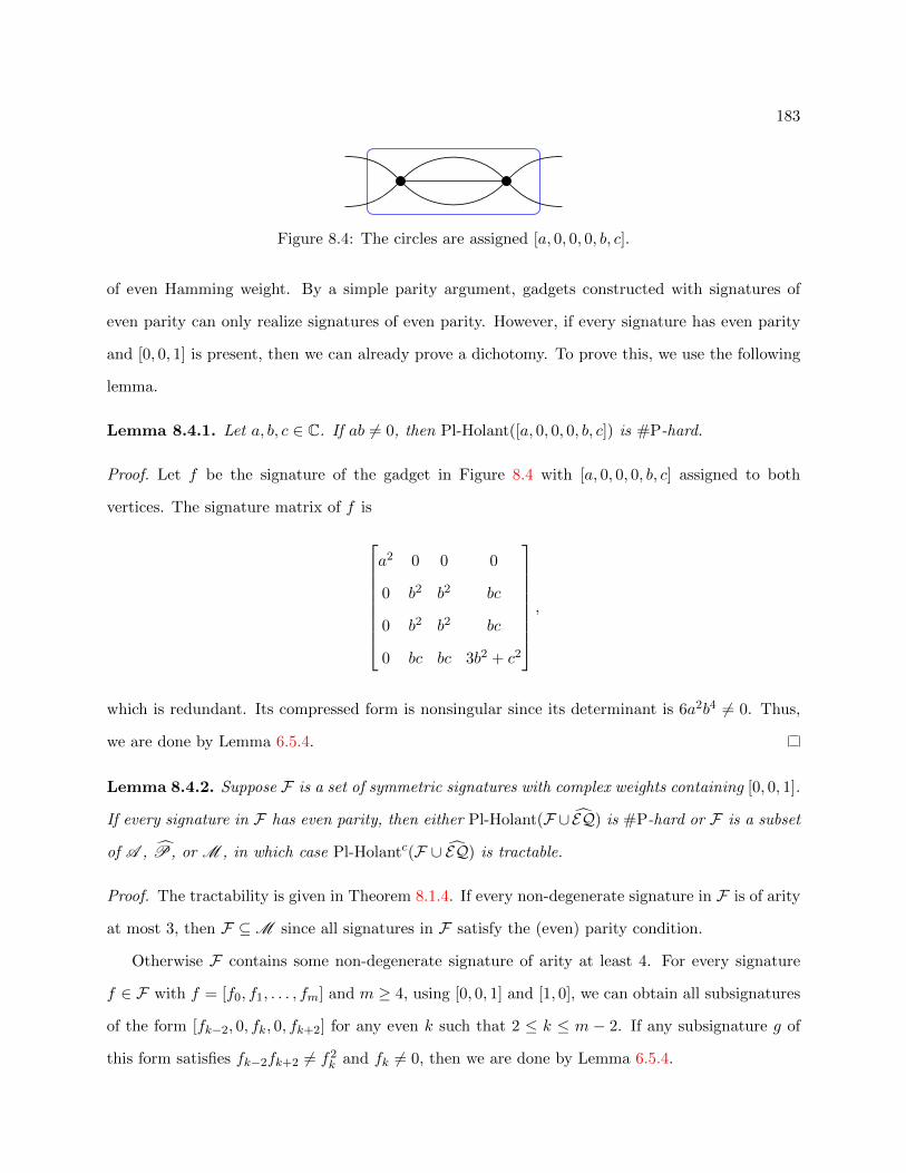
183

Figure 8.4: The circles are assigned [a, 0, 0, 0, b, c].

of even Hamming weight. By a simple parity argument, gadgets constructed with signatures of

even parity can only realize signatures of even parity. However, if every signature has even parity

and [0, 0, 1] is present, then we can already prove a dichotomy. To prove this, we use the following

lemma.

Lemma 8.4.1. Let a, b, c ∈ C. If ab 6= 0, then Pl-Holant([a, 0, 0, 0, b, c]) is #P-hard.

Proof. Let f be the signature of the gadget in Figure 8.4 with [a, 0, 0, 0, b, c] assigned to both

vertices. The signature matrix of f is

a2 0 0 0

0 b2 b2 bc

0 b2 b2 bc

0 bc bc 3b2 + c2

,

which is redundant. Its compressed form is nonsingular since its determinant is 6a2b4 6= 0. Thus,

we are done by Lemma 6.5.4.

Lemma 8.4.2. Suppose F is a set of symmetric signatures with complex weights containing [0, 0, 1].

If every signature in F has even parity, then either Pl-Holant(F ∪EQ) is #P-hard or F is a subset

of A , P, or M , in which case Pl-Holantc(F ∪ EQ) is tractable.

Proof. The tractability is given in Theorem 8.1.4. If every non-degenerate signature in F is of arity

at most 3, then F ⊆M since all signatures in F satisfy the (even) parity condition.

Otherwise F contains some non-degenerate signature of arity at least 4. For every signature

f ∈ F with f = [f0, f1, . . . , fm] and m ≥ 4, using [0, 0, 1] and [1, 0], we can obtain all subsignatures

of the form [fk−2, 0, fk, 0, fk+2] for any even k such that 2 ≤ k ≤ m − 2. If any subsignature g of

this form satisfies fk−2fk+2 6= f2k and fk 6= 0, then we are done by Lemma 6.5.4.

184

Otherwise all subsignatures of signatures in F of the above form satisfy fk−2fk+2 = f2k or

fk = 0. There are two types of signatures with this property. In the first type, the signature entries

of even Hamming weight form a geometric progression. More specifically, the signatures of the first

type have the form

[αn, 0, αn−1β, 0, . . . , 0, αβn−1, 0, βn] or [αn, 0, αn−1β, 0, . . . , 0, αβn−1, 0, βn, 0]

for some α, β ∈ C, which are in M . In the second type, the signatures have arity at least 4 or 5

and are of the form [x, 0, . . . , 0, y] or [x, 0, . . . , 0, y, 0] respectively, with xy 6= 0 and an odd number

of 0’s between x and y (since they have even parity). If all signatures in F are of the first type,

then F ⊆M .

Otherwise F contains a signature f of the second type. Suppose f = [x, 0, . . . , 0, y, 0] of arity at

least 5 with xy 6= 0. After some number of self-loops, we have g = [x, 0, 0, 0, y, 0] of arity exactly 5.

Then we are done by Lemma 8.4.1.

Otherwise f = [x, 0, . . . , 0, y] of arity at least 4 with xy 6= 0. If x4 6= y4, then we are done by

Lemma 8.2.4.

Otherwise x4 = y4. This puts every signature of the second type in A . Therefore F ⊆ A ∪M

and we are done by Theorem 8.3.6.

The conclusion of every result in the rest of this section states that we are able to pin (under

various assumptions on F). Formally speaking, we repeatedly prove that Pl-Holantc(F ∪ EQ) is

#P-hard (or in P) if and only if Pl-Holant(F ∪ EQ) is #P-hard (or in P). The difference between

these two counting problems is the presence of [0, 1] in Pl-Holantc(F ∪ EQ). We always prove this

statement in one of three ways:

1. either we show that Pl-Holantc(F ∪ EQ) is tractable (so Pl-Holant(F ∪ EQ) is as well);

2. or we show that Pl-Holant(F ∪ EQ) is #P-hard (so Pl-Holantc(F ∪ EQ) is as well);

3. or we show how to reduce Pl-Holantc(F ∪ EQ) to Pl-Holant(F ∪ EQ) by realizing [0, 1] using

signatures in F ∪ EQ.

Lemma 8.4.3. Let F be any set of complex-weighted symmetric signatures containing [0, 0, 1].

185

Figure 8.5: The circles are assigned [1, 0, 1, 0] and the triangles are assigned [1, 0, x].

Then Pl-Holantc(F ∪ EQ) is #P-hard (or in P) iff Pl-Holant(F ∪ EQ) is #P-hard (or in P).

Proof. If we had a unary signature [a, b] where b 6= 0, then connecting [a, b] to [0, 0, 1] gives the

signature [0, b], which is [0, 1] after normalizing. Thus, in order to reduce Pl-Holantc(F ∪ EQ) to

Pl-Holant(F ∪EQ) by constructing [0, 1], it suffices to construct a unary signature [a, b] with b 6= 0.

For every signature f ∈ F with f = [f0, f1, . . . , fm], using [0, 0, 1] and [1, 0], we can obtain all

subsignatures of the form [fk−1, fk] for any odd k such that 1 ≤ k ≤ m. If any subsignature satisfies

fk 6= 0, then we can construct [0, 1].

Otherwise all signatures in F have even parity and we are done by Lemma 8.4.2.

There are two scenarios that lead to Lemma 8.4.3, which are the focus of the next two lemmas.

Lemma 8.4.4. For x ∈ C, let F be any set of complex-weighted symmetric signatures containing

[1, 0, x] such that x /∈ 0,±1. Then Pl-Holantc(F∪EQ) is #P-hard (or in P) iff Pl-Holant(F∪EQ)

is #P-hard (or in P).

Proof. There are two cases. In either case, we realize [0, 0, 1] and finish by applying Lemma 8.4.3.

First we claim that the conclusion holds provided |x| /∈ 0, 1. Combining k copies of [1, 0, x]

gives [1, 0, xk]. Since |x| /∈ 0, 1, x is neither zero nor a root of unity, so we can use polynomial

interpolation to realize [a, 0, b] for any a, b ∈ C, including [0, 0, 1].

Otherwise |x| = 1. The gadget in Figure 8.5 has signature [f0, f1, f2] = [1+x2, 0, 2x]. If x = ±i,

then we have [0, 0,±2i], which is [0, 0, 1] after normalizing.

Otherwise x 6= ±i, so f0 6= 0. Since x 6= 0, we have f2 6= 0. Since x 6= ±1, we have |f0| < 2.

However, |f2| = 2. Therefore, after normalizing, the signature [1, 0, y] with y = 2x1+x2

has |y| > 1,

so it can interpolate [0, 0, 1] by our initial claim since |y| /∈ 0, 1.

186

Lemma 8.4.5. Let F be any set of complex-weighted symmetric signatures containing a signature

[f0, f1, . . . , fn] that is not identically zero but has f0 = 0. Then Pl-Holantc(F ∪ EQ) is #P-hard (or

in P) iff Pl-Holant(F ∪ EQ) is #P-hard (or in P).

Proof. If f1 6= 0, then we connect n − 1 copies of [1, 0] to f to get [0, f1], which is [0, 1] after

normalizing. If f1 = 0, then n ≥ 2. If f2 6= 0, then we connect n − 2 copies of [1, 0] to f to get

[0, 0, f2], which is [0, 0, 1] after normalizing. Then we are done by Lemma 8.4.3. If f1 = f2 = 0,

then n ≥ 3. After some number of self-loops, we get a signature with exactly one or two initial 0’s,

which is one of the above scenarios.

As a significant step toward pinning for any signature set F , we show how to pin given any

binary signature. Some cases resist pinning and are excluded.

Lemma 8.4.6. Let F be any set of complex-weighted symmetric signatures containing a binary

signature f . Then Pl-Holantc(F ∪ EQ) is #P-hard (or in P) iff Pl-Holant(F ∪ EQ) is #P-hard (or

in P) unless f ∈ [0, 0, 0], [1, 0,−1], [1, r, r2], [1, b, 1], up to a nonzero scalar, for any b, r ∈ C.

Proof. Let f = [f0, f1, f2]. If f0 = 0 and either f1 6= 0 or f2 6= 0, then we are done by Lemma 8.4.5.

Otherwise, f = [0, 0, 0] or f0 6= 0, in which case we normalize f0 to 1. If Pl-Holant(f | EQ) is

#P-hard by Theorem 8.1.2, then Pl-Holant(F ∪ EQ) is also #P-hard. Otherwise, f is one of the

tractable cases, which implies that

f ∈ [0, 0, 0], [1, r, r2], [1, 0, x], [1,±1,−1], [1, b, 1].

If f = [1,±1,−1], then we connect f to [1, 0, 1, 0] to get [0,±2], which is [0, 1] after normalizing.

If f = [1, 0, x], then we are done by Lemma 8.4.4 unless x ∈ 0,±1. The remaining cases are all

excluded by assumption, so we are done.

8.4.2 Pinning in the Hadamard Basis

Before we show how to pin in the Hadamard basis, we handle two simple cases.

187

Lemma 8.4.7. If F is a set of signatures containing [1,±i], then we have Pl-Holantc(F ∪ EQ) ≤T

Pl-Holant(F ∪ EQ).

Proof. Connect two copies of [1,±i] to [1, 0, 1, 0] to get [0,±2i], which is [0, 1] after normalizing.

The next lemma considers the signature [1, b, 1, b−1], which we also encounter in Theorem 8.5.1,

the single signature dichotomy.

Lemma 8.4.8. Let b ∈ C. If b /∈ 0,±1, then Pl-Holant([1, b, 1, b−1] ∪ EQ) is #P-hard.

Proof. Connect two copies of [1, 0] to f = [1, b, 1, b−1] to get [1, b]. Connecting this back to f gives

g = [1 + b2, 2b, 2]. Then Pl-Holant(g | EQ) is #P-hard by Theorem 8.1.2.

Now we are ready to prove our pinning result.

Theorem 8.4.9 (Pinning). Let F be any set of complex-weighted symmetric signatures. Then

Pl-Holantc(F ∪ EQ) is #P-hard (or in P) iff Pl-Holant(F ∪ EQ) is #P-hard (or in P).

This theorem does not exclude the possibility that either framework can express a problem of in-

termediate complexity. It merely says that if one framework cannot express a problem of intermedi-

ate complexity, then neither can the other. Our goal is to prove a dichotomy for Pl-Holant(F∪EQ).

By Theorem 8.4.9, this is equivalent to proving a dichotomy for Pl-Holantc(F ∪ EQ).

Proof of Theorem 8.4.9. For simplicity, we normalize the first nonzero entry of every signature in

F to 1. If F contains the degenerate signature [0, 1]⊗n for some n ≥ 1, then we take self-loops on

this signature until we have either [0, 1] or [0, 0, 1] (depending on the parity of n). If we have [0, 1],

we are done. Otherwise, we have [0, 0, 1] and are done by Lemma 8.4.3.

Now assume that any degenerate signature in F is not of the form [0, 1]⊗n. Then we can replace

these degenerate signatures in F by their unary versions using [1, 0]. This does not change the

complexity of the problem. If F contains only unary signatures, then F ⊆ P and Pl-Holantc(F ∪

EQ) is tractable by Theorem 8.1.4.

Otherwise F contains a signature f of arity at least two. We connect some number of [1, 0] to

f until we obtain a signature with arity exactly two. We call the resulting signature the binary

188

prefix of f . If this binary prefix is not one of the exceptional forms in Lemma 8.4.6, then we are

done, so assume that it is one of the exceptional forms.

Now we perform case analysis according to the exceptional forms in Lemma 8.4.6. There are

five cases below because we consider [1, r, r2] as [1, 0, 0] and [1, r, r2] with r 6= 0 as separate cases.

In each case, we either show that the conclusion of the theorem holds or that f ∈ A ∪ P ∪M .

After the case analysis, we then handle all of these tractable f together.

1. Suppose the binary prefix of f is [0, 0, 0]. If f is not identically zero, then we are done by

Lemma 8.4.5.

Thus, in this case, we may assume f = [0, 0, . . . , 0] is identically zero.

2. Suppose the binary prefix of f is [1, 0,−1]. If f is not of the form

[1, 0,−1, 0, 1, 0,−1, 0, . . . , 0 or 1 or (−1)], (8.4.1)

then after one self-loop, we have a signature of arity at least one with 0 as its first entry but

is not identically zero, so we are done by Lemma 8.4.5.

Thus, in this case, we may assume f has the form given in (8.4.1).

3. Suppose the binary prefix of f is [1, 0, 0]. If f is not of the form [1, 0, . . . , 0], then after

connecting some number of [1, 0], we have [1, 0, . . . , 0, x] of arity at least 3, where x 6= 0. If

x4 6= 1, then Pl-Holant(f ∪ EQ) is #P-hard by Lemma 8.2.4, so Pl-Holant(F ∪ EQ) is also

#P-hard.

Otherwise, x4 = 1. Suppose that x is not the last entry in f . Then connecting one fewer

[1, 0] than before, we have g = [1, 0, . . . , 0, x, y] and there are two cases to consider. If the

index of x in g is odd, then after some number of self-loops, we have h = [1, 0, 0, x, y]. The

determinant of the compressed signature matrix of h is −2x2 6= 0. Thus, Holant(h) is #P-hard

by Lemma 6.5.4, so Pl-Holant(F ∪ EQ) is also #P-hard.

Otherwise, the index of x in g is even. After some number of self-loops, we have h =

[1, 0, 0, 0, x, y]. Then by Lemma 8.4.1, Holant(h) is #P-hard, so Pl-Holant(F ∪ EQ) is also

#P-hard.

189

Thus, in this case, we may assume either f = [1, 0, . . . , 0] or f = [1, 0, . . . , 0, x] with x4 = 1.

4. Suppose the binary prefix of f is [1, r, r2], where r 6= 0. If f is not of the form [1, r, . . . , rn],

then after connecting some number of [1, 0], we have [1, r, . . . , rm, y], where y 6= rm+1 and

m ≥ 2. Using [1, 0], we can get [1, r]. If r = ±i, then we are done by Lemma 8.4.7, so assume

that r 6= ±i. Then we can attach [1, r] back to the initial signature some number of times

to get g = [1, r, r2, x] after normalizing, where x 6= r3. We connect [1, r] once more to get

h = [1+r2, r(1+r2), r2 +rx]. If h does not have one of the exceptional forms in Lemma 8.4.6,

then we are done, so assume that it does.

Since the second entry of h is not 0 and x 6= r3, the only possibility is that h has the form

[1, b, 1] up to a scalar. This gives x = r−1. Note that r 6= ±1 since x 6= r3. A self-loop on

g = [1, r, r2, r−1] gives [1 + r2, r + r−1], which is [1, r−1] after normalizing. Connecting this

back to g gives h = [2, 2r, r2 + r−2]. We assume that h has one of the exceptional forms in

Lemma 8.4.6 since we are done otherwise. If h has the form [1, r, r2] up to a scalar, then

r4 = 1, a contradiction, so it must have the form [1, b, 1] up to a scalar. But then r2 = 1,

which is also a contradiction.

Thus, in this case, we may assume f = [1, r, . . . , rn].

5. Suppose the binary prefix of f is [1, b, 1]. If b = ±1, then this binary prefix is degenerate

and was considered in the previous case, so assume that b 6= ±1. If f is not of the form

[1, b, 1, b, . . . ], then suppose that the index of the first entry in f to break the pattern is even.

Then after connecting some number of [1, 0], we have [1, b, 1, . . . , b, y], where y 6= 1. Then

after some number of self-loops and normalizing, we have g = [1, b, 1, b, x], where x 6= 1. The

determinant of its compressed signature matrix is (b2 − 1)(1 − x) 6= 0. Thus, Holant(g) is

#P-hard by Lemma 6.5.4, so Pl-Holant(F ∪ EQ) is also #P-hard.

Otherwise, the index of the first entry in f to break the pattern is odd. Then after connecting

some number of [1, 0], we have [1, b, 1, . . . , 1, y], where y 6= b. Then after some number of self-

loops and normalizing, we have [1, b, 1, x], where x 6= b. We do a self-loop to get g = [2, b+x].

If b = 0, then connecting g to [1, 0, 1, x] gives h = [2, x, 2 + x2]. We assume that h has one

of the exceptional forms in Lemma 8.4.6 since we are done otherwise. Because x 6= 0, the

190

only possibility is that h has the form [1, r, r2] up to a scalar. Then we get x2 = −4, so

g = [2, x] = 2[1,±i] and we are done by Lemma 8.4.7. We use the signature g again below.

Otherwise, b 6= 0. Using [1, 0], we can get h = [1, b, 1]. If the signature matrix Mh of

h has finite order modulo a scalar, then M `h = βI2 for some positive integer ` and some

nonzero complex value β. Thus after normalizing, we can construct the anti-gadget [1,−b, 1]

by connecting ` − 1 copies of h together. Connecting [1, 0] to [1,−b, 1] gives [1,−b] and

connecting this to [1, b, 1, x] gives [1 − b2, 0, 1 − bx]. If 1−bx1−b2 /∈ 0,±1, then we are done by

Lemma 8.4.4.

Otherwise, y = 1−bx1−b2 ∈ 0,±1. For y = 0, we get x = b−1 and are done by Lemma 8.4.8 since

b /∈ 0,±1. For y = 1, we get b = x, a contradiction. For y = −1, we get 2 − b2 − bx = 0.

Then connecting [1,−b, 1] to g = [2, b+ x] gives [2− b2 − bx, x− b] = [0, x− b], which is [0, 1]

after normalizing.

Otherwise, Mh has infinite order modulo a scalar, so we can interpolate [0, 1] by Lemma 8.2.3

since b /∈ 0,±1.

Thus, in this case, we may assume f = [1, b, 1, b, . . . ].

At this point, every signature in F (including the unary signatures) must be of one of the

following forms:

• [0, . . . , 0], which is in A ∩ P ∩M ;

• [1, 0,−1, 0, 1, 0,−1, 0, . . . , 0 or 1 or (−1)], which is in A ∩M ;

• [1, 0, . . . , 0, x], where x4 = 1, which is in A ;

• [1, b, 1, b, . . . , 1 or b], which is in P.

In particular, every possible unary signature either fits into the first case or the last case. Therefore

F ⊆ A ∪ P ∪M and we are done by Theorem 8.3.6.

8.5 Main Result

In this section, we prove our main dichotomy theorem. But first a dichotomy for a single signature.

Theorem 8.5.1. If f is a non-degenerate symmetric signature of arity at least 2 with complex

191

weights in Boolean variables, then Pl-Holant(f ∪ EQ) is #P-hard unless f ∈ A ∪ P ∪M , in

which case the problem is computable in polynomial time.

Proof. When f ∈ A ∪P∪M , the problem is tractable by Theorem 8.1.4. When f 6∈ A ∪P∪M , we

prove that Pl-Holantc(f∪EQ) is #P-hard, which is sufficient because of pinning (Theorem 8.4.9).

Using [1, 0] and [0, 1], we can obtain any subsignature of f .

Notice that once we have [0, 1] and EQ, we can realize every signature in T EQ, where T =

[ 0 11 0 ]. In fact, every even arity signature in EQ is also in T EQ, and we obtain all the odd arity

signatures in T EQ by attaching [0, 1] to all the even arity signatures in EQ. Therefore, a holographic

transformation by T does not change the complexity of the problem. Furthermore, A ∪ P ∪M is

closed under T . We use these facts later.

The possibilities for f can be divided into three cases:

• f satisfies the parity condition;

• f does not satisfy the parity condition but does contain a 0 entry;

• f does not contain a 0 entry.

We handle these cases below.

1. Suppose that f satisfies the parity condition. If f has even parity, then we are done by

Lemma 8.4.2.

Otherwise, f has odd parity. If f has odd arity, then under a holographic transformation by

T = [ 0 11 0 ], f is transformed to f , which has even parity. Then either Pl-Holantc(f ∪ EQ) is

#P-hard by Lemma 8.4.2 (and thus Pl-Holantc(f∪EQ) is also #P-hard), or f ∈ A ∪P∪M

(and thus f ∈ A ∪ P ∪M ).

Otherwise, the arity of f is even. Connect [0, 1] to f to get a signature g with even parity

and odd arity. Then either Pl-Holantc(g ∪ EQ) is #P-hard by Lemma 8.4.2 (and thus

Pl-Holantc(f ∪ EQ) is also #P-hard), or g ∈ A ∪ P ∪M . In the latter case, it must

be that g ∈ M since non-degenerate generalized equality signatures cannot have both even

parity and odd arity. (See Figure 8.2 at the end of the Appendix, which contains a Venn

diagram of the signatures in A ∪ P ∪M , up to constant factors.) In particular, the even

parity entries of g form a geometric progression. Therefore f ∈ M since f has odd parity

192

and the same geometric progression among its odd parity entries.

2. Suppose that f contains a 0 entry but does not satisfy the parity condition. Since f does not

satisfy the parity condition, there must be at least two nonzero entries separated by an even

number of 0 entries. Thus, f contains a subsignature g = [a, 0, . . . , 0, b] of arity n = 2k+1 ≥ 1,

where ab 6= 0.

If k = 0, then n = 1 and we can shift either to the right or to the left and find the 0 entry

in f and obtain a binary subsignature h of the form [c, d, 0] or [0, c, d], where cd 6= 0. Then

Pl-Holant(h | EQ) is #P-hard by Theorem 8.1.2, so Pl-Holant(f ∪ EQ) is also #P-hard.

Otherwise k ≥ 1, so n ≥ 3. If a4 6= b4, then Pl-Holant(g∪ EQ) is #P-hard by Lemma 8.2.4,

so Pl-Holant(f ∪ EQ) is also #P-hard.

Otherwise, a4 = b4, so g ∈ A . If f = g, then we are done, so assume that f 6= g, which

implies that there is another entry just before a or just after b. If this entry is nonzero, then

f has a subsignature h of the form [c, a, 0] or [0, b, d], where cd 6= 0. Then Pl-Holant(h | EQ)

is #P-hard by Theorem 8.1.2, so Pl-Holant(f ∪ EQ) is also #P-hard.

Otherwise, this entry is 0 and f has a subsignature h of the form

[0, a, 0, . . . , 0, b] or [a, 0, . . . , 0, b, 0]

of arity at least 4. If the arity of h is even, then after some number of self-loops, we have a

signature h′ of the form [0, a, 0, 0, b] or [a, 0, 0, b, 0] of arity exactly 4. Then Pl-Holant(h′) is

#P-hard by Lemma 6.5.4 since ab 6= 0, so Pl-Holant(f ∪ EQ) is also #P-hard.

Otherwise, the arity of h is odd. After some number of self-loops, we have a signature h′ of

the form [0, a, 0, 0, 0, b] or [a, 0, 0, 0, b, 0] of arity exactly 5. Then Pl-Holant(h′) is #P-hard by

Lemma 8.4.1 since ab 6= 0, so Pl-Holant(f ∪ EQ) is also #P-hard.

3. Suppose f contains no 0 entry. If f has a binary subsignature g such that Pl-Holant(g | EQ)

is #P-hard by Theorem 8.1.2, then Pl-Holant(f ∪ EQ) is also #P-hard.

Otherwise every binary subsignature [a, b, c] of f satisfies the conditions of some tractable case

in Theorem 8.1.2. The three possible tractable cases are degenerate with condition ac = b2

(case 1), affine A with condition ac = −b2 ∧ a = −c (case 3), and a Hadamard-transformed

193

product type P with condition a = c (case 4). If every binary subsignature [a, b, c] of f

satisfies ac = b2, then f is degenerate, a contradiction. If every binary subsignature [a, b, c]

of f satisfies ac = −b2 ∧ a = −c, then f = [1,±1,−1,∓1, 1,±1,−1,∓1, . . . ] ∈ A (up to a

scalar) and we are done. If every binary subsignature [a, b, c] of f satisfies a = c, then f ∈ P

and we are done.

Otherwise, there exists two binary subsignatures of f that do not satisfy the same tractable

case in Theorem 8.1.2. More specifically, f has arity at least 3 and there exists a ternary

subsignature g = [a, b, c, d] such that h = [a, b, c] and h′ = [b, c, d] exclusively satisfy the

conditions of different tractable cases in Theorem 8.1.2. By symmetry in the statement of the

tractable conditions in Theorem 8.1.2, under a holographic transformation by [ 0 11 0 ], we can

we can switch the order of h and h′. Suppose f contains a binary subsignature that satisfies

the condition of the affine case. Let h be that subsignature. Then for either case of h′, we

have g = [1, ε,−1, ε] after normalizing, where ε2 = 1. Connecting two copies of [0, 1] to g

gives [−1, ε]. Connecting this back to g gives g′ = [0,−2ε, 2]. Then Pl-Holant(g′ | EQ) is

#P-hard by Theorem 8.1.2, so Pl-Holant(f ∪ EQ) is also #P-hard.

Otherwise, we may assume that h satisfies the product-type condition (but not the degenerate

condition) and h′ satisfies the degenerate condition. Then g = [1, b, 1, b−1] after normalizing,

where b2 6= 1. Then Pl-Holant(g | EQ) is #P-hard by Lemma 8.4.8, so Pl-Holant(f ∪ EQ)

is also #P-hard.

Now we are ready to prove our main dichotomy theorem.

Theorem 8.5.2. Let F be any set of symmetric, complex-valued signatures in Boolean variables.

Then Pl-Holant(F∪EQ) is #P-hard unless F ⊆ A , F ⊆ P, or F ⊆M , in which case the problem

is computable in polynomial time.

Proof. The tractability is given in Theorem 8.1.4. When F is not a subset of A , P, or M , we

prove that Pl-Holantc(F ∪ EQ) is #P-hard, which is sufficient because of pinning (Theorem 8.4.9).

For any degenerate signature f ∈ F , we connect some number of [1, 0] to f to get its correspond-

ing unary signature. We replace f by this unary signature, which does not change the complexity.

194

Thus, assume that the only degenerate signatures in F are unary signatures.

If F 6⊆ A ∪P∪M , then the problem is #P-hard by Theorem 8.5.1. Otherwise, F ⊆ A ∪P∪M

and we are done by Theorem 8.3.6.

We also have the corresponding theorem for the Pl-#CSP framework in the standard basis.

Theorem 8.5.3. Let F be any set of symmetric, complex-valued signatures in Boolean variables.

Then Pl-#CSP(F) is #P-hard unless F ⊆ A , F ⊆ P, or F ⊆ M , in which case the problem is

computable in polynomial time.

8.6 Closing Thoughts

Designing the proof One of the anonymous reviewers of [74] made the following comment.

“It is hard to imagine how hard it is to design the case-by-case proof in [Sections 8.2, 8.3,

and 8.4].”

Let me try to explain how this is done. The short answer is that you don’t design the case-by-case

proof. You design the overall structure of the proof and the case-by-case aspects of the proof design

themselves.

One should begin by considering important ideas from previous work that were successful. We

had just finished [29], the Holant dichotomy that was proven in Chapter 7. The hardness proof of

the dichotomy for any set of signatures (see the end of Section 7.5) was easy to prove given the

tools to which we availed ourselves by that point. The primary tool was a dichotomy for a single

signature (Theorem 7.5.1). Thus, the plan is to prove a single signature dichotomy for Pl-#CSP,

which we eventually did in Theorem 8.5.1.

Nearly all of the previous dichotomy theorems for #CSP (including nearly all of the dichotomy

theorems for the special case of counting graph homomorphisms), used the pinning technique. This

makes it an easy decision to attempt to pin in our new setting. As previously discussed, the only

chance of pinning in Pl-#CSP must occur in the Hadamard basis. Thus, the plan is to pin in

Pl-Holant(F ∪ EQ).

195

The other tool used in the Holant dichotomy is “mixing” results, though it is not as clearly

delineated as in the current chapter (the whole of Section 8.3). Partial mixing with vanishing sig-

natures was given in Section 7.3. The mixing results for signatures in A or P are implicit in the

Pl-#CSPd dichotomy, which was applied in each of the three dichotomies in Subsection 7.4.2. Any-

way, after applying a single signature dichotomy, what you are left with is a bunch of individually

tractable signatures. Thus, it is natural to prove some mixing results.

Furthermore, it is a good idea to prove this mixing result as soon as possible. The proofs of

these dichotomy theorems are typically begun with a (possibly rough) conjecture of the tractable

cases. By proving mixing results, you gain a clearer picture of the final dichotomy that you are

trying to prove. For example, when we began [29], we knew that a new tractable case would involve

vanishing signatures. But even after characterizing them (presented here in Section 4.4), we still

didn’t know the statement of the dichotomy that we wanted to prove. We had to determine what

signatures combine with vanishing ones and remain tractable. This is where (attempting to) prove

a dichotomy theorem helps you. You just try to prove as much hardness as possible. When you

can prove no more, you stop and try to show instead that the problem is tractable.

Now the question to ask is: how can the mixing results be proved? This is generally done by

reduction from small arity cases, which is (partially) why we first proved a planar Holant dichotomy

for a single signature of arity 4 (presented here in Chapter 6). It also happened that we used the

technique of domain pairing. This technique was also used to prove the Pl-#CSP dichotomy with

real weights, so it was natural to see how this technique could help us as well.

Given this plan for the high-level proof structure, you then go and execute. The “design” of our

proof at the “case” level (in Sections 8.2, 8.3, and 8.4) is simply a result of optimizing the proof.

Style of presentation I no longer like the

“problem A is #P-hard (or in P) iff problem B is #P-hard (or in P)”

style of presentation. It would not bother me so much if it were just used once in, say, the Pinning

Theorem (Theorem 8.4.9). In total though, it is used five times, and the statements of these results

are rather wordy because of it.

196

I think it is possible to reorganize and restate these results as various cases that can be nicely

tied together in a newly worded pinning lemma. This style of presentation is similar to that in

Chapter 11. Roughly speaking, the style used there can be described as follows. First, cases are

shown to be #P-hard whenever possible. Second, if there is some tractable case, then its tractability

is briefly mentioned in prose between hardness proofs to motivate why that case is excluded in the

next proof of #P-hardness (and often why it is excluded in many future proofs of #P-hardness as

well). Finally, everything is tied together in some capstone theorem that considers each case and

either shows that it is tractable or shows that it is #P-hard.

197

Chapter 9

Interlude to Compute Some Gadget

Signatures over General Domains

This chapter contains no complexity results. It exists so that complexity results can be proved

in the next two chapters, which study the computational complexity of higher domain Holant

problems. With higher domains, it becomes increasing difficult to verify that a particular gadget

has a particular signature. This work was published in [32, 33].

9.1 Discussion

In the next two chapters, some of the more difficult claims to verify are those when we say that a

particular F-gate has a particular signature. This is an essential difficultly that cannot be avoided.

We are proving that Pl-Holantκ(F) is #P-hard for various F (and computing the signature of an

F-gate is a generalization of this problem). Thus, one should not expect to be able to compute

these signatures significantly faster in general than what the naive algorithm can do.

This has always been an issue for any dichotomy theorem about counting problems, but with

larger domain sizes, we seem to be reaching the limit of what can be computed by hand for the

signatures of gadget constructions that are presented in our proofs. To counter this, the standard

techniques are to utilize the smallest gadgets (that suffice) or an infinite family of related gadgets

198

with a (small) description of finite size, which we certainly employ. Additionally, we point out some

tricks, where they exist, to save as much work as possible.

Beyond all this, we also face another problem. We would like to express the signature of a

gadget as a function of the domain size. To compute the signature of a gadget for every domain

size is no longer a finite computation. However, each entry of the gadget’s signature is a polynomial

in the domain size of degree at most the number of internal edges in the gadget. To obtain these

polynomials, one can interpolate them by computing the signature for small domain sizes. It is

easy to write a program to do this.

When computing by hand, there is another possibility that works quite well. One partitions the

internal edge assignments into a limited number of parts such that the assignments in each part

contribute the same quantity to the Holant sum. This is best explained with some examples.

9.2 Gadget Computations

The contents of this section would typically appear in an appendix (as in [32]). I have included it

here so that no proof depends on a forward reference. I recommend that readers initially skip this

section and return to it for reference as needed. Those feeling particularly motivated are welcome

to try and verify the correctness of these proofs. If so, I highly recommend doing the computation

both by hand and by computer. The kinds of mistakes that I tend to make when working by hand

are not the the kinds of mistakes that I tend to make when coding (and vise versa). When working

solely by hand, it can take me two to three hours to verify the most laborious of these calculations.

The statement of these lemmas and their proofs use the notion of a succinct signature and the

succinct signature types defined in Section 10.1. They also use the following expressions:

A = a− 3b+ 2c; (9.2.1)

B = A + κ(b− c) = a+ (κ− 3)b− (κ− 2)c; and (9.2.2)

C = B + κ[2b+ (κ− 2)c] = a+ 3(κ− 1)b+ (κ− 1)(κ− 2)c. (9.2.3)

199

(a) (b) (c) (d) (e)

Figure 9.1: Gadgets (a) and (b) are used to construct 〈1〉. They are special cases of (c)and are obtained by replacing the square in (c) with either (d) or (e) respectively. All(circle) vertices are assigned 〈a, b, c〉.

Lemma 9.2.1. Suppose κ ≥ 3 is the domain size and a, b, c, x, y ∈ C. Let 〈a, b, c〉 be a succinct

ternary signature of type τ3 and let 〈x, y〉 be a succinct signature of type τ2. If we assign 〈a, b, c〉

to the circle vertex and 〈x, y〉 to the square vertex of the gadget in Figure 9.1c, then the succinct

unary signature of type τ1 of the resulting gadget is 〈x[a+ (κ− 1)b] + y(κ− 1)[2b+ (κ− 2)c]〉.

If the square vertex is replaced by Figure 9.1d, then the resulting signature is 〈a+ (κ− 1)b〉. If

the square vertex is replaced by Figure 9.1e, and a+ (κ− 1)b = 0, then the resulting signature is

〈−(κ− 1)(κ− 2)[2b+ (κ− 2)c][b2 − 4bc− (κ− 3)c2]〉. (9.2.4)

Proof. Since 〈a, b, c〉 and 〈x, y〉 are domain invariant, the signatures of these gadgets are also domain

invariant. Any domain invariant unary signature has a succinct signature of type τ1.

Let g ∈ [κ] be a possible edge assignment, which we call a color. Suppose the external edge is

assigned g and consider all internal edge assignments that assign the same colors to both edges.

For such assignments, 〈x, y〉 contributes a factor of x. Now if this color assigned to both internal

edges is also g, then 〈a, b, c〉 contributes a factor of a. Thus, the Holant sum includes one factor

of ax. If the two internal edges are assigned any color different from g, then 〈a, b, c〉 contributes a

factor of b. Since there are κ− 1 such colors, this adds (κ− 1)bx to the Holant sum.

Now consider all internal assignments that assign different colors to the edges. For such assign-

ments, 〈x, y〉 contributes a factor of y. First, suppose that one of the internal edges is assigned g.

There are two ways this could happen and 〈a, b, c〉 contributes a factor of b. Since there are κ− 1

choices for the remaining edge assignment, this adds 2(κ−1)by to the Holant sum. Lastly, suppose

that the two internal edges are not assigned g. Then 〈a, b, c〉 contributes a factor of c. Since there

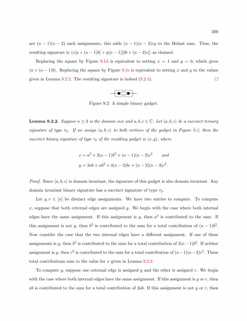
200

are (κ − 1)(κ − 2) such assignments, this adds (κ − 1)(κ − 2)cy to the Holant sum. Thus, the

resulting signature is 〈x[a+ (κ− 1)b] + y(κ− 1)[2b+ (κ− 2)c]〉 as claimed.

Replacing the square by Figure 9.1d is equivalent to setting x = 1 and y = 0, which gives

〈a + (κ − 1)b〉. Replacing the square by Figure 9.1e is equivalent to setting x and y to the values

given in Lemma 9.2.2. The resulting signature is indeed (9.2.4).

Figure 9.2: A simple binary gadget.

Lemma 9.2.2. Suppose κ ≥ 3 is the domain size and a, b, c ∈ C. Let 〈a, b, c〉 be a succinct ternary

signature of type τ3. If we assign 〈a, b, c〉 to both vertices of the gadget in Figure 9.2, then the

succinct binary signature of type τ2 of the resulting gadget is 〈x, y〉, where

x = a2 + 3(κ− 1)b2 + (κ− 1)(κ− 2)c2 and

y = 2ab+ κb2 + 4(κ− 2)bc+ (κ− 2)(κ− 3)c2.

Proof. Since 〈a, b, c〉 is domain invariant, the signature of this gadget is also domain invariant. Any

domain invariant binary signature has a succinct signature of type τ2.

Let g, r ∈ [κ] be distinct edge assignments. We have two entries to compute. To compute

x, suppose that both external edges are assigned g. We begin with the case where both internal

edges have the same assignment. If this assignment is g, then a2 is contributed to the sum. If

this assignment is not g, then b2 is contributed to the sum for a total contribution of (κ − 1)b2.

Now consider the case that the two internal edges have a different assignment. If one of these

assignments is g, then b2 is contributed to the sum for a total contribution of 2(κ− 1)b2. If neither

assignment is g, then c2 is contributed to the sum for a total contribution of (κ−1)(κ−2)c2. These

total contributions sum to the value for x given in Lemma 9.2.2.

To compute y, suppose one external edge is assigned g and the other is assigned r. We begin

with the case where both internal edges have the same assignment. If this assignment is g or r, then

ab is contributed to the sum for a total contribution of 2ab. If this assignment is not g or r, then

201

b2 is contributed to the sum for a total contribution of (κ − 2)b2. Now consider the case that the

two internal edges have a different assignment. If both are assigned g or r, then b2 is contributed

to the sum for a total contribution of 2b2. If exactly one is assigned g or r, then bc is contributed

to the sum for a total contribution of 4(κ−2)bc. If neither is assigned g or r, then c3 is contributed

to the sum for a total contribution of (κ− 2)(κ− 3)c3. These total contributions sum to the value

for y given in Lemma 9.2.2.

When checking these proofs, a concern is that some assignments might not have been counted

(or maybe some assignment was counted twice). A sanity check to address this concern is to set

a = b = c = 1 and inspect the resulting expression. If computed correctly, the result will be κm,

where m is the number of internal edges, which is the number of internal edge assignments.

Figure 9.3: A simple quaternary gadget.

Lemma 9.2.3. Suppose κ ≥ 3 is the domain size and a, b, c ∈ C. Let 〈a, b, c〉 be a succinct ternary

signature of type τ3. If we assign 〈a, b, c〉 to both vertices of the gadget in Figure 9.3, then the

succinct quaternary signature of type τ4 of the resulting gadget is

f =⟨f 1 1

1 1, f 1 2

1 1, f 1 2

1 2, f 1 3

1 2, f 1 2

2 1, f 1 3

2 1, f 1 1

2 2, f 1 1

2 3, f 1 4

2 3

⟩,

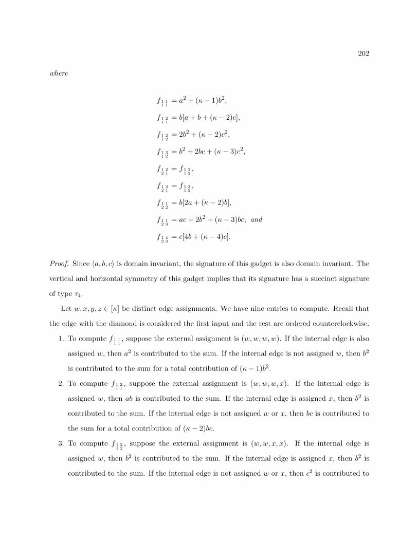
202

where

f 1 11 1

= a2 + (κ− 1)b2,

f 1 21 1

= b[a+ b+ (κ− 2)c],

f 1 21 2

= 2b2 + (κ− 2)c2,

f 1 31 2

= b2 + 2bc+ (κ− 3)c2,

f 1 22 1

= f 1 21 2,

f 1 32 1

= f 1 31 2,

f 1 12 2

= b[2a+ (κ− 2)b],

f 1 12 3

= ac+ 2b2 + (κ− 3)bc, and

f 1 42 3

= c[4b+ (κ− 4)c].

Proof. Since 〈a, b, c〉 is domain invariant, the signature of this gadget is also domain invariant. The

vertical and horizontal symmetry of this gadget implies that its signature has a succinct signature

of type τ4.

Let w, x, y, z ∈ [κ] be distinct edge assignments. We have nine entries to compute. Recall that

the edge with the diamond is considered the first input and the rest are ordered counterclockwise.

1. To compute f 1 11 1

, suppose the external assignment is (w,w,w,w). If the internal edge is also

assigned w, then a2 is contributed to the sum. If the internal edge is not assigned w, then b2

is contributed to the sum for a total contribution of (κ− 1)b2.

2. To compute f 1 21 1

, suppose the external assignment is (w,w,w, x). If the internal edge is

assigned w, then ab is contributed to the sum. If the internal edge is assigned x, then b2 is

contributed to the sum. If the internal edge is not assigned w or x, then bc is contributed to

the sum for a total contribution of (κ− 2)bc.

3. To compute f 1 21 2

, suppose the external assignment is (w,w, x, x). If the internal edge is

assigned w, then b2 is contributed to the sum. If the internal edge is assigned x, then b2 is

contributed to the sum. If the internal edge is not assigned w or x, then c2 is contributed to

203

the sum for a total contribution of (κ− 2)c2.

4. To compute f 1 31 2

, suppose the external assignment is (w,w, x, y). If the internal edge is

assigned w, then b2 is contributed to the sum. If the internal edge is assigned x, then bc is

contributed to the sum. If the internal edge is assigned y, then bc is contributed to the sum.

If the internal edge is not assigned w, x or y, then c2 is contributed to the sum for a total

contribution of (κ− 3)c2.

5. To compute f 1 31 2

, suppose the external assignment is (w, x,w, x). This entry is the same as

that for (w,w, x, x). The reason is that the signature is unchanged if the two external edges

of the lower vertex are swapped since 〈a, b, c〉 is symmetric.

6. To compute f 1 32 1

, suppose the external assignment is (w, x,w, y). This entry is the same as

that for (w,w, x, y) for the same reason as the previous entry.

7. To compute f 1 12 2

, suppose the external assignment is (w, x, x, w). If the internal edge is

assigned w, then ab is contributed to the sum. If the internal edge is assigned x, then ab is

contributed to the sum. If the internal edge is not assigned w or x, then b2 is contributed to

the sum for a total contribution of (κ− 2)b2.

8. To compute f 1 12 3

, suppose the external assignment is (w, x, y, w). If the internal edge is

assigned w, then ac is contributed to the sum. If the internal edge is assigned x, then b2 is

contributed to the sum. If the internal edge is assigned y, then b2 is contributed to the sum.

If the internal edge is not assigned w, x or y, then bc is contributed to the sum for a total

contribution of (κ− 3)c2.

9. To compute f 1 42 3

, suppose the external assignment is (w, x, y, z). If the internal edge is assigned

w, x, y, or z, then bc is contributed to the sum for a total contribution of 4bc. If the internal

edge is not assigned w, x, y or z, then c2 is contributed to the sum for a total contribution of

(κ− 4)c2.

These total contributions each sum to their corresponding entry of f given in the statement of

Lemma 9.2.3.

Although possible, it would be difficult to compute the signature of the gadget in Figure 9.4c

through partitioning of the internal edge assignments alone. To simplify matters, we utilize the

204

calculations from Lemma 9.2.3. Since composing the gadget in Figure 9.4a with the one in Fig-

ure 9.4b gives a symmetric signature, we refrain from distinguishing the external edges of the gadget

in Figure 9.4b.

(a) Inner structure (b) Outer structure (c) Entire binary gadget

Figure 9.4: Decomposition of a ternary gadget. All circle vertices are assigned 〈a, b, c〉and the square vertex in (b) is assigned the signature of the gadget in (a).

Lemma 9.2.4. Suppose κ ≥ 3 is the domain size and a, b, c ∈ C. Let 〈a, b, c〉 be a succinct ternary

signature of type τ3. If we assign 〈a, b, c〉 to all vertices of the gadget in Figure 9.4c, then the

succinct ternary signature of type τ3 of the resulting gadget is 〈a′, b′, c′〉, where

a′ = a3 + 3(κ− 1)ab2 + 4(κ− 1)b3 + 3(κ− 1)(κ− 2)(b2c+ bc2) + (κ− 1)(κ− 2)(κ− 3)c3,

b′ = a2b+ 4ab2 + 2(κ− 2)abc+ (κ− 2)ac2 + (5κ− 7)b3 + (κ− 2)(κ+ 5)b2c

+ (κ− 2)(7κ− 18)bc2 + (κ− 2)(κ− 3)2c3, and

c′ = 3ab2 + 6abc+ 3(κ− 3)ac2 + (κ+ 5)b3 + 3(7κ− 18)b2c+ 9(κ− 3)2bc2

+ (κ3 − 9κ2 + 29κ− 32)c3.

Furthermore, if A = 0, then

a′ = 3b′ − 2c′,

b′ = (5κ+ 14)b3 + (κ2 + 9κ− 42)b2c+ (7κ2 − 33κ+ 42)bc2 + (κ− 2)(κ2 − 6κ+ 7)c3, and

c′ = (κ+ 14)b3 + 21(κ− 2)b2c+ 3(3κ2 − 15κ+ 14)bc2 + (κ3 − 9κ2 + 23κ− 14)c3.

Proof. Since 〈a, b, c〉 is domain invariant, the signature of this gadget is also domain invariant. As

a ternary signature, the rotational symmetry of this gadget implies the symmetry of the signature.

205

Any symmetric domain invariant ternary signature has a succinct signature of type τ3.

Consider the gadget in Figure 9.4a. We assign 〈a, b, c〉 to both vertices. Then by Lemma 9.2.3,

the succinct quaternary signature of this gadget is the signature f given in Lemma 9.2.3.

Now consider the gadget in Figure 9.4b. We assign 〈a, b, c〉 to the circle vertex and f to the

square vertex. The resulting gadget is the one in Figure 9.4c, which is symmetric. Thus, there is

no need to distinguish the external edges. We have three entries to compute.

Let g, r, y ∈ [κ] be distinct edge assignments. To compute a′, suppose that all external edges

are assigned g. We begin with the case where both internal edges have the same assignment. If

this assignment is g, then af 1 11 1

is contributed to the sum. If this assignment is not g, then bf 1 21 2

is contributed to the sum for a total contribution of (κ − 1)bf 1 21 2

. Now consider the case that

the two internal edges have a different assignment. If one of these assignments is g, then bf 1 21 1

is

contributed to the sum for a total contribution of 2(κ − 1)bf 1 21 1

. If neither assignment is g, then

cf 1 31 2

is contributed to the sum for a total contribution of (κ − 1)(κ − 2)cf 1 31 2

. After substituting

for the entries of f , these total contributions sum to the value for a′ given in Lemma 9.2.4.

To compute b′, suppose the left external edges are assigned g and the right external edge is

assigned r. We begin with the case where both internal edges have the same assignment. If

this assignment is g, then bf 1 11 1

is contributed to the sum. If this assignment is r, then af 1 21 2

is

contributed to the sum. If this assignment is not g or r, then bf 1 21 2

is contributed to the sum for

a total contribution of (κ − 2)bf 1 21 2

. Now consider the case that the two internal edges have a

different assignments. If both are assigned g or r, then bf 1 21 1

is contributed to the sum for a total

contribution of 2bf 1 21 1

. If one is assigned g and the other is not assigned r, then cf 1 21 1

is contributed

to the sum for a total contribution of 2(κ − 2)cf 1 21 1

. If one is assigned r and the other is not

assigned g, then bf 1 31 2

is contributed to the sum for a total contribution of 2(κ− 2)bf 1 31 2

. If neither

is assigned g or r, then cf 1 31 2

is contributed to the sum for a total contribution of (κ−2)(κ−3)cf 1 31 2

.

After substituting for the entries of f , these total contributions sum to the value for b′ given in

Lemma 9.2.4.

To compute c′, suppose the upper-left external edge is assigned g, the lower-left external edge

is assigned r, and the right external edge is assigned y. We begin with the case where both internal

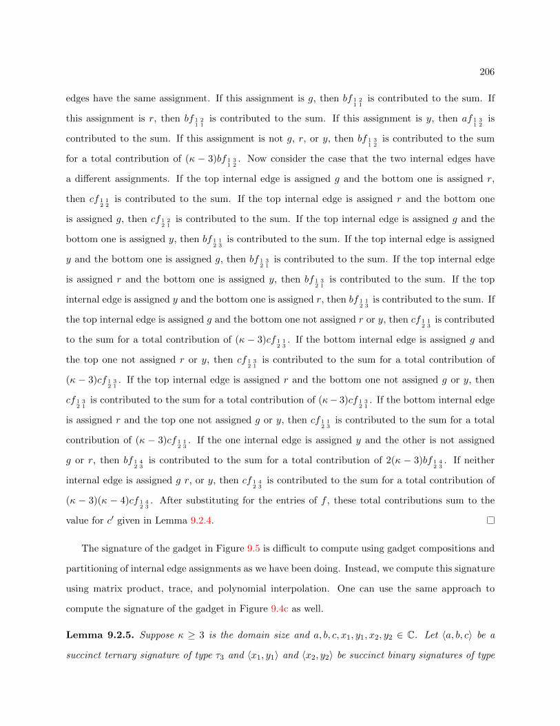
206

edges have the same assignment. If this assignment is g, then bf 1 21 1

is contributed to the sum. If

this assignment is r, then bf 1 21 1

is contributed to the sum. If this assignment is y, then af 1 31 2

is

contributed to the sum. If this assignment is not g, r, or y, then bf 1 31 2

is contributed to the sum

for a total contribution of (κ − 3)bf 1 31 2

. Now consider the case that the two internal edges have

a different assignments. If the top internal edge is assigned g and the bottom one is assigned r,

then cf 1 12 2

is contributed to the sum. If the top internal edge is assigned r and the bottom one

is assigned g, then cf 1 22 1

is contributed to the sum. If the top internal edge is assigned g and the

bottom one is assigned y, then bf 1 12 3

is contributed to the sum. If the top internal edge is assigned

y and the bottom one is assigned g, then bf 1 32 1

is contributed to the sum. If the top internal edge

is assigned r and the bottom one is assigned y, then bf 1 32 1

is contributed to the sum. If the top

internal edge is assigned y and the bottom one is assigned r, then bf 1 12 3

is contributed to the sum. If

the top internal edge is assigned g and the bottom one not assigned r or y, then cf 1 12 3

is contributed

to the sum for a total contribution of (κ − 3)cf 1 12 3

. If the bottom internal edge is assigned g and

the top one not assigned r or y, then cf 1 32 1

is contributed to the sum for a total contribution of

(κ − 3)cf 1 32 1

. If the top internal edge is assigned r and the bottom one not assigned g or y, then

cf 1 32 1

is contributed to the sum for a total contribution of (κ− 3)cf 1 32 1

. If the bottom internal edge

is assigned r and the top one not assigned g or y, then cf 1 12 3

is contributed to the sum for a total

contribution of (κ − 3)cf 1 12 3

. If the one internal edge is assigned y and the other is not assigned

g or r, then bf 1 42 3

is contributed to the sum for a total contribution of 2(κ − 3)bf 1 42 3

. If neither

internal edge is assigned g r, or y, then cf 1 42 3

is contributed to the sum for a total contribution of

(κ − 3)(κ − 4)cf 1 42 3

. After substituting for the entries of f , these total contributions sum to the

value for c′ given in Lemma 9.2.4.

The signature of the gadget in Figure 9.5 is difficult to compute using gadget compositions and

partitioning of internal edge assignments as we have been doing. Instead, we compute this signature

using matrix product, trace, and polynomial interpolation. One can use the same approach to

compute the signature of the gadget in Figure 9.4c as well.

Lemma 9.2.5. Suppose κ ≥ 3 is the domain size and a, b, c, x1, y1, x2, y2 ∈ C. Let 〈a, b, c〉 be a

succinct ternary signature of type τ3 and 〈x1, y1〉 and 〈x2, y2〉 be succinct binary signatures of type

207

Figure 9.5: A more complicated binary gadget.

τ2. If to the gadget in Figure 9.5 we assign 〈a, b, c〉 to the circle vertices, 〈x1, y1〉 to the square

vertex, and 〈x2, y2〉 to the triangle vertex, then the succinct binary signature of type τ2 of the

resulting gadget is 〈x, y〉, where

x = x1x2a2 + 2(κ− 1)(x1y2 + x2y1 + y1y2)ab+ 2(κ− 1)(κ− 2)y1y2ac

+ (κ− 1)[3x1x2 + κ(x1y2 + x2y1) + (7κ− 12)y1y2]b2

+ 2(κ− 1)(κ− 2)[2(x1y2 + x2y1) + (3κ− 7)y1y2]bc

+ (κ− 1)(κ− 2)[x1x2 + (κ− 3)(x1y2 + x2y1) + (κ2 − 5κ+ 7)y1y2]c2 and

y = y1y2a2 + 2[x1x2 + x1y2 + x2y1 + 3(κ− 2)y1y2]ab+ 2(κ− 2)[x1y2 + x2y1 + (κ− 3)y1y2]ac

+ [κx1x2 + (7κ− 12)(x1y2 + x2y1) + 3(3κ2 − 11κ+ 11)y1y2]b2

+ 2(κ− 2)[2x1x2 + (3κ− 7)(x1y2 + x2y1) + 3(κ2 − 4κ+ 5)y1y2]bc

+ (κ− 2)[(κ− 3)x1x2 + (κ2 − 5κ+ 7)(x1y2 + x2y1) + (κ3 − 6κ2 + 14κ− 13)]c2.

Furthermore, if 〈x1, y1〉 = 1κ〈ω

r + κ− 1, ωr − 1〉 and 〈x2, y2〉 = 1κ〈ω

s + κ− 1, ωs − 1〉, then

x =B2

κ2

[Φωr+s + (κ− 1)(ωr + ωs + Ψ + 1)

]and y =

B2

κ2

[Φωr+s − (ωr + ωs + Ψ + 1) + κ

],

where Φ = C2

B2 and Ψ = (κ−2)A2

B2 .

Proof. Since 〈a, b, c〉, 〈x1, y1〉, and 〈x2, y2〉 are domain invariant, the signature of this gadget is also

domain invariant. Any domain invariant binary signature has a succinct signature of type τ2.

We compute a′, b′, and c′ using the algorithm for Holantκ(F) when every non-degenerate

signature in F is of arity at most 2, which is to use matrix product and trace. Then we finish with

208

polynomial interpolation. Let Mκ(t) be a κ-by-κ matrix such that

(Mκ(t))i,j =

a i = j = t

b i = j 6= t

b i 6= j and (i = t or j = t)

c otherwise.

For example, M4(1) =

[a b b bb b c cb c b cb c c b

]. If we fix an input of 〈a, b, c〉 to t ∈ [κ], then the resulting binary

signature (which is no longer domain invariant) has the signature matrix Mκ(t).

Consider x and y as polynomials in κ with coefficients in Z[a, b, c, x1, y1, x2, y2]. Then

x(κ) = tr(Mκ(1)

[y1Jκ + (x1 − y1)Iκ

]Mκ(1)

[y2Jκ + (x2 − y2)Iκ

])and

y(κ) = tr(Mκ(1)

[y1Jκ + (x1 − y1)Iκ

]Mκ(2)

[y2Jκ + (x2 − y2)Iκ

]).

Since there are just four internal edges in this gadget, both of x(κ) and y(κ) are of degree at most 4

in κ. Therefore, we interpolate each of these polynomials using their evaluations at 3 ≤ κ ≤ 7 and

obtain the expressions for x and y given in Lemma 9.2.5.

Remark. Lemma 9.2.2 is the special case of Lemma 9.2.5 with 〈x1, y1〉 = 〈x2, y2〉 = 〈1, 0〉.

In order to apply a holographic transformation on a particular signature, it is convenient to

express the signature as a sum of degenerate signatures. Let eκ,i be the standard basis vector of

length κ with a 1 at location i and 0 elsewhere. Also let 1κ be the all 1’s vector of length κ. Then

209

the succinct ternary signature 〈a, b, c〉 on domain size κ can be expressed as

〈a, b, c〉 = c1⊗3κ + (a− c)

κ∑i=1

e⊗3κ,i + (b− c)

∑i,j∈[κ]i 6=j

eκ,i ⊗ eκ,i ⊗ eκ,j

+ eκ,i ⊗ eκ,j ⊗ eκ,i

+ eκ,j ⊗ eκ,i ⊗ eκ,i

(9.2.5)

= b1⊗3κ + (a− b)

κ∑i=1

e⊗3κ,i + (c− b)

∑σ:1,2,3→[κ]σ injective

eκ,σ(1) ⊗ eκ,σ(2) ⊗ eκ,σ(3). (9.2.6)

The expression in (9.2.5) contains 1 + κ + 3κ(κ − 1) = 3κ2 − 2κ + 1 summands. In general, this

is smaller than the one in (9.2.6), which contains 1 + κ + κ(κ − 1)(κ − 2) = κ3 − 3κ2 + 3κ + 1

summands. It is advantageous to find an expression that minimizes the number of summands. This

leads to less computation in the proof of Lemma 9.2.6. However, determining the fewest number

of summands for a given signature is exactly the problem of determining tensor rank, which is a

problem well-known to be difficult [76].

Figure 9.6: Local holographic transformation gadget construction for a ternary signa-ture.

There is a gadget construction that mimics the behavior of a holographic transformation. This

construction is called a local holographic transformation [53]. For x, y ∈ C, let 〈x, y〉 be a succinct

binary signature of type τ2. Consider the gadget in Figure 9.6. If we assign 〈a, b, c〉 to the circle

vertex and 〈x, y〉 to the square vertex, then the resulting signature of this gadget is the same as

applying a holographic transformation on 〈a, b, c〉 with basis T = yJκ + (x− y)Iκ. We use this fact

in the following proof.

Lemma 9.2.6. Suppose κ ≥ 3 is the domain size and a, b, c, x, y ∈ C. Let 〈a, b, c〉 be a succinct

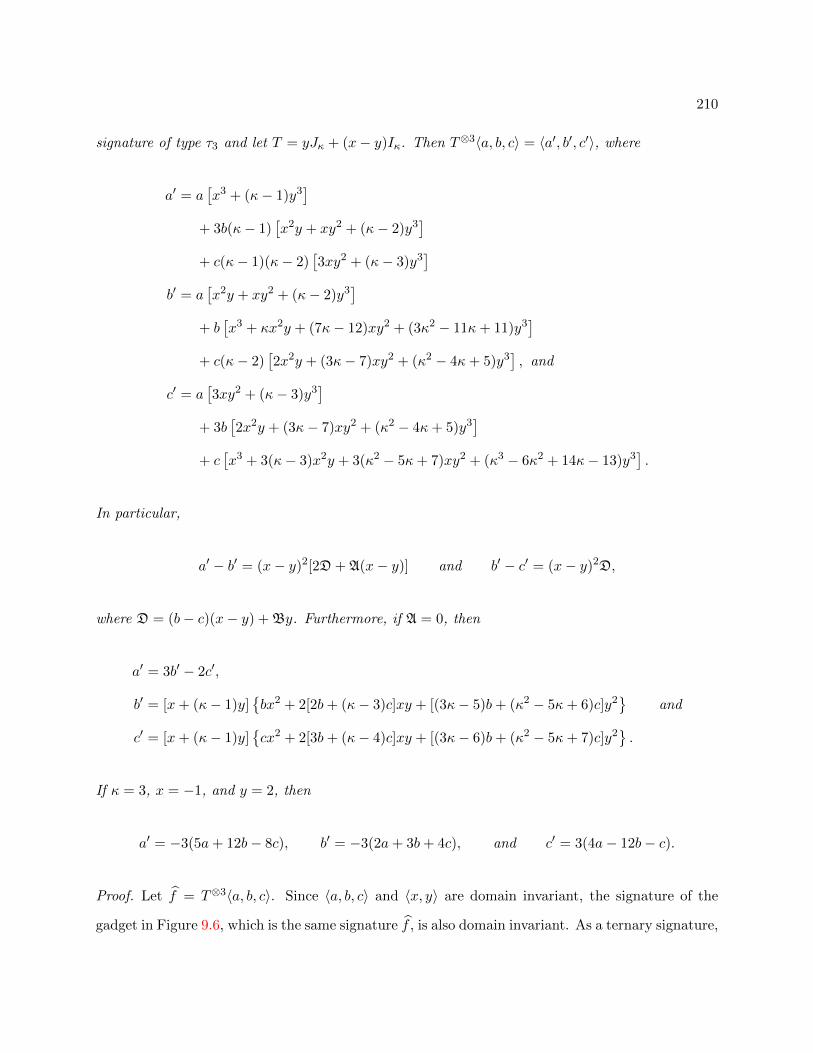
210

signature of type τ3 and let T = yJκ + (x− y)Iκ. Then T⊗3〈a, b, c〉 = 〈a′, b′, c′〉, where

a′ = a[x3 + (κ− 1)y3

]+ 3b(κ− 1)

[x2y + xy2 + (κ− 2)y3

]+ c(κ− 1)(κ− 2)

[3xy2 + (κ− 3)y3

]b′ = a

[x2y + xy2 + (κ− 2)y3

]+ b

[x3 + κx2y + (7κ− 12)xy2 + (3κ2 − 11κ+ 11)y3

]+ c(κ− 2)

[2x2y + (3κ− 7)xy2 + (κ2 − 4κ+ 5)y3

], and

c′ = a[3xy2 + (κ− 3)y3

]+ 3b

[2x2y + (3κ− 7)xy2 + (κ2 − 4κ+ 5)y3

]+ c

[x3 + 3(κ− 3)x2y + 3(κ2 − 5κ+ 7)xy2 + (κ3 − 6κ2 + 14κ− 13)y3

].

In particular,

a′ − b′ = (x− y)2[2D + A(x− y)] and b′ − c′ = (x− y)2D,

where D = (b− c)(x− y) + By. Furthermore, if A = 0, then

a′ = 3b′ − 2c′,

b′ = [x+ (κ− 1)y]bx2 + 2[2b+ (κ− 3)c]xy + [(3κ− 5)b+ (κ2 − 5κ+ 6)c]y2

and

c′ = [x+ (κ− 1)y]cx2 + 2[3b+ (κ− 4)c]xy + [(3κ− 6)b+ (κ2 − 5κ+ 7)c]y2

.

If κ = 3, x = −1, and y = 2, then

a′ = −3(5a+ 12b− 8c), b′ = −3(2a+ 3b+ 4c), and c′ = 3(4a− 12b− c).

Proof. Let f = T⊗3〈a, b, c〉. Since 〈a, b, c〉 and 〈x, y〉 are domain invariant, the signature of the

gadget in Figure 9.6, which is the same signature f , is also domain invariant. As a ternary signature,

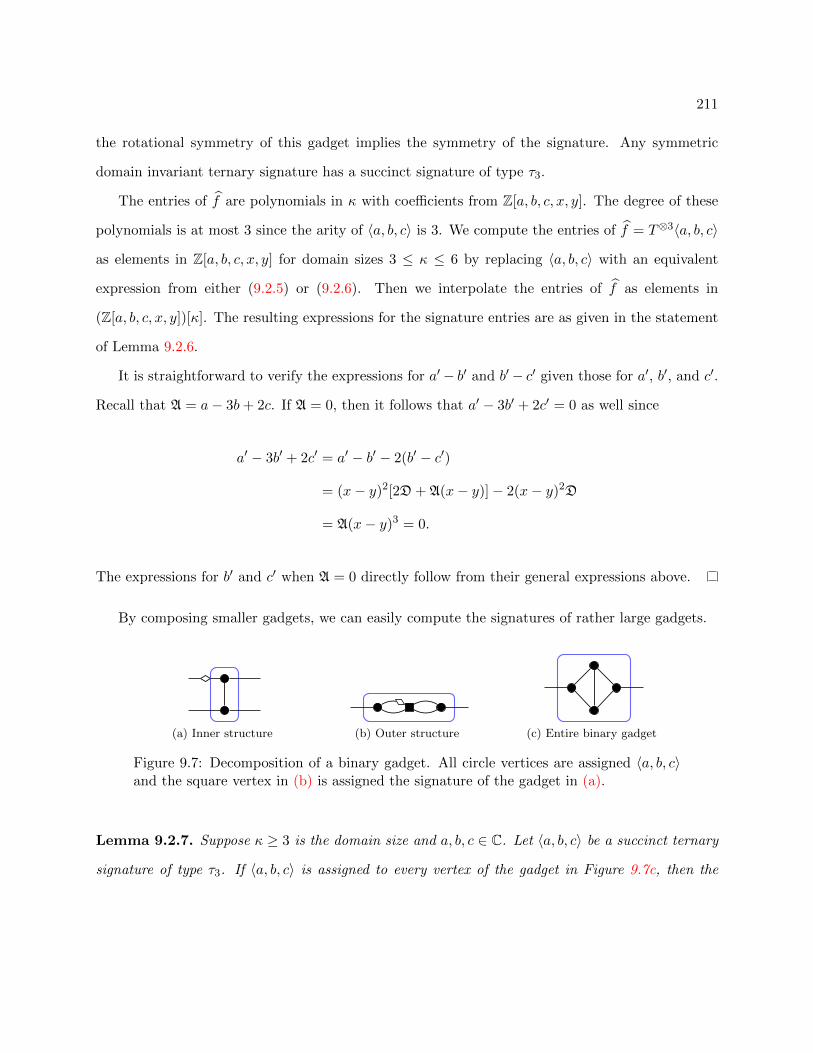
211

the rotational symmetry of this gadget implies the symmetry of the signature. Any symmetric

domain invariant ternary signature has a succinct signature of type τ3.

The entries of f are polynomials in κ with coefficients from Z[a, b, c, x, y]. The degree of these

polynomials is at most 3 since the arity of 〈a, b, c〉 is 3. We compute the entries of f = T⊗3〈a, b, c〉

as elements in Z[a, b, c, x, y] for domain sizes 3 ≤ κ ≤ 6 by replacing 〈a, b, c〉 with an equivalent

expression from either (9.2.5) or (9.2.6). Then we interpolate the entries of f as elements in

(Z[a, b, c, x, y])[κ]. The resulting expressions for the signature entries are as given in the statement

of Lemma 9.2.6.

It is straightforward to verify the expressions for a′− b′ and b′− c′ given those for a′, b′, and c′.

Recall that A = a− 3b+ 2c. If A = 0, then it follows that a′ − 3b′ + 2c′ = 0 as well since

a′ − 3b′ + 2c′ = a′ − b′ − 2(b′ − c′)

= (x− y)2[2D + A(x− y)]− 2(x− y)2D

= A(x− y)3 = 0.

The expressions for b′ and c′ when A = 0 directly follow from their general expressions above.

By composing smaller gadgets, we can easily compute the signatures of rather large gadgets.

(a) Inner structure (b) Outer structure (c) Entire binary gadget

Figure 9.7: Decomposition of a binary gadget. All circle vertices are assigned 〈a, b, c〉and the square vertex in (b) is assigned the signature of the gadget in (a).

Lemma 9.2.7. Suppose κ ≥ 3 is the domain size and a, b, c ∈ C. Let 〈a, b, c〉 be a succinct ternary

signature of type τ3. If 〈a, b, c〉 is assigned to every vertex of the gadget in Figure 9.7c, then the

212

resulting signature is the succinct binary signature 〈x, y〉 of type τ2, where

x = a4 + 6(κ− 1)a2b2 + 16(κ− 1)ab3 + 12(κ− 1)(κ− 2)ab2c+ 12(κ− 1)(κ− 2)abc2

+ 4(κ− 1)(κ− 2)(κ− 3)ac3 + 3(κ− 1)(5κ− 7)b4 + 4(κ− 1)(κ− 2)(κ+ 5)b3c

+ 6(κ− 1)(κ− 2)(7κ− 18)b2c2 + 12(κ− 3)2(κ− 1)(κ− 2)bc3

+ (κ− 1)(κ− 2)(κ3 − 9κ2 + 29κ− 32)c4 and

y = 2a3b+ (κ+ 4)a2b2 + 4(κ− 2)a2bc+ (κ− 2)a2c2 + 2(9κ− 11)ab3 + 2(κ− 2)(3κ+ 8)ab2c

+ 2(κ− 2)(12κ− 31)abc2 + 2(κ− 2)(2κ2 − 11κ+ 16)ac3 + (7κ2 + 3κ− 24)b4

+ 2(κ− 2)(κ2 + 31κ− 70)b3c+ (κ− 2)(48κ2 − 234κ+ 301)b2c2

+ 2(κ− 2)(6κ3 − 45κ2 + 121κ− 116)bc3 + (κ− 2)(κ− 3)(κ3 − 7κ2 + 19κ− 20)c4.

Proof. Since 〈a, b, c〉 is domain invariant, the signature of this gadget is also domain invariant. Any

domain invariant binary signature has a succinct signature of type τ2.

Consider the gadget in Figure 9.7a. We assign 〈a, b, c〉 to both vertices. By Lemma 9.2.3, this

gadget has the succinct quaternary signature f of type τ4, where f is given in Lemma 9.2.3.

Now consider the gadget in Figure 9.7b. We assign 〈a, b, c〉 the circle vertices and f to the

square vertex. By partitioning the internal edge assignments into parts with the same contribution

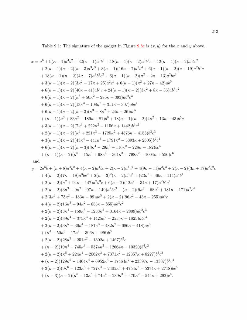
213

Table 9.1: The signature of the gadget in Figure 9.8c is 〈x, y〉 for the x and y above.

x = a6 + 9(κ− 1)a4b2 + 32(κ− 1)a3b3 + 18(κ− 1)(κ− 2)a3b2c+ 12(κ− 1)(κ− 2)a3bc2

+ 2(κ− 1)(κ− 2)(κ− 3)a3c3 + 3(κ− 1)(16κ− 7)a2b4 + 6(κ− 1)(κ− 2)(κ+ 19)a2b3c

+ 18(κ− 1)(κ− 2)(4κ− 7)a2b2c2 + 6(κ− 1)(κ− 2)(κ2 + 2κ− 13)a2bc3

+ 3(κ− 1)(κ− 2)(3κ2 − 17κ+ 25)a2c4 + 6(κ− 1)(κ2 + 27κ− 42)ab5

+ 6(κ− 1)(κ− 2)(40κ− 41)ab4c+ 24(κ− 1)(κ− 2)(3κ2 + 8κ− 36)ab3c2

+ 6(κ− 1)(κ− 2)(κ3 + 50κ2 − 285κ+ 393)ab2c3

+ 6(κ− 1)(κ− 2)(13κ3 − 108κ2 + 311κ− 307)abc4

+ 6(κ− 1)(κ− 2)(κ− 3)(κ3 − 8κ2 + 24κ− 26)ac5

+ (κ− 1)(κ3 + 83κ2 − 189κ+ 81)b6 + 18(κ− 1)(κ− 2)(4κ2 + 13κ− 43)b5c

+ 3(κ− 1)(κ− 2)(7κ3 + 222κ2 − 1156κ+ 1442)b4c2

+ 2(κ− 1)(κ− 2)(κ4 + 221κ3 − 1725κ2 + 4576κ− 4153)b3c3

+ 3(κ− 1)(κ− 2)(43κ4 − 441κ3 + 1791κ2 − 3393κ+ 2505)b2c4

+ 6(κ− 1)(κ− 2)(κ− 3)(3κ4 − 29κ3 + 116κ2 − 228κ+ 182)bc5

+ (κ− 1)(κ− 2)(κ6 − 15κ5 + 98κ4 − 361κ3 + 798κ2 − 1004κ+ 556)c6

and

y = 2a5b+ (κ+ 8)a4b2 + 4(κ− 2)a4bc+ 2(κ− 2)a4c2 + 4(9κ− 11)a3b3 + 2(κ− 2)(3κ+ 17)a3b2c

+ 4(κ− 2)(7κ− 18)a3bc2 + 2(κ− 3)2(κ− 2)a3c3 + (23κ2 + 49κ− 114)a2b4

+ 2(κ− 2)(κ2 + 94κ− 147)a2b3c+ 6(κ− 2)(12κ2 − 34κ+ 17)a2b2c2

+ 2(κ− 2)(3κ3 + 9κ2 − 97κ+ 149)a2bc3 + (κ− 2)(9κ3 − 68κ2 + 181κ− 171)a2c4

+ 2(3κ3 + 73κ2 − 183κ+ 99)ab5 + 2(κ− 2)(96κ2 − 43κ− 255)ab4c

+ 4(κ− 2)(16κ3 + 94κ2 − 655κ+ 855)ab3c2

+ 2(κ− 2)(3κ4 + 159κ3 − 1233κ2 + 3164κ− 2809)ab2c3

+ 2(κ− 2)(39κ4 − 375κ3 + 1425κ2 − 2555κ+ 1825)abc4

+ 2(κ− 2)(3κ5 − 36κ4 + 181κ3 − 482κ2 + 686κ− 418)ac5

+ (κ4 + 50κ3 − 17κ2 − 396κ+ 486)b6

+ 2(κ− 2)(28κ3 + 251κ2 − 1302κ+ 1467)b5c

+ (κ− 2)(19κ4 + 745κ3 − 5374κ2 + 12664κ− 10320)b4c2

+ 2(κ− 2)(κ5 + 224κ4 − 2062κ3 + 7371κ2 − 12357κ+ 8227)b3c3

+ (κ− 2)(129κ5 − 1464κ4 + 6952κ3 − 17464κ2 + 23397κ− 13387)b2c4

+ 2(κ− 2)(9κ6 − 123κ5 + 727κ4 − 2405κ3 + 4754κ2 − 5374κ+ 2718)bc5

+ (κ− 3)(κ− 2)(κ6 − 13κ5 + 74κ4 − 239κ3 + 470κ2 − 544κ+ 292)c6.

214

to the sum, one can verify that this gadget has the succinct binary signature 〈x, y〉 of type τ2, where

x = f 1 11 1

[a2 + (κ− 1)b2

]+ 4(κ− 1)f 1 2

1 1

[ab+ b2 + (κ− 2)bc

]+ (κ− 1)f 1 2

1 2

[2ab+ (κ− 2)b2

]+ 2(κ2 − 3κ+ 2)f 1 3

1 2

[ac+ 2b2 + (κ− 3)bc

]+ (κ− 1)f 1 2

2 1

[2b2 + (κ− 2)c2

]+ 2(κ2 − 3κ+ 2)f 1 3

2 1

[b2 + 2bc+ (κ− 3)c2

]+ (κ− 1)f 1 1

2 2

[2b2 + (κ− 2)c2

]+ 2(κ2 − 3κ+ 2)f 1 1

2 3

[b2 + 2bc+ (κ− 3)c2

]+ (κ3 − 6κ2 + 11κ− 6)f 1 4

2 3

[4bc+ (κ− 4)c2

]and

y = f 1 11 1

[2ab+ (κ− 2)b2

]+ 4f 1 2

1 1

[ab+ (κ− 2)ac+ (2κ− 3)b2 + (κ− 2)2bc

]+f 1 2

1 2

[a2 + 2(κ− 2)ab+ (κ2 − 3κ+ 3)b2

]+ 2(κ− 2)f 1 3

1 2

[2ab+ (κ− 3)ac+ 2(κ− 2)b2 + (κ2 − 4κ+ 5)bc

]+f 1 2

2 1

[2b2 + 4(κ− 2)bc+ (κ2 − 5κ+ 6)c2

]+ 2(κ− 2)f 1 3

2 1

[3b2 + 2(2κ− 5)bc+ (κ2 − 5κ+ 7)c2

]+f 1 1

2 2

[2b2 + 4(κ− 2)bc+ (κ2 − 5κ+ 6)c2

]+ 2(κ− 2)f 1 1

2 3

[3b2 + 2(2κ− 5)bc+ (κ2 − 5κ+ 7)c2

]+ (κ2 − 5κ+ 6)f 1 4

2 3

[4b2 + 4(κ− 3)bc+ (κ2 − 5κ+ 8)c2

].

Substituting for the entries of f gives the result stated in Lemma 9.2.7.

Lemma 9.2.8. Suppose κ ≥ 3 is the domain size and a, b, c ∈ C. Let 〈a, b, c〉 be a succinct ternary

signature of type τ3. If 〈a, b, c〉 is assigned to every vertex of the gadget in Figure 9.8c, then the

resulting signature is the binary succinct signature 〈x, y〉 of type τ2, where x and y are given in

Table 9.1.

215

(a) Inner structure (b) Outer structure (c) Entire binary gadget

Figure 9.8: Decomposition of a binary gadget. All circle vertices are assigned 〈a, b, c〉and the triangle vertices in (b) is assigned the signature of the gadget in (a).

Proof. Since 〈a, b, c〉 is domain invariant, the signature of this gadget is also domain invariant. Any

domain invariant binary signature has a succinct signature of type τ2.

Consider the gadget in Figure 9.8a. We assign 〈a, b, c〉 to all vertices. By Lemma 9.2.4, this

gadget has the succinct ternary signature f = 〈a0, b0, c0〉 of type τ4, where a0, b0, and c0 are given

in the statement of Lemma 9.2.4 as a′, b′, and c′ respectively.

Now consider the gadget in Figure 9.8b. We assign f to the vertices. By Lemma 9.2.2, the

resulting gadget has the binary succinct signature 〈x, y〉 of type τ2, where

x = a20 + 3(κ− 1)b20 + (κ− 1)(κ− 2)c2

0 and

y = 2a0b0 + κb20 + 4(κ− 2)b0c0 + (κ− 2)(κ− 3)c20.

Substituting for a0, b0, and c0 gives the result in Table 9.1.

Beyond the gadgets in this section, there are two 9-by-9 recurrence matrices that appear in our

proofs in Chapter 11 (see Table 11.1 and Table 11.3). No entry in those recurrence matrices is any

harder to compute than any signature entry appearing in this section. The difficulty with these

recurrence matrices is the sheer number of terms that must be computed.

216

Chapter 10

Dichotomy for Counting Edge

Colorings over Planar Regular Graphs

In this chapter, we prove that counting edge colorings using κ colors is #P-hard over planar r-

regular graphs for all κ ≥ r ≥ 3. The problem is polynomial-time computable in all other parameter

settings. We reduce from evaluating the Tutte polynomial of a planar graph. If κ = r, then we

reduce from the point (κ+ 1, κ+ 1). If κ > r, then we reduce from the point (1−κ, 0), which is the

problem of counting vertex colorings using κ colors. To express our reductions, we introduce notion

to succinctly represent signatures with duplicate entries. This work was published in [32, 33].

10.1 Background

An edge κ-coloring of a graph G is a labeling of the edges of G with colors such that any two

adjacent edges have different colors. A fundamental problem in graph theory is to determine how

many colors are required to edge color a graph G. The obvious lower bound is ∆(G), the maximum

degree of the graph. By Vizing’s Theorem [139], an edge coloring using just ∆(G)+1 colors always

exists for simple graphs. Whether ∆(G) colors suffice depends on the graph G.

Consider the edge coloring problem over 3-regular graphs. It follows from the parity condition

(Lemma 10.2.3) that any graph containing a bridge does not have an edge 3-coloring. For bridgeless

217

planar simple graphs, Tait [119] showed that the existence of an edge 3-coloring is equivalent to

the Four-Color Theorem. Thus, the answer for the decision problem over planar 3-regular simple

graphs is that there is an edge 3-coloring iff the graph is bridgeless.

Without the planarity restriction, determining if a simple 3-regular graph has an edge 3-coloring

is NP-complete [79]. This hardness extends to finding an edge κ-coloring over simple κ-regular

graphs for all κ ≥ 3 [99]. However, these reductions are not parsimonious, and, in fact, it is claimed

that no parsimonious reduction exists unless P = NP [141, p. 118]. The counting complexity of

this problem has remained open.

We prove that counting edge colorings over planar regular graphs is #P-hard.1 This solves a

long-standing open problem.

Theorem 10.1.1. #κ-EdgeColoring is #P-hard over planar r-regular graphs for all κ ≥ r ≥ 3.

When this considers fails to hold, the problem is trivially computable in polynomial time. This

theorem is proved in Theorem 10.2.7 for κ = r and Theorem 10.3.8 for κ > r. In both cases, we

reduce from evaluating the Tutte polynomial of a planar graph. If κ = r, then we reduce from the

point (κ + 1, κ + 1). If κ > r, then we reduce from the point (1 − κ, 0), which is the problem of

counting vertex colorings using κ colors.

As a Holant problem, counting edge κ-colorings over planar r-regular graphs is expressed as

Pl-Holantκ(All-Distinctr), where All-Distinctr is a signature of arity r over a domain of size

κ that takes value 1 when all inputs are distinct and 0 otherwise. We also denote this signature by

ADr. An arity r signature defined over a domain size κ is fully specified by κr values. However,

some special cases like ADr can be defined using far fewer values. In addition to being symmetric,

it is also invariant under any permutation of the κ domain elements. We call the second property

domain invariance. The signature of an F-gate in which all signatures in F are domain invariant

is itself domain invariant.

Definition 10.1.2 (Succinct signature). Let τ = (P1, P2, . . . , P`) be a partition of [κ]r listed in

some order. We say that f is a succinct signature of type τ if f is constant on each Pi. A set F of

1Vizing’s Theorem is for simple graphs. In Holant problems as well as counting complexity such as graph homo-morphism or #CSP, one does not typically require the graphs to be simple. However, our hardness result for countingedge 3-colorings over planar 3-regular graphs also holds for simple graphs (Theorem 10.2.8).

218

signatures is of type τ if every f ∈ F has type τ . We denote a succinct signature f of type τ by

〈f(P1), . . . , f(P`)〉, where f(P ) = f(x) for any x ∈ P .

Furthermore, we may omit 0 entries. If f is a succinct signature of type τ , we also say f is a

succinct signature of type τ ′ with length `′, where τ ′ lists `′ parts of the partition τ and we write f

as 〈f1, f2, . . . , f`′〉, provided all nonzero values f(Pi) are listed. When using this notation, we will

make it clear which zero entries have been omitted.

For example, a symmetric signature over the Boolean domain (i.e. κ = 2) is denoted by

[f0, f1, . . . , fr], where fw is the output on inputs of Hamming weight w. This corresponds to

the succinct signature type (P0, P1, . . . , Pr), where Pw is the set of inputs of Hamming weight

w. A similar succinct signature notation was used for symmetric signatures on domain size 3 [51,

p. 1282]. Other uses of this definition have been implicit (cf. the comments just before Lemma 6.2.2

and Lemma 6.3.1).

We use several succinct signature types in our proof of Theorem 10.1.1. For domain invariant

unary signatures, there are only two signatures up to a nonzero scalar. Using the trivial partition

that contains all inputs, we denote these two succinct unary signatures as 〈0〉 and 〈1〉 and say that

they have succinct type τ1.

Domain invariant binary signatures are necessarily symmetric. We call their succinct signature

type τ2 = (P1, P2), where Pi = (x, y) ∈ [κ]2 : |x, y| = i for 1 ≤ i ≤ 2.

Domain invariant ternary signatures may not be symmetric, but for those that are, then have

a succinct signature of type τ3 defined as follows. The succinct signature type τ3 = (P1, P2, P3) is

a partition of [κ]3 with Pi = (x, y, z) ∈ [κ]3 : |x, y, z| = i for 1 ≤ i ≤ 3. The notation x, y, z

denotes a multiset and |x, y, z| denotes the number of distinct elements in it. In particular, the

succinct ternary signature for AD3 is 〈0, 0, 1〉.

We note that the number of succinct signature types for signatures of arity r over a domain of

size κ that are both symmetric and domain invariant is the number of partitions of r into at most

κ parts. This is related to the partition function from number theory, which is not to be confused

with the partition function with its origins in statistical mechanics and has been intensively studied

in complexity theory of counting problems.

219

While there are some other succinct signature types that we define later as needed, there is one

more important type that we define here. Any quaternary signature f that is domain invariant has

a succinct signature of length at most 15. When a signature has both vertical and horizontal sym-

metry, there is a shorter succinct signature that has only length 9. We say a signature f has vertical

symmetry if f(w, x, y, z) = f(x,w, z, y) and horizontal symmetry if f(w, x, y, z) = f(z, y, x, w). For

example, the signature of the gadget in Figure 10.6 has both vertical and horizontal symmetry. Ac-

cordingly, let τ4 = (P 1 11 1, P 1 2

1 1, P 1 2

1 2, P 1 3

1 2, P 1 2

2 1, P 1 3

2 1, P 1 1

2 2, P 1 1

2 3, P 1 4

2 3) be a type of succinct quaternary

signature with partitions

P 1 11 1

= (w, x, y, z) ∈ [κ]4 | w = x = y = z,

P 1 21 1

=

(w, x, y, z) ∈ [κ]4

∣∣∣∣∣∣∣(w = x = y 6= z) ∨ (w = x = z 6= y)

∨ (w = y = z 6= x) ∨ (x = y = z 6= w)

,

P 1 21 2

= (w, x, y, z) ∈ [κ]4 | w = x 6= y = z,

P 1 31 2

= (w, x, y, z) ∈ [κ]4 | (w = x 6= y 6= z 6= x) ∨ (y = z 6= w 6= x 6= z),

P 1 22 1

= (w, x, y, z) ∈ [κ]4 | w = y 6= x = z,

P 1 32 1

= (w, x, y, z) ∈ [κ]4 | (w = y 6= x 6= z 6= y) ∨ (x = z 6= w 6= y 6= z),

P 1 12 2

= (w, x, y, z) ∈ [κ]4 | w = z 6= x = y,

P 1 12 3

= (w, x, y, z) ∈ [κ]4 | (w = z 6= x 6= y 6= z) ∨ (x = y 6= w 6= z 6= y), and

P 1 42 3

= (w, x, y, z) ∈ [κ]4 | w, x, y, z are all distinct.

Lemma 6.2.4 is about interpolating unary signatures over the Boolean domain for planar Holant

problems, but the same proof applies equally well for higher domains using a binary recursive

construction (like that in Figure 10.4) and a succinct signature type with length 2.

Lemma 10.1.3 (Rephrasing of Lemma 6.2.4). Suppose F is a set of signatures and τ is a succinct

signature type with length 2. If there exists an infinite sequence of planar F-gates defined by

an initial succinct signature s ∈ C2×1 of type τ and recurrence matrix M ∈ C2×2 satisfying the

following conditions,

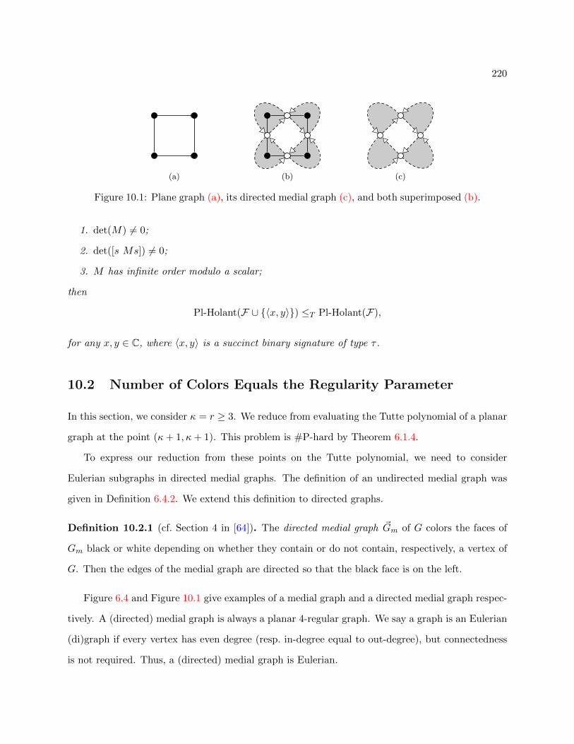
220

(a) (b) (c)

Figure 10.1: Plane graph (a), its directed medial graph (c), and both superimposed (b).

1. det(M) 6= 0;

2. det([s Ms]) 6= 0;

3. M has infinite order modulo a scalar;

then

Pl-Holant(F ∪ 〈x, y〉) ≤T Pl-Holant(F),

for any x, y ∈ C, where 〈x, y〉 is a succinct binary signature of type τ .

10.2 Number of Colors Equals the Regularity Parameter

In this section, we consider κ = r ≥ 3. We reduce from evaluating the Tutte polynomial of a planar

graph at the point (κ+ 1, κ+ 1). This problem is #P-hard by Theorem 6.1.4.

To express our reduction from these points on the Tutte polynomial, we need to consider

Eulerian subgraphs in directed medial graphs. The definition of an undirected medial graph was

given in Definition 6.4.2. We extend this definition to directed graphs.

Definition 10.2.1 (cf. Section 4 in [64]). The directed medial graph ~Gm of G colors the faces of

Gm black or white depending on whether they contain or do not contain, respectively, a vertex of

G. Then the edges of the medial graph are directed so that the black face is on the left.

Figure 6.4 and Figure 10.1 give examples of a medial graph and a directed medial graph respec-

tively. A (directed) medial graph is always a planar 4-regular graph. We say a graph is an Eulerian

(di)graph if every vertex has even degree (resp. in-degree equal to out-degree), but connectedness

is not required. Thus, a (directed) medial graph is Eulerian.

221

Building on previous work [105, 135, 63, 1], Ellis-Monaghan gave the following connection with

the diagonal of the Tutte polynomial. A monochromatic vertex is a vertex with all its incident

edges having the same color.

Lemma 10.2.2 (Equation (17) in [64]). Suppose G is a connected plane graph and ~Gm is its

directed medial graph. For κ ∈ N, let C(~Gm) be the set of all edge κ-labelings of ~Gm so that each

(possibly empty) set of monochromatic edges forms an Eulerian digraph. Then

κT(G;κ+ 1, κ+ 1) =∑

c ∈ C( ~Gm)

2m(c), (10.2.1)

where m(c) is the number of monochromatic vertices in the coloring c.

The Eulerian partitions in C(~Gm) have the property that the subgraphs induced by each par-

tition do not intersect (or crossover) each other due to the orientation of the edges in the medial

graph. We call the counting problem defined by the sum on the right-hand side of (10.2.1) counting

weighted Eulerian partitions over planar 4-regular graphs. This problem also has an expression as

a Holant problem using a succinct signature. To define this succinct signature, it helps to know

the following basic result about edge colorings.

When the number of available colors coincides with the regularity parameter of the graph, the

cuts in any coloring satisfy a well-known parity condition. This parity condition follows from a

more general parity argument (see (1.2) and the Parity Argument on page 95 in [117]). We state

this simpler parity condition and provide a short proof for completeness.

Lemma 10.2.3 (Parity Condition). Let G be a κ-regular graph and consider a cut C in G. For

any edge κ-coloring of G,

c1 ≡ c2 ≡ · · · ≡ cκ (mod 2),

where ci is the number of edges in C colored i for 1 ≤ i ≤ κ.

Proof. Consider two distinct colors i and j. Remove from G all edges not colored i or j. The

resulting graph is a disjoint union of cycles consisting of alternating colors i and j. Each cycle in

this graph must cross the cut C an even number of times. Therefore, ci ≡ cj (mod 2).

222

Consider all quaternary ADκ-gates on domain size κ ≥ 3. These gadgets have a succinct

signature of type τcolor = (P 1 11 1, P 1 2

1 2, P 1 2

2 1, P 1 1

2 2, P 1 4

2 3, P0), where

P 1 11 1

= (w, x, y, z) ∈ [κ]4 | w = x = y = z,

P 1 21 2

= (w, x, y, z) ∈ [κ]4 | w = x 6= y = z,

P 1 22 1

= (w, x, y, z) ∈ [κ]4 | w = y 6= x = z,

P 1 12 2

= (w, x, y, z) ∈ [κ]4 | w = z 6= x = y,

P 1 42 3

= (w, x, y, z) ∈ [κ]4 | w, x, y, z are distinct, and

P0 = [κ]4 − P 1 11 1− P 1 2

1 2− P 1 2

2 1− P 1 1

2 2− P 1 4

2 3.

Any quaternary signature of an ADκ-gate is constant on the first five parts of τcolor since ADκ is

domain invariant. Using Lemma 10.2.3, we can show that the entry corresponding to P0 is 0.

Lemma 10.2.4. Suppose κ ≥ 3 is the domain size and let F be a quaternary ADκ-gate with

succinct signature f of type τcolor. Then f(P0) = 0.

Proof. Let σ0 ∈ P0 be an edge κ-labeling of the external edges of F . Assume for a contradiction

that σ0 can be extended to an edge κ-coloring of F . We form a graph G from two copies of F

(namely, F1 and F2) by connecting their corresponding external edges. Then G has a coloring σ that

extends σ0. Consider the cut C = (F1, F2) in G whose cut set contains exactly those edges labeled

by σ0. By Lemma 10.2.3, the counts of the colors assigned by σ0 must satisfy the parity condition.

However, this is a contradiction since no edge κ-labeling in P0 satisfies the parity condition.

By Lemma 10.2.4, we denote a quaternary signature f of an ADκ-gate by the succinct signa-

ture 〈f(P 1 11 1

), f(P 1 21 2

), f(P 1 22 1

), f(P 1 12 2

), f(P 1 42 3

)〉 of type τcolor, which has the entry for P0 omitted.2

When κ = 3, P 1 42 3

is empty and we define its entry in the succinct signature to be 0.

2If κ > 4, then Lemma 10.2.3 further implies that these signatures are also 0 on P 1 42 3

. However, when κ = 4, this

value might be nonzero. The AD4 signature is an example of this. Instead of using this observation that depends onκ in our proof, we only construct gadgets such that their signatures are 0 on P 1 4

2 3for any value of κ.

223

Lemma 10.2.5. Let G be a connected plane graph and let Gm be the medial graph of G. Then

κT(G;κ+ 1, κ+ 1) = Pl-Holantκ(Gm; 〈2, 1, 0, 1, 0〉),

where the Holant problem has domain size κ and 〈2, 1, 0, 1, 0〉 is a succinct signature of type τcolor.

Proof. Let f = 〈2, 1, 0, 1, 0〉. By Lemma 10.2.2, we only need to prove that

∑c ∈ C( ~Gm)

2m(c) = Pl-Holantκ(Gm; f), (10.2.2)

where the notation is from Lemma 10.2.2.

Each c ∈ C(~Gm) is also an edge κ-labeling of Gm. At each vertex v ∈ V (~Gm), the four incident

edges are assigned at most two distinct colors by c. If all four edges are assigned the same color,

then the constraint f on v contributes a factor of 2 to the total weight. This is given by the

value in the first entry of f . Otherwise, there are two different colors, say x and y. Because the

orientation at v in ~Gm is cyclically “in, out, in, out”, the coloring around v can only be of the

form xxyy or xyyx. These correspond to the second and fourth entries of f . Therefore, every term

in the summation on the left-hand side of (10.2.2) appears (with the same nonzero weight) in the

summation Holantκ(Gm; f).

It is also easy to see that every nonzero term in Holantκ(Gm; f) appears in the sum on the

left-hand side of (10.2.2) with the same weight of 2 to the power of the number of monochromatic

vertices. In particular, any coloring with a vertex that is cyclically colored xyxy for different colors

x and y does not contribute because f(P 1 22 1

) = 0.

Remark. This result shows that this planar Holant problem is at least as hard as computing the

Tutte polynomial at the point (κ + 1, κ + 1) over planar graphs, which implies #P-hardness. Of

course they are equally difficult in the sense that both are #P-complete. In fact, they are more

directly related since every 4-regular plane graph is the medial graph of some plane graph.

By Theorem 6.1.4 and Lemma 10.2.5, the problem Pl-Holantκ(〈2, 1, 0, 1, 0〉) is #P-hard. We

state this as a corollary.

224

Figure 10.2: Quaternary gadget used in the interpolation construction below. Allvertices are assigned ADκ. The bold edge represents κ− 2 parallel edges.

Corollary 10.2.6. Suppose κ ≥ 3 is the domain size. Let 〈2, 1, 0, 1, 0〉 be a succinct quaternary

signature of type τcolor. Then Pl-Holantκ(〈2, 1, 0, 1, 0〉) is #P-hard.

With this connection established, we can now show that counting edge colorings is #P-hard

over planar regular graphs when the number of colors and the regularity parameter coincide.

Theorem 10.2.7. #κ-EdgeColoring is #P-hard over planar κ-regular graphs for all κ ≥ 3.

Proof. Let 〈2, 1, 0, 1, 0〉 be a succinct quaternary signature of type τcolor. We reduce from the prob-

lem Pl-Holantκ(〈2, 1, 0, 1, 0〉), which is #P-had by Corollary 10.2.6. We reduce to Pl-Holantκ(ADκ),

which expresses counting edge κ-colorings over planar κ-regular graphs as a Holant problem.

Consider the gadget in Figure 10.2, where the bold edge represents κ − 2 parallel edges. We

assign ADκ to both vertices. Up to a nonzero factor of (κ − 2)!, this gadget has the succinct

quaternary signature f = 〈0, 1, 1, 0, 0〉 of type τcolor. Now consider the recursive construction in

Figure 10.3. All vertices are assigned the signature f . Let fs be the succinct quaternary signature

N1 N2

Ns

Ns+1

Figure 10.3: Recursive construction to interpolate 〈2, 1, 0, 1, 0〉. The vertices are as-signed the signature of the gadget in Figure 10.2.

225

of type τcolor for the sth gadget of the recursive construction. Then f1 = f and fs = M sf0, where

M =

0 κ− 1 0 0 0

1 κ− 2 0 0 0

0 0 0 1 0

0 0 1 0 0

0 0 0 0 1

and f0 =

1

0

0

1

0

.

The signature f0 is simply the succinct quaternary signature of type τcolor for two parallel edges.

We can express M via the Jordan decomposition M = PΛP−1, where

P =

1 1− κ 0 0 0

1 1 0 0 0

0 0 1 1 0

0 0 1 −1 0

0 0 0 0 1

and Λ = diag(κ− 1,−1, 1,−1, 1). Then for t = 2s, we have

ft = P

κ− 1 0 0 0 0

0 −1 0 0 0

0 0 1 0 0

0 0 0 −1 0

0 0 0 0 1

t

P−1

1

0

0

1

0

= P

x 0 0 0 0

0 1 0 0 0

0 0 1 0 0

0 0 0 1 0

0 0 0 0 1

P−1

1

0

0

1

0

=

y + 1

y

0

1

0

,

where x = (κ− 1)t and y = x−1κ .

Consider an instance Ω of Pl-Holantκ(〈2, 1, 0, 1, 0〉). Suppose 〈2, 1, 0, 1, 0〉 appears n times in Ω.

We construct from Ω a sequence of instances Ωt of Pl-Holantκ(f) indexed by t, where t = 2s with

s ≥ 0. We obtain Ωt from Ω by replacing each occurrence of 〈2, 1, 0, 1, 0〉 with the gadget ft.

As a polynomial in x = (κ− 1)t, Pl-Holantκ(Ωt; f) is independent of t and has degree at most

n with integer coefficients. Using our oracle for Pl-Holantκ(f), we can evaluate this polynomial

226

at n + 1 distinct points x = (κ − 1)2s for 0 ≤ s ≤ n. Then via polynomial interpolation, we can

recover the coefficients of this polynomial efficiently. Evaluating this polynomial at x = κ + 1 (so

that y = 1) gives the value of Pl-Holantκ(Ω; 〈2, 1, 0, 1, 0〉), as desired.

Remark. For κ = 3, the interpolation step is actually unnecessary since the succinct signature of

f2 happens to be 〈2, 1, 0, 1, 0〉.

When κ = 3, it is easy to extend Theorem 10.2.7 by further restricting to simple graphs.

Theorem 10.2.8. #3-EdgeColoring is #P-hard over simple planar 3-regular graphs.

Proof. By Theorem 10.2.7, it suffices to efficiently compute the number of edge 3-colorings of a

planar 3-regular graph G that might have self-loops and parallel edges. Furthermore, we can

assume that G is connected since the number of edge colorings is multiplicative over connected

components. If G contains a self-loop, then there are no edge colorings in G, so assume G contains

no self-loops. If G also contains no parallel edges, then G is simple and we are done.

Thus, assume that G contains n vertices and parallel edges between some distinct vertices u

and v. If u and v are connected by three edges, then this constitutes the whole graph, which has

six edge 3-colorings. Otherwise, u and v are connected by two edges. Then there exist vertices u′

and v′ such that u and u′ are connected by a single edge, v and v′ are connected by a single edge,

and u′ 6= v′. In any edge 3-coloring of G, it is easy to see that the edges (u, u′) and (v, v′) must be

assigned the same color. By removing u, v, and their incident edges while adding an edge between

u′ and v′, we have a planar 3-regular graph G′ on n− 2 vertices with half as many edge colorings

as G. Then by induction, we can efficiently compute the number of edge 3-colorings in G′.

Section 11.4, we give an alternative proof of Theorem 10.2.7, which uses the interpolation

techniques we develop in Section 11.3. The purpose of Section 11.4 is to show how a recursive

construction in an interpolation proof can be used to form a hypothesis about possible invariance

properties. One example of an invariance property is that any planar ADκ-gate with a succinct

quaternary signature 〈a, b, c, d, e〉 of type τcolor must satisfy a+ c = b+ d (Lemma 11.4.1).

227

f1 f2

f`

f`+1

Figure 10.4: Recursive construction to interpolate any succinct binary signature of typeτ2. All vertices are assigned the same succinct binary signature of type τ2.

10.3 Number of Colors Exceeds the Regularity Parameter

Now we consider κ > r ≥ 3. we reduce from the problem of counting vertex κ-colorings over

planar graphs. This problem is also #P-hard by the same dichotomy for the Tutte polynomial

(Theorem 6.1.4) since the chromatic polynomial is a specialization the Tutte polynomial.

Proposition 10.3.1 (Proposition 6.3.1 in [12]). Let G = (V,E) be a graph. Then χ(G;λ), the

chromatic polynomial of G, is expressed as a specialization of the Tutte polynomial via the relation

χ(G;λ) = (−1)|V |−k(G)λk(G) T(G; 1− λ, 0),

where k(G) is the number of connected components of the graph G.

The first step in the proof is to interpolate every possible binary signature that is domain

invariant, which are necessarily symmetric. These signatures have the succinct signature type τ2.

Lemma 10.3.2. Suppose κ ≥ 3 is the domain size and let x, y ∈ C. If we assign the succinct

binary signature 〈x, y〉 of type τ2 to every vertex of the recursive construction in Figure 10.4, then

the corresponding recurrence matrix is[x (κ−1)yy x+(κ−2)y

]with eigenvalues x+ (κ− 1)y and x− y.

Proof. Let f` be the signature of the `th gadget in this construction. To obtain f`+1 from f`,

we view f` as a column vector and multiply it by the recurrence matrix M =[x (κ−1)yy x+(κ−2)y

]. In

general, we have f` = M `f0, where f0 is the initial signature, which is just a single edge and has

the succinct binary signature 〈1, 0〉 of type τ2. The (column) eigenvectors of M are [ 11 ] and

[1−κ

1

]with eigenvalues x+ (κ− 1)y and x− y respectively, as claimed.

Consider the recursive construction in Figure 10.4. To every vertex, we assign the succinct

binary signature 〈x, y〉. Since the initial signature is s = 〈1, 0〉, the determinant of the matrix

228

Figure 10.5: Binary gadget used in the interpolation construction of Figure 10.4. Bothvertices are assigned ADr and the bold edge represents r − 1 parallel edges.

[s Ms] is simply y. In order to interpolate all binary succinct signatures of type τ2, we need to

satisfy the second condition of Lemma 10.1.3, which is y 6= 0. However when y = 0, the recurrence

matrix is a scalar multiple of the identity matrix, which implies that the eigenvalues are the same.

For two dimensional interpolation using a matrix with a full basis of eigenvectors, as is the case here,

the third condition of Lemma 10.1.3 is equivalent to the ratio of the eigenvalues not being a root

of unity. In particular, the eigenvalues cannot be the same. Therefore, when using the recursive

construction in Figure 10.4, it suffices to satisfy the first and third conditions of Lemma 10.1.3. We

state this as a corollary.

Corollary 10.3.3. Suppose F is a set of signatures. Let s = 〈1, 0〉 of type τ2 be the initial succinct

binary signature and let M ∈ C2×2 be the recurrence matrix for some infinite sequence of planar

F-gates defined by the recursive construction in Figure 10.4. If M satisfies the following conditions,

1. det(M) 6= 0;

2. M has infinite order modulo a scalar;

then

Pl-Holantκ(F ∪ 〈x, y〉) ≤T Pl-Holantκ(F),

for any x, y ∈ C, where 〈x, y〉 is a succinct binary signature of type τ2.

Lemma 10.3.4. Suppose κ is the domain size with κ > r for any integer r ≥ 3, and x, y ∈ C. Let

F be a signature set containing ADr. Then

Pl-Holantκ(F ∪ 〈x, y〉) ≤T Pl-Holantκ(F),

where 〈x, y〉 is a succinct binary signature of type τ2.

Proof. Let (n)k = n(n − 1) · · · (n − k + 1) be the kth falling power of n. Consider the gadget in

Figure 10.5. We assign ADr to both vertices. The succinct binary signature of type τ2 for this

229

gadget is f = 〈(κ− 1)r−1, (κ− 2)r−1〉. Up to a nonzero factor of (κ− 2)r−2, we have the signature

f ′ = 1(κ−2)r−2

f = 〈κ− 1, κ− r〉.

Consider the recursive construction in Figure 10.4. We assign f ′ to all vertices. Then by

Lemma 10.3.2, the two eigenvalues of the corresponding recurrence matrix are (r − 1) > 0 and

(κ− 1)(κ− r + 1) > 0. Thus, M is nonsingular. Furthermore, the eigenvalues are not equal since

κ 6∈ 0, r. Therefore, we are done by Corollary 10.3.3.

Next we show that Pl-Holantκ(ADr) is at least as hard as Pl-Holantκ(AD3). To overcome a

difficulty when r is even, we use the the concept of a planar pairing, which was introduced in

Section 6.3.

Lemma 10.3.5. Suppose κ is the domain size with κ > r for any integer r ≥ 3. Then

Pl-Holantκ(AD3) ≤T Pl-Holantκ(ADr).

Proof. By Lemma 10.3.4, we can assume that 〈1, 1〉 is available. Take ADr and first form t =⌈r−4

2

⌉self-loops. Then add a new vertex on each self-loop and assign 〈1, 1〉 to each of these new vertices.

Up to a nonzero factor of (κ− 3)2t, the resulting signature is AD3 if r is odd and AD4 if r is even.

To reduce from r = 3 to r = 4, we use a planar pairing, which can be efficiently computed by

Lemma 6.3.4. We add a new vertex on each edge in a planar pairing and assign 〈1, 1〉 to each of

these new vertices. Then up to a nonzero factor of κ− 3, the signature at each vertex of the initial

graph is effectively AD3.

The succinct binary signature 〈1−κ, 1〉 of type τ2 has a special property. Let u be any constant

unary signature, which has a succinct signature of type τ1. If 〈1− κ, 1〉 is connected to u, then the

resulting unary signature is identically zero.

This observation is the key to what follows. We use it in the next lemma to achieve what would

appear to be an impossible task. The requirements, if duly specified, would result in multiple

conditions to be satisfied by nine separate polynomials pertaining to some construction in place

of the gadget in Figure 10.6. And yet we are able to use just one degree of freedom to cause

seven of the polynomials to vanish, satisfying most of these conditions. In addition, the other two

230

Figure 10.6: The Bobby Fischer gadget, which achieves many objectives using only asingle degree of freedom.

polynomials are not forgotten. They are nonzero and their ratio is not a root of unity, which allows

interpolation to succeed.

This ability to satisfy a multitude of constraints simultaneously in one magic stroke reminds us

of some unfathomably brilliant moves by Bobby Fischer, the chess genius extraordinaire, and so we

name this gadget (Figure 10.6) the Bobby Fischer gadget.

This gadget is the new idea that allows us to prove Theorem 10.3.8.

Lemma 10.3.6. Suppose κ ≥ 3 is the domain size and a, b ∈ C. Let F be a signature set containing

the succinct ternary signature 〈a, b, b〉 of type τ3 and the succinct binary signature 〈1−κ, 1〉 of type

τ2. If a 6= b, then

Pl-Holantκ(F ∪ =4) ≤T Pl-Holantκ(F).

Proof. Consider the gadget in Figure 10.6. We assign 〈a, b, b〉 to the circle vertices and 〈1−κ, 1〉 to

the square vertex. This gadget has a succinct quaternary signature of type τ4, which has length 9.

However, all but two of the entries in this succinct signature must be 0.

To see this, consider an assignment that assigns different values to the two edges incident to

the circle vertex on top. Since the assignment to these two edges differ, the signature 〈a, b, b〉

contributes a factor of b regardless of the value of its third edge, which is connected to the square

vertex assigned 〈1−κ, 1〉. From the perspective of 〈1−κ, 1〉, this behavior is equivalent to connecting

it to the succinct unary signature b〈1〉 of type τ1. Thus, the sum over the possible assignments to

this third edge is 0. The same argument shows that the two edges incident to the circle vertex on

the bottom do not contribute anything to the Holant sum when assigned different values.

Thus, any nonzero contribution to the Holant sum comes from assignments where the top two

dangling edges are assigned the same value and the bottom two dangling edges are assigned the

231

same value. There are only two entries that satisfy this requirement in the succinct quaternary

signature of type τ4 for this gadget, which are the entries for P 1 11 1

and P 1 12 2

. To compute those

two entries, we use the following trick. Since the two external edges of each circle vertex must

be assigned the same value, we think of them as just a single edge. Then the effective succinct

binary signature of type τ2 for the circle vertices is just 〈a, b〉. By connecting the first 〈a, b〉 with

〈1−κ, 1〉, the result is (a−b)〈1−κ, 1〉 like it is an eigenvector. Connecting the other copy of 〈a, b〉 to

(a−b)〈1−κ, 1〉 gives (a−b)2〈1−κ, 1〉. This computation is expressed via the matrix multiplication

[bJκ + (a− b)Iκ][Jκ− κIκ][bJκ + (a− b)Iκ] = (a− b)[Jκ− κIκ][bJκ + (a− b)Iκ] = (a− b)2[Jκ− κIκ].

Thus up to a nonzero factor of (a − b)2, the corresponding succinct quaternary signature of type

τ4 for this gadget is f = 〈1− κ, 0, 0, 0, 0, 0, 1, 0, 0〉.

Consider the recursive construction in Figure 10.3. We assign f to all vertices. Let fs be

the signature of the sth gadget in this construction. The seven entries that are 0 in the succinct

signature of type τ4 for f are also 0 in the succinct signature of type τ4 for fs. Thus, we can express

fs via a succinct signature of type τ ′4 with length 2, defined as follows. The first two parts in τ ′4

are P 1 11 1

and P 1 12 2

from the succinct signature type τ4. The last part contains all the remaining

assignments. Then the succinct signature for fs of type τ ′4 is M sf0, where M =[

1−κ 00 1

]and

f0 = 〈1, 1〉, which is just the succinct signature of type τ ′4 for two parallel edges.

Clearly the conditions in Lemma 10.1.3 hold, so we can interpolate any succinct signature of

type τ ′4. In particular, we can interpolate our target signature =4, which is 〈1, 0〉 when expressed

as a succinct signature of type τ ′4.

Remark. The nine polynomials mentioned before Lemma 10.3.6 correspond to the nine entries of

some quaternary gadget with a succinct signature of type τ4. In light of Lemma 10.3.4, this gadget

might involve many succinct binary signatures 〈x, y〉 of type τ2 for various choices of x, y ∈ C.

Each distinct binary signature provides an additional degree of freedom to these polynomials. Our

construction in Figure 10.6 only requires one binary signature 〈x, y〉 and we use our one degree of

freedom to set xy = 1− κ.

With the aid of the succinct unary signature 〈1〉 of type τ1 and the succinct binary signature

〈0, 1〉 of type τ2, the assumptions in the previous lemma are sufficient to prove #P-hardness.

232

Figure 10.7: Local holographic transformation gadget construction for a ternary signa-ture.

Corollary 10.3.7. Suppose κ ≥ 3 is the domain size and a, b ∈ C. Let F be a signature set

containing the succinct ternary signature 〈a, b, b〉 of type τ3, the succinct unary signature 〈1〉 of type

τ1, and the succinct binary signatures 〈1− κ, 1〉 and 〈0, 1〉 of type τ2. If a 6= b, then Pl-Holantκ(F)

is #P-hard.

Proof. By Lemma 10.3.6, we have =4. Connecting 〈1〉 to =4 gives =3. With =3, we can construct

the equality signatures of every arity. Along with the binary disequality signature 6=2, which is the

succinct binary signature 〈0, 1〉 of type τ2, we can express the problem of counting the number of

vertex κ-colorings over planar graphs. By Proposition 10.3.1, this is, up to a nonzero factor, the

problem of evaluating the Tutte polynomial at (1− κ, 0), which is #P-hard by Theorem 6.1.4.

Now we can show that counting edge colorings is #P-hard over planar regular graphs when

there are more colors than the regularity parameter.

Theorem 10.3.8. #κ-EdgeColoring is #P-hard over planar r-regular graphs for all κ > r ≥ 3.

Proof. By Lemma 10.3.5, it suffices to consider r = 3. By Lemma 10.3.4, we can assume that any

succinct binary signature of type τ2 is available.

Consider the gadget in Figure 10.7. We assign AD3 to the circle vertex and 〈3 − κ, 1〉 to

the square vertices. By Lemma 9.2.6, the succinct ternary signature of type τ3 for this gadget is

f = 2(κ− 2)〈−(κ− 3)(κ− 1), 1, 1〉.

Now take two edges of AD3 and connect them to the two edges of 〈1, 1〉. Up to a nonzero factor

of (κ− 1)(κ− 2), this gadget has the succinct unary signature 〈1〉 of type τ1. Then we are done by

Corollary 10.3.7.

233

10.4 Closing Thoughts

Genesis I think the story about how this work began is fascinating. Let me share it with you.

After publishing [73] in December 2012, I was using my free time to work on a draft Wikipedia

page about Holant that I had created the previous December. While adding example problems, I

came to the section about graph colorings. Edge coloring is the most natural higher domain Holant

problem, and I quickly added it. For each example, I would also add a reference that studied the

problem and determined its counting complexity. But for this problem, I was at a loss. None of

the papers that I knew about or could find had done this. I emailed Jin-Yi Cai on the last day of

the year, and we began an informal discussion about the problem.

January of 2013 was a month that I had been looking forward to for some time. From the 13th

to the 18th, Heng Guo and I were going to attend Dagstuhl Seminar 13031 about Computational

Counting. We arrived a few days early and visited Mingji Xia at the Max Planck Institute for

Informatics. We discussed the problem of edge coloring and came up with some ideas. With help

from Jin-Yi Cai over email, we had (on January 14th) a sketch of a proof that counting edge κ-

colorings was #P-hard over planar κ-regular graphs for κ ≥ 3. While at the seminar, we didn’t

have the time to check all the details.

In the meantime, no less than three people approached me and asked if I knew the complexity

of counting edge colorings. I was stunned. Normally I wouldn’t share a result that I wasn’t sure

about, but I made an exception for this special event. When we returned home, we realized that

planarity imposes a restriction that did not arise in our proof sketch.3 With this restriction, we did

not know of any #P-hard problem from which to reduce. Fortunately, we found such a problem.

The coincidence is that it came from other conversations at Dagstuhl.

I presented [73] near the beginning of the seminar. One of the highlights of this work (presented

here in Section 6.4) is a reduction from evaluating the Tutte polynomial of a planar graph at the

point (3, 3), a result by Las Vergnas [136]. One of the people at the seminar was Joanna Ellis-

Monaghan. After my talk, she told me that she had generalized the result of Las Vergnas to any

positive integer point on the diagonal [64]. We spent many hours together discussing this result

3The restriction imposed by planarity is the one given in Lemma 11.4.1.

234

and many other things, but when I left the seminar, I had still not internalized her generalization.

When I returned home, I began working in parallel. On the one hand, we determined that we

could interpolate anything that satisfied a certain equation (cf. Section 11.4). On the other hand,

I was emailing Joanna Ellis-Monaghan to help clarify my understanding of her generalization. I

realized (on February 7th) that her generalization corresponded to a Holant problem that satisfied

the same equation!

I typically think of Holant problems being so expressive and techniques like polynomial inter-

polation being so strong that there are many problems one can reduce from in order to prove new

hardness results. This is not one of those cases. I know of no other way to show that count-

ing edge κ-colorings is #P-hard over planar κ-regular graphs for κ ≥ 3 except by using Joanna

Ellis-Monaghan’s work.

Another remark about the Bobby Fischer gadget The way we presented the Bobby Fischer

gadget is not exactly how we found it. We make it look as though we used one degree of freedom to

satisfy seven conditions (that is, setting seven signature entries to 0), but I think it is more accurate

to say that we use two degrees of freedom to satisfy eight conditions. The eighth condition is implicit

in Lemma 10.3.6. It is that we have a succinct ternary signature 〈a, b, c〉 of type τ3 with b = c.

This assumption is satisfied in the proof of Theorem 10.3.8 via a local holographic transformation,

which uses one degree of freedom.

The “original Bobby Fischer gadget” was two copies of the same ternary local-holographic-

transformation gadget (one degree of freedom) with one edge from each connected together through

an arbitrary succinct binary signature of type τ2 (a second degree of freedom). Then we looked for

any interesting choices of those two parameters. At this point, it is rather obvious to consider the

parameter choices that we did. What remains is to realize that the resulting signature can be used

to interpolate =4 and that =4 quickly leads to a reduction from counting vertex colorings.

The way we presented it is our attempt to be conceptual as possible. We presented it as though

one might have had the foresight to select these parameter choices from the beginning.

235

Chapter 11

Dichotomy for Higher Domain Holant

Problems over Planar 3-Regular

Graphs

We adapt and extend our proof techniques from the previous chapter to obtain a dichotomy for

Pl-Holantκ(f), where f is a succinct ternary signature of type τ3 on domain size κ ≥ 3 with complex

weights. A special case of this result is that counting edge κ-colorings is #P-hard over planar 3-

regular graphs for all κ ≥ 3. A key ingredient in the proof includes an effective version of Siegel’s

Theorem on finiteness of integer solutions for a specific algebraic curve. We use this to show that

a specific polynomial p(x, y) has an explicitly listed finite set of integer solutions. We also apply

some elementary Galois theory and determine the Galois groups of some specific polynomials. This

work was published in [32, 33].

11.1 Background

What do Siegel’s Theorem and Galois theory have to do with complexity theory? In this chapter,

we show that an effective version of Siegel’s Theorem on finiteness of integer solutions for a specific

algebraic curve and an application of elementary Galois theory are key ingredients in a chain of

236

steps that lead to a complexity classification of some counting problems. More specifically, we

consider a certain class of counting problems that are expressible as Holant problems with an

arbitrary domain of size κ over 3-regular graphs, and prove a dichotomy theorem for this class of

problems. The hardness, and thus the dichotomy, holds even when restricted to planar graphs.

Among other things, the proof of the dichotomy theorem depends on the following: (A) the specific

polynomial p(x, y) = x5 − 2x3y − x2y2 − x3 + xy2 + y3 − 2x2 − xy has only the integer solutions

(x, y) = (−1, 1), (0, 0), (1,−1), (1, 2), (3, 3), and (B) the determination of the Galois groups of some

specific polynomials.

The techniques we developed to prove Theorem 10.1.1 naturally extend to Holant problems

defined by any succinct ternary signature of type τ3. We prove a dichotomy theorem for such

functions with complex weights.

Theorem 11.1.1. Suppose κ ≥ 3 is the domain size and a, b, c ∈ C. Then either Holantκ(〈a, b, c〉)

is computable in polynomial time or Pl-Holantκ(〈a, b, c〉) is #P-hard. Furthermore, given a, b, c,

there is a polynomial-time algorithm that decides which is the case.

See Theorem 11.8.1 for an explicit listing of the tractable cases. Counting edge κ-colorings over

3-regular graphs is the special case when 〈a, b, c〉 = 〈0, 0, 1〉.

There is only one previous dichotomy theorem for higher domain Holant problems [51]. It is

a dichotomy for a single symmetric ternary signature on domain size κ = 3 in the framework of

Holant∗ problems, which means that all unary signatures are assumed to be freely available. An

important difference is that Theorem 11.1.1 is for general domain size κ ≥ 3 while the previous

result is for domain size κ = 3. Dichotomy theorems for an arbitrary domain size are generally

difficult to prove. The Feder-Vardi Conjecture for decision Constraint Satisfaction Problems (CSP)

is still open [67]. It was a major achievement to prove this conjecture for domain size 3 [15]. The

#CSP dichotomy was proved after a long series of work [17, 16, 14, 58, 13, 53, 22, 35, 60, 71, 36, 20].

In Theorem 11.1.2, the notation f_g denotes the signature that results from connecting one

edge incident to a vertex assigned the signature f to one edge incident to a vertex assigned the

signature g. When f and g are both unary signatures, which are represented by vectors, then the

resulting 0-ary signature is just a scalar.

237

Theorem 11.1.2 (Theorem 3.1 in [51]). Let f be a symmetric ternary signature on domain size 3.

Then Holant∗3(f) is #P-hard unless f is of one of the following forms, in which case, the problem

is computable in polynomial time.

1. There exists α, β, γ ∈ C3 that are mutually orthogonal (i.e. α_β = α_γ = β_γ = 0) and

f = α⊗3 + β⊗3 + γ⊗3;

2. There exists α, β1, β2 ∈ C3 such that α_β1 = α_β2 = β_1 β1 = β_2 β2 = 0 and

f = α⊗3 + β⊗31 + β⊗3

2 ;

3. There exists β, γ ∈ C3 and fβ ∈ (C3)⊗3 such that β 6= 0, β_β = 0, f_β β = 0, and

f = fβ + β⊗2 ⊗ γ + β ⊗ γ ⊗ β + γ ⊗ β⊗2.

Some domain invariant signatures are tractable by Theorem 11.1.2.

Corollary 11.1.3. Suppose the domain size is 3 and a, b, λ ∈ C. Let f be a succinct ternary

signature of type τ3. Then Holant(f) is computable in polynomial time when f has one of the

following forms:

1. f = λ〈1, 0, 0〉 = λ[(1, 0, 0)⊗3 + (0, 1, 0)⊗3 + (0, 0, 1)⊗3

];

2. f = 3λ〈−5,−2, 4〉 = λ[(1,−2,−2)⊗3 + (−2, 1,−2)⊗3 + (−2,−2, 1)⊗3

];

3. f = 〈a, b, a〉 = a+2b3 (1, 1, 1)⊗3 + a−b

3

[(1, ω, ω2)⊗3 + (1, ω2, ω)⊗3

],

where ω is a primitive third root of unity.

In Corollary 11.1.3, form 1 is the ternary equality signature =3, which is trivially tractable for

any domain size. Then form 2 is just form 1 after a holographic transformation by the matrix

T =[ 1 −2 −2−2 1 −2−2 −2 1

], which is orthogonal after scaling by 1

3 . This is an example of two problems that

must have the same complexity by Lemma 3.2.2.

The tractability of these two problems for higher domain sizes is stated in the following corollary.

238

Corollary 11.1.4. Suppose κ ≥ 3 is the domain size and λ ∈ C. Let f be a succinct ternary

signature of type τ3. Then Holant(f) is computable in polynomial time if f has one of the following

forms:

1. f = λ〈1, 0, 0〉;

2. f = λT⊗3〈1, 0, 0〉 = λκ〈κ2 − 6κ+ 4,−2(κ− 2), 4〉,

where T = κIκ − 2Jκ.

Note that T = κIκ − 2Jκ is an orthogonal matrix after scaling by 1κ .

The two cases in Corollary 11.1.4 are respectively product type and transformable to product

type. There are also two affine tractable cases that appear in our dichotomy. We already discussed

them in Section 4.2. We restate the first using our succinct signature notation.

Corollary 11.1.5 (Restatement of Corollary 4.2.11). Suppose the domain size is 3 and suppose

a, c ∈ C. Let T ∈ O3(C) and let 〈a, 0, c〉 be a succinct ternary signature of type τ3. If a3 = c3, then

Holant3(T⊗3〈a, 0, c〉) is computable in polynomial time.

The second result requires some additional proof.

Lemma 11.1.6. Suppose the domain size is 4 and λ, µ ∈ C. Let 〈µ2, 1, µ〉 be a succinct ternary

signature of type τ3. If µ = −1 + ε2i with ε = ±1, then Holant(λ〈µ2, 1, µ〉) is computable in

polynomial time.

Proof. Let T = 12

[ x y y yy x y yy y x yy y y x

], where x = −3− εi and y = 1− εi. Then up to a factor of λn on graphs

with n vertices, the output of Holant(λ〈µ2, 1, µ〉) is the same as the output for

Holant(〈µ2, 1, µ〉) = Holant(〈−3− ε4i, 1,−1 + ε2i〉)

≡T Holant(=2 | T⊗3(=3))

≡ Holant((=2)T⊗2 | =3)

≡ Holant(2〈1,−1〉 | =3).

After removing the factor of 2 from the signature on the left, we are done by Lemma 4.2.14.

239

We restate this lemma as a simple corollary for later convenience.

Corollary 11.1.7. Suppose the domain size is 4 and a, b, c ∈ C. Let 〈a, b, c〉 be a succinct ternary

signature of type τ3. If a+ 5b+ 2c = 0 and 5b2 + 2bc+ c2 = 0, then Holant(〈a, b, c〉) is computable

in polynomial time.

Proof. Since a = −5b− 2c and b = 15(−1± 2i)c, after scaling by µ = −1∓ 2i, we have µ〈a, b, c〉 =

c〈µ2, 1, µ〉 and are done by Lemma 11.1.6.

11.2 Proof Outline and Techniques

As usual, the difficult part of a dichotomy theorem is to carve out exactly the tractable prob-

lems in the class, and prove all the rest #P-hard. A dichotomy theorem for Holant problems

has the additional difficulty that some tractable problems are only known to be tractable via a

holographic reduction, which can make the appearance of the problem rather unexpected. The

problem Holant4(〈−3−4i, 1,−1+2i〉) that we just discussed is of this type. In order to understand

all problems in a Holant problem class, we must deal with such problems. Dichotomy theorems for

graph homomorphisms and for #CSP do not have to deal with as varied a class of such problems,

since they implicitly assume all Equality signatures are available and must be preserved. This

restricts the possible transformations.

Our #P-hardness results are obtained by reducing from evaluations of the Tutte polynomial

over planar graphs. A dichotomy is known for such problems (Theorem 6.1.4).

The chromatic polynomial, a specialization of the Tutte polynomial (Proposition 10.3.1), is

concerned with vertex colorings. On domain size κ, one starting point of our hardness proofs is

the chromatic polynomial, which contains the problem of counting vertex colorings using at most

κ colors. By the planar dichotomy for the Tutte polynomial, this problem is #P-hard for all κ ≥ 3.

Another starting point for our hardness reductions is the evaluation of the Tutte polynomial at

an integer diagonal point (x, x), which is #P-hard for all x ≥ 3 by the same planar Tutte dichotomy.

These are new starting places for reductions involving Holant problems. These problems were known

to have a so-called state-sum expression (Lemma 10.2.2), which is a sum over weighted Eulerian

240

partitions. This sum is not over the original planar graph but over its directed medial graph,

which is always a planar 4-regular graph (Figure 6.4 and Figure 10.1). We show that this state-

sum expression is naturally expressed as a Holant problem with a particular quaternary signature

(Lemma 10.2.5).

To reduce from these two problems, we execute the following strategy. First, we attempt to

construct the succinct unary signature 〈1〉 of type τ1. (Lemma 11.5.1). Second, we attempt to

interpolate all succinct binary signatures assuming that we have 〈1〉 (Section 11.6). Lastly, we

attempt to construct a succinct ternary signature 〈a, b, c〉 of type τ3 with the special property b = c

assuming that all these binary signatures are available (Lemma 11.7.1). At each step, there are

some problems specified by 〈a, b, c〉 for which our attempts fail. In such cases, we directly obtain a

dichotomy without the help of additional signatures. See Figure 11.1 for a flow chart of hardness

reductions.

Below we highlight some of our proof techniques.

Interpolation within an orthogonal subspace We develop the ability to interpolate when

faced with some nontrivial null spaces inherently present in interpolation constructions. In any

construction involving an initial signature and a recurrence matrix, it is possible that the initial

signature is orthogonal to some row eigenvectors of the recurrence matrix. Previous interpolation

results always attempt to find a construction that avoids this. In the present chapter, this avoidance

seems impossible. In Section 11.3, we prove an interpolation result that can succeed in this situation

to the greatest extent possible. We prove that one can interpolate any signature provided that it

is orthogonal to the same set of row eigenvectors, and the relevant eigenvalues satisfy a lattice

condition (Lemma 11.3.6).

Satisfy lattice condition via Galois theory A key requirement for this interpolation to suc-

ceed is the lattice condition (Definition 11.3.3), which involves the roots of the characteristic poly-

nomial of the recurrence matrix. We use Galois theory to prove that our constructions satisfy this

condition. If a polynomial has a large Galois group, such as Sn or An, and its roots do not all have

the same complex norm, then we show that its roots satisfy the lattice condition (Lemma 11.3.5).

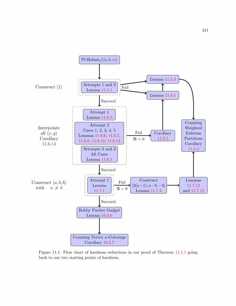
241

Pl-Holantκ(〈a, b, c〉)

Attempts 1 and 2Lemma 11.5.1

Attempt 1Lemma 11.6.5

Attempt 2Cases 1, 2, 3, 4, 5

Lemmas 11.6.6, 11.6.7,11.6.8, 11.6.12, 11.6.13

Attempts 3 and 4All Cases

Lemma 11.6.1

Attempt 1Lemma11.7.1

Bobby Fischer GadgetLemma 10.3.6

Counting Vertex κ-ColoringsCorollary 10.3.7

Fail

Interpolateall 〈x, y〉Corollary11.6.14

Construct 〈1〉

Construct 〈a, b, b〉with a 6= b

Corollary11.5.5

Lemma 11.5.3

Lemma 11.5.4

Construct〈3(κ−1), κ−3,−3〉

Lemma 11.7.3

CountingWeightedEulerian

PartitionsCorollary

11.5.2

Lemmas11.7.12

and 11.7.13

Succeed

Succeed

Succeed

Fail

B = 0

Fail

A = 0

Figure 11.1: Flow chart of hardness reductions in our proof of Theorem 11.1.1 goingback to our two starting points of hardness.

242

Effective Siegel’s Theorem via Puiseux series We need to determine the Galois groups for

an infinite family of polynomials, one for each domain size. If these polynomials are irreducible,

then we can show they all have the full symmetric group as their Galois group, and hence fulfill the

lattice condition. We suspect that these polynomials are all irreducible but are unable to prove it.

A necessary condition for irreducibility is the absence of any linear factor. This infinite family

of polynomials, as a single bivariate polynomial in (x, κ), defines an algebraic curve, which has

genus 3. By a well-known theorem of Siegel [115], there are only a finite number of integer values

of κ for which the corresponding polynomial has a linear factor. However this theorem and others

like it are not effective in general. There are some effective versions of Siegel’s Theorem that can be

applied to the algebraic curve, but the best general effective bound is over 1020,000 [140] and hence

cannot be checked in practice. Instead, we use Puiseux series to show that this algebraic curve has

exactly five explicitly listed integer solutions (Lemma 11.7.6).

Eigenvalue Shifted Triples For a pair of eigenvalues, the lattice condition is equivalent to the

statement that the ratio of these eigenvalues is not a root of unity. A sufficient condition is that the

eigenvalues have distinct complex norms. We prove three results, each of which is a different way

to satisfy this sufficient condition. Chief among them is the technique we call an Eigenvalue Shifted

Triple (EST). These generalize the technique of Eigenvalue Shifted Pairs from [93]. In an EST,

we have three recurrence matrices, each of which differs from the other two by a nonzero additive

multiple of the identity matrix. Provided these two multiples are linearly independent over R, we

show at least one of these matrices has eigenvalues with distinct complex norms (Lemma 11.6.11).

(However determining which one succeeds is a difficult task; but we need not know that).

E Pluribus Unum When the ratio of a pair of eigenvalues is a root of unity, it is a challenge

to effectively use this failure condition. Direct application of this cyclotomic condition is often of

limited use. We introduce an approach that uses this cyclotomic condition effectively. A direct

recursive construction involving these two eigenvalues only creates a finite number of different

signatures. We reuse all of these signatures in a multitude of new interpolation constructions

(Lemma 11.6.4), one of which we hope will succeed. If the eigenvalues in all of these constructions

243

also satisfy a cyclotomic condition, then we obtain a more useful condition than any of the previous

cyclotomic conditions. This idea generalizes the anti-gadget technique from Chapter 5, which only

reuses the “last” of these signatures.

Local holographic transformation One reason to obtain all succinct binary signatures is for

use in the gadget construction known as a local holographic transformation (Figure 11.8). This

construction mimics the effect of a holographic transformation applied on a single signature. In

particular, using this construction, we attempt to obtain a succinct ternary signature of the form

〈a, b, b〉, where a 6= b (Lemma 11.7.1). This signature turns out to have some magical properties in

the Bobby Fischer gadget, which we discuss next.

Bobby Fischer gadget Typically, any combinatorial construction for higher domain Holant

problems produces very intimidating looking expressions that are nearly impossible to analyze. In

our case, it seems necessary to consider a construction that has to satisfy multiple requirements

involving at least nine polynomials. However, we are able to combine the signature 〈a, b, b〉, where

a 6= b, with a succinct binary signature of our choice in a special construction that we call the

Bobby Fischer gadget (Figure 10.6). This gadget is able to satisfy seven conditions using just one

degree of freedom (Lemma 10.3.6). This ability to satisfy a multitude of constraints simultaneously

in one magic stroke reminds us of some unfathomably brilliant moves by Bobby Fischer, the chess

genius extraordinaire. We first encountered the Bobby Fischer gadget in the previous chapter in

Section 10.3, but it is a crucial ingredient in the current chapter as well.

11.3 An Interpolation Result

The goal of this section is to generalize an interpolation result from [50], which we rephrase using

our notion of a succinct signature (cf. Lemma 10.1.3).

Theorem 11.3.1 (Theorem 3.5 in [50]). Suppose F is a set of signatures over a domain of size κ

and τ is a succinct signature type with length 3. If there exists an infinite sequence of planar F-

gates defined by an initial succinct signature s ∈ C3×1 of type τ and a recurrence matrix M ∈ C3×3

244

with eigenvalues α, β, and γ satisfying the following conditions:

1. det(M) 6= 0;

2. s is not orthogonal to any row eigenvector of M ;

3. for all (i, j, k) ∈ Z3 − (0, 0, 0) with i+ j + k = 0, we have αiβjγk 6= 1;

then

Pl-Holantκ(F ∪ f) ≤T Pl-Holantκ(F),

for any succinct ternary signature f of type τ .

Our generalization of this result is designed to relax the second condition so that s can be

orthogonal to some row eigenvectors of M . Suppose r is a row eigenvector of M , with eigenvalue λ,

that is orthogonal to s (i.e. the dot product r ·s is 0). Consider Mks, the kth signature in the infinite

sequence defined by M and s. This signature is also orthogonal to r since r ·Mks = λkr · s = 0.

We do not know of any way of interpolating a signature using this infinite sequence that is not also

orthogonal to r. On the other hand, we would like to interpolate those signatures that do satisfy

this orthogonality condition. Our interpolation result gives a sufficient condition to achieve this.

We assume our n-by-n matrix M is diagonalizable, i.e., it has n linearly independent (row and

column) eigenvectors. We do not assume that M necessarily has n distinct eigenvalues (although

this would be a sufficient condition for it to be diagonalizable). The relaxation of the second

condition is that, for some positive integer `, the initial signature s is not orthogonal to exactly `

of these linearly independent row eigenvectors of M . To satisfy this condition, we use a two-step

approach. First, we explicitly exhibit n − ` linearly independent row eigenvectors of M that are

orthogonal to s. Then we use the following lemma to show that the remaining row eigenvectors of M

are not orthogonal to s. The justification for this approach is that the eigenvectors orthogonal to s

are often simple to express while the eigenvectors not orthogonal to s tend to be more complicated.

Lemma 11.3.2. For n ∈ Z+, let s ∈ Cn×1 be a vector and let M ∈ Cn×n be a diagonalizable matrix.

If rank([s Ms . . . Mn−1s]) ≥ `, then for any set of n linearly independent row eigenvectors, s is

not orthogonal to at least ` of them.

Proof. Since M is diagonalizable, it has n linearly independent eigenvectors. Suppose for a con-

245

tradiction that there exists a set of n linearly independent row eigenvectors of M such that s is

orthogonal to t > n− ` of them. Let N ∈ Ct×n be the matrix whose t rows are the row eigenvectors

of M that are orthogonal to s. Then N [s Ms . . . Mn−1s] is the zero matrix. From this, it follows

that rank([s Ms . . . Mn−1s]) < `, a contradiction.

Remark. The last inequality is known as Sylvester’s rank inequality.

The third condition of Theorem 11.3.1 is also known as the lattice condition.

Definition 11.3.3. Fix some ` ∈ N. We say that λ1, λ2, . . . , λ` ∈ C − 0 satisfy the lattice

condition if for all x ∈ Z` − 0 with∑`

i=1 xi = 0, we have∏`i=1 λ

xii 6= 1.

When ` ≥ 3, we use Galois theory to show that the lattice condition is satisfied. The idea is

that the lattice condition must hold if the Galois group of the polynomial, whose roots are the λi’s,

is large enough. In [50], for the special case n = ` = 3, it was shown that the roots of most cubic

polynomials satisfy the lattice condition using this technique.

Lemma 11.3.4 (Lemma 5.2 in [50]). Let f(x) ∈ Q[x] be an irreducible cubic polynomial. Then

the roots of f(x) satisfy the lattice condition iff f(x) is not of the form ax3 + b for some a, b ∈ Q.

In the following lemma, we show that if the Galois group for a polynomial of degree n is one

of the two largest possible groups, Sn or An, then its roots satisfy the lattice condition provided

these roots do not all have the same complex norm.

Lemma 11.3.5. Let f be a polynomial of degree n ≥ 2 with rational coefficients. If the Galois

group of f over Q is Sn or An and the roots of f do not all have the same complex norm, then the

roots of f satisfy the lattice condition.

Proof. We consider An since the same argument applies to Sn ⊃ An. For 1 ≤ i ≤ n, let ai be the

roots of f such that |a1| ≤ · · · ≤ |an|. By assumption, as least one of these inequalities is strict.

Suppose for a contradiction that these roots fail to satisfy the lattice condition. This means there

exists x ∈ Zn − 0 satisfying∑n

i=1 xi = 0 such that

ax11 · · · axnn = 1. (11.3.1)

246

Since x is not all 0, it must contain some positive entries and some negative entries. We

can rewrite (11.3.1) as by11 · · · byss = cz11 · · · c

ztt , where s, t ≥ 1, b1, . . . , bs, c1, . . . , ct are s + t distinct

members from a1, . . . , an, yi > 0 for 1 ≤ i ≤ s, zi > 0 for 1 ≤ i ≤ t, and y1+· · ·+ys = z1+· · ·+zt.

We omit factors in (11.3.1) with exponent 0.

If n = 2, then s = t = 1 and |b1| = |c1|. This is a contradiction to the assumption that roots of

f do not all have the same complex norm. Otherwise, assume n ≥ 3. If s = t = 1, then |b1| = |c1|

again. We apply 3-cycles from An to conclude that all roots of f have the same complex norm, a

contradiction. Otherwise s+ t > 2. Without loss of generality, suppose s ≥ t, which implies s ≥ 2.

Pick j ∈ 0, . . . , n−s−t such that |aj+1| ≤ · · · ≤ |aj+s+t| contains a strict inequality. We permute

the roots so that bi = aj+i for 1 ≤ i ≤ s and ci = aj+s+i for 1 ≤ i ≤ t (or possibly swapping b1 and

b2 if necessary to ensure the permutation is in An). Then taking the complex norm of both sides

gives a contradiction.

Remark. This result can simplify the interpolation arguments in [50]. Since each of their cubic

polynomials is irreducible, the corresponding Galois groups are transitive subgroups of S3, namely

S3 or A3 (and in fact by inspection, they are all S3). Then Lemma 4.5 from [94] shows that the

eigenvalues of these polynomials do not all have the same complex norm. Thus, the roots of all

polynomials exhibited in [50] satisfy the lattice condition by Lemma 11.3.5.

We apply Lemma 11.3.5 to an infinite family of quintic polynomials that we encounter in Sec-

tion 11.7. If the polynomials are irreducible, then we are able to apply this lemma. Unfortunately,

we are unable to show that all these polynomials are irreducible and thus also have to consider

the possible ways in which they could factor. Nevertheless, we are still able to show that all these

polynomials satisfy the lattice condition.

To conclude, we state and prove our new interpolation result.

Lemma 11.3.6. Suppose F is a set of signatures over a domain of size κ and τ is a succinct

signature type with length n ∈ Z+. If there exists an infinite sequence of planar F-gates defined by

an initial succinct signature s ∈ Cn×1 of type τ and a recurrence matrix M ∈ Cn×n satisfying the

following conditions,

247

1. M is diagonalizable with n linearly independent eigenvectors;

2. s is not orthogonal to exactly ` of these linearly independent row eigenvectors of M with

eigenvalues λ1, . . . , λ`;

3. λ1, . . . , λ` satisfy the lattice condition;

then

Pl-Holantκ(F ∪ f) ≤T Pl-Holantκ(F)

for any succinct signature f of type τ that is orthogonal to the n− ` of these linearly independent

eigenvectors of M to which s is also orthogonal.

Proof. Let λ1, . . . , λn be the n eigenvalues of M , with possible repetition. Since M is diagonalizable,

we can write M as TΛT−1, where Λ is the diagonal matrix[B1 00 B2

]with B1 = diag(λ1, . . . , λ`) and

B2 = diag(λ`+1, . . . , λn). Notice that the columns of T are the column eigenvectors of M and the

rows of T−1 are the row eigenvectors of M . Let ti be the ith column T and let T−1s = [α1 . . . αn]ᵀ.

Then αi 6= 0 for 1 ≤ i ≤ ` and αi = 0 for ` < i ≤ n, since s is not orthogonal to exactly the first `

row eigenvectors of M .

Now we can write

Mks = T

Bk1 0

0 Bk2

T−1s = T

Bk1 0

0 Bk2

α1

...α`0...0

= T diag(α1λk1, . . . , α`λ

k` , 0, . . . , 0)

= T diag(α1, . . . , α`, 0, . . . , 0)

λk1...λk`0...0

= [α1t1, . . . , α`t`,0, . . . ,0]

λk1...λk`0...0

.

For 1 ≤ i ≤ `, let t′i = αiti. Both the columns of T and the rows of T−1 are linearly independent.

From T−1T = Im, we see that ti for 1 ≤ i ≤ ` is orthogonal to the last n − ` rows of T−1. Thus

spant1, . . . , t` = spant′1, . . . , t′` is precisely the space of vectors orthogonal to the last n − `

rows of T−1.

Consider an instance Ω of Pl-Holantκ(F ∪ f). Let Vf be the subset of vertices assigned f

248

with nf = |Vf |. Since f is orthogonal to any row eigenvector of M to which s is also orthogonal, we

have f ∈ spant′1, . . . , t′`. Let f = β1t′1 + · · ·+ β`t

′`. Then Holantκ(Ω;F ∪ f) is a homogeneous

polynomial in the βi’s of total degree nf . For y = (y1, . . . , y`) ∈ N`, let cy be the coefficient of

βy11 · · ·βy`` in Holantκ(Ω;F ∪ f) so that

Holantκ(Ω;F ∪ f) =∑

y1+···+y`=nf

cyβy11 · · ·β

y`` .

We construct from Ω a sequence of instances Ωk of Pl-Holantκ(F) indexed by k ∈ N. We obtain

Ωk from Ω by replacing each occurrence of f with Mks, for k ≥ 0. Then

Holantκ(Ωk;F) =∑

y1+···+y`=nf

cy(λy11 · · ·λ

y``

)k.

Note that, crucially, the same cy coefficients appear. We treat this as a linear system with the

cy’s as the unknowns. The coefficient matrix is a Vandermonde matrix of order(nf+`−1

`−1

), which

is polynomial in nf and thus polynomial in the size of Ω. It is nonsingular if every λy11 · · ·λy`` is

distinct, which is indeed the case since λ1, . . . , λ` satisfy the lattice condition.

Therefore, we can solve for the cy’s in polynomial time and compute Holantκ(Ω;F ∪ f).

Remark. When restricted to n = ` = 3, this proof is simpler than the one given in [50] for

Theorem 11.3.1 due to our implicit use of a local holographic transformation (i.e. the writing of f

as a linear combination of t′1, . . . , t′` and expressing Holantκ(Ω;F ∪ f) in terms of this).

11.4 Invariance Properties from Row Eigenvectors

Before we launch into our hardness proof of Theorem 11.1.1, we consider a simple example that

shows how to apply the interpolation results from the previous section. This section also shows how

a recursive construction in an interpolation proof can be used to form a hypothesis about possible

invariance properties.

We often find that no matter what constructions one considers, all signatures they produce

satisfy certain invariance. Instead of defining this notion formally, we prove the following lemma

249

as an example. After this lemma and its proof, we explain that this invariance can be suggested

by certain recursive constructions in an alternative proof of Theorem 10.2.7, that it is #P-hard to

count edge κ-coloring over planar κ-regular graphs for all κ ≥ 3. This alternative proof uses the

interpolation techniques that we developed in Section 6.2.

Lemma 11.4.1. Suppose κ ≥ 3 is the domain size. If F is a planar ADκ-gate with succinct

quaternary signature 〈a, b, c, d, e〉 of type τcolor, then a+ c = b+ d.

Proof. Fix two distinct colors g, y ∈ [κ]. We define the swap of an edge colored g or y to be the

opposite of these two colors. That is, swapping the color of an edge colored g (resp. y) gives the

same edge colored y (resp. g). The ith external edge of F is the external edge that corresponds to

the ith input of F . Recall that the input edges of F are ordered cyclically.

For 1 ≤ i ≤ 4, let Si (resp. S′i) be the set of colorings of the edges (both internal and external)

of F with an external coloring in the partition Pi of the succinct signature type τcolor such that the

first external edge of F is colored g (resp. y) and the remaining external edges are either colored g

or y (as dictated by Pi). Note that |Si| = |S′i| for 1 ≤ i ≤ 4. Furthermore, the sizes of these sets do

not depend on the choice of g, y ∈ [κ]. Thus, it suffices to show that

|S1 ∪ S′1 ∪ S3 ∪ S′3| = |S2 ∪ S′2 ∪ S4 ∪ S′4|. (11.4.2)

Let σ ∈ S1 ∪ S′1 ∪ S3 ∪ S′3 be a coloring of F . Starting at the first external edge of F , there is a

unique path π1 that alternates in edge colors between g and y and terminates at another external

edge of F . Suppose for a contradiction that this path terminates at the third external edge of F .

Also consider the unique path π2 that starts at the second external edge of F , alternates in edge

colors between g and y, and must terminate at the fourth external edge of F . These two paths

must cross somewhere since their ends are crossed. By planarity, they must cross at a vertex, and

yet they must be vertex disjoint. This is a contradiction. Therefore, the path π1 either terminates

at the second or fourth external edge of F .

Suppose π1 terminates at the second external edge of F . If σ ∈ S1 (resp. σ ∈ S′1), then

swapping the colors of every edge in π1 gives a new coloring π′1 ∈ S′2 (resp. π′1 ∈ S2). Similarly, if

250

σ ∈ S3 (resp. σ ∈ S′3), then swapping the colors of every edge in π1 gives a new coloring π′1 ∈ S′4

(resp. π′1 ∈ S4).

Otherwise, π1 terminates at the fourth external edge of F . If σ ∈ S1 (resp. σ ∈ S′1), then

swapping the colors of every edge in π1 gives a new coloring π′1 ∈ S′4 (resp. π′1 ∈ S4). Similarly, if

σ ∈ S3 (resp. σ ∈ S′3), then swapping the colors of every edge in π1 gives a new coloring π′1 ∈ S′2

(resp. π′1 ∈ S2).

Furthermore, this mapping from S1 ∪ S′1 ∪ S3 ∪ S′3 to S2 ∪ S′2 ∪ S4 ∪ S′4 is invertible. Therefore,

we have established (11.4.2), as desired.

Now we give an alternative proof of Theorem 10.2.7. The recursive construction in this proof

will suggest the invariance in Lemma 11.4.1.

Let q(x, κ) = x3 − x2 + x− (κ− 1). First we determine the nature of the roots of q(x, κ).

Lemma 11.4.2. For all κ ∈ Z, the polynomial q(x, κ) in x has one real root r ∈ R and two nonreal

complex conjugate roots α, α ∈ C, such that α+ α = 1− r and αα = r2 − r + 1.

Furthermore, if q(x, κ) is reducible in Q[x] and κ ≥ 3, then r ≥ 2 is an integer.

Proof. The discriminant of q(x, κ) with respect to x is discx(q(x, κ)) = −27κ2 + 68κ − 44 < 0, so

q(x, κ) has one real root r ∈ R and two nonreal complex conjugate roots α, α ∈ C. We have

α+ α+ r = 1

αα+ (α+ α)r = 1

ααr = κ− 1.

It follows that α+ α = 1− r, αα = r2 − r + 1, and

κ = r3 − r2 + r + 1. (11.4.3)

If q(x, κ) is reducible in Q[x] with κ ≥ 3, then r ∈ Z by Gauss’s Lemma and so r ≥ 2

by (11.4.3).

251

Lemma 11.4.3. If κ ≥ 3 is an integer, then the roots of x3 − x2 + x − (κ − 1) satisfy the lattice

condition.

Proof. If q(x, κ) is irreducible in Q[x], then its roots satisfy the lattice condition by Lemma 11.3.4.

Otherwise, q(x, κ) is reducible in Q[x]. By Lemma 11.4.2, q(x, κ) has one real root r ∈ Z

satisfying r ≥ 2 and two nonreal complex conjugate roots α, α ∈ C satisfying α + α = 1 − r and

αα = r2 − r + 1. Suppose there exist i, j, k ∈ Z such that αiαj = rk and i + j = k. We want to

show that i = j = k = 0.

There is an element in the Galois group of q(x, κ) that fixes Q pointwise and swaps α and α.

Thus αjαi = rk. Dividing these two equations gives (α/α)i−j = 1. We claim that ω = α/α cannot

be a root of unity and hence i = j. For a contradiction, suppose ω is a dth primitive root of unity.

Let f(x) = (x− α)(x− α) = x2 + (r − 1)x + (r2 − r + 1) ∈ Z[x]. Then ω belongs to the splitting

field of f over Q, which is an extension of degree two over Q. This implies that the Euler totient

function φ(d) | 2. Therefore d ∈ 1, 2, 3, 4, 6. Let ρ = α+ααα = 1+ω

ωα = 1−rr2−r+1

∈ Q. Since r ≥ 2, we

have ρ 6= 0 and hence d 6= 2. Moreover, f(x) = x2− (2 +ω+ω−1)ρ−1x+ (2 +ω+ω−1)ρ−2. Notice

that the quantity 2 +ω+ω−1 is 4, 1, 2, 3 respectively, when d = 1, 3, 4, 6. As (2 +ω+ω−1)ρ−2 ∈ Z,

we get that ρ−1 must be an integer when d = 3, 4, 6 and half an integer when d = 1. However

ρ−1 = −r + 1r−1 . The only possibility is r = 3 and d = 1; yet it is easy to check that ω 6= 1 when

this holds. This proves the claim.

From αα = r2 − r+ 1, we have (r2 − r+ 1)i = (αα)i = rk. Since r and r2 − r+ 1 are relatively

prime and r ≥ 2, we must have i = k = 0.

Alternative proof of Theorem 10.2.7. As before, let 〈2, 1, 0, 1, 0〉 be a succinct quaternary signature

of type τcolor. We reduce from Pl-Holantκ(〈2, 1, 0, 1, 0〉) to Pl-Holantκ(ADκ), which denotes the

problem of counting edge κ-colorings in planar κ-regular graphs as a Holant problem. Then by

Corollary 10.2.6, we conclude that Pl-Holantκ(ADκ) is #P-hard.

Consider the gadget in Figure 10.2, where the bold edge represents κ − 2 parallel edges. We

assign ADκ to both vertices. Up to a nonzero factor of (κ − 2)!, this gadget has the succinct

quaternary signature f = 〈0, 1, 1, 0, 0〉 of type τcolor. Now consider the recursive construction in

252

N0 N1

Nk

Nk+1

Figure 11.2: Alternate recursive construction to interpolate 〈2, 1, 0, 1, 0〉. The verticesare assigned the signature of the gadget in Figure 10.2.

Figure 11.2. All vertices are assigned the signature f . Let fs be the succinct quaternary signature

of type τcolor for the sth gadget of the recursive construction. Then f0 = f and fs = M sf0, where

M =

0 0 0 κ− 1 0

1 0 0 κ− 2 0

0 1 0 0 0

0 0 1 0 0

0 0 0 0 1

.

The row vectors

(1,−1, 1,−1, 0) and (0, 0, 0, 0, 1)

are linearly independent row eigenvectors of M , with eigenvalues −1 and 1 respectively, that are

orthogonal to the initial signature f0. Note that our target signature 〈2, 1, 0, 1, 0〉 is also orthogonal

to these two row eigenvectors.

Up to a factor of (x−1)(x+ 1), the characteristic polynomial of M is x3−x2 +x− (κ−1). The

roots of this polynomial satisfy the lattice condition by Lemma 11.4.3. In particular, these three

roots are distinct. By Lemma 11.4.2, the only real root is at least 2. Thus, all five eigenvalues of

M are distinct, so M is diagonalizable.

The 3-by-3 matrix in the upper-left corner of [f0 Mf0 . . . M4f0] is[

0 0 κ−11 0 κ−21 1 0

]. Its determinant

is κ−1 6= 0. Thus, [f0 Mf0 . . . M4f0] has rank at least 3, so by Lemma 11.3.2, f0 is not orthogonal

to the three remaining row eigenvectors of M .

253

Therefore, by Lemma 11.3.6, we can interpolate 〈2, 1, 0, 1, 0〉, which completes the proof.

Notice that the row eigenvector (1,−1, 1,−1, 0) suggests that a − b + c − d = 0 is an invari-

ance shared by all signatures of symmetric ternary constructions. Some row eigenvectors, like

(0, 0, 0, 0, 1), only indicate an invariance present in some recursive constructions. (When κ = 4,

there are recursive constructions for which (0, 0, 0, 0, 1) is not a row eigenvector of the recurrence

matrix.) The row eigenvector (1,−1, 1,−1, 0) is more intrinsic; it must appear because of the

invariance present in all constructions as shown in Lemma 11.4.1.

This suggests an approach to discover new invariance properties. Given a set F of signatures,

create some recursive construction and inspect the row eigenvectors of the resulting recurrence

matrix. For example, consider the set FA = 〈a, b, c〉 | a, b, c ∈ C and A = 0, where A = a−3b+2c.

It seems that FA is closed under symmetric ternary constructions, such as those in Section 11.7.1.

In particular, (1,−3, 2) is a row eigenvector of the recurrence matrix for every recursive ternary

construction with symmetric signatures that we tried. However, we do not know how to prove this

closure property.

11.5 Constructing a Nonzero Unary Signature

The primary goal of this section is to construct the succinct unary signature 〈1〉 of type τ1. How-

ever, this is not always possible. For example, the succinct ternary signature 〈0, 0, 1〉 = AD3 of

type τ3 (over a domain of size 3) cannot construct 〈1〉. This follows from the parity condition

(Lemma 10.2.3). In such cases, we show that the problem is either computable in polynomial time

or #P-hard without the help of additional signatures.

Lemma 11.5.1 handles two easy cases for which it is possible to construct 〈1〉.

Lemma 11.5.1. Suppose κ ≥ 3 is the domain size and a, b, c ∈ C. Let F be a signature set

containing the succinct ternary signature 〈a, b, c〉 of type τ3. If a + (κ − 1)b 6= 0 or [2b + (κ −

2)c][b2 − 4bc− (κ− 3)c2] 6= 0, then

Pl-Holantκ(F ∪ 〈1〉) ≤T Pl-Holantκ(F),

254

(a) (b)

Figure 11.3: Two simple unary gadgets.

where 〈1〉 is a succinct unary signature of type τ1.

Proof. Suppose a + (κ − 1)b 6= 0. Consider the gadget in Figure 11.3a. We assign 〈a, b, c〉 to

its vertex. By Lemma 9.2.1, this gadget has the succinct unary signature 〈u〉 of type τ1, where

u = a+ (κ− 1)b. Since u 6= 0, this signature is equivalent to 〈1〉.

Otherwise, a+ (κ− 1)b = 0, and [2b+ (κ− 2)c][b2− 4bc− (κ− 3)c2] 6= 0. Consider the gadget in

Figure 11.3b. We assign 〈a, b, c〉 to all three vertices. By Lemma 9.2.1, this gadget has the succinct

unary signature 〈u′〉 of type τ1, where u′ = −(κ−1)(κ−2)[2b+(κ−2)c][b2−4bc− (κ−3)c2]. Since

u′ 6= 0, this signature is equivalent to 〈1〉.

One of the failure conditions of Lemma 11.5.1 is when both a + (κ − 1)b = 0 and b2 − 4bc −

(κ − 3)c2 = 0 hold. In this case, 〈a, b, c〉 = c〈−(κ − 1)(2 ±√κ+ 1), 2 ±

√κ+ 1, 1〉. If c = 0, then

a = b = c = 0 and the signature is trivial. Otherwise, c 6= 0. Then up to a nonzero factor of c, this

signature further simplifies to AD3 by taking the minus sign when κ = 3. Just like AD3, we show

(in Lemma 11.5.3) that all of these signatures are #P-hard.

Similar to the proof of Theorem 10.2.7, we prove the hardness in Lemma 11.5.3 by reducing

from counting weighted Eulerian partitions. The succinct signature type τ4 is a refinement of τcolor,

so any succinct signature of type τcolor can also be expressed as a succinct signature of type τ4. In

particular, the succinct signature 〈2, 1, 0, 1, 0〉 of type τcolor is written 〈2, 0, 1, 0, 0, 0, 1, 0, 0〉 of type

τ4. Then the following is a restatement of Corollary 10.2.6.

Corollary 11.5.2. Suppose κ ≥ 3 is the domain size. Let 〈2, 0, 1, 0, 0, 0, 1, 0, 0〉 be a succinct

quaternary signature of type τ4. Then Pl-Holant3(〈2, 0, 1, 0, 0, 0, 1, 0, 0〉) is #P-hard.

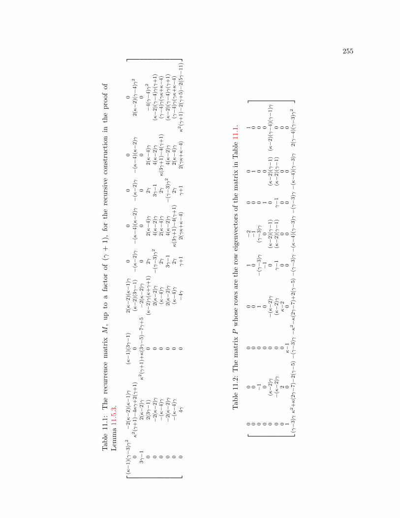
255

Tab

le11.

1:T

he

recu

rren

cem

atr

ixM

,u

pto

afa

ctor

of(γ

+1)

,fo

rth

ere

curs

ive

con

stru

ctio

nin

the

pro

ofof

Lem

ma

11.5

.3.

(κ−

1)(γ−

3)γ

2−

2(κ−

2)(κ−

1)γ

(κ−

1)(

3γ−

1)

2(κ−

2)(κ−

1)γ

00

00

0

0κ2(γ

+1)−

4κγ

+2(γ

+1)

0(κ−

2)(

3γ−

1)−

(κ−

2)γ

−(κ−

4)(κ−

2)γ

−(κ−

2)γ

−(κ−

4)(κ−

2)γ

2(κ−

2)(γ−

4)γ

2

3γ−

12(κ−

2)γ

κ2(γ

+1)+κ

(3γ−

5)−

7γ

+5

−2(κ−

2)γ

00

00

0

02(3γ−

1)

0(κ−

2)γ

(κ+γ

+1)

2γ

2(κ−

4)γ

2γ

2(κ−

4)γ

−4(γ−

4)γ

2

0−

2(κ−

2)γ

02(κ−

2)γ

−(γ−

3)γ

24(κ−

2)γ

3γ−

14(κ−

2)γ

(κ−

2)(γ−

4)γ

(γ+

1)

0−

(κ−

4)γ

0(κ−

4)γ

2γ

2(κ−

4)γ

2γ

κ(3γ

+1)−

4(γ

+1)

(γ−

4)γ

(γκ

+κ−

4)

0−

2(κ−

2)γ

02(κ−

2)γ

3γ−

14(κ−

2)γ

−(γ−

3)γ

24(κ−

2)γ

(κ−

2)(γ−

4)γ

(γ+

1)

0−

(κ−

4)γ

0(κ−

4)γ

2γ

κ(3γ

+1)−

4(γ

+1)

2γ

2(κ−

4)γ

(γ−

4)γ

(γκ

+κ−

4)

04γ

0−

4γ

γ+

12(γκ

+κ−

4)

γ+

12(γκ

+κ−

4)

κ2(γ

+1)−

2(γ

+5)−

2(5γ−

11)

Tab

le11.

2:T

he

matr

ixP

wh

ose

row

sar

eth

ero

wei

genvec

tors

ofth

em

atri

xin

Tab

le11

.1.

0

00

01

−2

00

10

00

00

−1

01

00

−1

01

−(γ−

3)γ

(γ−

3)γ

00

00

00

0−

10

10

00

(κ−

2)γ

0−

(κ−

2)γ

0(κ−

2)(γ−

1)

0(κ−

2)(γ−

1)

(κ−

2)(γ−

4)(γ−

1)γ

0−

(κ−

2)γ

0(κ−

2)γ

γ−

1(κ−

2)(γ−

1)

γ−

1(κ−

2)(γ−

1)

00

20

κ−

20

00

00

10

κ−

10

00

00

0(γ−

3)γ

κ2+κ

(2γ−

7)−

2(γ−

5)−

(γ−

3)γ−κ2−κ

(2γ−

7)+

2(γ−

5)−

(γ−

3)γ−

(κ−

4)(γ−

3)γ−

(γ−

3)γ−

(κ−

4)(γ−

3)γ

2(γ−

4)(γ−

3)γ

2

256

Figure 11.4: Quaternary gadget used in the interpolation construction below. Allvertices are assigned 〈−(κ− 1)γ, γ, 1〉.

Lemma 11.5.3. Suppose κ ≥ 3 is the domain size and a, b, c ∈ C. Let 〈a, b, c〉 be a succinct ternary

signature of type τ3. If a+ (κ− 1)b = 0 and b2 − 4bc− (κ− 3)c2 = 0, then

〈a, b, c〉 = c〈−(κ− 1)(2 + ε√κ+ 1), 2 + ε

√κ+ 1, 1〉,

where ε = ±1, and Pl-Holantκ(〈a, b, c〉) is #P-hard unless c = 0, in which case, the problem is

computable in polynomial time.

Proof. If c = 0, then a = b = c = 0 so the output is always 0. Otherwise, c 6= 0. Up to a

nonzero factor of c, 〈a, b, c〉 can be written as 〈−(κ − 1)(2 + ε√κ+ 1), 2 + ε

√κ+ 1, 1〉 under the

given assumptions, where ε = ±1.

Suppose κ = 3. If ε = −1, then we have 〈0, 0, 1〉 = AD3 and we are done by Theorem 10.2.7.

Otherwise, ε = 1 and we have 〈8,−4,−1〉. Let T = 13

[ 1 −2 −2−2 1 −2−2 −2 1

], which is an orthogonal matrix.

It follows from Theorem 3.2.2 and Lemma 9.2.6 that

Pl-Holant3(〈8,−4,−1〉) ≡ Pl-Holant3(T⊗3〈8,−4,−1〉) ≡ Pl-Holant3(〈0, 0, 1〉),

so again we are done by Theorem 10.2.7.

Now we suppose κ ≥ 4. Let g = 〈2, 0, 1, 0, 0, 0, 1, 0, 0〉 be a succinct quaternary signature

of type τ4. We reduce from Pl-Holantκ(g) to Pl-Holantκ(〈a, b, c〉). Then by Corollary 11.5.2,

Pl-Holantκ(〈a, b, c〉) is #P-hard. We write this signature as 〈−(κ−1)γ, γ, 1〉, where γ = 2+ε√κ+ 1.

Consider the gadget in Figure 11.4. We assign 〈−(κ−1)γ, γ, 1〉 to both vertices. By Lemma 9.2.3,

up to a nonzero factor of γ − 1, this gadget has the succinct quaternary signature f of type τ4,

where

f =⟨(κ− 1)(γ − 3)γ2, −(κ− 2)γ, 3γ − 1, 2γ, 3γ − 1, 2γ, −(γ − 3)γ2, 2γ, γ + 1

⟩.

257

Now consider the recursive construction in Figure 10.3. We assign f to all vertices. Let fs be the

succinct signature of type τ4 for the sth gadget in this recursive construction. The initial signature,

which is just two parallel edges, has the succinct signature f0 = 〈1, 0, 0, 0, 0, 0, 1, 0, 0〉 of type τ4.

We can express fs as M sf0, where M is the matrix in Table 11.1.

Consider an instance Ω of Pl-Holantκ(g). Suppose g appears n times in Ω. We construct from

Ω a sequence of instances Ωs of Pl-Holantκ(f) indexed by s ≥ 0. We obtain Ωs from Ω by replacing

each occurrence of g with the gadget fs.

We can express M as (γ − 1)3P−1ΛP , where P is the matrix in Table 11.2,

Λ = diag(−1,−1,−1,−1, κ− 2, κ− 2, κ− 1, κ− 1, λ),

and λ = (κ−2)(κ+2γ−4)(γ−1)2

. The rows of P are linearly independent since

det(P ) = (κ− 1)(κ− 2)2(γ − 1)6(γ − 3)3γ 6= 0.

For 1 ≤ i ≤ 9, let ri be the ith row of P . Notice that the initial signature f0 and the target

signature g are orthogonal to the same set of row eigenvectors of M , namely r1, r2, r3, r5, r7, r9.

Up to a common factor of (γ−1)3, the eigenvalues for M corresponding to r4, r6, and r8 (the three

row eigenvectors of M not orthogonal to f0) are −1, κ − 2, and κ − 1 respectively. Since κ ≥ 4,

κ−2 and κ−1 are relatively prime and greater than 1, so these three eigenvalues satisfy the lattice

condition. Thus by Lemma 11.3.6, we can interpolate g as desired.

Remark. Although the matrices in Table 11.1 and Table 11.2 seem large, they are probably the

smallest possible to succeed in this recursive quaternary construction. In fact, for quaternary

signatures one would normally expect these matrices to be even larger since there are typically

fifteen different entries in a domain invariant signature of arity 4.

The other failure condition of Lemma 11.5.1 is when both a+(κ−1)b = 0 and 2b+(κ−2)c = 0

hold. In this case, 〈a, b, c〉 = c〈(κ−1)(κ−2),−(κ−2), 2〉. If this signature is connected to 〈1〉, then

the first entry of the resulting succinct binary signature of type τ2 is (κ−1)(κ−2)·1−(κ−2)·(κ−1) =

258

0 while the second entry is −(κ− 2) · 2 + 2 · (κ− 2) = 0. That is, the resulting binary signature is

identically zero. This suggests we apply a holographic transformation such that the support of the

resulting signature is only on κ− 1 of the domain elements.

If c = 0, then a = b = c = 0 and the signature is trivial. Otherwise, c 6= 0. If κ = 3, then up to

a nonzero factor of c, this signature further simplifies to 〈2,−1, 2〉, which is tractable by case 3 of

Corollary 11.1.3. Otherwise κ ≥ 4, and we show the problem is #P-hard.

Lemma 11.5.4. Suppose κ ≥ 4 is the domain size. Let f = 〈(κ − 1)(κ − 2),−(κ − 2), 2〉 be a

succinct ternary signature of type τ3. Then Pl-Holantκ(f) is #P-hard.

Proof. Consider the matrix T =[

1 11 T ′

]∈ GLκ(C), where T ′ = yJκ−1 + (x − y)Iκ−1 with x =

−κ+√κ−1√

κ+1and y = 1√

κ+1. After scaling by 1√

κ, we claim that T is an orthogonal matrix.

Let ri be the ith row of 1√κT . First we compute the diagonal entries of 1

κTTᵀ. Clearly r1r

ᵀ1 = 1.

For 2 ≤ i ≤ κ, we have

rirᵀi =

1

κ

[1 + x2 + (κ− 2)y2

]=

1

κ

[1 +

(κ+√κ− 1)2

(√κ+ 1)2

+κ− 2

(√k + 1)2

]= 1.

Now we compute the off-diagonal entries. For 2 ≤ i ≤ κ, we have

r1rᵀi =

1

κ[1 + x+ (κ− 2)y] =

1

κ

[1− κ+

√κ− 1√

κ+ 1+

κ− 2√κ+ 1

]= 0.

For 2 ≤ i < j ≤ κ, we have

rirᵀj =

1

κ

[1 + 2xy + (κ− 3)y2

]=

1

κ

[1− 2(κ+

√κ− 1)

(√κ+ 1)2

+κ− 3

(√k + 1)2

]= 0.

This proves the claim.

We apply a holographic transformation by T to the signature f to obtain f = T⊗3f , which does

not change the complexity of the problem by Lemma 3.2.2. Since the first row of T is a row of all

1’s, the output of f on any input containing the first domain element is 0. When restricted to the

remaining κ− 1 domain elements, f is domain invariant and symmetric, so it can be expressed as

a succinct ternary signature of type τ3.

259

Up to a nonzero factor of κ3

(√κ+1)2

, it can be verified that f = 〈−(κ − 2)(2 +√κ), 2 +

√κ, 1〉.

One way to do this is as follows. We write f = 〈a, b, 2〉 and T =[

1 11 T ′

]∈ GLκ(C), where

T ′ = yJκ−1 + (x− y)Iκ−1. The entries of f are polynomials in κ with coefficients from Z[a, b, x, y].

The degree of these polynomials is at most 3 since the arity of f is 3. After computing the entries of

f for domain sizes 3 ≤ κ ≤ 6 as elements in Z[a, b, x, y], we interpolate the entries of f as elements

in (Z[a, b, x, y])[κ]. Then replacing a, b, x, y with their actual values gives the claimed expression

for the signature.

Since κ ≥ 4, f is #P-hard by Lemma 11.5.3, which completes the proof.

At this point, we have achieved the broader goal of this section. For any a, b, c ∈ C and domain

size κ ≥ 3, either Pl-Holantκ(〈a, b, c〉) is computable in polynomial time, or Pl-Holantκ(〈a, b, c〉) is

#P-hard, or we can use 〈a, b, c〉 to construct 〈1〉 (i.e. the reduction Pl-Holantκ(〈a, b, c, 〉, 〈1〉 ≤T

Pl-Holantκ(〈a, b, c〉) holds). However, Lemma 11.5.4 is easily generalized and this generalization

turns out to be necessary to obtain our dichotomy.

Recall that connecting f = 〈(κ − 1)(κ − 2),−(κ − 2), 2〉 to 〈1〉 results in an identically zero

signature. This suggests that we consider the more general signature f = α〈1〉⊗3+βf for any α ∈ C

and any nonzero β ∈ C since this does not change the complexity (as we argue in Corollary 11.5.5).

For any a, b, c ∈ C satisfying B = 0 (cf. (9.2.2)), if α = 2b+(κ−2)cκ and β = −b+c

κ , then f = 〈a, b, c〉.

We note that the condition B = 0 can also be written as (κ − 2)(b − c) = b − a. We now prove a

dichotomy for the signature f .

Corollary 11.5.5. Suppose κ ≥ 3 is the domain size and a, b, c ∈ C. Let 〈a, b, c〉 be a succinct

ternary signature of type τ3. If B = 0, then Pl-Holantκ(〈a, b, c〉) is #P-hard unless b = c or κ = 3,

in which case, the problem is computable in polynomial time.

Proof. If b = c, then by B = 0, we have a = b = c, which means the signature is degenerate and

the problem is trivially tractable. If κ = 3, then a = c and the problem is tractable by case 3 of

Corollary 11.1.3. Otherwise b 6= c and κ ≥ 4.

Since B = 0, it can be verified that

〈a, b, c〉 =2b+ (κ− 2)c

κ〈1〉⊗3 +

−b+ c

κf, where f = 〈(κ− 1)(κ− 2),−(κ− 2), 2〉.

260

We show that Pl-Holantκ(〈a, b, c〉) is #P-hard iff Pl-Holantκ(f) is. Since Pl-Holantκ(f) is #P-hard

by Lemma 11.5.4, this proves the result.

Let G = (V,E) be a connected planar 3-regular graph with n = |V | and m = |E|. We can

view Holantκ(G; 〈a, b, c〉) as a sum of 2n Holant computations using the signatures α〈1〉⊗3 and βf .

Each of these Holant computations considers a different assignment of either α〈1〉⊗3 or βf to each

vertex. Since connecting f to 〈1〉 gives an identically zero signature, if any connected signature

grid contains both α〈1〉⊗3 and βf , then that particular Holant computation is 0. This is because a

vertex of degree three assigned 〈1〉⊗3 is equivalent to three vertices of degree one connected to the

same three neighboring vertices and each assigned 〈1〉. There are only two possible assignments

that could be nonzero. If all vertices are assigned α〈1〉⊗3, then the Holant is αnκm. Otherwise,

all vertices are assigned βf and the Holant is βn Holantκ(G; f). Thus, Holantκ(G;α〈1〉⊗3 + βf) =

αnκm + βn Holantκ(G; f). Since β 6= 0, one can solve for either Holant value given the other.

11.6 Interpolating All Binary Signatures of Type τ2

In this section, we show how to interpolate all binary succinct signatures of type τ2 in most settings.

We use two general techniques to achieve this goal. In Subsection 11.6.2, we use a generalization

of the anti-gadget technique that creates a multitude of gadgets. They are so numerous that one

is most likely to succeed. In Subsection 11.6.3, we introduce a new technique called Eigenvalue

Shifted Triples (EST). These generalize the technique of Eigenvalue Shifted Pairs from [93], and we

use EST to interpolate binary succinct signatures in cases where the anti-gadget technique cannot

handle. There are a few isolated problems for which neither technique works. However, these

problems are easily handled separately in Lemma 11.6.1 in Subsection 11.6.1.

From Section 11.5, every problem fits into one of three cases: either (1) the problem is tractable,

(2) the problem is #P-hard, or (3) we can construct the succinct unary signature 〈1〉 of type τ1.

Thus, many results in this section assume that 〈1〉 is available.

261

11.6.1 Specific Cases

For some settings of a, b, c ∈ C, Lemma 11.6.4 and Lemma 11.6.12 do not apply. However, these

settings are easily handled on a case-by-case basis.

Lemma 11.6.1. Suppose κ ≥ 3 is the domain size. Let F be a signature set containing the succinct

unary signature 〈1〉 of type τ1 and any of the following succinct ternary signatures of type τ3:

1. 〈κ− 2± iκ√

2(κ− 2), κ− 2,−2〉;

2. 〈(κ− 2)2 ± iκ√κ2 − 4,−2(κ− 2), 4〉;

3. 〈−(2κ− 3)[2(κ− 2)± iκ

√2(κ− 2)

],−2(κ− 3)(κ− 2)± iκ

√2(κ− 2), 4(2κ− 3)〉 with κ 6= 4;

4. 〈−κ2 + 2, 2, 2〉;

5. 〈κ2 − 6κ+ 6,−2(κ− 3), 6〉;

6. 〈(κ− 3)(κ− 2)2 ± iκ(2κ− 3)√κ2 − 4,−3(κ− 2)2 ∓ iκ

√κ2 − 4, 2(5κ− 6)〉;

7. 〈−(κ− 1)[5(κ− 2)± 3iκ

√2(κ− 2)

],−(κ− 2)(3κ− 5)± iκ

√2(κ− 2), 9κ− 10〉;

8. 〈(κ− 1)[(κ− 2)(2κ+ 3)± 3κ

√κ2 − 5κ+ 6

], (κ− 3)(κ− 2)∓ κ

√κ2 − 5κ+ 6,−5κ+ 6〉;

9. 〈(κ− 1)[(κ− 2)(2κ− 7)± 3iκ

√κ2 − κ− 2

],−(κ− 2)(5κ− 7)∓ iκ

√κ2 − κ− 2, 13κ− 14〉;

10. 〈1, 0,−2〉 with κ = 3;

11. 〈±i√

2, 0, 1〉 with κ = 3;

12. 〈−1± i√

2, 0, 1〉 with κ = 3;

13. 〈−1± 3i√

3, 0, 2〉 with κ = 3;

Then

Pl-Holantκ(F ∪ 〈x, y〉) ≤T Pl-Holantκ(F)

for any x, y ∈ C, where 〈x, y〉 is a succinct binary signature of type τ2.

Proof. In each case, we use the recursive construction in Figure 10.4. We simply state which

gadget we use, the signature of that gadget, and the eigenvalues of its associated recurrence matrix

(cf. Lemma 10.3.2). Then the result easily follows from Corollary 10.3.3 as the eigenvalues have

distinct complex norms.

We use three possible gadgets, which are in Figure 11.6a, Figure 9.7c, and Figure 9.8c. The

signatures for the last two gadgets are given by Lemma 9.2.7 and Lemma 9.2.8 respectively.

262

1. For 〈κ − 2 ± iκ√

2(κ− 2), κ − 2,−2〉, we first use the gadget in Figure 9.7c. Let γ =

±i√

2(κ− 2). Up to a nonzero factor of (γ−2)7γ2(γ+2)3

64 , the signature of the gadget is 〈−1, 1〉,

which means the eigenvalues are κ− 2 and −2. If κ 6= 4, then these eigenvalues have distinct

complex norms. Otherwise, κ = 4 and we use the gadget in Figure 9.8c. Up to a factor of

±65536i, the signature of this gadget is 〈1,−3〉, which means the eigenvalues are −8 and 4.

2. For 〈(κ − 2)2 ± iκ√κ2 − 4,−2(κ − 2), 4〉, we first use the gadget in Figure 9.7c. Let γ =

±i√κ2 − 4. Up to a nonzero factor of −4(κ−2)κ3(κ2−4γ−8), the signature of this gadget is

〈κ2−6κ+ 4,−2(κ−4)〉, which means the eigenvalues are −(κ−2)2 and κ2−4k−4. If κ ≥ 5,

then these eigenvalues have opposite signs but cannot be the negative of each other. Thus,

they have distinct complex norms. The same conclusion holds for κ = 3 by direct inspection.

Otherwise, κ = 4 and we use the gadget in Figure 9.8c. Up to a factor of 2097152, the

signature of this gadget is 〈5, 1〉, which means the eigenvalues are 8 and 4.

3. For 〈−(2κ− 3)[2(κ− 2)± iκ

√2(κ− 2)

],−2(κ− 3)(κ− 2)± iκ

√2(κ− 2), 4(2κ− 3)〉, we have

κ 6= 4. We use the gadget in Figure 9.7c. Let γ = ±i√

2(κ− 2). Up to a nonzero factor of

−4(κ−2)κ6(3κ−4)(4κ2−28κ+41−4γ(2κ−5)), the signature of the gadget is 1κ〈3κ−4, κ−4〉,

which means the eigenvalues are κ− 2 and 2.

4. For 〈−κ2 + 2, 2, 2〉, we use the gadget in Figure 9.7c. Up to a nonzero factor of (κ− 2)κ5, the

signature for this gadget is 〈κ2 + 2κ− 4,−4〉, which means the eigenvalues are (κ− 2)κ and

κ(κ+ 2).

5. For 〈κ2 − 6κ + 6,−2(κ − 3), 6〉, we use the gadget in Figure 9.7c. Up to a nonzero factor of

(κ− 2)κ5, the signature for this gadget is 〈κ2 + 2κ− 4,−4〉, which means the eigenvalues are

(κ− 2)κ and κ(κ+ 2).

6. For 〈(κ−3)(κ−2)2±iκ(2κ−3)√κ2 − 4,−3(κ−2)2∓iκ

√κ2 − 4, 2(5κ−6)〉, we use the gadget in

Figure 9.7c. Let γ = ±i√κ2 − 4. Up to a nonzero factor of (γ−2)2(γ+2)2(κ−2)κ[7κ2+60κ−

164+8γ(3κ−10)], the signature of the gadget is 〈−κ4+6κ3+4κ2−24κ+16, 2(κ3−2κ2−8κ+8)〉,

which means the eigenvalues are λ1 = (κ− 2)κ(κ2 + 2κ− 4) and λ2 = −κ(κ+ 2)(κ2− 6κ+ 4).

For 3 ≤ κ ≤ 5, one can directly check that these eigenvalues have distinct complex norms.

For κ ≥ 6, we have λ2 < 0, so these eigenvalues have the same complex norm preciously when

263

λ1 = −λ2. However, λ1 + λ2 = 4κ3 6= 0, so the eigenvalues have distinct complex norms.

7. For 〈−(κ− 1)[5(κ− 2)± 3iκ

√2(κ− 2)

],−(κ− 2)(3κ− 5)± iκ

√2(κ− 2), 9κ− 10〉, we first

use the gadget in Figure 9.7c. Let γ = ±i√

2(κ− 2). Up to a nonzero factor of −(κ −

2)(κ− 1)κ5[81κ2− 756κ+ 1252− 24(9κ− 26)γ], the signature of this gadget is 〈5κ− 6, κ− 6〉,

which means the eigenvalues are κ − 2 and 4. If κ 6= 6, then these eigenvalues have distinct

complex norms. Otherwise, κ = 6 and we use the gadget in Figure 9.8c. Up to a factor

of −17199267840(1169 ± 450i√

2), the signature of this gadget is 〈7, 13〉, which means the

eigenvalues are 72 and −6.

8. For 〈(κ− 1)[(κ− 2)(2κ+ 3)± 3κ

√κ2 − 5κ+ 6

], (κ− 3)(κ− 2)∓κ

√κ2 − 5κ+ 6,−5κ+ 6〉, we

first use the gadget in Figure 9.7c. Let γ = ±√κ2 − 5κ+ 6. Up to a factor of (κ − 2)(κ −

1)κ5[313κ2−1500κ+1764−24(13κ−30)γ], the signature of this gadget is 〈κ3−3κ2+3,−κ+3〉,

which means the eigenvalues are λ1 = (κ − 2)2κ and λ2 = κ(κ2 − 3κ + 1). If κ ≥ 4, these

eigenvalues are positive, so they have the same complex norm preciously when λ1 = λ2.

However, λ1−λ2 = −(κ−3)κ 6= 0, so the eigenvalues have distinct complex norms. Otherwise,

κ = 3 and we use the gadget in Figure 9.8c. Up to a factor of 9565938, the signature of this

gadget is 〈5, 2〉, which means the eigenvalues are 9 and 3.

9. For 〈(κ− 1)[(κ− 2)(2κ− 7)± 3iκ

√κ2 − κ− 2

],−(κ− 2)(5κ− 7)∓ iκ

√κ2 − κ− 2, 13κ− 14〉,

we use the gadget in Figure 9.7c. Let γ = ±i√κ2 − κ− 2. Up to a nonzero factor of

(κ−2)(κ−1)κ5[119κ2 +76κ−772+24(5κ−22)γ], the signature of this gadget is 〈−κ3 +7κ2−

4κ−3, 2κ2−7κ−3〉, which means the eigenvalues are λ1 = (κ−2)κ2 and λ2 = −κ(k2−5κ−3).

For 3 ≤ κ ≤ 5, one can directly check that these eigenvalues have distinct complex norms.

For κ ≥ 6, we have λ2 < 0, so these eigenvalues have the same complex norm preciously when

λ1 = −λ2. However, λ1 +λ2 = 3κ(κ+1) 6= 0, so the eigenvalues have distinct complex norms.

10. For 〈1, 0,−2〉 with κ = 3, we use the gadget in Figure 9.7c. Up to a factor of 3, the signature

of this gadget is 〈11,−4〉, which means the eigenvalues are 3 and 15.

11. For 〈±i√

2, 0, 1〉 with κ = 3, we use the gadget in Figure 11.6a. The signature of this gadget

is 〈±i√

2, 1〉, which means the eigenvalues are 2± i√

2 and −1± i√

2.

12. For 〈−1 ± i√

2, 0, 1〉 with κ = 3, we use the gadget in Figure 11.6a. The signature of this

264

gadget is 〈−1± i√

2, 1〉, which means the eigenvalues are 1± i√

2 and −2± i√

2.

13. For 〈−1± 3i√

3, 0, 2〉 with κ = 3, we use the gadget in Figure 9.7c. Up to a factor of 72, the

signature of this gadget is 13〈25±13

√3,−5±i

√3〉, which means the eigenvalues are 5(1±i

√3)

and 2(5± 2√

3).

11.6.2 E Pluribus Unum

In this subsection, we use Lemma 10.1.3 to prove our interpolation results. The main technical

difficulty is to satisfy the third condition of Lemma 10.1.3, which is to prove that some recurrence

matrix (that defines a sequence of gadgets) has infinite order up to a scalar. When the matrix has

a finite order up to a scalar, we can utilize this failure condition to our advantage by constructing

an anti-gadget (cf. Chapter 5), which is the “last” gadget with a distinct signature (up to a scalar)

in the infinite sequence of gadgets. To make sure that we construct a multitude of nontrivial

gadgets without cancellation, we put the anti-gadget inside another gadget (contrast the gadget in

Figure 11.5 with the gadget in Figure 11.6b). From among this plethora of gadgets, at least one

must succeed under the right conditions.

Although this idea works quite well in that some gadget among those constructed does succeed,

we still must prove that one such gadget succeeds in every setting. We aim to exhibit a recurrence

matrix whose ratio of eigenvalues is not a root of unity. We consider three related recurrence

matrices at once. The next two lemmas consider two similar situations involving the eigenvalues

of three such matrices. When applied, these lemmas show that some recurrence matrix must have

eigenvalues with distinct complex norms, even though exactly which one among them succeeds may

depend on the parameters in a complicated way.

Lemma 11.6.2. Let d0, d1, d2,Ψ ∈ C. If d0, d1, and d2 have the same argument but are distinct,

then for all ρ ∈ R, there exists i ∈ 0, 1, 2 such that |Ψ + di| 6= ρ.

Proof. Assume to the contrary that there exists ρ ∈ R such that |Ψ +di| = ρ for every i ∈ 0, 1, 2.

In the complex plane, consider the circle centered at the origin of radius ρ. Each Ψ+di is a distinct

point on this circle as well as a distinct point on a common line through Ψ. However, the line

intersects the circle in at most two points, a contradiction.

265

Lemma 11.6.3. Let d0, d1, d2,Ψ ∈ C. If d0, d1, and d2 have the same complex norm but are

distinct and Ψ 6= 0, then for all ρ ∈ R, there exists i ∈ 0, 1, 2 such that |Ψ + di| 6= ρ.

Proof. Let ` = |d0|. Assume to the contrary that there exists ρ ∈ R such that |Ψ+di| = ρ for every

i ∈ 0, 1, 2. In the complex plane, consider the circle centered at the origin of radius ρ and the

circle centered at Ψ of radius `. Since Ψ 6= 0, these circles are distinct. Each Ψ + di is a distinct

point on both circles. However, these circles intersect in at most two points, a contradiction.

Now we use Lemma 11.6.2 and Lemma 11.6.3 as well as our generalization of the anti-gadget

technique to establish a crucial lemma.

Lemma 11.6.4. Suppose κ ≥ 3 is the domain size and a, b, c, ω ∈ C. Let F be a set of signatures

containing the succinct binary signature 〈ω + κ − 1, ω − 1〉 of type τ2 and the succinct ternary

signature 〈a, b, c〉 of type τ3. If the following three conditions are satisfied:

1. ω 6∈ 0,±1,

2. B 6= 0, and

3. at least one of the following holds:

(i) C = 0 or

(ii) C2 = ω2`B2 for some ` ∈ 0, 1 but either C2 6= A2 or κ 6= 3,

then

Pl-Holantκ(F ∪ 〈x, y〉) ≤T Pl-Holantκ(F)

for any x, y ∈ C, where 〈x, y〉 is a succinct binary signature of type τ2.

We use this lemma to establish that various 2-by-2 recurrence matrices have infinite order

modulo scalars. When applied, ω will be the ratio of two eigenvalues, one of which is a multiple of

B or B2 by a nonzero function of κ.

Proof of Lemma 11.6.4. Let Φ = C2

B2 and Ψ = (κ−2)A2

B2 . Consider the recursive construction in

Figure 10.4. After scaling by a nonzero factor of κ, we assign f = 1κ〈ω+κ−1, ω−1〉 to every vertex.

Let fs be the succinct binary signature of type τ2 for the sth gadget in this construction. We can

express fs as M s [ 10 ], where M = 1

κ

[ω+κ−1 (κ−1)(ω−1)ω−1 (κ−1)ω+1

]=[

1 1−κ1 1

][ ω 0

0 1 ][

1 1−κ1 1

]−1by Lemma 10.3.2.

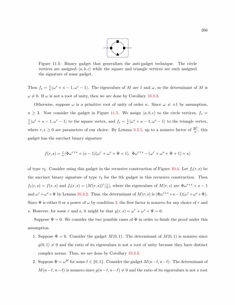
266

Figure 11.5: Binary gadget that generalizes the anti-gadget technique. The circlevertices are assigned 〈a, b, c〉 while the square and triangle vertices are each assignedthe signature of some gadget.

Then fs = 1κ〈ω

s + κ − 1, ωs − 1〉. The eigenvalues of M are 1 and ω, so the determinant of M is

ω 6= 0. If ω is not a root of unity, then we are done by Corollary 10.3.3.

Otherwise, suppose ω is a primitive root of unity of order n. Since ω 6= ±1 by assumption,

n ≥ 3. Now consider the gadget in Figure 11.5. We assign 〈a, b, c〉 to the circle vertices, fr =

1κ〈ω

r + κ − 1, ωr − 1〉 to the square vertex, and fs = 1κ〈ω

s + κ − 1, ωs − 1〉 to the triangle vertex,

where r, s ≥ 0 are parameters of our choice. By Lemma 9.2.5, up to a nonzero factor of B2

κ , this

gadget has the succinct binary signature

f(r, s) = 1κ〈Φω

r+s + (κ− 1)(ωr + ωs + Ψ + 1), Φωr+s − (ωr + ωs + Ψ + 1) + κ〉

of type τ2. Consider using this gadget in the recursive construction of Figure 10.4. Let ft(r, s) be

the succinct binary signature of type τ2 for the tth gadget in this recursive construction. Then

f1(r, s) = f(r, s) and ft(r, s) = (M(r, s))t [ 10 ], where the eigenvalues of M(r, s) are Φωr+s + κ − 1

and ωr+ωs+Ψ by Lemma 10.3.2. Thus, the determinant of M(r, s) is (Φωr+s+κ−1)(ωr+ωs+Ψ).

Since Φ is either 0 or a power of ω by condition 3, the first factor is nonzero for any choice of r and

s. However, for some r and s, it might be that g(r, s) = ωr + ωs + Ψ = 0.

Suppose Ψ = 0. We consider the two possible cases of Φ in order to finish the proof under this

assumption.

1. Suppose Φ = 0. Consider the gadget M(0, 1). The determinant of M(0, 1) is nonzero since

g(0, 1) 6= 0 and the ratio of its eigenvalues is not a root of unity because they have distinct

complex norms. Thus, we are done by Corollary 10.3.3.

2. Suppose Φ = ω2` for some ` ∈ 0, 1. Consider the gadget M(n−`, n−`). The determinant of

M(n−`, n−`) is nonzero since g(n−`, n−`) 6= 0 and the ratio of its eigenvalues is not a root

267

of unity because they have distinct complex norms. Thus, we are done by Corollary 10.3.3.

Otherwise, Ψ 6= 0. We claim that g(r, s) = 0 can hold for at most one choice of r, s ∈ Zn (modulo

the swapping of r and s). To see this, consider r1, s1, r2, s2 such that g(r1, s1) = 0 = g(r2, s2). Then

ωr1 + ωs1 = −Ψ = ωr2 + ωs2 . By taking complex norms and applying the law of cosines, we have

cos θ1 = cos θ2, where θj = arg(ωsj−rj ) is the angle from ωrj to ωsj for j ∈ 1, 2. Thus, θ1 = ±θ2.

Since Ψ 6= 0, we have θ1 6= ±π. If θ1 = θ2, then ωr1(1 + eiθ1) = ωr2(1 + eiθ1). Since θ1 6= ±π, the

factor 1 + eiθ1 is nonzero. After dividing by this factor, we conclude that r1 = r2 and thus s1 = s2.

Otherwise, θ1 = −θ2. Then ωr1(1 + eiθ1) = ωs2(1 + eiθ1) and we conclude that r1 = s2 and s1 = r2.

This proves the claim.

Suppose n ≥ 4 and let S0 = (0, 0), (1, n − 1), (2, n − 2) and S1 = (1, 1), (2, 0), (3, n − 1).

Then g(r, s) = 0 holds for at most one (r, s) ∈ S0 ∪ S1. In particular, g(r, s) is either nonzero for

all (r, s) ∈ S0 or nonzero for all (r, s) ∈ S1. Pick j ∈ 0, 1 such that g(r, s) is nonzero for all

(r, s) ∈ Sj . By Lemma 11.6.2 with di = (ωi + ω−i)ωj and ρ = |Φω2j + κ − 1|, there exists some

(r, s) ∈ Sj such that the eigenvalues of M(r, s) have distinct complex norms, so we are done by

Corollary 10.3.3.

Otherwise, n = 3. We consider the two possible cases of Φ in order to finish the proof.

1. Suppose Φ = 0. Let Sj = (0, j), (1, j + 1), (2, j + 2). Then g(r, s) = 0 holds for at most one

(r, s) ∈ S0 ∪ S1. In particular, g(r, s) is either nonzero for all (r, s) ∈ S0 or nonzero for all

(r, s) ∈ S1. Pick j ∈ 0, 1 such that g(r, s) is nonzero for all (r, s) ∈ Sj . By Lemma 11.6.3

with di = (1 + ωj)ωi and ρ = κ− 1, there exists some (r, s) ∈ Sj such that the eigenvalues of

M(r, s) have distinct complex norms, so we are done by Corollary 10.3.3.

2. Suppose Φ = ω2` for some ` ∈ 0, 1 but either C2 6= A2 or κ 6= 3. Note that this is equivalent

to Φ 6= Ψ or κ 6= 3. Consider the set S = (0, 0), (0, 1), (0, 2), (1, 1), (1, 2), (2, 2). If there

exists some (r, s) ∈ S such that g(r, s) 6= 0 and the eigenvalues of M(r, s) have distinct

complex norms, then we are done by Corollary 10.3.3.

Otherwise, for every (r, s) ∈ S, either g(r, s) = 0 or the eigenvalues of M(r, s) have the same

268

complex norm. If the latter condition were to always hold, then we would have

|2 + Ψ| =∣∣∣ω2` + κ− 1

∣∣∣ = |−1 + Ψ| ,∣∣2ω2 + Ψ∣∣ =

∣∣∣ω2`+1 + κ− 1∣∣∣ =

∣∣−ω2 + Ψ∣∣ , and

|2ω + Ψ| =∣∣∣ω2`+2 + κ− 1

∣∣∣ = |−ω + Ψ| ,

where each equality corresponds to one of the six M(r, s) having eigenvalues of equal complex

norm for (r, s) ∈ S. Of the six equalities, at most one may not hold since g(r, s) = 0 for at

most one (r, s) ∈ S. Since n = 3, two of the three terms of the form |ω2`+m + κ− 1| must be

equal, so we can write the stronger condition

∣∣∣2ω2 + Ψω`∣∣∣ = |ω + κ− 1| =

∣∣∣−ω2 + Ψω`∣∣∣= (11.6.4)∣∣∣2ω + Ψω`

∣∣∣ =∣∣ω2 + κ− 1

∣∣ =∣∣∣−ω + Ψω`

∣∣∣ .As it is, one of the horizontal equalities in (11.6.4) may not hold. However, even without one

of these equalities, we can still reach a contradiction.

We show that Ψω` ∈ R even if one of the equalities in (11.6.4) does not hold. In fact, either the

left or the right half of the equalities in (11.6.4) hold. In the first case, |2ω2+Ψω`| = |2ω+Ψω`|

holds and we get Ψω` ∈ R. Similarly in the second case, |−ω2 +Ψω`| = |−ω+Ψω`| holds and

we get Ψω` ∈ R as well. Next, we use real and imaginary parts to calculate the complex norms

even if one of the equalities in (11.6.4) does not hold. Either the top half of the equalities

hold and thus |2ω2 + Ψω`| = |−ω2 + Ψω`|, or the bottom half of the equalities hold and thus

|2ω+ Ψω`| = |−ω+ Ψω`|. In any case, it readily follows that Ψω` = 1. This implies Ψ = ω2`,

269

(a) (b)

Figure 11.6: Binary gadgets used to interpolate any succinct binary signature of typeτ2. The circle vertices are assigned 〈a, b, c〉 and the square vertex is assigned 〈1〉.

so we can rewrite (11.6.4) as

√3 = |ω + κ− 1| =

√3

=

√3 =

∣∣ω2 + κ− 1∣∣ =√

3,

where at most one equation may not hold. This forces κ = 3. However, Φ = ω2` = Ψ and

κ = 3 is a contradiction.

The previous lemma is strong enough to handle the typical case.

Lemma 11.6.5. Suppose κ ≥ 3 is the domain size and a, b, c ∈ C. Let F be a signature set

containing the succinct ternary signature 〈a, b, c〉 of type τ3 and the succinct unary signature 〈1〉 of

type τ1. If

1. B 6= 0,

2. C 6= 0,

3. C2 6= B2, and

4. either C2 6= A2 or κ 6= 3,

then

Pl-Holantκ(F ∪ 〈x, y〉) ≤T Pl-Holantκ(F)

for any x, y ∈ C, where 〈x, y〉 is a succinct binary signature of type τ2.

Proof. Let ω = CB , which is well-defined. Consider the gadget in Figure 11.6a. We assign 〈a, b, c〉

to the circle vertex and 〈1〉 to the square vertex. Up to a nonzero factor of Bκ , this gadget has the

270

succinct binary signature

κ

B〈a+ (κ− 1)b, 2b+ (κ− 2)c〉 = 〈ω + κ− 1, ω − 1〉

of type τ2. Then we are done by Lemma 11.6.4 with ` = 1 in case (ii) of condition 3.

If B = 0, then we already know the complexity by Corollary 11.5.5. The other failure conditions

from the previous lemma are:

C−B = κ[2b+ (κ− 2)c] = 0; (11.6.5)

C + B = 2a+ 2(2κ− 3)b+ (κ− 2)2c = 0; (11.6.6)

C = 0; (11.6.7)

κ = 3 and C− A = 0, or equivalently κ = 3 and b = 0; (11.6.8)

κ = 3 and C + A = 0, or equivalently κ = 3 and 2a+ 3b+ 4c = 0. (11.6.9)

Notice that these five failure conditions are linear in a, b, c.

By starting the proof with a different gadget, Lemma 11.6.4 can handle the first three failure

conditions. The last two failure conditions require a new idea, Eigenvalue Shifted Triples, which

we introduce in Subsection 11.6.3. In fact, these two cases are equivalent under an orthogonal

holographic transformation.

The next lemma considers the failure condition in (11.6.5). Note that C = B iff the signature

can be written as 〈2a,−(κ− 2)c, 2c〉 up to a factor of 2. The first excluded case in Lemma 11.6.6

is handled by Corollary 11.5.5 and the last two excluded cases are tractable by Corollary 11.1.4.

Lemma 11.6.6. Suppose κ ≥ 3 is the domain size and a, c ∈ C. Let F be a signature set containing

the succinct ternary signature 〈2a,−(κ− 2)c, 2c〉 of type τ3 and the succinct unary signature 〈1〉 of

type τ1. If

1. 2a 6= (κ− 1)(κ− 2)c,

2. 4a 6= (κ2 − 6κ+ 4)c, and

3. c 6= 0,

271

then

Pl-Holantκ(F ∪ 〈x, y〉) ≤T Pl-Holantκ(F)

for any x, y ∈ C, where 〈x, y〉 is a succinct binary signature of type τ2.

Proof. Note that when 2b = −(κ − 2)c, we have B = C = 2a − (κ − 1)(κ − 2)c by (11.6.5), which

is nonzero by condition 1 of the lemma. Let ω0 = 4a2 + (κ− 2)[4ac+ (2κ2 + κ− 2)c2] and assume

ω0 6= 0. Then let ω = B2

ω06= 0. By conditions 2 and 3, it follows that ω 6= 1. Also we note that

when 2b = −(κ − 2)c, we have 2A = 2a + (3κ − 2)c and 2C = 2a − (κ − 1)(κ − 2)c. By the same

conditions, 2 and 3, we have C2 6= A2. We further assume that ω 6= −1, which is equivalent to

8a2 − 4(κ− 2)2ac+ (κ− 2)(κ3 − 2κ2 + 6κ− 4)c2 6= 0.

Consider the gadget in Figure 11.6b. We assign 〈2a,−(κ − 2)c, 2c〉 to the vertices. Up to a

nonzero factor of ω0κ , this gadget has the succinct binary signature

κ

ω0〈4a2 + (κ− 1)(κ− 2)(3κ− 2)c2, −(κ− 2)[4ac− (κ2 − 6κ+ 4)c2]〉 = 〈ω + κ− 1, ω − 1〉

of type τ2. Then we are done by Lemma 11.6.4 with ` = 0 in case (ii) of condition 3.

Now we deal with the following exceptional cases.

1. If ω0 = 0, then 2a = −[κ − 2 ± iκ

√2(κ− 2)

]c. Up to a nonzero factor of −c, we have

−1c 〈2a,−(κ−2)c, 2c〉 = 〈κ−2±iκ

√2(κ− 2), κ−2,−2〉 and are done by case 1 of Lemma 11.6.1.

2. If 8a2 − 4(κ− 2)2ac+ (κ− 2)(κ3 − 2κ2 + 6κ− 4)c2 = 0, then 4a =[(κ− 2)2 ± iκ

√κ2 − 4

]c.

Up to a nonzero factor of c2 , we have

2

c〈2a,−(κ− 2)c, 2c〉 = 〈(κ− 2)2 ± iκ

√κ2 − 4,−2(κ− 2), 4〉

and are done by case 2 of Lemma 11.6.1.

The next lemma considers the failure condition in (11.6.6). Note that C = −B iff the signa-

ture can be written as 〈−2(2κ − 3)b − (κ − 2)2c, 2b, 2c〉 up to a factor of 2. The first excluded

case in Lemma 11.6.7 is handled by Corollary 11.5.5 and the last excluded case is tractable by

Corollary 11.1.7.

272

Lemma 11.6.7. Suppose κ ≥ 3 is the domain size and a, b ∈ C. Let F be a signature set containing

the succinct ternary signature 〈−2(2κ − 3)b − (κ − 2)2c, 2b, 2c〉 of type τ3 and the succinct unary

signature 〈1〉 of type τ1. If

1. 2b 6= −(κ− 2)c and

2. κ 6= 4 or 5b2 + 2bc+ c2 6= 0,

then

Pl-Holantκ(F ∪ 〈x, y〉) ≤T Pl-Holantκ(F)

for any x, y ∈ C, where 〈x, y〉 is a succinct binary signature of type τ2.

Proof. Note that when 2a = −2(2κ − 3)b − (κ − 2)2c, we have B = −C by (11.6.6) and 2B =

−κ[2b + (κ − 2)c], which is nonzero by condition 1 of the lemma. Let ω0 = 8(2κ − 3)b2 + (κ −

2)[8(κ− 3)bc+ (κ2 − 6κ+ 12)c2

]and assume ω0 6= 0. Then let ω = κ[2b+(κ−2)c]2

ω0. By condition 1,

ω 6= 0. It can be shown that κ[2b+ (κ− 2)c]2 = ω0 is equivalent to (b− c)[3b+ (κ− 3)c] = 0. Thus,

assume b 6= c and 3b 6= −(κ−3)c. Then ω 6= 1. Also we note that when 2a = −2(2κ−3)b−(κ−2)2c,

we have 2A = −κ[4b + (κ − 4)c] and 2C = κ[2b + (κ − 2)c]. By the same assumptions, b 6= c

and 3b 6= −(κ − 3)c, we have C2 6= A2. Further assume that ω 6= −1, which is equivalent to

2(5κ− 6)b2 + (κ− 2)[6(κ− 2)bc+ (κ2 − 4κ+ 6)c2] 6= 0.

Consider the gadget in Figure 11.6b. We assign 〈−2(2κ− 3)b− (κ− 2)2c, 2b, 2c〉 to the vertices.

Up to a nonzero factor of ω04 , this gadget has the succinct binary signature 1

ω0〈x, y〉 = 〈ω+κ−1, ω−1〉

of type τ2, where

x = 4(4κ2 − 9κ+ 6)b2 + (κ− 2)[4(κ− 2)(2κ− 3)bc+ (κ3 − 6κ2 + 16κ− 12)c2

]and

y = −4(κ− 2)[3b3 + (κ− 6)bc− (κ− 3)c2

].

Then we are done by Lemma 11.6.4 with ` = 0 in case (ii) of condition 3.

Now we deal with the following exceptional cases.

1. If ω0 = 0, then we have −4(2κ − 3)b =[2(κ − 3)(κ − 2) ± iκ

√2(κ− 2)

]c but κ 6= 4 by

273

condition 2 since otherwise ω0 = 8(5b2 + 2bc+ c2) 6= 0. Up to a nonzero factor of c2(2κ−3) ,

2(2κ− 3)

c〈−2(2κ− 3)b− (κ− 2)2c, 2b, 2c〉

= 〈−(2κ− 3)[2(κ− 2)∓ iκ

√2(κ− 2)

], −2(κ− 3)(κ− 2)∓ iκ

√2(κ− 2), 4(2κ− 3)〉

and are done by case 3 of Lemma 11.6.1.

2. If b = c, then up to a nonzero factor of c, we have 1c 〈−2(2κ − 3)b − (κ − 2)2c, 2b, 2c〉 =

〈−κ2 + 2, 2, 2〉 and are done by case 4 Lemma 11.6.1.

3. If 3b = −(κ−3)c, then up to a nonzero factor of c3 , we have 3

c 〈−2(2κ−3)b−(κ−2)2c, 2b, 2c〉 =

〈κ2 − 6κ+ 6,−2(κ− 3), 6〉 and are done by case 5 of Lemma 11.6.1.

4. If 2(5κ − 6)b2 + (κ − 2)[6(κ − 2)bc + (κ2 − 4κ + 6)c2] = 0, then −2(5κ − 6)b =[3(κ − 2)2 ±

iκ√κ2 − 4

]c. Up to a nonzero factor of c

5κ−6 ,

5κ− 6

c〈−2(2κ− 3)b− (κ− 2)2c, 2b, 2c〉

= 〈(κ− 3)(κ− 2)2 ± iκ(2κ− 3)√κ2 − 4, −3(κ− 2)2 ∓ iκ

√κ2 − 4, 2(5κ− 6)〉

and are done by case 6 of Lemma 11.6.1.

The next lemma considers the failure condition in (11.6.7). Note that C = 0 iff the signature

can be written as 〈−3(κ−1)b− (κ−1)(κ−2)c, b, c〉. The excluded case in Lemma 11.6.8 is handled

by Corollary 11.5.5.

Lemma 11.6.8. Suppose κ ≥ 3 is the domain size and b, c ∈ C. Let F be a signature set containing

the succinct ternary signature 〈−3(κ− 1)b− (κ− 1)(κ− 2)c, b, c〉 of type τ3 and the succinct unary

signature 〈1〉 of type τ1. If 2b 6= −(κ− 2)c, then

Pl-Holantκ(F ∪ 〈x, y〉) ≤T Pl-Holantκ(F)

for any x, y ∈ C, where 〈x, y〉 is a succinct binary signature of type τ2.

Proof. Note that when a = −3(κ−1)b− (κ−2)(κ−1)c, we have C = 0 and 2B = −κ[2b+(κ−2)c],

274

which is nonzero by assumption. Let ω0 = (9κ− 10)b2 + (κ− 2)[2(3κ− 5)bc+ (κ2 − 4κ+ 5)c2] and

assume ω0 6= 0. Then let ω = (κ−1)[2b+(κ−2)c]2

ω0. By assumption, ω 6= 0. Assume ω 6= 1, which is

equivalent to −(5κ−6)b2− (κ−3)(κ−2)(2b−c)c 6= 0. Further assume ω 6= −1, which is equivalent

to (13κ− 14)b2 + (κ− 2)[2(5κ− 7)bc+ (2κ2 − 7κ+ 7)c2] 6= 0.

Consider the gadget in Figure 11.6b. We assign 〈−3(κ−1)b−(κ−1)(κ−2)c, b, c〉 to the vertices.

Up to a nonzero factor of ω0, this gadget has the succinct binary signature 1ω0〈x, y〉 = 〈ω+κ−1, ω−1〉

of type τ2, where

x = (κ− 1)

3(3κ− 2)b2 + (κ− 2)[6bc+ (κ2 − 3κ+ 3)c2

]and

y = −(5κ− 6)b2 − (κ− 3)(κ− 2)(2b− c)c.

Then we are done by Lemma 11.6.4 via case (i) of condition 3.

Now we deal with the following exceptional cases.

1. If ω0 = 0, then −(9κ − 10)b = [(κ − 2)(3κ − 5) ± iκ√

2(κ− 2)]c. Up to a nonzero factor of

c9κ−10 , we have

9κ− 10

c〈−3(κ− 1)b− (κ− 1)(κ− 2)c, b, c〉

= 〈−(κ− 1)[5(κ− 2)∓ 3iκ

√2(κ− 2)

], −(κ− 2)(3κ− 5)∓ iκ

√2(κ− 2), 9κ− 10〉

and we are done by case 7 of Lemma 11.6.1.

2. If −(5κ−6)b2−(κ−3)(κ−2)(2b−c)c = 0, then −(5κ−6)b =[(κ−3)(κ−2)±κ

√κ2 − 5κ+ 6

]c.

Up to a nonzero factor of − c5κ−6 , we have

− 5κ− 6

c〈−3(κ− 1)b− (κ− 1)(κ− 2)c, b, c〉

= 〈(κ−1)[(κ− 2)(2κ+ 3)∓ 3κ

√κ2 − 5κ+ 6

], (κ−3)(κ−2)±κ

√κ2 − 5κ+ 6, −5κ+6〉

and are done by case 8 Lemma 11.6.1.

275

3. If (13κ− 14)b2 + (κ− 2)[2(5κ− 7)bc+ (2κ2 − 7κ+ 7)c2] = 0, then

−(13κ− 14)b =[(κ− 2)(5κ− 7)± iκ

√κ2 − κ− 2

]c.

Up to a nonzero factor of c13κ−14 , we have

13κ− 14

c〈−3(κ− 1)b− (κ− 1)(κ− 2)c, b, c〉

= 〈(κ−1)[(κ− 2)(2κ− 7)± 3iκ

√κ2 − κ− 2

], −(κ−2)(5κ−7)∓iκ

√κ2 − κ− 2, 13κ−14〉

and are done by case 9 of Lemma 11.6.1.

11.6.3 Eigenvalue Shifted Triples

To handle failure conditions (11.6.8) and (11.6.9) from Lemma 11.6.5, we need another technique.

We introduce an Eigenvalue Shifted Triple, which extends the concept of an Eigenvalue Shifted

Pair.

Definition 11.6.9 (Definition 4.6 in [93]). A pair of nonsingular matrices M,M ′ ∈ C2×2 is called

an Eigenvalue Shifted Pair if M ′ = M+δI for some nonzero δ ∈ C, and M has distinct eigenvalues.

Eigenvalue shifted pairs were used in [93] to show that interpolation succeeds in most cases

since these matrices correspond to some recursive gadget constructions and at least one of them

usually has eigenvalues with distinct complex norms. In [93], it is shown that the interpolation

succeeds unless the variables in question take real values. Then other techniques were developed to

handle the real case. We use Eigenvalue Shifted Pairs in a stronger way. We exhibit three matrices

such that any two form an Eigenvalue Shifted Pair. Provided these shifts are linearly independent

over R, this is enough to show that interpolation succeeds for both real and complex settings of the

variables. We call this an Eigenvalue Shifted Triple.

Definition 11.6.10. A trio of nonsingular matrices M0,M1,M2 ∈ C2×2 is called an Eigenvalue

Shifted Triple (EST) if M0 has distinct eigenvalues and there exist nonzero δ1, δ2 ∈ C satisfying

δ1δ26∈ R such that M1 = M0 + δ1I, and M2 = M0 + δ2I.

276

If M0, M1, and M2 form an Eigenvalue Shifted Triple, then any permutation of the matrices is

also an Eigenvalue Shifted Triple.

The proof of the next lemma is similar to the proof of Lemma 4.7 in [94].

Lemma 11.6.11. Suppose α, β, δ1, δ2 ∈ C. If α 6= β, δ1, δ2 6= 0, and δ1δ26∈ R, then |α| 6= |β| or

|α+ δ1| 6= |β + δ1| or |α+ δ2| 6= |β + δ2|.

Proof. Assume for a contradiction that |α| = |β|, |α+ δ1| = |β + δ1|, and |α+ δ2| = |β + δ2|. After

a rotation in the complex plane, we can assume that α = β. Note that all of our assumptions are

unchanged by this rotation. For i ∈ 1, 2, we have

(α+ δi)(α+ δi) = |α+ δi|2

= |β + δi|2

= (β + δi)(β + δi) = (α+ δi)(α+ δi).

This implies (α−α)(δi−δi) = 0. Since α 6= β = α, we have δi ∈ R. Then δ1δ2∈ R, a contradiction.

The next lemma considers the failure condition in (11.6.8), which is κ = 3 and b = 0, so the

signature has the form 〈a, 0, c〉. If a = 0, then the problem is already #P-hard by Theorem 10.2.7.

If c = 0, then the problem is tractable by case 1 of Corollary 11.1.3. If a3 = c3, then the problem

is tractable by Corollary 11.1.5.

Lemma 11.6.12. Suppose the domain size is 3 and a, c ∈ C. Let F be a signature set containing

the succinct ternary signature 〈a, 0, c〉 of type τ3 and the succinct unary signature 〈1〉 of type τ1. If

ac 6= 0 and a3 6= c3, then

Pl-Holant3(F ∪ 〈x, y〉) ≤T Pl-Holant3(F)

for any x, y ∈ C, where 〈x, y〉 is a succinct binary signature of type τ2.

Proof. Assume 2a + c 6= 0 and let ω = a2+2c2

c(2a+c) . Assume a2 + 2c2 so that ω 6= 0. Further assume

a2 + 2ac + 3c2 6= 0 so that ω2 6= 1 as well as a2 + ac + 7c2 6= 0 so that ω3 6= 1. Note that these

277

N0 N1

Ns

Ns+1

Figure 11.7: Alternative recursive construction to interpolate a binary signature(cf. Figure 10.4). Circle vertices are assigned 〈a, b, c〉 and the square vertex is assigned〈1〉.

conclusions also require a 6= c and a3 6= c3 respectively.

Consider using the recursive construction in Figure 11.7. The circle vertices are assigned 〈a, 0, c〉

and the square vertex is assigned 〈1〉. Let z = ca , which is well-defined by assumption. The succinct

signature of type τ2 for the initial gadget N0 in this construction is 〈a, c〉. Up to a nonzero factor

of a, this signature is f0 = 1a〈a, c〉 = 〈1, z〉. Then up to a nonzero factor of c(2a + c), the succinct

signature of type τ2 for the sth gadget in this construction is fs = 〈ωk, z〉 = M sf0, where

M =1

c(2a+ c)

a2 + 2c2 0

0 c(2a+ c)

=

ω 0

0 1

.Clearly M is nonsingular. The determinant of [f0 Mf0] = [ a aωc c ] is z(1− ω) 6= 0. If ω is not a

root of unity, then we are done by Lemma 10.1.3.

Otherwise, suppose ω is a primitive root of unity of order n. By assumption, n ≥ 4. Now

consider the recursive construction in Figure 10.4. We assign fs to every vertex, where s ≥ 0 is a

parameter of our choice. Let gt(s) be the signature of the tth gadget in this recursive construction

when using fs. Then g1(s) = fs and gt(s) = (N(s))t [ 10 ], where N(s) =

[ωs 2zz ωs+z

].

By Lemma 10.3.2, the eigenvalues of N(s) are ωs+2z and ωs−z, which means the determinant

of N(s) is (ωs + 2z)(ωs− z). Each eigenvalue can vanish for at most one value of s ∈ Zn since both

eigenvalues are linear polynomials in ωs that are not identically 0. Furthermore, at least one of the

eigenvalues never vanishes for all s ∈ Zn since otherwise 1 = |z| = 12 .

Thus, at most one matrix among N(0), N(1), N(2), and N(3) can be singular. Pick distinct

j, k, ` ∈ 0, 1, 2, 3 such that N(j), N(k), and N(`) are nonsingular. To finish the proof, we show

278

that N(j), N(k), and N(`) form an Eigenvalue Shifted Triple. Then by Lemma 11.6.11, at least one

of the matrices has eigenvalues with distinct complex norms, so we are done by Corollary 10.3.3.

The eigenvalue shift from N(j) to N(k) is δj,k = ωj(ωk−j − 1), which is nonzero since j and

k are distinct in Zn. Assume for a contradiction thatδj,kδj,`∈ R, which is equivalent to arg(δj,k) =

arg(±δj,`). Then we have

arg(ωk−j − 1

)= arg

(±(ω`−j − 1)

). (11.6.10)

In the complex plane, any nonzero x− 1 ∈ C with |x| = 1 lies on the circle of radius 1 centered at

(−1, 0). Such x satisfy π2 < arg(x − 1) < 3π

2 . Thus, the argument of x − 1 is unique, even up to

a sign, contradicting (11.6.10). Therefore, Mj , Mk, and M` form an Eigenvalue Shifted Triple as

claimed.

Now we deal with the following exceptional cases.

1. If 2a + c = 0, then up to a nonzero factor of a, we have 1a〈a, 0, c〉 = 〈1, 0,−2〉 and are done

by case 10 of Lemma 11.6.1.

2. If a2 +2c2 = 0, then a = ±i√

2c. Up to a nonzero factor of c, we have 1c 〈a, 0, c〉 = 〈±i

√2, 0, 1〉

and are done by case 11 of Lemma 11.6.1.

3. If a2 + 2ac+ 3c2 = 0, then a = c(−1± i√

2). Up to a nonzero factor of c, we have 1c 〈a, 0, c〉 =

〈−1± i√

2, 0, 1〉 and are done by case 12 of Lemma 11.6.1.

4. If a2 + ac + 7c2 = 0, then 2a = c(−1 ± 3i√

3). Up to a nonzero factor of c2 , we have

2c 〈a, 0, c〉 = 〈−1± 3i

√3, 0, 2〉 and are done by case 13 of Lemma 11.6.1.

The next lemma considers the failure condition in (11.6.9). Since this failure condition is just

a holographic transformation of the failure condition in (11.6.8), the excluded cases in this lemma

are handled exactly as those preceding Lemma 11.6.12.

Lemma 11.6.13. Suppose the domain size is 3 and b, c ∈ C. Let F be a signature set containing

the succinct ternary signature 〈−3b− 4c, 2b, 2c〉 of type τ3 and the succinct unary signature 〈1〉 of

type τ1. Assume T⊗3〈−3b − 4c, 2b, 2c〉 = 〈a, b, c〉, where T =[

1 −2 −2−2 1 −2−2 −2 1

]. If ac 6= 0 and a3 6= c3,

then

Pl-Holant3(F ∪ 〈x, y〉) ≤T Pl-Holant3(F)

279

for any x, y ∈ C, where 〈x, y〉 is a succinct binary signature of type τ2.

Proof. By Lemma 9.2.6 with x = 1 and y = −2, we have b = 0. Thus after a holographic

transformation by T , we are in the case covered by Lemma 11.6.12. Since T is orthogonal after

scaling by 13 , the complexity of these problems are unchanged by Lemma 3.2.2.

We summarize this section with the following lemma.

Corollary 11.6.14. Suppose the domain size is κ ≥ 3 and a, b, c ∈ C. Let F be a signature set

containing the succinct ternary signature 〈a, b, c〉 of type τ3 and the succinct unary signature 〈1〉 of

type τ1. Then

Pl-Holantκ(F ∪ 〈x, y〉) ≤T Pl-Holantκ(F)

for any x, y ∈ C, where 〈x, y〉 is a succinct binary signature of type τ2, unless

• B = 0 or

• there exist λ ∈ C and T ∈ Iκ, κIκ − 2Jκ such that

〈a, b, c〉 =

T⊗3λ〈1, 0, 0〉, or

T⊗3λ〈0, 0, 1〉 and κ = 3, or

T⊗3λ〈1, 0, ω〉 and κ = 3 where ω3 = 1, or

T⊗3λ〈µ2, 1, µ〉 and κ = 4 where µ = −1± 2i.

Proof. If failure condition (11.6.5), (11.6.6), (11.6.7), (11.6.8), or (11.6.9) holds, then we are done

by Lemma 11.6.6, Lemma 11.6.7, Lemma 11.6.8, Lemma 11.6.12, or Lemma 11.6.13 respectively,

with the various excluded cases listed. If none of (11.6.5), (11.6.6), (11.6.7), (11.6.8), and (11.6.9)

hold, then we are done by Lemma 11.6.5.

11.7 Puiseux series, Siegel’s Theorem, and Galois theory

This section covers the last stage of our hardness proof, which assumes that all succinct binary

signatures of type τ2 are available. Among the ways we utilize this assumption is to build the

280

Figure 11.8: Local holographic transformation gadget construction for a ternary signa-ture.

gadget known as a local holographic transformation (see Figure 11.8), which is the focus of Sub-

section 11.7.1. Then in Subsection 11.7.2, our efforts are largely spent proving that a certain

interpolation succeeds. To that end, we employ Galois theory aided by an effective version of

Siegel’s theorem for a specific algebraic curve, which is made possible by analyzing Puiseux series

expansions.

11.7.1 Constructing a Special Ternary Signature

We construct one of two special ternary signatures. Either we construct a signature of the form

〈a, b, b〉 with a 6= b and can finish the proof with Corollary 10.3.7 or we construct 〈3(κ−1), κ−3,−3〉.

With this latter signature, we can interpolate the weighted Eulerian partition signature.

A key step in our dichotomy theorem occurred back in Section 10.3 through Lemma 10.3.6 with

the Bobby Fischer gadget. To apply this lemma, we need to construct a gadget with a succinct

ternary signature of type τ3 such that the last two entries are equal and different from the first.

This is the goal of the next lemma, which assumes B 6= 0. We will determine the complexity of

the case B = 0 in Corollary 11.5.5 without using the results from this section.

Lemma 11.7.1. Suppose κ ≥ 3 is the domain size and a, b, c ∈ C. Let F be a signature set

containing the succinct ternary signature 〈a, b, c〉 of type τ3 and the succinct binary signature 〈x, y〉

of type τ2 for all x, y ∈ C. If AB 6= 0, then there exist a′, b′ ∈ C satisfying a′ 6= b′ such that

Pl-Holantκ(F ∪ 〈a′, b′, b′〉) ≤T Pl-Holantκ(F)

where 〈a′, b′, b′〉 is a succinct ternary signature of type τ3.

281

Proof. Consider the gadget in Figure 11.8. We assign 〈a, b, c〉 to the circle vertex and 〈x, y〉 to the

square vertices for some x, y ∈ C of our choice, to be determined shortly. By Lemma 9.2.6, the

succinct ternary signature of type τ3 for the resulting gadget is 〈a′, b′, c′〉, where

a′ − b′ = (x− y)2[2D + A(x− y)] and b′ − c′ = (x− y)2D

with D = (b − c)(x − y) + By. We pick x = B + y and y = −(b − c) so that D = 0 and thus

b′− c′ = 0. Then the first difference simplifies to a′− b′ = AB3 6= 0. This signature has the desired

properties, so we are done.

The previous proof fails when A = 0 because such signatures are invariant set-wise under this

type of local holographic transformation. With the exception of a single point, we can use this

same gadget construction to reduce between any two of these points.

Lemma 11.7.2. Suppose κ ≥ 3 is the domain size and b, c, s, t ∈ C. Let F be a signature set

containing the succinct ternary signature 〈3b− 2c, b, c〉 of type τ3 and the succinct binary signature

〈x, y〉 of type τ2 for all x, y ∈ C. If b 6= c, 3b+ (κ− 3)c 6= 0, and 3s+ (κ− 3)t 6= 0, then

Pl-Holantκ(F ∪ 〈3s− 2t, s, t〉) ≤T Pl-Holantκ(F),

where 〈3s− 2t, s, t〉 is a succinct ternary signature of type τ3.

Proof. Consider the gadget in Figure 11.8. We assign 〈3b − 2c, b, c〉 to the circle vertex and 〈x, y〉

to the square vertices for some x, y ∈ C of our choice, to be determined shortly. By Lemma 9.2.6,

the signature of this gadget is f = [x+ (κ− 1)y]〈3b− 2c, b, c〉, where

b = bx2 + 2[2b+ (κ− 3)c]xy + [(3κ− 5)b+ (κ2 − 5κ+ 6)c]y2 and

c = cx2 + 2[3b+ (κ− 4)c]xy + [(3κ− 6)b+ (κ2 − 5κ+ 7)c]y2.

We note that the difference b− c nicely factors as

b− c = (b− c)(x− y)2.

282

Figure 11.9: Triangle gadget used to construct 〈3(κ− 1), κ− 3,−3〉.

We pick x = y+√s− t so that b− c = (b− c)(s− t) is the desired difference s− t up to a nonzero

factor of b−c. Then we want to set c to be (b−c)t. With x = y+√s− t, we can simplify (b−c)t− c

to

(b− c)t− c = −κ[3b+ (κ− 3)c]y2 − 2√s− t[3b+ (κ− 3)c]y + bt− cs. (11.7.11)

Since κ[3b+ (κ− 3)c] 6= 0, (11.7.11) is a nontrivial quadratic polynomial in y, so we can set y such

that this expression vanishes. Then the signature is f = (b−c)[x+(κ−1)y]〈3s−2t, s, t〉. It remains

to check that x+ (κ− 1)y 6= 0.

If x+ (κ− 1)y = 0, then y = −√s−tκ . However, plugging this into (11.7.11) gives

(b− c)[3s+ (κ− 3)t]

k6= 0,

so x+ (κ− 1)y is indeed nonzero.

If A = 0 and 3b + (κ − 3)c = 0, then −3〈a, b, c〉 simplifies to c〈3(κ − 1), κ − 3,−3〉, which is a

failure condition of the previous lemma. The reason is that this signature is pointwise invariant

under such local holographic transformations. However, a different ternary construction can reach

this point.

Lemma 11.7.3. Suppose κ ≥ 3 is the domain size and b, c ∈ C. Let F be a signature set containing

the succinct ternary signature 〈3b − 2c, b, c〉 of type τ3 and the succinct binary signature 〈x, y〉 of

type τ2 for every x, y ∈ C. If b 6= c, then

Pl-Holantκ(F ∪ 〈3(κ− 1), κ− 3,−3〉) ≤T Pl-Holantκ(F),

where 〈3(κ− 1), κ− 3,−3〉 is a succinct ternary signature of type τ3.

283

Proof. If 3b+ (κ− 3)c = 0, then up to a nonzero factor of −c3 , 〈3b− 2c, b, c〉 is already the desired

signature. Otherwise, 3b+ (κ− 3)c 6= 0. By Lemma 11.7.2, we have 〈3s− 2t, s, t〉 for any s, t ∈ C

satisfying 3s+ (κ− 3)t 6= 0.

Consider the gadget in Figure 11.9. We assign 〈3s − 2t, s, t〉 to vertices for some s, t ∈ C

satisfying 3s+ (κ− 3)t 6= 0 of our choice, to be determined shortly. By Lemma 9.2.4, the signature

of this gadget is 〈3s′ − 2t′, s′, t′〉, where

s′ = (5κ+ 14)s3 + (κ2 + 9κ− 42)s2t+ (7κ2 − 33κ+ 42)st2 + (κ− 2)(κ2 − 6κ+ 7)t3, and

t′ = (κ+ 14)s3 + 21(κ− 2)s2t+ 3(3κ2 − 15κ+ 14)st2 + (κ3 − 9κ2 + 23κ− 14)t3.

It suffices to pick s and t satisfying 3s + (κ − 3)t 6= 0 such that s′ = κ − 3 and t′ = −3 up to a

common nonzero factor.

We note that the difference s′ − t′ factors as

s′ − t′ = κ(s− t)2[4s+ (κ− 4)t].

We pick s = −(κ−4)t+14 so that s′− t′ = κ(s− t)2 is the desired difference κ up to a factor of (s− t)2.

Then we want to set t′ to be −3(s− t)2. With s = −(κ−4)t+14 , we can simplify −3(s− t)2 − t′ to

− 3(s− t)2 − t′ = 1

64

[κ3(κ− 2)t3 − 3κ2(κ+ 2)t2 + 3κ(κ− 10)t− (κ+ 26)

]. (11.7.12)

Since κ ≥ 3, (11.7.12) is a nontrivial cubic polynomial in t, so we can set t such that this expression

vanishes. Then 〈3s′ − 2t′, s′, t′〉 = (s− t)2〈3(κ− 1), κ− 3,−3〉. It remains to check that s 6= t and

3s+ (κ− 3)t 6= 0.

If s = t, then t = 1κ . Plugging this into (11.7.12) gives −1, so s 6= t. If 3s+ (κ− 3)t = 0, then

t = − 3κ . Plugging this into (11.7.12) gives 1− κ 6= 0, so 3s+ (κ− 3)t 6= 0.

Remark. We originally proved Theorem 11.1.1 for κ = 3. For this lemma with κ = 3, we had

picked a specific value for t. When generalizing it to any κ ≥ 3, I knew that we had to something

different. For κ = 3, it was already very complicated to express the value of t. The loose idea that

284

I had was to make the proof nonconstructive so that we didn’t have to explicitly state the value

of t. We noticed that the difference of the succinct signature entries gave a nice expression. This

allows us to be explicit in our first choice (i.e the choice for s) and more implicit in our second

choice (i.e the choice for t). It may seem like a simple matter here, but I think that significant

progress on higher domain Holant problems will require nonconstructive ideas like this one.

11.7.2 Dose of an effective Siegel’s Theorem and Galois theory

To finish the last part of our hardness proof, it suffices to show that 〈3(κ−1), κ−3,−3〉 is #P-hard

for all κ ≥ 3. The general strategy is to use interpolation. However, proving that this interpolation

succeeds presents a significant challenge.

Remark. Given a succinct ternary signature of type τ3 satisfying A = 0, the results in the previous

subsection essentially show that we can construct any succinct ternary signature of type τ3 satisfying

A = 0. We picked 〈3(κ − 1), κ − 3,−3〉 by intuition based on the fact that it is the sole invariant

point of the local holographic transformation gadget construction (see Figure 11.8). It is possible

that another signature might have been easier to prove #P-hard.

Consider the polynomial p(x, y) ∈ Z[x, y] defined by

p(x, y) = x5 − 2x3y − x2y2 − x3 + xy2 + y3 − 2x2 − xy

= x5 − (2y + 1)x3 − (y2 + 2)x2 + y(y − 1)x+ y3.

We consider y as an integer parameter y ≥ 4, and treat p(x, y) as an infinite family of quintic

polynomials in x with integer coefficients. We want to show that the roots of all these quintic

polynomials satisfy the lattice condition. First, we determine the number of real and nonreal roots.

Lemma 11.7.4. For any integer y ≥ 1, the polynomial p(x, y) in x has three distinct real roots

and two nonreal complex conjugate roots.

Proof. Up to a factor of −4y2, the discriminant of p(x, y) (with respect to x) is

27y11 − 4y10 + 726y9 − 493y8 + 2712y7 − 400y6 − 2503y5 + 475y4 + 956y3 − 904y2 + 460y + 104.

285

By replacing y with z + 1, we get

27z11 + 293z10 + 2171z9 + 10316z8 + 33334z7 + 77398z6 + 127383z5

+141916z4 + 102097z3 + 44373z2 + 10336z + 1156,

which is positive for any z ≥ 0. Thus the discriminant is negative.

Therefore, p(x, y) has distinct roots in x for all y ≥ 1. Furthermore, with a negative discrim-

inant, p(x, y) has 2s nonreal complex conjugate roots for some odd integer s. Since p(x, y) is a

quintic polynomial (in x), the only possibility is s = 1.

We suspect that for any integer y ≥ 4, p(x, y) is in fact irreducible over Q as a polynomial in

x. When considering y as an indeterminate, the bivariate polynomial p(x, y) is irreducible over Q

and the algebraic curve it defines has genus 3, so by Theorem 1.2 in [108], p(x, y) is reducible over

Q for at most a finite number of y ∈ Z. For any integer y ≥ 4, if p(x, y) is irreducible over Q as a

polynomial in x, then its Galois group is S5 and its roots satisfy the lattice condition.

Lemma 11.7.5. For any integer y ≥ 4, if p(x, y) is irreducible in Q[x], then the roots of p(x, y)

satisfy the lattice condition.

Proof. By Lemma 11.7.4, p(x, y) has three distinct real roots and two nonreal complex conjugate

roots. With three distinct real roots, we know that not all the roots have the same complex norm.

It is well-known that an irreducible polynomial of prime degree n with exactly two nonreal roots

has Sn as a Galois group over Q (for example Theorem 10.15 in [116]). Then we are done by

Lemma 11.3.5.

286

We know of just five values of y ∈ Z for which p(x, y) is reducible as a polynomial in x:

p(x, y) =

(x− 1)(x4 + x3 + 2x2 − x+ 1) y = −1

x2(x3 − x− 2) y = 0

(x+ 1)(x4 − x3 − 2x2 − x+ 1) y = 1

(x− 1)(x2 − x− 4)(x2 + 2x+ 2) y = 2

(x− 3)(x4 + 3x3 + 2x2 − 5x− 9) y = 3.

These five factorizations also give five integer solutions to p(x, y) = 0. It is a well-known theorem

of Siegel [115] that an algebraic curve of genus at least 1 has only a finite number of integral points.

For this curve of genus 3, Faltings’ Theorem [66] says that there can be only a finite number of

rational points. However these theorems are not effective in general. There are some effective

versions of Siegel’s Theorem that can be applied to our polynomial, but the best effective bound

that we can find is over 1020,000 [140] and hence cannot be checked in practice.

However, it is shown in the next lemma that in fact these five are the only integer solutions. In

particular, for any integer y ≥ 4, p(x, y) does not have a linear factor in Z[x], and hence by Gauss’s

Lemma, also no linear factor in Q[x]. The following proof is essentially due to Aaron Levin [100].

We thank Aaron for suggesting the key auxiliary function g2(x, y) = y2

x + y − x2 + 1, as well as

for his permission to include the proof here. We also thank Bjorn Poonen [111] who suggested a

similar proof. After the proof, we will explain certain complications in the proof.

Lemma 11.7.6. The only integer solutions to p(x, y) = 0 are (1,−1), (0, 0), (−1, 1), (1, 2), and

(3, 3).

Proof. Clearly these five points are solutions to p(x, y) = 0. For a ∈ Z with −3 < a < 17, one can

directly check that p(a, y) = 0 has no other integer solutions in y.

Let (a, b) ∈ Z2 be a solution to p(x, y) = 0 with a 6= 0. We claim a | b2. By definition of p(x, y),

clearly a | b3. If p is a prime that divides a, then let ordp(a) = e and ordp(b) = f be the exact

orders with which p divides a and b respectively. Then f ≥ 1 since 3f ≥ e and our claim is that

287

2f ≥ e. Suppose for a contradiction that 2f < e. From p(a, b) = 0, we have

a2(a3 − 2ab− a− b2 − 2) = −b3 − ab(b− 1).

The order with respect to p of the left-hand side is

ordp(a2(a3 − 2ab− a− b2 − 2)

)≥ ordp

(a2)

= 2e.

Since p is relatively prime to b − 1, ordp (ab(b− 1)) = e + f > 3f , and therefore the order of the

right-hand side with respect to p is

ordp(−b3 − ab(b− 1)

)= ordp(b

3) = 3f.

However, 2e > 3f , a contradiction. This proves the claim.

Now consider the functions g1(x, y) = y−x2 and g2(x, y) = y2

x +y−x2 +1. Whenever (a, b) ∈ Z2

is a solution to p(x, y) = 0 with a 6= 0, g1(a, b) and g2(a, b) are integers. However, we show that if

a ≤ −3 or a ≥ 17, then either g1(a, b) or g2(a, b) is not an integer.

Let c2 = −(x−1)x, c1 = −x(2x2+1), and c0 = x2(x3−x−2) so that p(x, y) = y3+c2y2+c1y+c0.

Then the discriminant of p(x, y) with respect to y is

discy(p(x, y)) = c22c

21 − 4c3

1 − 4c32c0 − 27c2

0 + 18c2c1c0

= (x− 1)x3(4x7 + 5x6 + x5 + 45x4 + 151x3 + 163x2 + 67x− 4). (11.7.13)

Suppose x ≤ −3. Replacing x with −z − 1 in (11.7.13) gives

−(z + 1)3(z + 2)(4z7 + 23z6 + 55z5 + 25z4 + 21z3 + 39z2 + 17z + 14).

This is clearly negative (for z ≥ 0), so (11.7.13) is negative. Thus p(x, y) only has one real root

as a polynomial in y. Let y1(x) be that root and consider y−1 (x) = x2 + 2x−1 and y+1 (x) =

x2 + 2x−1 + 2x−2. We have p(x, y−1 (x)) = −2x2 + 6 + 4x−1 + 8x−3 < 0. Also p(x, y+1 (x)) =

288

6 + 18x−1 + 16x−2 + 12x−3 + 24x−4 + 24x−5 + 8x−6 > 0. Hence y−1 (x) < y1(x) < y+1 (x), and all

three are positive since y−1 (x) is positive. Then for x ≤ −3,

−1 < 2x−1 = g1(x, y−1 (x)) < g1(x, y1(x)) < g1(x, y+1 (x)) = 2x−1 + 2x−2 < 0,

so g1(x, y1(x)) is not an integer. Therefore, y1(x), the only real root for any integer x ≤ −3, is not

an integer.

Now suppose x ≥ 17. Then (11.7.13) is positive and there are three distinct real roots. Similar

to the previous argument, we have p(x, y−1 (x)) < 0 and p(x, y+1 (x)) > 0. Hence there is some root

y1(x) in the open interval (y−1 (x), y+1 (x)). All three terms y−1 (x) < y1(x) < y+

1 (x) are positive

because y−1 (x) > 0. Then

0 < 2x−1 = g1(x, y−1 (x)) < g1(x, y1(x)) < g1(x, y+1 (x)) = 2x−1 + 2x−2 < 1,

so g1(x, y1(x)) is not an integer.

There are two more real roots. Consider

y−2 (x) = x3/2 − 1

2x+

1

8x1/2 − 65

128x−1/2 − 2x−1 and

y+2 (x) = x3/2 − 1

2x+

1

8x1/2 − 65

128x−1/2.

Replacing x with (z + 2)2 in

p(x, y−2 (x)) = 2x5/2 − 2495

512x2 +

1087

512x3/2 − 19569

16384x− 8579

16384x1/2 +

126847

32768+

1452419

131072x−1/2

− 317

256x−1 +

2871103

2097152x−3/2 − 12675

8192x−2 − 195

32x−5/2 − 8x−3

gives

1

2097152(z + 2)6

4194304z11 + 82055168z10 + 722808832z9 + 3774605184z8

+ 12935149184z7 + 30375187136z6 + 49489164080z5 + 55372934880z4

+ 41238374079z3 + 19431701370z2 + 5465401844z + 812262392

,

289

which is clearly positive (z ≥ 0). Thus, p(x, y−2 (x)) > 0. Also

p(x, y+2 (x)) =

−2x5/2 − 447

512x2 − 193

512x3/2 − 3185

16384x+

20605

16384x1/2 − 4225

32768+

12675

131072x−1/2 − 274625

2097152x−3/2

< 0.

Hence there is some root y2(x) in the open interval (y−2 (x), y+2 (x)). All three terms y−2 (x) < y2(x) <

y+2 (x) are positive because y−2 (x) > 0. Hence, for x ≥ 17,

−1 < − 4x−1/2 − 65

512x−1 − 1

2x−3/2 +

4225

16384x−2 +

65

32x−5/2 + 4x−3

= g2(x, y−2 (x)) < g2(x, y2(x)) < g2(x, y+2 (x)) = − 65

512x−1 +

4225

16384x−2 < 0,

so g2(x, y2(x)) is not an integer.

Finally, consider

y−3 (x) = −x3/2 − 1

2x− 1

8x1/2 +

65

128x−1/2 − x−1 and

y+3 (x) = −x3/2 − 1

2x− 1

8x1/2 +

65

128x−1/2 − 1

2x−1.

We have

p(x, y−3 (x)) = − 1471

512x2 − 447

512x3/2 − 11377

16384x− 6013

16384x1/2 +

94079

32768− 339331

131072x−1/2 − 61

512x−1

− 511807

2097152x−3/2 − 12675

16384x−2 +

195

128x−5/2 − x−3

< 0.

Replacing x with (z + 3)2 in

p(x, y+3 (x)) = x5/2 − 959

512x2 − 127

512x3/2 − 7281

16384x− 13309

16384x1/2 +

53119

32768− 77699

131072x−1/2

+67

1024x−1 +

78017

2097152x−3/2 − 12675

32768x−2 +

195

512x−5/2 − 1

8x−3

290

gives

1

2097152(z + 3)6

2097152z11 + 65277952z10 + 919728128z9 + 7736969088z8

+ 43137332608z7 + 167175471424z6 + 458797435600z5 + 889807335920z4

+ 1191781601633z3 + 1045691960361z2 + 537771428331z + 121660965323

,

which is clearly positive (z ≥ 0). Thus, p(x, y+3 (x)) > 0. Hence there is some root y3(x) in

the open interval (y−3 (x), y+3 (x)). All three terms y−3 (x) < y3(x) < y+

3 (x) are negative because

y+3 (x) < 0. Furthermore, the partial derivative ∂g2(x,y)

∂y = 2x−1y+1 and ∂2g2(x,y)∂y2

= 2x−1 > 0. Thus

∂g2(x,y)∂y ≤ ∂g2(x,y)

∂y |y=y+3 (x)= −2x1/2 − 14x−1/2 + 65

64x−3/2 − x−2 < 0, for all y ∈ (−∞, y+

3 (x)]. Thus,

g2(x, y) is decreasing monotonically in y over the interval (−∞, y+3 (x)]. Then

0 < x−1/2 − 65

512x−1 +

1

8x−3/2 +

4225

16384x−2 − 65

128x−5/2 +

1

4x−3

= g2(x, y+3 (x)) < g2(x, y3(x)) < g2(x, y−3 (x))

= 2x−1/2 − 65

512x−1 +

1

4x−3/2 +

4225

16384x−2 − 65

64x−5/2 + x−3 < 1,

so g2(x, y3(x)) is not an integer. To complete the proof, notice that the intervals (y−1 (x), y+1 (x)),

(y−2 (x), y+2 (x)), and (y−3 (x), y+

3 (x)) are disjoint. Therefore, we have shown that none of the three

roots is an integer for any integer x ≥ 17.

Remark. One can obtain the Puiseux series expansions for p(x, y), which are

y1(x) = x2 + 2x−1 + 2x−2 − 6x−4 − 18x−5 +O(x−6) for x ∈ R,

y2(x) = x3/2 − 1

2x+

1

8x1/2 − 65

128x−1/2 − x−1 − 1471

1024x−3/2 − x−2 +O(x−5/2) for x > 0, and

y3(x) = −x3/2 − 1

2x− 1

8x1/2 +

65

128x−1/2 − x−1 +

1471

1024x−3/2 − x−2 +O(x−5/2) for x > 0.

These series converge to the actual roots of p(x, y) for large x. The basic idea of the proof—called

Runge’s method—is that, for example, when we substitute y2(x) in g2(x, y), we get g2(x, y2(x)) =

O(x−1/2), where the multiplier in the O-notation is bounded both above and below by a nonzero

constant in absolute value. Thus for large x, this cannot be an integer. However, for integer

291

solutions (x, y) of p(x, y), this must be an integer.

We note that the expressions for the y+i (x) and y−i (x) are the truncated or rounded Puiseux

series expansions. The reason we discuss y+i (x) and y−i (x) is because we want to prove an absolute

bound, instead of the asymptotic bound implied by the O-notation.

By Lemma 11.7.6, if p(x, y) is reducible over Q as a polynomial in x for any integer y ≥ 4, then

the only way it can factor is as a product of an irreducible quadratic and an irreducible cubic. The

next lemma handles this possibility.

Lemma 11.7.7. For any integer y0 ≥ 4, if p(x, y0) is reducible over Q, then the roots of p(x, y0)

satisfy the lattice condition.

Proof. Let q(x) = p(x, y0) for a fixed integer y0 ≥ 4. Suppose that q(x) = f(x)g(x), where

f(x), g(x) ∈ Q[x] are monic polynomials of degree at least 1. By Lemma 11.7.6, the degree of each

factor must be at least 2. Then without loss of generality, let f(x) and g(x) be quadratic and cubic

polynomials respectively, both of which are irreducible over Q. By Gauss’ Lemma, we can further

assume f(x), g(x) ∈ Z[x].

Let Qf and Qg denote the splitting fields over Q of f and g respectively. Suppose α, β are the

roots of f(x) and γ, δ, ε are the roots of g(x). Of course none of these roots are 0. Suppose there

exist i, j, k,m, n ∈ Z such that

αiβj = γkδmεn and i+ j = k +m+ n. (11.7.14)

We want to show that i = j = k = m = n = 0.

We first show that if i = j and k = m = n, then i = j = k = m = n = 0. By (11.7.14),

we have (αβ)i = (γδε)k and 2i = 3k. Suppose i 6= 0, then also k 6= 0. We can write i = 3t

and k = 2t for some nonzero t ∈ Z. Let A = αβ and B = γδε. Then both A and B are

integers and AB = y30. From A3t = B2t, we have A3 = ±B2. Then y6

0 = A2B2 = ±A5, and

since y0 > 3, there is a nonzero integer s > 1 such that y0 = s5. This implies A = ±s6 and

B = ±s9 (with the same ± sign). Then f(x) = x2 + c1x ± s6, g(x) = x3 + c′2x2 + c′1x ± s9, and

q(x) = x5 − (2s5 + 1)x3 − (s10 + 2)x2 + s5(s5 − 1)x + s15. We consider the coefficient of x in

292

q(x) = f(x)g(x). This is s10 − s5 = ±c′1s6 ± c1s9. Since s > 1, there is a prime p such that pu | s

and pu+1 6 | s, for some u ≥ 1. But then p6u divides s5 = s10 ± c′1s6 ± c1s9. This is a contradiction.

Hence i = j and k = m = n imply i = j = k = m = n = 0.

Now we claim that ω = α/β is not a root of unity. For a contradiction, suppose that ω is a

primitive dth root of unity. Since ω ∈ Qf , which is a degree 2 extension over Q, we have φ(d) | 2,

where φ(·) is Euler’s totient function. Hence d ∈ 1, 2, 3, 4, 6. The quadratic polynomial f(x) has

the form x2 − (1 + ω)βx + ωβ2 ∈ Z[x]. Hence r = (1+ω)ωβ ∈ Q. We prove the claim separately

according to whether r = 0 or not.

If r = 0, then ω = −1 and d = 2. In this case, f(x) has the form x2 + a for some a ∈ Z. It

is easy to check that q(x) has no such polynomial factor in Z[x] unless y0 = 0. In fact, suppose

x2 + a | q(x) in Z[x]. Then q(x) = (x2 + a)(x3 + bx + c) since the coefficient of x4 in q(x) is 0.

Also a + b = −(2y0 + 1), c = −(y20 + 2), ab = y0(y0 − 1) and ac = y3

0. It follows that a and b are

the two roots of the quadratic polynomial X2 + (2y0 + 1)X + y20 − y0 ∈ Z[X]. Since a, b ∈ Z, the

discriminant 8y0 + 1 must be a perfect square, and in fact an odd perfect square (2z− 1)2 for some

z ∈ Z. Thus y0 = z(z − 1)/2. By the quadratic formula, a = −y0 + z − 1 or −y0 − z. On the other

hand, a = ac/c = −y30/(y

20 + 2). In both cases, this leads to a polynomial in z in Z[z] that has no

integer solutions other than z = 0, which gives y0 = 0.

Now suppose r 6= 0. Plugging r back in f(x), we have f(x) = x2 − (2 + ω + ω−1)r−1x +

(2 + ω + ω−1)r−2. The quantity 2 + ω + ω−1 = 4, 1, 2, 3 when d = 1, 3, 4, 6 respectively. Since

(2 + ω + ω−1)r−2 ∈ Z, the rational number r−1 must be an integer when d = 3, 4, 6 and half an

integer when d = 1. In all cases, it is easy to check that a polynomial f(x) of the specified form

does not divide q(x) unless y = 0 or y = −1. Thus, we have proved the claim that ω = α/β is not

a root of unity.

Next consider the case that f(x) is irreducible over Qg. Let E be the splitting field of f over

Qg. Then [E : Qg] = 2. Therefore, there exists an automorphism τ ∈ Gal(E/Qg) that swaps α and

β but fixes Qg and thus fixes γ, δ, ε pointwise. By applying τ to (11.7.14), we have αjβi = γkδmεn.

Dividing by (11.7.14) gives (α/β)j−i = 1. Since α/β is not a root of unity, we get i = j. Hence

we have (αβ)i = γkδmεn. The order of Gal(Qg/Q) is [Qg : Q], which is divisible by 3. Thus

293

Gal(Qg/Q) ⊆ S3 contains an element of order 3, which must act as a 3-cycle on γ, δ, ε. Since

αβ ∈ Q, applying this cyclic permutation gives (αβ)i = γmδnεk. Therefore γk−mδm−nεn−k = 1.

Notice that (k −m) + (m− n) + (n− k) = 0.

It can be directly checked that q(x) is not divisible by any x3 + c ∈ Z[x], and therefore by

Lemma 11.3.4, the roots γ, δ, ε of the cubic polynomial g(x) satisfy the lattice condition. Therefore,

k = m = n. Again, we have shown that i = j and k = m = n imply i = j = k = m = n = 0.

The last case is when f(x) splits in Qg[x]. Then Qf is a subfield of Qg, and 2 = [Qf : Q]|[Qg : Q].

Therefore [Qg : Q] = 6 and Gal(Qg/Q) = S3. Since Qf is normal over Q, being a splitting field

of a separable polynomial in characteristic 0, by the fundamental theorem of Galois theory, the

corresponding subgroup for Qf is Gal(Qg/Qf ), which is a normal subgroup of S3 with index 2.

Such a subgroup of S3 is unique, namely A3. In particular, the transposition τ ′ that swaps γ and

δ but fixes ε is an element in Gal(Qg/Q) = S3 but not in Gal(Qg/Qf ) = A3. This transposition

must fix α and β setwise but not pointwise. Hence, it must swap α and β.

By applying τ ′ to (11.7.14), we have αjβi = γmδkεn. Then dividing these two equations gives

(α/β)i−j = (δ/γ)m−k. Similarly, by considering the transposition that switches γ and ε and fixes

δ, we get (α/β)i−j = (γ/ε)k−n. By combining these two equations, we have γn−mδm−kεk−n = 1.

Note that (n−m) + (m− k) + (k − n) = 0.

As we noted above, the roots of the irreducible g(x) satisfy the lattice condition, so we conclude

that k = n = m. From (α/β)i−j = (δ/γ)m−k = 1, we get i = j since α/β is not a root of unity. We

conclude that i = j = k = m = n = 0, so the roots of q(x) satisfy the lattice condition.

Even though p(x, 3) = (x − 3)(x4 + 3x3 + 2x2 − 5x − 9) is reducible, its roots still satisfy the

lattice condition. To show this, we use two standard results from Algebra, Theorem 11.7.8 and

Lemma 11.7.9. The first is a well-known theorem of Dedekind.

Theorem 11.7.8 (Theorem 4.37 [84]). Suppose f(x) ∈ Z[x] is a monic polynomial of degree n.

For a prime p, let fp(x) be the corresponding polynomial in Zp[x]. If fp(x) has distinct roots and

factors over Zp[x] as a product of irreducible factors with degrees d1, d2, . . . , dr, then the Galois

group of f over Q contains an element with cycle type (d1, d2, . . . , dr).

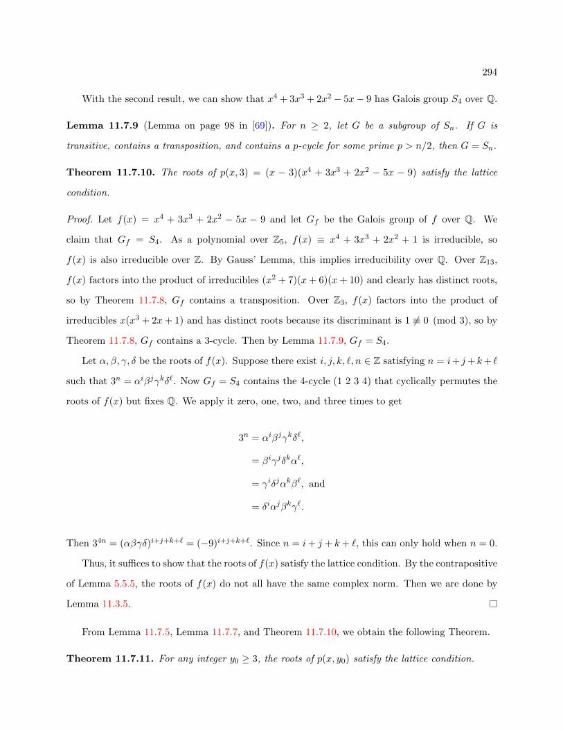
294

With the second result, we can show that x4 + 3x3 + 2x2 − 5x− 9 has Galois group S4 over Q.

Lemma 11.7.9 (Lemma on page 98 in [69]). For n ≥ 2, let G be a subgroup of Sn. If G is

transitive, contains a transposition, and contains a p-cycle for some prime p > n/2, then G = Sn.

Theorem 11.7.10. The roots of p(x, 3) = (x − 3)(x4 + 3x3 + 2x2 − 5x − 9) satisfy the lattice

condition.

Proof. Let f(x) = x4 + 3x3 + 2x2 − 5x − 9 and let Gf be the Galois group of f over Q. We

claim that Gf = S4. As a polynomial over Z5, f(x) ≡ x4 + 3x3 + 2x2 + 1 is irreducible, so

f(x) is also irreducible over Z. By Gauss’ Lemma, this implies irreducibility over Q. Over Z13,

f(x) factors into the product of irreducibles (x2 + 7)(x+ 6)(x+ 10) and clearly has distinct roots,

so by Theorem 11.7.8, Gf contains a transposition. Over Z3, f(x) factors into the product of

irreducibles x(x3 + 2x+ 1) and has distinct roots because its discriminant is 1 6≡ 0 (mod 3), so by

Theorem 11.7.8, Gf contains a 3-cycle. Then by Lemma 11.7.9, Gf = S4.

Let α, β, γ, δ be the roots of f(x). Suppose there exist i, j, k, `, n ∈ Z satisfying n = i+ j+k+ `

such that 3n = αiβjγkδ`. Now Gf = S4 contains the 4-cycle (1 2 3 4) that cyclically permutes the

roots of f(x) but fixes Q. We apply it zero, one, two, and three times to get

3n = αiβjγkδ`,

= βiγjδkα`,

= γiδjαkβ`, and

= δiαjβkγ`.

Then 34n = (αβγδ)i+j+k+` = (−9)i+j+k+`. Since n = i+ j + k+ `, this can only hold when n = 0.

Thus, it suffices to show that the roots of f(x) satisfy the lattice condition. By the contrapositive

of Lemma 5.5.5, the roots of f(x) do not all have the same complex norm. Then we are done by

Lemma 11.3.5.

From Lemma 11.7.5, Lemma 11.7.7, and Theorem 11.7.10, we obtain the following Theorem.

Theorem 11.7.11. For any integer y0 ≥ 3, the roots of p(x, y0) satisfy the lattice condition.

295

Figure 11.10: Quaternary gadget used in the interpolation construction below. Allvertices are assigned 〈3(κ− 1), κ− 3,−3〉.

We use Theorem 11.7.11 to prove Lemma 11.7.12.

Lemma 11.7.12. Suppose κ ≥ 4 is the domain size. Then Pl-Holantκ(〈3(κ − 1), κ − 3,−3〉) is

#P-hard.

Proof. Let 〈2, 0, 1, 0, 0, 0, 1, 0, 0〉 be a succinct quaternary signature of type τ4. We reduce from

Pl-Holantκ(〈2, 0, 1, 0, 0, 0, 1, 0, 0〉), which is #P-hard by Corollary 11.5.2.

Consider the gadget in Figure 11.10. We assign 〈3(κ − 1), κ − 3,−3〉 to the vertices. By

Lemma 9.2.3, the signature of this gadget is f = 〈f 1 11 1, f 1 2

1 1, f 1 2

1 2, f 1 3

1 2, f 1 2

2 1, f 1 3

2 1, f 1 1

2 2, f 1 1

2 3, f 1 4

2 3〉 up

to a nonzero factor of κ, where

f 1 11 1

= (κ− 1)(κ+ 3),

f 1 21 1

= κ− 3,

f 1 21 2

= 2κ− 3,

f 1 31 2

= κ− 3,

f 1 22 1

= 2κ− 3,

f 1 32 1

= κ− 3,

f 1 12 2

= (κ− 3)(κ+ 1),

f 1 12 3

= κ− 3, and

f 1 42 3

= −3.

Now consider the recursive construction in Figure 11.11. We assign f to every vertex. Up to a

nonzero factor of κs, let gs be the succinct signature of type τ4 for the sth gadget in this construction.

Then g0 = 〈1, 0, 0, 0, 0, 0, 1, 0, 0〉 and gs = M sg0, where M is the matrix in Table 11.3.

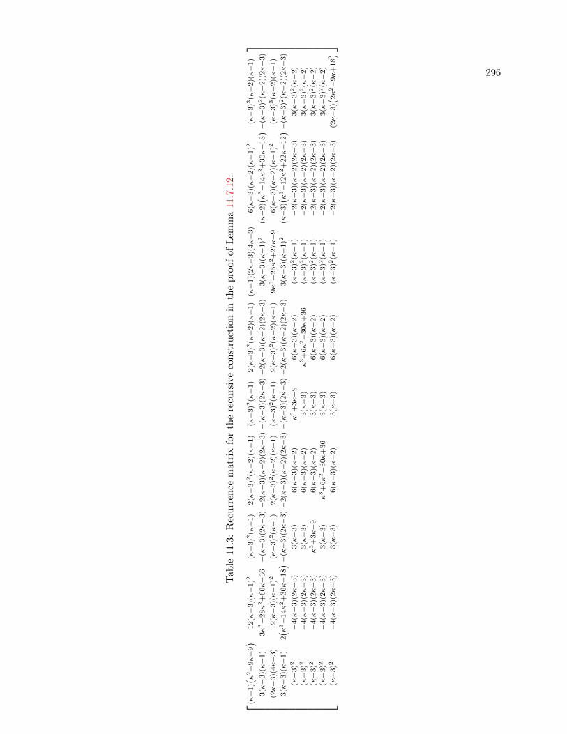
296

Tab

le11

.3:

Rec

urr

ence

mat

rix

for

the

recu

rsiv

eco

nst

ruct

ion

inth

ep

roof

ofL

emm

a11

.7.1

2.

(κ−

1) (κ2+

9κ−

9)

12(κ−

3)(κ−

1)2

(κ−

3)2

(κ−

1)

2(κ−

3)2

(κ−

2)(κ−

1)

(κ−

3)2

(κ−

1)

2(κ−

3)2

(κ−

2)(κ−

1)

(κ−

1)(

2κ−

3)(

4κ−

3)

6(κ−

3)(κ−

2)(κ−

1)2

(κ−

3)3

(κ−

2)(κ−

1)

3(κ−

3)(κ−

1)

3κ3−

28κ2+

60κ−

36−

(κ−

3)(

2κ−

3)−

2(κ−

3)(κ−

2)(

2κ−

3)−

(κ−

3)(

2κ−

3)−

2(κ−

3)(κ−

2)(

2κ−

3)

3(κ−

3)(κ−

1)2

(κ−

2) (κ3−

14κ2+

30κ−

18)−

(κ−

3)2

(κ−

2)(

2κ−

3)

(2κ−

3)(

4κ−

3)

12(κ−

3)(κ−

1)2

(κ−

3)2

(κ−

1)

2(κ−

3)2

(κ−

2)(κ−

1)

(κ−

3)2

(κ−

1)

2(κ−

3)2

(κ−

2)(κ−

1)

9κ3−

26κ2+

27κ−

96(κ−

3)(κ−

2)(κ−

1)2

(κ−

3)3

(κ−

2)(κ−

1)

3(κ−

3)(κ−

1)

2(κ

3−

14κ2+

30κ−

18)−

(κ−

3)(

2κ−

3)−

2(κ−

3)(κ−

2)(

2κ−

3)−

(κ−

3)(

2κ−

3)−

2(κ−

3)(κ−

2)(

2κ−

3)

3(κ−

3)(κ−

1)2

(κ−

3) (κ3−

12κ2+

22κ−

12)−

(κ−

3)2

(κ−

2)(

2κ−

3)

(κ−

3)2

−4(κ−

3)(

2κ−

3)

3(κ−

3)

6(κ−

3)(κ−

2)

κ3+

3κ−

96(κ−

3)(κ−

2)

(κ−

3)2

(κ−

1)

−2(κ−

3)(κ−

2)(

2κ−

3)

3(κ−

3)2

(κ−

2)

(κ−

3)2

−4(κ−

3)(

2κ−

3)

3(κ−

3)

6(κ−

3)(κ−

2)

3(κ−

3)

κ3+

6κ2−

30κ

+36

(κ−

3)2

(κ−

1)

−2(κ−

3)(κ−

2)(

2κ−

3)

3(κ−

3)2

(κ−

2)

(κ−

3)2

−4(κ−

3)(

2κ−

3)

κ3+

3κ−

96(κ−

3)(κ−

2)

3(κ−

3)

6(κ−

3)(κ−

2)

(κ−

3)2

(κ−

1)

−2(κ−

3)(κ−

2)(

2κ−

3)

3(κ−

3)2

(κ−

2)

(κ−

3)2

−4(κ−

3)(

2κ−

3)

3(κ−

3)

κ3+

6κ2−

30κ

+36

3(κ−

3)

6(κ−

3)(κ−

2)

(κ−

3)2

(κ−

1)

−2(κ−

3)(κ−

2)(

2κ−

3)

3(κ−

3)2

(κ−

2)

(κ−

3)2

−4(κ−

3)(

2κ−

3)

3(κ−

3)

6(κ−

3)(κ−

2)

3(κ−

3)

6(κ−

3)(κ−

2)

(κ−

3)2

(κ−

1)

−2(κ−

3)(κ−

2)(

2κ−

3)

(2κ−

3) (

2κ2−

9κ

+18)

297

N0

Ns

Ns+1

Figure 11.11: Recursive construction to interpolate the weighted Eulerian partitionsignature. The vertices are assigned the signature of the gadget in Figure 11.10.

The row vectors

(0, 0, 0, 0,−1, 0, 0, 0, 1),

(0,−1, 0, 1,−1, 0, 0, 1, 0),

(−1, 0, 1, 0,−1, 0, 1, 0, 0), and

(0, 0, 0, 0,−1, 1, 0, 0, 0)

are linearly independent row eigenvectors of M , all with eigenvalue κ3, that are orthogonal to the

initial signature g0. Note that our target signature 〈2, 0, 1, 0, 0, 0, 1, 0, 0〉 is also orthogonal to these

four row eigenvectors.

Up to a factor of (x− κ3)4, the characteristic polynomial of M is

h(x, κ) = x5 − κ6(2κ− 1)x3 − κ9(κ2 − 2κ+ 3)x2 + (κ− 2)(κ− 1)κ12x+ (κ− 1)3κ15.

Since h(κ3, κ) = (κ− 3)κ17 and κ ≥ 4, we know that κ3 is not a root of h(x, κ) as a polynomial in

x. Thus, none of the remaining eigenvalues are κ3. The roots of h(x, κ) satisfy the lattice condition

iff the roots of

h(x, κ) =1

κ15h(κ3x, κ) = x5 − (2κ− 1)x3 − (κ2 − 2κ+ 3)x2 + (κ− 2)(κ− 1)x+ (κ− 1)3

satisfy the lattice condition. In h(x, κ), we replace κ by y + 1 to get p(x, y) = x5 − (2y + 1)x3 −

298

Figure 11.12: Square gadget used to construct the weighted Eulerian partition signa-ture.

(y2 + 2)x2 + (y− 1)yx+ y3. By Theorem 11.7.11, the roots p(x, y0) satisfy the lattice condition for

any integer y0 ≥ 3. Thus, the roots of h(x, κ) satisfy the lattice for any κ ≥ 4. In particular, this

means that the five eigenvalues of M different from κ3 are distinct, so M is diagonalizable.

The 5-by-5 matrix in the upper-left corner of [g0 Mg0 . . . M8g0] is

1 9(κ−1)2κ (κ−1)κ4(κ3−3κ2+11κ+3) (κ−1)κ7(κ3+12κ2−11κ+6) (κ−1)κ10(κ4+4κ3−4κ2+44κ−33)0 3(κ−3)(κ−1)κ −(κ−3)κ4(κ2−2κ−1) (κ−3)κ7(3κ2−3κ+2) (κ−3)κ10(κ3−4κ2+16κ−11)0 9(κ−1)2κ κ4(κ4−4κ3+6κ2+4κ−3) κ7(15κ3−28κ2+11κ−6) κ10(κ5+3κ4−22κ3+72κ2−83κ+33)0 3(κ−3)(κ−1)κ −(κ−3)(κ−1)κ4(κ+1) 2(κ−3)κ7(2κ2−κ+1) (κ−3)(κ−1)κ10(κ2−6κ+11)0 (κ−3)2κ (κ−3)κ4(κ+1) (κ−3)κ7(κ2−κ+2) (κ−3)κ10(κ3−2κ2+10κ−11)

.

Its determinant is (κ − 3)3(κ − 1)2κ26(κ4 + κ3 + 17κ2 + 3κ + 2), which is nonzero since κ ≥ 4.

Thus [g0 Mg0 . . . M8g0] has rank at least 5, so by Lemma 11.3.2, g0 is not orthogonal to the five

remaining row eigenvectors of M .

Therefore, by Lemma 11.3.6, we can interpolate 〈2, 0, 1, 0, 0, 0, 1, 0, 0〉, so we are done.

When κ = 3, 〈3(κ−1), κ−3,−3〉 simplifies to −3〈−2, 0, 1〉. We have a much simpler proof that

this signature is #P-hard.

Lemma 11.7.13. Suppose the domain size is 3. Then Pl-Holant3(〈−2, 0, 1〉) is #P-hard.

Proof. Let g = 〈2, 0, 1, 0, 0, 0, 1, 0〉 be a succinct quaternary signature of type τ4. We reduce from

Pl-Holant3(g), which is #P-hard by Corollary 11.5.2.

Consider the gadget in Figure 11.12. The vertices are assigned 〈−2, 0, 1〉. Up to a factor of 9,

the signature of this gadget is g, as desired.

We summarize this section with the following result. With all succinct binary signatures of type

τ2 available as well as the succinct unary signature 〈1〉 of type τ1, any succinct ternary signature

〈a, b, c〉 of type τ3 satisfying B 6= 0 is #P-hard.

299

Lemma 11.7.14. Suppose κ ≥ 3 is the domain size and a, b, c ∈ C. Let F be a signature set

containing the succinct ternary signature 〈a, b, c〉 of type τ3, the succinct unary signature 〈1〉 of

type τ1, and the succinct binary signature 〈x, y〉 of type τ2 for all x, y ∈ C. If B 6= 0, then

Pl-Holantκ(F) is #P-hard.

Proof. Suppose A 6= 0. By Lemma 11.7.1, we have a succinct ternary signature 〈a′, b′, b′〉 of type

τ3 with a′ 6= b′. Then we are done by Corollary 10.3.7.

Otherwise, A = 0. Since B 6= 0, we have b 6= c. By Lemma 11.7.3, we have the signature

〈3(κ− 1), κ− 3,−3〉. If κ ≥ 4, then we are done by Lemma 11.7.12. Otherwise, κ = 3 and we are

done by Lemma 11.7.13.

11.8 Main Result

Now we can prove our main dichotomy theorem.

Theorem 11.8.1. Suppose κ ≥ 3 is the domain size and a, b, c ∈ C. Let 〈a, b, c〉 be a succinct

ternary signature of type τ3. Then Pl-Holantk appa(〈a, b, c〉) is #P-hard unless at least one of the

following holds:

1. a = b = c;

2. a = c and κ = 3;

there exists λ ∈ C and T ∈ Iκ, κIκ − 2Jκ such that

3. 〈a, b, c〉 = T⊗3λ〈1, 0, 0〉;

4. 〈a, b, c〉 = T⊗3λ〈1, 0, ω〉 and κ = 3 where ω3 = 1;

5. 〈a, b, c〉 = T⊗3λ〈µ2, 1, µ〉 and κ = 4 where µ = −1± 2i;

in which case, the computation can be done in polynomial time.

Proof. The signature in case 1 is degenerate, which is trivially tractable. Case 2 is tractable by case 3

of Corollary 11.1.3. Case 3 is tractable by Corollary 11.1.4. Case 4 is tractable by Corollary 11.1.5.

Case 5 is tractable by Lemma 11.1.6.

Otherwise, 〈a, b, c〉 is none of these tractable cases. If B = 0, then we are done by Corol-

lary 11.5.5, so assume that B 6= 0. If a + (κ − 1)b = 0 and b2 − 4bc − (κ − 3)c2 = 0, then we are

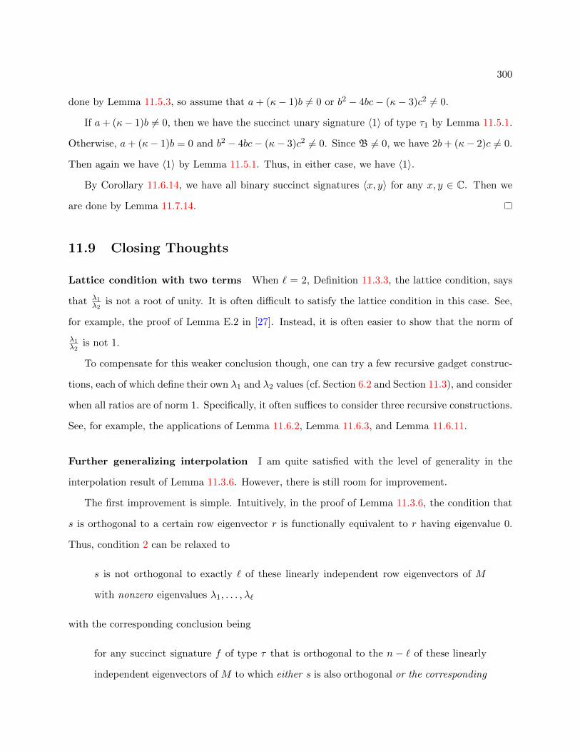
300

done by Lemma 11.5.3, so assume that a+ (κ− 1)b 6= 0 or b2 − 4bc− (κ− 3)c2 6= 0.

If a+ (κ− 1)b 6= 0, then we have the succinct unary signature 〈1〉 of type τ1 by Lemma 11.5.1.

Otherwise, a+ (κ− 1)b = 0 and b2 − 4bc− (κ− 3)c2 6= 0. Since B 6= 0, we have 2b+ (κ− 2)c 6= 0.

Then again we have 〈1〉 by Lemma 11.5.1. Thus, in either case, we have 〈1〉.

By Corollary 11.6.14, we have all binary succinct signatures 〈x, y〉 for any x, y ∈ C. Then we

are done by Lemma 11.7.14.

11.9 Closing Thoughts

Lattice condition with two terms When ` = 2, Definition 11.3.3, the lattice condition, says

that λ1λ2

is not a root of unity. It is often difficult to satisfy the lattice condition in this case. See,

for example, the proof of Lemma E.2 in [27]. Instead, it is often easier to show that the norm of

λ1λ2

is not 1.

To compensate for this weaker conclusion though, one can try a few recursive gadget construc-

tions, each of which define their own λ1 and λ2 values (cf. Section 6.2 and Section 11.3), and consider

when all ratios are of norm 1. Specifically, it often suffices to consider three recursive constructions.

See, for example, the applications of Lemma 11.6.2, Lemma 11.6.3, and Lemma 11.6.11.

Further generalizing interpolation I am quite satisfied with the level of generality in the

interpolation result of Lemma 11.3.6. However, there is still room for improvement.

The first improvement is simple. Intuitively, in the proof of Lemma 11.3.6, the condition that

s is orthogonal to a certain row eigenvector r is functionally equivalent to r having eigenvalue 0.

Thus, condition 2 can be relaxed to

s is not orthogonal to exactly ` of these linearly independent row eigenvectors of M

with nonzero eigenvalues λ1, . . . , λ`

with the corresponding conclusion being

for any succinct signature f of type τ that is orthogonal to the n − ` of these linearly

independent eigenvectors of M to which either s is also orthogonal or the corresponding

301

eigenvalue is 0.

Note that the changes here are only the addition of text, which have been emphasized.

The second improvement is more complicated. For simplicity, consider the case where s is

orthogonal to every row eigenvector. Then the three conditions imply that all eigenvalues are

distinct. However, this is not necessary. If some eigenvalues are the same, then the same conclusion

might hold if their eigenvectors are linearly dependent (i.e. the eigenvalues are in the same Jordan

block). For example, see Section 6.2, especially Lemma 6.2.4 and the paragraph that precedes it.

I am not sure what the proper generalization should be; I leave this as an open problem.

Even with these generalizations in mind, I consider Lemma 11.3.6 to be sufficiently strong for

now. Instead, I believe that an important tool for future progress on the complexity of Holant

problems will be new ways to satisfy condition 3, the lattice condition. The proof of Lemma E.2

in [27] is already one such example.

Computing Puiseux series The proof of Lemma 11.7.6 used (truncations of) the Puiseux series

y1(x) = x2 + 2x−1 + 2x−2 − 6x−4 − 18x−5 +O(x−6) for x ∈ R,

y2(x) = x3/2 − 1

2x+

1

8x1/2 − 65

128x−1/2 − x−1 − 1471

1024x−3/2 − x−2 +O(x−5/2) for x > 0, and

y3(x) = −x3/2 − 1

2x− 1

8x1/2 +

65

128x−1/2 − x−1 +

1471

1024x−3/2 − x−2 +O(x−5/2) for x > 0.

for

p(x, y) = x5 − 2x3y − x3 − x2y2 − 2x2 + xy2 − xy + y3.

Mathematica can compute these (using Series), but let me explain how one can do this by hand.

We want to understand the roots of p(x, y) for large x and y. Since series expansions are simplest

when done at 0 (or (0, 0) in this case), we invert x and y and clear denominators to get

q(x, y) = x5y3p(x−1, y−1) = x5 − x4y2 + x4y − 2x3y3 − x3y − x2y3 − 2x2y2 + y3.

To obtain our initial approximation for each root, we use Newton’s polygon. My understanding

302

0 1 2 3 4 50

1

2

3

α

β

Figure 11.13: Carrier and Newton polygon of q.

for how to do this comes from [11, Section 8.3]. Let f be a polynomial in x and y. The carrier of

f , denoted by ∆(f), is the set of pairs of exponents (α, β) for its monomials cα,βxαyβ with nonzero

coefficients (i.e. cα,β 6= 0). Then the Newton polygon of f is the convex hull of ∆(f).

The carrier of q is

∆(q) = (5, 0), (4, 2), (4, 1), (3, 3), (3, 1), (2, 3), (2, 2), (0, 3),

which is plotted in Figure 11.13 along with the Newton polygon of q. We use the lower envelope

to obtain the initial approximations.1 The lower envelope is comprised of the line segment from

(0, 3) to (3, 1) and the line segment from (3, 1) to (5, 0). The slope of the first line segment is −23 ,

which says that an initial approximation for a root is y = tx3/2 for some t ∈ C. We solve for t by

summing the monomials involved in this line segment and setting them equal to 0. In this case, we

get

y3 − x3y = (tx3/2)3 − x3(tx3/2) = tx9/2(t2 − 1) = 0,

for which the nonzero solutions are t = ±1. Therefore, initial approximations for two roots are

y = ±x3/2. The slope of the second line segment is −12 , which says that an initial approximation a

1Alternatively, we could have used the upper envelope for the Newton polygon of p.

303

root is y = tx2 for some t ∈ C. Then

x5 − x3y = x5 − x3(tx2) = x5(t− 1) = 0,

for which the only solution is t = 1. Therefore, a third initial approximation for a root is y = x2.

Now we improve each approximation using Newton’s method. For this setting with two vari-

ables, Newton’s method takes an initial approximation yold(x) and obtains a better approximation

ynew(x) according to the equation

ynew(x) = yold(x)− p(x, yold(x))

∂yp(x, yold(x)).

Since the numerator and denominator in the fraction are polynomials2 in x, we do not expect

to have cancellations in the fraction. However, we are only looking for an approximation, so we

can ignore all terms of lower order in the denominator so that the fraction can be expressed with

denominator 1. Using the initial approximation yold(x) = x2 gives

ynew(x) = yold(x)− p(x, yold(x))

∂yp(x, yold(x))

= yold(x)− x5 − 2x3yold(x)− x3 − x2yold(x)2 − 2x2 + xyold(x)2 − xyold(x) + yold(x)3

−2x3 − 2x2yold(x) + 2xyold(x)− x+ 3yold(x)2

= x2 − −2x3 − 2x2

x4 − x

≈ x2 + 2x−1 + 2x−2.

Our initial approximation was the first term of y1(x), and now we have the first three terms of

y1(x). We knew that we would get the second term from this application of Newton’s method, but

I would say that we were lucky by also getting the third term. This does not happen in general.

For example, applying Newton’s method starting with yold(x) = x2 + 2x−1 (and ignoring terms of

lower order in the denominator) gives

ynew(x) ≈ x2 + 2x−1 + 2x−2 − 6x−4 − 4x−5 − 8x−7,

2Actually, Laurent polynomials in x1/n for some positive integer n.

304

but the correct coefficient of x−5 is 18 (and the coefficients for x−6 and x−7 are also incorrect). To

be certain about each term in the new approximation, I prefer to ignore terms of lower order in

the numerator of the fraction as well. Throwing away this information will drastically slow down

the convergence rate of Newton’s method, but I only want to compute the first few terms, so this

is not a problem.

305

Chapter 12

Conclusion

This dissertation contains dichotomy theorems for several classes of Holant problems, but the com-

plexity remains unknown for many counting problems. One way to make fundamental progress

would be to obtain a better understanding of which points satisfy the lattice condition (Defini-

tion 11.3.3). For example, it is extremely easy to apply Lemma 11.3.4. Is there a similarly useful

characterization of the irreducible quartic polynomials with rational coefficients?

12.1 Future Progress on the Complexity of Holant Problems

The most pertinent question about the complexity of Holant problems involves asymmetric signa-

tures. Symmetric signatures have many nice properties, but they lack the property of being closed

under gadget constructions. Thus far, the majority of progress on Holant problems with symmetric

signatures has managed to avoid addressing the complexity of Holant problems with asymmetric

signatures.1

It is natural to consider Holant problems over regular graphs (by, for example, considering a

Holant problem in which only a single signature is available). The existing proof techniques also

work quite well for planar graphs. (Intuitively, the reason for this is that the simplest gadget

constructions are often the most useful in proving the hardness of a dichotomy theorem, and simple

gadgets are usually planar.) In contrast, little is known about the complexity of bipartite Holant

1A notable exception is Lemma 6.5.2.

306

problems (since simple gadgets are usually not bipartite).

A tough road lies ahead for anyone who considers Holant problems over higher domain sizes

(than the Boolean domain). The success we had in Chapter 10 and Chapter 11 with higher domain

Holant problems can be partially attributed to the fact that we considered a single signature with

higher degree of symmetry. Here are two specific difficulties. First, it might be that a higher

domain Holant problem is properly viewed as a Holant problem with a smaller domain size via a

holographic transformation. See the proof of Lemma 11.5.4 for an example of this. Second, higher

domain signatures can express tractable signatures that are a sum of tractable signatures. The

proof of Corollary 11.5.5 contains a simple example of this. In special cases, this can also happen

via a sum of (two) tractable signatures defined over disjoint domain elements. I also expect there

to be further difficulties that we have yet to encounter.

12.2 Future Progress on the Complexity of Graph Polynomials

One way I envision progress being made on the complexity of Holant problems is through progress

on the complexity of evaluating related graph polynomials. Chief among them is the transition

polynomial [85] (for 4-regular graphs) and its generalizations [65, 63] (to Eulerian graphs and all

graphs respectively). In particular, Lemma 10.2.2 has been partially generalized by Theorem 4.2

in [62]. Specifically, this result can be used to show (with a proof similar to that of Lemma 10.2.5)

that the transition polynomial has a significant overlap with Holant problems. By extending these

results to the two generalizations of the transition polynomial, one would find that the overlap with

Holant problems increases all the more.

There are a handful of results about the complexity of evaluating graph polynomials. I conclude

by listing in Table 12.1 all such results of which I am aware.

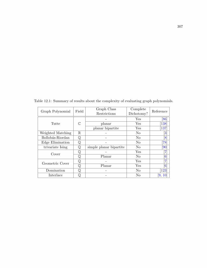
307

Table 12.1: Summary of results about the complexity of evaluating graph polynomials.

Graph Polynomial FieldGraph Class Complete

ReferenceRestrictions Dichotomy?

Tutte C- Yes [86]

planar Yes [138]planar bipartite Yes [137]

Weighted Matching R - No [3]

Bollobas-Riordan Q - No [8]

Edge Elimination Q - No [78]

trivariate Ising Q simple planar bipartite No [90]

CoverQ - Yes [7]Q Planar No [6]

Geometric CoverQ - Yes [7]Q Planar Yes [6]

Domination Q - No [123]

Interlace Q - No [9, 10]

308

Bibliography

[1] Richard Arratia, Bela Bollobas, and Gregory B. Sorkin. The interlace polynomial: A new

graph polynomial. In SODA, pages 237–245. Society for Industrial and Applied Mathematics,

2000.

[2] J. Ashkin and E. Teller. Statistics of two-dimensional lattices with four components. Phys.

Rev., 64(5-6):178–184, 1943.

[3] Ilia Averbouch and J.A.Makowsky. The complexity of multivariate matching polynomials.

http://www.cs.technion.ac.il/admlogic/TR/2007/wg07.pdf, 2007.

[4] Regis Barbanchon. On unique graph 3-colorability and parsimonious reductions in the plane.

Theor. Comput. Sci., 319(1-3):455–482, 2004.

[5] Rodney J. Baxter. Exactly solved models in statistical mechanics. Academic press London,

1982.

[6] Markus Blaser and Radu Curticapean. The complexity of the cover polynomials for planar

graphs of bounded degree. In MFCS, pages 96–107. Springer Berlin Heidelberg, 2011.

[7] Markus Blaser, Holger Dell, and Mahmoud Fouz. Complexity and approximability of the

cover polynomial. Comput. Complex., 21(3):359–419, 2012.

[8] Markus Blaser, Holger Dell, and Johann A. Makowsky. Complexity of the bollobsriordan

polynomial. exceptional points and uniform reductions. Theor. Comput. Syst., 46(4):690–

706, 2010.

309

[9] Markus Blaser and Christian Hoffmann. On the complexity of the interlace polynomial.

CoRR, abs/0707.4565, 2007.

[10] Markus Blaser and Christian Hoffmann. On the complexity of the interlace polynomial. In

STACS, pages 97–108. Schloss Dagstuhl–Leibniz-Zentrum fuer Informatik, 2008.

[11] Egbert Brieskorn and Horst Knorrer. Plane Algebraic Curves. Modern Birkhauser Classics.

Springer Basel, 1986. Translated by John Stillwell.

[12] Thomas Brylawski and James Oxley. The Tutte polynomial and its applications. In Neil

White, editor, Matriod Applications, pages 123–225. Cambridge University Press, 1992.

[13] Andrei Bulatov, Martin Dyer, Leslie Ann Goldberg, Markus Jalsenius, and David Richerby.

The complexity of weighted Boolean #CSP with mixed signs. Theor. Comput. Sci., 410(38-

40):3949–3961, 2009.

[14] Andrei Bulatov and Martin Grohe. The complexity of partition functions. Theor. Comput.

Sci., 348(2):148–186, 2005.

[15] Andrei A. Bulatov. A dichotomy theorem for constraint satisfaction problems on a 3-element

set. J. ACM, 53(1):66–120, 2006.

[16] Andrei A. Bulatov. The complexity of the counting constraint satisfaction problem. J. ACM,

60(5):34:1–34:41, 2013.

[17] Andrei A. Bulatov and Vıctor Dalmau. Towards a dichotomy theorem for the counting

constraint satisfaction problem. Inform. and Comput., 205(5):651–678, 2007.

[18] Robert Burton and Jeffrey E. Steif. Non-uniqueness of measures of maximal entropy for

subshifts of finite type. Ergodic Theory Dyn. Syst., 14(2):213–235, 1994.

[19] Robert Burton and Jeffrey E. Steif. New results on measures of maximal entropy. Israel J.

Math., 89(1-3):275–300, 1995.

[20] Jin-Yi Cai and Xi Chen. Complexity of counting CSP with complex weights. In STOC, pages

909–920. ACM, 2012.

310

[21] Jin-Yi Cai, Xi Chen, Richard J. Lipton, and Pinyan Lu. On tractable exponential sums. In

FAW, pages 148–159. Springer Berlin Heidelberg, 2010. CoRR, abs/1307.7430, 2010.

[22] Jin-Yi Cai, Xi Chen, and Pinyan Lu. Non-negatively weighted #CSP: An effective complexity

dichotomy. In CCC, pages 45–54. IEEE Computer Society, 2011.

[23] Jin-Yi Cai, Xi Chen, and Pinyan Lu. Graph homomorphisms with complex values: A di-

chotomy theorem. SIAM J. Comput., 42(3):924–1029, 2013.

[24] Jin-Yi Cai and Vinay Choudhary. Some results on matchgates and holographic algorithms.

Int. J. Software and Informatics, 1(1):3–36, 2007.

[25] Jin-Yi Cai and Vinay Choudhary. Valiant’s Holant theorem and matchgate tensors. Theor.

Comput. Sci., 384(1):22–32, 2007.

[26] Jin-Yi Cai, Vinay Choudhary, and Pinyan Lu. On the theory of matchgate computations.

Theory Comput. Syst., 45(1):108–132, 2009.

[27] Jin-Yi Cai, Zhiguo Fu, Heng Guo, and Tyson Williams. A holant dichotomy: Is the FKT

algorithm universal? In submission, 2015.

[28] Jin-Yi Cai and Aaron Gorenstein. Matchgates revisited. Theory Comput., 10(7):167–197,

2014.

[29] Jin-Yi Cai, Heng Guo, and Tyson Williams. A complete dichotomy rises from the capture of

vanishing signatures. CoRR, abs/1204.6445, 2012.

[30] Jin-Yi Cai, Heng Guo, and Tyson Williams. A complete dichotomy rises from the capture of

vanishing signatures (extended abstract). In STOC, pages 635–644. ACM, 2013.

[31] Jin-Yi Cai, Heng Guo, and Tyson Williams. Holographic algorithms beyond matchgates.

CoRR, abs/1307.7430, 2013.

[32] Jin-Yi Cai, Heng Guo, and Tyson Williams. The complexity of counting edge colorings and

a dichotomy for some higher domain Holant problems. CoRR, abs/1404.4020, 2014.

311

[33] Jin-Yi Cai, Heng Guo, and Tyson Williams. The complexity of counting edge colorings and

a dichotomy for some higher domain Holant problems (extended abstract). In FOCS, pages

601–610. IEEE, 2014.

[34] Jin-Yi Cai, Heng Guo, and Tyson Williams. Holographic algorithms beyond matchgates. In

ICALP, pages 271–282. Springer Berlin Heidelberg, 2014.

[35] Jin-Yi Cai, Sangxia Huang, and Pinyan Lu. From Holant to #CSP and back: Dichotomy for

Holantc problems. Algorithmica, 64(3):511–533, 2012.

[36] Jin-Yi Cai and Michael Kowalczyk. Spin systems on k-regular graphs with complex edge

functions. Theor. Comput. Sci., 461:2–16, 2012.

[37] Jin-Yi Cai and Michael Kowalczyk. Partition functions on k-regular graphs with 0, 1-vertex

assignments and real edge functions. Theor. Comput. Sci., 494(0):63–74, 2013.

[38] Jin-Yi Cai, Michael Kowalczyk, and Tyson Williams. Gadgets and anti-gadgets leading to a

complexity dichotomy. CoRR, abs/1108.3383, 2011.

[39] Jin-Yi Cai, Michael Kowalczyk, and Tyson Williams. Gadgets and anti-gadgets leading to a

complexity dichotomy. In ITCS, pages 452–467. ACM, 2012.

[40] Jin-Yi Cai and Pinyan Lu. On block-wise symmetric signatures for matchgates. In FCT,

pages 187–198. Springer Berlin Heidelberg, 2007.

[41] Jin-Yi Cai and Pinyan Lu. Holographic algorithms with unsymmetric signatures. In SODA,

pages 54–63. Society for Industrial and Applied Mathematics, 2008.

[42] Jin-Yi Cai and Pinyan Lu. On symmetric signatures in holographic algorithms. Theory

Comput. Syst., 46(3):398–415, 2010.

[43] Jin-Yi Cai and Pinyan Lu. Holographic algorithms: From art to science. J. Comput. Syst.

Sci., 77(1):41–61, 2011.

[44] Jin-Yi Cai and Pinyan Lu. Signature theory in holographic algorithms. Algorithmica,

61(4):779–816, 2011.

312

[45] Jin-Yi Cai, Pinyan Lu, and Mingji Xia. Holant problems and counting CSP. In STOC, pages

715–724. ACM, 2009.

[46] Jin-Yi Cai, Pinyan Lu, and Mingji Xia. Holographic algorithms with matchgates capture

precisely tractable planar #CSP. In FOCS, pages 427–436. IEEE Computer Society, 2010.

[47] Jin-Yi Cai, Pinyan Lu, and Mingji Xia. Computational complexity of Holant problems. SIAM

J. Comput., 40(4):1101–1132, 2011.

[48] Jin-Yi Cai, Pinyan Lu, and Mingji Xia. A computational proof of complexity of some re-

stricted counting problems. Theor. Comput. Sci., 412(23):2468–2485, 2011.

[49] Jin-Yi Cai, Pinyan Lu, and Mingji Xia. Dichotomy for Holant* problems of Boolean domain.

In SODA, pages 1714–1728. SIAM, 2011.

[50] Jin-Yi Cai, Pinyan Lu, and Mingji Xia. Holographic reduction, interpolation and hardness.

Computational Complexity, 21(4):573–604, 2012.

[51] Jin-Yi Cai, Pinyan Lu, and Mingji Xia. Dichotomy for Holant* problems with domain size 3.

In SODA, pages 1278–1295. SIAM, 2013.

[52] Jin-Yi Cai, Pinyan Lu, and Mingji Xia. Holographic algorithms by Fibonacci gates. Linear

Algebra Appl., 438(2):690–707, 2013.

[53] Jin-Yi Cai, Pinyan Lu, and Mingji Xia. The complexity of complex weighted Boolean #CSP.

J. Comput. System Sci., 80(1):217–236, 2014.

[54] Matthew Cook and Jehoshua Bruck. Implementability among predicates. Caltech Paradise

ETR 067, http://www.paradise.caltech.edu/papers/etr067.pdf, 2005.

[55] Nadia Creignou, Sanjeev Khanna, and Madhu Sudan. Complexity Classifications of Boolean

Constraint Satisfaction Problems. Society for Industrial and Applied Mathematics, 2001.

[56] Radu Curticapean. Counting perfect matchings in graphs that exclude a single-crossing

minor. CoRR, abs/1406.4056, 2014.

313

[57] C. T. J. Dodson and T. Poston. Tensor Geometry, volume 130 of Graduate Texts in Mathe-

matics. Springer-Verlag, second edition, 1991.

[58] Martin Dyer, Leslie Ann Goldberg, and Mark Jerrum. The complexity of weighted Boolean

#CSP. SIAM J. Comput., 38(5):1970–1986, 2009.

[59] Martin Dyer and Catherine Greenhill. The complexity of counting graph homomorphisms.

Random Struct. Algorithms, 17(3-4):260–289, 2000.

[60] Martin Dyer and David Richerby. On the complexity of #CSP. In STOC, pages 725–734.

ACM, 2010.

[61] Jack Edmonds. Paths, trees, and flowers. Canad. J. Math., 17:449–467, 1965.

[62] J. Ellis-Monaghan and I. Moffatt. Evaluations of topological Tutte polynomials. Combin.

Probab. Comput., 24(3):556–583, 2015.

[63] Joanna A. Ellis-Monaghan. New results for the Martin polynomial. J. Comb. Theory Ser. B,

74(2):326–352, 1998.

[64] Joanna A. Ellis-Monaghan. Identities for circuit partition polynomials, with applications to

the Tutte polynomial. Adv. Appl. Math., 32(1-2):188–197, 2004.

[65] Joanna A. Ellis-Monaghan and Irasema Sarmiento. Generalized transition polynomials.

Congr. Numer., 155:57–69, 2002.

[66] Gerd Faltings. Endlichkeitssatze fur abelsche Varietaten uber Zahlkorpern. Invent. Math.,

73(3):349–366, 1983.

[67] Tomas Feder and Moshe Y. Vardi. The computational structure of monotone monadic SNP

and constraint satisfaction: A study through Datalog and group theory. SIAM J. Comput.,

28(1):57–104, 1998.

[68] Michael E. Fisher. On the dimer solution of planar ising models. J. Math. Phys., 7(10):1776–

1781, 1966.

314

[69] P. X. Gallagher. The large sieve and probabilistic Galois theory. In Proc. Symp. Pure Math.,

volume 24 of Analytic Number Theory, pages 91–101. Amer. Math. Soc., 1973.

[70] Leslie Ann Goldberg, Martin Grohe, Mark Jerrum, and Marc Thurley. A complexity di-

chotomy for partition functions with mixed signs. SIAM J. Comput., 39(7):3336–3402, 2010.

[71] Heng Guo, Sangxia Huang, Pinyan Lu, and Mingji Xia. The complexity of weighted Boolean

#CSP modulo k. In STACS, pages 249–260. Schloss Dagstuhl - Leibniz-Zentrum fuer Infor-

matik, 2011.

[72] Heng Guo, Pinyan Lu, and Leslie G. Valiant. The complexity of symmetric Boolean parity

Holant problems. SIAM J. Comput., 42(1):324–356, 2013.

[73] Heng Guo and Tyson Williams. The complexity of planar Boolean #CSP with complex

weights. CoRR, abs/1212.2284, 2012.

[74] Heng Guo and Tyson Williams. The complexity of planar Boolean #CSP with complex

weights. In ICALP, pages 516–527. Springer Berlin Heidelberg, 2013.

[75] Per Hallberg. Gibbs Measures and Phase Transitions in Potts and Beach Models. PhD

thesis, Chalmers Tekniska Hogskola, 2004. http://www.dissertations.se/dissertation/

9e3d6872b0/.

[76] Johan Hastad. Tensor rank is NP-complete. J. Algorithm., 11(4):644–654, 1990.

[77] Brian Hayes. Accidental algorithms. American Scientist, 96(1), 2008.

[78] Christian Hoffmann. A most general edge elimination polynomial - thickening of edges.

Fundam. Inform., 98(4):373–378, 2010.

[79] Ian Holyer. The NP-completeness of edge-coloring. SIAM J. Comput., 10(4):718–720, 1981.

[80] Sangxia Huang and Pinyan Lu. A dichotomy for real weighted Holant problems. In CCC,

pages 96–106. IEEE Computer Society, 2012.

315

[81] Sangxia Huang and Pinyan Lu. A dichotomy for real weighted Holant problems. Preliminary

version appeared at CCC 2012, http://www.csc.kth.se/~sangxia/papers/2012-ccc.pdf,

2013.

[82] Tamas Hubai. The chromatic polynomial. Master’s thesis, Eotvos LorAnd University, 2009.

https://www.cs.elte.hu/blobs/diplomamunkak/mat/2009/hubai_tamas.pdf.

[83] Ernst Ising. Beitrag zur theorie des ferromagnetismus. Zeitschrift fur Physik, 31(1):253–258,

1925.

[84] Nathan Jacobson. Basic Algebra I. W. H. Freeman & Co., second edition, 1985.

[85] F. Jaeger. On transition polynomials of 4-regular graphs. In Gena Hahn, Gert Sabidussi,

and Robert E. Woodrow, editors, Cycles and Rays, volume 301 of NATO ASI Series, pages

123–150. Springer Netherlands, 1990.

[86] F. Jaeger, D. L. Vertigan, and D. J. A. Welsh. On the computational complexity of the Jones

and Tutte polynomials. Math. Proc. Cambridge, 108(1):35–53, 1990.

[87] P. W. Kasteleyn. The statistics of dimers on a lattice. Physica, 27(12):1209–1225, 1961.

[88] P. W. Kasteleyn. Graph theory and crystal physics. In F. Harary, editor, Graph Theory and

Theoretical Physics, pages 43–110. Academic Press, London, 1967.

[89] P.W. Kasteleyn. Dimer statistics and phase transitions. J. Math. Phys., 4(2):287–293, 1963.

[90] Tomer Kotek. Complexity of ising polynomials. Combin. Probab. Comput., 21(5):743–772,

2012.

[91] Michael Kowalczyk. Classification of a class of counting problems using holographic reduc-

tions. In COCOON, pages 472–485. Springer, 2009.

[92] Michael Kowalczyk. Dichotomy theorems for Holant problems. PhD thesis, University of

Wisconsin—Madison, 2010. http://cs.nmu.edu/~mkowalcz/research/main.pdf.

316

[93] Michael Kowalczyk and Jin-Yi Cai. Holant problems for regular graphs with complex edge

functions. In STACS, pages 525–536. Schloss Dagstuhl - Leibniz-Zentrum fuer Informatik,

2010.

[94] Michael Kowalczyk and Jin-Yi Cai. Holant problems for regular graphs with complex edge

functions. CoRR, abs/1001.0464, 2010.

[95] J. M. Landsberg, Jason Morton, and Serguei Norine. Holographic algorithms without match-

gates. Linear Algebra Appl., 438(2):782–795, 2013.

[96] J.M. Landsberg. Tensors: Geometry and Applications, volume 128 of Graduate Studies in

Mathematics. American Mathematical Society, 2011.

[97] T. D. Lee and C. N. Yang. Statistical theory of equations of state and phase transitions. II.

Lattice gas and Ising model. Phys. Rev., 87(3):410–419, 1952.

[98] Gaetan Leurent. The On-Line Encyclopedia of Integer Sequences. https://oeis.org/

A182176, Apr 2012.

[99] Daniel Leven and Zvi Galil. NP completeness of finding the chromatic index of regular graphs.

J. Algorithm., 4(1):35–44, 1983.

[100] Aaron Levin. private communication, 2013.

[101] Elliott H. Lieb. Residual entropy of square ice. Phys. Rev., 162(1):162–172, 1967.

[102] Elliott H. Lieb and Alan D. Sokal. A general Lee-Yang theorem for one-component and

multicomponent ferromagnets. Comm. Math. Phys., 80(2):153–179, 1981.

[103] Nathan Linial. Hard enumeration problems in geometry and combinatorics. SIAM J. Alg.

Discr. Meth., 7(2):331–335, 1986.

[104] Charles H.C. Little. An extension of Kasteleyn’s method of enumerating the 1-factors of

planar graphs. In Derek A. Holton, editor, Combinatorial Mathematics, Proceedings of the

Second Australian Conference, volume 403 of Lecture Notes in Mathematics, pages 63–72.

Springer Berlin Heidelberg, 1974.

317

[105] Pierre Martin. Enumerations Euleriennes dans les multigraphes et invariants de

Tutte-Grothendieck. PhD thesis, Joseph Fourier University, 1977. http://tel.

archives-ouvertes.fr/tel-00287330.

[106] Jason Morton. Pfaffian circuits. CoRR, abs/1101.0129, 2011.

[107] Jason Morton and Susan Margulies. Polynomial-time solvable #CSP problems via algebraic

models and Pfaffian circuits. CoRR, abs/1311.4066, 2013. To appear in Journal of Symbolic

Computation.

[108] Peter Muller. Hilbert’s irreducibility theorem for prime degree and general polynomials. Israel

J. Math., 109(1):319–337, 1999.

[109] Lars Onsager. Crystal statistics. I. A two-dimensional model with an order-disorder transition.

Phys. Rev., 65(3-4):117–149, 1944.

[110] Julius Petersen. Die theorie der regularen graphs. Acta Mathematica, 15(1):193–220, 1891.

[111] Bjorn Poonen. private communication, 2013.

[112] R. B. Potts. Some generalized order-disorder transformations. Math. Proc. Cambridge,

48(1):106–109, 1952.

[113] J. Scott Provan and Michael O. Ball. The complexity of counting cuts and of computing the

probability that a graph is connected. SIAM J. Comput., 12(4):777–788, 1983.

[114] Guus Regts. Graph parameters and invariants of the orthogonal group. PhD thesis, Univer-

siteit van Amsterdam, 2013. http://dare.uva.nl/record/1/399823.

[115] Carl Ludwig Siegel. Uber einige anwendungen diophantischer approximationen. Abh. Pruess.

Akad. Wiss. Phys. Math. Kl., pages 41–69, 1929.

[116] Ian Stewart. Galois Theory. Chapman Hall/CRC Mathematics Series. Taylor & Francis,

third edition, 2003.

318

[117] Michael Stiebitz, Diego Scheide, Bjarne Toft, and Lene M. Favrholdt. Graph Edge Coloring:

Vizing’s Theorem and Goldberg’s Conjecture. Wiley, 2012.

[118] Simon Straub, Thomas Thierauf, and Fabian Wagner. Counting the number of perfect match-

ings in k5-free graphs. In CCC, pages 66–77. IEEE Computer Society, 2014.

[119] Peter Tait. Remarks on the colourings of maps. Proc. R. Soc. Edinburgh, 10:729, 1880.

[120] H. N. V. Temperley and Michael E. Fisher. Dimer problem in statistical mechanics—an exact

result. Philosophical Magazine, 6(68):1061–1063, 1961.

[121] Marc Thurley. The Complexity of Partition Functions. PhD thesis, Humboldt-Universitat zu

Berlin, 2009. https://sites.google.com/site/marcthurley/diss_thurley.pdf.

[122] Marc Thurley. The complexity of partition functions on Hermitian matrices. CoRR,

abs/1004.0992, 2010.

[123] Peter Tittmann Tomer Kotek, James Preen. Domination polynomials of graph products.

CoRR, abs/1305.1475, 2013.

[124] Salil P. Vadhan. The complexity of counting in sparse, regular, and planar graphs. SIAM J.

Comput., 31(2):398–427, 2001.

[125] Leslie G. Valiant. The complexity of computing the permanent. Theor. Comput. Sci.,

8(2):189–201, 1979.

[126] Leslie G. Valiant. The complexity of enumeration and reliability problems. SIAM J. Comput.,

8(3):410–421, 1979.

[127] Leslie G. Valiant. Expressiveness of matchgates. Theor. Comput. Sci., 289(1):457–471, 2002.

[128] Leslie G. Valiant. Quantum circuits that can be simulated classically in polynomial time.

SIAM J. Comput., 31(4):1229–1254, 2002.

[129] Leslie G. Valiant. Corrigendum to “Expressiveness of matchgates”: [Theor. Comput. Sci.

289(1) (2002) 457471]. Theor. Comput. Sci., 299(1-3):795, 2003.

319

[130] Leslie G. Valiant. Holographic circuits. In ICALP, pages 1–15. Springer Berlin Heidelberg,

2005.

[131] Leslie G. Valiant. Accidental algorthims. In FOCS, pages 509–517. IEEE Computer Society,

2006.

[132] Leslie G. Valiant. Holographic algorithms. SIAM J. Comput., 37(5):1565–1594, 2008.

[133] Leslie G. Valiant. Some observations on holographic algorithms. In LATIN, pages 577–590.

Springer Berlin Heidelberg, 2010.

[134] Vijay V. Vazirani. NC algorithms for computing the number of perfect matchings in k3,3-free

graphs and related problems. Inform. and Comput., 80(2):152–164, 1989.

[135] Michel Las Vergnas. Le polynome de Martin d’un graphe Eulerien. Ann. Discrete Math.,

17:397–411, 1983.

[136] Michel Las Vergnas. On the evaluation at (3, 3) of the Tutte polynomial of a graph. J. Comb.

Theory, Ser. B, 45(3):367–372, 1988.

[137] D. L. Vertigan and D. J. A. Welsh. The computational complexity of the Tutte plane: the

bipartite case. Combin. Probab. Comput., 1(2):181–187, 1992.

[138] Dirk Vertigan. The computational complexity of Tutte invariants for planar graphs. SIAM

J. Comput., 35(3):690–712, 2005.

[139] Vadim G. Vizing. Critical graphs with given chromatic class. Metody Diskret. Analiz., 5:9–17,

1965.

[140] P. G. Walsh. A quantitative version of Runge’s theorem on Diophantine equations. Acta

Arith., 62(2):157–172, 1992.

[141] Dominic Welsh. Complexity: Knots, Colourings and Countings. London Mathematical Soci-

ety Lecture Note Series. Cambridge University Press, 1993.

320

[142] B. Widom and J. S. Rowlinson. New model for the study of liquidvapor phase transitions.

J. Chem. Phys, 52(4):1670–1684, 1970.

[143] Mingji Xia. Holographic reduction: A domain changed application and its partial converse

theorems. Int. J. Software and Informatics, 5(4):567–577, 2011.

[144] Mingji Xia, Peng Zhang, and Wenbo Zhao. Computational complexity of counting problems

on 3-regular planar graphs. Theor. Comput. Sci., 384(1):111–125, 2007.

[145] C. N. Yang. The spontaneous magnetization of a two-dimensional Ising model. Phys. Rev.,

85(5):808–816, 1952.

[146] C. N. Yang and T. D. Lee. Statistical theory of equations of state and phase transitions. I.

Theory of condensation. Phys. Rev., 87(3):404–409, 1952.