Advances in the Modelling of Motorcycle Dynamics · ADVANCES IN THE MODELLING OF MOTORCYCLE DYNAMICS 253 Figure 1. Scaled diagrammatic motorcycle in side view. 2.2. INERTIAS AND …

Multibody System Dynamics 12: 251–283, 2004.C© 2004 Kluwer Academic Publishers. Printed in the Netherlands. 251

Advances in the Modelling of MotorcycleDynamics

R.S. SHARP, S. EVANGELOU and D.J.N. LIMEBEERElectrical and Electronic Engineering, Imperial College London, South Kensington Campus,London SW7 2AZ, UK; E-mail: [email protected]

(Received: 7 July 2003; accepted in revised form: 7 June 2004)

Abstract. Starting from an existing advanced motorcycle dynamics model, which allows simulationof reasonably general motions and stability, modal and response computations for small perturbationsfrom any trim condition, improvements are described. These concern (a) tyre/road contact geometry,(b) tyre shear force and moment descriptions, as functions of load, slip and camber, (c) tyre relax-ation properties, (d) a new analytic treatment of the monoshock rear suspension mechanism withsample results, (e) parameter values describing a contemporary high performance machine and rider,(f) steady-state equilibrium and power checking and (g) steering control. In particular, the “MagicFormula” motorcycle tyre model is utilised and complete sets of parameter values for contemporarytyres are derived by identification methods. The new model is used for steady turning, stability, designparameter sensitivity and response to road forcing calculations. The results show the predictions of themodel to be in general agreement with observations of motorcycle behaviour from the field and theysuggest that frame flexibility remains an important design and analysis area, despite improvementsin frame designs over recent years. Motorcycle rider parameters have significant influences on thebehaviour, with results consistent with a commonly held view, that lightweight riders are more likelyto suffer oscillation problems than heavyweight ones.

Keywords: motorcycle, tyre, contact, monoshock, stability, response, sensitivity.

1. Introduction

The handling qualities of motorcycles are often of great importance. They affectthe pleasure to be gained from the rider–machine interactions and the safety ofthe rider. Self-steering action is crucial with single track vehicles and rider controlis primarily by steering torque, so-called free-control [1]. A consequence of thefree steering system is that motorcycles are oscillatory. Several modes of motionpotentially have small damping factors. Therefore much attention must be directedtowards controlling the oscillatory tendencies, throughout the operating range. Also,it is desirable that motorcycles are responsive to the rider’s commands and stabilityshould not be pursued without reference to other qualities.

In straight running, motorcycles are substantially symmetric and in-plane andout-of-plane motions are decoupled at first order level [1, 2]. In cornering, in-plane and out-of-plane cross-coupling makes any effective analysis of the dynamicscomplicated. Automated multibody dynamics analysis software [3–7] has openedup the topic significantly in recent years. The steady turning problem can be solved,

252 R.S. SHARP ET AL.

possibly with the aid of a stabilising steering controller, and modal analysis can becompleted for small perturbations from any equilibrium “trim” state.

Accuracy of predicted behaviour depends, not only on effective conceptual mod-elling and multibody analysis, but also on good parameter values. Central issuesin modelling include the representations of frame flexibilities, tyre–road contactgeometry and tyre shear forces. Many previous findings relate to motorcycle andtyre descriptions which are now somewhat dated and to tyre models which havea limited domain of applicability. It is therefore of interest (i) to obtain a para-metric description of a modern machine, (ii) to utilise a more comprehensive tyreforce model, with parameter values to correspond to a modern set of tyres, (iii)to determine steady turning, stability, response and parameter sensitivity data forcomparison with older information, to determine to what extent it remains valid,and (iv) to better understand the design of modern machines. The paper is subse-quently an account of such work. Novel analysis of a “monoshock” rear suspensionsystem is also included.

2. Parametric Description of a Modern Motorcycle

The authors are currently engaged in a measurement campaign to obtain the rele-vant parameters of a Suzuki GSX-R1000K1 machine. Such a motorcycle has beendisassembled and many of its parts have been measured, starting with the lighterones. At this stage, the campaign is incomplete. In particular, the frame stiffnessand damping parameters used and the location of the elastic centre are currentlyonly estimates.

2.1. GEOMETRY AND MASSES

The workshop manual for the motorcycle includes pictures to scale and key dimen-sions, like the wheelbase and the steering head angle. Joints between componentsat the steering head and the swing arm pivot can be identified there and many keypoints, including those related to the monoshock rear suspension, can be locatedwith reasonable precision from these pictures. A scaled diagrammatic representa-tion of the motorcycle is shown in Figure 1, the corresponding parameter valuesbeing included in an Appendix. The front frame has been measured separately togive the points p3 and p5. The point p4 is along the line of the lower front forktranslation relative to the upper forks. The estimated location p2 is the elastic centreof the rear frame with respect to a moment perpendicular to the steer axis.

The rider’s total mass is taken as 72 kg, 62% of which is associated with theupper body. The masses of the hands and half of the lower arms may be consideredto be part of the steering system. The rider parameters derive from bio-mechanicaldata [8], accounting for his posture on the machine.

Circles representing the body mass centres are in proportion to the massesconcerned, which are known through straightforward weighing.

ADVANCES IN THE MODELLING OF MOTORCYCLE DYNAMICS 253

Figure 1. Scaled diagrammatic motorcycle in side view.

2.2. INERTIAS AND MASS CENTRES

Wheel and tyre inertias have been obtained by timing oscillations of bi-filar andtri-filar suspension arrangements, utilising axial symmetry in each set-up. Similarbi-filar suspension systems have been used separately for the front and rear frames(Figure 2). Each of these is assumed to have a plane of symmetry and it is clear thatthe front frame principal axes, in the plane of symmetry, are along and perpendicularto the line of the forks. Oscillation periods, geometric dimensions and the mass ofthe suspended body lead simply to the moment of inertia about the rotation axisand standard transformations allow the determination of principal inertias and axesfor the more complex rear frame [9].

Recent measurements on a driving simulator [10] provide estimates of thecontributions to the front frame inertia, steering stiffness and steering dampingthat arise from the rider’s arms and hands, corresponding to relaxed and tenseriding. These can be added to the measured values if it is considered appropri-ate [11]. The swing arm inertias are small enough to be obtained by estimationbased on the mass centre location and the dimensions. The wheels have their masscentres at their geometric centres. Other mass centre locations were found usingplumb lines and taking photographs (Figure 2). Relevant values are given in theappendix.

2.3. STIFFNESS AND DAMPING PROPERTIES

Springs and dampers were tested in a standard dynamic materials testing machine[12]. The maximum actuator velocity available was about 0.25 m/s, which con-strained the damper characteristic measurements. Uni-directional forcing of thesteering damper up to the maximum rate of the actuator yielded a substantiallylinear force/velocity relationship with slope 4340 N/(m/s). Using the effective


Figure 2. Bifilar suspended motorcycle rear frame for inertia measurement.

moment arm of the damper (0.04 m) to convert this value to an equivalent rotationalcoefficient gives a value, 6.944 Nm/(rad/s).

The dimensions of the single rear steel spring, from the monoshock suspensionwere measured and the standard helical spring formula, k = Gd4/(64R3n), wasapplied to calculating the rate, k, as 55 kN/m. The gas filled damper contributessome suspension preload and a small rate, determined from the test machine viastatic measurements as 3.57 kN/m. The damper unit was stroked at full actuator


performance first in compression and then in extension, achieving velocities up toabout 0.13 m/s. Allowing for the gas pressure forces in the processing, the dampingcoefficient in compression was 9.6 kN/(m/s) and in rebound 13.7 kN/(m/s). Frontspring and damper coefficients are estimates, at this stage. Suspension limit stops areincluded at each end, modelled as fifth powers of displacement from stop contact.The relevant displacements are known from examination of the parts and frominformation given in the workshop manual.

The torsional stiffness of the main frame, between the steering head and thepower unit, remains to be measured. It is clear from the structural design andmaterials used that the frame is considerably stiffer than was the norm for tubularframed motorcycles of some years ago. In those cases, it was established that theframe flexibility was an essential contributor to the stability of the wobble mode,in particular [13, 14]. It remains to be seen how significant this area is for modernmachines. The torsional stiffness assumed, at 105 Nm/rad, is 3.5 times that measuredstatically for a Yamaha 650S [15] and 2.9 times that measured at about the sametime by Koenen [2]. Tyre radial stiffnesses come directly from [7].

The rider’s upper body has roll freedom relative to the main frame, while thelower body is part of the main frame. The upper body is restrained by a parallelspring damper system. Stiffness and damping parameters are chosen in alignmentwith the experimental results of Nishimi et al [16], obtained by identifying “rider”parameters in forced vibration on a mock motorcycle frame. The decoupled naturalfrequency of the rider upper body in roll is 1.27 Hz and the corresponding dampingfactor is 0.489. According to this model, rider resonance will not be apparent due tothe high damping factor and it will not be tuned to the machine oscillations, wherethese are at all vigorous.

2.4. AERODYNAMICS

Aerodynamic drag, lift and pitching moment data come from a Triumph motorcycleof similar style and dimensions to the GSX-R1000 [1]. This is steady-state dragforce, lift force and pitching moment data from full scale wind tunnel testing, witha prone rider.

3. Tyre–Road Contact Modelling

The geometry of the contact between the front tyre and the ground is a relativelycomplex part of the motorcycle modelling. It is also important to the behaviour ofthe machine. It has been common to represent the tyre as a thin disc, with the contactpoint migrating circumferentially for larger camber and steer angles, but Cossalteret al have pioneered the inclusion of tyre width in their descriptions [7, 17–19].If a disc model is used, it needs to be augmented with an overturning momentdescription [2, 5]. This is not necessary with a thick tyre model, since the lateralmigration of the contact point then occurs automatically and the overturning mo-ment is a consequence of that movement. A wide tyre with a circular cross-section


Figure 3. Diagrammatic three-dimensional front wheel contact geometry.

crown is now modelled. In addition to making the overturning moment automatic,longitudinal forces applied to the cambered tyre will lead to realistic aligningmoments appearing automatically. A necessary test for the wide tyre model isthat it gives the same results as the thin tyre model, when physically equivalentsystems are being represented. This test has been applied, with some significantconsequences.

To define each tyre/ground contact point (Figures 3 and 4) the vertical and thewheel spindle directions are used in a vector (cross) product to describe the longitu-dinal direction, with respect to the wheel. Similarly, the wheel radial direction, OCin Figure 3, comes from combining the longitudinal and wheel spindle directions.The vector OC is of fixed length and so is completely specified. G is vertically belowC and the difference between the tyre crown radius and the distance CG definesthe change in the tyre carcass compression from the nominal state and hence thechange of the wheel load from the nominal, via the tyre radial stiffness. If the roadis profiled, the road height is accounted for in working out the wheel load. Thevector OG = OC + CG defines the contact point, which belongs to the wheel butmoves within it. G remains at road surface height but the tyre load cannot becomenegative. If the tyre leaves the ground, the shear forces are zero, whatever the otherconditions are. Tyre forces are applied to the point G, in each case.

The longitudinal slip is the rearward component of the material contact pointvelocity divided by the absolute value of the rolling velocity, the latter being theforward velocity of the contact point (or the crown centre point, since these arethe same). The contact point is defined by its coordinates in the parent body of thewheel and it is de-spun relative to the material contact point. Thus the longitudinal


Figure 4. Diagrammatic two-dimensional front wheel contact geometry.

slip is given by an expression of the form:

κ = −(rolling velocity + spin component of longitudinal velocity)

/abs(rolling velocity)

The slip angle is the arctangent of the ratio of the (negative) lateral velocity of thetyre contact centre point to the absolute value of the rolling velocity.

In developing this new model from the former one [5], in which the wheelswere represented as thin discs, subtle differences between the root locus predic-tions of the old and new versions were observed in circumstances which were at thatstage thought physically equivalent. Such differences were found to be associatedwith the former description of the slip angles as deriving from the lateral veloc-ity components of the disc tyre contact points. When the wheel camber angle ischanging, these points have a small lateral velocity component not connected withsideslipping, since with the real tyre, the contact point moves around the circularsection sidewall of the tyre. The former model would have provided a more accuratedescription if it had used the crown centre point velocities to derive the slip angles.

4. Tyre Forces and Moments

The basis for the new tyre modelling is the “Magic Formula” [20–22]. The originaldevelopment was for car tyres [23], in which context, it has become dominant. The


extension for motorcycle tyres is relatively recent, with substantial changes beingnecessary to accommodate the completely different roles of sideslip and camberforces in the two cases. In each case, the “Magic Formula” is a set of equationsrelating load, slip ratio (longitudinal slip), slip angle and camber angle to longitudi-nal force, sideforce and aligning moment (and possibly overturning moment), withconstraints on the parameters to prevent the behaviour from becoming unreasonablein any operating conditions. Only very limited parameter values can be found inthe literature, but a certain amount of relevant experimental data is available. Suchdata can be used for parameter identification.

A complete set of parameter values for a given tyre will allow the calculation ofthe steady-state force and moment system for any realistic operating condition. Itis required here to determine such a full set of parameters for modern front and rearhigh performance motorcycle tyres, imposing the condition that the modelled tyreshave left/right symmetry. Test data used shows bias and it is necessary to ignoresuch bias and to omit certain offset terms from the “Magic Formula” relations, inorder to model the generic, rather than the particular. Significant published datacan be found in [2, 20–25]. Naturally, the older data refers to older tyres, while thenewer data relates to contemporary ones. The main sources relied upon here are[20, 23]. The other sources are used for checking purposes, as appropriate.

4.1. LONGITUDINAL FORCES IN PURE LONGITUDINAL SLIP

From Pacejka [23], with the simplifications explained above, the “Magic Formula”expressions for the pure longitudinal slip case are:

d fz = (Fz − Fz0)/Fz0 (1)

Fx0 = Dx sin[Cx arctan{Bxκ − Ex (Bxκ − arctan(Bxκ))}] (2)

Dx = (pDx1 + pDx2d fz)Fz (3)

Ex = (pEx1 + pEx2d fz + pEx3d f 2

z

) · (1 − pEx4sgn(κ)) (4)

Kxκ = Fz(pK x1 + pK x2d fz) · exp(pK x3d fz) (5)

Bx = Kxκ/(Cx Dx ) (6)

which must satisfy the constraints Dx > 0 and Ex < 1.Corresponding test results for a 160/70 ZR17 tyre are shown in [23]. The se-

quential quadratic programming constrained optimisation routine “fmincon” wasemployed1 to iteratively improve the elements of a starting vector of parameters

1 Alternatively, for unconstrained optimization, the Nelder Mead Simplex routine “fminsearch”was employed. Also occasionally, it was necessary to “invent” data, outside the range of experimentalresults available, to force the identified parameters to give sensible predictions over a wide range ofoperating circumstances, a problem also referred to in [26]. Often, reasonably accurate starting valuesfor the parameters were needed to ensure convergence to the optimal solution. The methods need tobe judged by the results obtained.


Table I. Best-fit parameter values for longitudinal force from 160/70 tyre.

Cx pDx1 pDx2 pEx1 pEx2 pEx3 pEx4 pK x1 pK x2 pK x3

1.6064 1.2017 −0.0922 0.0263 0.27056 −0.0769 1.1268 25.94 −4.233 0.3369

Figure 5. Tyre longitudinal force results for a 160/70 tyre from [23] (thick lines) with best-fitreconstructions (thin lines).

appearing in Equations (1)–(5). The nominal normal load Fz0 was chosen to be1600 N based on typical usage of such a tyre. That choice is far from critical,in fact, a change leading to compensatory changes in other parameters. Optimalparameters are given in Table I and the fits are illustrated in Figure 5. The twoconstraints are satisfied for loads less than 20890 N, which includes all practicalcircumstances.

Longitudinal force results are not available for any other tyres, so lateral forcesare considered next.

4.2. LATERAL FORCES IN PURE SIDESLIP AND CAMBER

In exactly the same way, the relevant equations for the lateral force are:

Fy0 = Dy sin[Cy arctan{Byβ − Ey(Byβ − arctan(Byβ))}+ Cγ arctan{Bγ γ − Eγ (Bγ γ − arctan(Bγ γ ))}] (7)


Figure 6. Tyre lateral force results for a 160/70 tyre from [23] (thick lines) with best-fitreconstructions (thin lines). Camber angles 5, 0, −5, −10, −20, −30◦.

Dy = Fz pDy1 exp(pDy2d fz)/(1 + pDy3γ2) (8)

Ey = pEy1 + pEy2γ2 + pEy4γ sgn(β) (9)

Kyα = pK y1 Fz0 sin[pK y2 arctan{Fz/((pK y3 + pK y4γ2)Fz0)}]

/(1 + pK y5γ2) (10)

By = Kyα/(Cy Dy) (11)

Kyγ = (pK y6 + pK y7d fz)Fz (12)

Bγ = Kyγ /(Cγ Dy) (13)

with the constraints Cy + Cγ < 2, Cy > 0, Dy > 0, Ey < 1, Cg > 0, Eg < 1.For the same tyre as before, the parameter optimisation process, with the effectivefriction coefficient limited to values no greater than 1.3, gives the results illustratedin Figure 6 with parameter values given below in Table II. For this particular tyre,pK y7 in Equation (12) was set to zero, because experimental results are only available

Table II. Best-fit parameter values for lateral force from 160/70 (top), 120/70 (middle) and180/55 (bottom) tyres

Cy pDy1 pDy2 pDy3 pEy1 pEy2 pEy4 pK y1

0.93921 1.1524 −0.01794 −0.06531 −0.94635 −0.09845 −1.6416 26.601

0.8327 1.3 0 0 −1.2556 −3.2068 −3.998 22.841

0.9 1.3 0 0 −2.2227 −1.669 −4.288 15.791

pK y2 pK y3 pK y4 pK y5 Cγ pK y6 pK y7 Eγ

1.0167 1.4989 0.52567 −0.24064 0.50732 0.7667 0 −4.7481

2.1578 2.5058 −0.08088 −0.22882 0.86765 0.69677 −0.03077 −15.815

1.6935 1.4604 0.669 0.18708 0.61397 0.45512 0.013293 −19.99


Figure 7. Tyre lateral force results for 120/70 tyre from [20] (thick lines) with best-fit recon-structions (thin lines). Camber angles 0, 10, 20, 30, 40, 45◦.

at non-zero camber angle for one load. This is consistent with results obtained for120/70 and 180/55 tyres (see below), for which pK y7 is relatively small, beingpositive in one case and negative in the other. All the constraints are satisfied forcamber angles less than 70◦ in magnitude.

Next, the lateral force fitting is repeated for the experimental results includedin [20] for a 120/70 front tyre and a 180/55 rear tyre, first recognising that theformer results suffer from an unreasonable positive force offset, especially for thesmaller loads, which would imply a friction coefficient greater than 2, if they weretrue. To avoid responding too strongly to these apparently spurious features, Dy isallowed to be no greater than 1.3 times Fz . Also, the measurements for slip anglesgreater than +5◦ are ignored. The previous rear tyre value of Fz0 as 1600 N isretained while the non-critical value for the front tyre was chosen as 1100 N. Best-fit parameters are shown in Table II, with Figures 7 and 8 showing the quality of thefits for the front and rear tyres respectively. All the constraints are satisfied by theseparameters.


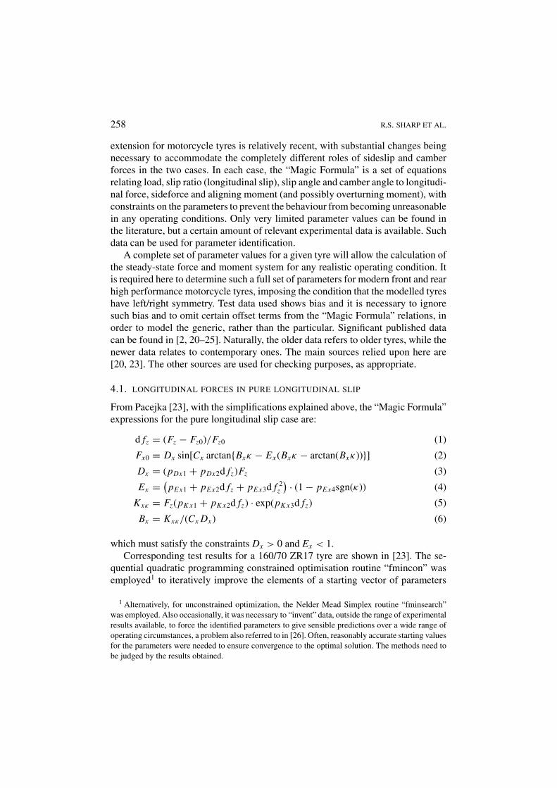
Figure 8. Tyre lateral force results for 180/55 tyre from [20] (thick lines) with best-fit recon-structions (thin lines). Camber angles 0, 10, 20, 30, 40, 45◦.

4.3. ALIGNING MOMENTS IN LATERAL SLIP AND CAMBER

Aligning moment results are included in [23] for the 160/70 tyre and in [20] for120/70 and 180/55 tyres. Three loads are covered in the former but only two inthe latter, which makes the model very heavy in parameters for the amount ofexperimental data available. In setting the parameters for the 160/70 tyre of [23]assuming the full quadratic dependency of Bt on load, the fitting is good within theload range used for the measurements but the extrapolation is poor, with constraintviolations at low and high loads. With linear dependency, the fitting is almost as goodand the extrapolation problem can be eliminated. Consequently, Bt is consideredlinear with load. Even so, there are many parameter combinations which givealmost equally good fits to the limited data. It is advantageous to use some physicalreasoning to guide the choice between the alternatives. The product of Bt , Ct andDt is the aligning moment stiffness of the tyre. According to the “Brush Model”[23], the aligning moment stiffness is proportional to load to the power 1.5, so thatfeature is used to aid the choice of the secondary parameters qBz1 and qBz2, see (18).It turns out to be quite feasible to match that characteristic closely. Also, as before,


Table III. Best-fit parameter values for aligning moment from 160/70 (top), 120/70 (middle)and 180/55 tyre (bottom)

Ct qBz1 qBz2 qBz5 qBz6 qBz9 qBz10

1.3115 10.354 4.3004 −0.34033 −0.13202 10.118 −1.0508

1.0917 10.486 −0.001154 −0.68973 1.0411 27.445 −1.0792

1.3153 10.041 −1.61e-8 −0.76784 0.73422 16.39 −0.35549

qDz1 qDz2 qDz3 qDz4 qDz8 qDz9 qDz10

0.20059 0.05282 −0.21116 −0.15941 0.30941 0 0.10037

0.19796 0.06563 0.2199 0.21866 0.3682 0.1218 0.25439

0.26331 0.030987 −0.62013 0.98524 0.50453 0.36312 −0.19168

qDz11 qEz1 qEz2 qEz5 qH z3 qH z4

0 −3.9247 10.809 0.9836 −0.04908 0

−0.17873 −0.91586 0.11625 1.4387 −0.003789 −0.01557

−0.40709 −0.19924 −0.017638 3.6511 −0.028448 −0.009862

right/left symmetry and zero offsets are assumed, making qEz4, qH z1 and qH z2 zero.The relevant “Magic Formula” Equations [23] are:

Mz0 = Mzt0 + Mzr0 (14)

Mzt0 = −Dt cos[Ct arctan{Btβ − Et (Btβ − arctan(Btβ))}]/√

1 + β2 · Fy0,γ=0 (15)

Mzr0 = Dr cos[arctan(Br (β + SHr )] (16)

SHr = (qH z3 + qH z4d fz)γ (17)

Bt = (qBz1 + qBz2d fz)(1 + qBz5|γ | + qBz6γ2) (18)

Dt = Fz(R0/Fz0)(qDz1 + qDz2d fz)(1 + qDz3|γ | + qDz4γ2) (19)

Et = (qEz1 + qEz2d fz){1 + qEz5γ (2/π ) arctan(BtCtβ)} (20)

Br = qBz9 + qBz10 ByCy (21)

Dr = Fz R0{(qDz8 + qDz9d fz)γ + (qDz10 + qDz11d fz)γ |γ |}/√

1 + β2 (22)

with the constraints: Bt > 0, Ct > 0 and Et < 1. For the 160/70 tyre, qH z4

in Equation (17) and qDz9 and qDz11 in Equation (22) are set to zero, becauseexperimental results are only provided at non-zero camber angle for one load.

The tyre crown radius, R0, for each tyre derives from the cross-sectional geome-try as 0.08 m for 160/70, 0.06 m for 120/70 and 0.09 m for 180/55 [7]. Identificationof the remaining parameters using “fmincon” as before gives the values in TableIII. Constraint violations occur only for loads greater than 11 kN, sideslip anglegreater than 45◦ or camber angle greater than 60◦. These violations are outside thepractical running range. The fit qualities are shown in Figures 9–11.


Figure 9. Tyre aligning moment results for 160/70 tyre from [23] (thick lines) with best-fitreconstructions (thin lines). Camber angles 5, 0, −5, −10, −20, −30◦.

Figure 10. Tyre aligning moment results for 120/70 tyre from [20] (thick lines) with best-fitreconstructions (thin lines). Camber angles 0, 10, 20, 30, 40, 45◦.

Figure 11. Tyre aligning moment results for 180/55 tyre from [20] (thick lines) with best-fitreconstructions (thin lines). Camber angles 0, 10, 20, 30, 40 and 45◦.


4.4. COMBINED SLIP RESULTS

4.4.1. Longitudinal Forces

In the “Magic Formula” scheme, the loss of longitudinal force due to sideslipping isdescribed by a “loss function” to be applied to the pure slip force described above.Presuming as before that the generic tyres of interest will be symmetric (SH xα = 0)and, in the absence of any indication to the contrary, assuming that wheel camberwill not affect the loss of longitudinal force due to sideslipping (rBx 3 = 0), theequations describing the loss are:

Fx = cos[Cxα arctan(Bxαβ)]Fx0 (23)

Bxα = rBx1 cos[arctan(rBx2κ)] (24)

with the constraints that Fx > 0 and Bxα > 0.The only relevant combined slip data available is from [23] for the 160/70 tyre

for 3 kN load and zero camber angle. The same parameter identification processas before yielded the best values as rBx 1 = 13.476; rBx 2 = 11.354; Cxα = 1.1231,with the fit quality shown in Figure 12. The constraint on Bxα is always satisfiedwhile that on Fx is satisfied for slip angles less than 23◦, which is considered toprovide an adequate operating range.

4.4.2. Lateral Forces

In the same way (with SV yκ = SH yκ = rBy4 = 0), the equations describing the lossof lateral force due to longitudinal slip are:

Fy = cos[Cyκ arctan(Byκκ)]Fy0 (25)

Byκ = rBy1 cos[arctan{rBy2(β − rBy3)}] (26)

with constraints Fy > 0 and Byk > 0.Data again comes from Pacejka [23] and is for the 160/70 tyre at 3 kN and zero

camber. It yields the best-fit parameters as rBy1 = 7.7856, rBy2 = 8.1697, rBy3 =−0.05914 and Cyκ = 1.0533. The fit quality is shown in Figures 13 and 14.

4.4.3. Aligning Moments

The relevant equations (with s = SV yκ = SH yκ = 0) are:

Mz = −Dt cos[Ct arctan{Btλt − Et (Btλt − arctan(Btλt ))}]/√

1 + β2 · Fy,γ=0 + Mzr (27)

Fy,γ=0 = cos[Cyκ arctan(Byκκ)] · Fy0,γ=0 (28)

Mzr = Dr cos[arctan(Brλr )] (29)

λt =√

β2 + (Kxκκ/Kyα,γ=0)2sgn(β) (30)

λr =√

(β + SHr )2 + (Kxκκ/Kyα,γ=0)2sgn(β + SHr ) (31)


Figure 12. Influence of sideslip on longitudinal force for 160/70 tyre at 3kN load and zerocamber from [23] (thick lines) with best-fit reconstructions (thin lines). Theoretical curves for+2 and −2◦ camber are indistinguishable.

The term s · Fx in the original [23] is omitted, since s here is zero, by virtue ofthe reference point for moments being the actual contact point.

Expressions for Kxκ , Fy0, Kyα, Bt , Et , Dr , Cyk and Byκ are given by (5), (7), (10),(18), (20), (21), (22), (25) and (26) respectively, and Ct is given in Table III. Thusfurther parameter identification is unnecessary and the combined slip moments canbe predicted from what is known already. The aligning moment for the 160/70 tyreat 3 kN load, as a function of longitudinal slip, for several slip angles, is shown inFigure 15.

4.5. LONGITUDINAL FORCE MODELS FOR 120/70 AND 180/55 TYRES

Longitudinal forces for 120/70 and 180/55 tyres were not measured in [20]. Inorder to complete a general description of those tyres, it is necessary to make up,using the best evidence available, appropriate parameter values to describe theirproperties. The strategy for doing this is to use the 160/70 tyre as a model andto scale its data to obtain those for the other tyres. Longitudinal pure slip param-eters for the 160/70 tyre are given above in Table I, while those for pure lateralslip appear in Table II. In particular, the ratio of peak forces Dx /Dy is evaluated


Figure 13. Influence of sideslip on lateral force for 160/70 tyre at 3 kN load and zero camberfrom [23] (thick lines) with best-fit reconstructions (thin lines).

Figure 14. Influence of sideslip on longitudinal and lateral forces for 160/70 tyre at 3 kN loadand zero camber from [23] (thick lines) with best-fit reconstructions (thin lines).


Figure 15. Aligning moment for 160/70 tyre at 3 kN load and zero camber as a function oflongitudinal slip for each of four sideslip cases.

for 1, 2 and 3 kN load as 1.066, 1.028 and 0.989 respectively. The same ratiosare assumed to apply to the 120/70 and 180/55 tyres, with their shapes assumedto be the same as those for the 160/70 tyre. The only new parameters needed arepDx 1 and pDx 2, with values 1.381 for 120/70 and 1.355 for 180/55 and −0.04143for 120/70 and −0.0603 for 180/55 respectively. Longitudinal force peaks areabout 1.33 times the tyre load in the usual operating range of loads, which iscompatible with acceleration and braking performances obtainable from a contem-porary motorcycle. Parameters apart from pDx 1 and pDx 2 in Table I apply to thiscase.

4.6. COMBINED SLIP FORCE MODELS FOR 120/70 AND 180/55 TYRES

In the same way, the combined slip parameters given for the 160/70 tyre in Sections4.4.1 and 4.4.2 are regarded as describing the behaviour of the 120/70 and 180/55tyres also. Combination of longitudinal force under pure longitudinal slip with theloss function data from Section 4.4.1 and of lateral force under pure lateral slipwith the loss function data of Section 4.4.2 allows the prediction of combined slipforces generally.


4.7. CHECKING AGAINST OTHER DATA

The complete tyre model has been used to calculate the force and moment systemcorresponding to running conditions for which data has been published [2, 7, 24, 25,27, 28]. In each case, the results compare reasonably with the originals, providingreassurance that the generic model with its parameter values can be employed withconfidence.

4.8. RELAXATION LENGTH DESCRIPTION AND DATA

To replicate the properties of the higher frequency modes in particular, it is essentialto model motorcycle tyres with relaxation lags included [1]. Conventionally, aconstant relaxation length for each tyre is employed but it was found in [20] thatthe tyre relaxation length typically varies with load roughly as the cornering stiffnessdoes and that it grows with speed. Using the data from [20] for 120/70 front and180/55 rear tyres and fitting a quadratic function of speed to the results in each case,we obtain the descriptions:

σ f = Kyα f (8.633e − 6 + 3.725e − 8.V + 8.389e − 10.V 2)

and

σr = Kyαr (9.694e − 6 − 1.333e − 8V + 1.898e − 9V 2)

The cornering stiffnesses come out of the “Magic Formula” computations, Equa-tion (11). Relaxation is applied to the sideslip rather than the sideforces, throughequations of the form: σ β1/V + β1 = β. This implies that forces and momentsarising from wheel camber are treated as occurring without delay, while those aris-ing from sideslip are lagged. This is considered to be the most physically accuraterepresentation, since camber leads to forces geometrically while sideslip leads toforces via distortion of the tyre carcass, which distortion requires time (or distancerolled) to establish.

5. “Monoshock” Rear Suspension

The motorcycle rear suspension arrangement is shown diagrammatically in Figure16. It uses a single spring/damper unit with a mechanical linkage connection tothe swinging arm. Many modern rear suspensions are of this type, although severalvariants of it exist. It involves a closed kinematic loop. Such a suspension can bemodelled on-line literally, link by link and joint by joint, or off-line, via a separategeometric pre-analysis. Such a pre-analysis yields an analytic relationship betweenthe swing arm angle change and the moment of the spring force about the swing armpivot, which is used directly in the multibody model building. Alternatively, if thepre-analysis were too complex to give an analytic result, a numerical relationship


Figure 16. Geometry of monoshock suspension arrangement on GSX-R1000 motorcycle. Dis-tances between various points are also defined in the diagram.

between the angle and the moment could be found. This could be replaced by anapproximate functional relationship covering the practical range of the swing armmovement. A low order polynomial will usually suffice [29]. The literal modellingis the simpler, but it will provide equations of motion which integrate relativelyslowly, since the simulation has to solve the kinematic loop equations at eachintegration step. The analysis follows.

Points p11, p13 and p19 are fixed to the main frame. l1, l4 and ϕ0 are dimensionsof the swinging link and l2 the length of the pull rod. The length l3 in the swing armis fixed. The spring/damper unit is of variable length l. θ is the angle of the swingarm to the horizontal x-axis, while δ is the corresponding angle for the swinginglink. Traversing the loop p11-p22-p20-p19-p11, both x and z displacements are nil,since we end where we begin. Therefore:

x11 − x19 − l3 cos θ + l2 cos ζ + l1 cos δ = 0

and z11 − z19 + l3 sin θ + l2 sin ζ − l1 sin δ = 0

Forming l22 as (l2

2 sin2 ζ + l22 cos2 ζ ) and substituting:

c1 = −x11 + x19 + l3 cos θ and c2 = −z11 + z19 − l3 sin θ

we obtain: l22 = (c1 − l1 cos δ)2 + (c2 − l1 sin δ)2 from which it can be shown that:

δ = arcsin

(l22 − l2

1 − c21 − c2

2

2l1

√c2

1 + c22

)+ arctan

(c1

c2

),

which is a function of θ only. Also:

x21 = x19 − l1 cos δ + l4 cos(φ0 + δ)

and z21 = z19 + l1 sin δ − l4 sin(φ0 + δ)


Figure 17. Spring / damper unit length to wheel displacement relationship for GSX-R1000motorcycle.

with

l =√

(x13 − x21)2 + (z13 − z21)2

so that l can be found as a function of θ , l = f1(θ ) say, by substitution for x21 andz21 in this expression. Figure 17 illustrates the outcome. If a small change δθ in θ

occurs, in which the corresponding change in l is δl, the moment M correspondingto a spring/damper force f2(l, l) is f2(l, l) · dl/dθ by virtual work. The propertiesof the spring/damper unit can thus be expressed in terms of an equivalent momentM(θ, θ ) about the swing-arm pivot, as:

M = f2

{f1(θ ),

d f1(θ )

dθθ

}d f1(θ )

dθ,

which can be fully automated.

6. Speed and Steer Controllers

To maintain a desired forward speed profile, driving torque is applied to therear wheel and reacted on the main frame. The torque is produced by a propor-tional/integral control on the speed error with fixed gains. Although the referencemachine has a chain drive to the rear wheel, this representation is of a shaft drivesystem and it needs updating to deal with issues like the prediction of suspensionmovements and body attitudes under heavy acceleration. For milder longitudinalmanoeuvring, there will be little difference between shaft drive and chain drive.The target speed is provided as data in a table function, with time as the independentvariable.

A steering feedback controller is also necessary to stabilise the machine in ma-noeuvres in which it is not self-stable. In particular, stabilising control allows thesolution of the steady turning equilibrium state problem by simply running a sim-ulation to steady state. The controller devised is a proportional/integral/derivative


(PID) feedback of motorcycle lean angle error to steering torque, with the leanangle target being set by an initial value and a constant rate of change. The targetlean angle must therefore be a ramp function of time. This would be easy to alterif it were considered restrictive.

The steering control gains need to be speed adaptive and they need choosingwith considerable care to achieve effective stabilisation. Especially difficult arecases involving very low or very high speed and high lean angles. Each of the threePID gains is linearly related to speed, as indicated by the relations:

G p = spg0 + spg1 · u; Gi = sig0 + sig1 · u; Gd = sdg0 + sdg1 · u;

corresponding to the control law:

τ = G p(φ − φref) + Gi

∫ t

0(φ − φref)dt + Gd φ;

where u is the forward speed, τ is the steering control torque, φ is the lean angleand φref is the target lean angle.

7. Equilibrium State Checking and Power Balancing

With suitable stabilisation, the motorcycle can be run to equilibrium at any feasiblespeed and lean angle. To describe such an equilibrium state, force and momentbalance equations can be set up, as was done in [5, 30]. As described in [30], thechecking process includes a power balance, whereby the engine power is shown toaccount precisely for the aerodynamic and tyre losses. In steady turning, the forcebalance check is to ensure that the sum of the external forces is equal to the sum ofthe inertial and gravitational forces. The force error calculated is:

Ferror =∑

i

Fi +∑

j

m j (g − ω j × v j ),

the first sum containing all the external forces, while the second deals with grav-itational and centripetal effects. The external forces include: (i) aerodynamic liftand drag forces, (ii) the front and rear wheel normal loads, (iii) the tyre side forcesand (iv) the tyre longitudinal forces, including the driving force at the rear tyresufficient to maintain the steady speed. In the second term, m j represents the massof the jth body, ν j is the velocity of the body’s mass centre, w j is the body’s angularvelocity vector and g is the gravitational acceleration vector. Invariably, in a fullyestablished steady turn, |Ferror|〈0.02 N.

In much the same way, the following moment error should be zero:

Merror =∑

i

l i × Fi +∑

j

{l j × m j (g − v j × ω j ) − ω j × H j } +∑

k

Mk,


where li and l j are moment arm vectors referred to the rear wheel contact pointand H j is the moment of momentum of body j about its mass centre. The firstsum accounts for the moments generated by the external forces listed above, whilethe second contains a part treating gravitational moments and moments of inertialforces on the body mass centres and a part accounting for the rate of change ofmoment of momentum of each body, with respect to its mass centre. The thirdsummation deals with aerodynamic pitching and tyre aligning moments.

Each of the terms w × H is calculated as w × (Hxi + Hy j + Hzk), with Hhaving components Hx , Hy and Hz in directions denoted by the unit vectors i , jand k, which must be chosen so that the moment of momentum components areinvariant, when the motorcycle is in a steady turn. For all the non-spinning bodies,the body reference axes satisfy this requirement. For the wheels, the parent body’sreference system needs to be used and a moment of momentum term for the spinadded on. For the most general case applicable here in which Ixy and Iyz are zerobut Ixz is non-zero [9], noting a change of sign of products of inertia, as comparedwith the reference, because [9] and Autosim use opposite definitions:

Hx = Ixxωx + Ixzωz; Hy = Iyyωy; and Hz = Ixzωx + Izzωz,

in which ωx , ωy and ωz are the components of ω in the i , j and k directions.Thus, for the main body, this second component of rate of change of moment

of momentum, that about the mass centre, is of the form:

ωmain × {(Imainxωx + Imainxzωz) · imain + Imainyωy · jmain

+(Imainxzωx + Imainzωz) · kmain}.

Here, imain, jmain

and kmain denote the unit vectors i , j and k for the main body.To deal with the rear wheel, its diametral inertia is added to the corresponding termsbelonging to the swing arm, its parent body, as if it were part of the swing arm.The spin is accounted for by a term: ωswingarm × Irwyωy · [rwy] and similarly forthe front wheel, for which the lower fork body is the parent. For any steady turn,|Merror|〈0.02 Nm.

The power error is given by:

Perror = τ · ωspin +∑

i

Fi · vi +∑

k

Mk · ωk,

in which τ is the rear wheel driving torque and ωspin is its spin velocity relativeto the swing arm. vi is the velocity of the point of application of force, Fi , andωk is the absolute angular velocity of the body to which moment, Mk , is applied.Describing the power associated with tyre forces requires care also. The velocityinvolved is that of the tyre tread base material [30], already calculated in connectionwith finding the slip ratio and the slip angle. For any steady turn, indicating amazingprecision, Perror〈0.3 mW.


These checks on any equilibrium state are substantially independent of the fullequations of motion on which the simulation model depends and it is reassuringthat they are satisfied.

8. Typical Results

The main uses of a model such as that described are (a) general simulation of re-sponses to defined steering control inputs, possibly involving hardware in the loop(b) determination of steady-state equilibrium cornering “trim” states (c) lineariza-tion of the equations to represent small motions in the neighbourhood of a trimstate (d) root locus calculations for constant lean angle and varying speed or vice-versa and (e) frequency response calculations to find gains and phases in sustainedmotion involving sinusoidal forcing from the steering system or from road undu-lations [30]. The power computations also allow determination in detail of wherethe engine power is dissipated in steady turning.

Trim state determination is a necessary forerunner to stability and frequencyresponse computations, to enable the linearisation to be done correctly. Also, asdescribed in Section 6, speed and lean angle controllers are likely to be needed toallow the trim states to be found, over a reasonably full range of feasible speeds andlean angles. Some of these uses and some behavioural properties of the machine infocus are illustrated next.

The model was first used to simulate a straight line run from 1 to 75 m/s with avery small constant acceleration of 0.05 m/s2. This gives the trim state, changingwith the speed, from which small perturbations are considered to occur and forwhich a linearised model is appropriate. The linearised model, having a free steeringsystem with the feedback steering controller disabled, was then used to obtain theroot locus plot shown in Figure 18. The machine, as represented, is stable for straightrunning throughout the speed range above about 6 m/s. Also shown in Figure 18are the loci for the nominal motorcycle but with the rear frame torsional stiffnessdivided by 2 and then 4 with the frame twist damping coefficient reduced by factorsof 0.7071 and 0.5 respectively.

The high speed weave stability is compromised significantly by the reduction instiffness and the wobble problem is transferred from high speed to medium speedby these changes. This aligns with earlier findings, that flexible frames promotemedium speed wobble, while very stiff frames give more of a potential prob-lem at high speeds, implying the need for a steering damper to ensure adequatemargins.

The damping coefficient associated with the rider upper body lean freedom isnow varied, with root loci being shown in Figure 19. Rider damping can be seento influence the weave mode only where the damping is plentiful but it contributesusefully to the stability of the wobble mode at high speed. The results are consistentwith the idea that lighter riders are more likely to suffer wobble oscillations thanheavier ones, in accord with anecdotal evidence.


Figure 18. Root locus plot for straight running through speed range 1.1 (squares) to 75 (dia-monds) m/s. Nominal machine, points; frame stiffness halved, circles; frame stiffness quartered,crosses (with damping adjustments).

Figure 19. Root locus plot for straight running through 1.1 (squares) to 75 (diamonds) m/sspeed for nominal machine (points) and with the rider lean damping coefficient factored by 0.5(circles) and 0.25 (crosses).

The behaviour of the motorcycle in quasi-steady turning at a sustained lean angleof 30◦ with a small forward acceleration of 0.05 m/s2 is illustrated in Figure 20. Thesteer angle is small, except at low speeds, for which it rises markedly. It changes signat just over 20 m/s, where the fixed control motorcycle becomes self-stabilising [1].


Figure 20. (a) State variables (b) tyre forces (c) steering torque and tyre aligning moments ina sustained 30◦ lean angle turn accelerating at 0.05 m/s2 from 3.7 to 75 m/s.


The frame twist is imperceptibly small, despite its importance to the dynamics. Therider leans into the turn to a moderate degree. The tyre loads and shear forces areshown, indicating that the rear tyre will be near to its friction limits at the top endof the speed range covered. The steer torque required can be seen to be somewhatless than the front tyre aligning moment, all through the speed range. Predicting thesteering torque accurately apparently depends on modelling the front tyre aligningmoment well. Close inspection of the motorcycle lean angle record shows that thereis some interaction between the lean angle controller and the acceleration. The leanangle is not maintained precisely on target and the greater the lean angle and theacceleration are, the larger the errors become. The simplest solution is to use verylow acceleration levels but the simulation runs then take a long time to complete.If an unstable condition occurs during a run, that run is lost, so that long runs arepotentially problematic.

An alternative procedure has been developed. This involves describing the speedtarget by a saturating ramp, so that true equilibrium is established at the finish of arun. A typical run will increment the speed by 5 m/s only (less at low speed) and thefinal state of one run is used as the initial state for the following one. A whole seriesof runs constitutes the equilibrium data for one lean angle. From such a series for45◦ lean, contributions to the power dissipated, as functions of speed, are shownin Figure 21. It will be no surprise to see that most of the engine power is used toovercome aerodynamic drag, especially at high speeds, but it is not at all obviousthat each tyre’s aligning moment may dissipate 4 kW at high speed. Also, at highspeed, the rear tyre driving force accounts for a relatively high power dissipationthrough longitudinal slipping.

Using a quasi-steady run at 15◦ lean, then the results above for 30◦ and againcorresponding results for 45◦ for the trim state data used in the linearization, the rootloci for the nominal machine are shown in Figures 22–24. Each figure also containssimilar results, similarly obtained, for the motorcycle with half the frame torsionalstiffness and 0.7071 times the frame damping coefficient. Damping of the oscillatorymodes improves with cornering except that the medium speed wobble dampingat 45◦ lean becomes quite small. In each case, it is clear that halving the framestiffness is detrimental to the stability properties. The more elaborate procedure forestablishing steady-state equilibria yields root loci which are indistinguishable fromthose shown; that is, the influence of the small acceleration employed is negligiblein these cases.

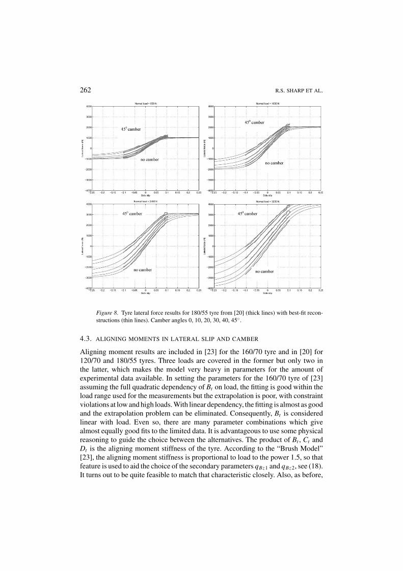
If the cornering motorcycle is excited by regular road undulations, the responseis potentially dangerous if resonance in connection with a lightly damped modeof oscillation occurs [30]. It was found in earlier work that about 15◦ lean islikely to represent a worst case, since, for smaller angles, the road forcing cou-ples only weakly to the lateral oscillatory responses, while for larger angles, themodal damping is likely to increase. Such a 15◦ lean case is illustrated, for aconstant speed of 65 m/s, in Figure 25. The plot shows the steer angle to road dis-placement forcing frequency response gain relative to 1 rad/m, accounting properly


Figure 21. Power contributions as functions of speed in steady turning with 45◦ lean angle.

Figure 22. Motorcycle root locus plot for 15◦ lean angle through speed range 3.3 (squares) to75 (diamonds) m/s. Nominal case – points; frame stiffness halved – circles.

for the time delay between the forcing acting on the front wheel and on the rearwheel, the so-called wheelbase filtering effect. Resonance of the cornering weaveis evident at 26 rad/s forcing frequency, while the wobble is most responsive at50 rad/s.




9. Conclusions

Substantial improvements to an advanced motorcycle dynamics model have beenmade, relating to (a) tyre/road contact geometry; (b) the tyre shear force and mo-ment system; (c) tyre relaxation properties and (d) the monoshock rear suspension


Figure 25. Steer angle response to road undulation forcing of nominal motorcycle at 15◦ leanangle and 65 m/s speed.

mechanism. In particular, parameters for the powerful Magic Formula method,representing the shear forces developed by modern, high performance motorcycletyres have been derived. This provides a readily usable generic description of thesteady-state force and moment system of such tyres, with a very wide range ofvalidity. Also, the geometric treatment of the monoshock suspension system is newand it contributes to computational efficiency. Steady-turning equilibrium force,moment and power checks have been refined and results of high precision showntestify to the model’s accuracy of construction.

Significant progress towards a complete parametric description of a contempo-rary, high performance motorcycle has been made, although a little further workis needed to finish the measurement campaign. The rider upper body structure hasbeen represented as relatively compliant, in sympathy with the rig measurements ofNishimi et al [16]. Results obtained on this basis suggest that the rider upper bodydamping is significantly stabilising to the wobble mode, accounting potentially forthe observation that light riders are more at risk from oscillations than heavier ones.

Steady turning equilibrium states, tyre forces and steer torque requirements havebeen illustrated and the power dissipation through the speed range for steady turningat 45◦ lean angle has been shown for the first time.

Straight running root locus plots, from a linearised version of the model, havesuggested that, despite the relatively high torsional stiffness of many modern frames,it is still important to the stability and control and it needs including in analysis anddesign discussions. Use of the model for the calculation of stability in cornering hasbeen illustrated. Stability margins in cornering typically increase as compared withstraight running, although complex patterns of behaviour are possible. Current work


concerns the nonlinear phenomena, sub-harmonic and super-harmonic oscillations,special operating conditions yielding commensurate relationships between naturalfrequencies and the consequent possibility of internal and combination resonances,and advantageous alternatives to the conventional steering damper for restrainingthe steering system.

Appendix: Motorcycle Parameter Values (SI Units)

Table A.I. Masses.

Mff str Mff sus Mmain Mrw Mfw Mubr Mswg arm9.99 7.25 165.13 14.7 11.9 33.68 8

Table A.II. Inertias.

Iff strx Iff stry Iff strz Iff strxz Imnx Imny Imnz Imnxz Iubrx Iubry

1.341 1.584 0.4125 0 11.085 22.013 14.982 −3.691 1.428 1.347

Iubrz Iubrxz Ifwx Ifwy Irwx Irwy Is ax Is ay Is az

0.916 0.443 0.270 0.484 0.383 0.638 0.02 0.259 0.259

Table A.III. Dimensions (Figures 1, 3, 4 and 16).

x2 z2 x3 z3 x4 z4 x5 z5 x6

1.173 −0.749 1.164 −0.77 1.342 −0.426 1.365 −0.324 1.410

z6 z7 x8 z8 x9 z9 x10 z10 x11

−0.282 −0.297 0.6779 −0.4724 0.364 −0.8438 0.415 −1.14 0.549

z11 x13 z13 x14 z14 x19 z19 x20 z20

−0.3608 0.487 −0.4888 0.196 −0.3113 0.539 −0.1878 0.4946 −0.1522

x21 z21 x22 z22 ε r R0 f R0 l free

0.4443 −0.1782 0.3722 −0.2748 0.4189 0.095 0.06 0.3435

Table A.IV. Limit stop geometry.

r lmax r lmin f dmax f dmin str lim

0.3385 0.2735 0.03 0.07 0.5061

Table A.V. Stiffnesses.

r k f k r kt f kt r krbd f krbd

58570 25000 141000 130000 1e15 1e15

r kcom f kcom kp ubr kp twst kp str k strstop

1e11 1e11 380 100000 0 3e9


Table A.VI. Damping coefficients.

r c f c Cp ubr Cp twst Cp str

11650 2134 34.0 100 6.944

Table A.VII. Aerodynamic parameters.

CD CL CP f Area ρ, density

0.48 0.078 0.189 0.65 1.225

Table A.VIII. Speed and steering control gain coefficients.

drvp drvi spg0 spg1 sig0 sig1 sdg0 sdg1

−500 −1000 −60 −0.6875 −250 1.875 −50 0.6

References

1. Sharp, R.S., ‘Stability, control and steering responses of motorcycles’, Vehicle System Dynamics35(4–5), 2001, 291–318.

2. Koenen, C., ‘The dynamic behaviour of a motorcycle when running straight ahead and whencornering’, Doctoral Dissertation, Delft University, 1983.

3. Wisselman, D., Iffelsberger, D. and Brandlhuber, B., ‘Einsatz eines Fahrdynamik-Simulationsmodells in der Motorradentwicklung bei BMW’, ATZ 95(2), 1993.

4. Breuer, T. and Pruckner, A., ‘Advanced dynamic motorbike analysis and driver simulation’, 13thEuropean ADAMS Users’ Conference, Paris, 1998.

5. Sharp, R.S. and Limebeer, D.J.N., ‘A motorcycle model for stability and control analysis’,Multibody System Dynamics 6(2), 2001, 123–142.

6. Berritta, R., Biral, F. and Garbin, S., ‘Evaluation of motorcycle handling by multibodymodeling and simulation’, Proc. 6th Int. Conf. on High Tech. Engines and Cars, Modena,2000.

7. Cossalter, V. and Lot, R., ‘A motorcycle multi-body model for real time simulations based onthe natural coordinates approach’, Vehicle System Dynamics 37(6), 423–447, 2002.

8. Bio-Astronautus Data Book, NASA SP 3006, 1964.9. Housner, G.W. and Hudson, D.E., Applied Mechanics–Dynamics, 2nd edn., D. Van Nostrand

Company Inc., Princeton, NJ, 1959.10. Pick, A. and Cole, D.J., ‘Neuromuscular dynamics and the vehicle steering task’, in Proc. IAVSD

Symposium on Dynamics of Vehicles on Roads and on Tracks, Kanagawa, Japan, August 2003,in press.

11. Sharp, R.S. and Limebeer, D.J.N., ‘On steering wobble oscillations of motorcycles’, Proc. I.Mech. E., Part C, Journal of Mechanical Engineering Science, in press.

12. Abdelkebir, A., ‘Measurements of inertia, stiffness and damping components of a Suzuki GSX-R1000’, Project work report, Imperial College London, Mechanical Engineering Department,2002.

13. Sharp, R.S. and Alstead, C.J., ‘The influence of structural flexibilities on the straight runningstability of motorcycles’, Vehicle System Dynamics 9(6), 1980, 327–357.

14. Spierings, P.T.J., ‘The effects of lateral front fork flexibility on the vibrational modes of straight-running single track vehicles’, Vehicle System Dynamics 10(1), 1981, 37–38.


15. Giles, C.G. and Sharp, R.S., ‘Static and dynamic stiffness and deflection mode measurements on amotorcycle, with particular reference to steering behaviour’, Proc. I. Mech. E./MIRA Conferenceon Road Vehicle Handling, London, Mechanical Engineering Publications, 1983, 185–192.

16. Nishimi, T., Aoki, A. and Katayama, T., ‘Analysis of straight running stability of motorcycles’,10th International Technical Conf. on Experimental Safety Vehicles, July 1985, 33 pp.

17. Cossalter, V., Doria, A. and Lot, R., ‘Steady turning of two-wheeled vehicles’, Vehicle SystemDynamics 31(3), 1999, 157–181.

18. Cossalter, V., Lot, R. and Fabiano, M., ‘The influence of tire properties on the stability of amotorcycle in straight running and curves’, SAE 2002-01-1572, 2002.

19. Cossalter, V., Motorcycle Dynamics, Race Dynamics, Greendale, WI, 2002.20. de Vries, E.J.H. and Pacejka, H.B., ‘Motorcycle tyre measurements and models’, in Palkovics,

L. (ed.), Proceedings of the 15th IAVSD Symposium on the Dynamics of Vehicles on Roads andon Tracks, 1997 (Suppl. Vehicle System Dynamics) 28, 1998.

21. de Vries, E.J.H. and Pacejka, H.B., ‘The effect of tyre modeling on the stability analysis of amotorcycle’, Proceedings of AVEC’98, Nagoya, SAE of Japan, 1998, 355–360.

22. Tezuka, Y., Ishii, H. and Kiyota, S., ‘Application of the magic formula tire model to motorcyclemaneuverability analysis’, JSAE Review 22, 2001, 305–310.

23. Pacejka, H.B., Tyre and Vehicle Dynamics, Butterworth Heinemann, Oxford, 2002.24. Sakai, H., Kanaya, O. and Iijima, H., ‘Effect of main factors on dynamic properties of motorcycle

tires’, SAE 790259, 1979.25. Cossalter, V., Doria, A., Lot, R., Ruffo, N. and Salvador, M., ‘Dynamic properties of motorcycle

and scooter tires: Measurement and comparison’, Vehicle System Dynamics 39(5), 2003, 329–352.

26. van Oosten, J.J.M., Kuiper, E., Leister, G., Bode, D., Schindler, H., Tischleder, J. and Kohne,S., ‘A new tyre model for TIME measurement data’, in press.

27. Fujioka, T. and Goda, K., ‘Discrete brush tire model for calculating tire forces with large camberangle’, in Segel, L. (ed.), Proceedings of the 14th IAVSD Symposium on the Dynamics of Vehicleson Roads and on Tracks, 1995 (Suppl. Vehicle System Dynamics) 25, 1996.

28. Ishii, H. and Tezuka, Y., ‘Considerations of turning performance for motorcycles’, in Proceedingsof SETC’97, Yokohama, 1997, 383–389 (JSAE 9734601; SAE 972127).

29. Mousseau, C.W., Sayers, M.W. and Fagan, D.J., ‘Symbolic quasi-static and dynamic analyses ofcomplex automobile models’, The Dynamics of Vehicles on Roads and on Tracks, Sauvage, G.(ed.), in Proceedings of the 12th IAVSD Symposium, Swets and Zeitlinger, Lisse, 1992, 446–459.

30. Limebeer, D.J.N., Sharp, R.S. and Evangelou, S., ‘Motorcycle steering oscillations due to roadprofiling’, Proc. ASME, Journal of Applied Mechanics 69(6), 2002, 724–739.

Documents

Advances in the Modelling of Motorcycle Dynamics · ADVANCES IN THE MODELLING OF MOTORCYCLE DYNAMICS 253 Figure 1. Scaled diagrammatic motorcycle in side view. 2.2. INERTIAS AND …