Advances in Water Resources - TU Braunschweig Now at the Laboratory of Soil and Environmental Physics, EPF Lausanne. ... Advances in Water Resources xxx (2008) xxx–xxx Contents lists

Advances in Water Resources xxx (2008) xxx–xxx

ARTICLE IN PRESS

Contents lists available at ScienceDirect

Advances in Water Resources

journal homepage: www.elsevier .com/ locate/advwatres

Prediction of capillary hysteresis in a porous material using lattice-Boltzmannmethods and comparison to experimental data and a morphological porenetwork model

B. Ahrenholz a, J. Tölke a,*, P. Lehmann b,1, A. Peters c, A. Kaestner b,2, M. Krafczyk a, W. Durner c

a Institute for Computational Modeling in Civil Engineering, TU Braunschweig, Pockelsstrasse 3, Germanyb Institute of Terrestrial EcoSystems, ETH Zürich, Universitätstrasse 16, Switzerlandc GeoEcology and Soil Science, TU Braunschweig, Langer Kamp 19c, Germany

a r t i c l e i n f o

Article history:Received 23 March 2007Received in revised form 18 March 2008Accepted 23 March 2008Available online xxxx

Keywords:Capillary hysteresisPore scale modelingLattice-BoltzmannMorphological pore network model

0309-1708/$ - see front matter � 2008 Elsevier Ltd. Adoi:10.1016/j.advwatres.2008.03.009

* Corresponding author.E-mail address: [email protected] (J. Tölke).

1 Now at the Laboratory of Soil and Environmental P2 Now at Varian Medical Systems, Imaging Laborato

Please cite this article in press as: Ahrenho(2008), doi:10.1016/j.advwatres.2008.03.0

a b s t r a c t

In this work we use two numerical methods which rely only on the geometry and material parameters topredict capillary hysteresis in a porous material. The first numerical method is a morphological pore net-work (MPN) model, where structural elements are inserted into the imaged pore space to quantify thelocal capillary forces. Then, based on an invasion–percolation mechanism, the fluid distribution is com-puted. The second numerical method is a lattice-Boltzmann (LB) approach which solves the coupledNavier–Stokes equations for both fluid phases and describes the dynamics of the fluid/fluid interface.We have developed an optimized version of the model proposed in [Tölke J, Freudiger S, Krafczyk M.An adaptive scheme for LBE multiphase flow simulations on hierarchical grids, Comput. Fluids2006;35:820–30] for the type of flow problems encountered in this work. A detailed description of themodel and an extensive validation of different multiphase test cases have been carried out. We investi-gated pendular rings in a sphere packing, static and dynamic capillary bundle models and the residualsaturation in a sphere packing.

A sample of 15 mm in diameter filled with sand particles ranging from 100 to 500 lm was scannedusing X-rays from a synchrotron source with a spatial resolution of 11 lm. Based on this geometry wecomputed the primary drainage, the first imbibition and the secondary drainage branch of the hysteresisloop using both approaches. For the LB approach, we investigated the dependence of the hysteresis loopon the speed of the drainage and the imbibition process. Furthermore we carried out a sensitivity analysisby simulating the hysteretic effect in several subcubes of the whole geometry with extremal character-istic properties. The predicted hysteretic water retention curves were compared to the results of labora-tory experiments using inverse modeling based on the Richards equation.

A good agreement for the hysteresis loop between the LB and MPN model has been obtained. The pri-mary and secondary drainage of the hysteresis loop of the LB and MPN model compare very well, and alsothe experimental results fit well with a slight offset of 10% in the amplitude. Differences for the first imbi-bition have been observed, but also large differences between two different experimental runs have beenobserved.

� 2008 Elsevier Ltd. All rights reserved.

1. Introduction

In multiphase flow systems of two immiscible phases like airand water in a porous medium like a soil the flow and transportproperties depend on the amount and the spatial distribution ofthe phases within the pore space. On the pore scale the phase dis-tribution is controlled by the capillary forces depending on pore

ll rights reserved.

hysics, EPF Lausanne.ry GmbH, Baden-Dättwil.

lz B et al., Prediction of capill09

size, surface tension, and wettability. For that reason, the relation-ship between capillary pressure and liquid saturation (Pc–Sw rela-tionship) is of high importance for the prediction of water flowand solute transport. Unfortunately, this relationship is ambiguousand depends on the preceding wetting and drainage processes.This phenomenon is denoted as hysteresis and was first docu-mented by Haines in [2]. It is caused by different pore structuresrelevant for drainage and wetting processes. While the drainageof a large pore body may be prevented by surrounding small porethroats, the wetting of fine pores above a large pore is hampered bythe weak capillary forces in the wide body. Additional hysteresiseffects are caused by a difference in advancing and receding

ary hysteresis in a porous material using lattice-Boltzmann ..., Adv

mailto:[email protected]

http://www.sciencedirect.com/science/journal/03091708

http://www.elsevier.com/locate/advwatres

2 B. Ahrenholz et al. / Advances in Water Resources xxx (2008) xxx–xxx

ARTICLE IN PRESS

contact angle [3] and the inclusion of air in a first wetting process.Due to the inclusion of air in a wetting process, the water satura-tion after the primary drainage of a completely saturated porousmedium remains smaller than the porosity for any following wet-ting processes. After a few drainage and wetting cycles, twobounding curves, denoted as main wetting and main drainagebranch, can be determined. All processes within these boundingcurves are denoted as scanning curves. To model water flow andsolute transport correctly, the hysteretic relationship between cap-illary pressure and fluid saturation must be taken into account[4,5]. To quantify the hysteresis and the scanning curves, differentapproaches can be distinguished. On the macroscopic scale, theshape of the scanning curves can be deduced from the main wet-ting and drainage curves. With such a similarity or scaling ap-proach, the shape of any scanning curve can be described [6–8].While most approaches are based on the main drainage and wet-ting curve, it is possible to compute the whole hysteresis loopbased on a single main curve [9]. In addition to these scaling ap-proaches, two new descriptions on the macroscale based on thehysteron (the simplest hysteretic system described by an operator[10]) and the quantification of the continuous and non-continuousfluid phases [11] were recently introduced.

Secondly, the range of liquid saturation as a function of capillarypressure for wetting and drainage processes can be determinedusing pore network models. With a pore model consisting of apore-body and a pore-throat distribution, the hysteresis of thehydraulic functions can be reproduced. The first pore network ap-proaches were limited to cylindrical pore throats on a rectangularlattice [12]. To enhance the flexibility and to develop more realisticpore network models, different throat shapes [13] and other latticetypes [14] were introduced. The drawback of these approaches isthe uncertainty of the pore-throat and pore-body distributionfunction which are obtained from fitting, based on measuredretention functions.

Alternatively, the pore size distribution can be deduced fromimages of the pore space. In Øren et al. [15] the reconstructed porespace is transformed into a pore network that is used as input to atwo-phase network model. Based on this work Valvatne et al. [16]constructed a network with the same topology as a scanned sand-stone sample and modified the size distribution to obtain the samepermeability. To apply this network to other media, the maindrainage branch must be fitted to describe the wetting branch.

Finally, to predict the hysteresis loops without any fitting basedon the measured pore space geometry, a direct numerical simula-tion of the two-phase Stokes problem can be performed. A suitablemethod for this task is the lattice-Boltzmann method. Pan et al.[17] applied successfully a lattice-Boltzmann approach based onthe Shan–Chen [18] multiphase extension for a packing of glassbeads and compared the results to experiments. Nevertheless thisapproach needs numerical experiments to determine the materialparameters. In a later study [19] the focus moved to the determi-nation of relative permeabilities. By using a multiple-relaxation-time (MRT) lattice-Boltzmann approach, more realistic capillarynumbers could be reproduced. In [20] the primary drainage curve(without hysteretic effects) for a porous medium was simulated bya lattice-Boltzmann approach. The medium consisted of sinteredglass and the geometry was obtained by tomography. The LB re-sults were compared to the results of a full-morphological and apore network model and a good agreement for the three modelswas observed. However, these results have not been compared toexperimental data.

In this study we use a MPN model and an LB approach to predicthysteresis in the capillary pressure–saturation relationship for themeasured pore structure of a sand sample. The LB approach isbased on the multiple-relaxation-time (MRT) model with an opti-mized multiphase extension given in [1] and further optimized

Please cite this article in press as: Ahrenholz B et al., Prediction of capill(2008), doi:10.1016/j.advwatres.2008.03.009

for Stokes flow in porous media. This approach permits higher vis-cosity ratios and lower capillary numbers than previous LB multi-phase extensions. To obtain a geometric representation suitable forthe LB solver, the surface of the sand particles was reconstructedfrom the voxel matrix by a marching-cube algorithm and thedescription of the fluid behavior at the solid walls was improvedby the accurate determination of the distance of the fluid nodesto the particle boundaries [21]. Also the numerical resolution ofthe setups was higher as in previous studies. An extensive valida-tion for the model developed has been carried out. Complex testcases like pendular rings, a (dynamic) capillary tube bundle andthe residual water saturation in a periodic array of spheres areset up and analyzed in detail.

We compare our predictions for the capillary hysteresis usingthe MPN and LB model to laboratory measurements, where inversemodeling based on the Richards equation was applied to computethe drainage and imbibition curves. In addition, a few equilibriumstates between water saturation and capillary pressure were ana-lyzed to validate the results of the inverse modeling.

Furthermore we carried out a sensitivity analysis by simulatingthe hysteresis in several subcubes of the whole geometry withextremal characteristic properties.

The paper is organized as follows: In Section 2 the laboratoryexperiments and the methods to determine the hysteresis curvesby an inverse fitting procedure are described. Section 3 introducesthe morphological pore network model and the results for the cap-illary hysteresis. Section 4 discusses the lattice-Boltzmann ap-proach and the results for the saturated permeability and thecapillary hysteresis. In Section 5 the results for the different modelsare compared and conclusions are given. In Appendix A a detaileddescription of the lattice-Boltzmann model is given and in Appen-dix B various test cases for multiphase flows are carried out to val-idate the lattice-Boltzmann method.

2. Material, experimental setup and inverse parameter fit

2.1. Materials and samples

To predict the fluid distribution within the pore structure wescanned a sand sample of 1.5 cm in diameter and 1 cm in heightusing X-rays from a synchrotron source. The tomography was car-ried out at the Hamburger Synchrotron Laboratories (HASYLAB) inGermany. The particle size of the sand material ranged from 0.1 to0.5 mm. Based on the imaged X-ray attenuation the density distri-bution of the solid material can be reconstructed. The recon-structed density map was segmented into a black and whiteimage of pore space and solid phase with a voxel resolution ofrv = 11 lm. A voxel (volumetric pixel) is a volume element, repre-senting a value on a Cartesian grid in three-dimensional spaceand is commonly used as the basic unit of a three-dimensional im-age. The tomography of this sand material is described in more de-tail in [22]. To avoid effects at the boundary between the sand andthe container, a cube from the center of the cylinder with 8003 vox-els was analyzed with respect to geometrical properties and fluiddistribution. In case of the lattice-Boltzmann approach the compu-tation of the hysteresis in the relationship between capillary pres-sure and liquid saturation is very time consuming and wasdetermined for a subcube with 2003 voxels. The results may de-pend on the chosen section within the whole sample with 8003

voxels. To estimate the sensitivity of the results on the chosen sec-tion, we focused on two subcubes with extremal properties. Forthat purpose, we computed characteristic geometrical propertiesfor various subcubes. We shifted the origin of the analyzed sub-cube in intervals of 20 voxels in x-, y- and z-direction from position0,0,0 to 600,600,600 within the large image. Totally, 313 = 29,791


0 2 4 6 8 10 12x 105

5000

4000

3000

2000

1000

0

p LB[P

a]

time [sec]

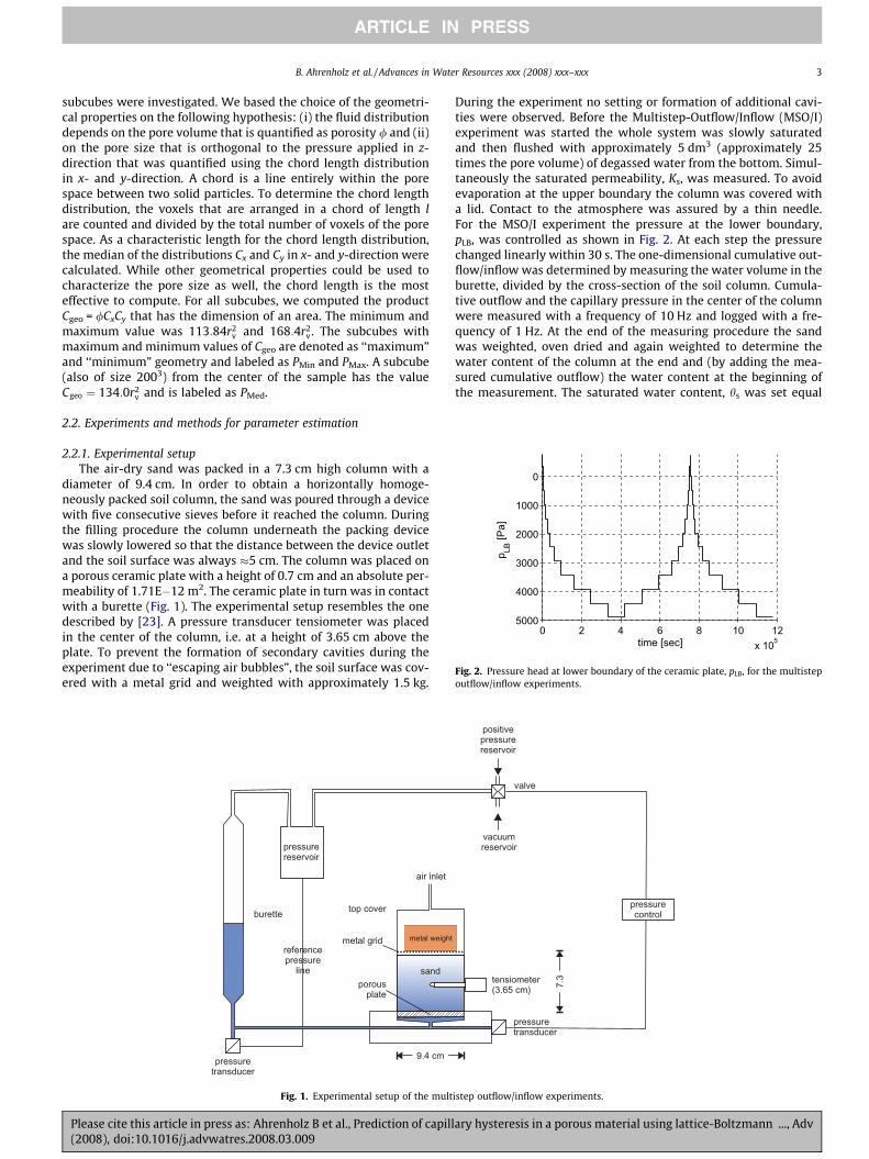
Fig. 2. Pressure head at lower boundary of the ceramic plate, pLB, for the multistepoutflow/inflow experiments.

B. Ahrenholz et al. / Advances in Water Resources xxx (2008) xxx–xxx 3

ARTICLE IN PRESS

subcubes were investigated. We based the choice of the geometri-cal properties on the following hypothesis: (i) the fluid distributiondepends on the pore volume that is quantified as porosity / and (ii)on the pore size that is orthogonal to the pressure applied in z-direction that was quantified using the chord length distributionin x- and y-direction. A chord is a line entirely within the porespace between two solid particles. To determine the chord lengthdistribution, the voxels that are arranged in a chord of length lare counted and divided by the total number of voxels of the porespace. As a characteristic length for the chord length distribution,the median of the distributions Cx and Cy in x- and y-direction werecalculated. While other geometrical properties could be used tocharacterize the pore size as well, the chord length is the mosteffective to compute. For all subcubes, we computed the productCgeo = /CxCy that has the dimension of an area. The minimum andmaximum value was 113:84r2

v and 168:4r2v. The subcubes with

maximum and minimum values of Cgeo are denoted as ‘‘maximum”and ‘‘minimum” geometry and labeled as PMin and PMax. A subcube(also of size 2003) from the center of the sample has the valueCgeo ¼ 134:0r2

v and is labeled as PMed.

2.2. Experiments and methods for parameter estimation

2.2.1. Experimental setupThe air-dry sand was packed in a 7.3 cm high column with a

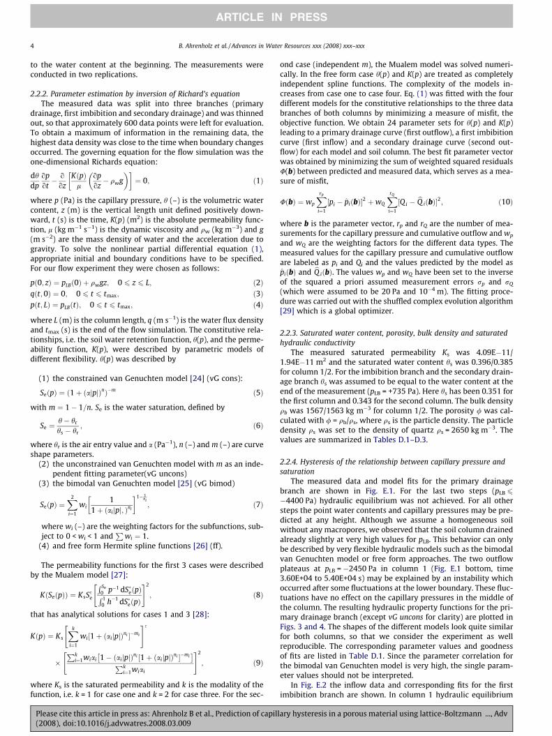
diameter of 9.4 cm. In order to obtain a horizontally homoge-neously packed soil column, the sand was poured through a devicewith five consecutive sieves before it reached the column. Duringthe filling procedure the column underneath the packing devicewas slowly lowered so that the distance between the device outletand the soil surface was always �5 cm. The column was placed ona porous ceramic plate with a height of 0.7 cm and an absolute per-meability of 1.71E�12 m2. The ceramic plate in turn was in contactwith a burette (Fig. 1). The experimental setup resembles the onedescribed by [23]. A pressure transducer tensiometer was placedin the center of the column, i.e. at a height of 3.65 cm above theplate. To prevent the formation of secondary cavities during theexperiment due to ‘‘escaping air bubbles”, the soil surface was cov-ered with a metal grid and weighted with approximately 1.5 kg.

sand

9.4 cm

pressurereservoir

pressuretransducer

burette

porousplate

air inlet

top cover

referencepressure

line

metal weightmetal grid

Fig. 1. Experimental setup of the mult


During the experiment no setting or formation of additional cavi-ties were observed. Before the Multistep-Outflow/Inflow (MSO/I)experiment was started the whole system was slowly saturatedand then flushed with approximately 5 dm3 (approximately 25times the pore volume) of degassed water from the bottom. Simul-taneously the saturated permeability, Ks, was measured. To avoidevaporation at the upper boundary the column was covered witha lid. Contact to the atmosphere was assured by a thin needle.For the MSO/I experiment the pressure at the lower boundary,pLB, was controlled as shown in Fig. 2. At each step the pressurechanged linearly within 30 s. The one-dimensional cumulative out-flow/inflow was determined by measuring the water volume in theburette, divided by the cross-section of the soil column. Cumula-tive outflow and the capillary pressure in the center of the columnwere measured with a frequency of 10 Hz and logged with a fre-quency of 1 Hz. At the end of the measuring procedure the sandwas weighted, oven dried and again weighted to determine thewater content of the column at the end and (by adding the mea-sured cumulative outflow) the water content at the beginning ofthe measurement. The saturated water content, hs was set equal

tensiometer(3.65 cm)

pressurecontrol

valve

vacuumreservoir

7.3

pressuretransducer

positivepressurereservoir

istep outflow/inflow experiments.



ARTICLE IN PRESS

to the water content at the beginning. The measurements wereconducted in two replications.

2.2.2. Parameter estimation by inversion of Richard’s equationThe measured data was split into three branches (primary

drainage, first imbibition and secondary drainage) and was thinnedout, so that approximately 600 data points were left for evaluation.To obtain a maximum of information in the remaining data, thehighest data density was close to the time when boundary changesoccurred. The governing equation for the flow simulation was theone-dimensional Richards equation:

dhdp

opot� o

ozKðpÞ

lopoz� qwg

� �� ¼ 0; ð1Þ

where p (Pa) is the capillary pressure, h (–) is the volumetric watercontent, z (m) is the vertical length unit defined positively down-ward, t (s) is the time, K(p) (m2) is the absolute permeability func-tion, l (kg m�1 s�1) is the dynamic viscosity and qw (kg m�3) and g(m s�2) are the mass density of water and the acceleration due togravity. To solve the nonlinear partial differential equation (1),appropriate initial and boundary conditions have to be specified.For our flow experiment they were chosen as follows:

pð0; zÞ ¼ pLBð0Þ þ qwgz; 0 6 z 6 L; ð2Þqðt;0Þ ¼ 0; 0 6 t 6 tmax; ð3Þpðt; LÞ ¼ pLBðtÞ; 0 6 t 6 tmax; ð4Þ

where L (m) is the column length, q (m s�1) is the water flux densityand tmax (s) is the end of the flow simulation. The constitutive rela-tionships, i.e. the soil water retention function, h(p), and the perme-ability function, K(p), were described by parametric models ofdifferent flexibility. h(p) was described by

(1) the constrained van Genuchten model [24] (vG cons):

SeðpÞ ¼ ð1þ ðajpjÞnÞ�m ð5Þ

with m ¼ 1� 1=n. Se is the water saturation, defined by

Se ¼h� hr

hs � hr; ð6Þ

where hr is the air entry value and a (Pa�1), n (–) and m (–) are curveshape parameters.

(2) the unconstrained van Genuchten model with m as an inde-pendent fitting parameter(vG uncons)

(3) the bimodal van Genuchten model [25] (vG bimod)

SeðpÞ ¼X2

i¼1

wi1

1þ ðaijpj; Þni

� �1� 1ni

; ð7Þ

where wi (–) are the weighting factors for the subfunctions, sub-ject to 0 < wi < 1 and

Pwi ¼ 1.

(4) and free form Hermite spline functions [26] (ff).

The permeability functions for the first 3 cases were describedby the Mualem model [27]:

KðSeðpÞÞ ¼ KsSse

R Se

0 p�1 dS�eðpÞR 10 h�1 dS�eðpÞ

" #2

; ð8Þ

that has analytical solutions for cases 1 and 3 [28]:

KðpÞ ¼ Ks

Xk

i¼1

wi½1þ ðaijpjÞni ��mi

" #s

�Pk

i¼1wiai 1� ðaijpjÞni ½1þ ðaijpjÞni ��mi� �Pk

i¼1wiai

" #2

; ð9Þ

where Ks is the saturated permeability and k is the modality of thefunction, i.e. k = 1 for case one and k = 2 for case three. For the sec-


ond case (independent m), the Mualem model was solved numeri-cally. In the free form case h(p) and K(p) are treated as completelyindependent spline functions. The complexity of the models in-creases from case one to case four. Eq. (1) was fitted with the fourdifferent models for the constitutive relationships to the three databranches of both columns by minimizing a measure of misfit, theobjective function. We obtain 24 parameter sets for h(p) and K(p)leading to a primary drainage curve (first outflow), a first imbibitioncurve (first inflow) and a secondary drainage curve (second out-flow) for each model and soil column. The best fit parameter vectorwas obtained by minimizing the sum of weighted squared residualsU(b) between predicted and measured data, which serves as a mea-sure of misfit,

UðbÞ ¼ wp

Xrp

i¼1

½pi � p̂iðbÞ�2 þwQ

XrQ

i¼1

½Q i � bQ iðbÞ�2; ð10Þ

where b is the parameter vector, rp and rQ are the number of mea-surements for the capillary pressure and cumulative outflow and wp

and wQ are the weighting factors for the different data types. Themeasured values for the capillary pressure and cumulative outfloware labeled as pi and Qi and the values predicted by the model asp̂iðbÞ and bQ iðbÞ. The values wp and wQ have been set to the inverseof the squared a priori assumed measurement errors rp and rQ

(which were assumed to be 20 Pa and 10�4 m). The fitting proce-dure was carried out with the shuffled complex evolution algorithm[29] which is a global optimizer.

2.2.3. Saturated water content, porosity, bulk density and saturatedhydraulic conductivity

The measured saturated permeability Ks was 4.09E�11/1.94E�11 m2 and the saturated water content hs was 0.396/0.385for column 1/2. For the imbibition branch and the secondary drain-age branch hs was assumed to be equal to the water content at theend of the measurement (pLB = +735 Pa). Here hs has been 0.351 forthe first column and 0.343 for the second column. The bulk densityqb was 1567/1563 kg m�3 for column 1/2. The porosity / was cal-culated with / = qb/qs, where qs is the particle density. The particledensity qs was set to the density of quartz qs = 2650 kg m�3. Thevalues are summarized in Tables D.1–D.3.

2.2.4. Hysteresis of the relationship between capillary pressure andsaturation

The measured data and model fits for the primary drainagebranch are shown in Fig. E.1. For the last two steps (pLB 6

�4400 Pa) hydraulic equilibrium was not achieved. For all othersteps the point water contents and capillary pressures may be pre-dicted at any height. Although we assume a homogeneous soilwithout any macropores, we observed that the soil column drainedalready slightly at very high values for pLB. This behavior can onlybe described by very flexible hydraulic models such as the bimodalvan Genuchten model or free form approaches. The two outflowplateaus at pLB = �2450 Pa in column 1 (Fig. E.1 bottom, time3.60E+04 to 5.40E+04 s) may be explained by an instability whichoccurred after some fluctuations at the lower boundary. These fluc-tuations have no effect on the capillary pressures in the middle ofthe column. The resulting hydraulic property functions for the pri-mary drainage branch (except vG uncons for clarity) are plotted inFigs. 3 and 4. The shapes of the different models look quite similarfor both columns, so that we consider the experiment as wellreproducible. The corresponding parameter values and goodnessof fits are listed in Table D.1. Since the parameter correlation forthe bimodal van Genuchten model is very high, the single param-eter values should not be interpreted.

In Fig. E.2 the inflow data and corresponding fits for the firstimbibition branch are shown. In column 1 hydraulic equilibrium


Fig. 4. Capillary hysteresis, Column 2. Solid lines: primary drainage; dots: first imbibition; dashed lines: secondary drainage.

Fig. 3. Capillary hysteresis, Column 1. Solid lines: primary drainage; dots: first imbibition; dashed lines: secondary drainage.


ARTICLE IN PRESS

is only reached after pLB P �980 Pa. This late response to thechange of the pressure at the lower boundary could possibly beexplained by the existence of some small air bubbles underneaththe ceramic plate which cause contact problems of the waterphase. These air bubbles were not visible. Due to this late re-sponse almost the complete inflow happened in the last pressuresteps. This can only be described by a very steep retention func-tion close to saturation. The fit with both unimodal models failedcompletely. The data for column 2 looks more reasonable. Butalso here the system behavior can only be described adequatelyby the more flexible models, i.e. the bimodal or the free form ap-proaches. The hydraulic properties functions for the first imbibi-tion branch are shown in Figs. 3 and 4 and the correspondingparameter values are given in Table D.2. Due to the assumptionthat the imbibition measurement for column 1 was influencedby some measurement artifacts we suggest that the hydraulicproperties functions for the imbibition branch are interpretedonly from column 2.


The measured data and resulting fits for the secondary drainagebranch are shown in Fig. E.3. Again, the behavior close to saturationcan only adequately be described by the more flexible functions.The resulting hydraulic properties functions are plotted in Figs. 3and 4. Again, the shapes of the different models look quite similarfor both columns, so that we consider the experiment as wellreproducible. The corresponding parameter values and goodnessof fits are listed in Table D.3.

2.2.5. Equilibrium fitIn addition, a few equilibrium states between water saturation

and capillary pressure were analyzed to validate the results of theinverse modeling. The hydraulic equilibrium data (values at theend of each pressure step until pLB = �3900 Pa leading to 10 datapoints) for the four outflow branches has been fitted with the threeparametric models as described in [30] with the software toolSHYPFIT2.0 (Soil Hydraulic Properties Fitting). The results are veryclose to the previous results and are not given here.



ARTICLE IN PRESS

3. Morphological pore network model

We give a short description of the basics of the morphologicalpore network model. For a more detailed description we refer to[31,32]. The computation of the water retention curve with a mor-phological pore network model is based on a two-step procedure.Firstly, a size is assigned to each voxel of the pore space. In a sec-ond step, the replacement of a fluid phase by an invading fluid isdescribed as an invasion percolation process. To determine thepore size, structural elements are inserted into the pore space. Incase of the drainage step that is controlled by the narrowest struc-tures, spheres with an increasing diameter are centered at eachvoxel of the pore space until the sphere is touching the solid phase.The radius of the sphere corresponds to the distance to the solid

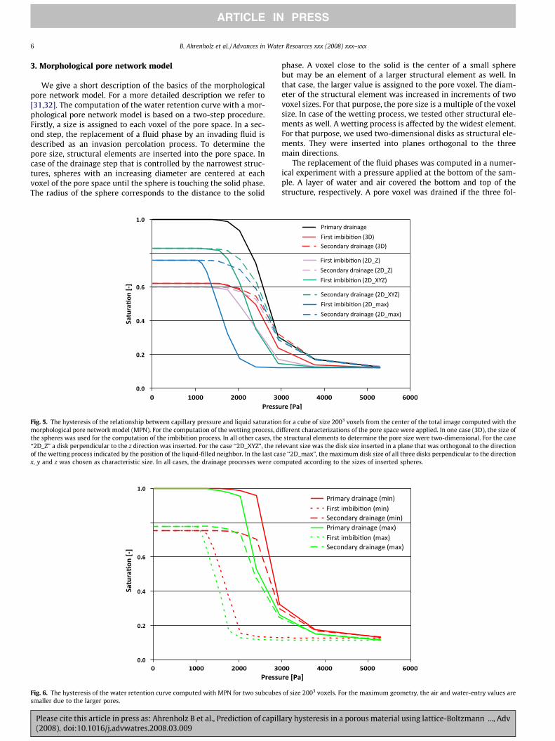
Fig. 5. The hysteresis of the relationship between capillary pressure and liquid saturationmorphological pore network model (MPN). For the computation of the wetting process, dthe spheres was used for the computation of the imbibition process. In all other cases, the‘‘2D_Z” a disk perpendicular to the z direction was inserted. For the case ‘‘2D_XYZ”, the reof the wetting process indicated by the position of the liquid-filled neighbor. In the last cax, y and z was chosen as characteristic size. In all cases, the drainage processes were co

Fig. 6. The hysteresis of the water retention curve computed with MPN for two subcubessmaller due to the larger pores.


phase. A voxel close to the solid is the center of a small spherebut may be an element of a larger structural element as well. Inthat case, the larger value is assigned to the pore voxel. The diam-eter of the structural element was increased in increments of twovoxel sizes. For that purpose, the pore size is a multiple of the voxelsize. In case of the wetting process, we tested other structural ele-ments as well. A wetting process is affected by the widest element.For that purpose, we used two-dimensional disks as structural ele-ments. They were inserted into planes orthogonal to the threemain directions.

The replacement of the fluid phases was computed in a numer-ical experiment with a pressure applied at the bottom of the sam-ple. A layer of water and air covered the bottom and top of thestructure, respectively. A pore voxel was drained if the three fol-

for a cube of size 2003 voxels from the center of the total image computed with theifferent characterizations of the pore space were applied. In one case (3D), the size of

structural elements to determine the pore size were two-dimensional. For the caselevant size was the disk size inserted in a plane that was orthogonal to the directionse ‘‘2D_max”, the maximum disk size of all three disks perpendicular to the directionmputed according to the sizes of inserted spheres.

of size 2003 voxels. For the maximum geometry, the air and water-entry values are



ARTICLE IN PRESS

lowing conditions are fulfilled (for the reverse wetting process, theconditions are given in parentheses):

(i) the size dependent capillary forces are smaller (larger) thanthe applied pressure,

(ii) the water (air) in the pore is connected to the water at thebottom (air at the top) and

(iii) air (or water) connected to the air at the top (water at thebottom) is in a neighbored pore voxel.

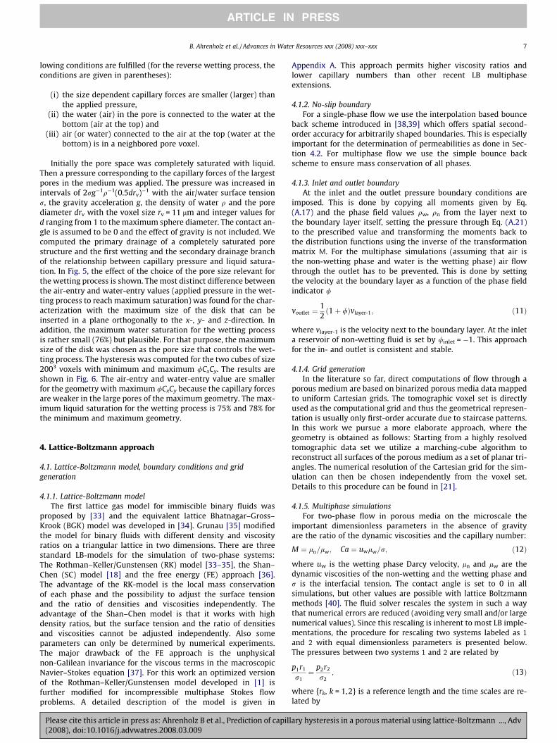
Initially the pore space was completely saturated with liquid.Then a pressure corresponding to the capillary forces of the largestpores in the medium was applied. The pressure was increased inintervals of 2rg�1q�1(0.5drv)�1 with the air/water surface tensionr, the gravity acceleration g, the density of water q and the porediameter drv with the voxel size rv = 11 lm and integer values ford ranging from 1 to the maximum sphere diameter. The contact an-gle is assumed to be 0 and the effect of gravity is not included. Wecomputed the primary drainage of a completely saturated porestructure and the first wetting and the secondary drainage branchof the relationship between capillary pressure and liquid satura-tion. In Fig. 5, the effect of the choice of the pore size relevant forthe wetting process is shown. The most distinct difference betweenthe air-entry and water-entry values (applied pressure in the wet-ting process to reach maximum saturation) was found for the char-acterization with the maximum size of the disk that can beinserted in a plane orthogonally to the x-, y- and z-direction. Inaddition, the maximum water saturation for the wetting processis rather small (76%) but plausible. For that purpose, the maximumsize of the disk was chosen as the pore size that controls the wet-ting process. The hysteresis was computed for the two cubes of size2003 voxels with minimum and maximum /CxCy. The results areshown in Fig. 6. The air-entry and water-entry value are smallerfor the geometry with maximum /CxCy because the capillary forcesare weaker in the large pores of the maximum geometry. The max-imum liquid saturation for the wetting process is 75% and 78% forthe minimum and maximum geometry.

4. Lattice-Boltzmann approach

4.1. Lattice-Boltzmann model, boundary conditions and gridgeneration

4.1.1. Lattice-Boltzmann modelThe first lattice gas model for immiscible binary fluids was

proposed by [33] and the equivalent lattice Bhatnagar–Gross–Krook (BGK) model was developed in [34]. Grunau [35] modifiedthe model for binary fluids with different density and viscosityratios on a triangular lattice in two dimensions. There are threestandard LB-models for the simulation of two-phase systems:The Rothman–Keller/Gunstensen (RK) model [33–35], the Shan–Chen (SC) model [18] and the free energy (FE) approach [36].The advantage of the RK-model is the local mass conservationof each phase and the possibility to adjust the surface tensionand the ratio of densities and viscosities independently. Theadvantage of the Shan–Chen model is that it works with highdensity ratios, but the surface tension and the ratio of densitiesand viscosities cannot be adjusted independently. Also someparameters can only be determined by numerical experiments.The major drawback of the FE approach is the unphysicalnon-Galilean invariance for the viscous terms in the macroscopicNavier–Stokes equation [37]. For this work an optimized versionof the Rothman–Keller/Gunstensen model developed in [1] isfurther modified for incompressible multiphase Stokes flowproblems. A detailed description of the model is given in


Appendix A. This approach permits higher viscosity ratios andlower capillary numbers than other recent LB multiphaseextensions.

4.1.2. No-slip boundaryFor a single-phase flow we use the interpolation based bounce

back scheme introduced in [38,39] which offers spatial second-order accuracy for arbitrarily shaped boundaries. This is especiallyimportant for the determination of permeabilities as done in Sec-tion 4.2. For multiphase flow we use the simple bounce backscheme to ensure mass conservation of all phases.

4.1.3. Inlet and outlet boundaryAt the inlet and the outlet pressure boundary conditions are

imposed. This is done by copying all moments given by Eq.(A.17) and the phase field values qw, qn from the layer next tothe boundary layer itself, setting the pressure through Eq. (A.21)to the prescribed value and transforming the moments back tothe distribution functions using the inverse of the transformationmatrix M. For the multiphase simulations (assuming that air isthe non-wetting phase and water is the wetting phase) air flowthrough the outlet has to be prevented. This is done by settingthe velocity at the boundary layer as a function of the phase fieldindicator /

voutlet ¼12ð1þ /Þvlayer-1; ð11Þ

where vlayer-1 is the velocity next to the boundary layer. At the inleta reservoir of non-wetting fluid is set by /inlet = �1. This approachfor the in- and outlet is consistent and stable.

4.1.4. Grid generationIn the literature so far, direct computations of flow through a

porous medium are based on binarized porous media data mappedto uniform Cartesian grids. The tomographic voxel set is directlyused as the computational grid and thus the geometrical represen-tation is usually only first-order accurate due to staircase patterns.In this work we pursue a more elaborate approach, where thegeometry is obtained as follows: Starting from a highly resolvedtomographic data set we utilize a marching-cube algorithm toreconstruct all surfaces of the porous medium as a set of planar tri-angles. The numerical resolution of the Cartesian grid for the sim-ulation can then be chosen independently from the voxel set.Details to this procedure can be found in [21].

4.1.5. Multiphase simulationsFor two-phase flow in porous media on the microscale the

important dimensionless parameters in the absence of gravityare the ratio of the dynamic viscosities and the capillary number:

M ¼ ln=lw; Ca ¼ uwlw=r; ð12Þ

where uw is the wetting phase Darcy velocity, ln and lw are thedynamic viscosities of the non-wetting and the wetting phase andr is the interfacial tension. The contact angle is set to 0 in allsimulations, but other values are possible with lattice Boltzmannmethods [40]. The fluid solver rescales the system in such a waythat numerical errors are reduced (avoiding very small and/or largenumerical values). Since this rescaling is inherent to most LB imple-mentations, the procedure for rescaling two systems labeled as 1

and 2 with equal dimensionless parameters is presented below.The pressures between two systems 1 and 2 are related by

p1r1

r1¼ p2r2

r2; ð13Þ

where {rk, k = 1,2} is a reference length and the time scales are re-lated by


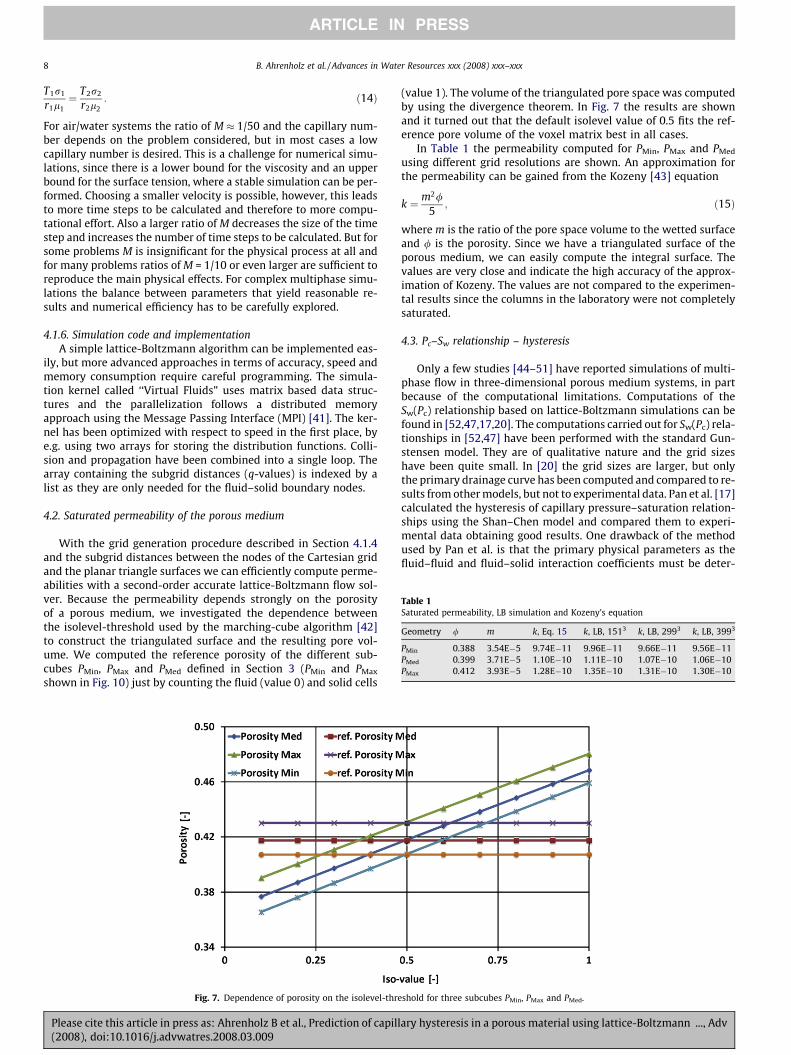
Table 1Saturated permeability, LB simulation and Kozeny’s equation

Geometry / m k, Eq. 15 k, LB, 1513 k, LB, 2993 k, LB, 3993

PMin 0.388 3.54E�5 9.74E�11 9.96E�11 9.66E�11 9.56E�11PMed 0.399 3.71E�5 1.10E�10 1.11E�10 1.07E�10 1.06E�10PMax 0.412 3.93E�5 1.28E�10 1.35E�10 1.31E�10 1.30E�10


ARTICLE IN PRESS

T1r1

r1l1¼ T2r2

r2l2: ð14Þ

For air/water systems the ratio of M � 1/50 and the capillary num-ber depends on the problem considered, but in most cases a lowcapillary number is desired. This is a challenge for numerical simu-lations, since there is a lower bound for the viscosity and an upperbound for the surface tension, where a stable simulation can be per-formed. Choosing a smaller velocity is possible, however, this leadsto more time steps to be calculated and therefore to more compu-tational effort. Also a larger ratio of M decreases the size of the timestep and increases the number of time steps to be calculated. But forsome problems M is insignificant for the physical process at all andfor many problems ratios of M = 1/10 or even larger are sufficient toreproduce the main physical effects. For complex multiphase simu-lations the balance between parameters that yield reasonable re-sults and numerical efficiency has to be carefully explored.

4.1.6. Simulation code and implementationA simple lattice-Boltzmann algorithm can be implemented eas-

ily, but more advanced approaches in terms of accuracy, speed andmemory consumption require careful programming. The simula-tion kernel called ‘‘Virtual Fluids” uses matrix based data struc-tures and the parallelization follows a distributed memoryapproach using the Message Passing Interface (MPI) [41]. The ker-nel has been optimized with respect to speed in the first place, bye.g. using two arrays for storing the distribution functions. Colli-sion and propagation have been combined into a single loop. Thearray containing the subgrid distances (q-values) is indexed by alist as they are only needed for the fluid–solid boundary nodes.

4.2. Saturated permeability of the porous medium

With the grid generation procedure described in Section 4.1.4and the subgrid distances between the nodes of the Cartesian gridand the planar triangle surfaces we can efficiently compute perme-abilities with a second-order accurate lattice-Boltzmann flow sol-ver. Because the permeability depends strongly on the porosityof a porous medium, we investigated the dependence betweenthe isolevel-threshold used by the marching-cube algorithm [42]to construct the triangulated surface and the resulting pore vol-ume. We computed the reference porosity of the different sub-cubes PMin, PMax and PMed defined in Section 3 (PMin and PMax

shown in Fig. 10) just by counting the fluid (value 0) and solid cells

Fig. 7. Dependence of porosity on the isolevel-thre


(value 1). The volume of the triangulated pore space was computedby using the divergence theorem. In Fig. 7 the results are shownand it turned out that the default isolevel value of 0.5 fits the ref-erence pore volume of the voxel matrix best in all cases.

In Table 1 the permeability computed for PMin, PMax and PMed

using different grid resolutions are shown. An approximation forthe permeability can be gained from the Kozeny [43] equation

k ¼ m2/5

; ð15Þ

where m is the ratio of the pore space volume to the wetted surfaceand / is the porosity. Since we have a triangulated surface of theporous medium, we can easily compute the integral surface. Thevalues are very close and indicate the high accuracy of the approx-imation of Kozeny. The values are not compared to the experimen-tal results since the columns in the laboratory were not completelysaturated.

4.3. Pc–Sw relationship – hysteresis

Only a few studies [44–51] have reported simulations of multi-phase flow in three-dimensional porous medium systems, in partbecause of the computational limitations. Computations of theSw(Pc) relationship based on lattice-Boltzmann simulations can befound in [52,47,17,20]. The computations carried out for Sw(Pc) rela-tionships in [52,47] have been performed with the standard Gun-stensen model. They are of qualitative nature and the grid sizeshave been quite small. In [20] the grid sizes are larger, but onlythe primary drainage curve has been computed and compared to re-sults from other models, but not to experimental data. Pan et al. [17]calculated the hysteresis of capillary pressure–saturation relation-ships using the Shan–Chen model and compared them to experi-mental data obtaining good results. One drawback of the methodused by Pan et al. is that the primary physical parameters as thefluid–fluid and fluid–solid interaction coefficients must be deter-

shold for three subcubes PMin, PMax and PMed.



ARTICLE IN PRESS

mined by a model calibration using numerical experiments. Also,due to a limited range of stability, the time step is very restrictive.

In our experiments we use the three subprobes PMin, PMax andPMed for the computation of the hysteresis. In our approach wedo not need a model calibration and compute the capillary pres-sure–saturation relationship using a system without gravity.Initially the entire pore space is filled with the wetting phase (i.e.water). To compute the Sw(Pc) relationship including hysteresis atime dependent pressure difference is applied. At the top of thesample a non-wetting phase reservoir is given with a constant ref-erence pressure p0 = 0. At the bottom of the sample a time depen-dent decreasing pressure p(t) is imposed. The static Sw(Pc)relationship is a curve defined for an infinite number of pressuresteps and Ca ? 0. In principle this could be performed by discretepressure jumps and waiting for a steady state after each jump. Butthis becomes very tedious for a large number of pressure jumps, sowe use a linearly increasing and decreasing pressure boundarycondition to compute the primary drainage, the first imbibitionand the secondary drainage:

pðtÞ ¼�pmax

tT ; if t 2 ½0; T½;

�pmax 1� t�TT

� if t 2 ½T;2T½;

�pmaxt�2T

T ; if t 2 ½2T;3T�:

8><>: ð16Þ

The maximum pressure load pmax should be chosen so that thesmallest pores can be evacuated and can be estimated by Eq.(B.2). To obtain a sufficiently slow process the time T has to be large.We estimate the order of the time scale by using the equationderived by Washburn [53], here modified for a linearly increasingpressure from 0 to p ¼ 2r

r

DTref ¼4L2ðlw þ lnÞ

rrref: ð17Þ

DTref gives an approximation for the time a two-phase system needsto penetrate a distance L into a fully wettable, porous materialwhose average pore radius is rref. Now we can integrate over thepore radius from rsmall to rbig, where rsmall is related to pmax bypmax = 2r/rsmall and rbig is an approximation of the largest pore size.We obtain an estimation Tint for the time T in Eq. (16):

T int ¼1r

4L2ðlw þ lnÞðln rbig � ln rsmallÞ: ð18Þ

To estimate Tint, we assume that the smallest resolvable radius is gi-ven by 2 grid spacings and the largest by approximately 20 gridspacings, we obtain Tint � 2600Llw/r. Regarding numerical effi-

Fig. 8. LB Simulation (PMed) of hyste


ciency, we see from Eq. (18) that for a small Tint a low dynamic vis-cosity and a high surface tension is favorable.

The dynamic dependence of the hysteresis on the time T for thesample PMed is explored by choosing different times T. The param-eters for the setup have been: ln = 1/200, lw = 1/500, r = 1/100 andthe maximum pressure was pmax = r/rref, where rref = L/200 with Las the size of the domain. The ratio M of the dynamic viscositiesis M = 2/5, which is far from the real world value (air/water) 1/50. This was mainly chosen to improve numerical efficiency, sincefor a smaller ratio the computational times have become verylarge. For smaller grid sizes we investigated the effect of M andfound that no important effect for this type of media occurred ifusing larger values of M. The numerical grid size was chosen as2003. In Fig. 8 the results for different fast processes are shown.For simulation (A, B, C, D) we set T= (1250,2500,5000,10,000) �Llw/r resulting in (0.125 � 106, 0.25 � 106, 0.5 � 106, 1.0 � 106)LB iterations per branch. The Figures show a strong dependenceof the hysteresis on T, but we see also a convergent behavior forthe more saturated range of the retention curves and for the resid-ual air saturation. For the dry range and for the residual saturationwe see a strong dependence on T. For simulation D we obtain al-most a residual saturation of 0 (film flow) indicating that we havea static process. The intersection of the curve in the dry range is anumerical artifact and is related to the insufficient resolution ofthin films in the LB method. For subsequent simulations we useT = TD in Eq. (16).

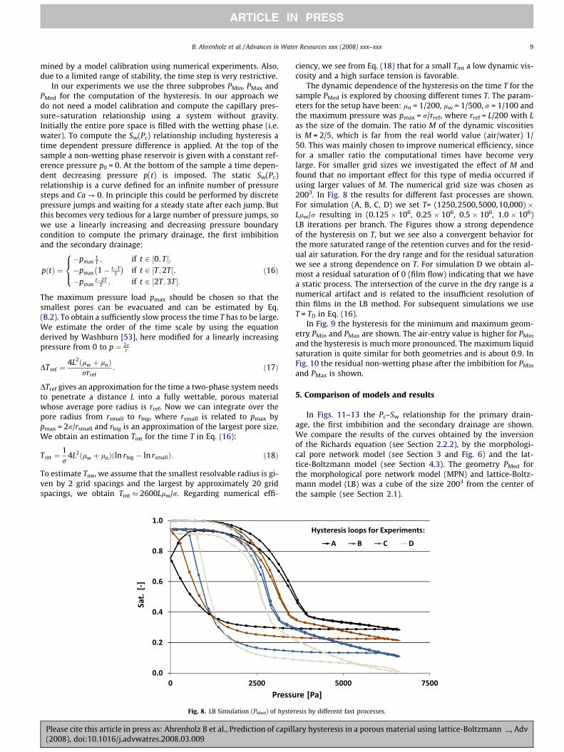
In Fig. 9 the hysteresis for the minimum and maximum geom-etry PMin and PMax are shown. The air-entry value is higher for PMin

and the hysteresis is much more pronounced. The maximum liquidsaturation is quite similar for both geometries and is about 0.9. InFig. 10 the residual non-wetting phase after the imbibition for PMin

and PMax is shown.

5. Comparison of models and results

In Figs. 11–13 the Pc–Sw relationship for the primary drain-age, the first imbibition and the secondary drainage are shown.We compare the results of the curves obtained by the inversionof the Richards equation (see Section 2.2.2), by the morphologi-cal pore network model (see Section 3 and Fig. 6) and the lat-tice-Boltzmann model (see Section 4.3). The geometry PMed forthe morphological pore network model (MPN) and lattice-Boltz-mann model (LB) was a cube of the size 2003 from the center ofthe sample (see Section 2.1).

resis by different fast processes.


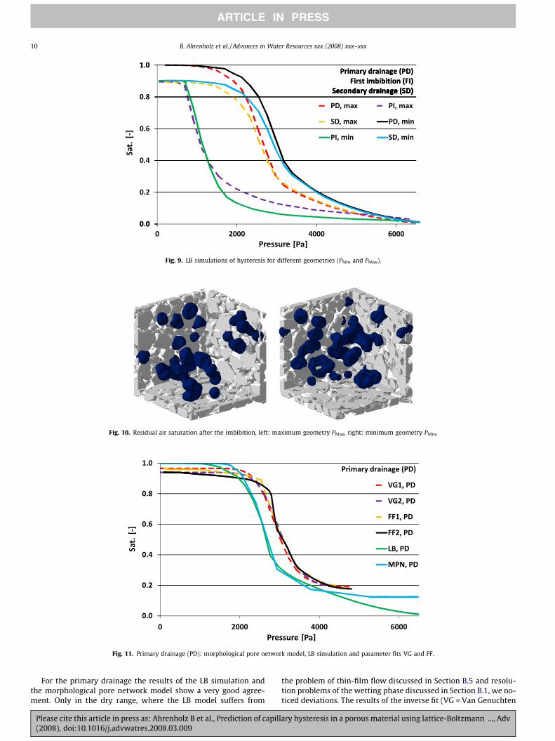
Fig. 11. Primary drainage (PD): morphological pore network model, LB simulation and parameter fits VG and FF.

Fig. 10. Residual air saturation after the imbibition, left: maximum geometry PMax, right: minimum geometry PMin.

Fig. 9. LB simulations of hysteresis for different geometries (PMin and PMax).


ARTICLE IN PRESS

For the primary drainage the results of the LB simulation andthe morphological pore network model show a very good agree-ment. Only in the dry range, where the LB model suffers from


the problem of thin-film flow discussed in Section B.5 and resolu-tion problems of the wetting phase discussed in Section B.1, we no-ticed deviations. The results of the inverse fit (VG = Van Genuchten


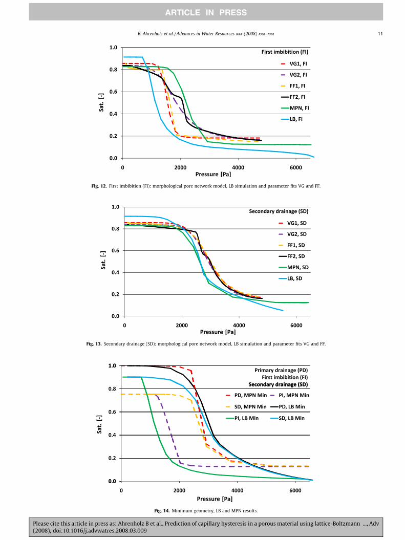
Fig. 14. Minimum geometry, LB and MPN results.

Fig. 12. First imbibition (FI): morphological pore network model, LB simulation and parameter fits VG and FF.

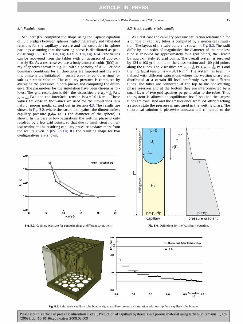
Fig. 13. Secondary drainage (SD): morphological pore network model, LB simulation and parameter fits VG and FF.


ARTICLE IN PRESS

Please cite this article in press as: Ahrenholz B et al., Prediction of capillary hysteresis in a porous material using lattice-Boltzmann ..., Adv(2008), doi:10.1016/j.advwatres.2008.03.009


ARTICLE IN PRESS

constrained, FF = free form) from column 1 and 2 are very similar.They deviate from the results of the LB and MPN methods in ampli-tude by approximately 10%. The value of the slope agrees very well.The residual saturation predicted by the MPN model is 12% and theinverse fit predicts values from 15% to 18%.

For the first imbibition the results by the inverse fit (VG = VanGenuchten constrained, FF = free form) from column 1 and 2 dif-fer. For column 1 we had a very late response leading to a stepfunction for the data FF1 shown in Fig. 12, but the van Genuchtenfit smoothes out this behavior. The results for column 2 aresmoother. Nevertheless the results obtained by either the LB orthe MPN approach show more resemblance to the results fromcolumn 1. In the saturation range between 0.2 and 0.7 the LBand MPN results have a similar slope but the amplitude of the lat-ter is 25% higher. The maximum water content for the wettingprocess is 84–86% for the experimental, 76% for the MPN and90% for the LB results.

For the secondary drainage the results from the LB simulationand the MPN model show a very good agreement in the range ofsaturations between 0.6 and 0.15. In the wetter range the differ-ence is due to the different residual air saturations from the firstimbibition. In the dry range the LB method drains almost com-pletely due to film flow. The results for the inverse fit (VG = VanGenuchten constrained, FF = free form) from column 1 and 2 arevery similar. They deviate from the results of LB and MPN modelin amplitude by approximately 10%. Again the value of the slopeagrees very well.

In Fig. 14 the hysteresis for the minimum geometry, in Fig. 15the hysteresis for the maximum geometry, obtained from the LBsimulation and MPN method are shown. They show good agree-ment for the drainage curves, yet for the imbibition the devia-tions are larger. The air-entry pressure for the minimumgeometry is higher than for the maximum geometry and thisbehavior is reproduced by both models. This can be explainedby the smaller throats of the pore space in the minimum geome-try (small pore width and porosity) that need a higher pressure tobe drained. The maximum water content for the wetting processis approximately 0.9 in both cases for LB and 0.75 (minimumgeometry) and 0.78 (maximum geometry) for the morphologicalpore network model. Referring to the LB results, the hysteretic ef-fect is much more pronounced for the minimum than for themaximum geometry. We observe the same behavior in weakerform for the MPN model as well.

Fig. 15. Maximum geometr


6. Conclusions and outlook

We evaluated the capability of two different multiphase modelsto predict the hysteretic behavior of the capillary pressure satura-tion relationship on the basis of detailed representations of thecomplex porous structure as measured by X-ray tomography. Themodels differ considerably in complexity and computational costsand can have different potential applications. However, the resultsobtained for the primary and secondary drainage curve are consis-tent, while differences among the models for the first imbibitionare observed.

In general MPN models are sufficient to compute the primarydrainage, but the choice of the structural element for imbibition isnot straightforward and changes the results considerably. In contrastthe LB approach needs no modeling (no structural element) for theimbibition, but due to a lack of resolution in the dry range, numericalerrors become large and reliable results are difficult to obtain.

Our work permits the following conclusions:

� The air-entry pressure and the slope of the drainage curves canbe predicted by the LB- and the MPN model very well.

� With the morphological pore network model the residual watersaturation can be predicted, for the LB approach this task is moredifficult due to the limited resolution thin-film flow. In SectionB.5 a method using the LB approach for the prediction of theresidual saturation in a sphere packing is investigated.

� The residual air saturation can be predicted by both models. TheLB model predicts a smaller amount of residual air than the mor-phological pore network model. The experimental results are inbetween.

� In the case of the morphological pore network model, the resultsdepend on the choice of the structural elements to quantify thepore space. While the choice of spheres is reasonable for a drain-age process limited by the smallest curvature radius, the choicefor the wetting process is not straightforward.

� The standard LB approach using uniform grids is limited in thedry range. This is due to the insufficient resolution of thin waterfilms and thus leads to erroneous capillary pressures. One possi-ble solution for the dry range is to use a non-uniform, adaptiveLB approach. Methods for simulations of two-phase flows usingnon-uniform grids have been developed in [1]. Using grid refine-ment for two-phase flow in porous media is a challenge.

y, LB and MPN results.



ARTICLE IN PRESS

� Only with the LB approach it is possible to simulate a fullyresolved simulation of dynamic multiphase phenomena trackingthe interface evolution. Except for the limitation mentionedbefore, the consistency of the results indicates a reliable repre-sentation of the multiphase dynamics.

� The computational costs of LB simulations are orders of magni-tudes higher than for the MPN model, so it is difficult to do asound statistics covering a lot of different geometries with thepresent computational resources.

� Dynamic pore network models can also simulate dynamic phe-nomena, but here some simplifications and assumptions have tobe made which introduce potential modeling errors. For anadvanced network model we refer to [54,55]. One difficulty isto map the pore space to an equivalent pore network represen-tation [16]. On the other hand, the insufficient numerical resolu-tion of the thin-film flow in the LB model in the dry range leadsto numerical errors.

� Comparing to the work of [17] on simulation of hysteresis wecan observe the following common behavior: The amplitude ofthe drainage is approx. 10% below the experimental valuesand the irreducible air saturation is higher than the experimen-tal values. In contrast the amplitude of the first imbibition in oursimulation is below the experimental values, whereas in [17] itis above.

Acknowledgements

The authors would like to thank the Deutsche Forschungsgeme-inschaft (DFG) for supporting this work within the project FIrstPrinciple Based MOdelling of Transport in Unsaturated Media(FIMOTUM) under Grant KR 1747/7-2.

Appendix A. Multiphase lattice-Boltzmann model

The lattice-Boltzmann method is a numerical method to solvethe Navier–Stokes equations [56–58], where density distributionspropagate and collide on a regular lattice. A common labeling fordifferent lattice-Boltzmann models is dxqb [59], where x is thespace dimension and b the number of microscopic velocities. Weuse a three-dimensional nineteen velocity lattice-Boltzmann mod-el (d3q19) for immiscible binary fluids described in [1], which al-lows adjusting the surface tension and the ratio of viscositiesindependently. Here we give a short review of the model optimizedfor Stokes flow. In the following discussion the font bold sans serif(x) represents a three-dimensional vector in space and the fontbold with serif f a b-dimensional vector, where b is the numberof microscopic velocities. The microscopic velocities are given with

fei; i ¼ 0; . . . ;18g ¼0 c �c 0 0 0 0 c �c c �c c �c c �c 0 0 0 00 0 0 c �c 0 0 c �c �c c 0 0 0 0 c �c c �c

0 0 0 0 0 c �c 0 0 0 0 c �c �c c c �c �c c

8><>:9>=>;;

where c is a constant microscopic reference velocity. The micro-scopic velocities define a space-filling computational lattice wherea node is connected to the neighboring nodes through the vectors{Dtei, i = 0, . . . ,18}. The time step Dt defines the grid spacing throughh = cDt. We use two LB schemes: The scheme described in SectionA.1 is used for the advection of two-phase fields indicating the dif-ferent fluid phases. The scheme described in Section A.2 is the flowsolver including the effects of surface tension.


A.1. Lattice-Boltzmann method for the phase field

We introduce a wetting and non-wetting dimensionless densityfield qw and qn and define an order parameter /

/ ¼ qw � qn

qw þ qn; ðA:1Þ

which indicates the fluid phase: / = 1 for the wetting phase and /= �1 for the non-wetting phase. The value of / is constant in the bulkof each phase and varies only in the diffusive fluid–fluid interface.

The gradient C of / is computed by

Cðt; xÞ ¼ 3c2Dt

Xi

wiei/ðt; xþ eiDtÞ: ðA:2Þ

The normalized gradient is

na ¼Ca

j C j ðA:3Þ

and defines the orientation of the fluid–fluid interface.The advection of the density fields w={qw,qn} is done with the

following LB equation:

giðt þ Dt; xþ eiDtÞ ¼ geqi ðwðt; xÞ;uðt; xÞÞ; ðA:4Þ

where gi are dimensionless density distributions. The equilibriumdistribution function geq

i is given by

geqi ðw;uÞ ¼ wiw 1þ 3

c2 ei � u� �

: ðA:5Þ

The velocity u is computed by the flow solver described in SectionA.2. The weights wi are

wi ¼

13 for i ¼ 0;1

18 for i ¼ 1;2;3;4;5;6;1

36 for i ¼ 7;8;9;10;11;12;13;14;15;16;17;18:

8><>: ðA:6Þ

The scheme (A.4) in combination with (A.5) results in an advectiondiffusion equation [60]. The diffusion coefficient is a ¼ 1

6 c2Dt whichis annihilated by the following algorithm: A recoloring step is intro-duced to eliminate the diffusion effects and to achieve a phase sep-aration. The recoloring step redistributes the distributions gi ofphase qr and qb so that the inner product of the gradient C andthe momentum of phase qr is maximized. The constraints are theconservation of the mass of each phase and the conservation ofthe momentum of the sum of both phases. We use the recoloringalgorithm given in [47,40].

Note that for the scheme given by (A.4) we only need the valuew of the phase field and the advection velocity u as input values. So

we need to store only the two variables qr and qb and not the cor-responding nineteen distribution functions for each field.

A.2. Generalized lattice-Boltzmann method for the flow field

We use the generalized lattice-Boltzmann (GLB) equation intro-duced in [61,62] in a modified version [1] and give here a descrip-tion optimized for Stokes flow.



ARTICLE IN PRESS

The lattice-Boltzmann equation is given by

fiðt þ Dt; xþ eiDtÞ ¼ fiðt; xÞ þ Xi; i ¼ 0; . . . ; b� 1; ðA:7Þ

where fi are mass fractions (unit kg m�3) propagating with veloci-ties ei. The collision operator of the multi-relaxation time model(MRT) is given by

X ¼ M�1SððMfÞ �meqÞ: ðA:8ÞThe transformation matrix M

Mi;j ¼ Ui;j; i; j ¼ 0; . . . ; b� 1 ðA:9Þ

is constructed from the orthogonal basis vectors {Ui, i = 0, . . . ,b �1}

U0;a ¼ 1; U1;a ¼ e2a � c2; U2;a ¼ 3ðe2

a Þ2 � 6e2

a c2 þ c4; ðA:10ÞU3;a ¼ eax; U5;a ¼ eay; U7;a ¼ eaz; ðA:11ÞU4;a ¼ ð3e2

a � 5c2Þeax; U6;a ¼ ð3e2a � 5c2Þeay;

U8;a ¼ ð3e2a � 5c2Þeaz; ðA:12Þ

U9;a ¼ 3e2ax � e2

a ; U11;a ¼ e2ay � e2

az; ðA:13ÞU13;a ¼ eaxeay; U14;a ¼ eayeaz; U15;a ¼ eaxeaz; ðA:14ÞU10;a ¼ ð2e2

a � 3c2Þð3e2ax � e2

aÞ; U12;a ¼ ð2e2a � 3c2Þðe2

ay � e2azÞ;ðA:15Þ

U16;a ¼ ðe2ay � e2

azÞeax; U17;a ¼ ðe2az � e2

axÞeay;

U18;a ¼ ðe2ax � e2

ayÞeaz ðA:16Þ

and transforms the distributions into moment space. In Appendix Cthe matrix is given in full detail. The resulting moments m = Mf arelabeled as

m ¼ ðdq; e; n; q0ux; qx; q0uy; qy; q0uz; qz; pxx; pxx; pww; pww; pxy; pyz; pxz;

mx;my;mzÞ; ðA:17Þ

where dq is a density variation, j = q0 (ux,uy,uz) is the momentum, q0

is a constant reference density and u=(ux,uy,uz) is the velocity vec-tor. The moments e, pxx, pww, pxy, pyz, pxz of second order are relatedto the strain rate tensor. The other moments of higher order are re-lated to higher order derivatives of the flow field and have no directphysical impact with respect to the incompressible Navier–Stokesequations.

The vector meq is composed of the equilibrium moments ex-tended by terms responsible for the generation of surface tensionand is given by

meq0 ¼ dq; ðA:18aÞ

meq1 ¼ eeq ¼ �r j C j; ðA:18bÞ

meq3 ¼ q0ux; ðA:18cÞ

meq5 ¼ q0uy; ðA:18dÞ

meq7 ¼ q0uz; ðA:18eÞ

meq9 ¼ 3peq

xx ¼12

r j C j ð2n2x � n2

y � n2z Þ; ðA:18fÞ

meq11 ¼ peq

zz ¼12

r j C j ðn2y � n2

z Þ; ðA:18gÞ

meq13 ¼ peq

xy ¼12

r j C j ðnxnyÞ; ðA:18hÞ

Fig. B.1. Pendular rings between solids at different saturations in a BCC array


meq14 ¼ peq

yz ¼12

r j C j ðnynzÞ; ðA:18iÞ

meq15 ¼ peq

xz ¼12

r j C j ðnxnzÞ; ðA:18jÞ

meq2 ¼ meq

4 ¼ meq6 ¼ meq

8 ¼ meq16 ¼ meq

17 ¼ meq18 ¼ 0: ðA:18kÞ

The definitions of C and n are given in Eqs. (A.2) and (A.3).The moments {mk, k = 0,3,5,7} are conserved during the colli-

sion, leading to mass and momentum conservation of the algorithm.The matrix S is a diagonal collision matrix composed of relaxationrates {si,i, i = 1, . . . ,b�1}, also called the eigenvalues of the collisionmatrix M�1SM. The rates which are different from zero are

s1;1 ¼ �se;

s2;2 ¼ �sn;

s4;4 ¼ s6;6 ¼ s8;8 ¼ �sq;

s10;10 ¼ s12;12 ¼ �sp;

s9;9 ¼ s11;11 ¼ s13;13 ¼ s14;14 ¼ s15;15 ¼ �sm;

s16;16 ¼ s17;17 ¼ s18;18 ¼ �sm:

The relaxation rate sm is related to the kinematic viscosity m by

1sm¼ 3

mc2Dt

þ 12: ðA:19Þ

The other relaxation rates se, sn, sq, sp and sm can be freely chosen inthe range [0,2] and may be tuned to improve accuracy and/or sta-bility [62]. The optimal values depend on the specific system underconsideration (geometry, initial and boundary conditions) and can-not be computed in advance for general cases. For Stokes flow agood choice are the ‘‘magic” parameters relaxing the even and theodd moments differently [63]:

se ¼ sn ¼ sp ¼ sm; sq ¼ sm ¼ 8ð2� smÞð8� smÞ

: ðA:20Þ

The pressure variation dp is given by

dp ¼ c2

3dq: ðA:21Þ

A detailed mathematical analysis shows that this numerical modelyields the Navier–Stokes equation for two immiscible phases withsurface tension [60] (for single-phase flow see [56,64]). The schemeis formally first order in time and second order in space. Note thatthe extensions to the original method [34], especially the linearadvection scheme, the moment method and the altered terms(A.18b)–(A.18k) for imposing surface tension, substantially improvethe numerical efficiency. A method for adjusting the contact anglebetween the wetting and non-wetting phase is proposed in [40].

Appendix B. Validation of the lattice-Boltzmann model

Different validation examples have been set up to test and ex-plore the LB method proposed here for the simulation of multi-phase flow problems in porous media.

of spheres. Left: plain geometry, middle and right: computational results.



ARTICLE IN PRESS

B.1. Pendular rings

Schubert [65] computed the shape using the Laplace equationof fluid bridges between spheres neglecting gravity and tabulatedrelations for the capillary pressure and the saturation in spherepackings assuming that the wetting phase is distributed as pen-dular rings [65, see p. 128, Fig. 4.12; p. 138, Fig. 4.24]. The valuescan be recovered from the tables with an accuracy of approxi-mately 5%. As a test case we use a body centered cubic (BCC) ar-ray of spheres shown in Fig. B.1 with a porosity of 0.32. Periodicboundary conditions for all directions are imposed and the wet-ting phase is pre-initialized in such a way that pendular rings re-sult as a static solution. The capillary pressure is computed byaveraging the pressures in both phases and computing the differ-ence. The parameters for the simulation have been chosen as fol-lows: The grid resolution is 963, the viscosities are lw ¼ 1

60 Pa s,ln ¼ 1

600 Pa s and the interfacial tension is r = 0.01 N m�1. Thesevalues are close to the values we used for the simulations in anatural porous media carried out in Section 4.3. The results areshown in Fig. B.2, where the saturation against the dimensionlesscapillary pressure pcd/r (d is the diameter of the sphere) isshown. In the case of low saturations the wetting phase is onlyresolved by a few grid points, so that due to insufficient numer-ical resolution the resulting capillary pressure deviates more fromthe results given in [65]. In Fig. B.1 the resulting shape for twoconfigurations are shown.

Fig. B.3. Left: static capillary tube bundle, right: capillary pres

Fig. B.2. Capillary pressure for pendular rings at different saturations.


B.2. Static capillary tube bundle

As a test case the capillary pressure saturation relationship fora bundle of capillary tubes is computed by a numerical simula-tion. The layout of the tube bundle is shown in Fig. B.3. The radiidiffer by one order of magnitude; the diameter of the smallesttube is resolved by approximately four grid points, the largestby approximately 20 grid points. The overall system is resolvedby 124 � 108 grid points in the cross-section and 100 grid pointsalong the tubes. The viscosities are lw ¼ 1

60 Pa s, ln ¼ 1600 Pa s and

the interfacial tension is r = 0.01 N m�1. The system has been ini-tialized with different saturations where the wetting phase wasdistributed at a certain fill level uniformly over the differenttubes. The tubes are connected at the top to the non-wettingphase reservoir and at the bottom they are interconnected by asmall layer of two grid spacings perpendicular to the tubes. Thusthe system is allowed to equilibrate itself, so that the largesttubes are evacuated and the smaller ones are filled. After reachinga steady state the pressure is measured in the wetting phase. Thetheoretical solution is piecewise constant and compared to the

sure – saturation relationship for a capillary tube bundle.

Fig. B.4. Definitions for the Washburn equation.


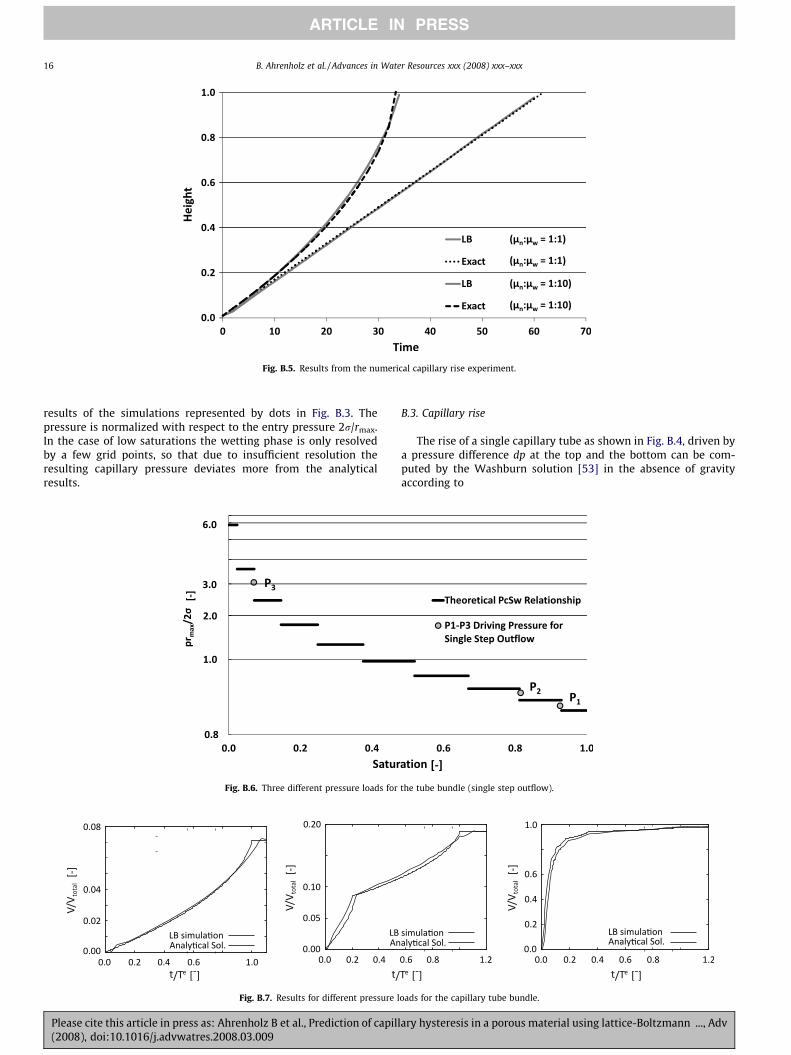
Fig. B.5. Results from the numerical capillary rise experiment.


ARTICLE IN PRESS

results of the simulations represented by dots in Fig. B.3. Thepressure is normalized with respect to the entry pressure 2r/rmax.In the case of low saturations the wetting phase is only resolvedby a few grid points, so that due to insufficient resolution theresulting capillary pressure deviates more from the analyticalresults.

Fig. B.6. Three different pressure loads for

Fig. B.7. Results for different pressure l


B.3. Capillary rise

The rise of a single capillary tube as shown in Fig. B.4, driven bya pressure difference dp at the top and the bottom can be com-puted by the Washburn solution [53] in the absence of gravityaccording to

the tube bundle (single step outflow).

oads for the capillary tube bundle.


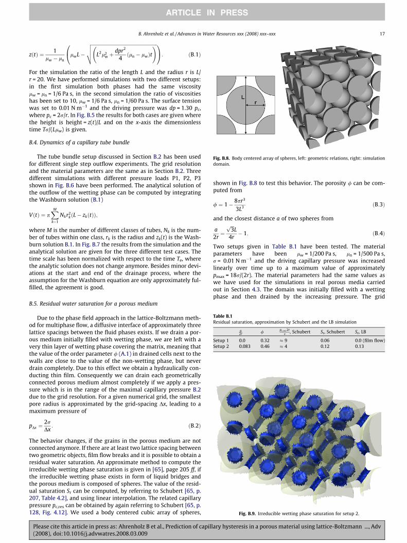
Fig. B.8. Body centered array of spheres, left: geometric relations, right: simulationdomain.

Table B.1Residual saturation, approximation by Schubert and the LB simulation

a2r /

pc;res 2rr , Schubert Sr, Schubert Sr, LB

Setup 1 0.0 0.32 � 9 0.06 0.0 (film flow)Setup 2 0.083 0.46 � 4 0.12 0.13

Fig. B.9. Irreducible wetting phase saturation for setup 2.


ARTICLE IN PRESS

zðtÞ ¼ 1lw � ln

lwL�

ffiffiffiffiffiffiffiffiffiffiffiffiffiffiffiffiffiffiffiffiffiffiffiffiffiffiffiffiffiffiffiffiffiffiffiffiffiffiffiffiffiffiffiffiffiffiffiffiffiffiffiffiffiffiffiffiL2l2

w þdpr2

4ðln � lwÞt

!vuut0@ 1A: ðB:1Þ

For the simulation the ratio of the length L and the radius r is L/r = 20. We have performed simulations with two different setups:in the first simulation both phases had the same viscositylw = ln = 1/6 Pa s, in the second simulation the ratio of viscositieshas been set to 10, lw = 1/6 Pa s, ln = 1/60 Pa s. The surface tensionwas set to 0.01 N m�1 and the driving pressure was dp = 1.30 pc,where pc = 2r/r. In Fig. B.5 the results for both cases are given wherethe height is height = z(t)/L and on the x-axis the dimensionlesstime Tr/(Llw) is given.

B.4. Dynamics of a capillary tube bundle

The tube bundle setup discussed in Section B.2 has been usedfor different single step outflow experiments. The grid resolutionand the material parameters are the same as in Section B.2. Threedifferent simulations with different pressure loads P1, P2, P3shown in Fig. B.6 have been performed. The analytical solution ofthe outflow of the wetting phase can be computed by integratingthe Washburn solution (B.1)

VðtÞ ¼ pXM

k¼1

Nkr2kðL� zkðtÞÞ;

where M is the number of different classes of tubes, Nk is the num-ber of tubes within one class, rk is the radius and zk(t) is the Wash-burn solution B.1. In Fig. B.7 the results from the simulation and theanalytical solution are given for the three different test cases. Thetime scale has been normalized with respect to the time Te, wherethe analytic solution does not change anymore. Besides minor devi-ations at the start and end of the drainage process, where theassumption for the Washburn equation are only approximately ful-filled, the agreement is good.

B.5. Residual water saturation for a porous medium

Due to the phase field approach in the lattice-Boltzmann meth-od for multiphase flow, a diffusive interface of approximately threelattice spacings between the fluid phases exists. If we drain a por-ous medium initially filled with wetting phase, we are left with avery thin layer of wetting phase covering the matrix, meaning thatthe value of the order parameter / (A.1) in drained cells next to thewalls are close to the value of the non-wetting phase, but neverdrain completely. Due to this effect we obtain a hydraulically con-ducting thin film. Consequently we can drain each geometricallyconnected porous medium almost completely if we apply a pres-sure which is in the range of the maximal capillary pressure B.2due to the grid resolution. For a given numerical grid, the smallestpore radius is approximated by the grid-spacing Dx, leading to amaximum pressure of

pDx ¼2rDx

: ðB:2Þ

The behavior changes, if the grains in the porous medium are notconnected anymore. If there are at least two lattice spacing betweentwo geometric objects, film flow breaks and it is possible to obtain aresidual water saturation. An approximate method to compute theirreducible wetting phase saturation is given in [65], page 205 ff, ifthe irreducible wetting phase exists in form of liquid bridges andthe porous medium is composed of spheres. The value of the resid-ual saturation Sr can be computed, by referring to Schubert [65, p.207, Table 4.2], and using linear interpolation. The related capillarypressure pc,res can be obtained by again referring to Schubert [65, p.128, Fig. 4.12]. We used a body centered cubic array of spheres,


shown in Fig. B.8 to test this behavior. The porosity / can be com-puted from

/ ¼ 1� 8pr3

3L3 ðB:3Þ

and the closest distance a of two spheres from

a2r¼

ffiffiffi3p

L4r� 1: ðB:4Þ

Two setups given in Table B.1 have been tested. The materialparameters have been lw = 1/200 Pa s, ln = 1/500 Pa s,r = 0.01 N m�1 and the driving capillary pressure was increasedlinearly over time up to a maximum value of approximatelypmax = 18r/(2r). The material parameters had the same values aswe have used for the simulations in real porous media carriedout in Section 4.3. The domain was initially filled with a wettingphase and then drained by the increasing pressure. The grid



ARTICLE IN PRESS

resolution was 1503, so that one sphere is resolved by approxi-mately 40 grid points. In the first case the medium is drained al-most completely, whereas in the second case we obtain a residualsaturation of 0.13. The distribution of the non-wetting phase(NWP) is shown in Fig. B.9. The values of setup 2 are very closeand indicate the validity of the approach. Nevertheless furtherinvestigation has to be done and is beyond the scope of thispaper.

For a general porous medium obtained by tomography methodsit is very difficult to estimate the irreducible NWP saturation bylattice Boltzmann methods, since the medium is generally con-nected and the individual grains are not known. A method to iden-

M ¼

1� ð1 1 1 1 1 1 1 1 1 1 1 1c2� ð�1 0 0 0 0 0 0 1 1 1 1 1c4� ð1 �2 �2 �2 �2 �2 �2 1 1 1 1 1c� ð0 1 �1 0 0 0 0 1 �1 1 �1 1c3� ð0 �2 2 0 0 0 0 1 �1 1 �1 1c� ð0 0 0 1 �1 0 0 1 �1 �1 1 0c3� ð0 0 0 �2 2 0 0 1 �1 �1 1 0c� ð0 0 0 0 0 1 �1 0 0 0 0 1c3� ð0 0 0 0 0 �2 2 0 0 0 0 1c2� ð0 2 2 �1 �1 �1 �1 1 1 1 1 1c4� ð0 �2 �2 1 1 1 1 1 1 1 1 1c2� ð0 0 0 1 1 �1 �1 1 1 1 1 �1c4� ð0 0 0 �1 �1 1 1 1 1 1 1 �1c2� ð0 0 0 0 0 0 0 1 1 �1 �1 0c2� ð0 0 0 0 0 0 0 0 0 0 0 0c2� ð0 0 0 0 0 0 0 0 0 0 0 1c3� ð0 0 0 0 0 0 0 1 �1 1 �1 �1c3� ð0 0 0 0 0 0 0 �1 1 1 �1 0c3� ð0 0 0 0 0 0 0 0 0 0 0 1

2666666666666666666666666666666666666666664

Table D.1Estimated parameters for the primary drainage branch – column 1/2

Parameter Unit

qb kg m�3

/a –Ks m2

hs –

Estimated

vG cons vG unco

a1 Pa�1 3.39E�04/3.34E�04 3.64E�0n1 – 11.42/10.91 15.13/11m1 – =1 � 1/n1 0.479/0.8hr – 0.076/0.070 0.070/0.0a2 Pa�1 – –n2 – – –m2 – – –w2 – – –s – 0.625/0.370 1.039/0.4

RMSEpb Pa 5.86E+01/2.68E+01 5.64E+01

RMSEQc m 4.18E�04/3.53E�04 3.95E�0

a Calculated assuming qs = 2650 kg m�3: / = 1 � qb/qs.b Root mean square error of the measurement and model prediction of capillary presc Root mean square error of the measurement and model prediction of cumulative ou


tify single items in the structure is described in [22]. A possiblefuture direction to estimate the irreducible NWP saturation by LBmethods could use these methods and shrink the single items bytwo voxel layers in the numerical simulation grid. Finally one hasto do several simulation runs on successively refined grids, alwayskeeping a distance of two voxel layers between the single items,until a convergent behavior is observed. Nevertheless this is a verydemanding simulation setup.

Appendix C. Transformation matrix M

1 1 1 1 1 1 1Þ1 1 1 1 1 1 1Þ1 1 1 1 1 1 1Þ�1 1 �1 0 0 0 0Þ�1 1 �1 0 0 0 0Þ0 0 0 1 �1 1 �1Þ0 0 0 1 �1 1 �1Þ�1 �1 1 1 �1 �1 1Þ�1 �1 1 1 �1 �1 1Þ1 1 1 �2 �2 �2 �2Þ1 1 1 �2 �2 �2 �2Þ�1 �1 �1 0 0 0 0Þ�1 �1 �1 0 0 0 0Þ0 0 0 0 0 0 0Þ0 0 0 1 1 �1 �1Þ1 �1 �1 0 0 0 0Þ1 �1 1 0 0 0 0Þ0 0 0 1 �1 1 �1Þ�1 �1 1 �1 1 1 �1Þ

3777777777777777777777777777777777777777775

Measured

1567/15630.409/0.4104.09E�11/1.94E�110.396/0.385

ns vG bimod ff

4/3.36E�04 3.37E�04/3.31E�04 –.05 12.77/12.04 –70 =1 � 1/n1 –70 0.072/0.073 –

7.77E�04/1.09E�03 –1.87/4.93 –=1 � 1/n2 –0.061/0.032 –

08 0.902/0.216 –

/2.67E+01 5.73E+01/2.83E+01 5.66E+01/3.20E+014/3.53E�04 3.42E�04/2.21E�04 2.04E�04/7.56E�05

sure, p.tflow, Q.



ARTICLE IN PRESS

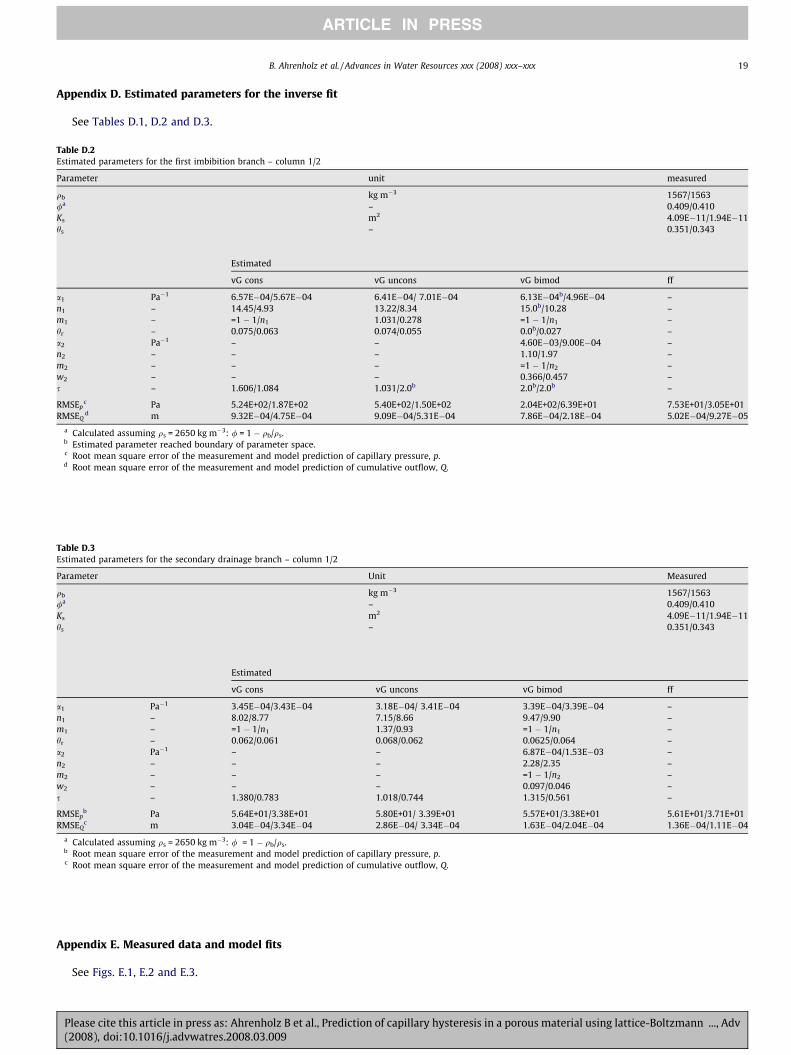
Appendix D. Estimated parameters for the inverse fit

See Tables D.1, D.2 and D.3.

Table D.2Estimated parameters for the first imbibition branch – column 1/2

Parameter unit measured

qb kg m�3 1567/1563/a – 0.409/0.410Ks m2 4.09E�11/1.94E�11hs – 0.351/0.343

Estimated

vG cons vG uncons vG bimod ff

a1 Pa�1 6.57E�04/5.67E�04 6.41E�04/ 7.01E�04 6.13E�04b/4.96E�04 –n1 – 14.45/4.93 13.22/8.34 15.0b/10.28 –m1 – =1 � 1/n1 1.031/0.278 =1 � 1/n1 –hr – 0.075/0.063 0.074/0.055 0.0b/0.027 –a2 Pa�1 – – 4.60E�03/9.00E�04 –n2 – – – 1.10/1.97 –m2 – – – =1 � 1/n2 –w2 – – – 0.366/0.457 –s – 1.606/1.084 1.031/2.0b 2.0b/2.0b –

RMSEpc Pa 5.24E+02/1.87E+02 5.40E+02/1.50E+02 2.04E+02/6.39E+01 7.53E+01/3.05E+01

RMSEQd m 9.32E�04/4.75E�04 9.09E�04/5.31E�04 7.86E�04/2.18E�04 5.02E�04/9.27E�05

a Calculated assuming qs = 2650 kg m�3: / = 1 � qb/qs.b Estimated parameter reached boundary of parameter space.c Root mean square error of the measurement and model prediction of capillary pressure, p.d Root mean square error of the measurement and model prediction of cumulative outflow, Q.

Table D.3Estimated parameters for the secondary drainage branch – column 1/2

Parameter Unit Measured

qb kg m�3 1567/1563/a – 0.409/0.410Ks m2 4.09E�11/1.94E�11hs – 0.351/0.343

Estimated

vG cons vG uncons vG bimod ff

a1 Pa�1 3.45E�04/3.43E�04 3.18E�04/ 3.41E�04 3.39E�04/3.39E�04 –n1 – 8.02/8.77 7.15/8.66 9.47/9.90 –m1 – =1 � 1/n1 1.37/0.93 =1 � 1/n1 –hr – 0.062/0.061 0.068/0.062 0.0625/0.064 –a2 Pa�1 – – 6.87E�04/1.53E�03 –n2 – – – 2.28/2.35 –m2 – – – =1 � 1/n2 –w2 – – – 0.097/0.046 –s – 1.380/0.783 1.018/0.744 1.315/0.561 –

RMSEpb Pa 5.64E+01/3.38E+01 5.80E+01/ 3.39E+01 5.57E+01/3.38E+01 5.61E+01/3.71E+01

RMSEQc m 3.04E�04/3.34E�04 2.86E�04/ 3.34E�04 1.63E�04/2.04E�04 1.36E�04/1.11E�04

a Calculated assuming qs = 2650 kg m�3: / = 1 � qb/qs.b Root mean square error of the measurement and model prediction of capillary pressure, p.c Root mean square error of the measurement and model prediction of cumulative outflow, Q.

Appendix E. Measured data and model fits

See Figs. E.1, E.2 and E.3.


0 0.5 1 1.5 2 2.5 3 3.5 4x 105

−5000

−4000

−3000

−2000

−1000

0

pres

sure

[Pa]

0 0.5 1 1.5 2 2.5 3 3.5 4x 105

0

0.005

0.01

0.015

0.02

0.025

cum

ulat

ive

outfl

ow [m

]

time [sec]

measuredvG consvG unconsvG bimodfree formlower boundary

pressure

outflow

0 0.5 1 1.5 2 2.5 3 3.5 4x 105

−5000

−4000

−3000

−2000

−1000

0

pres

sure

[Pa]

0 0.5 1 1.5 2 2.5 3 3.5 45

0

0.005

0.01

0.015

0.02

0.025

cum

ulat

ive

outfl

ow [m

]

time [sec]


pressure

outflow

0 1 2 3 4 5x 104

0

0.002

0.004

0.006

0.008

0.01

cum

ulat

ive

outfl

ow [m

]

time [sec]0 1 2 3 4 5

x 104time [sec]


0

0.002

0.004

0.006

0.008

0.01

cum

ulat

ive

outfl

ow [m

]


Fig. E.1. Primary drainage branch: measured data and fitted with four different hydraulic properties models. Top: matric head and cumulative outflow for column 1; Middle:matric head and cumulative outflow for column 2; Bottom: cumulative outflow for column 1 (left) and 2 (right) for hLB P �25 to show the better performance of the moreflexible models.


ARTICLE IN PRESS

Please cite this article in press as: Ahrenholz B et al., Prediction of capillary hysteresis in a porous material using lattice-Boltzmann ..., Ad(2008), doi:10.1016/j.advwatres.2008.03.009

v

0 0.5 1 1.5 2 2.5 3 3.5 4x 105

−5000

−4000

−3000

−2000

−1000

0

pres

sure

[Pa]

pres

sure

[Pa]

0 0.5 1 1.5 2 2.5 3 3.5 4x 105

−0.02

−0.015

−0.01

−0.005

0

cum

ulat

ive

outfl

ow [m

]

time [sec]


pressure

outflow

0 0.5 1 1.5 2 2.5 3 3.5x 105

−5000

−4000

−3000

−2000

−1000

0

0 0.5 1 1.5 2 2.5 3 3.5x 105

−0.02

−0.015

−0.01

−0.005

0

cum

ulat

ive

outfl

ow [m

]time [sec]


pressure

outflow

2.8 3 3.2 3.4x 105

-0.024

-0.02

-0.016

-0.012

-0.008

-0.004

0

cum

ulat

ive

outfl

ow [m

]

time [sec]


Fig. E.2. First imbibition branch: measured data and fitted with four different hydraulic properties models. Top: matric head and cumulative outflow for column 1; middle:matric head and Cumulative outflow for column 2; bottom: cumulative outflow for column 2 for hLB P �25 to show the better performance of the more flexible models.


ARTICLE IN PRESS


0 0.5 1 1.5 2 2.5 3 3.5 4

x 105

−5000

−4000

−3000

−2000

−1000

0

pres

sure

[Pa]

0 0.5 1 1.5 2 2.5 3 3.5 4

x 105

0

0.005

0.01

0.015

0.02

cum

ulat

ive

outfl

ow [m

]

time [sec]


pressure

outflow

0 0.5 1 1.5 2 2.5 3 3.5 4

x 105

−5000

−4000

−3000

−2000

−1000

0

pres

sure

[Pa]

0 0.5 1 1.5 2 2.5 3 3.5 4

x 105

0

0.005

0.01

0.015

0.02

cum

ulat

ive

outfl

ow [m

]time [sec]


pressure

outflow

0 1 2 3 4 5

x 104

0

0.002

0.004

0.006

0.008

0.01

cum

ulat

ive

outfl

ow [m

]

time [sec]0 1 2 3 4 5

x 104time [sec]


0

0.002

0.004

0.006

0.008

0.01

cum

ulat

ive

outfl

ow [m

]


Fig. E.3. Secondary drainage branch: Measured data and fitted with four different hydraulic properties models. Top: matric head and cumulative outflow for column 1;middle: matric head and cumulative outflow for column 2; bottom: cumulative outflow for column 1 (left) and 2 (right) hLB P �25 to show the better performance of themore flexible models.


ARTICLE IN PRESS

References

[1] Tölke J, Freudiger S, Krafczyk M. An adaptive scheme for LBE multiphase flowsimulations on hierarchical grids. Comput Fluids 2006;35:820–30.

[2] Haines W. Studies in the physical properties of soils: V. The hysteresis effect incapillary properties, and the modes of moisture distribution associatedtherewith. J Agri Sci 1930;20:97–116.


[3] Moseley W, Dhir VK. Capillary pressure–saturation relationship in porousmedia including the effect of wettability. J Hydrol 1996;178:33–53.

[4] Lehmann P, Stauffer F, Hinz C, Dury O, Flühler H. Effect of hysteresis on waterflow in sand column with a fluctuating capillary fringe. J Contam Hydrol1998;33:81–100.

[5] Russo D, Jury W, Butters G. Numerical analysis of solute transport duringtransient irrigation: 1. The effect of hysteresis and profile heterogeneity. WaterResource Res 1989;25:2109–18.



ARTICLE IN PRESS

[6] Mualem Y. A conceptual model of hysteresis. Water Resour Res1974;10:514–20.

[7] Kool J, Parker J. Development and evaluation of closed-form expressions forhysteretic soil hydraulic properties. Water Resour Res 1987;23:105–14.

[8] Huang H-C, Tan Y-C, Liu C-W, Chen C-H. A novel hysteresis model inunsaturated soils. Hydrol Process 2005;19:1653–65.

[9] Mualem Y. Extension of the similarity hypothesis used for modeling soil watercharacteristics. Water Resour Res 1977;13:773–80.

[10] O’Kane J, Flynn D. Thresholds switches and hysteresis in hydrology from thepedon to the catchment scale: a non-linear systems theory. Hydrol Earth SystSci 2007;11:443–59.

[11] Hilfer R. Macroscopic capillarity and hysteresis for flow in porous media. PhysRev E 2006;73:016307.

[12] Jerauld G, Salter S. The effect of pore-structure on hysteresis in relativepermeability and capillary pressure: pore-level modeling. Transp PorousMedia 1989;5:103–51.

[13] Held R, Celia M. Modeling support of functional relationships betweencapillary pressure, saturation, interfacial area and common lines. Adv WaterRes 2001;24:325–43.

[14] Vidales A, Faccio R, Zgrablich G. Capillary hysteresis in porous media. J Phys:Cond Mat 1995;7:3835–43.

[15] Øren P-E, Bakke S, Arntzen OJ. Extending predictive capabilities to networkmodels. SPE J 1998;3:324–36.

[16] Valvatne P, Piri M, Lopez X, Blunt M. Predictive pore-scale modeling of singleand multiphase flow. Transp Porous Media 2005;58:23–41.

[17] Pan C, Hilpert M, Miller CT. Lattice-Boltzmann simulation of two-phase flow inporous media. Water Resour Res 2004;40:W01501.

[18] Shan X, Chen H. Lattice Boltzmann model for simulating flows with multiplephases and components. Phys Rev E 1993;47:1815–9.

[19] Li H, Pan C, Miller C. Pore-scale investigation of viscous coupling effects fortwo-phase flow in porous media. Phys Rev E 2005;72:026705.

[20] Vogel H-J, Tölke J, Schulz VP, Krafczyk M, Roth K. Comparison of a lattice-Boltzmann model, a full-morphology model, and a pore network model fordetermining capillary pressure–saturation relationships. Vadose Zone J2005;4(2):380–8.

[21] Ahrenholz B, Tölke J, Krafczyk M. Lattice-Boltzmann simulations inreconstructed parametrized porous media. Int J Comput Fluid Dyn2006;20(6):369–77.

[22] A. Kaestner, E. Lehmann, M. Stampanoni, Imaging and image processing in soilscience, Adv Water Res, this issue, doi:10.1016/j.advwatres.2008.01.022.

[23] Zurmühl T. Capability of convection dispersion transport models to predicttransient water and solute movement in undisturbed soil columns. J ContamHydrol 1998;30:99–126.

[24] van Genuchten MT. A closed-form equation for predicting the hydraulicconductivity of unsaturated soils. Soil Sci Soc Am J 1980;44:892–8.

[25] Durner W. Hydraulic conductivity estimation for soils with heterogeneouspore structure. Water Resour Res 1994;30:211–23.

[26] Bitterlich S, Durner W, Iden SC, Knabner P. Inverse estimation of theunsaturated soil hydraulic properties from column outflow experimentsusing free-form parameterizations. Vadose Zone J 2004;3:971–81.

[27] Mualem Y. A new model for predicting the hydraulic conductivity ofunsaturated porous media. Water Resour Res 1976;12(3):513–21.

[28] Priesack E, Durner W. Closed form expression for the multi-modal unsaturatedconductivity function. Vadose Zone J 2006;5:121–4.

[29] Duan Q, Sorooshian S, Gupta V. Effective and efficient global optimization forconceptual rainfall-runoff models. Water Resour Res 1992;28:1015–31.

[30] Peters A, Durner W. Improved estimation of soil water retentioncharacteristics from hydrostatic column experiments. Water Resour Res2006;42(11):W11401.

[31] Hilpert M, Miller C. Pore-morphology-based simulation of drainage in totallywetting porous media. Adv Water Res 2001:243–55.

[32] Lehmann P, Wyss P, Flisch A, Lehmann E, Vontobel P, Krafczyk M, et al.Tomographical imaging and mathematical description of porous media usedfor the prediction of fluid distribution. Vadose Zone J 2006;5:80–97.

[33] Rothmann DH, Keller JM. Immiscible cellular automaton fluids. J Stat Phys1988;52:1119–27.

[34] Gunstensen A, Rothman D. Lattice Boltzmann model of immiscible fluids. PhysRev A 1991;43(8):4320–7.

[35] Grunau D, Chen S, Eggert K. A lattice Boltzmann model for multiphase fluidflows. Phys Fluids A: Fluid Dyn 1993;5(10):2557–62.


[36] Swift MR, Osborn WR, Yeomans JM. Lattice Boltzmann Simulation of NonidealFluids. Phys Rev Lett 1995;75(5):830–3.

[37] Luo L-S. Unified theory of the lattice Boltzmann models for nonideal gases.Phys Rev Lett 1998;81(8):1618–21.

[38] Bouzidi M, Firdaouss M, Lallemand P. Momentum transfer of a Boltzmann-Lattice fluid with boundaries. Phys Fluids 2001;13(11):3452–9.

[39] Lallemand P, Luo L-S. Lattice Boltzmann method for moving boundaries. JComput Phys 2003;184:406–21.

[40] Tölke J. Gitter–Boltzmann–Verfahren zur Simulation vonZweiphasenströmungen, PhD thesis, TU München; 2001.

[41] MPI-Forum, Message passing interface; 2006. <http://www.mpi-forum.org>.[42] Lewiner T, Lopes H, Vieira AW, Tavares G. Efficient implementation of

Marching Cubes’ cases with topological guarantees. J Graph Tools2003;8(2):1–15.

[43] Kozeny J. Über kapillare Leitung des Wassers im Boden – Aufstieg,Versickerung und Anwendung auf die Bewässerung, SitzungsberichteAkademie der Wissenschaften Wien. Abt IIa 1927;136:271–306.

[44] Martys N, Chen H. Simulation of multicomponent fluids in complex three-dimensional geometries by the lattice Boltzmann method. Phys Rev E1996;53:743–50.

[45] Adler PM, Thovert FF. Real porous media: local geometry and macroscopicproperties. Appl Mech Rev 1998;51(9):537–85.

[46] Yang ZL, Dinh TN, Nourgaliev RR, Sehgal BR. Evaluation of the Darcys lawperformance for two-fluid flow hydrodynamics in a particle debris bed using alattice-Boltzmann model. Heat Mass Transfer 2000;36:295–304.

[47] Tölke J, Krafczyk M, Schulz M, Rank E. Lattice Boltzmann simulations of binaryfluid flow through porous media. Phil Trans Royal Soc A – Math, Phys Eng Sci2002;360(1792):573–91.

[48] Bekri S, Vizikab O, Thovert J-F, Adler P. Binary two-phase flow with phasechange in porous media. Int J Multiphase Flow 2001;27:477–526.

[49] Adler PM, Thovert J-F, Bekri S, Yousefian F. Real porous media: local geometryand transports. J Eng Mech (ASCE) 2002;128(8):829–39.

[50] Bekri S, Adler PM. Dispersion in multiphase flow through porous media. Int JMultiphase Flow 2002;28:665–97.

[51] Bekri S, Howard J, Muller J, Adler PM. Electrical resistivity index in multiphaseflow through porous media. Transp Porous Media 2003;51(1):41–65.

[52] Lehmann P, Krafczyk M, Gygi A, Flisch A, Wyss P, Flühler H. Modelling flow ofwater and air in reconstructed structures of porous media. In: Proceedings ofthe second world congress on industrial tomography, Hannover; 2001. p. 628–35.

[53] Washburn EW. The dynamics of capillary flow. Phys Rev 1921;17(3):273–83.[54] Piri M, Blunt MJ. Three-dimensional mixed-wet random pore-scale network

modeling of two- and three-phase flow in porous media. I. Model description.Phys Rev E 2005;71:026301.

[55] Piri M, Blunt MJ. Three-dimensional mixed-wet random pore-scale networkmodeling of two- and three-phase flow in porous media. II. Results. Phys Rev E2005;71:026302.

[56] Frisch U, d’HumiFres D, Hasslacher B, Lallemand P, Pomeau Y, Rivet J-P. Latticegas hydrodynamics in two and three dimensions. Comp Syst 1987:75–136.

[57] Benzi R, Succi S, Vergassola M. The lattice Boltzmann equation: theory andapplications. Phys Rep 1992;222(3):147–97.

[58] Chen S, Doolen G. Lattice Boltzmann method for fluid flows. Annu Rev FluidMech 1998;30:329–64.

[59] Qian YH, d’Humières D, Lallemand P. Lattice BGK models for Navier–Stokesequation. Europhys Lett 1992;17:479–84.

[60] Kehrwald D. Numerical analysis of immiscible lattice BGK, PhD thesis,Universität Kaiserslautern; 2003.

[61] d’Humières D. Generalized lattice-Boltzmann equations. in: Shizgal BD, WeaveDP, editors, Rarefied gas dynamics: theory and simulations, Prog AstronautAeronaut, vol. 159. AIAA, Washington DC; 1992. p. 450–58.

[62] Lallemand P, Luo L-S. Theory of the lattice Boltzmann method: dispersion,dissipation, isotropy, Galilean invariance, and stability. Phys Rev E2000;61(6):6546–62.

[63] Ginzburg I. Variably saturated flow with the anisotropic lattice Boltzmannmethod. Comput Fluids 2006;35(8/9):831–48.

[64] Junk M, Klar A, Luo L-S. Asymptotic analysis of the lattice Boltzmann equation.J Comput Phys 2005;210(2):676–704.

[65] Schubert H. Kapillarität in porösen Feststoffsystemen. Springer-Verlag; 1982,ISBN 3-540-11835-7.


http://dx.doi.org/10.1016/j.advwatres.2008.01.022

http://www.mpi-forum.org

Documents

Advances in Water Resources - TU Braunschweig Now at the Laboratory of Soil and Environmental Physics, EPF Lausanne. ... Advances in Water Resources xxx (2008) xxx–xxx Contents lists