Advances in Water Resources 122 (2018) 70–84

Contents lists available at ScienceDirect

Advances in Water Resources

journal homepage: www.elsevier.com/locate/advwatres

Image-based micro-continuum model for gas flow in organic-rich shale rock

Bo Guo

a , 1 , ∗ , Lin Ma

b , c , Hamdi A. Tchelepi a

a Department of Energy Resources Engineering, Stanford University, Stanford, CA, USA b School of Earth, Atmospheric, and Environmental Sciences, University of Manchester, Manchester, UK c Manchester X-ray Imaging Facility, School of Materials, University of Manchester, Manchester, UK

a r t i c l e i n f o

Keywords:

Shale gas Nanoporous media Micro-continuum

Darcy–Brinkman–Stokes

a b s t r a c t

The physical mechanisms that control the flow dynamics in organic-rich shale are not well understood. The chal- lenges include nanometer-scale pores and multiscale heterogeneity in the spatial distribution of the constituents. Recently, digital rock physics (DRP), which uses high-resolution images of rock samples as input for flow simula- tions, has been used for shale. One important issue with images of shale rock is sub-resolution porosity (nanometer pores below the instrument resolution), which poses serious challenges for instruments and computational mod- els. Here, we present a micro-continuum model based on the Darcy–Brinkman–Stokes framework. The method couples resolved pores and unresolved nano-porous regions using physics-based parameters that can be measured independently. The Stokes equation is used for resolved pores. The unresolved nano-porous regions are treated as a continuum, and a permeability model that accounts for slip-flow and Knudsen diffusion is employed. Adsorp- tion/desorption and surface diffusion in organic matter are also accounted for. We apply our model to simulate gas flow in a high-resolution 3D segmented image of shale. The results indicate that the overall permeability of the sample (at fixed pressure) depends on the time scale. Early-time permeability is controlled by Stokes flow, while the late-time permeability is controlled by non-Darcy effects and surface-diffusion.

1

s

p

d

o

e

s

(

t

h

t

c

c

s

t

i

s

o

s

(

s

g

T

a

d

r

r

s

a

a

a

s

(

i

d

i

n

m

fi

o

(

hRA0

. Introduction

Oil and gas production from unconventional subsurface resources,uch as ultra-tight organic-rich shales, has increased significantly in theast decade. Shale gas now accounts for more than half of the gas pro-uction in the United States ( EIA, 2017 ). Despite the rapid developmentf the shale gas industry, it remains challenging to predict and furthernhance gas production from shale formations. The majority of gas in ahale formation is stored in the rock matrix - primarily in organic matter Ross and Bustin, 2009; Gensterblum et al., 2015 ). During production,he stored gas has to travel through the matrix to reach natural andydraulic fractures that provide pathways to the production well. Gasransport in the shale matrix is therefore one of the most critical pro-esses for production. Understanding gas transport is also critical whenonsidering using the depleted shale gas reservoir for carbon dioxidetorage ( Edwards et al., 2015 ). However, due to the complex pore struc-ure and heterogeneity of the shale materials, gas transport mechanismsn the shale matrix are not well understood.

The shale rock matrix is strongly heterogeneous at multiple lengthcales in terms of pore structures and the material constituents, bothf which may dictate gas transport in shale. The range of poreizes in shale can be assessed using indirect petrophysical methods

∗ Corresponding author.Present Address: Department of Hydrology and AtmospherE-mail address: boguo@email.arizona.edu (B. Guo).

1 Present Address: Department of Hydrology and Atmospheric Sciences, University

ttps://doi.org/10.1016/j.advwatres.2018.10.004 eceived 25 July 2018; Received in revised form 21 September 2018; Accepted 3 Ocvailable online 6 October 2018 309-1708/© 2018 Elsevier Ltd. All rights reserved.

Sondergeld et al., 2010; Chalmers et al., 2012; Clarkson et al., 2013 ),uch as mercury injection capillary pressure (MICP), low pressure nitro-en adsorption, and nuclear magnetic resonance (NMR) spectroscopy.he measurements suggest that the majority of the pore sizes of shalere on the order of a few to tens of nanometers. In addition to the in-irect measurements, several imaging techniques have been used to di-ectly characterize shale samples in three dimensions (3D), such as X-ay computed tomography (e.g., micro-CT, nano-CT), focused ion beamcanning electron microscopy (FIB-SEM), helium ion microscopy (HIM),nd transmission electron microscopy (TEM) tomography. Image char-cterizations often aim to understand the type, geometry, size, surfacerea, and connectivity of the pores, the distribution of material con-tituents, as well as the relationships between pores and constituents Chalmers et al., 2012; Curtis et al., 2012; Ma et al., 2017 ). 3D shalemages confirm the nanometer range of pores in shale inferred from in-irect methods ( Curtis et al., 2012 ). Kelly et al. (2016) assessed the util-ty of shale FIB-SEM images and concluded that FIB-SEM images mayot provide a representative elementary volume (REV) for shale per-eability. Limited by a trade-off between the image resolution and theeld of view, multiple imaging techniques with different inherent res-lutions may need to be combined to characterize larger shale samples Ma et al., 2016; 2018; Wu et al., 2017 ). Wu et al. (2017) used micro-CT,

ic Sciences, University of Arizona, United States.

of Arizona, Tucson, AZ, USA.

tober 2018

B. Guo et al. Advances in Water Resources 122 (2018) 70–84

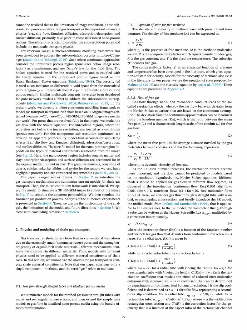
Fig. 1. 3D shale image reconstructed from FIB-SEM ( Ma et al., 2018 ). The size of the image is: 7.22 𝜇m ×5.11 𝜇m ×6.82 𝜇m; voxel size: 10 nm ×10 nm ×20 nm. Four material constituents are segmented: red - macro-pores; blue - organic mat- ter; pink - clay minerals; green - granular minerals. The shale sample is from a core in the Haynesville–Bossier shale formation.(For interpretation of the refer- ences to color in this figure legend, the reader is referred to the web version of this article.)

na

t

i

M

S

c

i

e

r

(

t

a

F

a

d

a

t

i

flS

K

a

s

f

fl

n

b

c

c

a

r

r

N

w

p

(

u

N

t

n

o

K

m

r

W

o

s

e

w

L

p

g

p

t

s

P

t

w

t

t

B

b

m

i

m

m

p

f

p

r

p

p

n

i

v

r

i

f

o

L

d

C

N

c

r

q

ano-CT, FIB-SEM, and HIM to characterize a shale sample of 1.3 3 cm

3

nd subsamples down to 3.25 3 𝜇m

3 . The highest resolution images ob-ained using HIM indicate that pores, which appeared to be isolatedn lower resolution FIB-SEM images, are connected by smaller pores.a et al. (2016) and Ma et al. (2018) used micro-CT, nano-CT, and FIB-

EM to address the issue of an REV for porosity and different materialonstituents. Their highest resolution FIB-SEM images were segmentednto four material constituents: macro-pores, organic matter, clay min-rals, and granular minerals. We note that pores are commonly catego-ized as micropores ( < 2 nm), mesopores (2–50 nm), and macropores > 50 nm) ( Rouquerol et al., 1994 ). Here, we use a different nomencla-ure and refer to the pores that are resolved in the image as macro-poresnd pores that are below the image resolution as sub-resolution pores.ig. 1 shows an example of a 3D FIB-SEM image from Ma et al. (2018) for shale sample from the Haynesville–Bossier shale formation. The 3Digital images show the complexity of the pore space of shale. The im-ge in Fig. 1 is used in our pore-scale simulation study (more details ofhe image are presented in Section 4 ).

The nanometer-range pores in shale rock lead to many interest-ng physical processes that deviate from the standard Darcy’s law forow in porous media, or the standard formulation of the Navier–tokes equations at the pore-scale. This dates back to the work oflinkenberg (1941) who reported that gas permeability of low perme-

71

ble tight rocks is larger than their intrinsic permeability (e.g., mea-ured with liquids), especially at low gas pressure. The Klinkenberg ef-ect can be attributed to a non-zero slip velocity at the pore wall. Gasow in small confined pores belongs to the subject of rarefied gas dy-amics. Small confined pores lead to gas rarefaction where collisionsetween pore wall and gas molecules become important relative to theollisions between gas molecules. The extent of the rarefaction effectan be characterized by the Knudsen number (Kn), which is defineds the ratio between the mean free path to the characteristic geomet-ic length of the flow conduit. Gas flow can be classified into fouregimes ( Karniadakis et al., 2005 ): continuum flow (Kn ≲ 0.001) whereavier–Stokes equations are applicable; slip flow (0.001 < Kn ≲ 0.1) inhich the Navier–Stokes equations can still be applied, but with ap-ropriate velocity slip conditions at the solid surface; transition flow0.1 < Kn ≲ 10) where gas flow transits from slip flow to free molec-lar flow; free molecular flow (Kn > 10) where the continuum-basedavier–Stokes equations are not applicable. Note that this classifica-

ion is based on gas flow through an infinite channel with the thick-ess being the characteristic length. The regime boundaries (in termsf Kn) depend on the specific geometries of the conduits. Beskok andarniadakis (1999) developed a unified model for rarefied gas flow inicro-channels, ducts, and pipes. Their model is applicable for all flow

egimes (0 ≤ Kn < ∞). We refer to the unified model as the BK model.u and Zhang (2016) extended the BK model to include the effects

f adsorption in the nano-channel accounting for migration of the ad-orbed phase. Civan (2010) used the BK model to develop an appar-nt permeability for tight rocks using the bundle-of-tubes model, whichas further extended to include surface diffusion ( Xiong et al., 2012 ).unati and Lee (2014) developed a bundle-of-dual-tubes model for gasroduction from fractured shale formations. In the spirit of the dusty-as model ( Mason and Malinauskas, 1983 ), another group of apparentermeability models has been derived by a linear, or weighted, summa-ion of the flux contributions from viscous flow, Knudsen diffusion, andurface diffusion (see Javadpour, 2009; Darabi et al., 2012; Sakhaee-our and Bryant, 2012; Wu et al., 2016 ). Landry et al. (2016) comparedhe BK model, the dusty-gas model, and the Javadpour (2009) modelith the linearized Boltzmann solution for a straight tube. They reported

hat both the dusty-gas and the Javadpour (2009) models overestimatehe permeability, while the BK model matches well with the linearizedoltzmann solution. In addition, Landry et al. (2016) showed that theundle-of-tubes model can significantly overestimate the apparent per-eability due to flow dependence on the pore shapes and connectivity

n the slip and early-transition flow regimes. To date, the apparent per-eability models in the literature are either limited to idealized porousedia (i.e., bundle-of-tubes with correction for tortuosity) or compositeorous media with a presumed distribution of constituents that allowor upscaling ( Darabi et al., 2012; Akkutlu et al., 2015 ). The appro-riate “apparent ” permeability and other transport properties of shaleocks remain open questions.

Images of shale samples provide an opportunity to model the com-lex transport dynamics directly for natural shale samples. This shouldrovide insight into the complex physics associated with transport inatural shales. The use of pore-scale imaging and numerical flow model-ng, referred to as digital rock physics or analysis, is increasing for reser-oir rocks ( Blunt et al., 2013; Blunt, 2017 ). For unconventional sourceocks (i.e., organic-rich shale), image-based pore-scale modeling is stilln its infancy. Lattice Boltzmann methods (LBM), as a popular methodor pore-scale simulation, has been used for direct numerical simulationf shale gas transport ( Wang et al., 2016 ). Various studies have extendedBM to include the transport physics relevant to shale, e.g., Knudseniffusion, slip flow, adsorption/desorption and surface diffusion (e.g.,hen et al., 2015; Wang et al., 2017 ). Another approach is to solve theavier–Stokes equations in the pore structures using finite-volume dis-retization schemes. Because most of the pores are in the nanometerange, the applicability of the standard Navier–Stokes equations may beuestioned. In addition, many pores with sizes in the nanometer range

B. Guo et al. Advances in Water Resources 122 (2018) 70–84

c

r

p

s

r

i

b

a

c

l

S

t

D

i

p

p

f

o

p

m

t

o

g

p

(

d

e

a

p

(

c

t

q

n

g

t

p

i

t

i

y

c

2

d

e

i

p

r

p

s

2

r

m

t

2

p

𝜌

w

w

R

“

a

t

i

M

e

2

c

t

t

u

f

g

K

w

m

𝜆

w

m

o

m

d

0

K

d

t

b

a

a

𝑞

w

a

l

𝑓

w

𝑓

w

a

e

c

b

fi

o

r

r

o

annot be resolved due to the limitation of image resolution. These sub-esolution pores are critical for gas transport as the important nanoscalehysics (e.g., slip flow, Knudsen diffusion, adsorption/desorption, andurface diffusion) primarily take place in those unresolved nano-porousegions. Therefore, it is crucial to consider the sub-resolution pores andnclude the nanoscale transport physics.

For reservoir rocks, a micro-continuum modeling framework haseen developed to address the sub-resolution porosity in micro-CT im-ges ( Soulaine and Tchelepi, 2016 ). Such micro-continuum approachesonsider the unresolved porous region (pore sizes below image reso-ution) as a continuum, and use Darcy’s law for the fluid flow. Thetokes equation is used for the resolved pores and is coupled withhe Darcy equation in the unresolved porous region based on thearcy–Brinkman–Stokes equations ( Brinkman, 1949 ). The porosity ( 𝜙)

s used as an indicator to differentiate void space from the unresolvedorous region ( 𝜙 = 1 represents void, 0 < 𝜙 < 1 represents sub-resolutionorous region). Similar multiscale concepts have also been developedor pore network models (PNM) to address the subresolution microp-rosity ( Mehmani and Prodanovi ć, 2014; Bultreys et al., 2015 ). In theresent work, we develop a micro-continuum modeling framework toodel gas transport in organic-rich shale based on 3D digital images (ob-

ained from micro-CT, nano-CT, or FIB-SEM; FIB-SEM images are used inur work). For pores that are resolved fully in the image, we model theas flow with the Stokes equation. The unresolved regions, where theore sizes are below the image resolution, are treated as a continuumporous medium). For this nanoporous sub-resolution continuum, weevelop an apparent permeability model that accounts for non-Darcyffects (i.e., slip flow and Knudsen diffusion), adsorption/desorption,nd surface diffusion. The specific model for the nano-porous region de-ends on the types of material constituents segmented from the imagesee Fig. 1 ). Here, the nano-porous region includes organic matter andlay; adsorption/desorption and surface diffusion are accounted for inhe organic matter, but not in clay. The granular minerals, consisting ofuartz, calcite, ankerite, albite, and pyrite for the sample we use, haveegligible porosity and are considered impermeable ( Ma et al., 2018 ).

The paper is organized as follows. In Section 2 we introduce theas transport mechanisms and summarize current models for shale gasransport. Then, the micro-continuum framework is introduced. We ap-ly the model to simulate a 3D FIB-SEM image (a subset of the imagen Fig. 1 ) to compute the apparent permeability. We then simulate theransient gas production process. Analysis of the numerical experimentss presented in Section 4 . Then, we discuss the implications of the anal-sis, the limitations of the model, and future directions in Section 5 . Welose with concluding remarks in Section 6 .

. Physics and modeling of shale gas transport

Gas transport in shale differs from that in conventional formationsue to the extremely small (nanometer range) pores and the strong het-rogeneity of organic-rich shale materials. Different mechanisms dom-nate the transport in different materials. Thus, models with differenthysics need to be applied to different material constituents of shaleock. In this section, we summarize the models for gas transport in com-lex shale material constituents. Note that our paper considers only aingle-component - methane, and the term “gas ” refers to methane.

.1. Gas flow through straight tubes and idealized porous media

We summarize models for the rarefied gas flow in straight tubes withadial and rectangular cross-sections, and then extend the simple tubeodels to gas flow in idealized nano-porous media using the bundle-of-

ubes representation.

72

.1.1. Equation-of-state for free methane

The density and viscosity of methane vary with pressure and tem-erature. The density of free methane ( 𝜌f ) can be expressed as

𝑓 =

𝑝 𝑓 𝑀

𝑍𝑅𝑇 , (1)

here p f is the pressure of free methane, M is the methane moleculareight, Z is the compressibility factor which equals to unity for ideal gas, is the gas constant, and T is the absolute temperature. The subscriptf ” denotes free gas.

The compressibility factor, Z , as an empirical function of pressurend temperature has been developed in the literature, which gives equa-ions of state for density. Models for the viscosity of methane also existn the literature. In our paper, we use the equation of state proposed byahmoud (2014) and the viscosity equation by Lee et al. (1966) . These

quations are presented in Appendix A .

.1.2. Flow of free gas

Gas flow through nano- and micro-scale conduits leads to the so-alled rarefaction effects, whereby the gas flow behavior deviates fromhe Navier–Stokes equations that are based on the continuum assump-ion. The deviation from the continuum approximation can be measuredsing the Knudsen number (Kn), which is the ratio between the meanree path ( 𝜆) and a characteristic length scale of the conduit ( L ) for freeas flow,

n =

𝜆

𝐿

, (2)

here the mean free path 𝜆 is the average distance traveled by the gasolecules between collisions and has the following expression

=

𝜇𝑓

𝑝 𝑓

√

𝜋𝑍𝑅𝑇

2 𝑀

, (3)

here 𝜇f is dynamic viscosity of free gas. As the Knudsen number increases, the rarefaction effects become

ore important, and the flow cannot be predicted by models basedn the continuum hypothesis, i.e., Navier–Stokes equations. Differentodels should be applied for gas flow in different flow regimes, asiscussed in the introduction (continuum flow: Kn ≲ 0.001, slip flow:.001 < Kn ≲ 0.1, transition flow: 0.1 < Kn ≲ 10, free molecular flow:n > 10). Here, we consider gas flow through a straight tube with a ra-ial, or rectangular, cross-section, and briefly introduce the BK model,he unified model from Beskok and Karniadakis (1999) , that is applica-le to all flow regimes. In the BK model, the volumetric flux q f through tube can be written as the Hagen–Poiseuille flux 𝑞 H−P ,𝑓 multiplied by correction factor, namely,

𝑓 = 𝑓 ( Kn ) 𝑞 H−P ,𝑓 , (4)

here the correction factor f (Kn) is a function of the Knudsen numbernd corrects for gas flow that deviates from continuum flow when Kn isarge. For a radial tube, f (Kn) is given by

( Kn ) = (1 + 𝛼Kn ) (1 +

4 Kn 1 − 𝑏 Kn

), (5)

hile for a rectangular tube, the correction factor is

( Kn ) = (1 + 𝛼Kn ) (1 +

6 Kn 1 − 𝑏 Kn

), (6)

here Kn = 𝜆∕ 𝑟 for a radial tube with r being the radius; Kn = 𝜆∕ ℎ for rectangular tube with h being the height; 𝐶 𝑟 ( Kn ) = 1 + 𝛼Kn is the rar-faction coefficient that models the effect of reduced inter-molecularollisions with increased Kn; 𝛼 is an coefficient that can be determinedy experiments or from linearized Boltzmann solution; b is the slip coef-cient and is determined as 𝑏 = −1 for tube flow representing a second-rder slip condition. For a radial tube, 𝑞 H−P ,𝑓 = 𝜋𝑟 4 ∕8∕ 𝜇𝑓 , while for a

ectangular tube, 𝑞 H−P ,𝑓 = 𝐶( AR ) 𝑤ℎ 3 ∕12∕ 𝜇𝑓 where w is the width of theectangular cross-section and C (AR) is the correction factor for the ge-metry that is a function of the aspect ratio of the rectangular channel

B. Guo et al. Advances in Water Resources 122 (2018) 70–84

(

a

t

fi

t

a

b

m

t

s

r

r

a

t

a

b

𝑘

w

p

a

(

𝑘

w

w

a

a

L

c

m

2

p

a

s

1

t

a

f

e

s

2

m

i

o

d

t

t

d

t

a

v

t

r

c

p

i

o

m

j

s

s

c

2

p

S

s

M

f

m

m

𝑓

w

𝛽

m

p

𝐮

i

a

m

a

o

i

e

a

(

L

𝑛

w

m

c

s

S

p

Č

d

𝐮

w

t

d

AR = 𝑤 ∕ ℎ ) and is independent of Kn. Note that f (Kn) →1 as Kn →0,nd q f recovers the Hagen–Poiseuille flux.

By comparing the volumetric flux predicted by Eqs. (5) and (6) withhe linearized Boltzmann solution, 𝛼 is fitted as an empirical analyticalunction 𝛼 = 𝛼0 (2∕ 𝜋) tan −1 ( 𝛼1 Kn 𝛽 ) with two free parameters 𝛼1 and 𝛽. 𝛼0 s determined by equating the flux predicted from Eqs. (5) and (6) tohe free molecular rate (Knudsen diffusion) when Kn →∞.

The BK model works well for rarefied gas flow in straight tubes forll flow regimes (0 ≤ Kn < ∞); however, a similar unified model has noteen developed for complex natural porous media, which consist ofany connected nano-scale pores and pore throats. Rarefied gas flow

hrough porous medium with low permeability (tight rocks) was firstystematically studied by Klinkenberg (1941) . Klinkenberg (1941) de-ived a model for gas flow through a straight capillary tube with a cor-ection of the slip boundary condition. He then introduced the so-calledpparent gas permeability for flow through an idealized porous mediumhat consists of a bundle of capillary tubes with the same diameter. Thepparent permeability can be written as a correction factor multipliedy the intrinsic permeability, k , as follows:

𝑎 =

(

1 +

𝑑

��

)

𝑘, (7)

here d is a constant and �� is the reciprocal mean gas pressure. Civan (2010) used the BK tube model and derived a unified apparent

ermeability model for an idealized porous medium blue consisting of bundle of tubes. Such model has a similar form as Eq. (7) by replacing1 + 𝑑∕ 𝑝 ) with f (Kn)

𝑎 = 𝑓 ( Kn ) 𝑘, (8)

here again k is the intrinsic permeability of the porous medium, whichas given by the Kozeny–Carman model in Civan (2010) .

We note that the bundle-of-nano-tubes model from Civan (2010) is simplified apparent permeability model for a nano-porous mediumnd can overestimate the apparent permeability as reported byandry et al. (2016) . More sophisticated models may be developed byonsidering the complex pore structures observed in natural shale for-ations.

.1.3. Adsorption/desorption and surface diffusion of adsorbed gas

The nano-tubes, or nano-porous materials, lead to extremely smallores and thus large surface areas on which gas can be adsorbed. Thedsorbed gas may also migrate along the pore wall, which is often con-idered as a diffusion process that is named surface diffusion ( Ruthven,984; Medve ď and Čern ỳ, 2011 ). The amount of adsorption depends onhe pressure and temperature of the free gas, and is often modeled byn isotherm that relates the amount of adsorption to the pressure of theree gas at a constant temperature. We discuss the details of the mod-ls for adsorbed gas in the following section when we consider specifichale material constituents.

.2. Gas transport in shale

Digital images of shale show strong heterogeneity of the differentaterial constituents (e.g., Fig. 1 ). In this section, based on the FIB-SEM

mages in Fig. 1 , we consider four material constituents: macro-pores,rganic matter, clay minerals, and granular minerals, and we employifferent models for each of them. Organic matter and clay both con-ain very small unresolved pores that are below the image resolution. Inhese sub-resolution pores, non-Darcy effects (i.e., slip flow and Knudseniffusion), adsorption/desorption, and surface diffusion can play impor-ant roles. We consider these unresolved regions as nano-porous materi-ls with connected sub-resolution pores and pore throats, and model thearious gas transport mechanisms at the continuum scale. Here, we usehe simple bundle-of-nano-tubes model for the unresolved nano-porousegions. The granular minerals have negligible porosity, allowing us toonsider them as impermeable materials, i.e., zero porosity and zero

73

ermeability. The macro-pores are pores that are fully resolved in themage; these macro-pores may belong to organic matter, clay minerals,r granular minerals. They can also bridge these three constituents. Weodel gas transport in macro-pores using the Stokes equation. This is

ustified based on the assumption that the macro-pores have large sizesuch that that the flow is either in the continuum flow regime, or thelip flow regime, where the Navier–Stokes equations (with velocity sliponditions) are applicable.

.2.1. Gas transport in organic matter

We consider the organic matter with sub-resolution pores as a nano-orous medium, and derive an apparent permeability model based onection 2.1 . In addition, we consider gas adsorption and surface diffu-ion.

odel for the apparent permeability

The organic matter has mostly circular pores and pore throats (seeor example the HIM images in Wu et al., 2017 ). For the apparent per-eability, we use the correction function from the bundle-of-nano-tubesodel derived from the BK model for radial tubes. Thus, we have

( Kn ) = (1 + 𝛼om Kn ) (1 +

4 Kn 1 + Kn

), (9)

here 𝛼om = 𝑎 0 , om 2 𝜋tan −1

(𝛼1 , om Kn βom

)with 𝑎 0 , om =

64 15 𝜋 , 𝛼1 , om = 4 . 0 ,

om = 0 . 4 . The subscript “om ” denotes organic matter. Then, using the correction function, flow of free gas in the organic

atter can be described by the Darcy-type equation with an apparentermeability k a , om

as

𝑓 = −

𝑘 𝑎, om

𝜇𝑓

∇ 𝑝 𝑓 = −

(1 + 𝛼om Kn ) (1 +

4 Kn 1+ Kn

)𝑘 om

𝜇𝑓

∇ 𝑝 𝑓 . (10)

Since the sub-resolution pores in the organic matter are not resolvedn the image, we need to make approximations for the porosity, perme-bility, and the average pore radius. Some of the information can be esti-ated from higher resolution TEM, or HIM, images of the organic matter

nd the pore size distribution measured from nitrogen adsorption. Webtain the Kn number based on the average radius and compute thentrinsic permeability k om

using the Kozeny–Carman model using thestimated porosity.

Experiments have shown that the Langmuir isotherm fits methanedsorption in organic-rich shale and isolated kerogen reasonably well Heller and Zoback, 2014; Rexer et al., 2014 ). As a result, we use theangmuir isotherm to model methane adsorption in the organic matter.

ad = 𝑛 max ad

𝐾𝑝 𝑓

1 + 𝐾𝑝 𝑓 , (11)

here n ad is the amount of adsorbed gas (mass per unit volume of porousaterial), 𝑛 max

ad is the maximum adsorption, K is the Langmuir coeffi-ient, which is the inverse of the pressure at which half of the adsorptionites are occupied.

urface diffusion

The adsorbed methane can migrate along the pore wall through arocess referred to as surface diffusion ( Ruthven, 1984; Medve ď andern ỳ, 2011 ). The volumetric flux of the adsorbed gas in organic matterue to surface diffusion can be written as

ad = −

1 𝜌ad

𝐷 𝑠 ∇ 𝑛 ad = −

1 𝜌ad

𝐷 𝑠 ∇

(

𝑛 max ad

𝐾𝑝 𝑓

1 + 𝐾𝑝 𝑓

)

, (12)

here u ad is the volumetric flow rate per unit area, 𝜌ad is the density ofhe adsorbed gas, D s is the surface diffusivity. Note that we assume theiffusion is isotropic and thus D is a scalar.

s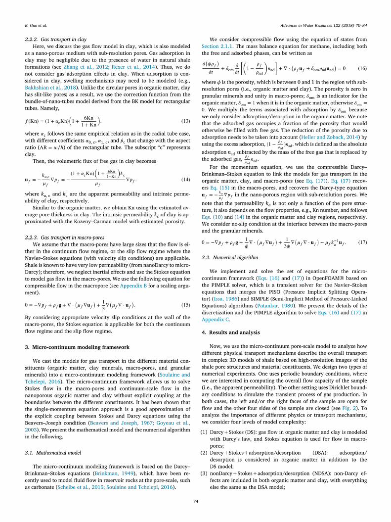

B. Guo et al. Advances in Water Resources 122 (2018) 70–84

2

a

c

f

n

s

B

h

b

t

𝑓

w

w

r

c

𝐮

w

a

e

p

2

t

N

S

D

t

c

m

0

B

m

fl

3

s

m

T

S

n

b

t

t

B

2

i

3

B

c

a

S

t

w

r

g

o

0

w

t

o

a

u

a

t

B

o

e

𝐮

n

t

E

W

a

0

3

c

t

e

t

E

d

A

4

d

i

s

n

w

(

a

b

fl

a

w

(

(

(

.2.2. Gas transport in clay

Here, we discuss the gas flow model in clay, which is also modeleds a nano-porous medium with sub-resolution pores. Gas adsorption inlay may be negligible due to the presence of water in natural shaleormations (see Zhang et al., 2012; Rexer et al., 2014 ). Thus, we doot consider gas adsorption effects in clay. When adsorption is con-idered in clay, swelling mechanisms may need to be modeled (e.g.,akhshian et al., 2018 ). Unlike the circular pores in organic matter, clayas slit-like pores; as a result, we use the correction function from theundle-of-nano-tubes model derived from the BK model for rectangularubes. Namely,

( Kn ) = (1 + 𝛼c Kn ) (1 +

6 Kn 1 + Kn

). (13)

here 𝛼c follows the same empirical relation as in the radial tube case,ith different coefficients 𝛼0, c , 𝛼1, c , and 𝛽c that change with the aspect

atio ( AR = 𝑤 ∕ ℎ ) of the rectangular tube. The subscript “c ” representslay.

Then, the volumetric flux of free gas in clay becomes

𝑓 = −

𝑘 𝑎, c

𝜇𝑓

∇ 𝑝 𝑓 = −

(1 + 𝛼c Kn ) (1 +

6 Kn 1+ Kn

)𝑘 c

𝜇𝑓

∇ 𝑝 𝑓 . (14)

here k a , c and k c are the apparent permeability and intrinsic perme-bility of clay, respectively.

Similar to the organic matter, we obtain Kn using the estimated av-rage pore thickness in clay. The intrinsic permeability k c of clay is ap-roximated with the Kozeny–Carman model with estimated porosity.

.2.3. Gas transport in macro-pores

We assume that the macro-pores have large sizes that the flow is ei-her in the continuum flow regime, or the slip flow regime where theavier–Stokes equations (with velocity slip conditions) are applicable.hale is known to have very low permeability (from nanoDarcy to micro-arcy); therefore, we neglect inertial effects and use the Stokes equation

o model gas flow in the macro-pores. We use the following equation forompressible flow in the macropore (see Appendix B for a scaling argu-ent).

= −∇ 𝑝 𝑓 + 𝜌𝑓 𝐠 + ∇ ⋅(𝜇𝑓 ∇ 𝐮 𝑓

)+

1 3 ∇

(𝜇𝑓 ∇ ⋅ 𝐮 𝑓

). (15)

y considering appropriate velocity slip conditions at the wall of theacro-pores, the Stokes equation is applicable for both the continuumow regime and the slip flow regime.

. Micro-continuum modeling framework

We cast the models for gas transport in the different material con-tituents (organic matter, clay minerals, macro-pores, and granularinerals) into a micro-continuum modeling framework ( Soulaine andchelepi, 2016 ). The micro-continuum framework allows us to solvetokes flow in the macro-pores and continuum-scale flow in theanoporous organic matter and clay without explicit coupling at theoundaries between the different constituents. It has been shown thathe single-momentum equation approach is a good approximation ofhe explicit coupling between Stokes and Darcy equations using theeavers–Joseph condition ( Beavers and Joseph, 1967; Goyeau et al.,003 ). We present the mathematical model and the numerical algorithmn the following.

.1. Mathematical model

The micro-continuum modeling framework is based on the Darcy–rinkman–Stokes equations ( Brinkman, 1949 ), which have been re-ently used to model fluid flow in reservoir rocks at the pore-scale, suchs carbonate ( Scheibe et al., 2015; Soulaine and Tchelepi, 2016 ).

74

We consider compressible flow using the equation of states fromection 2.1.1 . The mass balance equation for methane, including bothhe free and adsorbed phases, can be written as

𝜕 (𝜙𝜌𝑓

)𝜕𝑡

+ 𝛿om

𝜕

𝜕𝑡

[ (

1 −

𝜌𝑓

𝜌ad

)

𝑛 ad

] + ∇ ⋅

(𝜌𝑓 𝐮 𝑓 + 𝛿om

𝜌ad 𝐮 ad )= 0 (16)

here 𝜙 is the porosity, which is between 0 and 1 in the region with sub-esolution pores (i.e., organic matter and clay). The porosity is zero inranular minerals and unity in macro-pores; 𝛿om

is an indicator for therganic matter, 𝛿om = 1 when it is in the organic matter, otherwise 𝛿om = . We multiply the terms associated with adsorption by 𝛿om

becausee only consider adsorption/desorption in the organic matter. We note

hat the adsorbed gas occupies a fraction of the porosity that wouldtherwise be filled with free gas. The reduction of the porosity due todsorption needs to be taken into account ( Heller and Zoback, 2014 ) bysing the excess adsorption, (1 −

𝜌𝑓

𝜌ad ) 𝑛 ad , which is defined as the absolute

dsorption n ad subtracted by the mass of the free gas that is replaced byhe adsorbed gas,

𝜌𝑓

𝜌ad 𝑛 ad .

For the momentum equation, we use the compressible Darcy–rinkman–Stokes equation to link the models for gas transport in therganic matter, clay, and macro-pores (see Eq. (17) ). Eq. (17) recov-rs Eq. (15) in the macro-pores, and recovers the Darcy-type equation 𝑓 = −

𝑘 𝑎 𝜇𝑓

𝛻𝑝 𝑓 in the nano-porous region with sub-resolution pores. We

ote that the permeability k a is not only a function of the pore struc-ure, it also depends on the flow properties, e.g., Kn number, and followsqs. (10) and (14) in the organic matter and clay regions, respectively.e consider no-slip condition at the interface between the macro-pores

nd the granular minerals.

= −∇ 𝑝 𝑓 + 𝜌𝑓 𝐠 +

1 𝜙∇ ⋅

(𝜇𝑓 ∇ 𝐮 𝑓

)+

1 3 𝜙

∇

(𝜇𝑓 ∇ ⋅ 𝐮 𝑓

)− 𝜇𝑓 𝑘

−1 a 𝐮 𝑓 . (17)

.2. Numerical algorithm

We implement and solve the set of equations for the micro-ontinuum framework ( Eqs. (16) and (17) ) in OpenFOAM® based onhe PIMPLE solver, which is a transient solver for the Navier–Stokesquations that merges the PISO (Pressure Implicit Splitting Opera-or) ( Issa, 1986 ) and SIMPLE (Semi-Implicit Method of Pressure-Linkedquations) algorithms ( Patankar, 1980 ). We present the details of theiscretization and the PIMPLE algorithm to solve Eqs. (16) and (17) inppendix C .

. Results and analysis

Now, we use the micro-continuum pore-scale model to analyze howifferent physical transport mechanisms describe the overall transportn complex 3D models of shale based on high-resolution images of thehale pore structures and material constituents. We design two types ofumerical experiments. One uses periodic boundary conditions, wheree are interested in computing the overall flow capacity of the sample

i.e., the apparent permeability). The other setting uses Dirichlet bound-ry conditions to simulate the transient process of gas production. Inoth cases, the left and/or the right faces of the sample are open forow and the other four sides of the sample are closed (see Fig. 2 ). Tonalyze the importance of different physics or transport mechanisms,e consider four levels of model complexity:

1) Darcy+Stokes (DS): gas flow in organic matter and clay is modeledwith Darcy’s law, and Stokes equation is used for flow in macro-pores;

2) Darcy+Stokes+adsorption/desorption (DSA): adsorption/desorption is considered in organic matter in addition to theDS model;

3) nonDarcy+Stokes+adsorption/desorption (NDSA): non-Darcy ef-fects are included in both organic matter and clay, with everythingelse the same as the DSA model;

B. Guo et al. Advances in Water Resources 122 (2018) 70–84

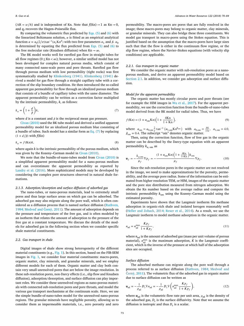
Fig. 2. Sketches of two numerical experiments for simulating gas transport on a 3D FIB-SEM image. In both scenarios, left and/or right boundaries are open for flow and the other four sizes are no-flow boundaries. The first scenario considers periodic boundary conditions to compute an apparent permeability, and the second scenario only allows the right boundary to be open at a fixed pressure ( 𝑝 𝑓 2 ) that is lower than the initial pressure in the sample ( 𝑝 𝑓 1 = 𝑝 𝑓 2 + Δ𝑝 ). The difference between the two pressures is small, Δ𝑝 ≪ 𝑝 𝑓 2 .

(

w

e

4

s

t

T

n

𝐿

(

m

c

m

r

s

a

U

f

fi

g

s

a

E

i

d

g

a

b

c

4

i

a

s

Fig. 3. A subsample of the full image in Fig. 1 . Size of the image: 3.56 𝜇m ×2.50 𝜇m ×3.36 𝜇m. (a) shows the overall image, and (b)–(e) show the distributions of the four material constituents: red - macro-pores, blue - organic matter, pink - clay minerals, green - granular minerals; (f) shows the two largest connected macro-pore networks.(For interpretation of the references to color in this figure legend, the reader is referred to the web version of this article.)

Table 1

Parameters used for the simulations. Note that or- ganic matter is assumed to have radial pores and the average pore size is the average pore radius; clay is assumed to have slit-like pores and the av- erage pore size refers to the average pore thick- ness.

Parameter Value

Porosity of organic matter ( 𝜙om ) 0.1 Porosity of clay ( 𝜙c ) 0.1 Average pore size in organic matter 5 nm

Average pore size in clay 5 nm

Langmuir coefficient ( K ) 4 ×10 −8 Pa −1

Maximum adsorption ( 𝑛 max ad ) 44.8 kg/m

3

Surface diffusion coefficient ( D s ) See Table 2 Density of adsorbed gas ( 𝜌ad ) 400 kg/m

3

Temperature 400 K

T

n

d

e

a

t

W

w

𝑝

4) nonDarcy+Stokes+adsorption/desorption+surface diffusion (fullmodel): this refers to the NDSA model with effects due to surfacediffusion of the adsorbed methane.

In the following subsections, we introduce the FIB-SEM images. Thene present the simulation results and analysis for the two numerical

xperiments and for all of the four models.

.1. FIB-SEM images used for the flow simulations

We use a subset of the original image shown in Fig. 1 for our pore-cale simulation. This is because using the original full image is compu-ationally expensive and becomes prohibitive for our detailed analysis.he sub-image is cut with each dimension being about half of the origi-al full image. The size of the sub-image is 𝐿 𝑥 = 3 . 56 𝜇m , 𝐿 𝑦 = 2 . 50 𝜇m ,

𝑧 = 3 . 36 𝜇m , and the voxel size is the same as the original full image Δ𝑥 = Δ𝑦 = 10 nm , Δ𝑧 = 20 nm ). Fig. 3 shows distributions of the fouraterial constituents in the sub-image. We also identify the two largest

onnected macro-pore clusters in Fig. 3 (f), which shows that there is aacro-pore network (the largest cluster) connecting the left face to the

ight face of the image. We will see later that this pore structure has aignificant impact on the results of the simulations. The 3D images werecquired in a Dual Beam FIB-SEM (Nova NanoLab 600i, FEI, Hillsboro,nited States) and they were aligned and sheared as a series of block

ace images before segmentation. A band-pass filter, non-local meanslter, sober filter and a top-hat filter were applied for the minerals, or-anic matter and pores segmentation. More details about the shale coreample, the acquisition procedures of the image, the image processingnd other measurements can be found in Ma et al. (2018)

We discretize the image with the finite-volume scheme and solveqs. (16) and (17) subject to the boundary conditions of the two numer-cal experiments. The numerical grid cells have a one-to-one correspon-ence with the digital voxels of the image, which leads to 14,952,000rid cells. Each voxel belongs to one of the four material constituents,nd is given a porosity. Voxels with 𝜙 = 1 belong to macro-pores, 𝜙 = 0elong to granular minerals, and 𝜙∈ (0, 1) represents organic matter andlay. 𝛿om = 1 when a voxel sits in organic matter, otherwise, 𝛿om = 0 .

.2. 3D simulations with periodic BCs: computing apparent permeability

In this section, we present the results and analysis of the first numer-cal experiment, which includes two parts. The first part computes andnalyzes the apparent permeability of organic matter and clay, and theecond part considers the apparent permeability of the 3D image.

75

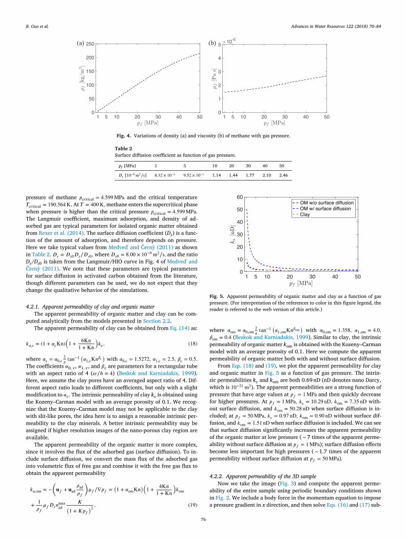
Here, we introduce the parameters we use for the simulation (seeable 1 ). The organic matter and the clay are assumed to be homoge-eous with a porosity of 0.1. The organic matter has an average pore ra-ius of 5 nm and the clay slit-pores have an average height of 5 nm. Thequation of state and the viscosity equation of methane give the densitynd viscosity range from 𝑝 = 1 MPa to 𝑝 = 50 MPa (see Fig. 4 ). Details ofhe equation of state and viscosity equation are shown in Appendix A .

e consider an isothermal system with a temperature of 400 K. Ase can see, density of methane changes drastically from 𝑝 = 1 MPa to = 50 MPa , while the viscosity has much less variation. The critical

B. Guo et al. Advances in Water Resources 122 (2018) 70–84

Fig. 4. Variations of density (a) and viscosity (b) of methane with gas pressure.

Table 2

Surface diffusion coefficient as function of gas pressure.

p f [MPa] 1 5 10 20 30 40 50

D s [ 10 −8 m 2 ∕s ] 8 . 32 × 10 −1 9 . 52 × 10 −1 1.14 1.44 1.77 2.10 2.46

p

𝑇

w

T

s

f

t

H

i

D

Č

f

t

c

4

p

𝑘

w

T

w

H

f

m

t

n

w

m

a

a

s

c

i

o

Fig. 5. Apparent permeability of organic matter and clay as a function of gas pressure. (For interpretation of the references to color in this figure legend, the reader is referred to the web version of this article.)

w

𝛽

p

m

p

a

s

w

p

f

o

c

f

t

o

a

b

p

4

a

i

a

ressure of methane 𝑝 critical = 4 . 599 MPa and the critical temperature critical = 190 . 564 K. At 𝑇 = 400 K, methane enters the supercritical phasehen pressure is higher than the critical pressure 𝑝 critical = 4 . 599 MPa .he Langmuir coefficient, maximum adsorption, and density of ad-orbed gas are typical parameters for isolated organic matter obtainedrom Rexer et al. (2014) . The surface diffusion coefficient ( D s ) is a func-ion of the amount of adsorption, and therefore depends on pressure.ere we take typical values from Medve ď and Čern ỳ (2011) as shown

n Table 2 . 𝐷 𝑠 = 𝐷 𝑠 0 𝐷 𝑠 ∕ 𝐷 𝑠 0 , where 𝐷 𝑠 0 = 8 . 00 × 10 −9 m

2 ∕s , and the ratio s / D s 0 is taken from the Langmuir/HIO curve in Fig. 4 of Medve ď andern ỳ (2011) . We note that these parameters are typical parameters

or surface diffusion in activated carbon obtained from the literature,hough different parameters can be used, we do not expect that theyhange the qualitative behavior of the simulations.

.2.1. Apparent permeability of clay and organic matter

The apparent permeability of organic matter and clay can be com-uted analytically from the models presented in Section 2.2 .

The apparent permeability of clay can be obtained from Eq. (14) as:

𝑎, c = (1 + 𝛼c Kn ) (1 +

6 Kn 1 + Kn

)𝑘 c , (18)

here 𝛼c = 𝛼0 , c 2 𝜋tan −1

(𝛼1 , c Kn 𝛽c

)with 𝛼0 , c = 1 . 5272 , 𝛼1 , c = 2 . 5 , 𝛽c = 0 . 5 .

he coefficients 𝛼0, c , 𝛼1, c , and 𝛽c are parameters for a rectangular tubeith an aspect ratio of 4 ( 𝑤 ∕ ℎ = 4 ) ( Beskok and Karniadakis, 1999 ).ere, we assume the clay pores have an averaged aspect ratio of 4. Dif-

erent aspect ratio leads to different coefficients, but only with a slightodification to 𝛼c . The intrinsic permeability of clay k c is obtained using

he Kozeny–Carman model with an average porosity of 0.1. We recog-ize that the Kozeny–Carman model may not be applicable to the clayith slit-like pores, the idea here is to assign a reasonable intrinsic per-eability to the clay minerals. A better intrinsic permeability may be

ssigned if higher resolution images of the nano-porous clay region arevailable.

The apparent permeability of the organic matter is more complex,ince it involves the flux of the adsorbed gas (surface diffusion). To in-lude surface diffusion, we convert the mass flux of the adsorbed gasnto volumetric flux of free gas and combine it with the free gas flux tobtain the apparent permeability

𝑘 𝑎, om = −

(

𝐮 𝑓 + 𝐮 ad 𝜌ad 𝜌𝑓

)

𝜇𝑓 ∕∇ 𝑝 𝑓 =

(1 + 𝛼om Kn

)(1 +

4 Kn 1 + Kn

)𝑘 om

+

1 𝜌𝑓

𝜇𝑓 𝐷 𝑠 𝑛 max ad

𝐾 (1 + 𝐾𝑝 𝑓

)2 , (19)

76

here 𝛼om = 𝛼0 , om 2 𝜋tan −1

(𝛼1 , om Kn 𝛽om

)with 𝛼0 , om = 1 . 358 , 𝛼1 , om = 4 . 0 ,

om = 0 . 4 ( Beskok and Karniadakis, 1999 ). Similar to clay, the intrinsicermeability of organic matter k om

is obtained with the Kozeny–Carmanodel with an average porosity of 0.1. Here we compute the apparentermeability of organic matter both with and without surface diffusion.

From Eqs. (18) and (19) , we plot the apparent permeability for claynd organic matter in Fig. 5 as a function of gas pressure. The intrin-ic permeabilities k c and k om

are both 0.69 nD (nD denotes nano Darcy,hich is 10 −21 m

2 ). The apparent permeabilities are a strong function ofressure that have arge values at 𝑝 𝑓 = 1 MPa and then quickly decreaseor higher pressures. At 𝑝 𝑓 = 1 MPa , 𝑘 c = 10 . 29 nD , 𝑘 om = 7 . 35 nD with-ut surface diffusion, and 𝑘 om = 50 . 28 nD when surface diffusion is in-luded; at 𝑝 𝑓 = 50 MPa , 𝑘 c = 0 . 97 nD , 𝑘 om = 0 . 90 nD without surface dif-usion, and 𝑘 om = 1 . 51 nD when surface diffusion is included. We can seehat surface diffusion significantly increases the apparent permeabilityf the organic matter at low pressure ( ∼7 times of the apparent perme-bility without surface diffusion at 𝑝 𝑓 = 1 MPa ); surface diffusion effectsecome less important for high pressures ( ∼1.7 times of the apparentermeability without surface diffusion at 𝑝 𝑓 = 50 MPa ).

.2.2. Apparent permeability of the 3D sample

Now we take the image ( Fig. 3 ) and compute the apparent perme-bility of the entire sample using periodic boundary conditions shownn Fig. 2 . We include a body force in the momentum equation to impose pressure gradient in x direction, and then solve Eqs. (16) and (17) sub-

B. Guo et al. Advances in Water Resources 122 (2018) 70–84

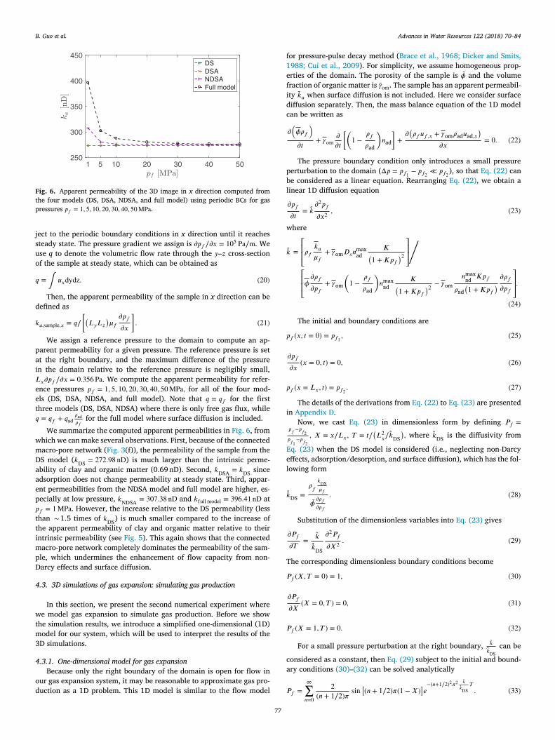
Fig. 6. Apparent permeability of the 3D image in x direction computed from

the four models (DS, DSA, NDSA, and full model) using periodic BCs for gas pressures 𝑝 𝑓 = 1 , 5 , 10 , 20 , 30 , 40 , 50 MPa .

j

s

u

o

𝑞

d

𝑘

p

a

i

𝐿

e

e

t

𝑞

w

m

D

a

a

e

p

𝑝

t

t

i

m

p

D

4

w

t

m

3

4

o

d

f

1

e

f

i

d

c

p

b

l

w

𝑘

𝑝

𝑝

i

E

e

l

𝑘

T

𝑃

𝑃

c

a

𝑃

ect to the periodic boundary conditions in x direction until it reachesteady state. The pressure gradient we assign is ∂ 𝑝 𝑓 ∕∂ 𝑥 = 10 5 Pa∕m . Wese q to denote the volumetric flow rate through the 𝑦 –𝑧 cross-sectionf the sample at steady state, which can be obtained as

= ∫ 𝑢 𝑥 dy dz . (20)

Then, the apparent permeability of the sample in x direction can beefined as

𝑎, sample ,𝑥 = 𝑞 ∕ [ (

𝐿 𝑦 𝐿 𝑧

)𝜇𝑓

𝜕 𝑝 𝑓

𝜕 𝑥

] . (21)

We assign a reference pressure to the domain to compute an ap-arent permeability for a given pressure. The reference pressure is sett the right boundary, and the maximum difference of the pressuren the domain relative to the reference pressure is negligibly small, 𝑥 𝜕 𝑝 𝑓 ∕ 𝜕 𝑥 = 0 . 356 Pa . We compute the apparent permeability for refer-nce pressures 𝑝 𝑓 = 1 , 5 , 10 , 20 , 30 , 40 , 50 MPa , for all of the four mod-ls (DS, DSA, NDSA, and full model). Note that 𝑞 = 𝑞 𝑓 for the firsthree models (DS, DSA, NDSA) where there is only free gas flux, while = 𝑞 𝑓 + 𝑞 ad

𝜌ad 𝜌𝑓

for the full model where surface diffusion is included.

We summarize the computed apparent permeabilities in Fig. 6 , fromhich we can make several observations. First, because of the connectedacro-pore network ( Fig. 3 (f)), the permeability of the sample from theS model ( 𝑘 DS = 272 . 98 nD ) is much larger than the intrinsic perme-bility of clay and organic matter (0.69 nD). Second, 𝑘 DSA = 𝑘 DS sincedsorption does not change permeability at steady state. Third, appar-nt permeabilities from the NDSA model and full model are higher, es-ecially at low pressure, 𝑘 NDSA = 307 . 38 nD and 𝑘 full model = 396 . 41 nD at 𝑓 = 1 MPa . However, the increase relative to the DS permeability (lesshan ∼1.5 times of 𝑘 DS ) is much smaller compared to the increase ofhe apparent permeability of clay and organic matter relative to theirntrinsic permeability (see Fig. 5 ). This again shows that the connectedacro-pore network completely dominates the permeability of the sam-le, which undermines the enhancement of flow capacity from non-arcy effects and surface diffusion.

.3. 3D simulations of gas expansion: simulating gas production

In this section, we present the second numerical experiment wheree model gas expansion to simulate gas production. Before we show

he simulation results, we introduce a simplified one-dimensional (1D)odel for our system, which will be used to interpret the results of theD simulations.

.3.1. One-dimensional model for gas expansion

Because only the right boundary of the domain is open for flow inur gas expansion system, it may be reasonable to approximate gas pro-uction as a 1D problem. This 1D model is similar to the flow model

77

or pressure-pulse decay method ( Brace et al., 1968; Dicker and Smits,988; Cui et al., 2009 ). For simplicity, we assume homogeneous prop-rties of the domain. The porosity of the sample is �� and the volumeraction of organic matter is 𝛾om . The sample has an apparent permeabil-ty �� 𝑎 when surface diffusion is not included. Here we consider surfaceiffusion separately. Then, the mass balance equation of the 1D modelan be written as

𝜕 (𝜙𝜌𝑓

)𝜕𝑡

+ 𝛾om 𝜕

𝜕𝑡

[ (

1 −

𝜌𝑓

𝜌ad

)

𝑛 ad

] +

𝜕 (𝜌𝑓 𝑢 𝑓 ,𝑥 + 𝛾om

𝜌ad 𝑢 ad ,𝑥 )

𝜕𝑥 = 0 . (22)

The pressure boundary condition only introduces a small pressureerturbation to the domain ( Δ𝑝 = 𝑝 𝑓 1 − 𝑝 𝑓 2 ≪ 𝑝 𝑓 2 ), so that Eq. (22) cane considered as a linear equation. Rearranging Eq. (22) , we obtain ainear 1D diffusion equation

𝜕𝑝 𝑓

𝜕𝑡 = ��

𝜕 2 𝑝 𝑓

𝜕𝑥 2 , (23)

here

=

⎡ ⎢ ⎢ ⎣ 𝜌𝑓

𝑘 𝑎 𝜇𝑓

+ 𝛾om

𝐷 𝑠 𝑛 max ad

𝐾 (1 + 𝐾𝑝 𝑓

)2 ⎤ ⎥ ⎥ ⎦ /

⎡ ⎢ ⎢ ⎣ 𝜙𝜕𝜌𝑓

𝜕𝑝 𝑓 + 𝛾om

(

1 −

𝜌𝑓

𝜌ad

)

𝑛 max ad

𝐾 (1 + 𝐾𝑝 𝑓

)2 − 𝛾om

𝑛 max ad

𝐾𝑝 𝑓

𝜌ad (1 + 𝐾𝑝 𝑓

) 𝜕𝜌𝑓

𝜕𝑝 𝑓

⎤ ⎥ ⎥ ⎦ . (24)

The initial and boundary conditions are

𝑓 ( 𝑥, 𝑡 = 0) = 𝑝 𝑓 1 , (25)

𝜕𝑝 𝑓

𝜕𝑥 ( 𝑥 = 0 , 𝑡 ) = 0 , (26)

𝑓 ( 𝑥 = 𝐿 𝑥 , 𝑡 ) = 𝑝 𝑓 2 . (27)

The details of the derivations from Eq. (22) to Eq. (23) are presentedn Appendix D .

Now, we cast Eq. (23) in dimensionless form by defining 𝑃 𝑓 =𝑝 𝑓 − 𝑝

𝑓 2 𝑝 𝑓 1

− 𝑝 𝑓 2

, 𝑋 = 𝑥 ∕ 𝐿 𝑥 , 𝑇 = 𝑡 ∕ (𝐿

2 𝑥 ∕ 𝑘 DS

), where �� DS is the diffusivity from

q. (23) when the DS model is considered (i.e., neglecting non-Darcyffects, adsorption/desorption, and surface diffusion), which has the fol-owing form

DS =

𝜌𝑓

𝑘 DS 𝜇𝑓

��𝜕𝜌𝑓

𝜕𝑝 𝑓

. (28)

Substitution of the dimensionless variables into Eq. (23) gives

𝜕𝑃 𝑓

𝜕𝑇 =

��

�� DS

𝜕 2 𝑃 𝑓

𝜕𝑋

2 . (29)

he corresponding dimensionless boundary conditions become

𝑓 ( 𝑋, 𝑇 = 0 ) = 1 , (30)

𝜕𝑃 𝑓

𝜕𝑋

( 𝑋 = 0 , 𝑇 ) = 0 , (31)

𝑓 ( 𝑋 = 1 , 𝑇 ) = 0 . (32)

For a small pressure perturbation at the right boundary, ��

�� DS can be

onsidered as a constant, then Eq. (29) subject to the initial and bound-ry conditions (30) –(32) can be solved analytically

𝑓 =

∞∑𝑛 =0

2 ( 𝑛 + 1∕2 ) 𝜋

sin [( 𝑛 + 1∕2 ) 𝜋( 1 − 𝑋 )

]𝑒 − ( 𝑛 +1∕2 ) 2 𝜋2 ��

�� DS 𝑇

. (33)

B. Guo et al. Advances in Water Resources 122 (2018) 70–84

𝑃

t

n

t

t

a

𝑀

fl

𝑀

d

s

t

i

p

4

s

g

t

a

a

r

t

t

p

s

(

m

𝑝

i

(

p

n

i

t

e

t

r

b

b

t

f

c

I

w

D

s

n

p

p

d

s

f

t

g

r

f

s

h

i

c

p

t

t

m

s

w

A

f

a

p

c

t

o

4

d

o

m

t

g

t

t

d

r

f

r

F

o

i

a

r

f

s

p

a

d

c

s

d

d

(

s

d

p

c

d

t

Approximating P f using the first term of the series solution (33) gives

𝑓 =

4 𝜋sin

(1 2

𝜋( 1 − 𝑋 ) )𝑒 − 1 4 𝜋

2 ��

�� DS 𝑇

. (34)

From the pressure solution Eq. (34) , we can derive the expression forhe outlet mass flow rate (production rate) at the right boundary. We

ondimensionalize the outlet mass flow rate by �� DS = − 𝜌𝑓

𝑘 DS 𝜇𝑓

𝑝 𝑓 2 − 𝑝 𝑓 1 𝐿 𝑥

,

he characteristic outlet mass flow rate from the DS model, and obtainhe dimensionless outlet mass flow rate (not including surface diffusion)s

= �� ∕ 𝑚 DS = −

�� 𝑎 𝑘 DS

𝜕𝑃 𝑓

𝜕𝑋

|𝑋=1 = 2 �� 𝑎 𝑘 DS

𝑒 − 1 4 𝜋

2 ��

�� DS 𝑇

. (35)

When surface diffusion is included, the dimensionless outlet massow rate becomes

= �� ∕ 𝑚 𝑐

=

[𝜌𝑓 𝑢 𝑓 ,𝑥 + 𝜌ad 𝑢 ad ,𝑥

]|𝑋=1

�� 𝑐

= 2 ⎡ ⎢ ⎢ ⎣

�� 𝑎 𝑘 DS

+ 𝛾om 𝐷 𝑠 𝑛 max ad

𝐾𝜇𝑓

𝜌𝑓 𝑘 DS (1 + 𝐾𝑝 𝑓

)2 ⎤ ⎥ ⎥ ⎦ 𝑒 − 1 4 𝜋

2 ��

�� DS 𝑇 . (36)

Eqs. (35) and (36) show that the dimensionless outlet mass flow rateeclines exponentially with dimensionless time, T . ln �� ∼ 𝑇 with the

lope −

1 4 𝜋

2 ��

�� DS representing the flow capacity of the shale sample. In

he following section, we use the results and analysis of the 1D model tonterpret the production decline results from the 3D simulations of gasroduction.

.3.2. Production decline

We simulate gas production for 𝑝 𝑓 = 1 MPa and 𝑝 𝑓 = 50 MPa , repre-enting low and high pressures, respectively. Pressure p f refers to theas pressure at the right boundary 𝑝 𝑓 2 . The difference between the ini-ial pressure ( 𝑝 𝑓 1 ) in the domain and the boundary pressure ( 𝑝 𝑓 2 ) is kepts Δ𝑝 = 100 Pa ≪ 𝑝 𝑓 . Integrating the mass flux across the right bound-ry, we obtain the outlet mass flow rate. We normalize the mass flowate using the characteristic mass flow rate from the DS model, �� DS , in-roduced in Section 4.3.1 , and nondimensionalize the time scale usinghe characteristic time scale from the DS model, 𝑇 DS = 𝐿

2 𝑥 ∕ 𝑘 DS . Then, we

lot the dimensionless mass flow rate with the dimensionless time on aemi-log scale, for both early time (0 < T < 0.1) and late time (0 < T < 10)see Fig. 7 ).

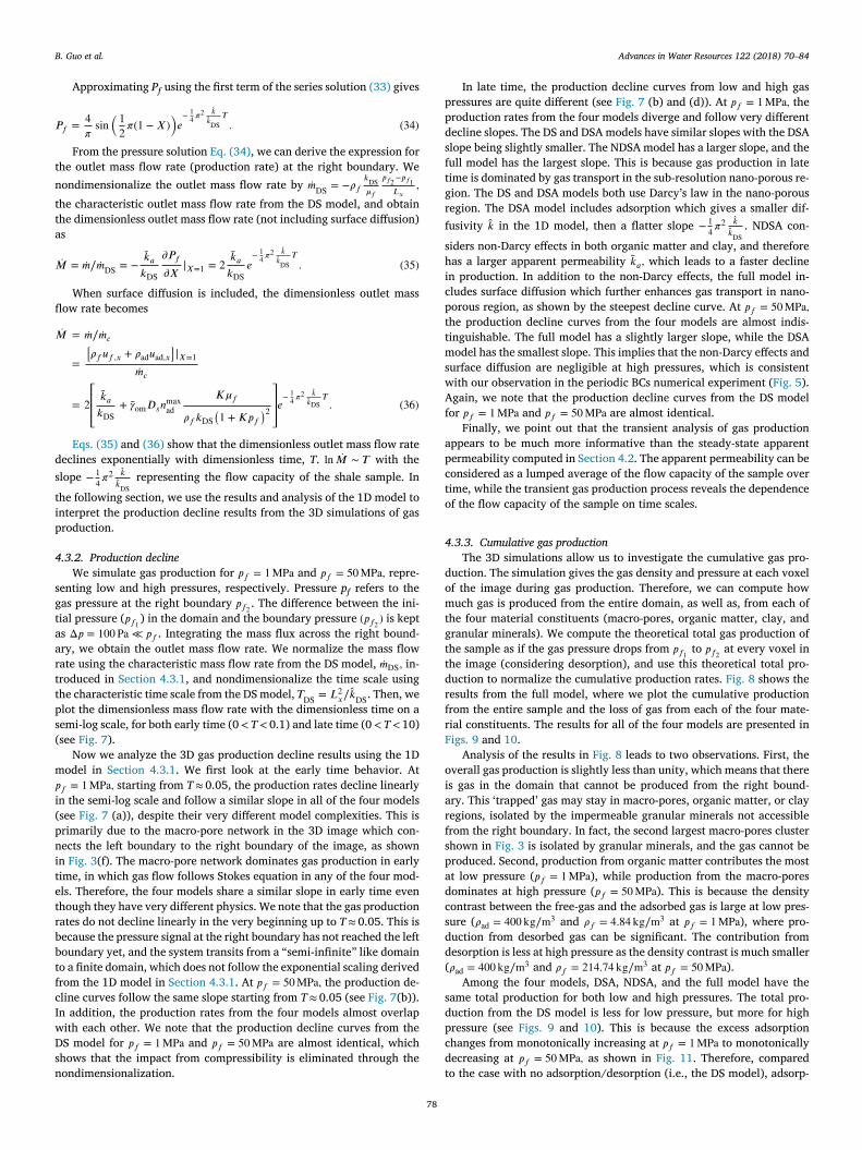
Now we analyze the 3D gas production decline results using the 1Dodel in Section 4.3.1 . We first look at the early time behavior. At 𝑓 = 1 MPa , starting from T ≈0.05, the production rates decline linearlyn the semi-log scale and follow a similar slope in all of the four modelssee Fig. 7 (a)), despite their very different model complexities. This isrimarily due to the macro-pore network in the 3D image which con-ects the left boundary to the right boundary of the image, as shownn Fig. 3 (f). The macro-pore network dominates gas production in earlyime, in which gas flow follows Stokes equation in any of the four mod-ls. Therefore, the four models share a similar slope in early time evenhough they have very different physics. We note that the gas productionates do not decline linearly in the very beginning up to T ≈0.05. This isecause the pressure signal at the right boundary has not reached the leftoundary yet, and the system transits from a “semi-infinite ” like domaino a finite domain, which does not follow the exponential scaling derivedrom the 1D model in Section 4.3.1 . At 𝑝 𝑓 = 50 MPa , the production de-line curves follow the same slope starting from T ≈0.05 (see Fig. 7 (b)).n addition, the production rates from the four models almost overlapith each other. We note that the production decline curves from theS model for 𝑝 𝑓 = 1 MPa and 𝑝 𝑓 = 50 MPa are almost identical, which

hows that the impact from compressibility is eliminated through theondimensionalization.

78

In late time, the production decline curves from low and high gasressures are quite different (see Fig. 7 (b) and (d)). At 𝑝 𝑓 = 1 MPa , theroduction rates from the four models diverge and follow very differentecline slopes. The DS and DSA models have similar slopes with the DSAlope being slightly smaller. The NDSA model has a larger slope, and theull model has the largest slope. This is because gas production in lateime is dominated by gas transport in the sub-resolution nano-porous re-ion. The DS and DSA models both use Darcy’s law in the nano-porousegion. The DSA model includes adsorption which gives a smaller dif-

usivity �� in the 1D model, then a flatter slope −

1 4 𝜋

2 ��

�� DS . NDSA con-

iders non-Darcy effects in both organic matter and clay, and thereforeas a larger apparent permeability �� 𝑎 , which leads to a faster declinen production. In addition to the non-Darcy effects, the full model in-ludes surface diffusion which further enhances gas transport in nano-orous region, as shown by the steepest decline curve. At 𝑝 𝑓 = 50 MPa ,he production decline curves from the four models are almost indis-inguishable. The full model has a slightly larger slope, while the DSAodel has the smallest slope. This implies that the non-Darcy effects and

urface diffusion are negligible at high pressures, which is consistentith our observation in the periodic BCs numerical experiment ( Fig. 5 ).gain, we note that the production decline curves from the DS model

or 𝑝 𝑓 = 1 MPa and 𝑝 𝑓 = 50 MPa are almost identical. Finally, we point out that the transient analysis of gas production

ppears to be much more informative than the steady-state apparentermeability computed in Section 4.2 . The apparent permeability can beonsidered as a lumped average of the flow capacity of the sample overime, while the transient gas production process reveals the dependencef the flow capacity of the sample on time scales.

.3.3. Cumulative gas production

The 3D simulations allow us to investigate the cumulative gas pro-uction. The simulation gives the gas density and pressure at each voxelf the image during gas production. Therefore, we can compute howuch gas is produced from the entire domain, as well as, from each of

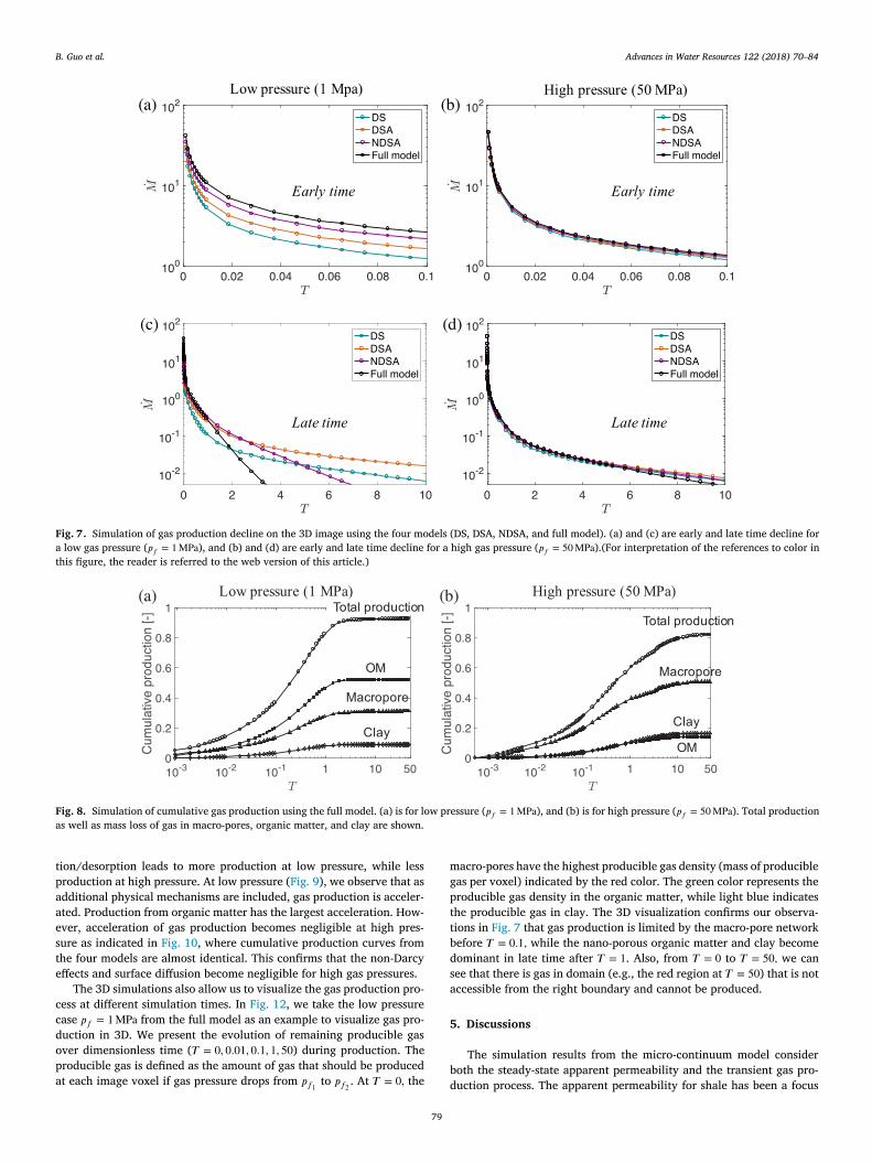
he four material constituents (macro-pores, organic matter, clay, andranular minerals). We compute the theoretical total gas production ofhe sample as if the gas pressure drops from 𝑝 𝑓 1 to 𝑝 𝑓 2 at every voxel inhe image (considering desorption), and use this theoretical total pro-uction to normalize the cumulative production rates. Fig. 8 shows theesults from the full model, where we plot the cumulative productionrom the entire sample and the loss of gas from each of the four mate-ial constituents. The results for all of the four models are presented inigs. 9 and 10 .

Analysis of the results in Fig. 8 leads to two observations. First, theverall gas production is slightly less than unity, which means that theres gas in the domain that cannot be produced from the right bound-ry. This ‘trapped’ gas may stay in macro-pores, organic matter, or clayegions, isolated by the impermeable granular minerals not accessiblerom the right boundary. In fact, the second largest macro-pores clusterhown in Fig. 3 is isolated by granular minerals, and the gas cannot beroduced. Second, production from organic matter contributes the mostt low pressure ( 𝑝 𝑓 = 1 MPa ), while production from the macro-poresominates at high pressure ( 𝑝 𝑓 = 50 MPa ). This is because the densityontrast between the free-gas and the adsorbed gas is large at low pres-ure ( 𝜌ad = 400 kg∕m

3 and 𝜌𝑓 = 4 . 84 kg∕m

3 at 𝑝 𝑓 = 1 MPa ), where pro-uction from desorbed gas can be significant. The contribution fromesorption is less at high pressure as the density contrast is much smaller 𝜌ad = 400 kg∕m

3 and 𝜌𝑓 = 214 . 74 kg∕m

3 at 𝑝 𝑓 = 50 MPa ). Among the four models, DSA, NDSA, and the full model have the

ame total production for both low and high pressures. The total pro-uction from the DS model is less for low pressure, but more for highressure (see Figs. 9 and 10 ). This is because the excess adsorptionhanges from monotonically increasing at 𝑝 𝑓 = 1 MPa to monotonicallyecreasing at 𝑝 𝑓 = 50 MPa , as shown in Fig. 11 . Therefore, comparedo the case with no adsorption/desorption (i.e., the DS model), adsorp-

B. Guo et al. Advances in Water Resources 122 (2018) 70–84

Fig. 7. Simulation of gas production decline on the 3D image using the four models (DS, DSA, NDSA, and full model). (a) and (c) are early and late time decline for a low gas pressure ( 𝑝 𝑓 = 1 MPa ), and (b) and (d) are early and late time decline for a high gas pressure ( 𝑝 𝑓 = 50 MPa ).(For interpretation of the references to color in this figure, the reader is referred to the web version of this article.)

Fig. 8. Simulation of cumulative gas production using the full model. (a) is for low pressure ( 𝑝 𝑓 = 1 MPa ), and (b) is for high pressure ( 𝑝 𝑓 = 50 MPa ). Total production as well as mass loss of gas in macro-pores, organic matter, and clay are shown.

t

p

a

a

e

s

t

e

c

c

d

o

p

a

m

g

p

t

t

b

d

s

a

5

b

d

ion/desorption leads to more production at low pressure, while lessroduction at high pressure. At low pressure ( Fig. 9 ), we observe that asdditional physical mechanisms are included, gas production is acceler-ted. Production from organic matter has the largest acceleration. How-ver, acceleration of gas production becomes negligible at high pres-ure as indicated in Fig. 10 , where cumulative production curves fromhe four models are almost identical. This confirms that the non-Darcyffects and surface diffusion become negligible for high gas pressures.

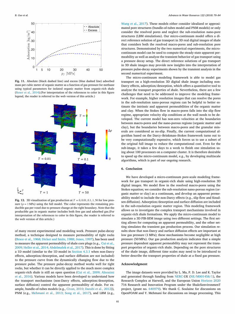
The 3D simulations also allow us to visualize the gas production pro-ess at different simulation times. In Fig. 12 , we take the low pressurease 𝑝 𝑓 = 1 MPa from the full model as an example to visualize gas pro-uction in 3D. We present the evolution of remaining producible gasver dimensionless time ( 𝑇 = 0 , 0 . 01 , 0 . 1 , 1 , 50 ) during production. Theroducible gas is defined as the amount of gas that should be producedt each image voxel if gas pressure drops from 𝑝 𝑓 1 to 𝑝 𝑓 2 . At 𝑇 = 0 , the

79

acro-pores have the highest producible gas density (mass of producibleas per voxel) indicated by the red color. The green color represents theroducible gas density in the organic matter, while light blue indicateshe producible gas in clay. The 3D visualization confirms our observa-ions in Fig. 7 that gas production is limited by the macro-pore networkefore 𝑇 = 0 . 1 , while the nano-porous organic matter and clay becomeominant in late time after 𝑇 = 1 . Also, from 𝑇 = 0 to 𝑇 = 50 , we canee that there is gas in domain (e.g., the red region at 𝑇 = 50 ) that is notccessible from the right boundary and cannot be produced.

. Discussions

The simulation results from the micro-continuum model consideroth the steady-state apparent permeability and the transient gas pro-uction process. The apparent permeability for shale has been a focus

B. Guo et al. Advances in Water Resources 122 (2018) 70–84

Fig. 9. Simulation of cumulative gas production at low pressure ( 𝑝 𝑓 = 1 MPa ) using the four models (DS, DSA, NDSA, and full model). (a) shows the total gas production, and (b)–(d) represent the mass loss in the sample from macro-pores, organic matter, and clay, over time. (For interpretation of the references to color in this figure legend, the reader is referred to the web version of this article.)

Fig. 10. Simulation of cumulative gas production at high pressure ( 𝑝 𝑓 = 50 MPa ) using the four models (DS, DSA, NDSA, and full model). (a) shows the total gas production, and (b)–(d) represent the mass loss in the sample from macro-pores, organic matter, and clay, over time. (For interpretation of the references to color in this figure legend, the reader is referred to the web version of this article.)

80

B. Guo et al. Advances in Water Resources 122 (2018) 70–84

Fig. 11. Absolute (black dashed line) and excess (blue dashed line) adsorbed mass per cubic meter of organic matter as a function of gas pressure for methane using typical parameters for isolated organic matter from organic-rich shale ( Rexer et al., 2014 ).(For interpretation of the references to color in this figure legend, the reader is referred to the web version of this article.)

Fig. 12. 3D visualization of gas production at 𝑇 = 0 , 0 . 01 , 0 . 1 , 1 , 50 for low pres- sure ( 𝑝 = 1 MPa ) using the full model. The color represents the remaining pro- ducible gas per voxel due to pressure change at the right boundary. Note that the producible gas in organic matter includes both free gas and adsorbed gas.(For interpretation of the references to color in this figure, the reader is referred to the web version of this article.)

o

m

(

t

2

a

e

t

p

r

o

e

t

s

a

P

W

m

c

s

r

t

s

c

m

a

i

p

s

t

D

a

c

w

i

t

a

r

v

b

c

e

g

b

t

s

i

t

a

6

w

d

S

g

a

s

i

a

o

s

t

t

s

l

p

p

p

o

b

A

a

R

7

p

O

f many recent experimental and modeling work. Pressure pulse-decayethod, a technique designed to measure permeability of tight rocks

Brace et al., 1968; Dicker and Smits, 1988; Jones, 1997 ), has been usedo measure the apparent permeability of shale core plugs (e.g., Cui et al.,009; Heller et al., 2014; Abdelmalek et al., 2017 ). This is done by fitting 1D model (similar to the 1D model in Section 4.3.1 when non-Darcyffects, adsorption/desorption, and surface diffusion are not included)o the pressure curve from the dynamically changing flow due to theressure pulse. The pressure pulse-decay method works well for tightocks, but whether it can be directly applied to the much more complexrganic-rich shale is still an open question ( Cui et al., 2009; Alnoaimit al., 2016 ). Various models have been developed to understand howhe transport mechanisms (non-Darcy effects, adsorption/desorption,urface diffusion) control the apparent permeability of shale. For ex-mple, bundle-of-tubes models (e.g., Civan, 2010; Darabi et al., 2012 )),NM (e.g., Mehmani et al., 2013; Song et al., 2017 ), and LBM (e.g.,

81

ang et al., 2017 ). These models either consider idealized or approxi-ated pore structures (bundle-of-tubes model and PNM models) or only

onsider the resolved pores and neglect the sub-resolution nano-poretructures (LBM simulations). Our micro-continuum model offers a di-ect reference solution of gas transport in 3D real digital images of shalehat considers both the resolved macro-pores and sub-resolution poretructures. Demonstrated by the two numerical experiments, the micro-ontinuum model can be used to compute the steady-state apparent per-eability as well as analyze the transient behavior of gas transport using pressure decay setup. The direct reference solutions of gas transportn 3D shale images may provide new insights into the interpretation ofressure pulse-decay experiments shown by the transient analysis in theecond numerical experiment.

The micro-continuum modeling framework is able to model gasransport on a high-resolution 3D digital shale image including non-arcy effects, adsorption/desorption, which offers a quantitative tool tonalyze the transport properties of shale. Nevertheless, there are a fewhallenges that need to be addressed to improve the modeling frame-ork. For example, higher resolution images that can resolve the pores

n the sub-resolution nano-porous regions can be helpful to better es-imate the intrinsic and apparent permeabilities of the organic matternd clay. When the Stokes flow in macro-pores falls into the slip flowegime, appropriate velocity slip conditions at the wall needs to be de-eloped. The current model has non-zero velocities at the boundariesetween macro-pores and the nano-porous regions (organic matter andlay), but the boundaries between macro-pores and the granular min-rals are considered as no-slip. Finally, the current computational al-orithm based on the Darcy–Brinkman–Stokes framework turns out toe very computationally expensive, which forces us to use a subset ofhe original full image to reduce the computational cost. Even for theub-image, it takes a few days to a week to finish one simulation us-ng about 100 processors on a computer cluster. It is therefore desirableo speed up the micro-continuum model, e.g., by developing multiscalelgorithms, which is part of our ongoing research.

. Conclusion

We have developed a micro-continuum pore-scale modeling frame-ork for gas transport in organic-rich shale using high-resolution 3Digital images. We model flow in the resolved macro-pores using thetokes equation; we consider the sub-resolution nano-porous region (or-anic matter or clay) as a continuum, and develop an apparent perme-bility model to include the non-Darcy effects (e.g., slip flow and Knud-en diffusion). Adsorption/desorption and surface diffusion are includedn the sub-resolution organic matter region. This modeling frameworkllows us to investigate the complex transport mechanisms involved inrganic-rich shale formations. We apply the micro-continuum model toimulate a 3D FIB-SEM image using two different settings. The first set-ing allows for computing an apparent permeability, and the other set-ing simulates the transient gas production process. Our simulation re-ults show that non-Darcy and surface diffusion effects are important atow gas pressure (1 MPa); these mechanisms become negligible at highressure (50 MPa). Our gas production analysis indicates that a simpleressure dependent apparent permeability may not represent the trans-ort properties of organic-rich shale. Depending on the pore structuresf the shale image, different time scales may need to be introduced toetter describe the transport properties of shale at a fixed gas pressure.

cknowledgment

The image datasets were provided by L. Ma, P. D. Lee and K. Taylornd generated through funding from NERC -UK ( NE/M001458/1 ), theesearch Complex at Harwell, and the European Union Horizon 202016 Research and Innovation Program under the ShaleXenvironmenTroject, (grant no. 640979 ). We thank C. Soulaine for discussions onpenFOAM and Y. Mehmani for discussions on image processing. This

B. Guo et al. Advances in Water Resources 122 (2018) 70–84

w

h

A

e

L

M

H

s

t

a

𝑝

𝑇

w

m

T

f

𝑍

o

L

𝜇

w

𝑆

𝑋

𝑌

(

m

(

c

p

s

a

A

e

W

��

R

w

c

c

b

t

R

t

t

d

A

(

e

d

D

t

o

t

𝑎

w

V

t

‘

c

a

f

s

n

d

E

t

(

E

𝐴

w

𝛿

(

s

S

a

m

ork is supported in part by TOTAL through the Stanford TOTAL en-anced modeling of source rock (STEMS) project.

ppendix A. Equation-of-state and viscosity equation for methane

We use the empirical correlation from Mahmoud (2014) as thequation of state for methane, and follow the empirical equation fromee et al. (1966) to compute viscosity. The empirical correlation fromahmoud (2014) is derived using the compressibility factor approach.ere, we outline the empirical equations for density and viscosity re-

pectively. We rescale the pressure and temperature by the critical pressure and

emperature and define the dimensionless reduced pressure and temper-ture

𝑓 ,𝑟 =

𝑝 𝑓

𝑝 𝑓 , critical , (A.1)

𝑟 =

𝑇

𝑇 critical , (A.2)

here p f and T are the absolute pressure and temperature of freeethane; p f , crtical and T critical are the critical pressure and temperature.hen, the empirical correlation for the compressibility factor, Z , has theollowing form

= 0 . 702 𝑒 −2 . 5 𝑇 𝑓,𝑟 𝑝 2 𝑓 ,𝑟

− 5 . 524 𝑒 −2 . 5 𝑇 𝑓,𝑟 𝑝 𝑓 ,𝑟 + 0 . 044 𝑇 2 𝑓 ,𝑟

− 0 . 164 𝑇 𝑓 ,𝑟 + 1 . 15 .

(A.3)

Substituting Z to Eq. (1) gives the density of methane. After webtain density, we can compute viscosity using the equations fromee et al. (1966) .

𝑓 = 10 −7 𝑆𝑒 𝑋(0 . 001 𝜌𝑓 ) 𝑌 , (A.4)

here

=

(9 . 379 + 0 . 0160 𝑀)(1 . 8 𝑇 ) 1 . 5

209 . 2 + 19 . 26 𝑀 + 1 . 8 𝑇 , (A.5)

= 3 . 448 +

986 . 4 1 . 8 𝑇

+ 0 . 01009 𝑀, (A.6)

= 2 . 4 − 0 . 2 𝑋. (A.7)

𝜇f , 𝜌f , M, T in Eqs. (A.4) , (A.5) and (A.6) all have SI base units. Note:1) some of the coefficient constants in Eqs. (A.4) , (A.5) and (A.6) areodified from Lee et al. (1966) based on Eq. (62) in Mahmoud (2014) ;

2) the temperature in Lee et al. (1966) is in Rankine scale (°R) and weonverted it to Kelvin scale (K) by multiplying by 1.8. We have com-ared the density and viscosity of free methane with the methane den-ity and viscosity from the NIST fluid database ( Lemmon et al., 1998 ),nd we observe a maximum relative error less than 5%.

ppendix B. Scaling arguments for Eq. (15)

Here we present a scaling argument to show that the momentumquation for compressible flow can be simplified to the form of Eq. (15) .e define the following dimensionless variables and groups

=

𝐱 𝑙 𝑐

, 𝑡 =

𝑡

𝑡 𝑐 , �� 𝑓 =

𝐮 𝑓 𝑙 𝑐 ∕ 𝑡 𝑐

, 𝑝 𝑓 =

𝑝 𝑓

𝜇𝑐 𝑢 𝑐 ∕ 𝑙 𝑐 , 𝐠 =

𝐠 𝑔

, 𝜌𝑓 =

𝜌𝑓

𝜌𝑓,𝑐

, 𝜇𝑓 =

𝜇𝑓

𝜇𝑓,𝑐

,

(B.1)

e =

𝜌𝑓,𝑐 𝑢 𝑓 ,𝑐 𝑙 𝑐

𝜇𝑓,𝑐

, Fr =

𝑔𝑙 𝑐

𝑢 2 𝑓 ,𝑐

, (B.2)

here u f, c , p f, c are characteristic velocity and pressure; l c and t c areharacteristic length and time scales; 𝜇f, c and 𝜌f, c are characteristic vis-osity and density; Re is the Reynolds number and Fr is the Froude num-er that defines the relative importance of gravity and viscosity effects.

82

Substituting the nondimensionalized variables to Eq. (15) with theime derivative term, we obtain

e 𝜕 (𝜌𝑓 𝐮 𝑓

)𝜕 𝑡

= −∇ 𝑝 𝑓 +

Re Fr

𝜌𝑓 𝐠 + ∇ ⋅(𝜇𝑓 ∇ 𝐮 𝑓

)+

1 3 ∇

(𝜇𝑓 ∇ ⋅ �� 𝑓

). (B.3)

For the extremely tight shale rock with nanometer-scale pore struc-ures, the Reynolds number Re ≪ 1, which means that the time deriva-ive term is eligible compared to the terms related to the pressure gra-ient and the viscous forces.

ppendix C. Numerical algorithm for the micro-continuum model

We introduce the numerical algorithm to solve Eqs. (16) and17) based on the PIMPLE algorithm in OpenFOAM. Discretization of thequations here follows in part chapter 3 of Jasak (1996) , which presentsiscretizations of the Navier–Stokes equations for incompressible flow.

iscretization

The PIMPLE algorithm solves velocity and pressure implicitlyhrough sequentially coupling. Here, we derive the discretized formsf the momentum and pressure equations.

Discretizing the integral form of the momentum Eq. (17) over a con-rol volume V with backward Euler time stepping gives

n+1 𝑃

𝐮 n+1 𝑃

=

∑𝑁𝑃

𝑎 n+1 𝑁𝑃

𝐮 n+1 𝑁𝑃

− ∇ 𝑝 n+1 + 𝜌n+1 𝑓

𝐠 , (C.1)

here both sides of the equation are divided by the control volume . 𝐮

𝑃 is the cell-centered velocity of the current cell, and u NP denotes

he cell-centered velocity of the neighbouring cells; subscripts ‘ P ’ and NP ’ denote the current cell and neighbouring cells, respectively. 𝑎 n+1

𝑃

onsists coefficients contributed by the divergence term ( ∇ ⋅(

𝜇𝑓

𝜙∇ 𝐮 𝑓

))

nd the apparent Darcy term 𝜇𝑓 𝑘 −1 𝑎 𝐮 𝑓 , while 𝑎 n+1

𝑁𝑃 only has coefficients

rom the divergence term. The superscript ‘n’ and ‘ n + 1 ’ denote timeteps. We note that the pressure gradient term and the gravity term areot discretized in space at this stage.

Now we formulate the pressure equation based on the semi-iscretized form of the momentum Eq. (C.1) . We divide both sizes ofq. (C.1) by 𝑎

𝑃 and interpolate the equation at the cell face, and ob-

ain

𝐮 n+1 𝑃

)face =

(

1 𝑎 n+1

𝑃

)

face

( ∑𝑁𝑃

𝑎 n+1 𝑁𝑃

𝐮 n+1 𝑁𝑃

)

face

−

(

1 𝑎 n+1

𝑃

)

face

(∇ 𝑝 n+1

)face

+

(

1 𝑎 n+1

𝑃

)

face

(𝜌n+1

𝑓 𝐠 )face

. (C.2)

Substituting Eq. (C.2) into the integral form of the mass balanceq. (16) , we obtain the pressure equation

n+1 1

𝑝 𝑓 n+1 − 𝑝 𝑓

n

Δ𝑡 −

∑face

𝑆 ⋅[𝐴

n+1 2

(∇ 𝑝 𝑓

n+1 )face

]+

∑face

𝑆

⋅

[

𝐴

n+1 3

( ∑NP

𝑎 n+1 NP

𝐮 n+1 NP

)

face

]

+

∑face

𝑆 ⋅[𝐴

n+1 3

(𝜌n+1

𝑓 𝐠 )

face

]= 0 , (C.3)

here S is the area of the cell face, 𝐴 1 = 𝜙𝜕𝜌𝑓

𝜕𝑝 𝑓 +

om

[(1 −

𝜌𝑓

𝜌ad ) 𝑛 max

ad 𝐾

(1+ 𝐾𝑝 𝑓 ) 2 −

𝑛 max ad

𝐾𝑝 𝑓

𝜌ad (1+ 𝐾𝑝 𝑓 ) 𝜕𝜌𝑓

𝜕𝑝 𝑓 ] , 𝐴 2 = ( 𝜌𝑓 ) face (

1 𝑎 𝑃

) face

+

𝛿om

𝐷 𝑠 𝑛 max ad

𝐾

(1+ 𝐾𝑝 𝑓 ) 2 ) face

, 𝐴 3 =

(𝜌𝑓

)face

(

1 𝑎 𝑃

)

face .

Now we need to solve the discretized momentum Eq. (C.1) and pres-ure Eq. (C.3) .

olution procedure

We introduce the solution procedure to solve the discrete momentumnd pressure Eqs. (C.1) and (C.3) following the PIMPLE algorithm. Theomentum and pressure equations are solved sequentially in PIMPLE,

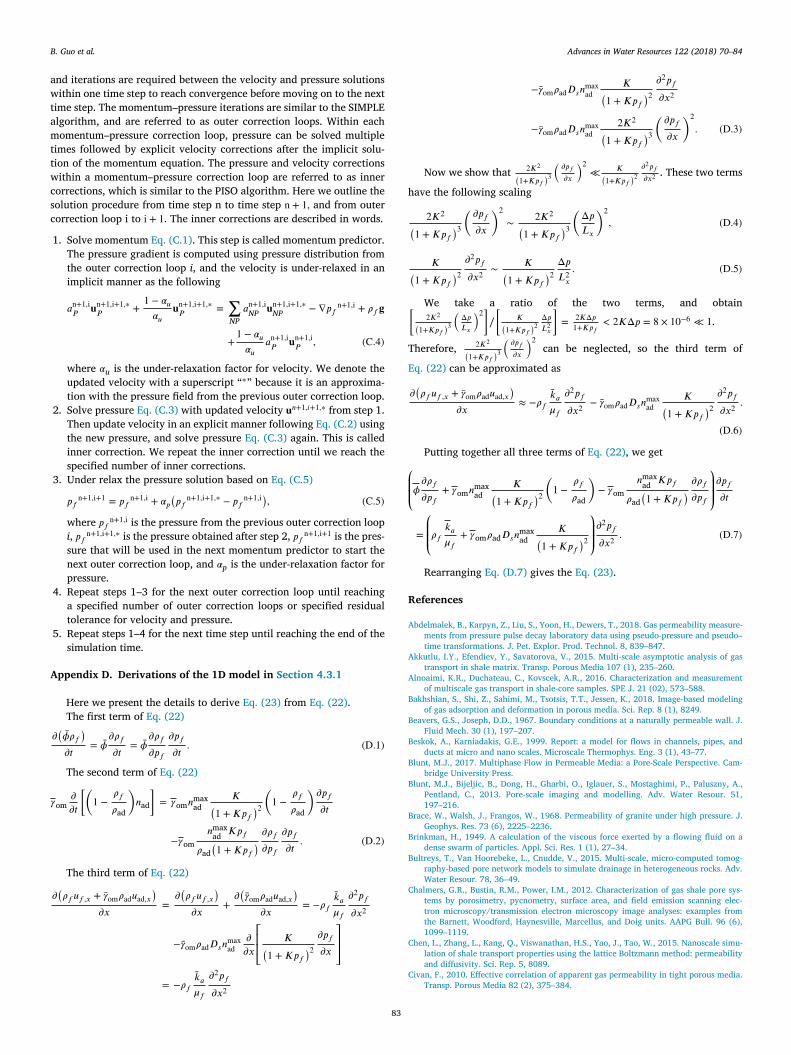
B. Guo et al. Advances in Water Resources 122 (2018) 70–84

a

w

t

a

m

t

t

w

c

s

c

A

𝛾

h

[T

E

⎛⎜⎜⎝

R

A

A

A

B

B

B

B

B

B

B

B

C

C

C

nd iterations are required between the velocity and pressure solutionsithin one time step to reach convergence before moving on to the next

ime step. The momentum–pressure iterations are similar to the SIMPLElgorithm, and are referred to as outer correction loops. Within eachomentum–pressure correction loop, pressure can be solved multiple

imes followed by explicit velocity corrections after the implicit solu-ion of the momentum equation. The pressure and velocity correctionsithin a momentum–pressure correction loop are referred to as inner

orrections, which is similar to the PISO algorithm. Here we outline theolution procedure from time step n to time step n + 1 , and from outerorrection loop i to i + 1 . The inner corrections are described in words.

1. Solve momentum Eq. (C.1) . This step is called momentum predictor.The pressure gradient is computed using pressure distribution fromthe outer correction loop i , and the velocity is under-relaxed in animplicit manner as the following

𝑎 n+1 , i 𝑃

𝐮 n+1 , i+1 , ∗ 𝑃

+

1 − 𝛼𝑢

𝛼𝑢

𝐮 n+1 , i+1 , ∗ 𝑃

=

∑NP

𝑎 n+1 , i NP

𝐮 n+1 , i+1 , ∗ NP

− ∇ 𝑝 𝑓 n+1 , i + 𝜌𝑓 𝐠

+

1 − 𝛼𝑢

𝛼𝑢

𝑎 n+1 , i 𝑃

𝐮 n+1 , i 𝑃

, (C.4)

where 𝛼u is the under-relaxation factor for velocity. We denote theupdated velocity with a superscript “∗ ” because it is an approxima-tion with the pressure field from the previous outer correction loop.

2. Solve pressure Eq. (C.3) with updated velocity 𝐮 𝑛 +1 ,𝑖 +1 , ∗ from step 1.Then update velocity in an explicit manner following Eq. (C.2) usingthe new pressure, and solve pressure Eq. (C.3) again. This is calledinner correction. We repeat the inner correction until we reach thespecified number of inner corrections.

3. Under relax the pressure solution based on Eq. (C.5)

𝑝 𝑓 n+1 , i+1 = 𝑝 𝑓

n+1 , i + 𝛼𝑝

(𝑝 𝑓

n+1 , i+1 , ∗ − 𝑝 𝑓 n+1 , i ), (C.5)

where 𝑝 𝑓 n+1 , i is the pressure from the previous outer correction loop

i , 𝑝 𝑓 n+1 , i+1 , ∗ is the pressure obtained after step 2, 𝑝 𝑓

n+1 , i+1 is the pres-sure that will be used in the next momentum predictor to start thenext outer correction loop, and 𝛼p is the under-relaxation factor forpressure.

4. Repeat steps 1–3 for the next outer correction loop until reachinga specified number of outer correction loops or specified residualtolerance for velocity and pressure.

5. Repeat steps 1–4 for the next time step until reaching the end of thesimulation time.

ppendix D. Derivations of the 1D model in Section 4.3.1

Here we present the details to derive Eq. (23) from Eq. (22) . The first term of Eq. (22)

𝜕 (��𝜌𝑓

)𝜕𝑡

= ��𝜕𝜌𝑓

𝜕𝑡 = ��

𝜕𝜌𝑓

𝜕𝑝 𝑓

𝜕𝑝 𝑓

𝜕𝑡 . (D.1)

The second term of Eq. (22)

om

𝜕

𝜕𝑡

[ (

1 −

𝜌𝑓

𝜌ad

)

𝑛 ad

] = 𝛾om

𝑛 max ad

𝐾 (1 + 𝐾𝑝 𝑓

)2 (

1 −

𝜌𝑓

𝜌ad

)

𝜕𝑝 𝑓

𝜕𝑡

− 𝛾om

𝑛 max ad

𝐾𝑝 𝑓

𝜌ad (1 + 𝐾𝑝 𝑓

) 𝜕𝜌𝑓

𝜕𝑝 𝑓

𝜕𝑝 𝑓

𝜕𝑡 . (D.2)

The third term of Eq. (22)

𝜕 (𝜌𝑓 𝑢 𝑓 ,𝑥 + 𝛾om 𝜌ad 𝑢 ad ,𝑥

)𝜕𝑥

=

𝜕 (𝜌𝑓 𝑢 𝑓 ,𝑥

)𝜕𝑥

+

𝜕 (��om 𝜌ad 𝑢 ad ,𝑥

)𝜕𝑥

= − 𝜌𝑓

�� 𝑎 𝜇𝑓

𝜕 2 𝑝 𝑓

𝜕𝑥 2

− 𝛾om 𝜌ad 𝐷 𝑠 𝑛 max ad

𝜕

𝜕𝑥

⎡ ⎢ ⎢ ⎣ 𝐾 (1 + 𝐾𝑝 𝑓

)2 𝜕𝑝 𝑓

𝜕𝑥

⎤ ⎥ ⎥ ⎦ = − 𝜌𝑓

�� 𝑎 𝜇𝑓

𝜕 2 𝑝 𝑓

𝜕𝑥 2

83

− 𝛾om 𝜌ad 𝐷 𝑠 𝑛 max ad

𝐾 (1 + 𝐾𝑝 𝑓

)2 𝜕 2 𝑝 𝑓 𝜕𝑥 2

− 𝛾om 𝜌ad 𝐷 𝑠 𝑛 max ad

2 𝐾

2 (1 + 𝐾𝑝 𝑓

)3 (

𝜕𝑝 𝑓

𝜕𝑥

) 2 . (D.3)

Now we show that 2 𝐾 2 (1+ 𝐾𝑝 𝑓

)3 ( 𝜕𝑝 𝑓

𝜕𝑥

)2 ≪

𝐾 (1+ 𝐾𝑝 𝑓

)2 𝜕 2 𝑝 𝑓 𝜕𝑥 2 . These two terms

ave the following scaling

2 𝐾

2 (1 + 𝐾𝑝 𝑓

)3 (

𝜕𝑝 𝑓

𝜕𝑥

) 2 ∼ 2 𝐾

2 (1 + 𝐾𝑝 𝑓

)3 (

Δ𝑝

𝐿 𝑥

) 2 , (D.4)

𝐾 (1 + 𝐾𝑝 𝑓

)2 𝜕 2 𝑝 𝑓 𝜕𝑥 2 ∼ 𝐾 (

1 + 𝐾𝑝 𝑓 )2 Δ𝑝

𝐿

2 𝑥

. (D.5)

We take a ratio of the two terms, and obtain

2 𝐾 2 (1+ 𝐾𝑝 𝑓

)3 ( Δ𝑝

𝐿 𝑥

)2 ] ∕ [

𝐾 (1+ 𝐾𝑝 𝑓

)2 Δ𝑝

𝐿 2 𝑥

] =

2 𝐾Δ𝑝

1+ 𝐾𝑝 𝑓 < 2 𝐾Δ𝑝 = 8 × 10 −6 ≪ 1 .

herefore, 2 𝐾 2 (1+ 𝐾𝑝 𝑓

)3 ( 𝜕𝑝 𝑓

𝜕𝑥

)2 can be neglected, so the third term of

q. (22) can be approximated as

𝜕 (𝜌𝑓 𝑢 𝑓 ,𝑥 + 𝛾om 𝜌ad 𝑢 ad ,𝑥

)𝜕𝑥

≈ − 𝜌𝑓

�� 𝑎 𝜇𝑓

𝜕 2 𝑝 𝑓

𝜕𝑥 2 − 𝛾om 𝜌ad 𝐷 𝑠 𝑛

max ad

𝐾 (1 + 𝐾𝑝 𝑓

)2 𝜕 2 𝑝 𝑓 𝜕𝑥 2 .

(D.6)

Putting together all three terms of Eq. (22) , we get

𝜙𝜕𝜌𝑓

𝜕𝑝 𝑓 + 𝛾om

𝑛 max ad

𝐾 (1 + 𝐾𝑝 𝑓

)2 (

1 −

𝜌𝑓

𝜌ad

)

− 𝛾om

𝑛 max ad

𝐾𝑝 𝑓

𝜌ad (1 + 𝐾𝑝 𝑓

) 𝜕𝜌𝑓

𝜕𝑝 𝑓

⎞ ⎟ ⎟ ⎠ 𝜕𝑝 𝑓

𝜕𝑡

=

⎛ ⎜ ⎜ ⎝ 𝜌𝑓

𝑘 𝑎 𝜇𝑓

+ 𝛾om

𝜌ad 𝐷 𝑠 𝑛 max ad

𝐾 (1 + 𝐾𝑝 𝑓

)2 ⎞ ⎟ ⎟ ⎠ 𝜕 2 𝑝 𝑓

𝜕𝑥 2 . (D.7)

Rearranging Eq. (D.7) gives the Eq. (23) .

eferences

bdelmalek, B. , Karpyn, Z. , Liu, S. , Yoon, H. , Dewers, T. , 2018. Gas permeability measure-ments from pressure pulse decay laboratory data using pseudo-pressure and pseudo–time transformations. J. Pet. Explor. Prod. Technol. 8, 839–847 .

kkutlu, I.Y. , Efendiev, Y. , Savatorova, V. , 2015. Multi-scale asymptotic analysis of gastransport in shale matrix. Transp. Porous Media 107 (1), 235–260 .

lnoaimi, K.R. , Duchateau, C. , Kovscek, A.R. , 2016. Characterization and measurementof multiscale gas transport in shale-core samples. SPE J. 21 (02), 573–588 .

akhshian, S. , Shi, Z. , Sahimi, M. , Tsotsis, T.T. , Jessen, K. , 2018. Image-based modelingof gas adsorption and deformation in porous media. Sci. Rep. 8 (1), 8249 .

eavers, G.S. , Joseph, D.D. , 1967. Boundary conditions at a naturally permeable wall. J.Fluid Mech. 30 (1), 197–207 .

eskok, A. , Karniadakis, G.E. , 1999. Report: a model for flows in channels, pipes, andducts at micro and nano scales. Microscale Thermophys. Eng. 3 (1), 43–77 .

lunt, M.J. , 2017. Multiphase Flow in Permeable Media: a Pore-Scale Perspective. Cam-bridge University Press .

lunt, M.J. , Bijeljic, B. , Dong, H. , Gharbi, O. , Iglauer, S. , Mostaghimi, P. , Paluszny, A. ,Pentland, C. , 2013. Pore-scale imaging and modelling. Adv. Water Resour. 51,197–216 .

race, W. , Walsh, J. , Frangos, W. , 1968. Permeability of granite under high pressure. J.Geophys. Res. 73 (6), 2225–2236 .

rinkman, H. , 1949. A calculation of the viscous force exerted by a flowing fluid on adense swarm of particles. Appl. Sci. Res. 1 (1), 27–34 .

ultreys, T. , Van Hoorebeke, L. , Cnudde, V. , 2015. Multi-scale, micro-computed tomog-raphy-based pore network models to simulate drainage in heterogeneous rocks. Adv.Water Resour. 78, 36–49 .

halmers, G.R. , Bustin, R.M. , Power, I.M. , 2012. Characterization of gas shale pore sys-tems by porosimetry, pycnometry, surface area, and field emission scanning elec-tron microscopy/transmission electron microscopy image analyses: examples fromthe Barnett, Woodford, Haynesville, Marcellus, and Doig units. AAPG Bull. 96 (6),1099–1119 .

hen, L. , Zhang, L. , Kang, Q. , Viswanathan, H.S. , Yao, J. , Tao, W. , 2015. Nanoscale simu-lation of shale transport properties using the lattice Boltzmann method: permeabilityand diffusivity. Sci. Rep. 5, 8089 .

ivan, F. , 2010. Effective correlation of apparent gas permeability in tight porous media.Transp. Porous Media 82 (2), 375–384 .

B. Guo et al. Advances in Water Resources 122 (2018) 70–84

C

C

C

D

D

E

EG

G

H

H

I

J

J

J

K

K

K

L

L

L

L

M

M

M

M

M

M

M

M

PR

R

R

R

S

S

S

S

S

W

W

W

W

W

X

Z

larkson, C.R. , Solano, N. , Bustin, R.M. , Bustin, A. , Chalmers, G. , He, L. , Mel-nichenko, Y.B. , Radli ń ski, A. , Blach, T.P. , 2013. Pore structure characterization ofNorth American shale gas reservoirs using USANS/SANS, gas adsorption, and mer-cury intrusion. Fuel 103, 606–616 .

ui, X. , Bustin, A. , Bustin, R.M. , 2009. Measurements of gas permeability and diffusivityof tight reservoir rocks: different approaches and their applications. Geofluids 9 (3),208–223 .

urtis, M.E. , Sondergeld, C.H. , Ambrose, R.J. , Rai, C.S. , 2012. Microstructural investi-gation of gas shales in two and three dimensions using nanometer-scale resolutionimaging. AAPG Bull. 96 (4), 665–677 .

arabi, H. , Ettehad, A. , Javadpour, F. , Sepehrnoori, K. , 2012. Gas flow in ultra-tight shalestrata. J. Fluid Mech. 710, 641–658 .

icker, A. , Smits, R. , 1988. A practical approach for determining permeability from labora-tory pressure-pulse decay measurements. In: Proceedings of the International Meetingon Petroleum Engineering. Society of Petroleum Engineers .

dwards, R.W. , Celia, M.A. , Bandilla, K.W. , Doster, F. , Kanno, C.M. , 2015. A model toestimate carbon dioxide injectivity and storage capacity for geological sequestrationin shale gas wells. Environ. Sci. Technol. 49 (15), 9222–9229 .

IA , 2017. Natural Gas Annual Report. U.S. Energy Information Administration . ensterblum, Y. , Ghanizadeh, A. , Cuss, R.J. , Amann-Hildenbrand, A. , Krooss, B.M. , Clark-

son, C.R. , Harrington, J.F. , Zoback, M.D. , 2015. Gas transport and storage capacity inshale gas reservoirs–a review. Part A: transport processes. J. Unconv. Oil Gas Resour.12, 87–122 .

oyeau, B. , Lhuillier, D. , Gobin, D. , Velarde, M. , 2003. Momentum transport at a fluid—porous interface. Int. J. Heat Mass Transf. 46 (21), 4071–4081 .

eller, R. , Vermylen, J. , Zoback, M. , 2014. Experimental investigation of matrix perme-ability of gas shales. AAPG Bull. 98 (5), 975–995 .

eller, R. , Zoback, M. , 2014. Adsorption of methane and carbon dioxide on gas shale andpure mineral samples. J. Unconv. Oil Gas Resour. 8, 14–24 .

ssa, R.I. , 1986. Solution of the implicitly discretised fluid flow equations by operator-s-plitting. J. Comput. Phys. 62 (1), 40–65 .

asak, H. , 1996. Error Analysis and Estimation for the Finite Volume Method with Appli-cations to Fluid Flows. University of London Imperial College Ph.D. thesis .

avadpour, F. , 2009. Nanopores and apparent permeability of gas flow in mudrocks (shalesand siltstone). J. Can. Pet. Technol. 48 (08), 16–21 .

ones, S. , 1997. A technique for faster pulse-decay permeability measurements in tightrocks. SPE Form. Eval. 12 (01), 19–26 .

arniadakis, G.E. , Beskok, A. , Aluru, N. , 2005. Microflows and Nanoflows: Fundamentalsand Simulation. Springer .

elly, S. , El-Sobky, H. , Torres-Verdín, C. , Balhoff, M.T. , 2016. Assessing the utility ofFIB-SEM images for shale digital rock physics. Adv. Water Resour. 95, 302–316 .

linkenberg, L. , 1941. The permeability of porous media to liquids and gases. Drilling andProduction Practice. American Petroleum Institute .

andry, C.J. , Prodanovi ć, M. , Eichhubl, P. , 2016. Direct simulation of supercritical gasflow in complex nanoporous media and prediction of apparent permeability. Int. J.Coal Geol. 159, 120–134 .

ee, A.L. , Gonzalez, M.H. , Eakin, B.E. , 1966. The viscosity of natural gases. J. Pet. Technol.18 (08), 997–1000 .

emmon, E. , McLinden, M. , Friend., D. , 1998. Thermophysical properties of fluid systems.In: Linstrom, P., Mallard, W. (Eds.), NIST Chemistry WebBook, NIST Standard Refer-ence Database Number 69. National Institute of Standards and Technology, Gaithers-burg MD .

unati, I. , Lee, S. , 2014. A dual-tube model for gas dynamics in fractured nanoporous shaleformations. J. Fluid Mech. 757, 943–971 .

a, L. , Fauchille, A.-L. , Dowey, P.J. , Pilz, F.F. , Courtois, L. , Taylor, K.G. , Lee, P.D. , 2017.Correlative multi-scale imaging of shales: a review and future perspectives. Geol. Soc.Lond. Spec. Publ. 454 (1), 175–199 .

a, L. , Slater, T. , Dowey, P.J. , Yue, S. , Rutter, E.H. , Taylor, K.G. , Lee, P.D. , 2018. Hierar-chical integration of porosity in shales. Sci. Rep. 8 (1), 11683 .

84

a, L. , Taylor, K.G. , Lee, P.D. , Dobson, K.J. , Dowey, P.J. , Courtois, L. , 2016. Novel 3D cen-timetre-to nano-scale quantification of an organic-rich mudstone: the CarboniferousBowland Shale, Northern England. Mar. Pet. Geol. 72, 193–205 .

ahmoud, M. , 2014. Development of a new correlation of gas compressibility factor (Z–factor) for high pressure gas reservoirs. J. Energy Resour. Technol. 136 (1), 012903 .

ason, E.A. , Malinauskas, A. , 1983. Gas Transport in Porous Media: the Dusty-Gas Model,17. Elsevier Science Ltd .

edve ď, I. , Čern ỳ, R. , 2011. Surface diffusion in porous media: a critical review. Microp-orous Mesoporous Mater. 142 (2), 405–422 .

ehmani, A. , Prodanovi ć, M. , 2014. The effect of microporosity on transport propertiesin porous media. Adv. Water Resour. 63, 104–119 .

ehmani, A. , Prodanovi ć, M. , Javadpour, F. , 2013. Multiscale, multiphysics network mod-eling of shale matrix gas flows. Transp. Porous Media 99 (2), 377–390 .

atankar, S. , 1980. Numerical Heat Transfer and Fluid Flow. CRC press . exer, T.F. , Mathia, E.J. , Aplin, A.C. , Thomas, K.M. , 2014. High-pressure methane adsorp-

tion and characterization of pores in Posidonia shales and isolated kerogens. EnergyFuels 28 (5), 2886–2901 .

oss, D.J. , Bustin, R.M. , 2009. The importance of shale composition and pore struc-ture upon gas storage potential of shale gas reservoirs. Mar. Pet. Geol. 26 (6), 916–927 .

ouquerol, J. , Avnir, D. , Fairbridge, C. , Everett, D. , Haynes, J. , Pernicone, N. , Ramsay, J. ,Sing, K. , Unger, K. , 1994. Recommendations for the characterization of porous solids(technical report). Pure Appl. Chem. 66 (8), 1739–1758 .

uthven, D.M. , 1984. Principles of Adsorption and Adsorption Processes. John Wiley &Sons .

akhaee-Pour, A. , Bryant, S. , 2012. Gas permeability of shale. SPE Reserv. Eval. Eng. 15(04), 401–409 .

cheibe, T.D. , Perkins, W.A. , Richmond, M.C. , McKinley, M.I. , Romero-Gomez, P.D. , Oost-rom, M. , Wietsma, T.W. , Serkowski, J.A. , Zachara, J.M. , 2015. Pore-scale and multi-scale numerical simulation of flow and transport in a laboratory-scale column. WaterResour. Res. 51 (2), 1023–1035 .

ondergeld, C.H. , Ambrose, R.J. , Rai, C.S. , Moncrieff, J. , 2010. Micro-structural studiesof gas shales. In: Proceedings of the SPE Unconventional Gas Conference. Society ofPetroleum Engineers .

ong, W. , Yao, J. , Ma, J. , Couples, G. , Li, Y. , 2017. Assessing relative contributions oftransport mechanisms and real gas properties to gas flow in nanoscale organic poresin shales by pore network modelling. Int. J. Heat Mass Transf. 113, 524–537 .

oulaine, C. , Tchelepi, H.A. , 2016. Micro-continuum approach for pore-scale simulationof subsurface processes. Transp. Porous Media 113 (3), 431–456 .

ang, J. , Chen, L. , Kang, Q. , Rahman, S.S. , 2016. The lattice Boltzmann method forisothermal micro-gaseous flow and its application in shale gas flow: a review. Int.J. Heat Mass Transf. 95, 94–108 .

ang, J. , Kang, Q. , Chen, L. , Rahman, S.S. , 2017. Pore-scale lattice Boltzmann simula-tion of micro-gaseous flow considering surface diffusion effect. Int. J. Coal Geol. 169,62–73 .

u, K. , Li, X. , Guo, C. , Wang, C. , Chen, Z. , 2016. A unified model for gas transfer innanopores of shale-gas reservoirs: coupling pore diffusion and surface diffusion. SPEJ. 21 (05), 1–583 .

u, T. , Li, X. , Zhao, J. , Zhang, D. , 2017. Mutiscale pore structure and its effect on gastransport in organic-rich shale. Water Resour. Res. 53, 5438–5450 .

u, T. , Zhang, D. , 2016. Impact of adsorption on gas transport in nanopores. Sci. Rep. 6,23629 .

iong, X. , Devegowda, D. , Villazon, M. , German, G. , Sigal, R.F. , Civan, F. , 2012. A fully–coupled free and adsorptive phase transport model for shale gas reservoirs includingnon-darcy flow effects. In: Proceedings of the SPE Annual Technical Conference andExhibition. Society of Petroleum Engineers .

hang, T. , Ellis, G.S. , Ruppel, S.C. , Milliken, K. , Yang, R. , 2012. Effect of organic-mat-ter type and thermal maturity on methane adsorption in shale-gas systems. Org.Geochem. 47, 120–131 .