FACULTY OF ENGINEERING OF THE UNIVERSITY OF PORTO DEPARTMENT OF ELECTRICAL AND COMPUTER ENGINEERING

Advances on the Sequential Monte Carlo Reliability Assessment of Generation-

Transmission Systems using Cross-Entropy and Population-based Methods

Leonel de Magalhães Carvalho, M.Sc.

THESIS SUBMITTED TO THE FACULTY OF ENGINEERING OF THE UNIVERSITY OF

PORTO IN PARTIAL FULFILLMENT OF THE REQUIREMENTS FOR THE DEGREE OF

DOCTOR OF PHILOSOPHY

Supervisor: Professor Vladimiro Henrique Barrosa Pinto de Miranda, Ph.D. Co-supervisor: Mauro Augusto da Rosa, Ph.D.

Porto, Portugal June, 2013

© Leonel de Magalhães Carvalho, 2013

i

This work was supported by the Portuguese Foundation for Science and Technology (FCT) under the grant SFRH/BD/43004/2008 and by the Institute for Systems and Computer Engineering of Porto (coordinating entity of INESC TEC).

ii

iii

What I cannot create, I do not understand. (Richard P. Feynman)

iv

v

Acknowledgments

I start this list of acknowledgments by expressing my sincere gratitude to my supervisor, Professor Doctor Vladimiro Henrique Barrosa Pinto de Miranda, for the refinement of this work, for his key insights, for his cheerful encouragement, for being a person open to new ideas, and, most of all, for giving me the opportunity to pursuit my research interests and ideas throughout this overwhelming but rewarding journey.

I am also most grateful to my co-supervisor, Professor Mauro Augusto da Rosa, whose hard work, unconditional availability, never-ending patience, and scientific guidance has not only helped me to conclude this work but also how to be a less amateurish researcher. Throughout the time we have been working together, he has wisely advised me in the delicate balance between personal objectives and research interests. Today we are not only actively cooperating peers but also cherished friends.

Next, I address a special thanks to Professor Armando Leite da Silva. To work with such an enlightened, brilliant and competent scientist is indeed a once-in-a-life-time opportunity. During the 6 months I had the privilege to collaborate with him, I expanded my knowledge in the field of power systems reliability assessment in such an effortless way that even today I am amazed at how was I even able to do it. Most of the work that led to Chapter 4 was inspired by his award-winning achievements over the past four years. I will always be grateful for the knowledge Professor Leite da Silva has kindly passed onto me.

During the past 5 years I have met a countless number of inspiring people that, in a way or another, have shaped this work and my perception regarding scientific accomplishment. Among these people, none have been more influential than Diego Issicaba, Hrvoje Keko, Reinaldo Andrés González-Fernández and Jean Akilimali Sumaili. I thank you very much for everything you have taught me.

For the excellent working environment, I must acknowledge the people who were or are part of the Power Systems Unit of INESC Porto, namely, Leonardo Bremermann, Jakov Opara, Joel Ramos, Ivo Costa, Bernardo Silva, Pedro Almeida, Joel Soares, Luís Seca, André Madureira, Paula Castro, Professor Carlos Moreira and Professor Manuel Matos. Special thanks are addressed to Rute Ferreira as she has been a close friend ever since the first day I joined this research institution.

In Brazil I was hosted at the Institute of Electric Systems and Energy, Federal University of Itajubá, Minas Gerais. In this laboratory I found remarkable people that made everything possibly to make me feel like home. For their kind friendship, I thank Luís Lima, Silvan Flávio, Diogo Marujo, Marcos Santos, Janaina Costa, Adriano Almeida, Denisson Oliveira, Aurélio Coelho and Marcus Sollyvan. I am also indebted to those that

vi

made my stay in Brazil an unforgettable experience, namely, José Issicaba, Dalva Magro, Edson Moreira, and Kelly Cappellesso.

Above all, I am grateful to my family. In particular, I thank my father, Manuel da Rocha Carvalho, my mother, Maria da Conceição de Oliveira Magalhães, and my brother, Nuno Filipe Magalhães Carvalho, for their love and affection, for believing in me, for their persistent support, for giving me the opportunity to improve my education, for all their sacrifices, for stoically enduring my absence when I was abroad, and, above all, for instilling in me the value of honest work. From the bottom of my heart, I thank you very much.

This list of acknowledgements is not complete until I make a reference to one of the best human beings I have ever met: my beloved girlfriend Ana Catarina Moreira de Carvalho Rola. Her care, tolerance, understanding, presence, support, enthusiasm, and, most of all, her unconditional love were decisive for me to finish this dissertation.

I end this list of acknowledgments by thanking the secretariat of the Doctoral Program in Sustainable Energy Systems (PDSSE), the director of the PDSSE, Professor João Abel Peças Lopes, and the director of the Faculty of Engineering of the University of Porto (FEUP), Professor Sebastião José Cabral Feyo de Azevedo. I am also grateful for the funding provided by the Portuguese Foundation for Science and Technology (FCT) and by INESC TEC (coordinating entity of INESC Porto).

vii

Abstract

The sequential Monte Carlo simulation (MCS) method is one of the most powerful tools for power systems adequacy assessment. By sequentially sampling the duration of the states, this method can inherently incorporate the stochastic behavior of the system components, time-dependent issues like the renewable power production, reservoir operating rules, scheduled maintenance, complex correlated load models, etc. Moreover, it can provide unique results, such as the probability distribution of the reliability indices. Despite these advantages, the simulation time of the sequential MCS method is seen as its major weakness. Hence, the main objectives of this dissertation are to investigate and propose algorithmic advances that can effectively improve the time-efficiency of the sequential MCS method applied to the adequacy assessment of the generating capacity and composite (generation and transmission) system.

This dissertation is structurally divided into three parts. Taking advantage of the flexibility of the sequential MCS method developed in the scope of this dissertation, the first part has analyzed the impacts that a growing integration of wind power can have on the adequacy of the composite system. More specifically, the sequential MCS method was used to detect the loss of load and wind curtailment events. The categorization of the different wind power curtailment events was made according to a simple algorithm. Moreover, the dispatch rules of the generating units when a large share of the generating capacity is intermittent were considered in the analysis through a simple model. The dual variables of the DC Optimal Power Flow were also exploited help identify which transmission circuits are restricting the use of the total wind power available. Case studies based on the IEEE-RTS 79 system were made to shed light on the impacts that different generation technologies, namely wind and thermal units, can have on the adequacy of the composite system. The results of these case studies showed that the comparison between these two generation technologies depends on the performance criterion and on the reliability index selected. Wind power curtailment events under a strategy of maximum use of wind power were also investigated. In this case, the experiments have demonstrated that the transmission network may not limit the use of wind power as severely as the dispatch rules of the system operator.

The second part of this dissertation has explored the application of the Cross-Entropy (CE) method and the Importance Sampling (IS) variance reduction technique in the sequential MCS method. A new algorithm was proposed to calculate the CE-optimal IS distribution for the generating capacity adequacy assessment. This new CE-based algorithm steams from the mathematical analysis of the CE equations that has demonstrated that the CE-optimal IS distribution can be obtained by simply dividing the annualized reliability

viii

indices for different configurations of the generating system. The results of the application of the new CE-based algorithm to the generating systems of the IEEE-RTS 79, IEEE-RTS 96, and two configurations of the Brazilian South-Southeastern system have shown that this algorithm, whose core is the fast Fourier transform, is equivalent to the standard CE optimization algorithm in accuracy and computational effort. The relevant feature of the new CE-based algorithm when compared to the standard CE optimization algorithm is its simplicity of implementation. Several strategies for modeling the generating units with time-dependent capacity in the CE-based algorithms were also suggested and their impact on the simulation time duly analyzed. The second part of this dissertation has also proposed and examined a CE optimization algorithm for the composite system adequacy assessment.

The third part of this dissertation has introduced the innovative application of a Population-Based method (PBM) to improve the efficiency of the sequential MCS method. The proposed methodology consists of two phases. Firstly, a list of high probability states that cannot supply the peak load is created by a PBM. The PBM used takes advantage of the space-covering characteristics of the Evolutionary Particle Swarm Optimization (EPSO) metaheuristic. Secondly, the states sampled by the sequential MCS method are compared to those on the list to decide whether full evaluation should be performed or not. If a state proceeds to evaluation, the yearly load model, the time-dependency of the capacity of the generating units, and other chronological features are sequentially followed to form system states. These system states may or may not have loss of load. If the state sampled is not in the list, then it is assumed that no loss of load occurs throughout its duration. The proposed methodology was applied to the adequacy assessment of the generating capacity and the composite system of configurations of the IEEE-RTS 79 and IEEE-RTS 96 systems that include hydro and wind intermittency.

The results obtained from using the CE method and IS in the sequential MCS method reported remarkable speed ups in the estimation of the reliability indices for the generating capacity and composite system (in some experiments, the time gain over the crude sequential MCS method is more than 60 times). Moreover, it was observed that the speed up increases as the system becomes more reliable. Unfortunately, the sequential MCS method cannot provide accurate probability distributions for the reliability indices if the CE method and IS are used. On the other hand, the experiments carried out in the third part of this dissertation demonstrated that the speed ups achieved are only comparable to the ones obtained by the CE method and IS if the system is unreliable. Despite this disadvantage, this methodology can obtain accurate probability distributions for the reliability indices if the classification process does not fail to detect the states that need evaluation.

ix

Resumo

O método sequencial de simulação de Monte Carlo (SMC) é uma das ferramentas mais poderosas para a avaliação da adequação dos sistemas elétricos de energia. Através da amostragem sequencial da duração dos estados, este método pode incluir naturalmente o comportamento estocástico dos componentes do sistema, a intermitência dos recursos de energia renovável, as regras de operação dos reservatórios das centrais hídricas, a manutenção programada das unidades de geração, a variação horária da carga, etc. Além disso, este método pode fornecer resultados únicos, tais como a distribuição de probabilidade dos índices de fiabilidade. Apesar destas vantagens, o tempo de execução do método sequencial de SMC é visto como a sua maior desvantagem. Perante este facto, os principais objetivos desta tese consistem na investigação e desenvolvimento de avanços algorítmicos para melhorar a eficiência da execução do método sequencial de SMC na avaliação da adequação do sistema de geração e do sistema composto (geração e transmissão).

Estruturalmente, esta dissertação foi dividida em três partes. Aproveitando a flexibilidade do método sequencial de SMC desenvolvido no âmbito desta tese, a primeira parte analisou os impactos que a integração gradual de energia eólica pode ter na adequação do sistema composto. Por conseguinte, o método sequencial de SMC foi utilizado para detetar os eventos de corte de carga e os eventos de desperdício de potência eólica. Para categorizar os diferentes eventos de desperdício de potência eólica, um algoritmo simples foi proposto. Além disso, as preferências dos operadores do sistema no despacho das unidades de geração quando uma grande parte da capacidade de geração é intermitente também foram consideradas na análise. As variáveis duais do Transito de Potências Ótimo DC foram exploradas para identificar quais os circuitos da rede de transporte que restringem o uso da toda a energia eólica disponível. Estudos de caso baseados no sistema IEEE-RTS 79 foram realizados para determinar o impacto que as diferentes tecnologias de geração têm, nomeadamente térmica e eólica, na adequação do sistema composto. Os resultados obtidos destes casos de estudo demonstraram que o resultado da comparação entre estas duas tecnologias depende do critério de desempenho e do índice de fiabilidade selecionado. Os eventos de desperdício de potência eólica numa estratégia de maximização do uso de energia eólica foram também investigados. Neste caso, as experiências demonstraram que a rede de transporte pode não restringir o uso de energia eólica tão severamente como as preferências de despacho utilizadas pelo operador do sistema.

A segunda parte desta tese explorou a aplicação do método de Entropia Cruzada (EC) e da técnica de redução de variância de Amostragem por Importância (AI) no método sequencial de SMC. Desta forma, um novo algoritmo para calcular a distribuição ótima da

x

técnica de AI para o problema da avaliação da adequação da capacidade de geração foi proposto. Este algoritmo é baseado na análise das equações do método de EC. Desta análise demostrou-se que a distribuição ótima da técnica de AI pode ser calculada de uma forma simples através da divisão dos índices de fiabilidade anualizados de diferentes configurações do sistema de geração. A aplicação do método proposto na análise da adequação dos sistemas de geração do IEEE-RTS 79, IEEE-RTS 96, e duas configurações do sistema Su-sudeste brasileiro demonstrou que o novo algoritmo, cujo núcleo é a transformada rápida de Fourier, é equivalente ao algoritmo de otimização padrão do método de EC tanto na precisão dos resultados como no desempenho computacional. Claramente, a característica inovadora do novo algoritmo é a sua simplicidade de implementação. A segunda parte desta tese propõe também um algoritmo de otimização baseado no método de EC para a avaliação da adequação do sistema composto. Além disso, várias estratégias para modelizar as unidades de geração cuja capacidade depende do tempo foram sugeridas e o respetivo impacto sobre o tempo de simulação do método sequencial de SMC foi devidamente analisado.

A terceira parte da tese introduziu a utilização de um método de base populacional (MBP) para a diminuição do tempo de simulação do método sequencial de SMC. A metodologia proposta consiste em duas fases. Em primeiro lugar, uma lista de estados com alta probabilidade de ocorrência e que são incapazes de suprir a ponta da carga é criada por um MBP. O MBP utilizado aproveita as excelentes características do método evolucionário de Enxame de Partículas (EPSO) para se efetuar uma cobertura abrangente do espaço de pesquisa. Em segundo lugar, os estados amostrados pelo método sequencial de SMCS são comparados com os da lista para se decidir se uma avaliação completa deve ser realizada ou não. Caso o estado amostrado necessite de uma avaliação completa, o modelo de carga anual, a variação temporal da capacidade das unidades de geração e outras características cronológicas são sequencialmente seguidas para formar estados de sistema. Estes estados de sistema podem ou não ter corte de carga. Se o estado amostrado não está na lista, então assume-se que não ocorre corte de carga ao longo da toda a sua duração. A metodologia proposta foi aplicada na avaliação da adequação da capacidade de geração e do sistema composto de configurações dos sistemas IEEE-RTS 79 e IEEE-RTS 96 que incluem a intermitência dos recursos hidrológicos e eólicos.

Finalmente, os resultados obtidos da utilização do método de EC e da técnica de AI no método sequencial de SMC revelaram ganhos notáveis no tempo necessário para obter estimativas dos índices de fiabilidade para o sistema de geração e para o sistema composto (nalgumas experiências, o ganho sobre o método sequencial de SMC tradicional é superior a 60 vezes). Estes resultados mostraram também que os ganhos em tempo de simulação aumentam consideravelmente à medida que o sistema se torna mais fiável. Infelizmente, as distribuições de probabilidade dos índices de fiabilidade não são obtidas se técnicas de redução de variância, como a AI, forem utilizadas. Por outro lado, as experiências levadas a cabo na terceira parte desta dissertação demonstraram que a aceleração do tempo de execução do método sequencial de SMC obtida por esta abordagem é somente comparável com aquela obtida pela utilização do método de EC e a técnica de AI se o sistema não é fiável. Por outro lado, uma vez que esta abordagem baseia-se num processo de

xi

classificação e não em técnicas de redução de variância, é possível obter distribuições de probabilidade para os índices de fiabilidade caso o processo de classificação não cometa erros significativos na deteção dos estados que necessitam de uma avaliação completa.

xii

xiii

Résumé

La méthode de simulation de Monte Carlo (SMC) séquentielle est un des outils les plus puissants pour l'évaluation de l'adéquation des systèmes électriques d'énergie. À travers l'échantillonnage séquentiel de la durée des états, cette méthode peut inclure naturellement le comportement aléatoire des composantes du système, l'intermittence des ressources d'énergie renouvelable, les règles d'opération des réservoirs des centrales hydro-électriques, la manutention programmée des unités de génération, la variation horaire de la charge, etc. En outre, cette méthode peut fournir des résultats uniques comme la distribution de probabilité des indices de fiabilité. Malgré ces avantages, le temps d'exécution de la méthode de SMC séquentielle est considéré comme son plus grand désavantage. Ceci étant, les principaux objectifs de cette thèse consistent à la recherche et au développement d'améliorations algorithmiques pour réduire le temps d'exécution de la méthode de SMC séquentielle dans l'évaluation de l'adéquation du système de génération et du système composé (génération et transmission).

Structurellement, cette dissertation a été divisée en trois parties. En profitant de la flexibilité de la méthode de SMC séquentielle développée dans le contexte de cette thèse, la première partie a analysé les impacts que l'intégration graduelle d'énergie éolienne peut avoir sur l'adéquation du système composé. Par conséquent, la méthode de SMC séquentielle a été utilisée pour détecter les événements de perte de charge et les événements de réduction de la puissance éolienne. Pour catégoriser les différents événements de réduction de la puissance éolienne, un algorithme simple a été proposé. En outre, les préférences des opérateurs du système, dans la décision des unités de génération quand une grande partie de la capacité de génération est intermittente, ont aussi été considérées dans l'analyse. Les variables duelles du problème d’écoulement des charges optimisé selon le modèle CC ont été exploitées pour identifier les branches du réseau de transport qui restreignent l'utilisation de la toute l'énergie éolienne disponible. Des études de cas basées sur le système IEEE-RTS 79 ont été réalisées pour déterminer l'impact que les différentes technologies de génération, notamment thermique et éolienne, ont sur l'adéquation du système composé. Les résultats obtenus de ces études de cas ont démontré que la comparaison entre ces deux technologies dépend du critère de performance et de l'indice de fiabilité choisi. Les événements de réduction de la puissance éolienne dans une stratégie de maximisation de l'utilisation de l'énergie éolienne ont aussi été explorés. Dans ce cas, les expériences ont démontré que le réseau de transport peut ne pas restreindre l'utilisation de l'énergie éolienne aussi sévèrement que les préférences de décision utilisées par l'opérateur du système.

xiv

La deuxième partie de cette dissertation a exploré l'application de la méthode d’Entropie Croisée (EC) et la technique de réduction de la variance d’Échantillonnage d’Importance (EI) dans la méthode de SMC séquentielle. Un nouvel algorithme pour calculer la distribution optimale de la technique de l’EI pour le problème d’évaluation de l’adéquation de la capacité de génération a été proposé. Ce nouvel algorithme est basé sur l’analyse des équations de la méthode d’EC. Cette analyse a démontré que la distribution optimale de la technique de l’EI peut être obtenue simplement en divisant les indices annualisés de fiabilité pour les différentes configurations du système de génération. Les résultats de l'application du nouvel algorithme basé sur l’EC aux systèmes de génération des configurations de IEEE-RTS 79, IEEE-RTS 96, et de deux configurations du système du Sud-sud-est brésilien ont prouvé que cet algorithme, dont le noyau est la transformée rapide de Fourier, est équivalent à l'algorithme standard d'optimisation de l’EC en termes de précision et d'effort de calcul. En effet, comparé à l’algorithme d’optimisation standard basé sur l’EC, le principal atout du nouvel algorithme est sa simplicité d’implémentation. Plusieurs stratégies de représentation des unités de génération dont la capacité varie dans le temps dans les algorithmes basés sur l’EC ont été également suggérées et leur impact sur le temps de simulation a été dûment analysé. La deuxième partie de cette dissertation a également proposé et a examiné un algorithme d'optimisation de l’EC pour l'évaluation de l’'adéquation de système composé.

La troisième partie de cette dissertation a présenté l'application innovatrice d'une méthode basée sur les populations (MBP) pour améliorer l'efficacité de la méthode de SMC séquentielle. La méthodologie proposée est composée de deux phases. Premièrement, une liste d’états, avec probabilité élevée, qui ne peuvent pas alimenter la charge de pointe est créée par une MBP. La MBP utilisée exploite les excellentes capacités de la méthode évolutionnaire d’Essaim de Particules (EPSO) pour effectuer une couverture de l'espace de recherche. En second lieu, les états échantillonnés par la méthode SMC séquentielle sont comparés à ceux de la liste pour décider si une évaluation complète devrait être effectuée ou pas. Si un état a besoin de subir une évaluation complète, le modèle annuel de la charge, la variation dans le temps de la capacité des unités de génération et d'autres caractéristiques chronologiques sont séquentiellement suivis pour former les états de système. Ces états peuvent ou ne pas avoir la perte de charge. Si l'état échantillonné n'est pas dans la liste, alors on suppose qu'aucune perte de charge ne se produira durant toute sa durée. La méthodologie proposée a été appliquée à l'évaluation de l'adéquation de la capacité de génération et au système composé des configurations des systèmes IEEE-RTS 79 et IEEE-RTS 96 qui incluent l’intermittence des centrales hydro-électriques et éoliennes.

Les résultats obtenus à partir de l’utilisation des méthodes de l’EC et d’EI dans la méthode SMC séquentielle ont reporté une remarquable accélération dans l'évaluation des indices de fiabilité pour la capacité de génération et dans le système composé (dans certaines expériences, le gain de temps par rapport à la méthode SMC séquentielle originale est de plus de 60 fois). Et en plus, il a été observé que l'accélération augmente quand le système devient plus fiable. Malheureusement, la méthode de SMC séquentielle ne peut pas fournir de distribution de probabilité précise pour les indices de fiabilité si les méthodes de l’EC et d’EI sont employées. D'une part, les expériences effectuées dans la troisième partie de

xv

cette dissertation ont démontré que les accélérations réalisées sont comparables à celle obtenue par la méthode de l’EC et de l’EI si le système a une faible fiabilité. En dépit de cet inconvénient, cette méthodologie peut obtenir des distributions de probabilité précises pour les indices de fiabilité si le processus de classification n’échoue pas la détection des états qui ont besoin d’une évaluation complète.

xvi

xvii

Contents

Acknowledgments ................................................................................................................ v

Abstract .............................................................................................................................. vii

Resumo ................................................................................................................................ ix

Résumé ............................................................................................................................... xiii

Contents ............................................................................................................................ xvii

List of Figures ................................................................................................................. xxiii

List of Tables .................................................................................................................... xxv

List of Abbreviations ...................................................................................................... xxix

Chapter 1 .............................................................................................................................. 1

Introduction ........................................................................................................................... 1

1.1. Context and Motivation ............................................................................................... 1

1.2. Research Question and Hypotheses ............................................................................. 3

1.3. Dissertation Outline ..................................................................................................... 6

Chapter 2 .............................................................................................................................. 9

Adequacy Assessment of Power Systems ............................................................................... 9

2.1. Introduction .................................................................................................................. 9

2.2. Adequacy vs. Security .................................................................................................. 9

2.3. Functional Zones and Hierarchical Levels ................................................................. 10

2.4. Generating Capacity Adequacy Assessment .............................................................. 12

2.4.1. Planning Phase .................................................................................................. 12

2.4.2. Operating Phase ................................................................................................ 13

2.5. Composite Generation and Transmission Adequacy Assessment ............................. 14

2.5.1. Planning Phase .................................................................................................. 15

2.5.2. Operating Phase ................................................................................................ 15

2.6. Reliability Indices ...................................................................................................... 16

2.7. The Well-being Analysis............................................................................................ 17

2.8. Adequacy Assessment Methods ................................................................................. 18

2.8.1. Analytical-based Methods ................................................................................ 19

2.8.1.1. Enumeration Methods ............................................................................... 19

xviii

2.8.1.2. Approximate Methods ............................................................................... 20

2.8.1.3. Population-based Methods ........................................................................ 20

2.8.2. Simulation-based Methods ............................................................................... 21

2.8.2.1. Non-sequential Monte Carlo Simulation Method ..................................... 23

2.8.2.2. Sequential Monte Carlo Simulation Method ............................................. 24

2.8.2.3. Variants of Monte Carlo Simulation ......................................................... 25

2.9. The Sequential MCS Method for the Adequacy Assessment of Power Systems ...... 27

2.9.1. Models of the System Components .................................................................. 27

2.9.1.1. Conventional Generating Units ................................................................. 29

2.9.1.2. Hydro Generating Units ............................................................................ 29

2.9.1.3. Wind Farms ............................................................................................... 30

2.9.1.4. Transmission Lines and Transformers ...................................................... 30

2.9.1.5. Load ........................................................................................................... 30

2.9.2. Simulation Algorithm ....................................................................................... 31

2.9.2.1. Generating Capacity Evaluation ................................................................ 32

2.9.2.2. Composite System Evaluation .................................................................. 32

2.9.2.2.1. Transmission Network Configuration ............................................. 32

2.9.2.2.2. Generating Units Dispatch ............................................................... 33

2.9.2.2.3. DC Power Flow ............................................................................... 33

2.9.2.2.4. DC Optimal Power Flow ................................................................. 34

2.9.3. Validation of the Sequential Monte Carlo Simulation Method ........................ 35

2.9.3.1. Test Systems .............................................................................................. 35

2.9.3.2. Generating Capacity Results ..................................................................... 37

2.9.3.3. Composite System Results ........................................................................ 39

2.10. Conclusions ................................................................................................................ 42

Chapter 3 ............................................................................................................................ 43

Application of the Sequential Monte Carlo Simulation Method to the Adequacy Assessment of Composite Systems with Wind Power ............................................................................. 43

3.1. Introduction ................................................................................................................ 43

3.2. Modeling Wind Farms ............................................................................................... 46

3.2.1. Wind Turbine Power Output ............................................................................ 47

3.2.2. Wind Power Series vs. Wind Speed Series ...................................................... 48

3.2.3. Wind Farm Models ........................................................................................... 49

3.2.3.1. State Space-based Models ......................................................................... 50

3.2.3.2. Sequential-based Models ........................................................................... 54

3.3. Inertial Constraint ...................................................................................................... 55

3.4. Wind Power Curtailment Events ............................................................................... 57

xix

3.5. Detection of Wind Power Curtailment Events ........................................................... 58

3.6. Impact of Transmission Circuits on Wind Power Curtailment .................................. 59

3.7. Composite System Adequacy Assessment including the Maximization of the Use of Wind Power ......................................................................................................................... 60

3.7.1. Test Systems ..................................................................................................... 60

3.7.2. Analysis of the Wind and Thermal Technologies ............................................ 61

3.7.3. Analysis of the Wind Power Curtailment Events ............................................. 64

3.8. Conclusions ................................................................................................................ 68

Chapter 4 ............................................................................................................................ 71

Sequential Monte Carlo Simulation using the Cross-Entropy Method and Importance Sampling .............................................................................................................................. 71

4.1. Introduction ................................................................................................................ 71

4.2. Convergence Characteristics of Monte Carlo Simulation .......................................... 72

4.3. Variance Reduction Techniques ................................................................................ 73

4.3.1. Antithetic Variables .......................................................................................... 74

4.3.2. Control Variables .............................................................................................. 74

4.3.3. Conditional Monte Carlo .................................................................................. 75

4.3.4. Stratified Sampling ........................................................................................... 75

4.3.5. Latin Hypercube Sampling ............................................................................... 76

4.3.6. Importance Sampling ........................................................................................ 77

4.4. The Cross-Entropy Method for Rare-event Simulation ............................................. 77

4.5. Generating Capacity Adequacy Assessment using the Cross-Entropy Method and Importance Sampling ........................................................................................................... 79

4.5.1. The CE Optimization Algorithm for the Generating Capacity Adequacy Assessment ...................................................................................................................... 81

4.5.1.1. Exploring the CE Optimization Algorithm ............................................... 82

4.5.1.2. The Simplified CE Algorithm ................................................................... 84

4.5.1.2.1. Numerical Example .......................................................................... 86

4.5.1.3. Analysis of the Simplified CE Algorithm ................................................. 87

4.5.1.3.1. Results for the IEEE-RTS 79 ........................................................... 87

4.5.1.3.2. Results for the IEEE-RTS 96 ........................................................... 90

4.5.1.3.3. Results for the Brazilian South-southeastern System ...................... 90

4.5.2. Analysis of the CE/IS Sequential MCS Method for the Generating Capacity Adequacy Assessment .................................................................................................... 92

4.5.2.1. Modeling the Generating Units with Time-dependent Capacity ............... 94

4.5.2.1.1. Testing Strategies A, B, C and D ..................................................... 95

4.6. Composite System Adequacy Assessment using the Cross-Entropy Method and Importance Sampling ........................................................................................................... 98

xx

4.6.1. The CE Optimization Algorithm for the Composite System Adequacy Assessment ..................................................................................................................... 99

4.6.2. Analysis of the CE/IS Sequential MCS Method for the Composite System Adequacy Assessment .................................................................................................. 100

4.6.2.1. Accuracy Analysis of PC2 and PC3 ........................................................ 101

4.6.2.2. Performance Analysis of PC2 and PC3 ................................................... 106

4.6.2.3. Modeling the Generating Units with Time-dependent Capacity ............ 110

4.6.2.3.1. Testing Strategies A, B, C and D ................................................... 110

4.7. Conclusions .............................................................................................................. 112

Chapter 5 .......................................................................................................................... 115

Sequential Monte Carlo Simulation using Population-based Methods ............................ 115

5.1. Introduction .............................................................................................................. 115

5.2. Metaheuristic Optimization ..................................................................................... 118

5.3. Convergence of Metaheuristics ............................................................................... 118

5.3.1. Trajectory-based vs. Population-based Metaheuristics .................................. 119

5.3.2. Phenotypic vs. Genotypic Metaheuristics ...................................................... 120

5.3.3. Multi-objective Metaheuristics ....................................................................... 120

5.3.4. EPSO as a Single-objective Metaheuristic ..................................................... 121

5.4. Population-based Methods ....................................................................................... 123

5.4.1. Estimating Reliability Indices using Population-based Methods ................... 124

5.4.2. EPSO as a Population-based Method ............................................................. 126

5.5. Using the EPSO-based PBM for Automatic Classification of System States ......... 129

5.6. Generation, Transmission and Composite States .................................................... 130

5.6.1. Representation of Generation, Transmission and Composite States as Individuals of Population-based Methods .................................................................... 132

5.6.2. Encoding Generation, Transmission and Composite States ........................... 133

5.7. Generating Capacity Adequacy Assessment using the EPSO-based PBM as Automatic Classification System ...................................................................................... 134

5.7.1. Assumptions of Phase A ................................................................................. 136

5.7.2. Results for the IEEE-RTS 79 and IEEE-RTS 96 ........................................... 136

5.7.3. Results for the IEEE-RTS 96 HW .................................................................. 140

5.8. Composite System Adequacy Assessment using the EPSO-based PBM as Automatic Classification System ........................................................................................................ 141

5.8.1. Methodology CSA .......................................................................................... 142

5.8.1.1. Results for the IEEE-RTS 79 and IEEE-RTS 79 HW ............................ 144

5.8.1.2. Results for the IEEE-MRTS 79 ............................................................... 146

5.8.2. Methodology CSB .......................................................................................... 147

xxi

5.8.2.1. Results for the IEEE-RTS 79 and IEEE-RTS 79 HW ............................. 150

5.8.2.2. Results for the IEEE-MRTS 79 ............................................................... 151

5.8.3. Methodology CSC .......................................................................................... 152

5.8.3.1. Results for the IEEE-RTS 79 and IEEE-RTS 79 HW ............................. 154

5.8.3.2. Results for the IEEE-MRTS 79 ............................................................... 156

5.9. Conclusions .............................................................................................................. 157

Chapter 6 .......................................................................................................................... 161

General Conclusions ......................................................................................................... 161

6.1. Overall Conclusions ................................................................................................. 161

6.2. Contributions ............................................................................................................ 166

6.3. Perspectives of Future Research .............................................................................. 167

References......................................................................................................................... 169

Appendix A - List of Publications .................................................................................. 183

xxii

xxiii

List of Figures

Figure 2.1 – Functional Zones and Hierarchical Levels [21]. ............................................. 11

Figure 2.2 – Well-being structure. ....................................................................................... 18

Figure 2.3 – State space representation. .............................................................................. 22

Figure 2.4 – Simplified representation of a sequence of events over a period of time T. ... 24

Figure 2.5 – Multi-level non-aggregate Markov load model for a system with m areas and T load levels. ........................................................................................................................ 26

Figure 2.6 – Two-state Markov model (λ is the failure rate and µ is the repair rate). ......... 28

Figure 2.7 – Multistate Markov model (λ is the failure rate, µ is the repair rate, N is the number of components of the aggregation, Ck is a state which contains N-k components in the up state). ......................................................................................................................... 28

Figure 2.8 – IEEE-RTS 79 single-line diagram. ................................................................. 36

Figure 2.9 – Illustration of the interconnection between the three areas of the IEEE-RTS 96. ........................................................................................................................................ 36

Figure 3.1 – Typical wind power curve. .............................................................................. 47

Figure 3.2 – Wind power output of a WTG as function of the wind speed. ....................... 48

Figure 3.3 – Markov chain for modeling the wind speed. ................................................... 50

Figure 3.4 – Markov chain for modeling the wind speed allowing transitions between nonadjacent states. ............................................................................................................... 52

Figure 3.5 – Multistate non-sequential model for different WTGs. .................................... 52

Figure 3.6 – Multistate non-sequential model for equal WTGs. ......................................... 53

Figure 3.7 – EENS and EAME: IEEE-RTS HW and IEEE-RTS HT configurations. ........ 63

Figure 3.8 – Cdf of the annual wind power curtailed: circuit 7-8 limits the maximum use of wind power. ......................................................................................................................... 66

Figure 4.1 – MAE obtained for different values of N in PC1. ............................................ 89

Figure 4.2 – Estimate of the annual LOLE for the generating capacity of the IEEE-RTS 79 with LMAX = 2850 MW. ........................................................................................................ 93

Figure 4.3 – Cdf of the annual LOLE for the generating capacity of the IEEE-RTS 79 with LMAX = 2850 MW. ................................................................................................................ 94

Figure 5.1 – Exploration vs. exploitation forces. .............................................................. 118

xxiv

Figure 5.2 – Formation of the annualized EPNS during the search phase. ....................... 125

Figure 5.3 – Illustration of the rounding scheme of the EPSO-based PBM. .................... 127

Figure 5.4 – Original state space vs. state space defined by the list. ................................ 129

Figure 5.5 – Generation, transmission and composite states. ........................................... 131

Figure 5.6 – Methodology proposed for the generating capacity adequacy assessment. .. 135

Figure 5.7 – Cdf of the LOLE for the IEEE-RTS 79. ....................................................... 138

Figure 5.8 – Cdf of the LOLE for the IEEE-RTS 96. ....................................................... 138

Figure 5.9 – Methodology CSA for the composite system adequacy assessment. ........... 143

Figure 5.10 – Methodology CSB for the composite system adequacy assessment. ......... 148

Figure 5.11 – Methodology CSC for the composite system adequacy assessment. ......... 153

Figure 6.1 – Illustration of the general conclusion of this dissertation. ............................ 166

xxv

List of Tables

Table 2.1 – Generating capacity reliability indices for the IEEE-RTS 79. ......................... 37

Table 2.2 – Generating capacity reliability indices for the IEEE-RTS 96. ......................... 38

Table 2.3 – Generating capacity reliability indices for the IEEE-RTS 96 HW. .................. 38

Table 2.4 – Composite system reliability indices for the IEEE-RTS 79. ............................ 39

Table 2.5 – Composite system reliability indices for the IEEE-MRTS 79. ........................ 40

Table 2.6 – Composite system reliability indices for the IEEE-MRTS 96. ........................ 41

Table 3.1 – Power output of a WF considering that the production of the WTGs is dependent. ............................................................................................................................ 46

Table 3.2 – Power output of a WF considering that the production of the WTGs is independent. ......................................................................................................................... 46

Table 3.3 – IEEE-RTS 79 HT composite system performance indices. ............................. 62

Table 3.4 – IEEE-RTS 79 HW composite system performance indices. ............................ 62

Table 3.5 – Contributions from generation, transmission and composite failures to the EENS of the IEEE-RTS 79 HT and IEEE-RTS 79 HW systems. ....................................... 63

Table 3.6 – Insecure state indices vs. inertial load. ............................................................. 64

Table 3.7 – IEEE-RTS 79 HW: wind curtailment indices. ................................................. 65

Table 3.8 – IEEE-RTS 79 HW EWEC: events A, B, and C contributions. ........................ 65

Table 3.9 – IEEE-RTS 79 HW: limiting transmission circuit. ............................................ 66

Table 3.10 – IEEE-RTS 79 HW 1.5: composite system adequacy indices. ........................ 67

Table 3.11 – IEEE-RTS 79 HW 1.5: wind curtailment indices. ......................................... 67

Table 3.12 – IEEE-RTS 79 HW 1.5 EWEC: events A, B, and C contributions. ................ 67

Table 3.13 – IEEE-RTS 79 HW 1.5 EWEC: limiting transmission circuit......................... 67

Table 4.1 – IEEE-RTS 79 and IEEE-RTS 96 generating systems. ..................................... 87

Table 4.2 – Results for the IEEE-RTS 79 and LMAX = 2850 MW. ...................................... 88

Table 4.3 – Results for IEEE-RTS 79 and LMAX = 1710 MW. ............................................ 89

Table 4.4 – Results for IEEE-RTS 96 and LMAX = 8550 MW. ............................................ 90

Table 4.5 – Results for the normal BSS system and LMAX = 41.2 GW................................ 91

xxvi

Table 4.6 – Results for the reinforced BSS system and LMAX = 41.2 GW. ......................... 91

Table 4.7 – Results of PC2 and CE/IS SMCS (PC2) for the generating capacity of configurations of the IEEE-RTS 79 with LMAX = 2850 MW and LMAX =1710 MW. ........... 92

Table 4.8 – Distorted unavailability of the generating units of the IEEE-RTS 79 HW using strategies A, B, C and D. ..................................................................................................... 96

Table 4.9 – Results of PC1 and CE/IS SMCS (PC1) for the IEEE-RTS 79 HW using strategies A, B, C and D. ..................................................................................................... 97

Table 4.10 – Results of PC2 and PC3 for the generating units of the configurations of the IEEE-RTS 79 with LMAX = 2850 MW and LMAX = 1710 MW. .......................................... 101

Table 4.11 – Results of PC3 for the transmission circuits of the configurations of the IEEE-RTS 79 with LMAX = 2850 MW and LMAX = 1710 MW. .................................................... 103

Table 4.12 – Results of PC2 and PC3 for the generating units of the IEEE-MRTS 79. ... 104

Table 4.13 – Results of PC3 for the transmission circuits of the IEEE-MRTS 79. .......... 105

Table 4.14 – Results of PC2 and PC3 for the composite system of the IEEE-RTS 79 with LMAX = 2850 MW. .............................................................................................................. 106

Table 4.15 – Results of PC2 and PC3 for the composite system of the IEEE-RTS 79 with LMAX =1710 MW. ............................................................................................................... 107

Table 4.16 – Results of PC2 and PC3 for the composite system of the IEEE-MRTS 79. 108

Table 4.17 – Distortions for the system components of the IEEE-RTS 79 HW using strategies A, B, C and D. ................................................................................................... 110

Table 4.18 – Results of PC3 and CE/IS SMCS (PC3) for the IEEE-RTS 79 HW using strategies A, B, C and D. ................................................................................................... 112

Table 5.1 – Results of the methodology proposed for the generating capacity of the IEEE-RTS 79 and IEEE-RTS 96. ............................................................................................... 137

Table 5.2 – Statistics of the methodology proposed for the generating capacity of the IEEE-RTS 79 and IEEE-RTS 96. ..................................................................................... 139

Table 5.3 – Results of the methodology proposed for the generating capacity of the IEEE-RTS 96 HW. ...................................................................................................................... 140

Table 5.4 – Statistics of the methodology proposed for the generating capacity of the IEEE-RTS 96 HW. ............................................................................................................ 141

Table 5.5 – Results of Methodology CSA for the composite system of the IEEE-RTS 79 and IEEE-RTS 79 HW. ..................................................................................................... 144

Table 5.6 – Statistics of Methodology CSA for the composite system of the IEEE-RTS 79 and IEEE-RTS 79 HW. ..................................................................................................... 145

Table 5.7 – Results of Methodology CSA for the composite system of the IEEE-MRTS 79. ........................................................................................................................................... 146

xxvii

Table 5.8 – Statistics of Methodology CSA for the composite system of the IEEE-MRTS 79. ...................................................................................................................................... 147

Table 5.9 – Results of Methodology CSB for the composite system of the IEEE-RTS 79 and IEEE-RTS 79 HW. ..................................................................................................... 150

Table 5.10 – Statistics of Methodology CSB for the composite system of the IEEE-RTS 79 and IEEE-RTS 79HW. ...................................................................................................... 151

Table 5.11 – Results of Methodology CSB for the composite system of the IEEE-MRTS 79. ...................................................................................................................................... 152

Table 5.12 – Statistics of Methodology CSB for the composite system of the IEEE-MRTS 79. ...................................................................................................................................... 152

Table 5.13 – Results of Methodology CSC for the composite system of the IEEE-RTS 79 and IEEE-RTS 79 HW. ..................................................................................................... 154

Table 5.14 – Statistics of Methodology CSC for the composite system of the IEEE-RTS 79 and IEEE-RTS 79 HW. ..................................................................................................... 155

Table 5.15 – Results of Methodology CSC for the composite system of the IEEE-MRTS 79. ...................................................................................................................................... 156

Table 5.16 – Statistics of Methodology CSC for the composite system of the IEEE-MRTS 79. ...................................................................................................................................... 157

Table 6.1 – Summary of the speed ups of the sequential MCS method according to Hypothesis 1. ..................................................................................................................... 164

Table 6.2 – Summary of the speed ups of the sequential MCS method according to Hypothesis 2. ..................................................................................................................... 165

xxviii

xxix

List of Abbreviations

ABC Artificial Bee Colony Algorithm

ABT Agent-based Technology

AC Alternate Current

ACO Ant Colony Optimization Algorithm

AI Artificial Intelligence

AIS Artificial Immune Systems

AME Annual Maximum Energy

ANN Artificial Neural Networks

AV Antithetic Variables

EWEC Expected Wind Energy Curtailed

EWPC Expected Wind Power Curtailed

CE Cross-Entropy

CDF Cumulative Distribution Function

CMC Conditional Monte Carlo

CPU Central Processing Unit

CS Composite State

CV Control Variables

DC Direct Current

DE Differential Evolution

EA Evolutionary Algorithms

EAME Expected Annual Maximum Energy

EENS Expected Energy Not Supplied

EFC Equivalent Firm Capacity

EILNS Expected Inertial Load Not Supplied

ELCC Equivalent Load Carrying Capability

EP Evolutionary Programming

xxx

EPNS Expected Power Not Supplied

ES Evolution Strategies

EU European Union

EV Electric Vehicle

FFT Fast Fourier Transform

F&D Frequency and Duration

GA Genetic Algorithm

GMDH Group Method for Data Handling

GS Generation State

HL1 Hierarchical Level One

HL2 Hierarchical Level Two

HL3 Hierarchical Level Three

iid Independent and Identically Distributed

IS Importance Sampling

ISE Insecure State Expectation

ISD Insecure State Duration

ISF Insecure State Frequency

ISO Independent System Operator

ISP Insecure State Probability

LHS Latin Hypercube Sampling

LOLC Loss of Load Cost

LOLD Loss of Load Duration

LOLE Loss of Load Expectation

LOLF Loss of Load Frequency

LOLP Loss of Load Probability

LOWE Loss of Wind Power Expectation

LOWP Loss of Wind Power Probability

LSSV Least Square Support Vector

MAE Mean Absolute Error

MCS Monte Carlo Simulation

MUWC Maximum Usable Wind Capacity

MOEPSO Multi-objective Evolutionary Particle Swarm Optimization

xxxi

MOPSO Multiple-objective Particle Swarm Optimization

MTTF Mean Time to Failure

MTTR Mean Time to Repair

NERC North America Reliability Council

OOP Object Oriented Programming

OPF Optimal Power Flow

PC Pseudocode

PAC Parallel Computing

PF Power Flow

PSO Particle Swarm Optimization

SCADA Supervisory Control and Data Acquisition

SMCS Sequential Monte Carlo Simulation

SOM Self-organizing Maps

SPEA Strength Pareto Evolutionary Algorithm

SS Stratified Sampling

TS Transmission State

TWCA Total Wind Capacity Available

VRT Variance Reduction Techniques

WCC Wind Capacity Curtailed

WECC Western Electricity Coordinating Council

WF Wind Farm

WPCD Wind Power Curtailment Duration

WPCF Wind Power Curtailment Frequency

WTG Wind Turbine Generator

xxxii

1

Chapter 1

Introduction

1.1. Context and Motivation

The smooth transition from longstanding centralized fossil-fuelled power systems to modern decentralized systems demands for actions on the supply and on the demand side. The efficient use of electric energy is one of the soundest measures to ensure a reasonable demand growth. All the same, energy efficiency policies must be accompanied by an increasing use of renewable energy resources, particularly solar and wind energy, since they can be converted into electricity without the environmental footprint associated with burning of fossil fuels.

To cope with the gradual replacement of centralized fossil-fuelled power plants by dispersed renewable power sources, system planners and operators are devising new strategies. Some of these strategies aim to address the intermittent nature of renewable energy resources, which is seen as a threat to the continuity and security of supply. For example, the coordination of wind and hydro generating units through pumping schemes is nowadays a common practice to improve the flexibility of the system, reduce the electricity cost, and maximize the use of renewable energy resources. These new strategies together with evermore demanding targets, like the ones1 defined by the European Union (EU) [1],

poses new and complex problems that demand for appropriate modeling and exhaustive studying.

One of the problems that are most affected by this changing environment is the reliability of power systems. As a matter of fact, power systems make available two types of products: electricity and reliability [2]. For that reason, the economic growth of developed countries is strongly dependent on a reliable and continuous supply of electric energy. If modern power systems do not maintain the current reliability levels, the activity of the economic agents can be impaired forcing them to buy reliability (e.g. emergency generators). In the worst case scenario, the economic agents will have to move to another country affecting not only the economy but also the social tissue. This ruinous scenario can

1 The EU targets for the year 2020 are reducing Greenhouse Gases (GHG) emissions at least 20% (or even 30%, if the conditions are right), improving energy efficiency by 20%, and raising the share of renewable energy to 20%.

2

be avoided by offering the economic agents different types of benefits, like tax reductions, financial compensations or facilitation in the acquisition of patrimonial assets. Eventually, strong investments in the electric power system will be needed to prompt the rational and efficient use of the locally available energy resources. These investments must be carefully planned so that an acceptable reliability level is obtained while keeping the electricity at reasonable prices.

Generally, power systems reliability assessment studies aim to cope with uncertainties like forced outages of equipment, load forecasting etc. Moreover, these studies can include system operation strategies to address the influence of past decisions on the reliability of the next periods of time. For instance, the water available at the present moment to produce electricity depends on the amount of water previously utilized and on the inflows into the reservoirs [3]. The definition of schedules for the generating units to cope with the fluctuating behavior of intermittent energy resources and avoid wasting power that could be used to avoid future loss of load [4] is other typical example of operation strategy that demands proper modeling. Naturally, the key objective of the reliability assessment studies is to numerically quantify these risks. The outcomes of these studies are reliability indices (e.g. the Loss of Load Expectation (LOLE) [2]), that can be used as an input of decision making processes involving the planning and/or operation of the system.

Part of the problems associated with the reliability assessment of power systems is the development of accurate models for the increasing uncertainties associated with the transition from centralized fossil fuel-based to decentralized renewable-based systems. The other part of the difficulties is related to the increasing size of the set of deterministic and stochastic variables of these models. Even with the current computational power available, the reliability assessment of complex power systems is still a time-consuming task [5–8]. Consequently, the development of efficient reliability assessment methodologies that can cope with the new complexities of modern power systems is imperative. These new methodologies must provide satisfactory results in the engineering sense, i.e., the results must have sufficient accuracy, must be obtainable in useful time and must be competitive with existing ones.

Clearly, the Monte Carlo Simulation (MCS) method [9], [10] is one of the most used methodologies for assessing the reliability of power systems. Differently from probabilistic calculations [2], [11], the MCS method is based on the frequentist theory of sampling, which defines the probability of an event as its long-run expected frequency of occurrence [10]. According to this theory, the population mean, which, in this case, is a reliability indice, can be estimated by drawing successive samples from the population. The resulting estimate is used to create a confidence interval for the population mean, which is centered at the sample mean [10]. Note that the MCS methods used for the reliability assessment of power systems are in fact stochastic simulation methods since the random behavior of these systems varies with time [2].

The MCS methods can be divided into two approaches: the non-sequential and the sequential approaches [9], [12]. Differently from the non-sequential MCS method, which is closely related to random sampling, the sequential MCS method can accurately reproduce

3

the whole cycle of interruptions. For this reason, this method can easily include all chronological characteristics of power systems into the simulation, such as time and spatially correlated load models, the time-dependency of primary energy resources, loss of load cost, maintenance schedules, weather effects, etc. [9], [12]. Moreover, non-Markovian models for the representation of forced outages can be adopted and the probability distributions of the reliability indices can be obtained. Clearly, the sequential MCS method is the most complete approach to model accurately the increasing complexity of modern power systems [9], [12].

Unfortunately, the advantages of the sequential MCS method are offset by the considerable simulation time necessary to provide accurate estimates of the reliability indices [9], [12]. As a matter of fact, it is generally but not universally considered that the sequential MCS method is more time-consuming than its non-sequential counterpart. Its efficiency depends on the number of states that must be evaluated in order to build accurate estimates of the indices. In addition, since power systems are inherently reliable, these sampling methods normally require that all states sampled are evaluated in detail in order to identify the minority that actually contributes to estimates of the indices.

Flexible and high performance programming paradigms, like Parallel Computing (PAC) [13–15], Object Oriented Programming (OOP) [16], [17], or Agent-based Technology (ABT) [18–21] are examples of the programming techniques that can be used to reduce the CPU time of the sequential MCS method. However, an important effort must still be done to avoid the surplus time associated with the evaluation of states that make no contribution to the indices. This is the background motivation of this dissertation.

1.2. Research Question and Hypotheses

Following what has been previously said, the research question of this dissertation is the following:

• Research Question: Is it possible to develop more efficient methods to focus on the set of states with significant contribution to the evaluation of reliability indices, thus reducing the need to evaluate in detail a large number of system states that make no contribution to the estimators of such indices?

On one hand, the efficiency of the sequential MCS method can be increased by adopting two different approaches. The first approach consists of using variance reduction techniques (VRTs). The literature on MCS methods shows that the number of samples required to estimate the population mean with a desired level of accuracy depends on the variance of the estimator used [10]. VRTs aim to minimize the number of samples needed to get accurate estimates of the reliability indices.

There are several VRTs schemes that have been applied in a diversity of domains. In the specific field of power systems adequacy assessment, one can identify Control Variables (CV) [22], [23], Stratified Sampling (SS) [24], and Importance Sampling (IS) [7], [8], [25]. Among these, IS becomes relevant because it achieves gains in efficiency by focusing the

4

sampling process on the significant states. However its impact in power systems adequacy assessment has been limited to a point by the fact that there has not been so far a systematic procedure for calculating an approximation to the optimal IS distribution [9]. This drawback has been recently circumvented in general terms by the Cross-Entropy (CE) method [26]. As a matter of fact, the CE method, which is a wide-ranging technique based on the Kullback-Leibler distance concept, is an adaptive algorithm that can provide a near optimal IS distribution. By using this distribution, the occurrence of the states that contribute to the estimators of the indices becomes more frequent while the occurrence of the ones that disperse the variance of their underlying probability distribution is inhibited. From what has been said, the first hypothesis of this dissertation is:

• Hypothesis 1: The CE method can make the sequential MCS method applied to power systems more efficient by sampling and evaluating only the states that are most important to the estimators of the reliability indices.

On the other hand, some authors have reported [5] that the state evaluation stage is computationally more intensive than the sequential state sampling. This stage, which is common to non-sequential and the sequential MCS methods, consists of analyzing the operating status of the states sampled, such as the loading of the transmission circuits. Depending on this analysis, remedial actions, like load curtailment or generating units redispatch, can be applied [5]. The enforcement of remedial actions is normally made through mathematical optimization algorithms, like linear programming methods. For this reason, it is widely accepted that this is the most time-consuming stage of MCS methods [5].

Given the fact that loss of load events are naturally rare, it would be helpful that the states that do not have loss of load are automatically classified as success to avoid the time-expensive procedures of state composition and evaluation. Hence, the second approach for making the sequential MCS method more time-efficient is to create mechanisms that can recognize automatically the states that need evaluation from those that do not. Note that, unlike IS, the sequential state sampling process follows the natural probability distribution that model the stochastic behavior of the system components.

Normally, this second approach implies that the estimates of the reliability indices can lose accuracy [27–30]. However, since the estimates of the indices have an inherent level of uncertainty, the misevaluation of a small number of states can be tolerated. As a matter of fact, the accuracy loss can be so irrelevant that the estimates may very well be within the true interval of confidence.

Pattern recognition techniques [31], such as Artificial Neural Networks (ANN) [27], Self-organizing Maps (SOM) [28], Group Method for Data Handling (GMDH) [29], and Least Square Support Vector (LSSV) [30], can be applied to perform a pre-classification of the states and automatically select those that might have loss of load, i.e., failure states, from those that do not, i.e., success states. After this classification process, only the states that might be failure proceed to full evaluation. The gains in efficiency depend on the time spent training the classifier and on the time saved by using the classifier instead of the

5

traditional tasks of the state evaluation stage. Note that the pattern recognition techniques can be applied to any representation adopted for the power flow equations.

This dissertation explores an alternative simple and straightforward methodology that can perform a similar pre-classification task. The idea is to use a list of states that contain the ones that might be failure. This list is created before running the sequential MCS method by a Population-based method (PBM) [32–34].

PBMs have originally been proposed as an alternative to analytical and MCS methods. The reason why these methods are called Population-based is because they rely on metaheuristics that have a population of solutions (e.g. individuals or particles) as their core, such as Evolutionary Algorithms (EA) [35–37] and Particle Swarm Optimization (PSO) [38]. These metaheuristics have all been developed to be optimization tools. In fact, they are one of the best approaches that engineering has to obtain good solutions for problems that have a non-linear structure, complex space, disjoint domain, combinatory nature, etc. In reliability assessment of power systems, however, they are used to make a guided search through the state space to discover a set of states that have maximum contribution to the indices. The problem with PBMs is that there is no guarantee for the accuracy of the estimates calculated. These methods usually make less state evaluations than the MCS methods.

There are parallels that may be drawn between the MCS methods and PBMs: they both proceed to sampling states in the state space. While the sampling procedure in MCS has a statistical basis, in PBMs there is a biased sampling process guided by the selection operators. As this biased process may be forced to focus on failure states, there is a striking affinity between PBMs and IS. In fact, the sampling function behind an evolutionary process, for instance, is not known, but as it was argued above the optimal IS distribution is also unknown in the general case. Therefore, an idea comes to mind on how to make PBMs take a role similar to IS in a MCS process. All this explains why the second hypothesis of this dissertation was formulated as follows:

• Hypothesis 2: The list of states created by PBMs can be used as a fast and accurate selector and pre-classifier for the interesting states to be sampled by the sequential MCS method.

The hypotheses proposed will be tested in the adequacy assessment of the generating capacity and the composite system. The test systems evaluated include renewable energy resources. These evaluations are expected to highlight the benefits and drawbacks of the two different approaches, which, will certainly depend on the characteristics of the system and on the type of assessment.

As final remark, note that the two approaches are not mutually exclusive and can be combined to obtain even greater savings in the efficiency of the assessment. Nevertheless, this dissertation addresses these approaches separately.

6

1.3. Dissertation Outline

The research work developed within the scope of this dissertation is organized in 6 chapters.

Chapter 1 contains a brief contextualization of the context and scope of research problem under study, the methodologies proposed to tackle it, and the objectives of this dissertation.

Chapter 2 presents a brief overview of the methods used for power systems adequacy assessment. This overview aims to clarify the particularities of the adequacy assessment of the generating capacity and the composite generation and transmission systems. Subsequently, the basics of the analytical and the MCS methods are explained. Following that, a formal description of the sequential MCS method is made by presenting the models used for the system components and its algorithmic structure. This description ends with a detailed clarification of the procedures necessary to evaluate system states according to the generating capacity and composite system perspectives. This chapter ends with an evaluation of the accuracy and robustness of the sequential MCS method developed under the scope of this dissertation.

Chapter 3 consists of the application of the sequential MCS method described in the previous chapter on a contemporary research question:

• What is limiting the use of the total wind power available and how much wind energy is not used due to these limitations?

This chapter does not offer a direct contribution under the scope of this dissertation. It can be seen as a proof that the sequential MCS method can evaluate adequately the impact of the stochastic behavior of renewable, intermittent and dispersed generation on the adequacy of the composite system.

Bearing this in mind, this chapter starts by overviewing the adequacy assessment studies of the literature that include wind power. The models proposed for wind farms (WFs) are subsequently presented to help understand their extent and limitations. After the presentation of these models, an enumeration of the causes of wind power curtailment, i.e., the events where the wind power available is not totally used, is carried out. This enumeration proposes a categorization for the events that are more likely to impact the long-term planning of the composite system.

Finally, this chapter proposes two set of experiments. The first set consists of assessing the composite system adequacy for different generation technologies. This is conducted to clarify the usual comparisons between wind and thermal technologies. The second set of experiments considers several wind penetration scenarios to determine the operational rules or the system components responsible for the largest amount of wind energy not used.

Chapter 4 explores how the CPU time of the sequential MCS method can be reduced by using IS with parameters optimized by the Cross-Entropy (CE) method [26]. Most of the work presented in this chapter is based on the achievements reported in [7], [8], [39–41].

7

Even so, this chapter is not a naive replica of that work. To be precise, this chapter analyzes the models of renewable sources used by the CE method and proposes different and CE-based algorithms for the adequacy assessment of the generating capacity and the composite system.

The first part of this chapter consists of a summary of the convergence characteristics of MCS methods. This overview highlights the relationship between the accuracy of the estimates of the reliability indices and the number of samples required to obtain these estimates. Next, the fundamentals of several VRTs are described and the framework of the CE method for the estimation of rare-event probabilities duly presented. This chapter also makes a mathematical examination of the CE equations to demonstrate that the results of the standard version of the CE optimization method for the adequacy assessment of power systems can be obtained by simply dividing the annualized indices for different configurations of the system. Under these hypotheses, a straightforward algorithm, which is based on the fast Fourier transform (FFT) [42] is proposed. After that, the accuracy and computational performance of the proposed algorithm and the standard CE method are compared using different generation systems.

The second part of this chapter shows how the CE method can be used with IS and the sequential MCS method for the adequacy assessment of the generating capacity and composite system with renewable resources and reports the respective improvements in the simulation efficiency.

Chapter 5 investigates how the time-efficiency of the sequential MCS method can be improved by using the information in a list of potential failure states.

The first part of the chapter overviews the methodologies traditionally used to reduce the CPU time of the state evaluation stage. This overview ends with a clarification of the original idea that supports the methodology proposed in this chapter. Next, a review of single and multi-objective metaheuristics and their role on PBMs is made. After that, PBMs are formally outlined. This outline dissects the process of calculating estimates for the reliability using PBMs. Subsequently, the PBM used in this dissertation is detailed.

The second part of this chapter describes how the information collected by the PBM can be used to automatically classify the states sampled by the sequential MCS method.

The third and final part of this chapter shows the results of the application of the methodology proposed in the adequacy assessment of the generating capacity and the composite system with renewable resources and reports the respective savings in time.

Chapter 6 presents general conclusions of this research work, lists the main contributions to the scientific knowledge, and indicates perspectives of future work.

8

9

Chapter 2

Adequacy Assessment of Power Systems

2.1. Introduction

The reliability assessment of power systems has historically been assessed using two different approaches: the deterministic and probabilistic approaches [2]. In basic terms, the deterministic approach consists of using simple rules-of-thumb or heuristics to infer quantitatively how reliable the system is. These deterministic rules steam from the past experience of electric utilities, their internal organization and the characteristics of the system they operate. Some of these rules can be found in specialized literature or in handbooks, being the Planning Generating Capacity [2] and the “N-1” [2] the most famous ones.

On the contrary, the probabilistic approach is based on the mathematical modeling of the stochastic behavior of the system components (e.g. forced outages of the generating units), and the way the system is operated. Methods that belong to the probabilistic approach adopt a more complete and, therefore, more complex representation of the system than the deterministic approach.

Since the computational effort required to assess the system reliability depends on the complexity of the representation used, probabilistic methods are computationally more intensive than the deterministic ones. Despite this disadvantage, the probabilistic approach is the only one that can assess the risk of interruptions on the load supply and its underlying economic consequences in a sound and accurate way [2]. Hence, it is only natural that the majority of the research reported in the vast literature of power systems reliability assessment refers to the probabilistic approach.

2.2. Adequacy vs. Security

Reliability is commonly defined as the ability of a system to perform its intended function under normal operating conditions during a given period of time. In power systems, reliability assessment is traditionally divided into two fundamental concepts: adequacy and security [2], [9], [43–47].

10

System adequacy is concerned with the existence of sufficient resources to meet the customer demand and the operating requirements. These resources include the generation, transmission and distribution equipment needed to convey the electric energy to the consumers. Adequacy assessment is associated with static conditions and does not take into consideration the system dynamics and its response to transient perturbations. A system state is deemed success if, after evaluation, all operating requirements including the load, bus voltages, generating plant and transmission circuits loading limits are met. If any of these constraints are violated, remedial actions are taken. These actions include generating units redispatch, adjustment of reactive power or bus voltage set-points, etc. Load curtailment might occur as a consequence of the enforcement of the operating requirements: only in this case, the system state is termed failure.

The ability of the power system to return to stable operating conditions after a transient perturbation is the scope of security assessment studies. Hence, security assessment is concerned with the resilience of the system against probable perturbations that might lead to transient, frequency, or voltage instabilities or even to cascading failure of equipment. Complete security assessment studies, which include detailed representations for the protection systems, control actions and restoration processes, might involve using numerical methods, like the Runge-Kutta method [48], to solve the time-domain differential equations of the system dynamic behavior. Considering the highly complex nature of security assessment studies, they are usually made for a predetermined number of plausible and/or extreme scenarios of operation and disturbances. However, the variables considered in these evaluations have an intrinsic stochastic behavior which can only be accurately modeled under a probabilistic approach.

Probabilistic security assessment has been seen as a challenging problem mainly due to the high detail required for the models of the components so that the random sequence of events after a perturbation can be accurately reproduced [47]. The enormous computational burden required by simulations of such detail has been acting as a barrier to a thorough probabilistic security analysis. Pattern recognition techniques [31], which help detect in a fast way whether system states are secure or insecure for a given security problem [49–51], have been proposed to reduce the computational effort. This dissertation concerns only the adequacy assessment of power systems.

2.3. Functional Zones and Hierarchical Levels

Modern power systems are considerably large and extremely complex. Depending on the detail required for the representation of the components of the system and on the computational power available, adequacy assessment studies adopt different models and mathematical and/or simulation techniques to solve these models. The multiplicity of models and techniques has demanded a categorization of the power system into functional zones. Despite simplistic, this division is seen fit since most utilities either separate their activities according to these zones for organization purposes or are exclusively responsible for one of them.

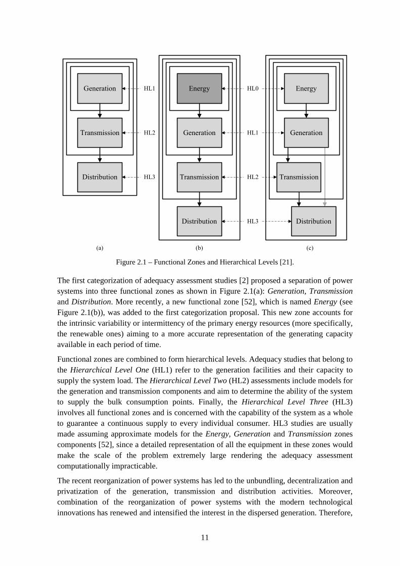
11

Figure 2.1 – Functional Zones and Hierarchical Levels [21].

The first categorization of adequacy assessment studies [2] proposed a separation of power systems into three functional zones as shown in Figure 2.1(a): Generation, Transmission and Distribution. More recently, a new functional zone [52], which is named Energy (see Figure 2.1(b)), was added to the first categorization proposal. This new zone accounts for the intrinsic variability or intermittency of the primary energy resources (more specifically, the renewable ones) aiming to a more accurate representation of the generating capacity available in each period of time.

Functional zones are combined to form hierarchical levels. Adequacy studies that belong to the Hierarchical Level One (HL1) refer to the generation facilities and their capacity to supply the system load. The Hierarchical Level Two (HL2) assessments include models for the generation and transmission components and aim to determine the ability of the system to supply the bulk consumption points. Finally, the Hierarchical Level Three (HL3) involves all functional zones and is concerned with the capability of the system as a whole to guarantee a continuous supply to every individual consumer. HL3 studies are usually made assuming approximate models for the Energy, Generation and Transmission zones components [52], since a detailed representation of all the equipment in these zones would make the scale of the problem extremely large rendering the adequacy assessment computationally impracticable.

The recent reorganization of power systems has led to the unbundling, decentralization and privatization of the generation, transmission and distribution activities. Moreover, combination of the reorganization of power systems with the modern technological innovations has renewed and intensified the interest in the dispersed generation. Therefore,

Generation

Transmission

Distribution

HL1

(a)

HL2

HL3

(b)

Generation

Transmission

Distribution

Energy HL0

HL1

HL2

HL3

Transmission

Distribution

Energy

(c)

Generation

12

a massive integration of this type of generating facilities into the distribution network has been promoted. According to these new developments, the traditional hierarchical level concept, which was developed under a centralized paradigm, was rendered obsolete and reformulated to include the generating capacity dispersed in the distribution network (see Figure 2.10(c)) [21].

The adequacy assessment studies and techniques described in this dissertation concern only the HL1 and HL2. HL2 studies are computationally more intensive than the ones of HL1. The evaluation of a HL2 system state, which includes one of the 8760 hourly load peaks as well as the availability of the primary energy resources, generating units and transmission circuits, requires power flow calculations rather than simple comparisons as, for example, the subtraction of the hourly system load from the total capacity available to detect loss of load in HL1 studies. Furthermore, remedial actions [5], like generation redispatch, are sometimes necessary in HL2 studies to eliminate potential violations of operating requirements, which makes the evaluation of HL2 states even more complex. A linear representation for the power flow equations is commonly adopted in HL2 studies to keep the computational effort at appropriate levels [5].

2.4. Generating Capacity Adequacy Assessment

The generating capacity adequacy assessment is an HL1 type of study [2]. Hence, only the Energy and Generation functional zones are considered. Hypothetically, it is assumed that all generating units and system loads are connected to a single bus. The generating capacity adequacy assessment studies can be divided according to the time span under analysis: the planning and operating phases.

Whenever the term generating capacity adequacy assessment is used in this dissertation, it refers to one specific planning study: the adequacy of the static reserve.

2.4.1. Planning Phase

The long-term adequacy assessment of the generating capacity can be viewed according to two different perspectives: static [2] and operating reserve [53], [54]. Static reserve studies aim to define the capacity necessary to meet the expected demand for a given level of risk. The uncertainty associated with the static reserve, which is a stochastic variable, is caused by the intermittency of the primary energy resources, the planned and forced outages of the generating units and the randomness of the system load.

The events of insufficient static reserve, RSTATIC, occur when the generating capacity is less than the load, according to

0<−= LGRSTATIC (2.1)

where G represents the generating capacity and L the system load.

13

On the other hand, the operating reserve studies are concerned with the long-term analysis of the flexibility of the generating system to cope with the short-term variations which can occur during the system operation [53], [54]. The generating capacity available in each operating period is affected by planned and forced outages and by the short-term fluctuations of the primary energy resources. Moreover, this capacity must be capable of not only supplying the load but also accommodating the difference between the short-term forecasts and the actual realizations of the stochastic variables while complying with the operational rules established by the utilities, such as, minimum primary and secondary reserve levels and unit commitment priorities. If the operational rules are available for different scenarios of operation, being a possible scenario the probabilistic combination of a wind and a hydrologic condition, it is possible to assess the adequacy of the operating reserve under a planning perspective.

Bearing these assumptions in mind, the identification of the events of insufficient operating reserve, ROPERATING, is made according to

GPLRRR WTSOPERATING ∆+∆+∆<+= (2.2)

where RS is the secondary reserve, RT is the tertiary reserve, ∆L and ∆PW are, respectively, the deviation of the realizations of the system load and wind power production from the respective short-term forecasts, and ∆G is the shortage of generating capacity due to forced outages during the operating period [53], [54]. A unit commitment of the available generating units must be made in order to calculate ROPERATING. The commitment of the units follows an iterative process according to predefined priorities. The priorities can vary depending on the availability of the primary energy resources, i.e., on the yearly scenarios of operation. This process stops when (2.3) is satisfied.

SPCOMMITTED RRLP ++≥ (2.3)

where PCOMMITTED is the committed generating capacity and RP is the primary reserve. RP and RS are deterministic variables and can take different values according to the scenario of operation. The variable RT is the total capacity available that was not committed and can be mobilized until the end of the operating period. It is assumed that mobilized units do not fail during starting-up. Finally, the value of the ROPERATING is

( )PTCOMMITTEDOPERATING RLRPR +−+= . (2.4)

Enhancements to the long-term adequacy assessment of the operating reserve have been recently proposed to include the mobility patterns of Electric Vehicles (EVs) and several charging strategies under different penetration scenarios [55], [56].

2.4.2. Operating Phase

The adequacy of the generating capacity in the operating phase is mainly concerned with the assessment of the unit commitment risk, i.e., which generating units should be used in the next operating period to guarantee that the probability of loss of load is below an

14

acceptable threshold [2], [57]. This threshold can be defined based on economic requirements or on decision-aid methods [57].

Historically, the adequate amount of operating reserve in the system has been set by utilities using deterministic criteria. For instance, some utilities establish that the operating reserve must be greater than or equal to the capacity of the largest committed unit [2]. Alternatively, the literature contains probabilistic methods that allow a more realistic assessment of the adequacy of the operating reserve. These methods aim to avoid overscheduling, which can be very costly, or underscheduling, which can compromise the continuity of supply. One of the most famous probabilistic methods is the PJM [2]. This method calculates the probability of loss of load given that no generating unit can be started during the operating period under evaluation. The effect of short-term load forecast uncertainty and derated or partial output states of the generating units can also be included [2].

Unfortunately, the first version of the PJM method does not include the possibility of modeling rapid start units during the operating period being assessed. These units must be modeled differently from those that have been committed since they can fail not only when they are properly synchronized but also during the starting-up process. Moreover, these models must account for the fact that the time required for the synchronization of these units depends on their status at the beginning of the operating period, i.e., if they are in hot or cold status. To overcome this limitation, a revised version of the PJM method was proposed [2].

Apart from the unit commitment risk assessment there is the operating problem of allocating, in an optimal way, the spinning reserve among the committed generating units so that the response risk to sudden changes during an pre-defined response time (e.g. load pick-up, wind power fluctuations or capacity decrease due to forced outages) is kept under a an acceptable threshold [2]. As a matter of fact, the effectiveness of the system to respond to these changes depends on the type of generating units used as spinning reserve. The assessment of the response risk includes the response rate of the units held as reserve, which is usually in MW/minute, and their failure probability during the required response time. The response risk can be also determined for different response times depending on the requirements defined for the deployment of the spinning reserve [2].

2.5. Composite Generation and Transmission Adequacy Assessment

The adequacy assessment of composite generation and transmission systems, or simply composite system, belongs to the HL2 type of studies [2], [5]. These studies include not only detailed models for the generating units and the system load but also for the transmission circuits. Therefore, the composite studies include more constraints than the generating capacity adequacy assessment studies, such as voltage limitations, maximum loading limits of the transmission circuits and real and reactive power considerations [2], [5]. Like in the case of HL1 studies, the adequacy of the composite system can be studied

15

considering a long-term or a short-term time span. All references to composite system adequacy assessment in this dissertation refer to the long-term analysis of the static conditions and not to operating reserve requirements.

2.5.1. Planning Phase

Clearly, the majority of composite system studies reported in the literature focus on determining the generating and transmission capacity necessary to provide a reliable supply to the bulk consumption [2], [5]. By including the transmission system, these studies are able to capture more accurately the effect of the geographic dispersion of the loads and primary energy resources on the long-term adequacy of the system. At present, there is no framework to include the transmission network in the long-term analysis of the adequacy of the operating reserve.

The adequacy of the composite system can be assessed for the system as a whole, for subsections of it, such as for the generation, transmission or the two subsystems altogether, and for each load bus [5]. A failure involving the generation subsystem is characterized by the inexistence of sufficient generating capacity to supply the system load: the amount of load curtailed corresponds exactly to the difference between the system load and the available generating capacity. A transmission subsystem failure occurs when there is load curtailment despite the fact that the generating capacity is sufficient to supply the system load. The remaining failures are attributed to the composite subsystem since they are caused by simultaneous deficit of the generating and transmission capacity.

Similarly to the generating capacity studies, the adequacy of a composite state depends on the ability of the system to supply the bulk consumption. As previously stated, the procedure used to detect loss of load is more complex than the simple comparison made by (2.1). In addition, different load curtailment priorities for the loads at the buses of the transmission network are commonly used to obtain a more accurate assessment of the continuity of supply of the bulk consumption [5].

2.5.2. Operating Phase

The literature has a limited number of composite studies [2], [58–61] that fit in the definition of operating phase presented in section 2.4.2. These studies refer only to the assessment of the unit commitment risk not to the response risk.

The first studies of unit commitment risk assessment considering the transmission system addressed possible bottlenecks between control areas due to shortage of tie line capacity [2]. Normally, these studies consider that the transmission system within each control area is completely reliable and with infinite capacity as well as different supporting philosophies between control areas.

16

To overcome the limitations of these first studies, several efforts have been made. The first approach that included a full representation of the transmission network was applied to the analysis of an academic power system containing 11 generating units, 8 transmission lines and a peak load of 185 MW [58]. Apart from other results, it has proved that common mode failure of transmission circuits and station initiated outages can contribute significantly to the unit commitment risk.

Differently from the approaches described in the last two paragraphs, some authors have tackled the HL2 unit commitment risk assessment by considering that it can be divided into two sub problems [59]. In first stage, unit commitment is performed to satisfy the normal operating criteria of HL1 studies. After that, an HL2 iterative analysis is made, committing one extra stand-by generating unit at a time, until the specified risk level is guaranteed.

2.6. Reliability Indices

The most important outcome of the probabilistic power system adequacy assessment studies is the reliability indices. In broad terms, reliability indices can refer to predictive and past performance indices [62]. Predictive indices provide information regarding the reliability of the system and are normally associated with the planning horizon. On the other hand, past performance indices reflect the actual system reliability and report the loss of load events observed. In this dissertation, only predictive indices are considered.

Traditionally, predictive reliability indices, from now on simply referred to as reliability indices, can have different designations depending on the hierarchical levels involved in the adequacy study. Despite the wide range of designations, reliability indices can be categorized as probability indices, energy indices and frequency and duration indices [2]. Examples of probability indices are [2]:

• Loss of Load Probability - LOLP, which gives the probability of load curtailment;

• Loss of Load Expectation - LOLE (hour/year, day/year or week/year), which represents the average number of hours, days or weeks during the evaluation period (usually a year) with load curtailment.

Examples of energy indices are [2]:

• Expected Power Not Supplied - EPNS (MW), which gives the average load curtailed;

• Expected Energy Not Supplied - EENS (MWh/year), which represents the average energy curtailed during the evaluation period (usually a year).

Examples of frequency and duration indices are [2]:

• Loss of Load Frequency - LOLF (occurrence/year), which represents the average number of load curtailment events during the evaluation period (usually a year);

• Loss of Load Duration - LOLD (hour/occurrence, day/occurrence or week/occurrence), which represents the average duration of a load curtailment event.

17

Only the aforementioned acronyms will be used in this dissertation to refer to probability, energy and frequency and duration indices.

Despite the valuable information the aforementioned indices convey, they cannot account for load curtailment cost. As a matter of fact, the overall load curtailment cost depends on the type of consumer disconnected (activities interrupted, electricity demand, the degree of dependency of its activity on electricity, etc.) and on the characteristics of the interruptions, such as the frequency, time of occurrence, curtailment depth and respective duration or even if the consumer was warned in advance [63], [64]. These individual costs are obtained from specific economic studies, like indirect analytical evaluation, analysis of actual blackouts or customer surveys. Surveys are preferably used since they are the most accurate way to determine the monetary losses that consumers have due to interruption on their supply.

The outcome of these studies is costumer damage functions, i.e., the average cost that each costumer class incurs after an interruption as a function of time [2]. If these damage functions are available for all costumer classes, then the reliability worth can be accurately measured through the following index [63], [64]:

• Loss of Load Cost - LOLC (currency/year), which represents the average cost of load curtailment during the evaluation period (usually a year).

Reliability indices are estimated by using test functions [5], which convert their definition into mathematical formulae. These test functions are used to check if system states are success or failure depending, respectively, if they are able to supply the system load or not. Reliability indices are the expected value of these test functions and have an underlying probability distribution [5].

2.7. The Well-being Analysis

As previously mentioned, the most important outcome of the probabilistic approach is the reliability indices. However, decision makers still pose some reluctance to the use of this information manly due to the difficulties in interpreting reliability indices. These difficulties can be overcome by incorporating deterministic criteria, such as the “N-1” criterion, in the probabilistic evaluation through the well-being concept [65], [66–68].

The well-being concept, which is depicted in Figure 2.2, can provide a measure of the degree for the success or failure of the system states by splitting them into Healthy, Marginal and At Risk. The Healthy states contain sufficient resources (generation and/or transmission) to meet the load and the pre-defined deterministic criteria. If the load can be supplied with the available resources but, at the same time, these resources are unable to comply with the pre-defined deterministic criteria, the state is deemed Marginal. Finally, if there are not enough resources to meet the system load, the state is deemed At Risk. Well-being indices are [67]:

• Probability of the Healthy State - P{H};

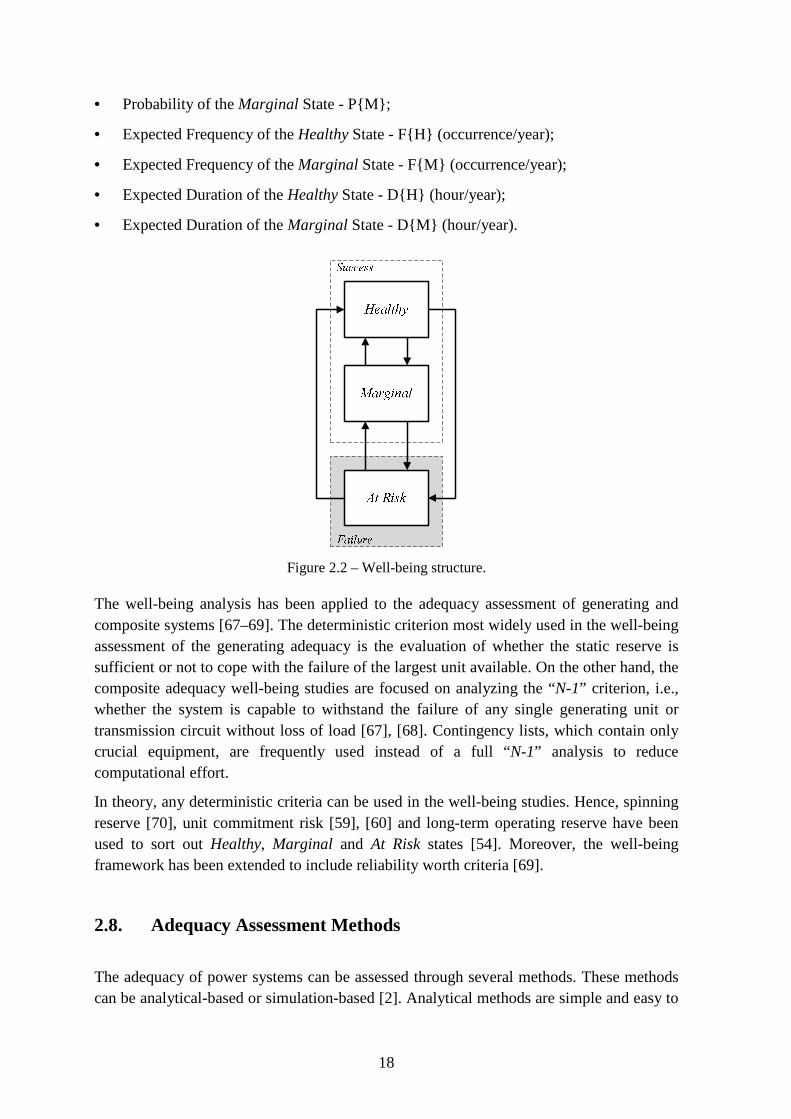
18

• Probability of the Marginal State - P{M};

• Expected Frequency of the Healthy State - F{H} (occurrence/year);

• Expected Frequency of the Marginal State - F{M} (occurrence/year);

• Expected Duration of the Healthy State - D{H} (hour/year);

• Expected Duration of the Marginal State - D{M} (hour/year).

Figure 2.2 – Well-being structure.

The well-being analysis has been applied to the adequacy assessment of generating and composite systems [67–69]. The deterministic criterion most widely used in the well-being assessment of the generating adequacy is the evaluation of whether the static reserve is sufficient or not to cope with the failure of the largest unit available. On the other hand, the composite adequacy well-being studies are focused on analyzing the “N-1” criterion, i.e., whether the system is capable to withstand the failure of any single generating unit or transmission circuit without loss of load [67], [68]. Contingency lists, which contain only crucial equipment, are frequently used instead of a full “ N-1” analysis to reduce computational effort.

In theory, any deterministic criteria can be used in the well-being studies. Hence, spinning reserve [70], unit commitment risk [59], [60] and long-term operating reserve have been used to sort out Healthy, Marginal and At Risk states [54]. Moreover, the well-being framework has been extended to include reliability worth criteria [69].

2.8. Adequacy Assessment Methods

The adequacy of power systems can be assessed through several methods. These methods can be analytical-based or simulation-based [2]. Analytical methods are simple and easy to

19

be used. They rely on mathematical analysis to calculate the exact value of the reliability indices or, at least, close enough approximations [2]. On the other hand, simulation methods provide estimates of the reliability indices bounded by an interval of confidence by simulating the stochastic behavior of the power system [5], [9], [10], [12], [71], [72]. The majority of adequacy assessment methods assume that the events in the system are independent. Even so, common mode failure events can also be modeled depending on the level of detail required [2].

2.8.1. Analytical-based Methods

Analytical methods rely on the enumeration of system states, or, more appropriately, they calculate the reliability indices by obtaining the probability mass function of the states. With this information available, the reliability indices are calculated according to

( )[ ] ( ) ( )xxXx

fHHEA∑ ∈

= (2.5)

where x is a realization of the random variable X, or, in other words, a system state, A is the set of all system states, f(x) is the probability of the system state x, H(x) is the outcome of the test function H for the system state x and E[H(X)] is a given reliability index mathematically represented by H. Note that a system state x is a vector that contains the states of the components of the system.

Analytical methods are divided into enumeration methods, approximate methods and PBMs. These methods can be didactic and computationally efficient. Nevertheless, they have two main drawbacks. Firstly, the complex behavior of the system can only be captured into simple mathematical models if assumptions are made. Secondly, some sort of space state pruning may have to be carried out since the number of system states increases exponentially with the number of components (for instance, the dimension of the state space for a system with N two-state components is 2N). As a result, the truthfulness of the reliability indices obtained with these methods can sometimes be questionable.

2.8.1.1. Enumeration Methods

Enumeration methods calculate the probability mass function of the system states, i.e., the probabilistic model of the states. This model is combined with the probabilistic load model to construct the system risk model. The reliability indices are calculated from the risk model. The distinctive feature between the different enumeration methods is the type of mathematical algorithm used to obtain the probabilistic model of the states. The first enumeration methods proposed were based on the conditional probability concept. These methods recursively add the probabilistic model of each component until all components are accounted for. The Loss of Load Expectation (LOLE) and the Frequency and Duration (F&D) [2] are well-known examples of methods which were developed specifically for the generating capacity adequacy assessment. While the LOLE method focus on obtaining the

20

probability of occurrence of all generating capacities on outage, the F&D method aims to calculate their underlying frequency of occurrence. Both methods are able to incorporate models for long-term load forecast uncertainty, scheduled maintenance, or even derated states of the generating units. Other methods, which are based on discrete convolution [73], are also available in the literature. These methods, which can use FFT [11], [74], are extremely fast when compared to the ones based on conditional probability especially in the case of very large generating systems. Frequency and duration indices can also be obtained using discrete convolution.

As for the case of the composite system adequacy assessment, there is considerable work on the methods based on conditional probability [2]. In this case, the probabilistic model of the system states is extended to include forced outages of transmission circuits. It is usually assumed that the number of simultaneously faulted transmission circuits is not greater than two (exceptions are allowed in case of common mode failures) to keep the computational effort within limits. To the knowledge of the author, discrete convolution techniques have not yet been applied to calculate the reliability indices for the composite system.

2.8.1.2. Approximate Methods

Some authors have proposed the use of continuous probabilistic expansions, like the Gram-Charlier [2], [75], [76] and Edgeworth [77], to approximate the probability mass function of the system states. These expansions are a function of the cumulants of the probability mass function of the system states. The calculation of the cumulants is done by recursively using the cumulants of the probability mass function of the components of the system. Usually, this calculation process is simple and computationally inexpensive.

The first approximate methods were proposed in the 1970s and 1980s. These methods were extensively applied to the generating capacity adequacy assessment of small and medium scale power systems. Despite their remarkable efficiency, it was observed that they can provide inaccurate reliability indices for the case of small scale systems [77]. The justification for this accuracy problem is twofold. Firstly, unless the number of random variables, in this case generating units, is sufficiently large, the expansion series are only appropriate for approximating continuous probability distributions. Secondly, there is no guarantee that the cumulative continuous probability distribution based on the Gram-Charlier or Edgeworth approximations is monotone [77]. With the development of fast and accurate algorithms for the discrete convolution of distributions, like the FFT, these approximate methods are falling into disuse. Even so, they have been applied recently to the probabilistic power flow problem [78].

2.8.1.3. Population-based Methods

Over the last decade there has been a considerable research effort on a new type of methods: the PBMs [32–34]. The core of these methods steam from optimization, more

21

specifically, from metaheuristics based on a population of solutions, like EA [35–37] or PSO [38]. These methods use the individuals of the population, which represent system states, to make a guided search through the state space in order to find the ones that contribute the most to the formation of the reliability indices. To keep the computational effort into acceptable levels, a truncation of the region of the space containing failure states is normally done (enumeration methods can also use truncation of the space).

The research on PBMs has reported remarkable computational efficiency, especially when the number of failure states is much smaller than the number of success states, or, in other words, when the cardinality of the subset containing the states that contribute to the formation of the reliability indices is small. Furthermore, the search efficacy, which measures error of the approximations of the reliability indices, and efficiency, which is related to the ratio of different states visited against the total number of states visited, can be enhanced by using spreading techniques [34].

PBMs have three main drawbacks. Firstly, since the estimates of the reliability indices are calculated using (2.5) no state should be saved twice in the memory. Thus a query to the memory must be made each time a new state is visited. For this reason, the memory must have sufficient capacity and fast in detecting whether new states have already been saved or not. Secondly, the stopping criterion of PBMs is gauged by the stability of the estimate of a given reliability index. After a number of iterations without meaningful alteration in the estimate of this index, it is assumed that the approximations of all indices are close to their accurate value and the search for new states is stopped. Due to the fact that a probability threshold is used to define a truncation of the state space, PBMs always underestimate the accurate value of the reliability indices. Thirdly and finally, it is not yet possible to evaluate the error of the estimates of the reliability indices.

2.8.2. Simulation-based Methods

Simulation methods are based on MCS [5], [10]. They can provide estimates of the reliability indices and an interval of confidence by simulating the stochastic behavior of power systems. The advantage of MCS over analytical methods is that the number of samples needed to guarantee a given level of accuracy for the estimates does not depend on the size of the power system but rather on its reliability [5]. Due to the flexibility of simulation methods, they have been extensively used in HL1 and HL2 studies.

Simulation-based methods can be classified according to how system states are sampled. If a state space representation is used, then the MCS method is called non-sequential. Conversely, when system states are sampled taking into account the chronology of events, the method is called sequential. Pseudo-sequential [71], pseudo-chronological [79] and quasi-sequential [80] MCS methods have also been proposed. These simulation-based methods do not adopt nor a pure state space nor a chronological representation.

The convergence of the MCS methods is monitored by the coefficient of variation β of the estimates of the reliability indices [10]. Considering H (H is normally a scalar function) as

22

a test function representing a given reliability index, the coefficient of variation is calculated according to

( )[ ][ ]( )[ ]X

X

HE

NHEV~=β (2.6)

where N is the number of samples, ( )[ ]XHE~

is the estimate of a given reliability index

represented mathematically by H and ( )[ ][ ]XHEV is the variance of the distribution of the

reliability index. This variance can be estimated using the unbiased estimator

( )[ ][ ] ( ) ( )[ ]( )∑=

−−

=N

i

i HEHN

HEV1

~

1

1~XxX (2.7)

where xi is one system state over the N sampled [10]. The suitable test function for each reliability index depends on the MCS method [5].

Figure 2.3 – State space representation.

Assume now that the parameter to be estimated by a simulation-based method is µ = E[H(X)]. The Central Limit Theorem (CLT) [81] states that the sum of independent and identically distributed (iid) variables

( )

−

= ∑=

µσ

N

i

iHN

Z1

x (2.8)

tends to the Gaussian distribution with zero mean and variance 1 as N → ∞. For any z ≥ 0, it is possible to find the numbers –z and z between which Z lies with probability 1 – α. Mathematically, this is equivalent to

( ) α−=≤≤− 1zZzP . (2.9)

The number z can be obtained via the cumulative probability distribution as

( ) ( )21Φ21)(Φ 1 αα −=⇒−=≤= −zzZPz . (2.10)

Given the probability 1 – α, the interval of confidence for µ is

23

( ) ( ) ασαµµσαµ −=

−+≤≤−− −− 121Φ~21Φ~ 11

NNP . (2.11)

Normally, the interval of confidence can be rewritten as function of the coefficient of

variation. Finally, by knowing that µ = E[H(X)] and that the coefficient of variation of µ~

is given by (2.6), the equation for the interval of confidence for µ is

( )[ ] ( )[ ]( ) ααβµµαβµ −=−×−×≤≤−×−× −− 121Φ1~21Φ1~ 11P . (2.12)

For instance, for a typical β = 0.05 and 1 – α = 0.95, the interval of confidence is:

( ) 95.0098.1~902.0~ =×≤≤× µµµP . (2.13)

2.8.2.1. Non-sequential Monte Carlo Simulation Method

In non-sequential MCS, system states are sampled by taking “snapshots” of its stochastic behavior, i.e., the state of all components is sampled without considering any time-dependency between consecutive states. The reliability indices are estimated by “statistically scanning” the state space, which is symbolically illustrated in Figure 2.3. Mathematically, this is written as

( )[ ] ( )i

N

i

HN

HE xX ∑=

=1

1~ (2.14)

where xi is a sampled system state, N is the number of samples, H(xi) is the outcome of the

test function H for the system state xi and [ ])(~

XHE is the estimate of a given reliability

index represented mathematically by H. As an example, a possible test function [82] for the LOLP index is

( )Xsi

Xfii

S

S

if

ifH

∈∈

=

x

xx

0

1LOLP (2.15)

where XfXsX SSS U= is the set of all system states divided into the subsets of success

states, SXs, and failure states, SXf,.

The test function [82] for the EPNS index is

( )Xsi

Xfiii

S

S

if

ifPH

∈∈

∆

=x

xx

0EPNS (2.16)

where ∆Pi is the loss of load of the state xi.

Frequency and duration calculations following a state space representation can be a complex task [82]. The traditional way of making these calculations involves enumerating all success states which can be reached from a failure one, or, all the failure states which can be reached from a success one by changing the state of only one components of the system [82]. This enumeration process is preferably used in generating capacity studies

24

where the computational effort of enumerating and evaluating states is reduced. According to this definition, the following test function [82] can be used for the LOLF index:

( )Xsi

Xfikik

ik

iS

S

if

ifH

∈∈

=∑

≠x

xx

0,LOLF

λ (2.17)

where λik is the transition rate between the failure state xi and the success state xj that can be reached from xi by changing the state of only one component of the system.

In the case of composite studies, where the computational effort required for the same enumeration task is considerably higher, the one-step forward state transition technique [68] is preferable since it only requires the composition and evaluation of one extra state in addition to sampled failure one. Non-sequential MCS cannot easily include chronological aspects of the system operation, such load, hydrologic or wind variation. Even so, efforts have been made to circumvent this limitation [16], [83]. Since non-sequential MCS is based on the state space representation, it is not possible to model non-Markovian processes [5].

2.8.2.2. Sequential Monte Carlo Simulation Method

The sequential MCS method samples system states by “setting in motion” a virtual or fictitious clock and, with the flow of time, sequences of events are synthetically generated creating the “life story” power system. The sequential MCS method guarantees that two consecutive system states differ from one another in the state of only one component [5], [9]. Since this approach can sequentially reproduce the operation of the system, it is easy to include all chronological aspects such as time and spatially correlated load models, the capacity fluctuation of renewable power sources, the customer damage functions per area or bus, programmed maintenance schedules, etc. Moreover, non-Markovian models for representing failures of components can be adopted and the probability distributions of the adequacy indices can be obtained [5], [9].

Figure 2.4 – Simplified representation of a sequence of events over a period of time T.

...

G (MW)

L (MW)

1 2 3 4 5 6 7 8 9 10 T0

25

As a simple example, Figure 2.4 depicts how system states are sampled by the sequential MCS method for the generating capacity adequacy assessment. The shaded areas in this figure represent the energy curtailed due to capacity outages. This figure also demonstrates that the state transition between different load levels is made in fixed time steps whereas the duration of the states of the generating units is not fixed (it depends on the underlying probability distribution).

Like the sequential MCS method, the estimation of the reliability indices is according to

( )[ ] { }( )∑

===

NY

i

Snn

iHNY

HE1

1

1~xX (2.18)

where { } { }SiSnn

i xxx ,...,11 == , Si ∈ ℕ, is the synthetic sequence of system states x over the

period i and NY is the number of periods simulated. As an example, the test function H of the index LOLP, which is evaluated at the end of each simulated period T, can be defined as

{ }( ) ( ) ( )n

S

n

nSnn Hd

TH

ii xxx LOLP

11LOLP

1 ×= ∑=

= . (2.19)

where xn is the n-th state of the sequence, T is the duration of the synthetically simulated period (typically T = 8760 h), d(xn) is the duration of the state xn and HLOLP(xn) is the outcome of (2.15) taking xn as argument.

The following test function can be used for case of the EPNS index

{ }( ) ( ) ( )n

S

n

nSnn Hd

TH

ii xxx EENS

11EENS

1 ×= ∑=

= . (2.20)

where HLOLP(xn) is the outcome of (2.16) taking xn as argument.

Unlike non-sequential MCS, frequency and duration calculations are very easy to do: the detection of load curtailment events is made only by “following” the sequential simulation of the system as

{ }( ) ( )∑=

−= =i

i

S

n

nnSnn hH

211LOLF ,xxx . (2.21)

where

( )otherwise

SandS

if

ifh

XsnXfnnn

∈∈

= −

−1

10

1,

xxxx . (2.22)

2.8.2.3. Variants of Monte Carlo Simulation

Several variants of the non-sequential and sequential MCS methods are available in the literature. Their purpose is to reduce the computational effort while retaining the flexibility and accuracy of the sequential MCS method. Among others, the most important ones are

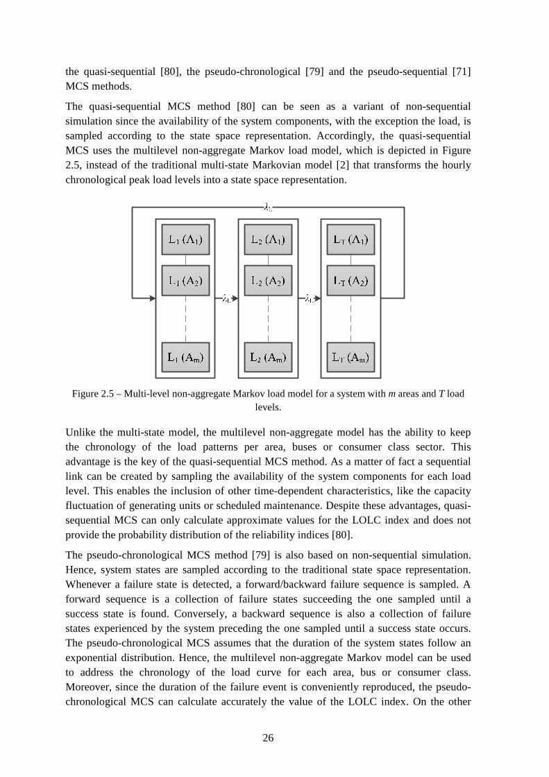
26

the quasi-sequential [80], the pseudo-chronological [79] and the pseudo-sequential [71] MCS methods.

The quasi-sequential MCS method [80] can be seen as a variant of non-sequential simulation since the availability of the system components, with the exception the load, is sampled according to the state space representation. Accordingly, the quasi-sequential MCS uses the multilevel non-aggregate Markov load model, which is depicted in Figure 2.5, instead of the traditional multi-state Markovian model [2] that transforms the hourly chronological peak load levels into a state space representation.

Figure 2.5 – Multi-level non-aggregate Markov load model for a system with m areas and T load levels.

Unlike the multi-state model, the multilevel non-aggregate model has the ability to keep the chronology of the load patterns per area, buses or consumer class sector. This advantage is the key of the quasi-sequential MCS method. As a matter of fact a sequential link can be created by sampling the availability of the system components for each load level. This enables the inclusion of other time-dependent characteristics, like the capacity fluctuation of generating units or scheduled maintenance. Despite these advantages, quasi-sequential MCS can only calculate approximate values for the LOLC index and does not provide the probability distribution of the reliability indices [80].

The pseudo-chronological MCS method [79] is also based on non-sequential simulation. Hence, system states are sampled according to the traditional state space representation. Whenever a failure state is detected, a forward/backward failure sequence is sampled. A forward sequence is a collection of failure states succeeding the one sampled until a success state is found. Conversely, a backward sequence is also a collection of failure states experienced by the system preceding the one sampled until a success state occurs. The pseudo-chronological MCS assumes that the duration of the system states follow an exponential distribution. Hence, the multilevel non-aggregate Markov model can be used to address the chronology of the load curve for each area, bus or consumer class. Moreover, since the duration of the failure event is conveniently reproduced, the pseudo-chronological MCS can calculate accurately the value of the LOLC index. On the other

27

hand, scheduled maintenance can be only approximately included in pseudo-chronological simulation and, like the quasi-sequential approach, the probability distribution of the reliability indices cannot be obtained.

Contrasting with the quasi-sequential and pseudo-chronological, the pseudo-sequential MCS method [71] is based on the sequential MCS method. It is based on the observation that the computational effort required to create synthetic yearly sequences of states is negligible when compared with the effort of composing and evaluating these states. Moreover, since most of the states within a synthetic sequence do not contribute to the reliability indices, additional savings in computational effort can be made if only failure states undergo the process of evaluation. Taking the aforementioned into account, the first procedure of pseudo-sequential MCS method is to sample several yearly synthetic sequences of states using the same procedure as the sequential MCS method. Subsequently, a state space sampling process is made to sample, firstly, one of the various synthetic sequences and, secondly, one hour of the year. If the state sampled is failure, the forward/backward sequences of failure states are composed and evaluated until these sequences are bounded by success states. If the state is success, then the two-step state space sampling process is repeated until a new failure state is found. The pseudo-sequential MCS method retains all the modeling advantages of the sequential MCS method and is able to provide accurate estimates of the LOLC index. However, like all the former simulation-based variants, the probability distribution of the reliability indices cannot be obtained. The main shortcoming of the pseudo-sequential MCS method is to know when a suitable number of synthetic sequences have been sampled to ensure that the estimates the reliability indices are unbiased.

2.9. The Sequential MCS Method for the Adequacy Assessment of Power Systems

The sequential MCS method developed in this dissertation includes models for the availability of the generating units, for the hydro and wind capacity fluctuation and for the chronology of the load. Since two different adequacy problems are used in this dissertation, namely the adequacy of the generating capacity and the composite system, the method must be able to evaluate these two different long-term problems satisfactorily. For that reason, the sequential MCS method developed contains models for forced outages of the transmission lines and transformers and for the power flow analysis. The next sections describe in detail all the models used.

2.9.1. Models of the System Components

The capacity of the components of the system depends on two distinct models:

• The failure/repair cycle stochastic model;

28

• The capacity time-dependent model.

The first model is related to the stochastic behavior of forced outages. It defines the availability of the component, i.e., the transitions between the up and down states. The availability of a component can be seen as the maximum capacity that it has when in a given state. The failure/repair cycle stochastic models considered in this dissertation are the two-state and the multistate Markov models [9], [10].

Figure 2.6 – Two-state Markov model (λ is the failure rate and µ is the repair rate).

A component, whose failure/repair cycle stochastic model is the two-state Markov model (see Figure 2.6), has its maximum capacity available when in the up state. In the down state, the capacity is zero. Assuming that the states duration are exponentially distributed, the residence time in the up and down states is given by the inverse transform method [10] according to

1ln1

UTUp

λ−= (2.23)

2ln1

UT Down

µ−= (2.24)

where TUp is the residence time in the up state, TDown is the residence in the down state, U1 e U2 are uniformly distributed numbers sampled from the interval [0,1].

Figure 2.7 – Multistate Markov model (λ is the failure rate, µ is the repair rate, N is the number of components of the aggregation, Ck is a state which contains N-k components in the up state).

If the failure/repair cycle of an aggregation of N components is iid, one can use the multistate Markov model (see Figure 2.7). In this case, the maximum capacity of the state Ck is

( ) CkNCk

×−=C (2.25)

where N is the number of iid components, k = 0, 1, …, N and C is the capacity of one component. If the duration of the states is exponentially distributed, the residence time in the states C0 and CN is

29

1ln1

0 UN

Tλ

−=C (2.26)

( ) 2ln1

1U

kT N

µ+−=C (2.27)

where 0CT is the residence time in the state C0, NTC is the residence time in CN, and λ and µ are respectively the failure and repair rates of one component of the aggregation. As for the remaining states, the residence time is calculated via

( )

−

−−= 21 ln

1,ln

1min U

kU

kNT k

µλC . (2.28)

It is common to use the parameters Mean Time to Failure, MTTF, and Mean Time to Repair, MTTR, instead of λ and µ. These parameters can be obtained using [2]

λ1=MTTF (2.29)

µ1=MTTR . (2.30)

On the other hand, the second model is concerned with the representation of the time dependence of the capacity of the components. This is of the utmost importance since the capacity of some components exhibits an hourly, monthly or even yearly variation [53], [54]. This time-dependent characteristic is captured by hourly/monthly series with probabilities associated. These series are obtained for several years of observations.

2.9.1.1. Conventional Generating Units

Conventional generating units are the ones that convert the thermal energy contained in fossil fuels or in the atomic nucleus to electricity via a thermodynamic cycle. The failure/repair cycle of this type of generating units is represented by a two-state Markov model and its transitions follow an exponential probability distribution.

When in the up state, a conventional generating unit is able to produce its maximum capacity. Conversely, the capacity is zero when in the down state.

2.9.1.2. Hydro Generating Units

Hydro generating units are the ones that convert the potential energy of the water to electricity. Like conventional generating units, the failure/repair cycle is also represented by a two-state Markov model with transitions that follow an exponential probability distribution.

The capacity time-dependent model of the hydro units is complex since the power output depends on the levels of water stored in the reservoirs and on the inflows. As a simple but

30

robust approach, it is common to use several hydrological series, which are based on the historical observations and have probabilities associated, that capture a proportional relationship between the total water stored in the reservoir and the power produced by the corresponding hydro generating unit in each month of the year [53], [54]. The use of this simple model is justified due to the high complexity related to establishing dispatch conditions for the long-term [54]. The capacity available in each month is calculated by multiplying the maximum capacity, which is obtained from the failure/repair stochastic model, with the corresponding monthly value of the hydrological series. These series are constructed based on records collected over several years. Despite the probabilistic nature of the hydrological series, they are a deterministic input of the sequential MCS method. When a new synthetically generated year begins, a hydrological year is sampled and each hydro unit is assigned its corresponding hydrological series. All the same, more detailed models, which are based on the volumes of water stored in the reservoirs, can also be used, especially if pumping schemes are considered [53].

2.9.1.3. Wind Farms

WTGs are all those that convert wind energy to electricity. Taking advantage of the fact that WTGs within WFs traditionally are equal, the multistate Markov model is used to represent the failure/repair cycle of the whole WF. In this model, the transitions between states follow an exponential probability distribution. Similarly to the capacity time-dependent model of hydro units, the maximum capacity of the states is multiplied by the corresponding value taken from hourly wind series. These series capture the hourly production of the WFs in percentage of their total capacity. Despite having a probabilistic nature, they are used as input parameters of the sequential MCS method, in the same way as the hydrological series. An advantage of using the sequential MCS method is that there is no need to build models for spatial and time correlations for WFs at different sites since these correlations are implicitly enclosed in the historical series and are naturally accounted for as the simulation sequentially advances through time.

2.9.1.4. Transmission Lines and Transformers

The failure/repair cycle for transmission lines and transformers is modeled by a two state Markov model, with transitions that follow an exponential distribution. It is assumed that the maximum capacity remains unchanged over time.

2.9.1.5. Load

The load is modeled using a chronological representation that contains a load level for each hour of the year. The sequential MCS method follows chronologically these loads steps as

31

the simulation progresses. In addition, each load bus has its own hourly load profile in percentage of its peak load. Each hourly load percentage is obtained by dividing the peak load of that hour by the peak load of the year.

Short-term and long-term load forecast uncertainties can also be included in the simulation [2]. There are methods based on the continuous Gaussian [81] distribution and on discrete representations of it.

Due to the flexibility of the sequential MCS method, there is no need of using discrete representations of the Gaussian distribution. The inclusion of the short-term uncertainty on the sequential simulation consists of adding to the hourly load value a random number sampled from the continuous Gaussian distribution with a zero mean and a standard deviation, σST. Likewise, the long-term uncertainty is accounted for by adding the annual peak load a random number sampled from the continuous Gaussian distribution with a zero mean and a standard deviation, σLT. Both standard deviations, which control the amplitude of the uncertainty, are pre-specified at the beginning of the simulation.

2.9.2. Simulation Algorithm

The algorithm of the sequential MCS method for the generating capacity and the composite system adequacy assessment is based on the following general steps:

Step a) Define the maximum number of years to be simulated, NMAX, the tolerance for the relative uncertainty (β), set the simulation time, h, to 0 and set the number of years simulated, NYEAR, to 1

Step b) Update the simulation time: h: = h + 1

Step c) Select a system state (select the availability of the components according to their stochastic failure/repair cycle model and the capacity time-dependent model, select the load level, etc.)

Step d) Evaluate the system state selected (compose the state and check if the load level can be supplied with the available generating and/or transmission capacity without violating operating limits; If not, apply remedial actions, such as generation redispatch and/or load curtailment)

Step e) Update the outcome of the test functions of the reliability and other indices

Step f) If h = 8760, store the reliability indices, update their relative uncertainty (β), and advance to Step g); If not, go back to Step b)

Step g) If NYEAR is equal to NMAX or if the relative uncertainties of the reliability indices are less than the specified tolerance, stop the simulation; otherwise, NYEAR := NYEAR + 1, h = 0, and go back to Step b)

The reliability indices normally used to gauge the convergence of the simulation process are the ones associated to the overall performance of the system and not the ones of the individual bulk consumption points. At the end of the simulation process, the sequential

32

MCS method can provide not only estimates of the reliability indices but also their underlying probability mass function.

The Step d) of the sequential MCS method is concerned with the state evaluation. This is the most complex part of the method since it encloses different procedures depending whether the generating capacity or the composite system adequacy is being assessed. The following sections outline the procedures necessary to perform both evaluations.

2.9.2.1. Generating Capacity Evaluation

The procedure used to evaluate the adequacy of the generating capacity is quite straightforward: if the generating capacity is sufficient to supply the load, then there is no load curtailment and the state is deemed as success. On the contrary, the total load loss is calculated and the state is deemed as failure.

2.9.2.2. Composite System Evaluation

In composite system adequacy studies, transmission components are subjected to failures. Therefore, the first procedure consists of determining the connectivity between buses. Subsequently, a dispatch procedure is made to distribute the load to the available generating units. After that, the state of the transmission system is assessed by running a Power Flow (PF) [84]. If there are circuits with operating limits violated, then an Optimal Power Flow (OPF) [85] is executed to apply remedial actions and determine the minimum load curtailment or minimum loss of load cost. As there are several procedures in the evaluation of a composite state, it is important that they are executed rapidly and, most of all, in a reliable way, since any misevaluated state due to, for instance, numerical failures, might affect considerably the accuracy of the estimates of the reliability indices, especially in the case of very reliable power systems.

2.9.2.2.1. Transmission Network Configuration

The transmission network configuration procedure is based on a list search method. This method assumes that the network is described by a node/branch representation, i.e., a node is a bus and a branch is a transmission circuit. All nodes are numbered and each branch connects two different nodes. The main objective is to identify the electric islands and the nodes/branches they enclose. The algorithm [86] is as follows:

Step a) Initialize a vector v, which is named vector of indicators, by assigning each entry i an indicator, according to vi = i

Step b) Create a temporary vector, vT = v and browse the list of branches until all branches are checked

33

If the branch connecting node i to j is in the up state, then vi and vj are updated according to

{ }jiji vvvv ,min== . (2.31)

If the branch connecting node i to j is in the down state, then go to the next branch

Step c) If v ≠ vT, then go to Step b); If not, continue to Step d)

Step d) Assign each node an electric island: the nodes belonging to the same electric island have the same indicator; The number of different electric islands is equal to the number of different indicators in v

2.9.2.2.2. Generating Units Dispatch

This procedure consists of allocating the hourly load to the available generating units taking into account their restrictions. It can follow a merit order or a proportional strategy. The merit order strategy is according to the following steps:

Step a) Find the next available generating unit with the highest merit that has not been dispatched yet

Step b) Dispatch the generating unit with its full capacity or with the remaining load, whichever is lower

Step c) If all load has been allocated end the procedure; Otherwise go to Step a)

In the proportional strategy, the power dispatched to each generating unit is proportional to its capacity and the total available generating capacity, according to

( )i

NG

jjNG

jjj

ii

i PPL

PP

PPP +

−×

−

−= ∑∑ =

=

1

1

(2.32)

where Pi the production of the generating unit i, iP is its maximum capacity, iP is the its

minimum capacity, NG is the number of generating units available and L is the load.

2.9.2.2.3. DC Power Flow

The DC PF task consists of checking if there are transmission lines or transformers operating outside their loading limits. A linearized representation of the power flow equations is adopted so that direct mathematical methods can be used instead of numerical methods, which reduces the computational effort considerably.

The quality of the linearization depends on the characteristics of the power system, namely on the voltage level and on the type of transmission lines. The error made by using the

34

linearized representation decrease with the increase of the voltage level and the number of overhead transmission lines. This representation cannot analyze the impact of reactive power and bus voltages on the adequacy of the system. This simplification is tolerable if a long-term analysis is being made.

The DC PF [84] consists of solving the following system of linear equations

θBPP '=− LG (2.33)

where PG and PL are, respectively, the vectors of real power produced and consumed at each bus, B' is the susceptance matrix of the DC representation and θ is the vector of bus voltage angles.

The entries of the susceptance matrix are calculated according to

kix

Bik

ik ≠∀−= ,1

' (2.34)

kix

BNB

kii ikii =∀−= ∑

≠=

,1

',1

(2.35)

where NB is the number of buses and xik the reactance of the branch connecting bus i to k.

The system of linear equations represented by (2.33) is undetermined. By zeroing the bus voltage angle of one bus, one can eliminate one equation resulting in

θBPP ˆ'ˆˆˆ =− LG . (2.36)

The real power flow through the branch connecting bus i to k is

ik

kiik

xP

θθ −= . (2.37)

Combining (2.36) with (2.37), the DC sensitivity matrix A is obtained. This matrix relates the loading of the branches with the real power injected at the buses according to

( )LGik PPAP ˆˆ −= . (2.38)

2.9.2.2.4. DC Optimal Power Flow

If, at the end of the DC PF task there are transmission lines and transformers operating outside their loading limits, a DC OPF [85] is run. This task consists of enforcing the operating limits of the system components by altering the real power injected at the buses. The objective is to minimize the total load curtailed, if there is the need of such corrective measure. In mathematical form, the DC OPF is

min. ∑=i

GFii PMz (2.39a)

s. t. LGF PP0 ≤≤ (2.39b)

35

GGG PPP ≤≤ (2.39c)

ikik PΓZθP ≤≤ (2.39d)

0θBPPP =+−+ 'LGFG (2.39e)

where PGF is the vector of real power produced by the fictitious generating units that model the load curtailment, Mi is a constant that reflects the load curtailment priority of the load at bus i, PG is the vector of the real power produced by the generating units, PL is the vector of real power consumption, Г is a diagonal matrix whose entries are the inverse of the branches reactance, Z is the branch-bus incidence matrix, θ is the vector of bus voltage angles and the B' is the susceptance matrix of the DC PF. Other objective functions [5], such the minimization of the load curtailment cost, can also be used.

Two different approaches are available in the literature to solve (2.39): the Simplex method [87] and the Interior Point or Barrier methods [88]. The method selected for the DC OPF task was the Simplex method. A free software package, which is named LPSolve® [89] and is under the GNU lesser general public license, was included in the sequential MCS method. This software is based on the Revised Simplex method [90].

2.9.3. Validation of the Sequential Monte Carlo Simulation Method

The accuracy of the sequential MCS method was tested by assessing the adequacy of the generating capacity and the composite system of several test systems. The objective of these experiments was to determine how close the estimates of the reliability indices are from the results published in the literature.

Three test systems were used to validate the accuracy of the sequential MCS method for the generating capacity: the small-sized IEEE-RTS 79 [91] and the medium-sized IEEE-RTS 96 [92] and IEEE-RTS 96 HW [54] systems. The IEEE-RTS 96 HW is a variant of the IEEE-RTS 96 that includes the time-dependency of hydrological and wind resources. The accuracy of the sequential MCS method for the composite system adequacy assessment was tested by using the IEEE-RTS 79 [91], the IEEE-MRTS 79 [93] and the IEEE-MRTS 96 [93] systems. The MRTS variants differ from the original configurations of the IEEE-RTS 79 and IEEE-RTS 96 systems in the capacity of the generating units and the annual peak load: these deterministic parameters are multiplied by a factor of two in order to stress the transmission system.

2.9.3.1. Test Systems

The IEEE-RTS 79 was developed to fulfill the need for a standardized database to test and compare results between different adequacy assessment methods. This test system is composed of 24 buses, 32 generating units, 33 transmission lines and 5 transformers. The

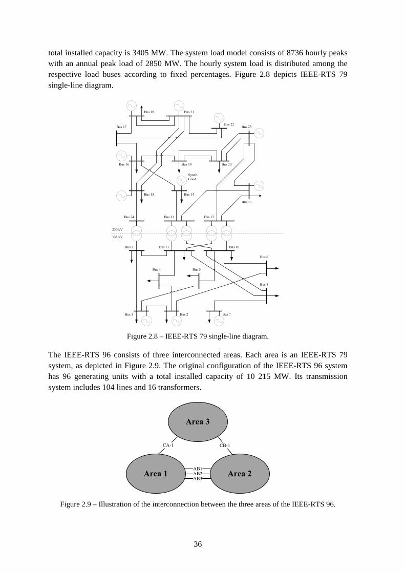
36

total installed capacity is 3405 MW. The system load model consists of 8736 hourly peaks with an annual peak load of 2850 MW. The hourly system load is distributed among the respective load buses according to fixed percentages. Figure 2.8 depicts IEEE-RTS 79 single-line diagram.

Figure 2.8 – IEEE-RTS 79 single-line diagram.

The IEEE-RTS 96 consists of three interconnected areas. Each area is an IEEE-RTS 79 system, as depicted in Figure 2.9. The original configuration of the IEEE-RTS 96 system has 96 generating units with a total installed capacity of 10 215 MW. Its transmission system includes 104 lines and 16 transformers.

Figure 2.9 – Illustration of the interconnection between the three areas of the IEEE-RTS 96.

Bus 1 Bus 2

Bus 3

Bus 7

Bus 5Bus 4

Bus 6

Bus 8

Bus 10Bus 11

Synch.

Cond.

Bus 15

Bus 24 Bus 11 Bus 12

Bus 14

Bus 13

Bus 20Bus 19Bus 16

Bus 17

Bus 18 Bus 21

Bus 22Bus 23

230 kV

138 kV

Area 1

Area 3

Area 2

CA-1

AB2AB1

AB3

CB-1

37

The annual peak load of this system is 8550 MW. The load model is represented by 8736 hourly peaks. Like the case of the IEEE-RTS 79, the system load is distributed by the load buses according to fixed percentages. Three transmission lines make the interconnection between Area 1 and Area 2: AB1 connects bus 107 with bus 203; AB2 connects bus 113 with bus 215; AB2 connects bus 123 with bus 217. Area 3 is connected to Area 2 through the line CB-1, which links bus 318 with bus 223. Lastly, the transmission line CA-1 interconnects buses 325 and 121. The two terminal DC transmission lines between bus 113 and bus 316 have not been considered.

Table 2.1 – Generating capacity reliability indices for the IEEE-RTS 79.

IEEE-RTS 79 LOLE (h/yr) EENS (MWh/yr) LOLF (occ./yr) Analytical [11] 9.394 1176.30 2.025

Sequential MCS 9.370 1163.00 2.024 β (%) 0.70 1.00 0.56

99% Interval of Confidence [9.201, 9.538] [1132.99, 1193.00] [1.994, 2.053]

The IEEE-MRTS 96 installed capacity and annual peak load are 20 430 MW and 17 100 MW, respectively. All other parameters are identical to those of the IEEE-RTS 96 system.

The IEEE-RTS 96 HW is obtained from the IEEE-RTS 96 by replacing the 350 MW unit of the Area 1 by 1526 MW of wind capacity. With this modification, the renewable share increases from 8.8% to 21.3%. The wind capacity is composed by 763 wind turbine generators (WTGs) of 2 MW (MTTF = 1914.74 h and MTTR = 80 h). These units are distributed over the three areas. WF1 has 267 units and is located in Area 1. WF2 has 229 and is in Area 2. WF3 is composed of 267 units and belongs to Area 3.

The wind capacity fluctuation in each of the three areas is characterized by three series. They are labeled as favorable, average and unfavorable. Their probabilities of occurrence are 25%, 50% and 25%, correspondingly. These series can be obtained from [54]. The capacity fluctuation of each cluster of six hydro units is characterized by five hydro series. These series have the same probability of occurrence and can be obtained from [54]. The hourly load model of the IEEE-RTS 96 HW includes the 28th day of February by copying the twenty-four hourly peaks of the previous day.

2.9.3.2. Generating Capacity Results

Table 2.1 shows the estimates of the reliability indices of the generating capacity of the IEEE-RTS 79 obtained with the sequential MCS method. The coefficient of variation of the estimates of the LOLE, EENS and LOLF at the end of the simulation is also reported in this table.

The simulation was stopped when all estimates had a coefficient of variation less than or equal to 1%. The intervals of confidence were calculated for a 99% probability level.

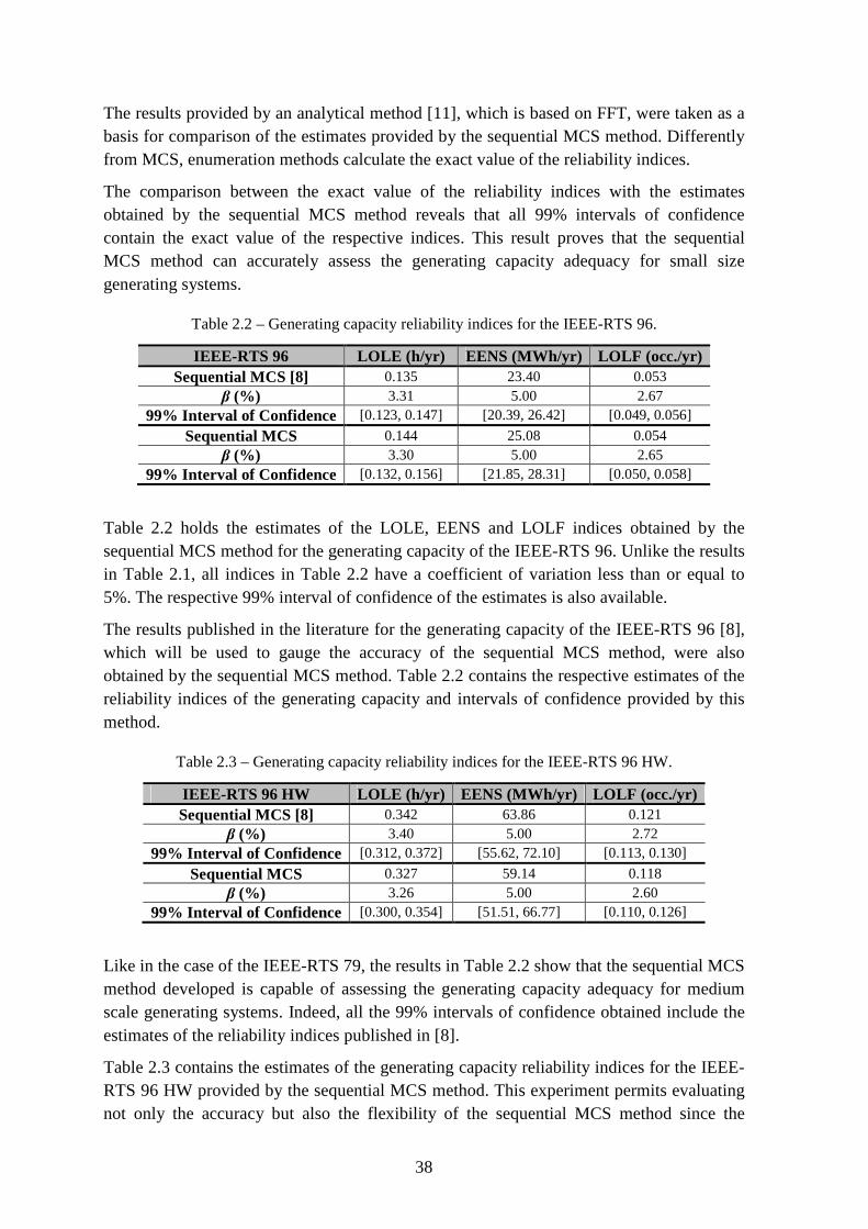
38

The results provided by an analytical method [11], which is based on FFT, were taken as a basis for comparison of the estimates provided by the sequential MCS method. Differently from MCS, enumeration methods calculate the exact value of the reliability indices.

The comparison between the exact value of the reliability indices with the estimates obtained by the sequential MCS method reveals that all 99% intervals of confidence contain the exact value of the respective indices. This result proves that the sequential MCS method can accurately assess the generating capacity adequacy for small size generating systems.

Table 2.2 – Generating capacity reliability indices for the IEEE-RTS 96.

IEEE-RTS 96 LOLE (h/yr) EENS (MWh/yr) LOLF (occ./yr) Sequential MCS [8] 0.135 23.40 0.053

β (%) 3.31 5.00 2.67 99% Interval of Confidence [0.123, 0.147] [20.39, 26.42] [0.049, 0.056]

Sequential MCS 0.144 25.08 0.054 β (%) 3.30 5.00 2.65

99% Interval of Confidence [0.132, 0.156] [21.85, 28.31] [0.050, 0.058]

Table 2.2 holds the estimates of the LOLE, EENS and LOLF indices obtained by the sequential MCS method for the generating capacity of the IEEE-RTS 96. Unlike the results in Table 2.1, all indices in Table 2.2 have a coefficient of variation less than or equal to 5%. The respective 99% interval of confidence of the estimates is also available.

The results published in the literature for the generating capacity of the IEEE-RTS 96 [8], which will be used to gauge the accuracy of the sequential MCS method, were also obtained by the sequential MCS method. Table 2.2 contains the respective estimates of the reliability indices of the generating capacity and intervals of confidence provided by this method.

Table 2.3 – Generating capacity reliability indices for the IEEE-RTS 96 HW.

IEEE-RTS 96 HW LOLE (h/yr) EENS (MWh/yr) LOLF (occ./yr) Sequential MCS [8] 0.342 63.86 0.121

β (%) 3.40 5.00 2.72 99% Interval of Confidence [0.312, 0.372] [55.62, 72.10] [0.113, 0.130]

Sequential MCS 0.327 59.14 0.118 β (%) 3.26 5.00 2.60

99% Interval of Confidence [0.300, 0.354] [51.51, 66.77] [0.110, 0.126]

Like in the case of the IEEE-RTS 79, the results in Table 2.2 show that the sequential MCS method developed is capable of assessing the generating capacity adequacy for medium scale generating systems. Indeed, all the 99% intervals of confidence obtained include the estimates of the reliability indices published in [8].

Table 2.3 contains the estimates of the generating capacity reliability indices for the IEEE-RTS 96 HW provided by the sequential MCS method. This experiment permits evaluating not only the accuracy but also the flexibility of the sequential MCS method since the

39

IEEE-RTS 96 HW test system includes important chronological issues like wind and hydro capacity fluctuation.

Similarly to the cases of the IEEE-RTS 79 and IEEE-RTS 96, the estimates of the generating capacity reliability indices published in the literature for the IEEE-RTS 96 HW [8] fall into the respective intervals of confidence provided by the sequential MCS method. Consequently, it is possible to conclude that the method developed implements in an appropriate way the chronological models that are traditionally used to capture the capacity fluctuation of renewable power sources in the long-term capacity adequacy assessment studies.

2.9.3.3. Composite System Results

This section analyses the ability of the sequential MCS method to assess the adequacy of the composite system. The set of tests proposed begins with a comparison between the estimates of the reliability indices obtained for the composite system of the IEEE-RTS 79 with the ones published using the non-sequential MCS method [93].

Despite relying on non-sequential MCS, the results in [93] are suitable to gauge the accuracy of the sequential MCS method since the composite system of the IEEE-RTS 79 does not include, apart from the chronological load, wind or hydro intermittency or even other chronological issues like maintenance. Moreover, it is stated in [93] that the non-sequential simulation was stopped when all estimates had a coefficient of variation less than or equal to 5%. Since the coefficient of variation of each estimate is not presented in [93], the calculations of the intervals of confidence assumed a 5% coefficient.

Table 2.4 – Composite system reliability indices for the IEEE-RTS 79.

IEEE-RTS 79 LOLE (h/yr) EENS (MWh/yr) LOLF (occ./yr) Non-sequential MCS [93] 8.742 1095.00 1.97

β (%) 5.00 5.00 5.00 99% Interval of Confidence [7.615, 9.870] [953.75, 1236.26] [1.724, 2.216]

Sequential MCS 10.036 1241.99 2.084 β (%) 3.54% 5.00% 2.78%

99% Interval of Confidence [9.118,10.954] [1081.85, 1402.13] [1.934, 2.234]

The bottom part of Table 2.4 contains the estimates of the LOLE, EENS and LOLF indices for the composite system of the IEEE-RTS 79 provided by the sequential MCS method and the respective coefficients of variation and intervals of confidence. Conversely, the top part of Table 2.4 contains the estimates of the same indices published in [93].

The comparison of the intervals of confidence obtained with the sequential MCS method with the estimates of the indices reported in [93] show with 99% of confidence that the EENS and LOLF intervals include the estimates obtained by the non-sequential MCS method. The same is not true for the case of the LOLE. The estimate published for this index is 8.742 h/yr. This estimate is not included in the interval [9.118, 10.954] provided

40

by the sequential MCS method. However, the superposition of this interval with the one obtained using the non-sequential MCS method shows that both methods expect common realizations for the LOLE. The intersection of the two intervals, which is lower-bounded by 9.118 h/yr and upper-bounded by 9.870 h/yr, reinforces the statement that the sequential MCS method has not failed to provide an acceptable estimate for the LOLE index. For that reason, one can conclude the sequential MCS method is not only accurate for the generating capacity adequacy assessment of small and medium scale generating systems but also in the case of small-sized composite systems.

Table 2.5 contains the results provided by the sequential MCS method for the composite system of the IEEE-MRTS 79. The set of results include the estimates of the LOLE, EENS and LOLF indices and the respective intervals of confidence. Once again, the results of the non-sequential MCS method are used to measure the accuracy of the sequential MCS method. The intervals of confidence of the estimates published in [93] were calculated for a 5% coefficient of variation.

Table 2.5 – Composite system reliability indices for the IEEE-MRTS 79.

IEEE-MRTS 79 LOLE (h/yr) EENS (MWh/yr) LOLF (occ./yr) Non-sequential MCS [93] 43.581 6121.00 8.730

β (%) 5.00 5.00 5.00 99% Interval of Confidence [37.959, 49.203] [5331.39, 6910.61] [7.604, 9.856]

Sequential MCS 37.863 6318.981 7.725 β (%) 2.83 5.00 2.17

99% Interval of Confidence [35.102, 40.625] [5504.47, 7133.49] [7.292, 8.158]

First of all, notice that the performance of the composite system of the IEEE-MRTS 79 is very poor when compared to the performance of the generating capacity of the IEEE-RTS 79. As a matter of fact, if the generating capacity and the load of the IEEE-RTS 79 are doubled, the LOLE and LOLF indices of the generating capacity of the IEEE-MRTS 79 are equal to those of the IEEE-RTS 79. The results in Table 2.5 show that if the transmission system of the IEEE-MRTS 79 is included in the adequacy assessment, the estimates of the same indices increase considerably. This increase is justified in part by bottlenecks in the transmission network.

Bearing the aforesaid in mind, the comparison of the estimates of the reliability indices presented in Table 2.1 with the ones of Table 2.5 indicates that the LOLE and LOLF indices have increased by 304% and 282% respectively. The deterioration of the adequacy of the composite system of the IEEE-MRTS 79 as compared with the adequacy of its generating capacity confirms that the inclusion of the transmission components in long-term adequacy studies is extremely important especially in the case of stressed transmission systems.

The results in Table 2.5 also show that only the estimate of the EENS obtained with the sequential MCS method falls into the 99% interval of confidence published in the literature. Nonetheless, the intervals of confidence of the LOLE and LOLF indices reveal that the two simulation methods assume a common range of possible values for these

41

indices, in a similar way to the estimate of the LOLE for the composite system of the IEEE-RTS 79. Hence, it is possible to conclude that the sequential MCS method is capable of accurately assessing the adequacy of small-sized composite systems with stressed transmission systems.

Since the adequacy assessment of stressed transmission systems demands for the frequent application of remedial actions, the linear programming model described in section 2.9.2.2.4 is executed a considerable number of times. Therefore, the results in Table 2.5 demonstrate not only the accuracy of the sequential MCS method as a whole but also the robustness of a vital element of it which is the LPSolve® software package.

The last accuracy test of the sequential MCS method developed consisted on the adequacy assessment of the composite system of the IEEE-MRTS 96. The estimates of the LOLE, EENS and LOLF indices obtained are reported in Table 2.6. The estimates of the same indices reported in the literature are also included in Table 2.6. These estimates were obtained with the non-sequential MCS method. It was assumed that the estimates published in [93] had a coefficient of variation of 5% at the end of the assessment. The intervals of confidence for those results were calculated according to that assumption.

Table 2.6 – Composite system reliability indices for the IEEE-MRTS 96.

IEEE-MRTS 96 LOLE (h/yr) EENS (MWh/yr) LOLF (occ./yr) Non-sequential MCS [93] 39.731 1768.00 7.630

β (%) 5.00 5.00 5.00 99% Interval of Confidence [34.606, 44.857] [1539.93, 1996.07] [6.646, 8.614]

Sequential MCS 40.618 1769.16 8.197 β (%) 3.51 5.00 2.68

99% Interval of Confidence [36.940, 44.296] [1541.07, 1997.24] [7.631, 8.763]

First of all, note that the estimates of the LOLE, EENS and LOLF indices in Table 2.6 are much greater than the ones of the generating capacity of the IEEE-RTS 96 available in Table 2.2. This is consistent with the fact that the transmission system of the IEEE-MRTS 96 has important bottlenecks due to increase by a factor of two of the generating capacity and the system load.

Next, Table 2.6 show that the estimates of the LOLE and EENS indices obtained with the non-sequential MCS method are included in the intervals of confidence estimated by the sequential MCS method developed. The same observation is not valid for the case of the LOLF index. However, the superposition of the two intervals of confidence reveals that the two simulation methods expect, with 99% confidence, a common set of values for the true value of this index. Being this the case, one can state that the sequential MCS method is able to accurately assess the adequacy of medium-sized stressed composite systems. Moreover, by deploying time and again the necessary remedial actions even when the system has grown considerably in size, the Revised Simplex method of the LPSolve® software package has proven to be robust and reliable.

42

2.10. Conclusions

This chapter introduced the probabilistic adequacy assessment of power systems in a broad way. This introduction aimed to clarify the different types of adequacy assessment studies according to the time horizon under analysis and the level of detail used for the models of the components of the system. A particular emphasis was given to the adequacy assessment of the generating capacity and the composite system. In addition, the probabilistic methods traditionally used to calculate or estimate the value of the reliability indices were outlined.

The second part of this chapter presented a formal description of the sequential MCS method. To this purpose, the models of the different system components and the algorithm that forms the core of the sequential MCS method were shown. Furthermore, the different procedures necessary to evaluate system states according to the different requirements of the adequacy assessment of the generating capacity and the composite system were meticulously presented.

This chapter ended with a set of tests conceived to test the accuracy of the sequential MCS method developed under the scope of this dissertation. The tests consisted on the adequacy assessment of the generating capacity and of the composite system for small and medium size systems like the IEEE-RTS 79 and IEEE-RTS 96. The simulations carried out demonstrated that, for all test systems, the estimates obtained of the reliability indices are comparable to those reported in the literature. In addition, the robustness of the LPSolve® software package, which is a vital part of the sequential MCS method, was confirmed by the successful enforcement of remedial actions even for the case of stressed transmission systems.

43

Chapter 3

Application of the Sequential Monte Carlo Simulation Method to the Adequacy Assessment of Composite Systems with Wind Power

3.1. Introduction

The use of wind energy for electricity production has experienced a remarkable global growth over the last two decades. The increase in fossil fuel prices, the concerns regarding greenhouse gases effect on global warming and the incentive-based regulatory schemes has promoted the gradual replacement of conventional fossil-fueled generating units by renewable energy sources like wind power. This growth has brought new challenges to the system planning and operation essentially because practical experience with large-scale integration of wind power is limited to some extent.

One of the questions raised by this new paradigm is how this new source of uncertainty affects the adequacy of power systems. This question has encouraged considerable research over the last 20 years. The earliest adequacy assessment studies that include wind power refer to the HL1 and aimed to calculate the capacity credit of WFs [94–103]. In simple terms, the capacity credit of a WF expresses the amount of installed conventional power that can be replaced by wind. This performance measure can be assessed using two different methods: the equivalent firm capacity, EFC [96], and the equivalent load carrying capability, ELCC [104]. Despite conveying similar information, these methods of assessment should not be confused. The EFC of a WF is equal to the capacity of a 100% reliable conventional generating unit capable of providing the same adequacy as the WF. Conversely, the ELCC is equal to the increase in the load necessary to bring the generating capacity reliability indices to the value they had before including the WF into the system.

The capacity credit of WFs can be increased by using storage facilities, like pumped-storage, batteries, compressed-air, etc [105–107]. Furthermore, the accumulation of excess wind power for future use can be a way to reduce the uncertainty associated with production of WFs, allowing larger penetrations and improving the economic operation of the system. The literature contains adequacy assessment studies that propose models for

44

these storage strategies [105]. Their aim is to determine by how much the capacity credit of WFs can be increased by coordinating wind power with storage facilities, namely, with hydro units with pumping capability. In addition, these studies are able to provide important sensitivity results for the long-term planning of power systems like the benefits and/or drawbacks from using different storage capacities and strategies on the volume of water utilized as well as the amount of water spilled and the wind power not used.

The long-term adequacy assessment of the operating reserve has also been studied when wind power is massively integrated into the system [53], [54]. These studies aimed to evaluate the operating reserve performance taking into account the scheduling priorities of the generating units, the primary, secondary and tertiary reserve policies, the short-term variation of the primary energy resources and forced outages of the generating units.

Other operating reserve adequacy studies have focused on the short-term consequences of the massive integration of wind power [108], [109]. As the wind power penetration grows, the operating reserve available in the system becomes very important to incorporate wind speed and load variation. As a matter of fact, some conventional generating units have to be ramped down or even shut down during periods of low demand and high wind speed to maximize the use of wind power or to be ramped up or started up during the peak load and low wind speed periods to supply the system demand. Hence, the shortage of operating reserve due to lack of flexibility of the generating system may jeopardize the adequacy of supply. Note that, differently from the long-term adequacy of the operating reserve [53], [54], ramping issues and start-up times are specific problems associated with the short-term operation of the system [109].

The effect of wind power intermittency on the Healthy, Marginal and At Risk states of the well-being framework has also been studied [54], [106], [110–113]. Most of these studies refer to the HL1 and use the capability of the static reserve to withstand the loss of the largest unit available as deterministic criterion. The challenges associated to the large-scale integration of wind have brought up the necessity for using other deterministic criteria. Bearing this in mind, the well-being of a small and isolated power system [106], in which wind power is coordinated with storage facilities, was evaluated using the number of hours that the batteries are able to supply the load when no wind power is available to make the distinction between the different well-being states.

In a different way from the HL1 evaluations, the focus of HL2 adequacy assessment studies including wind power is to determine how the location of WFs affects the reliability indices of the composite system [16], [114–116]. In particular, many of these studies have put a special emphasis on how much these indices are altered due to correlations of wind speed between different WFs. Well-being analysis including wind power has also been made for the HL2 [115]. In this case, the deterministic criterion preferably used was the “N-1”. To speed up the adequacy assessment, “N-1”contingency selection was embedded the evaluation.

It is worth mentioning that some transmission expansion planning studies have tried maximize the use of the wind power as the driving objective to devise optimal reinforcement plans [117], [118–120]. A new methodology [118], which is based on the

45

Chronological Power Fow (CPF) algorithm, was recently proposed to identify the set of network reinforcements that simultaneously minimizes the investment costs and the amount of wind energy curtailed. The CPF algorithm is composed of three stages. The first stage focuses on obtaining the amount of wind energy curtailed due to dispatch priorities of the generating units. This power allocation process follows a pre-specified merit order and assures that a quantity of firm power is produced by a given set of generating units. The second stage aims to recalculate the wind power not used due to transmission limitations by using a remedial actions scheme based on linear programming. The objective of this optimization process is to minimize the difference of the power produced by the generating units from the dispatch obtained in the first stage while complying with the operational limits of the transmission circuits. Finally, the third stage consists of dispatching the WFs at its full capacity and running a linearized power flow to identify the overloaded circuits. These circuits are considered responsible for the wind power not used, which has been previously calculated in the second stage.

Other transmission expansion planning studies have used as planning criteria the maximization of the use of wind capacity at specific locations of the network without the violation of the transmission operational constraints [119], [120]. More specifically, the study proposed in [119] presents an interesting discussion on which entity, namely the WF owner or the system planner, must be responsible for paying the reinforcements costs. This discussion is further extended by comparing two remuneration schemes with the traditional minimization of the total utility cost, which is composed by the investment, operation and maintenance costs plus the customer interruption cost.

Despite considerable investigation on how much wind capacity can be integrated without violating planning or operating constraints, there are no studies that examine the causes and nature of wind power curtailment events, i.e., the events where the wind capacity is not totally used. A common cause for wind power curtailment can be attributed to the fact that utilities acting in thermal-dominated systems are cautious to supply a large fraction of load with wind power [121]. As a matter of fact, this behavior is justified by the enhanced dispatchability and better transient characteristics of large conventional thermal units as opposed to the wind intermittency and the relatively incipient technology that allow WFs to provide ancillary services, such as frequency control or voltage regulation. In more simple terms, utilities often curtail wind power to accommodate a set of generating units that guarantee a more secure operation of the system.

Other studies have shown that transmission bottlenecks may also cause wind power curtailment [122]. The determination of the exact contribution of these two limiting factors is extremely valuable for the long-term planning of power systems since it makes possible to decide whether more flexible generating units are needed or even which transmission circuits require reinforcement.

Note that other constraints, such as minimum up and down times, start-up and shut-down requirements, ramping capabilities, voltage limitations, etc., may also lead to wind power curtailment. However, these operating issues are often overlooked in planning horizons due to their small impact as compared to other long-term uncertainties such as the load

46

forecast, wind regimes and hydrologic conditions. The effect of these constrains on wind power curtailment is normally investigated in the short-term adequacy assessment of the operating reserve [109].

3.2. Modeling Wind Farms

The accurate modeling of WFs is vital for the adequacy assessment of power systems with a large integration of wind power. As a matter of fact, these generating facilities are different from aggregations of equal and independent generating units since the power produced by a WF depends on a common source, i.e., the wind.

As a result, the output of equal WTGs cannot be assumed independent. As a simple example, assume that a WF, which is composed of two identical WTGs (WT1 and WT2) experiences three different wind speeds (v1, v2 and v3). Suppose also that the WTGs are placed in a way that they produce an equal amount of power for each wind speed level. According to these assumptions, Table 3.1 sums up the different power output states of the WF.

Table 3.1 – Power output of a WF considering that the production of the WTGs is dependent.

Wind speed (m/s) WT 1 (MW) WT 2 (MW) WF (MW) v1 Pg1 Pg1 2 × Pg1 v2 Pg2 Pg2 2 × Pg2 v3 Pg3 Pg3 2 × Pg3

If the power produced by WT1 and WT2 is assumed independent, like in the case of conventional generating units, the output states of the WF are obtained by combining all possible outputs of the two WTGs.

Table 3.2 shows that, under this assumption, the WF have 9 output capacities whereas Table 3.1 clearly demonstrates that only 3 of those 9 states are actually realistic. Hence, the probabilistic model for the output of the WF cannot be obtained by the direct convolution of the probability distribution of capacity of its WTGs [123].

Table 3.2 – Power output of a WF considering that the production of the WTGs is independent.

WTG1 (MW) WTG2 (MW) WF (MW) Pg1 Pg1 2 × Pg1 Pg1 + Pg2 Pg1 + Pg3 Pg2 Pg2 Pg2 + Pg1 2 × Pg2 Pg2 + Pg3 Pg3 Pg3 Pg3 + Pg1 Pg3 + Pg2 2 × Pg3

The straightforward way to compute the output of a WF under a given wind regime is to accumulate the contribution of each WTG. For this reason, WFs are usually modeled using a bottom-up approach whose vital element is the model of the WTG.

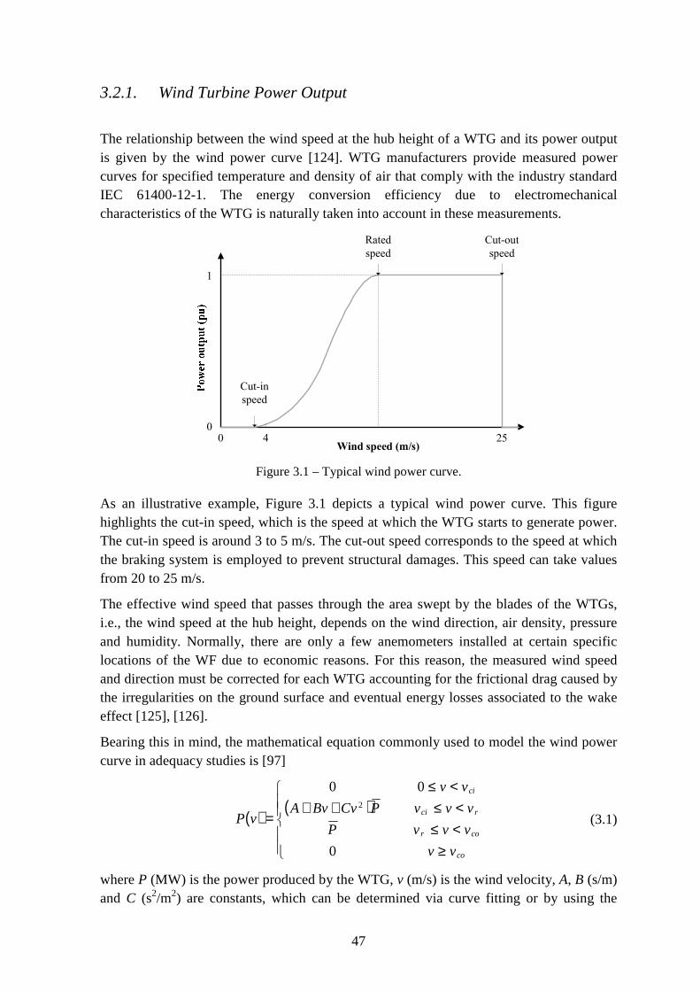
47

3.2.1. Wind Turbine Power Output

The relationship between the wind speed at the hub height of a WTG and its power output is given by the wind power curve [124]. WTG manufacturers provide measured power curves for specified temperature and density of air that comply with the industry standard IEC 61400-12-1. The energy conversion efficiency due to electromechanical characteristics of the WTG is naturally taken into account in these measurements.

Figure 3.1 – Typical wind power curve.

As an illustrative example, Figure 3.1 depicts a typical wind power curve. This figure highlights the cut-in speed, which is the speed at which the WTG starts to generate power. The cut-in speed is around 3 to 5 m/s. The cut-out speed corresponds to the speed at which the braking system is employed to prevent structural damages. This speed can take values from 20 to 25 m/s.

The effective wind speed that passes through the area swept by the blades of the WTGs, i.e., the wind speed at the hub height, depends on the wind direction, air density, pressure and humidity. Normally, there are only a few anemometers installed at certain specific locations of the WF due to economic reasons. For this reason, the measured wind speed and direction must be corrected for each WTG accounting for the frictional drag caused by the irregularities on the ground surface and eventual energy losses associated to the wake effect [125], [126].

Bearing this in mind, the mathematical equation commonly used to model the wind power curve in adequacy studies is [97]

( ) ( )

≥<≤<≤++

<≤

=

co

cor

rci

ci

vv

vvvP

vvvPCvBvA

vv

vP

0

002

(3.1)

where P (MW) is the power produced by the WTG, v (m/s) is the wind velocity, A, B (s/m) and C (s2/m2) are constants, which can be determined via curve fitting or by using the

Wind speed (m/s)2540

1

Cut-in

speed

Cut-out

speed

Rated

speed

0

48

equations deduced in [97], vci (m/s) is the cut-in wind speed, vr (m/s) is rated speed and vco (m/s) is the cut-out speed. As an illustrative example, Figure 3.2 depicts the power produced by a typical WTG for a wind regime of 24 hours. This figure shows that small changes in wind speed can result in high variations in the power output of a WTG.

Figure 3.2 – Wind power output of a WTG as function of the wind speed.

WTGs can experience forced outages. For that reason, the power output of a WF is a result of two stochastic processes:

• The wind speed intermittency, which is non-stationary a continuous physical phenomenon that evolves randomly in time and space [123];

• Forced outages due to electrical or structural failure, which is a stationary process usually modeled by the two-state Markov model.

When a WTG is available, i.e., in the up state, the power output for every wind speed realization is given by the wind power curve. Conversely, the power output is zero when in the down state. Despite this, studies have shown that the failure/repair cycle of WTGs can be neglected in many practical applications without creating unreasonable errors in the reliability indices [127]. Generally, these two stochastic processes are assumed independent, i.e., the availability of the WTG does not depend on the wind regime. However, forced outages tend to occur more often in windy periods [123]. These faults are more catastrophic in nature, such as cracking of the tower and blades, which imply lengthy repair times. Therefore, different stochastic parameters should be used for different wind speeds.

3.2.2. Wind Power Series vs. Wind Speed Series

Most of the fluctuating behavior of wind power is caused by wind intermittency, which can have hourly, daily, seasonally or even yearly patterns. The adequacy models traditionally used to capture this stochastic behavior can be divided according to the type of data on

0

0.2

0.4

0.6

0.8

1

1.2

0

5

10

15

20

25

30

0:00 2:24 4:48 7:12 9:36 12:00 14:24 16:48 19:12 21:36 0:00

pum/s

hr

Wind Power Wind Speed

49

which they are based [128]. Hence, there are models based on wind power [53], [54] or on wind speed data [129], [130]. The power curve of the WTGs can be used to convert wind speed data into power realizations. However, this conversion process is strongly discouraged since the nonlinearity of the wind power curve can greatly increase measurement errors.

Models based on wind power measurements are the most straightforward. They use historical data collected from the Supervisory Control and Data Acquisition (SCADA) systems over several years. Conversely, the models based on wind speed can either use historical or synthetically generated data [130–133]. The ability of several numerical and/or statistical approaches, like autoregressive models [130], [134] and Markov chains [131–133] to provide representative synthetic wind speed series has been the subject of considerable investigation. Since synthetically generated data can fail to accurately capture the time-dependency of wind, the use of synthetic speeds is only justified when there are few measurements available. The first wind models used in the adequacy assessment of power systems were based on wind speed data [97], [123].

The wind intermittency can be modeled for each WTG or for the whole WF. For the sake of accuracy, it is preferable to use data for each WTG. When WFs encompass a large number of WTGs or when data for each WTG is impossible to be obtained, the use of data for the whole WF is justifiable. This approximation allows saving considerable memory space especially in the case of large WFs. In the case of farms with few WTGs, this approximation must be used parsimoniously.

It is worth mentioning that the correct modeling of the wind intermittency depends on the quality of the data collected. The minimum amount of data necessary to obtain accurate estimates of the reliability indices is only possible to be estimated by a trial and error process. Nonetheless, an adequacy assessment study for the Irish system [135] has shown that at least four to five years of data in an hourly resolution are mandatory.

3.2.3. Wind Farm Models

The models of WFs used in power system adequacy assessment can be divided into state space-based models and sequential-based models. When significant historical information is available, the direct use of wind speed or wind power series in the sequential MCS method, i.e., the use of sequential models, is the most straightforward approach since this method can synthetically create the chronological operation of the system.

Every year simulated can use a series, which represents a yearly regime, by making a random sampling from all series available according to their respective probability of occurrence. Since these series encompass several years of observations, they can naturally model the hourly, diurnal, seasonal and yearly patterns of wind. Moreover, temporal and spatial correlations between different WFs are inherently accounted for. These series can be available for the whole WF or for every WTG.

50

Unfortunately, the sequential models cannot be directly used in analytical and non-sequential MCS methods, which are computationally more attractive alternatives to the sequential MCS method. For that reason, several authors have proposed state space-based models [123], [127], [136], [137]. Their main disadvantage is that they cannot easily incorporate the time-dependent nature of wind.

A possible way to address this issue is to use clusters of load and wind speed realizations [138], [139]. The load and speed over a given period of time, for instance over an hour, can be understood a single data point. Similar data points can be clustered by using the nearest centroid sorting algorithm based on the Euclidean distance. The probability and frequency of occurrence of each cluster, which is represented by a mean load and a mean speed, can then be used in the analytic and in the non-sequential MCS methods. Besides this clustering method, the correlation of wind and load can be captured by evaluating the different periods of time within a year separately (e.g. every month) [137]. The reliability indices obtained for each period are then added to obtain their annual value. Despite the soundness of these two approaches, they cannot provide the correct value of the frequency and duration indices. Clearly, sequential models are the most accurate way to incorporate the wind intermittency into the adequacy studies.

3.2.3.1. State Space-based Models

The first state space models were proposed to be used by analytical-based adequacy assessment methods [123]. These models were built upon wind speed series. The first ones relied on first-order time-homogenous Markov chains to model the transitions of the wind speed between a finite set of states. Figure 3.3 depicts a Markov chain composed of five wind speed states. In this figure, the state v1 corresponds to the lowest speed and state v5 to the highest.

Figure 3.3 – Markov chain for modeling the wind speed.

The first-order time-homogenous Markov chains have three important assumptions [123]. The first assumption is related to the fact that the occurrence of the next wind state only depends on the actual state. This assumption has been tested and experiments have proven that high-order processes are more suitable to capture the time-dependency of wind speed [131]. Second, one is assuming that, by using a time-homogenous process, the stochastic behavior of the wind speed is not affected by seasonal patterns, i.e., the mean speed and respective standard deviation is the same regardless of the timespan of the data. This assumption is clearly against the non-stationary nature of wind. Third, , one is considering that, according to the Markov property, the state residence time follows a geometric distribution, in the case of discrete-time Markov chains, or an exponential distribution, in case of continuous chains. The literature has demonstrated that semi-Markov [133]

51

processes, which allow transitions between states according to any probability distribution, can reproduce the statistical properties of wind speed better than Markov processes. However, the exponential assumption is valid when the objective is to obtain the limiting probabilities and frequencies of the states and not to reproduce the time-dependency of the underlying stochastic process [123].

To create a first-order time-homogenous Markov chain for the wind speed, a finite number of states from the continuous range of observed wind speeds must be extrapolated. The wind speed of these states does not need to be equally spaced. The precision of the discretization process defines the number of states. Since the complexity of the state space model increases as the number of states of the Markov chain grows, the discretization step must be carefully chosen, i.e., the number of wind speed states obeys to a tradeoff between computational performance and accuracy. Clustering techniques [127] for aggregating similar wind speeds into groups can be used to obtain an appropriate number of states.

After the discretization process, the transition rate between two wind speed states can be calculated [123] using

i

ijij

D

N=λ (3.2)

where λij is the transition rate between state i and state j, Nij is the number of transitions from state i to state j and Di is the duration of state i, which is given by the sum of durations of all N time intervals in which state i has occurred [123] as

∑=

=N

k

ki tD1

. (3.3)

The probability of occurrence of state [123] is given by

S

ii

D

DP = (3.4)

where DS is the length of the wind speed series. The accurate estimation of these parameters is only possible when the number of interstate transitions is sufficiently large [123].

The model depicted in Figure 3.3 does not allow transitions between nonadjacent states. According to the authors of this model [123], all intermediate states must be encountered when moving from different wind speed levels even if these transitions are not detected. Given the fact that the wind speed is measured at fixed instants of time, other authors have argued that transitions between nonadjacent states should be modeled [127]. The transitions between nonadjacent states account for large speed variations in small time intervals.

Figure 3.4 illustrates a Markov chain that allows direct transitions between calm and windy states. Like Figure 3.3, the state v1 corresponds to the lowest wind speed whereas state v5 represents the highest.

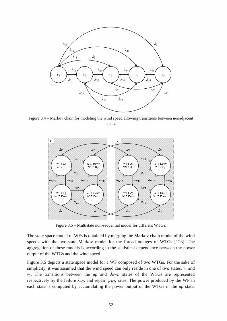
52

Figure 3.4 – Markov chain for modeling the wind speed allowing transitions between nonadjacent states.

Figure 3.5 – Multistate non-sequential model for different WTGs.

The state space model of WFs is obtained by merging the Markov chain model of the wind speeds with the two-state Markov model for the forced outages of WTGs [123]. The aggregation of these models is according to the statistical dependence between the power output of the WTGs and the wind speed.

Figure 3.5 depicts a state space model for a WF composed of two WTGs. For the sake of simplicity, it was assumed that the wind speed can only reside in one of two states, v1 and v2. The transitions between the up and down states of the WTGs are represented respectively by the failure λWT, and repair, µWT, rates. The power produced by the WF in each state is computed by accumulating the power output of the WTGs in the up state.

v1 v2 v3 v4 v5

λ12 λ23

λ21 λ32

λ34

λ34

λ45

λ54

λ15 λ51

λ41

λ31

λ14

λ13

λ25 λ52

λ24 λ42

λ35 λ53

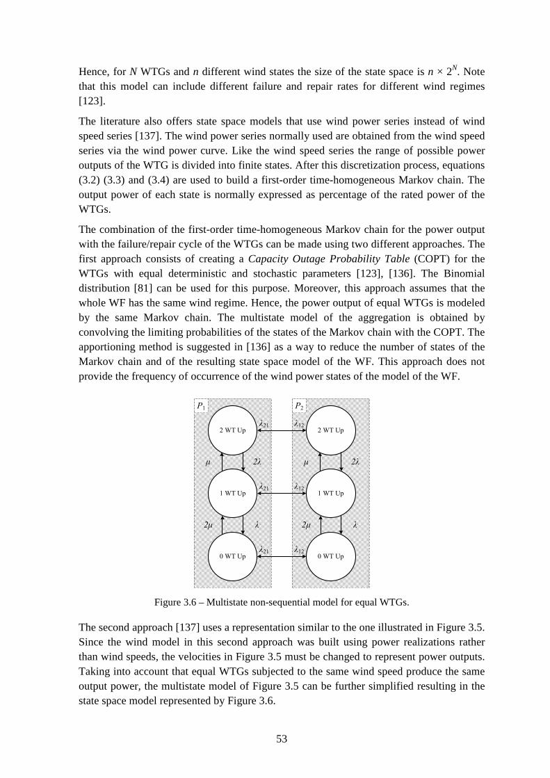
53

Hence, for N WTGs and n different wind states the size of the state space is n × 2N. Note that this model can include different failure and repair rates for different wind regimes [123].

The literature also offers state space models that use wind power series instead of wind speed series [137]. The wind power series normally used are obtained from the wind speed series via the wind power curve. Like the wind speed series the range of possible power outputs of the WTG is divided into finite states. After this discretization process, equations (3.2) (3.3) and (3.4) are used to build a first-order time-homogeneous Markov chain. The output power of each state is normally expressed as percentage of the rated power of the WTGs.

The combination of the first-order time-homogeneous Markov chain for the power output with the failure/repair cycle of the WTGs can be made using two different approaches. The first approach consists of creating a Capacity Outage Probability Table (COPT) for the WTGs with equal deterministic and stochastic parameters [123], [136]. The Binomial distribution [81] can be used for this purpose. Moreover, this approach assumes that the whole WF has the same wind regime. Hence, the power output of equal WTGs is modeled by the same Markov chain. The multistate model of the aggregation is obtained by convolving the limiting probabilities of the states of the Markov chain with the COPT. The apportioning method is suggested in [136] as a way to reduce the number of states of the Markov chain and of the resulting state space model of the WF. This approach does not provide the frequency of occurrence of the wind power states of the model of the WF.

Figure 3.6 – Multistate non-sequential model for equal WTGs.

The second approach [137] uses a representation similar to the one illustrated in Figure 3.5. Since the wind model in this second approach was built using power realizations rather than wind speeds, the velocities in Figure 3.5 must be changed to represent power outputs. Taking into account that equal WTGs subjected to the same wind speed produce the same output power, the multistate model of Figure 3.5 can be further simplified resulting in the state space model represented by Figure 3.6.

2 WT Up

1 WT Up

0 WT Up

P1

2λµ

λ2µ

2 WT Up

1 WT Up

0 WT Up

P2

2λµ

λ2µ

λ21 λ12

λ21 λ12

λ12λ21

54

Now, if the discretization of the wind power series was made assuming that the equally wind power states are equally spaced, the state P2 in Figure 3.6 is a multiple of P1. Therefore, some states in Figure 3.6 correspond to the same wind power produced by the WF. For instance, if P2 is equal to 2 × P1, there are two states in this figure that result in the power output P2.

Taking this into account, the authors of [137] proposed a second discretization process for the whole range power outputs of the WF, which, in the case of Figure 3.6, is the discrete interval between 0 and 2 × P2. This new multistate Markov model, which has unique power output states for the WF, is obtained using probability analysis techniques, which calculate the probability and frequency of the wind output states of the WF and the respective transition rates between them.

The state space models previously described can be used by analytical methods and by the non-sequential MCS method. In the case this last method, it is possible to use simpler WF models [83]. As such, the straightforward way to model the power output of a WTG in non-sequential MCS method is to sample, first, a wind speed from its probability distribution (for instance, from the two parameter Weibull distribution or from the frequency distribution defined by the wind speed measurements) and, second, the availability of the WTGs. If a WTG is in the up state, the wind power curve is used to determine its power output. Conversely, if a WTG is in the down state, the power output is zero. The total power generated by the WF is obtained by adding the individual contribution of each WTG. Special test functions were developed to estimate frequency and duration reliability indices including WFs [16].

3.2.3.2. Sequential-based Models

The first wind speed-based sequential model proposed relies on the Autoregressive Moving Average (ARMA) model [129]. The parameters of the ARMA model used are estimated using wind speed observations over several years. The samples from the ARMA model are based on hourly observed means and standard deviations. The power produced by the WF is obtained by adding the individual contribution of each WTG according to their availability and respective wind power curve.

An alternative sequential model, which also uses an ARMA model for sampling hourly wind speeds, has been proposed recently [113]. In this case, a power curve for the entire WF is used instead of a curve for each WTG. This aggregated power curve is created by sampling hourly wind speeds from the ARMA model and calculating the respective power output realizations of the WF using the power curve of the WTGs. The resulting hourly power outputs are plotted against the underlying wind speeds to create a power curve for the WF. The parameters of this aggregated curve are estimated using curve fitting analysis. This sequential model does not explicitly state how forced outages of WTGs are accounted for.

55

The literature in HL1 studies with wind power offers a simple sequential model based on wind power measurements [53], [54]. This model assumes that each WTG in the up state contributes equally the hourly output of the WF. The wind intermittency is captured by wind power series that represent the hourly output of the farm as percentage of its rated capacity. Since most WTGs of WFs are equal, this approach enables the use of the multistate Markov model for the representation of the stochastic failure/repair cycle of the whole WF. Hence, by identifying the number of WTGs in the up state, the hourly power output of the WF can be easily obtained by a simple multiplication operation.

3.3. Inertial Constraint

Wind power curtailment evens can occur at low penetration levels due to transmission bottlenecks. On the other hand, these events tend to occur more often at high penetration levels when a windy condition coincides with a period of low demand. One justification for this is the higher dispatching priority given by the system operators to more stable generating units over WFs. To account for this operational procedure, a simple model is proposed in this dissertation. This model consists of guaranteeing that a given amount of load, designated as inertial load, is always supplied by a fixed set of generating units regardless of the hourly load variation. It finds inspiration in the concept of must-run units [140], [141], which are generating facilities that need to be online during certain operating conditions in order to maintain the stability, security, and continuity of supply. Note that the security and stability are broad concepts for the model proposed and do not refer to a specific dynamic problem. For that reason, it is assumed that the set of generating units, which have certain dynamic characteristics, is capable of ensuring rotor, frequency and voltage stability as long as the inertial load is supplied by them. Note that the security of the system depends on the dynamic characteristics of the generating units scheduled for operation, as well as some procedures adopted by the system operator. Only through dynamic assessment studies it is possible to determine the actual security of the system.

The inertial load and the units capable of supplying it depend on the characteristics of the system. The value of the inertial load must be set according to the dynamic characteristics of the generating units available and the operational procedures adopted by the system operator. New WFs in the system will certainly influence its dynamic behavior and, consequently, the value of inertial load. Clearly, the inertial constraint model is a simple approximation for the long-term adequacy assessment of the composite system that accounts for security issues when making the dispatch of the generating units.

Some system operators use similar procedures that are in line with the assumptions of the proposed model. In the glossary2 of terms and acronyms of the California Independent System Operator (ISO), California ISO, the following definitions can be found:

• Reliability Must-Run Contract : a must-run service agreement between the owner of a Reliability Must-Run Unit and the California ISO;

2 http://www.caiso.com/Pages/glossary.aspx [accessed in 22/11/2012].

56

• Reliability Must-Run Unit : a generating unit of a participating generator which is the subject of a Reliability Must-Run Contract;

• Reliability Must-Run Generation: generation that the California ISO determines is required to be on line to meet Applicable Reliability Criteria requirements. This includes:

� Generation constrained on line to meet North America Reliability Council (NERC) and Western Electricity Coordinating Council (WECC) reliability criteria for interconnected systems operation;

� Generation needed to meet load demand in constrained areas;

� Generation needed to be operated to provide voltage or security support of the California ISO or a local area;

• Applicable Reliability Criteria : the Reliability Standards and Reliability Criteria established by NERC and WECC and local reliability criteria, as amended from time to time, including any requirements of the Nuclear Regulatory Commission;

• Reliability Standard : A requirement approved by Federal Energy Regulatory Commission (FERC) under Section 215 of the Federal Power Act to provide for reliable operation of the bulk power system. The term includes requirements for the operation of existing bulk power system facilities, including cyber security protection, and the design of planned additions or modifications to such facilities to the extent necessary for reliable operation of the bulk power system. This term does not include any requirement to enlarge such facilities or to construct new transmission capacity or generating capacity;

• Reliability Criteria : pre-established criteria that are to be followed in order to maintain desired performance of the California ISO controlled grid under contingency or steady state conditions.

This model, henceforth called inertial constraint, is enforced even when there is not enough generating capacity to supply the inertial load (for instance, due to forced outages). When such an event occurs, the inertial load is set to the maximum capacity available and the event is marked as an insecure state. This concept of insecure state is used to monitor the events when the total capacity of the fixed set of generating units is insufficient to attend the inertial load. Similarly to the loss of load events, the concept of reliability indices can be extended to characterize insecure state events, as follows:

• Insecure State Probability - ISP, probability of an insecure state event;

• Insecure State Expectation - ISE, average number of hours in which insecure states occur (hour/year);

• Expected Inertial Load Not Supplied - EILNS, expected power by which the set of generating units fail to supply the inertial load (MW);

• Insecure State Frequency - ISF, average frequency of insecure state events (occurrence/year);

57

• Insecure State Duration - ISD, average duration of insecure state events (hour/occurrence).

3.4. Wind Power Curtailment Events

The following types of events that can limit the use of the total wind power available are analyzed in this dissertation:

• Event A: wind power curtailment due to the enforcement of the inertial constraint and/or load deficit;

• Event B: wind power curtailment due to transmission circuit failures and/or capacity limits;

• Event C: wind power curtailment due to the simultaneous occurrence of events A and B.

These events are captured when there no load is curtailed since, when such a corrective measure is adopted, system operators are interested in minimizing the total loss of load or the loss of load cost even if it leads to wind power disconnection.

The maximum wind capacity that can be used is upper-bounded by the difference between the hourly load and the load supplied by the units of the inertial constraint. This difference is named as Maximum Usable Wind Capacity (MUWC).

If, after evaluating the system state, there is Wind Capacity Curtailed (WCC) and no loss of load, then the Total Wind Capacity Available (TWCA) is compared with the MUWC. If the TWCA is less than or equal to the MUWC, then the wind power curtailment is due to transmission circuit failures and/or capacity limits (i.e., an Event B has occurred).

On the contrary, if the TWCA is greater than the MUWC, then the WCC is checked. If the WCC is equal to the difference between the TWCA and the MUWC, then the wind power curtailment is due to the enforcement of the inertial constraint and/or load deficit (i.e., an Event A has occurred). Otherwise, if the WCC is greater than the difference between the TWCA and the MUWC, then the wind power curtailment is due to the simultaneous occurrence of events A and B (i.e., an Event C has occurred).

Similarly to the insecure state events, it is possible to define a set of indices to characterize wind power curtailment events, such as:

• Loss of Wind Power Probability - LOWP, probability of wind power curtailment event;

• Loss of Wind Power Expectation - LOWE, average number of hours in which wind power curtailment events occur (hour/year);

• Expected Wind Power Curtailed - EWPC, average wind power curtailed (MW);

58

• Expected Wind Energy Curtailed - EWEC, average wind energy curtailed (MWh/year);

• Wind Power Curtailment Frequency - WPCF, average frequency of wind power curtailment events (occurrence/year);

• Wind Power Curtailment Duration - WPCD, average duration of wind power curtailment events (hour/occurrence).

These indices can also be determined for the three types of wind power curtailment events.

As a last remark, note that the LOWP index refers to the probability of the events when the wind power available is not totally used due to dispatch and/or load deficit, to transmission bottlenecks or to the simultaneous occurrence of both. The events with no wind power due to wind speed characteristics of each WTG (e.g., cut-in and cut-off speeds) or simply no wind speed are not considered by this index.

3.5. Detection of Wind Power Curtailment Events

The evaluation of a composite state comprises the execution of three tasks (see section 2.9.2.2). As mentioned earlier, the first task consists of dispatching the hourly load to the available generating units taking into account their operating limits. After that, a DC PF analysis is performed to check whether loading limits of the transmission lines and transformers are violated. Finally, if there are limits violated, a DC OPF is run.

To take into account the inertial constraint in the dispatch of the generating units, it is necessary to check if there is enough generating capacity within the set to meet this requirement. If there is, the generating units of the inertial constraint are dispatched with the inertial load. If there is not, these units are dispatched at their full capacity and this event is marked as insecure. The difference between the hourly load and the inertial load is dispatched to other available generating units according to a merit order strategy. WFs always have the highest merit.

A DC OPF is run whenever transmission circuits with violated loading limits are detected by the DC PF. This task consists of enforcing the operating limits of system components by altering the real power injected at buses, by solving

max. ∑∑ −=j

jGFi

iGW PMPzj (3.5a)

s. t. LGF PP0 ≤≤ (3.5b)

GGG PPP ≤≤ (3.5c)

ikik PΓZθP ≤≤ (3.5d)

0θBPPP =+−+ 'LGFG (3.5e)

59

ICk

kGIC PP ≥∑ (3.5f)

where PGF is the vector of real power produced by the fictitious generating units that model the load curtailment, Mj is a constant that reflects the load curtailment priority of the load at bus j, PGW is the vector of the real power produced by the WFs, PG is the vector of the real power produced by the generating units, PL is the vector of real power consumption, Г is a diagonal matrix whose entries are the inverse of the branches’ reactance, Z is the branch-bus incidence matrix, θ is the vector of bus voltage angles, B' is the susceptance matrix of the DC PF, PGIC is a vector that contains the power produced by the set of generating units capable of supplying the inertial load and PIC is the inertial load.

3.6. Impact of Transmission Circuits on Wind Power Curtailment

When a transmission circuit violates its operating limits, remedial actions are taken. If the power system is represented by a linearized power flow, or simply, by a DC PF model, the remedial actions (e.g., generation redispatch and/or load curtailment) are enforced by solving a linear optimization problem. The objective of this optimization problem is to minimize the total loss of load subjected to the operating limits of generating units and transmission circuits, and to the DC PF equations.

Nonetheless, the objective of this optimization problem can be changed to give preference of some generating units over others without modifying the estimates of the composite system reliability indices. Bearing this in mind, the maximization of the use of wind power and the minimization of the loss of load can be aggregated in the same objective function by using appropriate weights [5], [9]. These weights must be established according to the importance of each objective [5], [9].

After solving the linear optimization problem, the dual variables associated with each constraint become available. Using the objective function proposed in the last paragraph and assuming that a wind power curtailment event has occurred, the dual variables express the increase in the use of wind power if the resource modeled by the constraint is augmented in its capacity by one unit. As transmission circuits are subject to failures, this incremental result can be obtained by calculating the difference between the dual variables of the buses at their extremes, in the same way as the sensitivity analysis regarding circuit reinforcement [5]. These dual variables are taken from with the equality constraints of the DC PF equations (3.5e). In mathematical terms

kiik πππ −= (3.6)

where, πik is the dual variable associated to the transmission circuit connecting buses i to k and πi = ∂z / ∂Pi, where z is the objective function and Pi is the injected power of bus i.

When πik is different from zero, the circuits involved in the wind curtailment events B and C can be detected, making it possible to obtain yearly statistics for each circuit, such as the

60

cumulative probability distribution of the wind power curtailed when the circuit is limiting the use of the total wind capacity available.

3.7. Composite System Adequacy Assessment including the Maximization of the Use of Wind Power

The discussion of the results of the experiments carried out in this chapter is divided into two parts. The first part consists of analyzing which criteria should be used to compare different technologies based on their contribution to the composite system adequacy. The inertial constraint is not considered in this analysis. The experiments carried out in this part are based on two configurations of the IEEE-RTS 79 [91] test system, namely the IEEE-RTS 79 HW and IEEE-RTS 79 HT. The main difference between these two configurations is that the IEEE-RTS 79 HW includes three WFs whereas IEEE-RTS 79 HT system has a thermal unit of 400 MW. The second part of the discussion of the results aims to investigate the events that limit the use of the total wind capacity available. In this case, three sets of experiments are proposed. The first set was conceived to investigate the influence of the inertial constraint on the system adequacy. Therefore, four configurations of the IEEE-RTS 79 HW system with 400 MW of wind capacity were evaluated considering four different values of the inertial load:

• Configuration IL1: 95% of the valley load;

• Configuration IL2: 75% of the valley load;

• Configuration IL3: 50% of the valley load;

• Configuration IL4: 25% of the valley load.

The second set was planned to determine how wind curtailment events are influenced by the levels of wind penetration, which type of wind curtailment event occurs more often and which transmission circuits are limiting the use of total wind power available. These experiments are conducted on the IEEE-RTS 79 HW configurations IL1 and IL2 for two extreme scenarios of wind power capacity installed: 400 MW and 1200 MW. Finally, the third set of experiments was devised to demonstrate the effect of that stressed transmission systems have on wind power curtailment events. For this purpose, the generation capacity and the system load of the IEEE-RTS 79 HW 400 MW and 1200 MW of wind capacity configurations was increased by a factor of 1.5. As a result, the wind capacity in the configurations of the IEEE-RTS 79 HW increased from 400 MW to 600 MW and from 1200 MW to 1800 MW respectively. The inertial load used was 75% of the valley load.

3.7.1. Test Systems

The IEEE-RTS 79 HW results from modifications on the IEEE-RTS 79 system to account for the variability of hydro capacity and to include wind power. The first modification

61

consisted on allowing the 300 MW of hydro capacity to vary in a monthly basis according to five historical series. These series are available in [54] and correspond to those of Area 1. All series have the same probability of occurrence.

The second and final modification consisted on adding three WFs. The WFs are composed of WTGs of 2 MW, which have an MTTF = 1914.74 h and a MTTR = 80 h, and are connected to buses 8, 11 and 19. The WFs at bus 8 and 11 contribute each one with 30% to the share of wind capacity in the system. Conversely, the WF at bus 19 is 40% of the total. Each WF has three output power series with an hourly resolution. The probabilities of occurrence are 33.34%, 33.33% and 33.33%, respectively. These series can be obtained from [54]. The series of the WF at bus 8 correspond to those of Area 1. The series of the WF at bus 11 are those of Area 2. Finally, bus 19 WF series are those of Area 3. The set of units that can supply the inertial constraint are the four 155 MW units, the 350 MW unit, and the two 400 MW units of the original configuration of the IEEE-RTS 79.

The IEEE-RTS 79 HT configuration relies on the same modifications proposed for the hydro units of the IEEE-RTS 79 HW. In addition, a 400 MW thermal generator, which has a MTTF = 1100 h and a MTTR = 150 h, is connected to bus 19.

The hourly load model of the configurations HW and HT of the IEEE-RTS 79 test system include the 28th day of February, by copying the twenty-four hourly peaks of the previous day.

3.7.2. Analysis of the Wind and Thermal Technologies

To investigate the wind and thermal contribution to the adequacy of the composite system, the reliability indices of the IEEE-RTS 79 HT were obtained. After that, several configurations of the IEEE-RTS 79 HW were evaluated, each one containing an increasing amount of wind installed capacity, to determine the installed capacity at which the three WFs are able to provide the same composite adequacy as the 400 MW thermal unit. The evaluations were stopped when the estimates of the reliability indices had a coefficient of variation less than or equal to 5%. The results of the proposed experiments are presented in Table 3.3 and Table 3.4.

Apart from the composite adequacy reliability indices, the Annual Maximum Energy (AME) of the generating units was monitored. This performance measure can be calculated using

∫=

=

=8760

0

)(AMEt

t

G dttP (3.7)

where )(tPG is the maximum generating capacity of a given unit at the instant of time t.

The different AME realizations obtained for each year simulated can be averaged to obtain the Expected Annual Maximum Energy (EAME) as

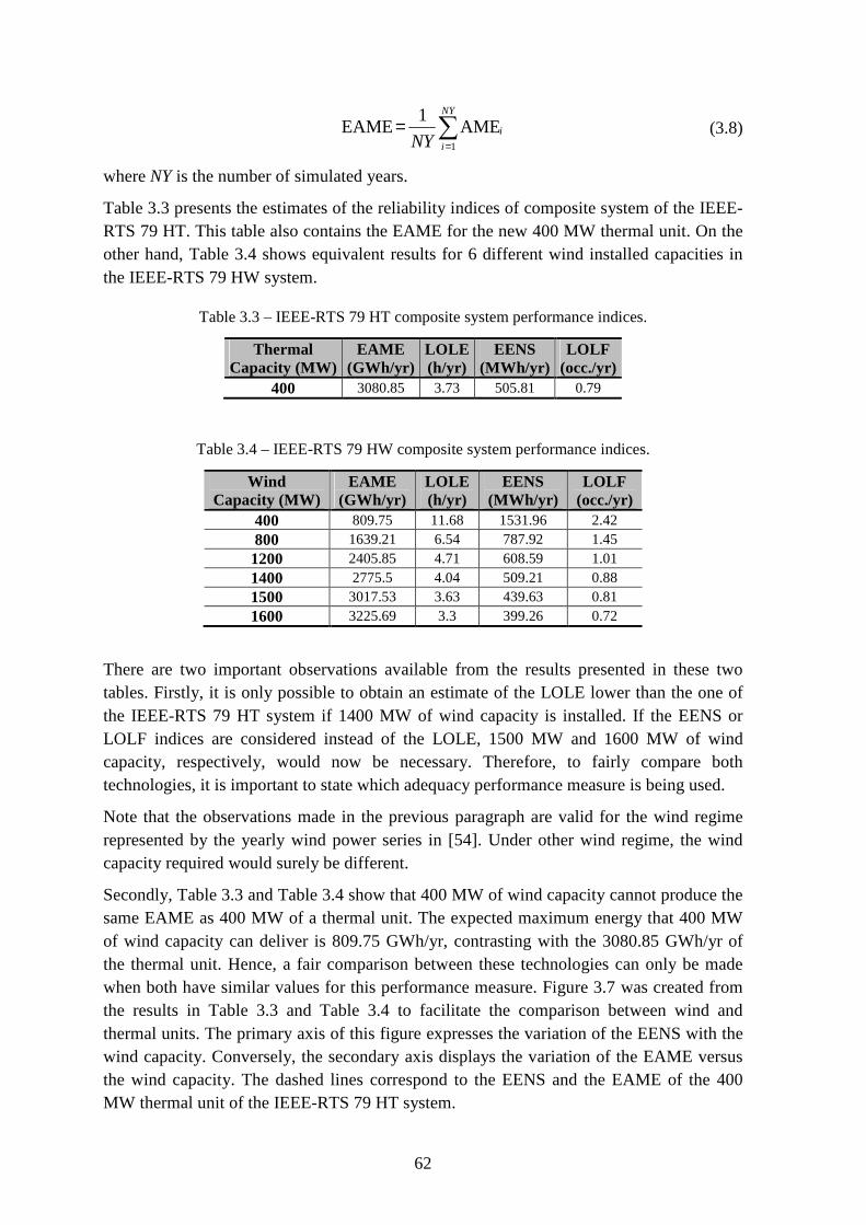
62

∑=

=NY

i

iNY 1

AME1

EAME (3.8)

where NY is the number of simulated years.

Table 3.3 presents the estimates of the reliability indices of composite system of the IEEE-RTS 79 HT. This table also contains the EAME for the new 400 MW thermal unit. On the other hand, Table 3.4 shows equivalent results for 6 different wind installed capacities in the IEEE-RTS 79 HW system.

Table 3.3 – IEEE-RTS 79 HT composite system performance indices.

Thermal Capacity (MW)

EAME (GWh/yr)

LOLE (h/yr)

EENS (MWh/yr)

LOLF (occ./yr)

400 3080.85 3.73 505.81 0.79

Table 3.4 – IEEE-RTS 79 HW composite system performance indices.

Wind Capacity (MW)

EAME (GWh/yr)

LOLE (h/yr)

EENS (MWh/yr)

LOLF (occ./yr)

400 809.75 11.68 1531.96 2.42 800 1639.21 6.54 787.92 1.45 1200 2405.85 4.71 608.59 1.01 1400 2775.5 4.04 509.21 0.88 1500 3017.53 3.63 439.63 0.81 1600 3225.69 3.3 399.26 0.72

There are two important observations available from the results presented in these two tables. Firstly, it is only possible to obtain an estimate of the LOLE lower than the one of the IEEE-RTS 79 HT system if 1400 MW of wind capacity is installed. If the EENS or LOLF indices are considered instead of the LOLE, 1500 MW and 1600 MW of wind capacity, respectively, would now be necessary. Therefore, to fairly compare both technologies, it is important to state which adequacy performance measure is being used.

Note that the observations made in the previous paragraph are valid for the wind regime represented by the yearly wind power series in [54]. Under other wind regime, the wind capacity required would surely be different.

Secondly, Table 3.3 and Table 3.4 show that 400 MW of wind capacity cannot produce the same EAME as 400 MW of a thermal unit. The expected maximum energy that 400 MW of wind capacity can deliver is 809.75 GWh/yr, contrasting with the 3080.85 GWh/yr of the thermal unit. Hence, a fair comparison between these technologies can only be made when both have similar values for this performance measure. Figure 3.7 was created from the results in Table 3.3 and Table 3.4 to facilitate the comparison between wind and thermal units. The primary axis of this figure expresses the variation of the EENS with the wind capacity. Conversely, the secondary axis displays the variation of the EAME versus the wind capacity. The dashed lines correspond to the EENS and the EAME of the 400 MW thermal unit of the IEEE-RTS 79 HT system.

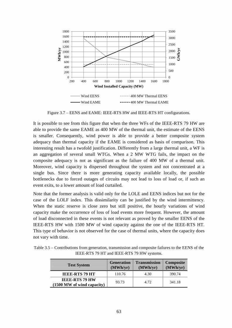
63

Figure 3.7 – EENS and EAME: IEEE-RTS HW and IEEE-RTS HT configurations.

It is possible to see from this figure that when the three WFs of the IEEE-RTS 79 HW are able to provide the same EAME as 400 MW of the thermal unit, the estimate of the EENS is smaller. Consequently, wind power is able to provide a better composite system adequacy than thermal capacity if the EAME is considered as basis of comparison. This interesting result has a twofold justification. Differently from a large thermal unit, a WF is an aggregation of several small WTGs. When a 2 MW WTG fails, the impact on the composite adequacy is not as significant as the failure of 400 MW of a thermal unit. Moreover, wind capacity is dispersed throughout the system and not concentrated at a single bus. Since there is more generating capacity available locally, the possible bottlenecks due to forced outages of circuits may not lead to loss of load or, if such an event exits, to a lower amount of load curtailed.

Note that the former analysis is valid only for the LOLE and EENS indices but not for the case of the LOLF index. This dissimilarity can be justified by the wind intermittency. When the static reserve is close zero but still positive, the hourly variations of wind capacity make the occurrence of loss of load events more frequent. However, the amount of load disconnected in these events is not relevant as proved by the smaller EENS of the IEEE-RTS HW with 1500 MW of wind capacity against the one of the IEEE-RTS HT. This type of behavior is not observed for the case of thermal units, where the capacity does not vary with time.

Table 3.5 – Contributions from generation, transmission and composite failures to the EENS of the IEEE-RTS 79 HT and IEEE-RTS 79 HW systems.

Test System Generation (MWh/yr)

Transmission (MWh/yr)

Composite (MWh/yr)

IEEE-RTS 79 HT 110.76 4.30 390.74

IEEE-RTS 79 HW (1500 MW of wind capacity)

93.73 4.72 341.18

0

500

1000

1500

2000

2500

3000

3500

0

200

400

600

800

1000

1200

1400

1600

1800

200 400 600 800 1000 1200 1400 1600 1800

GW

h/yr

MW

h/yr

Wind Installed Capacity (MW)

Wind EENS 400 MW Thermal EENS

Wind EAME 400 MW Thermal EAME

64

Table 3.5 presents the contributions of the generation, transmission and composite failures to the EENS of the IEEE-RTS 79 HT and of the IEEE-RTS 79 HW with 1500 MW of wind capacity. These two configurations were selected for comparison since the EAME of the wind and thermal capacities are similar (see Table 3.4). The results presented in this table show that the better EENS of the 1500 MW of wind IEEE-RTS 79 HW over the one of the IEEE-RTS 79 HT results from a decrease in generation and composite failures. Conversely, the contribution of transmission failures to the EENS is similar. From these observations one can conclude that the granularity of the wind capacity has a greater importance than its dispersed nature in the better adequacy of 1500 MW of wind power over 400 MW of thermal capacity.

3.7.3. Analysis of the Wind Power Curtailment Events

As stated previously, the first set of experiments proposed for this section aims to analyze the influence of the inertial constraint on the composite system adequacy. Therefore, four runs of the IEEE-RTS 79 HW configuration with 400 MW of wind capacity were carried out considering four different values for the inertial load. Table 3.6 presents the insecure state indices obtained for these four configurations.

Table 3.6 – Insecure state indices vs. inertial load.

IEEE-RTS 79 HW (400 MW of wind capacity)

ISE (h/yr)

EILNS (MW)

ISF (occ./yr)

IL 1 48.19 0.71 1.72

IL 2 11.94 0.15 0.38 IL 3 1.24 4.81×10-3 6.30×10-2 IL 4 6.86×10-3 6.76×10-5 8.34×10-4

First, the results in Table 3.6 show that the reliability indices of the composite system of the configurations of the IEEE-RTS 79 HW simulated remain the same (LOLE = 11.68 h/y, EENS = 1531.96 MWh/y, and LOLF = 2.42 occ./y) regardless of the value of the inertial load. Therefore, solving the optimization problem formulated in (3.5) leads to the same estimates of the reliability indices as the traditional formulation proposed in (2.40).

Moreover, the results in Table 3.6 demonstrate that, as the inertial load increases, the occurrence of insecure states becomes more frequent. Despite this increase, the expected power by which the fixed set of generation units fails to supply the inertial load (i.e., the EILNS index) is not significant when compared to the capacity of the generating units in the set or even the inertial load. This shows that the number of generating units in the set is appropriate to guarantee a continuous supply of the inertial load.

One of the objectives of the second set of experiments is to identify which type of wind curtailment event occurs more often. For this purpose, the wind curtailment indices of the IEEE-RTS 79 HW configurations IL1 and IL2 considering two extreme scenarios of wind power capacity installed (400 MW and 1200 MW) were obtained. Then, the EWEC indice

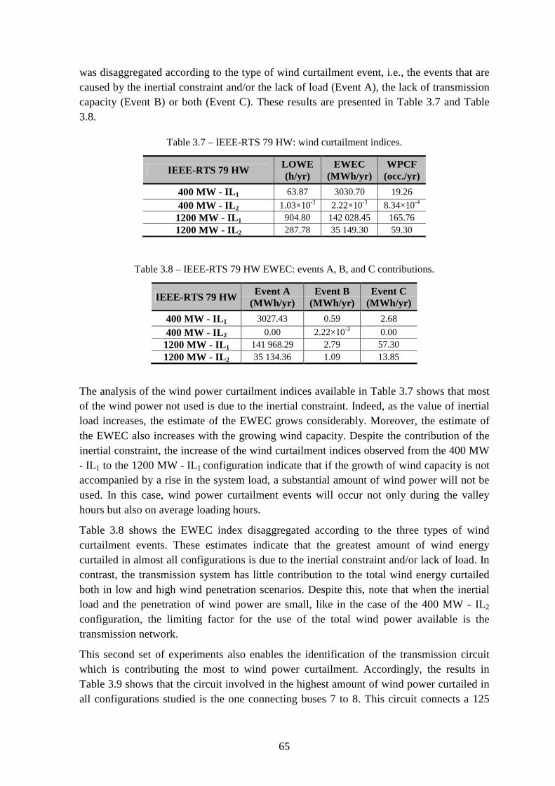
65

was disaggregated according to the type of wind curtailment event, i.e., the events that are caused by the inertial constraint and/or the lack of load (Event A), the lack of transmission capacity (Event B) or both (Event C). These results are presented in Table 3.7 and Table 3.8.

Table 3.7 – IEEE-RTS 79 HW: wind curtailment indices.

IEEE-RTS 79 HW LOWE (h/yr)

EWEC (MWh/yr)

WPCF (occ./yr)

400 MW - IL 1 63.87 3030.70 19.26

400 MW - IL 2 1.03×10-3 2.22×10-3 8.34×10-4 1200 MW - IL1 904.80 142 028.45 165.76 1200 MW - IL2 287.78 35 149.30 59.30

Table 3.8 – IEEE-RTS 79 HW EWEC: events A, B, and C contributions.

IEEE-RTS 79 HW Event A (MWh/yr)

Event B (MWh/yr)

Event C (MWh/yr)

400 MW - IL 1 3027.43 0.59 2.68

400 MW - IL 2 0.00 2.22×10-3 0.00 1200 MW - IL1 141 968.29 2.79 57.30 1200 MW - IL2 35 134.36 1.09 13.85

The analysis of the wind power curtailment indices available in Table 3.7 shows that most of the wind power not used is due to the inertial constraint. Indeed, as the value of inertial load increases, the estimate of the EWEC grows considerably. Moreover, the estimate of the EWEC also increases with the growing wind capacity. Despite the contribution of the inertial constraint, the increase of the wind curtailment indices observed from the 400 MW - IL1 to the 1200 MW - IL1 configuration indicate that if the growth of wind capacity is not accompanied by a rise in the system load, a substantial amount of wind power will not be used. In this case, wind power curtailment events will occur not only during the valley hours but also on average loading hours.

Table 3.8 shows the EWEC index disaggregated according to the three types of wind curtailment events. These estimates indicate that the greatest amount of wind energy curtailed in almost all configurations is due to the inertial constraint and/or lack of load. In contrast, the transmission system has little contribution to the total wind energy curtailed both in low and high wind penetration scenarios. Despite this, note that when the inertial load and the penetration of wind power are small, like in the case of the 400 MW - IL2

configuration, the limiting factor for the use of the total wind power available is the transmission network.

This second set of experiments also enables the identification of the transmission circuit which is contributing the most to wind power curtailment. Accordingly, the results in Table 3.9 shows that the circuit involved in the highest amount of wind power curtailed in all configurations studied is the one connecting buses 7 to 8. This circuit connects a 125

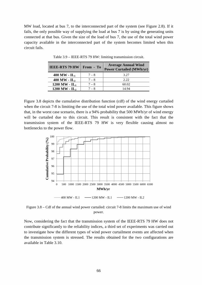
66

MW load, located at bus 7, to the interconnected part of the system (see Figure 2.8). If it fails, the only possible way of supplying the load at bus 7 is by using the generating units connected at that bus. Given the size of the load of bus 7, the use of the total wind power capacity available in the interconnected part of the system becomes limited when this circuit fails.

Table 3.9 – IEEE-RTS 79 HW: limiting transmission circuit.

IEEE-RTS 79 HW From - To Average Annual Wind

Power Curtailed (MWh/yr)

400 MW - IL 1 7 – 8 3.27

400 MW - IL 2 7 – 8 2.22 1200 MW - IL1 7 – 8 60.02 1200 MW - IL2 7 – 8 14.94

Figure 3.8 depicts the cumulative distribution function (cdf) of the wind energy curtailed when the circuit 7-8 is limiting the use of the total wind power available. This figure shows that, in the worst case scenario, there is a 94% probability that 500 MWh/yr of wind energy will be curtailed due to this circuit. This result is consistent with the fact that the transmission system of the IEEE-RTS 79 HW is very flexible causing almost no bottlenecks to the power flow.

Figure 3.8 – Cdf of the annual wind power curtailed: circuit 7-8 limits the maximum use of wind power.

Now, considering the fact that the transmission system of the IEEE-RTS 79 HW does not contribute significantly to the reliability indices, a third set of experiments was carried out to investigate how the different types of wind power curtailment events are affected when the transmission system is stressed. The results obtained for the two configurations are available in Table 3.10.

94

95

96

97

98

99

100

0 500 1000 1500 2000 2500 3000 3500 4000 4500 5000 5500 6000 6500

Cum

ulat

ive

Pro

babi

lity

(%)

MWh/yr

400 MW - IL1 1200 MW - IL1 1200 MW - IL2

67

Table 3.10 – IEEE-RTS 79 HW 1.5: composite system adequacy indices.

IEEE-RTS 79 HW LOLE (h/yr)

EENS (MWh/yr)

LOLF (occ./yr)

600 MW - IL 2 17.23 3358.52 3.52

1800 MW - IL2 7.56 1353.25 1.61

The comparison of the estimates of the reliability indices in Table 3.4 with the equivalent ones for the 400 MW and 1200 MW configurations in Table 3.10, one observes that the increase of the generating capacity and the system load by factor of 1.5 has deteriorated considerably the adequacy of the composite system. For instance, note that for the 400 MW and 600 MW configurations, the EENS has increased from 1353.25 MWh/yr to 3358.52 MWh/yr. This performance decline indicates that the transmission system of the 600 MW - IL2 and 1800 MW - IL2 configurations imposes severe constrains to the power flow.

The results of the third set of experiments regarding wind power curtailment events are summarized in Table 3.11, Table 3.12, and Table 3.13. Table 3.11 shows the wind power curtailment indices for the two simulated configurations of the IEEE-RTS 79 HW. Like in the case of the reliability indices, these results can be compared with those in Table 3.7 since the 600 MW - IL2 and the 1800 MW - IL2 configurations result from the multiplication of the generating capacity and the system load of the 400 MW - IL2 and the 1200 MW - IL2 configurations by a factor of 1.5.

Table 3.11 – IEEE-RTS 79 HW 1.5: wind curtailment indices.

IEEE-RTS 79 HW LOWE (h/yr)

EWEC (MWh/yr)

WPCF (occ./yr)

600 MW - IL 2 3.53×10-3 0.12 3.89×10-3

1800 MW - IL2 289.79 53 089.22 59.73

Table 3.12 – IEEE-RTS 79 HW 1.5 EWEC: events A, B, and C contributions.

IEEE-RTS 79 HW Event A (MWh/yr)

Event B (MWh/yr)

Event C (MWh/yr)

600 MW - IL 2 0.00 0.12 0.00 1800 MW - IL2 53 029.43 15.93 43.87

Table 3.13 – IEEE-RTS 79 HW 1.5 EWEC: limiting transmission circuit.

IEEE-RTS 79 HW From - To Average Annual Wind Power Curtailed (MWh/yr)

600 MW - IL 2 16 - 19 0.29

1800 MW - IL2 16 - 19 36.09

68

The analysis of the results in Table 3.11 with the ones reported in Table 3.7 shows that the probability and frequency of wind curtailment events are not much affected when the transmission system is stressed. As a matter of fact, the comparison of the results of the 1200 MW - IL2 with those of the 1800 MW - IL2, reveals that the EWEC has increased by a factor of 1.51, almost the same factor by which the generating capacity and the load were increased. Hence, even in a congested transmission system, loading limits and/or forced outages of transmission circuits may not significantly affect the average wind power curtailed as compared to the inertial constraint.

The conclusion of the last paragraph is corroborated by the comparison of the results of the 1200 MW - IL2 available in Table 3.8 with the equivalent ones obtained for the 1800 MW - IL2 configuration reported in Table 3.12. This comparison shows that the expected wind power curtailed associated with Event A has grown by a factor of 1.5, whereas the increase in the case of Event B is 14.6, and 3.17 in the case of Event C. Despite the dissimilar growth, which is more pronounced in the events involving transmission circuits, the greatest share of wind power curtailed is still associated with Event A. Once again, the conclusion that can be drawn is that the transmission system may not be the main obstacle to the maximum integration of wind power even when it is stressed.

Finally, consider the results in Table 3.13. When the transmission system becomes stressed, the circuit responsible for the highest amount of wind power curtailed is the one connecting bus 16 to 19, which is different from the circuit when the transmission system was not stressed (see Table 3.9). As a matter of fact, the bottleneck inside the 230 kV area has become more relevant to wind curtailment events than the failure of the radial circuit connecting bus 7 to the interconnected part of the IEEE-RTS 79 HW. Form this result one can conclude that a different circuit may arise as the one that limits the use of the total wind power available the most depending on the loading level of the transmission system.

3.8. Conclusions

This chapter proposed the use of the sequential MCS method developed within the scope of this dissertation to investigate the causes that limit the use of the total wind power available and how much wind energy is not used due to these restrictions. This analysis not only confirmed the full potential and the flexibility of the sequential MCS method developed but also provided new insights on a timely power system adequacy assessment problem.

The chapter started with an overview of the adequacy studies in the literature that include wind power. This literature review showed that the adequacy problems addressed in this chapter are original. Moreover, the review of the models of the WFs used in the long-term adequacy assessment of power systems uncovered their respective benefits and drawbacks.

Wind power curtailment events in a planning perspective were also investigated in this chapter. Accordingly, the following categorization for the events that can limit the use of the total wind power available was proposed:

69

• Event A: wind power curtailment due to the enforcement of the inertial constraint and/or load deficit;

• Event B: wind power curtailment due to transmission circuit failures and/or capacity limits;

• Event C: wind power curtailment due to the simultaneous occurrence of events A and B.

The inertial constraint, which is mentioned in Event A, is a simple model that accounts for the generating units dispatch preferences of system operators when a great share of the generating capacity is intermittent. Basically, this model assumes that a fixed amount of load, named inertial load, has always to be supplied by a given set of generating units regardless of the hourly load variation.

Similarly to the traditional reliability indices, this chapter demonstrated how to detect and estimate indices for the wind power curtailment events. For this purpose, a simple algorithm was proposed to detect whether wind curtailment events are due to the enforcement of the inertial constraint and/or load deficit, the failure and/or capacity limits of transmission circuits or the simultaneous occurrence of both of these events. Furthermore, it was shown how the circuits involved in the wind curtailment events can be identified using the sensitivity coefficients of the equality constraints of the DC OPF procedure. This identification enables the assessment of useful statistics, like the cdf of the wind power curtailed due to transmission capacity limitations.

The impact of the wind and thermal technologies on the adequacy of the composite system was also investigated in this chapter. The experiments carried out showed that, if the EAME performance measure is used instead of the installed capacity of the units, wind power is able to provide a better LOLE and EENS than a thermal unit. To this observation contributes the fact that, contrarily to a large thermal unit, WFs are aggregations of several small generating units. Moreover, since the wind capacity is dispersed throughout the transmission network and not concentrated at a single node, the average load curtailed due to the lack of transmission capacity is decreased. However, the same conclusion is not valid for the case of the LOLF. In the case of this index, wind intermittency can make the occurrence of loss of load events more frequent. From what has been said, the outcome of the traditional comparison between wind and thermal technologies is strongly dependent on the performance criterion adopted.

The wind power curtailment events under a strategy of maximum use of wind power were also analyzed. It was shown for the cases studied that the loading level of the transmission network does not limit the use of wind power as severely as the inertial constraint. Moreover, it was observed that the circuit that limits the use of wind power the most depends on the loading of the transmission network.

The analysis of the wind power curtailment events also proved that the growth of the inertial load implies considerable amounts of wind energy not used. Even if the inertial load remains constant, a huge quantity of wind power will be curtailed if the system load is insufficient to accommodate the additional wind capacity

70

As a concluding remark, there may be other systems where the transmission circuits play a more important role on wind curtailment events. Surely, the approach proposed in this chapter will capture these events and will provide system planners with valuable information to adequately cope with them.

71

Chapter 4

Sequential Monte Carlo Simulation using the Cross-Entropy Method and Importance Sampling

4.1. Introduction

This dissertation has shown that the sequential MCS method can synthetically create sequences of events and their respective duration. For this reason, this method can easily include all chronological aspects of power systems into the simulation, like correlated chronological load models, time-dependent load loss cost, programmed maintenance, and non-Markovian representations for the unavailability of the system components. In addition, this is the only method capable of providing the probability distribution of the reliability indices.

Despite these advantages, this method is time-inefficient [5], [9], [71]. The reason for this shortcoming lies in the sequential process for sampling system states. According to this process, a new system state is obtained from the preceding one by sampling a new state for only one system component [5], [9], [71]. Therefore, the difference between two system states sampled consecutively is the state of one and only one component. On top of that, the number of samples needed to assure accurate estimates of the reliability indices depends on the level of accuracy desired for the estimates [5]. In other words, the time-efficiency of the sequential MCS method is strongly affected by how reliable the system is.

A way to make the sequential MCS method more time-efficient is to use VRTs. In simple terms, these techniques aim to decrease the variance of the estimators of the reliability indices without affecting their expected value [5], [7–10], [12], [22–25], [39], [142], [143]. For this reason, VRTs can reduce the number of samples needed for obtaining estimates of the indices with the desired level of accuracy, or, in simple terms, increase the accuracy of the estimates for the required number of samples. Since simulation is normally stopped when a given level of accuracy is obtained, a smaller amount of samples results in a speed up over the crude sequential MCS method.

A considerable number of VRT such as Antithetic Variables (AV) [12], [24], [143], CV [22], [23], [143], SS [24], Latin Hypercube Sampling (LHS) [142], IS [7], [8], [39], and combinations of these VRT [72] have been used to speed up the process of estimating the

72

reliability indices through MCS methods. Recent work has showed that the sampling efficiency of MCS methods can be greatly improved by using IS [7], [8], [141]. This VRT uses a sampling distribution different from the original one to favor the appearance of the “most important” system states. In other words, the purpose of IS is to sample the states that contribute to the estimators of the reliability indices the most while keeping their underlying variance at minimum levels. Until recently, the selection of a “good” IS distribution was deemed as a difficult task [10]. This problem has been overcome by the CE method [26]. This method is able to provide a good approximation to the optimal IS distribution through a relatively simple and adaptive algorithm [26]. Thus, the combination of the CE method with the IS technique forms a simple and straightforward methodology to improve the sampling efficiency of the sequential MCS method and, as a result, its time-efficiency. Taking this into account, this chapter investigates the CE method and proposes several experiments to demonstrate the actual savings in time when this method is combined with IS and the sequential MCS method.

4.2. Convergence Characteristics of Monte Carlo Simulation Methods

Consider a vector of d-dimensional independent random variables X = (X1, …, Xd), that follows a given probability mass function f(X). A realization x of X can be seen as a system state. The expected value of a scalar function H of X is

[ ] ∑∈

==Xx

xxX )()()( fHHE fθ . (4.1)

If N samples of X are drawn from f(X), θ can be estimated using the unbiased estimator of the sample mean

( )∑=

=N

i

iHN 1

1~xθ . (4.2)

The variance of the estimator represented by (4.2) is

[ ]N

Varf

2~ σθ = (4.3)

where σ2 = Varf(θ) is the variance of H(X). Since neither θ nor σ2 is known at the beginning of the simulation, the variance of θ can be estimated as

( )( )∑=

−−

=N

i

iHN

s1

22 ~

1

1 θx . (4.4)

It has been shown that E[s2] = σ2 [10]. Normally, the coefficient of variation of θ~

[ ]

θθβ ~

~Var= , (4.5)

73

is used to gauge the convergence of MCS methods [5]. This coefficient is a normalized measure of the dispersion of probability distributions. Hence, the lower its value, the better is the accuracy of the estimate of θ.

Consider now that the function H(X), which is a scalar function of d random variables, follows a Bernoulli distribution [81]. According to this, Ef[H(X)] = p and Varf[H(X)] = p × (1 − p). Bearing this in mind, the number of samples NS required to obtain an estimate for p with a given level of accuracy βS is

2

1

S

Sp

pN

β×−

= (4.6)

If p << 1, which is the case of the loss of load probability of typical power systems, one has

2

1

S

Sp

Nβ×

= . (4.7)

This last equation expresses some convergence characteristics of the MCS methods. First of all, the number of samples required to assure that the estimate has a given level of accuracy depend on the reciprocal of the magnitude of the parameter being estimated. Hence, the lower the value of p, the greater is the number of samples needed. In addition, this equation shows that the number of samples does not depend on the size or complexity of the model of the system under simulation. This characteristic explains why MCS methods are preferably used to assess the adequacy of large-scale and complex power systems. Finally, the number of samples needed is considerably affected by the value of the coefficient of variation βS. For instance, if βS is reduced by a factor of two, the number of samples required rises fourfold.

The only way to circumvent this problem is to use VRTs. These techniques propose new estimators so that the number of samples NS required to obtain an estimate for p with the level of accuracy βS is lower than if the crude estimator, which is expressed by (4.2), is used.

Note that the previous equations can be directly applied for the case of the non-sequential MCS method. Nonetheless, the same reasoning can be applied for the sequential MCS method by assuming that a sample is sequence of random vectors, like the sequence {x1, …, xS} S ∈ ℕ, and not an individual vector x. Naturally, the scalar function H, which can also follow a Bernoulli distribution, has to be modified to evaluate these sequences {x1, …, xS} instead of x.

4.3. Variance Reduction Techniques

The number of samples required by the non-sequential and sequential MCS methods can be reduced using VRT. These techniques rely on information about the model of the system under simulation gathered a priori. Generally, the more is known about the model,

74

the more effective is the variance reduction. One way of acquiring this information is through a simulation of a simplified version of the model. The outcome of this first preliminary simulation can be used subsequently by a VRT to reduce the variance of the estimators used in the simulation of the complete model of the system.

Some VRTs, such as AV, CV, Conditional Monte Carlo (CMC), and SS take advantage of possible correlations between random variables [10]. Conversely, IS uses a new sampling distribution so that the events more important to the parameter under estimation are sampled more often [10]. This last VRT can greatly reduce the variance of the estimators, which is particularly important when rare-event probabilities are being estimated. The following sections briefly present IS and other VRTs available in the literature.

4.3.1. Antithetic Variables

Consider the random variable X. Assume also that θ = E[X]. The AV technique consists of using a pair of real-valued random variables (X, X*), which have the same probability distribution but are not independent [10]. According to this VRT, the following estimator can be used to obtain an estimate for θ

( )∑=

∗+=2/

1

1~ N

i

ii xxN

θ (4.8)

where N is the number of samples. The variance of this estimator is

[ ] [ ] [ ] [ ]( )∗∗ ×++= XXCovXVarXVarN

NVar ,2

2~2

θ . (4.9)

This last equation shows that the variance of the antithetic estimator can be reduced if the antithetic pair of random variables has negative correlation. Therefore, the variance reduction is greatly dependent on a good choice of the antithetic pair (X, X*).

4.3.2. Control Variables

The CV [10] is a well-known VRT and have many application in power systems adequacy assessment. Once again, consider the expectation θ = E[X]. This VRT consist on using a control variable C for X, whose expectation l = E[C] is known, in the following estimator

( )( )∑=

−×−=N

i

ii lcxN 1

1~ αθ (4.10)

where N is the number of samples and α is a scalar parameter called the linear control variable. The variance of the estimator represented by (4.20) is

[ ] [ ] [ ] [ ]CVarCXCovXVarVar ×+××−= 2,2~ ααθ . (4.11)

75

The optimal value of α that minimizes the variance of this estimator is obtained by solving the quadratic equation represented by (4.11). This process [10] yields

[ ]

[ ]CVar

CXCov ,=∗α . (4.12)

By substituting (4.12) in (4.11), one obtains

[ ] [ ]( ) [ ]XVarCXCorrVar ×−=∗2,1

~αθ . (4.13)

This last equation shows that the higher the reduction in variance increases with the correlation between X and C. In practical applications, neither the correlation between X and C nor the variance of X is known before the simulation of the model. Therefore, the linear control variable must be selected rather than calculated.

4.3.3. Conditional Monte Carlo

Consider, once again, the expectation θ = E[X]. Suppose also that there is a random vector Z such that the conditional expectation E[X|Z = z] can be computed analytically and in a fast way. Moreover, assume that drawing samples from Z is relatively easy to do. Taking this into account, the CMC [10] estimator for θ = E[X] = E[E[X|Z]] [10] is written as

[ ]∑=

=N

i

iXEN 1

|1~

Zθ . (4.14)

where N is the number of samples.

According to the assumptions stated previously, the variance of X can be expressed as

[ ] [ ][ ] [ ][ ]ZZ || XEVarXVarEXVar += . (4.15)

Since E[Var[X|Z]] is a non-negative value, this last equation shows that Var[E[X|Z]] ≤ Var[X]. For that reason, the estimator of CMC will have, in the worst case, a variance equal to the equivalent estimator of crude MCS. Unlike the case of AV and CV, this technique assures that there will always be variance reduction.

4.3.4. Stratified Sampling

SS [10] is closely related to the CMC. Suppose that the random variable X, whose expectation is θ = E[X], can be generated using an auxiliary random variable Z via the composition method [10], as follows:

Step a) Generate the random variable Z according to P({ Z = i}) = pi, i = 1, …, m;

Step b) Given {Z = i}, generate X.

Taking this into account, the following expression can be used to calculate the expectation

76

[ ][ ] [ ]iZXEpZXEEm

i

i === ∑=

||1

θ (4.16)

where the random variable Z takes values in {1, …, m} with known probabilities {pi, i = 1, …, m}.

The events {Z = i} can be viewed as partitions of the sample space, i.e., disjoint strata, hence the name SS. Usually, the number of strata, m, must be selected and depends on the model being simulated.

Under these assumptions, the SS estimator of θ is written as

×= ∑∑

==

iN

j

iji

m

i

i XN

p11

1~θ (4.17)

where Xij is jth of Ni observations from the conditional distribution of X given {Z = i}. Accordingly, the variance of this estimator is expressed as

[ ] [ ]∑

=

=×=

m

i i

i

N

iZXVarpVar

1

2 |~θ . (4.18)

where Var[X|Z = i] is the variance of X within the i th stratum.

If the sample size Ni of each stratum i is chosen proportionally to pi, i.e., Ni = pi × N, this VRT is called Proportional Stratified Sampling. Conversely, if pi = 1 / m and Ni = N / m, the technique is named Systematic Stratified Sampling. This last technique is very useful when dealing with uniform random variables.

As a final remark, the SS technique assumes that it is easy to sample from the conditional distribution of X given Z, which may not be the case for high-dimensional sample spaces.

4.3.5. Latin Hypercube Sampling

LHS [10] is an efficient VRT that circumvents the difficulties of SS for high-dimensional sample spaces. If SS is used for a space composed of d-dimensional uniform random variables, whose N / m is the number samples per stratum, one would have to draw (N / m)d samples to expect that at least one sample is drawn from every stratum. To circumvent this problem, LHS proposes the stratification of the probability distributions of the random variables rather than the entire sample space.

The process of drawing a sample according to LHS is not trivial. To begin with, consider a vector of d-dimensional independent uniform random variables X = (X1, …, Xd) and a scalar function H(X). Fixing m as the number of strata per random variable, which must be equal for all variables, and N as the total number of samples, generate n = N / m independent samples {Ui

1, …, Uid}, Ui = (ui1, …, uim), ui ~ U(0, 1), i = 1, …, n.

Additionally, generate n independent permutations {πi1, …, πi

d}, πi = (1, …, m), i = 1, …, n. Accordingly, m samples of X are generated in each iteration i of the LHS technique. Hence, the sample X ij, j = 1, …, m, is

77

−+−+=

m

u

m

u dij

dijijij

ij

1,...,

1 11 ππX . (4.19)

Finally, the LHS estimator of θ = E[H(X)] is

( )∑ ∑= =

=

n

i

m

j

ijHmn 1 1

11~Xθ (4.20)

4.3.6. Importance Sampling

Consider a vector of d-dimensional independent random variables X = (X1, …, Xd) and a scalar function H of X. As previously mentioned, the IS [10] technique uses a new sampling distribution g(X), which has different parameters from f(X), to sample the events that contribute to the parameter under estimation θ = Ef[H(X)] more often.

The samples drawn from the distribution g(X) are biased. Hence, the IS estimator of θ = Ef[H(X)] must be corrected using a weighting factor, as

( ) ( )∑=

=N

i

ii WHN 1

1~xxθ (4.21)

where W(xi) = f(xi) / g(xi) is called the likelihood ratio. This ratio represents the correction that must be made since samples are drawn from g(X) instead from f(X).

According to (4.21), the minimum variance of the IS estimator is obtained by solving

( ) ( )( )

X

XX

g

fHVargmin (4.22)

Assuming that H(X) ≥ 0, the optimal sampling distribution g*(X) is [10]

( ) ( ) ( )θ

XXX

fHg =* (4.23)

and

[ ] [ ] 0~

** == θθ gg VarVar (4.24)

Hence, the optimal sampling distribution is only available if the value of the θ = E[H(X)] is known a priori, which is precisely what is being estimated [10].

4.4. The Cross-Entropy Method for Rare-event Simulation

The previous section showed that the efficiency of the IS technique depends on the quality of the IS distribution g(X). Hence, this distribution must be at least “close” to the optimal IS distribution g*(X) to achieve a substantial reduction in variance.

78

To obtain g(X), the variance of the IS estimator can be minimized. However, the development of efficient computer routines based on this concept is extremely difficult since complex stochastic optimization may be involved [10]. As an alternative, the CE method [26] can be used to systematically obtain g(X). Moreover, this method can be applied to combinatorial optimization problems [26]. However, the focus on this dissertation is to use it to estimate expectations such as θ = E[H(X)]. In this last type of application, the CE method has proved to be an effective way to estimate rare-event probabilities, which are typically characterized by probabilities less than or equal to 1×10-5.

To begin with the demonstration of the CE method, assume that g(X) is a probability distribution belonging to the family of densities f(X; v) where v is a vector of reference parameters. Likewise, f(X) can be rewritten as f(X; u), where u is also a vector of reference parameters. The core of the CE method is the minimization of the Kullback-Leibler distance between g(X) and g*(X) [26]. This distance is defined as

( ) ( )( ) ( )( )

( ) ( ) ( ) ( )∫∫ −=

= ∗ xxxxxxX

XXX dggdgg

g

gE,ggD g lnlnln ***

** . (4.25)

The minimization of (4.25) is equivalent to

( ) ( )∫ xxx dgg lnmax * . (4.26)

By replacing g*(X) by (4.23), g(X) by f(X;v) and f(X) by f(X;u) in (4.26) one has

( ) ( ) ( ) ( )[ ] ( )∫ ⇔ vXXvx

uxx;lnmax;ln

;max fHEdxf

fHuvv θ

. (4.27)

Naturally, the optimal vector of parameters v* is the outcome of this optimization problem.

Assume now that IS can be used iteratively to use to solve (4.27). In the first iteration of this procedure, IS will use a new sampling function f(X; w) with different parameters from f(X; u) and f(X; v). Accordingly, (4.27) is rewritten as

( )[ ] ( )( )

( )vXwX

uXX ;ln

;

;max f

f

fHEwv . (4.28)

The respective optimal vector of reference parameters v* is

( )[ ] ( ) ( )vXuwXXv ;ln,;maxarg* fWHEwv= (4.29)

where W(X; w, u) = f(X; u) / f(X; w).

One way to solve (4.29) is to use the following stochastic program

( ) ( ) ( )∑=

∗ =N

i

iiiv fWHN 1

;ln,;1

maxarg~ vxuwxxv (4.30)

where N is the number samples drawn from f(X; w).

Taking advantage that (4.30) is often convex and differentiable with respect to v, one can obtain an analytical solution to v* rather than an estimate [10]. Moreover, if f(X; v) belongs

79

to the Natural Exponential Family [144], the entry j, j = 1, …, d, of vector v can be calculated via

( ) ( )

( ) ( )∑

∑

=

==N

i

ii

N

i

ijii

j

WH

xWHv

1

1

,;

,;

uwxx

uwxx (4.31)

This last equation [10] shows that it is possible to create a IS-based multi-level algorithm to improve iteratively the reference parameters vj, j = 1, …, d, until the optimal vector v*

for the target defined by θ = E[H(X)] is obtained.

For clarification purposes, assume that the expectation θ = E[H(X)] can be expressed as P(S(X) ≥ γ), i.e., the probability that the outcome of a scalar function S of X is greater than or equal to γ. In this case, the function H(X) = I{S(X) ≥ γ} can be used to detect when this event occurs. Thus, H(X) = 1 if S(X) ≥ γ and H(X) = 0 if S(X) < γ. Bearing this in mind, the CE method for rare-event simulation creates iteratively a sequence of reference parameters {vt, t ≥ 0} and a sequence of levels {γt, t ≥ 0} until γt ≥ γ. The level γt is selected at every iteration t using a pre-specified quantile (1 − ρ) × N of the distribution of S(X) over the N samples of xi, i = 1, … ,N, i.e., γt := S[(1 − ρ)N], S[1] < S[…] < S[N]. Conversely, the vector vt−1, which was obtained at the iteration t – 1, is used as the new vector of reference parameters of the IS distribution f(X; w), i.e., wt = vt−1. According to this, (4.32) can be rewritten to show how the parameters vt can be recursively calculated using IS as

{ } ( )

{ } ( )∑

∑

=≥

=≥

− =N

i

t-iS

N

i

ijt-iS

tj

WI

xWIv

t

t

11)(

11)(

1,

,;

,;

uvx

uvx

X

X

γ

γ

. (4.32)

4.5. Generating Capacity Adequacy Assessment using the Cross-Entropy Method and Importance Sampling

The CE method can be applied to the generating capacity adequacy assessment since the probability distribution of the unavailability of the generating units - the Bernoulli distribution - belongs to the Natural Exponential Family [144]. Taking advantage of this, the authors of [7], [8] proposed a CE optimization algorithm for generating capacity adequacy assessment, which follows the same basic steps for all MCS variants regardless of the type of representation of the system states.

The parameters optimized by the CE optimization algorithm are the unavailability u of the generating units. Thus, the vector u, which contains the unavailability of the generating units, is altered in an iterative way until the convergence criterion is verified [7], [8]. The outcome of this optimization process is a distorted vector of unavailability v. The term distortion in this case refers to a change in the value of u, for example, from 0.05 to 0.70.

80

In doing so, the unavailability of the generating units still follows a Bernoulli distribution, however, with a distorted unavailability v [7], [8].

Once the CE optimal parameters are obtained, the IS-based MCS variants, which have the flexibility necessary to represent time-varying loads, renewable power fluctuation, scheduled maintenance schemes, etc., can be run to estimate the usual reliability indices. It was shown that the CPU time required by these IS-based MCS variants is minimum when the peak load LMAX or a load value very close to it is used to gauge the CE optimization algorithm, i.e., when γ ≈ LMAX [40].

In the non-sequential MCS method, the sampling distribution f(X; u) is completely characterized by the unavailability the generating units. As a result, the optimal sampling distribution f(X; v) obtained with the CE optimization algorithm can be directly used by the IS-based non-sequential MCS method. In the sequential MCS method, however, system states are sampled using the failure and repair rates of the generating units, i.e., the sampling distribution is f(X; u, λ, µ). In this case, the distortion must be applied not only to u but also to the parameters λ and µ of the generating units [8].

Considering the two-state Markov model (see Figure 2.6), the optimal CE distorted unavailability v* of a generating unit is

( )∗∗∗∗ += µλλ /v (4.33)

where λ* and µ* are the distorted failure and repair rates, respectively. According to this last equation, there is an infinite set of possible combinations for the distorted failure and repair rates that result in the required unavailability v*. In order to maximize the expected number of failure events in a given period of time, the distortion is applied only to the failure rate without changing the repair rate [8]. Hence, µ* = µ. After the optimal CE distorted parameters λ* and µ* are obtained for all generating units, the IS-based sequential MCS method can be executed. Note that only the unavailability of the generating units is distorted. The other chronological characteristics of the system, like annual load, programmed maintenance, etc., are modeled in the usual way.

To avoid biased estimates of the reliability indices, the outcome of H must be compensated. It was demonstrated in [8] that the duration of a state x sampled by the IS-based sequential MCS method can be individually corrected using

( ) ( )( )vx

u xµλvµλux

;

;,,,; **

f

f,,W = . (4.34)

This is the same likelihood ratio used by the IS-based non-sequential MCS method. Hence, the correction of H in the sequential simulation only depends on u and v. On the other hand, the test function of some reliability indices, such as the LOLC, requires the correct representation of the whole cycle of interruptions. In this case, the compensation factor described by (4.34) cannot be applied to compensate a sequence of states. In other words, a sequence of states cannot be compensated by individually compensating each state of the sequence. In this case, the conditional probability approach must be used to compensate the sequence of states {x1, …, xS}, S ∈ ℕ [8]. Mathematically this is represented by

81

{ }( ) ( ) ( ) ( )( ) ( ) ( )1

*12

*1

11211 |...|;

|...|;,;

−

−= ×××

×××=SS

SSSnn

PPf

PPfW

xxxxvxxxxxux

vux (4.35)

where f(x1) is the probability of the first state of the sequence and P(xS|xS-1) is the conditional probability of the state xS of the sequence given that the previous state was xS−1. The superscript * represents identical probability calculations using the distorted parameters. Note that the last equation can be used to compensate the total duration of the whole interruption as well as the curtailed energy. As a result, other indices such as the LOLE, EENS, and LOLD can be estimated by compensating whole interruption sequences rather than compensating failure states individually. Moreover, the sequential MCS method allows the representation of maintenance schedules for the generating units under an hourly, monthly, or seasonal basis. The generating units that are undergoing maintenance are not accounted for in the calculation of the likelihood ratio. The contribution of these units is only considered before and after the maintenance period, when its behavior is represented by a Markovian process with distorted parameters [8].

4.5.1. The CE Optimization Algorithm for the Generating Capacity Adequacy Assessment

Some generating units have the same capacity c and unavailability u. If these units are iid, they can be aggregated into NC groups to save computational effort. Bearing this in mind, the vector X = (X1, …, XNC) can be used to represent a generating state where the random variable Xj represents the number of units of group j in the up state.

The Binomial distribution can be used to represent a group of NG generating units. The probability mass function of the j-th group, j = 1, …, NC, is

( ) ( )( )jjj xNGj

xj

j

jjjj uu

x

NGuNGxf −×−×

= 1,; (4.36)

The main lines of the CE optimization algorithm for generating capacity adequacy assessment are presented in the Pseudocode 1 (PC1) [7], [8], [40], [41]. For illustration purposes, the annualized LOLP index, i.e., the probability of system failure for the peak load, is used to gauge the distortion. However, any other reliability index can be used for that purpose.

Pseudocode 1: CE Optimization Algorithm for the Generating Capacity Adequacy Assessment

Set the sample size N, the multi-level parameter ρ, and the maximum number of iterations tMAX

Set the peak load LMAX as target for obtaining v

v0 = u; t = 0

82

Do

t := t + 1

Sample xi, i = 1, …, N, using vt-1, where xi is a vector of Binomial random variables and xij is the number of generating units of the group j in the up state

Evaluate S(xi) for all x1, …, xN, where S(xi) is the total generating capacity of the state xi, i.e., S(xi) = ∑xij × cj , j = 1, …, NC

Sort all S(xi) in descending order, i.e.,, S[1] ≥ S[2] ≥ S[3] ≥ S[4] ≥… ≥ S[N]

Set [ ]Nρt SL )1(ˆ

−= if this is greater than MAXL ; then set MAXt LL =ˆ

Calculate HLOLP(xi) using

( ) ( )( ) ki

kii

LS

LSif

ifH

ˆ

ˆ

1

0LOLP

<≥

=

x

xx (4.37)

Calculate Wi(xi; vt-1, u) using

( )( )

( )∏

∏

=

−−−

=

−

−

−

−=

NC

j

xNGjt

xjt

NC

j

xNGj

xj

tiiijjij

ijjij

vv

uu

W

1

,1,1

11

1

1

,; uvx (4.38)

Calculate vt,j using

( ) ( )

( ) ( )∑

∑

=

=−=N

i

t-iii

N

i

ijt-iii

jjt

WH

x;WH

NGv

11LOLP

11LOLP

,

,;

,1

1uvxx

uvxx (4.39)

While MAXt LL >ˆ and t ≤ tMAX

4.5.1.1. Exploring the CE Optimization Algorithm

In the first iteration of the CE method, v is equal to u. As a result, the likelihood ratio W(X; v0, u) = 1 for all N samples. Now, assume that X is a vector of Bernoulli random variables, whose entries represent the state of a single generating unit, i.e., NGj = 1. According to this, (4.39) is simplified as

∑

∑

=

=−=N

i

i

N

i

iji

j

H

xHv

1LOLP

1LOLP

)(

)(1

x

x (4.40)

where j = 1, …, TNG (total number of generating units). This last equation can be rewritten as

83

∑

∑

=

==−N

i

i

N

i

iji

j

HN

xHN

v

1LOLP

1LOLP

)(1

)(1

1x

x. (4.41)

Now, if N → ∞, then (4.39) is equivalent to

)]([

])([1

LOLP

LOLP

X

X

HE

XHEv

u

juj =− (4.42)

where Eu[HLOLP(X)] is the expected value of HLOLP(X) for the probability distribution f(X; u), which is the annualized LOLP index.

HLOLP(X), which is defined by (4.37), is function of a discrete vector of independent random variables and is itself a discrete random variable. Moreover, Xj is a Bernoulli random variable, which is equal to one if the generating unit j is in the up state, and 0, otherwise. Hence, E[HLOLP(X) × Xj] can be seen as the expected value of the product of two random variables.

Remembering that Xj is the j-th position of the vector X, the product of these discrete random variables can be expressed by the following variable

( ) ( )0

1

0LOLP

==

=

j

j

X

X

if

ifHY

XX . (4.43)

The conditional expectation [81] of Y(X) is

( )[ ] ( )[ ][ ]

[ ] ( ) [ ] ( )11|)(00|0

|

=×=+=×===

jjLOLPujju

juuu

XPXHEXPXE

XYEEYE

X

XX (4.44)

where Eu[HLOLP (X) | Xj = 1] is the Eu[HLOLP(X)] conditioned to the fact that the generating unit j is in the up state. Note that Xj is a deterministic variable in the calculation of this expectation, i.e., the value of Xj is constant and equal to 1.

By replacing (4.44) in (4.42) and taking into account that P(Xj = 1) = 1 − uj, the following equation is obtained

[ ] ( )j

u

juj u

HE

XHEv −

=−= 1

)]([

1|)(1

LOLP

LOLP

X

X (4.45)

This last equation shows that the parameter v of the generating unit j can be calculated in a single iteration of the CE optimization algorithm. The only requirement is to obtain Eu[HLOLP(X) | Xj = 1], which is the probability of system failure given that the generating unit j is always in the up state. Accordingly, (4.45) becomes

)1(LOLP

LOLP1 j

jj uv −−=

+

(4.46)

where LOLP is the probability of system failure considering LMAX and that LOLPj+ is the

same index assuming that the generating unit j can only reside in the up state.

84

According to (4.44), if LOLP and LOLPj+ are known, then the optimal v for the j-th

generating unit can be easily calculated. Other reliability indexes can be used in (4.46) to obtain similar distortions. For example, the EPNS and EPNSj

+ or the LOLF and LOLFj+

can be used to obtain specific distortions.

Now, since HLOLP(X) and Xj are discrete random variables, it is natural to define the conditional expectation of HLOLP(X) given Xj. Accordingly,

[ ] [ ][ ][ ] ( )[ ] ( )00|)(

11|)(

|)()(

LOLP

LOLP

LOLPLOLP

=×=+=×==

=

jju

jju

juu

XPXHE

XPXHE

XHEEHE

X

X

XX

. (4.47)

Knowing that P(Xj = 0) = uj, one has

jj

j uvLOLP

LOLP -

= (4.48)

where LOLPj- is the probability of system failure considering LMAX and assuming that, in

this case, the generating unit j can only reside in the down state. This last equation is equivalent to (4.46).

4.5.1.2. The Simplified CE Algorithm

To evaluate LOLP and LOLPj- for each generating unit j, a very efficient analytical method

based on discrete convolution is proposed. The use of discrete convolution for calculating generating capacity reliability indices consists of building an equivalent generation model for the system [11], [74]. More precisely, this process relies on the recursive use of two convolution equations for every generating unit at a time until all generators are accounted for. Details of this method can be found in [11], [74].

To help explain the discrete convolution process, consider a system composed of two generating units. Given the vectors of state capacities c, probabilities p, and incremental frequencies q of G1 = {cG1; pG1; qG1} and G2 = {cG2; pG2; qG2}, one wants to determine the same parameters for the generating system G = {cG; pG; qG}. The vectors of parameters p and q are sequences of impulses associated with the sequence of state capacities c. These

two sequences are equally spaced by a pre-defined rounding capacity increment ∆. To

obtain the parameters pG and qG, the following convolution (∗) equations are used

21 GGG ppp ∗= (4.49)

( ) ( )2121 GGGGG pqqpq ∗+∗= (4.50)

At the end of this recursive procedure, the parameters of the generating system G are expressed by the set G = {cG; pG; qG}. All convolution operations are performed through FFT techniques in order to improve the computational performance of convolution operations [42].

85

Now, note that PC1, which is the standard CE optimization process, is based on the non-sequential MCS method. In this algorithm, many samples are drawn and analyzed in order to obtain the optimal CE distortion for the unavailability of the generating units. Hence, the quality of the distortion obtained depends on the specified size of N (number of samples). In contrast, the simplified CE algorithm proposed can substitute the MCS-based optimization process by a simple analytical procedure. The main advantage of this approach is that the optimal distortion is no longer estimated, and thus, subjected to a convergence process, but rather calculated. Furthermore, the precision of the distortions

obtained by this method can be easily controlled with the specified rounding increment ∆.

The main lines of the simplified CE algorithm are presented in the Pseudocode 2 (PC2). Note that the annualized LOLP index, i.e., the LOLP index considering the peak load as the load level, is once again used to gauge the distortion. In order to save computational effort, the concept of groups of equal generation units is also adopted. Finally, all convolution operations are conducted using FFT.

Pseudocode 2: Simplified CE Algorithm for Generating Capacity Adequacy Assessment

Select the capacity rounding increment ∆

Set the peak load LMAX as target for obtaining v

NC = number of groups of independent and identically distributed generating units, i.e., with equal G and G-

Size a vector GC which contains the generating capacity models of the generation groups, a vector G which contains the model G of the different units.

GS = {0; 0; 0} ; tmpGS = {0; 0; 0}

For i = 1 to NC

NGi = number of generating units of the i-th group

Gi = {cGi; pGi; qGi} ; GCi = {0; 0; 0}

For j = 1 to NGi − 1

GCi := GCi + Gi

End For

GS := GS + ( GCi + Gi )

tmpGS := tmpGS + GCi

End For

Calculate LOLP considering GS and LMAX

For j = 1 to NC

GS- = tmpGS

86

For i = 1 to NC

If i ≠ j

GS- := GS- + ( GCi + Gi )

End If

End For

Calculate LOLPj- considering GS- and LMAX

Calculate vj according to (4.46)

End For

4.5.1.2.1. Numerical Example

To illustrate the simplicity of the proposed approach, consider a small generating system with 1 unit of 100 MW, 2 units of 250 MW, and 1 unit of 400 MW. Consider also that the failure and repair rates are the same for all units and equal to 9.22 failures/year and 175.20 repairs/year, respectively. Therefore, the unavailability of all generating units is equal to 0.05, i.e., u = [0.05, 0.05, 0.05]. The original IEEE-RTS 79 [91] load model is used with a peak load of 600 MW.

According to (4.46), only the values of LOLP and LOLPj- are needed to obtain the optimal

vector of distorted parameters v. These can be easily calculated by performing the discrete convolution operations described in PC2. Thus, LOLP = 9.50×10-3, which is the system failure probability considering only the peak load. LOLP1

- = 5.24×10-2, is the system failure probability considering both the peak load and that the 100 MW unit is always unavailable. Now, the optimal distorted unavailability for the 100 MW unit can be calculated as

.276.005.0109.50

1024.5

LOLP

LOLP3-

-2

11

1 =××==

−

uv (4.51)

The process is then repeated for the two remaining groups of generating units. Thus, LOLP2

- = 8.75×10-2, which is the system failure probability considering the peak load and that one unit of 250 MW is always in the down state. Similarly, LOLP3

- = 1.43×10-1 is the system failure probability considering the peak load and that the 400 MW unit is always unavailable. The values of v2 and v3 are then given by

513.005.0109.50

108.75

LOLP

LOLP3-

-2

22

2 =××==

−

uv (4.52)

750.005.0109.52

101.43

LOLP

LOLP3-

-1

33

3 =××==

−

uv (4.53)

and, therefore, v = [0.276, 0.513, 0.750]. This results are very close to v = [0.275, 0.518, 0.740], which was obtained using PC1 with N = 100 000 samples.

87

Now, the IS-based sequential MCS method can be run to assess the annual reliability indices considering all load levels and other chronological aspects such as capacity fluctuation and maintenance schemes. Actually, the annual reliability indices for this system are: LOLP = 3.22×10-3, EPNS = 2.78×10-1 MW, and LOLF = 3.31 occ./yr. Using u, i.e., the crude sequential MCS method, the simulation needed approximately 1.9×107 samples to converge to βMAX = 1% (for all indices). Conversely, by using v instead of u, only 4.2×105 samples were needed to reach the same accuracy, which clearly demonstrates the variance reduction properties of IS.

Finally, as stated in the previous section, EPNS and EPNSj- or LOLF and LOLFj

- could have been used in (4.51), (4.52), and (4.53) to obtain specific distortions for each reliability index.

4.5.1.3. Analysis of the Simplified CE Algorithm

To evaluate the accuracy and efficiency of the simplified CE algorithm, different generating systems were tested but only a few of them are fully reported and discussed.

Firstly, the proposed simplified CE-based method is used to determine the optimal IS distribution for the IEEE-RTS 79 [91] and the IEEE-RTS 96 [92]. Subsequently, the same set of tests is performed using two configurations of the Brazilian South-Southeastern (BSS) system [7], [11] planned for the 90’s: normal and reinforced configurations. All computations were performed in a MATLAB platform using an Intel Core i7-2600 with a 3.40 GHz processor.

4.5.1.3.1. Results for the IEEE-RTS 79

The IEEE-RTS 79 consists of 32 units totalizing 3405 MW of installed capacity. The load model consists of 8736 hourly levels with a peak load of 2850 MW. Table 4.1 shows the different generation groups that can be formed and also their respective capacities and unavailability.

Table 4.1 – IEEE-RTS 79 and IEEE-RTS 96 generating systems.

Group Unit Size (MW)

uj No. of Units

IEEE-RTS 79 IEEE-RTS 96 1 12 0.02 5 15 2 20 0.10 4 12 3 50 0.01 6 18 4 76 0.02 4 12 5 100 0.04 3 9 6 155 0.04 4 12 7 197 0.05 3 9 8 350 0.08 1 3 9 400 0.12 2 6

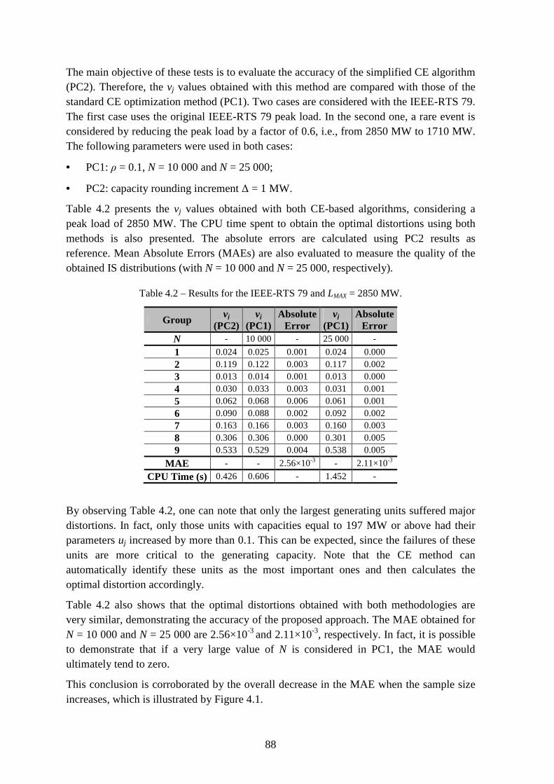
88

The main objective of these tests is to evaluate the accuracy of the simplified CE algorithm (PC2). Therefore, the vj values obtained with this method are compared with those of the standard CE optimization method (PC1). Two cases are considered with the IEEE-RTS 79. The first case uses the original IEEE-RTS 79 peak load. In the second one, a rare event is considered by reducing the peak load by a factor of 0.6, i.e., from 2850 MW to 1710 MW. The following parameters were used in both cases:

• PC1: ρ = 0.1, N = 10 000 and N = 25 000;

• PC2: capacity rounding increment ∆ = 1 MW.

Table 4.2 presents the vj values obtained with both CE-based algorithms, considering a peak load of 2850 MW. The CPU time spent to obtain the optimal distortions using both methods is also presented. The absolute errors are calculated using PC2 results as reference. Mean Absolute Errors (MAEs) are also evaluated to measure the quality of the obtained IS distributions (with N = 10 000 and N = 25 000, respectively).

Table 4.2 – Results for the IEEE-RTS 79 and LMAX = 2850 MW.

Group vj

(PC2) vj

(PC1) Absolute

Error vj

(PC1) Absolute

Error N - 10 000 - 25 000 -

1 0.024 0.025 0.001 0.024 0.000 2 0.119 0.122 0.003 0.117 0.002 3 0.013 0.014 0.001 0.013 0.000 4 0.030 0.033 0.003 0.031 0.001 5 0.062 0.068 0.006 0.061 0.001 6 0.090 0.088 0.002 0.092 0.002 7 0.163 0.166 0.003 0.160 0.003 8 0.306 0.306 0.000 0.301 0.005 9 0.533 0.529 0.004 0.538 0.005

MAE - - 2.56×10-3 - 2.11×10-3

CPU Time (s) 0.426 0.606 - 1.452 -

By observing Table 4.2, one can note that only the largest generating units suffered major distortions. In fact, only those units with capacities equal to 197 MW or above had their parameters uj increased by more than 0.1. This can be expected, since the failures of these units are more critical to the generating capacity. Note that the CE method can automatically identify these units as the most important ones and then calculates the optimal distortion accordingly.

Table 4.2 also shows that the optimal distortions obtained with both methodologies are very similar, demonstrating the accuracy of the proposed approach. The MAE obtained for N = 10 000 and N = 25 000 are 2.56×10-3 and 2.11×10-3, respectively. In fact, it is possible to demonstrate that if a very large value of N is considered in PC1, the MAE would ultimately tend to zero.

This conclusion is corroborated by the overall decrease in the MAE when the sample size increases, which is illustrated by Figure 4.1.

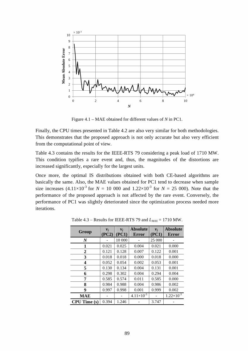
89

Figure 4.1 – MAE obtained for different values of N in PC1.

Finally, the CPU times presented in Table 4.2 are also very similar for both methodologies. This demonstrates that the proposed approach is not only accurate but also very efficient from the computational point of view.

Table 4.3 contains the results for the IEEE-RTS 79 considering a peak load of 1710 MW. This condition typifies a rare event and, thus, the magnitudes of the distortions are increased significantly, especially for the largest units.

Once more, the optimal IS distributions obtained with both CE-based algorithms are basically the same. Also, the MAE values obtained for PC1 tend to decrease when sample size increases (4.11×10-3 for N = 10 000 and 1.22×10-3 for N = 25 000). Note that the performance of the proposed approach is not affected by the rare event. Conversely, the performance of PC1 was slightly deteriorated since the optimization process needed more iterations.

Table 4.3 – Results for IEEE-RTS 79 and LMAX = 1710 MW.

Group vj

(PC2) vj

(PC1) Absolute

Error vj

(PC1) Absolute

Error N - 10 000 - 25 000 -

1 0.021 0.025 0.004 0.021 0.000 2 0.121 0.128 0.007 0.122 0.001 3 0.018 0.018 0.000 0.018 0.000 4 0.052 0.054 0.002 0.053 0.001 5 0.130 0.134 0.004 0.131 0.001 6 0.298 0.302 0.004 0.294 0.004 7 0.585 0.574 0.011 0.585 0.000 8 0.984 0.988 0.004 0.986 0.002 9 0.997 0.998 0.001 0.999 0.002

MAE - - 4.11×10-3 - 1.22×10-3

CPU Time (s) 0.394 1.246 - 3.747 -

0

1

2

3

4

5

6

7

8

9

10

0 2 4 6 8 10

Mea

n A

bsol

ute

Err

or

N

× 10-3

× 104

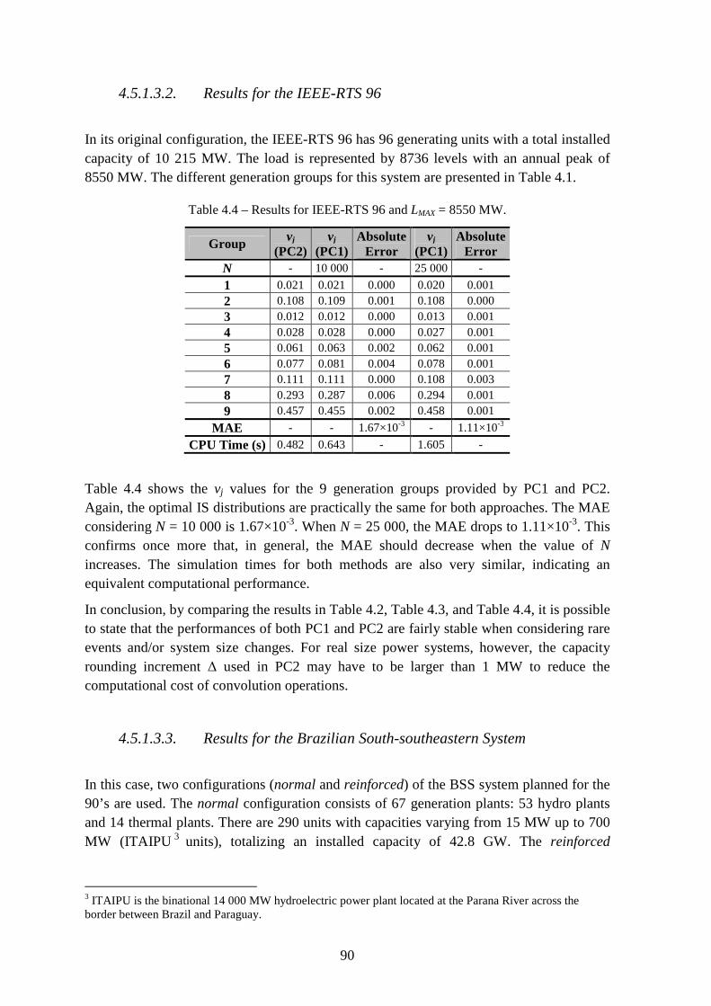
90

4.5.1.3.2. Results for the IEEE-RTS 96

In its original configuration, the IEEE-RTS 96 has 96 generating units with a total installed capacity of 10 215 MW. The load is represented by 8736 levels with an annual peak of 8550 MW. The different generation groups for this system are presented in Table 4.1.

Table 4.4 – Results for IEEE-RTS 96 and LMAX = 8550 MW.

Group vj (PC2)

vj (PC1)

Absolute Error

vj (PC1)

Absolute Error

N - 10 000 - 25 000 -

1 0.021 0.021 0.000 0.020 0.001 2 0.108 0.109 0.001 0.108 0.000 3 0.012 0.012 0.000 0.013 0.001 4 0.028 0.028 0.000 0.027 0.001 5 0.061 0.063 0.002 0.062 0.001 6 0.077 0.081 0.004 0.078 0.001 7 0.111 0.111 0.000 0.108 0.003 8 0.293 0.287 0.006 0.294 0.001 9 0.457 0.455 0.002 0.458 0.001

MAE - - 1.67×10-3 - 1.11×10-3

CPU Time (s) 0.482 0.643 - 1.605 -

Table 4.4 shows the vj values for the 9 generation groups provided by PC1 and PC2. Again, the optimal IS distributions are practically the same for both approaches. The MAE considering N = 10 000 is 1.67×10-3. When N = 25 000, the MAE drops to 1.11×10-3. This confirms once more that, in general, the MAE should decrease when the value of N increases. The simulation times for both methods are also very similar, indicating an equivalent computational performance.

In conclusion, by comparing the results in Table 4.2, Table 4.3, and Table 4.4, it is possible to state that the performances of both PC1 and PC2 are fairly stable when considering rare events and/or system size changes. For real size power systems, however, the capacity rounding increment ∆ used in PC2 may have to be larger than 1 MW to reduce the computational cost of convolution operations.

4.5.1.3.3. Results for the Brazilian South-southeastern System

In this case, two configurations (normal and reinforced) of the BSS system planned for the 90’s are used. The normal configuration consists of 67 generation plants: 53 hydro plants and 14 thermal plants. There are 290 units with capacities varying from 15 MW up to 700 MW (ITAIPU 3 units), totalizing an installed capacity of 42.8 GW. The reinforced

3 ITAIPU is the binational 14 000 MW hydroelectric power plant located at the Parana River across the border between Brazil and Paraguay.

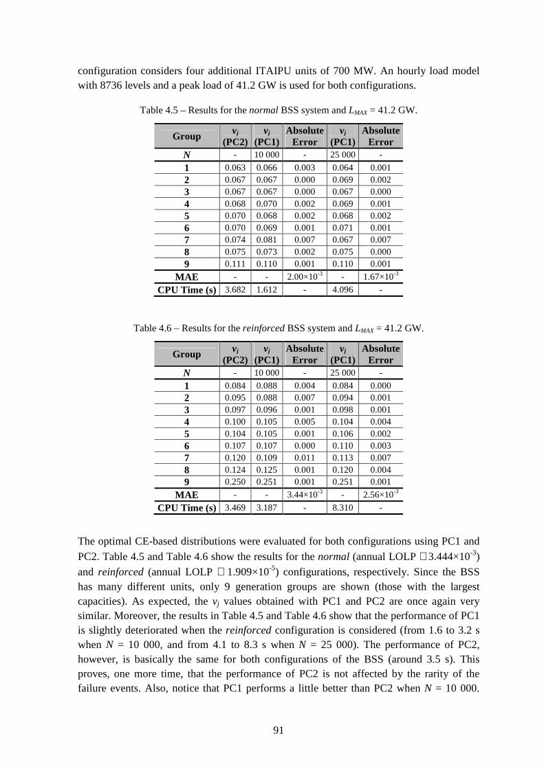
91

configuration considers four additional ITAIPU units of 700 MW. An hourly load model with 8736 levels and a peak load of 41.2 GW is used for both configurations.

Table 4.5 – Results for the normal BSS system and LMAX = 41.2 GW.

Group vj

(PC2) vj

(PC1) Absolute

Error vj

(PC1) Absolute

Error N - 10 000 - 25 000 -

1 0.063 0.066 0.003 0.064 0.001 2 0.067 0.067 0.000 0.069 0.002 3 0.067 0.067 0.000 0.067 0.000 4 0.068 0.070 0.002 0.069 0.001 5 0.070 0.068 0.002 0.068 0.002 6 0.070 0.069 0.001 0.071 0.001 7 0.074 0.081 0.007 0.067 0.007 8 0.075 0.073 0.002 0.075 0.000 9 0.111 0.110 0.001 0.110 0.001

MAE - - 2.00×10-3 - 1.67×10-3

CPU Time (s) 3.682 1.612 - 4.096 -

Table 4.6 – Results for the reinforced BSS system and LMAX = 41.2 GW.

Group vj (PC2)

vj (PC1)

Absolute Error

vj (PC1)

Absolute Error

N - 10 000 - 25 000 -

1 0.084 0.088 0.004 0.084 0.000 2 0.095 0.088 0.007 0.094 0.001 3 0.097 0.096 0.001 0.098 0.001 4 0.100 0.105 0.005 0.104 0.004 5 0.104 0.105 0.001 0.106 0.002 6 0.107 0.107 0.000 0.110 0.003 7 0.120 0.109 0.011 0.113 0.007 8 0.124 0.125 0.001 0.120 0.004 9 0.250 0.251 0.001 0.251 0.001

MAE - - 3.44×10-3 - 2.56×10-3

CPU Time (s) 3.469 3.187 - 8.310 -

The optimal CE-based distributions were evaluated for both configurations using PC1 and

PC2. Table 4.5 and Table 4.6 show the results for the normal (annual LOLP ≅ 3.444×10-3)

and reinforced (annual LOLP ≅ 1.909×10-5) configurations, respectively. Since the BSS has many different units, only 9 generation groups are shown (those with the largest capacities). As expected, the vj values obtained with PC1 and PC2 are once again very similar. Moreover, the results in Table 4.5 and Table 4.6 show that the performance of PC1 is slightly deteriorated when the reinforced configuration is considered (from 1.6 to 3.2 s when N = 10 000, and from 4.1 to 8.3 s when N = 25 000). The performance of PC2, however, is basically the same for both configurations of the BSS (around 3.5 s). This proves, one more time, that the performance of PC2 is not affected by the rarity of the failure events. Also, notice that PC1 performs a little better than PC2 when N = 10 000.

92

This was expected since the computational cost of convolution operations increases with the size of the systems. As such, the value of the capacity rounding increment ∆ should be chosen carefully, considering the tradeoff between accuracy and simulation time.

4.5.2. Analysis of the CE/IS Sequential MCS Method for the Generating Capacity Adequacy Assessment

The crude version (crude SMCS) and a CE/IS-based version of the sequential MCS method (CE/IS SMCS) was used to assess the adequacy of the generating capacity of two configurations of the IEEE-RTS 79. The first configuration uses the original peak load of the 2850 MW whereas the peak load of the second configuration is reduced by a factor of 0.6, i.e., from 2850 MW to 1710 MW. The parameters of the IS distribution were obtained using the simplified CE algorithm (PC2). The rounding increment adopted is ∆ = 1 MW. The distortions were gauged by the annualized LOLP index. The sequential MCS methods were stopped when the estimates of the annual reliability indexes had a β ≤ 5% or when 10 000 years of simulation had been simulated. The experiments were performed in a MATLAB platform using an Intel Core i7-2600 with a 3.40 GHz processor.

Table 4.7 – Results of PC2 and CE/IS SMCS (PC2) for the generating capacity of configurations of the IEEE-RTS 79 with LMAX = 2850 MW and LMAX =1710 MW.

IEEE-RTS 79 LMAX = 2850 MW LMAX = 1710 MW

PC2 Generation States Evaluated - - - -

CPU Time (min) - 7.10×10-3 - 6.57×10-3

Crude SMCS

CE/IS SMCS (PC2)

Crude SMCS

CE/IS SMCS (PC2)

SMCS

Generation States Evaluated 21 697 912 327 197 91 982 158 928 398 Years Simulated 2359 34 10 000 86 CPU Time (min) 47.5 0.76 193.78 2.11

LOLE (h/yr) 9.221 9.504 0.0 (100%) 5.991×10-6 EENS (MWh/yr) 1119.01 1190.31 0.0 (100%) 2.91×10-3 LOLF (occ./yr) 1.989 2.074 0.0 (100%) 2.024×10-5

Table 4.7 shows the estimates of the LOLE, EENS and LOLF indices for the two configurations of the IEEE-RTS 79 analyzed. These results are separated according to the version of the sequential MCS method used. For the simulations that reached 10 000 years, the coefficient of variation is displayed between brackets alongside the corresponding estimate of the index. This table also includes the number of states evaluated, the number of years simulated and the total time required by the respective version of the sequential MCS method.

The results in Table 4.7 show that, in the case of the 2850 MW peak load, the CE/IS SMCS version required only 1.5% of the states evaluated by the crude SMCS version. In other words, the crude SMCS has evaluated 66.3 times more states than the CE/IS SMCS. This less number of evaluations corresponds to a net speed up (the ratio between the CPU

93

time taken by the crude SMCS against the time taken by PC2 and the CE/IS SMCS) of 62.5.

Figure 4.2 – Estimate of the annual LOLE for the generating capacity of the IEEE-RTS 79 with LMAX = 2850 MW.

Figure 4.2 illustrates the reason for this remarkable speed up. This figure depicts the annual LOLE index for the generating capacity of the IEEE-RTS 79 configuration with LMAX = 2850 MW estimated by the two versions of the sequential MCS method. Note that the estimate of the LOLE index provided by CE/IS SMCS stabilizes much faster than the estimate of the crude SMCS. This means that the CE method can reduce considerably the variance of the IS estimator and, as a consequence, the number of simulated years, or, if one prefers, the number of state evaluations.

Moreover, the results in Table 4.7 for the configuration with a 1710 MW peak load demonstrate that the crude SMCS method was not able to provide accurate estimates for the reliability indices in 10 000 years of simulation. In contrast, the CE/IS SMCS needed only 2.11 minutes to evaluate the same configuration of the IEEE-RTS 79, or, in other words, 86 years of simulation. The true net speed up between the two versions of the sequential MCS method cannot be calculated for this configuration since, unlike the CE/IS SMCS, the crude SMCS was stopped before the estimates of the reliability indices had a β ≤ 5%. To guarantee a β ≤ 5%, the crude SMCS would need much more than 10 000 years of simulation. In any case, the results obtained allow calculating a pessimistic estimate for the net speed up. Bearing this in mind, the net speed up obtained is 91.84, which is very similar to the ratio between the number of states evaluated by the crude SMCS and the IS SMCS (this ratio is 99.08). In this case, the gain in time is inferior to the ratio between the states evaluated.

The overall conclusion from the results in Table 4.7 is that the number of evaluations required, and consequently the simulation time, can be dramatically reduced by using the IS technique with the sampling distribution optimized by the CE method. Moreover, these results showed that the speed up increases dramatically as the generating system becomes more reliable.

0

2

4

6

8

10

12

14

16

0 10 20 30 40 50 60 70 80 90 100

LOLE

(h/

yr)

Years Simulated

Crude SMCS CE/IS SMCS

94

Despite the remarkable gains, the CE/IS SMCS method has an important weakness. By using a distorted failure rate for the generating units while using the original repair rates and the chronological annual load, the true duration of system states is lost. In other words, since the loss of load events happen more frequently, the information required to build the annual probability distribution of the reliability indices becomes biased. Consider, for instance, the configuration of the IEEE-RTS 79 with 2850 MW peak load. The crude SMCS method has taken 2359 years to obtain estimates for the reliability indices with β ≤ 5%. During this time, there were some years that did not have a single loss of load event. On the contrary, the CE/IS SMCS method has required only 34 years of simulation to obtain similar estimates. Differently from the crude SMCS, all 34 years contained at least one loss of load event.

Figure 4.3 – Cdf of the annual LOLE for the generating capacity of the IEEE-RTS 79 with LMAX = 2850 MW.

Figure 4.3 highlights the different annual observations of the LOLE index provided by the crude and CE/IS versions of the sequential MCS method. In other words, this figure represents the cdf of the annual LOLE index. This figure confirms that, despite the remarkable convergence speed of the CE/IS SMCS, this method is not able, at least as it is, to provide the accurate annual probability distributions for the reliability indices.

4.5.2.1. Modeling the Generating Units with Time-dependent Capacity

PC1 and PC2 can provide the optimal CE distortions for the unavailability of the generating units that minimize the variance of the estimators of the subsequent CE/IS-based sequential MCS method. The two algorithms assume that the unavailability of the generating units follows the Bernoulli distribution. According to this distribution, the probability of finding the unit j in the up state is P(Xj = 1) = 1 − uj while the down state probability is uj. Supposing that the capacity of the unit j does not vary with time, the

0

10

20

30

40

50

60

70

80

90

100

0 20 40 60 80 100 120 140 160 180

Cum

ulat

ive

Pro

babi

lity

(%)

LOLE (h/yr)

Crude SMCS CE/IS SMCS

95

maximum capacity is available when the unit j is in the up state, i.e., when Xj = 1. As a matter of fact, the capacity of some units, like the hydro and WTGs, is time-dependent. This dependency is only accurately modeled using the sequential MCS method. Unfortunately, PC1 and PC2 are based on the state space representation, which makes impossible to sequentially follow annual series that represent the time-varying capacity of these generating units.

Due to the flexibility of the non-sequential MCS method, the time-dependency of the capacity of the generating units can be approximately incorporated in PC1 by randomly sampling realizations from the hydrological and wind annual series. Hence, each time a new state is sampled, one of the hydro or wind annual series can be selected according to its probabilities of occurrence. After that, the actual generating capacity of the hydro or WTGs is calculated by sampling an hourly realization from those series. Despite not being able to preserve the time-dependency of the generating units, this random sampling procedure can model the long-term capacity provided. For the sake of future referencing, this procedure is named Strategy A.

Since PC2 is based on convolution calculations, Strategy A cannot be used by this algorithm. To circumvent this problem, three approximate representations are proposed. The first one, which is named Strategy B, consists of calculating the average capacity provided by the generating units before running PC2. This procedure takes into account the hourly or monthly realizations of the hydrological and wind annual series as well as their respective probability of occurrence. The outcome of this procedure is used as an input of PC1, i.e., the average capacity is taken as the capacity of that these generating units have when they are in the up state. The second strategy, which is called Strategy C, is similar to Strategy B. In this case, the maximum capacity is obtained instead of the average capacity. The third and final strategy, which is the Strategy D, consists of using the minimum capacity. Note that strategies B, C and D do not require PC2 to be modified. In addition, they can be easily used by PC1.

Some generating units, such as WFs, have a smaller capacity factor than other units whose capacity varies with time. Moreover, since WFs are aggregations of several small WTGs, forced outages of the WTGs may not be as important to the power output of the WF as the wind availability. Bearing this in mind, one can assume that WTGs are always in the up state and they always produce a fixed amount of power in the calculation of the optimal CE distortions. This amount of power is the average capacity in the case of Strategy B, the maximum capacity in the case of Strategy C and the minimum capacity in the case of Strategy C. This assumption, which is used for the case of WFs, can be also adopted for other generating units that aggregate several small units and have low capacity factors.

4.5.2.1.1. Testing Strategies A, B, C and D

Strategies A, B, C and D were tested using the generating system of the IEEE-RTS 79 HW. This system, which has already been described in section 2.9.3.1, includes the time-

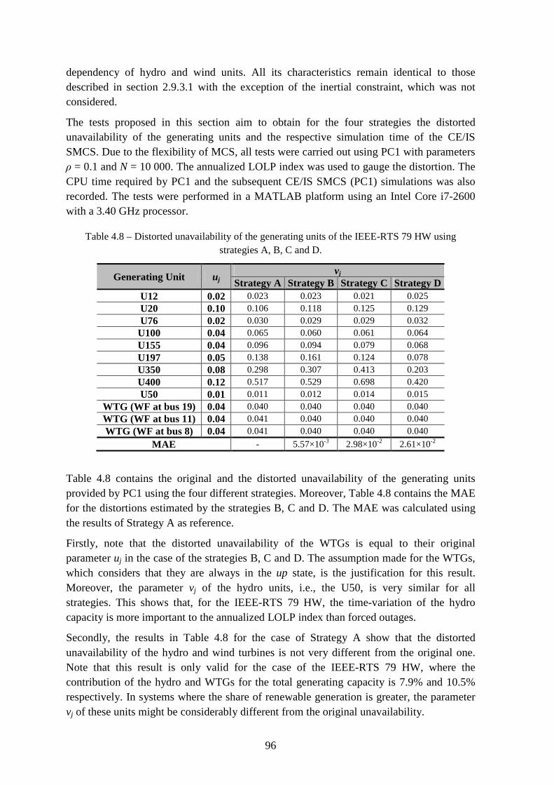
96

dependency of hydro and wind units. All its characteristics remain identical to those described in section 2.9.3.1 with the exception of the inertial constraint, which was not considered.

The tests proposed in this section aim to obtain for the four strategies the distorted unavailability of the generating units and the respective simulation time of the CE/IS SMCS. Due to the flexibility of MCS, all tests were carried out using PC1 with parameters ρ = 0.1 and N = 10 000. The annualized LOLP index was used to gauge the distortion. The CPU time required by PC1 and the subsequent CE/IS SMCS (PC1) simulations was also recorded. The tests were performed in a MATLAB platform using an Intel Core i7-2600 with a 3.40 GHz processor.

Table 4.8 – Distorted unavailability of the generating units of the IEEE-RTS 79 HW using strategies A, B, C and D.

Generating Unit uj vj

Strategy A Strategy B Strategy C Strategy D U12 0.02 0.023 0.023 0.021 0.025 U20 0.10 0.106 0.118 0.125 0.129 U76 0.02 0.030 0.029 0.029 0.032 U100 0.04 0.065 0.060 0.061 0.064 U155 0.04 0.096 0.094 0.079 0.068 U197 0.05 0.138 0.161 0.124 0.078 U350 0.08 0.298 0.307 0.413 0.203 U400 0.12 0.517 0.529 0.698 0.420 U50 0.01 0.011 0.012 0.014 0.015

WTG (WF at bus 19) 0.04 0.040 0.040 0.040 0.040 WTG (WF at bus 11) 0.04 0.041 0.040 0.040 0.040 WTG (WF at bus 8) 0.04 0.041 0.040 0.040 0.040

MAE - 5.57×10-3 2.98×10-2 2.61×10-2

Table 4.8 contains the original and the distorted unavailability of the generating units provided by PC1 using the four different strategies. Moreover, Table 4.8 contains the MAE for the distortions estimated by the strategies B, C and D. The MAE was calculated using the results of Strategy A as reference.

Firstly, note that the distorted unavailability of the WTGs is equal to their original parameter uj in the case of the strategies B, C and D. The assumption made for the WTGs, which considers that they are always in the up state, is the justification for this result. Moreover, the parameter vj of the hydro units, i.e., the U50, is very similar for all strategies. This shows that, for the IEEE-RTS 79 HW, the time-variation of the hydro capacity is more important to the annualized LOLP index than forced outages.

Secondly, the results in Table 4.8 for the case of Strategy A show that the distorted unavailability of the hydro and wind turbines is not very different from the original one. Note that this result is only valid for the case of the IEEE-RTS 79 HW, where the contribution of the hydro and WTGs for the total generating capacity is 7.9% and 10.5% respectively. In systems where the share of renewable generation is greater, the parameter vj of these units might be considerably different from the original unavailability.

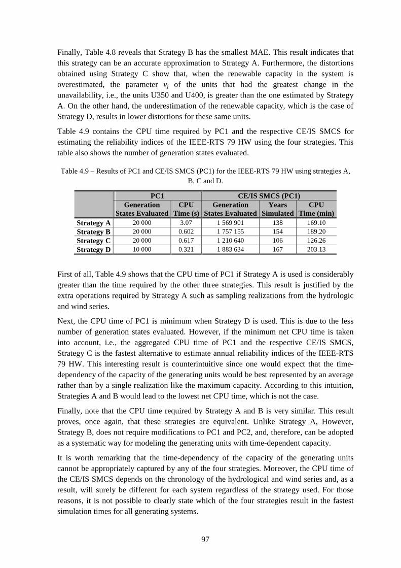
97

Finally, Table 4.8 reveals that Strategy B has the smallest MAE. This result indicates that this strategy can be an accurate approximation to Strategy A. Furthermore, the distortions obtained using Strategy C show that, when the renewable capacity in the system is overestimated, the parameter vj of the units that had the greatest change in the unavailability, i.e., the units U350 and U400, is greater than the one estimated by Strategy A. On the other hand, the underestimation of the renewable capacity, which is the case of Strategy D, results in lower distortions for these same units.

Table 4.9 contains the CPU time required by PC1 and the respective CE/IS SMCS for estimating the reliability indices of the IEEE-RTS 79 HW using the four strategies. This table also shows the number of generation states evaluated.

Table 4.9 – Results of PC1 and CE/IS SMCS (PC1) for the IEEE-RTS 79 HW using strategies A, B, C and D.

PC1 CE/IS SMCS (PC1) Generation

States Evaluated CPU

Time (s) Generation

States Evaluated Years

Simulated CPU

Time (min) Strategy A 20 000 3.07 1 569 901 138 169.10 Strategy B 20 000 0.602 1 757 155 154 189.20 Strategy C 20 000 0.617 1 210 640 106 126.26 Strategy D 10 000 0.321 1 883 634 167 203.13

First of all, Table 4.9 shows that the CPU time of PC1 if Strategy A is used is considerably greater than the time required by the other three strategies. This result is justified by the extra operations required by Strategy A such as sampling realizations from the hydrologic and wind series.

Next, the CPU time of PC1 is minimum when Strategy D is used. This is due to the less number of generation states evaluated. However, if the minimum net CPU time is taken into account, i.e., the aggregated CPU time of PC1 and the respective CE/IS SMCS, Strategy C is the fastest alternative to estimate annual reliability indices of the IEEE-RTS 79 HW. This interesting result is counterintuitive since one would expect that the time-dependency of the capacity of the generating units would be best represented by an average rather than by a single realization like the maximum capacity. According to this intuition, Strategies A and B would lead to the lowest net CPU time, which is not the case.

Finally, note that the CPU time required by Strategy A and B is very similar. This result proves, once again, that these strategies are equivalent. Unlike Strategy A, However, Strategy B, does not require modifications to PC1 and PC2, and, therefore, can be adopted as a systematic way for modeling the generating units with time-dependent capacity.

It is worth remarking that the time-dependency of the capacity of the generating units cannot be appropriately captured by any of the four strategies. Moreover, the CPU time of the CE/IS SMCS depends on the chronology of the hydrological and wind series and, as a result, will surely be different for each system regardless of the strategy used. For those reasons, it is not possible to clearly state which of the four strategies result in the fastest simulation times for all generating systems.

98

4.6. Composite System Adequacy Assessment using the Cross-Entropy Method and Importance Sampling

The CE/IS SMCS method can also be used for the composite system adequacy assessment. In this case, the CE optimization algorithm must provide distorted the unavailability for the generating units and transmission circuits. Once the parameters vj for all system components are obtained, (4.33) is used to calculate the respective distorted failure rates.

Due to the greater flexibility of MCS methods, the CE optimization algorithm for the composite system should follow a structure similar to PC1, i.e., it must be based on iterative multi-level optimization algorithm using the non-sequential MCS method. Nonetheless, the concepts in which PC2 is based on can be also used to build a CE-based algorithm for the composite system. In this case, the LOLPj

- represents the probability of system failure considering LMAX and assuming that the component j, which can be a generating unit or a transmission circuit, can only reside in the down state.

Unlike PC1, the CE optimization algorithm for the composite system must evaluate composite states rather than generation states. Normally, the evaluation of a composite state consists of the minimization of the total load curtailment. The procedure of the sequential MCS method proposed in section 2.9.2.2 for the evaluation of composite states can be used by the CE optimization algorithm.

This evaluation of composite states takes as input the state of the generating units, transmission circuits, and system load. In contrast, the load level is selected in PC1 only after the generating capacity of all N states sampled is calculated, i.e., the load level is selected according to a pre-specified quantile of the N generating capacities. Since one of the inputs of the procedure proposed in section 2.9.2.2 is the system load, which is only available only after all N composite states sampled are evaluated, slight modifications in this procedure are required so that it can be used by CE optimization algorithm for the composite system.

The composite state evaluation procedure of the CE optimization algorithm for the composite system, which, is represented by the function S(X) (see the notation of PC1), consists of determining the maximum generating capacity that can be conveyed to the consumption buses. Note that X includes the state of the transmission network, and, as a result, the generating capacity available may not be totally used due to bottlenecks.

Bearing this in mind, the load used as input of the function S(X) is equal to the total generating capacity available. This load is distributed by the consumption buses according to fixed percentages. The calculation of these percentages is made for the system peak load level, LMAX, by dividing the corresponding peak demand at each consumption bus by LMAX.

According to this, the function S(X) of the CE optimization algorithm for the composite system can be expressed as a minimization problem. The mathematical formulation of this problem is

min. ∑=i GFiPz (4.54a)

99

s. t. ∑≤≤i GiLGF PαP0 (4.54b)

GGG PPP ≤≤ (4.54c)

ikik PΓZθP ≤≤ (4.54d)

0θBαPP =+−+ ∑ 'i GiLGFG P (4.54e)

where PGF is the vector of real power produced by fictitious generating units that model the load curtailment at each load bus, PG is the vector of the real power produced by the generating units, αL is the vector of fixed percentages that associate the consumption at each load bus with the total generating capacity available, Г is a diagonal matrix whose entries are the inverse of the branches reactance, Z is the branch-bus incidence matrix, the B' is the susceptance matrix of the DC PF and θ is the vector of bus voltage angles.

After solving (4.54), the outcome of S(X) of the new CE optimization algorithm is calculated as

( ) ∑=i iGS PX . (4.55)

4.6.1. The CE Optimization Algorithm for the Composite System Adequacy Assessment

The Pseudocode 3 (PC3) shows the main lines of the CE optimization algorithm for the composite system adequacy assessment.

Pseudocode 3: CE Optimization Algorithm for Composite System Adequacy Assessment

Set the sample size N, the number of generating units and transmission circuits NC, the multi-level parameter ρ, and the maximum number of iterations tMAX

Set the peak load LMAX as target for obtaining v and calculate the vector of percentages αL

v0 = u; t = 0

Do

t := t + 1

Sample xi, i = 1, …, N, using vt-1, where xi is a vector of Bernoulli random variables and xij is the state of the system component j, j = 1, …, NC, which takes the value 0 when the component j is in the down state and 1 when it is in the up state

Evaluate S(xi) for all x1, …, xN, where S(xi) is calculated via (4.55) once the optimization procedure described by (4.54) is solved

Sort all S(xi) in descending order, i.e.,, S[1] ≥ S[2] ≥ S[3] ≥ S[4] ≥… ≥ S[N]

100

Set [ ]Nρt SL )1(ˆ

−= if this is greater thanMAXL ; then set MAXt LL =ˆ

Calculate HLOLP(xi) using (4.37)

Calculate Wi(xi; vt-1, u) using

( )( )

( )∏

∏

=

−−−

=

−

−

−

−=

NC

j

xjt

xjt

NC

j

xj

xj

tiiijij

ijij

vv

uu

W

1

1,1,1

1

1

1

1

1

,; uvx (4.56)

Calculate vt,j using

( ) ( )

( ) ( )∑

∑

=

=−=N

i

t-iii

N

i

ijt-iii

jt

WH

x;WHv

11LOLP

11LOLP

,

,;

,1

uvxx

uvxx (4.57)

While MAXt LL >ˆ and t ≤ tMAX

It is worth taking into consideration that a CE optimization algorithm for the composite system was already proposed in [41]. Despite relying on the non-sequential MCS method, the function S(X) of the CE optimization algorithm proposed in [41] is different from the one used by PC3.

While PC3 takes a different load level to calculate the performance of each composite state X, the CE algorithm described in [41] assumes that the load level used by S(X) is fixed and equal to the peak load. If the function S(X) of [41] detects that the state X cannot supply the peak load, then S(X) is equal to the difference between the peak load and the loss of load [41]. If not, S(X) is equal to the total generating capacity of X [41]. At the time of writing of this dissertation, it was impossible to compare the two CE optimization algorithms.

4.6.2. Analysis of the CE/IS Sequential MCS Method for the Composite System Adequacy Assessment

The crude SMCS method was used for the adequacy assessment of the composite system of three configurations of the IEEE-RTS 79 [91].

The first configuration used is the original IEEE-RTS 79 with LMAX = 2850 MW. The second configuration evaluated consists of decreasing the original peak load of the IEEE-RTS 79 from 2850 MW to 1710 MW to make the occurrence of load of loss events less frequent. Finally, the third configuration analyzed resulted from doubling the capacity of the generating units and the peak load of the IEEE-RTS 79, which results in an increase of

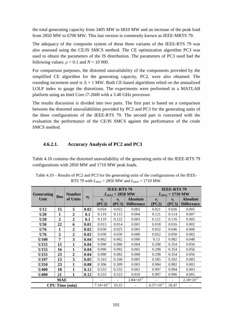
101

the total generating capacity from 3405 MW to 6810 MW and an increase of the peak load from 2850 MW to 6700 MW. This last version is commonly known as IEEE-MRTS 79.

The adequacy of the composite system of these three variants of the IEEE-RTS 79 was also assessed using the CE/IS SMCS method. The CE optimization algorithm PC3 was used to obtain the parameters of the IS distribution. The parameters of PC3 used had the following values: ρ = 0.1 and N = 10 000.

For comparison purposes, the distorted unavailability of the components provided by the simplified CE algorithm for the generating capacity, PC2, were also obtained. The rounding increment used is ∆ = 1 MW. Both CE-based algorithms relied on the annualized LOLP index to gauge the distortions. The experiments were performed in a MATLAB platform using an Intel Core i7-2600 with a 3.40 GHz processor.

The results discussion is divided into two parts. The first part is based on a comparison between the distorted unavailabilities provided by PC2 and PC3 for the generating units of the three configurations of the IEEE-RTS 79. The second part is concerned with the evaluation the performance of the CE/IS SMCS against the performance of the crude SMCS method.

4.6.2.1. Accuracy Analysis of PC2 and PC3

Table 4.10 contains the distorted unavailability of the generating units of the IEEE-RTS 79 configurations with 2850 MW and 1710 MW peak loads.

Table 4.10 – Results of PC2 and PC3 for the generating units of the configurations of the IEEE-RTS 79 with LMAX = 2850 MW and LMAX = 1710 MW.

Generating Unit

Bus Number of Units

uj

IEEE-RTS 79 LMAX = 2850 MW

IEEE-RTS 79 LMAX = 1710 MW

vj (PC2)

vj (PC3)

Absolute Difference

vj (PC2)

vj (PC3)

Absolute Difference

U12 15 5 0.02 0.024 0.022 0.002 0.021 0.026 0.005 U20 1 2 0.1 0.119 0.115 0.004 0.121 0.114 0.007 U20 2 2 0.1 0.119 0.122 0.003 0.121 0.116 0.005 U50 22 6 0.01 0.013 0.014 0.001 0.018 0.016 0.002 U76 1 2 0.02 0.030 0.025 0.005 0.052 0.046 0.006 U76 2 2 0.02 0.030 0.030 0.000 0.052 0.050 0.002 U100 7 3 0.04 0.062 0.062 0.000 0.13 0.082 0.048 U155 15 1 0.04 0.090 0.086 0.004 0.298 0.354 0.056 U155 16 1 0.04 0.090 0.092 0.002 0.298 0.354 0.056 U155 23 2 0.04 0.090 0.082 0.008 0.298 0.354 0.056 U197 13 3 0.05 0.163 0.168 0.005 0.585 0.502 0.083 U350 23 1 0.08 0.306 0.309 0.003 0.984 0.982 0.002 U400 18 1 0.12 0.533 0.532 0.001 0.997 0.994 0.003 U400 21 1 0.12 0.533 0.523 0.010 0.997 0.996 0.001

MAE - - 2.84×10-3 - - 2.18×10-2

CPU Time (min) 7.10×10-3 10.22 - 6.57×10-3 20.47 -

102

These distortions were obtained using PC2 and PC3. Note that PC2 was developed for the generating capacity adequacy assessment whereas PC3 is able to provide distortions for the generating units and the transmission circuits. This table also presents the MAE for the distorted parameters vj to help compare the distortions provided by PC2 and PC3. The references used for calculating the MAE are the distortions provided by PC3 since this is the pure CE optimization algorithm for the composite system. The CPU time of PC2 and PC3 is also reported in Table 4.10.

In theory, the parameters vj of the iid generating units connected at the same bus should be equal. However, since PC3 samples the state for all units individually, the distortions of these units can be different. To obtain equal distortion for these units, their respective parameters vj were averaged.

The results in Table 4.10 show that the difference between the distorted unavailability provided by the two CE algorithms for the composite system of the IEEE-RTS 79 with 2850 MW peak load is small. In other words, PC2 and PC3 were able provide equivalent vj for all generating units even for those whose unavailability has changed the most.

In contrast, some important differences between the distortions provided by PC2 and PC3 were observed for the case of the LMAX = 1710 MW. Despite the fact most of the parameters vj obtained by the two CE-based algorithms are similar, the two distortions for the units U197 at bus 13 have an absolute difference of 0.083. This result shows that the distorted unavailability of the generating units can be greatly affected by the transmission network even when loss of load is rare.

As a last remark, note that the CPU time of PC2 and PC3 reported in Table 4.10 is considerably different. As a matter of fact, PC2 evaluates generation states whereas PC3 assesses composite states. This makes PC3 computationally more demanding than PC2, which is mainly caused by the time-consuming optimization process represented by (4.54).

Table 4.11 contains the parameter vj for the transmission circuits of the same two configurations of the IEEE-RTS 79. These parameters were obtained with PC3. As a matter of fact, PC3 estimates not only the optimal CE distorted unavailability of the generating units but also of the transmission circuits. On the contrary, PC2 can only calculate the distorted unavailability of the generating units.

The results in Table 4.11 show that the distorted unavailability of the transmission circuits of the original configuration of the IEEE-RTS 79 (i.e., LMAX = 2850 MW) is almost equal to the original parameter uj.

Moreover, the distortions obtained for the 1710 MW peak load indicate that the parameter vj of the transmission circuits tends to zero as the system becomes reliable.

The accuracy of PC2 and PC3 was also tested for the IEEE-MRTS 79, which is a system known for its stressed transmission system [5]. Accordingly, the distorted unavailability of the generating units provided by the two CE algorithms was compared. The parameters vj of the generating units are reported in Table 4.12. Conversely,

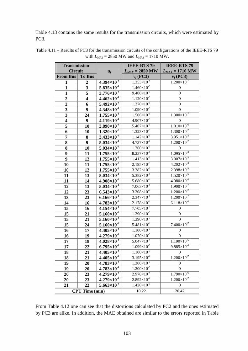
103

Table 4.13 contains the same results for the transmission circuits, which were estimated by PC3.

Table 4.11 – Results of PC3 for the transmission circuits of the configurations of the IEEE-RTS 79 with LMAX = 2850 MW and LMAX = 1710 MW.

Transmission Circuit uj

IEEE-RTS 79 LMAX = 2850 MW

IEEE-RTS 79 LMAX = 1710 MW

From Bus To Bus vj (PC3) vj (PC3) 1 2 4.394×10-4 1.353×10-4 1.200×10-7 1 3 5.835×10-4 1.460×10-6 0 1 5 3.776×10-4 9.400×10-7 0 2 4 4.462×10-4 1.120×10-6 0 2 6 5.492×10-4 1.370×10-6 0 3 9 4.348×10-4 1.090×10-6 0 3 24 1.755×10-3 1.506×10-3 1.300×10-7 4 9 4.119×10-4 4.907×10-3 0 5 10 3.890×10-4 5.407×10-5 1.010×10-6 6 10 1.320×10-3 1.323×10-3 1.300×10-7 7 8 3.433×10-4 1.142×10-3 3.951×10-3 8 9 5.034×10-4 4.737×10-4 1.200×10-7 8 10 5.034×10-4 1.260×10-6 0 9 11 1.755×10-3 8.237×10-4 1.095×10-3 9 12 1.755×10-3 1.413×10-3 3.007×10-3 10 11 1.755×10-3 2.195×10-3 4.202×10-3 10 12 1.755×10-3 3.382×10-3 2.398×10-3 11 13 5.034×10-4 5.382×10-4 1.520×10-6 11 14 4.908×10-4 5.680×10-4 4.980×10-4 12 13 5.034×10-4 7.063×10-4 1.900×10-7 12 23 6.543×10-4 3.208×10-4 1.200×10-7 13 23 6.166×10-4 2.347×10-4 1.200×10-7 14 16 4.783×10-4 2.178×10-4 6.118×10-4 15 16 4.154×10-4 7.705×10-3 0 15 21 5.160×10-4 1.290×10-6 0 15 21 5.160×10-4 1.290×10-6 0 15 24 5.160×10-4 5.481×10-4 7.400×10-7 16 17 4.405×10-4 1.100×10-6 0 16 19 4.279×10-4 1.070×10-6 0 17 18 4.028×10-4 5.047×10-4 1.190×10-6 17 22 6.795×10-4 1.099×10-3 9.885×10-4 18 21 4.405×10-4 1.100×10-6 0 18 21 4.405×10-4 3.195×10-4 1.200×10-7 19 20 4.783×10-4 1.200×10-6 0 19 20 4.783×10-4 1.200×10-6 0 20 23 4.279×10-4 2.978×10-4 1.790×10-6 20 23 4.279×10-4 2.892×10-4 1.200×10-7 21 22 5.663×10-4 1.420×10-6 0

CPU Time (min) 10.22 20.47

From Table 4.12 one can see that the distortions calculated by PC2 and the ones estimated by PC3 are alike. In addition, the MAE obtained are similar to the errors reported in Table

104

4.10 for the respective configurations of the IEEE-RTS 79 analyzed. On the other hand, the analysis of the absolute errors for each generating unit in Table 4.12 reveals that the worst absolute difference registered was 0.159, which is precisely for the case of the generating units that experienced the highest distortion.

This significant difference indicates that the use of PC2 instead of PC3 must be parsimonious in the case of stressed transmission systems.

Table 4.12 – Results of PC2 and PC3 for the generating units of the IEEE-MRTS 79.

Generating Unit Bus

Number of Units uj

vj (PC2)

vj (PC3)

Absolute Difference

U24 15 5 0.02 0.024 0.024 0.000 U40 1 2 0.1 0.119 0.125 0.006 U40 2 2 0.1 0.119 0.115 0.004 U100 22 6 0.01 0.013 0.013 0.000 U152 1 2 0.02 0.030 0.039 0.009 U152 2 2 0.02 0.030 0.035 0.005 U200 7 3 0.04 0.062 0.059 0.003 U310 15 1 0.04 0.090 0.090 0.000 U310 16 1 0.04 0.090 0.101 0.011 U310 23 2 0.04 0.090 0.095 0.005 U394 13 3 0.05 0.163 0.129 0.034 U700 23 1 0.08 0.306 0.333 0.027 U800 18 1 0.12 0.533 0.378 0.155 U800 21 1 0.12 0.533 0.374 0.159

MAE - - 1.63×10-2

CPU Time (min) 7.10×10-3 5.37 -

Consider now the results in Table 4.13. A careful review of the distortions in this table tells that the parameters vj obtained for the transmission circuits of the IEEE-MRTS 79 are not very different from the original parameters uj. However, the results in Table 4.10 and Table 4.12 indicate that the transmission system can significantly affect the parameter vj of the generating units.

This counterintuitive result is easily justified from the examination of (4.39). As a matter of fact, this equation shows that the components involved more often in the loss of load events, i.e., the components which are in the down state when load is curtailed, are the ones whose unavailability is distorted the most.

In the case of the IEEE-MRTS 79, PC3 can easily detect which generating units are down in failure events. The same is not true for the transmission circuits since most of the loss of load events involving the network of the IEEE-MRTS 79 is caused by shortage of transmission capacity rather than by forced outages of its circuits [5].

As a final remark, the loading status of the transmission network and its topology can have an important impact on the distortion of not only the unavailability of the generating units and but also on the unavailability of the transmission circuits. For that reason, the optimal CE parameters vj for composite systems can only be obtained accurately using PC3.

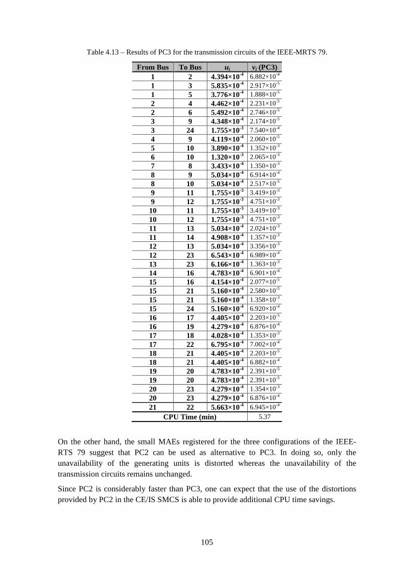
105

Table 4.13 – Results of PC3 for the transmission circuits of the IEEE-MRTS 79.

From Bus To Bus uj vj (PC3) 1 2 4.394×10-4 6.882×10-4 1 3 5.835×10-4 2.917×10-5 1 5 3.776×10-4 1.888×10-5 2 4 4.462×10-4 2.231×10-5 2 6 5.492×10-4 2.746×10-5 3 9 4.348×10-4 2.174×10-5 3 24 1.755×10-3 7.540×10-4 4 9 4.119×10-4 2.060×10-5 5 10 3.890×10-4 1.352×10-3 6 10 1.320×10-3 2.065×10-3 7 8 3.433×10-4 1.350×10-3 8 9 5.034×10-4 6.914×10-4 8 10 5.034×10-4 2.517×10-5 9 11 1.755×10-3 3.419×10-3 9 12 1.755×10-3 4.751×10-3 10 11 1.755×10-3 3.419×10-3 10 12 1.755×10-3 4.751×10-3 11 13 5.034×10-4 2.024×10-3 11 14 4.908×10-4 1.357×10-3 12 13 5.034×10-4 3.356×10-3 12 23 6.543×10-4 6.989×10-4 13 23 6.166×10-4 1.363×10-3 14 16 4.783×10-4 6.901×10-4 15 16 4.154×10-4 2.077×10-5 15 21 5.160×10-4 2.580×10-5 15 21 5.160×10-4 1.358×10-3 15 24 5.160×10-4 6.920×10-4 16 17 4.405×10-4 2.203×10-5 16 19 4.279×10-4 6.876×10-4 17 18 4.028×10-4 1.353×10-3 17 22 6.795×10-4 7.002×10-4 18 21 4.405×10-4 2.203×10-5 18 21 4.405×10-4 6.882×10-4 19 20 4.783×10-4 2.391×10-5 19 20 4.783×10-4 2.391×10-5 20 23 4.279×10-4 1.354×10-3 20 23 4.279×10-4 6.876×10-4

21 22 5.663×10-4 6.945×10-4

CPU Time (min) 5.37

On the other hand, the small MAEs registered for the three configurations of the IEEE-RTS 79 suggest that PC2 can be used as alternative to PC3. In doing so, only the unavailability of the generating units is distorted whereas the unavailability of the transmission circuits remains unchanged.

Since PC2 is considerably faster than PC3, one can expect that the use of the distortions provided by PC2 in the CE/IS SMCS is able to provide additional CPU time savings.

106

4.6.2.2. Performance Analysis of PC2 and PC3

The composite system of three configurations of the IEEE-RTS 79 analyzed in the previous section was assessed using the crude SMCS and the CE/IS SMCS methods. As a matter of fact, the CE/IS SMCS method used not only the distorted parameters calculated by PC2 but also the ones estimated PC3. Since PC2 can only provide the parameters vj for the generating units, it was assumed in the respective CE/IS-based sequential simulation that the parameter vj of the transmission circuits is equal to its original parameter uj. All simulations were stopped when the estimates of the annual reliability indexes had a β ≤ 5% or when 5000 years were simulated. In the case of the simulations ended by the last stopping criterion, the coefficient of variation of the estimates of the reliability indices was saved. This coefficient is presented in between brackets alongside the respective estimate. All the experiments were performed in a MATLAB platform using an Intel Core i7-2600 with a 3.40 GHz processor.

Table 4.14 contains the results for the composite system of the IEEE-RTS 79 with LMAX = 2850 MW. This table is divided into two parts. The first part of Table 4.14 holds the states evaluated by PC2 and PC3 and the respective CPU time. The number of states evaluated by PC2 cannot be obtained since this CE-based algorithm is based on convolution operations. On the contrary, all evaluations can be accounted for in the case of PC3 since this algorithm relies on the non-sequential MCS method.

Table 4.14 – Results of PC2 and PC3 for the composite system of the IEEE-RTS 79 with LMAX = 2850 MW.

IEEE-RTS 79 LMAX = 2850 MW

PC2 Generation States Evaluated -

CPU Time (min) 7.10×10-3

PC3 Composite States Evaluated 20 000

CPU Time (min) 10.22

Crude SMCS

CE/IS SMCS (PC2)

CE/IS SMCS (PC3)

SMCS

Composite States Evaluated 19 757 457 386 025 289 697 Years Simulated 2142 40 30 CPU Time (min) 9879.03 193.04 144.50

LOLE (h/yr) 10.700 10.566 10.382 EENS (MWh/yr) 1312.26 1302.29 1319.95 LOLF (occ./yr) 2.246 2.176 2.207

The second part of Table 4.14 contains the estimates of the annual reliability indices for the composite system of the IEEE-RTS 79 with 2850 MW peak load. The evaluations carried out by the CE/IS SMCS method used two different sampling distributions f(X; v), according to the results provided by PC2 and PC3. The parameters vj of these two different IS distributions are presented in Table 4.10 and Table 4.11.The CPU time reported in the second part of Table 4.14 refers only to the sequential simulation and does not include the

107

CPU time of PC2 and PC3. The number of composite states evaluated by the crude and the CE/IS SMCS methods is also indicated.

First of all, the results in Table 4.14 shows that the estimates of the reliability indices of the composite system provided by the crude and the CE/IS SMCS methods for the configurations of the IEEE-RTS 79 evaluated are equivalent, which is in line with the fact that the IS technique does not affect the accuracy of the estimates of the reliability indices.

Moreover, the crude SMCS method has required 2142 years of simulation whereas the CE/IS SMCS (PC2) method has simulated 40 years and the CE/IS SMCS (PC3) only 30. To calculate the net speed up, the CPU time required by PC2 and PC3 as well as the time of the respective IS sequential simulations must be taken into account. Accordingly, the execution of PC2 and the CE/IS SMCS (PC2) was 51.18 times faster than the crude SMCS. In opposition, the equivalent gain provided by PC3 and the CE/IS SMCS (PC3) is 63.85. Hence, the CPU time required by PC3 and the respective CE/IS-based sequential simulation is less than the time taken by PC2 and the CE/IS SMCS (PC2).

These different gains in efficiency can be explained by the less 76 328 composite state evaluations made by PC3 and the CE/IS SMCS (PC3) as compared to the CE/IS SMCS (PC2) method. In addition, the ratios between the composite states evaluated by the crude SMCS method and by the CE/IS-based sequential simulations are very similar to the net speed ups. Actually, the ratio between the states evaluated by the crude and the CE/IS SMCS (PC2) methods is precisely 51.18. This same ratio is 63.80 when the total number of composite states evaluated by PC3 and the CE/IS SMCS (PC3) is compared with the total number of evaluations made by the crude SMCS method. This is consistent with the fact that most of the time spent in the adequacy assessment of composite systems is in the state evaluation stage.

Table 4.15 presents the results for the composite system of the IEEE-RTS 79 with a 1710 MW peak load. Like in the case of the 2850 MW peak load, Table 4.15 is divided into two parts.

Table 4.15 – Results of PC2 and PC3 for the composite system of the IEEE-RTS 79 with LMAX =1710 MW.

IEEE-RTS 79 LMAX = 1710 MW

PC2 Generation States Evaluated -

CPU Time (min) 6.57×10-3

PC3 Composite States Evaluated 40 000

CPU Time (min) 20.47

Crude SMCS

CE/IS SMCS (PC2)

CE/IS SMCS (PC3)

SMCS

Composite States Evaluated 46 119 847 714 832 537 577

Years Simulated 5000 66 50

CPU Time (min) 23 060.10 357.13 268.52

LOLE (h/yr) 1.324×10-3 (71.58%) 1.113×10-4 1.097×10-4

EENS (MWh/yr) 7.04×10-2 (77.72%) 5.74×10-3 5.73×10-3

LOLF (occ./yr) 4.000×10-3 (70.77%) 3.731×10-5 3.743×10-5

108

The first part refers to the number of states and the CPU time of PC2 and PC3 while the second part is related to the results provided by the crude and the CE/IS SMCS methods. The second part of this table contains not only the estimates of the reliability indices obtained by the crude SMCS method and by the two CE/IS-based sequential simulations but also the number of composite states evaluated and the respective CPU times.

First of all, the results Table 4.15 show that the CPU time of PC2 is, once again, incomparably smaller than the time taken by PC3. Note that the CPU time of PC3 is almost twice the time spent by this same algorithm for the configuration of the IEEE-RTS 79 with a 2850 MW peak load (see Table 4.14). This result agrees with the fact that PC3 needs the double of the composite state evaluations in this case than in case of the configuration of the IEEE-RTS 79 with LMAX = 2850 MW.

Table 4.15 also indicates that the crude SMCS method was not able to obtain estimates for the reliability indices in 5000 simulated years with a β ≤ 5%. In opposition, the CE/IS SMCS (PC2) and the CE/IS SMCS (PC3) provided accurate estimates with only 66 and 50 years of simulation, respectively.

For this reason, the net speed up cannot be accurately computed since the estimates provided by the crude and the CE/IS SMCS methods have dissimilar accuracies. All the same, a pessimistic net speed up can still be calculated with the results in Table 4.15. Accordingly, the CE/IS SMCS method that used the sampling distribution calculated by PC2 has taken 357.13 minutes. Conversely, the net CPU time is 288.99 minutes when the sampling distribution estimated by PC3 is used by the CE/IS SMCS method.

These CPU times correspond to a net speed up of 64.57 in the case of the CE/IS SMCS (PC2) whereas the gain is 79.89 in the case of the CE/IS SMCS (PC3). Once again, the less number of composite states evaluated by PC3 and CE/IS SMCS (PC3) is the cause for this difference in efficiency.

Hence, PC3 can require more CPU time than PC2 to estimate the distorted unavailability for the components of the system. However, the time lost is easily recovered in the subsequent sequential simulation due to fewer composite state evaluations.

Table 4.16 – Results of PC2 and PC3 for the composite system of the IEEE-MRTS 79.

IEEE-MRTS 79

PC2 Generation States Evaluated -

CPU Time (min) 7.10×10-3

PC3 Composite States Evaluated 10 000

CPU Time (min) 5.37

Crude SMCS

CE/IS SMCS (PC2)

CE/IS SMCS (PC3)

SMCS

Composite States Evaluated 9 030 171 3 330 697 2 682 853

Years Simulated 979 345 279

CPU Time (min) 4514.68 1665.15 1341.52

LOLE (h/yr) 37.764 36.658 36.466

EENS (MWh/yr) 6037.72 5833.21 5758.73

LOLF (occ./yr) 7.596 7.522 7.661

109

The results for the IEEE-MRTS 79 are presented in Table 4.16. Once again, this table is divided into two parts. The first part contains the number of states and CPU time of PC2 and PC3. In turn, the second part of Table 4.16 presents the estimates of the composite system reliability indices provided by the crude and the CE/IS SMCS methods. This second part also contains the number of composite states evaluated and the respective CPU time spent.

The results in Table 4.16 show that only 10 000 composite state evaluations were required by PC3 to estimate the distorted unavailability of the generating units and transmission circuits of the IEEE-MRTS 79. In this case, PC3 has converged in the first iteration. The equivalent analysis for the two configurations of the IEEE-RTS 79 previously analyzed, reveals that two iterations of PC3 were needed in the case of the 2850 MW peak load whereas 4 iterations were required for the configuration with LMAX = 1710 MW. Therefore, the number of composite states evaluated by PC3 decreases as the system becomes less reliable. Moreover, the results of the composite system adequacy assessment presented in the second part of Table 4.16 demonstrate that the CE/IS SMCS (PC2) and the CE/IS SMCS (PC3) methods obtained net speed ups of 2.71 and 3.35, respectively, over the crude SMCS method. Compared with the greater speed ups obtained for the previously analyzed configurations of the IEEE-RTS 79, these results are somehow disappointing. Hence, the IS distributions provided by PC2 and PC3 cannot provide a variance reduction for the IEEE-MRTS 79 as effective as the one obtained for the previously analyzed configurations of the IEEE-RTS 79.

Actually, the speed up that can be achieved by using the PC3 and the CE/IS SMCS (PC3) method is 63.85 for the case of the original peak load of the IEEE-RTS 79, increases to a pessimistic estimate of 79.89 when the peak load of the IEEE-RTS 79 is reduced by a factor of 0.6 (i.e., when the system becomes very reliable), and decreases considerably to 3.35 when the transmission system of the IEEE-RTS 79 is stressed (i.e., when the system becomes unreliable).

These different results show that the time-efficiency of the CE/IS-based sequential simulations over the crude SMCS method is strongly affected by how reliable the system is: the more reliable the system, the greater the speed up. In some cases, like the IEEE-MRTS 79, the use of the CE/IS-based sequential simulation might not pay off since the small time gains may not offset the inaccurate probability distributions of the reliability indices provided by this method. Even so, the use of CE method and IS is indeed one of the best approaches to reduce considerably the number of state evaluations required to obtain accurate estimates of the reliability indices, i.e., to improve the efficiency of the sequential MCS method.

It is also worth remarking that that the CE/IS SMCS (PC3) method was consistently the most time-efficient approach in all simulations carried out. However, the loss in net CPU time of the CE/IS SMCS (PC2) method was not considerable. Hence, the use the distortions provided by PC2 can be a feasible and much simpler alternative to the full CE optimization algorithm for the composite system (PC3).

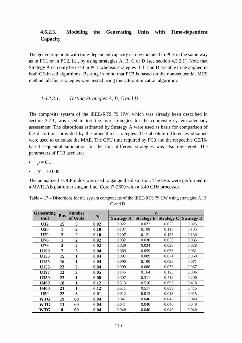
110

4.6.2.3. Modeling the Generating Units with Time-dependent Capacity

The generating units with time-dependent capacity can be included in PC3 in the same way as in PC1 or in PC2, i.e., by using strategies A, B, C or D (see section 4.5.2.1). Note that Strategy A can only be used in PC1 whereas strategies B, C and D are able to be applied in both CE-based algorithms. Bearing in mind that PC3 is based on the non-sequential MCS method, all four strategies were tested using this CE optimization algorithm.

4.6.2.3.1. Testing Strategies A, B, C and D

The composite system of the IEEE-RTS 79 HW, which was already been described in section 3.7.1, was used to test the four strategies for the composite system adequacy assessment. The distortions estimated by Strategy A were used as basis for comparison of the distortions provided by the other three strategies. The absolute differences obtained were used to calculate the MAE. The CPU time required by PC3 and the respective CE/IS-based sequential simulation for the four different strategies was also registered. The parameters of PC3 used are:

• ρ = 0.1

• N = 10 000.

The annualized LOLP index was used to gauge the distortion. The tests were performed in a MATLAB platform using an Intel Core i7-2600 with a 3.40 GHz processor.

Table 4.17 – Distortions for the system components of the IEEE-RTS 79 HW using strategies A, B, C and D.

Generating Unit

Bus Number of Units

uj vj

Strategy A Strategy B Strategy C Strategy D U12 15 5 0.02 0.022 0.022 0.025 0.025 U20 1 2 0.10 0.107 0.109 0.116 0.135 U20 2 2 0.10 0.107 0.121 0.126 0.130 U76 1 2 0.02 0.032 0.030 0.030 0.035 U76 2 2 0.02 0.029 0.034 0.026 0.028 U100 7 3 0.04 0.069 0.059 0.056 0.061 U155 15 1 0.04 0.091 0.089 0.074 0.060 U155 16 1 0.04 0.090 0.100 0.093 0.071 U155 23 2 0.04 0.099 0.086 0.076 0.067 U197 13 3 0.05 0.145 0.164 0.125 0.086 U350 23 1 0.08 0.307 0.311 0.412 0.206 U400 18 1 0.12 0.513 0.516 0.692 0.418 U400 21 1 0.12 0.511 0.517 0.689 0.415 U50 22 6 0.01 0.012 0.012 0.013 0.015

WTG 19 80 0.04 0.041 0.040 0.040 0.040 WTG 11 60 0.04 0.041 0.040 0.040 0.040 WTG 8 60 0.04 0.040 0.040 0.040 0.040

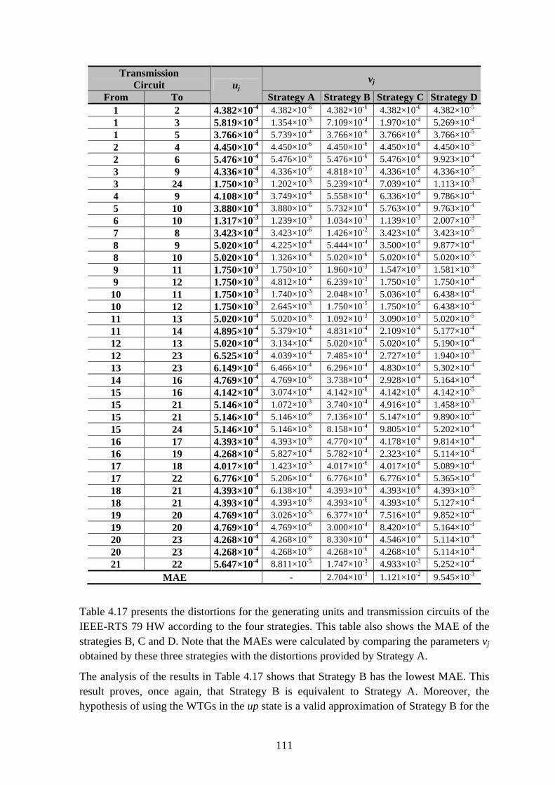
111

Transmission Circuit uj

vj

From To Strategy A Strategy B Strategy C Strategy D 1 2 4.382×10-4 4.382×10-6 4.382×10-6 4.382×10-6 4.382×10-5 1 3 5.819×10-4 1.354×10-3 7.109×10-4 1.970×10-4 5.269×10-4 1 5 3.766×10-4 5.739×10-4 3.766×10-6 3.766×10-6 3.766×10-5 2 4 4.450×10-4 4.450×10-6 4.450×10-6 4.450×10-6 4.450×10-5 2 6 5.476×10-4 5.476×10-6 5.476×10-6 5.476×10-6 9.923×10-4 3 9 4.336×10-4 4.336×10-6 4.818×10-3 4.336×10-6 4.336×10-5 3 24 1.750×10-3 1.202×10-3 5.239×10-4 7.039×10-4 1.113×10-3 4 9 4.108×10-4 3.749×10-4 5.558×10-4 6.336×10-4 9.786×10-4 5 10 3.880×10-4 3.880×10-6 5.732×10-4 5.763×10-4 9.763×10-4 6 10 1.317×10-3 1.239×10-3 1.034×10-3 1.139×10-3 2.007×10-3 7 8 3.423×10-4 3.423×10-6 1.426×10-2 3.423×10-6 3.423×10-5 8 9 5.020×10-4 4.225×10-4 5.444×10-4 3.500×10-4 9.877×10-4 8 10 5.020×10-4 1.326×10-4 5.020×10-6 5.020×10-6 5.020×10-5 9 11 1.750×10-3 1.750×10-5 1.960×10-3 1.547×10-3 1.581×10-3 9 12 1.750×10-3 4.812×10-4 6.239×10-3 1.750×10-5 1.750×10-4 10 11 1.750×10-3 1.740×10-3 2.048×10-3 5.036×10-4 6.438×10-4 10 12 1.750×10-3 2.645×10-3 1.750×10-5 1.750×10-5 6.438×10-4 11 13 5.020×10-4 5.020×10-6 1.092×10-3 3.090×10-3 5.020×10-5 11 14 4.895×10-4 5.379×10-4 4.831×10-4 2.109×10-4 5.177×10-4 12 13 5.020×10-4 3.134×10-4 5.020×10-6 5.020×10-6 5.190×10-4 12 23 6.525×10-4 4.039×10-4 7.485×10-4 2.727×10-4 1.940×10-3 13 23 6.149×10-4 6.466×10-4 6.296×10-4 4.830×10-4 5.302×10-4 14 16 4.769×10-4 4.769×10-6 3.738×10-4 2.928×10-4 5.164×10-4 15 16 4.142×10-4 3.074×10-4 4.142×10-6 4.142×10-6 4.142×10-5 15 21 5.146×10-4 1.072×10-3 3.740×10-4 4.916×10-4 1.458×10-3 15 21 5.146×10-4 5.146×10-6 7.136×10-4 5.147×10-4 9.890×10-4 15 24 5.146×10-4 5.146×10-6 8.158×10-4 9.805×10-4 5.202×10-4 16 17 4.393×10-4 4.393×10-6 4.770×10-4 4.178×10-4 9.814×10-4 16 19 4.268×10-4 5.827×10-4 5.782×10-4 2.323×10-4 5.114×10-4 17 18 4.017×10-4 1.423×10-3 4.017×10-6 4.017×10-6 5.089×10-4 17 22 6.776×10-4 5.206×10-4 6.776×10-6 6.776×10-6 5.365×10-4 18 21 4.393×10-4 6.138×10-4 4.393×10-6 4.393×10-6 4.393×10-5 18 21 4.393×10-4 4.393×10-6 4.393×10-6 4.393×10-6 5.127×10-4 19 20 4.769×10-4 3.026×10-5 6.377×10-4 7.516×10-4 9.852×10-4 19 20 4.769×10-4 4.769×10-6 3.000×10-4 8.420×10-4 5.164×10-4 20 23 4.268×10-4 4.268×10-6 8.330×10-4 4.546×10-4 5.114×10-4 20 23 4.268×10-4 4.268×10-6 4.268×10-6 4.268×10-6 5.114×10-4 21 22 5.647×10-4 8.811×10-5 1.747×10-3 4.933×10-3 5.252×10-4

MAE - 2.704×10-3 1.121×10-2 9.545×10-3

Table 4.17 presents the distortions for the generating units and transmission circuits of the IEEE-RTS 79 HW according to the four strategies. This table also shows the MAE of the strategies B, C and D. Note that the MAEs were calculated by comparing the parameters vj obtained by these three strategies with the distortions provided by Strategy A.

The analysis of the results in Table 4.17 shows that Strategy B has the lowest MAE. This result proves, once again, that Strategy B is equivalent to Strategy A. Moreover, the hypothesis of using the WTGs in the up state is a valid approximation of Strategy B for the

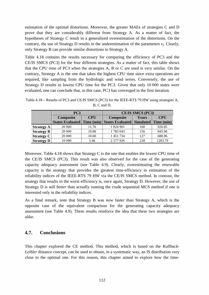
112

estimation of the optimal distortions. Moreover, the greater MAEs of strategies C and D prove that they are considerably different from Strategy A. As a matter of fact, the hypotheses of Strategy C result in a generalized overestimation of the distortions. On the contrary, the use of Strategy D results in the underestimation of the parameters vj. Clearly, only Strategy B can provide similar distortions to Strategy A.

Table 4.18 contains the results necessary for comparing the efficiency of PC3 and the CE/IS SMCS (PC3) for the four different strategies. As a matter of fact, this table shows that the CPU time of PC3 when the strategies A, B or C are used is very similar. On the contrary, Strategy A is the one that takes the highest CPU time since extra operations are required, like sampling from the hydrologic and wind series. Conversely, the use of Strategy D results in lowest CPU time for the PC3. Given that only 10 000 states were evaluated, one can conclude that, in this case, PC3 has converged in the first iteration.

Table 4.18 – Results of PC3 and CE/IS SMCS (PC3) for the IEEE-RTS 79 HW using strategies A, B, C and D.

PC3 CE/IS SMCS (PC3) Composite

States Evaluated CPU

Time (min) Composite

States Evaluated Years

Simulated CPU

Time (min) Strategy A 20 000 11.76 1 824 901 160 926.85 Strategy B 20 000 10.88 1 785 643 156 845.96 Strategy C 20 000 10.60 1 451 734 127 688.96 Strategy D 10 000 5.46 2 577 926 228 1283.79

Moreover, Table 4.18 shows that Strategy C is the one that enables the lowest CPU time of the CE/IS SMCS (PC3). This result was also observed for the case of the generating capacity adequacy assessment (see Table 4.9). Clearly, overestimating the renewable capacity is the strategy that provides the greatest time-efficiency in estimation of the reliability indices of the IEEE-RTS 79 HW via the CE/IS SMCS method. In contrast, the strategy that results in the worst efficiency is, once again, Strategy D. However, the use of Strategy D is still better than actually running the crude sequential MCS method if one is interested only in the reliability indices.

As a final remark, note that Strategy B was now faster than Strategy A, which is the opposite case of the equivalent comparison for the generating capacity adequacy assessment (see Table 4.9). These results reinforce the idea that these two strategies are alike.

4.7. Conclusions

This chapter explored the CE method. This method, which is based on the Kullback-Leibler distance concept, can be used to obtain, in a systematic way, an IS distribution very close to the optimal one. For this reason, this chapter aimed to explore how the time-

113

efficiency of the sequential MCS method can be improved by using the IS technique with parameters optimized by the CE method.

The chapter started with an overview of the VRTs that have been applied to the adequacy assessment of power systems. Subsequently, the theory supporting the IS technique and the CE method was duly presented. Next, the analysis of the equations of the standard CE optimization algorithm for the generating capacity adequacy assessment (PC1) has demonstrated that the CE-optimal IS distribution can be obtained by simply dividing the annualized reliability indices of different configurations of the system. As a result, a new CE-based algorithm (PC2) for the generating capacity was proposed. This new CE-based algorithm can replace PC1 by a simple analytical procedure based on discrete convolution operations.

The new PC2 has been tested against the standard PC1 using several generating systems, including the IEEE-RTS 79, the IEEE-RTS 96, and two configurations of the SSB planned for the 90’s. In all cases, the results indicate that PC2 is equivalent to PC1 in both accuracy and computational performance. However, PC2 is much easier to be implemented, making it an excellent alternative to the standard CE optimization algorithm. In addition, the accuracy and computational performance of PC2 in real applications can be easily controlled with the capacity rounding increment ∆.

The savings in CPU time achievable by the using the CE method and the IS technique instead of the crude sequential MCS method were investigated for the generating capacity adequacy assessment. The results obtained showed that the savings in CPU time are greater as the system becomes more reliable. This speed up is possible due to an increased sampling efficiency of the CE/IS-based sequential simulation as opposed to that of the crude sequential MCS method. The drawback of using the IS technique with the sequential MCS method is that the information necessary to obtain the probability distributions of the reliability indices is lost. However, the flexibility of the sequential MCS method to represent time-varying loads, renewable power capacity fluctuation, scheduled maintenance schemes, etc. is retained.

This chapter also investigated how the generating units with time-dependent capacity can be included in PC1 and PC2. For this purpose, four strategies were proposed:

• Strategy A – random sampling of realizations of the generating capacities from the annual series;

• Strategy B – calculating the average capacity of the unit from the annual series and use it as the capacity that the unit provides in the up state;

• Strategy C – selecting the maximum capacity of the unit from the annual series and use it as the capacity that the unit provides in the up state;

• Strategy D – selecting the minimum capacity of the unit from the annual series and use it as the capacity that the unit provides in the up state.

114

Strategies B, C and D also assume that the wind turbines are always available. Moreover, Strategy A can only be used in the case of PC1 whereas strategies B, C and D can be implemented by PC1 and PC2.

After the analysis of the results obtained for the generating capacity and the composite system of the IEEE-RTS 79 HW, it was observed that Strategy C is the one that provides the highest simulation efficiency. Strategies A and B provided similar distortions and speed ups, which indicate that they are equivalent. In opposition, the use of Strategy D has led to the lowest gains in time. It is worth remarking that a different strategy may come up as the best one for a different power system since any of the four strategies proposed is able to accurately capture the time-dependency of the capacity of the generating units. Nevertheless, if one is interested in estimating solely the reliability indices, all these strategies can accelerate the adequacy assessment of systems with time-dependent units.

This chapter also proposed a CE optimization algorithm for the adequacy assessment of the composite system. This algorithm was named PC3. The distorted parameters of the generating units provided by PC3 were compared with the ones provided by PC2 (note that PC2 can only calculate the distortions for the generating units). This comparison demonstrated that, for the three variants of the IEEE-RTS 79 evaluated, the distortions calculated by PC2 are not very different from the ones estimated by PC3. In addition, the distorted parameters vj for the transmission circuits estimated by PC3 did not present significant dissimilarities from the original ones.

Bearing this in mind and knowing that PC2 is considerably faster than PC3, an investigation of the actual CPU time required to run the two CE-based algorithms and the respective CE/IS-based sequential simulations was promoted. Given that PC2 can only calculate distortions for the generating units, the respective CE/IS-based sequential simulation assumed that the unavailability of the transmissions circuits is unchanged. The results of these experiments showed that the time lost by PC3 is recovered in the subsequent CE/IS-based sequential simulation. This is due to the less composite state evaluations made by the CE/IS SMCS method when the distortions provided by PC3 are used instead of the ones calculated by PC2. Therefore, PC3 is the best choice for improving the efficiency of the sequential MCS method in the adequacy assessment of the composite system.

As a final remark, the speed ups obtained in the adequacy assessment of the composite system of configurations of the IEEE-RTS 79 corroborated the observations made for the case of the adequacy assessment of the generating capacity. Hence, as the composite power becomes more reliable, the gains in CPU time when using the IS technique with parameters optimized by the CE method become increasingly higher. Note that, when the composite system is very unreliable, like the case of the IEEE-MRTS 79, the speed up can be as little as 3.35, which is incomparably smaller than the gains obtained for the composite system of the IEEE-RTS 79 with 2850 MW and 1710 MW peak loads (note that the best speed ups for these configurations were, respectively, 63.80 and 79.89).

115

Chapter 5

Sequential Monte Carlo Simulation using Population-based Methods

5.1. Introduction

The previous chapter has proved that sampling efficiency of the sequential MCS method can be reduced by using the IS technique with parameters optimized by the CE method. The speed up of the sequential MCS method is achieved since the IS sampling distribution is optimized in a way that the variance of the estimators of the reliability indices is reduced. Consequently, the sampling process of the sequential MCS method if focused on the states that contribute to the estimates of the indices the most resulting in an effective decrease of the number of synthetically simulated years required to obtain accurate estimates of the indices.

The literature includes other possibilities to improve the time-efficiency of MCS methods. As a matter of fact, most of the time spent in the estimation of the reliability indices is when system states are being composed and evaluated [5], [6], [9], [22], [23], [29], [74], [75]. As a consequence, the state composition and evaluation steps, which often involve optimization procedures, can delay the sequential MCS method especially when the number of system states that need composition and evaluation is large [6]. Given the considerable number of system states composed and evaluated by the sequential MCS method, a small time gain on these steps will result in considerable savings in the total simulation time.

Several authors have proposed the substitution of the conventional mathematical tools used in the evaluation step by others that can perform similar task without significant loss of accuracy. Some of the earliest tools proposed belong to the field of contingency and topological analysis [145–149]. This research field is fruitful on tools that can detect circuit flow violation and apply remedial actions (e.g. generation rescheduling or load curtailment) to alleviate the overloaded circuits with minimum computational expense. Normally, these methods rely on mathematical models based on the linearization of the power flow equations. Note that these tools do not calculate exactly the optimal rescheduling for the generation units to eliminate the overloads of the circuits. As a consequence, additional load might be disconnected unnecessarily, which can result in inaccurate estimates of the reliability indices.

116

The CPU time of the state evaluation step can also be reduced through a different approach. As a matter of fact, the power system being assessed can be divided into different zones so that only a few are fully evaluated. Accordingly, the authors of [6] have proposed a division of power systems into three areas. The first area is named Equipment Outage Area and involves a complete representation of the random behavior of its components. The second area, which is named Optimization Area, includes the components that proceed to composition and evaluation. The generators and transmission circuits that are part of this second area but do not belong to the Equipment Outage Area are not allowed to fail. Nonetheless, the generators of the Optimization Area can be redispatched and the load curtailed. Finally, the third area, which is named External Area, connects the Optimization Area to the remaining components of the system. The generation and load of the External Area are fixed and modeled through equivalent models, like the Ward Equivalent [150]. The drawback of this approach is that it relies on localized optimizations which might lead to a suboptimal analysis. Once again, the reliability indices can be affected by considerable errors.

A different path that has been taken by many authors consists of dividing the steps of the MCS methods into several independent tasks that can be allocated to several processors and executed concurrently [13], [14]. This approach is based on the principle that large problems can be divided into smaller ones and be solved in parallel. Accordingly, three parallel topologies for scheduling the tasks of the non-sequential MCS are proposed in [13]. Conversely, two parallel methodologies for the adequacy assessment of the composite system via the sequential MCS are described in [14]. The first methodology proposed in [14] consists of the evaluation of the synthetically created years in parallel. Conversely, the second methodology is based on the evaluation of the system states within each simulated year in parallel and the convergence is checked by a dedicated processor at the end of the year.

A great attention has been paid recently to the OOP paradigm for the development software for the adequacy assessment of power systems [17]. Actually, OOP is a promising option to face the new challenges of producing computational tools for the electrical sector since it can provide the flexibility necessary to represent the complex behavior of the components of power systems and time-dependent issues [16], [18], [21]. Bearing this in mind, a flexible OOP programming algorithm for the adequacy assessment of the composite system via the non-sequential and the sequential MCS was proposed in [16].

The OOP paradigm also offers the possibility of using the ABT [18], [19], [21] for the development of flexible and intelligent simulation platforms. Taking advantage of this fact, an intelligent distributed environment that can incorporate and decide which methods should be used for the adequacy assessment of the generating capacity was developed in [21]. The intelligent agents of this distributed environment can choose between the non-sequential MCS, the sequential MCS method, and PBMs to compute accurate estimates of the reliability indices as fast as possible. For this purpose, different intelligent agents with different goals were defined, like the Sequence Producer Agent, the State Evaluator Agent and the Index Calculator Agent, and tasks of the process of estimating reliability indices were allocated to them. Intelligent agent communication architectures, namely the non-

117

synchronized and the synchronized approach, were also discussed and their benefits and drawbacks analyzed [20].

Recently, several authors have applied pattern recognition techniques [31] or classifiers, like ANN [27], SOM [28], GMDH [29], and LSVV [30] to perform classification of system states sampled before composition and evaluation. These classifiers are used to automatically detect the states that are more likely to have loss of load from those that do not. After this classification process, only the states that can have loss of load proceed to the state composition and evaluation.

These methods take advantage of the fact that the majority of the states composed and evaluated are success states, i.e., states that do not have loss of load. Hence considerable speed ups can be obtained by substituting the time-consuming composition and evaluation steps by an automatic pre-classification procedure. Obviously, this is only true if the automatic detection is faster than the composition and evaluation steps and if the collection of the data and the train of these classifiers are done in a fast way. The data used to train these classifiers is collected during the MCS methods. When sufficient data has been collected, the train of the classifiers is carried out. Hence, part of the simulation relies exclusively on the traditional composition and evaluation steps and the other part uses the classifier to detect which states should be evaluated or not.

The methodology proposed in this chapter stems from the concepts discussed in the last paragraph. In short, to avoid the composition and evaluation steps of the sequential MCS method, a two-stage methodology is proposed. Firstly, a list of states whose total capacity is inferior to the peak load is created using a PBM (the PBM used in this dissertation is based on the Evolutionary Particle Swarm Optimization (EPSO) [151] metaheuristic). Secondly, the states sampled by the sequential MCS method are compared to those on the list before proceeding to composition and evaluation. This comparison aims to emulate the pre-classification procedure carried out by the pattern recognition techniques previously discussed.

If state composition and evaluation should be performed, the yearly load model and the time-dependency of the capacity of the generators are chronologically followed to form system states. Note that these states may or may not have loss of load. If not, then it is automatically assumed that no loss of load occurs throughout the duration of these system states. To the knowledge of the author, the use of a PBM to obtain such list constitutes a new application of these methods.

It is worth mentioning that the use of lists to detect whether states should be composed and evaluated is not entirely new. As a matter of fact, an acceleration table created before the MCS method was proposed in [152]. This table, which was constructed based on screening all single and double outages of the transmission circuits, is used during the actual MCS method to decide which states should be composed and evaluated. The following sections briefly present PBMs, starting with an overview of their core: population-based metaheuristics.

118

5.2. Metaheuristic Optimization

Metaheuristics [35–37] are general-purpose iterative optimization methods that can tackle most of the optimization problems. Unlike pure mathematical methods, like the Simplex or the Newton-Raphson methods, metaheuristics do not guarantee that the optimal solution of the problem is found. Their main advantage is that they are capable of finding satisfactory solutions for complex and combinatorial optimization problems in reasonable time, which are precisely the ones that pure mathematical methods cannot or have great difficulties to solve.

In simple terms, metaheuristics are a way to find solutions, by trial and error, close to the optimum. These algorithms are often inspired by natural phenomena [36], [37], like ant colonies, the movements of flocks of birds or schools of fish, the Darwinian evolution and natural selection concepts, immune systems, and physical processes, like the annealing of metals. Generally, there are no mathematical proofs available to explain the convergence process of metaheuristics towards the optimum.

According to the No Free Lunch Theorem [153], the average quality of the solutions provided by any metaheuristic for all optimization problems is statistical identical, i.e., any high performance over one class of problems is counterbalanced by a poor performance over another class. Consequently, it is impossible to know in advance if the metaheuristic selected is going to provide good solutions for the optimization problem at hand or even which metaheuristic should be used to solve a given class of problems.

5.3. Convergence of Metaheuristics

The convergence of metaheuristics relies on two opposing forces: exploration and exploitation [154]. The exploration force aims to make the coverage of the space as broad as possible to avoid premature converge.

Figure 5.1 – Exploration vs. exploitation forces.

Generation

Fit

nes

s

Exploration

Exploitation

119

In contrast, the exploitation force narrows the search whenever a promising area of the space is found, hoping that even better solutions are discovered. An adequate balance between the exploration and exploitation forces is what makes a metaheuristic successful. Figure 5.1 depicts, for a minimization problem, the phase of the search where the exploration and exploitation forces are more intense.

To maintain an adequate diversity of solutions and, at the same time, to push the metaheuristic towards the optimum, two general operators are used [36], [37]: diversification and intensification.

Diversification is accomplished by cleverly randomizing current solutions. The role of this operator is to prevent the metaheuristic to become trapped at local optima. Each metaheuristic has its own mechanisms to create diversification. These mechanisms are a defining characteristic of the metaheuristic and are usually applied when new solutions are created.

In turn, the intensification operator is responsible for forcing the search towards the global optimum. This operator applies some sort of elitism to the search, i.e., it pushes the metaheuristic towards the zones of the space where the best performing solutions are. The intensification operator is usually employed to decide whether new solutions are kept or set aside. This decision takes the performance or fitness of the solutions into account. If a selection criterion based on pure elitism is used, the metaheuristic will systematically select the best solutions until it cannot discover better ones. Other selection criteria [36], like stochastic tournament, roulette wheel, etc., can be used to preserve the diversity of the search without compromising the selective pressure towards the optimum.

As depicted in Figure 5.1, the diversification operator plays a more important role at the beginning of the search. As the search advances towards the end, the importance of the diversification operator over selection gradually changes. The rate at which this change is made can be controlled by using strategic parameters [36]. These parameters are normally set at the beginning of the search. Self-adaptive schemes that try to mitigate the role of these parameters on the convergence process have also been proposed [36]. The self-adaptive schemes hope to make metaheuristics more robust against the values selected for the strategic parameters.

5.3.1. Trajectory-based vs. Population-based Metaheuristics

Metaheuristics can be divided as trajectory-based and population-based [37]. Trajectory-based metaheuristics improve iteratively a single solution. This type of metaheuristics can be viewed as walks through neighborhoods or as trajectories through the search space.

The unique solution represents the best solution found so far by the metaheuristics for the optimization problem being solved. Examples of trajectory-based metaheuristics are Local Search [155], Simulated Annealing [156], Greedy Randomized Adaptive Search Procedure [157] and Tabu Search [158].

120

In contrast, population-based metaheuristics start from an initial population of solutions. Normally, the size of the population is kept fixed, i.e., it is not allowed to increase or decrease during the search. Then, the diversification operator is applied to each solution of the current population to generate a slightly different population. After that, selection is carried out from the two populations to create a new one that will replace the current population.

Population-based metaheuristics repeat recursively this evolutionary process until a stopping criterion is satisfied. In the end, the population is filled with solutions that generally have a better performance than the ones in the initial population. The solution for the optimization problem being solved is the best performing individual of the last generation. Commonly used population-based metaheuristics are, among others, Genetic Algorithms (GA) [36], Evolution Strategies (ES) [36], Evolutionary Programming (EP) [36], Differential Evolution (DE) [159], Ant Colony Optimization Algorithm (ACO) [160], PSO [38], EPSO [151], Artificial Immune Systems (AIS) [161], and Artificial Bee Colony Algorithm (ABC) [162].

5.3.2. Phenotypic vs. Genotypic Metaheuristics

Similarly to the genotype-phenotype distinction of genetics, metaheuristics can also be divided according to the representation of individuals as phenotypic or genotypic-based. Phenotypic metaheuristics make the search in the state defined by the set of natural variables of the problem at hand. In other words, there is a one-to-one mapping between the solutions of the metaheuristic and the solutions of the optimization problem. Examples of phenotypic metaheuristics are the ES [36] and EP [36], which, since its inception, were planned to use real-vector representations for real-valued space of solutions.

Alternatively, genotypic metaheuristics search in a space different from the one of the optimization problem being solved. This is accomplished by encoding the solutions of the problem into individuals of the population. Normally, this encoding process is based on a binary representation or Gray coding [163].

The interpretation of an individual requires the use of an external function that relates the search space of the metaheuristic and the natural set of variables of the optimization problem. In some cases there is no mapping for the reverse process, i.e., there is not a function that converts the natural variables of the problem into an individual. GA [36] is a typical example of genotypic-organized metaheuristics. This type of metaheuristics is normally used when a binary representation of the individuals is required.

5.3.3. Multi-objective Metaheuristics

Some real-world optimization problems are multi-objective, i.e., instead of just one criterion from which the performance or fitness of the solutions is measured, there are

121

multiple criteria that must be satisfied or achieved. These criteria are frequently conflicting. Consequently, there is not a single optimum solution that satisfies the decision-maker across all criteria but rather a set of efficient or non-dominated solutions. A solution is called non-dominated if none of the objectives can be improved without the deterioration of its performance in any other objective. The set of non-dominated solutions is commonly known as the Pareto front [164]. Some popular metaheuristics developed to obtain the Pareto front are the Strength Pareto Evolutionary Algorithm (SPEA) [165] and its revised version SPEA 2 [166], the Multiple-objective Particle Swarm Optimization (MOPSO) [167], [168] and the Multi-objective Evolutionary Particle Swarm Optimization (MOEPSO) [169].

As a final remark, this dissertation only addresses single-objective optimization problems. The next section briefly presents the metaheuristic EPSO for single-objective optimization.

5.3.4. EPSO as a Single-objective Metaheuristic

EPSO [151], [170] is an evolutionary metaheuristic, i.e., a metaheuristic inspired by the principles of natural evolution. This metaheuristic borrows the movement rule from PSO and use it as simultaneous diversification and intensification operator. Accordingly, the movement rule act as a diversification operator through mutation and recombination that evolves under pressure of selection. The combination of this enhanced mutation/recombination operator with the common selection operator of EAs is aimed to join in a single metaheuristic the powerful qualities of PSO and EAs.

The selection operator of EPSO is modeled from stochastic tournament. The solutions generated by the movement rule of PSO are compared with each other and with the one from which they were generated and only the one with the best performance is selected to be part of the new population. Self-adaptation was also included in EPSO to reduce the dependence of its performance on the value set for its strategic parameters and to improve the ability of the population to escape from local minima. For that reason, the strategic parameters are mutated and allowed to evolve.

EPSO has also a unique feature. Instead of attracting the population to the best solution ever found, i.e., to a static point in the space, the best solution ever found is “randomly moved” according to the Gaussian distribution. As a result, the population is continuously encouraged to search outside the current zone being exploited.

Clearly, EPSO is a metaheuristic for real search spaces, i.e., the optimization problem at hand must be real-valued and d-dimensional. Bearing this in mind, an individual of EPSO contains a potential solution for this optimization problem, X, the best solution found by its ancestors up to the current generation, Xb, a velocity, V, and strategic parameters, w. According to these variables, the recombination rule EPSO is

( ) ( ) ( ) ( )( ) ( ) ( )( )

( ) ( ) ( )11

****1

++

+

+=−××+−×+×=

ttt

ttGbc

ttbm

ti

t Cwww

VXX

XXXXVV (5.1)

122

where t represents the current generation, wi is the weight of the inertia term, wm is the weight of the memory term, wc is the weight of the cooperation term, Xb is the best solution found by the line of ancestors of the individual up to the current generation t, XGb is the best solution found by the population up to the current generation t, the subscript * indicates that the corresponding parameters undergo evolution under a mutation process and C is a binary variable equal to one with a given communication probability P and 0 with probability 1 – P. The variable C must be randomly sampled every generation for each individual.

The mutation process for a generic weight w used by EPSO normally follows an additive scheme like

( )1,0* Nww ×+= τ (5.2)

where τ is the mutation rate, which controls the amplitude of the mutation, and N(0,1) is a number sampled from the standard Gaussian distribution. Note that the mutated weight must not become negative. Log-normal mutation operators can also be used. This last mutation scheme is as follows:

( )1,0* Neww ××= τ . (5.3)

An important characteristic of EPSO is how the best solution ever found by the population is used in (5.1). Accordingly, individuals are driven to a sort of “foggy best-so-far” region instead to the best solution ever found. This is accomplished by

( )1,0** NwGbGbGb ×+= XX (5.4)

where wGb is the weight of the global best solution, which has also to be mutated.

EPSO can be summarized in the following pseudocode:

Pseudocode 4: Evolutionary Particle Swarm Optimization for Single-objective Optimization

Initialize a population P of n individuals, which can be based on random or heuristic processes, the number of replications per individual m, the communication probability P and the mutation rate τ

Evaluate all individuals and update the best individual ever found by their line of ancestors

Find the best individual in the current population

t = 1

While the convergence criteria, which can be based on a maximum allowed number of generations or a minimum allowed number of generations without finding better solutions, is not satisfied

For all n individuals of the current population

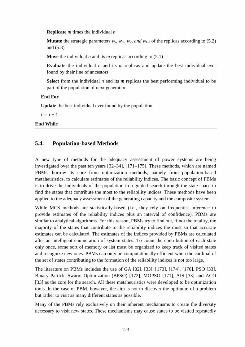
123

Replicate m times the individual n

Mutate the strategic parameters wi, wm, wc, and wGb of the replicas according to (5.2) and (5.3)

Move the individual n and its m replicas according to (5.1)

Evaluate the individual n and its m replicas and update the best individual ever found by their line of ancestors

Select from the individual n and its m replicas the best performing individual to be part of the population of next generation

End For

Update the best individual ever found by the population

t := t + 1

End While

5.4. Population-based Methods

A new type of methods for the adequacy assessment of power systems are being investigated over the past ten years [32–34], [171–175]. These methods, which are named PBMs, borrow its core from optimization methods, namely from population-based metaheuristics, to calculate estimates of the reliability indices. The basic concept of PBMs is to drive the individuals of the population in a guided search through the state space to find the states that contribute the most to the reliability indices. These methods have been applied to the adequacy assessment of the generating capacity and the composite system.

While MCS methods are statistically-based (i.e., they rely on frequentist inference to provide estimates of the reliability indices plus an interval of confidence), PBMs are similar to analytical algorithms. For this reason, PBMs try to find out, if not the totality, the majority of the states that contribute to the reliability indices the most so that accurate estimates can be calculated. The estimates of the indices provided by PBMs are calculated after an intelligent enumeration of system states. To count the contribution of each state only once, some sort of memory or list must be organized to keep track of visited states and recognize new ones. PBMs can only be computationally efficient when the cardinal of the set of states contributing to the formation of the reliability indices is not too large.

The literature on PBMs includes the use of GA [32], [33], [173], [174], [176], PSO [33], Binary Particle Swarm Optimization (BPSO) [172], MOPSO [171], AIS [33] and ACO [33] as the core for the search. All these metaheuristics were developed to be optimization tools. In the case of PBM, however, the aim is not to discover the optimum of a problem but rather to visit as many different states as possible.

Many of the PBMs rely exclusively on their inherent mechanisms to create the diversity necessary to visit new states. These mechanisms may cause states to be visited repeatedly

124

before new states are discovered. Moreover, the number of repetitions starts to grow considerably when the PBM has already visited a considerable number of states. This leads to the concepts of accuracy and efficiency of the PBM. Accuracy measures how good the estimates of the reliability indices provided by the PBMs are, while efficiency measures the ratio of different states visited against the total number of states visited. Hence, low efficiency indicates that many repetitions are being made instead of visits to new states. If there are many repeated visits before new states are discovered, the PBM can require many generations to provide accurate estimates of the reliability indices, or, in the worst case scenario, the search can be suddenly stopped since the PBM might wrongly assume that all states that contribute to the formation of the indices have already been found.

The number of repetitions can be reduced if PBMs are equipped with additional mechanisms for creating diversity. Bearing this in mind, the work in [34], which is based on the EPSO metaheuristic, introduced the use of innovative searching techniques4 to spread the population over the space. As a result, not only the efficiency of the PBM was improved, i.e., an increase of the ratio of different states visited against the total number of states visited was confirmed, but also its accuracy, i.e., better estimates of the reliability indices for the same computational effort were obtained. The following section presents the basics of PBMs.

5.4.1. Estimating Reliability Indices using Population-based Methods

The process of estimating reliability indices via PBMs consists of two phases: a search phase and an indices calculation phase. The search phase uses the individuals of the population to search for the highest possible number of different and high probability states with insufficient capacity to supply the peak load. During this phase there is neither a sense of sequential order nor time-dependency. The peak load level is used to guarantee a large collection of states that are likely to have loss of load for lower load levels.

The states that fulfill the aforementioned criteria are saved in a list. This list is used to avoid saving states that have already been visited and to help recognize new ones. Actually, the states are only saved if their probability is greater than or equal to a threshold. This necessary condition aims to keep the size of list within reasonable limits and, as a consequence, to control the computational effort associated with searching and storing states.

Generally, the stopping criterion of the search phase of PBMs can be based on a maximum allowed number of generations or on the “stability” of a given annualized reliability index. Taking the annualized EPNS as an example, the latter stopping criterion can be mathematically formulated as

εMAX

MAX

Nk

Nkk ≤−−

−

EPNSEPNSEPNS

(5.5)

4 These spreading mechanisms are normally tailored-made for the metaheuristic acting as core of the PBM.

125

where k is the current generation, NMAX is the maximum number of generations without

“significant improvement” on the estimate of the annualized EPNS, and ε is the tolerance for the “significant improvement”. The annualized EPNS can be calculated using (2.5) by accumulating the contribution of the states in the list.

Note that PBMs do no guarantee that the estimate of the annualized EPNS at the end of the search process is accurate. This observation is justified by the minimum probability that the states must have to be saved in the list. For that reason, the reliability indices estimated by PBMs always underestimate their correct value. Figure 5.2 illustrates the typical evolution of the annualized EPNS during the search process. Note the gap between the accurate value of this index and its estimate calculated by the PBM.

Figure 5.2 – Formation of the annualized EPNS during the search phase.

The second phase of PBMs consists of the computation of the estimates of the annual reliability indices. This process is done by confronting the states saved in the list with the annual load curve. According to this process, the estimate of the annual LOLE can be calculated as

∑∑= ∈

=T

i Sj

j

i

p1

LOLE (5.6)

where i is the i-th hour yearly load curve, T is the total number of hours of the year, Si is the subset of whole set of states S in the list without enough capacity to supply the load of the hour i, and pj is the probability of the state j.

Conversely, the EENS can be estimated as

∑∑= ∈

∆×=T

i Sj

ijj

i

Pp1

EENS (5.7)

where ∆Pj is the loss of load of the state j for the hour i.

Generation

Accurate

EPNS

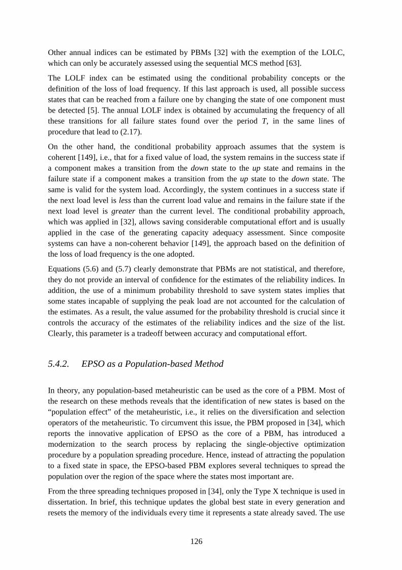
126

Other annual indices can be estimated by PBMs [32] with the exemption of the LOLC, which can only be accurately assessed using the sequential MCS method [63].

The LOLF index can be estimated using the conditional probability concepts or the definition of the loss of load frequency. If this last approach is used, all possible success states that can be reached from a failure one by changing the state of one component must be detected [5]. The annual LOLF index is obtained by accumulating the frequency of all these transitions for all failure states found over the period T, in the same lines of procedure that lead to (2.17).

On the other hand, the conditional probability approach assumes that the system is coherent [149], i.e., that for a fixed value of load, the system remains in the success state if a component makes a transition from the down state to the up state and remains in the failure state if a component makes a transition from the up state to the down state. The same is valid for the system load. Accordingly, the system continues in a success state if the next load level is less than the current load value and remains in the failure state if the next load level is greater than the current level. The conditional probability approach, which was applied in [32], allows saving considerable computational effort and is usually applied in the case of the generating capacity adequacy assessment. Since composite systems can have a non-coherent behavior [149], the approach based on the definition of the loss of load frequency is the one adopted.

Equations (5.6) and (5.7) clearly demonstrate that PBMs are not statistical, and therefore, they do not provide an interval of confidence for the estimates of the reliability indices. In addition, the use of a minimum probability threshold to save system states implies that some states incapable of supplying the peak load are not accounted for the calculation of the estimates. As a result, the value assumed for the probability threshold is crucial since it controls the accuracy of the estimates of the reliability indices and the size of the list. Clearly, this parameter is a tradeoff between accuracy and computational effort.

5.4.2. EPSO as a Population-based Method

In theory, any population-based metaheuristic can be used as the core of a PBM. Most of the research on these methods reveals that the identification of new states is based on the “population effect” of the metaheuristic, i.e., it relies on the diversification and selection operators of the metaheuristic. To circumvent this issue, the PBM proposed in [34], which reports the innovative application of EPSO as the core of a PBM, has introduced a modernization to the search process by replacing the single-objective optimization procedure by a population spreading procedure. Hence, instead of attracting the population to a fixed state in space, the EPSO-based PBM explores several techniques to spread the population over the region of the space where the states most important are.

From the three spreading techniques proposed in [34], only the Type X technique is used in dissertation. In brief, this technique updates the global best state in every generation and resets the memory of the individuals every time it represents a state already saved. The use

127

of just one spreading technique aims to simplify the implementation of the EPSO-based PBM and to make its execution as fast as possible.

It is worth remarking that the EPSO metaheuristic is designed for real-valued spaces. However, the system states in power system adequacy assessment are vectors whose entries follow a Bernoulli distribution. In other words, a system state X is a binary-vector. To obtain a binary-vector from a real-vector, a rounding procedure must be performed. The rounding procedure must be carefully chosen so that 0 and 1 have equal probability of being attained. The following figure illustrates the rounding scheme of the EPSO-based PBM. Note that the entry xi of X is limited to the interval {xi ∈ ℝ | -0.5 < xi < 1.5} to avoid obtaining -1 and 2.

Figure 5.3 – Illustration of the rounding scheme of the EPSO-based PBM.

The following pseudocode describes the EPSO-based PBM used in this dissertation. Since the purpose of this method is to obtain the list of states and not to calculate the estimates for the annual reliability indices, the phase where those calculations are made is not included in this pseudocode.

Pseudocode 5: Evolutionary Particle Swarm Optimization as Search Method

Initialize a population P of n individuals, which can be based on random or heuristic processes, the number of replications per individual m, the communication probability P, the mutation rate τ, the probability threshold pmin, the maximum tolerance ε for the improvement of the annualized index selected to gauge the convergence, the maximum number of generations NMAX without “significant” improvement on the estimate of the annualized index selected and three constants M1, M2 and M3 such that M1 >> M2 >> M3 (typically, M1 ≤ 1×10-100)

Evaluate all individuals according to PA6 and update the best individual ever found by their line of ancestors

Find the best individual in the current population as use it as the best individual ever found

t = 1

While the convergence criteria, which can be based on a maximum allowed number of generations or the criterion represented by (5.5), is not satisfied

For all n individuals of the population of the current generation t

Replicate m times the individual n

Mutate the strategic parameters wi, wm, wc, and wGb of all replicas according to (5.2) and (5.3)

Move individual n and its replicas according to (5.1)

128

Evaluate individual n and its replicas according to PA6 and update the best individual ever found by their line of ancestors

Select from the individual n and its m replicas the best performing individual to be part of the population of next generation

Update the estimate of the annualized index selected to gauge the convergence using (5.5) or (5.6)

End For

Find the best individual in the current population as use it as the best individual ever found

t := t + 1

End While

The performance of an individual must take into account if the state represented by it has already been saved. Accordingly, the fitness of individuals that represent states eligible to enter the list is assumed equal to the multiplication of the probability of that state with the respective loss of load. On the contrary, the individuals that represent states already saved or states that do not fulfill the criteria to enter the list must be set a low fitness value. According to this, the following pseudocode for the computation of the fitness of the individuals is presented:

Pseudocode 6: Evaluation of an Individual

Round the current position of the individual to obtain the equivalent state

Calculate the probability of the state

If the probability is greater than or equal to pmin

Then If the state is not contained in the list

Evaluate the state considering the peak load to detect if there is load loss

If there is load loss

Then add the state to the list and assign the fitness of the individual the product of its probability with the loss of load

Else assign M1 as the fitness of the individual

End If

Else assign M2 as the fitness of the individual

End If

Else assign M3 as the fitness of the individual

End If

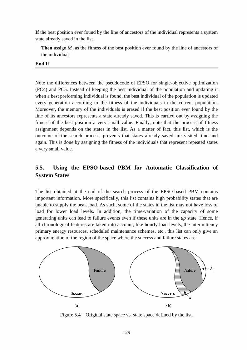
129

If the best position ever found by the line of ancestors of the individual represents a system state already saved in the list

Then assign M3 as the fitness of the best position ever found by the line of ancestors of the individual

End If

Note the differences between the pseudocode of EPSO for single-objective optimization (PC4) and PC5. Instead of keeping the best individual of the population and updating it when a best preforming individual is found, the best individual of the population is updated every generation according to the fitness of the individuals in the current population. Moreover, the memory of the individuals is erased if the best position ever found by the line of its ancestors represents a state already saved. This is carried out by assigning the fitness of the best position a very small value. Finally, note that the process of fitness assignment depends on the states in the list. As a matter of fact, this list, which is the outcome of the search process, prevents that states already saved are visited time and again. This is done by assigning the fitness of the individuals that represent repeated states a very small value.

5.5. Using the EPSO-based PBM for Automatic Classification of System States

The list obtained at the end of the search process of the EPSO-based PBM contains important information. More specifically, this list contains high probability states that are unable to supply the peak load. As such, some of the states in the list may not have loss of load for lower load levels. In addition, the time-variation of the capacity of some generating units can lead to failure events even if these units are in the up state. Hence, if all chronological features are taken into account, like hourly load levels, the intermittency primary energy resources, scheduled maintenance schemes, etc., this list can only give an approximation of the region of the space where the success and failure states are.

Figure 5.4 – Original state space vs. state space defined by the list.

130

Figure 5.4 was created to help explain the observations of the last paragraph. This figure depicts a straightforward representation of the original state space, which contains the actual success and failure states when all chronological issues are considered (Figure 5.4(a)). In addition, this figure has the approximate representation of the state space using the information in the list provided by the EPSO-based PBM (Figure 5.4(b)).

According to Figure 5.4(b), the list of states can be used to divide the space into four zones: two zones containing potential success states and two zones containing potential failure states. The zone containing potential success states encompasses the subzone where the actual success states are and a subzone that theoretically has success states but in fact contains failure states. The latter subzone is represented in Figure 5.4(b) by A2. The size of this subzone is closely related to the probability threshold, pmin, of the EPSO-based PBM. Recall that this probability threshold is used to avoid saving the states that have a probability inferior to a pre-set value in the list even if they have loss of load. If the number of states within A2 is sufficiently large, the accuracy of the estimates of the reliability indices might be severely compromised. Nevertheless, the size of A2 can be easily controlled by selecting an appropriate pmin. Recall that this threshold plays an important role on the CPU time of the EPSO-based PBM since it controls the size of the list.

The zone containing potential failure states encloses the subzone where the actual failure states are and a subzone that ideally has failure states but, in fact, contains success states. The latter subzone is represented in Figure 5.4(b) by A1. The reason why this subzone exits is related to assumptions made by the PBM. Since the search process only uses the peak load level and overlooks the representation of the time-dependent issues, some states saved in the list might not have loss of load for lower load levels. Unfortunately, the size of A1 cannot be easily controlled. The use of approximate representations for the chronology of the system in the search phase of the PBM can help mitigate this problem. Note that the accuracy of the estimates of the reliability indices will not be affected by A1.

5.6. Generation, Transmission and Composite States

Section 2.8.2.2 has shown that the sequential MCS method advances through time by altering the state of only one system component at a time. Accordingly, system states can be formed by sequentially combining the states of its components. Consider, for instance, the example depicted in Figure 2.4. According to this figure, the system load experiences a transition every hour whereas the generating capacity can remain unchanged for longer periods of time due to the relative duration of the up and down states of the generating units against the fixed duration of the load levels.

Now, assume that the period of time where the state of all generating units remains unchanged defines a Generation State (GS). Being this the case, a considerable number of system states5 can occur during a GS. The number of system states occurred depends on

5 A system state includes the state of the system components and the load state.

131

the duration of the GS and the duration of the load levels. For instance, Figure 2.4 shows that there are 8 system states during the first GS. This figure also shows that none of these eight system states have loss of load. Hence, if some automatic procedure could detect at the beginning of the GS that the 8 system states would be success, eight compositions and evaluations would have been avoided.

Undoubtedly, the classification of GS can be implemented using machine learning algorithms. Equally, this classification procedure can be straightforwardly implemented by using a list of GSs that fail to supply the peak load. Therefore, this dissertation proposes the use of the information contained in the list created by the EPSO-based PBM to decide at the beginning of every GS sampled by the sequential MCS method whether it should proceed to composition and evaluation. Naturally, the highest gains in CPU time are expected when the number of success system states is considerably smaller than the number of failure system states and when the average duration of the GSs is greater than the average duration of system states.

The GS concept can be generalized for the case of the components of the transmission system. Accordingly, a Transmission State (TS) is defined by the period of time where the state of all transmission circuits remains unchanged. Likewise, a Composite State (CS) comprises the period where the state of the generating units and transmission circuits is unaltered. Hence, a CS aggregates only one GS and one TS. Note that GSs, TSs and CSs are defined by the availability of the system components and not by the capacity they have when they are in the up or down states.

Figure 5.5 – Generation, transmission and composite states.

Figure 5.5 was created to help understand the GS, TS and CS concepts. This figure represents transitions between the up and down states that can occur in a system composed of two generators, G1 and G2, and of one transmission circuit, T1. This figure shows that there are three GSs. The first one starts at the instant t = 0+ and ends at t = t1. The second GS begins at t = t1

+ and ends at t = t2. The beginning of the last GS is at t = t2+ while its end

takes place when G1 or G2 return to the up state. As for the case of TSs, one can see from Figure 5.5 that there are only two, which correspond to the up and down states of the circuit T1. Lastly, this figure reveals that a when one of the three components of the system change its respective state, a new CS begins. Accordingly, there are 4 CSs. Note that a system state comprises the state of all system components, including the state of the system

Up

Down

Up

Down

Up

Down

t1

G1

G2

T1

t2 t3 t40 t

132

load. Since the system load was not included in this example, there are no system states in Figure 5.5.

5.6.1. Representation of Generation, Transmission and Composite States as Individuals of Population-based Methods

The straightforward way to represent GSs, TSs, or CSs as individuals of the EPSO-based PBM is to use the scheme proposed in subsection 5.4.2. More specifically, the up and down states of the components of the system can be represented by using a real-vector, which, after a rounding procedure, becomes a binary-vector. Depending on the number of components, this straightforward representation can result in high-dimensional individuals. Many authors have reported that, as the dimension of the individuals grows, the ability of the metaheuristics to provide acceptable solutions in a reasonable length of time decreases in a way that this fact has been coined as the curse of dimensionality [178]. To avoid high-dimensional individuals, the particularities of the system under evaluation can be cleverly used. The fact that some components are equal and iid can be taken advantage of to create low-dimensional individuals.

Consider, for instance, a system composed of two iid generating units with 10 MW of capacity and a single load level. This system has 22 = 4 system states: one with 20 MW of generating capacity, two with 10 MW and one with 0 MW. The number of state evaluations needed to determine the reliability indices is 4. Under the representation proposed in the subsection 5.4.2, an individual of the EPSO-based PBM would have a size of 2. Now, assume that the number of states with equal capacity can be easily computed. In this case, one needs only to find one of the two 10 MW system states to determine their contribution to the reliability indices. Accordingly, the size of the individual can be reduced from 2 to 1 and the dimension of the search space from 4 to 3 since there is only one group of iid generators with equal capacity. Naturally, the reduction achieved depends on the characteristics of the system under evaluation. In a system where all components are different, there is no reduction.

From what has been said, one can define a GS as an integer-vector whose entries contain the number of equal and iid generating units in the up state. Equal generating units are all those that have the same generating capacity and rely on the same primary energy resource. Note that the probability of a GS is different from the probability of a system state. In fact, a GS includes many equal states, i.e., states with equal generating capacity and equal probability.

Take, for instance, the case of the IEEE-RTS 79. As Table 4.1 shows, this system has 9 different groups of equal and iid generating units. Hence, for a system with NC groups of equal and iid generating units, the number of equal states nS included in a GS is given by

∏=

=NC

i i

iS

k

nn

1

(5.8)

133

where ni is the total number of units of group i and ki is the number of units of group i in the up state. In simple terms, the probability of a GS results from accumulating the probability of all nS equal states represented by it.

Like a GS, a TS is also an integer-vector. However, the entries of this integer-vector contain the number of equal and iid transmission circuits in the up state. Equal transmission circuits have the same electrical parameters, the same capacity and connect two adjacent buses. Like in the case of GSs, the probability of a TS is the sum of the probability of all equal states represented by it.

A CS aggregates equal and iid generating units as well as equal and iid transmission lines. The concept of equal transmission lines is along the same lines as the concept defined for the TSs. Conversely, the concept of equal generating units is different from the concept proposed for the GSs since the location of the units in the transmission system must be taken into account. Hence, equal generating units in a CS are all those that have an equal generating capacity, use the same primary energy resource and are connected at the same bus. Two different nomenclatures are proposed to help distinguish the GS defined previously from the GS aggregated by CSs. As a result, the former GS is named as GS-1 whereas the latter is denoted as GS-2. Similarly to the case of GSs-1 and TSs, the probability of a CS accounts for the contribution of all equal nS states aggregated by it.

To clarify the concepts of GS-1, TS and CS take the example of the IEEE-RTS 79 [91]. This system has 32 generating units, 33 transmission lines and 5 transformers. Thus, a system state of the IEEE-RTS 79 contains 70 entries and an extra entry for the system load. Moreover, nine of the 32 generating units of the IEEE-RTS 79 are equal and iid according to the definition of a GS-1. Hence, the size of a GS-1 is 9. In turn, the inspection of the transmission circuits of this system reveals 7 are iid and equal. Thus, the size of a TS is 32. Finally, if the assumptions of CSs are followed, it is possible to detect 32 equal and iid transmission circuits and 14 equal and iid generating units (note that some of the 9 equal generating units detected in the case of GSs-1 are not equal anymore under the assumptions of GSs-2). Thus, the size of a CS is 14 + 32 = 46, which is smaller than the size of a system state (70 +1).

5.6.2. Encoding Generation, Transmission and Composite States

The list created by the EPSO-based PBM can include GSs-1, TSs or CSs (i.e., a GSs-2 + TSs). This list must be implemented using a fast access memory. One way to assure this is to use the hash table [177] concept of the JAVA language. In simple terms, a hash table is a data structure that implements an associative relation between keys and buckets for data storage. This type of data structure can be used for database indexing. This type of application aims to speed up the retrieval of data at the cost of a slower writing, updating or deleting of data operations.

To fulfill the requirements of the list of states, one can use the hash table to store the individuals of the EPSO-based PBM in its buckets. On the other hand, its keys can be used

134

to identify GSs, TSs or CSs, remaining the buckets completely empty to reduce the storage requirements of the hash table. This demands for an encoding process that guarantees a unique code for every GS-1, TS and GS (GSs-2 + TSs). Moreover, the codes created must be in a format that can be used as keys of the hash table.

Bearing this in mind, the encoding process of GSs-1 used in this dissertation consists of creating a sequence of characters that represent the number of equal and iid generating units in the up state, i.e., the integer-vectors are converted into strings. These strings are used as a key of the hash table.

TSs are also encoded by strings, which, unlike the GSs-1, contain the identification of the transmission circuits in the down state. When a TS is repeated, all equal states are converted into strings, which are then included in the hash table. The reason why TSs have a dissimilar representation from GSs is twofold. First of all, transmission circuits fail less than generating units. Second, the number of equal transmission circuits is considerably smaller than the number of generating units. Hence, if the key proposed for GSs-1 was adopted for TSs, the size of the resulting key would be equal to the number of equal and iid circuits in the system while containing the same information as the encoding process proposed.

Finally, the encoding process of the CSs consists in the aggregation of the equal and iid generating units in the up state and the identification of the transmission circuits in the down state in a single string. Note that the term equal generating units in the last sentence refers to the definition adopted for the CSs (see section 5.6.1).When a CS represents more than one state, all repetitions are converted into respective strings and included in the hash table.

5.7. Generating Capacity Adequacy Assessment using the EPSO-based PBM as Automatic Classification System

This section reports results from the application of an EPSO-based PBM to enhance time-efficiency of the sequential MCS method for the generating capacity adequacy assessment. The methodology proposed consists of two phases. The first phase, which is named Phase A, consists of using the EPSO-based PBM to search for GSs-1. A GSs-1 is included in the list if its generating capacity is insufficient to supply the system load and if its probability is greater than or equal to a given threshold.

The second phase, which is called Phase B, uses the sequential MCS method to estimate the annual reliability indices. While Phase A is based on PC5 and PA6, the core of Phase B is the sequential MCS method proposed in section 2.9.2. Figure 5.6 illustrates the structure of the methodology proposed. This figure puts a special emphasis on the classification process of Phase B. According to Figure 5.6, the GSs-1 sampled only proceed to the state composition and evaluation step if they are in the list. Moreover, a GS-1 can be allowed to advance to composition and evaluation if the last system state evaluated is failure. This auxiliary criterion was included in the methodology to avoid the disruption of the loss of

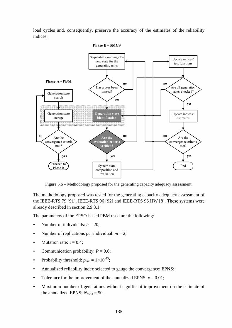
135

load cycles and, consequently, preserve the accuracy of the estimates of the reliability indices.

Figure 5.6 – Methodology proposed for the generating capacity adequacy assessment.

The methodology proposed was tested for the generating capacity adequacy assessment of the IEEE-RTS 79 [91], IEEE-RTS 96 [92] and IEEE-RTS 96 HW [8]. These systems were already described in section 2.9.3.1.

The parameters of the EPSO-based PBM used are the following:

• Number of individuals: n = 20;

• Number of replications per individual: m = 2;

• Mutation rate: τ = 0.4;

• Communication probability: P = 0.6;

• Probability threshold: pmin = 1×10-15;

• Annualized reliability index selected to gauge the convergence: EPNS;

• Tolerance for the improvement of the annualized EPNS: ε = 0.01;

• Maximum number of generations without significant improvement on the estimate of the annualized EPNS: NMAX = 50.

Generation state

search

Generation state

storage

Are the

convergence criteria

met?

Phase A - PBM

yes

no

Proceed to

Phase B

Sequential sampling of a

new state for the

generating units

Generation state

identification

Are the

evaluation criteria

verified?

Has a year been

passed?

System state

composition and

evaluation

Update indices’

test functions

Are all generation

states checked?

Update indices’

estimates

Are the

convergence criteria

met?

End

yes

yes

no

no no

yes

yes

no

Phase B - SMCS

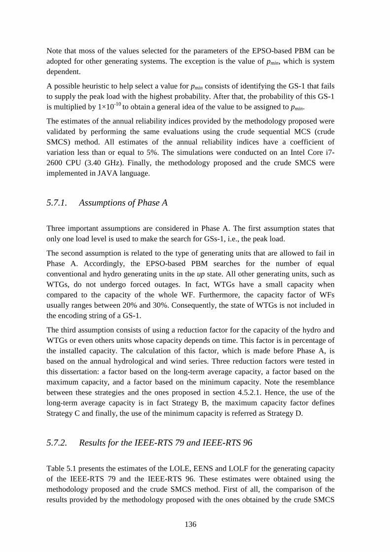
136

Note that moss of the values selected for the parameters of the EPSO-based PBM can be adopted for other generating systems. The exception is the value of pmin, which is system dependent.

A possible heuristic to help select a value for pmin consists of identifying the GS-1 that fails to supply the peak load with the highest probability. After that, the probability of this GS-1 is multiplied by 1×10-10 to obtain a general idea of the value to be assigned to pmin.

The estimates of the annual reliability indices provided by the methodology proposed were validated by performing the same evaluations using the crude sequential MCS (crude SMCS) method. All estimates of the annual reliability indices have a coefficient of variation less than or equal to 5%. The simulations were conducted on an Intel Core i7-2600 CPU (3.40 GHz). Finally, the methodology proposed and the crude SMCS were implemented in JAVA language.

5.7.1. Assumptions of Phase A

Three important assumptions are considered in Phase A. The first assumption states that only one load level is used to make the search for GSs-1, i.e., the peak load.

The second assumption is related to the type of generating units that are allowed to fail in Phase A. Accordingly, the EPSO-based PBM searches for the number of equal conventional and hydro generating units in the up state. All other generating units, such as WTGs, do not undergo forced outages. In fact, WTGs have a small capacity when compared to the capacity of the whole WF. Furthermore, the capacity factor of WFs usually ranges between 20% and 30%. Consequently, the state of WTGs is not included in the encoding string of a GS-1.

The third assumption consists of using a reduction factor for the capacity of the hydro and WTGs or even others units whose capacity depends on time. This factor is in percentage of the installed capacity. The calculation of this factor, which is made before Phase A, is based on the annual hydrological and wind series. Three reduction factors were tested in this dissertation: a factor based on the long-term average capacity, a factor based on the maximum capacity, and a factor based on the minimum capacity. Note the resemblance between these strategies and the ones proposed in section 4.5.2.1. Hence, the use of the long-term average capacity is in fact Strategy B, the maximum capacity factor defines Strategy C and finally, the use of the minimum capacity is referred as Strategy D.

5.7.2. Results for the IEEE-RTS 79 and IEEE-RTS 96

Table 5.1 presents the estimates of the LOLE, EENS and LOLF for the generating capacity of the IEEE-RTS 79 and the IEEE-RTS 96. These estimates were obtained using the methodology proposed and the crude SMCS method. First of all, the comparison of the results provided by the methodology proposed with the ones obtained by the crude SMCS

137

method shows that the two alternatives provide similar estimates. As a matter of fact, the relative error of the LOLE estimate provided by the methodology proposed is 0.084% in the case of the IEEE-RTS 79 and 4.3% for the IEEE-RTS 96. This result proves that the methodology proposed can accurately sort out the GSs-1 that contain system states with loss of load from those that do not.

Table 5.1 – Results of the methodology proposed for the generating capacity of the IEEE-RTS 79 and IEEE-RTS 96.

IEEE-RTS 79 IEEE-RTS 96

Methodology Proposed

Crude SMCS

Methodology Proposed

Crude SMCS

LOLE (h/yr) 9.542 9.550 0.1307 0.1366 EENS (MWh/yr) 1267.20 1266.90 22.58 23.81 LOLF (occ./yr) 2.027 2.029 0.05017 0.05198

Years Simulated 3143 3140 65 674 64 063 System States

Composed and Evaluated 8 123 787 28 883 137 12 257 445 648 547 765

Total CPU Time (min) 0.25 0.63 8.37 40.62 Phase A CPU Time (min) 1.96×10-2 - 0.15 -

Average CPU Time Required by Phase B

to Evaluate a Year (ms) 3.09 10.89 0.74 31.14

Table 5.1 also shows that an inferior number of system states are composed and evaluated if the methodology proposed is used instead of the crude SMCS method. For the case of the IEEE-RTS 79, the methodology proposed required only 28.13% of the system states composed and evaluated by the crude SMCS method. The similar analysis for the IEEE-RTS 96 reveals that only 1.89% of the compositions and evaluations are required.

The composition and evaluation of less system states can result in significant savings in CPU time if the classification process and Phase A are time-efficient. In view of that, Table 5.1 reports that the time lost in Phase A is not significant as compared with the CPU time required by the crude SMCS method.

Moreover, the average time required to evaluate a synthetically created year is considerably reduced when GSs-1 are automatic classified using the methodology proposed. Accordingly, the use of the list of GSs-1 results in an average speed up of the composition and evaluation of the GSs-1 in a year of simulation 3.52 for the case of the IEEE-RTS 79 and 42.08 for the IEEE-RTS 96. Hoverer, since the number of years simulated and the dimension of the generating systems of the IEEE-RTS 79 and IEEE-RTS 96 are different, the same speed ups are not reflected in the total CPU time. As a matter of fact, the speed up obtained for the IEEE-RTS 79 is 2.52 and 4.85 for the IEEE-RTS 96. This shows that, for the adequacy assessment of the generating system, the composition and evaluation of system states are not the procedures that demand the most time.

Note that the speed ups obtained are not caused by the reduction of the variance of the estimators. Being this the case, it is expected that the probability distributions provided by the methodology proposed are at least similar to those obtained by the crude SMCS

138

method. Accordingly, the cdf of the LOLE index of the IEEE-RTS 79 and IEEE-RTS 96 was obtained by the methodology proposed and the crude SMCS method. The respective distributions are depicted in Figure 5.7 and Figure 5.8.

Figure 5.7 – Cdf of the LOLE for the IEEE-RTS 79.

Figure 5.8 – Cdf of the LOLE for the IEEE-RTS 96.

The visual inspection of the last two figures reveals that the cdfs provided by both methods are practically superimposed. As a matter of fact, the greatest dissimilarities were observed for the case of the IEEE-RTS 96, which is precisely the generating system where the estimate of the LOLE index has the greatest relative error. As a result, the methodology proposed can only provide accurate probability distributions when the error of the estimates of the reliability indices is negligible.

The accuracy of the methodology proposed was also investigated. For this purpose, statistics were collected during Phase A and Phase B for the adequacy assessment of the

9898.298.498.698.8

9999.299.499.699.8100

0 5 10 15 20 25 30 35 40

Cum

ulat

ive

Pro

babi

lity

(%)

LOLE (h/yr)

Crude SMCS Proposed Methodology

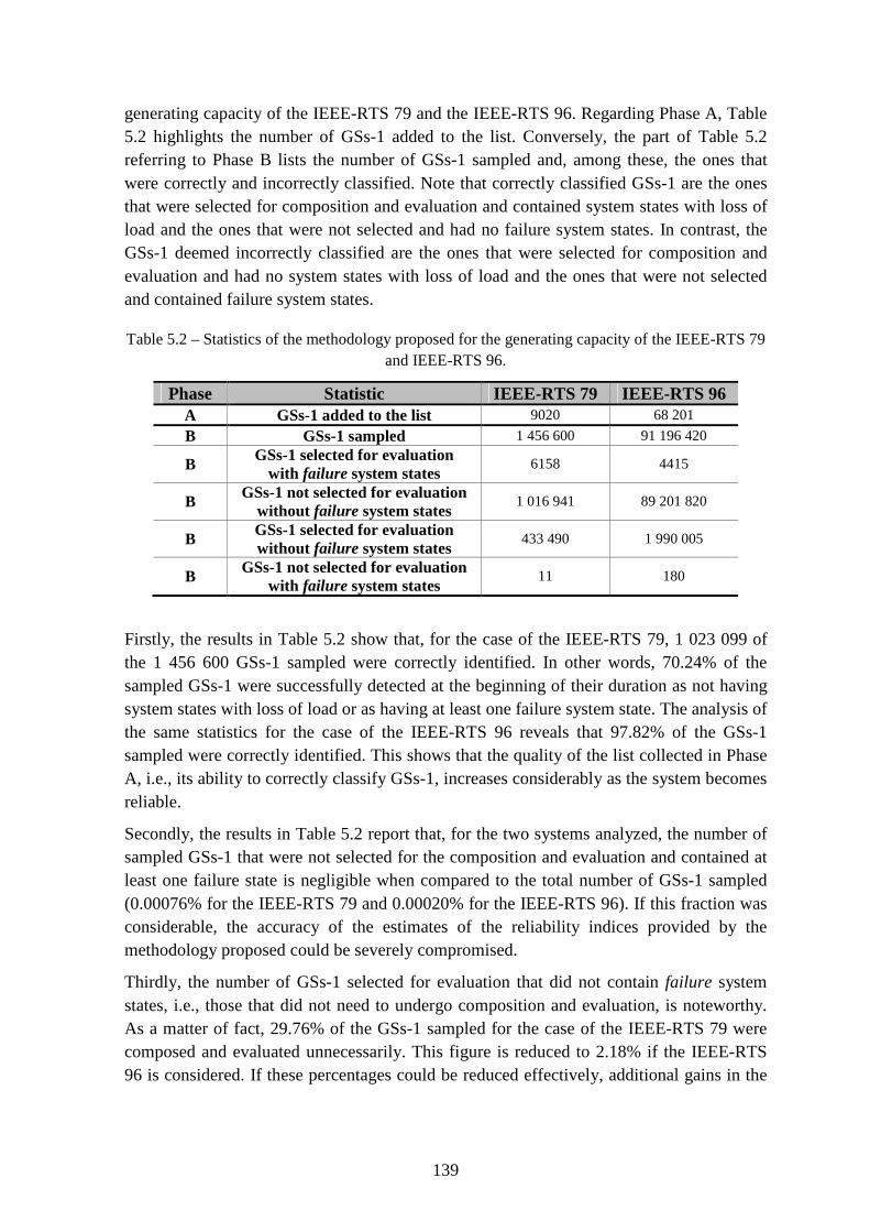
139

generating capacity of the IEEE-RTS 79 and the IEEE-RTS 96. Regarding Phase A, Table 5.2 highlights the number of GSs-1 added to the list. Conversely, the part of Table 5.2 referring to Phase B lists the number of GSs-1 sampled and, among these, the ones that were correctly and incorrectly classified. Note that correctly classified GSs-1 are the ones that were selected for composition and evaluation and contained system states with loss of load and the ones that were not selected and had no failure system states. In contrast, the GSs-1 deemed incorrectly classified are the ones that were selected for composition and evaluation and had no system states with loss of load and the ones that were not selected and contained failure system states.

Table 5.2 – Statistics of the methodology proposed for the generating capacity of the IEEE-RTS 79 and IEEE-RTS 96.

Phase Statistic IEEE-RTS 79 IEEE-RTS 96 A GSs-1 added to the list 9020 68 201

B GSs-1 sampled 1 456 600 91 196 420

B GSs-1 selected for evaluation

with failure system states 6158 4415

B GSs-1 not selected for evaluation without failure system states

1 016 941 89 201 820

B GSs-1 selected for evaluation without failure system states

433 490 1 990 005

B GSs-1 not selected for evaluation with failure system states

11 180

Firstly, the results in Table 5.2 show that, for the case of the IEEE-RTS 79, 1 023 099 of the 1 456 600 GSs-1 sampled were correctly identified. In other words, 70.24% of the sampled GSs-1 were successfully detected at the beginning of their duration as not having system states with loss of load or as having at least one failure system state. The analysis of the same statistics for the case of the IEEE-RTS 96 reveals that 97.82% of the GSs-1 sampled were correctly identified. This shows that the quality of the list collected in Phase A, i.e., its ability to correctly classify GSs-1, increases considerably as the system becomes reliable.

Secondly, the results in Table 5.2 report that, for the two systems analyzed, the number of sampled GSs-1 that were not selected for the composition and evaluation and contained at least one failure state is negligible when compared to the total number of GSs-1 sampled (0.00076% for the IEEE-RTS 79 and 0.00020% for the IEEE-RTS 96). If this fraction was considerable, the accuracy of the estimates of the reliability indices provided by the methodology proposed could be severely compromised.

Thirdly, the number of GSs-1 selected for evaluation that did not contain failure system states, i.e., those that did not need to undergo composition and evaluation, is noteworthy. As a matter of fact, 29.76% of the GSs-1 sampled for the case of the IEEE-RTS 79 were composed and evaluated unnecessarily. This figure is reduced to 2.18% if the IEEE-RTS 96 is considered. If these percentages could be reduced effectively, additional gains in the

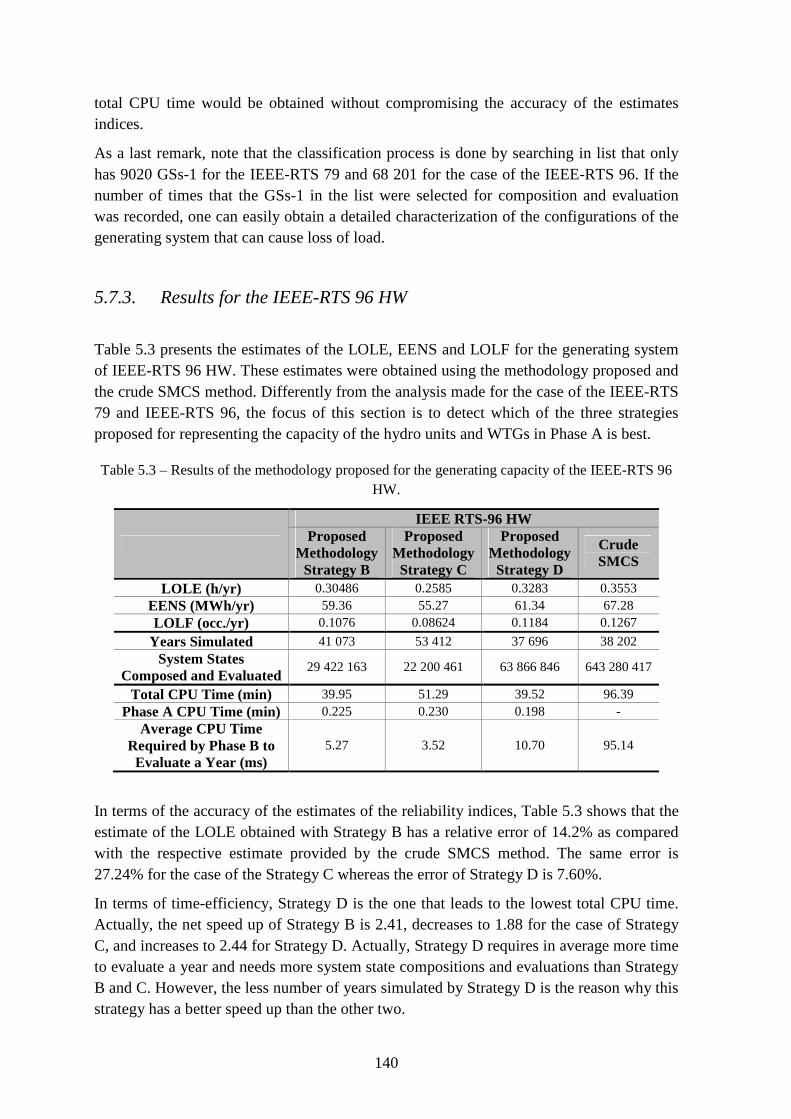
140

total CPU time would be obtained without compromising the accuracy of the estimates indices.

As a last remark, note that the classification process is done by searching in list that only has 9020 GSs-1 for the IEEE-RTS 79 and 68 201 for the case of the IEEE-RTS 96. If the number of times that the GSs-1 in the list were selected for composition and evaluation was recorded, one can easily obtain a detailed characterization of the configurations of the generating system that can cause loss of load.

5.7.3. Results for the IEEE-RTS 96 HW

Table 5.3 presents the estimates of the LOLE, EENS and LOLF for the generating system of IEEE-RTS 96 HW. These estimates were obtained using the methodology proposed and the crude SMCS method. Differently from the analysis made for the case of the IEEE-RTS 79 and IEEE-RTS 96, the focus of this section is to detect which of the three strategies proposed for representing the capacity of the hydro units and WTGs in Phase A is best.

Table 5.3 – Results of the methodology proposed for the generating capacity of the IEEE-RTS 96 HW.

IEEE RTS-96 HW Proposed

Methodology Strategy B

Proposed Methodology Strategy C

Proposed Methodology Strategy D

Crude SMCS

LOLE (h/yr) 0.30486 0.2585 0.3283 0.3553 EENS (MWh/yr) 59.36 55.27 61.34 67.28 LOLF (occ./yr) 0.1076 0.08624 0.1184 0.1267

Years Simulated 41 073 53 412 37 696 38 202 System States

Composed and Evaluated 29 422 163 22 200 461 63 866 846 643 280 417

Total CPU Time (min) 39.95 51.29 39.52 96.39 Phase A CPU Time (min) 0.225 0.230 0.198 -

Average CPU Time Required by Phase B to Evaluate a Year (ms)

5.27 3.52 10.70 95.14

In terms of the accuracy of the estimates of the reliability indices, Table 5.3 shows that the estimate of the LOLE obtained with Strategy B has a relative error of 14.2% as compared with the respective estimate provided by the crude SMCS method. The same error is 27.24% for the case of the Strategy C whereas the error of Strategy D is 7.60%.

In terms of time-efficiency, Strategy D is the one that leads to the lowest total CPU time. Actually, the net speed up of Strategy B is 2.41, decreases to 1.88 for the case of Strategy C, and increases to 2.44 for Strategy D. Actually, Strategy D requires in average more time to evaluate a year and needs more system state compositions and evaluations than Strategy B and C. However, the less number of years simulated by Strategy D is the reason why this strategy has a better speed up than the other two.

141

The accuracy of the three strategies was also investigated. For this purpose, statistics equal to the ones presented in Table 5.2 were collected for strategies B, C and D. These results are shown in Table 5.4.

Table 5.4 – Statistics of the methodology proposed for the generating capacity of the IEEE-RTS 96 HW.

Phase Statistic Strategy B Strategy C Strategy D A GSs-1 added to the list 78 609 71 480 81 453

B GSs-1 sampled 331 869 684 431 555 183 304 577 973

B GSs-1 selected for evaluation with failure system states

16 022 17 382 15 927

B GSs-1 not selected for evaluation without failure system states

317 573 611 420 833 469 273 505 424

B GSs-1 selected for evaluation without failure system states

14 277 607 10 697 527 31 055 381

B GSs-1 not selected for evaluation

with failure system states 2444 6805 1241

As expected, the strategy with the lowest number of GSs-1 that were not selected for composition and evaluation and had failure system states is Strategy D. This same number increases almost to the double for the case of Strategy B and 5.5 times for Strategy C. On the other hand, the comparison of the number of GSs-1 added to the lists shows that Strategy D is the one that collected the highest number of states. In other words, the use of Strategy D has enabled the EPSO-based PBM to cover a wider zone of the space of the GSs-1.

Unfortunately, the greater size of the list of Strategy D makes the composition and evaluation of GSs-1 that had no failure states more frequent. For instance, take the ratio between the number of incorrectly identified GSs-1 against the total number of GSs-1 sampled. This ratio is 4.30% in the case of Strategy B, decreases to 2.48% for Strategy C and increases to 10.20% if Strategy D is used. This result shows that the reduction of the error of the estimates of the indices is at the cost of the deterioration of the accuracy of the classification process.

5.8. Composite System Adequacy Assessment using the EPSO-based PBM as Automatic Classification System

Last section showed how the EPSO-based PBM can be used to speed up the adequacy assessment of the generating capacity via the sequential MCS method. Given the promising results obtained, this section investigates how this methodology can be used for the composite system adequacy assessment. Once again, the idea is to use the list provided by the EPSO-based PBM to help detect automatically the states sampled in Phase B that need composition and evaluation from the ones that do not. To apply the same methodology for the case of the composite system adequacy assessment, the EPSO-based

142

PBM must search for CSs. If, at the beginning of every CSs sampled in Phase B is possible to know whether system states with loss of load will occur, considerable time-efficiency gains can be expected.

Now, consider the CS concept. As shown in Figure 5.5, a CS aggregates one GS and one TS. Accordingly, it is possible to define at least three methodologies to decide if a composite state should be composed and evaluated.

The first methodology, which is named Methodology CSA, consists of encoding the CS as a GSs-1 (see section 5.6.2) and detect if the string is one of the keys of a hash table previously created by the EPSO-based PBM. Accordingly, the GSs-1 are represented by a string with the number of equal and iid generating units in the up state. In the case of this methodology, equal generating units are the ones with equal capacity (GS-1) and not the ones with equal capacity and located at the same bus (GS-2). To account for failure of transmission circuits, the CSs sampled in Phase B are composed and evaluated if they contain a circuit in the down state.

The second methodology, which is called Methodology CSB, is based on encoding separately the GS and the TS included in CSs. Accordingly, every CSs has two strings: one with the equal and iid generating units in the up state and other with the identification of the transmission circuits in the down state. The codification of the GS and the TS is according to what was proposed in section 5.6.2 for the GSs-1 and TSs. Note that there are two lists in this methodology: one of GSs-1 and the other of TSs.

The third and last methodology, which is named Methodology CSC, consists of using the codification of CSs proposed in section 5.6.2. Accordingly, a single string for the codification of the GS-2 and the TS included in the CS is used. Every time a new CS is sampled in Phase B, the corresponding string is searched in a hash table of CSs to decide if composition and evaluation is carried out. The following sections describe the three methodologies proposed in detail and analyze their efficiency for various test systems.

5.8.1. Methodology CSA

The classification of the CSs sampled in Phase B can be approximately done by detecting if the code of its GS is in a list of GSs. To build such list, the transmission circuits are not included in the search phase. Methodology CSA has two advantages:

• The size of the individuals of the EPSO-based PBM is equal to the number of equal capacity and iid generating units (i.e., the code used is the one proposed for GSs-1);

• Only GSs-1 are evaluated in Phase A, i.e., the evaluation of GSs-1 follows the procedure proposed in section 2.9.2.1 for the generating capacity.

In opposition, the disadvantages of Methodology CSA are:

• The CSs sampled in Phase B will be composed and evaluated whenever a transmission circuit is in the down state.

143

Figure 5.9 – Methodology CSA for the composite system adequacy assessment.

The detection of the CSs that need composition and evaluation is based on three criteria. If there are transmission circuits in the down state or if the last system state evaluated has loss of load, the CS proceeds to composition and evaluation. If not, a string is created for the CS under analysis. If this string is one of the keys of the hash table of GSs-1, the CS is composed and evaluated. If not, it is considered that no system states with loss of load occur throughout the duration of the CS.

Figure 5.9 illustrates the sequence of procedures of Methodology CSA.

The three hypotheses proposed in section 5.7.1 for the representation the generating units with time-dependent capacity in Phase A are also adopted by Methodology CSA. Given the results in Table 5.4, which were obtained for the generating system of the IEEE-RTS 96 HW, only Strategy C is effectively used.

Methodology CSA was used to obtain the estimates of the reliability indices of the composite system of the IEEE-RTS 79 [91], the IEEE-RTS 79 HW and the IEEE-MRTS 79 [93]. The IEEE-RTS 79 HW includes yearly series to model the time-dependency of the capacity of the hydro units and WTGs. The IEEE-RTS 79 HW has already been described in section 2.9.3.1. The estimates of the annual reliability indices for the composite system reported in this section have a coefficient of variation less than or equal to 5%. The

Generation state

search

Generation state

storage

Are the

convergence criteria

met?

Phase A - PBM

yes

no

Proceed to

Phase B

Sequential sampling of a

new state for the

generating units and

transmission circuits

Composite state

identification

Are the

evaluation criteria

verified?

Has a year been

passed?

System state

composition and

evaluation

Update indices’

test functions

Are all composite

states checked?

Update indices’

estimates

Are the

convergence criteria

met?

End

yes

yes

no

no no

yes

yes

no

Phase B - SMCS

144

simulations were conducted on an Intel Core i7-2600 CPU (3.40 GHz). The Methodology CSA and the crude SMCS method were implemented in JAVA language.

The value assumed for the parameters of the Phase A are the following:

• Number of individuals: n = 20;

• Number of replications per individual: m = 2;

• Mutation rate: τ = 0.4;

• Communication probability: P = 0.6;

• Probability threshold: pmin = 1×10-15;

• Annualized reliability index selected to gauge the convergence: EPNS;

• Tolerance for the improvement of the annualized EPNS: ε = 0.01;

• Maximum number of generations without significant improvement on the estimate of the annualized EPNS: NMAX = 50.

5.8.1.1. Results for the IEEE-RTS 79 and IEEE-RTS 79 HW

Table 5.5 shows the results of the application of Methodology CSA to the composite system adequacy assessment of the IEEE-RTS 79 and the IEEE-RTS 79 HW. These results include the estimates of the LOLE, EENS and LOLF indices, the number of years simulated, the number of system states evaluated, the total CPU time, the CPU time required by Phase A, and the average time required by Phase B to evaluate a synthetically created year. This table also contains equivalent results provided by the crude SMCS method.

Table 5.5 – Results of Methodology CSA for the composite system of the IEEE-RTS 79 and IEEE-RTS 79 HW.

IEEE-RTS 79 IEEE-RTS 79 HW

Methodology CSA

Crude SMCS

Methodology CSA

Crude SMCS

LOLE (h/yr) 10.745 10.823 11.565 11.640 EENS (MWh/yr) 1362.27 1375.40 1484.21 1499.83 LOLF (occ./yr) 2.190 2.198 2.388 2.400

Years Simulated 2246 2251 2339 2347 System States

Composed and Evaluated 2 298 387 20 820 636 9 134 027 25 826 393

Total CPU Time (min) 2.83 6.79 5.77 9.65 Phase A CPU Time (min) 0.0121 - 0.0105 -

Average CPU Time Required by Phase B to Evaluate a Year (ms)

72.78 178.55 136.51 235.52

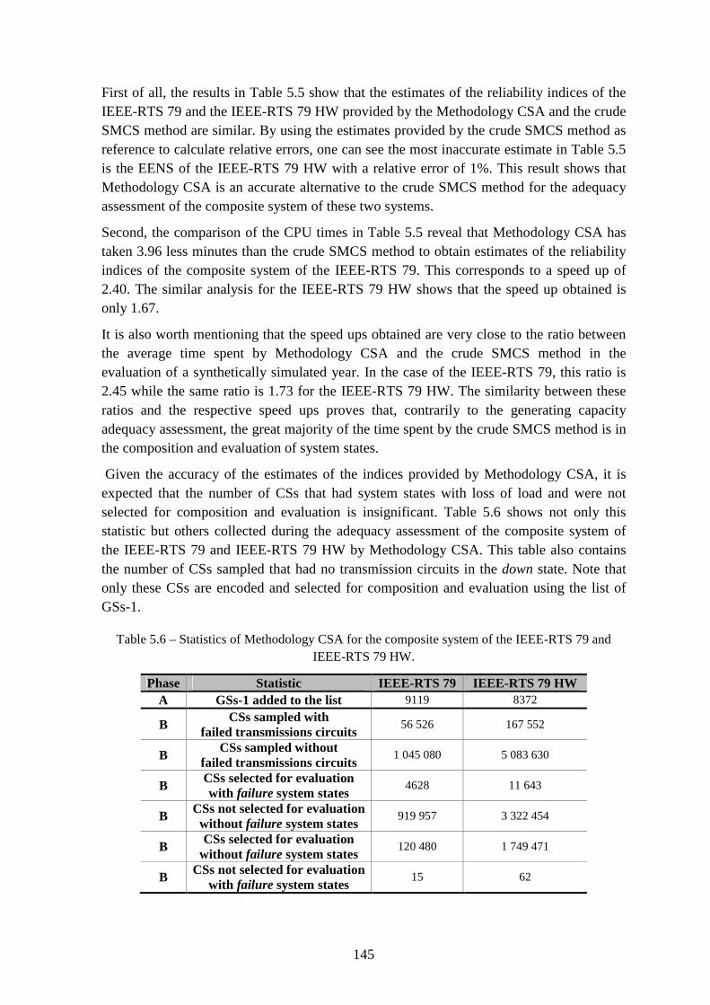
145

First of all, the results in Table 5.5 show that the estimates of the reliability indices of the IEEE-RTS 79 and the IEEE-RTS 79 HW provided by the Methodology CSA and the crude SMCS method are similar. By using the estimates provided by the crude SMCS method as reference to calculate relative errors, one can see the most inaccurate estimate in Table 5.5 is the EENS of the IEEE-RTS 79 HW with a relative error of 1%. This result shows that Methodology CSA is an accurate alternative to the crude SMCS method for the adequacy assessment of the composite system of these two systems.

Second, the comparison of the CPU times in Table 5.5 reveal that Methodology CSA has taken 3.96 less minutes than the crude SMCS method to obtain estimates of the reliability indices of the composite system of the IEEE-RTS 79. This corresponds to a speed up of 2.40. The similar analysis for the IEEE-RTS 79 HW shows that the speed up obtained is only 1.67.

It is also worth mentioning that the speed ups obtained are very close to the ratio between the average time spent by Methodology CSA and the crude SMCS method in the evaluation of a synthetically simulated year. In the case of the IEEE-RTS 79, this ratio is 2.45 while the same ratio is 1.73 for the IEEE-RTS 79 HW. The similarity between these ratios and the respective speed ups proves that, contrarily to the generating capacity adequacy assessment, the great majority of the time spent by the crude SMCS method is in the composition and evaluation of system states.

Given the accuracy of the estimates of the indices provided by Methodology CSA, it is expected that the number of CSs that had system states with loss of load and were not selected for composition and evaluation is insignificant. Table 5.6 shows not only this statistic but others collected during the adequacy assessment of the composite system of the IEEE-RTS 79 and IEEE-RTS 79 HW by Methodology CSA. This table also contains the number of CSs sampled that had no transmission circuits in the down state. Note that only these CSs are encoded and selected for composition and evaluation using the list of GSs-1.

Table 5.6 – Statistics of Methodology CSA for the composite system of the IEEE-RTS 79 and IEEE-RTS 79 HW.

Phase Statistic IEEE-RTS 79 IEEE-RTS 79 HW A GSs-1 added to the list 9119 8372

B CSs sampled with

failed transmissions circuits 56 526 167 552

B CSs sampled without

failed transmissions circuits 1 045 080 5 083 630

B CSs selected for evaluation with failure system states

4628 11 643

B CSs not selected for evaluation without failure system states

919 957 3 322 454

B CSs selected for evaluation without failure system states

120 480 1 749 471

B CSs not selected for evaluation with failure system states

15 62

146

The statistics in Table 5.6 referring to the case of the IEEE-RTS 79 show that only 15 of the 1 045 080 CSs sampled were mistakenly classified as not containing system states with failure. Moreover, 88.5% of the CSs that had no failed transmission circuits were correctly classified. To this total contributes the 0.44% CSs selected for composition and evaluation that had failure system states and the 88.03% CSs not selected for composition and evaluation that contained no loss of load throughout their duration.

Now, consider the statistics in Table 5.6 for the IEEE-RTS 79 HW. The number of CSs incorrectly categorized as not having failure system states is 0.001% of the CSs sampled that had no circuits in the down state. However, the percentage of correctly classified states is only 65.4%, which indicates that a considerable number of CSs were composed and evaluated unnecessarily (more precisely, 34.4% of the CSs sampled). Given the different classification accuracies of Methodology CSA for the IEEE-RTS 79 and IEEE-RTS 79 HW, one can conclude that the classification performance of Methodology CSA is strongly dependent on the characteristics of the system evaluated.

5.8.1.2. Results for the IEEE-MRTS 79

Table 5.7 shows the results of the Methodology CSA and the crude SMCS method for the composite system of the IEEE-MRTS 79. Despite the remarkable speed up of 4.97 of Methodology CSA over the crude SMCS method, the inspection of the estimates of the indices available in this table show important differences.

As a matter of fact, the relative error of the LOLE is 15.6%, 3.6% for the EENS, and 20.8% for the LOLF. Some of these errors are greater than the 5% coefficient of variation used as stopping criterion.

Table 5.7 – Results of Methodology CSA for the composite system of the IEEE-MRTS 79.

IEEE-MRTS 79

Methodology CSA Crude SMCS LOLE (h/yr) 31.011 36.756

EENS (MWh/yr) 5368.87 5567.57 LOLF (occ./yr) 6.095 7.697

Years Simulated 1042 934 System States Composed

and Evaluated 1 093 115 8 639 347

Total CPU Time (min) 22.58 112.20 Phase A CPU Time (min) 0.0115 -

Average CPU Time Required by Phase B to Evaluate a Year (ms)

1296.86 7205.02

The statistics collected for the IEEE-MRTS 79 available Table 5.8 shows that the number of CSs with failure system states that were not selected for composition and evaluation are in line with the inaccurate estimates of the reliability indices provided by Methodology

147

CSA. Accordingly, 0.32% of the 484 380 CSs sampled were incorrectly classified as not having loss of load. This percentage is considerably greater than the equivalent results obtained for composite systems of the IEEE-RTS 79 and IEEE-RTS 79 HW.

Table 5.8 – Statistics of Methodology CSA for the composite system of the IEEE-MRTS 79.

Phase Statistic IEEE-MRTS 79 A GSs-1 added to the list 14 646

B CSs sampled with

failed transmissions circuits 27 139

B CSs sampled without

failed transmissions circuits 484 380

B CSs selected for evaluation with failure system states

4288

B CSs not selected for evaluation without failure system states

423 799

B CSs selected for evaluation without failure system states

54 720

B CSs not selected for evaluation with failure system states

1573

The reason why Methodology CSA cannot provide accurate estimates of the reliability indices for the composite system of the IEEE-MRTS 79 is related to the nature of loss of load events involving transmission circuits. As a matter of fact, some authors have observed that the transmission scenario of the IEEE-MRTS 79 that contributes to the reliability indices the most was no transmission outages [5]. As a matter of fact, this scenario can cause loss of load even if there is sufficient generating capacity to supply the load. Since the EPSO-based PBM did not take capacity limitations of the transmission circuits into account, the information necessary to detect the CSs that have sufficient generating capacity to supply the load but still have loss of load is not passed onto Phase B. For this reason, one can conclude that Methodology CSA cannot be systematically applied to the adequacy assessment of all composite systems. As a matter of fact, Methodology CSA can only be used in systems with specific characteristics, like the IEEE-RTS 79 and the IEEE-RTS 79 HW, where there the transmission network does not have severe capacity limitations.

5.8.2. Methodology CSB

The classification of the CSs sampled in Phase B can be done by analyzing its GS and TS separately. Accordingly, two lists must be used: one containing GSs-1 and other including TSs. The list of GSs-1 is created by using the EPSO-based PBM. This search process is named Phase A1.

Likewise, the EPSO-based PBM can be used to build the list of TSs. This second search process, which is called Phase A2, assumes that the state of the generating units is fixed. Phase A1 is used to define the state of the generating units in Phase A2. The selection of

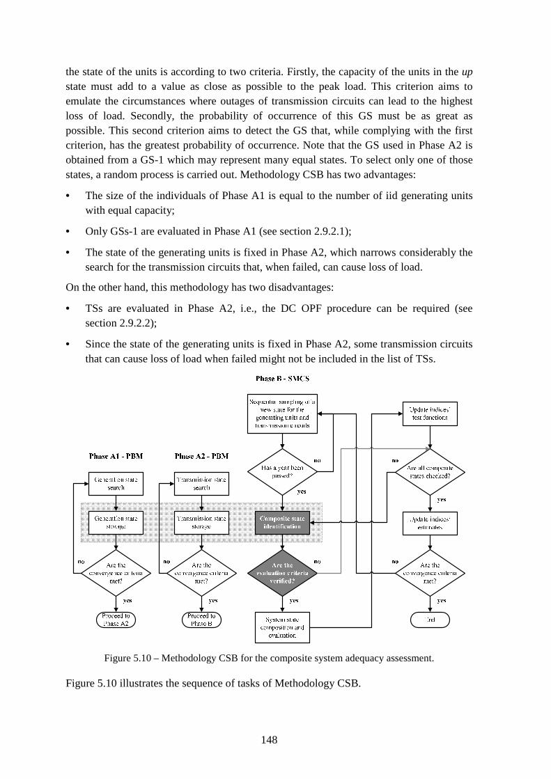
148

the state of the units is according to two criteria. Firstly, the capacity of the units in the up state must add to a value as close as possible to the peak load. This criterion aims to emulate the circumstances where outages of transmission circuits can lead to the highest loss of load. Secondly, the probability of occurrence of this GS must be as great as possible. This second criterion aims to detect the GS that, while complying with the first criterion, has the greatest probability of occurrence. Note that the GS used in Phase A2 is obtained from a GS-1 which may represent many equal states. To select only one of those states, a random process is carried out. Methodology CSB has two advantages:

• The size of the individuals of Phase A1 is equal to the number of iid generating units with equal capacity;

• Only GSs-1 are evaluated in Phase A1 (see section 2.9.2.1);

• The state of the generating units is fixed in Phase A2, which narrows considerably the search for the transmission circuits that, when failed, can cause loss of load.

On the other hand, this methodology has two disadvantages:

• TSs are evaluated in Phase A2, i.e., the DC OPF procedure can be required (see section 2.9.2.2);

• Since the state of the generating units is fixed in Phase A2, some transmission circuits that can cause loss of load when failed might not be included in the list of TSs.

Figure 5.10 – Methodology CSB for the composite system adequacy assessment.

Figure 5.10 illustrates the sequence of tasks of Methodology CSB.

149

Three criteria are used to detect the CSs sampled in Phase B that needed composition and evaluation. If the string created for the TS is in the list of the TSs or if the last system state evaluated has loss of load, then the CS proceeds to composition and evaluation. If not, a string is created for the GS-1 of the CS. If this second string is one of the keys of the hash table of GSs-1, the CS under analysis is composed and evaluated. If not, it is considered that no loss of load occurs throughout the duration of the CS. Only Strategy C is used to represent the time-dependent capacity of the generating units in Phase A1 and Phase A2 (see section 5.7.1).

Similarly to Methodology CSA, Methodology CSB was used to obtain estimates of the reliability indices of the composite system of the IEEE-RTS 79, the IEEE-RTS 79 HW and the IEEE-MRTS 79. All estimates of the annual reliability indices obtained have a coefficient of variation less than or equal to 5%. Once again, the simulations were conducted on an Intel Core i7-2600 CPU (3.40 GHz). Methodology CSB and the crude SMCS were implemented in JAVA language.

The parameters of the Phase A1 used are the following:

• Number of individuals: n = 20;

• Number of replications per individual: m = 2;

• Mutation rate: τ = 0.4;

• Communication probability: P = 0.6;

• Probability threshold: pmin = 1×10-15;

• Annualized reliability index selected to gauge the convergence: EPNS;

• Tolerance for the improvement of the annualized EPNS: ε = 0.01;

• Maximum number of generations without significant improvement on the estimate of the annualized EPNS: NMAX = 50.

Conversely, the parameters of the Phase A2 are:

• Number of individuals: n = 40;

• Number of replications per individual: m = 2;

• Mutation rate: τ = 0.4;

• Communication probability: P = 0.6;

• Probability threshold: pmin = 1×10-10;

• Annualized reliability index selected to gauge the convergence: EPNS;

• Tolerance for the improvement of the annualized EPNS: ε = 0.01;

• Maximum number of generations without significant improvement on the estimate of the annualized EPNS: NMAX = 50.

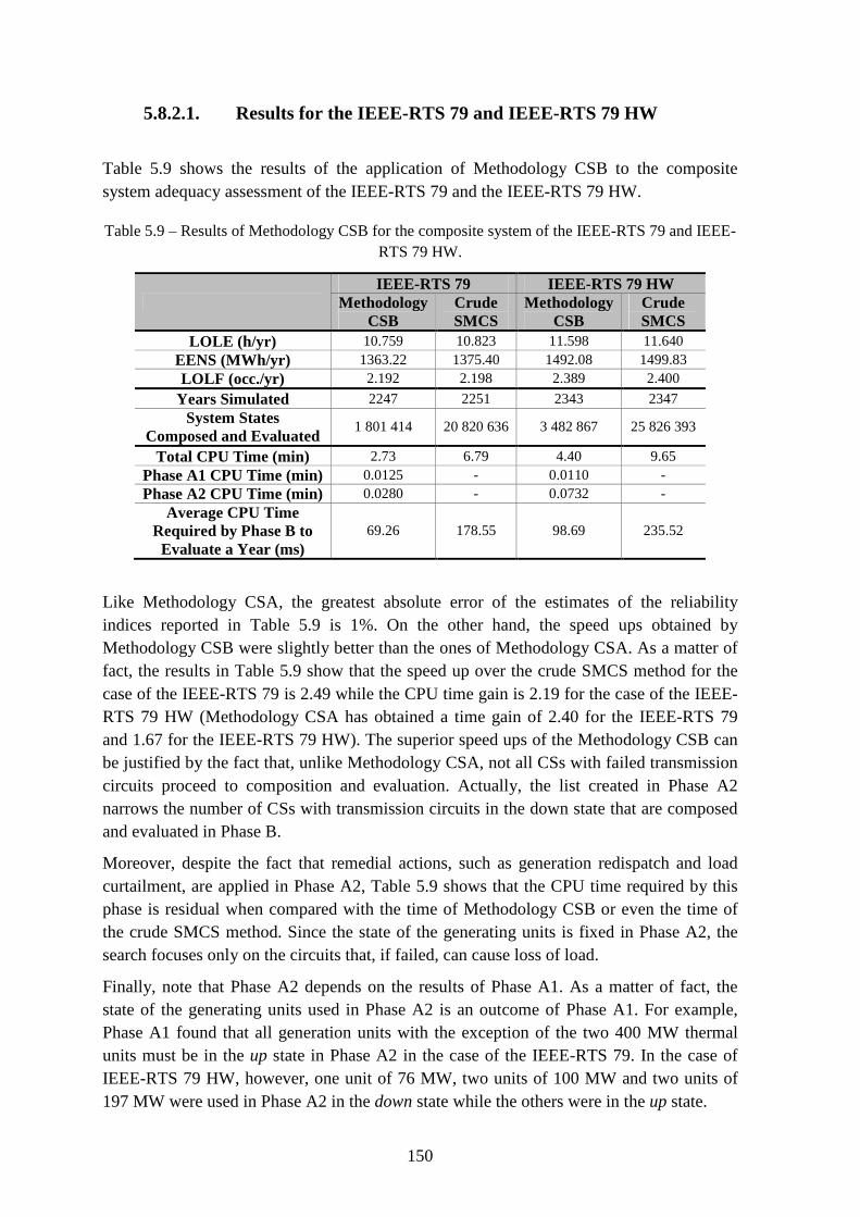
150

5.8.2.1. Results for the IEEE-RTS 79 and IEEE-RTS 79 HW

Table 5.9 shows the results of the application of Methodology CSB to the composite system adequacy assessment of the IEEE-RTS 79 and the IEEE-RTS 79 HW.

Table 5.9 – Results of Methodology CSB for the composite system of the IEEE-RTS 79 and IEEE-RTS 79 HW.

IEEE-RTS 79 IEEE-RTS 79 HW

Methodology CSB

Crude SMCS

Methodology CSB

Crude SMCS

LOLE (h/yr) 10.759 10.823 11.598 11.640 EENS (MWh/yr) 1363.22 1375.40 1492.08 1499.83 LOLF (occ./yr) 2.192 2.198 2.389 2.400

Years Simulated 2247 2251 2343 2347 System States

Composed and Evaluated 1 801 414 20 820 636 3 482 867 25 826 393

Total CPU Time (min) 2.73 6.79 4.40 9.65 Phase A1 CPU Time (min) 0.0125 - 0.0110 - Phase A2 CPU Time (min) 0.0280 - 0.0732 -

Average CPU Time Required by Phase B to Evaluate a Year (ms)

69.26 178.55 98.69 235.52

Like Methodology CSA, the greatest absolute error of the estimates of the reliability indices reported in Table 5.9 is 1%. On the other hand, the speed ups obtained by Methodology CSB were slightly better than the ones of Methodology CSA. As a matter of fact, the results in Table 5.9 show that the speed up over the crude SMCS method for the case of the IEEE-RTS 79 is 2.49 while the CPU time gain is 2.19 for the case of the IEEE-RTS 79 HW (Methodology CSA has obtained a time gain of 2.40 for the IEEE-RTS 79 and 1.67 for the IEEE-RTS 79 HW). The superior speed ups of the Methodology CSB can be justified by the fact that, unlike Methodology CSA, not all CSs with failed transmission circuits proceed to composition and evaluation. Actually, the list created in Phase A2 narrows the number of CSs with transmission circuits in the down state that are composed and evaluated in Phase B.

Moreover, despite the fact that remedial actions, such as generation redispatch and load curtailment, are applied in Phase A2, Table 5.9 shows that the CPU time required by this phase is residual when compared with the time of Methodology CSB or even the time of the crude SMCS method. Since the state of the generating units is fixed in Phase A2, the search focuses only on the circuits that, if failed, can cause loss of load.

Finally, note that Phase A2 depends on the results of Phase A1. As a matter of fact, the state of the generating units used in Phase A2 is an outcome of Phase A1. For example, Phase A1 found that all generation units with the exception of the two 400 MW thermal units must be in the up state in Phase A2 in the case of the IEEE-RTS 79. In the case of IEEE-RTS 79 HW, however, one unit of 76 MW, two units of 100 MW and two units of 197 MW were used in Phase A2 in the down state while the others were in the up state.

151

Table 5.10 contains the statistics of Methodology CSB for the composite system of the IEEE-RTS 79 and IEEE-RTS 79 HW. In addition to the usual statistics of the classification process made in Phase B, this table contains the number of GSs-1 and the TSs added to their respective lists.

Table 5.10 – Statistics of Methodology CSB for the composite system of the IEEE-RTS 79 and IEEE-RTS 79HW.

Phase Statistic IEEE-RTS 79 IEEE-RTS 79 HW A1 GSs-1 added to the list 9119 7932 A2 TSs added to the list 329 1267

B CSs sampled 1 102 090 5 260 106

B CSs selected for evaluation with failure system states

4818 12 016

B CSs not selected for evaluation without failure system states

970 191 4 505 445

B CSs selected for evaluation

without failure system states 127 063 742 590

B CSs not selected for evaluation

with failure system states 18 55

The analysis of the results in Table 5.10 for the IEEE-RTS 79 reveals that 88.47% of the CSs sampled in Phase B were correctly identified. Therefore, the accuracy of the classification process of Methodology CSB is similar to the accuracy of Methodology CSA for the composite system of the IEEE-RTS 79. On the other hand, the percentage of incorrectly categorized CSs for the IEEE-RTS 79 HW is 14.12%. The same percentage of CSs incorrectly categorized by Methodology CSA for the IEEE-RTS 79 HW is 34.4%. Hence, the use Methodology CSB permits increasing not only the speed ups but also the accuracy of the classification process for composite systems with renewable energy resources like the IEEE-RTS 79 HW.

5.8.2.2. Results for the IEEE-MRTS 79

Table 5.11 and Table 5.12 contain, respectively, the results and the statistics of Methodology CSB for the composite system adequacy assessment of the IEEE-MRTS 79. Like Methodology CSA, these tables show that the estimates provided by the Methodology CSB for the indices of the composite system of the IEEE-MRTS 79 have significant errors. As a matter of fact, the relative error of the LOLE is 15.8%, 5.4% for the EENS, and 20.7% for the LOLF. Yet, the speed up obtained was 5.24, which is slightly better than the time gain of Methodology CSA over the crude SMCS method.

From the results reported in the last two tables, one can conclude that the accuracy problem of Methodology CSA has not been circumvented by Methodology CSB. As a matter of fact, Methodology CSB is not able to identify the CSs that have loss of load despite having sufficient generating capacity to supply the load.

152

Table 5.11 – Results of Methodology CSB for the composite system of the IEEE-MRTS 79.

IEEE-MRTS 79

Methodology CSB Crude SMCS LOLE (h/yr) 30.948 36.756

EENS (MWh/yr) 5266.45 5567.57 LOLF (occ./yr) 6.104 7.697

Years Simulated 984 934 System States

Composed and Evaluated 1 044 509 8 639 347

Total CPU Time (min) 21.41 112.20 Phase A1 CPU Time (min) 0.0122 - Phase A2 CPU Time (min) 0.0694 -

Average CPU Time Required by Phase B to Evaluate a Year (ms)

1297.78 7205.02

Table 5.12 – Statistics of Methodology CSB for the composite system of the IEEE-MRTS 79.

Phase Statistic IEEE-MRTS 79 A1 GSs-1 added to the list 9119 A2 TSs added to the list 1486

B CSs sampled 483 097

B CSs selected for evaluation with failure system states

5902

B CSs not selected for evaluation without failure system states

399 702

B CSs selected for evaluation

without failure system states 75 989

B CSs not selected for evaluation

with failure system states 1504

Since the two methodologies have the same accuracy issue and similar speed ups, one can assume that Methodology CSA and Methodology CSB are equivalent. However, given that Methodology CSB has a better time-efficiency, one can conclude that this methodology is superior to Methodology CSA.

5.8.3. Methodology CSC

The basic idea of Methodology CSC is to search for and collect CSs in Phase A and use the resulting list to classify the CSs sampled in Phase B. Thus, the individuals of the EPSO-based PBM have a size equal to the size of GSs-2 plus the size of TSs. The representation of CSs in the EPSO-based PBM is according to section 5.6.1.

The main advantage of Methodology CSC is:

• Phase A is carried out in the space of CSs.

Conversely, its main disadvantage is:

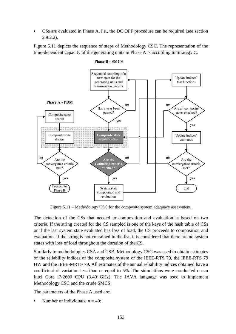
153

• CSs are evaluated in Phase A, i.e., the DC OPF procedure can be required (see section 2.9.2.2).

Figure 5.11 depicts the sequence of steps of Methodology CSC. The representation of the time-dependent capacity of the generating units in Phase A is according to Strategy C.

Figure 5.11 – Methodology CSC for the composite system adequacy assessment.

The detection of the CSs that needed to composition and evaluation is based on two criteria. If the string created for the CS sampled is one of the keys of the hash table of CSs or if the last system state evaluated has loss of load, the CS proceeds to composition and evaluation. If the string is not contained in the list, it is considered that there are no system states with loss of load throughout the duration of the CS.

Similarly to methodologies CSA and CSB, Methodology CSC was used to obtain estimates of the reliability indices of the composite system of the IEEE-RTS 79, the IEEE-RTS 79 HW and the IEEE-MRTS 79. All estimates of the annual reliability indices obtained have a coefficient of variation less than or equal to 5%. The simulations were conducted on an Intel Core i7-2600 CPU (3.40 GHz). The JAVA language was used to implement Methodology CSC and the crude SMCS.

The parameters of the Phase A used are:

• Number of individuals: n = 40;

Composite state

search

Composite state

storage

Are the

convergence criteria

met?

Phase A - PBM

yes

no

Proceed to

Phase B

Sequential sampling of a

new state for the

generating units and

transmission circuits

Composite state

identification

Are the

evaluation criteria

verified?

Has a year been

passed?

System state

composition and

evaluation

Update indices’

test functions

Are all composite

states checked?

Update indices’

estimates

Are the

convergence criteria

met?

End

yes

yes

no

no no

yes

yes

no

Phase B - SMCS

154

• Number of replications per individual: m = 2;

• Mutation rate: τ = 0.4;

• Communication probability: P = 0.6;

• Probability threshold: pmin = 1×10-15;

• Annualized reliability index selected to gauge the convergence: EPNS;

• Tolerance for the improvement of the annualized EPNS: ε = 0.01;

• Maximum number of generations without significant improvement on the estimate of the annualized EPNS: NMAX = 50.

5.8.3.1. Results for the IEEE-RTS 79 and IEEE-RTS 79 HW

Table 5.13 shows the results of Methodology CSC for composite system adequacy assessment of the IEEE-RTS 79 and the IEEE-RTS 79 HW. This table contains the estimates of the LOLE, EENS and LOLF provided by Methodology CSC and the crude SMCS method for the two test systems.

Table 5.13 – Results of Methodology CSC for the composite system of the IEEE-RTS 79 and IEEE-RTS 79 HW.

IEEE-RTS 79 IEEE-RTS 79 HW

Methodology CSC

Crude SMCS

Methodology CSC

Crude SMCS

LOLE (h/yr) 10.518 10.823 10.920 11.640 EENS (MWh/yr) 1333.29 1375.40 1380.71 1499.83 LOLF (occ./yr) 2.145 2.198 2.266 2.400

Years Simulated 2258 2251 2370 2347 System States

Composed and Evaluated 1 781 436 20 820 636 8 665 976 25 826 393

Total CPU Time (min) 3.02 6.79 5.87 9.65 Phase A CPU Time (min) 0.613 - 0.459 -

Average CPU Time Required by Phase B to Evaluate a Year (ms)

60.91 178.55 123.18 235.52

To begin with, the relative error of the LOLE of the IEEE-RTS 79 is 2.8% whereas the error of the EENS is 3.1%, and the error of the LOLF is 2.4%. The same analysis for the case of the IEEE-RTS 79 HW reveals that the error is 6.2% for the case of the LOLE, 7.9% for the EENS and 5.6% for LOLF. By comparing these errors with the ones obtained by the other two methodologies for these two test systems, one can conclude that Methodology CSC has the worst accuracy. Nevertheless, the estimates provided by Methodology CSC are well within the accurate 95% interval of confidence of these indices. Despite having the poorest accuracy of all methodologies, Methodology CSC can

155

provide estimates of the indices of the composite system of the IEEE-RTS 79 and the IEEE-RTS 79 HW with tolerable errors.

Secondly, consider the CPU time in Table 5.13 required by Methodology CSC and the crude SMCS method to provide estimates of the annual reliability indices. From these times, one can see that the speed up of Methodology CSC over the crude SMCS method is 2.24 for the IEEE-RTS 79 and 1.64 for the IEEE-RTS 79 HW. Hence, Methodology CSC is the one with the lowest speed ups between the three methodologies.

The poorest efficiency of Methodology CSC is caused in part by the greater CPU time required by Phase A. As a matter of fact, the time required by Phase A of Methodology CSC is 53.3 times more than the time of Phase A of Methodology CSA and 15.14 times more than the combined CPU time of Phase A1 and Phase A2 of Methodology CSB. On the other hand, the average time required by Phase B to evaluate a year of the IEEE-RTS 79 is 60.91 ms in the case of Methodology CSC, 69.26 ms for Methodology CSB and 72.78 ms in the case of Methodology CSA. This shows that the time lost by Methodology CSC in Phase A is recovered in Phase B.

The use of the EPSO-based PBM to search in the space of CSs must be done with caution. A way to avoid spending too much time in Phase A is to use information from the evaluation of CSs to create new individuals. For instance, if a given CS has a considerable number of transmission circuits operating close to their limits, one can remove one of these circuits at a time to find if the resulting CSs meet the requirements to enter the list of states.

Consider now Table 5.14. This table has the statistics of Methodology CSC for the composite system of the IEEE-RTS 79 and IEEE-RTS 79 HW.

Table 5.14 – Statistics of Methodology CSC for the composite system of the IEEE-RTS 79 and IEEE-RTS 79 HW.

Phase Statistic IEEE-RTS 79 IEEE-RTS 79 HW A CSs added to the list 49 665 39 457

B CSs sampled 1 107 394 5 320 878

B CSs selected for evaluation with failure system states

4703 11 414

B CSs not selected for evaluation without failure system states

978 640 3 506 658

B CSs selected for evaluation

without failure system states 123 894 1 802 050

B CSs not selected for evaluation

with failure system states 157 756

The results in Table 5.14 show that the number of CSs not selected for composition and evaluation with failure system states is almost 10 times greater than the equivalent statistic obtained for methodologies CSA and CSB. Luckily, the misclassification of these CSs did not affect considerably the estimates of the indices.

156

Consider also the number of CSs in the respective lists. Accordingly, the size of the lists created in Phase A of Methodology CSC for the IEEE-RTS 79 and IEEE-RTS 79 HW is considerably greater than the size of the lists of GSs-1 and TSs of the other two methodologies. Even so, the average time required by Phase A to evaluate one year is similar to the time reported by the other methodologies. Given the fact that the three methodologies have sampled, composed, and evaluated an equivalent number of CSs in Phase B (see Table 5.6, Table 5.10, and Table 5.14), one can conclude the performance of the hash table that implement the concept of list of states is not considerably affected by the number of states contained by it.

5.8.3.2. Results for the IEEE-MRTS 79

Table 5.15 shows the results of Methodology CSC for the composite system adequacy assessment of the IEEE-MRTS 79.

Table 5.15 – Results of Methodology CSC for the composite system of the IEEE-MRTS 79.

IEEE-MRTS 79

Methodology CSC Crude SMCS LOLE (h/yr) 35.441 36.756

EENS (MWh/yr) 5331.34 5567.57 LOLF (occ./yr) 7.467 7.697

Years Simulated 936 934 System States

Composed and Evaluated 2 873 954 8 639 347

Total CPU Time (min) 53.45 112.20 Phase A CPU Time (min) 5.00 -

Average CPU Time Required by Phase B to Evaluate a Year (ms)

3102.26 7205.02

The results in Table 5.15 show that the relative error of the estimates provided by Methodology CSC for the IEEE-MRTS 79 is 3.6% for the LOLE, 4.2% for the EENS, and 3.0% for the LOLF. The comparison of these errors with the ones obtained by the other methodologies demonstrates that only Methodology CSC can accurately replace the crude SMCS method in the estimation of reliability indices of the composite system of the IEEE-MRTS 79.

As a matter of fact, the EPSO-based PBM is able to capture the CSs that have sufficient generating capacity to supply the peak load and still have loss of load. Clearly, Methodology CSC can be used to evaluate all systems.

Unfortunately, the speed up obtained of Methodology CSC over the crude SMCS method is only 2.1. Part of this poor speed up is due to the 5 minutes required by Phase A. This result proves that searching in the space of CSs is time-consuming.

157

Table 5.16 presents the statistics of Methodology CSC collected during the composite system adequacy assessment of the IEEE-MRTS 79. As expected, the number of CSs that had system states with loss of load and were not selected for composition and evaluation is small but not negligible (0.07% of the total number of CSs sampled).

Note that, in the case of the IEEE-MRTS 79, this type of incorrect classified CSs is less frequent in Methodology CSC than in the other two methodologies. This statistic proves why Methodology CSC is able to provide accurate estimates of the reliability indices of the composite system of the IEEE-MRTS 79.

Table 5.16 – Statistics of Methodology CSC for the composite system of the IEEE-MRTS 79.

Phase Statistic IEEE-MRTS 79 A CSs added to the list 73 312

B CSs sampled 459 395

B CSs selected for evaluation with failure system states

6726

B CSs not selected for evaluation without failure system states

261 019

B CSs selected for evaluation without failure system states

191 319

B CSs not selected for evaluation

with failure system states 331

Finally, note that the classification accuracy of Methodology CSC is only 58.8%. This means that a considerable number of CSs are composed and evaluated only to find that they do not have system states with loss of load. If the number of CSs incorrectly selected for classification and evaluation can be reduced, the speed up of Methodology CSC would be increased.

5.9. Conclusions

This chapter showed how PBMs can be used to improve the efficiency of the sequential MCS method. Since real power systems are traditionally reliable, the majority of the system states do not have loss of load. Hence, the methodology proposed in this chapter relies on a list of states that PBMs make available at the end of the search process to help detect the states sampled by sequential MCS method that need composition and evaluation.

Basically, the methodology proposed consists of two phases. The first phase, which has been named Phase A, is aimed to create a list of states that cannot supply the peak load. A PBM based on the EPSO metaheuristic is used to perform this task, taking advantage of its superior capabilities of this metaheuristic to make a broad coverage of the state space. This list is subsequently used in Phase B, whose core is the sequential MCS method, to enhance the time-efficiency of the composition and evaluation of system states.

This chapter started with an overview of the techniques reported in the literature to speed up the composition and evaluation stages of MCS method. Next, a brief introduction to

158

metaheuristic optimization was carried out to lay down the foundation for the subsequent description of the EPSO metaheuristic for single objective optimization.

After that, PBMs were formally examined. These methods can compute estimates of the reliability indices based on an intelligent enumeration process. Due to the inherent characteristics of PBMs, they always underestimate the correct value of the indices. In addition, these methods do not guarantee that the estimates provided are accuracy. Fortunately, PBMs offer a list with the states that most contribute to the annualized reliability indices as a byproduct. This is list can be used by the sequential MCS method as classifier for the states sampled.

To help understand the methodology proposed, the concepts of generation, transmission and composite states were introduced. Accordingly, a GS includes the state of the generating units. A TS includes the state of the transmission circuits. Finally, a CS includes the state of the generation and transmission circuits, i.e. it contains a GS and a TS. Each of these states has a unique code. This code is included in a fast access database, which implements computationally the concept of lists of states.

The methodology proposed was applied to the generating capacity adequacy assessment of three power systems that include wind and hydro intermittency: the IEEE-RTS 79, the IEEE-RTS 96 and the IEEE-RTS 96 HW. The results of these experiments showed noteworthy gains in the time-efficiency of the sequential MCS method. These gains range between 2.44 to 4.85. In spite of being incomparable with the gains obtained in the previous chapter, the methodology proposed is able to provide accurate probability distributions for the reliability indices.

The experiments carried out also showed that the best strategy to model the capacity of the hydro units and WTGs in Phase A is Strategy D. As a matter of fact, the underestimation of the capacity of these units makes possible the fastest savings in net CPU time while providing estimates of the reliability indices with the lowest errors.

It was also observed that the accuracy of the classification process cannot be easily controlled and depends on the characteristics of the system being evaluated. As a general but no universal observation, the number of system states that have no loss of load but still have to be composed an evaluated should increase in order to obtain accurate estimates of the reliability indices.

The methodology proposed was also applied to the composite system adequacy assessment of three power systems that include wind and hydro intermittency: the IEEE-RTS 79, the IEEE-RTS 79 HW and the IEEE-MRTS 79. More specifically, three methodologies were proposed taking advantage of the fact that a CS is composed by a GS and a TS.

The first methodology, which was named Methodology CSA, obtained a speed up of 2.4 for the IEEE-RTS 79, a speed up of 1.67 for the IEEE-RTS 79 HW and a speed up of 4.97 for the IEEE-MRTS 79. Only in the case of the IEEE-MRTS 79 were obtained inaccurate estimates of the reliability indices. For this reason, Methodology CSA can only be applied in systems where the loss of load events involving the transmission network can only be caused by outages of circuits.

159

The second methodology, which was termed Methodology CSB, attained a speed up of 2.49 for the IEEE-RTS 79, a speed up of 2.19 for the IEEE-RTS 79 HW and a speed up of 5.24 for the IEEE-MRTS 79. Like Methodology CSB, the estimates of the reliability indices for the IEEE-MRTS 79 are affected by considerable errors. Bearing in mind that better speed ups were obtained and that the cause for the inaccuracies observed for the composite system of the IEEE-MRTS 79 is alike, it can be concluded that Methodology CSB is better than Methodology CSA.

Methodology CSC, which, unlike the other two methodologies, searches for CSs in Phase A, has got a speed up of 2.24 for the IEEE-RTS 79, a speed up of 1.64 for the IEEE-RTS 79 HW and a speed up of 2.1 for the IEEE-MRTS 79. Note that this methodology is the only one that can provide accurate estimates of the reliability indices for the composite systems considered. However, since the EPSO-based PBM makes the search in the space of CSs, this methodology has the Phase A that takes the most time.

Given the different efficiency and accuracy of the three methodologies, one can conclude that methodologies CSB and CSC can be used alternatively to evaluate the adequacy of the composite systems that best fit their characteristics.

160

161

Chapter 6

General Conclusions

6.1. Overall Conclusions

It is undeniable that the transition to sustainable power systems will create new and complex problems that need appropriate modeling. The long-term adequacy assessment of the generating capacity and composite system are strong examples of such problems. As a matter of fact, the replacement of thermal generating units by intermittent generation can have an important impact on the adequacy of supply. Hence, the appropriate modeling of this type of generation facilities is imperative so that the impacts that the intermittent power can have on the continuity of supply are able to be assessed as accurately as possible.

Clearly, one of the most suitable tools to assess the adequacy of power systems with renewable resources is the sequential MCS method. By synthetically generating operating/repairing times for the components of the system, this method is able to inherently incorporate the fluctuating capacity of renewable power sources. However, the modeling flexibility of the sequential MCS method is offset by an important drawback: the time-consuming sequential sampling mechanism.

As a matter of fact, simulation methods, like the sequential MCS method, estimate reliability indices by counting and analyzing successive samples of system states. These samples are drawn according to the stochastic behavior of the system. In systems where the occurrence of the states that contribute to the indices is rare, the accurate prediction of the behavior of the system as a whole might require a considerable number of samplings and, consequently, a large number of state evaluations. Moreover, most of the evaluations carried out detect that the most of the states sampled do not have loss of load, i.e., they are applied to just to identify a small set of states that contribute directly to the reliability indices, i.e., the failure ones.

Accordingly, the aim of this dissertation is to analyze and propose methodologies that can improve the time-efficiency the sequential MCS method while retaining all its modeling flexibility and unique results. For this purpose, two approaches can be used: the improvement of the sampling efficiency and the improvement of the state evaluation efficiency. From these approaches, two hypotheses were proposed in the first chapter of this dissertation.

162

The second chapter of this dissertation started with a general introduction on power systems adequacy assessment. This introduction emphasized the unique features of the sequential MCS method by distinguishing it from other methods that can be used for the adequacy assessment of power systems. In addition, the sequential MCS method implemented in the scope of this dissertation was presented in this chapter. Several experiments were carried out to assess the accuracy of the sequential MCS method implemented. The reliability indices estimated in these experiments were compared with the ones published in the literature. From the comparisons, it was concluded that the sequential MCS method developed can provide accurate estimates of the reliability indices not only for the generating capacity but also for the composite system of variants of the IEEE-RTS 79 and the IEEE-RTS 96 that have hydro units and WFs.

Given the ability of the sequential MCS method to include accurate models for wind intermittency, a simple methodology was proposed to detect, in a planning perspective, whether wind curtailment events are due to the enforcement of operating strategies and/or load deficit, the failure and/or capacity limits of transmission circuits or the simultaneous occurrence of both these events. Accordingly, the following categorization for these events was proposed:

• Event A: wind power curtailment due to the enforcement of the inertial constraint and/or load deficit;

• Event B: wind power curtailment due to transmission circuit failures and/or capacity limits;

• Event C: wind power curtailment due to the simultaneous occurrence of events A and B.

The inertial constraint is a simple model that accounts for the dispatching preferences of system operators when a great share of the generating capacity is intermittent. In simple terms, this model assumes that a fixed amount of load must always be supplied by a given set of generating units regardless of the hourly load variation.

The different wind power curtailment events under a strategy of maximum use of wind power were analyzed. It was shown that, for the cases studied, the transmission network does not limit the use of wind power as severely as the inertial constraint. In addition, the transmission circuit that limits the use of wind power the most depends on the loading status of the transmission network. Note that this methodology can detect this circuit automatically.

The analysis of the wind power curtailment events also evidenced that a growing inertial load involves considerable amounts of wind energy not used. Moreover, the experiments proved that considerable wind power is curtailed even if the inertial load remains constant. This corresponds to the scenario where the system load is insufficient to accommodate the additional wind capacity.

The impact of the wind and thermal technologies on the adequacy of the composite system was also investigated. On one hand, the experiments carried out proved that if the EAME is used as performance measure instead of the installed capacity, WFs can provide lower

163

LOLE and EENS than a thermal unit. On the other hand, it was verified that the same conclusions are not valid for the case of the LOLF. Hence, the comparison of these two technologies in terms of the adequacy of supply strongly depends on the performance measure and the reliability indice selected.

The fourth chapter of this dissertation investigated Hypothesis 1, which is:

• Hypothesis 1: the CE method can make the sequential MCS method applied to power systems more efficient by sampling and evaluating only the states that are most important to the estimators of the reliability indices.

For that purpose, this chapter included a brief introduction to the CE method for rare-event simulation. After that, the equations of the standard CE optimization algorithm for the generating capacity adequacy assessment (PC1) were analyzed. This analysis demonstrated that the optimal IS distribution can be calculated instead of estimated by simply dividing the annualized indices of different system configurations. Consequently, a new CE-based algorithm (PC2) for the generating capacity was proposed. The examination of PC2 has proven that this new CE-based algorithm can calculate distortions similar to the ones estimated by PC1 without requiring extra CPU time. Clearly, the straightforwardness of PC2 is its main advantage.

Chapter 4 also proposed a CE optimization algorithm for the composite system adequacy assessment (PC3). The distorted unavailability of the generating units provided by PC3 were compared with the ones provided by PC2 (note that PC2 can only calculate distortions for the generating units). This comparison demonstrated that, for the three variants of the IEEE-RTS 79 evaluated, the distortions provided by PC2 are not very different from the ones estimated by PC3. Moreover, the distorted parameters of the transmission circuits provided by PC3 have not presented significant differences from their original unavailability. Bearing this in mind and knowing that PC2 is considerably faster than PC3, an investigation of the CPU time required by the two CE-based algorithms and the CE/IS sequential MCS was carried out. This analysis showed that the time lost by PC3 is easily recovered in the subsequent CE/IS sequential MCS method. Without doubt, PC3 is the best choice for accelerating the composite system adequacy assessment via the sequential MCS method. Nonetheless, PC2, which provides similar speed ups to PC3, can still be a competitive alternative if one takes into account that the implementation of PC2 is much simpler than the one of PC3.

Four strategies to model the generating units with time-dependent capacity in PC1, PC2 and PC3 have also been proposed in this fourth chapter:

• Strategy A – random sampling of realizations of the generating capacities from the annual series;

• Strategy B – computation of the average capacity from the annual series and use it as the capacity that the unit provides in the up state;

• Strategy C – selection of the maximum capacity from the annual series and use it as the capacity that the unit provides in the up state;

164

• Strategy D – selection of the minimum capacity from the annual series and use it as the capacity that the unit provides in the up state.

Strategies B, C and D assume that WTGs do not undergo forced outages. Strategy A can only be used in the case of PC1 and PC3 whereas strategies B, C and D can be applied in PC1, PC2 and PC3. The analysis of the CPU times required by the CE/IS sequential MCS method for the adequacy assessment of the generating capacity and composite system of the IEEE-RTS 79 HW, revealed that Strategy C is the one that leads to the greatest speed ups. Moreover, strategies A and B provide not only similar distorted unavailability for the system components but also comparable speed ups, which indicate that they are equivalent. Finally, the lowest time gains are obtained when Strategy D is used.

Table 6.1 reviews the speed ups obtained by the CE/IS sequential MCS method over the crude sequential MCS method for the adequacy assessment of the generating capacity of the IEEE-RTS 79 and the composite system of the IEEE-RTS 79 and IEEE-MRTS 79.

Table 6.1 – Summary of the speed ups of the sequential MCS method according to Hypothesis 1.

System Generating Capacity Composite System

Speed up Speed up IEEE-RTS 79 62.5 86.3

IEEE-MRTS 79 - 3.36

The drawback of using the CE/IS sequential MCS method is that the information necessary to obtain the probability distributions of the reliability indices is lost.

The second hypothesis of this dissertation for improving the efficiency of the sequential MCS method consists of:

• Hypothesis 2: The list of states created by PBMs can be used as a fast and accurate selector and pre-classifier for the interesting states to be sampled by the sequential MCS method.

Differently from the CE/IS sequential MCS method, the gain in CPU time result from avoiding the composition and evaluation of system states that do not have loss of load. The pre-selection of system states can be done by using automatic classifiers, such as ANN. However, the classification process explored relies on the list of states provided by PBMs.

The methodology proposed to explore Hypothesis 2 consists of two phases. The first phase, which was named Phase A, constructs a list of states that cannot supply the peak load. This task is performed by a PBM based on the EPSO metaheuristic. The list of states is subsequently used in Phase B, whose core is the sequential MCS method, to decide if the sampled states should move on to composition and evaluation.

The core of the methodology proposed is the concepts of generation, transmission and composite states. These are the states searched by the EPSO-based PBM. They are only saved in the list if they cannot supply the peak load and if their probability is greater than or equal to a given threshold. Subsequently, the sequential MCS method is used to sample generation, transmission or composite states and their respective duration. If they are in the

165

list, the load and other time-dependent characteristics are sequentially followed to form system states that are evaluated subsequently. If there are not, it is assumed that no loss of load occurs throughout its duration. Obviously, the net gains depends on the time spent creating the list and on the time saved by using the methodology proposed instead of following the traditional state evaluation procedure of the sequential MCS method.

Since the EPSO-based PBM is based on the state-space representation, strategies B, C and D proposed in Chapter 4 to model the generating units with time-dependent capacity can be also used in Phase A of the proposed methodology. The experiments carried out showed that Strategy D allows the greatest savings in CPU time while providing estimates of the reliability indices with the lowest errors.

The methodology proposed was applied to the generating capacity adequacy assessment of three power systems that include wind and hydro intermittency: the IEEE-RTS 79, the IEEE-RTS 96 and the IEEE-RTS 96 HW. The experiments revealed significant gains in CPU time without compromising the accuracy of the estimates of the reliability indices. Moreover, it was observed that the accuracy of the classification process is not easily controlled and depends on the characteristics of the system being evaluated. As a general observation, the number of system states that have no loss of load but still are composed an evaluated must increase in order to obtain estimates of the indices with better accuracy.

The methodology proposed was also applied to the composite system adequacy assessment of three power systems that include wind and hydro intermittency: the IEEE-RTS 79, the IEEE-RTS 79 HW and the IEEE-MRTS 79. More specifically, three methodologies were proposed: Methodology CSA, Methodology CSB and Methodology CSC. The results showed that only Methodology CSC is able to provide accurate estimates of the reliability indices for all composite systems. Alternatively, the speed up of Methodology CSB outperforms that of Methodology CSC when the transmission system does not cause loss of load when there is enough generating capacity to supply the load. To sum up, methodologies CSB and CSC can be used to evaluate the adequacy of the systems that best fit their characteristics.

Table 6.2 – Summary of the speed ups of the sequential MCS method according to Hypothesis 2.

System Generating Capacity Composite System

Speed up Speed up IEEE-RTS 79 2.52 2.49 (Methodology CSB)

IEEE-MRTS 79 - 2.1 (Methodology CSC)

Like Table 6.1, Table 6.2 recapitulates the speed ups obtained by using the proposed methodology instead of the crude SMCS method for the adequacy assessment of the generating capacity of the IEEE-RTS 79 and the composite system of the IEEE-RTS 79 and IEEE-MRTS 79. Moreover, if the classification process does not fail to detect the system states that have loss of load (i.e., the ones that should be composed and evaluated), the methodologies developed under Hypothesis 2 are able to provide accurate probability distribution of the reliability indices.

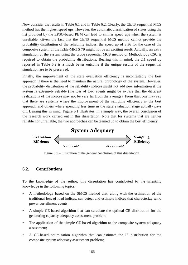
166

Now consider the results in Table 6.1 and in Table 6.2. Clearly, the CE/IS sequential MCS method has the highest speed ups. However, the automatic classification of states using the list provided by the EPSO-based PBM can lead to similar speed ups when the system is unreliable. Given the fact that the CE/IS sequential MCS method cannot provide the probability distribution of the reliability indices, the speed up of 3.36 for the case of the composite system of the IEEE-MRTS 79 might not be an exciting result. Actually, an extra simulation of the system using the crude sequential MCS method or Methodology CSC is required to obtain the probability distributions. Bearing this in mind, the 2.1 speed up reported in Table 6.2 is a much better outcome if the unique results of the sequential simulation are to be preserved.

Finally, the improvement of the state evaluation efficiency is incontestably the best approach if there is the need to maintain the natural chronology of the system. However, the probability distribution of the reliability indices might not add new information if the system is extremely reliable (the loss of load events might be so rare that the different realizations of the indices may not be very far from the average). From this, one may say that there are systems where the improvement of the sampling efficiency is the best approach and others where spending less time in the state evaluation stage actually pays off. Bearing this in mind, Figure 6.1 illustrates, in a simple way, the overall conclusion of the research work carried out in this dissertation. Note that for systems that are neither reliable nor unreliable, the two approaches can be teamed up to obtain the best efficiency.

Figure 6.1 – Illustration of the general conclusion of this dissertation.

6.2. Contributions

To the knowledge of the author, this dissertation has contributed to the scientific knowledge in the following topics:

• A methodology based on the SMCS method that, along with the estimation of the traditional loss of load indices, can detect and estimate indices that characterize wind power curtailment events;

• A simple CE-based algorithm that can calculate the optimal CE distribution for the generating capacity adequacy assessment problem;

• The application of the simple CE-based algorithm to the composite system adequacy assessment;

• A CE-based optimization algorithm that can estimate the IS distribution for the composite system adequacy assessment problem;

167

• The use of CE-based algorithms and IS with the SMCS method to the adequacy assessment of the composite system;

• The analysis and identification of the best modeling strategies in the CE-based algorithms for the time-dependent capacity of the generating units;

• The use of the list of states provided by the PBMs to intelligently categorize the states sampled by the sequential MCS method;

• The analysis and identification of the modeling strategy for the time-dependent capacity of the generating units in the PBMs that provide the most accurate estimates of the annual reliability indices as well as the highest speed ups of the SMCS method.

6.3. Perspectives of Future Research

Given the broad scope of research topics addressed in this dissertation, it is possible to propose a substantial number of research opportunities that might inspire other authors. As such, the following lines of research for the research topic addressed in Chapter 3 can be identified:

• Evaluation of the wind curtailment indices for a real power system;

• Analysis of the wind power curtailment events under a full AC representation;

• Development of an enhanced model that can automatically detect the amount of inertial load that must-run units have to supply as a function of the type of units in the up state;

• The detection of the benefits and drawbacks of using storing strategies for the wind energy not used on the long-term adequacy of the composite system.

As for the use of the CE method and IS technique to improve the sampling efficiency of the sequential MCS method, one has identified the following research opportunity:

• Development of methodology based on the CE/IS SMCS method that can provide accurate probability distributions for the reliability indices.

In addition to this stimulating research topic, there are other interesting applications of the CE method that need to be made, namely:

• Application CE/IS SMCS method in the evaluation of the well-being of the generating capacity and of the composite system;

• Application CE/IS SMCS method in the long-term adequacy assessment of the operating reserve;

Despite the good results reported by the methodology proposed in Chapter 5, the classification process based on the list provided by the PBMs is in an incipient stage. Consequently, there is extensive research that can be done regarding the application of PBMs to speed up the SMCS method, such as:

168

• Application of the Methodologies CSA, CSB and CSC in the composite system adequacy assessment of a real power system;

• Development of a new methodology that can merge the benefits of Methodology CSB and CSC, i.e., that can keep the speed ups of Methodology CSB and be applied to all composite systems;

• Using the EPSO-based PBM to train a pattern recognition technique, like the ANN or GMDH, to test if these techniques can replace in an efficient way the classification process made by the list of states.

Finally, the last topic of research proposed in this section consists of combining the classification methodologies proposed in Chapter 5 with the CE/IS SMCS method to create a hybrid methodology which will hopefully obtain even better speed ups over the crude SMCS method.

169

References

[1] “Europe 2020 Targets.” [Online]. Available: http://ec.europa.eu/europe2020/europe-2020-in-a-nutshell/targets/index_en.htm. [Accessed: 10-Feb-2013].

[2] R. N. Allan and R. Billinton, Reliability Evaluation of Power Systems, 2nd ed. Plenum Press, 1996.

[3] R. N. Allan, R. Li, and M. M. Elkateb, “Modelling of pumped-storage generation in sequential Monte Carlo production simulation,” IEE Proceedings Generation, Transmission and Distribution, vol. 145, no. 5, pp. 611–615, Sep. 1998.

[4] W. Wangdee, L. Wenyuan, and R. Billinton, “Coordinating wind and hydro generation to increase the effective load carrying capability,” in Proceedings of the 11th IEEE International Conference on Probabilistic Methods Applied to Power Systems (PMAPS), Singapore, 14-17 Jun. 2010.

[5] M. V. F. Pereira and N. J. Balu, “Composite generation/transmission reliability evaluation,” Proceedings of the IEEE, vol. 80, no. 4, pp. 470–491, Apr. 1992.

[6] A. M. Leite da Silva, L. A. F. Manso, and G. J. Anders, “Composite reliability evaluation for large-scale power systems,” in Proceedings of the IEEE Power Tech Conference (PowerTech), Bologna, Italy, 23-26 Jun. 2003

[7] A. M. Leite da Silva, R. A. González-Fernández, and C. Singh, “Generating capacity reliability evaluation based on Monte Carlo simulation and Cross-Entropy methods,” IEEE Transactions on Power Systems, vol. 25, no. 1, pp. 129–137, Feb. 2010.

[8] R. A. González-Fernández and A. M. Leite da Silva, “Reliability assessment of time-dependent systems via sequential Cross-Entropy Monte Carlo simulation,” IEEE Transactions on Power Systems, vol. 26, no. 4, pp. 2381–2389, Nov. 2011.

[9] R. Billinton and W. Li, Reliability Assessment of Electric Power Systems using Monte Carlo Methods. New York: Plenum Press, 1994.

[10] R. Y. Rubinstein and D. P. Kroese, Simulation and the Monte Carlo method, 2nd ed. John Wiley & Sons, Inc., 2008.

[11] A. M. Leite da Silva, A. C. G. Melo, and S. H. F. Cunha, “Frequency and duration method for reliability evaluation of large-scale hydrothermal generating systems,” IEE Proceedings Generation, Transmission and Distribution, vol. 138, no. 1, pp. 94–102, Jan. 1991.

170

[12] A. Sankarakrishnan and R. Billinton, “Sequential Monte Carlo simulation for composite power system reliability analysis with time varying loads,” IEEE Transactions on Power Systems, vol. 10, no. 3, pp. 1540–1545, Aug. 1995.

[13] N. Gubbala and C. Singh, “Models and considerations for parallel implementation of Monte Carlo simulation methods for power system reliability evaluation,” IEEE Transactions on Power Systems, vol. 10, no. 2, pp. 779–787, May 1995.

[14] C. L. T. Borges, D. M. Falcao, J. C. O. Mello, and A. C. G. Melo, “Composite reliability evaluation by sequential Monte Carlo simulation on parallel and distributed processing environments,” IEEE Transactions on Power Systems, vol. 16, no. 2, pp. 203–209, May 2001.

[15] G. Hager and G. Wellein, Introduction to High Performance Computing for Scientists and Engineers. CRC Press: Francis & Taylor Group, 2011.

[16] J. A. Silva Dias and C. L. T. Borges, “Object oriented model for composite reliability evaluation including time varying load and wind generation,” in Proceedings of the 11th IEEE International Conference on Probabilistic Methods Applied to Power Systems (PMAPS), Singapore, 14-17 Jun. 2010.

[17] H. M. Deitel and P. J. Deitel, JavaTM How To Program, 8th ed. Pearson Education, 2010.

[18] M. A. da Rosa, V. Miranda, L. M. Carvalho, and A. M. Leite da Silva, “Modern computing environment for power system reliability assessment,” in Proceedings of the 11th IEEE International Conference on Probabilistic Methods Applied to Power Systems (PMAPS), Singapore, 14-17 Jun. 2010.

[19] M. A. da Rosa, A. M. Leite da Silva, and V. Miranda, “Multi-agent systems applied to reliability assessment of power systems,” International Journal of Electrical Power & Energy Systems, vol. 42, no. 1, pp. 367–374, Nov. 2012.

[20] M. Wooldridge and N. R. Jennings, “Intelligent agents: Theory and practice,” Knowledge Engineering Review, pp. 115–152, 1995.

[21] M. A. da Rosa, “Agent-based Technology Applied to Power Systems Reliability,” Ph.D. dissertation, Faculty of Engineering of the University of Porto, Portugal, 2010.

[22] G. C. Oliveira, M. V. F. Pereira, and S. H. F. Cunha, “A technique for reducing computational effort in Monte-Carlo based composite reliability evaluation,” IEEE Transactions on Power Systems, vol. 4, no. 4, pp. 1309–1315, Nov. 1989.

[23] M. V. F. Pereira, M. E. P. Maceira, G. C. Oliveira, and L. M. V. G. Pinto, “Combining analytical models and Monte-Carlo techniques in probabilistic power system analysis,” IEEE Transactions on Power Systems, vol. 7, no. 1, pp. 265–272, Feb. 1992.

[24] H. Sy-Ruen and C. Shi-Lin, “Evaluation and improvement of variance reduction in Monte Carlo production simulation,” IEEE Transactions on Energy Conversion, vol. 8, no. 4, pp. 610–620, Dec. 1993.

[25] M. V. F. Pereira and L. M. V. G. Pinto, “A new computational tool for composite reliability evaluation,” IEEE Transactions on Power Systems, vol. 7, no. 1, pp. 258–264, Feb. 1992.

171

[26] P. T. de Boer, D. P. Kroese, S. Mannor, and R. Y. Rubinstein, “A tutorial on the Cross-Entropy Method,” Annals of Operations Research, vol. 134, no. 1, pp. 16–67, Jan. 2005.

[27] N. Amjady and M. Ehsan, “Evaluation of power systems reliability by an artificial neural network,” IEEE Transactions on Power Systems, vol. 14, no. 1, pp. 287–292, Feb. 1999.

[28] X. Luo, C. Singh, and A. D. Patton, “Using self-organizing map in identification of load-loss state,” in Proceedings of the International Conference on Electric Power Engineering (PowerTech), Budapest, Hungary, Aug. 29 - Sep. 2 1999.

[29] A. M. Leite da Silva, L. C. Resende, L. A. F. Manso, and V. Miranda, “Composite reliability assessment based on Monte Carlo simulation and artificial neural networks,” IEEE Transactions on Power Systems, vol. 22, no. 3, pp. 1202–1209, Aug. 2007.

[30] N. M. Pindoriya, P. Jirutitijaroen, D. Srinivasan, and C. Singh, “Composite reliability evaluation using Monte Carlo simulation and Least Squares Support Vector classifier,” IEEE Transactions on Power Systems, vol. 26, no. 4, pp. 2483–2490, Nov. 2011.

[31] C. M. Bishop, Pattern Recognition and Machine Learning (Information Science and Statistics). New York: Springer-Verlag Inc., 2006.

[32] N. Samaan and C. Singh, “Adequacy assessment of power system generation using a modified simple genetic algorithm,” IEEE Transactions on Power Systems, vol. 17, no. 4, pp. 974–981, Nov. 2002.

[33] L. Wang and C. Singh, “Population-based intelligent search in reliability evaluation of generation systems with wind power penetration,” IEEE Transactions on Power Systems, vol. 23, no. 3, pp. 1336–1345, Aug. 2008.

[34] V. Miranda, L. M. Carvalho, M. A. da Rosa, A. M. Leite da Silva, and C. Singh, “Improving power system reliability calculation efficiency with EPSO variants,” IEEE Transactions on Power Systems, vol. 24, no. 4, pp. 1772–1779, Nov. 2009.

[35] A. P. Engelbrecht, Computational Intelligence: An Introduction. Wiley Publishing, 2007.

[36] Thomas Bäck, Evolutionary Algorithms in Theory and Practice: Evolution Strategies, Evolutionary Programming, Genetic Algorithms. Oxford University Press, 1996.

[37] E. Alba, Parallel Metaheuristics: A New Class of Algorithms. John Wiley & Sons, Inc., 2005.

[38] M. Clerc and J. Kennedy, “The particle swarm - explosion, stability, and convergence in a multidimensional complex space,” IEEE Transactions on Evolutionary Computation, vol. 6, no. 1, pp. 58–73, Feb. 2002.

[39] D. Lieber, A. Nemirovskii, and R. Y. Rubinstein, “A fast Monte Carlo method for evaluating reliability indexes,” IEEE Transactions on Reliability, vol. 48, no. 3, pp. 256–261, Sep. 1999.

[40] R. A. González-Fernández, “Avaliação da Confiabilidade da Capacidade de Geração via o Método da Entropia Cruzada (in Portuguese),” M.Sc. Thesis, Federal University of Itajubá, MG, Brazil, 2009.

172

[41] R. A. González-Fernández, “Aplicações do Método da Entropia Cruzada na Confiabilidade de Sistemas Elétricos de Potência (in Portuguese),” Ph.D. dissertation, Federal University of Itajubá, MG, Brazil, 2012.

[42] P. Duhamel and M. Vetterli, “Fast Fourier transforms: A tutorial review and a state of the art,” Signal Processing, vol. 19, no. 4, pp. 259 – 299, Apr. 1990.

[43] F. F. Wu, Y.-K. Tsai, and Y.-X. Yu, “Probabilistic steady-state and dynamic security assessment,” IEEE Transactions on Power Systems, vol. 3, no. 1, pp. 1–9, Feb. 1988.

[44] F. F. Wu and Y.-K. Tsai, “Probabilistic dynamic security assessment of power systems-I: Basic model,” IEEE Transactions on Circuits and Systems, vol. 30, no. 3, pp. 148–159, Mar. 1983.

[45] A. M. Leite da Silva, J. Endrenyi, and L. Wang, “Integrated treatment of adequacy and security in bulk power system reliability evaluations,” IEEE Transactions on Power Systems, vol. 8, no. 1, pp. 275–285, Feb. 1993.

[46] R. Billinton and E. Khan, “A security based approach to composite power system reliability evaluation,” IEEE Transactions on Power Systems, vol. 7, no. 1, pp. 65–72, Feb. 1992.

[47] A. M. Rei, A. M. Leite da Silva, J. L. Jardim, and J. C. O. Mello, “Static and dynamic aspects in bulk power system reliability evaluations,” IEEE Transactions on Power Systems, vol. 15, no. 1, pp. 189–195, Feb. 2000.

[48] W. H. Press, S. A. Teukolsky, W. T. Vetterling, and B. P. Flannery, Numerical Recipes: The Art of Scientific Computing, 3rd ed. Cambridge University Press, 2007.

[49] H. Vasconcelos and J. A. Peças Lopes, “ANN design for fast security evaluation of interconnected systems with large wind power production,” in Proceedings of the 9th IEEE International Conference on Probabilistic Methods Applied to Power Systems (PMAPS), Stockholm, Sweden, 11-15 Jun. 2006.

[50] H. Kim and C. Singh, “Power system probabilistic security assessment using Bayes classifier,” Electric Power Systems Research, vol. 74, no. 1, pp. 157–165, Apr. 2005.

[51] S. Kalyani and K. S. Swarup, “Classification and assessment of power system security using multiclass SVM,” IEEE Transactions on Systems, Man, and Cybernetics, Part C: Applications and Reviews, vol. 41, no. 5, pp. 753–758, Sep. 2011.

[52] A. M. Leite da Silva, A. M. Cassula, R. Billinton, and L. A. F. Manso, “Integrated reliability evaluation of generation, transmission and distribution systems,” IEE Proceedings Generation, Transmission and Distribution, vol. 149, no. 1, pp. 1–6, Feb. 2002.

[53] M. A. Matos, J. A. Peças Lopes, M. A. da Rosa, R. Ferreira, A. M. Leite da Silva, W. Sales, L. Resende, L. A. F. Manso, P. Cabral, M. Ferreira, N. Martins, C. Artaiz, F. Soto, and R. López, “Probabilistic evaluation of reserve requirements of generating systems with renewable power sources: the Portuguese and Spanish cases,” International Journal of Electrical Power & Energy Systems, vol. 31, no. 9, pp. 562–569, Oct. 2009.

173

[54] A. M. Leite da Silva, W. S. Sales, L. A. F. Manso, and R. Billinton, “Long-term probabilistic evaluation of operating reserve requirements with renewable sources,” IEEE Transactions on Power Systems, vol. 25, no. 1, pp. 106–116, Feb. 2010.

[55] M. A. da Rosa, L. Bremermann, L. M. Carvalho, M. A. Matos, and M. Liquito, “Reserve Adequacy,” MERGE Project, Work Package 2, Task 2.5, Deliverable D2.2, 2012.

[56] L. Bremermann, M. A. da Rosa, M. A. Matos, J. A. Peças Lopes, and J. S. Akilimali, “Operating reserve assessment incorporating a stochastic electric vehicle model,” in Proceedings of the 12th IEEE International Conference on Probabilistic Methods Applied to Power Systems (PMAPS), Istanbul, Turkey, 10-14 Jun. 2012.

[57] M. A. Matos and R. J. Bessa, “Setting the operating reserve using probabilistic wind power forecasts,” IEEE Transactions on Power Systems, vol. 26, no. 2, pp. 594–603, May 2011.

[58] L. Guangbin and R. Billinton, “Operating reserve risk assessment in composite power systems,” IEEE Transactions on Power Systems, vol. 9, no. 3, pp. 1270–1276, Aug. 1994.

[59] R. Billinton, M. Fotuhi-Firuzabad, and S. Aboreshaid, “Unit commitment health analysis for interconnected systems,” IEEE Transactions on Power Systems, vol. 12, no. 3, pp. 1194–1201, Aug. 1997.

[60] M. Fotuhi-Firuzabad and R. Billinton, “Unit commitment health analysis in composite generation and transmission systems considering stand-by units,” IEE Proceedings Generation, Transmission and Distribution, vol. 146, no. 2, pp. 164–168, Mar. 1999.

[61] M. Fotuhi-Firuzabad and R. Billinton, “Impact of load management on composite system reliability evaluation short-term operating benefits,” IEEE Transactions on Power Systems, vol. 15, no. 2, pp. 858–864, May 2000.

[62] R. Billinton and J. Satish, “Predictive assessment of bulk-system-reliability performance indices,” IEE Proceedings Generation, Transmission and Distribution, vol. 141, no. 5, pp. 466–472, Sep. 1994.

[63] A. M. Leite da Silva, G. Perez A., J. W. Marangon Lima, and J. C. O. Mello, “Loss of load costs in generating capacity reliability evaluation,” Electric Power Systems Research, vol. 41, no. 2, pp. 109–116, May 1997.

[64] J. C. O. Mello, M. V. F. Pereira, A. M. Leite da Silva, and A. C. G. Melo, “Application of chronological load modeling in composite reliability worth evaluation,” Electric Power Systems Research, vol. 40, no. 3, pp. 167–174, Mar. 1997.

[65] R. Billinton and M. Fotuhi-Firuzabad, “A basic framework for generating system operating health analysis,” IEEE Transactions on Power Systems, vol. 9, no. 3, pp. 1610–1617, Aug. 1994.

[66] R. Billinton and R. Karki, “Application of Monte Carlo simulation to generating system well-being analysis,” IEEE Transactions on Power Systems, vol. 14, no. 3, pp. 1172–1177, Aug. 1999.

[67] L. Goel and C. Feng, “Well-being framework for composite generation and transmission system reliability evaluation,” IEE Proceedings Generation, Transmission and Distribution, vol. 146, no. 5, pp. 528–534, Sep. 1999.

174

[68] A. M. Leite da Silva, L. C. Resende, L. A. F. Manso, and R. Billinton, “Well-being analysis for composite generation and transmission systems,” IEEE Transactions on Power Systems, vol. 19, no. 4, pp. 1763–1770, Nov. 2004.

[69] L. Goel and R. Gupta, “Extending health considerations in subtransmission systems to include reliability worth,” IEE Proceedings Generation, Transmission and Distribution, vol. 147, no. 6, pp. 381–386, Nov. 2000.

[70] A. Abiri-Jahromi, M. Fotuhi-Firuzabad, and E. Abbasi, “Optimal scheduling of spinning reserve based on well-being model,” IEEE Transactions on Power Systems, vol. 22, no. 4, pp. 2048–2057, Nov. 2007.

[71] J. C. O. Mello, M. V. F. Pereira, and A. M. Leite da Silva, “Evaluation of reliability worth in composite systems based on pseudo-sequential Monte Carlo simulation,” IEEE Transactions on Power Systems, vol. 9, no. 3, pp. 1318–1326, Aug. 1994.

[72] S. H. F. Cunha, M. V. F. Pereira, L. M. V. G. Pinto, and G. C. Oliveira, “Composite generation and transmission reliability evaluation in large hydroelectric systems,” IEEE Transactions on Power Apparatus and Systems, vol. PAS-104, no. 10, pp. 2657–2663, Oct. 1985.

[73] R. N. Allan, A. M. Leite da Silva, A. A. Abu-Nasser, and R. C. Burchett, “Discrete convolution in power system reliability,” IEEE Transactions on Reliability, vol. R-30, no. 5, pp. 452–456, Dec. 1981.

[74] A. M. Leite da Silva, F. A. F. Pazo Blanco, and J. Coelho, “Discrete convolution in generating capacity reliability evaluation-LOLE calculations and uncertainty aspects,” IEEE Transactions on Power Systems, vol. 3, no. 4, pp. 1616–1624, Nov. 1988.

[75] N. S. Rau, P. Toy, and K. F. Schenk, “Expected energy production costs by the method of moments,” IEEE Transactions on Power Apparatus and Systems, vol. PAS-99, no. 5, pp. 1908–1917, Sep. 1980.

[76] M. M. Alavi-Sereshki and C. Singh, “A generalized continuous distribution approach for generating capacity reliability evaluation and its applications,” IEEE Transactions on Power Systems, vol. 6, no. 1, pp. 16–22, Feb. 1991.

[77] D. J. Levy and E. P. Kahn, “Accuracy of the Edgeworth approximation for LOLP calculations in small power systems,” IEEE Transactions on Power Apparatus and Systems, vol. PAS-101, no. 4, pp. 986–996, Apr. 1982.

[78] J. Usaola, “Probabilistic load flow in systems with wind generation,” IET Generation, Transmission & Distribution, vol. 3, no. 12, pp. 1031–1041, Dec. 2009.

[79] A. M. Leite da Silva, L. A. F. Manso, J. C. O. Mello, and R. Billinton, “Pseudo-chronological simulation for composite reliability analysis with time varying loads,” IEEE Transactions on Power Systems, vol. 15, no. 1, pp. 73–80, Feb. 2000.

[80] A. M. Leite da Silva, R. A. González-Fernández, W. S. Sales, and L. A. F. Manso, “Reliability assessment of time-dependent systems via quasi-sequential Monte Carlo simulation,” in Proceedings of the 11th IEEE International Conference on Probabilistic Methods Applied to Power Systems (PMAPS), Singapore, 14-17 Jun. 2010.

175

[81] S. M. Ross, Introduction to Probability Models, 10th ed. Academic Press, Inc., 2006.

[82] A. C. G. Melo, M. V. F. Pereira, and A. M. Leite da Silva, “Frequency and duration calculations in composite generation and transmission reliability evaluation,” IEEE Transactions on Power Systems, vol. 7, no. 2, pp. 469–476, May 1992.

[83] C. L. T. Borges, “An overview of reliability models and methods for distribution systems with renewable energy distributed generation,” Renewable and Sustainable Energy Reviews, vol. 16, no. 6, pp. 4008–4015, Aug. 2012.

[84] J. Grainger and William Stevenson Jr., Power System Analysis. McGraw-Hill Publishing Co., 1994.

[85] A. J. Wood and B. F. Wollenberg, Power Generation Operation and Control. John Wiley & Sons, Inc., 1996.

[86] A. S. Costa and R. Salgado, “Configurador de Redes (in Portuguese),” 2002. [Online]. Available: http://www.labspot.ufsc.br/~simoes/assp/assp8.pdf. [Accessed: 11-Feb-2013].

[87] J. C. Nash, “The (Dantzig) simplex method for linear programming,” Computing in Science & Engineering, vol. 2, no. 1, pp. 29–31, January-February 2000.

[88] J. Gondzio, “Interior point methods 25 years later,” European Journal of Operational Research, vol. 218, no. 3, pp. 587–601, May 2012.

[89] M. Berkelaar, J. Dirks, K. Eikland, P. Notebaert, J. Ebert, and H. Gourvest, “LP Solve - A Mixed Integer Linear Programming (MILP) solver.” [Online]. Available: http://lpsolve.sourceforge.net/5.5/. [Accessed: 17-Dec-2012].

[90] G. Dantzig and M. Thapa, Linear Programming 2: Theory and Extensions. Springer, 2006.

[91] P. M. Subcommittee, “IEEE Reliability Test System,” IEEE Transactions on Power Apparatus and Systems, vol. PAS-98, no. 6, pp. 2047–2054, Nov. 1979.

[92] C. Grigg, P. Wong, P. Albrecht, R. Allan, M. Bhavaraju, R. Billinton, Q. Chen, C. Fong, S. Haddad, S. Kuruganty, W. Li, R. Mukerji, D. Patton, N. Rau, D. Reppen, A. Schneider, M. Shahidehpour, and C. Singh, “The IEEE reliability test system-1996. A report prepared by the reliability test system task force of the application of probability methods subcommittee,” IEEE Transctions on Power Systems, vol. 14, no. 3, pp. 1010–1020, Aug. 1999.

[93] L. C. Resende, “Avaliação da confiabilidade preventiva de sistemas életricos de grande porte utilizando redes neurais (in Portuguese),” Ph.D. dissertation, Federal University of Itajubá, MG, Brazil, 2006.

[94] M. Amelin, “Comparison of capacity credit calculation methods for conventional power plants and wind power,” IEEE Transactions on Power Systems, vol. 24, no. 2, pp. 685–691, May 2009.

[95] J. Wen, Y. Zheng, and F. Donghan, “A review on reliability assessment for wind power,” Renewable and Sustainable Energy Reviews, vol. 13, no. 9, pp. 2485–2494, Dec. 2009.

176

[96] J. Haslett and M. Diesendorf, “The capacity credit of wind power: a theoretical analysis,” Solar Energy, vol. 26, no. 5, pp. 391–401, 1981.

[97] P. Giorsetto and K. F. Utsurogi, “Development of a new procedure for reliability modeling of wind turbine generators,” IEEE Transactions on Power Apparatus and Systems, vol. PAS-102, no. 1, pp. 134–143, Jan. 1983.

[98] R. Billinton and C. Hua, “Assessment of risk-based capacity benefit factors associated with wind energy conversion systems,” IEEE Transactions on Power Systems, vol. 13, no. 3, pp. 1191–1196, Aug. 1998.

[99] W. Wangdee and R. Billinton, “Considering load-carrying capability and wind speed correlation of WECS in generation adequacy assessment,” IEEE Transactions on Energy Conversion, vol. 21, no. 3, pp. 734–741, Sep. 2006.

[100] K. R. Voorspools and W. D. D’haeseleer, “An analytical formula for the capacity credit of wind power,” Renewable Energy, vol. 31, no. 1, pp. 45–54, Jan. 2006.

[101] R. Karki, “Renewable energy credit driven wind power growth for system reliability,” Electric Power Systems Research, vol. 77, no. 7, pp. 797–803, May 2007.

[102] K. Xie and R. Billinton, “Energy and reliability benefits of wind energy conversion systems,” Renewable Energy, vol. 36, no. 7, pp. 1983–1988, Jul. 2011.

[103] S. Zhu, Y. Zhang, and A. A. Chowdhury, “Capacity credit of wind generation based on minimum resource adequacy procurement,” IEEE Transactions on Industry Applications, vol. 48, no. 2, pp. 730–735, March-April 2012.

[104] L. L. Garver, “Effective load carrying capability of generating units,” IEEE Transactions on Power Apparatus and Systems, vol. PAS-85, no. 8, pp. 910–919, 1966.

[105] R. Karki, H. Po, and R. Billinton, “Reliability evaluation considering wind and hydro power coordination,” IEEE Transactions on Power Systems, vol. 25, no. 2, pp. 685–693, May 2010.

[106] B. Bagen and R. Billinton, “Incorporating well-being considerations in generating systems using energy storage,” IEEE Transactions on Energy Conversion, vol. 20, no. 1, pp. 225–230, Mar. 2005.

[107] R. Billinton and B. Bagen, “Incorporating reliability index distributions in small isolated generating system reliability performance assessment,” IEE Proceedings Generation, Transmission and Distribution, vol. 151, no. 4, pp. 469–476, Jun. 2004.

[108] R. Billinton, B. Karki, R. Karki, and G. Ramakrishna, “Unit commitment risk analysis of wind integrated power systems,” IEEE Transactions on Power Systems, vol. 24, no. 2, pp. 930–939, May 2009.

[109] P. Wang, Z. Gao, and L. Bertling, “Operational adequacy studies of power systems with wind farms and energy storages,” IEEE Transactions on Power Systems, vol. 27, no. 4, pp. 2377–2384, Nov. 2012.

[110] A. M. Leite da Silva, L. A. F. Manso, W. S. Sales, L. C. Resende, M. J. Q. Aguiar, M. A. Matos, J. A. P. Lopes, and V. Miranda, “Application of Monte Carlo simulation to

177

generating system well-being analysis considering renewable sources,” in Proceedings of the 9th IEEE International Conference on Probabilistic Methods Applied to Power Systems (PMAPS), Stockholm, Sweden, 11-15 Jun. 2006.

[111] R. Billinton and R. Karki, “Maintaining supply reliability of small isolated power systems using renewable energy,” IEE Proceedings Generation, Transmission and Distribution, vol. 148, no. 6, pp. 530–534, Nov. 2001.

[112] D. Huang and R. Billinton, “Effects of wind power on bulk system adequacy evaluation using the well-being analysis framework,” IEEE Transactions on Power Systems, vol. 24, no. 3, pp. 1232–1240, Aug. 2009.

[113] W. Wangdee and R. Billinton, “Probing the intermittent energy resource contributions from generation adequacy and security perspectives,” IEEE Transactions on Power Systems, vol. 27, no. 4, pp. 2306–2313, Nov. 2012.

[114] R. Billinton, G. Yi, and R. Karki, “Composite system adequacy assessment incorporating large-scale wind energy conversion systems considering wind speed correlation,” IEEE Transactions on Power Systems, vol. 24, no. 3, pp. 1375–1382, Aug. 2009.

[115] R. Billinton, R. Karki, Y. Gao, D. Huang, P. Hu, and W. Wangdee, “Adequacy assessment considerations in wind integrated power systems,” IEEE Transactions on Power Systems, vol. 27, no. 4, pp. 2297–2305, Nov. 2012.

[116] W. Wangdee and R. Billinton, “Reliability assessment of bulk electric systems containing large wind farms,” International Journal of Electrical Power & Energy Systems, vol. 29, no. 10, pp. 759–766, Dec. 2007.

[117] Y. Z. Y. Zhang, S. Z. S. Zhu, and A. A. Chowdhury, “Reliability modeling of a composite energy storage and wind generation systems with adequate transmission upgrades,” in Proceedings of the IEEE Power and Energy Society General Meeting, Minneapolis, MN, USA, 25-29 July 2010

[118] A. M. Leite da Silva, L. A. F. Manso, W. S. Sales, S. A. Flavio, G. J. Anders, and L. C. Resende, “Chronological power flow for planning transmission systems considering intermittent sources,” IEEE Transactions on Power Systems, vol. 27, no. 4, pp. 2314–2322, Nov. 2012.

[119] R. Billinton and W. Wangdee, “Reliability-based transmission reinforcement planning associated with large-scale wind farms,” IEEE Transactions on Power Systems, vol. 22, no. 1, pp. 34–41, Feb. 2007.

[120] F. Vallée, J. Lobry, and O. Deblecker, “Wind generation modelling to help the managerial process of modern transmission systems,” Renewable Energy, vol. 36, no. 5, pp. 1632–1638, May 2011.

[121] S. Fink, C. Mudd, K. Porter, and B. Morgenstern, “Wind energy curtailment case studies,” National Renewable Energy Laboratory, Rep. NREL/SR-550-46716, 2009.

[122] D. J. Burke and M. J. O’Malley, “Factors influencing wind energy curtailment,” IEEE Transactions on Sustainable Energy, vol. 2, no. 2, pp. 185–193, Apr. 2011.

178

[123] F. Castro Sayas and R. N. Allan, “Generation availability assessment of wind farms,” IEE Proceedings Generation, Transmission and Distribution, vol. 143, no. 5, pp. 507–518, Sep. 1996.

[124] IEC 61400-12-1, “Wind turbines - Part 12-1: Power performance measurements of electricity producing wind turbines.” 2005.

[125] T.-H. Yeh and L. Wang, “A study on generator capacity for wind turbines under various tower heights and rated wind speeds using weibull distribution,” IEEE Transactions on Energy Conversion, vol. 23, no. 2, pp. 592–602, Jun. 2008.

[126] X. Han, J. Guo, and P. Wang, “Adequacy study of a wind farm considering terrain and wake effect,” IET Generation, Transmission & Distribution, vol. 6, no. 10, pp. 1001–1008, Oct. 2012.

[127] A. P. Leite, C. L. T. Borges, and D. M. Falcao, “Probabilistic wind farms generation model for reliability studies applied to brazilian sites,” IEEE Transactions on Power Systems, vol. 21, no. 4, pp. 1493–1501, Nov. 2006.

[128] R. Billinton and D. Huang, “Incorporating wind power in generating capacity reliability evaluation using different models,” IEEE Transactions on Power Systems, vol. 26, no. 4, pp. 2509–2517, Nov. 2011.

[129] R. Billinton, H. Chen, and R. Ghajar, “Time-series models for reliability evaluation of power systems including wind energy,” Microelectronics Reliability, vol. 36, no. 9, pp. 1253–1261, Sep. 1996.

[130] P. Chen, T. Pedersen, B. Bak-Jensen, and Z. Chen, “ARIMA-based time series model of stochastic wind power generation,” IEEE Transactions on Power Systems, vol. 25, no. 2, pp. 667–676, May 2010.

[131] A. Shamshad, M. A. Bawadi, W. M. A. Wan Hussin, T. A. Majid, and S. A. M. Sanusi, “First and second order Markov chain models for synthetic generation of wind speed time series,” Energy, vol. 30, no. 5, pp. 693–708, Apr. 2005.

[132] G. Papaefthymiou and B. Klockl, “MCMC for wind power simulation,” IEEE Transactions on Energy Conversion, vol. 23, no. 1, pp. 234–240, Mar. 2008.

[133] G. D’Amico, F. Petroni, and F. Prattico, “Reliability measures of second-order semi-Markov chain applied to wind energy production,” Journal of Renewable Energy, vol. 2013, 2013.

[134] R. Billinton, C. Hua, and R. Ghajar, “A sequential simulation technique for adequacy evaluation of generating systems including wind energy,” IEEE Transactions on Energy Conversion, vol. 11, no. 4, pp. 728–734, Dec. 1996.

[135] B. Hasche, A. Keane, and M. O’Malley, “Capacity value of wind power, calculation, and data requirements: the Irish power system case,” IEEE Transactions on Power Systems, vol. 26, no. 1, pp. 420–430, Feb. 2011.

[136] R. Billinton and Y. Gao, “Multistate wind energy conversion system models for adequacy assessment of generating systems incorporating wind energy,” IEEE Transactions on Energy Conversion, vol. 23, no. 1, pp. 163–170, Mar. 2008.

179

[137] A. S. Dobakhshari and M. Fotuhi-Firuzabad, “A reliability model of large wind farms for power system adequacy studies,” IEEE Transactions on Energy Conversion, vol. 24, no. 3, pp. 792–801, Sep. 2009.

[138] C. Singh and Y. Kim, “An efficient technique for reliability analysis of power systems including time dependent sources,” IEEE Transactions on Power Systems, vol. 3, no. 3, pp. 1090–1096, Aug. 1988.

[139] H. Kim, C. Singh, and A. Sprintson, “Simulation and estimation of reliability in a wind farm considering the wake effect,” IEEE Transactions on Sustainable Energy, vol. 3, no. 2, pp. 274–282, Apr. 2012.

[140] P. Didsayabutra, L. Wei-Jen, and B. Eua-Arporn, “Defining the must-run and must-take units in a deregulated market,” IEEE Transactions on Industry Applications, vol. 38, no. 2, pp. 596–601, March-April 2002.

[141] G. Pritchard, “The must-run dispatch auction in an electricity market,” Energy Economics, vol. 24, no. 3, pp. 199–216, May 2002.

[142] P. Jirutitijaroen and C. Singh, “Comparison of simulation methods for power system reliability indexes and their distributions,” IEEE Transactions on Power Systems, vol. 23, no. 2, pp. 486–493, May 2008.

[143] R. Billinton and Jonnavithula, “Composite system adequacy assessment using sequential Monte Carlo simulation with variance reduction techniques [power networks],” IEE Proceedings Generation, Transmission and Distribution, vol. 144, no. 1, pp. 1–6, Jan. 1997.

[144] U. Küchler and M. Sørensen, “Exponential families of stochastic processes and Lévy processes,” Journal of Statistical Planning and Inference, vol. 39, no. 2, pp. 211–237, Apr. 1994.

[145] A. Shandilya, H. Gupta, and J. Sharma, “Method for generation rescheduling and load shedding to alleviate line overloads using local optimisation,” IEE Proceedings Generation, Transmission and Distribution, vol. 140, no. 5, pp. 337–342, Sep. 1993.

[146] M. K. Enns, J. J. Quada, and B. Sackett, “Fast linear contingency analysis,” IEEE Transactions on Power Apparatus and Systems, vol. PAS-101, no. 4, pp. 783–791, Apr. 1982.

[147] S. A. Farghal, M. A. Tantawy, M. S. A. Hussien, S. A. Hassan, and A. A. A. Elela, “Fast technique for power system security assessment using sensitivity parameters of linear programming,” IEEE Transactions on Power Apparatus and Systems, vol. PAS-103, no. 5, pp. 946–953, May 1984.

[148] M. E. Khan and R. Billinton, “A hybrid model for quantifying different operating states of composite power systems,” IEEE Transactions on Power Systems, vol. 7, no. 1, pp. 187–193, Feb. 1992.

[149] S. Jonnavithula and R. Billinton, “Topological analysis in bulk power system reliability evaluation,” IEEE Transactions on Power Systems, vol. 12, no. 1, pp. 456–463, Feb. 1997.

[150] J. B. Ward, “Equivalent circuits for power-flow studies,” Transactions of the American Institute of Electrical Engineers, vol. 68, no. 1, pp. 373–382, Sep. 1949.

180

[151] V. Miranda and N. Fonseca, “EPSO best-of-two-worlds meta-heuristic applied to power system problems,” in Proceedings of the Congress on Evolutionary Computation (CEC), Honolulu, HI, USA, May 12-17 2002.

[152] G. Yongji, X. Yongjian, X. Kai, and Y. Huiyi, “Composite system reliability evaluation based on Monte-Carlo simulation combined with outages screening,” IEEE Transactions on Power Systems, vol. 14, no. 2, pp. 785–790, May 1999.

[153] D. H. Wolpert and W. G. Macready, “No free lunch theorems for optimization,” IEEE Transactions on Evolutionary Computation, vol. 1, no. 1, pp. 67–82, May 1997.

[154] A. E. Eiben and C. A. Schippers, “On evolutionary exploration and exploitation,” Fundamenta Informaticae, vol. 35, no. 1–4, pp. 35–50, 1998.

[155] N. Mladenovic and P. Hansen, “Variable neighborhood search,” Computers & Operations Research, vol. 24, no. 11, pp. 1097–1100, Nov. 1997.

[156] B. Suman and P. Kumar, “A survey of simulated annealing as a tool for single and multiobjective optimization,” Journal of the Operational Research Society, vol. 57, no. 10, pp. 1143–1160, Oct. 2006.

[157] T. Feo and M. Resende, “Greedy randomized adaptive search procedures,” Journal of Global Optimization, vol. 6, no. 2, pp. 109–133, Mar. 1995.

[158] F. Glover, “Tabu Search: A tutorial,” Interfaces, vol. 20, no. 4, pp. 74–94, Jul. 1990.

[159] S. Das and P. . Suganthan, “Differential Evolution: A survey of the state-of-the-art,” IEEE Transactions on Evolutionary Computation, vol. 15, no. 1, pp. 4–31, Feb. 2011.

[160] M. Dorigo, V. Maniezzo, and A. Colorni, “The Ant System: Optimization by a colony of cooperating agents,” IEEE Transactions on Systems, Man, and Cybernetics Part B: Cybernetics, vol. 26, no. 1, pp. 29–41, Feb. 1996.

[161] J. Farmer, N. Packard, and A. Perelson, “The immune system, adaptation, and machine learning,” Physica D: Nonlinear Phenomena, vol. 22, no. 1–3, pp. 187–204, Oct. 1986.

[162] D. Karaboga and B. Basturk, “On the performance of artificial bee colony (ABC) algorithm,” Applied Soft Computing, vol. 8, no. 1, pp. 687–697, Jan. 2008.

[163] C. Savage, “A survey of combinatorial Gray codes,” SIAM Review, vol. 39, no. 4, pp. 605–629, Dec. 1997.

[164] K. Deb and D. Kalyanmoy, Multi-Objective Optimization Using Evolutionary Algorithms. John Wiley & Sons, Ltd., 2001.

[165] E. Zitzler and L. Thiele, “An Evolutionary Algorithm for Multiobjective Optimization: The Strength Pareto Approach,” TIK-Report 43, Federal Institute of Technology, Zurich, Switzerland, May 1998.

[166] E. Zitzler, M. Laumanns, and L. Thiele, “SPEA2: Improving the Strength Pareto Evolutionary Algorithm,” TIK-Report 103, Zurich, Federal Institute of Technology, Switzerland, May 2001.

181

[167] C. A. Coello Coello and M. S. Lechuga, “MOPSO: A proposal for multiple objective particle swarm optimization,” in in Proceedings of the Congress on Evolutionary Computation (CEC), Honolulu, HI, USA, May 12-17 2002.

[168] C. A. Coello Coello, G. T. Pulido, and M. S. Lechuga, “Handling multiple objectives with particle swarm optimization,” IEEE Transactions on Evolutionary Computation,, vol. 8, no. 3, pp. 256–279, Jun. 2004.

[169] R. S. Maciel, M. A. da Rosa, V. Miranda, and A. Padilha-Feltrin, “Multi-objective evolutionary particle swarm optimization in the assessment of the impact of distributed generation,” Electric Power Systems Research, vol. 89, no. 0, pp. 100–108, Aug. 2012.

[170] V. Miranda, H. Keko, and A. Duque, “Stochastic star communication topology in evolutionary particle swarms (EPSO),” International Journal of Computational Intelligence Research, vol. 4, no. 2, pp. 105–116, 2008.

[171] R. C. Green, L. Wang, M. Alam, and C. Singh, “Intelligent state space pruning using multi-objective PSO for reliability analysis of composite power systems: Observations, analyses, and impacts,” in Proceedings of the IEEE Power and Energy Society General Meeting, Chicago, IL, USA, 24 – 28 July 2011.

[172] R. C. Green, L. Wang, M. Alam, and C. Singh, “State space pruning for reliability evaluation using binary particle swarm optimization,” in Proceedings of the IEEE Power Systems Conference and Exposition (PSCE), Phoenix, AZ, USA, 20-23 March 2011

[173] N. Samaan and C. Singh, “Genetic algorithms approach for the evaluation of composite generation-transmission systems reliability worth,” in Proceedings of the IEEE PES Transmission and Distribution Conference and Exposition, Dallas, TX, USA, 7-12 Sept. 2003.

[174] N. Samaan and C. Singh, “Assessment of the annual frequency and duration indices in composite system reliability using genetic algorithms,” in Proceedings of the IEEE Power and Energy Society General Meeting, Toronto, Canada, 13-17 July 2003.

[175] M. R. Gholami, S. H. Hoseini, and M. Mohamad Taheri, “Assessment of power composite system annualized reliability indices based on improved particle swarm optimization and comparative study between the behaviour of GA and PSO,” in Proceedings of the 2nd IEEE International Power and Energy Conference (PECon), Johor Bahru, Malaysia, 1-3 Dec. 2008.

[176] R. C. Green, W. Lingfeng, and C. Singh, “State space pruning for power system reliability evaluation using genetic algorithms,” in Proceedings of the IEEE Power and Energy Society General Meeting, Minneapolis, MN, USA, 25-29 July 2010.

[177] W. McAllister, Data Structures and Algorithms Using Java. Jones & Bartlett Publishers, 2008.

[178] R. Bellman, Dynamic Programming. Dover Publications Inc., 2003.

182

183

Appendix A - List of Publications

Publications in Peer Reviewed Journals

• V. Miranda, L. M. Carvalho , M. A. da Rosa, A. M. Leite da Silva, and C. Singh, “Improving power system reliability calculation efficiency with EPSO variants,” IEEE Transactions on Power Systems, vol. 24, no. 4, pp. 1772–1779, Nov. 2009.

• J. Wang, A. Botterud, R. Bessa, H. Keko, L. M. Carvalho , D. Issicaba, J. Sumaili, and V. Miranda, “Wind power forecasting uncertainty and unit commitment,” Applied Energy, vol. 88, no. 11, pp. 4014–4023, Nov. 2011.

• L. M. Carvalho , M. A. da Rosa, A. M. Leite da Silva, and V. Miranda, “Probabilistic analysis for maximizing the grid integration of wind power generation,” IEEE Transactions on Power Systems, vol. 27, no. 4, pp. 2323–2331, Nov. 2012.

• L. M. Carvalho , R. A. Gonzalez-Fernandez, A. M. Leite da Silva, M. A. da Rosa, and V. Miranda, “Simplified Cross-Entropy Based Approach for Generating Capacity Reliability Assessment,” IEEE Transactions on Power Systems, 2012 (in press).

Publications in Peer Reviewed Conferences

• M. A. da Rosa, V. Miranda, L. M. Carvalho , and A. M. Leite da Silva, “Modern computing environment for power system reliability assessment,” in Proceedings of the IEEE International Conference on Probabilistic Methods Applied to Power Systems (PMAPS), Singapore, 14-17 Jun. 2010.

• L. M. Carvalho , M. A. da Rosa, V. Miranda, and R. Ferreira, “A chronological composite system adequacy assessment considering non-dispatchable renewable energy sources and their integration strategies,” in Proceedings of the 17th Power Systems Computation Conference (PSCC’11), Stockholm, Sweden, 22-26 Aug. 2011.

• L. M. Carvalho , D. Issicaba, M. A. da Rosa, J. P. V. Ramos, and V. Miranda, “Reliability evaluation of generation systems via sequential Population-based Monte Carlo simulation,” in Proceedings of the 12th IEEE International Conference on Probabilistic Methods Applied to Power Systems (PMAPS), Istanbul, Turkey, 10-14 Jun. 2012.

• L. Bremermann, L. M. Carvalho , M. A. da Rosa, M. Matos, J. A. Peças Lopes, “Avaliação do Risco da Integração de Veículos Elétricos na Adequação da Reserva

184

Operacional,” Encontro Nacional de Riscos, Segurança e Fiabilidade (ENRSF), Lisbon, Portugal, 15-17 May 2012. (in Portuguese)

Technical Reports

• M. A. da Rosa, L. Bremermann, L. M. Carvalho , M. Matos, M. Liquito, “Reserve Adequacy,” MERGE Project, Work Package 2, Task 2.5, Deliverable D2.2, Feb. 2011.

• M. A. da Rosa, L. Bremermann, I. Costa, L. M. Carvalho , “Static and operational reserve adequacy of Portugal, Spain and Greece power systems,” MERGE Project, Work Package 4, Task 4.2, Deliverable D4.2, Jan. 2012.

• INESC Porto, “Desenvolvimento de Ferramentas de Análise do Impacto Técnico da Integração de Microprodução e Veículos Eléctricos,” REIVE Project, Apr. 2012. (in Portuguese)

• M. A. da Rosa, L. M. Carvalho , I. Costa, “Avaliação Probabilística da Adequação dos Sistemas de Geração e Transporte da Ilha da Madeira Incluindo a Minimização do Desperdício de Energia Renovável,” Aug. 2012. (in Portuguese)

A new paper, which will be submitted to the IEEE Transactions on Power Systems, is being developed with the research reported in Chapter 5.