Adversarial Transformation Networks: Learning to Generate

Adversarial Transformation Networks:Learning to Generate Adversarial Examples

Shumeet Baluja and Ian FischerGoogle Research

Mountain View, CA.

Abstract

Multiple different approaches of generating ad-versarial examples have been proposed to attackdeep neural networks. These approaches involveeither directly computing gradients with respectto the image pixels, or directly solving an op-timization on the image pixels. In this work,we present a fundamentally new method for gen-erating adversarial examples that is fast to exe-cute and provides exceptional diversity of out-put. We efficiently train feed-forward neural net-works in a self-supervised manner to generateadversarial examples against a target network orset of networks. We call such a network an Ad-versarial Transformation Network (ATN). ATNsare trained to generate adversarial examples thatminimally modify the classifier’s outputs giventhe original input, while constraining the newclassification to match an adversarial target class.We present methods to train ATNs and analyzetheir effectiveness targeting a variety of MNISTclassifiers as well as the latest state-of-the-art Im-ageNet classifier Inception ResNet v2.

1. Introduction and BackgroundWith the resurgence of deep neural networks for many real-world classification tasks, there is an increased interest inmethods to generate training data, as well as to find weak-nesses in trained models. An effective strategy to achieveboth goals is to create adversarial examples that trainedmodels will misclassify. Adversarial examples are smallperturbations of the inputs that are carefully crafted to foolthe network into producing incorrect outputs. These smallperturbations can be used both offensively, to fool modelsinto giving the “wrong” answer, and defensively, by pro-viding training data at weak points in the model. Semi-nal work by Szegedy et al. (2013) and Goodfellow et al.

(2014b), as well as much recent work, has shown that ad-versarial examples are abundant, and that there are manyways to discover them.

Given a classifier f(x) : x ∈ X → y ∈ Y and orig-inal inputs x ∈ X , the problem of generating untar-geted adversarial examples can be expressed as the opti-mization: argminx∗ L(x,x∗) s.t. f(x∗) 6= f(x), whereL(·) is a distance metric between examples from the in-put space (e.g., the L2 norm). Similarly, generating a tar-geted adversarial attack on a classifier can be expressed asargminx∗ L(x,x∗) s.t. f(x∗) = yt, where yt ∈ Y is sometarget label chosen by the attacker.1

Until now, these optimization problems have been solvedusing three broad approaches: (1) By directly using opti-mizers like L-BFGS or Adam (Kingma & Ba, 2015), asproposed in Szegedy et al. (2013) and Carlini & Wag-ner (2016). Such optimizer-based approaches tend to bemuch slower and more powerful than the other approaches.(2) By approximation with single-step gradient-based tech-niques like fast gradient sign (Goodfellow et al., 2014b)or fast least likely class (Kurakin et al., 2016a). These ap-proaches are fast, requiring only a single forward and back-ward pass through the target classifier to compute the per-turbation. (3) By approximation with iterative variants ofgradient-based techniques (Kurakin et al., 2016a; Moosavi-Dezfooli et al., 2016a;b). These approaches use multipleforward and backward passes through the target network tomore carefully move an input towards an adversarial clas-sification.

1Another axis to compare when considering adversarial at-tacks is whether the adversary has access to the internals of the tar-get model. Attacks without internal access are possible by trans-ferring successful attacks on one model to another model, as inSzegedy et al. (2013); Papernot et al. (2016a), and others. A morechallenging class of blackbox attacks involves having no accessto any relevant model, and only getting online access to the tar-get model’s output, as explored in Papernot et al. (2016b); Balujaet al. (2015); Tramer et al. (2016). See Papernot et al. (2015) fora detailed discussion of threat models.

arX

iv:1

703.

0938

7v1

[cs

.NE

] 2

8 M

ar 2

017

Adversarial Transformation Networks

2. Adversarial Transformation NetworksIn this work, we propose Adversarial Transformation Net-works (ATNs). An ATN is a neural network that transformsan input into an adversarial example against a target net-work or set of networks. ATNs may be untargeted or tar-geted, and trained in a black-box2 or white-box manner. Inthis work, we will focus on targeted, white-box ATNs.

Formally, an ATN can be defined as a neural network:

gf,θ(x) : x ∈ X → x′ (1)

where θ is the parameter vector of g, f is the target networkwhich outputs a probability distribution across class labels,and x′ ∼ x, but argmax f(x) 6= argmax f(x′).

Training. To find gf,θ, we solve the following optimiza-tion:

argminθ

∑xi∈X

βLX (gf,θ(xi),xi)+LY(f(gf,θ(xi)), f(xi))

(2)where LX is a loss function in the input space (e.g., L2 lossor a perceptual similarity loss like Johnson et al. (2016)),LY is a specially-formed loss on the output space of f (de-scribed below) to avoid learning the identity function, andβ is a weight to balance the two loss functions. We willomit θ from gf when there is no ambiguity.

Inference. At inference time, gf can be run on any inputx without requiring further access to f or more gradientcomputations. This means that after being trained, gf cangenerate adversarial examples against the target network feven faster than the single-step gradient-based approaches,such as fast gradient sign, so long as ||gf || / ||f ||.

Loss Functions. The input-space loss function, LX ,would ideally correspond closely to human perception.However, for simplicity, L2 is sufficient. LY determineswhether or not the ATN is targeted; the target refers to theclass for which the adversary will cause the classifier tooutput the maximum value. In this work, we focus on themore challenging case of creating targeted ATNs, whichcan be defined similarly to Equation 1:

gf,t(x) : x ∈ X → x′ (3)

where t is the target class, so that argmax f(x′) = t. Thisallows us to target the exact class the classifier should mis-takenly believe the input is.

In this work, we define LY,t(y′,y) = L2(y

′, r(y, t)),where y = f(x), y′ = f(gf (x)), and r(·) is a rerankingfunction that modifies y such that yk < yt,∀ k 6= t.

2E.g., using Williams (1992) to generate training gradientsfor the ATN based on a reward signal computed on the result ofsending the generated adversarial examples to the target network.

Note that training labels for the target network are not re-quired at any point in this process. All that is required is thetarget network’s outputs y and y′. It is therefore possible totrain ATNs in a self-supervised manner, where they use un-labeled data as the input and make argmax f(gf,t(x)) = t.

Reranking function. There are a variety of options forthe reranking function. The simplest is to set r(y, t) =onehot(t), but other formulations can make better use ofthe signal already present in y to encourage better recon-structions. In this work, we look at reranking functions thatattempt to keep r(y, t) ∼ y. In particular, we use r(·) thatmaintains the rank order of all but the targeted class in or-der to minimize distortions when computing x′ = gf,t(x).

The specific r(·) used in our experiments has the followingform:

rα(y, t) = norm

{α ∗maxy if k = t

yk otherwise

}k∈y

(4)

α > 1 is an additional parameter specifying how muchlarger yt should be than the current max classification.norm(·) is a normalization function that rescales its inputto be a valid probability distribution.

2.1. Adversarial Example Generation

There are two approaches to generating adversarial exam-ples with an ATN. The ATN can be trained to generate justthe perturbation to x, or it can be trained to generate anadversarial autoencoding of x.

• Perturbation ATN (P-ATN): To just generate a per-turbation, it is sufficient to structure the ATN as a vari-ation on the residual block (He et al., 2015): gf (x) =tanh(x+G(x)), where G(·) represents the core func-tion of gf . With small initial weight vectors, this struc-ture makes it easy for the network to learn to generatesmall, but effective, perturbations.

• Adversarial Autoencoding (AAE): AAE ATNs aresimilar to standard autoencoders, in that they attemptto accurately reconstruct the original input, subject toregularization, such as weight decay or an added noisesignal. For AAE ATNs, the regularizer is LY . Thisimposes an additional requirement on the AAE to addsome perturbation p to x such that r(f(x′)) = y′.

For both ATN approaches, in order to enforce that x′ isa plausible member of X , the ATN should only generatevalues in the valid input range of f . For images, it sufficesto set the activation function of the last layer to be the tanhfunction; this constrains each output channel to [−1, 1].


Table 1. Baseline Accuracy of Five MNIST Classifiers

Architecture Acc.Classifier-Primary (Classifierp)(5x5 Conv)→ (5x5 Conv)→ FC→ FC 98.6%

Classifier-Alternate-0 (Classifiera0)(5x5 Conv)→ (5x5 Conv)→ FC → FC 98.5%

Classifier-Alternate-1 (Classifiera1)(4x4 Conv)→ (4x4 Conv)→ (4x4 Conv)→ FC → FC 98.9%

Classifier-Alternate-2 (Classifiera2)(3x3 Conv)→ (3x3 Conv)→ (3x3 Conv) → FC → FC 99.1%

Classifier-Alternate-3 (Classifiera3)(3x3 Conv) → FC → FC → FC 98.5%

2.2. Related Network Architectures

This training objective resembles standard Generative Ad-versarial Network training (Goodfellow et al., 2014a) inthat the goal is to find weaknesses in the classifier. It isinteresting to note the similarity to work outside the adver-sarial training paradigm — the recent use of feed-forwardneural networks for artistic style transfer in images (Gatyset al., 2015)(Ulyanov et al., 2016). Gatys et al. (2015)originally proposed a gradient descent procedure based on“back-driving networks” (Linden & Kindermann, 1989) tomodify the inputs of a fully-trained network to find a setof inputs that maximize a desired set of outputs and hid-den unit activations. Unlike standard network training inwhich the gradients are used to modify the weights of thenetwork, here, the network weights are frozen and the in-put itself is changed. In subsequent work, Ulyanov et al.(2016) created a method to approximate the results of thegradient descent procedure through the use of an off-linetrained neural network. Ulyanov et al. (2016) removed theneed for a gradient descent procedure to operate on everysource image to which a new artistic style was to be ap-plied, and replaced it with a single forward pass through aseparate network. Analagously, we do the same for gen-erating adverarial examples: a separately trained networkapproximates the usual gradient descent procedure done onthe target network to find adversarial examples.

3. MNIST ExperimentsTo begin our empirical exploration, we train five networkson the standard MNIST digit classification task (LeCunet al., 1998). The networks are trained and tested on thesame data; they vary only in the weight initialization andarchitecture, as shown in Table 1. Each network has a mixof convolution (Conv) and Fully Connected (FC) layers.The input to the networks is a 28x28 grayscale image andthe output is 10 logit units. Classifierp and Classifiera0 usethe same architecture, and only differ in the initialization ofthe weights. We will primarily use Classifierp for the ex-periments in this section. The other networks will be used

Figure 1. (Left) A simple classification network which takes inputimage x. (Right) With the same input, x, the ATN emits x′, whichis fed into the classification network. In the example shown, theinput digit is classified correctly as a 3 (on the left), ATN7 takes xas input and generates a modified image (3′) such that the classi-fier outputs a 7 as the highest activation and the previous highestclassification, 3, as the second highest activation (on the right).

later to analyze the generalization capabilities of the adver-saries. Table 1 shows that all of the networks perform wellon the digit recognition task.3

We attempt to create an Adversarial Autoencoding ATNthat can target a specific class given any input image. TheATN is trained against a particular classifier as illustratedin Figure 1. The ATN takes the original input image, x, asinput, and outputs a new image, x′, that the target classifiershould erroneously classify as t. We also add the constraintthat the ATN should maintain the ordering of all the otherclasses as initially output by the classifier. We train tenATNs against Classifierp – one for each target digit, t.

An example is provided to make this concrete. If a clas-sifier is given an image, x3, of the digit 3, a successfulordering of the outputs (from largest to smallest) may beas follows: Classifierp(x3) → [3, 8, 5, 0, 4, 1, 9, 7, 6, 2]. IfATN7 is applied to x3, when the resulting image, x′3, is fedinto the same classifier, the following ordering of outputs isdesired (note that the 7 has moved to the highest output):Classifierp(ATN7(x3))→ [7, 3, 8, 5, 0, 4, 1, 9, 6, 2].

Training for a single ATNt proceeds as follows. Theweights of Classifierp are frozen and never change duringATN training. Every training image, x, is passed throughClassifierp to obtain output y. As described in Equation 4,we then compute rα(y, t) by copying y to a new value, y′,

3It is easy to get better performance than this on MNIST, butfor these experiments, it was more important to have a variety ofarchitectures that achieved similar accuracy, than to have state-of-the-art performance.


Table 2. Average success of ATN0−9 at transforming an image such that it is misclassified by Classifierp. As β is reduced, the abilityto fool Classifierp increases. How to read the table: Top row of cell: percentage of times Classifierp labeled x′ as t. Middle row ofcell: percentage of times Classifierp labeled x′ as t and kept the original classification (argmaxy) in second place. Bottom row of cell:percentage of all x′ that kept the original classification in second place.

β:0.010 0.005 0.001

ATNaFC→ FC→28x28 Image

69.1%91.7%63.5%

84.1%93.4%78.6%

95.9%95.3%91.4%

ATNb(3x3 Conv)→ (3x3 Conv)→(3x3 Conv)→ FC→ 28x28 Image

61.8%93.8%58.7%

77.7%95.8%74.5%

89.2%97.4%86.9%

ATNc(3x3 Conv)→ (3x3 Conv)→(3x3 Conv)→ Deconv: 7x7→ Deconv: 14x14→ 28x28 Image

66.6%95.5%64.0%

82.5%96.6%79.7%

91.4%97.5%89.1%

setting y′t = α ∗max(y), and then renormalizing y′ to be avalid probability distribution. This sets the target class, t, tohave the highest value in y′ while maintaining the relativeorder of the other original classifications. In the MNISTexperiments, we empirically set α = 1.5.

Given y′, we can now train ATNt to generate x′ by mini-mizing β ∗LX = β ∗L2(x,x

′) and LY = L2(y,y′) using

Equation 2. Though the weights of Classifierp are frozen,error derivatives are still passed through them to train theATN. We explore several values of β to balance the twoloss functions. The results are shown in Table 2.

Experiments. We tried three ATN architectures for theAAE task, and each was trained with three values of βagainst all ten targets, t. The full 3 × 3 set of experimentsare shown in Table 2. The accuracies shown are the abilityof ATNt to transform an input image x into x′ such thatClassifierp mistakenly classifies x′ as t.4 Each measure-ment in Table 2 is the average of the 10 networks, ATN0−9.

Results. In Figure 2(top), each row represents the trans-formation that ATNt makes to digits that were initially cor-rectly classified as 0-9 (columns). For example, in the toprow, the digits 1-9 are now all classified as 0. In all cases,their second highest classification is the original correctclassification (0-9).

The reconstructions shown in Figure 2(top) have the largestβ; smaller β values are shown in the bottom row. The fi-delity to the underlying digit diminishes as β is reduced.However, by loosening the constraints to stay similar tothe original input, the number of trials in which the trans-

4Images that were originally classified as t were not countedin the test as no transformation on them was required.

Figure 2. Successful adversarial examples from ATNt againstClassifierp. Top is with the highest β = 0.010. Bottom twoare with β = 0.005 & 0.001, respectively. Note that as β isdecreased, the fidelity to the underlying digit decreases. The col-umn in each block corresponds to the correct classification of theimage. The row corresponds to the adversarial classification, t.


Figure 3. Typical transformations made to MNIST digits against Classifierp. Black digits on the white background are output classifica-tions from Classifierp. The bottom classification is the original (correct) classification. The top classification is the result of classifyingthe adversarial example. White digits on black backgrounds are the MNIST digits and their transformations to adversarial examples.The bottom MNIST digits are unmodified, and the top are adversarial. In all of these images, the adversarial example is classified ast = argmaxy′ while maintaining the second highest output in y′ as the original classification, argmaxy.

former network is able to successfully “fool” the classifi-cation network increases dramatically, as seen in Table 2.Interestingly, with β = 0.010, in Figure 2(second row),where there should be a ‘0’ that is transformed into a ‘1’,no digit appears. With this high β, no example was foundthat could be transformed to successfully fool Classifierp.With the two smaller β values, this anomaly does not occur.

In Figure 3, we provide a closer look at examples of x andx′ for ATNc with β = 0.005. A few points should be noted:

• The transformations maintain the large, empty regionsof the image. Unlike many previous studies in attack-ing classifiers, the addition of salt-and-pepper typenoise did not appear (Nguyen et al., 2014; Moosavi-Dezfooli et al., 2016b).

• In the majority of the generated examples, the shapeof the digit does not dramatically change. This is thedesired behavior: by training the networks to main-tain the order beyond the top-output, only minimalchanges should be made to the image. The changesthat are often introduced are patches where the lightstrokes have become darker.

• Vertical-linear components of the original images areemphasized in several digits; it is especially notice-able in the digits transformed to 1. With other digits(e.g., 8), it is more difficult to find a consistent patternof what is being (de)emphasized to cause the classifi-cation network to be fooled.

Table 3. Rank Difference in Secondary Outputs, Pre/Post Trans-formation. Top-5 (Top-9).

β:0.010 0.005 0.001

ATNa 0.93 (0.99) 0.98 (1.04) 1.04 (1.13)ATNb 0.81 (0.87) 0.83 (0.89) 0.86 (0.93)ATNc 0.79 (0.85) 0.83 (0.90) 0.89 (0.97)

A novel aspect of ATNs is that though they cause the tar-get classifier to output an erroneous top-class, they are alsotrained to ensure that the transformation preserves the ex-isting output ordering of the target-classifier (other than thetop-class). For the examples that were successfully trans-formed, Table 3 gives the average rank-difference of theoutputs with the pre-and-post transformed images (exclud-ing the intentional targeted misclassification).

4. A Deeper Look into ATNsThis section explores three extensions to the basic ATNs:increasing the number of networks the ATNs can attack,using hidden state from the target network, and using ATNsin serial and parallel.

4.1. Adversarial Transfer to Other Networks

So far, we have examined ATNs in the context of attack-ing a single classifier. Can ATNs create adversarial exam-


Table 4. ATNb with β = 0.005 trained to defeat Classifierp. Tested on 5 classifiers, without further training, to measure transfer. 1stplace is the percentage of times t was the top classification. 2nd place measures how many times the original top class (argmaxy) wascorrectly placed into 2nd place, conditioned on the 1st place being correct (Conditional) or unconditioned on 1st place (Unconditional).

Classifierp* Classifiera0 Classifiera1 Classifiera2 Classifiera31st Place Correct 82.5% 15.7% 16.1% 7.7% 28.9%

2nd Place Correct (Conditional) 96.6% 84.7% 89.3% 85.0% 81.8%2nd Place Correct (Unconditional) 79.7% 15.6% 16.1% 8.4% 26.2%

ples that generalize to other classifiers? Much research hasstudied adversarial transfer for traditional adversaries, in-cluding the recent work of Moosavi-Dezfooli et al. (2016a);Liu et al. (2016).

Targeting multiple networks. To test transfer, we takethe adversarial examples from the previously trained ATNsand test them against Classifiera0,a1,a2,a3 (described in Ta-ble 1).

The results in Table 4 clearly show that the transformationsmade by the ATN are not general; they are tied to the net-work it is trained to attack. Even Classifiera0, which hasthe same architecture as Classifierp, is not more suscep-tible to the attacks than those with different architectures.Looking at the second place correctness scores (in the sameTable 4), it may, at first, seem counter-intuitive that the con-ditional probability of a correct second-place classificationremains high despite a low first-place classification. Thereason for this is that in the few cases in which the ATNwas able to successfully change the classifier’s top choice,the second choice (the real classification) remained a closesecond (i.e., the image was not transformed in a large man-ner), thereby maintaining the high performance in the con-ditional second rank measurement.

Training against multiple networks. Is it possible tocreate a network that will be able to create a single trans-form that can attack multiple networks? Will such an ATNgeneralize better to unseen networks? To test this, we cre-ated an ATN that receives training signals from multiplenetworks, as shown in Figure 4. As with the earlier train-ing, the LX reconstruction error remains.

The new ATN was trained with classification signals fromthree networks: Classifierp, and Classifiera1,2. The trainingproceeds in exactly the same manner as described earlier,except the ATN attempts to minimize LY for all three tar-get networks at the same time. The results are shown inTable 5. First, examine the columns corresponding to thenetworks that were used in the training (marked with an *).Note that the success rates of attacking these three clas-sifiers are consistently high, comparable with those when

Figure 4. The ATN now has to fool three networks (of various ar-chitectures), while also minimizing LX , the reconstruction error.

the ATN was trained with a single network. Therefore, itis possible to learn a transformation network that modifiesimages such that perturbation defeats multiple networks.

Next, we turn to the remaining two networks to which theadversary was not given access during training. There isa large increase in success rates over those when the ATNwas trained with a single target network (Table 4). How-ever, the results do not match those of the networks used intraining. It is possible that training against larger numbersof target networks at the same time could further increasethe transferability of the adversarial examples.

Finally, we look at the success rates of image transforma-tions. Do the same images consistenly fool the networks,or are the failure cases of the networks different? As shownin Figure 5, for the 3 networks the ATN was trained to de-feat, the majority of transformations attacked all three net-works successfully. For the unseen networks, the resultswere mixed; the majority of transformations successfullyattacked only a single network.


Table 5. ATNb retrained with 3 networks (marked with *).

β Classifierp* Classifiera0 Classifiera1* Classifiera2* Classifiera3

0.0101st Place Correct 89.9% 37.9% 83.9% 78.7% 70.2%


0.0051st Place Correct 93.6% 34.7% 88.1% 82.7% 64.1%


Figure 5. Do the same transformed examples work well on allthe networks? (Top) Percentage of examples that worked on ex-actly 0-3 training networks. (Bottom) Percentage of examplesthat worked on exactly 0-2 unseen networks. Note: these are allmeasured on independent test set images.

4.2. “Insider” Information

In the experiments thus far, the classifier, C, was treatedas a white box. From this box, two pieces of informationwere needed to train the ATN. First, the actual outputs of Cwere used to create the new target vector. Second, the errorderivatives from the new target vector were passed throughC and propagated into the ATN.

In this section, we examine the possibility of “opening” theclassifier, and accessing more of its internal state. FromC, the actual hidden unit activations for each example areused as additional inputs to the ATN. Intuitively, becausethe goal is to maintain as much similarity as possible tothe original image and to maintain the same order of thenon-top-most classifications as the original image, accessto these activations may convey usable signals.

Because of the very large number of hidden units that ac-company convolution layers, in practice, we only use thepenultimate fully-connected layer from C. The results oftraining the ATNs with this extra information are shownin Table 6. Interestingly, the most salient difference does

not come from the ability of the ATN to attack the net-works in the first-position. Rather, when looking at theconditional-successes of the second-position, the numbersare improved (compare to Table 2). We speculate that thisis because the extra hints provided by the classifier’s inter-nal activations (with the unmodified image) could be usedto also ensure that the second-place classification, after in-put modification, was also correctly maintained.

Table 6. Using the internal states of the classifier as inputs for theAdversary Networks. Larger font is the percentage of times theadversarial class was classified in the top-space. Smaller font ishow many times the original top class was correctly placed into2nd place, conditioned on the 1st place being correct or not.

β:

0.010 0.005 0.001

ATNa68.0%

(94.5%/64.5%)

81.4%(96.0%/78.1%)

95.4%(98.1%/93.6%)

ATNb68.1%

(96.9%/66.5%)

78.9%(98.1%/77.4%)

92.4%(98.9%/91.4%)

ATNc67.9%

(97.6%/66.4%)

81.0%(98.2%/79.5%)

93.1%(99.0%/92.1%)

4.3. Serial and Parallel ATNs

Separate ATNs are created for each digit (0-9). In this sec-tion, we examine whether the ATNs can be used in parallel(can the same original image be transformed by each of theATNs successfully?) and in serial (can the same image betransformed by one ATN then that resulting image be trans-formed by another, successfully?).

In the first test, we started with 1000 images of digits fromthe test set. Each was passed through all 10 ATNs (ATNc,β = 0.005); the resulting images were then classified withClassifierp. For each image, we measured how many ATNswere able to successfully transform the image (success isdefined for ATNt as causing the classifier to output t as thetop-class). Out of the 1000 trials, 283 were successfully

Adversarial Transformation NetworksPA

RA

LL

EL

vs. SE

RIA

L

Figure 6. Parallel and Serial Application of 10 ATNs. Left: Examples of the same original image (shown in white background) trans-formed correctly by all ATNs. For example, in the row of 7s, in the first column, the 7 was transformed such that the classifier output a 0as top class, in the second column, the classifier output a 1, etc. Middle: Histogram showing the number of images that were transformedsuccessfully with at leastN ATNs (1-10) when used in parallel. Right: Serial Adversarial Transformation Networks. In the first column,ATN0 is applied to the input image. In the second column, ATN1 is applied to the output of ATN0, etc. In each of these examples, all 10of the ATNs successfully transformed the previous image to fool the classifier. Note the severe image degradation as the transformationnetworks are applied in sequence.

transformed by all 10 of the ATNs. Samples results and ahistogram of the results are shown in Figure 6.

A second experiment is constructed in which the 10 ATNsare applied serially, one-after-the-other. In this scenario,first ATN0 is applied to image x, yielding x′. Then ATN1

is applied to x′ yielding x′′ ... to ATN9. The goal is to

see whether the transformations work on previously trans-formed images. The results of chaining the ATNs togetherin this manner are shown in Figure 6(right). The moretransformations that are applied, the larger the image degra-dation. As expected, by the ninth transformation (rightmostcolumn in Figure 6) the majority of images are severely de-graded and usually not recognizable. Though we expectedthe degradation in images, there were two additional, sur-prising, findings. First, in the parallel application of ATNs(the first experiment described above), out of 1000 images,283 of them were successfully transformed by 10 of theATNs. In this experiment, 741 images were successfullytransformed by 10 ATNs. The improvement in the numberof all-10 successes over applying the ATNs in parallel oc-curs because each transformation effectively diminishes theunderlying original image (to remove the real classificationfrom the top-spot). Meanwhile, only a few new pixels areadded by the ATN to cause the misclassification as it is alsotrained to minimize the reconstruction error. The overarch-ing effect is a fading of the image through chaining ATNstogether.

Second, it is interesting to examine what happens to thesecond-highest classifications that the networks were alsotrained to preserve. Order preservation did not occur in thistest. Had the test worked perfectly, then for an input-image,x (e.g., of the digit 8), after ATN0 was applied, the first

and second top classifications of x′ should be 0,8, respec-tively. Subsequently, after ATN1 is then applied to x′, theclassifications of x′′ should be 1,0,8, etc. The reason thisdoes not hold in practice is that though the networks weretrained to maintain the high classification (8) of the origi-nal digit, x, they were not trained to maintain the poten-tially small perturbations that ATN0 made to x to achievea top-classification of 0. Therefore, when ATN1 is applied,the changes that ATN0 made may not survive the trans-formation. Nonetheless, if chaining adversaries becomesimportant, then training the ATNs with images that havebeen previously modified by other ATNs may be a suffi-cient method to address the difference in training and test-ing distributions. This is left for future work.

5. ImageNet ExperimentsWe explore the effectiveness of ATNs on the ImageNetdataset (Deng et al., 2009), which consists of 1.2 millionnatural images categorized into 1 of 1000 classes. The tar-get classifier, f , used in these experiments is a pre-trainedstate-of-the-art classifier, Inception ResNet v2 (IR2), thathas a top-1 single-crop error rate of 19.9% on the 50,000image validation set, and a top-5 error rate of 4.9%. It isdescribed fully in Szegedy et al. (2016).

5.1. Experiment Setup

We trained AAE ATNs and P-ATNs as described in Sec-tion 2 to attack IR2. Training an ATN against IR2 followsthe process described in Section 3.

IR2 takes as input images scaled to 299 × 299 pixels of 3channels each. To autoencode images of this size for the


AAE task, we use three different fully convolutional archi-tectures (Table 7):

• IR2-Base-Deconv, a small architecture that uses thefirst few layers of IR2 and loads the pre-trained param-eter values at the start of training the ATN, followedby deconvolutional layers;

• IR2-Resize-Conv, a small architecture that avoidscheckerboard artifacts common in deconvolutionallayers by using bilinear resize layers to downsampleand upsample between stride 1 convolutions; and

• IR2-Conv-Deconv, a medium architecture that is atower of convolutions followed by deconvolutions.

For the perturbation approach, we use IR2-Base-Deconvand IR2-Conv-FC, which has many more parameters thanthe other architectures due to two large fully-connected lay-ers. The use of fully-connected layers cause the networkto learn too slowly for the autoencoding approach (AAEATN), but can be used to learn perturbations quickly (P-ATN).

Hyperparameter search. All five architectures acrossboth tasks are trained with the same hyperparameters. Foreach architecture and task, we trained four networks, onefor each target class: binoculars, soccer ball, volcano, andzebra. In total, we trained 20 different ATNs to attack IR2.

To find a good set of hyperparameters for these networks,we did a series of grid searches through reasonable param-eter values for learning rate, α, and β, using only Volcanoas the target class. Those training runs were terminated af-ter 0.025 epochs, which is only 1600 training steps with abatch size of 20. Based on the parameter search, for theresults reported here, we set the learning rate to 0.0001,α = 1.5, and β = 0.01. All runs were trained for 0.1epochs (6400 steps) on shuffled training set images, usingthe Adam optimizer and the TensorFlow default settings.

In order to avoid cherrypicking the best results after thenetworks were trained, we selected four images from theunperturbed validation set to use for the figures in this pa-per prior to training. Once training finished, we evaluatedthe ATNs by passing 1000 images from the validation setthrough the ATN and measuring IR2’s accuracy on thoseadversarial examples.

5.2. Results Overview

Table 8 shows the top-1 adversarial accuracy for each ofthe 20 model/target combinations. The AAE approach issuperior to the perturbation approach, both in terms oftop-1 adversarial accuracy, and in terms of training suc-cess. Nonetheless, the results in Figures 9 and 7 show

that using an architecture like IR2-Conv-FC can provide aqualitatively different type of adversary from the AAE ap-proach.The examples generated using the perturbation ap-proach preserve more pixels in the original image, at theexpense of a small region of large perturbations.

In contrast to the perturbation approaches, the AAEarchitectures distribute the differences across wider re-gions of the image. However, IR2-Base-Deconv andIR2-Conv-Deconv tend to exhibit checkerboard patterns,which is a common problem in image generation with de-convolutions (Odena et al. (2016)). The checkerboardingled us to try IR2-Resize-Conv, which avoids the checker-board pattern, but gives smooth outputs (Figure 9). Inter-estingly, in all three AAE networks, many of the originalhigh-frequency patterns are replaced with high frequenciesthat encode the adversarial signal.

The results from IR2-Base-Deconv show that the same net-work architectures perform substantially differently whentrained as P-ATNs and AAE ATNs. Since P-ATNs are onlylearning to perturb the input, these networks are much bet-ter at preserving the original image, but the perturbationsend up being focused along the edges or in the corners ofthe image. The form of the perturbations often manifests it-self as “DeepDream”-like images, as in Figure 8. Approx-imately the same perturbation, in the same place, is usedacross all input examples. Placing the perturbations in thatmanner is less likely to disrupt the other top classifications,thereby keeping LY lower. This is in stark contrast to theAAE ATNs, which creatively modify the input, as seen inFigures 9 and 7.

5.3. Detailed Discussion

Adversarial diversity. Figure 7 shows that ATNs are ca-pable of generating a wide variety of adversarial pertur-bations targeting a single network. Previous approachesto generating adversarial examples often produced qual-itatively uniform results – they add various amounts of“noise” to the image, generally concentrating the noiseat pixels with large gradient magnitude for the particularadversarial loss function. Indeed, Hendrik Metzen et al.(2017) recently showed that it may be possible to train adetector for previous adversarial attacks. From the perspec-tive of an attacker, then, adversarial examples produced byATNs may provide a new way past defenses in the cat-and-mouse game of security, since this somewhat unpredictablediversity will likely challenge such approaches to defense.Perhaps a much more interesting consequence of this di-versity is its potential application for more comprehensiveadversarial training, as described below.

Adversarial Training with ATNs. In Kurakin et al.(2016b), the authors show the current state-of-the-art in


Figure 7. Adversarial diversity. Left column: selected zoomed samples. Right 4 columns: successful adversarial examples for differenttarget classes from a variety of ATNs. From the left: Zebra, Binoculars, Soccer Ball, Volcano. These images were selected at randomfrom the set of successful adversaries against each target class. Unlike existing adversarial techniques, where adversarial examples tendto look alike, these adversarial examples exhibit a great deal of diversity, some of which is quite surprising. For example, considerthe second image of the space shuttle in the “Zebra” column (D). In this case, the ATN made the lines on the tarmac darker and moreorganic, which is somewhat evocative of a zebra’s stripes. Yet clearly no human would mistake this for an image of a zebra. Similarly,the dog’s face in (A) has been speckled with a few orange dots (but not the background!), and these are sufficient to convince IR2 thatit is a volcano. This diversity may be a key to improving the effectiveness of adversarial training, as a more diverse pool of adversarialexamples may lead to better network generalization. Images A, B, and D are from AAE ATN IR2-Conv-Deconv. Images C and F arefrom AAE ATN IR2-Resize-Conv. Image E is from P-ATN IR2-Conv-FC.


using adveraries for improving training. With single stepand iterative gradient methods, they find that it is possi-ble to increase a network’s robustness to adversarial exam-ples, while suffering a small loss of accuracy on clean in-puts. However, it works only for the adversary the networkwas trained against. It appears that ATNs could be usedin their adversarial training architecture, and could providesubstantially more diversity to the trained model than cur-rent adversaries. This adversarial diversity might improvemodel test-set generalization and adversarial robustness.

Because ATNs are quick to train relative to the target net-work (in the case of IR2, hours instead of weeks), reliablyproduce diverse adversarial examples, and can be automat-ically checked for quality (by checking their success rateagainst the target network and the LX magnitude of the ad-versarial examples), they could be used as follows: Train aset of ATNs targeting a random subset of the output classeson a checkpoint of the target network. Once the ATNs aretrained, replace a fraction of each training batch with corre-sponding adversarial examples, subject to two constraints:the current classifier incorrectly classifies the adversarialexample as the target class, and the LX loss of the ad-versarial example is below a threshold that indicates it issimilar to the original image. If a given ATN stops produc-ing successful adversarial examples, replace it with a newlytrained ATN targeting another randomly selected class. Inthis manner, throughout training, the target network wouldbe exposed to a shifting set of diverse adversaries fromATNs that can be trained in a fully-automated manner.5,6

DeepDream perturbations. IR2-Conv-FC exhibits in-teresting behavior not seen in any of the other architectures.The network builds a perturbation that generally containsspatially coherent, recognizable regions of the target class.For example, in Figure 8, a consistent soccer-ball “ghost”image appears in all of the transformed images. While themethods and goals of these perturbations are quite differentfrom those generated by DeepDream (Mordvintsev et al.,2015), the qualitative results appear similar. IR2-Conv-FCseems to learn to distill the target network’s representationof the target class in a manner that can be drawn across alarge fraction of the image.7 This result hints at a direct

5This procedure conceptually resembles GAN train-ing (Goodfellow et al., 2014a) in many ways, but the goal isdifferent: for GANs, the focus is on using an easy-to-train dis-criminator to learn a hard-to-train generator; for this adversarialtraining system, the focus is on using easy-to-train generators tolearn a hard-to-train multi-class classifier.

6Note also that we can run the adversarial example generationin this algorithm on unlabeled data, as described in Section 2.Miyato et al. (2016) also describe a method for using unlabeleddata in a manner conceptually similar to adversarial training.

7This is likely due to the final fully-connected layer, whichhas one weight for each pixel and channel, allowing the networkto specify a particular output at each pixel.

Figure 8. DeepDream-style perturbations. Four different im-ages perturbed by IR2-Conv-FC, targeting soccer ball. The im-ages outlined in red were successful adversarial examples againstIR2. The images outlined in green did not change IR2’s top-1classification. The network has learned to add approximately thesame perturbation to all images. The perturbation resembles partof a soccer ball (lower-left corner). The results are akin to thosefound in DeepDream-like processes (Mordvintsev et al., 2015).

relationship between DeepDream-style techniques and ad-versarial examples that may improve our ability to find andcorrect weaknesses in our models.

High frequency data. The AAE ATNs all remove highfrequency data from the images when building their recon-structions. This is likely to be due to limitations of the un-derlying architectures. In particular, all three convolutionalarchitectures have difficulty exactly recreating edges fromthe input image, due to spatial data loss introduced whendownsampling and padding. Consequently, the LX loss pe-nalizes high confidence predictions of edge locations, lead-ing the networks to learn to smooth out boundaries in thereconstruction. This strategy minimizes the overall loss,but it also places a lower bound on the error imposed bypixels in regions with high frequency information.

This lower bound on the loss in some regions provides thenetwork with an interesting strategy when generating anAAE output: it can focus the adversarial perturbations inregions of the input image that have high-frequency noise.This strategy is visible in many of the more interestingimages in Figure 7. For example, many of the networksmake minimal modification to the sky in the dog image,but add substantial changes around the edges of the dog’sface, exactly where the LX error would be high in a non-adversarial reconstruction.

6. Conclusions and Future WorkCurrent methods for generating adversarial samples in-volve a gradient descent procedure on individual input ex-


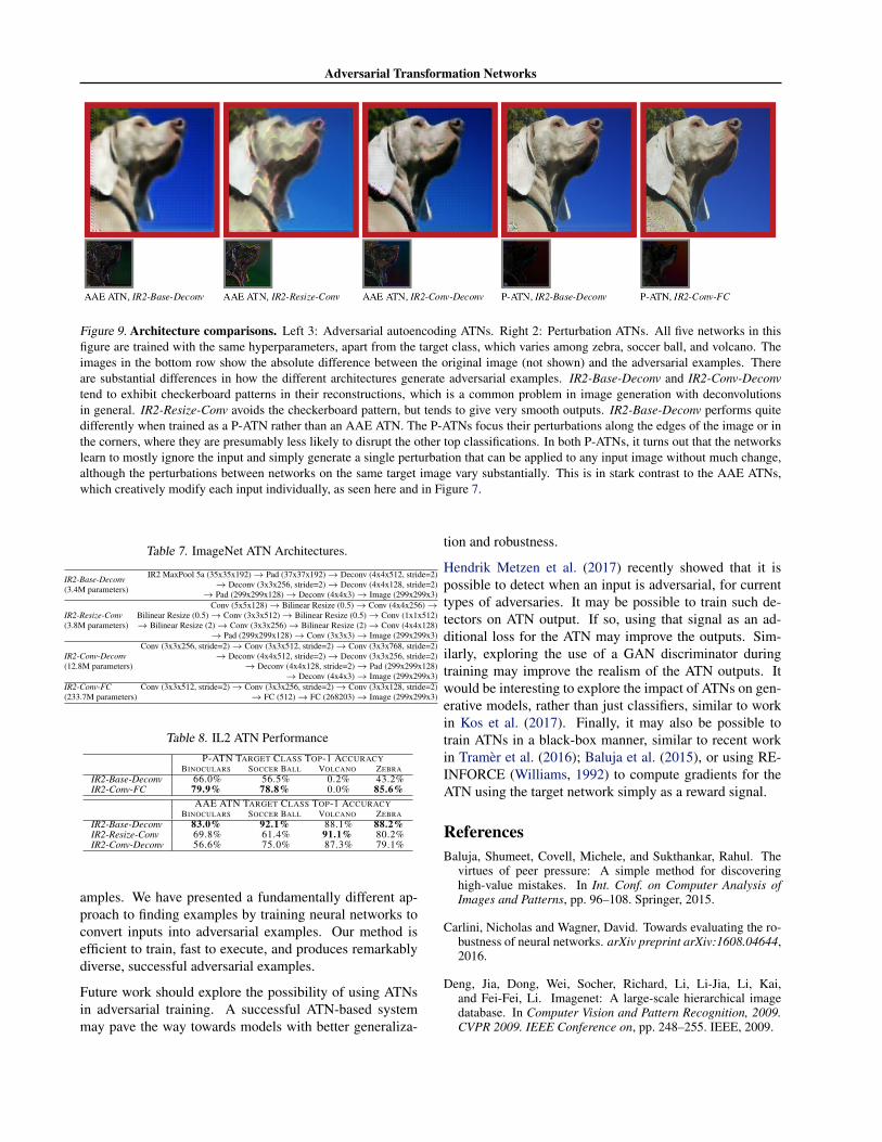
Figure 9. Architecture comparisons. Left 3: Adversarial autoencoding ATNs. Right 2: Perturbation ATNs. All five networks in thisfigure are trained with the same hyperparameters, apart from the target class, which varies among zebra, soccer ball, and volcano. Theimages in the bottom row show the absolute difference between the original image (not shown) and the adversarial examples. Thereare substantial differences in how the different architectures generate adversarial examples. IR2-Base-Deconv and IR2-Conv-Deconvtend to exhibit checkerboard patterns in their reconstructions, which is a common problem in image generation with deconvolutionsin general. IR2-Resize-Conv avoids the checkerboard pattern, but tends to give very smooth outputs. IR2-Base-Deconv performs quitedifferently when trained as a P-ATN rather than an AAE ATN. The P-ATNs focus their perturbations along the edges of the image or inthe corners, where they are presumably less likely to disrupt the other top classifications. In both P-ATNs, it turns out that the networkslearn to mostly ignore the input and simply generate a single perturbation that can be applied to any input image without much change,although the perturbations between networks on the same target image vary substantially. This is in stark contrast to the AAE ATNs,which creatively modify each input individually, as seen here and in Figure 7.

Table 7. ImageNet ATN Architectures.

IR2-Base-Deconv(3.4M parameters)

IR2 MaxPool 5a (35x35x192)→ Pad (37x37x192)→ Deconv (4x4x512, stride=2)→ Deconv (3x3x256, stride=2)→ Deconv (4x4x128, stride=2)

→ Pad (299x299x128)→ Deconv (4x4x3)→ Image (299x299x3)

IR2-Resize-Conv(3.8M parameters)

Conv (5x5x128)→ Bilinear Resize (0.5)→ Conv (4x4x256)→Bilinear Resize (0.5)→ Conv (3x3x512)→ Bilinear Resize (0.5)→ Conv (1x1x512)→ Bilinear Resize (2)→ Conv (3x3x256)→ Bilinear Resize (2)→ Conv (4x4x128)

→ Pad (299x299x128)→ Conv (3x3x3)→ Image (299x299x3)

IR2-Conv-Deconv(12.8M parameters)

Conv (3x3x256, stride=2)→ Conv (3x3x512, stride=2)→ Conv (3x3x768, stride=2)→ Deconv (4x4x512, stride=2)→ Deconv (3x3x256, stride=2)

→ Deconv (4x4x128, stride=2)→ Pad (299x299x128)→ Deconv (4x4x3)→ Image (299x299x3)

IR2-Conv-FC(233.7M parameters)

Conv (3x3x512, stride=2)→ Conv (3x3x256, stride=2)→ Conv (3x3x128, stride=2)→ FC (512)→ FC (268203)→ Image (299x299x3)

Table 8. IL2 ATN Performance

P-ATN TARGET CLASS TOP-1 ACCURACYBINOCULARS SOCCER BALL VOLCANO ZEBRA

IR2-Base-Deconv 66.0% 56.5% 0.2% 43.2%IR2-Conv-FC 79.9% 78.8% 0.0% 85.6%

AAE ATN TARGET CLASS TOP-1 ACCURACYBINOCULARS SOCCER BALL VOLCANO ZEBRA

IR2-Base-Deconv 83.0% 92.1% 88.1% 88.2%IR2-Resize-Conv 69.8% 61.4% 91.1% 80.2%IR2-Conv-Deconv 56.6% 75.0% 87.3% 79.1%

amples. We have presented a fundamentally different ap-proach to finding examples by training neural networks toconvert inputs into adversarial examples. Our method isefficient to train, fast to execute, and produces remarkablydiverse, successful adversarial examples.

Future work should explore the possibility of using ATNsin adversarial training. A successful ATN-based systemmay pave the way towards models with better generaliza-

tion and robustness.

Hendrik Metzen et al. (2017) recently showed that it ispossible to detect when an input is adversarial, for currenttypes of adversaries. It may be possible to train such de-tectors on ATN output. If so, using that signal as an ad-ditional loss for the ATN may improve the outputs. Sim-ilarly, exploring the use of a GAN discriminator duringtraining may improve the realism of the ATN outputs. Itwould be interesting to explore the impact of ATNs on gen-erative models, rather than just classifiers, similar to workin Kos et al. (2017). Finally, it may also be possible totrain ATNs in a black-box manner, similar to recent workin Tramer et al. (2016); Baluja et al. (2015), or using RE-INFORCE (Williams, 1992) to compute gradients for theATN using the target network simply as a reward signal.

ReferencesBaluja, Shumeet, Covell, Michele, and Sukthankar, Rahul. The

virtues of peer pressure: A simple method for discoveringhigh-value mistakes. In Int. Conf. on Computer Analysis ofImages and Patterns, pp. 96–108. Springer, 2015.

Carlini, Nicholas and Wagner, David. Towards evaluating the ro-bustness of neural networks. arXiv preprint arXiv:1608.04644,2016.

Deng, Jia, Dong, Wei, Socher, Richard, Li, Li-Jia, Li, Kai,and Fei-Fei, Li. Imagenet: A large-scale hierarchical imagedatabase. In Computer Vision and Pattern Recognition, 2009.CVPR 2009. IEEE Conference on, pp. 248–255. IEEE, 2009.


Gatys, Leon A., Ecker, Alexander S., and Bethge, Matthias. Aneural algorithm of artistic style. CoRR, abs/1508.06576, 2015.URL http://arxiv.org/abs/1508.06576.

Goodfellow, Ian, Pouget-Abadie, Jean, Mirza, Mehdi, Xu, Bing,Warde-Farley, David, Ozair, Sherjil, Courville, Aaron, andBengio, Yoshua. Generative adversarial nets. In Advancesin Neural Information Processing Systems, pp. 2672–2680,2014a.

Goodfellow, Ian J, Shlens, Jonathon, and Szegedy, Christian. Ex-plaining and harnessing adversarial examples. arXiv preprintarXiv:1412.6572, 2014b.

He, Kaiming, Zhang, Xiangyu, Ren, Shaoqing, and Sun,Jian. Deep residual learning for image recognition. CoRR,abs/1512.03385, 2015. URL http://arxiv.org/abs/1512.03385.

Hendrik Metzen, J., Genewein, T., Fischer, V., and Bischoff, B.On Detecting Adversarial Perturbations. ArXiv e-prints, Febru-ary 2017.

Johnson, Justin, Alahi, Alexandre, and Fei-Fei, Li. Perceptuallosses for real-time style transfer and super-resolution. In Eu-ropean Conference on Computer Vision, 2016.

Kingma, Diederik and Ba, Jimmy. Adam: A method for stochas-tic optimization. 2015.

Kos, Jernej, Fischer, Ian, and Song, Dawn. Adversarial examplesfor generative models. arXiv preprint arXiv:1702.06832, 2017.

Kurakin, Alexey, Goodfellow, Ian J., and Bengio, Samy. Adver-sarial examples in the physical world. CoRR, abs/1607.02533,2016a.

Kurakin, Alexey, Goodfellow, Ian J., and Bengio, Samy. Ad-versarial machine learning at scale. CoRR, abs/1611.01236,2016b.

LeCun, Yann, Cortes, Corinna, and Burges, Christopher JC. Themnist database of handwritten digits, 1998.

Linden, Alexander and Kindermann, J. Inversion of multilayernets. In Neural Networks, 1989. International Joint Confer-ence, pp. 425–430. IEEE, 1989.

Liu, Yanpei, Chen, Xinyun, Liu, Chang, and Song, Dawn. Delv-ing into transferable adversarial examples and black-box at-tacks. CoRR, abs/1611.02770, 2016. URL http://arxiv.org/abs/1611.02770.

Miyato, Takeru, Maeda, Shin-ichi, Koyama, Masanori, Nakae,Ken, and Ishii, Shin. Distributional smoothing with virtualadversarial training. In International Conference on LearningRepresentations, 2016.

Moosavi-Dezfooli, Seyed-Mohsen, Fawzi, Alhussein, Fawzi,Omar, and Frossard, Pascal. Universal adversarial perturba-tions. CoRR, abs/1610.08401, 2016a.

Moosavi-Dezfooli, Seyed-Mohsen, Fawzi, Alhussein, andFrossard, Pascal. Deepfool: a simple and accurate method tofool deep neural networks. In Proceedings of the IEEE CVPR,pp. 2574–2582, 2016b.

Mordvintsev, A., Olah, C., and Tyka, M. In-ceptionism: Going deeper into neural networks.http://googleresearch.blogspot.com/2015/06/inceptionism-going-deeper-into-neural.html, 2015.

Nguyen, Anh Mai, Yosinski, Jason, and Clune, Jeff. Deep neuralnetworks are easily fooled: High confidence predictions forunrecognizable images. CoRR, abs/1412.1897, 2014. URLhttp://arxiv.org/abs/1412.1897.

Odena, Augustus, Dumoulin, Vincent, and Olah, Chris. De-convolution and checkerboard artifacts. Distill, 2016.http://distill.pub/2016/deconv-checkerboard.

Papernot, Nicolas, McDaniel, Patrick, Jha, Somesh, Fredrikson,Matt, Celik, Z Berkay, and Swami, Ananthram. The limitationsof deep learning in adversarial settings. In Proceedings of the1st IEEE European Symposium on Security and Privacy, 2015.

Papernot, Nicolas, McDaniel, Patrick, and Goodfellow, Ian.Transferability in machine learning: from phenomena toblack-box attacks using adversarial samples. arXiv preprintarXiv:1605.07277, 2016a.

Papernot, Nicolas, McDaniel, Patrick, Goodfellow, Ian, Jha,Somesh, Celik, Z Berkay, and Swami, Ananthram. Practicalblack-box attacks against deep learning systems using adver-sarial examples. arXiv preprint arXiv:1602.02697, 2016b.

Szegedy, Christian, Zaremba, Wojciech, Sutskever, Ilya, Bruna,Joan, Erhan, Dumitru, Goodfellow, Ian, and Fergus, Rob.Intriguing properties of neural networks. arXiv preprintarXiv:1312.6199, 2013.

Szegedy, Christian, Ioffe, Sergey, Vanhoucke, Vincent, andAlemi, Alex. Inception-v4, inception-resnet and the im-pact of residual connections on learning. arXiv preprintarXiv:1602.07261, 2016.

Tramer, Florian, Zhang, Fan, Juels, Ari, Reiter, Michael K, andRistenpart, Thomas. Stealing machine learning models via pre-diction apis. In USENIX Security, 2016.

Ulyanov, Dmitry, Lebedev, Vadim, Vedaldi, Andrea, and Lempit-sky, Victor S. Texture networks: Feed-forward synthesis oftextures and stylized images. CoRR, abs/1603.03417, 2016.URL http://arxiv.org/abs/1603.03417.

Williams, Ronald J. Simple statistical gradient-following al-gorithms for connectionist reinforcement learning. Machinelearning, 8(3-4):229–256, 1992.

http://arxiv.org/abs/1508.06576







Documents

Adversarial Transformation Networks: Learning to Generate