Adverse Information and Mutual Fund Runs

Meijun Qian

A. Başak Tanyeri

National University of Singapore Bilkent University

August 2011

Abstract

This paper is the first one to document that anticipation of adverse events can trigger runs

in mutual funds. Using the event of the 2003 and 2004 litigations filed in the U.S. over

market-timing and late-trading practices, we find that runs start as early as six months

before litigation announcements. The pre-event runs are about half the size of runs that

follow announcements, which is about 1% of total assets per month. In addition, investors

who run before litigation announcements earn significantly higher risk- and peer-adjusted

returns than those who run after because, as the return data on fund holdings show, the

former avoid fire-sale costs. In funds holding illiquid assets or funds incurring large

outflows, the cumulative differences in abnormal returns can be as high as 6%. Hence,

our analysis suggests that a pro-rata ownership design is not sufficient to prevent runs in

mutual funds.

JEL: G23 G14

Keywords: Adverse event, mutual fund flows, runs, and returns

The authors would like to thank Edward Kane, Wayne Ferson, Phil Strahan, and Itay Goldstein for their

valuable comments. ** Department of Finance, NUS Business School. Tel: (65) 6516 8119; e-mail: bizqmj@nus.edu.sg

Faculty of Business Administration, Bilkent University. Tel: (90) 312-290-1871; e-mail: basak@bilkent.edu.tr

  2

1. Introduction

The first-come-first-served principle governing deposit withdrawals motivates

bank runs: every depositor wants to withdraw before others do because those at the back

of the line may not recover their deposits (Diamond and Dybvig, 1983; Chari and

Jagannathan, 1988). In contrast, mutual funds allocate the proceeds from asset sales on a

pro-rata basis, a design that should shield mutual funds from runs. Mutual funds,

however, may prove susceptible to runs on revelation of adverse information about the

quality of management or underlying assets, even though a physical queue of

withdrawers, as in bank runs, is absent. This paper provides direct evidence of pre- and

post-event runs in the mutual fund industry and the reasons such runs may take place.

We define a fund run as an abnormally concerted redemption of mutual fund

shares in anticipation or revelation of an adverse event. The adverse events we focus on

are the 2003 and 2004 litigations in the U.S. alleging that certain mutual funds allowed

some investors to engage in late trading and market timing,1 thereby allowing them to

enjoy profits at the expense of investors who did not engage in these practices. Upon the

suspicion or revelation that fund managers do not serve the interests of all investors

equally, disadvantaged investors may discipline the implicated funds by withdrawing

existing investments and/or by withholding new investments.

We first document the pre- and post-event runs around litigation announcements.

We find not only that fund runs occur both prior to and post litigation announcement, but

1 Late trading is the purchase or sale of mutual fund shares after determination of the net asset value (NAV) at 4:00 PM. Market timing is the short-term trading of mutual fund shares to exploit price inefficiencies between the mutual fund shares and underlying securities in the funds’ portfolios. A representative case of such practices is detailed in the Bank of America Nations Fund Securities Litigation Complaint available at http://securities.stanford.edu/1028/BAC03-01/20030905_f01c_Lin.htm.

  3

also that pre-event runs start as early as six months before such announcements. During

these six months, flows to implicated funds are 2.28% lower than flows to non-implicated

funds and remain lower for at least two years post event. The abnormal outflows from the

implicated funds average about 1.42% of TNA per month in the six months following

litigations.

We also investigate the motivations for runs other than disciplining management;

in particular, the benefits of redeeming shares before the adverse information becomes

public (i.e., pre-event runs). The rationale for this focus is as follows. Concerted

redemption and the lack of new sales that follow litigation announcements force funds to

liquidate assets quickly, and, as Coval and Stafford (2007) show, a large selling volume

by institutional investors temporarily depresses underlying asset prices. Because

shareholders who redeem shares at this time will suffer losses, investors who can

anticipate litigations and the subsequent redemption congestion have incentives to

redeem shares before the litigation announcements. By exiting early, informed investors

avoid the fire-sale costs caused by subsequent concerted withdrawals. The empirical

evidence confirms these hypotheses. We find that investors who run before litigation

announcements earn significantly higher risk- and peer-adjusted returns than those who

run after. In funds holding illiquid assets, this difference can be as high as 6%

accumulated from six months prior to six months post litigation.

To argue that the return difference itself motivates, and thus amplifies, the fund

runs in addition to penalizing management, however, we must examine the cross-

sectional differences in fund vulnerability to run and the difference-in-difference of

returns for pre- and post-event withdrawals in litigation events with quite homogenous

  4

legal severity. The incentive for early runs will be greater for funds whose return

differences due to withdrawal timing are larger either because they hold illiquid assets or

because they are likely to suffer larger outflows upon the announcements. Consistent

with this implication, we find that funds holding illiquid assets or who are expected to

suffer large outflows (e.g., funds with a history of Securities and Exchange Commission

(SEC) investigations) experience more severe runs both prior to and post litigation

announcements. The return difference between investors who run before litigation

announcements and those who run after is also more pronounced for these types of funds

than for their counterparts. Finally, we verify the implicit assumption of the argument by

showing empirically that the return difference between early and late redemptions is

indeed driven by fire-sale costs: the event returns of firms held by implicated funds are

negative and significant.

Our results thus indicate that mutual fund investors who anticipate negative flows

motivated by such adverse events as litigation have incentives to withdraw early and

avoid fire-sale costs. The existence of motivation for early withdrawal has an important

implication for fund industry stability. When the timing of the action (runs) matters for

payoff (returns), strategic complementarities come into play that can amplify the impact

of adverse events on fundamentals and generate financial fragility. Nonetheless, mutual

fund runs may not occur unless there is a systematic liquidity shock to all fund investors,

like those assumed in Chen et al. (2010)’s model. In the absence of such a shock, other

  5

investors will purchase the assets at fire-sale prices and may thus correct the mispricing

(Chen et al., 2008).2

This financial fragility of the mutual fund industry is underscored by the U.S.

Treasury’s decision to insure the holdings of eligible money-market mutual funds in the

wake of the turmoil caused by the run on the Reserve Primary Fund in September 2008.3

Our findings explain exactly why the demise of Lehman Brothers can lead to such

fragility. The Reserve Primary Fund held debt securities from Lehman Brothers, whose

redemption following the Lehman Brothers bankruptcy totaled about two-thirds of its

total net assets (Wall Street Journal, 2008; New York Times, 2008). Because of the

simultaneous liquidity crunch in the short-term credit market, to satisfy such

redemptions, non-redeeming investors would have had to bear the fire-sale costs

associated with asset sales.

As the first academic paper that documents an actual mutual fund run and

numerates incentive for mutual fund runs in anticipating of adverse information, our

paper therefore makes an important contribution to the mutual fund run literature, which

at present consists of only few papers. Among these (and most likely the only one), Chen

et al. (2010), using a global capital allocation model, theoretically argue that strategic

complementarities exist in mutual funds because of the costs that withdrawals impose on

investors who stay with the funds. The empirical evidence in their paper, however, limits

2 Chen et al. (2010) show that hedge funds that purchase funds’ underlying assets at the depressed price during fire-sale periods generate arbitrage profits similar to the profits of the short sellers. However, short selling is not allowed in most mutual funds. 3 The Treasury thus expressed its concerns about the ensuing uncertainty in the mutual fund industry and justified its instatement of a guarantee program as follows: “…Maintaining confidence in the money market fund industry is critical to protecting the integrity and stability of the global financial system. …This action should enhance market confidence and alleviate investors' concerns about the ability for money market mutual funds to absorb a loss…” (U.S. Treasury Department press release, 19 September, 2008).

  6

to an indirect test of the model by showing the cross-sectional differences in the fund

flow performance relation. Our paper not only provides direct evidence of fund runs but

also, by focusing on an unambiguously important event in which withdrawals were a

major issue for the industry, analyzes the return differences resulting from fire-sale costs

for concerted outflows to investors withdrawing pre and post event. These return

differences between differently timed withdrawals give the most direct evidence for why

strategic complementarity may also play a role in mutual funds.

The rest of the paper proceeds as follows: Section 2 develops the methodology,

Section 3 describes the data, Section 4 outlines the empirical results, and Section 5

concludes the discussion.

2. Research method

The argument developed in the introduction can be formulated into four specific

empirical problems: whether informed investors run implicated funds prior to and post

litigation announcements, whether investors who run funds prior to litigations realize

higher returns than those who run post, whether some types of funds are more susceptible

to pre-event runs, and whether the low returns on post-litigation withdrawals are indeed

caused by fire-sale costs.

2.1. Detecting pre-event runs

To document pre-event runs, we need benchmarks of normal flow, the first of

which are flows to peers not named in the 2003 and 2004 lawsuits. For this benchmark,

we construct three groups of funds: funds whose management companies are not

involved in these litigations (funds in non-implicated families), funds not named in the

suits but whose management companies are named (non-implicated funds in implicated

  7

families), and funds named in the suits (implicated funds). We then compute the fund

flows as follows:

Flowi,t = [TNAi,t –TNAi,t-1 *(1+ri,t)] / TNAi,t-1, (1)

where Flowi,t is net flows of fund i in month t, TNAi,t-1 and TNAi,t are total net assets of

fund i in month t-1and t, respectively, and ri,t is the return of fund i in month t. To detect

whether implicated funds have lower flows than non-implicated funds, we compare the

net flows of the three groups around the litigation dates.

The second benchmark for normal flows is the estimated net flows from a model

designed to capture the main determinants of fund flows. Because past returns predict

future flows (Gruber, 1996; Chevalier and Ellison, 1997; Sirri and Tufano, 1998; Zheng,

2000; Del Guercio and Tkac, 2001, 2002) and industry-level and style-level flows explain

individual fund-level flows (Qian, 2011), we develop a model that includes variables for

fund characteristics, past returns, and industry- and style-level flows. To detect pre-

litigation and post-litigation runs, we also construct 25 event-window indicators, to

produce the following model:

Flowi,t = a + ∑bj * fund characteristicsi,t j + ∑cj * past returnsi

j

+ ∑dj * aggregate flowst j + ∑γj * Event-window indicatorsi,t

j +εi,t, (2)

where fund characteristics are size, the log of TNA; age, the log of days since the first

offer date; 12b-1 fees, the annual fees paid to financial advisors, measured as a

percentage of TNA; and front and rear loads, the charges for share purchase and

redemption as a percentage of TNA. Past returns include compounded returns in the past

one (Ri,t-1), three (∏s(1+ Ri,t-s)-1, s=1, 2,3), and six months (∏s(1+ Ri,t-s)-1, s=1,2,---,6).

Aggregate flows include both industry- and style-level flows: industry-level flows are the

  8

sum of flows in dollars (Σi (TNAi,t –TNAi,t-1*(1+Ri,t ))) to all funds in the sample divided

by the sum of the lagged TNA (Σi (TNAi,t-1)), and style-level flows are the sum of flows in

dollars to all funds with the same investment style divided by the sum of the lagged TNA.

We adopt the style classification of Pastor and Stambaugh (2002) and Ferson and Qian

(2005), which contains the following eight categories: aggressive growth, growth-

income, global equity, other equity, bond funds, municipal funds, money market, and

other. The event-window indicator (n month) equals 1 if it is the nth month from the date

of the litigation filing and 0 otherwise (n = -1, -2…12, 0, 1, 2…12).

2.2 Rationale for pre-event runs

Despite that proceeds from asset sales are determined by the prices of underlying

assets and distributed pro-rata, shareholders may still have the following incentives to run

a mutual fund: Because abusive behaviors indicate how faithfully fund managers serve

investors’ best interests fairly, investors may want to redeem shares as soon as they are

informed, publicly or privately, that the funds invested in are engaging in abusive

practices like market timing or late trading. If and when a sufficient number of investors

learn of a fund’s abusive behavior, a run may ensue. Consequently, because mutual funds

must liquidate assets quickly to satisfy share redemption, if large selling volumes

temporarily depress underlying asset prices, shareholders who redeem shares at this point

will realize negative abnormal returns.

We examine whether investors who withdraw prior to the revelation of abusive

behavior avoid costs using two approaches, the first of which benchmarks normal returns

using five portfolio return models and introduces indicators for pre- and post-event

months to identify return differences between investors who withdraw pre- and post-

  9

litigations. These five return models are the market model (Sharpe, 1964; Lintner, 1965),

the market model with lagged market returns (Scholes and William, 1977), the Fama-

French benchmark model (Fama and French, 1992, 1993), the Fama-French benchmark

model with a fourth factor that captures momentum (Jegadeesh and Titman, 1993;

Carhart, 1997), and the market model with a factor that captures liquidity (Pastor and

Stambaugh, 2003):

ri,t = α + β*r m.t + ∑αn * Indicatorn+ ε i,t, (3)

ri,t = α + β1*r m.t + β2*rm.t-1 + ∑αn * Indicatortn + ε i,t , (4)

ri,t = α + ∑βj * FFtj + ∑αn * Indicatort

n+ ε i,t, (5)

ri,t = α + ∑βj * FFtj + γ1* MOMt + ∑αn * Indicatort

n + ε i,t, (6)

ri,t = α + β*rm.t + γ2*LIQt+ ∑αn * Indicatortn + ε i,t . (7)

where ri,t is the excess returns (net of the risk-free rate) of fund i for month t, and rm.t is

the excess market return for month t. FFj includes market returns, size (SMB), and value

(HML) factors; MOM is the momentum factor; and LIQ is the liquidity factor. The event-

window indicator (n month) equals 1 if it is the nth month from the date of the litigation

filing and 0 otherwise (n = -1, -2…-6, 0, 1, 2…6).

2.3. Impact of fund characteristics and liquidity on pre-event runs

Pre-event runs are motivated by suspicions of litigation and anticipation of the

liquidation costs that would arise to satisfy post-litigation redemption. Hence, investor

decisions to run before confirmation of the adverse event are influenced by their beliefs

about or awareness of abusive behavior and by factors that would increase fire-sale costs.

The likelihood that investors become suspicious of funds’ abusive behavior may in turn

be affected by the fund management’s reputation and the investors’ ability to collect and

  10

process information. We measure fund reputation using ownership structure and a history

of SEC charges; that is, investors may judge funds in conglomerate families as less likely

to engage in abusive behavior because loss of reputation would hurt both the abused fund

and the other businesses in the conglomerate. Hence, the consequences of abusive

behavior may be larger for conglomerates than for fund families that only focus on

managing mutual funds. Likewise, past actions may predict future decisions; for example,

investors may judge funds with no history of abusive behavior as less likely to engage in

abusive behavior in the future. We measure investors’ information collection and

processing ability based on their types. More specifically, large institutional investors can

be expected to more readily anticipate abusive behavior and possibly redeem shares in

implicated funds prior to lawsuit filing.

To investigate whether fund and investor characteristics influence the

susceptibility of funds to pre-event runs, we generate dummy variables for five

characteristics: conglomerate, charge history, large institution, fund, and investor

characteristics. The first three indicators equal 1 if the fund is part of a conglomerate, has

undergone an SEC investigation in the past eight years, and caters to large institutional

investors only; 0 otherwise. We interact the dummy variables for fund and investor

characteristics with all the variables in Equation (2).

The economic rationale for pre-event runs is the liquidation cost (price

depression) that funds bear when they are forced to sell assets upon revelation of an

adverse event. This liquidity cost increases with the illiquidity of underlying assets and

with the volume of redemptions. Hence, investors in funds with illiquid assets, such as

real estate investment trusts (REITs), international assets, or municipal funds, have

  11

stronger incentives to run because the benefits may be greater. We therefore investigate

the impact of underlying asset liquidity on run incentives and investor benefits from

running early by generating a dummy variable (liquid) for liquid funds. We then

categorize funds as liquid or illiquid based on the assets they invest in as defined in the

style classification. Whereas liquid funds invest in large-cap stock and treasury bills,

illiquid funds invest in small-cap stocks, sector stocks, international equity and bonds,

and asset-backed securities. Finally, we interact the liquid dummy with all the variables

in Equations (3)–(7).

We conduct these analyses using a two-step fund-by-fund approach and then a

panel approach, which, although its pooling of information from all funds is efficient,

may suffer from the problem that all fund coefficients must be the same. In the fund-by-

fund estimation, the first step estimates the flow model and the five return models for

each fund using time-series observations only. The control variables for the flow analysis

include accumulated returns in the past one, three, and six months, as well as industry-

and style-level flows. The explanatory variables include two indicators whose

coefficients estimate the pre-event runs and runs (from the flow-model estimation), as

well as the risk-adjusted returns (from the returns-models estimation) six months pre and

post event. The second step compares the estimated silent runs and the risk-adjusted

returns in cross section. We investigate differences by fund groupings based on SEC

charge history, ownership structure, investor clienteles, liquidity of underlying assets, and

the magnitude of outflows in the post-event window.

2.4 Cost of fire sales

  12

A direct test of whether mutual funds bear the costs associated with liquidating

portfolio positions is to analyze the returns to underlying stocks in fund portfolios. To do

so, we compile the holdings of implicated and non-implicated funds in every week of

September 2003 and then calculate the abnormal returns to the shares held by both types

of funds. We choose September 2003 as the month in which the trades of implicated

funds most reflect the withdrawals associated with litigation and calculate abnormal

returns to stocks held by implicated and non-implicated funds.

To compute the cumulative abnormal returns (CARs), we estimate the market

model—which uses the CRSP equally weighted portfolio as the market portfolio—for

each firm using daily returns from 282 days to 30 days prior to the litigation

announcements. We then aggregate the weekly CARs using estimated daily abnormal

returns for the weeks of September 2–4, September 7–11, September 14–18, and

September 21–25 of 2003.

3. Data

To identify the funds and fund families implicated in the market-timing and late-

trading litigations, we conduct a keyword search of the Financial Times4 and the Wall

Street Journal. We also search the SEC litigation filings on the EDGAR and in the

Stanford Law School Securities Class Action Clearinghouse.5 Table 1 summarizes the

results of this search, including the names of the implicated fund families, the activities

for which they were indicted, the regulatory authorities involved, the litigation

4We use three keywords---investigation, mutual fund, and Spitzer---to search the Financial Times and Wall

Street Journal between September 3, 2003, and December 31, 2005. 5

Stanford Law School Securities Class Action Clearinghouse (available online at http://securities.stanford.edu/index.html) compiles detailed information on the prosecution, defense, and settlement of federal class-action securities fraud litigations.

  13

announcement dates, and the names of the parent companies. We also use the Stanford

clearinghouse database to identify funds within each implicated fund family explicitly

named in the litigation.

The formal investigation into the trading practices of mutual fund companies

began on September 3, 2003, when New York Attorney General Eliot Spitzer filed a

complaint in the New York Supreme Court alleging that the mutual fund companies of

Bank of America Corp., Bank One Corp., Janus Capital Group Inc., and Strong Capital

Management Inc. had allowed certain hedge fund managers to trade illegally in their fund

units. Subsequently, between September 2003 and August 2004, the SEC, the New York

State Attorney General, and other regulatory authorities filed litigations involving funds

in 25 mutual fund families.

Although the formal announcement of the first litigation came on September 3,

2003, the first news article revealing the ongoing investigation is dated September 1,

2003, and other news articles on abusive trading practices by mutual funds even predate

September 2003. In fact, the SEC was aware of the fair pricing problems in mutual funds

as far back as 1997, and the probe into hedge fund trades that take advantage of such

problems had been underway since 2002. The first article indicating the possible active

involvement of mutual fund management is dated March 5, 2003, and by March 26,

2003, Congress had begun talking about strengthening mutual fund regulation. It is

highly probable, therefore, that investors had begun to suspect abusive behavior and

potential investigations by March 2003. We thus expect the pre-event indicators in our

models to capture whether investors did indeed suspect abusive behavior and take

corresponding action as early as this date.

  14

For the universe of mutual funds, we rely on the CRSP mutual funds database

(from WRDS), which provides monthly observations of funds’ total net assets (TNA) and

returns (R). We merge our own list of implicated funds with the CRSP universe of funds

using ticker symbols to produce a sample in which implicated funds are differentiated

from non-implicated funds. We exclude all funds with missing ticker symbols, funds in

their incubation period, funds having fewer than 12 months of observations, and funds

whose TNA is smaller than 5 million USD. Because we observe outliers in the flows

(e.g., negative flows that are larger than the TNA and positive flows that are five times

larger than the TNA), we windsorize the sample at the first and 99th percentiles to reduce

the outlier effect. The final sample contains 8,703 funds, of which 1,102 are implicated

funds and 1,003 are non-implicated funds in implicated families. The observation unit is

the fund month, and there are 763,072 fund months from February 1996 to December

2005.

Panels A and B of Table 2 provide a profile of the funds in non-implicated

families, and the implicated and non-implicated funds in implicated families as of

December 2002 and December 2004, respectively. Specifically, the panels show the

number of funds, the mean, and the total TNA of funds in each group. In terms of this

latter, funds in the sample were managing 4.7 trillion USD as of December 2002 and 5.5

trillion USD as of December 2004. In December 2002 and 2004, 65% and 62% of total

funds under management, respectively, were controlled by implicated families, with the

average implicated fund being larger than the average non-implicated fund.

Although the WRDS database provides information on fund characteristics like

expense structure (12b-1 fees, rear and front loads), investment style, age (age), and

  15

investor type (retail and institutional funds), we identify the funds of large institutions

using MorningStar’s data on funds’ intial buy restriction. We also hand collect data on

certain fund characteristics; for example, we use SEC EDGAR filings and firm websites

to determine whether the parent company is a conglomerate or an asset management

company, and SEC litigation filings to check whether funds have a prior history of SEC

charges. To estimate fund performance, we compile monthly data on market returns (rm);

risk-free rate (rf); and value (SMB), size (HML), momentum (MOM), and liquidity (LIQ)

factors using WRDS’s Fama-French, momentum, and liquidity databases; and draw

information on mutual funds’ quarterly portfolio holdings from its 13-F Institutional

Holdings database. Finally, we compile daily stock and market returns for computing

abnormal returns around the event days from CRSP.

4. Empirical Results

We arrange our findings around the four empirical questions. First, we investigate

whether investors run implicated funds both prior to and post litigation announcements

and determine whether the size of pre-event runs is statistically and economically

significant. Second, we examine whether investors who run prior to litigation

announcements earn higher risk-adjusted returns than do investors who run post

announcements. Third, we analyze how fund and investor characteristics and liquidity of

underlying assets may affect the timing and size of runs and the costs to investors who

run after the public announcement of litigation, or in a relative sense, the benefits that

investors can reap from running early versus late. Finally, using fund holding and stock

return data, we empirically assess whether the cost of running late does indeed come

from fire-sale costs.

  16

4.1 Detecting pre-event runs

We detect pre-event runs using two benchmarks: a univariate analysis to

benchmark the flows of implicated funds against the flows of funds in non-implicated

families, and a multivariate analysis to benchmark the flows of implicated funds against

the flows estimated using the normal-flow model. The average monthly flows of funds in

non-implicated families, non-implicated funds in implicated families, and implicated

funds from September 2001 to September 2005 are plotted in Figure 1, in which the

straight line indicates the month of the first litigation filing (September 2003). As the

figure shows, before April 2003, the flows of implicated funds are either higher than or

no different from the flows of funds in non-implicated families, but after this date, they

are consistently lower. That is, a shift occurred four months before the first litigation

filing, suggesting that investors ran funds both before and after the announcement of the

first litigation.

The results in Table 3 confirm that the trends in Figure 1 are statistically

significant. In the months prior to September 2003, the flows to implicated funds are

statistically larger than the flows to funds in non-implicated families, especially from

September 1 to August 2002. However, this trend reverses in the four months prior to

September 2003. Likewise, implicated funds that enjoyed large flows up to one year

before the onset of litigation begin to experience runs before September 2003 and

continue to do so for the two years after September 2003 (numbers in the first year are

given in Table 3). The flows of non-implicated funds in implicated families are also

significantly lower than the flows of funds in non-implicated families. These results

suggest that investors may see involvement in lawsuits as an indicator of fund family

  17

managers’ failure to serve investor interests. As a result, they punish all funds in

implicated families regardless of whether the fund in question allowed abusive practices

or not (a spill-over effect).

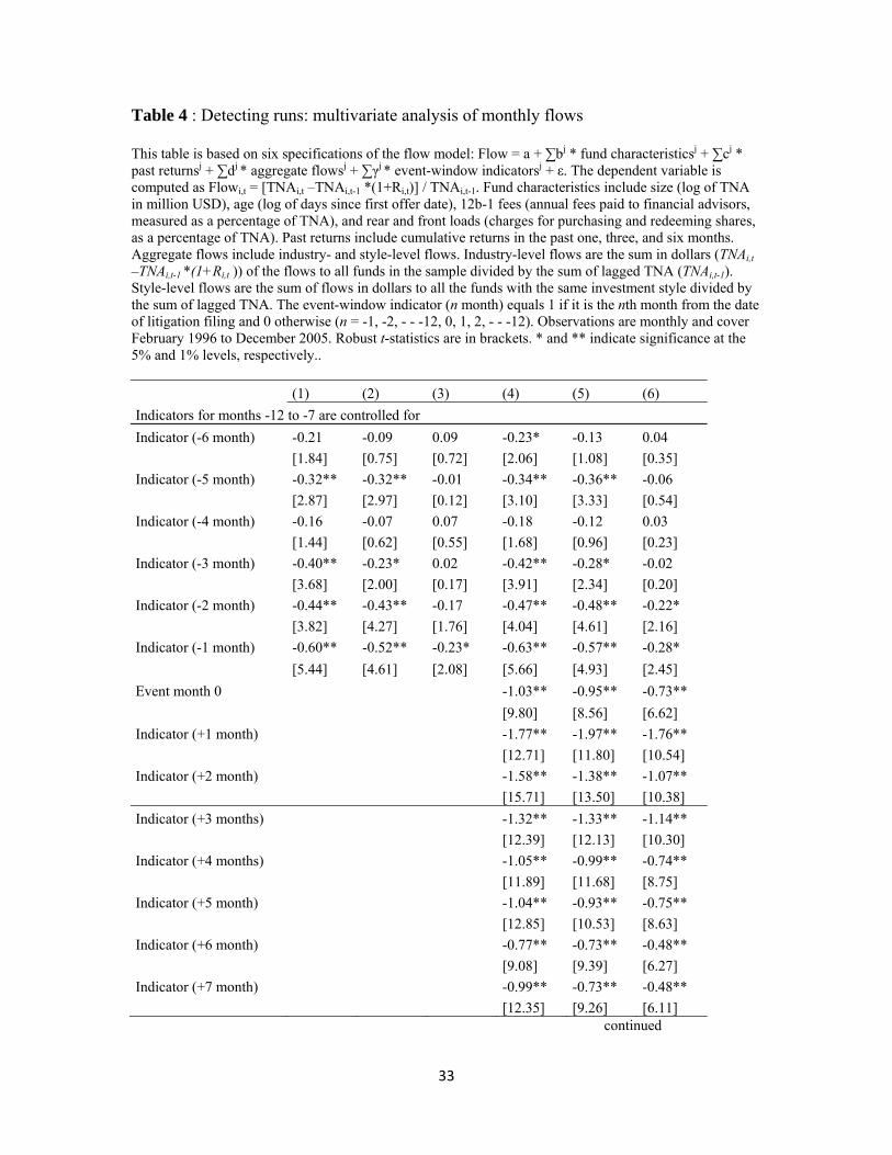
Table 4 provides estimations of the flows model described in Equation (2), which

assesses whether implicated funds realize abnormal flows around litigation dates. Here,

monthly flows are regressed on four sets of controls—fund characteristics, past returns,

fee structures, and aggregate flows—and on indicator variables for event-window months

that extend 12 months before and after litigation announcements.6 Table 4 thus includes

six specifications: one that controls for fund characteristics and historic returns; a second

and third that introduce controls for fee structure and flow characteristics, respectively;

and three that introduce post-announcement indicators into the first three specifications.

The observation unit is monthly flows from February 1996 to December 2005, and the

regressions use cluster-robust variance/covariance estimators in which the clusters are

funds.

The results in Table 4 confirm the presence of the runs (pre-event and otherwise)

previously indicated in Figure 1 and Table 3. The table shows a significant outflow in

implicated funds starting as early as six months prior to litigation announcements in the

fourth specification and as late as one month in the third specifications. These significant

outflows continue during the 12 months following litigation announcements. The size of

the runs ranges from -23 to -63 basis points in the month prior to the litigation

announcements and from -176 to -197 basis points afterwards. Such significant outflows

6 We estimate Equation (2) using fund fixed effects. The results are available upon request and remain

qualitatively the same.

  18

indicate that investors run implicated funds as soon as they suspect oncoming litigations

in the case of pre-litigation outflows and as soon as litigations are filed in the case of

post-litigation outflows.

These four sets of controls produce significant results. First, younger and larger

firms enjoy significantly higher flows than do their older and smaller counterparts.

Second, investors chase past returns. Third, funds with high transaction costs (as

measured in loads) and fees (as measured in 12b-1 fees) realize lower flows. Fourth,

industry-level and style-level flows matter. When the industry or style is enjoying larger

flows, so do the individual funds.

4.2 Costs associated with running early versus late

We also investigate whether benefits exist for investors who run implicated funds

prior to litigation announcements. Pooling all available data on implicated and non-

implicated funds, we estimate models of normal returns to identify the return differences

to implicated funds in the months surrounding litigation announcements.7 Monthly

returns from January 2000 to December 2005 are regressed on risk factors and indicator

variables for event-window months as described in Equations (3) through (7).8 To detect

return differences, we also test for differences in the coefficients of the event-window

indicators. Here, all regressions use cluster-robust variance-covariance estimators in

which the clusters are mutual funds.

7 We employ an alternative approach to detect return differences. We first estimate Equations (3) through

(7) for each implicated fund separately and then test whether the coefficients of pre- and post-event months differ. We find that the differences in coefficients are significant in the market model but insignificant in the other models. 8

We estimate Equations (3) through (7) using fund fixed effects. The results are available upon request and remain qualitatively the same.

  19

As Panel A of Table 5 shows, investors who run implicated funds after litigation

announcements put up with low returns. Indeed, the estimates from the market model

indicate that the cost of exiting implicated funds in the six months following litigation

announcements range from no cost in the fifth month to 40 basis points in the second

month. In contrast, investors benefit from exiting implicated funds in three out of the six

months preceding litigation announcements. The results of the other four returns models

are qualitatively similar.

Our results clearly indicate that, consistent with Coval and Stafford’s (2007)

argument that prices of underlying assets become depressed when there is a large volume

of asset sales, investors who exit implicated funds before other investors do indeed avoid

the lower returns suffered by those who exit after litigation announcements. As Table 4

shows, mutual funds face large outflows following litigation announcement and may thus

suffer fire-sale costs when they try to liquidate their portfolios to satisfy the high

redemption volume. These fire-sale costs would explain the lower returns observed

following litigation announcements.

Panel B of Table 5 shows our assessment of whether investors benefit from

exiting implicated funds prior to litigation announcements. Specifically, in the first rows

of the five event windows (which range from one to five months), we list the differences

between the accumulated coefficients of event-month indicators before and after

litigation announcements. In the second rows, we report the F-statistics for the test in

which the difference is equal to 0. For the one-month window, the difference in

coefficients pre- and post- announcement ranges from 58 basis points to 64 basis points.

For the three-month window, the difference in accumulated coefficients pre- and post-

  20

announcement ranges from 65 basis points to 112 basis points. These differences are both

economically and statistically significant.

This evidence for pre-event runs and return differences between pre- and post-

event runs suggests that the timing of redemption matters for returns despite the pro-rata

distribution of proceeds from asset sales in mutual funds, and that, if investors are to

penalize management, it is rational for them to do so before the adverse information

becomes public.

4.3 Cross-sectional difference in runs and returns

We also conduct fund-by-fund estimations of the cross-sectional differences in

fund runs and returns before and after litigation announcements. Specifically, we add two

indicators into the flow and returns models (Equations 2 to 7)—one for the six-month

pre-event window and the other for the six-month post-event window—and estimate

fund-by-fund the pre- and post-event runs and returns. We then summarize these fund-

level estimates and compare them across different fund groups. The results are given in

Table 6.

Panel A of Table 6 summarizes the coefficients estimates on the indicators of the

six-month pre- and post-event runs, with the cross-sectional mean and t-statistics of the

runs for all implicated funds listed in column 1. As the column shows, not only are the

abnormal flows in both event windows significantly negative, which implies the

existence of fund runs both before and after litigations, but post-event runs are larger than

pre-event runs (-1.44% vs. -0.42%). The remaining columns present the differences in pre

and post runs across groups. Funds without an SEC charge history experience

significantly smaller pre-event runs than those with a charge history. Likewise, funds that

  21

belong to financial conglomerates experience significantly fewer runs both before and

after litigations. Finally, post-event runs are significantly larger for funds with illiquid

assets than for those with liquid assets. These results are consistent with our hypothesis

on the effects of reputation and liquidity on fund runs.

In addition, as panel A of Table 6 shows, post-event runs are much smaller in

large institutional funds than in retail funds. This finding is consistent with the argument

put forward by James and Karceski (2006) that large institutions are more sophisticated

monitors than retail investors and small institutions. Most particularly, they understand

that share value is determined by the underlying assets, meaning that selling shares at the

time of the fund’s fire sale would impose losses.

Panel B of Table 6 provides a comparison of the coefficient estimates on the six

months pre- and post-event indicators from the returns models; that is, the estimates of

the return benefits of pre-event runs relative to those of post-event runs. The first column

presents the return benefits for all implicated funds, while the remaining columns list the

average return differences and t-statistics across groups. As is apparent, the risk-adjusted

returns (alpha) are significantly higher in the pre-event window than in the post-event

window, especially for retails funds, funds with illiquid assets, and funds with large post-

event outflows. These results are consistent with our hypothesis that liquidity and the

magnitude of runs affect the fire-sale costs associated with redemptions.

Not only can liquidity of underlying assets affect runs and return differences, so

can fund reputation. In fact, fund reputation can also alleviate investors’ suspicion of

mismanagement and reduce runs, which in turn may decrease the probability of financial

contagion. In Table 7, therefore, we report the results of our panel approach, an

  22

augmented version of the flow model given in Equation (2), which is designed to

determine whether fund reputation affects investor decisions to run and thus fund

susceptibility. This augmented model interacts the dummy variables for fund

characteristics with every term in the original equation. The first two columns in the table

list the management’s ownership type and the last two columns, its SEC charge record.

Both sets of regressions use cluster-robust variance-covariance estimators in which the

clusters are funds, and each regression generates two sets of coefficients, one for stand-

alone variables and the other for interaction terms.

The estimations clearly show that runs on implicated funds with conglomerate

parents are less significant both prior to and post litigation filing, which implies that

investors are less suspicious of abusive behavior by conglomerate-operated funds and

punish them less even when abusive behavior is revealed. In fact, the absence of pre-

litigation runs suggests that conglomerates may be perceived as more reputable and hence

less likely to engage in abusive trading practices. However, the absence of post-litigation

runs may indicate that investors do not run conglomerates for abusive practices and/or

they believe conglomerates to be better equipped to deal with the aftermath and financial

consequences of litigation.

The results given in columns 5 and 6 of Table 7 also indicate that SEC charge

history affects the timing of runs but not their size. That is, prior to litigations, investors

are less suspicious of abusive practices in funds with no history of SEC investigations.

Reputation is lost, however, as soon as investors learn of abusive practices. Hence, even

though in the eyes of the law, fund managements may be innocent until proven guilty,

investors apparently presume guilt as soon as they learn of litigation.

  23

Finally, we examine the effect of underlying asset liquidity on the return

difference between withdrawals made prior to and post announcements. Because the

benefit of pre-event runs is avoidance of the liquidation costs (price depression) borne by

investors when revelation of an adverse event forces funds to sell assets, investors in

funds with illiquid assets (e.g., REITs, international assets, or municipal funds) have

stronger incentives to run because of potentially greater benefit.

To assess this effect, we apply a panel approach to the augmented version of the

returns model described in Equations (3) through (7), which interacts the liquid fund

indicator with every term in the equations. Here, monthly returns from January 2000 to

December 2005 are regressed on indicator variables for the event-window months, the

risk factors, and the interaction terms, although we omit the coefficients on the stand-

alone variables and interaction terms to avoid excessively long tables. The results

indicate that investors in liquid funds enjoy higher returns than investors in illiquid funds

during the four months surrounding litigation announcements. In all specifications of the

returns model, returns to illiquid funds are negative up to three months prior to litigation

announcement and remain negative up to four months afterwards.

We therefore test for differences in the accumulated coefficients of event-window

indicators and their interactions with the liquid indicator. As shown in Table 8, Panel A,

in all specifications and event-windows, there are significant differences in returns

between investors in illiquid funds who exit before the announcement and those who do

so after it. As Panel B shows, however, the return differences between investors in liquid

funds who exit pre and post announcement are less pronounced. These results therefore

support the hypothesis that liquidation cost is higher in illiquid funds.

  24

In sum, consistent with the argument on penalizing mismanagement and fire-sale

costs, pre-event runs are more prominent in funds with bad reputations and illiquid assets.

That is, because investors are more likely to suspect irreputable funds, redemptions from

such funds on public announcement of trading mispractices are larger. Likewise, because

funds that invest in illiquid assets are more likely to suffer from fire-sale costs when they

try to satisfy redemptions, the return differences before and after litigations are greater.

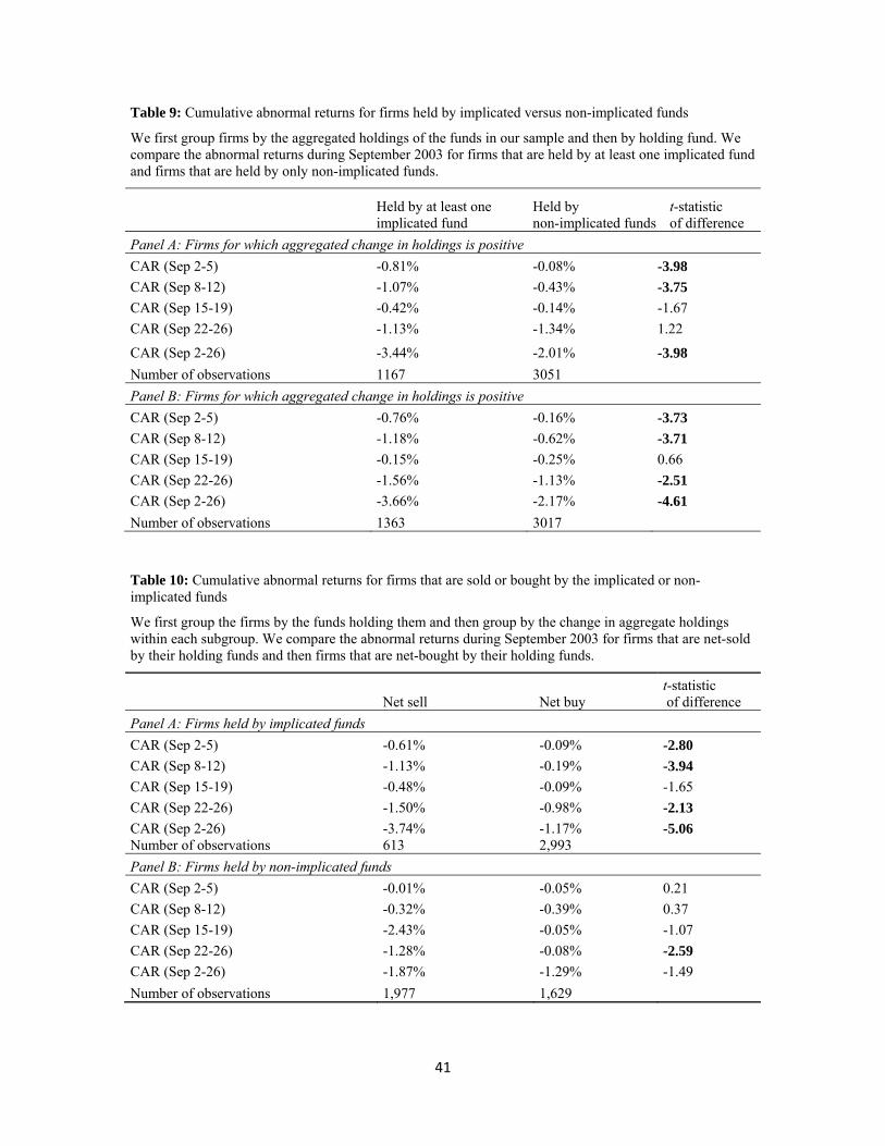
4.4 Evidence from holding data

Using fund holdings data, we illustrate fire-sale costs at the underlying asset level

by comparing the CARs of stocks held by implicated with those held by non-implicated

funds during September 2003. As Table 9 shows, stocks held by at least one implicated

fund significantly underperform stocks not held by any implicated fund, with a one-

month CAR difference of 1.43% (-3.44% vs.-2.01%), significant at the 1% level. This

pattern is consistent regardless of whether the aggregated mutual fund positions in the

share are positive or negative.

We also show that the underperformance of firms held by implicated funds is

driven mostly by those firms that are net-sold by implicated funds. In fact, as Table 10

illustrates, while firms that are sold by implicated funds significantly underperform firms

bought by implicated funds in the aggregate, with a difference in one-month CAR of

2.57% (-3.74% vs.-1.17%), significant at the 1% level, this pattern does not appear for

firms that are not held by implicated funds. Overall, the combined results from Table 9

and10 indicate that during September 2003, implicated funds underperformed mainly

because of fire-sale costs when they liquidated their portfolios to satisfy redemptions.

5. Conclusion

  25

This paper directly documents runs in mutual funds. We find not only that pre-

event runs start as early as six months prior to the announcement of litigations but that the

size of pre-event runs is one-fourth that of post-event runs. The timing and size of runs

are also affected by fund and investor characteristics such as reputation and liquidity of

underlying assets. In addition, because concerted runs trigger fire sales that result in

significant costs, investors who run funds prior to litigation announcements realize higher

returns than those who run after, especially in less-liquid funds. These results suggest that

the pro-rata distribution of proceeds from asset sales is not sufficient to prevent fund

runs.

This rationale for exiting early has a critical implication for the stability of the

fund industry: once the timing of an action matters for payoff, strategic

complementarities prevail. In such a situation, investors may run funds in the expectation

that other investors will do so, which can amplify the impact of adverse events or random

shocks on financial market fundamentals. Nonetheless, because depressed prices during

fire sales can soon be recovered as long as the liquidity shock does not embrace all

sectors, the self-fulfilling mechanism and devastating consequences of a bank run are not

likely to manifest in the fund industry. Rather, fund runs caused by fund mispricing will

cease when the price is reset at a fair value, and those resulting from mismanagement will

stop when the management restores its reputation or a new client profile equilibrium is

reached.

  26

References

J. Bulow, Geanakoplos, J., Klemperer, P. 1985. Multimarket oligopoly: strategic

substitutes and strategic complements. Journal of Political Economy 93, 488–511.

Carhart, M.. 1997. On persistence in mutual fund performance. Journal of Finance 52,

57–82.

Chari, V., Jagannathan, R. 1988. Banking panics, information and rational expectations

equilibrium. Journal of Finance 43, 749–761.

Chen, Q., Goldstein, I., Jiang, W. 2010. Payoff complementarities and financial fragility:

evidence from mutual fund outflows. Journal of Financial Economics, 97, 239-

262.

Chen, J., Hanson, S., Hong, H., Stein, J. 2008, Do hedge funds profit from mutual-fund

distress? NBER working paper no. 13786.

Coval, J., Stafford, E. 2007. Asset fire sales (and purchases) in equity markets. Journal of

Financial Economics 86, 479–512.

Del Guercio, D., Tkac, P. 2001. Star power: the effect of Morningstar ratings on mutual

fund flows. Federal Reserve Bank of Atlanta, Georgia. Unpublished working

paper.

Del Guercio, D., Tkac, P. 2002. The determinants of the flow of funds of managed

portfolios: mutual funds versus pension funds. Journal of Financial and

Quantitative Analysis 37, 523-557.

Diamond, D., Dybvig, P. 1983. Bank runs, deposit insurance, and liquidity. Journal of

Political Economy 91, 401–419.

  27

Fama, E., French, K. 1992. The cross-section of expected stock returns. Journal of

Finance 67, 427–465.

Fama, E., French, K. 1993. Common risk factors in the returns on stocks and bonds.

Journal of Financial Economics 33, 3–56.

Ferson, W., Qian, M. 2004 (September). Conditional performance evaluation, revisited.

Research Foundation of CFA Institute, City.

Gruber, M. 1996. Another puzzle: the growth in actively managed mutual funds. Journal

of Finance 51, 783–810.

Jagadeesh, N., Titman, S. 1993. Returns to buying winners and selling losers:

implications for stock market efficiency. Journal of Finance 48, 65–91.

James, C., Karceski, J. 2006. Investor monitoring and differences in mutual fund

performance. Journal of Banking and Finance 30 (10), 2787–2808.

Lintner, J. 1965. The valuation of risk assets and the selection of risky investments in

stock portfolios and capital budgets. Review of Economics and Statistics 47, 13–

37.

Pastor, L., Stambaugh, R. 2002. Mutual fund performance and seemingly unrelated

assets. Journal of Financial Economics 63(3), 315–349.

Pastor, L., Stambaugh, R. 2003. Liquidity risk and expected stock returns. Journal of

Political Economy 111 (3), 642–685.

Qian, M. 2011.“Is ‘Voting with Your Feet’ an Effective Mutual Fund Governance

Mechanism?” Journal of Corporate Finance, 17(1), 45-61.

  28

Sharpe, W. 1964. Capital assets prices: a theory of market equilibrium under conditions

of risk. Journal of Finance 19, 425–442.

Scholes, M., Williams, J. 1977. Estimating betas from nonsynchronous data. Journal of

Financial Economics 5, 307–327.

Sirri, E., Tufano, P. 1998. Costly search and mutual fund flows. Journal of Finance 53,

1589–1622.

Table 1

List of fund families involved in the trading scandals

A firm is included only if the funds it manages are implicated. Hedge funds, brokerage firms, and other investment banking services are excluded. Some allegations were made at the state level, and some others were informal. AG = Attorney General; WI = Wisconsin; MA = Massachusetts; NY = New York.

Fund family Practice under investigation Regulator involved Initial news date Parent firms

Alliance Bernstein Market timing Internal probe 9/30/2003 Alliance Capital

American Funds Market timing California AG 12/29/2003 Capital Group

Columbia Trading practice SEC 1/15/2004 Fleet Boston Financial

Evergreen Market timing MA AG 8/4/2004 Wachovia

Excelsior Market timing +late trading Maryland AG 11/14/2003 Charles Schwab

Federated Market timing + late trading

SEC/ NASD /NY State AG 10/22/2003 Federated Investors

Franklin Templeton Market timing California AG 9/3/2003 Franklin Resources Fred Alger & Co Late trading

NY State AG, NY Supreme Court 10/3/2003 Private

Fremont Market timing SEC 11/24/2003 Private

Heartland Advisors Trading practice + pricing violation SEC 12/11/2003 Private

ING Investment Market timing + late trading NY State AG 3/11/2004 ING Group

Invesco AIM Market timing SEC/ NY State AG AG/ Colorado AG 12/2/2003 Amvescap PLC

Janus Market timing NY State AG 9/3/2003 Janus Capital Group

Loomis Sayles & Co Market timing Internal probe 11/13/2003 CDC Assets Management

MFS Market timing SEC 12/9/2003 Sun Life Financial

Nations Market timing + late trading NY State AG 9/3/2003 Bank of America

One Group Market timing NY State AG 9/3/2003 Bank One

PBHG Funds market timing SEC/NY State AG 11/13/2003 Old Mutual PLC

Pimco/PEA Capital Market timing California AG 2/13/2004 Allianz Group

Prudential Securities Market timing + late trading

SEC/NASD/NY State AG /MA State Regulators 11/4/2003 Prudential Securities

Putnam Investments Market timing SEC/ MA State Regulators 9/19/2003 Marsh & McLennan

RS Investment Market timing SEC/NY State AG 3/3/2003 Private

Scudder Investments Market timing SEC 1/23/2004 Deutsche Bank

Seligman Trading practices + market timing NY State AG 1/7/2004 Private

Strong Capital Market timing NY State AG/WI State Regulators 9/3/2003 Private Sources: Money Management Executive Compilation, January 31, 2004.

Fund Scandal Scorecard, Wall Street Journal, April 27, 2004. SEC press releases from September 2003 to December 2004. Financial Times, 2003–2005. Stanford Law School Library Securities Class Action Clearing House.

  30

Table 2: Summary statistics: overview of sample funds

Panels A and B present snapshots as of December 2002 and December 2004, respectively, for funds in non-implicated families and for implicated and non-implicated funds in implicated families. The table lists total number of funds, average TNA of each fund, and total TNA of funds in the three groups.

Funds in non-implicated families

Non-implicated funds in implicated families Implicated funds

Panel A: Snap shot at December 2002

Total # of funds 4,473 1,071 1,218

Average TNA of each fund (million USD) 635 828 807

Total TNA (million USD) 2,842,183 886,904 982,499

Panel B: Snap shot at December 2004

Total # of funds 4,160 867 1,200

Average TNA of each fund (million USD) 808 906 1,102

Total TNA (million USD) 3,362,025 785,747 1,322,260

  31

Figure 1: Time series trend of fund flows The figure plots the trends of flows from September 2001 to September 2005 in three fund groups: funds in non-implicated families, non-implicated funds in implicated families, and implicated funds. Flowi,t is calculated as [TNAi,t –TNAi,t-1 *(1+Ri,t)] / TNAi,t-1.

  32

Table 3: Comparison of fund flows between groups over time

This table shows average monthly flows for non-implicated and implicated families from September 2002 to September 2004. Funds in implicated families are categorized as implicated if they are named in litigations and non-implicated if they are not. The event month is the first month in which litigation was announced (i.e., September 2003). Funds in the non-implicated families are used as benchmarks to test for flow differences against implicated and non-implicated funds in implicated families. ** and * denote significance at the 1% and 5% levels, respectively.

Months from September 2003 Date

Non-implicated families Implicated families

Non-implicated funds

t-stat of difference

Implicated funds

t-stat of difference

-12 Sep-02 -0.02% -0.55% -3.06** 0.33% 2.17*

-11 Oct-02 0.11% -0.19% -1.68 0.33% 1.31

-10 Nov-02 0.46% 0.68% 1.25 0.18% -1.68

-9 Dec-02 -0.20% -0.88% -3.68** -0.27% -0.41

-8 Jan-03 0.17% -0.25% -2.17* 0.20% 0.19

-7 Feb-03 0.15% -0.41% -3.42** 0.18% 0.15

-6 Mar-03 -0.05% -0.27% -1.31 0.14% 1.14

-5 Apr-03 0.04% -0.70% -4.22** 0.49% 2.78**

-4 May-03 0.16% 0.04% -0.73 0.09% -0.47

-3 Jun-03 0.36% 0.33% -0.13 0.31% -0.33

-2 Jul-03 0.20% 0.19% -0.06 0.00% -1.29

-1 Aug-03 -0.06% -0.49% -2.42** -0.14% -0.50

0 Sep-03 -0.35% -0.92% -3.38** -0.33% 0.15

1 Oct-03 0.12% -0.28% -2.24* -0.33% -2.87**

2 Nov-03 0.21% -0.25% -2.71** -1.09% -8.44**

3 Dec-03 -0.14% -0.97% -4.37** -1.03% -5.44**

4 Jan-04 0.49% -0.41% -4.43** -0.40% -5.04**

5 Feb-04 0.17% -0.41% -3.35** -0.47% -4.30**

6 Mar-04 -0.03% -0.59% -2.97** -0.74% -4.48**

7 Apr-04 -0.42% -1.22% -4.51** -0.93% -3.44**

8 May-04 -0.52% -0.61% -0.49 -1.32% -5.37**

9 Jun-04 -0.35% -0.82% -2.70** -1.11% -5.35**

10 Jul-04 -0.15% -0.74% -3.44** -0.97% -5.85**

11 Aug-04 -0.20% -0.66% -2.85** -0.85% -4.85**

12 Sep-04 -0.35% -1.01% -3.96** -0.72% -2.69**

  33

Table 4 : Detecting runs: multivariate analysis of monthly flows This table is based on six specifications of the flow model: Flow = a + ∑bj * fund characteristicsj + ∑cj * past returnsj + ∑dj * aggregate flowsj + ∑γj * event-window indicatorsj + ε. The dependent variable is computed as Flowi,t = [TNAi,t –TNAi,t-1 *(1+Ri,t)] / TNAi,t-1. Fund characteristics include size (log of TNA in million USD), age (log of days since first offer date), 12b-1 fees (annual fees paid to financial advisors, measured as a percentage of TNA), and rear and front loads (charges for purchasing and redeeming shares, as a percentage of TNA). Past returns include cumulative returns in the past one, three, and six months. Aggregate flows include industry- and style-level flows. Industry-level flows are the sum in dollars (TNAi,t –TNAi,t-1 *(1+Ri,t )) of the flows to all funds in the sample divided by the sum of lagged TNA (TNAi,t-1). Style-level flows are the sum of flows in dollars to all the funds with the same investment style divided by the sum of lagged TNA. The event-window indicator (n month) equals 1 if it is the nth month from the date of litigation filing and 0 otherwise (n = -1, -2, - - -12, 0, 1, 2, - - -12). Observations are monthly and cover February 1996 to December 2005. Robust t-statistics are in brackets. * and ** indicate significance at the 5% and 1% levels, respectively..

(1) (2) (3) (4) (5) (6)

Indicators for months -12 to -7 are controlled for

Indicator (-6 month) -0.21 -0.09 0.09 -0.23* -0.13 0.04

[1.84] [0.75] [0.72] [2.06] [1.08] [0.35]

Indicator (-5 month) -0.32** -0.32** -0.01 -0.34** -0.36** -0.06

[2.87] [2.97] [0.12] [3.10] [3.33] [0.54]

Indicator (-4 month) -0.16 -0.07 0.07 -0.18 -0.12 0.03

[1.44] [0.62] [0.55] [1.68] [0.96] [0.23]

Indicator (-3 month) -0.40** -0.23* 0.02 -0.42** -0.28* -0.02

[3.68] [2.00] [0.17] [3.91] [2.34] [0.20]

Indicator (-2 month) -0.44** -0.43** -0.17 -0.47** -0.48** -0.22*

[3.82] [4.27] [1.76] [4.04] [4.61] [2.16]

Indicator (-1 month) -0.60** -0.52** -0.23* -0.63** -0.57** -0.28*

[5.44] [4.61] [2.08] [5.66] [4.93] [2.45]

Event month 0 -1.03** -0.95** -0.73**

[9.80] [8.56] [6.62]

Indicator (+1 month)   -1.77** -1.97** -1.76**

  [12.71] [11.80] [10.54]

Indicator (+2 month)   -1.58** -1.38** -1.07**

  [15.71] [13.50] [10.38]

Indicator (+3 months)   -1.32** -1.33** -1.14**

  [12.39] [12.13] [10.30]

Indicator (+4 months)   -1.05** -0.99** -0.74**

  [11.89] [11.68] [8.75]

Indicator (+5 month)   -1.04** -0.93** -0.75**

  [12.85] [10.53] [8.63]

Indicator (+6 month)   -0.77** -0.73** -0.48**

  [9.08] [9.39] [6.27]

Indicator (+7 month)   -0.99** -0.73** -0.48**

  [12.35] [9.26] [6.11] continued

  34

continue with table 4

Indicator (+8 month)   -0.89** -0.73** -0.53**

  [11.39] [9.99] [7.49]

Indicator (+9 month)   -0.78** -0.67** -0.53**

  [9.91] [8.86] [7.05]

Indicator (+10 month)   -0.72** -0.77** -0.57**

  [8.22] [10.47] [7.71]

Indicator(+11 month)   -0.51** -0.55** -0.40*

  [5.14] [3.40] [2.46]

Indicator (+12 month)   -0.61** -0.77** -0.58**

  [8.38] [7.72] [5.76]

Age (logAge) -1.04** -1.18** -1.14** -1.03** -1.16** -1.12**

[45.28] [36.87] [35.75] [44.82] [36.30] [35.33]

Size (logTNA) 0.26** 0.23** 0.22** 0.26** 0.23** 0.23**

[33.21] [21.49] [20.91] [33.36] [21.50] [20.94]

Return in the 1.78** 1.40** 0.93** 1.77** 1.39** 0.95**

last month [10.55] [7.28] [4.81] [10.50] [7.26] [4.93]

Cumulative returns 0.58** 0.27* 0.13 0.55** 0.23 0.1

in the past 3 months [5.27] [2.07] [0.99] [4.96] [1.77] [0.76]

Cumulative returns 4.55** 5.21** 4.41** 4.63** 5.29** 4.48**

in the past 6 months [45.32] [41.25] [33.94] [45.65] [41.33] [34.07]

Front + rear load -0.03** -0.02** -0.03** -0.02**

[4.44] [2.82] [4.27] [2.75]

Actual 12b-1 fees -0.71** -0.60** -0.67** -0.57**

[13.13] [10.96] [12.19] [10.33]

Industry-normalized flow 0.05* 0.03

[2.00] [1.13]

Style-normalized flow 0.54** 0.53**

[31.18] [31.11]

Constant 6.93** 8.62** 8.08** 6.86** 8.47** 7.99**

[39.85] [35.59] [33.47] [39.45] [34.93] [33.03]

Observations 660,317 355,811 355,811 660,317 355,811 355,811

Adjusted R-squared 3.60% 5.96% 7.61% 3.70% 6.09% 7.69%

  35

Table 5: Fund returns before and after litigation announcements

This table shows the results of pooled regressions using the CAPM, Fama-French, Carhart, William and Scholes (1976), and Pastor Stambaugh (2000) models. Observations are from January 1, 2000 to December 31, 2005. The dependent variable is monthly fund returns (in percentages). A indicator (n month) equals 1 if it is the nth month before (-n) or after (+n) litigation filing. For other months and non-indicted funds, the indicator takes on the value 0, n = -1, -2, - - - -6, 0 , 1, 2, - - - 6. Panel A presents the regression results. Robust t-statistics are in brackets. * and ** indicate significance at the 5% and 1% levels, respectively. Panel B illustrates differences in the accumulated abnormal returns between D-n and D+n.

Market model

Fama-French

Carhart four factor

Market model with lagged returns

Market model with liquidity factor

Panel A: Regression results

Indicator (-6 month) 0.36** 0.29** 0.29** 0.32** 0.37**

[4.41] [3.57] [3.65] [3.91] [4.56]

Indicator (-5 month) 0.46** 0.31** 0.32** 0.39** 0.47**

[5.03] [3.37] [3.52] [4.21] [5.11]

Indicator (-4 month) 0.00 -0.18* -0.18* -0.08 0.00

[0.02] [2.35] [2.32] [0.95] [0.04]

Indicator (-3 month) -0.01 -0.12 -0.12 -0.07 0.00

[0.09] [1.53] [1.52] [0.90] [0.03]

Indicator (-2 month) -0.08 -0.21** -0.21** -0.13 -0.08

[1.11] [2.80] [2.80] [1.70] [1.14]

Indicator (-1 month) 0.54** 0.45** 0.45** 0.48** 0.57**

[7.60] [6.24] [6.21] [6.67] [8.04]

Indicator (0 month) 0.34** 0.30** 0.29** 0.31** 0.36**

[4.89] [4.17] [4.09] [4.46] [5.21]

Indicator (+1 month) -0.07 -0.13 -0.14* -0.12* -0.07

[1.26] [2.27]* [2.32] [2.08] [1.15]

Indicator (+2 month) -0.40** -0.26** -0.25** -0.46** -0.41**

[6.41] [4.25] [4.17] [7.41] [6.47]

Indicator (+3 months) -0.15** -0.14** -0.14** -0.19** -0.15**

[2.93] [2.66] [2.73] [3.70] [2.92]

Indicator (+4 months) -0.08* -0.05 -0.05 -0.12** -0.11*

[1.98] [1.23] [1.27] [2.75] [2.53]

Indicator (+5 month) 0.00 0.11 0.12 -0.02 -0.03

[0.02] [1.78] [1.85] [0.29] [0.54]

Indicator (+6 month) -0.19** -0.02 -0.02 -0.18** -0.23**

[3.28] [0.37] [0.27] [3.10] [3.91] (Continued)

  36

Market returns 0.49** 0.51** 0.51** 0.49** 0.49**

[77.40] [83.19] [85.18] [77.53] [76.48]

SMB 0.08** 0.07**

[29.07] [30.28]

HML 0.07** 0.07**

[24.28] [23.71]

Momentum 0.00**

[3.41]

Lagged market returns 0.02**

[21.69]

Liquidity factor 0.01**

[21.41]

Constant 0.10** -0.03** -0.03** 0.11** 0.15**

[18.94] [8.85] [8.76] [20.02] [22.14]

Observations 473,508 473,508 473,508 466,562 473,508

R-squared 30.73% 31.27% 31.28% 31.02% 30.77%

Panel B: Performance difference

Indicator (-1 month) 0.62** 0.58** 0.58** 0.60** 0.64**

- Indicator (+1 month) [54.69] [48.93] [49.09] [50.24] [59.47]

Accumulated (-1 to -2) 0.94** 0.63** 0.63** 0.94** 0.97**

- Accumulated (+1 to +2) [71.57] [33.44] [33.11] [70.28] [75.01]

Accumulated (-1 to -3) 1.09** 0.65** 0.65** 1.06** 1.12**

- Accumulated (+1 to +3) [65.72] [25.27] [25.43] [63.53] [68.10]

Table 6: Cross sectional differences in runs and in returns This table presents the summary results of the individual fund estimates. In a two-step analysis, we first run time series regressions of flows as in Equation (2) (see Panel A) and of returns as in Equations (3) to (7) (see Panel B) for each fund. We then compare these fund-level estimates across fund groups classified according to SEC charge history, whether management belongs to a financial conglomerate, whether 12b1 fees are actually charged, retails vs. institutional funds, retail vs. large institution funds, liquidity of underlying assets, and whether the outflows in the post-event window fall above or below the median. Panel A presents the cross sectional means and t-statistics of the coefficients on the indicators of six months pre- and post-event from the flow model estimates of silent runs and runs. Panel B presents the difference in cross-sectional means and t-statistics of the coefficient on the indicators of six months pre- and post-event from the returns models estimates of the return benefit of silent runs.

Panel A: Means and t-statistics of the pre-event runs and post-event runs for the full sample and different cross groups

Abnormal flows

Full sample

Charge history (Yes-No)

Ownership (other – conglo- merates)

Clientele (retail – large institution)

Liquidity of underlying assets (illiquid – liquid)

Pre-event runs -0.42** -0.56** -0.57** 0.48 -0.15

(-6 to -1) [-18.88] [-3.26] [-3.08] [1.26] [-0.56]

Post-event runs -1.44** -0.01 -1.03** -0.69 -0.62*

(+1 to +6) [-5.79] [-0.06] [-5.39] [-1.88] [-2.29] Panel B: Mean and t-statistics of the return benefits of pre-event runs over post-event runs for the full sample and different cross groups. Alpha (-6 to -1) - (+1 to +6) months

Full sample

Charge history (No–Yes)

Ownership (other – conglo- merates)

Clientele (Retail – large Institution)

Liquidity of underlying assets (illiquid – liquid)

Outflow (large – small)

Market model 0.32** 0.09 -0.05 0.23** 0.25** 0.19**

[13.34] [1.66] [-0.83] [2.50] [3.41] [4.12]

Fama-French 0.09** 0.12* -0.03 0.1 0.21** 0.1**

[4.13] [2.26] [-0.52] [1.15] [3.39] [2.43]

Carhart four 0.12** 0.15** 0.01 0.16 0.23** 0.08

factor model [6.03] [3.16] [0.26] [1.77] [4.32] [2.06]*

Market and lagged 0.28** 0.1 -0.04 0.15 0.26** 0.18**

market returns [12.15] [1.78] [-0.72] [1.62] [3.63] [3.95]

Market and 0.34** 0.09 -0.07 0.30** 0.27** 0.22**

liquidity factor [13.54] [1.53] [-1.19] [3.12] [3.42] [4.39]

  38

Table 7: The effect of reputation on fund runs This table presents the results of running the augmented flows model (flow = a + ∑bj * fund characteristicsj + ∑cj * past returnsj + ∑dj * aggregate flowsj + ∑γj * event-window indicatorsj + ε), in which the characteristics dummy interacts with every term in the model. The first characteristics dummy equals 1 if the funds are managed by conglomerates and 0 if by stand-alone asset management companies. The second characteristics dummy equals 1 if the fund management has been charged by the SEC in the past eight years and 0 if not. The dependent variable is computed as Flowi,t = [TNAi,t –TNAi,t-1 *(1+Ri,t)] / TNAi,t-1. Controls for fund characteristics include size (log of TNA in million USD), age (log of days since first offer date), 12b-1 fees (annual fees paid to financial advisors, measured as a percentage of TNA), and rear and front loads (charges for purchasing and redeeming shares, as a percentage of TNA). Past returns include cumulative returns in the past one, three, and six months. Aggregate flows include industry- and style-level flows. Industry-level flows are the sum of flows in dollars (TNAi,t –TNAi,t-1 *(1+Ri,t )) to all funds in the sample divided by the sum of lagged TNA (TNAi,t-1). Style-level flows are the sum of flows in dollars to all the funds with the same investment style divided by the sum of lagged TNA. The event-window indicator (n month) equals 1 if it is the nth month before or after litigation filing and 0 otherwise (n = -1, -2, - - -12, 0, 1, 2, - - -12). Observations are monthly and cover February 1996 to December 2005. Robust t-statistics are in brackets. * and ** indicate significance at the 5% and 1% levels, respectively.

Regression with conglomerate indicators

Regression with charge-history indicators

Stand-alone variable

Variables interacted with conglomerate indicators

Stand-alone variable

Variables interacted with charge- history indicators

Indicators for months -12 to -7 are controlled for.

Indicator (-6 month) -0.30* 0.74** 0.10 -0.54*

[2.32] [2.62] [0.63] [2.46]

Indicator (-5 month) -0.37** 0.90** 0.11 -0.57*

[2.89] [3.12] [0.74] [2.35]

Indicator (-4 month) -0.38* 0.37 -0.13 -0.30

[2.56] [1.63] [1.02] [1.12]

Indicator (-3 month) -0.66** 0.74** -0.24 -0.54*

[5.82] [2.74] [1.79] [2.55]

Indicator (-2 month) -0.60** 0.57* -0.24 -0.53*

[4.29] [2.11] [1.47] [2.40]

Indicator (-1 month) -0.64** 0.50 -0.28 -0.56*

[4.77] [1.74] [1.74] [2.52]

Event month 0 -1.12** 0.43 -0.99** 0.01

[8.98] [1.68] [6.78] [0.07]

Indicator (+1 month) -2.30** 1.41** -2.30** 1.24**

[12.15] [4.34] [10.71] [4.40]

Indicator (+2 month) -1.87** 1.25** -1.61** 0.29

[14.79] [5.21] [10.79] [1.43] continued

  39

Indicator (+3 months) -1.69** 1.48** -1.30** 0.17

[12.98] [5.27] [9.08] [0.66]

Indicator (+4 months) -1.35** 1.09** -1.03** 0.03

[12.01] [5.47] [8.64] [0.16]

Indicator (+5 month) -1.22** 0.66** -1.02** 0.03

[11.34] [3.32] [9.18] [0.17]

Indicator (+6 month) -1.01** 0.93** -0.81** 0.25

[10.50] [5.30] [7.64] [1.54]

Indicator (+7 month) -1.01** 0.76** -0.96** 0.46**

[10.06] [4.18] [8.43] [2.88]

Indicator (+8 month) -0.95** 0.55** -0.98** 0.54**

[10.82] [3.06] [9.78] [3.49]

Indicator (+9 month) -0.87** 0.39 -0.86** 0.32

[10.61] [1.77] [8.36] [1.89]

Indicator (+10 -0.71** 0.18 -0.62** -0.14

month) [7.76] [0.66] [4.96] [0.74]

Indicator(+11 -0.50** 0.08 -0.46** 0.03

month) [3.57] [0.36] [4.08] [0.09]

Indicator (+12 -0.68** 0.04 -0.66** 0.03

month) [7.14] [0.24] [7.42] [0.15]

Age (logAge) -1.00** -0.13* -1.05** 0.00

[26.64] [2.31] [28.73] [0.02]

Size (logTNA) 0.22** 0.06** 0.23** 0.03

[18.03] [3.09] [19.02] [1.83]

Return in the 1.96** -2.11** 0.21 1.70**

last month [7.13] [5.46] [0.81] [4.32]

Cumulative returns 0.10 0.48 0.11 0.36

in the past 3 months [0.55] [1.82] [0.65] [1.36]

Cumulative returns 4.52** -0.89** 4.32** -0.34

in the past 6 months [26.66] [3.68] [25.35] [1.38]

Front + rear load 0.00 -0.05** 0.00 -0.03*

[0.26] [3.69] [0.23] [2.27]

Industry-normalized 0.03 0.01 0.06 -0.03

flow [1.11] [0.34] [1.84] [0.59]

Style-normalized flow 0.53** 0.03 0.50** 0.09**

[25.42] [0.84] [24.10] [2.81]

Constant 6.77** 0.59 7.16** -0.38

[23.41] [1.39] [25.16] [0.89]

Observations 447,219 447,219

Adjusted R-squared 6.14% 6.11%

  40

Table 8: The effects of portfolio liquidity on returns

This table presents the results for the augmented returns model based on CAPM, Fama-French, Carhart, William and Scholes (1976) and Pastor and Stambaugh (2000), in which the liquidity indictor interacts with all terms in the model. Each regression generates two sets of coefficients: one for the stand-alone variables and the other for the interactions of variables and the indicator for liquid funds. We categorize growth-income and money-market funds as liquid funds and global equity, bond funds, municipal funds, and others (e.g., Ginnie Mae) as illiquid funds. The dependent variable is monthly fund excess returns as a percentage. The event-window indicator (n month) equals 1 if it is the nth month before or after litigation filing and 0 otherwise (n = -1, -2, - - -12, 0, 1, 2, - - -12). Observations are monthly and cover February 1996 to December 2005. Robust t-statistics are in brackets. * and ** indicate significance at the 5% and 1% levels, respectively. Panel A shows differences in the accumulated coefficients between D-n and D+n. Panel B shows differences in the accumulated coefficients between D-n and D+n interacted with the liquid indicator.

Market model

Fama-French

Carhart four factor

Market model with lagged market returns

Market model with liquidity factor

Panel A: Performance difference (stand-alone only)

Indicator(-1 month) 1.10** 1.08** 1.09** 1.08** 1.13**

- Indicator (+1 month) [10.27] [10.06] [10.11] [9.88] [10.56]

Accumulated (-1 to -2) 1.35** 1.08** 1.06** 1.37** 1.38**

- Accumulated (+1 to +2) [8.51] [6.97] [6.94] [8.60] [8.60]

Accumulated (-1 to -3) 1.37** 0.98** 0.98** 1.36** 1.41**

- Accumulated (+1 to +3) [6.74] [4.94] [5.06] [6.67] [6.79]

Accumulated (-1 to -4) 1.56** 0.97** 1.00** 1.52** 1.62**

- Accumulated (+1 to +4) [6.23] [3.95] [4.15] [6.06] [6.31]

Accumulated (-1 to -5) 2.07** 1.23** 1.32** 1.99** 2.17**

- Accumulated (+1 to +5) [7.17] [4.35] [4.77] [6.85] [7.36]

Accumulated (-1 to -6) 2.53** 1.49** 1.59** 2.41** 2.68**

-Accumulated (+1 to +6) [8.01] [4.83] [5.21] [7.56] [8.39]

Panel B: Performance difference (interacted with liquid indicator)

Indicator(-1 month) 0.39** 0.35** 0.35** 0.39** 0.40**

- Indicator (+1 month) [2.79] [2.65] [2.60] [2.77] [2.82]

Accumulated (-1 to -2) 0.01 -0.02 -0.02 0.00 0.02

- Accumulated (+1 to +2) [0.00] [0.00] [0.10] [0.00] [0.10]

Accumulated (-1 to -3) 0.21 0.24 0.23 0.18 0.22

- Accumulated (+1 to +3) [0.48] [0.61] [0.58] [0.42] [0.50]

Accumulated (-1 to -4) 0.43 0.46 0.44 0.38 0.45

- Accumulated (+1 to +4) [0.92] [1.08] [1.01] [0.82] [0.94]

Accumulated (-1 to -5) 2.07** 2.00** 1.95** 1.97** 2.11**

- Accumulated (+1 to +5) [4.95] [5.18] [4.99] [4.74] [4.95]

Accumulated (-1 to -6) 3.56** 3.39** 3.34** 3.43** 3.63**

-Accumulated (+1 to +6) [8.93] [8.86] [8.67] [8.62] [8.99]

  41

Table 9: Cumulative abnormal returns for firms held by implicated versus non-implicated funds

We first group firms by the aggregated holdings of the funds in our sample and then by holding fund. We compare the abnormal returns during September 2003 for firms that are held by at least one implicated fund and firms that are held by only non-implicated funds.

Held by at least one implicated fund

Held by non-implicated funds

t-statistic of difference

Panel A: Firms for which aggregated change in holdings is positive

CAR (Sep 2-5) -0.81% -0.08% -3.98

CAR (Sep 8-12) -1.07% -0.43% -3.75

CAR (Sep 15-19) -0.42% -0.14% -1.67

CAR (Sep 22-26) -1.13% -1.34% 1.22

CAR (Sep 2-26) -3.44% -2.01% -3.98

Number of observations 1167 3051

Panel B: Firms for which aggregated change in holdings is positive

CAR (Sep 2-5) -0.76% -0.16% -3.73

CAR (Sep 8-12) -1.18% -0.62% -3.71

CAR (Sep 15-19) -0.15% -0.25% 0.66

CAR (Sep 22-26) -1.56% -1.13% -2.51

CAR (Sep 2-26) -3.66% -2.17% -4.61

Number of observations 1363 3017

Table 10: Cumulative abnormal returns for firms that are sold or bought by the implicated or non-implicated funds

We first group the firms by the funds holding them and then group by the change in aggregate holdings within each subgroup. We compare the abnormal returns during September 2003 for firms that are net-sold by their holding funds and then firms that are net-bought by their holding funds.

Net sell Net buy

t-statistic of difference

Panel A: Firms held by implicated funds

CAR (Sep 2-5) -0.61% -0.09% -2.80

CAR (Sep 8-12) -1.13% -0.19% -3.94

CAR (Sep 15-19) -0.48% -0.09% -1.65

CAR (Sep 22-26) -1.50% -0.98% -2.13

CAR (Sep 2-26) -3.74% -1.17% -5.06 Number of observations 613 2,993

Panel B: Firms held by non-implicated funds

CAR (Sep 2-5) -0.01% -0.05% 0.21

CAR (Sep 8-12) -0.32% -0.39% 0.37

CAR (Sep 15-19) -2.43% -0.05% -1.07

CAR (Sep 22-26) -1.28% -0.08% -2.59

CAR (Sep 2-26) -1.87% -1.29% -1.49

Number of observations 1,977 1,629