Embed Size (px)
Citation preview

American Economic Review 2013, 103(7): 2643–2682 http://dx.doi.org/10.1257/aer.103.7.2643
2643
Adverse Selection and Inertia in Health Insurance Markets: When Nudging Hurts†
By Benjamin R. Handel*
This paper investigates consumer inertia in health insurance markets, where adverse selection is a potential concern. We leverage a major change to insurance provision that occurred at a large firm to identify substantial inertia, and develop and estimate a choice model that also quantifies risk preferences and ex ante health risk. We use these estimates to study the impact of policies that nudge consumers toward better decisions by reducing inertia. When aggregated, these improved individual-level choices substantially exacerbate adverse selection in our setting, leading to an overall reduction in welfare that doubles the existing welfare loss from adverse selection. (JEL D82, G22, I13)
A number of potential impediments stand in the way of efficient health insur-ance markets. The most noted of these is adverse selection, first studied by Akerlof (1970) and Rothschild and Stiglitz (1976). In insurance markets, prices reflect the expected risk (costs) of the insured pool. Whether the reason is price regulation or private information, when insurers cannot price all risk characteristics riskier con-sumers choose more comprehensive health plans. This causes the equilibrium prices of these plans to rise and healthier enrollees to select less comprehensive coverage than they would otherwise prefer.
* Department of Economics, University of California at Berkeley, 530 Evans Hall #3880, Berkeley, CA 94720 (e-mail: [email protected]). I thank my dissertation committee chairs Igal Hendel and Michael Whinston for their guidance on this project. My third committee member, David Dranove, provided invaluable advice throughout the research process. I thank three anonymous referees for their advice and substantial effort in helping me improve the paper throughout the review process. Also, I thank conference discussants Gautam Gowrisankaran, Jonathan Gruber, Amanda Kowalski, and Robert Town for their advice and effort. This work has benefited particularly from the extensive comments of Zarek Brot-Goldberg, Leemore Dafny, Stefano DellaVigna, J. P. Dube, Liran Einav, Amy Finkelstein, Ron Goettler, Kate Ho, Mitch Hoffman, Kei Kawai, Jon Kolstad, Jonathan Levin, Neale Mahoney, Kanishka Misra, Aviv Nevo, Mallesh Pai, Ariel Pakes, Rob Porter, James Roberts, Bill Rogerson, and Glen Weyl. I have received invaluable advice from numerous others including my colleagues at Berkeley and Northwestern as well as seminar participants at the 2011 AEA Meetings, ASHE-Cornell, the Bates White Antitrust Conference, Berkeley, Booth School of Business, CalTech, Columbia, the Cowles Structural Microeconomics Conference, EUI, Haas School of Business, Harvard, Harvard Business School, Harvard Kennedy School, the HEC Montreal Health-IO Conference, the Milton Friedman Institute Health Economics Conference, M.I.T., Microsoft Research, Northwestern, Olin School of Business, Princeton, RAND, Sloan School of Management, Stanford Business School, Toronto, Toulouse School of Economics, UBC, UCSD, UC-Davis, University of Chicago, University of Michigan, University of Warwick, Yale, and Yale SOM. I gratefully acknowledge funding support from the Center for the Study of Industrial Organization (CSIO) at Northwestern and the Robert Wood Johnson Foundation. All remaining errors are my own. I obtained approval for the acquisition and use of the data for this paper from the Northwestern IRB while a student at Northwestern. The author has no financial or other material interests related to this research to disclose.
† Go to http://dx.doi.org/10.1257/aer.103.7.2643 to visit the article page for additional materials and author disclosure statement(s).
2644 THE AMERICAN ECONOMIC REVIEW dECEMbER 2013
A second less studied, but potentially important, impediment is poor health plan choice by consumers. A collection of research summarized by Thaler and Sunstein (2008) presents strong evidence that consumer decisions are heavily influenced by context and can systematically depart from those that would be made in a rational frictionless environment. These decision-making issues may be magnified when the costs and benefits of each option are difficult to evaluate, as in the market for health insurance. In the recently passed Affordable Care Act (ACA), policymakers empha-sized clear and simple standardized insurance benefit descriptions as one way to improve consumer choices from plan menus offered through proposed exchanges. If consumers do not have the information or abilities to adequately choose an insur-ance plan, or have high tangible search or switching costs, there can be an imme-diate efficiency loss from consumers not maximizing their individual well-being as well as a long term efficiency loss from not transmitting the appropriate price signals to the competitive marketplace.
In this work we empirically investigate how one source of choice inadequacy, inertia, interacts with adverse selection in the context of an employer-sponsored insurance setting typical of the US health care system.1 In health insurance mar-kets, this interaction matters because choice adequacy impacts plan enrollment, which in turn determines average costs and subsequent premiums. Thus, if there are substantial barriers to decision-making this can have a large impact on the extent of adverse selection and, consequently, consumer welfare. Policies designed to improve consumer choice will have a theoretically ambiguous welfare effect as the impact of better decision making conditional on prices could be offset by adverse selection, if it is exacerbated. This stands in contrast to most previous work on choice inadequacy where policies designed to improve consumer choices can only have positive welfare impacts.
We study individual-level health plan choice and health claims data for the employees of a large firm and their dependents. The data contain a major change to insurance provision that we leverage to identify inertia separately from per-sistent consumer preference heterogeneity. The firm implemented this change to their employee insurance program in the middle of the six years of data we observe. The firm significantly altered their menu of five health plan offerings, forced employees out of the health plans they had been enrolled in, and required them to actively choose a plan from the new menu, with no stated default option. In subsequent years, the insurance plan options remained the same but consum-ers had their previously chosen plan as a default option, implying they would continue to be enrolled in that plan if they took no action. This was despite the fact that employee premiums changed markedly over time such that many would have benefited from switching their plan. When combined with other features of the data, our ability to observe the same consumers in clearly active and clearly passive choice environments over time allows us to cleanly identify inertia. Since the plans that we study have the same network of providers and cover the same
1 In 2009, 55.8 percent of all individuals in the United States (169 million people) received insurance through their employer or the employer of a family member (DeNavas-Walt, Proctor, and Smith 2010). The amount of money at stake in this setting is large: in 2010 the average total premium (employer plus employee contribution) for an employer provided insurance plan was $5,049 for single coverage and $13,770 for family coverage (Kaiser Family Foundation 2010a).

2645handel: adverse selection and inertiavol. 103 no. 7
medical services, the inertia we measure does not come from an unwillingness to switch medical providers, which is an important factor in many settings.
We present descriptive tests that suggest the presence of substantial inertia. Our first test for inertia studies the behavior of new employees at the firm. As plan prices and the choice environment change over time, incoming cohorts of new employ-ees make active choices that reflect the updated setting while prior cohorts of new employees make markedly different choices that reflect the past choice setup, though they are similar on all other dimensions. A second test studies specific cases that arise in our environment where certain groups of consumers have one of their health plan options become completely dominated by another due to price changes over time. The majority of consumers who face this scenario continue to choose a plan once it becomes dominated, despite the fact that all of them should switch in a frictionless market. Additionally, we present a test for adverse selection revealing that higher health risk employees choose more comprehensive coverage.
While these tests show that inertia and adverse selection are important in our environment, to precisely measure these effects and understand the impact of counterfactual policies we develop a structural choice model that jointly quantifies inertia, risk preferences, and ex ante health risk. In the model, consumers make choices that maximize their expected utilities over all plan options conditional on their risk tastes and health risk distributions. In the forced active choice period consumers have no inertia (by construction), while in periods that have an incum-bent plan option inertia reduces the utility of alternative options relative to the sta-tus quo option. While there are several potential micro-foundations for inertia, we model inertia as the implied monetary cost of choice persistence, similar in struc-tural interpretation to a tangible switching cost.2 We allow for heterogeneity in both inertia and risk preferences so that we have the richest possible understand-ing of how consumers select plans. To model health risk perceived by employ-ees at the time of plan choice, we develop an out-of-pocket expense model that leverages sophisticated predictive software developed at Johns Hopkins Medical School. The model uses detailed past diagnostic and cost information to generate individual-level and plan-specific expense risk projections that represent ex ante uncertainty in the choice framework.
Our choice model estimates reveal large inertia with some meaningful heteroge-neity, modeled as a function of observable family characteristics. In our primary specification, inertia causes an average employee to forgo $2,032 annually, while the population standard deviation is $446 (an average employee’s family spends $4,500 each year). An employee covering at least one dependent forgoes, on aver-age, $751 more than a single employee while an employee that enrolls in a flex-ible spending account (FSA), an account that requires active yearly participation, forgoes $551 less than one who does not. Our risk preference estimates reveal that consumers have a meaningful degree of risk aversion, suggesting that there are, on average, substantial benefits from incremental insurance. We present a variety of
2 We discuss potential sources of inertia and their implications for our framework further in Section III, in the context of the choice model, and in online Appendix D. Search costs, switching costs, and psychological costs are examples of potential micro-foundations for inertia, each of which could imply a different underlying choice model. In this work, we do not attempt to distinguish between distinct underlying sources of inertia.
2646 THE AMERICAN ECONOMIC REVIEW dECEMbER 2013
robustness analyses to demonstrate that our parameter estimates are quite stable with respect to some of the underlying assumptions in our primary specification.
We use these estimates to study a counterfactual policy intervention that reduces inertia from our baseline estimates. This counterfactual analysis is intended to apply broadly to any proposed policies that have the potential to decrease inertia: targeted information provision, premium and benefits change alerts, and standardized and simplified insurance plan benefit descriptions are three oft-discussed policies. We take for granted that there are a range of potential policies that differentially reduce inertia, and that these policies reduce inertia through the mechanism assumed in our primary empirical specification.3 We examine a range of policy interventions spanning the case where the extent of inertia is unchanged to the case where it is completely eliminated. In order to assess the impact of reduced inertia, it is neces-sary to model the supply-side of the insurance market. To this end, we construct an insurance pricing model that closely follows the way premiums were determined in the firm we study. In our framework, plan premiums equal the average costs of enrollees from the prior period plus an administrative fee, conditional on the number of dependents covered. The firm provides employees with a flat subsidy toward these premiums, implying that consumers pay the full marginal cost of more comprehensive insurance. This pricing environment is very similar to that studied in prior work on insurance markets by, e.g., Cutler and Reber (1998) and Einav, Finkelstein, and Cullen (2010). It also closely resembles the competitive environ-ment of the insurance exchanges recently proposed in the ACA, though there are some specific differences we highlight.
In the naïve case where plan prices do not change as a result of the different enrollment patterns caused by the intervention, a three-quarter reduction in inertia substantially improves consumer choices over time. This reduction leads to a $105 mean per person per year welfare increase, which equals 5.2 percent of the mean employee premium paid. In the primary policy analysis, where insurance prices endogenously respond to different enrollment and cost patterns, the results are quite different. The same policy that reduces inertia by three-quarters still improves con-sumer choices conditional on prices, but now also exacerbates adverse selection, leading to a 7.7 percent reduction in welfare.4 In this more fluid marketplace, con-sumers who are healthy and value comprehensive insurance can no longer reason-ably purchase it because of the high relative premiums caused by acute sorting. This intervention essentially doubles the existing 8.2 percent welfare loss from adverse selection in our observed environment, a figure that much of the literature focuses on. We also find that welfare is decreasing as the intervention to reduce inertia becomes more effective. There are substantial distributional consequences resulting from the reduction in inertia, in addition to the overall efficiency loss.
3 In order to determine the impact that specific policies will have in reducing inertia, it is important to distin-guish between potential underlying mechanisms for inertia. Here, we focus on the overall magnitude of inertia and its interaction with adverse selection and assume one specific inertial mechanism. We argue later that, given the source of identification, the counterfactual analysis would yield similar results with different underlying inertial mechanisms.
4 Our welfare analysis accounts for the different potential underlying sources of inertia by considering a spectrum of cases ranging from the one where switching plans represents a true social cost (e.g., tangible switching or search costs) to the case where switching only matters for the resulting choices and is not a cost in and of itself (e.g., unawareness/inattention). The welfare impact is negative across this spectrum for almost all policy interventions.

2647handel: adverse selection and inertiavol. 103 no. 7
It is important to note that the negative welfare impact from reduced inertia that we find is specific to our setting on multiple dimensions. First, we study a specific population with specific preferences and health risk profiles: the direction of the welfare impact could be reversed with a different population in the same market environment. Second, the market environment that we study is specific: the direc-tion of the welfare impact could be reversed with the same population in a different market environment. Nevertheless, the analysis clearly illustrates that the interaction between adverse selection and inertia can have substantial, and potentially surpris-ing, welfare implications.
This paper contributes to several distinct literatures. The clean identification of inertia that we obtain from the plan re-design and forced active re-enrollment resolves a primary issue in the empirical literature that seeks to quantify the implicit monetary value of inertia and related phenomena. Farrell and Klemperer (2007) sur-vey related work on switching costs and discuss how the inability of researchers to observe active or initial choices within a micro-level panel dataset confounds their ability to separately identify switching costs from persistent unobserved preference heterogeneity. Shum (2004); Crawford, Tosini, and Waehrer (2011); and Goettler and Clay (2011) are recent studies in this vein that study switching costs in the con-text of breakfast cereals, fixed-line telephone plans, and grocery delivery markets respectively. Dube et al. (2008) and Dube, Hitsch, and Rossi (2010) are examples of related work in the marketing literature on brand loyalty and state dependence. There is also relevant work that studies the effects of inertia without explicitly quan-tifying its value (see, e.g., Strombom, Buchmueller, and Feldstein 2002; and Ericson 2012 in health insurance and Madrian and Shea 2001 in 401(k) plan choice). Our work differs from this latter literature on several dimensions, including that (i) we explicitly quantify the value of inertia and other micro-foundations and (ii) we use those estimates to study the interaction between inertia and adverse selection. It is important to note that, while sometimes using different terminology, these prior papers study similar factors leading to choice persistence beyond stable innate pref-erences. As in this paper, these prior papers do not distinguish between distinct sources of inertia.
This analysis also builds on the prior work that studies the existence and con-sequences of adverse selection in health insurance markets. Our insurance choice model relates to the approach of Cardon and Hendel (2001), which is also similar to the approaches used in Carlin and Town (2009), Bundorf, Levin, and Mahoney (2012), and Einav et al. (2013). These papers model selection as a function of expected health risk and study the welfare loss from adverse selection in their observed settings relative to the first-best. Our work adds to this literature by quan-tifying inertia and investigating its interaction with adverse selection. With different underlying empirical frameworks, Cutler and Reber (1998) and Einav, Finkelstein, and Cullen (2010) also study the welfare consequences of adverse selection in the context of large self-insured employers. Another relevant strand of work studies the impact of preference dimensions separate from risk on adverse (or advanta-geous) selection. Cutler, Finkelstein, and McGarry (2008); Cutler, Lincoln, and Zeckhauser (2010); Fang, Keane, and Silverman (2008); and Einav et al. (2013) study alternative dimensions of selection in health insurance markets (e.g., risk pref-erences and moral hazard) while Cohen and Einav (2007) and Einav, Finkelstein,
2648 THE AMERICAN ECONOMIC REVIEW dECEMbER 2013
and Schrimpf (2010) study such dimensions in auto insurance and annuity markets, respectively. For a more in depth discussion of these literatures see the recent survey by Einav, Finkelstein, and Levin (2010).
The rest of the paper proceeds as follows. Section I describes the data with an emphasis on how the health insurance choice environment evolves at the firm over time. Section II presents simple descriptive tests that show the presence of both inertia and adverse selection. Section III presents our empirical framework while Section IV presents the structural estimates from this model. Section V presents a model of insurance pricing, describes our welfare framework, and investigates the impact of counterfactual policies that reduce inertia. Section VI concludes.
I. Data and Environment
We study the health insurance choices and medical utilization for the employees at a large US based firm, and their dependents, over the time period from 2004 to 2009. In a year during this period that we denote t 0 (to protect the identity of the firm) the firm changed the menu of health plans it offered to employees and intro-duced an entirely new set of PPO plan options.5 At the time of this change, the firm forced all employees to leave their prior plan and actively re-enroll in one of five options from the new menu, with no stated default option. The firm made a substan-tial effort to ensure that employees made active choices at t 0 by continuously con-tacting them via physical mail and e-mail to both communicate information about the new insurance program and remind them to make a choice.6 In the years prior to and following the active choice year t 0 , employees were allowed to default into their previously chosen plan option without taking any action, despite the fact that in several cases plan prices changed significantly. This variation in the structure of the default option over time, together with the plan menu change, is a feature of the dataset that makes it especially well suited to study inertia because, for each longer-term employee, we observe at least one choice where inertia could be present and one choice where it is not.
These proprietary panel data include the health insurance options available in each year, employee plan choices, and detailed, claim-level, employee and depen-dent medical expenditure and utilization information.7 We use this detailed medi-cal information together with medical risk prediction software developed at Johns Hopkins Medical School to develop individual-level measures of projected future medical utilization at each point in time. These measures are generated using past diagnostic, expense, and demographic information and allow us to precisely gauge medical expenditure risk at the time of plan choice in the context of our cost model.8
5 This change had the two stated goals of (i) encouraging employees to choose new, higher out-of-pocket spend-ing plans to help control total medical spending and (ii) providing employees with a broader plan choice set.
6 Ultimately, 99.4 percent of employees ended up making an active choice. Although they were not told about a default option ahead of time, the 0.6 percent employees that did not actively elect a plan were all enrolled in one of the new plan options, PP O 500 .
7 We observe detailed medical data for all employees and dependents enrolled in one of several PPO options, the set of available plans our analysis focuses on. These data include detailed claim-level diagnostic information (e.g., ICD-9 and NDC codes), provider information, and payment information (e.g., deductible paid, plan paid).
8 The Johns Hopkins ACG (Adjusted Clinical Groups) Case-Mix System is widely used in the health care sec-tor and was specifically designed to incorporate individual-level diagnostic claims data to predict future medical expenditures in a sophisticated manner (e.g., accounting for chronic conditions).

2649handel: adverse selection and inertiavol. 103 no. 7
Additionally, we observe a rich set of employee demographics including job charac-teristics, age, gender, income, and job tenure, along with the age, gender, and type of each dependent. Together with data on other relevant choices (e.g., flexible spending account (FSA) contributions, dental insurance) we use these characteristics to study heterogeneity in inertia and risk preferences.
Sample Composition and Demographics.—The firm we study employs approxi-mately 9,000 people per year. The first column of Table 1 describes the demo-graphic profile of the 11,253 employees who work at the firm for some stretch within 2004 –2009. These employees cover 9,710 dependents, implying a total of 20,963 covered lives. 46.7 percent of the employees are male and the mean employee age is 40.1 (median of 37). We observe income grouped into five tiers, the first four of which are approximately $40,000 increments, increasing from zero, with the fifth for employees that earn more than $176,000. Almost 40 percent of employees have income in tier 2, between $41,000 and $72,000, with 34 percent less than $41,000 and the remaining 26 percent in the three income tiers greater than $72,000. Fifty-eight percent of employees cover only themselves with health insurance, with the other 42 percent covering a spouse and/or dependent(s). Twenty-three percent of the employees are managers, 48 percent are white-collar employees who are not managers, and the remaining 29 percent are blue-collar employees. Thirteen percent of the employees are categorized as “quantitatively sophisticated” managers.9 Finally, the table presents information on the mean and median characteristics of the zip codes the employees live in.
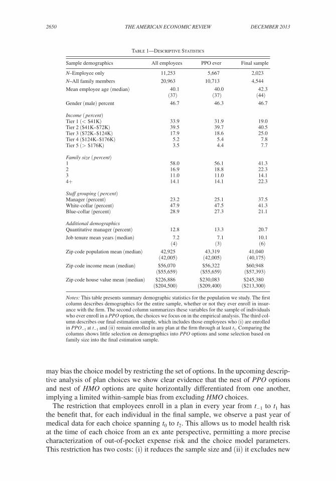
We construct our final sample to leverage the features of the data that allow us to identify inertia. Moving from the full data, we restrict the final sample to employ-ees and dependents who (i) are enrolled in a health plan for all years from t −1 to t 1 and (ii) are enrolled in a PPO option in each of those years (this excludes the employees who enroll in either of two HMO options).10 The second column in Table 1 describes the sample of employees who ever enroll in a PPO option at the firm (N = 5,667), while the third column describes the final sample (N = 2,023). Comparing column 2 to column 1, it is evident that the restriction to PPO options engenders minimal selection based on the rich set of demographics we observe. Comparing both of these columns to column three reveals that the additional restric-tion that employees be enrolled for three consecutive years does lead to some sam-ple selection: employees in the final sample are slightly older, slightly richer, and more likely to cover additional family members than the overall PPO population. Note that the multi-year enrollment restriction primarily excludes employees who enter or exit the firm during this period, rather than those who switch to an HMO option or waive coverage.
There are costs and benefits of these two restrictions. The restriction to PPO plans is advantageous because we observe detailed medical claims data only for enrollees in these plans and these plans are only differentiated by financial characteristics, implying we don’t have to consider heterogeneity in preferences over provider net-work when modeling choice between them. A potential cost is that this restriction
9 These are managers associated with specific groups where the work is highly quantitative in nature.10 We denote all years in reference to t 0 , such that, e.g., year t −1 occurred just before t 0 and year t 1 just after.
2650 THE AMERICAN ECONOMIC REVIEW dECEMbER 2013
may bias the choice model by restricting the set of options. In the upcoming descrip-tive analysis of plan choices we show clear evidence that the nest of PPO options and nest of HMO options are quite horizontally differentiated from one another, implying a limited within-sample bias from excluding HMO choices.
The restriction that employees enroll in a plan in every year from t −1 to t 1 has the benefit that, for each individual in the final sample, we observe a past year of medical data for each choice spanning t 0 to t 2 . This allows us to model health risk at the time of each choice from an ex ante perspective, permitting a more precise characterization of out-of-pocket expense risk and the choice model parameters. This restriction has two costs: (i) it reduces the sample size and (ii) it excludes new
Table 1—Descriptive Statistics
Sample demographics All employees PPO ever Final sample
N–Employee only 11,253 5,667 2,023
N–All family members 20,963 10,713 4,544
Mean employee age (median) 40.1 40.0 42.3 (37) (37) (44)
Gender (male) percent 46.7 46.3 46.7
Income ( percent)Tier 1 (< $41K) 33.9 31.9 19.0Tier 2 ($41K–$72K) 39.5 39.7 40.5Tier 3 ($72K–$124K) 17.9 18.6 25.0Tier 4 ($124K–$176K) 5.2 5.4 7.8Tier 5 (> $176K) 3.5 4.4 7.7
Family size ( percent)1 58.0 56.1 41.32 16.9 18.8 22.33 11.0 11.0 14.14+ 14.1 14.1 22.3
Staff grouping ( percent)Manager (percent) 23.2 25.1 37.5White-collar (percent) 47.9 47.5 41.3Blue-collar (percent) 28.9 27.3 21.1
Additional demographicsQuantitative manager (percent) 12.8 13.3 20.7
Job tenure mean years (median) 7.2 7.1 10.1 (4) (3) (6)
Zip code population mean (median) 42,925 43,319 41,040 (42,005) (42,005) (40,175)
Zip code income mean (median) $56,070 $56,322 $60,948 ($55,659) ($55,659) ($57,393)
Zip code house value mean (median) $226,886 $230,083 $245,380 ($204,500) ($209,400) ($213,300)
Notes: This table presents summary demographic statistics for the population we study. The first column describes demographics for the entire sample, whether or not they ever enroll in insur-ance with the firm. The second column summarizes these variables for the sample of individuals who ever enroll in a PPO option, the choices we focus on in the empirical analysis. The third col-umn describes our final estimation sample, which includes those employees who (i) are enrolled in PP O −1 at t −1 and (ii) remain enrolled in any plan at the firm through at least t 1 . Comparing the columns shows little selection on demographics into PPO options and some selection based on family size into the final estimation sample.
2651handel: adverse selection and inertiavol. 103 no. 7
employees from t 0 to t 2 , who, as the upcoming preliminary analysis section reveals, can provide an additional source of identification for inertia. Ultimately, since the identification within the final sample for inertia is quite strong because of the plan menu change and linked active decision, we feel that having a more precise model is worth the costs of this restriction.11
Health Insurance Choices.—From 2004 to t −1 the firm offered five total health plan options composed of four HMO plans (restricted provider network, greater cost control) and one PPO plan (broader network, less cost control). Each of these five plans had a different network of providers, different contracts with providers, and different premiums and cost-sharing formulas for enrollees. From t 0 on, the new plan menu contained two of the four incumbent HMO plans and three new PPO plans.12 This plan structure remained intact through the end of the data in 2009. After the menu change, the HMOs still had different provider networks and cost sharing rules both relative to each other and to the set of new PPOs. However, the three new PPO plans introduced at t 0 had exactly the same network of providers, the same contractual treatment of providers, and cover the same medical services. The PPO plans are only differentiated from one another (and from the previously offered PPO) by premiums and cost sharing characteristics (e.g., deductible, coin-surance, and out-of-pocket maximums) that determine the mapping from total medi-cal expenditures to employee out-of-pocket expenditures. Throughout the period, all PPO options that the firm offers are self-insured plans where the firm fills the pri-mary role of the insurer and is at risk for incurred claims. We denote the HMO plans available throughout the entire period as HM O 1 and HM O 2 , and those offered only prior to t 0 as HM O 3 and HM O 4 . We denote the PPO option from before the menu change as PP O −1 , while we denote each of the PPO options after the menu change by their respective individual-level deductibles: PP O 250 , PP O 500 , and PP O 1200 .
13 PP O 1200 is paired with a health savings account (HSA) option that allows consumers to deposit tax-free dollars to be used later to pay medical expenditures.14
Table A-2 in online Appendix E presents the detailed characteristics of the PPO plans offered at the firm over time. After the deductible is paid, PP O 250 has a coin-surance rate of 10 percent while the other two plans have rates of 20 percent, imply-ing they have double the marginal price of post-deductible claims. Out-of-pocket maximums indicate the maximum amount of medical expenditures that an enrollee can pay post-premium in a given plan. These are larger the less comprehensive the plan is and vary with income tier. Finally, both PP O 250 and PP O 500 have the same flat-fee co-payment structures for pharmaceuticals and physician office visits, while
11 We could include new employees after t −1 using a less precise cost framework based on, e.g., age, gender, and future claims, similar to what is done in the literature when detailed claims data are not available.
12 An employee who chose a PPO plan at t 0 , by construction, actively chose a new plan. An employee who chose an incumbent HMO prior to t 0 was forced out of that plan and prompted to make an active choice from the new menu, though their old plan remained available. Since we only study PPO plans after t 0 , the incumbent aspect of the HMO plans does not impact our analysis.
13 The deductibles are indicative of how comprehensive (level of insurance) each plan is: for example, PP O 250 provides the most insurance and has the highest premium.
14 This may lead to some horizontal differentiation for PP O 1200 relative to the other two, which we account for in the choice model. This kind of plan is known as a “consumer driven health plan” (CDHP). Employees who signed up for this plan for the first time were given up to a $1,200 HSA match from the firm, which our analysis accounts for.

2652 THE AMERICAN ECONOMIC REVIEW dECEMbER 2013
in PP O 1200 these apply to the deductible and coinsurance.15 Though we model these characteristics at a high-level of detail, our cost model necessarily makes some sim-plifying assumptions that we discuss and validate in online Appendix A.
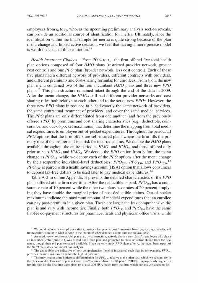
Figure 1, panel A compares plans PP O 250 and PP O 500 graphically, to illustrate the relationship between health plan financial characteristics, total medical expenses, and employee expenses. The figure applies specifically to year t 0 (premiums differ by year) and to low-income families, though it looks similar in structure for other coverage tiers and income levels. It completely represents the in-network differ-ences between these two plans, since they are identical on the dimensions excluded from this chart, such as co-payments for pharmaceuticals and office visits. For this figure, and the rest of our analysis, we assume that (i) premiums are in pre-tax dol-lars and (ii) medical expenses are in post-tax dollars.16 After the employee premium, as total expenditures increase each employee pays the plan deductible, then the flat coinsurance rate, and finally has zero marginal cost after reaching the out-of-pocket maximum.17 As expected, the chart reveals that, ex post, healthy employees should have chosen PP O 500 and sick employees PP O 250 .
Table A-3 in online Appendix E presents details on the pattern of employee choices over time before and after the menu change, which we summarize here. In t −1 , 39 percent of employees enroll in PP O −1 , 47 percent enroll in one of the four HMO options, and 14 percent waive coverage. At t 0 , 46 percent of employees choose one of the three new PPO options, with 25 percent choosing PP O 250 . 37 percent choose either of the two remaining HMO plans while 16 percent waive coverage. Table A-3 also presents clear evidence that the nest of PPO options and nest of HMO options are quite horizontally differentiated from one another by examining consumer health plan transitions over time. An individual who switches plans from a PPO option is much more likely to choose another PPO option than to choose an HMO option. Of the 2,757 employees enrolled in PP O −1 in year t −1 who also enroll in any plan at t 0 , only 85 (3 percent) choose an HMO option at t 0 . In reverse, despite the expansion of PPO options and reduction of HMO options, only 15 percent of employees who chose an HMO option in t −1 , and choose any plan at t 0 , switch to a PPO option. This suggests that restricting the set of choices to PPO options should not lead to biased parameters within that population.
Each plan offered by the firm has a distinct total premium and employee premium contribution in each year. The total premium is the full cost of insurance while the employee premium contribution is the amount the employee actually pays after
15 These characteristics are for in-network purchases: the plans also have out-of-network payment policies, which we do not present or model. The plans have reasonably similar out-of-network payment characteristics (including out-of-pocket maximums). Only 2 percent of realized total expenditures are out-of-network.
16 In reality, medical expenses could also be in pre-tax dollars since individuals can pay medical expenses with pre-tax FSA or HSA contributions. In our data, 25 percent of the population enrolls in these accounts, which fund an even lower percentage of overall employee expenses. We convert premiums into pre-tax dollars by multiplying them by an income and family status contingent combined state and federal marginal tax rate using the NBER TAXSIM data. We may understate marginal tax rates of employees with high-earning spouses, since we don’t observe spousal income.
17 Each family member technically has his or her own deductible and out-of-pocket maximum. Families with 3+ members have aggregate deductible and out-of-pocket caps that bind if multiple family members reach their indi-vidual limits. While we explicitly take this structure into account in our cost model, Figure 1 assumes proportional allocation of expenses across family members.
2653handel: adverse selection and inertiavol. 103 no. 7
2,000
3,000
4,000
5,000
6,000
7,000
8,000
PPO250
PPO500
PPO500 out-of-pocket maximum
Tot
al e
mpl
oyee
exp
ense
s
Panel A. PPO health insurance plan characteristics, t0 low-income family
t0 in-network total medical expenses*
PPO250 out-of-pocket maximum
Coinsurance
Deductible
Premium
Panel B. PPO health insurance plan characteristics, t1 low-income family
2,000
3,000
4,000
5,000
6,000
7,000
8,000
Tot
al e
mpl
oyee
exp
ense
s
1,000
t1 in-network total medical expenses*
PPO250
PPO500
PPO250 out-of-pocket maximum
Coinsurance
PPO500 out-of-pocket maximum
Deductible
Premium
01,
5003,
0004,
5006,
0007,5
009,
000
10,5
00
12,0
00
13,5
00
15,0
00
16,5
00
18,0
00
19,5
00
21,0
00
22,5
00
24,0
00
25,5
00
27,0
00
28,5
00
30,0
00
01,
5003,
0004,
5006,
0007,5
009,
000
10,5
00
12,0
00
13,5
00
15,0
00
16,5
00
18,0
00
19,5
00
21,0
00
22,5
00
24,0
00
25,5
00
27,0
00
28,5
00
30,0
00
Figure 1. Financial Characteristics of PPO250 and PPO500
Notes: This figure describes the relationship between total medical expenses (plan plus employee) and employee out-of-pocket expenses in years t0 and t1 for PPO250 and PPO500. This mapping depends on employee premium, deductible, coinsurance, and out of pocket maxi-mum. This chart applies to low-income families (premiums vary by number of dependents cov-ered and income tier, so there are similar charts for all 20 combinations of these two variables). Premiums are treated as pre-tax expenditures while medical expenses are treated as post-tax. Panel B presents the analogous chart for time t1 when premiums changed significantly, which can be seen by the change in the vertical intercepts. At time t0 healthier employees were bet-ter off in PPO500 and sicker employees were better off in PPO250. At time t1 all employees that this figure applies to should choose PPO500 regardless of their total claim levels, i.e., PPO250 is dominated by PPO500. Despite this, many employees who chose PPO250 in t0 continue to do so at t1, indicative of high inertia.
* Total medical expenses equals plan paid plus employee paid. Ninety-six percent of all expenses are in network.
2654 THE AMERICAN ECONOMIC REVIEW dECEMbER 2013
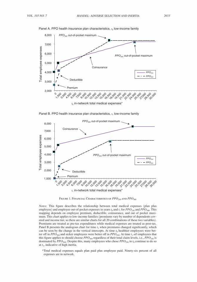
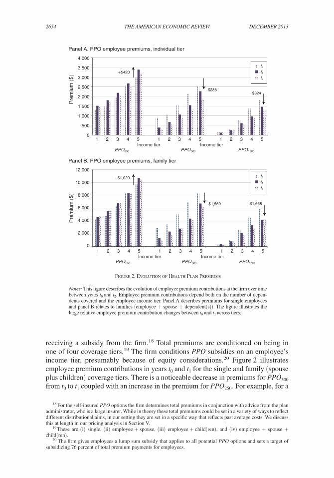
receiving a subsidy from the firm.18 Total premiums are conditioned on being in one of four coverage tiers.19 The firm conditions PPO subsidies on an employee’s income tier, presumably because of equity considerations.20 Figure 2 illustrates employee premium contributions in years t 0 and t 1 for the single and family (spouse plus children) coverage tiers. There is a noticeable decrease in premiums for PP O 500 from t 0 to t 1 coupled with an increase in the premium for PP O 250 . For example, for a
18 For the self-insured PPO options the firm determines total premiums in conjunction with advice from the plan administrator, who is a large insurer. While in theory these total premiums could be set in a variety of ways to reflect different distributional aims, in our setting they are set in a specific way that reflects past average costs. We discuss this at length in our pricing analysis in Section V.
19 These are (i) single, (ii) employee + spouse, (iii) employee + child(ren), and (iv) employee + spouse + child(ren).
20 The firm gives employees a lump sum subsidy that applies to all potential PPO options and sets a target of subsidizing 76 percent of total premium payments for employees.
4,000
3,500
3,000
2,500
2,000
1,500
1,000
500
0
Pre
miu
m ($
)
Panel A. PPO employee premiums, individual tier
1 2 3 4 5 1 2 3 4 5 1 2 3 4 5 Income tier Income tier
PPO250 PPO500 PPO1200
+$420
–$288
t0t1t2
–$324
Panel B. PPO employee premiums, family tier
1 2 3 4 5 1 2 3 4 5 1 2 3 4 5 Income tier Income tier
PPO250 PPO500 PPO1200
12,000
10,000
8,000
6,000
4,000
2,000
0
Pre
miu
m ($
)
+$1,020
–$1,560
t0t1t2
–$1,668
Figure 2. Evolution of Health Plan Premiums
Notes: This figure describes the evolution of employee premium contributions at the firm over time between years t0 and t2. Employee premium contributions depend both on the number of depen-dents covered and the employee income tier. Panel A describes premiums for single employees and panel B relates to families (employee + spouse + dependent(s)). The figure illustrates the large relative employee premium contribution changes between t0 and t1 across tiers.
2655handel: adverse selection and inertiavol. 103 no. 7
family in the top income tier, the price of PP O 500 decreased by $1, 560 from t 0 to t 1 while the price of PP O 250 increased by $1, 020.21 There are also substantial relative premium changes for the other three coverage tiers. As a result of these large rela-tive employee premium changes, the choice setting in year t 1 , when most employees had a default option and inertia, is quite different than that in t 0 when the forced re-enrollment occurred.
II. Preliminary Analysis
We start the analysis by presenting some descriptive evidence of inertia and adverse selection. We investigate two different model-free tests that suggest inertia is an important factor in determining choices over time. In addition, we present a test for adverse selection based on the data alone. While this section presents strong evidence on the existence and potential impact of these two phenomena, it also high-lights that a more in depth modeling exercise is essential to precisely quantify their magnitudes and evaluate the impact of a counterfactual reduction in inertia. Each analysis uses a sample that differs from our primary sample because of the specific source of identification involved.
New Employees.—Our first test for inertia studies the behavior of new employees at the firm over time. New employees are an interesting group to investigate because they have no inertia when they choose a new health plan at the time of their arrival. This is because (i) they have no health plan default option at the time of arrival and (ii) they were not previously enrolled in any health plan within the firm.22 Thus, in our setting, employees who are new for year t 0 have no inertia in that period and positive inertia when choosing a plan for year t 1 . Moving forward, employees who are new in year t 1 have no inertia at t 1 and positive inertia thereafter. Given the large price changes for t 1 described in the prior section, if the profile of new employees is similar in each year then large inertia should imply that the t 1 choices of new enrollees at t 0 are different than the t 1 choices of new enrollees at t 1 . In that case, the t 1 choices of t 0 new enrollees should reflect the choice environments at both t 0 and t 1 , while the t 1 choices of t 1 new enrollees should depend on just the t 1 environment.
Table 2 compares the choices over time of the cohorts of new enrollees from years t −1 , t 0 , and t 1 , with each group composed of slightly more than 1,000 employees. Without inertia, we would expect the choices in these three cohorts to be the same at t 1 , since the table reveals that they are virtually identical on all other demographic dimensions, including age, gender, income, FSA enrollment, and health expendi-tures. Instead, while it is evident that the t 0 and t −1 cohorts make very similar choices with the default option at t 1 , the new enrollees making active choices in that year have a very different choice profile that reflects the price changes for t 1 . For example, 21 percent of t 0 new enrollees choose PP O 250 at t 0 while 23 percent choose PP O 500 . At t 1 , 20 percent of this cohort choose PP O 250 and 26 percent choose PP O 500 only a
21 This movement is due to total premium adjustment based on t 0 average costs for each plan and coverage tier, reflecting adverse selection against PP O 250 .
22 Since each PPO option we study has the exact same network of providers, there is no built-in advantage for specific plans because of prior coverage. Further, since the PPO options are self-insured, these specific plans are not offered in the same names and formats at other firms or in the private market.
2656 THE AMERICAN ECONOMIC REVIEW dECEMbER 2013
small change in market share for each plan in the direction expected given the price changes. The decision profile over time for new enrollees at t −1 is similar. However, new enrollees at t 1 choose PP O 250 only 11 percent of the time, while choosing PP O 500 43 percent of the time. This implies that t 0 and t −1 new employees made active choices at t 0 and only adjusted slightly to large price changes at t 1 , due to significant inertia, while t 1 new employees with no t 1 inertia made active choices at t 1 , reflecting the current prices.
Dominated Plan Choice.—Our second test for inertia leverages a specific situ-ation caused by the combination of plan characteristics and plan price changes in our setting. As a result of the large price changes for year t 1 , PP O 250 became strictly
Table 2—New Employee Health Plan Choices
New enrollee analysis New enrollee t −1 New enrollee t 0 New enrollee t 1
N, t 0 1,056 1,377 —N, t 1 784 1,267 1,305
t 0 ChoicesPP O 250 259 (25%) 287 (21%) —PP O 500 205 (19%) 306 (23%) —PP O 1200 155 (15%) 236 (17%) —HM O 1 238 (23%) 278 (20%) —HM O 2 199 (18%) 270 (19%) —
t 1 ChoicesPP O 250 182 (23%) 253 (20%) 142 (11%)PP O 500 201 (26%) 324 (26%) 562 (43%)PP O 1200 95 (12%) 194 (15%) 188 (14%)HM O 1 171 (22%) 257 (20%) 262 (20%)HM O 2 135 (17%) 239 (19%) 151 (12%)
DemographicsMean age 33 33 32Median age 31 31 31Female percent 56% 54% 53%Manager percent 20% 18% 19%FSA enroll percent 15% 12% 14%Dental enroll percent 88% 86% 86%Median (mean) expense t 1 844 (4,758) 899 (5,723) —
Income tier 1 48% 50% 47%Income tier 2 33% 31% 32%Income tier 3 10% 10% 12%Income tier 4 5% 4% 4%Income tier 5 4% 5% 5%
Notes: This table describes the choice behavior of new employees at the firm over several con-secutive years and presents our first model-free test of inertia. Each column describes one cohort of new employees at the firm, corresponding to a specific year of arrival. First, the chart describes the health insurance choices made by these cohorts in year t 0 (the year of the insurance plan menu change) and in the following year, t 1 . The last part of the chart lists the demographics for each cohort of new arrivals at the time of their arrival. Given the very similar demographic pro-files and large sample size for each cohort, if there is no inertia, the t 1 choices of employees who entered the firm at t 0 and t −1 should be very similar to the t 1 choices of employees who entered the firm at t 1 . The table shows that, in fact, the active choices made by the t 1 cohort are quite different than those of the prior cohorts in the manner we would expect with high inertia: the t 1 choices of employees who enter at t 0 and t −1 reflect both t 1 prices and t 0 choices while the t 1 choices of new employees at t 1 reflect t 1 prices.
2657handel: adverse selection and inertiavol. 103 no. 7
dominated for certain combinations of family size and income, which determine employee premium contributions. Strict dominance implies that for any possible level and type of total medical expenditures, PP O 500 leads to lower employee expen-ditures (premium plus out-of-pocket) than PP O 250 . Figure 1, panel B reproduces, for year t 1 , the t 0 analysis of PP O 250 and PP O 500 health plan characteristics discussed earlier. The figure studies the relationship between total medical expenditures and employee expenditures for low-income families. For this group, the large relative premium change between these two plans for t 1 shifts the relative baseline employee expenditures so much that a low-income family should always enroll in PP O 500 at t 1 if making an active choice, regardless of beliefs about future medical expenditures. In fact, the figure illustrates that a low-income family that enrolls in PP O 250 at t 1 must lose at least $1,000 relative to PP O 500 . Recall that this chart represents all dimen-sions of differentiation between these two plans. At t 0 , with the active re-enrollment, no plans were dominated for any employee. PP O 250 is dominated at t 1 for four of the other nineteen potential coverage and income tier combinations. It is important to note that the existence of dominated plans for these select groups was unknown to the firm at t 1 . The firm determined total premiums and subsidies over time separately from the t 0 decision on health plan characteristics, such that the firm did not analyze these features in combination with each other at t 1 and t 2 as we do here.
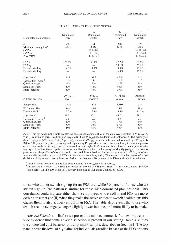
Table 3 describes the behavior of the subset of employees who enrolled in PP O 250 at t 0 and had that plan become dominated for them in t 1 and t 2 . Of the 1,897 employ-ees who enroll in PP O 250 at t 0 and remain with the firm at t 1 , 559 (29 percent) had that plan become dominated for them in t 1 (504 of these remain at the firm for t 2 ). Of these 559 employees, only 61 (11 percent) switch plans to an undominated plan at t 1 indicating substantial persistence in plan choice that must, at least in part, be the result of inertia because unobserved preference heterogeneity cannot fully rational-ize choosing PP O 250 at t 1 . Thus, for these employee groups, in a rational frictionless environment we would expect 100 percent of the individuals enrolled in PP O 250 at t 0 to switch to PP O 500 at t 1 . Of the 61 employees that did switch at t 1 , the majority (44 (72 percent)) switch to PP O 500 as expected given the large relative price drop of that plan. This pattern remains similar even at t 2 after employees have had more time to communicate with one another: only 126 (25 percent) of the 504 employees switch by t 2 , with 103 (82 percent) switching to PP O 500 . The table reveals that the average minimum money lost by these employees from staying in PP O 250 is $374 at t 1 and $396 at t 2 .
Table 3 also reveals that employees who switch plans over time are more likely to make other active decisions. The top part of the table describes linked FSA and dental plan decisions for those with dominated plans, while the bottom panel describes these choices for people who switch from any PPO option in the entire population. Conditional on switching from a dominated option at t 1 , 14.1 percent of employees also switch dental plans at t 1 , compared to 4.3 percent for those who do not switch. For the entire population in PPO plans (3,170 employees present over multiple years) the analogous numbers switching dental plans are 14.5 percent and 3.8 percent. Further, employees who switch plans at t 1 are more likely to enroll in an FSA at t 1 . This is a relevant choice to study because FSA enrollment is an active choice in each year: employees who do not actively elect to sign up and list a contri-bution level are not enrolled. For the entire population in PPO plans, 25 percent of
2658 THE AMERICAN ECONOMIC REVIEW dECEMbER 2013
those who do not switch sign up for an FSA at t 1 while 39 percent of those who do switch sign up (the pattern is similar for those with dominated plan options). This correlation could indicate either that (i) employees who enroll in and FSA are more active consumers or (ii) when they make the active choice to switch health plans this causes them to also actively enroll in an FSA. The table also reveals that those who switch are, on average, younger, slightly lower income, and more likely to be male.
Adverse Selection.—Before we present the main econometric framework, we pro-vide evidence that some adverse selection is present in our setting. Table 4 studies the choice and cost behavior of our primary sample, described in Section I. The top panel shows the level of t −1 claims for individuals enrolled in each of the PPO options
Table 3—Dominated Plan Choice Analysis
Dominated plan analysis
t 1 Dominated
stay
t 1 Dominated
switch
t 2 Dominated
stay
t 2 Dominated
switch
N 498 61 378 126Minimum money losta $374 $453 $396 $306PP O 500 — 44 (72%) — 103 (81%)PP O 1200 — 4 (7%) — 6 (5%)Any HMO — 13 (21%) — 17 (14%)
FSA t 1 25.4% 32.1% 27.2% 28.6%FSA t 2 — — 28.1% 30.9%Dental switch t 1 4.3% 14.1% 3.5% 10.9%Dental switch t 2 — — 6.9% 17.2%
Age (mean) 44.9 38.3 46.2 41.4Income tier (mean)b 1.6 1.4 1.6 1.7Quant. manager 11% 8% 11% 11%Single (percent) 40% 41% 40% 33%Male (percent) 42% 46% 39% 55%
All plan analysisPP O 250 stay t 1
PP O 250 switch t 1
All plans t 1 stay
All plans t 1 switch
Sample size 1,626 174 2,786 384FSA t 1 enrollee 31% 41% 25% 39%Dental switch 3.2% 13.1% 3.8% 14.5%
Age (mean) 48.3 40.6 44.0 39.1Income tier (mean)b 2.5 2.2 2.3 2.1Quant. manager 20% 17% 17% 14%Single (percent) 50% 56% 53% 59%Male (percent) 48% 42% 49% 40%
Notes: This top panel in this table profiles the choices and demographics of the employees enrolled in PPO250 at t 0 who (i) continue to enroll in a firm plan in t 1 and (ii) have PPO250 become dominated for them at t 1 . The majority of these employees (498 out of 559 (89 percent)) remain in PPO250 even after it becomes dominated by PPO500 with 378 of 504 (25 percent) still remaining in this plan at t 2 . People who do switch are more likely to exhibit a pattern of active choice behavior in general as evidenced by their higher FSA enrollments and level of dental plan switch-ing. Apart from this, these populations are similar though switchers in this group are slightly younger. The bottom panel studies the profiles of those who switch at t 1 and those who don’t for the two groups of (i) PPO250 enrollees at t 0 and (ii) the entire universe of PPO plan enrollees present in t 0 and t 1 . This reveals a similar pattern of active decision making as switchers in these populations are also more likely to enroll in FSAs and switch dental plans.
a Mean of lower bound on money lost from enrolling in PP O250 instead of PPO500 . b Income tier has values 1–5 where 1 is lowest income and 5 is highest. Tiers 1–4 are approximately $40,000
increments, starting at 0, while tier 5 is everything greater than approximately $175,000.

2659handel: adverse selection and inertiavol. 103 no. 7
from t −1 to t 1 . We study t −1 claims for plans chosen across all three years t −1 to t 1 to avoid the potential alternative explanation of moral hazard: in year t −1 all families in this sample were enrolled in PP O −1 implying that t −1 claims are an “apples to apples” measure of health expense risk. The table reveals that there is selection on medical expenses against the most comprehensive plan, PP O 250 . Employees who chose PP O 250 had almost double the median and mean of t −1 total medical claims relative to enrollees in the other two PPO options, in both t 0 and t 1 . Despite the large price change from t 0 to t 1 , the pattern of selection barely changes over these years. The high level of selection at t 0 reveals that consumers initially chose plans based on health risk, while the lack of movement in selection over time implies that indi-viduals did not update their selection over time, even though prices changed signifi-cantly. This motivates our counterfactual exercise investigating the impact of polices that reduce inertia in the context of a setting with adverse selection.
Table 4 —Adverse Selection and Employee Costs
Final sample total expenses PP O −1 PP O 250 PP O 500 PP O 1200
Family t −1 total expenses ($) t −1 N employees (mean family size) 2,022 (2.24) — — — Mean (median) 13,331 (4,916) — — — 25th percentile 1,257 — — — 75th percentile 13,022 — — —
t 0 N (mean family size) — 1,328 (2.18) 414 (2.20) 280 (2.53) Mean (median) — 16,976 (6,628) 6,151 (2,244) 6,742 (2,958) 25th percentile — 2,041 554 658 75th percentile — 16,135 6,989 8,073
t 1 N (mean family size) — 1,244 (2.19) 546 (2.19) 232 (2.57) Mean (median) — 17,270 (6,651) 7,759 (2,659) 6,008 (2,815) 25th percentile — 2,041 708 589 75th percentile — 16,707 8,588 7,191
Individual category expenses (dollars)Pharmacy Mean 973 1,420 586 388 Median 81 246 72 22
Mental health ( > 0) Mean 2,401 2,228 1,744 2,134 Median 1,260 1,211 1,243 924
Hospital/physician Mean 4,588 5,772 2,537 2,722 Median 428 717 255 366
Physician OV Mean 461 571 381 223 Median 278 356 226 120
Notes: This table investigates the extent of adverse selection across PPO options after the t 0 menu change for those in the final estimation sample. All individuals in this sample were enrolled in PPO−1 in t−1 and continue to be enrolled in some plan at the firm for the following two years. The numbers in the table for all choices represent t−1 total claims in dollars so that these costs can proxy for health risk without being confounded by moral hazard (t0 and t1 cost differences could be the result of selection or moral hazard). The table reveals that those who choose PPO250 have much higher expenditures at t−1 than those who choose the other two plans, implying substantial selection on observables in the vein of Finkelstein and Poterba (2006). The bottom panel presents a breakdown of these costs according to our cost model expenditure categories.
2660 THE AMERICAN ECONOMIC REVIEW dECEMbER 2013
III. Empirical Framework
The analysis in the previous section provides evidence of both substantial inertia and adverse selection without imposing specific choice and cost models. This sec-tion presents a model of consumer choice with three primary components: (i) iner-tia, (ii) risk preferences, and (iii) ex ante cost projections. We describe the empirical implementation of this model, which links the choice and medical cost data we observe to these underlying economic choice fundamentals. Relative to the earlier analysis, this framework makes it possible to (i) quantify inertia and (ii) determine the impact of potential counterfactual policies that reduce inertia. These additional conclusions should be viewed in the context of the structural assumptions included in the model. We present the supply-side insurance pricing model later in Section V, together with the analysis of the interaction between inertia and adverse selection.
Choice Model.—We describe the model in two components. First we describe the choice framework conditional on predicted family-level ex ante medical cost risk. Next, we describe the detailed cost model that generates these expenditure distributions.
The choice model quantifies inertia and risk preferences conditional on the family-plan-time specific distributions of out-of-pocket health expenditures output by the cost model. Denote these expense distributions F kjt ( ⋅ ), where k ∈ is a family unit, j ∈ is one of the three PPO insurance plans available after the t 0 menu change, and t ∈ is one of three years from t 0 to t 2 . We assume that families’ beliefs about their out-of-pocket expenditures conform to F kjt ( ⋅ ). Each family has latent utility U kjt for each plan in period t. In each time period, each family chooses the plan j ∈ that maximizes U kjt . We use what Einav, Finkelstein, and Levin (2010) call a “real-ized” empirical utility model and assume that U kjt has the following von-Neuman Morgenstern (v-NM) expected utility formulation:
U kjt = ∫ 0 ∞ f kjt (OOP) u k ( W k , OOP, P kjt , 1 kj, t−1 ) dOOP.
Here, u k ( ⋅ ) is the v-NM utility index and OOP is a realization of medical expenses from F kjt ( ⋅ ). W k denotes family-specific wealth. P kjt is the family-time specific premium contribution for plan j, which depends both on how many dependents are covered and on employee income. 1 kj, t−1 is an indicator of whether the family was enrolled in plan j in the previous time period.
We assume that families have constant absolute risk aversion (CARA) prefer-ences implying that for a given ex post consumption level x:
u k (x) = − 1 _ γ k ( X k A )
e − γ k ( X k A ) x .
Here, γ k is a family-specific risk preference parameter that is known to the family but unobserved to the econometrician. We model this as a function of employee demographics X k A . As γ increases, the curvature of u increases and the decision
2661handel: adverse selection and inertiavol. 103 no. 7
maker is more risk averse. The CARA specification implies that the level of absolute risk aversion
−u″( ⋅ ) _ u′ ( ⋅ ) , which equals γ, is constant with respect to the level of x.23
In our primary empirical specification a family’s overall level of consumption x conditional on a draw OOP from F kjt ( ⋅ ) depends on multiple factors:
x = W k − P kjt − OOP + η( X kt B , Y k ) 1 kj, t−1 + δ k ( Y k ) 1 1200 + α H k, t−1 1 250 + ϵ kjt ( Y k ).
We model inertia, represented by η, as an implied monetary cost, similar in struc-tural interpretation to a tangible switching cost. Inertia depends on the observed linked choice and demographic variables X kt B
and Y k , described in more detail in the estimation section. δ k is an unobserved family-specific plan intercept for PP O 1200 ( 1 1200 is an indicator for j = PP O 1200 at t for family k). On average, we expect δ k to differ from zero because the health savings account (HSA) option offered exclu-sively through PP O 1200 horizontally differentiates this plan from the other two PPO options.24 α measures the intrinsic preference of a high-cost family for PP O 250 , where high-cost, represented by the binary variable H k, t−1 , is defined as greater than the ninetieth percentile of the total cost distribution (≈ $27, 000 ).25 Finally, ϵ kjt rep-resents a family-plan-time specific idiosyncratic preference shock. Since the plans we study are only differentiated by financial characteristics (apart from the HSA feature) we also follow Einav et al. (2013) and study a robustness check with no idiosyncratic preference shock.
There are several assumptions in the choice model that warrant additional discus-sion. First, inertia is modeled in a specific way, as an incremental cost paid condi-tional on switching plans. This framework implies that, on average, for a family to switch at t they must prefer an alternative option by $η more than their default. This follows the approach used in prior empirical work that quantifies switching costs (e.g., Shum 2004 or Dube et al. 2008), which also does not distinguish between micro-foundations of inertial behavior. It is unlikely that this specification for inertia significantly impacts other parameter estimates (such as risk preferences) because those parameters are identified separately from inertia, in any form, in the active choice year at t 0 . A choice model estimated only on t 0 choices would yield similar estimates regardless of how inertia is specified. Further, while alternative specifica-tions would capture the evident persistence in plan choice with different underlying mechanisms, we argue in our upcoming analysis of inertia reduction in Section V that their implications for how inertia interacts with adverse selection would not differ
23 This implies that wealth W k does not impact relative plan utilities. As a result, it drops out in estimation. The measure for wealth would matter for an alternative model such as constant relative risk aversion (CRRA) preferences.
24 Prior work shows that HSAs can cause significant hassle costs or provide an extra benefit in the form of an additional retirement account (see, e.g., Reed et al. 2009 or McManus et al. 2006). Consumer uncertainty about how HSAs function could also deter choice of the high-deductible plan. We subsume potential/actual observed HSA contributions and employer contribution matches for first-time enrollees into δ k in lieu of a more detailed model.
25 This is included to proxy for the empirical fact that almost all families with very high expenses choose PP O 250 whether it is the best plan for them or not. These families may assume that, given their high expenses, they should always choose the most comprehensive insurance option.

2662 THE AMERICAN ECONOMIC REVIEW dECEMbER 2013
substantially from those of our primary model.26 We present a detailed discussion of sources of inertia and their implications for this analysis in online Appendix D.
Additionally, the model assumes that families know the distribution of their future health expenditure risk and that this risk conforms to the output of the cost model described in the next section. This assumption could be incorrect for at least two reasons. First, families may have private information about their health statuses that is not captured in the detailed prior claims data. Second, families may have less information about their projected future health expenditures: the cost model utilizes a full profile of past claims data in conjunction with medical software that maps past claims to future expected expenses. Further, the model contains the assumption that consumers have full knowledge of health plan characteristics and incorporate that knowledge into their decision process. Each of these possible deviations implies a potential bias in F kjt . Along with our main results, we present a robustness analysis to show that reasonable sized deviations from our estimates of F kjt do not substan-tially affect the estimates of inertia or other choice model parameters.
Finally, the model assumes that consumers are myopic and do not make dynamic decisions whereby current choices would take into account inertia in future periods. There are several arguments to support this approach. First, price changes are not signaled in advance and change as a function of factors that would be difficult for consumers to model.27 Second, it is unlikely that most consumers can forecast sub-stantial changes to their health statuses more than one year in advance. Third, in this empirical setting consumers make initial choices that make little sense in the context of a fully dynamic approach with accurate beliefs about future prices. They choose (and stay with) plans at t 0 that provide poor long run value given the time path of prices and health expectations.
Cost Model.—The choice framework presented in the previous section takes the distribution of future out-of-pocket expenditures for each family, health plan, and time period, F kjt ( ⋅ ), as given. This section summarizes the empirical model we use to estimate F kjt ( ⋅ ). Online Appendix A presents a more formal description of the model, its estimation algorithm, and its results.
Our approach models health risk and out-of-pocket expenditures at the individual level, and aggregates the latter measure to the family level since this is the rel-evant metric for plan choice. For each individual and choice period, we model the distribution of future health risk at the time of plan choice using past diagnostic, demographic, and cost information. This ex ante approach to the cost model fits naturally with the insurance choice model where families make plan choices under uncertainty. In the majority of prior work investigating individual-level consumer choice and utilization in health insurance, health risk is either modeled based on (i) demographic variables such as age and gender and/or (ii) aggregated medical cost data at the individual level, from past or futures years (Carlin and Town 2009,
26 These arguments do not address whether overcoming inertia represents a tangible cost from a welfare perspec-tive. Our analysis in Section V takes this into account by studying welfare implications over the range of cases from full inclusion (inertia represents a tangible cost) to no inclusion (only the impact of inertia on choices matters).
27 For consumers to understand the evolution of prices they would have to (i) have knowledge of the pricing model, (ii) have knowledge about who will choose which plans, and (iii) have knowledge about other employees’ health.

2663handel: adverse selection and inertiavol. 103 no. 7
Einav et al. 2013, and Abaluck and Gruber 2011 are notable exceptions). While these approaches are useful approximations when detailed medical data are not available, our model is able to more precisely characterize a given family’s informa-tion set at the time of plan choice and can be linked directly to the choice problem.
The model is set up as follows:
(i) For each individual and open enrollment period, we use the past year of diag-noses (ICD-9), drugs (NDC), and expenses, along with age and gender, to predict mean total medical expenditures for the upcoming year. This pre-diction leverages the Johns Hopkins ACG Case-Mix software package and incorporates medically relevant metrics such as type and duration of specific conditions, as well as co-morbidities.28 We do this for four distinct types of expenditures: (i) pharmacy, (ii) mental health, (iii) physician office visit, and (iv) hospital, outpatient, and all other.
(ii) We group individuals into cells based on mean predicted future utilization. For each expenditure type and risk cell, we estimate a spending distribu-tion for the upcoming year based on ex post observed cost realizations. We combine the marginal distributions across expenditure categories into joint distributions using empirical correlations and copula methods.
(iii) We reconstruct the detailed plan-specific mappings from total medical expenditures to plan out-of-pocket costs. This leverages the division into four expenditure categories, which each contributes uniquely to this map-ping. We combine individual total expense projections into the family out-of-pocket expense projections used in the choice model, F kjt , taking into account family-level plan characteristics.
The cost model assumes that there is no private information and no moral haz-ard (total expenditures do not vary with j ). While both of these phenomena have the potential to be important in health care markets, and are studied extensively in other research, we believe that these assumptions do not materially impact our results. One primary reason is that both effects are likely to be quite small relative to the estimated value lost due to inertia (above a thousand dollars on average). For private information, we should be less concerned than prior work because our cost model combines detailed individual-level prior medical utilization data with sophisticated medical diagnostic software. This makes additional selection based on private information much more unlikely than it would be in a model that uses coarse demographics or aggregate health information to measure health risk.29 For moral hazard, Chandra, Gruber, and McKnight (2010) present a recent review of
28 For example, in our model, a 35-year-old male who spent $10,000 on a chronic condition like diabetes in the past year would have higher predicted future health expenses than a 35-year-old male who spent $10,000 in the past year to fix a time-limited acute condition, such as a broken arm.
29 Pregnancies, genetic pre-dispositions, and non-coded disease severity are possible examples of private informa-tion that could still exist. Cardon and Hendel (2001) find no evidence of selection based on private information with coarser data while Carlin and Town (2009) use similarly detailed claims data and also argue that significant residual selection is unlikely. Importantly, it is also possible that individuals know less about their risk profiles than we do.
2664 THE AMERICAN ECONOMIC REVIEW dECEMbER 2013
the experimental and quasi- experimental literature, where the price elasticity for medical care generally falls in the range −0.1 to −0.4. Recent work by Einav et al. (2013), with data similar to that used here, finds an implied elasticity of −0.14. We perform an in-depth robustness analysis in the next section that incorporates these elasticity estimates into our cost model estimates to verify that the likely moral haz-ard impact (i) is small relative to the degree of inertia we measure and (ii) does not markedly impact our parameter estimates.30
Identification.—Our primary identification concern is to separately identify inertia from persistent unobserved preference heterogeneity. Prior studies seeking to quantify inertia have been unable to cleanly distinguish between these phe-nomena primarily because, in their respective settings, they (i) do not observe consumers making identifiably “active” choices in some periods and identifiably “passive” choices in others while (ii) the products in question are differentiated such that persistent consumer preference heterogeneity is a distinct entity for each product (see Dube, Hitsch, and Rossi 2010 for a discussion). We leverage three features of the data and environment to identify inertia. First, the plan menu change and forced re-enrollment at year t 0 ensures that we observe each family in our final sample making both an “active” and a “passive” choice from the same set of health plans over time, in the context of meaningful relative price changes. Second, the three PPO plan options we study have the exact same network of medical providers and cover the same medical services, implying that differentia-tion occurs only through preferences for plan financial characteristics (here, risk preferences). Third, since insurance choice here is effectively a choice between different financial lotteries, our detailed medical data allow us to precisely quan-tify health risk and the ex ante value consumers should have for health plans, con-ditional on risk preferences and the assumption that beliefs conform to F kjt . Thus, we identify consumer preference heterogeneity based on the choices made at t 0 , while we identify inertia based on choice movement over time as predicted plan values change due to price and health status changes.
We separately identify the two sources of persistent preference heterogeneity γ (risk preferences) and δ (PP O 1200 differentiation) by leveraging the structure of the three available choices. γ is identified by the choice between PP O 250 and PP O 500 , which are not horizontally differentiated, and δ is identified by examining the choice between the nest of those two plans and PP O 1200 .
Estimation.—In our primary specification, we assume that the random coefficient γ k is normally distributed with a mean that is linearly related to observable charac-teristics X k A :31
γ k ( X k A ) → N ( μ γ ( X k A ), σ γ 2 )
μ γ ( X k A ) = μ + β ( X k A ) .
30 A prior version of this paper presented descriptive evidence, similar in spirit to the correlation test in Chiappori and Salanie (2000), suggesting limited selection on private information and moral hazard in our setting.
31 For normally-distributed γ, we assume that γ is truncated just above zero.
2665handel: adverse selection and inertiavol. 103 no. 7
In the primary specification X k A contains employee age and income. We also inves-tigate a robustness check with log-normally distributed γ. We denote the mean and variance of δ k , the random intercept for PP O 1200 , as μ δ ( Y k ) and σ δ 2 ( Y k ). These quanti-ties are estimated conditional on the binary family status indicator Y k , with the two categories of (i) single and (ii) family covering dependents.32
Inertia, η( X kt B , Y k ), is related linearly to Y k and linked choices and demographics
X kt B :
η( X kt B , Y k ) = η 0 + η 1 X kt B
+ η 2 Y k .
X kt B contains potentially time-varying variables that inertia may depend on, including
income and whether or not (i) the family enrolls in an FSA, (ii) the employee has a quantitative background, (iii) the employee is a manager within the firm, (iv) a family member has a chronic medical condition, (v) the family has a large change in expected expenditures from one year to the next, and (vi) the family switches away from PP O 1200 . Many of the X kt B
conditioning variables, as well as Y k , are binary, implying the linearity assumption is not restrictive for them.
Finally, we assume that the family-plan-time specific error terms ϵ kjt are i.i.d. normal for each j with zero mean and variances σ ϵ j
2 ( Y k ). Since Y k is binary we make
no additional assumptions on how these variances relate to Y k . We normalize the value of ϵ 250 , the preference shock for PP O 250 , to zero for each realization of Y k , and estimate the preference shock variances for the other two plans relative to PP O 250 .
33 Since the set of PPO plans we study can be compared purely on financial charac-teristics (conditional on the modeled PP O 1200 differentiation), we follow Einav et al. (2013) and study a robustness specification without ϵ kjt .
We estimate the choice model using a random coefficients simulated maximum likelihood approach similar to that summarized in Train (2009). The likelihood function at the family level is computed for a sequence of choices from t 0 to t 2 , since inertia implies that the likelihood of a choice made in the current period depends on the previous choice. Since the estimation algorithm is similar to a standard approach, we describe the remainder of the details in online Appendix B.
IV. Choice Model Results
Table 5 presents the results of the choice model. Column 1 presents the results from the primary specification while columns 2–5 present the results from four robustness analyses.
In the primary specification, the inertia value intercept η 0 is large in magnitude with values of $1,729 for single employees and of $2,480 for employees who cover at least one dependent. An employee who enrolls in a flexible spending account (FSA) is estimated to forgo $551 less due to inertia than one who does not. The results show a small and negative relationship between income tier and inertia.
32 While age, income, and family status do change over time, they vary minimally over the three-year estimation period so we treat them as fixed over time here. We use the average value of the individual employee who is choos-ing insurance for each family for age and income, and the modal value over time for family status.
33 Since the model is a “realized” utility model in dollar units, we don’t need an ϵ variance scale normalization.

2666 THE AMERICAN ECONOMIC REVIEW dECEMbER 2013
Table 5—Choice Model Parameter Estimates
Empirical model resultsParameter Primary Two plan MH robust γ Robust ϵ Robust
Inertia—single, η 0 1,729 1,686 1,859 2,430 1,944 (28) (82) (107) (116) (150)
Inertia—family, η 0 + η 2 2,480 2,401 2,355 3,006 2,365 (26) (73) (113) (94) (34)
Inertia—FSA enroll, η 1 −551 −355 −669 −723 −417 (56) (78) (155) (131) (50)
Inertia—income, η 1 −32 −130 −59 −8 −7 (13) (22) (15) (43) (15)
Inertia—quantitative, η 1 5 −122 −40 −537 −6 (138) (110) (80) (223) (92)
Inertia—manager, η 1 198 464 277 875 224 (292) (106) (164) (200) (244)
Inertia—chronic condition, η 1 80 26 29 −221 67 (46) (72) (67) (148) (35)
Inertia—salient change, η 1 156 13 95 61 123 (83) (102) (60) (212) (54)
Inertia—PP O 1200 , η 1 −19 — −32 −327 −113 (184) — (46) (122) (52)
Inertia—total pop. mean, η 2,032 1,802 1,886 1,914 1,986 [pop. standard deviation] [446] [416] [387] [731] [316]
Risk aversion mean— 2.32 × 1 0 −4 3.25 × 1 0 −4 2.31 × 1 0 −4 −8.94 1.90 × 1 0 −4
intercept, μ γ ( 9.0 × 1 0 −6 ) (2.2 × 1 0 −5 ) (1.1 × 1 0 −5 ) (0.43) (1.0 × 1 0 −5 ) Risk aversion mean—income, β 2.90 × 1 0 −5 6.11 × 1 0 −5 1.80 × 1 0 −5 0.07 2.40 × 1 0 −5
( 4.0 × 1 0 −6 ) (9.0 × 1 0 −6 ) (3.0 × 1 0 −6 ) (0.016) (3.0 × 1 0 −6 ) Risk aversion mean—age, β 2.27 × 1 0 −6 7.16 × 1 0 −6 3.45 × 1 0 −6 0.28 2.59 × 1 0 −6
( 1.7 × 1 0 −7 ) (4.6 × 1 0 −7 ) (1.8 × 1 0 −7 ) (0.011) (1.5 × 1 0 −7 ) Risk aversion standard 1.88 × 1 0 −4 4.06 × 1 0 −4 1.27 × 1 0 −4 1.37 1.04 × 1 0 −4
deviation, σ γ ( 6.6 × 1 0 −5 ) (2.3 × 1 0 −5 ) (6.0 × 1 0 −6 ) (0.06) (5.9 × 1 0 −5 )
CDHP—single—RC mean, δ −2,912 — −2,801 −2,985 −2,833 (754) — (416) (85) (130)
CDHP—single—RC 843 — 1,070 989 1,141
SD, σ δ (431) — (139) (70) (113)CDHP—family—RC mean, δ −2,871 — −2,614 −5,344 −2,932
(73) — (115) (134) (40)CDHP—family—RC 897 — 1,149 2,179 1,013
SD, σ δ (28) — (132) (80) (31)High total cost—PP O 250 , α 856 763 607 1,386 860
(50) (55) (55) (264) (66) ϵ 500 , σ—single 204 57 51 50 —
(13) (25) (30) (55) —
ϵ 1200 , σ—single 502 — 647 161 — (475) — (228) (72) —
ϵ 500 , σ—family 329 590 789 90 —(25) (68) (28) (89) —
ϵ 1200 , σ—family 811 — 715 676 — (25) — (44) (426) —
Notes: This table presents the estimated parameter results for the primary choice model from Section III and the four robustness checks outlined in Section IV. All non-risk aversion coefficients are in dollar units with standard errors for parameters given in parentheses. The results from the Primary specification are the inputs into the coun-terfactual simulations presented in Section VI.
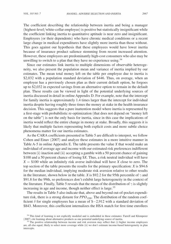
2667handel: adverse selection and inertiavol. 103 no. 7
The coefficient describing the relationship between inertia and being a manager (highest -level/white-collar employee) is positive but statistically insignificant while the coefficient linking inertia to quantitative aptitude is near zero and insignificant. Employees (or their dependents) who have chronic medical conditions or a recent large change in medical expenditures have slightly more inertia than those without. This goes against our hypothesis that these employees would have lower inertia because of insurance product salience stemming from recent increased attention. However, these employees are predominantly high-cost consumers who also may be unwilling to switch to a plan that they have no experience using.34
Since our estimates link inertia to multiple dimensions of observable heteroge-neity, we also present the population mean and variance of inertia implied by our estimates. The mean total money left on the table per employee due to inertia is $2,032 with a population standard deviation of $446. Thus, on average, when an employee has a previously chosen plan as their current default option, he forgoes up to $2,032 in expected savings from an alternative option to remain in the default plan. These results can be viewed in light of the potential underlying sources of inertia discussed in detail in online Appendix D. For example, note that the intercept for family inertia is approximately 1.4 times larger than the intercept for individual inertia despite having roughly three times the money at stake in the health insurance decision. This suggests that a pure inattention model where inertia is represented by a first-stage with probabilistic re-optimization (that does not depend on “money left on the table”) is not the only basis for inertia, since in this case the implications of inertia would reflect the entire change in money at stake. Broadly, this suggests it is likely that multiple factors representing both explicit costs and more subtle choice phenomena matter for our inertia estimates.
As the CARA coefficients presented in Table 5 are difficult to interpret, we follow Cohen and Einav (2007) and analyze these estimates in a more intuitive manner in Table A-5 in online Appendix E. The table presents the value X that would make an individual of average age and income with our estimated risk preferences indifferent between (i) inaction and (ii) accepting a gamble with a 50 percent chance of gaining $100 and a 50 percent chance of losing $X. Thus, a risk neutral individual will have X = $100 while an infinitely risk averse individual will have X close to zero. The top section of the table presents the results for the primary specification: X is $94.6 for the median individual, implying moderate risk aversion relative to other results in the literature, shown below in the table. X is $92.2 for the 95th percentile of γ and $91.8 for the 99th, so preferences don’t exhibit large heterogeneity in the context of the literature. Finally, Table 5 reveals that the mean of the distribution of γ is slightly increasing in age and income, though neither effect is large.35
The results in Table 5 also indicate that, above and beyond out-of-pocket expendi-ture risk, there is a strong distaste for PP O 1200 . The distribution of the random coef-ficient δ for single employees has a mean of $−2,912 with a standard deviation of $843. Moreover, this coefficient internalizes the HSA match for first time enrollees
34 This kind of learning is not explicitly modeled and is embedded in these estimates: Farrell and Klemperer (2007) cite learning about alternative products as one potential underlying source of inertia.
35 The positive relationship between income and risk aversion may reflect that (i) higher income employees are, all else equal, likely to select more coverage while (ii) we don’t estimate income-based heterogeneity in plan intercepts.
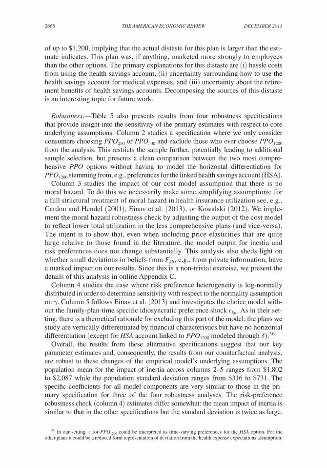
2668 THE AMERICAN ECONOMIC REVIEW dECEMbER 2013
of up to $1,200, implying that the actual distaste for this plan is larger than the esti-mate indicates. This plan was, if anything, marketed more strongly to employees than the other options. The primary explanations for this distaste are (i) hassle costs from using the health savings account, (ii) uncertainty surrounding how to use the health savings account for medical expenses, and (iii) uncertainty about the retire-ment benefits of health savings accounts. Decomposing the sources of this distaste is an interesting topic for future work.
Robustness.—Table 5 also presents results from four robustness specifications that provide insight into the sensitivity of the primary estimates with respect to core underlying assumptions. Column 2 studies a specification where we only consider consumers choosing PP O 250 or PP O 500 and exclude those who ever choose PP O 1200 from the analysis. This restricts the sample further, potentially leading to additional sample selection, but presents a clean comparison between the two most compre-hensive PPO options without having to model the horizontal differentiation for PP O 1200 stemming from, e.g., preferences for the linked health savings account (HSA).
Column 3 studies the impact of our cost model assumption that there is no moral hazard. To do this we necessarily make some simplifying assumptions: for a full structural treatment of moral hazard in health insurance utilization see, e.g., Cardon and Hendel (2001), Einav et al. (2013), or Kowalski (2012). We imple-ment the moral hazard robustness check by adjusting the output of the cost model to reflect lower total utilization in the less comprehensive plans (and vice-versa). The intent is to show that, even when including price elasticities that are quite large relative to those found in the literature, the model output for inertia and risk preferences does not change substantially. This analysis also sheds light on whether small deviations in beliefs from F kjt , e.g., from private information, have a marked impact on our results. Since this is a non-trivial exercise, we present the details of this analysis in online Appendix C.
Column 4 studies the case where risk preference heterogeneity is log-normally distributed in order to determine sensitivity with respect to the normality assumption on γ. Column 5 follows Einav et al. (2013) and investigates the choice model with-out the family-plan-time specific idiosyncratic preference shock ϵ kjt . As in their set-ting, there is a theoretical rationale for excluding this part of the model: the plans we study are vertically differentiated by financial characteristics but have no horizontal differentiation (except for HSA account linked to PP O 1200 modeled through δ ).36
Overall, the results from these alternative specifications suggest that our key parameter estimates and, consequently, the results from our counterfactual analysis, are robust to these changes of the empirical model’s underlying assumptions. The population mean for the impact of inertia across columns 2–5 ranges from $1,802 to $2,087 while the population standard deviation ranges from $316 to $731. The specific coefficients for all model components are very similar to those in the pri-mary specification for three of the four robustness analyses. The risk-preference robustness check (column 4) estimates differ somewhat: the mean impact of inertia is similar to that in the other specifications but the standard deviation is twice as large.
36 In our setting, ϵ for PP O 1200 could be interpreted as time-varying preferences for the HSA option. For the other plans it could be a reduced form representation of deviation from the health expense expectations assumption.

2669handel: adverse selection and inertiavol. 103 no. 7
This reflects the differing estimated coefficients on observable heterogeneity, which are larger in magnitude than in our primary specification. These differences likely arise from the choice implications of the wider tails of risk preferences inherent to the log-normal assumption, which we interpret in the bottom section of Table A-5 in online Appendix E. We now turn to the issue of how reductions to the substantial iner-tia that we find impact consumer choices, adverse selection, and welfare in our setting.
V. Policies that Reduce Inertia: Interaction with Adverse Selection
In this study, consumers enroll in sub-optimal health plans over time, from their perspective, because of inertia. After initially making informed decisions, con-sumers don’t perfectly adjust their choices over time in response to changes to the market environment (e.g., prices) and their own health statuses. In this section, we use the results from the structural consumer choice analysis, together with a model health plan pricing, to investigate the impact of counterfactual policies that improve consumer choices by reducing inertia. This counterfactual analysis is intended to apply broadly to any proposed policies that have the potential to decrease inertia: targeted information provision, premium and benefits change alerts, standardized and simplified insurance plan benefit descriptions, and targeted defaults are four oft-discussed policies, though there are many other relevant ones. Here, we do not differentiate between these policies: to do so would require identification of the vari-ous underlying foundations for inertia. We assume simply that such policies reduce inertia through the mechanism presumed in our structural setup, and discuss why we believe this assumption is relatively innocuous for our purposes. We study the welfare consequences of reduced inertia in both (i) a “naïve” setting where the price of insurance does not change as a consequence of incremental selection and (ii) a “sophisticated” setting where plan prices change to reflect the new risk profile of employees enrolled in the different options.
Model of Reduced Inertia and Plan Pricing.—Formally, our counterfactual analy-sis assumes that the policy being implemented reduces inertia to a fraction Z of the family-specific estimate η k . Thus, Z decreases as the policy more effectively reduces inertia: as Z goes to zero, one could imagine a policy that leads to full re-optimiza-tion in each choice period.37 In this environment, the expected utility of family k for plan j at time t is
U kjt ( P kjt , Z η k , 1 kj, t−1 ) = ∫ 0 ∞ f kjt (OOP)u(OOP, P kjt , Z η k , 1 kj, t−1 )dOOP.
We omit the dependence of utility on the other choice factors modeled in Section III for notational simplicity, though we continue to use all of these factors in the expected utility calculations. Consumers choose the plan j that maximizes their expected util-ity in each period t, subject to the preference estimates from our primary specifica-tion and the assumed lower level of inertia. With endogenous plan pricing, these choices determine health plan costs, which in turn determine health plan premiums,
37 We assume that the policy that reduces inertia is costless, though the analysis could be performed where the policy has a cost that increases as Z declines.

2670 THE AMERICAN ECONOMIC REVIEW dECEMbER 2013
ˆ P kjt . As a result, the plan in which a family enrolls in the environment with reduced inertia depends both on the direct effect of the policy on their choice as well as the indirect effect that it has on premiums resulting from new selection patterns. In the-ory, this collective externality on premiums from reduced inertia could cause either incremental advantageous selection, where the relative price of more comprehensive insurance decreases, or adverse selection, where this relative price increases.
In order to determine the impact of this externality, we model insurance plan pricing. Our model follows the pricing rule used by the firm during the time period studied, and is similar to plan pricing models used in the literature on the welfare consequences of adverse selection across a variety of contexts (see, e.g., Cutler and Reber 1998; or Einav, Finkelstein, and Cullen 2010; or Carlin and Town 2009). The firm we study was self-insured for the PPO options in the choice model, implying that it has full control over the total premiums for each plan option as well as the subsidies employees receive toward those premiums. The total premium paid by employer and employee, T P jt y
, for each plan and year was set as the average plan cost for that plan’s previous year of enrollees, plus an administrative markup, conditional on the dependent coverage tier denoted y :
T P jt y = A C j, t−1 y + L = 1 _
‖ j, t−1 y ‖
Σ k∈ j, t−1 y P P kj, t−1 + L .
Here, j, t−1 y refers to the population of families in plan j at time t − 1 in coverage
tier y. P P kj, t−1 is the total plan paid in medical expenditures conditional on y and j at t − 1. T P jt y
is the amount an employee in dependent category y enrolling in plan j would have to pay each year if they received no health insurance subsidy from the firm. In our setting, the firm subsidizes insurance for each employee as a percentage of the total PP O 1200 premium conditional on the family’s income tier, I k .38 Denote this subsidy S( I k ). Building on these elements, the family-plan-time specific out-of-pocket premium P kjt from the choice model is
P kjt = T P jt y − S( I k )T P PP O 1200 t y
.
For PP O 1200 , P kjt is a fixed percentage of the total premium. For the other two PPO plan options employees additionally pay the full marginal cost of the total premium relative to PP O 1200 . Finally, since P kjt depends on past cost information, we assume that P kj, t 0 equals P kj, t 0 , the actual employee premium contributions set by the firm at t 0 .39 It is important to note that the initial prices at t 0 and the subsequent pricing rule used at the firm are both specific features of the environment that favor incremental adverse selection when inertia is reduced.
Welfare.—We analyze welfare using a certainty equivalent approach that equates the expected utility for each potential health plan option, U kjt , with a certain monetary
38 The subsidy rates for the five income tiers ordered from poorest to wealthiest are 0.97, 0.93, 0.83, 0.71, and 0.64.
39 Presumably, these contributions were set with the expectation that total premiums for each plan would equal average cost, though maintaining this stance is not necessary to assess the impact of inertia reduction policies in our setting, unless the firm would have adjusted P kj, t 0 together with the policies determining Z.
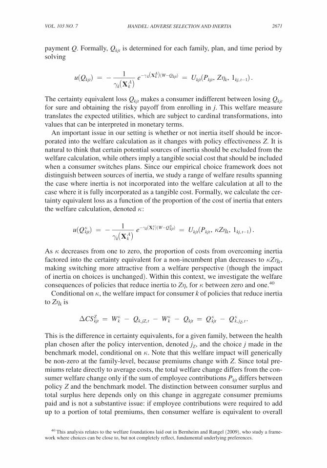
2671handel: adverse selection and inertiavol. 103 no. 7
payment Q. Formally, Q kjt is determined for each family, plan, and time period by solving
u( Q kjt ) = − 1 _ γ k ( X k A )
e − γ k ( X k A ) (W− Q kjt ) = U kjt ( P kjt , Z η k , 1 kj, t−1 ) .
The certainty equivalent loss Q kjt makes a consumer indifferent between losing Q kjt for sure and obtaining the risky payoff from enrolling in j. This welfare measure translates the expected utilities, which are subject to cardinal transformations, into values that can be interpreted in monetary terms.
An important issue in our setting is whether or not inertia itself should be incor-porated into the welfare calculation as it changes with policy effectiveness Z. It is natural to think that certain potential sources of inertia should be excluded from the welfare calculation, while others imply a tangible social cost that should be included when a consumer switches plans. Since our empirical choice framework does not distinguish between sources of inertia, we study a range of welfare results spanning the case where inertia is not incorporated into the welfare calculation at all to the case where it is fully incorporated as a tangible cost. Formally, we calculate the cer-tainty equivalent loss as a function of the proportion of the cost of inertia that enters the welfare calculation, denoted κ :
u( Q kjt κ ) = − 1 _ γ k ( X k A )
e − γ k ( X k A ) (W− Q kjt κ ) = U kjt ( P kjt , κZ η k , 1 kj, t−1 ) .
As κ decreases from one to zero, the proportion of costs from overcoming inertia factored into the certainty equivalent for a non-incumbent plan decreases to κZ η k , making switching more attractive from a welfare perspective (though the impact of inertia on choices is unchanged). Within this context, we investigate the welfare consequences of policies that reduce inertia to Zη, for κ between zero and one.40
Conditional on κ, the welfare impact for consumer k of policies that reduce inertia to Z η k is
ΔC S kjt Z = W k
κ − Q k, jZ, t − W k κ − Q kjt = Q kjt κ − Q k, j Z , t κ .
This is the difference in certainty equivalents, for a given family, between the health plan chosen after the policy intervention, denoted j Z , and the choice j made in the benchmark model, conditional on κ. Note that this welfare impact will generically be non-zero at the family-level, because premiums change with Z. Since total pre-miums relate directly to average costs, the total welfare change differs from the con-sumer welfare change only if the sum of employee contributions P kjt differs between policy Z and the benchmark model. The distinction between consumer surplus and total surplus here depends only on this change in aggregate consumer premiums paid and is not a substantive issue: if employee contributions were required to add up to a portion of total premiums, then consumer welfare is equivalent to overall
40 This analysis relates to the welfare foundations laid out in Bernheim and Rangel (2009), who study a frame-work where choices can be close to, but not completely reflect, fundamental underlying preferences.
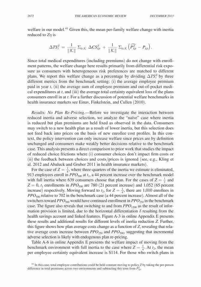
2672 THE AMERICAN ECONOMIC REVIEW dECEMbER 2013
welfare in our model.41 Given this, the mean per-family welfare change with inertia reduced to Zη is
ΔT S t Z = 1 _ ‖ ‖
Σ k∈ ΔC S kjt Z + 1 _
‖ ‖ Σ k∈ ( ˆ P kjt Z
− P kjt ) .
Since total medical expenditures (including premiums) do not change with enroll-ment patterns, the welfare change here results primarily from differential risk expo-sure as consumers with heterogeneous risk preferences are matched to different plans. We report this welfare change as a percentage by dividing ΔT S t Z by three different metrics from the benchmark setting: (i) the average employee premium paid in year t, (ii) the average sum of employee premium and out-of-pocket medi-cal expenditures at t, and (iii) the average total certainty equivalent loss of the plans consumers enroll in at t. For a further discussion of potential welfare benchmarks in health insurance markets see Einav, Finkelstein, and Cullen (2010).
Results: No Plan Re-Pricing.—Before we investigate the interaction between reduced inertia and adverse selection, we analyze the “naïve” case where inertia is reduced but plan premiums are held fixed as observed in the data. Consumers may switch to a new health plan as a result of lower inertia, but this selection does not feed back into prices on the basis of new enrollee cost profiles. In this con-text, the policy intervention can only increase welfare since prices are by definition unchanged and consumers make weakly better decisions relative to the benchmark case. This analysis presents a direct comparison to prior work that studies the impact of reduced choice frictions where (i) consumer choices don’t impact firm costs or (ii) the feedback between choices and costs/prices is ignored (see, e.g., Kling et al. 2012 and Abaluck and Gruber 2011 in health insurance markets).
For the case of Z = 1 _ 4 , where three-quarters of the inertia we estimate is eliminated, 913 employees enroll in PP O 500 at t 1 , a 44 percent increase over the benchmark model with full inertia where 639 consumers choose that plan. For the cases of Z = 1 _ 2 and Z = 0, t 1 enrollments in PP O 500 are 780 (21 percent increase) and 1,052 (65 percent increase) respectively. Moving forward to t 2 , for Z = 1 _ 4 , there are 1,010 enrollees in PP O 500 relative to 702 in the benchmark case (a 44 percent increase). Almost all of the switchers toward PP O 500 would have continued enrollment in PP O 250 in the benchmark case. The figure also reveals that switching to and from PP O 1200 as the result of infor-mation provision is limited, due to the horizontal differentiation δ resulting from the health savings account and linked features. Figure A-3 in online Appendix E presents these results and additional results for different levels of inertia reduction Z. Further, this figure shows how plan average costs change as a function of Z, revealing that rela-tive average costs increase between PP O 250 and PP O 500 , suggesting that incremental adverse selection is likely with endogenous plan re-pricing.
Table A-6 in online Appendix E presents the welfare impact of moving from the benchmark environment with full inertia to the case where Z = 1 _ 4 . At t 2 , the mean per employee certainty equivalent increase is $114. For those who switch plans in
41 In this case, total employee contributions could be held constant moving to policy Z by taking the per-person difference in total premiums across two environments and subtracting this term from P kjt Z
.
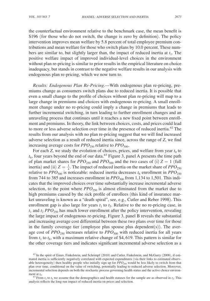
2673handel: adverse selection and inertiavol. 103 no. 7
the counterfactual environment relative to the benchmark case, the mean benefit is $196 (for those who do not switch, the change is zero by definition). The policy intervention improves mean welfare by 5.8 percent of total employee premium con-tributions and mean welfare for those who switch plans by 10.0 percent. These num-bers are similar to, but slightly larger than, the impact of reduced inertia at t 1 . The positive welfare impact of improved individual-level choices in the environment without plan re-pricing is similar to prior results in the empirical literature on choice inadequacy, but stands in contrast to the negative welfare results in our analysis with endogenous plan re-pricing, which we now turn to.
Results: Endogenous Plan Re-Pricing.—With endogenous plan re-pricing, pre-miums change as consumers switch plans due to reduced inertia. It is possible that even a small change to the profile of choices without plan re-pricing will map to a large change in premiums and choices with endogenous re-pricing. A small enroll-ment change under no re-pricing could imply a change in premiums that leads to further incremental switching, in turn leading to further enrollment changes and an unraveling process that continues until it reaches a new fixed point between enroll-ment and premiums. In theory, the link between choices, costs, and prices could lead to more or less adverse selection over time in the presence of reduced inertia.42 The results from our analysis with no plan re-pricing suggest that we will find increased adverse selection as a result of reduced inertia since, across the range of Z, we find increasing average costs for PP O 250 relative to PP O 500 .
For each Z, we study the evolution of choices, prices, and welfare from year t 0 to t 6 , four years beyond the end of our data.43 Figure 3, panel A presents the time path of plan market shares for PP O 250 and PP O 500 and the two cases of (i) Z = 1 (full inertia) and (ii) Z = 1 _ 4 . The impact of reduced inertia on the market share of PP O 250 relative to PP O 500 is noticeable: reduced inertia decreases t 6 enrollment in PP O 250 from 744 to 385 and increases enrollment in PP O 500 from 1,134 to 1,501. This indi-cates that the improved choices over time substantially increase incremental adverse selection, to the point where PP O 250 is almost eliminated from the market due to high premiums caused by the sick profile of enrollees (this kind of insurance mar-ket unraveling is known as a “death spiral”, see, e.g., Cutler and Reber 1998). This enrollment gap is also large for years t 1 to t 5 . Relative to the no re-pricing case, in t 1 and t 2 PP O 250 has much lower enrollment after the policy intervention, revealing the large impact of endogenous re-pricing. Figure 3, panel B reveals the substantial and increasing average cost differential between these two plans over time for those in the family coverage tier (employee plus spouse plus dependent(s)). The aver-age cost of PP O 250 increases relative to PP O 500 with reduced inertia for all years from t 1 to t 6 , with a maximum relative change of $4, 619. This pattern is similar for the other coverage tiers and indicates significant incremental adverse selection as a
42 In the spirit of Einav, Finkelstein, and Schrimpf (2010) and Cutler, Finkelstein, and McGarry (2008), if esti-mated inertia is sufficiently negatively correlated with expected expenditures (via their links to estimated observ-able heterogeneity) then healthy people who initially sign up for PP O 250 would be less likely to switch from that plan over time, conditional on the value of switching, potentially leading to reduced adverse selection. Moreover, incremental selection depends on both the stochastic process governing health status and the active choice environ-ment at t 0 .
43 From t 3 to t 6 we assume that the demographics and health statuses for the sample are as observed in t 2 . This analysis reflects the long-run impact of reduced inertia on prices and selection.
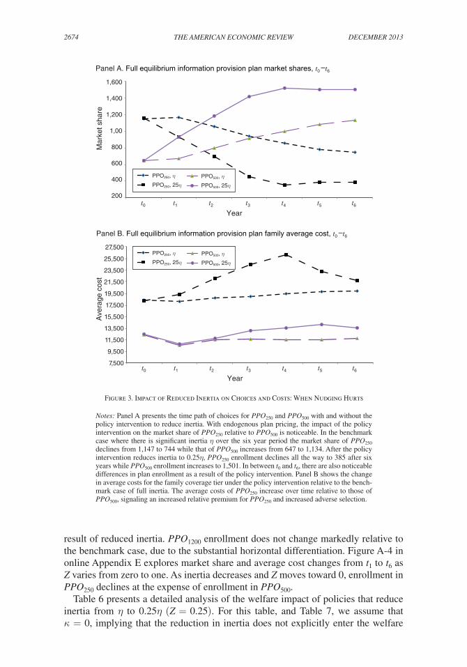
2674 THE AMERICAN ECONOMIC REVIEW dECEMbER 2013
result of reduced inertia. PP O 1200 enrollment does not change markedly relative to the benchmark case, due to the substantial horizontal differentiation. Figure A-4 in online Appendix E explores market share and average cost changes from t 1 to t 6 as Z varies from zero to one. As inertia decreases and Z moves toward 0, enrollment in PP O 250 declines at the expense of enrollment in PP O 500 .
Table 6 presents a detailed analysis of the welfare impact of policies that reduce inertia from η to 0.25η (Z = 0.25). For this table, and Table 7, we assume that κ = 0, implying that the reduction in inertia does not explicitly enter the welfare
Figure 3. Impact of Reduced Inertia on Choices and Costs: When Nudging Hurts
Notes: Panel A presents the time path of choices for PPO250 and PPO500 with and without the policy intervention to reduce inertia. With endogenous plan pricing, the impact of the policy intervention on the market share of PPO250 relative to PPO500 is noticeable. In the benchmark case where there is significant inertia η over the six year period the market share of PPO250 declines from 1,147 to 744 while that of PPO500 increases from 647 to 1,134. After the policy intervention reduces inertia to 0.25η, PPO250 enrollment declines all the way to 385 after six years while PPO500 enrollment increases to 1,501. In between t0 and t6, there are also noticeable differences in plan enrollment as a result of the policy intervention. Panel B shows the change in average costs for the family coverage tier under the policy intervention relative to the bench-mark case of full inertia. The average costs of PPO250 increase over time relative to those of PPO500, signaling an increased relative premium for PPO250 and increased adverse selection.
1,600
1,400
1,200
1,00
800
600
400
200
Mar
ket s
hare
Panel A. Full equilibrium information provision plan market shares, t0 –t6
t0 t1 t2 t3 t4 t5 t6
Year
27,500
25,500
23,500
21,500
19,500
17,500
15,500
13,500
11,500
9,500
7,500
Ave
rage
cos
t
Panel B. Full equilibrium information provision plan family average cost, t0 –t6
t0 t1 t2 t3 t4 t5 t6
Year
PPO250, ηPPO250, 25η
PPO500, ηPPO500, 25η
PPO250, ηPPO250, 25η
PPO500, ηPPO500, 25η

2675handel: adverse selection and inertiavol. 103 no. 7
calculation.44 We calculate the welfare change for the population overall as well as for select groups of interest. For the entire population, the policy that reduces inertia and improves choices has a negative welfare impact in each year and overall. The mean per employee per year certainty equivalent welfare loss is $115, implying an average per person welfare loss of $690 from t 1 to t 6 . This translates to a 7.7 percent loss using average employee premium contributions as a benchmark. Table 6 also reveals that the policy to reduce inertia has substantial distributional consequences. Employees who switch plans as a result of the intervention have an average welfare gain of $186 per employee per year (12.4 percent of average employee premiums).
44 Thus, the welfare impact purely reflects the welfare difference from the choices made and does not incorporate the assumed reduction in inertia as a tangible benefit.
Table 6—Welfare Impact of Reduced Inertia: η to 0.25 η
Plan re-pricing welfare analysisreduced inertia: η to 0.25 η t 1 t 2 t 4 t 6 Avg. t 1 – t 6
Mean Δ TSPopulation −$63 −$104 −$144 −$118 −$115Switcher population percent 51 49 48 53 49Switchers only $86 $175 $ 245 $242 $186Non-switchers only −$205 −$391 −$555 −$432 −$442High expense population percent 10 11 11 11 11High expense $26 $106 $119 $65 $62Non-high expense −$73 −$130 −$177 −$141 −$137Single population percent 47 46 46 46 46Single −$249 −$367 −$414 −$195 −$319W/dependents $99 $124 $89 −$51 $61Low income population percent 40 41 41 41 41Low income −$81 −$218 −$282 −$178 −$200High income −$36 $62 $57 −$30 $0
Welfare change: percent premiums Mean employee premium $1,471 $1,591 $1,455 $1,259 $1,500Welfare change population −4.8 −6.5 −9.9 −9.4 −7.7Welfare change switchers 5.6 11.0 16.9 19.2 12.4Welfare change non-switchers −13.9 −24.6 −38.1 −34.3 −29.4
Welfare change: percent total spendingMean total employee spending $3,755 $4,097 $4,022 $3,862 $4,015Welfare change population −1.7 −2.5 −3.6 −3.06 −2.9Welfare change switchers 2.3 4.3 6.1 6.3 4.6Welfare change non-switchers −5.5 −9.5 −13.8 −11.2 −11.0
Welfare change: percent ‖ CEQ ‖ LossMean total ‖ CEQ ‖ Loss $5,888 $6,264 $6,207 $6,065 $6,190Welfare change population −1.1 −1.7 −2.3 −2.0 −1.9Welfare change switchers 1.5 2.8 4.0 4.0 3.0Welfare change non-switchers −3.5 −6.2 −8.9 −7.1 −7.1
Notes: This table presents the welfare results of the endogenous insurance pricing policy counterfactual for the case where inertia is reduced from η to 0.25 η. We present the change in the mean per employee per year certainty equiv-alent moving from the simulation with full inertia to the one with reduced inertia. In addition to studying the effect of the policy on efficiency, we study the distributional effects based on four categorizations (i) “switchers”, or peo-ple who are in a different plan at time t under the policy intervention than without it; (ii) an indicator of whether or not the family has high health costs relative to its coverage tier; (iii) whether an employee is single or covers depen-dents; and (iv) whether an employee has high or low income. The three welfare metrics we present take the ratio of the change in certainty equivalent with respect to (i) total employee premiums, (ii) total employee spending, and (iii) the absolute value of the certainty equivalent loss.
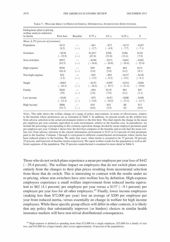
2676 THE AMERICAN ECONOMIC REVIEW dECEMbER 2013
Those who do not switch plans experience a mean per employee per year loss of $442 (−29.4 percent). The welfare impact on employees that do not switch plans comes entirely from the changes to their plan prices resulting from incremental selection from those that do switch. This is interesting to contrast with the results under no re-pricing, where non-switchers have zero welfare loss by definition. High-expense employees experience a small welfare improvement from reduced inertia equiva-lent to $62 (4.1 percent) per employee per year versus a $137 (−9.1 percent) per employee per year loss for all other employees.45 Finally, lower income employees (making less than $72,000 per year) lose an average of $200 per employee per year from reduced inertia, versus essentially no change in welfare for high income employees. While these specific group effects will differ in other contexts, it is likely that any policy that substantially improves (or hinders) choices in similar health insurance markets will have non-trivial distributional consequences.
45 High-expense is defined as spending more than $15,000 for a single employee, $25,000 for a family of size two, and $32,000 for a larger family (this covers approximately 10 percent of the population).
Table 7—Welfare Impact of Reduced Inertia: Differential Intervention Effectiveness
Endogenous plan re-pricing welfare analysis reduction in inertia First-best Baseline 0.75 η 0.5 η 0.25 η 0
Mean Δ TS (percent of premiums)Population $123 — −$41 −$73 −$115 −$107
(8.2) (—) (−2.7) (−4.9) (−7.7) (−7.1)
Switchers −$538 — $1,017 $766 $186 $118 (−35.9) (—) (67.8) (51.0) (12.4) (7.9)
Non-switchers $953 — −$249 −$371 −$442 −$382 (63.5) (—) (−16.6) (−24.8) (−29.4) (−25.4)
High expense $936 — $38 $84 $62 $121 (62.4) (—) (2.6) (5.6) (4.2) (8.1)
Non-high expense $22 — −$52 −$93 −$137 −$136 (1.5) (—) (−3.5) (−6.2) (−9.2) (−9.1)
Single −$683 — −$153 −$295 −$319 −$286 (−45.5) (—) (−10.2) (−19.7) (−21.2) (−19.0)
Family $826 — −$54 $119 $61 $47 (55) (—) (3.6) (7.9) (4.1) (3.1)
Low income −$349 — −$75 −$153 −$200 −$190 (−23.3) (—) (−5.0) (−10.2) (−13.3) (−12.7)
High income $806 — $10 $43 $0 $13 (53.7) (—) (0.6) (2.9) (0) (0.9)
Notes: This table shows the welfare change of a range of policy interventions, in terms of effectiveness, relative to the baseline where preferences are as estimated in Table 5. In addition, we present results on the welfare loss from adverse selection in the actual environment relative to the first-best. The chart reports the change in the mean per employee per year certainty equivalent in each environment, relative to the baseline case. In parentheses, we include the percentage corresponding to this certainty equivalent change divided by mean employee premiums paid per employee per year. Column 1 shows how the first-best compares to the baseline and reveals that the mean wel-fare loss from adverse selection in the current information environment is $123 or 8.2 percent of total premiums paid in the baseline. Columns 3 through 6 correspond to different counterfactual environments where inertia has been reduced relative to the baseline. We study four cases, when inertia is assumed to be 75 percent, 50 percent, 25 percent, and 0 percent of baseline inertia respectively. We report welfare results for the population as well as dif-ferent segments of the population. The 25 percent counterfactual is examined in more detail in Table 6.
2677handel: adverse selection and inertiavol. 103 no. 7
Table 7 broadens the analysis and considers differing levels of effectiveness for policies that reduce inertia, including the cases of Z equal to 0.75, 0.5, 0.25, and 0. We also study the welfare loss of adverse selection in our observed setting relative to the conditional first-best outcome, which for our model and environment is all employees enrolled in PP O 250 in every time period. The table presents the average per employee per year certainty equivalent change for each of these counterfactual scenarios relative to the baseline (analogous to the last column in Table 6), with per-centage changes reported relative to average employee premium contributions. The welfare loss from adverse selection in the baseline relative to the first best is $123 (−8.2 percent) per employee per year.46 This welfare loss increases as Z declines from 1 to 0.25. For Z equal to 0.75, 0.5, and 0.25 the incremental losses relative to our baseline are $41 (−2.7 percent), $73 (−4.9 percent), and $115 (−7.7 percent) respectively. For Z = 0, this loss is $107 (−7.1 percent), a slightly smaller loss than that when Z = 0.25.47 The table also presents the welfare impact for select popula-tion groups for different levels of inertia. As in Table 6, there are substantial dis-tributional consequences from policies that reduce inertia (and from achieving the conditional first-best). Notably, employees who switch plans as a result of reduced inertia have a substantial welfare gain equivalent to $1,017 (68 percent) per person when Z = 0.75, which decreases to $118 (7.9 percent) when Z = 0. For those who don’t switch, the welfare loss ranges from $249 (−16.6 percent) in the former case to $382 (−25.4 percent) in the latter.
Table 8 expands the analysis further to allow for the possibility that some proportion of estimated, and subsequently reduced, inertia be incorporated as a tangible cost into the welfare calculation when consumers switch plans. The top panel studies the maxi-mum average inertia cost incurred from switching plans for different Z, reflecting the scenario where inertia occurs purely due to tangible switching or search costs. Over t 1 to t 6 the mean per employee per year maximum inertial cost incurred from switching is $185 for the baseline case, $188 for Z = 0.75, and $142 and $83 for Z = 0.5 and Z = 0.25 respectively. These figures reflect the product of the number of switchers and the maximum direct inertial cost incurred in these counter factual environments.
The bottom panel of Table 8 gives the welfare impact for the range of policies described by Z, similarly to Table 7, as a function of κ, the proportion of inertia that represents a tangible cost when a consumer switches plans. Results are presented for κ equal to zero (no tangible cost when overcoming inertia), 0.25, 0.5, and 1 (purely tangible costs). The results for κ = 0 restate the results from Table 7. When κ = 0.25, the welfare change caused by the policy intervention is $90 (−6.0 percent) for Z = 0.25, compared to the $115 loss when κ = 0. In the extreme case when all inertia represents a tangible and welfare relevant cost (κ = 1) the Z = 0.25 policy leads to a $13 (−0.9 percent) loss. More broadly, the table reveals that the impact of including a higher proportion of inertia in the welfare calculation is larger
46 This can be compared directly to the numbers found in the literature on the welfare consequences of adverse selection. Cutler and Reber (1998) find that the welfare loss from adverse selection in their environment is between 2– 4 percent of total baseline spending. In our setting, when re-normalized by this metric, we find a welfare loss of 2.9 percent, right in the middle of this range. Recent work by Carlin and Town (2009); Bundorf, Levin, and Mahoney (2012); Einav, Finkelstein, and Cullen (2010); and Einav et al. (2013) find results that are in this ballpark in a variety of empirical settings.
47 This non-monotonicity of the welfare loss in Z near 0 arises because, when inertia is entirely removed, pre-miums and enrollment oscillate toward a stable equilibrium rather than move monotonically to that steady state.

2678 THE AMERICAN ECONOMIC REVIEW dECEMbER 2013
the more inertia is reduced by the intervention. For example, the welfare impact of Z = 0.75 relative to the baseline is close to constant as a function of κ, while the more effective Z = 0.25 intervention has a wider range of potential welfare impacts as κ varies. Notably, the welfare impact is negative across the range of κ for all Z except Z = 0, suggesting that reduced inertia will lead to increased adverse selec-tion and lower welfare in our setting regardless of the stance taken on κ.48
It is important to emphasize that the negative welfare impact from reduced iner-tia that we find is specific to our setting on multiple dimensions. First, we study a specific population with specific preferences and health risk profiles: the direction of the welfare impact could be reversed with a different population in the same market environment. Second, the market environment that we study is specific. This is reflected, for example, by the plans available, initial plan prices at t 0 , and the subsidy rule. The direction of the welfare impact could be reversed with the same population in a different market environment. The main generalizable implication is that the interaction between adverse selection and inertia can have substantial, and potentially surprising, welfare implications in a given empirical setting.
Finally, we note that while the empirical framework specifies inertia as a direct cost (similar to a tangible search or switching cost), we believe that alternative choice model specifications would yield similar conclusions for both the extent of inertia and its interaction with adverse selection. Consider an alternative framework with two stages. In the first stage a consumer decides whether or not to search and re-optimize,
48 For Z = 0, the welfare impact of the intervention is negative for κ of 0, 0.25, and 0.5 but positive for κ = 1. Thus, when overcoming inertia purely represents a tangible cost, and inertia is reduced entirely by the policy, wel-fare increases. In this case, there is still increased adverse selection from the policy, but the positive welfare effect from the reduction in inertial costs paid outweighs the negative impact of adverse selection.
Table 8—Different Welfare Treatments of Inertia
Endogenous plan re-pricingWelfare treatment of inertia
η 0.75 η 0.5 η 0.25 η 0
Avg. t 1 – t 6 Inertia cost/ switcher 1,963 1,489 988 493 0Switcher % 9 13 14 17 20
Avg. inertia pop. 185 188 142 83 0
Welfare impact η 0.75 η 0.5 η 0.25 η 0κ = 0 Welfare relevant inertia 0 0 0 0 0
Δ TS (% premiums) — −$41 (−2.7) −$73 (−4.9) −$115 (−7.7) −$107 (−7.1)
κ = 0.25 Welfare relevant inertia 46 47 36 21 0Δ TS (% premiums) — −$42 (−2.8) −$63 (−4.2) −$90 (−6.0) −$61 (−4.1)
κ = 0.5 Welfare relevant inertia 93 94 71 42 0Δ TS (% premiums) — −$42 (−2.8) −$51 (−3.4) −$64 (−4.3) −$14 (−0.9)
κ = 1 Welfare relevant inertia 185 188 142 83 0Δ TS (% premiums) — −$44 (−2.9) −$30 (−2.0) −$13 (−0.9) −$78 (5.2)
Notes: Table 8 expands the welfare analysis to account for the possibility that some proportion of estimated, and subsequently reduced, inertia should be included in the welfare analysis. Tables 6 and 7 present results conditional on κ = 0 (overcoming inertia is not welfare relevant cost) while this table presents results across the range of κ from 0 to 1 (overcoming inertia is purely a direct and welfare relevant cost). The top panel of this table studies the profile of maximum incurred tangible costs of inertia for different Z from t1 to t6, while the bottom panel assesses the welfare impact of these interventions as a function of κ. The table reveals that, for almost all combinations of κ and Z, there is a negative welfare impact from reduced inertia and better consumer decisions.
2679handel: adverse selection and inertiavol. 103 no. 7
based on beliefs about the market environment and a cost of re-optimization, while in the second stage the consumer actively chooses a plan conditional on deciding to re-optimize in stage one. The η estimated in our framework would translate into the cost of re-optimization and beliefs about the market environment in the proposed alternative framework, leading to a similar degree of overall choice persistence. In the counterfactual setting where inertia is entirely reduced, both models predict that all consumers re-optimize perfectly in every time period.49 Since non-inertial preferences are identified based on choices made in the active choice year, t 0 , estimated active preferences will be similar in both models and preferences under fully reduced inertia will be similar in both models. As a result, the environment with markedly reduced inertia would have similarly increased adverse selection, regardless of the exact micro-foundations for inertia. It is important to note that, for interim cases between full inertia and no inertia these models could have different predictions for who switches and who doesn’t. The two-stage model predicts that anyone who re-optimizes and has a positive benefit from switching will do so, while, for the primary model in the paper, only those who prefer an alternative plan by Zη more than the incumbent plan will switch.50 See online Appendix D for an expanded discussion of these issues.
VI. Conclusion
There is a general consensus in the policy debate on the design and regulation of health insurance markets that helping consumers make the best plan choices pos-sible is unequivocally the right course of action, regardless of the specifics of the environment. The Affordable Care Act (ACA) mandates clear and simple informa-tion provision for plans offered through state-run exchanges while there has been a similar emphasis in the employer-sponsored insurance market on providing con-sumers increased plan options and the capabilities to choose between them (see, e.g., Kaiser Family Foundation 2011). In both public and private settings, market regulators have worked to create and implement policies and tools to help consum-ers make better choices including (i) standardized and simplified benefits descrip-tions, (ii) premium and benefits changes alerts, (iii) targeted plan recommendations, and (iv) targeted default options. All of these options have the potential to improve individual-level plan enrollments in both active choice and inertial environments.
This paper highlights (i) that inertia can be substantial in health insurance markets and (ii) that efforts to improve choices in health insurance markets with consumer inertia should take into account the potential impact on incremental adverse selec-tion. We cleanly identify the extent of inertia by leveraging a panel dataset where all consumers must make an active plan choice from a new menu of health plans in one specific year but must deal with inertia in other years. Several model-free preliminary analyses reveal that inertia has a substantial impact on health plan enroll-ment as the choice environment evolves over time. We estimate a choice model of
49 In the alternative model, instead of re-optimizing some of the time, consumers always re-optimize when inertia is fully reduced. This is the same as the case when Z = 0 in our primary model and there is no utility wedge between incumbent and non-incumbent plans.
50 Given the similar predictions for full inertia and no inertia in both models, and the specifics of our environ-ment, it is highly likely that partially reduced inertia would still result in increased adverse selection in the alterna-tive two-stage model, as it does in our primary specification.
2680 THE AMERICAN ECONOMIC REVIEW dECEMbER 2013
consumer decision-making under uncertainty to quantify inertia, ex ante health risk distributions, and risk preferences that yields clear evidence of large and hetero-geneous inertia. We use this model to study the impact of counterfactual policies that reduce inertia, without differentiating between specific policies. While reducing inertia increases welfare in the naïve setting where health plan prices are held fixed, in the setting where health plan premiums adjust as enrollees switch plans reduced inertia leads to incremental adverse selection and a welfare loss. When inertia is reduced by three-quarters, this incremental welfare loss effectively doubles the wel-fare loss from adverse selection in the observed environment (8.2 percent of con-sumer premiums). Though these results are specific to our setting, they illustrate that the interaction between inertia and adverse selection can be quite important, and that policies to improve consumer choices in health insurance markets should consider the potential for incremental risk-based plan selection.
The impact of reduced inertia on incremental adverse selection also depends on insurance market pricing policies such as (i) subsidies and (ii) insurer-level risk adjustment. The lump-sum subsidies and average cost-plus pricing in our environment are features of many employer-sponsored and public insurance markets. Lump-sum subsidies are usually motivated by the desire to encourage consumers to internalize price signals and choose plans more efficiently. However, in the absence of effective insurer-level risk-adjustment transfers, when consumers face the full marginal price of incremental insurance, in general, a smaller and more expensive profile of con-sumers will select comprehensive insurance as its relative price increases, leading to greater adverse selection (Cutler and Reber 1998).51 Subsidy policies that pay some proportion of the cost of incremental coverage will generally mitigate adverse selec-tion to some extent. Insurer-level risk-adjustment transfers, discussed in Cutler and Reber (1998) and incorporated into the ACA exchanges, can also mitigate adverse selection when layered on top of average cost pricing and lump sum subsidies. With insurer-level risk adjustment, the market regulator arranges transfers between insur-ers to reflect differences in the ex ante (or ex post) risk profile of the consumers these plans enroll. Ideally, plans set premiums that reflect consumer valuations and net out expected health expenditures, eliminating adverse selection based on ex ante observ-ables. In our setting, incorporating risk-adjustment transfers into premium setting would bound the welfare impact from reduced inertia between our results and the first-best. The degree to which welfare would improve toward the first-best depends both on (i) the effectiveness of the risk-adjustment scheme and (ii) the distribution of population preferences. One implication of this work is that policies to reduce iner-tia should be considered in light of how effective insurer-level risk-adjustment is. If risk-adjustment is relatively ineffective, as shown in Brown et al. (2011) for Medicare Advantage, then reduced inertia could have significant implications for adverse selec-tion. As risk-adjustment becomes more effective, potential adverse selection is con-strained, leaving only the positive effects of improving individual-level choices.
Improved consumer choices will also have implications for firm behavior in insur-ance markets. Reduced inertia could have desirable effects not considered here, such as
51 This is true as long as additional dimensions of preference heterogeneity are not highly negatively correlated with expected health expenditures (see, e.g., Einav, Finkelstein, and Schrimpf 2010 or Cutler, Finkelstein, and McGarry 2008).
2681handel: adverse selection and inertiavol. 103 no. 7
enhancing the efficiency of product offerings through increased competition. In a mar-ket environment, these benefits could outweigh any losses from potentially increased adverse selection. Additionally, even with substantial regulation, firms competing in a free market would likely incorporate consumer inertia into pricing decisions. While prior work reveals that the implications of this kind of dynamic pricing can be quite subtle even without considering adverse selection (see, e.g., Farrell and Klemperer 2007 or Viard 2007), we believe that this is an intriguing area for future work.
REFERENCES
Abaluck, Jason, and Jonathan Gruber. 2011. “Choice Inconsistencies among the Elderly: Evidence from Plan Choice in the Medicare Part D Program.” American Economic Review 101 (4): 1180–1210.
Akerlof, George A. 1970. “The Market for ‘Lemons’: Quality Uncertainty and the Market Mecha-nism.” Quarterly Journal of Economics 84 (3): 488–500.
Bernheim, B. Douglas, and Antonio Rangel. 2009. “Beyond Revealed Preference: Choice-Theoretic Foundations for Behavioral Welfare Economics.” Quarterly Journal of Economics 124 (1): 51–104.
Brown, Jason, Mark Duggan, Ilyana Kuziemko, and William Woolston. 2011. “How Does Risk Selec-tion Respond to Risk Adjustment? Evidence From The Medicare Advantage Program.” National Bureau of Economic Research Working Paper 16977.
Bundorf, M. Kate, Jonathan Levin, and Neale Mahoney. 2012. “Pricing and Welfare in Health Plan Choice.” American Economic Review 102 (7): 3214–48.
Cardon, James H., and Igal Hendel. 2001. “Asymmetric Information in Health Insurance: Evidence from the National Medical Expenditure Survey.” RAND Journal of Economics 32 (3): 408–27.
Carlin, Caroline, and Robert Town. 2009. “Adverse Selection, Welfare and the Optimal Pricing of Employer Sponsored Health Plans.” Unpublished.
Chandra, Amitabh, Jonathan Gruber, and Robin McKnight. 2010. “Patient Cost-Sharing and Hospi-talization Offsets in the Elderly.” American Economic Review 100 (1): 193–213.
Chiappori, Pierre-Andre, and Bernard Salanie. 2000. “Testing for Asymmetric Information in Insur-ance Markets.” Journal of Political Economy 108 (1): 56–78.
Cohen, Alma, and Liran Einav. 2007. “Estimating Risk Preferences from Deductible Choice.” Ameri-can Economic Review 97 (3): 745–88.
Crawford, Gregory S., Nicola Tosini, and Keith Waehrer. 2011. “The Impact of ‘Rollover’ Contracts on Switching Costs in the UK Voice Market: Evidence from Disaggregate Customer Billing Data.” CEPR Discussion Paper DP8693.
Cutler, David M., Amy Finkelstein, and Kathleen McGarry. 2008. “Preference Heterogeneity and Insurance Markets: Explaining a Puzzle of Insurance.” American Economic Review 98 (2): 157–62.
Cutler, David, Bryan Lincoln, and Richard Zeckhauser. 2010. “Selection Stories: Understanding Movement across Health Plans.” Journal of Health Economics 29 (6): 821–38.
Cutler, David M., and Sarah J. Reber. 1998. “Paying for Health Insurance: The Trade-Off between Competition and Adverse Selection.” Quarterly Journal of Economics 113 (2): 433–66.
DeNavas-Walt, Carmen, Bernadette D. Proctor, and Jessica C. Smith. 2010. Income, Poverty, and Health Insurance Coverage in the United States: 2009. U.S. Census Bureau, Current Population Reports, P60-238. Washington, DC: U.S. Government Printing Office.
Dube, Jean-Pierre, Gunter J. Hitsch, and Peter E. Rossi. 2009. “Do Switching Costs Make Markets Less Competitive?” Journal of Marketing Research 46 (4): 435–45.
Dube, Jean-Pierre, Gunter J. Hitsch, and Peter E. Rossi. 2010. “State Dependence and Alternative Explanations for Consumer Inertia.” RAND Journal of Economics 41 (3): 417–45.
Dube, Jean-Pierre, Gunter J. Hitsch, Peter E. Rossi, and Maria Ana Vitorino. 2008. “Category Pricing with State-Dependent Utility.” Marketing Science 27 (3): 417–29.
Einav, Liran, Amy Finkelstein, and Mark R. Cullen. 2010. “Estimating Welfare in Insurance Markets Using Variation in Prices.” Quarterly Journal of Economics 125 (3): 877–921.
Einav, Liran, Amy Finkelstein, and Jonathan Levin. 2010. “Beyond Testing: Empirical Models of Insurance Markets.” Annual Review of Economics 2 (1): 311–36.
Einav, Liran, Amy Finkelstein, Stephen P. Ryan, Paul Schrimpf, and Mark R. Cullen. 2013. “Selection on Moral Hazard in Health Insurance.” American Economic Review 103 (1): 178–219.
Einav, Liran, Amy Finkelstein, and Paul Schrimpf. 2010. “Optimal Mandates and the Welfare Cost of Asymmetric Information: Evidence from the U.K. Annuity Market.” Econometrica 78 (3): 1031–92.

2682 THE AMERICAN ECONOMIC REVIEW dECEMbER 2013
Ericson, Keith M. Marzilli. 2012. “Market Design When Firms Interact with Inertial Consumers: Evi-dence from Medicare Part D.” Unpublished.
Fang, Hanming, Michael P. Keane, and Dan Silverman. 2008. “Sources of Advantageous Selection: Evidence from the Medigap Insurance Market.” Journal of Political Economy 116 (2): 303–50.
Farrell, Joseph, and Paul Klemperer. 2007. “Coordination and Lock-In: Competition with Switching Costs and Network Effects.” In Handbook of Industrial Organization, Vol. 3, edited by M. Arm-strong and R. Porter, 1967–2072. Amsterdam: Elsevier B. V.
Finkelstein, Amy, and James Poterba. 2006. “Testing for Adverse Selection with ‘Unused Observ-ables’.” National Bureau of Economic Research Working Paper 12112.
Goettler, Ronald L., and Karen Clay. 2011. “Tariff Choice with Consumer Learning and Switching Costs.” Journal of Marketing Research, 48 (4): 633–52.
Handel, Benjamin R. 2013. “Adverse Selection and Inertia in Health Insurance Markets: When Nudg-ing Hurts: Dataset.” American Economic Review. http://dx.doi.org/10.1257/aer.103.7.2643.
Kaiser Family Foundation. 2010a. “Employer Health Benefits: 2010 Annual Survey.” http://ehbs.kff.org/pdf/2010/8085.pdf (accessed August 2011).
Kaiser Family Foundation. 2011. “Focus on Health Reform: Summary of New Health Reform Law.” http://kaiserfamilyfoundation.files.worldpress.com/2011/04/8061-021.pdf (accessed August 2011).
Kling, Jeffrey R., Sendhil Mullainathan, Eldar Shafir, Lee C. Vermeulen, and Marian V. Wrobel. 2012. “Comparison Friction: Experimental Evidence from Medicare Drug Plans.” Quarterly Journal of Economics 127 (1): 199–235.
Kowalski, Amanda E. 2012. “Estimating the Tradeoff Between Risk Protection and Moral Hazard with a Nonlinear Budget Set Model of Health Insurance.” National Bureau of Economic Research Work-ing Paper 18108.
Madrian, Brigitte C., and Dennis F. Shea. 2001. “The Power of Suggestion: Inertia in 401(k) Participa-tion and Savings Behavior.” Quarterly Journal of Economics 116 (4): 1149–87.
McManus, Margaret A., Stephen Berman, Thomas McInerny, and Suk-fong Tang. 2006. “Weighing the Risks of Consumer-Driven Health Plans for Families.” Pediatrics 117 (4): 1420–24.
Reed, Mary, Vicki Fung, and Mary Price et al. 2009. “High-Deductible Health Insurance Plans: Efforts to Sharpen a Blunt Instrument.” Health Affairs 28 (4): 1145–53.
Rothschild, Michael, and Joseph E. Stiglitz. 1976. “Equilibrium in Competitive Insurance Markets: An Essay on the Economics of Imperfect Information.” Quarterly Journal of Economics 90 (4): 630–49.
Shum, Matthew. 2004. “Does Advertising Overcome Brand Loyalty? Evidence from the Breakfast-Cereals Market.” Journal of Economics and Management Strategy 13 (2): 241–72.
Strombom, Bruce A., Thomas C. Buchmueller, and Paul J. Feldstein. 2002. “Switching Costs, Price Sensitivity and Health Plan Choice.” Journal of Health Economics 21 (1): 89–116.
Thaler, Richard H., and Cass R. Sunstein. 2008. Nudge: Improving Decisions about Health, Wealth, and Happiness. New Haven: Yale University Press.
Train, Kenneth E. 2009. Discrete Choice Methods with Simulation, 2nd ed. New York: Cambridge University Press.
Viard, V. Brian. 2007. “Do Switching Costs Make Markets More or Less Competitive? The Case of 800-Number Portability.” RAND Journal of Economics 38 (1): 146–63.