1

(Preliminary and Incomplete)

Adverse Selection and Subsidies: Evidence from

Non-group Health Insurance Markets

Rajeev Cherukupalli*

Columbia University

rc2063@columbia.edu

October 15 2008

Abstract

Adverse selection is a problem in health insurance markets when premiums do not fully reflect individuals' risks. Premium subsidies in such markets can potentially reduce adverse selection by encouraging low-risk individuals to participate and seek greater insurance coverage. I test this premise using Current Population Survey and income tax data in the context of two concurrent and unrelated policy changes that have affected state non-group markets. Adverse selection was induced in the subset of state non-group markets which adopted community rating, a set of premium restrictions that increased the price of coverage for younger, healthier individuals. Over the same period, a series of federal tax law changes reduced the effective after-tax premiums for the self-employed, providing a subsidy to a subset of participants in non-group markets over and above that induced by the tax system in the crosssection. In line with the theory, I find that healthier individuals in the segment of the market affected by rating restrictions were more likely to purchase insurance if they received a larger effective subsidy.

* I thank Sherry Glied, Dan O’Flaherty and Wojeciech Kopczuk for their guidance and support, and Amitabh Chandra and participants at student colloquia at Columbia University for helpful comments. This paper is as yet incomplete, and all errors are mine.

2

I. Introduction and Literature

Adverse selection is a problem in markets with asymmetric information. Insurance markets typify

this situation, and insurers tend to offer menus of contracts with different combinations of premiums and

coverage to separate buyers on the basis of their risk. If buyers in an insurance market are offered a

uniform premium, the set of individuals who find it worth buying coverage will tend to have above-

average risks. The problem is compounded in health insurance markets, when insurers are restricted in

their ability to use different dimensions of risk in arriving at the premium they charge a customer.

This delinking of health risk from the price that people pay to be insured against those risks is a

feature of both group insurance offered by employers and of insurance purchased in some non-group

markets. In an employer sponsored plan, a sicker and a healthier employee might pay the same price

despite their very different expected health expenses. Analogously, in some non-group markets, insurers

are barred from using risk-related characteristics like age and gender in the price of the plans they offer.

When voluntary health insurance purchase is combined with such pricing restrictions, the concern is that

the composition of buyers in the market can shift to sicker individuals. Adverse selection can cause

insurers to raise premiums higher, further reducing avenues for coverage for the larger population.

Adverse selection imposes a negative externality in that the inability to use private information in

pricing insurance contracts spills over into under-insurance. A natural question to ask is whether a subsidy

can help reduce or eliminate adverse selection. This paper examines the question of whether tax subsidies

mitigate adverse selection by exploiting two concurrent and unrelated policy changes that have interacted

to affect state-level non-group insurance markets in the United States since the early 1990s. While one

policy induced selection in a set of states that adopted it, the other policy changed the magnitude of

subsidies available to a sub-segment of the market over time.

The state policy variation that potentially induced selection is community rating, implemented by

states that sought to ensure that high-cost individuals were not priced out of insurance. Community rating

restrictions have the effect of reducing insurers’ ability to separate consumers based on health risks.

While the intent of community rating is to make access to care more equitable, its viability depends on

lower risks staying in the insurance pool. Different sources, both descriptive and in the empirical

literature suggest that community rating was associated with increased premiums, and with reduced

enrollment and exit by insurers (Wachenheim and Leida, 2007; LoSasso and Lurie, 2007).

3

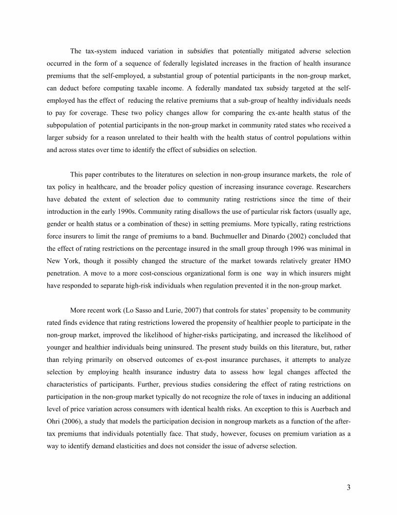
The tax-system induced variation in subsidies that potentially mitigated adverse selection

occurred in the form of a sequence of federally legislated increases in the fraction of health insurance

premiums that the self-employed, a substantial group of potential participants in the non-group market,

can deduct before computing taxable income. A federally mandated tax subsidy targeted at the self-

employed has the effect of reducing the relative premiums that a sub-group of healthy individuals needs

to pay for coverage. These two policy changes allow for comparing the ex-ante health status of the

subpopulation of potential participants in the non-group market in community rated states who received a

larger subsidy for a reason unrelated to their health with the health status of control populations within

and across states over time to identify the effect of subsidies on selection.

This paper contributes to the literatures on selection in non-group insurance markets, the role of

tax policy in healthcare, and the broader policy question of increasing insurance coverage. Researchers

have debated the extent of selection due to community rating restrictions since the time of their

introduction in the early 1990s. Community rating disallows the use of particular risk factors (usually age,

gender or health status or a combination of these) in setting premiums. More typically, rating restrictions

force insurers to limit the range of premiums to a band. Buchmueller and Dinardo (2002) concluded that

the effect of rating restrictions on the percentage insured in the small group through 1996 was minimal in

New York, though it possibly changed the structure of the market towards relatively greater HMO

penetration. A move to a more cost-conscious organizational form is one way in which insurers might

have responded to separate high-risk individuals when regulation prevented it in the non-group market.

More recent work (Lo Sasso and Lurie, 2007) that controls for states’ propensity to be community

rated finds evidence that rating restrictions lowered the propensity of healthier people to participate in the

non-group market, improved the likelihood of higher-risks participating, and increased the likelihood of

younger and healthier individuals being uninsured. The present study builds on this literature, but, rather

than relying primarily on observed outcomes of ex-post insurance purchases, it attempts to analyze

selection by employing health insurance industry data to assess how legal changes affected the

characteristics of participants. Further, previous studies considering the effect of rating restrictions on

participation in the non-group market typically do not recognize the role of taxes in inducing an additional

level of price variation across consumers with identical health risks. An exception to this is Auerbach and

Ohri (2006), a study that models the participation decision in nongroup markets as a function of the after-

tax premiums that individuals potentially face. That study, however, focuses on premium variation as a

way to identify demand elasticities and does not consider the issue of adverse selection.

4

The relation between tax policy and health insurance coverage has been the subject of continued

research in economics and public policy. Income taxation interacts with individuals’ insurance purchase

decisions at different levels—employers’ contributions to insurance are not subject to tax, individuals can

often purchase coverage out of pre-tax dollars, and medical expenses above a threshold can be deducted

to reduce overall tax liability. Given the pervasiveness of this interaction, studies are typically concerned

with two aspects of the influence of the tax system on health: the effectiveness of the tax subsidies in

improving coverage (Gruber and Poterba, 1994, Finkelstein, 2002), and the moral hazard induced by the

reduction in the effective price of medical care (Gruber and Washington, 2004). The present study

considers a less researched dimension of the tax system in the spirit of Cutler and Zeckhauser (1998),

namely the extent to which subsidies might act as a risk adjusment to restrict the degree of adverse

selection in situations where premiums are imperfectly related to purchasers’ health risks.

Cutler and Zeckhauser (1998) represents a smaller body of literature that examines the the effect

of subsidies on mitigating selection, typically in employer sponsored groups. Their study examined the

effect of the suspension of an equal contribution rule in a university’s health plan offerings. The step,

analogous to the withdrawal of an untargeted subsidy, encouraged low-risk individuals to withdraw from

more comprehensive and expensive plans. This sort of unraveling of plans is at the heart of the tradeoff

between pooling individuals of different risks to achieve a viable level of cross-subsidizing and curbing

incentives to use excessive and expensive care . Selden and Gray (2002) study the effect of a subsidy on

the Federal Employees Health Benefits Program, where the presence of both a national plan with fixed

premiums and a set of several local plans with varying premiums made it optimal for healthier employees

to select into the lowest cost plan they faced to avoid subsidizing high-cost employees. The FEHBP has a

nominally set maximum allowable premium subsidy, resulting in variation in the implied real local-level

subsidy. Selden and Gray find that older individuals selected into plans with higher premiums, but this

apparent adverse selection was slightly dampened by the larger effective subsidy that younger participants

received.

Ketsche (2004) uses cross-sectional data from the National Medical Expenditure Survey, 1987, to

ask whether receiving a larger subsidy on account of having a higher marginal tax rate increases the

participation of workers who are less healthy, or who have families with members in poorer health. The

present study is closest in its approach to Ketsche’s paper, with the advantage of having better

identification than was available in the cross-sectional setting that Ketsche uses. On the side of selection,

the variation in the present study that induces healthier people to be less likely to be insured is cross-state

differences in regulation of the non-group and small-group markets. Ketsche’s study does not have a

5

similar exogenous source driving the incentive for healthier people to drop coverage, and is confined to

using state income tax deciles rather than the precise imputed state tax to identify variation in subsidies.

On the side of variation in price that might mitigate adverse selection, the present study investigates state

insurance markets over more than a decade. Over this period the subsidy changes for a sub-population of

buyers were increases in allowable tax deductions of a magnitude ranging from 25 to 100 per cent of the

premium paid. These operate over and above the differences in effective after-tax subsidy brought about

by individuals being placed at different income levels and having different marginal taxes.

A more general interpretation of this paper is in the context of externalities in insurance markets.

Adverse selection is a negative externality that causes a deviation from the first best outcome of optimal

insurance for all health risks, since low risk individuals willing to purchase insurance are induced to

obtain suboptimal coverage or to drop coverage. A subsidy to such individuals, whether through the tax

system as in this instance, or though other conceivable forms, can improve welfare in contexts that make

insurance markets imperfect. Einav, Finkelstein and Cullen (2008), for example, suggest that adverse

selection is associated with an efficiency cost of 3 per cent relative to what obtains with efficient pricing.

How efficiently a tax subsidy serves to correct selection depends on the costs the subsidy imposes relative

to the benefits of reduced selection. The present study attempts to measure some of these potential

benefits in a context where the source of the externality and the subsidy affecting this externality are

identified relatively cleanly.

The paper proceeds as follows. Section II briefly examines the theoretical reasons for how a

subsidy can mitigate selection in a standard Rothschild-Stiglitz (1979) framework. Section III outlines the

empirical strategy and the two contexts, community rating and tax-policy induced variation in premiums

that this study exploits in identifying the effect of subsidies on adverse selection. Section IV describes the

data used in the analysis and presents evidence pointing to the differential effect of subsidies on selection

in community rated and non- community rated states. Section V develops the empirical models used and

discusses the results on selection and whether the tax system reduced selection, and Section VI concludes.

II. Theoretical Framework

Figure 1 depicts the standard Rothschild-Stiglitz (R-S) equilibrium in a health insurance market

in the absence of any subsidy. The horizontal axis represent individuals’ wealth in the event of their

facing no health loss, while the vertical axis represents wealth in the event that individuals face a health

loss. The 45-degree line OO´ represents equal wealth combinations in each state, and therefore first-best

6

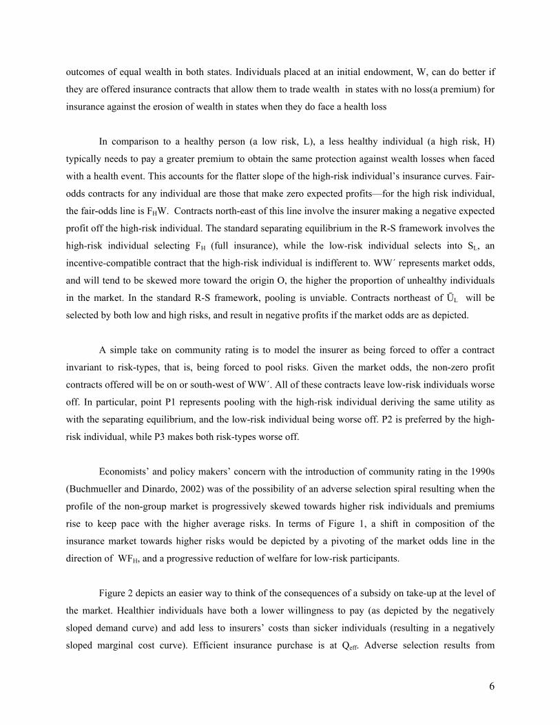
outcomes of equal wealth in both states. Individuals placed at an initial endowment, W, can do better if

they are offered insurance contracts that allow them to trade wealth in states with no loss(a premium) for

insurance against the erosion of wealth in states when they do face a health loss

In comparison to a healthy person (a low risk, L), a less healthy individual (a high risk, H)

typically needs to pay a greater premium to obtain the same protection against wealth losses when faced

with a health event. This accounts for the flatter slope of the high-risk individual’s insurance curves. Fair-

odds contracts for any individual are those that make zero expected profits—for the high risk individual,

the fair-odds line is FHW. Contracts north-east of this line involve the insurer making a negative expected

profit off the high-risk individual. The standard separating equilibrium in the R-S framework involves the

high-risk individual selecting FH (full insurance), while the low-risk individual selects into SL, an

incentive-compatible contract that the high-risk individual is indifferent to. WW´ represents market odds,

and will tend to be skewed more toward the origin O, the higher the proportion of unhealthy individuals

in the market. In the standard R-S framework, pooling is unviable. Contracts northeast of ŪL will be

selected by both low and high risks, and result in negative profits if the market odds are as depicted.

A simple take on community rating is to model the insurer as being forced to offer a contract

invariant to risk-types, that is, being forced to pool risks. Given the market odds, the non-zero profit

contracts offered will be on or south-west of WW´. All of these contracts leave low-risk individuals worse

off. In particular, point P1 represents pooling with the high-risk individual deriving the same utility as

with the separating equilibrium, and the low-risk individual being worse off. P2 is preferred by the high-

risk individual, while P3 makes both risk-types worse off.

Economists’ and policy makers’ concern with the introduction of community rating in the 1990s

(Buchmueller and Dinardo, 2002) was of the possibility of an adverse selection spiral resulting when the

profile of the non-group market is progressively skewed towards higher risk individuals and premiums

rise to keep pace with the higher average risks. In terms of Figure 1, a shift in composition of the

insurance market towards higher risks would be depicted by a pivoting of the market odds line in the

direction of WFH, and a progressive reduction of welfare for low-risk participants.

Figure 2 depicts an easier way to think of the consequences of a subsidy on take-up at the level of

the market. Healthier individuals have both a lower willingness to pay (as depicted by the negatively

sloped demand curve) and add less to insurers’ costs than sicker individuals (resulting in a negatively

sloped marginal cost curve). Efficient insurance purchase is at Qeff. Adverse selection results from

7

insurers having to charge a uniform price, at the point where average costs equal willingness to pay in the

figure. In a competitive equilibrium, the mass of individuals covered—or, more generally, the quantify of

coverage offered in the market—is Q1, resulting in an efficiency loss equal to the area ABC. A subsidy,

represented by an outward shift of the demand curve, can potential offset some of this efficiency loss,

while increasing coverage to Q3. An untargeted subsidy carries its own efficiency loss (the area ADE),

but to the extent that a subsidy scheme can be designed to mimic the marginal cost curve, the lower these

losses will tend to be.

III. Empirical Strategy

Subsidies can influence selection along two margins—who chooses to purchase insurance, and

how much coverage they demand. This paper focuses on the former decision. An ideal experiment to test

if subsidies reduce the extent of selection would involve offering two insurance contracts with identical

coverage but different subsidies to two populations with an identical distribution of health risks. A

measure of the effect of the subsidy is the extent to which take-up in the subsidized population exceeds

that in the unsubsidized population. A second measure is the generosity of coverage individuals select,

but that cannot be captured in the data.

In the absence of the ideal experiment, I investigate adverse selection in the context of two policy

induced variations affecting the non-group (and small-group) insurance market in the United States. In

line with related empirical work, I first compare the observable risk profile of individuals in the market

for nongroup insurance in community rated states with those in unregulated states to verify whether

restricting the range of premiums induces higher risk individuals to participate, and/or reduces the

purchase of insurance by lower risk individuals. Thereafter, I test if receiving a larger subsidy has the

effect of inducing lower risk individuals in community rated states to purchase insurance. The empirical

strategy is thus to develop variants of the following estimation equation

— (1)

CR in the above is an indicator of whether a state is community rated (or of years since the enforcement

of rating regulations). Affected is an indicator for potential purchasers of nongroup insurance affected by

the rating restrictions, and healthy is one of different proxies for individuals’ health risks. The coefficients

εγγγ

γγγβ

effects year effects state6subsidy*healthy * affected* CR5healthy * affected* CR 4subsidy*affected*CR

3healthy * affected* CR affected* CR CR X ed)Prob(insur

++++++

+++= 21

8

of particular interest are 3γ and 5γ . If the model is correctly identified, a negative 3γ indicates that the

community rating tends to draw less healthy participants, while a positive 5γ indicates if and to what

extent a subsidy restores the balance towards healthier participants.

Community rating restrictions

The non-group market in the US accounts for about 7 per cent of all insurance purchases and is

largely unregulated. Given the predominance of employer-sponsored insurance, the non-group market is

typically a residual market with a large variation in the number of insurers and types of contracts on offer.

Beginning in the early 1990s, a some states began to implement regulations to make insurance in the non-

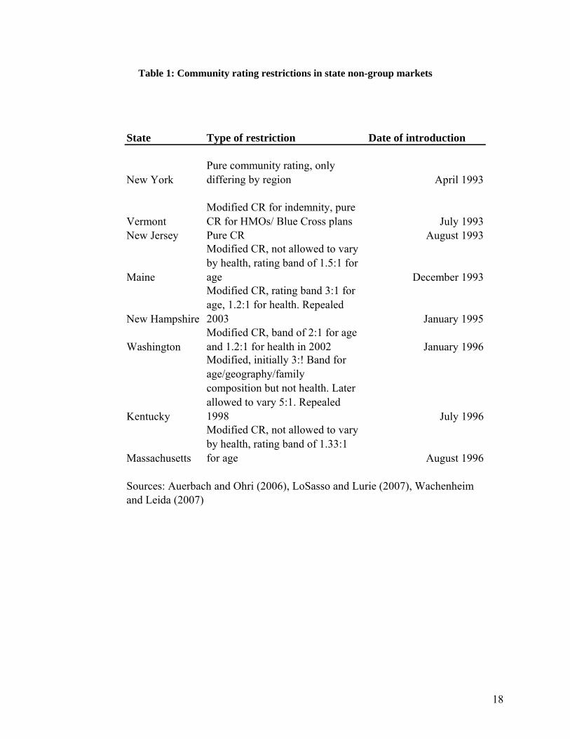
group market more affordable to high-riks individuals. Table 1 outlines these restrictions. New York is

the one state with pure community rating: while premium variation is allowed in benefit plan design,

family type and geographic regions, premiums are not allowed to vary by age or health for any given plan.

Other states typically prescribe a band within which premiums can vary—a 3:1 age band, for instance,

would allow a 60 year old male to be charged a premium that is at most three times what a 20 year old

male is charged, even though, by some estimates, the expected health expenses.

Whether community rating changes participation and risk composition in non-group markets is an

empirical question. There are a few factors that can attenuate any effect. The first is the presence of

institutional factors that pre-empt rating restrictions. While New York’s was an instance of pure

community rating, the official rule largely followed the existing voluntary rating practice of the largest

insurance carrier in the combined non-group and small group market. Second, there are several ways in

which insurers might respond to circumvent rating restrictions. States with weaker restrictions, for

instance, have both a larger menu of plans offered and higher rates of rejection of applicants by their

dominant insurance carriers (Turnbull and Kane, 2005). Observed changes in participation in community

rated states are thus necessarily reduced-form effects of purchase decisions of individuals conditional on

the menu of plans offered.

A larger set of states adopted restrictions in the small-group market in the same period of the

study, and the shift to community rating restrictions was associated with decline in coverage for low-risk

individuals and a passing on of the costs of increased premiums to workers (Simon, 2005). I also consider

these states in the empirical model of the decision of those affected by rating restrictions to be privately

insured.

9

Tax price variation

The income tax system induces variation in the after-tax price that individuals pay for insurance.

Two individuals with the same health risks and offered the same insurance contract face different after-

tax prices depending on their incomes, deductions and state of residence.The marginal tax price of

insurance is a measure of the after-tax cost of an additional dollar of premium purchased. To the extent

that insurance purchases are made out of after-tax incomes, the price of additional coverage decreases in

the marginal tax rate.

Given a schedule of premiums and individuals’ insurance purchase decisions, identifiying the

effect of price subsidies is confounded by the fact that unobservables might drive both the decision to be

covered and the tendency to select contracts with higher premiums. The advantage to using tax prices in

considering the effect of subsidies on selection is that federal tax policy induces exogenous variation in

the price of insurance. There are, however, caveats to using tax prices as a method of identifying the

effect of prices (Feenberg, 1987; Andreoni, 2006). What matters for the economic analysis of decisions

on the margin is the additional dollar of insurance, or the last dollar tax price. The last dollar tax price,

however, is a function of premiums paid—a taxpayer with a large premium potentially faces a higher

effective tax price. A solution is to use the first dollar price, a price computed as if individuals had no

insurance and were contemplating paying a premium of one dollar.

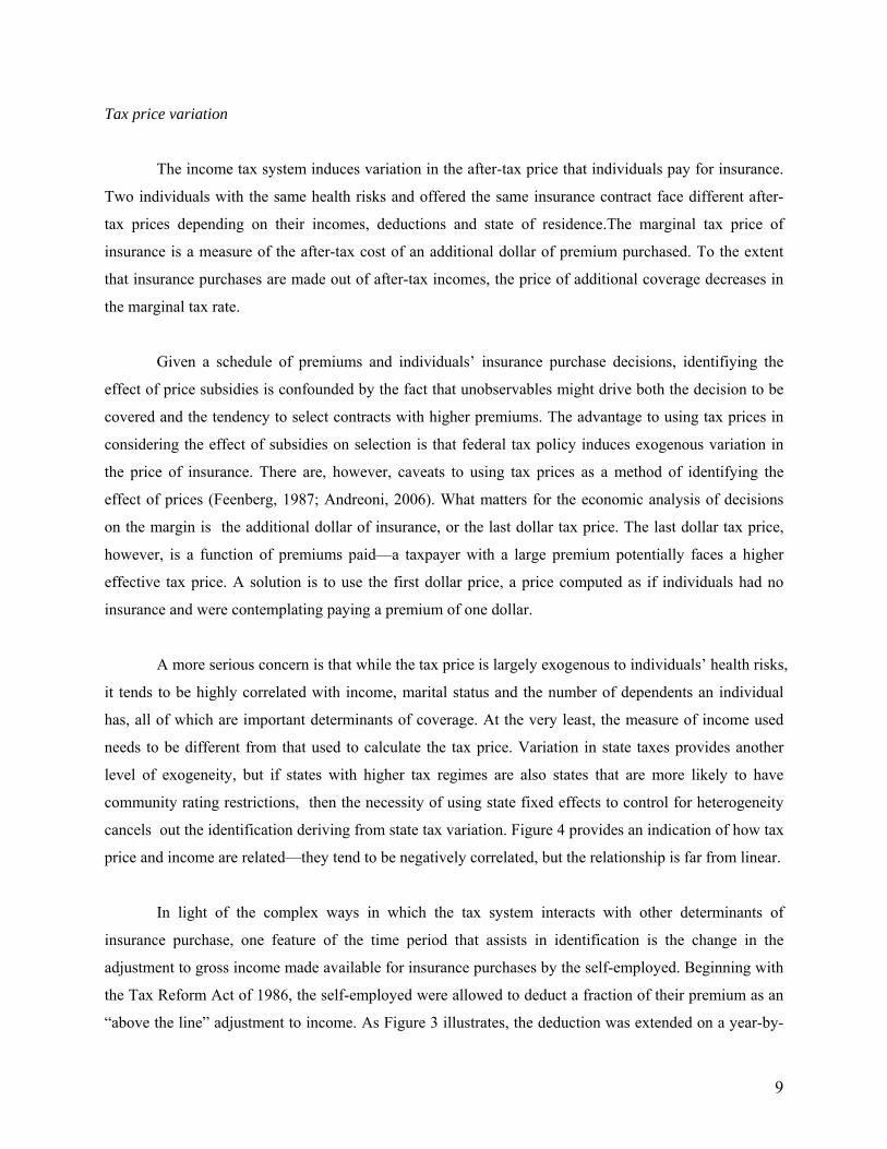
A more serious concern is that while the tax price is largely exogenous to individuals’ health risks,

it tends to be highly correlated with income, marital status and the number of dependents an individual

has, all of which are important determinants of coverage. At the very least, the measure of income used

needs to be different from that used to calculate the tax price. Variation in state taxes provides another

level of exogeneity, but if states with higher tax regimes are also states that are more likely to have

community rating restrictions, then the necessity of using state fixed effects to control for heterogeneity

cancels out the identification deriving from state tax variation. Figure 4 provides an indication of how tax

price and income are related—they tend to be negatively correlated, but the relationship is far from linear.

In light of the complex ways in which the tax system interacts with other determinants of

insurance purchase, one feature of the time period that assists in identification is the change in the

adjustment to gross income made available for insurance purchases by the self-employed. Beginning with

the Tax Reform Act of 1986, the self-employed were allowed to deduct a fraction of their premium as an

“above the line” adjustment to income. As Figure 3 illustrates, the deduction was extended on a year-by-

10

year basis over the decade, and was increased periodically from 25 per cent through 1995 to 100 per cent

by 2003. Self-employed taxpayers constitute between 8 and 21 percent percent of taxpayers in state non-

group markets and 14 percent nationwide. This is relevant to identifying the effect of subsidies on

selection through sources other than cross-sectional variation, since the self-employed are a subgroup of

the potential market for nongroup insurance that received a subsidy that others did not receive. Panel A in

Figure 5 displays how this variation plays out along the income distribution in community rated states—

over time, the effective tax price declined for the self-employed at all levels of the income distribution.

Panel B suggests that there are variations in insurance purchase beyond that observed across the income

distribution, though insurance purchase for the self-employed tends to be noisier.

IV. Data

I use March Current Population Survey data for 1990-2005 for the purpose of the estimation

exercise. The advantages of the CPS are the ability to identify good proxies for income, to retain large

sample sizes for estimating effects on subgroups such as the selfemployed in a subset of states, and, in

contrast to the SIPP, the ability to identify firm size easily, firm size being an important determinant of

the likelihood of insurance offer and purchase. These advantages come with well-recognized

disadvantages, including the cross-sectional nature of the data, and the absence of detailed measures of

health insurance plan attributes and individuals’ health status. Further, when estimating empirical models

that use self-reported health status as a control, I am restricted to periods after 1995 when the health status

questions were introduced in the CPS.

The unit of observation is the individual tax payer in the age group 19 to 64. I drop individuals

covered by Medicare, Medicaid or other forms of publicly funded and military coverage since the

insurance purchase calculus is considerably different for these groups. I compute tax prices using NBER’s

TAXSIM software to obtain marginal tax rates for individuals in the sample. For employees of firms, the

tax price is computed as

(1-tfed-tstate-tFICA/2) if wage/salary employee (1- θ(tfed+ tstate)) if self-employed

where tfed, tstateA and tFICA represent the federal, state and social security marginal tax rates and θ is the

fraction of the insurance premium that can be deducted as an adjustment to income by the self-employed

(0.25 through 1995 and a 100 per cent from 2003).

11

Table 2 displays summary statistics for the start and end period considered. Aside of family

income, there appears little variation in means of the variables, though there is a 20 per cent decline in

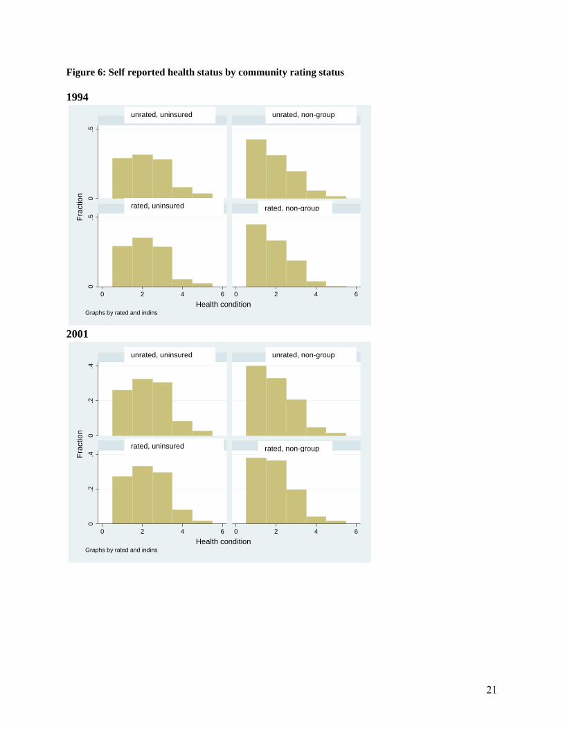
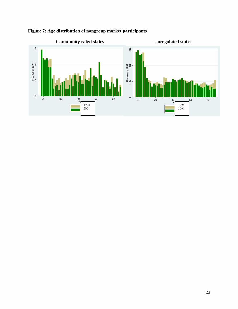
participation in the nongroup market in community rated states. Figures 6 through 8 offer a better picture

of some of the transitions in the rated and unregulated states over the period. Figure 6 indicates a small

increase in the fraction of non-group insured people in community rated states reporting poor health status.

Figure 7 indicates that there might have been a transition in age profile in the nongroup market in

community rated states, with the distribution becoming more bimodal than previously. In comparison, the

unregulated states have a stable distribution of age profiles.

Age and self-reported health status are important dimensions of health risk, but are obviously

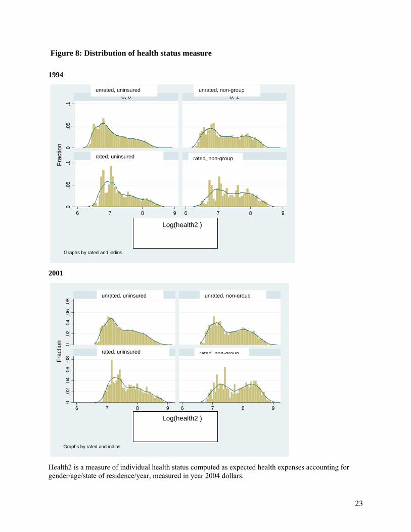
imperfect proxies. To get at a better approximation of the distribution of health risks in states, I construct

two measures of individuals expected health status, Healthrisk and Healthrisk2, building on Auerbach

and Ohri (2006). The measure is a lower bound estimate of health expenses that any individual can expect

to have and is constructed as follows: Using a nation-wide insurer’s schedule of premiums for plans

offered in Florida (an unregulated state), I compute age- and gender-specific annual premiums for every

individual in any part of the country. Adding the deductible gives an estimate of expected health expenses

for individuals as if they were all residing in Florida in 2004. To convert this measure into the state- and

year-specific expenses they can expect, I use the league tables of state- and year-specific per capita

personal health care expenditures from the Center of Medicare and Medicaid Services (CMS) to construct

an index of expenses over time and states of residence relative to Florida in 2004. Figure 8 thus captures

the transition of health risks as the result of changes in age and gender composition in rated and unrated

states, and suggests that rated states might have seen a concentration at both the upper and the lower ends

of the distribution. Healthrisk2 is a measure that further adjusts Healthrisk1 upwards for individuals with

self-reported health on the basis of MEPS data on how the expected health expenses of individuals with

different self-reported health status relates to those in excellent health. While necessarily arbitrary, these

measures are intended to capture the fact that age, gender and self-reported health interact in predictable

ways and are used by insurers in forming an idea of the risk composition of the markets they sell in.

V. Models and results

V. 1 Evidence from Subpopulations on Selection

As a first pass at understanding if community rating affects coverage, I estimate models of the following

form:

12

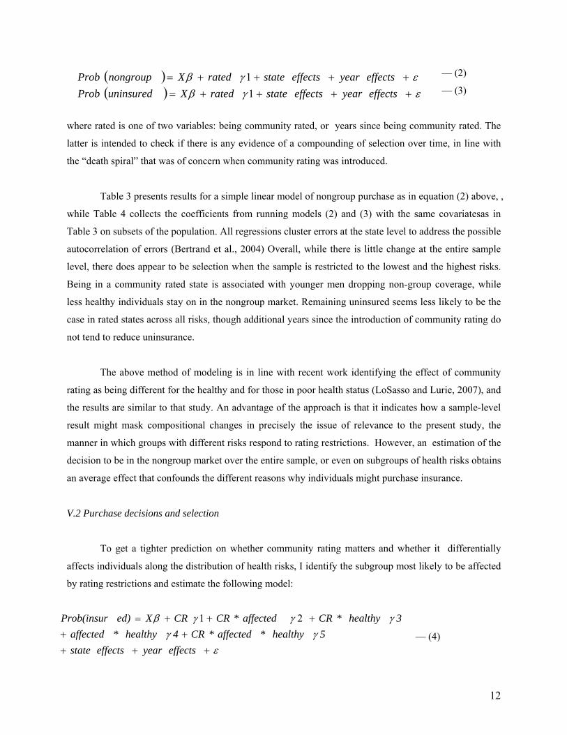
— (2)

— (3)

where rated is one of two variables: being community rated, or years since being community rated. The

latter is intended to check if there is any evidence of a compounding of selection over time, in line with

the “death spiral” that was of concern when community rating was introduced.

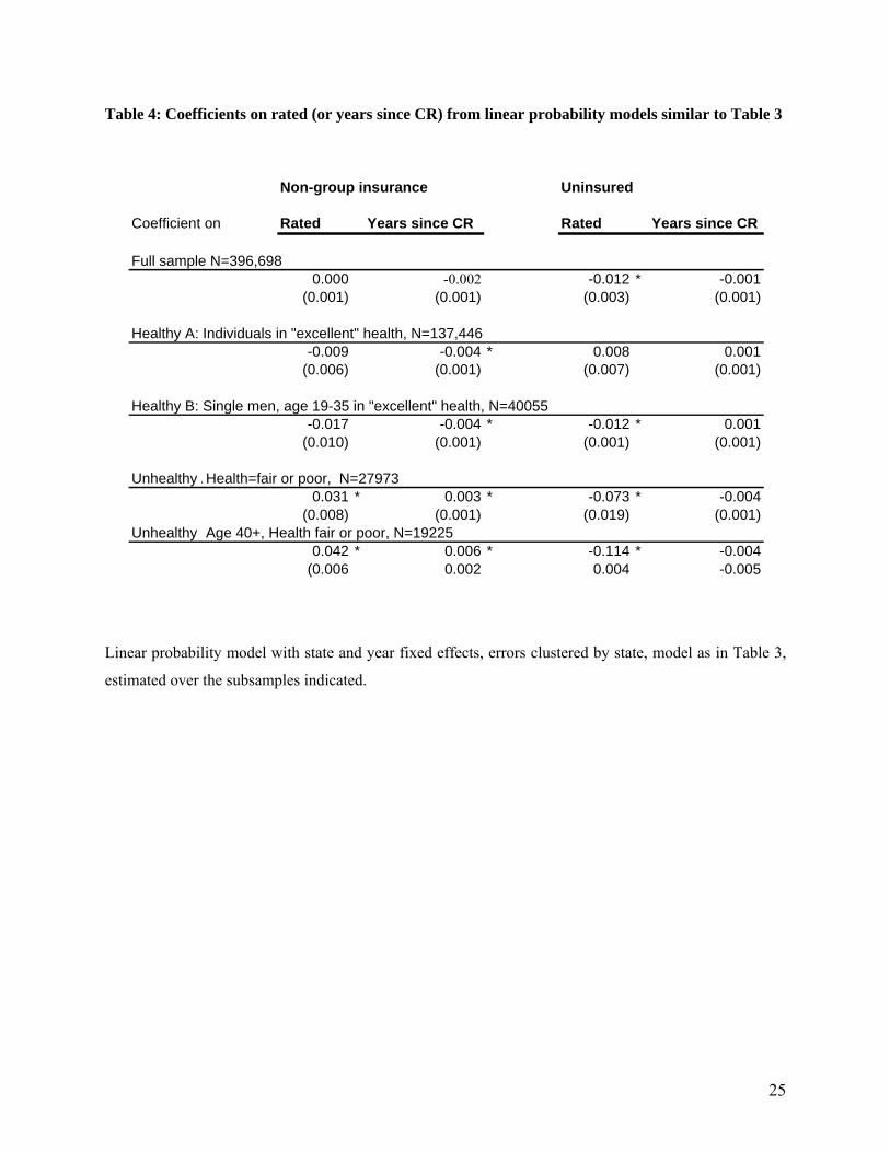
Table 3 presents results for a simple linear model of nongroup purchase as in equation (2) above, ,

while Table 4 collects the coefficients from running models (2) and (3) with the same covariatesas in

Table 3 on subsets of the population. All regressions cluster errors at the state level to address the possible

autocorrelation of errors (Bertrand et al., 2004) Overall, while there is little change at the entire sample

level, there does appear to be selection when the sample is restricted to the lowest and the highest risks.

Being in a community rated state is associated with younger men dropping non-group coverage, while

less healthy individuals stay on in the nongroup market. Remaining uninsured seems less likely to be the

case in rated states across all risks, though additional years since the introduction of community rating do

not tend to reduce uninsurance.

The above method of modeling is in line with recent work identifying the effect of community

rating as being different for the healthy and for those in poor health status (LoSasso and Lurie, 2007), and

the results are similar to that study. An advantage of the approach is that it indicates how a sample-level

result might mask compositional changes in precisely the issue of relevance to the present study, the

manner in which groups with different risks respond to rating restrictions. However, an estimation of the

decision to be in the nongroup market over the entire sample, or even on subgroups of health risks obtains

an average effect that confounds the different reasons why individuals might purchase insurance.

V.2 Purchase decisions and selection

To get a tighter prediction on whether community rating matters and whether it differentially

affects individuals along the distribution of health risks, I identify the subgroup most likely to be affected

by rating restrictions and estimate the following model:

— (4)

( )( ) εγβ

εγβ effects year effects state rated X uninsuredProb effects year effects state rated X nongroupProb

++++=++++=

11

εγγ

γγγβ

effects year effects state5healthy * affected* CR4healthy * affected

3healthy * CR affected* CR CR X ed)Prob(insur

+++++

+++= 21

13

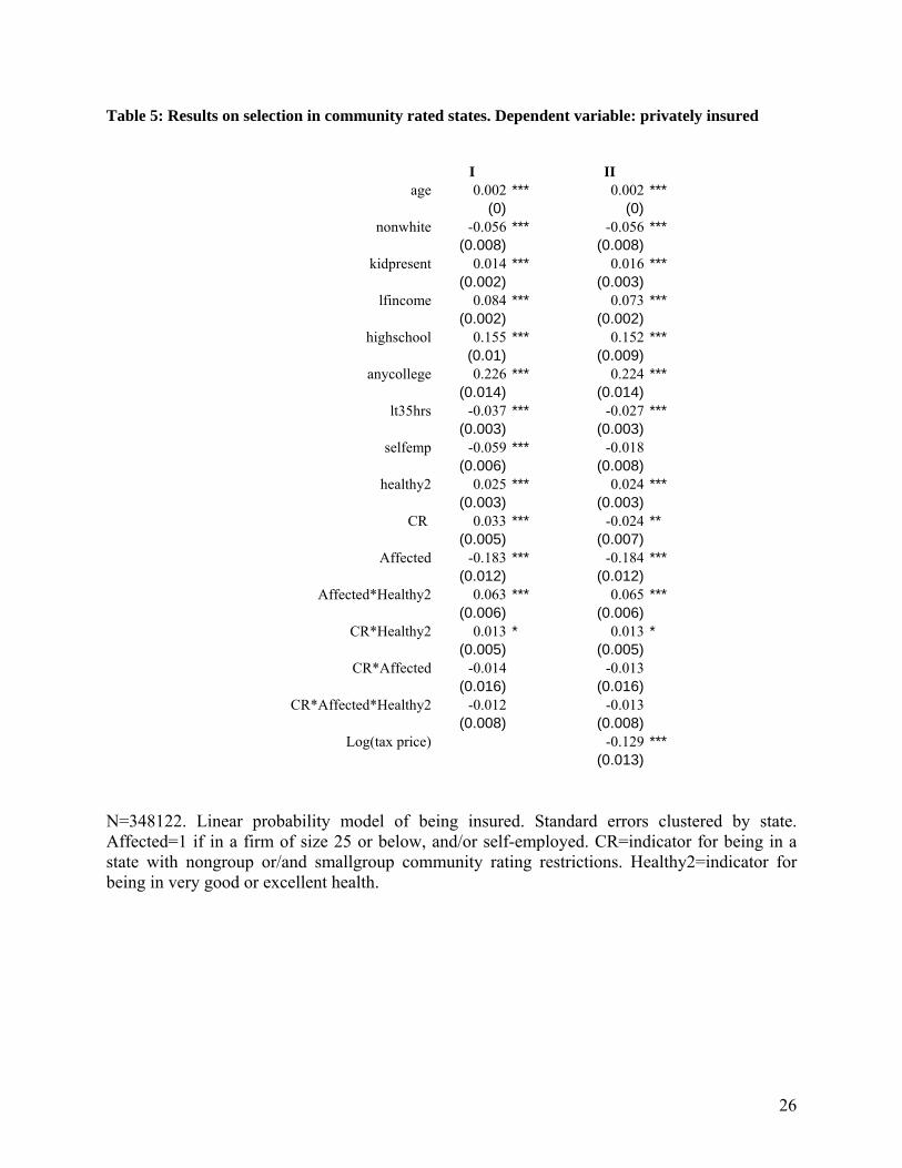
In the above, affected is an indicator for whether a person is in a firm of size less than 25, and/or

self-employed. CR is an indicator for having nongroup or small-group community rating restrictions and

healthy is an indicator for being in excellent or very good health. I later experiment with the more

continuous definition of health risk described in Section IV above . Table 5 indicates that those affected

in community rated states are slightly less likely to purchase insurance, the sign on the differential effect

for the healthiest for these individuals is as expected (the healthiest in the affected group less likely to

participate in rated states) but is not individually significant. Log(tax price) in Column II of Table 5

carries the expected sign—larger subsidies are associated with lower participation.

V.2 Effect of Subsidies

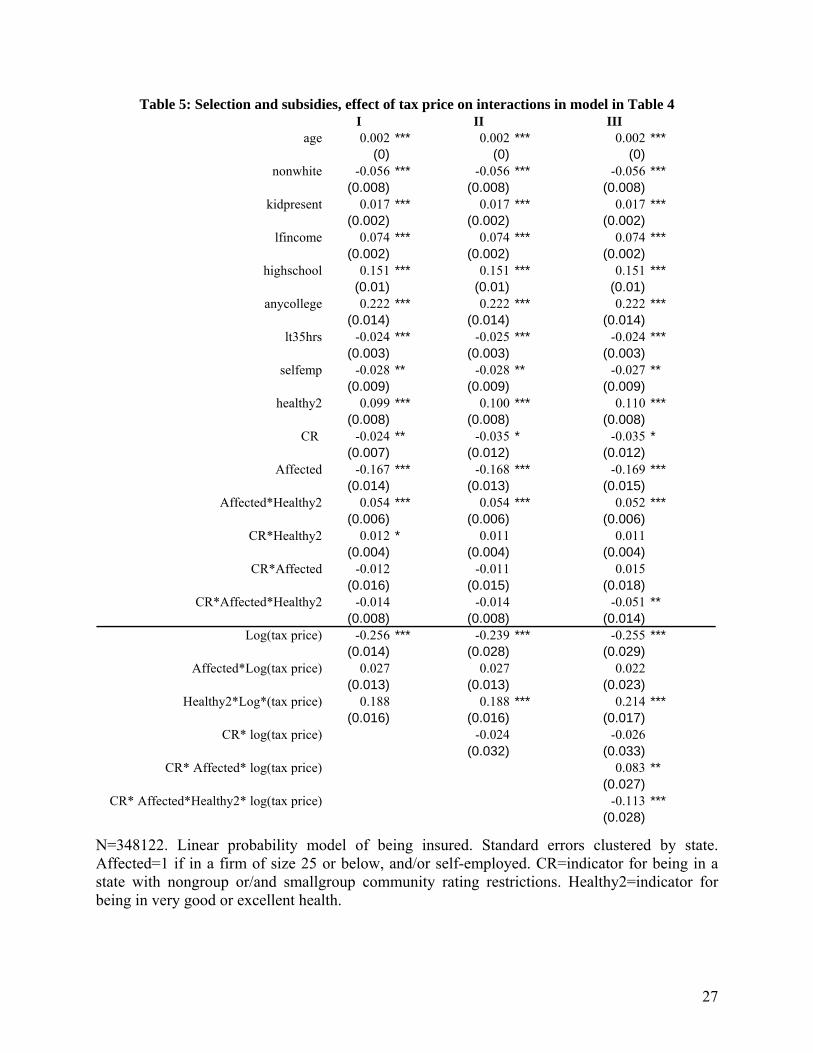
Modifying equation (4) above to incorporate the variation in tax prices yields estimation

equations of the form outlined in section III

— (5)

While Model (5) appears complex, it differs from (4) only in the addition of the variable

log(taxprice) and the interaction of log(taxprice) with the variables that identify a differential participation

by healthier individuals subjected to adverse selection. The main coefficient of interest is now 11γ , the

differential effect of being subsidized for healthier individuals in the affected subgroup in community

rated states. A higher tax price for healthier individuals is lowers their probability of purchasing insurance.

This is consistent with a subsidy being differentially beneficial in retaining healthier individuals in the

presence of adverse seleciton.

VI.3 Results with a continuous measure of health status

I now restrict the sample further to assess if the above model holds when the population

considered closer to those affected by nongroup market regulations (rather than both nongroup and small

εγ

γγγγγ

γγγγγβ

effects year effects state11ce)log(taxpri*healthy* affected* CR

10ce)log(taxpri*healthy* affected ce)log(taxpri*healthy * CR ce)log(taxpri* affected* CR 7price) log(tax*CR6 price) log(tax

5healthy * affected* CR4y health* affected 3healthy * CR affected* CR CR X ed)Prob(insur

++++

+++++

+++++=

98

21

14

group ratings). To select an appropriate sample for the exercise, I drop taxpayers in firms of employee

size between 25 to 500, where the likelihood of being offered employer sponsored insurance is higher. I

also drop individuals who receive coverage as dependents to focus on those without options to purchasing

insurance in their own name.The model I consider is simpler than (4) and (5) above but the health proxy I

now use is the continuous measure of expected health expenses outlined in Section IV. The model I

estimate is

— (6)

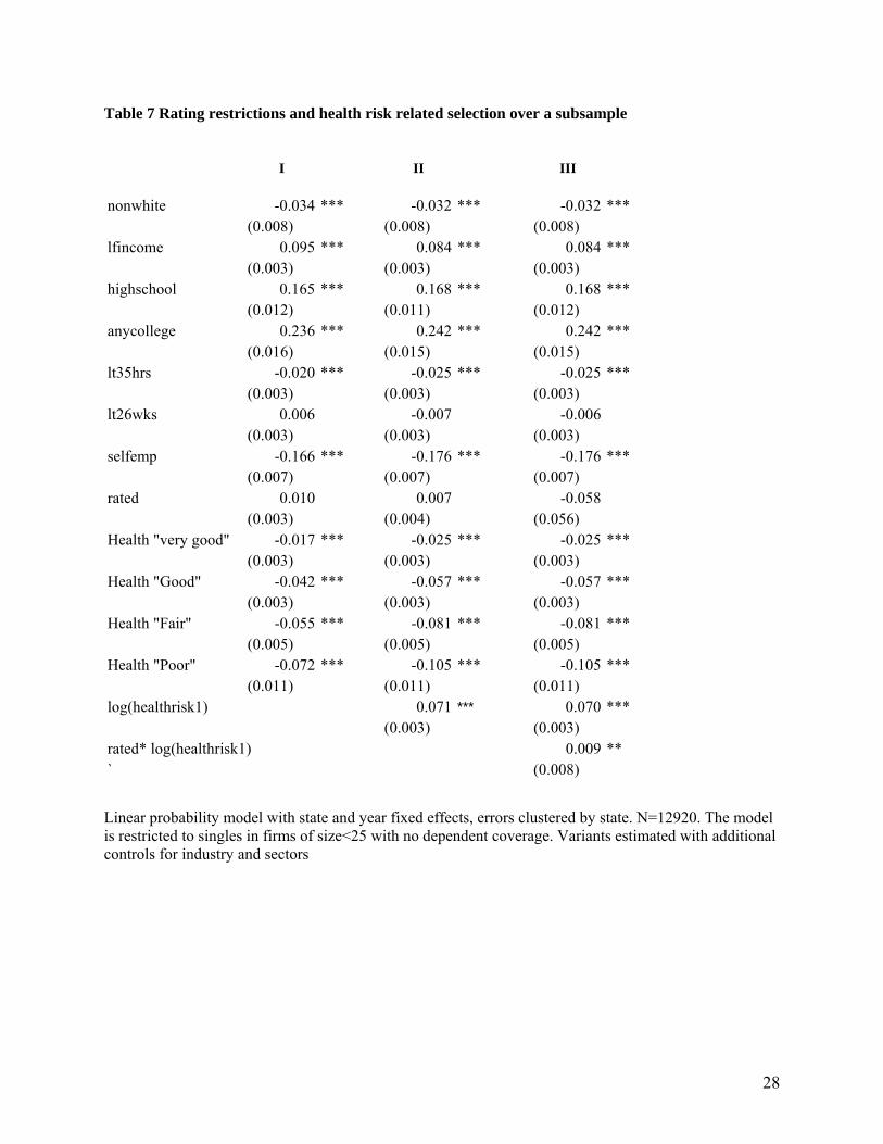
Table 7 presents results on selection using the measure Healthrisk1. Column III suggests that

residing in a community rated state increases the probability of an individual with higher expected health

expenses to purchase insurance. This might appear at odds with the result that poorer self-reported health

status is associated with lower purchase of insurance, but is consistent with the variables that drive

variation in Healthrisk1 (age and gender).

To assess if price variation has a differential role in affecting risk composition in community

rated states, I modify (4) above to estimate a model

The coefficient of interest is now 6γ . If subsidies have a role in preventing lower risks from

exiting the market for insurance in a community rated state, we would expect 6γ to be negative.

Table 8 presents results from Table 7 when the role of subsidies is accounted for. Columns I and II

suggest that tax prices matter—facing a one percent decline in tax price is associated with an increase

of .07 in the probability of purchasing insurance. The interaction of log(healthrisk1) and log(taxprice) in

Column III indicates that facing higher taxes—or lower subsidies—reduces the participation of those with

larger expected health expenses. Finally, column IV suggests that higher tax prices lower the

participation of more expensive individuals in community rated states. Put another way, receiving a larger

subsidy is differentially beneficial to individuals with lower health expenses in community rated states.

εγγγβ

effects year effects state 3 healthrisk* CR * CR CR X ed)Prob(insur

++++++= 21

εγγγ

γγγβ

effects year effects state6 healthrisk* CR*ce)log(taxpri 5CRtaxprice 4taxprice

3 healthrisk* CR CR CR X ed)Prob(insur

++++++

+++=*)log()log(

21

15

VI. Conclusion

The models estimated in the present study give credence to the concern that community rating restrictions

operate to change the profile of participants in the market for insurance, while subsidies—at least in the

context of subsidies implicitly induced by the tax system. From a policy standpoint, a subsidy offered

explicity, or one targeted better than the tax subsidy is likely to have an impact of a different magnitude.

The paper throws some light on considerations for how states might go about improving coverage. While

the take-up decision tends to be relatively insensitive to tax subsidies, premium subsidies likely impact

the risk profile of the pool of participants. The question this leads to, and one that cannot be answered

with the present data, is which particular ways individuals respond on the dimension of generosity of plan

choice, and whether subsidies can be more targeted to preserve the incentive for healther individuals to

participate, while also improving risk adjustment in insurance pools

16

REFERENCES Andreoni, J., 2006. “Philanthropy” in S-C. Kolm and J. Mercier Ythier, eds., Handbook of Giving, Reciprocity and Altruism, Amsterdam: North Holland, 2006, page 1201-1269 Auerbach, D and Ohri, S, 2006. “Price and the Demand for Non-Group Health Insurance,” Inquiry, 43(2), 122-134. Bertrand,M., Esther Duflo, D and Mullainathan,S., 2004. "How Much Should We Trust Differences-in-Differences Estimates?"; Quarterly Journal of Economics, 2004, 119(1), pp. 249-75. Buchmueller, T.C., and DiNardo, J., 2002. “Did Community Rating Induce an Adverse Selection Death Spiral? Evidence from New York, Pennsylvania and Connecticut,” American Economic Review, 92(1): 280-94. Cutler, D.M., and R.J. Zeckhauser, 1998. "Adverse selection in health insurance", in: A. Garber, ed., Frontiers in Health Policy Research, Vol. 1 (MIT Press, Cambridge, MA) 1-31. Heistaro, S, Jousilahti, P, Lahelma, E, Vartiainen, E, Puska, P, 2001. “Self rated health and mortality: a long term prospective study in eastern Finland.”J Epidemiol Community Health 55: 227-232 Herring, B., and M. Pauly, 2001. “Premium Variation in the Individual Insurance Market,” International Journal of Health Care Finance and Economics 1.1, 43-58. Lo Sasso, A.T., and Lurie I.Z., “Community Rating and the Market for Private Non-Group Health Insurance,” April 2007

Pauly, M. V., and L. M. Nichols, 2002. "The Non-Group Insurance Market: Short on Facts, Long on Opinions and Policy Disputes"

Pauly, M.V., A. Percy, and B. Herring, 1999. "Individual Versus Job-Based Health Insurance: Weighing the Pros and Cons." Health Affairs 18 (96): 28-44

Rothschild, M. and J.E. Stiglitz, 1976. “Equilibrium in Competitive Insurance Markets: An Essay on the Economics of Imperfect Information.” Quarterly Journal of Economics; 90(4):629-649. Royalty, A. B., 2000.Tax Preferences for Fringe Benefits and Workers' Eligibility for Employer Health Insurance, Journal of Public Economics, 75(2): 209-227. Selden, T., 1999. Premium Subsidies for Health Insurance: Excessive Coverage vs. Adverse Selection, Journal of Health Economics, 18: 709-725. Simon, K. 2005. "Adverse Selection in Health Insurance Markets: Evidence from State Small-Group Health Insurance Reforms".Journal of Public Economics, 89, pp.1865-1877. Turnbull, N.C. and Nancy M. Kane, N.M., 2005. Insuring the Healthy or Insuring the Sick? The Dilemma of Regulating the Individual Health Insurance Market Findings from a Study of Seven States. The Commonwealth Fund. Wachenheim L and Leida H, 2007 "The Impact of Guaranteed Issue and Community Rating Reforms on Individual Insurance Markets," report prepared by Milliman, Inc. on behalf of America’s Health Insurance Plans, August 2007

17

Wealth, health loss

W

Wealth, no health loss

FL

FH

P1

SL

O

O´

W´

ŪL

ŪH

P3

P2

Tables and Figures

Figure 1: Rothschild-Stiglitz separation and community-rating induced pooling.

Figure 2: Coverage without and with a subsidy

Q1 Q3 Qeff Quantity (take-up ) With a subsidy With adverse selection

A D E B F C

Average cost Marginal Cost Demand curve with subsidy

Price

Demand curve

18

Table 1: Community rating restrictions in state non-group markets

State Type of restriction Date of introduction

New YorkPure community rating, only differing by region April 1993

VermontModified CR for indemnity, pure CR for HMOs/ Blue Cross plans July 1993

New Jersey Pure CR August 1993

Maine

Modified CR, not allowed to vary by health, rating band of 1.5:1 for age December 1993

New Hampshire

Modified CR, rating band 3:1 for age, 1.2:1 for health. Repealed 2003 January 1995

WashingtonModified CR, band of 2:1 for age and 1.2:1 for health in 2002 January 1996

Kentucky

Modified, initially 3:! Band for age/geography/family composition but not health. Later allowed to vary 5:1. Repealed 1998 July 1996

Massachusetts

Modified CR, not allowed to vary by health, rating band of 1.33:1 for age August 1996

Sources: Auerbach and Ohri (2006), LoSasso and Lurie (2007), Wachenheimand Leida (2007)

19

Figure 3: Schedule of self-employed health Figure 4: Variation in tax price

deduction allowable as adjustment to income

Figure 5: Variation in tax price and variation in fraction insured over time in CR states

Panel A

Panel B

Tax subsidy (% premium)

0

20

40

60

80

100

120

1986

1988

1990

1992

1994

1996

1998

2000

2002

2004

2006

Variation in mean taxprice within CR states, 1994 vs 2001

mean tp nonselfmp 94

mean tp selfemp 94

mean tp nonselfmp 01

mean tp selfemp 01

0.5

0.6

0.7

0.8

0.9

1

1 2 3 4 5 6 7 8 9 10

Income decile

Mea

n ta

x pr

ice

Mean tax price by income decile, 1994

0.600

0.700

0.800

0.900

1.000

1 2 3 4 5 6 7 8 9 10

Income decile

Mea

n ta

x pr

ice

uninsured

insured

Variation in fraction insured within CR states, 1994 vs 2001

0.200

0.300

0.400

0.500

0.600

0.700

0.800

0.900

1.000

1 2 3 4 5 6 7 8 9 10

Income decile

Mea

n ta

x pr

ice

mean insurednonselfmp 94mean insured selfemp94

mean insurednonselfmp 01

mean insured selfemp01

20

Table 2: Summary statistics

1994 2001Unreg CR Unreg CR

Age 37.60 37.61 38.33 38.61(0.066) (0.161) (0.062) (0.13)

Female 0.34 0.39 0.43 0.44(0.003) (0.006) (0.002) (0.005)

Married 0.44 0.41 0.42 0.40(0.003) (0.006) (0.002) (0.005)

Nonwhite 0.17 0.19 0.19 0.18(0.002) (0.005) (0.002) (0.004)

Family income 35103.03 38120.68 49367.19 54032.51(172.318) (471.679) (271.413) (643.825)

Insured 0.77 0.76 0.77 0.78(0.002) (0.006) (0.002) (0.004)

Self employed 0.10 0.07 0.08 0.07(0.003) (0.006) (0.002) (0.005)

Nongroup insured 0.24 0.24 0.24 0.20

(0.004) (0.01) (0.004) (0.008)Healthy 0.89 0.93 0.90 0.90

(0.003) (0.006) (0.003) (0.006)Health2 1429.43 1726.54 2060.24 2488.04

(7.951) (22.55) (10.575) (28.683)Taxprice 0.79 0.78 0.79 0.79

(0.002) (0.004) (0.001) (0.003)

CR stands for Community Rated (the 8 states of NY, VT, NJ, ME, NH, WA, KY, MA). Sample means and standard errors are computed using CPS person weights. Healthy stands for individuals with self-reported health good/verygood or excellent. Health2 is a measure of individual health status computed as expected health expenses accounting for gender/age/state of residence/year, measured in year 2004 dollars.

21

Figure 6: Self reported health status by community rating status 1994

0.5

0.5

0 2 4 6 0 2 4 6

0, 0 0, 1

1, 0 1, 1

Frac

tion

Health conditionGraphs by rated and indins

2001

0.2

.40

.2.4

0 2 4 6 0 2 4 6

0, 0 0, 1

1, 0 1, 1

Frac

tion

Health conditionGraphs by rated and indins

unrated, uninsured unrated, non-group

rated, non-grouprated, uninsured

unrated, uninsured unrated, non-group

rated, non-grouprated, uninsured

22

0.0

2.0

4.0

6Fr

eque

ncy

1994

20 30 40 50 60Age

FractionFraction

Figure 7: Age distribution of nongroup market participants

Community rated states Unregulated states 0

.02

.04

.06

Freq

uenc

y 19

94

20 30 40 50 60Age

FractionFraction

1994 2001

1994 2001

23

Figure 8: Distribution of health status measure

1994 0

.05

.10

.05

.1

6 7 8 9 6 7 8 9

0, 0 0, 1

1, 0 1, 1

Fractionkdensity lprem1

Frac

tion

lprem1

Graphs by rated and indins

2001

0.0

2.0

4.0

6.0

80

.02

.04

.06

.08

6 7 8 9 6 7 8 9

0, 0 0, 1

1, 0 1, 1

Fractionkdensity lprem1

Frac

tion

lprem1

Graphs by rated and indins

Health2 is a measure of individual health status computed as expected health expenses accounting for gender/age/state of residence/year, measured in year 2004 dollars.

Log(health2 )

Log(health2 )

unrated, uninsured unrated, non-group

rated, non-grouprated, uninsured

unrated, uninsured unrated, non-group

rated non-grouprated, uninsured

24

Table 3: Linear probability model of private non-group market participation on covariates N=396,698. Linear probability model with state and year fixed effects, errors clustered by state.Emplsz stands for categories of firm size

I IIAge 25-29 -0.045 *** -0.045 ***

(0.004) (0.004)30-34 -0.049 *** -0.049 ***

(0.005) (0.005)35-39 -0.041 *** -0.041 ***

(0.005) (0.005)40-44 -0.036 *** -0.036 ***

(0.005) (0.005)45-49 -0.034 *** -0.034 ***

(0.005) (0.005)50-54 -0.029 *** -0.029 ***

(0.005) (0.005)55-59 -0.019 *** -0.019 ***

(0.005) (0.005)60-64 -0.010 * -0.010

(0.006) (0.006)female 0.003 ** 0.003 **

(0.001) (0.001)nonwhite -0.016 *** -0.016 ***

(0.002) (0.002)married -0.029 *** -0.029 ***

(0.002) (0.002)kidpresent 0.002 * 0.002 *

(0.001) (0.001)lfincome -0.007 *** -0.007 ***

(0.002) (0.002)highschool 0.026 *** 0.026 ***

(0.002) (0.002)anycollege 0.053 *** 0.053 ***

(0.004) (0.004)less than35hrs 0.049 *** 0.049 ***

(0.003) (0.003)less than 26 wk 0.019 *** 0.019 ***

(0.003) (0.003)agmincon -0.048 ** -0.048 **

(0.013) (0.013)manuf -0.046 ** -0.046 **

(0.013) (0.013)services -0.037 ** -0.037 **

(0.013) (0.013)_Iemplsz_1 0.087 *** 0.087 ***

(0.015) (0.015)_Iemplsz_2 0.042 ** 0.042 **

(0.015) (0.015)_Iemplsz_3 0.023 0.023

(0.014) (0.014)_Iemplsz_4 0.012 0.012

(0.015) (0.015)_Iemplsz_5 0.008 0.008

(0.015) (0.015)_Iemplsz_6 0.006 0.006

(0.015) (0.015)selfemp 0.135 *** 0.135 ***

(0.007) (0.007)rated 0.000

(0.003)Years since CR -0.002 **

25

Table 4: Coefficients on rated (or years since CR) from linear probability models similar to Table 3

Non-group insurance Uninsured

Coefficient on Rated Years since CR Rated Years since CR

Full sample N=396,6980.000 -0.002 -0.012 * -0.001

(0.001) (0.001) (0.003) (0.001)

Healthy A: Individuals in "excellent" health, N=137,446-0.009 -0.004 * 0.008 0.001

(0.006) (0.001) (0.007) (0.001)

Healthy B: Single men, age 19-35 in "excellent" health, N=40055-0.017 -0.004 * -0.012 * 0.001

(0.010) (0.001) (0.001) (0.001)

Unhealthy AHealth=fair or poor, N=279730.031 * 0.003 * -0.073 * -0.004

(0.008) (0.001) (0.019) (0.001)Unhealthy Age 40+, Health fair or poor, N=19225

0.042 * 0.006 * -0.114 * -0.004(0.006 0.002 0.004 -0.005

Linear probability model with state and year fixed effects, errors clustered by state, model as in Table 3,

estimated over the subsamples indicated.

26

Table 5: Results on selection in community rated states. Dependent variable: privately insured

I IIage 0.002 *** 0.002 ***

(0) (0)nonwhite -0.056 *** -0.056 ***

(0.008) (0.008)kidpresent 0.014 *** 0.016 ***

(0.002) (0.003)lfincome 0.084 *** 0.073 ***

(0.002) (0.002)highschool 0.155 *** 0.152 ***

(0.01) (0.009)anycollege 0.226 *** 0.224 ***

(0.014) (0.014)lt35hrs -0.037 *** -0.027 ***

(0.003) (0.003)selfemp -0.059 *** -0.018

(0.006) (0.008)healthy2 0.025 *** 0.024 ***

(0.003) (0.003)CR 0.033 *** -0.024 **

(0.005) (0.007)Affected -0.183 *** -0.184 ***

(0.012) (0.012)Affected*Healthy2 0.063 *** 0.065 ***

(0.006) (0.006)CR*Healthy2 0.013 * 0.013 *

(0.005) (0.005)CR*Affected -0.014 -0.013

(0.016) (0.016)CR*Affected*Healthy2 -0.012 -0.013

(0.008) (0.008)Log(tax price) -0.129 ***

(0.013)

N=348122. Linear probability model of being insured. Standard errors clustered by state. Affected=1 if in a firm of size 25 or below, and/or self-employed. CR=indicator for being in a state with nongroup or/and smallgroup community rating restrictions. Healthy2=indicator for being in very good or excellent health.

27

Table 5: Selection and subsidies, effect of tax price on interactions in model in Table 4 I II III

age 0.002 *** 0.002 *** 0.002 ***(0) (0) (0)

nonwhite -0.056 *** -0.056 *** -0.056 ***(0.008) (0.008) (0.008)

kidpresent 0.017 *** 0.017 *** 0.017 ***(0.002) (0.002) (0.002)

lfincome 0.074 *** 0.074 *** 0.074 ***(0.002) (0.002) (0.002)

highschool 0.151 *** 0.151 *** 0.151 ***(0.01) (0.01) (0.01)

anycollege 0.222 *** 0.222 *** 0.222 ***(0.014) (0.014) (0.014)

lt35hrs -0.024 *** -0.025 *** -0.024 ***(0.003) (0.003) (0.003)

selfemp -0.028 ** -0.028 ** -0.027 **(0.009) (0.009) (0.009)

healthy2 0.099 *** 0.100 *** 0.110 ***(0.008) (0.008) (0.008)

CR -0.024 ** -0.035 * -0.035 *(0.007) (0.012) (0.012)

Affected -0.167 *** -0.168 *** -0.169 ***(0.014) (0.013) (0.015)

Affected*Healthy2 0.054 *** 0.054 *** 0.052 ***(0.006) (0.006) (0.006)

CR*Healthy2 0.012 * 0.011 0.011(0.004) (0.004) (0.004)

CR*Affected -0.012 -0.011 0.015(0.016) (0.015) (0.018)

CR*Affected*Healthy2 -0.014 -0.014 -0.051 **(0.008) (0.008) (0.014)

Log(tax price) -0.256 *** -0.239 *** -0.255 ***(0.014) (0.028) (0.029)

Affected*Log(tax price) 0.027 0.027 0.022(0.013) (0.013) (0.023)

Healthy2*Log*(tax price) 0.188 0.188 *** 0.214 ***(0.016) (0.016) (0.017)

CR* log(tax price) -0.024 -0.026(0.032) (0.033)

CR* Affected* log(tax price) 0.083 **(0.027)

CR* Affected*Healthy2* log(tax price) -0.113 ***(0.028)

N=348122. Linear probability model of being insured. Standard errors clustered by state. Affected=1 if in a firm of size 25 or below, and/or self-employed. CR=indicator for being in a state with nongroup or/and smallgroup community rating restrictions. Healthy2=indicator for being in very good or excellent health.

28

Table 7 Rating restrictions and health risk related selection over a subsample

I II III

nonwhite -0.034 *** -0.032 *** -0.032 ***(0.008) (0.008) (0.008)

lfincome 0.095 *** 0.084 *** 0.084 ***(0.003) (0.003) (0.003)

highschool 0.165 *** 0.168 *** 0.168 ***(0.012) (0.011) (0.012)

anycollege 0.236 *** 0.242 *** 0.242 ***(0.016) (0.015) (0.015)

lt35hrs -0.020 *** -0.025 *** -0.025 ***(0.003) (0.003) (0.003)

lt26wks 0.006 -0.007 -0.006(0.003) (0.003) (0.003)

selfemp -0.166 *** -0.176 *** -0.176 ***(0.007) (0.007) (0.007)

rated 0.010 0.007 -0.058(0.003) (0.004) (0.056)

Health "very good" -0.017 *** -0.025 *** -0.025 ***(0.003) (0.003) (0.003)

Health "Good" -0.042 *** -0.057 *** -0.057 ***(0.003) (0.003) (0.003)

Health "Fair" -0.055 *** -0.081 *** -0.081 ***(0.005) (0.005) (0.005)

Health "Poor" -0.072 *** -0.105 *** -0.105 ***(0.011) (0.011) (0.011)

log(healthrisk1) 0.071 *** 0.070 ***(0.003) (0.003)

rated* log(healthrisk1) 0.009 **` (0.008)

Linear probability model with state and year fixed effects, errors clustered by state. N=12920. The model is restricted to singles in firms of size<25 with no dependent coverage. Variants estimated with additional controls for industry and sectors

29

Table 8: Differential role of tax prices over healthrisk for the model in Table 7 I II III IV

` -0.032 *** -0.032 *** -0.033 *** -0.033 ***(0.008) (0.008) (0.008) (0.008)

lfincome 0.079 *** 0.079 *** 0.079 *** 0.079 ***(0.002) (0.002) (0.002) (0.002)

highschool 0.167 *** 0.167 *** 0.167 *** 0.167 ***(0.011) (0.011) (0.011) (0.011)

anycollege 0.242 *** 0.242 *** 0.240 *** 0.240 ***(0.015) (0.015) (0.015) (0.015)

lt35hrs -0.022 *** -0.022 *** -0.022 *** -0.022 ***(0.003) (0.003) (0.003) (0.003)

lt26wks -0.001 -0.001 -0.001 -0.001(0.004) (0.004) (0.004) (0.004)

selfemp -0.152 *** -0.152 *** -0.150 *** -0.150 ***(0.01) (0.01) (0.01) (0.01)

rated -0.055 -0.053 -0.045 0.120(0.056) (0.058) (0.057) (0.1)

Health "very good" -0.025 *** -0.025 *** -0.025 *** -0.025 ***(0.003) (0.003) (0.003) (0.003)

Health "Good" -0.057 *** -0.057 *** -0.057 *** -0.057 ***(0.003) (0.003) (0.003) (0.003)

Health "Fair" -0.081 *** -0.081 *** -0.080 *** -0.080 ***(0.005) (0.005) (0.005) (0.005)

Health "Poor" -0.103 *** -0.103 *** -0.100 *** -0.100 ***(0.011) (0.011) (0.011) (0.011)

log(healthrisk1) 0.070 *** 0.070 *** 0.045 *** 0.048 ***(0.003) (0.003) (0.008) (0.008)

rated* log(healthrisk1) 0.008 0.009 0.008 -0.013` (0.007) (0.007) (0.007) (0.012)log (tax price) -0.072 ** -0.075 ** 0.449 ** 0.379 *

(0.02) (0.023) (0.13) (0.134)rated * log(tax price) 0.018 0.031 0.494 *

(0.029) (0.029) (0.172)log(healthrisk)*log(taxprice) -0.070 *** -0.061 ***

(0.015) (0.016)rated* log(healthrisk)*log(taxprice) -0.061 **

(0.02)

Linear probability model with state and year fixed effects, errors clustered by state. N=12920. The model

is restricted to singles in firms of size<25 with no dependent coverage. Variants estimated with additional

controls for industry and sectors