Adverse Selection in Secondary Insurance Markets: … · Adverse Selection in Secondary Insurance Markets: Evidence from the Life ... although in a secondary market ... for the settled

Adverse Selection in Secondary Insurance Markets:Evidence from the Life Settlement Market ∗

Daniel Bauer†

Department of Risk Management and Insurance, Georgia State University

35 Broad Street, 11th Floor; Atlanta, GA 30303; USA

Jochen RussInstitut fur Finanz- und Aktuarwissenschaften and Ulm University

Lise-Meitner-Straße 14; 89081 Ulm; Germany

Nan ZhuDepartment of Mathematics, Illinois State University

100 N University Street; Normal, IL 61790; USA

August 2014

Abstract

We use data from a large US life expectancy provider to test for asymmetric information in

the secondary life insurance—or life settlement—market. We compare the average difference

between realized lifetimes and estimated life expectancies for a sub-sample of settled policies

relative to the entire sample. We find a significant positive difference indicating private infor-

mation on mortality prospects. Using non-parametric estimates for the excess mortality and

survival regressions, we show that the informational advantage is temporary and wears off over

five to six years. We argue this is in line with adverse selection on an individual’s condition,

which has important economic consequences for the life settlement market and beyond.

JEL classification: D12; G22; J10

Keywords: Life Settlements; Life Expectancy; Asymmetric Information; Adverse Selection

∗We are grateful for support from Fasano Associates, especially to Mike Fasano. Moreover, we thank seminarparticipants at Georgia State University and the 2014 NBER insurance workshop, in particular, Stephen Shore, LiranEinav, Lauren Cohen, Ken Froot, Greg Niehaus, and Richard Phillips for valuable comments. Bauer and Zhu alsogratefully acknowledge financial support from the Society of Actuaries under a CAE Research Grant.†Corresponding author. Phone: +1-(404)-413-7490. Fax: +1-(404)-413-7499. Email addresses: [email protected]

(Bauer); [email protected] (Russ); [email protected] (Zhu).

1

ADVERSE SELECTION IN SECONDARY INSURANCE MARKETS 2

1 Introduction

Although seminal theoretical contributions have emphasized the significance of asymmetric in-formation for a market’s functioning since the 1960s (Arrow, 1963; Akerlof, 1970; Rothschildand Stiglitz, 1976), the corresponding empirical literature has flourished only relatively recently.1

In this context, several contributions highlight the merits of insurance data for testing theoreticalpredictions (Cohen and Siegelman, 2010; Chiappori and Salanie, 2013), although heterogeneityalong multiple dimensions may impede establishing or characterizing informational asymmetries(Finkelstein and McGarry, 2006; Cohen and Einav, 2007; Cutler et al., 2008; Fang et al., 2008).One market segment that offers the benefits of insurance data but is not subject to confoundingfactors—or at least, not to the same confounding factors—is the secondary insurance market, yetthis aspect to our knowledge has not been explored thus far.

In this paper, we provide evidence for asymmetric information in the secondary life insur-ance market, the market for so-called life settlements. Within such a transaction, a policyholdersells—or settles—her life-contingent insurance benefits for a lump sum payment, where the offeredprice depends on an individualized evaluation of her survival probabilities by a third party life ex-

pectancy provider (LE provider). In particular, using the full dataset of a large US LE provider,we show that individuals have significant private information regarding their mortality prospectsthat is particularly pronounced in the early period after settling but is “decreasing” in the sense thatthe informational advantage wears off over about five to six years. We argue that such a patternis in line with “hidden information” with respect to the current health state but does not coherewith “hidden actions” that affect future survival probabilities. As such, we can characterize theinformational friction as adverse selection rather than moral hazard.2

Of course, our results are of immediate interest and have implications for the life settlementmarket, for instance in view of pricing the transactions (Zhu and Bauer, 2013). However, whilenaturally our quantitative results are specific to our setting, we believe our qualitative insights lendthemselves to draw broader conclusions. On the one hand, with regards to primary life insurancemarkets, our results reinforce the insight that individuals have private information on their life-time distribution and make use of it, despite the mixed evidence from corresponding studies. Inparticular, our characterization supports the proposition from various authors that informationalasymmetries in these markets originate from adverse selection rather than moral hazard, whichpreviously were based on “intuitive insight rather than on rigorous evidence” (He, 2009). On the

1See, e.g., Puelz and Snow (1994), Cawley and Philipson (1999), Chiappori and Salanie (2000), Cardon and Hendel(2001), Finkelstein and Poterba (2004), Cohen (2005), Finkelstein and McGarry (2006), or Cohen and Einav (2007).

2Our findings are in line with a recent industry study by Granieri and Heck (2013) that postdates the first draftof our paper. More precisely, based on simple comparisons of survival curves for different populations, the authorsconclude that within the life settlement market, “insureds use the proprietary knowledge of their own health to selectagainst the investor.”


other hand, our results suggest that individuals more broadly are competent in predicting their rel-ative survival prospects, possibly in contrast to their ability in predicting absolute life expectanciesthat may be subject to framing and other behavioral biases (Payne et al., 2013). We believe thatthe former task may be more material for retirement planning given that individuals may be pro-vided with background information on “typical” life expectancies or suitable “default” choices foraverage individuals.

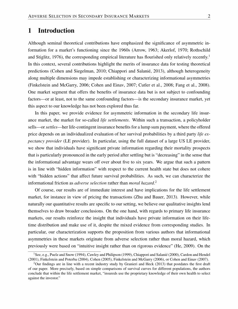
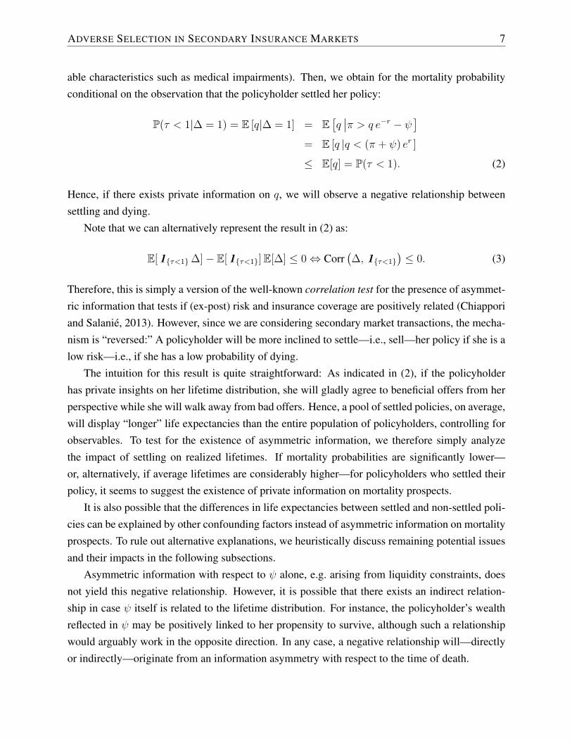
Our empirical strategy relies on comparisons of mortality forecasts for the entire sample, con-sisting of policyholders that settled their policies and those that did not, with a subsample in whicheveryone is known to have settled their policy. Figure 1, the construction of which we describein much more detail in Section 3, illustrates our basic result. Here, we plot multiplicative “excessmortality” for individuals that we know have settled their policy over time since the person’s lifeexpectancy was evaluated (blue solid curve). Naturally, if this curve had the shape of a horizontalline at one (black dotted line) or if the horizontal line at one would fall within the 95% confidenceintervals (red dashed curves), we would conclude that there is no (significant) effect of settling onan individual’s mortality pattern. The observation that this curve is overall less than one, partic-ularly over the early years after underwriting, implies that there is a negative association betweensettling and the instantaneous mortality probability. Thus, policyholders who settled their policies,on average, live longer. This result corresponds to the so-called positive correlation test for asym-metric information that tests the basic prediction of a positive relationship between (ex-post) riskand purchasing insurance coverage (Chiappori and Salanie, 2000, 2013), although in a secondarymarket setting, the mechanism is “reversed.” Here, a policyholder will be more inclined to sell

her policy if she is a “low risk”—i.e., if she has a low probability of dying. Hence, the observednegative relationship documents the existence of asymmetric information in the life settlementmarket.

An alternative (and simpler) approach to establishing this negative relationship is comparing theaverage difference in realized partial life spans (to date) and estimated temporary life expectancies(DTLE) for the entire sample and the subsample of settled policies. We find that for the entiresample, the average DTLE is around one month. This indicates that overall the life expectancyevaluations are fairly accurate and, at least for the LE provider in view, do not exhibit a considerablepositive bias as opposed to findings by other authors that may have been based on data fromdifferent LE providers (Gatzert, 2010). In contrast, for the settled cases, the difference betweenrealized and estimated temporary life expectancies is significantly greater and amounts to aroundfour months, also demonstrating the negative relationship between mortality and settling underasymmetric information.

In addition to the existence of asymmetric information, Figure 1 illustrates the pattern over


Figure 1: Excess mortality for settled subsample

time, which in turn provides insights on the characteristics of the informational friction.3 Moreprecisely, we observe that the informational advantage is particularly pronounced in the early yearsafter underwriting but that it is decreasing in the sense that it wears off over five to six years. Sucha structure is akin to so-called select-and-ultimate life tables in actuarial or demographic studiesthat capture temporary selection effects, and thus is in line with (adverse) selection on the initialhealth condition. In contrast, if the negative relationship were driven by hidden actions (moralhazard) such as a healthier lifestyle choice or other changes in behavior after settling, we wouldexpect to see a steady or increasingly pronounced relationship over time.

To ascertain that our results are not driven by idiosyncrasies of our sample of settled policies,we run detailed semi-parametric survival regressions controlling for observables. In particular, weinclude the estimated force of mortality from the LE provider as well as all observable charac-teristics such as the time of underwriting, the primary impairment, etc. as explanatory variables.4

Several—though not all—of the (known) primary impairment dummies fail to be significant, indi-cating that the LE provider’s estimates correctly account for these. In contrast, having settled thepolicy (unknown to the LE provider at the time of underwriting) has a significant negative effect onthe force of mortality, particularly when also considering a linear trend. The slope of the trend is

3The idea to consider dynamic relationships to characterize asymmetric information already occurs in Abbring etal. (2003) in the context of experience ratings in automobile insurance.

4Chiappori and Salanie (2000) and Dionne et al. (2005) emphasize the importance of accounting for all pricing-relevant observed covariates.


significant and positive, implying that the effect becomes weaker over time. Hence, the results ofthe survival regressions reinforce the insights from the aggregate non-parametric estimate shownin Figure 1: We find evidence for asymmetric information, though the informational advantagewears off over time—in line with adverse selection on the initial condition.

To appraise the quantitative impact, we then rely on the regression results to calculate theimplications of the settlement decision on an “average” individual’s life expectancy. We find thatthe effect is economically significant and, for a 75-year old male, amounts to around two yearswhen considering the basic (constant) effect and around eight months when accounting for thetemporary pattern, depending on the total proportion of settled policies in our dataset.

However, assessing the economic impact of adverse selection on the life settlement marketwill not be possible without putting in place more structure on the policyholder’s decision process(Einav et al., 2007, 2010a). In particular, for answering policy-relevant questions regarding effi-ciency and welfare implications of this market, it is necessary to consider and estimate equilibriummodels that also account for barriers to participate in this market (Einav et al., 2010b) and reper-cussions on primary insurance (Daily et al., 2008; Fang and Kung, 2010; Zhu and Bauer, 2011).While such questions are beyond the scope of this paper, we believe they are intriguing problemsfor future research.

Relationship to the Literature

Of course, there is an array of papers analyzing the existence of information asymmetries in in-surance markets (see Footnote 1 for a selection). For life contingencies, Finkelstein and Poterba(2002, 2004) establish that there exists asymmetric information in the market for life annuities,whereas the evidence for life insurance is mixed (Cawley and Philipson, 1999; He, 2009; Mc-Carthy and Mitchell, 2010; Wu and Gan, 2013). Cohen and Siegelman (2010) posit that theseseemingly contrasting findings may be explained by a positive relationship between income andinsurance coverage: A higher wealth or income may be negatively associated with mortality riskbut positively associated with insurance coverage. Thus, it is not clear whether the evidence isdue to confounding factors that are not priced (wealth, risk aversion) or a “true” informationaladvantage. In contrast, the pricing of life settlements is highly individualized, and wealth effectsshould, if they are present at all, imply that sicker people are more likely to settle (since sick peo-ple may be more wealth-constraint). Hence, our findings present crisper evidence that individualspossess—and make use of—superior information regarding their mortality prospects. Moreover,we complement the above studies in that we are able to provide insights on the characteristics ofthe informational friction that are in line with adverse selection.

More broadly, our results provide new evidence on individuals’ ability to forecast their own


mortality prospects. Recent contributions to the behavioral literature provide negative results in thisdirection, with forecasts differing according to the framing of corresponding questions and beingsubject to various biases (Elder, 2013; Payne et al., 2013; and references therein). However, thesestudies consider forecasts of absolute life expectancies. Our results indicate that individuals appearto fare better when evaluating their relative mortality prospects, which may be the more materialtask for retirement planning given that individuals can be provided with background informationon population mortality averages or “default” choices that are suitable for average individuals.

2 A Simple Model

This section presents a simple one-period model to provide the intuition for our empirical analysisof the existence of asymmetric information in the life settlement market. We assume that at timezero, the policyholder is endowed with a one-period term-life insurance policy that pays $1 at timeone in case of death before time one and nothing in case of survival thereafter. The probability fordying before time one is P(τ < 1) = q, where τ is the time of death.

Suppose the policyholder is offered a life settlement at price π. For simplicity, we assume sheassesses her settlement decision ∆ = 1{policyholder settles} by comparing the settlement price to thepresent value of her contract:

∆ = 1⇔ π > q e−r − ψ, (1)

where r is the risk-free interest rate and ψ characterizes the policyholder’s proclivity for settling.The latter may originate from risk-averse policyholder preferences with a bequest motive as in Zhuand Bauer (2013) or from liquidity constraints. Here, we simply use ψ to capture deviations froma value-maximizing behavior, under which the market may collapse due to a “lemons problem” asin Akerlof (1970).

2.1 Basic Case

We first assume that the policyholder has private information on the mortality probability q. There-fore, from the policyholder’s perspective, the question of whether or not to settle the policy basedon Equation (1) is deterministic. However, this may not be the case from the perspective of thelife settlement company offering to purchase the policy since it may have imperfect informationwith respect to q and/or ψ.5 In particular, assume that the life settlement company solely observesthe expected value, E[q], across the entire population (potentially conditional on various observ-

5Of course, such an information asymmetry may affect the pricing of the transaction, i.e. the choice of π. We referto Zhu and Bauer (2013) for a corresponding analysis. Here, we focus on the implications when the settlement priceis given.


able characteristics such as medical impairments). Then, we obtain for the mortality probabilityconditional on the observation that the policyholder settled her policy:

P(τ < 1|∆ = 1) = E [q|∆ = 1] = E[q∣∣π > q e−r − ψ

]= E [q |q < (π + ψ) er ]

≤ E[q] = P(τ < 1). (2)

Hence, if there exists private information on q, we will observe a negative relationship betweensettling and dying.

Note that we can alternatively represent the result in (2) as:

E[ 1{τ<1}∆]− E[ 1{τ<1}]E[∆] ≤ 0⇔ Corr(∆, 1{τ<1}

)≤ 0. (3)

Therefore, this is simply a version of the well-known correlation test for the presence of asymmet-ric information that tests if (ex-post) risk and insurance coverage are positively related (Chiapporiand Salanie, 2013). However, since we are considering secondary market transactions, the mecha-nism is “reversed:” A policyholder will be more inclined to settle—i.e., sell—her policy if she is alow risk—i.e., if she has a low probability of dying.

The intuition for this result is quite straightforward: As indicated in (2), if the policyholderhas private insights on her lifetime distribution, she will gladly agree to beneficial offers from herperspective while she will walk away from bad offers. Hence, a pool of settled policies, on average,will display “longer” life expectancies than the entire population of policyholders, controlling forobservables. To test for the existence of asymmetric information, we therefore simply analyzethe impact of settling on realized lifetimes. If mortality probabilities are significantly lower—or, alternatively, if average lifetimes are considerably higher—for policyholders who settled theirpolicy, it seems to suggest the existence of private information on mortality prospects.

It is also possible that the differences in life expectancies between settled and non-settled poli-cies can be explained by other confounding factors instead of asymmetric information on mortalityprospects. To rule out alternative explanations, we heuristically discuss remaining potential issuesand their impacts in the following subsections.

Asymmetric information with respect to ψ alone, e.g. arising from liquidity constraints, doesnot yield this negative relationship. However, it is possible that there exists an indirect relation-ship in case ψ itself is related to the lifetime distribution. For instance, the policyholder’s wealthreflected in ψ may be positively linked to her propensity to survive, although such a relationshipwould arguably work in the opposite direction. In any case, a negative relationship will—directlyor indirectly—originate from an information asymmetry with respect to the time of death.


Average (Std Dev) Count

Life Expectancy Estimate Male11.86 33,299(4.27) (63.30%)

Underwriting Age Observed Deaths75.20 7,552(7.25) (14.26%)

Table 1: Summary statistics for the entire 52,603 cases; earliest observation date.

Average (Std Dev) Count

Life Expectancy Estimate Male10.01 597(3.21) (60.12%)

Underwriting Age Observed Deaths73.53 114

(19.51) (12.22%)

Table 2: Summary statistics for the closed 933 cases; earliest observation date.

3 Data and Basic Econometrical Approach

3.1 Data

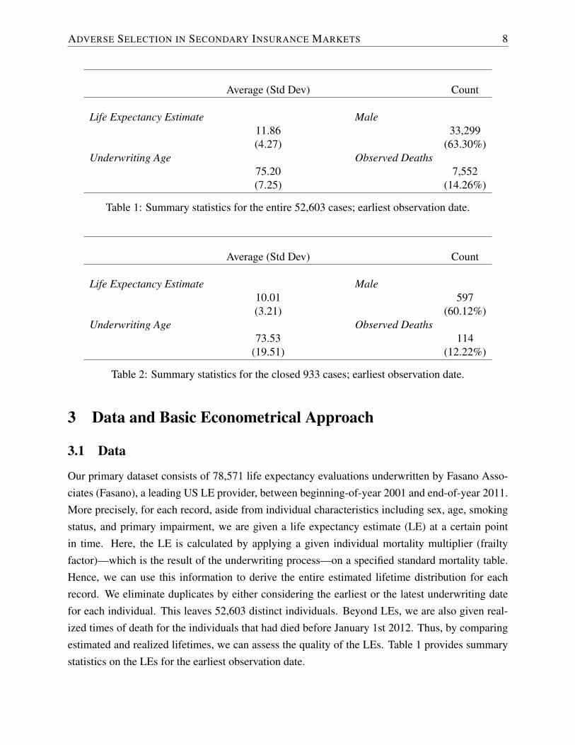
Our primary dataset consists of 78,571 life expectancy evaluations underwritten by Fasano Asso-ciates (Fasano), a leading US LE provider, between beginning-of-year 2001 and end-of-year 2011.More precisely, for each record, aside from individual characteristics including sex, age, smokingstatus, and primary impairment, we are given a life expectancy estimate (LE) at a certain pointin time. Here, the LE is calculated by applying a given individual mortality multiplier (frailtyfactor)—which is the result of the underwriting process—on a specified standard mortality table.Hence, we can use this information to derive the entire estimated lifetime distribution for eachrecord. We eliminate duplicates by either considering the earliest or the latest underwriting datefor each individual. This leaves 52,603 distinct individuals. Beyond LEs, we are also given real-ized times of death for the individuals that had died before January 1st 2012. Thus, by comparingestimated and realized lifetimes, we can assess the quality of the LEs. Table 1 provides summarystatistics on the LEs for the earliest observation date.


The full dataset contains LEs for policyholders that decided to settle their policies (so-calledclosed cases), LEs for policyholders that walked away from a settlement offer, and LEs for indi-viduals that were underwritten for different reasons. Typically, the LE provider does not receivefeedback of whether or not a policy closed, so that this aspect is unknown for our full dataset.However, we also have access to portfolio information for three life settlement investors consistingof overall 933 policies underwritten by Fasano. Hence, for this small subsample of individuals,we have the additional information that they settled their policies. We will refer to this set as thesubsample of closed policies, whereas we will refer to the rest of the sample as the remaining

cases. Table 2 provides corresponding summary statistics for the closed subsample, also based onthe earliest observation date.

We thus can compare the quality of the LEs for the closed subsample and the entire sampleto analyze whether there exists a significant (positive) difference, as suggested by the asymmetricinformation test described in the previous section. For this purpose, we need an aggregate statisticto assess the quality of a sample of (heterogeneous) LEs. The next section introduces the average

difference in realized lifetimes and projected life expectancies (DLE) and the average difference in

realized partial lifetimes and projected temporary life expectancies (DTLE) as suitable candidates.

3.2 Assessing Life Expectancy Estimates

Assume we knew the time of death for each individual in a given sample of LEs. Then, we couldcalculate the difference between the realized lifetime and the given LE in each case. For a givenindividual, of course this would be a random variable due to the intrinsic randomness of death.However, under the hypothesis that the LEs are accurate, the average of the (mean-zero) randomvariables with bounded variance should converge to zero by the law of large numbers. We refer tothis average as the average difference in realized lifetimes and projected life expectancies (DLE).

The key issue with this approach within our setting is that our death data are right-censored.That is, we only observe times of death that occurred before January 1st 2012, whereas for otherindividuals we solely know that they are still alive at this cut-off date. However, since we aregiven the entire estimated lifetime distribution, we are able to rely on an alternative concept fromactuarial science and demographic research, namely the temporary life expectancy. More precisely,for each individual i in a sample of LEs of size N , denote by τ (i) the time of death distributed withforce of mortality {µ(i)

t }t≥0, 1 ≤ i ≤ N . Then, at the cut-off date, we observe the right-censoredversion of the time of death τ (i) = min{τ (i), ti}, where ti is the (given) difference between thecut-off date and the time of underwriting, all measured in years. Its expected value, the so-calledtemporary life expectancy, is given by the integral of the survival probabilities until time ti (Bowers


et al., 1997):

e(i)ti

= E[τ (i)]

=

∫ ti

0

exp

{−∫ t

0

µ(i)s ds

}dt, 1 ≤ i ≤ N.

Denote the estimated force of mortality for individual i supplied by the LE provider by {µ(i)t }t≥0,

and denote the corresponding estimated temporary life expectancy by:

e(i)ti

=

∫ ti

0

exp

{−∫ t

0

µ(i)s ds

}dt, 1 ≤ i ≤ N.

Then, under the hypothesis that the estimated lifetime distributions are accurate, the difference inrealized partial lifetime and estimated temporary life expectancy for individual i = 1, . . . , N :

τ (i) − e(i)ti ,

is a zero-mean random variable with bounded variance.6 Thus, the average:

DTLEN =1

N

N∑i=1

[τ (i) − e(i)ti

],

which we will refer to as the average difference in realized partial lifetimes and projected tem-

porary life expectancies (DTLE), will converge to zero by Kolmogorov’s Law of Large Numbers.Moreover, with Lyapunov’s Central Limit Theorem (Billingsley, 1995), we obtain:

DTLEN1NSTRN

=1

STRN

N∑i=1

[τ (i) − e(i)ti

]→ N(0, 1), (4)

where (STRN )2 =∑N

i=1 Var[τ (i)] ≈∑N

i=1(τ(i) − e

(i)ti

)2. In particular, we can rely on (4) to drawinference on the quality of the LEs.

Table 3 provides DTLE calculations for our entire dataset, the subsample of closed cases, andthe remaining cases. The significance stars indicate the deviation from zero under the hypothesisthat the estimated lifetime distributions are accurate. We find that the DTLEs for the entire sampleamount to less than one month or slightly less than two months, depending on the observationtime. Given that LEs are only provided up to full months and that there is some arbitrariness in therounding procedure, a difference of less than one month as within the latest underwriting date isalmost negligible for practical purposes—although it is still statistically significant due to the very

6It is important to note that this hypothesis is considerably stronger than the previous hypothesis that only the LEsare accurate. In particular, our tests rely on the entire estimated distributions whereas Fasano typically only suppliesthe expected values to their clients. Thus, our tests might be too stringent to appraise the quality of their estimates.


Estimates

(1) All Cases (2) Closed Cases (3) Remaining Cases

Earliest observationN 52603 933 51670DTLE 0.1646∗∗∗ 0.4580∗∗∗ 0.1593∗∗∗1NSTRN (0.0050) (0.0368) (0.0051)

Latest observationN 52603 933 51670DTLE 0.0634∗∗∗ 0.1466∗∗∗ 0.0619∗∗∗1NSTRN (0.0047) (0.0292) (0.0048)

Table 3: Average difference in realized partial lifetimes and projected temporary life expectancies(DTLE) in years for various subsamples.

large number of observations.7

In contrast, the DTLEs for the closed cases are almost two and five months for the latest andthe earliest observation date, respectively. In particular, the (asymptotically Normal) differencebetween the closed and the remaining sample is positive and highly significant, implying thatindividuals that settled their policy in the secondary market, on average, live relatively longer.In view of the discussion from Section 2, these findings provide evidence for the existence ofasymmetric information regarding mortality prospects in the life settlement market—which is thecentral result in this paper.

Another potential explanation for this finding is that the subsample of closed policies differs insome significant way from the full sample. Before addressing this issue in Section 4 by runningdetailed survival regressions that control for all available observables, in the remainder of thissection, we analyze in more detail the time pattern of the difference in mortalities.

3.3 Non-parametric Estimation of Excess Mortality

The results in the previous subsection indicate that, ceteris paribus, mortality is significantly lowerfor individuals that settled their policy. In what follows, we derive the “excess mortality” for poli-cyholders that settled as a function of time to gain insight on the characteristics of the informationalfriction. To illustrate what we mean by “excess mortality,” assume we are given two individuals S

7The reason that the earliest observation date produces a slightly larger difference in part is explained by scaleeffects since obviously lives are observed over a longer time period. However, we also found that the estimates appearto have become more accurate over time.


and R with forces of mortality {µSt }t≥0 and {µRt }t≥0, respectively, that differ only in the informa-tion regarding their settlement decision but are otherwise identical. More precisely, assume thatwe know S settled her policy whereas the settlement decision for R is not known. Then we candefine the multiplicative excess mortality {α(t)}t≥0 and the additive excess mortality {β(t)}t≥0 viathe following relationships:

µSt = α(t)× µRt and µSt = β(t) + µRt .

Andersen and Vaeth (1989) provide non-parametric estimators for the multiplicative and addi-tive excess mortality by relying on the most popular non-parametric survival estimators, namely theNelson-Aalen (N-A) estimator for

∫ t0α(s) ds and Kaplan-Meier (K-M) estimator for

∫ t0β(s) ds,

respectively. However, their approach relies on the assumption that the “baseline” mortality (µRtin our specification) is known, whereas we only have available estimates {µ(i)

t }t≥0 given by theLE provider, 1 ≤ i ≤ N. Therefore, for the estimation of the multiplicative excess mortality, weinstead use the following three step-procedure that relies on a repeated application of the Andersenand Vaeth (1989) estimator:

1. We start with the specification:

µ(i)t = A(t)× µ(i)

t , 1 ≤ i ≤ N, (5)

and use the Andersen and Vaeth (1989) excess mortality estimator to obtain an estimate forA, say A, based on the full dataset. Hence, A corrects systematic deviations of the givenestimates based on the observed times of death (in sample). We set:

µ(i)t = A(t)× µ(i)

t , 1 ≤ i ≤ N,

for the corrected individual “baseline” force of mortality.

2. We then use the specification:µ(i)t = α(t)× µ(i)

t (6)

for individual i in the closed subsample. Note that if we used the full dataset to estimate α,we would obtain α(t) ≡ 1 and

∫ t0α(s) ds would be a straight line with slope one. However,

when applying (6) to the subsample of closed policies, the resulting estimate for α—or rather∫ t0α(s) ds—picks up the residual mortality information due to the settlement decision.

3. Finally, we derive an estimate for α itself from the cumulative estimate using a suitablekernel function as in Wang (2005).


For the additive excess mortality, we proceed analogously replacing Equations (5) and (6) by:

µ(i)t = B(t) + µ

(i)t and µ(i)

t = β(t) +[B(t) + µ

(i)t

],

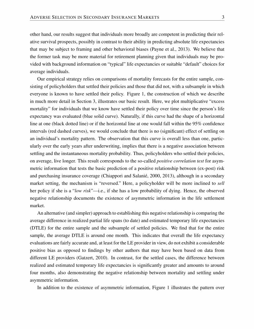
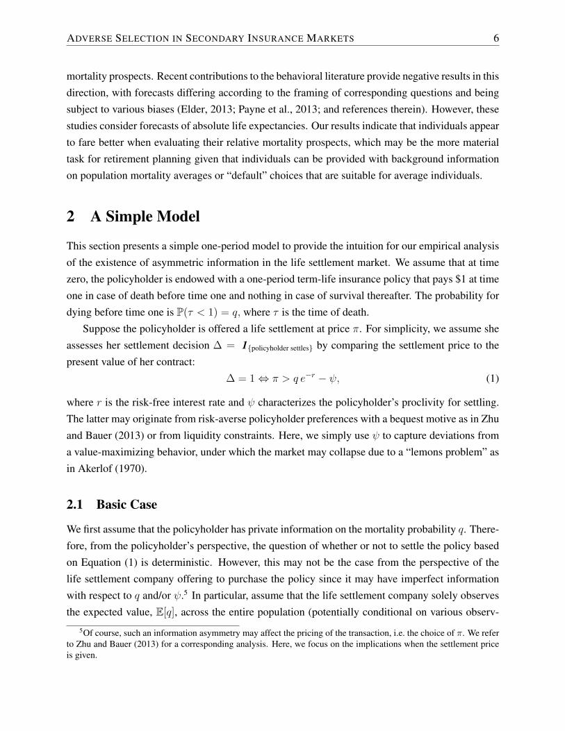
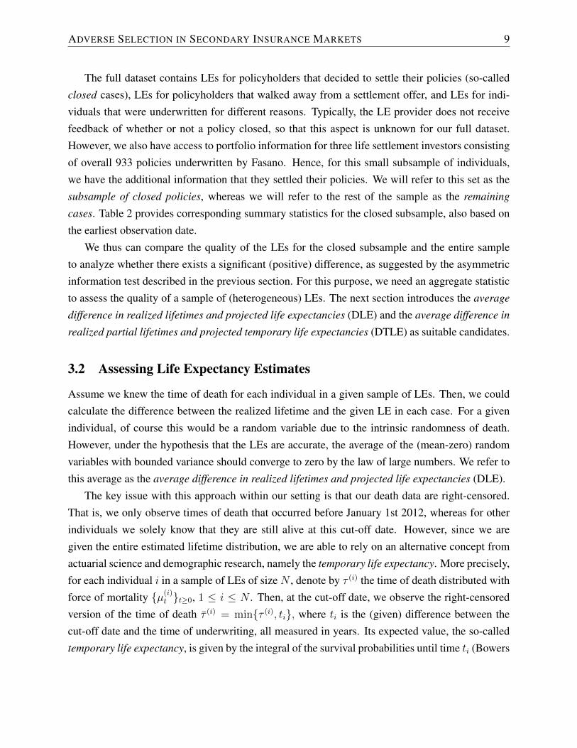
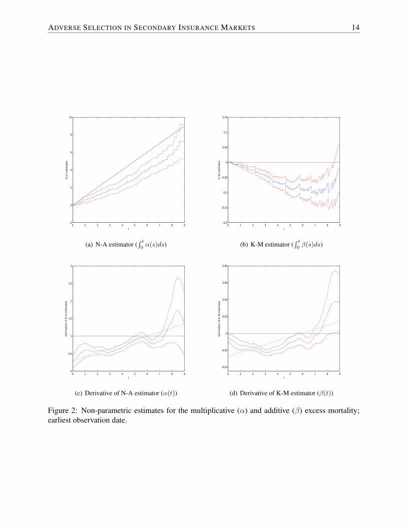
respectively.Figure 2 presents the results for the earliest observation date.8 More specifically, panels (a) and

(b) illustrate the N-A and the K-M estimate for the cumulative excess mortalities, including 95%confidence intervals. Panels (c) and (d) plot the corresponding excess mortality coefficients α andβ also including 95% confidence intervals, where we use the Epanechnikov kernel with a fixedbandwidth of one in their derivation.

In accordance with the results from the previous subsection, we find that the multiplicativeexcess mortality is mostly significantly less than one (panel (c)), i.e. individuals that settled theirpolicies on average live longer. This can also be inferred from the cumulative version (panel (a))that generally has a slope of less than one. Moreover, we observe a clear time pattern: The excessmortality in panel (c) is smallest right after underwriting but increases over time and is no longersignificantly different from zero after roughly five years. In other words, the impact of settling onthe policyholder’s force of mortality is temporary and wears off over time, until there is no longera significant effect after five to six years.

These findings are confirmed by the additive excess mortality, which also illustrates the nega-tive association between settling and mortality since it is overall significantly less than zero (panel(d)). A possible exception is the last observation year, where we see a slight positive effect, thoughthe overall effect on long-term survival probabilities is still negative since the cumulative mul-tiplicative excess mortality is less than zero (panel (b)).9 Moreover, we again generally find anincreasing trend over time with the impact wearing off and losing significance after five to sixyears. The observation that the trend over the first year appears to be negative while the multiplica-tive trend is increasing can be reconciled by the observation that the force of mortality is a rapidlyincreasing function.

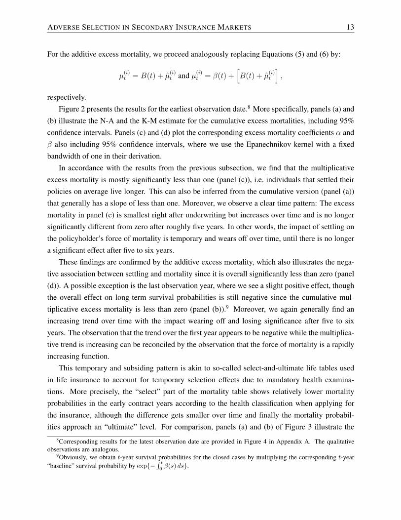
This temporary and subsiding pattern is akin to so-called select-and-ultimate life tables usedin life insurance to account for temporary selection effects due to mandatory health examina-tions. More precisely, the “select” part of the mortality table shows relatively lower mortalityprobabilities in the early contract years according to the health classification when applying forthe insurance, although the difference gets smaller over time and finally the mortality probabil-ities approach an “ultimate” level. For comparison, panels (a) and (b) of Figure 3 illustrate the

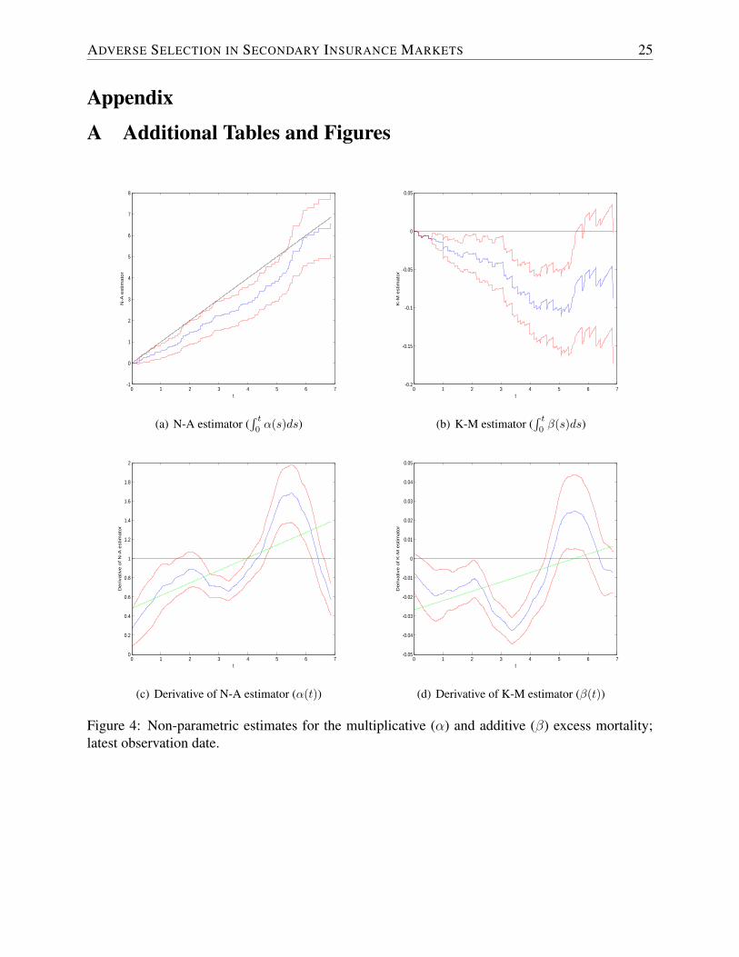
8Corresponding results for the latest observation date are provided in Figure 4 in Appendix A. The qualitativeobservations are analogous.

9Obviously, we obtain t-year survival probabilities for the closed cases by multiplying the corresponding t-year“baseline” survival probability by exp{−

∫ t

0β(s) ds}.


0 1 2 3 4 5 6 7 8 9-2

0

2

4

6

8

10

t

N-A

estim

ato

r

(a) N-A estimator (∫ t

0α(s)ds)

0 1 2 3 4 5 6 7 8 9-0.2

-0.15

-0.1

-0.05

0

0.05

0.1

0.15

t

K-M

estim

ato

r

(b) K-M estimator (∫ t

0β(s)ds)

0 1 2 3 4 5 6 7 8 90

0.5

1

1.5

2

2.5

3

t

Derivative o

f N

-A e

stim

ato

r

(c) Derivative of N-A estimator (α(t))

0 1 2 3 4 5 6 7 8 9

-0.04

-0.02

0

0.02

0.04

0.06

0.08

t

Derivative o

f K

-M e

stim

ato

r

(d) Derivative of K-M estimator (β(t))

Figure 2: Non-parametric estimates for the multiplicative (α) and additive (β) excess mortality;earliest observation date.


0 5 10 15 20 250

0.5

1

1.5

2

2.5

3

t

Excess m

ort

alit

y

(a) Multiplicative excess mortality

0 5 10 15 20 25

-0.04

-0.02

0

0.02

0.04

0.06

0.08

t

Excess m

ort

alit

y

(b) Additive excess mortality

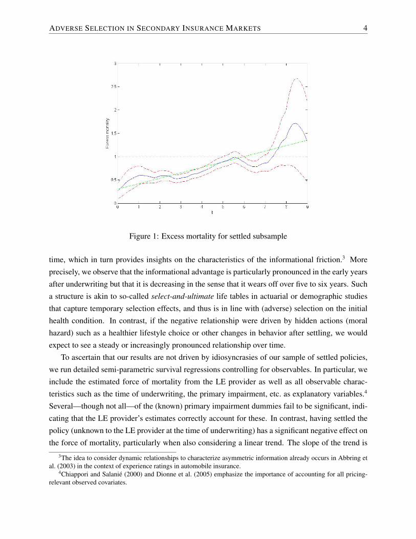
Figure 3: Excess mortality for the CSO 2001 preferred life table.

multiplicative and additive excess mortality after the life insurance underwriting process relativeto ultimate mortalities for a “preferred” 75-year old male according to the Commissioners Stan-

dard Ordinary (CSO) 2001 life table that is used for life insurance reserving according to USregulations. When comparing Figures 2 and 3, it is apparent that the overall structure is very sim-ilar, although the selection period due to mandatory health examinations in life insurance is muchlonger (around twenty years). In particular, we observe a steadily increasing multiplicative excessmortality whereas there is an initial reversal for the additive excess mortality due to the rapidlyincreasing property of the force of mortality.

This analogy suggests an informational advantage regarding the initial health condition thatindividuals select on in their settlement decision. If, in contrast, the difference in mortalities forpolicyholders that settled their policy were driven by hidden actions such as a change in behavioror lifestyle after settling, we would expect to see a persistent or even increasing impact on the forceof mortality. As such, the characteristics of the excess mortality are in line with adverse selectionrather than moral hazard—which is a second central result in this paper.

As previously indicated, the next section corroborates our results by running survival regres-sions that control for observables.


4 Survival Regression Analysis

When testing for asymmetric information in primary insurance markets, a common approach is toregress ex-post realized risk on ex-ante coverage as in (Cohen and Siegelman, 2010):

Riski = α + β ×Xi + γ × Coveragei + εi, (7)

where Xi is a vector of covariates observed by the insurer, and—ideally—by the econometrician.One can then infer the existence of asymmetric information if γ is significantly greater than zero,i.e. if there is a positive relationship between risk and purchase of coverage. As discussed in Section2, a corresponding prediction in secondary insurance markets is a negative relationship betweenrisk and settlement. Thus, in what follows, we test for asymmetric information by regressingex-post mortality risk on observables and the settlement decision.

4.1 Basic Specification

Since we observe right-censored survival data, conventional techniques based on linear (OLS)regression as for Equation (7) are not applicable. Instead, we rely on survival regression. However,in order to include the mortality estimate {µ(i)

t } by the LE provider as a covariate since it mayhave (additional) predictive power, conventional multiplicative specifications as within the Coxproportional hazard model are not feasible either. Thus, we rely on the following additive semi-parametric specification:

µ(i)t = β0(t)+β1 µ

(i)t +β2 DOUi+β3 AUi+β4 SEi+

15∑j=1

β5,j PIi,j +2∑j=1

β6,j SMi,j +γ1 SaOi. (8)

Here, DOUi is the underwriting date, measured in years and normalized so that zero correspondsto January 1st 2001—the starting date of our sample. AUi is the individual’s age at underwriting,measured in years. SEi is a sex dummy, zero for female and one for male. PIi,j, j = 1, . . . , 15,

are primary impairment dummies for various diseases.10 No dummy is activated for blank entries.SMi,j, j = 1, 2, are smoker dummies, where SMi,1 = 1 for smoker and SMi.2 = 1 for an “aggre-gate” entry. No dummy is activated for non-smokers. We omit information that is only availablefor a fraction of the individuals (states of residence, face amount). Finally, we include a settled-and-observed dummy SaOi that is set to one for the subsample of closed cases. Clearly, we test forasymmetric information by inferring whether γ1 is negative.

Semi-parametric additive regression models such as our specification (8) have been proposed

10We do not list the primary impairments to protect proprietary information of our data supplier since they are notmaterial to our results.


and discussed by Lin and Ying (1994), and they are special cases of the more general semi-parametric models considered by McKeague and Sasieni (1994) and the non-parametric additiveregression models by Aalen (1989). For its estimation, we rely on the generalized least-squaresapproach from Lin and Ying (1994), who also provide a formula for the log-likelihood value.

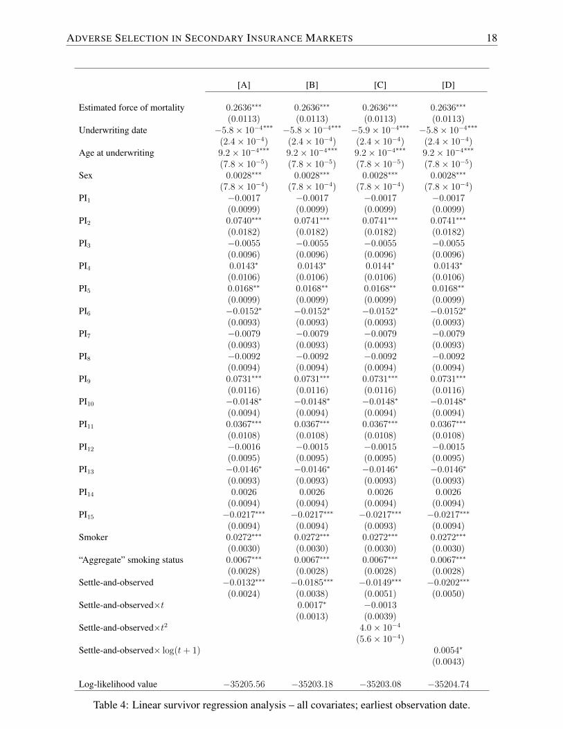
Column A in Table 4 presents the regression results for our basic model (8) and the earliest ob-servation date. We find that the estimated force of mortality is highly significant but the coefficientis considerably different from one, as one would expect in case of a perfect fit of the estimatesby the LE provider.11 In addition, various of the other characteristics are statistically significant,including the underwriting date, age, sex, smoking status, and some of the primary impairments.Note that this does not necessarily mean that the supplied estimates do not accurately account forthese covariates because the leading coefficient β1 is less than one.

As for the settled-and-observed covariate, the corresponding coefficient is negative and sig-nificant at the 99% level, i.e. individuals that settled have a lower mortality probability. Hence,again we find strong evidence for the existence of asymmetric information, also after controllingfor observables. This reinforces our conclusions from Section 3.

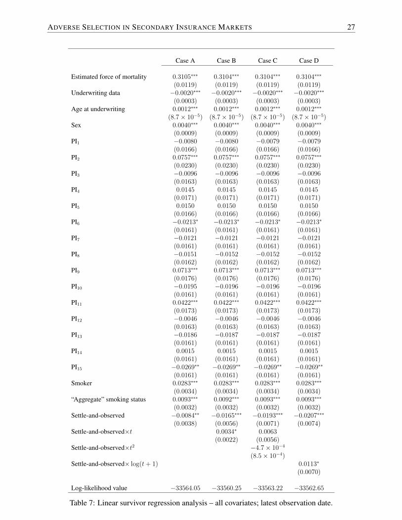
Column A of Table 6 in Appendix A provides results for an alternative specification in whichwe only keep the significant covariates. The result for the settlement decision remains unchanged.Moreover, we present corresponding results for the latest observation date in Table 7, also in Ap-pendix A. Again, the quantitative conclusions are identical.

4.2 Time Trend

To analyze the pattern of the excess mortality due to settling over time, we augment the basicspecification (8) by three different time trends: A basic linear trend [+γ2 SaOi t]; a quadratic trend[+γ2 SaOi t+ γ3 SaOi t

2]; and a logarithmic trend [+γ4 SaOi log{t+ 1}]. Columns B, C, and D inTable 4 display the results for the earliest observation date.12

The coefficients for the non-settlement related covariates remain essentially unchanged relativeto the basic specification. The basic settled-and-observed dummy again is negative and stronglysignificant in all cases. Moreover, we find that a basic linear trend is statistically significant at the90% level and notably increases the log-likelihood.13 In particular, the basic level γ1 decreases,

11As indicated in Footnote 6, this criterion may be too stringent since Fasano typically only supplies estimatedlife expectancies. As we show in the previous section, (temporary) life expectancy are relatively accurate. Also, thisassessment is based on the entire observation period and does not speak to the accuracy of current LEs. Additionalanalyses suggest that the quality was improving over time.

12Corresponding results for the latest observation date are provided in Appendix A. The quantitative conclusionsare again identical.

13Within our approach, parameters are obtained from a generalized least squares estimation procedure, so thatresults not necessarily coincide with maximum likelihood estimates as formally required for a likelihood ratio test.However, the test statistic would be significant at the 95% level.


[A] [B] [C] [D]

Estimated force of mortality 0.2636∗∗∗ 0.2636∗∗∗ 0.2636∗∗∗ 0.2636∗∗∗

(0.0113) (0.0113) (0.0113) (0.0113)Underwriting date −5.8× 10−4

∗∗∗ −5.8× 10−4∗∗∗ −5.9× 10−4

∗∗∗ −5.8× 10−4∗∗∗

(2.4× 10−4) (2.4× 10−4) (2.4× 10−4) (2.4× 10−4)Age at underwriting 9.2× 10−4

∗∗∗9.2× 10−4

∗∗∗9.2× 10−4

∗∗∗9.2× 10−4

∗∗∗

(7.8× 10−5) (7.8× 10−5) (7.8× 10−5) (7.8× 10−5)Sex 0.0028∗∗∗ 0.0028∗∗∗ 0.0028∗∗∗ 0.0028∗∗∗

(7.8× 10−4) (7.8× 10−4) (7.8× 10−4) (7.8× 10−4)PI1 −0.0017 −0.0017 −0.0017 −0.0017

(0.0099) (0.0099) (0.0099) (0.0099)PI2 0.0740∗∗∗ 0.0741∗∗∗ 0.0741∗∗∗ 0.0741∗∗∗

(0.0182) (0.0182) (0.0182) (0.0182)PI3 −0.0055 −0.0055 −0.0055 −0.0055

(0.0096) (0.0096) (0.0096) (0.0096)PI4 0.0143∗ 0.0143∗ 0.0144∗ 0.0143∗

(0.0106) (0.0106) (0.0106) (0.0106)PI5 0.0168∗∗ 0.0168∗∗ 0.0168∗∗ 0.0168∗∗

(0.0099) (0.0099) (0.0099) (0.0099)PI6 −0.0152∗ −0.0152∗ −0.0152∗ −0.0152∗

(0.0093) (0.0093) (0.0093) (0.0093)PI7 −0.0079 −0.0079 −0.0079 −0.0079

(0.0093) (0.0093) (0.0093) (0.0093)PI8 −0.0092 −0.0092 −0.0092 −0.0092

(0.0094) (0.0094) (0.0094) (0.0094)PI9 0.0731∗∗∗ 0.0731∗∗∗ 0.0731∗∗∗ 0.0731∗∗∗

(0.0116) (0.0116) (0.0116) (0.0116)PI10 −0.0148∗ −0.0148∗ −0.0148∗ −0.0148∗

(0.0094) (0.0094) (0.0094) (0.0094)PI11 0.0367∗∗∗ 0.0367∗∗∗ 0.0367∗∗∗ 0.0367∗∗∗

(0.0108) (0.0108) (0.0108) (0.0108)PI12 −0.0016 −0.0015 −0.0015 −0.0015

(0.0095) (0.0095) (0.0095) (0.0095)PI13 −0.0146∗ −0.0146∗ −0.0146∗ −0.0146∗

(0.0093) (0.0093) (0.0093) (0.0093)PI14 0.0026 0.0026 0.0026 0.0026

(0.0094) (0.0094) (0.0094) (0.0094)PI15 −0.0217∗∗∗ −0.0217∗∗∗ −0.0217∗∗∗ −0.0217∗∗∗

(0.0094) (0.0094) (0.0093) (0.0094)Smoker 0.0272∗∗∗ 0.0272∗∗∗ 0.0272∗∗∗ 0.0272∗∗∗

(0.0030) (0.0030) (0.0030) (0.0030)“Aggregate” smoking status 0.0067∗∗∗ 0.0067∗∗∗ 0.0067∗∗∗ 0.0067∗∗∗

(0.0028) (0.0028) (0.0028) (0.0028)Settle-and-observed −0.0132∗∗∗ −0.0185∗∗∗ −0.0149∗∗∗ −0.0202∗∗∗

(0.0024) (0.0038) (0.0051) (0.0050)Settle-and-observed×t 0.0017∗ −0.0013

(0.0013) (0.0039)Settle-and-observed×t2 4.0× 10−4

(5.6× 10−4)Settle-and-observed× log(t+ 1) 0.0054∗

(0.0043)

Log-likelihood value −35205.56 −35203.18 −35203.08 −35204.74

Table 4: Linear survivor regression analysis – all covariates; earliest observation date.


indicating a—relative to the baseline specification—stronger effect for mortalities immediatelyafter underwriting that wears off over time. Hence, our results are in line with the findings fromSection 3.3, where we discuss that such a pattern conforms with adverse selection on the initialhealth state.

Similarly, a logarithmic time trend is significant but yields a lower likelihood value. In contrast,the quadratic specification does not yield significant coefficients and only very slightly increasesthe likelihood value relative to the linear trend specification. The results for the settlement decisionremain unchanged.

4.3 Qualitative Impact

Of course we can rely on the regression coefficients γ1 and γ2 to derive an adjustment for survivalprobabilities—and, thus, life expectancies—for individuals in the closed subsample. However,this will not correspond to a suitable adjustment for closed cases relative to individuals that didnot settle their policies since, as detailed in Section 3.1, our remaining sample contains LEs forboth. Thus, it is necessary to inflate our estimates to account for the “commingled” nature of ourremaining sample of LEs, where of course the inflation rate depends on the total proportion ofsettled policies.

To illustrate and to derive the appropriate inflation rate, consider the following simplified ver-sion of our additive hazard model (8):

µ(i)t = β0(t) + γ1 SaOi.

Denote by Nt all (remaining) observations at time t, by N (1)t all (remaining) settled cases at time

t, pt = N(1)t /Nt, and by N

(2)t all (remaining) observed settled cases at time t, qt = N

(2)t /Nt.

Furthermore, denote by γOBS1 the unknown estimate for the model in which the econometricianobserves all settlement decisions, and by γACT1 the actual estimate based on observed cases only.Assume further that at any time t, the probability that a settlement decision is observed is a constantπ ∈ (0, 1]. Therefore, π N (1)

t = E(N(2)t ), and we have, based on the estimates in Lin and Ying

(1994):γOBS1

γACT1

=

∫ τ0N

(2)t [1− qt] dt∫ τ

0N

(2)t [1− pt] dt

,

which suggests thatγOBS1

γACT1

≈ (1− q)(1− p)

.

Here p is the overall proportion of settled cases and q is the overall proportion of observed settled

cases in the portfolio, which for simplicity we assume is constant. Thus, we are able to derive an


inflated version of the coefficient via:

γOBS1 = γACT1 × (1− q)(1− p)

, (9)

where of course γACT1 corresponds to the estimate from specification (8). In particular, since theratio (1− q)/(1− p) is always greater than one, the inflated coefficient will clearly be greater thanthe one estimated from the “commingled” sample.

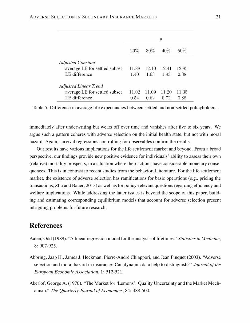
To illustrate the effect, we use Equation (9) to adjust our estimates from the previous subsec-tion, where we set q to 933/52, 603 according to the size of our closed subsample, and we usedifferent assumptions on p from 20% to 50%, according to rough guesses by our data supplier.Based on the adjusted estimates, we then derive life expectancies for a 75-year old US male pol-icyholder (cf. Table 1).14 In addition, we also calculate life expectancies for an adjusted versionof the specification with a linear trend, where we adjust γ1 according to (9) and γ2 such that theintersection with the time-axis remains the same, i.e. we assume the effect wears off over the sametime period.

Table 5 presents the results, where for comparison the non-adjusted life expectancy is 10.48years. The upper block provides calculations for the constant adjustment. We find that the impactof the adjustment is considerable, amounting to between 1.40 and 2.38 years, which corresponds tobetween 13% and 23% of the total life expectancy. In contrast, based on the adjusted linear trend,we obtain differences between 0.54 and 0.88 years, which still corresponds to between 5% and 8%of the life expectancy. These magnitudes suggest that adverse selection may have a considerableimpact on the life settlement market, and that asymmetric information should be accounted for inmarket operations and assessments.

5 Conclusion

In this paper, we provide evidence for asymmetric information in the life settlement market. Moreprecisely, we find that individuals that decided to settle their policies display significantly longer(temporary) lifetimes—as predicted by a basic model in which individuals have private informationon their mortality prospects. This finding is confirmed by survival regressions that control forobservable characteristics.

In addition, we derive non-parametric estimates of the excess mortality for individuals thatsettled as a function of time. We find that the difference is particularly pronounced in the years

14The mortality data are taken from the Human Mortality Database. University of California, Berkeley(USA), and Max Planck Institute for Demographic Research (Germany). Available at www.mortality.org orwww.humanmortality.de. More precisely, we calculate life expectancies based on expected future survival proba-bilities, where we use the Lee-Carter (Lee and Carter, 1992) method to produce forecasts.


p

20% 30% 40% 50%

Adjusted Constantaverage LE for settled subset 11.88 12.10 12.41 12.85LE difference 1.40 1.63 1.93 2.38

Adjusted Linear Trendaverage LE for settled subset 11.02 11.09 11.20 11.35LE difference 0.54 0.62 0.72 0.88

Table 5: Difference in average life expectancies between settled and non-settled policyholders.

immediately after underwriting but wears off over time and vanishes after five to six years. Weargue such a pattern coheres with adverse selection on the initial health state, but not with moralhazard. Again, survival regressions controlling for observables confirm the results.

Our results have various implications for the life settlement market and beyond. From a broadperspective, our findings provide new positive evidence for individuals’ ability to assess their own(relative) mortality prospects, in a situation where their actions have considerable monetary conse-quences. This is in contrast to recent studies from the behavioral literature. For the life settlementmarket, the existence of adverse selection has ramifications for basic operations (e.g., pricing thetransactions, Zhu and Bauer, 2013) as well as for policy-relevant questions regarding efficiency andwelfare implications. While addressing the latter issues is beyond the scope of this paper, build-ing and estimating corresponding equilibrium models that account for adverse selection presentintriguing problems for future research.

References

Aalen, Odd (1989). “A linear regression model for the analysis of lifetimes.” Statistics in Medicine,8: 907-925.

Abbring, Jaap H., James J. Heckman, Pierre-Andre Chiappori, and Jean Pinquet (2003). “Adverseselection and moral hazard in insurance: Can dynamic data help to distinguish?” Journal of the

European Economic Association, 1: 512-521.

Akerlof, George A. (1970). “The Market for ‘Lemons’: Quality Uncertainty and the Market Mech-anism.” The Quarterly Journal of Economics, 84: 488-500.


Andersen, Per Kragh, and Michael Vaeth (1989). “Simple parametric and nonparametric modelsfor excess and relative mortality.” Biometrics, 1989: 523-535.

Arrow, Kenneth J. (1963). “Uncertainty and the welfare economics of medical care.” American

Economic Review, 53: 941-973.

Billingsley, Patrick (1995). Probability and Measure, 3rd Edition, New York: John Wiley andSons.

Bowers, Newton L., Hans U. Gerber, James Hickman, Donald A. Jones, and Cecil J. Nesbitt(1997). Actuarial Mathematics, 2nd Edition, The Society of Actuaries.

Cardon, James H., and Igal Hendel (2001). “Asymmetric information in health insurance: evidencefrom the National Medical Expenditure Survey.” RAND Journal of Economics, 32: 408-427.

Cawley, John, and Tomas Philipson (1999). “An Empirical Examination of Information Barriersto Trade in Insurance.” American Economic Review, 89: 827-846.

Chiappori, Pierre-Andre, and Bernard Salanie (2000). “Testing for Asymmetric Information inInsurance Markets.” Journal of Political Economy, 108: 56-78.

Chiappori, Pierre-Andre, and Bernard Salanie (2013). “Asymmetric Information in Insurance Mar-kets: Predictions and Tests.” Handbook of Insurance, 2nd edition (G. Dionne, ed.). Springer,New York.

Cohen, Alma (2005). “Asymmetric Information and Learning in the Automobile Insurance Mar-ket.” Review of Economics and Statistics, 87: 197-207.

Cohen, Alma, and Liran Einav (2007). “Estimating risk preferences from deductible choice.”American Economic Review, 97: 74588.

Cohen, Alma, and Peter Siegelman (2010). “Testing for Adverse Selection in Insurance Markets.”Journal of Risk and Insurance, 77: 39-84.

Cutler, David M., Amy Finkelstein, and Kathleen McGarry (2008). “Preference Heterogeneityand Insurance Markets: Explaining a Puzzle of Insurance.” American Economic Review, 98:157-162.

Daily, Glenn, Igal Hendel, and Alessandro Lizzeri (2008). “Does the Secondary Life InsuranceMarket Threaten Dynamic Insurance?” American Economic Review, 98: 151-156.


Dionne, Georges, Mathieu Maurice, Jean Pinquet, and Charles Vanasse (2005). “The Role ofMemory in Long-Term Contracting with Moral Hazard: Empirical Evidence in AutomobileInsurance.” Working Paper.

Einav, Lian, Amy Finkelstein, and Paul Schrimpf (2007). “The welfare cost of asymmetric infor-mation: evidence from the U.K. annuity market.” NBER Working Paper No. 13228.

Einav, Lian, Amy Finkelstein, and Paul Schrimpf (2010)a. “Optimal Mandates and the WelfareCost of Asymmetric Information: Evidence from the U.K. Annuity Market.” Econometrica, 78:1031-1092.

Einav, Lian, Amy Finkelstein, and Jonathan Levin (2010)b. “Beyond Testing: Empirical Modelsof Insurance Markets.” Annual Review of Economics, 2: 311-336.

Elder, Todd E. (2013). “The Predictive Validity of Subjective Mortality Expectations: EvidenceFrom the Health and Retirement Study.” Demography, 50: 569-589.

Fang, Hanming, Michael P. Keane, and Dan Silverman (2008). “Sources of Advantageous Se-lection: Evidence from the Medigap Insurance Market.” Journal of Political Economy, 116:303-350.

Fang, Hanming, and Edward Kung (2010). “How Does Life Settlement Affect the Primary LifeInsurance Market?” NBER Working Paper No. 15761.

Finkelstein, Amy, and Kathleen McGarry (2006). “Multiple dimensions of private information:evidence from the long-term care insurance market.” American Economic Review, 96: 938-958.

Finkelstein, Amy, and James Poterba (2002). “Selection effects in the United Kingdom individualannuities market.” The Economic Journal, 112: 2850.

Finkelstein, Amy, and James Poterba (2004). “Adverse Selection in Insurance Markets: Policy-holder Evidence from the U.K. Annuity Market.” Journal of Political Economy, 112: 183-208.

Gatzert, Nadine (2010). “The Secondary Market for Life Insurance in the U.K., Germany, and theU.S.: Comparison and Overview.” Risk Management and Insurance Review, 13: 279-301.

Granieri, Vincent J., and Gregory P. Heck (2013). “Survival Characteristics of Three Senior Pop-ulations, with a Focus on Life Settlements.” Paper presented at the SOA Living to 100 andBeyond Symposium.

He, Daifeng (2009). “The life insurance market: Asymmetric information revisited.” Journal of

Public Economics, 93: 1090-1097.


Lee, Ronald D., and Lawrence R. Carter (1992). “Modeling and Forecasting U. S. Mortality.”Journal of the American Statistical Association, 87: 659-675.

Lin, D.Y., and Zhiliang Ying (1994). “Semiparametric analysis of the additive risk model.”Biometrika, 81: 61-71.

McCarthy, David, and Olivia S. Mitchell (2010). “International adverse selection in life insuranceand annuities.” Ageing in Advanced Industrial States, Springer Netherlands, 119-135.

McKeague, Ian W., and Peter D. Sasieni (1994). “A partly parametric additive risk model.”Biometrika, 81: 501-514.

Payne, John W., Namika Sagara, Suzanne B. Shu, Kirstin C. Appelt, and Eric J. Johnson (2013).“Life expectancy as a constructed belief: Evidence of a live-to or die-by framing effect.” Journal

of Risk and Uncertainty, 46: 27-50.

Puelz, Robert, and Arthur Snow (1994). “Evidence on adverse selection: Equilibrium signalingand cross-subsidization in the insurance market.” Journal of Political Economy, 102: 236-257.

Rothschild, Michael, and Joseph Stiglitz (1976). “Equilibrium in competitive insurance markets:An essay on the economics of imperfect information.” The Quarterly Journal of Economics, 90:630-649.

Wang, Jane-Ling (2005). “Smoothing Hazard Rates.” Encyclopedia of Biostatistics, 2005.

Wu, Xi, and Li Gan (2013). “Multiple Dimensions of Private Information in Life Insurance Mar-kets.” NBER Working Paper No. 19629.

Zhu, Nan, and Daniel Bauer (2011). “On the Economics of Life Settlements.” Proceedings of theRisk Theory Society – 2011.

Zhu, Nan, and Daniel Bauer (2013). “Coherent Pricing of Life Settlements Under AsymmetricInformation.” Journal of Risk and Insurance, 80: 827-851.


Appendix

A Additional Tables and Figures

0 1 2 3 4 5 6 7-1

0

1

2

3

4

5

6

7

8

t

N-A

estim

ato

r

(a) N-A estimator (∫ t

0α(s)ds)

0 1 2 3 4 5 6 7-0.2

-0.15

-0.1

-0.05

0

0.05

tK

-M e

stim

ato

r

(b) K-M estimator (∫ t

0β(s)ds)

0 1 2 3 4 5 6 70

0.2

0.4

0.6

0.8

1

1.2

1.4

1.6

1.8

2

t

Derivative o

f N

-A e

stim

ato

r

(c) Derivative of N-A estimator (α(t))

0 1 2 3 4 5 6 7-0.05

-0.04

-0.03

-0.02

-0.01

0

0.01

0.02

0.03

0.04

0.05

t

Derivative o

f K

-M e

stim

ato

r

(d) Derivative of K-M estimator (β(t))

Figure 4: Non-parametric estimates for the multiplicative (α) and additive (β) excess mortality;latest observation date.


Case A Case B Case C Case D


(0.0113) (0.0113) (0.0113) (0.0113)Underwriting date −5.5× 10−4

∗∗ −5.5× 10−4∗∗ −5.5× 10−4

∗∗ −5.5× 10−4∗∗

(2.4× 10−4) (2.4× 10−4) (2.4× 10−4) (2.4× 10−4)Age at underwriting 9.1× 10−4

∗∗∗9.1× 10−4

∗∗∗9.1× 10−4

∗∗∗9.1× 10−4

∗∗∗

(7.9× 10−5) (7.9× 10−5) (7.9× 10−5) (7.9× 10−5)Sex 0.0027∗∗∗ 0.0027∗∗∗ 0.0027∗∗∗ 0.0027∗∗∗

(7.7× 10−4) (7.7× 10−4) (7.7× 10−4) (7.7× 10−4)PI2 0.0780∗∗∗ 0.0780∗∗∗ 0.0780∗∗∗ 0.0780∗∗∗

(0.0157) (0.0157) (0.0157) (0.0157)PI4 0.0184∗∗∗ 0.0184∗∗∗ 0.0184∗∗∗ 0.0184∗∗∗

(0.0053) (0.0053) (0.0053) (0.0053)PI5 0.0209∗∗∗ 0.0209∗∗∗ 0.0209∗∗∗ 0.0209∗∗∗

(0.0037) (0.0037) (0.0037) (0.0037)PI6 −0.0110∗∗∗ −0.0110∗∗∗ −0.0110∗∗∗ −0.0110∗∗∗

(0.0011) (0.0011) (0.0011) (0.0011)PI9 0.0773∗∗∗ 0.0773∗∗∗ 0.0773∗∗∗ 0.0773∗∗∗

(0.0071) (0.0071) (0.0071) (0.0071)PI10 −0.0106∗∗∗ −0.0106∗∗∗ −0.0106∗∗∗ −0.0106∗∗∗

(0.0014) (0.0014) (0.0014) (0.0014)PI11 0.0408∗∗∗ 0.0408∗∗∗ 0.0408∗∗∗ 0.0408∗∗∗

(0.0056) (0.0056) (0.0056) (0.0056)PI13 −0.0104∗∗∗ −0.0104∗∗∗ −0.0104∗∗∗ −0.0104∗∗∗

(9.2× 10−4) (9.2× 10−4) (9.2× 10−4) (9.2× 10−4)PI15 −0.0175∗∗∗ −0.0175∗∗∗ −0.0175∗∗∗ −0.0175∗∗∗

(8.4× 10−4) (8.4× 10−4) (8.4× 10−4) (8.4× 10−4)Smoker 0.0279∗∗∗ 0.0279∗∗∗ 0.0279∗∗∗ 0.0279∗∗∗


(0.0028) (0.0028) (0.0028) (0.0028)Settle-and-observed −0.0131∗∗∗ −0.0185∗∗∗ −0.0149∗∗∗ −0.0202∗∗∗

(0.0024) (0.0038) (0.0051) (0.0050)Settle-and-observed×t 0.0017∗ −0.0013

(0.0013) (0.0039)Settle-and-observed×t2 4.0× 10−4


(0.0043)


Table 6: Linear survivor regression analysis – reduced covariates, earliest observation date.


Case A Case B Case C Case D


(0.0119) (0.0119) (0.0119) (0.0119)Underwriting data −0.0020∗∗∗ −0.0020∗∗∗ −0.0020∗∗∗ −0.0020∗∗∗

(0.0003) (0.0003) (0.0003) (0.0003)Age at underwriting 0.0012∗∗∗ 0.0012∗∗∗ 0.0012∗∗∗ 0.0012∗∗∗

(8.7× 10−5) (8.7× 10−5) (8.7× 10−5) (8.7× 10−5)Sex 0.0040∗∗∗ 0.0040∗∗∗ 0.0040∗∗∗ 0.0040∗∗∗

(0.0009) (0.0009) (0.0009) (0.0009)PI1 −0.0080 −0.0080 −0.0079 −0.0079

(0.0166) (0.0166) (0.0166) (0.0166)PI2 0.0757∗∗∗ 0.0757∗∗∗ 0.0757∗∗∗ 0.0757∗∗∗

(0.0230) (0.0230) (0.0230) (0.0230)PI3 −0.0096 −0.0096 −0.0096 −0.0096

(0.0163) (0.0163) (0.0163) (0.0163)PI4 0.0145 0.0145 0.0145 0.0145

(0.0171) (0.0171) (0.0171) (0.0171)PI5 0.0150 0.0150 0.0150 0.0150

(0.0166) (0.0166) (0.0166) (0.0166)PI6 −0.0213∗ −0.0213∗ −0.0213∗ −0.0213∗

(0.0161) (0.0161) (0.0161) (0.0161)PI7 −0.0121 −0.0121 −0.0121 −0.0121

(0.0161) (0.0161) (0.0161) (0.0161)PI8 −0.0151 −0.0152 −0.0152 −0.0152

(0.0162) (0.0162) (0.0162) (0.0162)PI9 0.0713∗∗∗ 0.0713∗∗∗ 0.0713∗∗∗ 0.0713∗∗∗

(0.0176) (0.0176) (0.0176) (0.0176)PI10 −0.0195 −0.0196 −0.0196 −0.0196

(0.0161) (0.0161) (0.0161) (0.0161)PI11 0.0422∗∗∗ 0.0422∗∗∗ 0.0422∗∗∗ 0.0422∗∗∗

(0.0173) (0.0173) (0.0173) (0.0173)PI12 −0.0046 −0.0046 −0.0046 −0.0046

(0.0163) (0.0163) (0.0163) (0.0163)PI13 −0.0186 −0.0187 −0.0187 −0.0187

(0.0161) (0.0161) (0.0161) (0.0161)PI14 0.0015 0.0015 0.0015 0.0015

(0.0161) (0.0161) (0.0161) (0.0161)PI15 −0.0269∗∗ −0.0269∗∗ −0.0269∗∗ −0.0269∗∗

(0.0161) (0.0161) (0.0161) (0.0161)Smoker 0.0283∗∗∗ 0.0283∗∗∗ 0.0283∗∗∗ 0.0283∗∗∗


(0.0032) (0.0032) (0.0032) (0.0032)Settle-and-observed −0.0084∗∗ −0.0165∗∗∗ −0.0193∗∗∗ −0.0207∗∗∗

(0.0038) (0.0056) (0.0071) (0.0074)Settle-and-observed×t 0.0034∗ 0.0063

(0.0022) (0.0056)Settle-and-observed×t2 −4.7× 10−4


(0.0070)


Table 7: Linear survivor regression analysis – all covariates; latest observation date.

Documents

Adverse Selection in Secondary Insurance Markets: … · Adverse Selection in Secondary Insurance Markets: Evidence from the Life ... although in a secondary market ... for the settled