Embed Size (px)
Citation preview
Advertising and Demand for Addictive Goods:The Effects of E-Cigarette Advertising
Anna E. Tuchman∗
June 26, 2015
Job Market PaperPRELIMINARY AND IN PROGRESS
Current Version: http://stanford.edu/∼tuchman
AbstractAlthough TV advertising for traditional cigarettes has been banned since 1971, adver-
tising for electronic cigarettes remains unregulated. The effects of e-cigarette ads havebeen heavily debated by policymakers and the media, though empirical analysis of themarket has been limited. To analyze the question, I leverage access to county-level sales andadvertising data on cigarettes and related tobacco products, along with detailed data on theconsumption behavior of a panel of households. I exploit a discontinuity in advertising alongtelevision market borders to present descriptive evidence that suggests that e-cigarette adver-tising reduces aggregate demand for traditional cigarettes. Analyzing household purchasedata, I find that individuals reduce their consumption of traditional cigarettes after buyinge-cigarettes, further suggesting that the products are substitutes. I then specify a structuralmodel of demand for cigarettes that incorporates addiction and allows for heterogeneityacross households. The model enables me to leverage the information content of bothdatasets to identify variation in tastes across markets and the state dependence inducedon choice by addiction. I show how the model can be estimated linking both datasets in aunified estimation procedure. Using the demand model estimates, I evaluate the impact ofa proposed ban on e-cigarette television advertising. I find that in the absence of e-cigaretteadvertising, demand for traditional cigarettes would increase, suggesting that a ban one-cigarette advertising may have unintended consequences.
∗Doctoral Student in Marketing, Stanford Graduate School of Business, Email: [email protected]. I amgrateful to my advisor, Harikesh Nair, and my committee, Wes Hartmann and Navdeep Sahni, for their guidanceand support. Thanks also to Kristina Brecko, Øystein Daljord, Pedro Gardete, James Lattin, Sridhar Narayanan,Wonhee Park, Stephan Seiler, Breno Vieira, and the participants at the Stanford IO and Marketing seminars. Ithank the Kilts Center for Marketing and the Americans for Nonsmokers’ Rights Foundation for their help withdata resources. All remaining errors are my own.
1
1 Introduction
Smoking cigarettes is still the leading cause of preventable death in the United States, killing
more than 480,000 people a year. As a result, cigarette advertising remains a public health
issue that is intensely debated by cigarette companies, policy makers, and academic researchers.
Although all TV and radio advertising for traditional cigarettes has been banned since 1971,
attention to the advertising ban has been renewed by the entry of e-cigarettes into the market.
E-cigarettes first entered the US market in 2007 and quickly grew to become a $2 billion industry
by 2014 (Crowley (2015)). E-cigarette advertising does not fall under the tobacco advertising
ban and thus remains unregulated. Advertising for e-cigarettes has proliferated in recent years
on television, online, and in print media outlets. By 2013, e-cigarette marketing spending
exceeded $79 million with the majority of spending going towards TV advertising (Kantar
Media (2014)). Activists advocating for a ban on e-cigarette advertising argue that e-cigarette
ads glamorize smoking and that e-cigarettes may act as a gate-way into smoking traditional
cigarettes and marijuana. Proponents of e-cigarettes argue that e-cigarettes may be used as a
tool to effectively help quit smoking. To date, there exists little empirical evidence in support of
either of these positions.
In this paper, I use data through 2012 to empirically test whether e-cigarette advertising
increases or decreases demand for traditional cigarettes and consider the implications of
proposals to ban e-cigarette advertising. I use both descriptive and structural methods to
analyze this issue and find that e-cigarette advertising reduces demand for traditional cigarettes.
At current levels of advertising, my counterfactual analysis predicts a 3% increase in cigarette
demand as a result of an e-cigarette advertising ban.1 This is an economically significant
increase that is comparable in magnitude to the decrease in overall smoking prevalence in the
US between 2010 and 2011.
Although the market for e-cigarettes is still small relative to tobacco cigarettes, awareness
and use of e-cigarettes has been growing steadily in recent years. Giovenco et al. (2014)
surveyed a random sample of current and former smokers in June 2013 and found that almost
half (47%) of respondents had tried an e-cigarette product at least once, though only 4% of
respondents reported established use.2 Despite being a quickly growing sector in a controversial
1These numbers may be revised as the model is updated and new data is incorporated.2Established use defined as having used an e-cigarette product more than 50 times.
2

industry, much is still unknown about e-cigarettes to date because the category is still new.
Existing research relating to e-cigarettes has generally been focused on addressing three types of
questions: i) what are the health effects of e-cigarettes to users and non-users, ii) are e-cigarettes
an effective tool to help smokers quit smoking, and iii) do e-cigarettes hamper existing tobacco
control efforts. This paper primarily relates to the third category.
In general, whether e-cigarettes have a positive or negative impact on public health
and tobacco control depends on the interplay between the potential benefits to be derived
by current smokers and the undesired adoption of nicotine products by non-smokers. The
World Health Organization’s 2014 report on electronic nicotine delivery systems discusses the
two primary arguments made by advocates for a ban on e-cigarette advertising: the gateway
and renormalization effects (WHO (2014)). The gateway effect refers to the possibility that
e-cigarettes will cause non-smokers to initiate nicotine use at a higher rate than they would
if e-cigarettes did not exist and that once addicted to nicotine, non-smokers will be more
likely to switch to smoking cigarettes than they would if they were not e-cigarette users. The
renormalization effect refers to the possibility that marketing that portrays e-cigarettes as an
attractive product will increase the attractiveness of cigarettes as well. The WHO (2014) report
acknowledges that the existence and magnitude of the gateway and renormalization effects is
an empirical question that is still understudied due to the limited availability of data.
Advocates for a ban on e-cigarette advertising often bring up both the gateway and
renormalization effects in the context of teen consumption, as teens have rapidly increased
their use of e-cigarettes in recent years. The 2014 National Youth Tobacco Survey found that for
the first time, middle and high school students used e-cigarettes more than any other tobacco
product, including conventional cigarettes. However, overall middle and high school students
did not increase their overall tobacco use between 2011 and 2014; the increase in e-cigarette
use was offset by a decline in traditional cigarette and cigar use. Still, researchers are concerned
about the long-term consequences of teenagers adopting e-cigarettes since surveys indicate that
about 90% of current smokers first tried cigarettes as teens and that about 75% of teen smokers
continue to smoke as adults (2012 Surgeon General’s Report). My ability to study the important
question of youth adoption of e-cigarettes is unfortunately limited by the short window of data
available on the nascent industry. Although this paper does not address the long-run effects of
youth adoption, it contributes to our basic understanding of the balance between the positive
and negative effects of e-cigarette advertising.
3
To my knowledge, this paper provides the first empirical analysis of the effects of e-
cigarette advertising on demand for traditional cigarettes and e-cigarettes. First, I use store
sales data and local advertising data to determine whether e-cigarette advertising increases
or decreases demand for cigarettes. Identifying advertising effects can be challenging and is
the focus of a large body of academic research. Randomization and instrumental variables are
tools frequently used by researchers to identify causal effects of advertising. My strategy for
identifying advertising effects is a hybrid regression discontinuity differences in differences
approach based on the important recent work of Shapiro (2014), and similar to the identification
approaches taken by Card & Krueger (1994) and Black (1999). The idea is to take advantage
of discontinuities in television market borders that lead similar individuals to be exposed to
different levels of advertising. In this way, each border discontinuity can be thought of as a
natural experiment through which we can learn about the causal effect of advertising.
I present difference-in-differences regressions which indicate that e-cigarette advertising
increases demand for e-cigarettes and decreases demand for traditional cigarettes. After
identifying advertising effects in the aggregate data, I use household purchase panel data to
document the substitution patterns between e-cigarettes and traditional cigarettes. Household
purchase patterns indicate that e-cigarettes are a substitute to traditional cigarettes. The
household data also reveals a pattern of addiction; current period demand for cigarettes is
increasing in past consumption.
Finally, to quantify the effects of a proposed ban on e-cigarette advertising, I construct
and estimate a model of demand for cigarettes that allows me to leverage the virtues of both
aggregate and household data. The demand model aggregates in an internally consistent way,
such that equations governing household and aggregate demand are functions of the same
underlying structural parameters. The model enables me to utilize the information content of
the two datasets in a unified way to identify the two main primitives of interest - heterogeneity
in tastes for products and advertising, and the persistence in choices generated by addiction. I
show how the discontinuities I exploit in the linear descriptive models port to the more complex,
nonlinear structural model in an intuitive way, thus showing in a transparent manner how
to leverage the same identification in all model specifications. I estimate the model using an
integrated procedure proposed by Chintagunta & Dubé (2005) that recovers mean utility levels
and unobserved demand shocks from the aggregate data and identifies parameters governing
addiction and heterogeneity off of the household purchase data. I then use the estimated model
4

parameters to predict the impact of a ban on e-cigarette advertising and other alternative policy
interventions.
My research contributes to the ongoing policy debate as to whether e-cigarette TV
advertising should be banned and suggests that a ban on e-cigarette advertising may have
unintended consequences. More generally, my approach contributes to the study of advertising
in categories with state dependence and to the analysis of substitution and complementarities
in demand across categories.
In the sections that follow, I review the existing literature on addiction and cigarette
advertising and describe the industry context in more detail. Next I discuss my identification
strategy and present descriptive analyses of aggregate and household-level purchase data.
Motivated by these results, the second half of the paper introduces a demand model for
cigarettes and describes an integrated estimation procedure that utilizes both the aggregate
and household data. I then use the demand estimates in a counterfactual analysis to predict
the impact on cigarette demand of a ban on e-cigarette TV advertising. Finally, I conclude the
paper by summarizing the key findings and outlining directions for future research.
2 Literature Review
My research is primarily related to the literatures on addiction and advertising in the cigarette
industry. In the sections below I discuss the existing work in these areas and how it relates to
my research.
2.1 Addiction
A large body of literature in economics and marketing has analyzed markets for addictive goods.
In classic models of addiction, a good is considered to be addictive if past consumption of the
good raises the marginal utility of present consumption. There are generally two classes of
economic models of addiction: myopic models and models with forward-looking consumers.
Myopic models allow past consumption to affect current consumption decisions, but assume
that consumers are not forward-looking about the fact that their consumption in the current
period will affect their utility from consumption in future periods. Researchers have empirically
tested for addiction in the cigarette market and found strong evidence that current consumption
is increasing in past consumption (Houthakker & Taylor (1970), Mullahy (1985)). In myopic
5

models of addiction, increases in current and past prices will reduce current consumption
(Baltagi & Levin (1986), Jones (1989)), but increases in future prices will not affect current
consumption. On the other hand, in the “rational addiction” model, forward-looking consumers
consider the future implications of addictive consumption when making consumption decisions
in the current period (Becker & Murphy (1988), Gordon & Sun (2014)). Consistent with the
rational addiction model, empirical studies have found evidence that consumers reduce their
consumption in the current period in response to increases in past, current, and expected
future prices (Pashardes (1986), Chaloupka (1991), Becker et al. (1994)). However, many
researchers object to the perfect foresight assumption of the rational addiction model (Winston
(1980), Akerlof (1991)). In response to these concerns, researchers have attempted to address
perceived inconsistencies in the perfect foresight assumption by allowing for learning and
bounded-rationality (Orphanides & Zervos (1995), Suranovic et al. (1999)).
Many empiricists have applied myopic and forward-looking models of addiction to data
in order to measure the responsiveness of demand for addictive goods to changes in price.
Researchers have found that temporary price changes for addictive goods have little impact on
demand. However, long-run responses to permanent price increases are substantially larger
than short-run reductions in demand (Chaloupka & Warner (1999)). These results suggest
that ignoring the addictive nature of demand for tobacco and other drugs will lead to biased
predictions of long-run responses to price changes.
In my analysis, I present a myopic model of cigarette addiction in which past consumption
is complementary to current consumption. I do not model rational addiction in the sense that
individuals in my model are not forward-looking. I think this assumption is reasonable given
that e-cigarettes at the time were a new product with highly uncertain future quality and price.
2.2 Cigarette Advertising
My analysis is closely related to research measuring the effects of cigarette advertising on
demand for cigarettes. In particular, a large stream of research has focused on measuring the
effects of the 1971 ban on cigarette TV advertising (Ippolito et al. (1979), Schneider et al.
(1981), Porter (1986), Baltagi & Levin (1986), Kao & Tremblay (1998), McAuliffe (1988),
Seldon & Doroodian (1989), Franke (1994)). Despite extensive work in the area, research
has produced mixed results. Many studies conclude that the ban did not significantly reduce
cigarette consumption, while others have found evidence that the marginal productivity of
6
cigarette advertising fell after the ban (Tremblay & Tremblay (1995)). Schneider et al. (1981)
provides empirical evidence showing that the advertising ban led to a 5% net increase in per
capita tobacco consumption as a result of price reductions resulting from cutting advertising
costs. Researchers have pointed to but not resolved the potential endogeneity of advertising and
advertising regulation, as well as firms’ ability to substitute advertising to other media as factors
that have complicated empirical analyses of the effects of the advertising ban (Saffer (1998),
Stewart (1993)). Other papers have focused on analyzing firms’ responses to the advertising
ban. Eckard (1991) focuses on the effects of the ban on competition between firms and industry
concentration while Qi (2013) explains the increase in total industry ad spending after the ban
as a combination of dynamic competition and firms learning about ad effectiveness.
My work primarily relates to the stream of papers that seek to measure the effects of
advertising regulation on cigarette demand. While the majority of these studies were limited
to using data on aggregate advertising expenditures, I am able to address the endogeneity of
advertising using detailed weekly, market-level data on advertising intensity and an identification
strategy which exploits across-market variation in advertising over time. As I currently do not
model the supply side of the market, my analysis will not capture firms’ strategic responses to a
potential ban on e-cigarette television advertising of the type considered by Eckard (1991) and
Qi (2013).
In the marketing literature, a recent paper by Wang et al. (2015) studies countermar-
keting strategies including excise taxes, smoke-free restrictions, and antismoking advertising
campaigns and compares the effects of these policy levers to the effects of print advertising for
cigarette products. My work is related to the extent that e-cigarette advertising is another tool
that can be used to shift demand for traditional cigarettes.
2.3 E-Cigarette Advertising and Demand
Existing empirical analysis of the e-cigarette industry has reported basic statistics on advertising
exposure and calculated price elasticities using aggregate data. Duke et al. (2014) document
the increase in youth and young adult exposure to e-cigarette advertising, but they do not link
this advertising exposure to purchase outcomes. Huang et al. (2014) use quarterly market-
level data and fixed effects regressions to measure the own- and cross-price elasticities of
e-cigarettes and traditional cigarettes. The authors estimate price elasticities for e-cigarettes
between -1.2 and -1.9 and positive but not statistically significant cross-price elasticities between
7

e-cigarettes and traditional cigarettes. They find elasticities for e-cigarettes that are 2-3 times
higher than elasticities that have been estimated for traditional cigarettes. My research builds
on this descriptive analysis of the e-cigarette industry and considers the effects of e-cigarette
advertising on demand for traditional and electronic cigarettes.
3 Empirical Setting
3.1 Tobacco Advertising Ban
The Surgeon General released its groundbreaking report linking smoking to lung cancer and
increased mortality in 1964. Soon after, Congress passed the Federal Cigarette Labeling and
Advertising Act of 1965 which required a health warning label on all cigarette packages. Despite
the increased awareness about the negative health effects of smoking that was generated by
these interventions, cigarettes remained one of the most advertised products on TV. Under
pressure to reduce youth exposure to cigarette ads, in 1969 Congress approved the Public
Health Cigarette Smoking Act, which banned all advertising for cigarettes on any medium
of electronic communication subject to the jurisdiction of the FCC. The legislation effectively
prohibited cigarette advertising on TV and radio. The ban went into effect on January 1, 1971,
and is still in effect today.
Despite this restriction, cigarette companies continue to market their product aggressively.
The FTC reports that in 2012 the major cigarette manufacturers spent $9.168 billion on cigarette
advertising and promotion (FTC (2015)). The majority of cigarette marketing spending comes
in the form of promotional allowance, a category which includes price discounts and payments
made to retailers and wholesalers to facilitate the sale or placement of cigarettes. Price discounts
paid to cigarette retailers and wholesalers to reduce the price of cigarettes to consumers make
up the largest share (85%) of marketing spending in 2012 with a total of $7.802 billion.
Promotional allowances paid to retailers to facilitate the sale or placement of cigarettes and
incentive payments given to wholesalers accounted for another 8% of cigarette marketing
spending. The remaining spending was distributed across the following categories: coupons
(2.6%), adult-only public entertainment (1.2%), point-of-sale advertising (0.7%), direct mail
advertising (0.5%), magazine advertising (0.3%), online advertising (0.2%) and outdoor
advertising (0.03%).
8
3.2 E-Cigarettes
In 2004, the Chinese company Ruyan introduced the world’s first e-cigarette. The product
entered the US market soon after in 2007. An e-cigarette is an electronic device that contains
a nicotine-based liquid. When heated, the liquid becomes a vapor which the user inhales. E-
cigarettes do not contain tobacco and do not produce smoke because they do not use combustion.
There are two main variants of e-cigarettes – a durable, re-usable product that can be recharged
with included batteries and refilled with replacement cartridges, and a disposable product.
Many e-cigarette companies sell both a refillable and a disposable device. Although e-cigarettes
vary greatly in appearance, the most popular brands bear a close physical resemblance to
traditional cigarettes. E-cigarettes are available in many flavor varieties including tobacco,
cotton candy, and bubble gum. Opponents to e-cigarettes argue that these flavors increase the
product’s attractiveness to youth.
Until early 2012, the e-cigarette market was composed of many small independent
brands. In April 2012, Lorillard (the 3rd largest US tobacco company) acquired Blu eCigs for
$135 million. They became the first of the Big Tobacco companies to enter the e-cigarette
market. Reynolds (the 2nd largest US tobacco company, now merged with Lorillard) launched
its own brand Vuse in July 2013. Altria (the largest US tobacco company) launched its own
brand, MarkTen, in August 2013.
To date, the federal government has taken minimal steps to regulate e-cigarettes. E-
cigarettes are sold in retail stores and online and are not federally taxed as are traditional
tobacco cigarettes. Currently, minimum purchase age restrictions are determined by state
governments, but the FDA has recently proposed regulation that would instate 18 as a national
minimum age to purchase e-cigarettes. The FDA has also raised concerns about the lack of
quality control and consumer protection standards. The low barriers of entry have led to a
proliferation of hundreds of firms in the industry.
With the increasing popularity of e-cigarettes, a growing body of literature has developed
around studying the health effects of e-cigarette use and second-hand exposure. The long-term
health effects of e-cigarettes are still being investigated by clinical researchers, but initial studies
seem to indicate that e-cigarettes appear to be less harmful than traditional cigarettes and
more harmful than abstaining from nicotine products altogether. Most e-cigarettes contain
nicotine, a highly addictive stimulant that raises the heart rate, increases blood pressure, and
9
constricts blood vessels. Long-term exposure to nicotine has been linked to hypertension and
heart diseases, including congestive heart failure and arrhythmias. Nicotine has also been
shown to negatively affect the neurological development of adolescents and developing fetuses.
E-cigarettes do not, however, contain tar and other cigarette residues that are the ingredients in
traditional combustion cigarettes that have been shown to cause lung cancer. Researchers are
also interested in the effects of second-hand exposure to e-cigarette aerosol, which can help
inform whether e-cigarette use should be regulated indoors as is the smoking of traditional
cigarettes. E-cigarette aerosol is not simply water vapor and does contain chemicals including
formaldehyde and acetaldehyde, though these chemicals are present at rates 9 to 450 times
lower than in smoke from combustible cigarettes (Crowley (2015)).
A second stream of research has explored whether e-cigarettes are an effective smoking
cessation tool. Proponents of e-cigarettes argue that they deliver nicotine to the user without
many of the harmful byproducts contained in tobacco smoke and that e-cigarettes may be
a more effective smoking cessation aid than other existing products because they mimic the
tactile and sensory process of smoking. E-cigarettes have not yet been approved as a smoking
cessation device by any government agency. Based on the marginally positive but limited
existing studies that explore the efficacy of e-cigarettes as a smoking cessation tool, The World
Health Organization concludes that “the use of ENDS [electronic nicotine delivery systems] is
likely to help some smokers to switch completely from cigarettes to ENDS” and that e-cigarettes
may “have a role to play in supporting attempts to quit” for smokers who have previously
attempted and failed to quit using other cessation aids.
3.2.1 E-Cigarette Advertising
The primary goal of this paper is to determine the effect of e-cigarette advertising on demand for
cigarettes. It is thus important to understand the messages that e-cigarette ads communicate to
viewers. On one hand, e-cigarette advertising may reduce aggregate consumption of cigarettes
by encouraging smokers to switch from traditional cigarettes to e-cigarettes. Alternatively,
e-cigarette ads could generate positive spillovers if they increase demand for the category of
cigarettes as a whole or if they portray e-cigarettes as a complement to traditional cigarettes.
Matthew Myers, president of the Campaign for Tobacco-Free Kids has expressed concern
that “e-cigarettes are using the exact same marketing tactics we saw the tobacco industry use in
the 50s, 60s and 70s which made it so effective for tobacco products to reach youth. [...] The
10

real threat is whether, with this marketing, e-cigarette makers will undo 40 years of efforts to
deglamorize smoking.” The Lucky Strike cigarette and Blu e-cigarette ads in Figure 1 illustrate
the similarities in advertising tactics that have generated concern that e-cigarette advertising
will hinder existing tobacco control efforts and renormalize cigarettes in society. Characteristics
of these ads include asserting an independent identity and associating oneself with celebrities,
fashion, and youth.
The FIN advertisement on the left of Figure 2 uses a classic, iconic image of an inde-
pendent young woman to invoke nostalgia for the “good old days” before smoking became
stigmatized. The physical appearance of the product, as shown in the foreground of the ad, is
virtually indistinguishable from that of a traditional cigarette. On the company website, FIN
describes its product as an “electronic cigarette that looks and feels like a traditional cigarette.”
This physical similarity is important because it raises the possibility that viewers could misinter-
pret ads for e-cigarettes to be ads for traditional cigarettes. In an experimental study, Maloney
& Cappella (2015) found that e-cigarette advertisements with visual depictions of people using
e-cigarettes increased daily smokers’ self-reported urge to smoke a tobacco cigarette relative to
daily smokers who saw e-cigarette ads without visual cues. The same study also found that
former smokers in the visual cues condition self-reported lower intentions to continue to abstain
from smoking tobacco cigarettes relative to former smokers in the no visual cues condition.
These results suggest that e-cigarette advertisements with visual depictions of use may generate
positive spillovers and increase demand for traditional cigarettes.
Other e-cigarette ads, such as the Blu ad in Figure 2, inform consumers about the fact
that e-cigarettes do not fall under most indoor smoking bans that apply to traditional cigarettes.
Although the prevailing tobacco control message has been that tobacco use should not be started
and if started it should be stopped, the underlying message communicated by these ads is
that you do not need to quit smoking, you may continue to smoke cigarettes when permitted,
and you can supplement your consumption with e-cigarettes when you are prohibited from
smoking. Jason Healy, the founder and President of Blu eCigs, describes his own consumption
behavior in this way, saying he has a traditional cigarette in the morning, but vapes during
the day. The additional nicotine consumption coming from supplemental vaping indoors may
reinforce addiction and increase demand for cigarettes in the future. In short, these ads may
increase demand for traditional cigarettes by suggesting that e-cigarettes are complementary to
traditional cigarettes.
11

Figure 1: E-Cigarette Ads Use the Same Marketing Tactics Used by Traditional Cigarette Ads
Figure 2: E-Cigarette Ads May Generate Positive Ad Spillovers
12

To summarize, to the extent that e-cigarettes act as a substitute to traditional cigarettes,
e-cigarette advertising can decrease demand for cigarettes. To the extent that e-cigarette ads
and usage generate positive spillover effects for traditional cigarettes either through renormal-
ization or complementarities, e-cigarette advertising can increase demand for cigarettes. In the
sections that follow, I explore both the net effect of advertising on cigarette demand as well as
heterogeneity in this effect across individuals and markets.
3.3 Data
Ultimately, whether e-cigarette advertising increases or decreases demand for cigarettes is an
empirical question. Data on both purchase volume and advertising intensity is necessary in
order to tease out which effect of e-cigarette advertising dominates. I analyze retail sales data,
household purchase panel data, and market-level TV advertising data collected by AC Nielsen.
Each of these datasets is described in more detail below.
3.3.1 Retail Sales Data
The AC Nielsen database includes weekly store sales data reporting prices and quantity sold
at the UPC-level. The data records sales of e-cigarettes, traditional cigarettes, and smoking
cessation products including the nicotine patch and gum. Store location is specified at the county
level. The data is available from 2010-2012 and the sample is partially refreshed annually.
There are 30 brands and 147 unique e-cigarette UPCs recorded in the retail sales data.
These UPCs are a mixture of rechargeable kits, refill cartridges, and disposable e-cigarettes.
Rechargeable kits cost between $30-50, refills (sold in 3-5 cartridge packs where each cartridge
is roughly 1-2 packs of cigarettes) cost between $10-15, and disposable e-cigarettes (equivalent
to 1.5-2 packs of cigarettes) cost about $10.
Cigarettes are sold primarily as packs (20 cigarettes in a pack) or cartons (10 packs in a
carton). I focus on purchases of these package sizes.
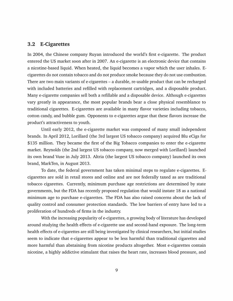
Figure 3 plots the trend in aggregate cigarette and e-cigarette sales over time for the
34,046 stores who are active in the panel each year between 2010-2012. E-cigarette sales were
low until mid 2011, when the quantity of units sold began to grow rapidly. The plot shows that
there is seasonality in the quantity of cigarette packs sold with lower sales during the winter
and higher sales during summer months.
13
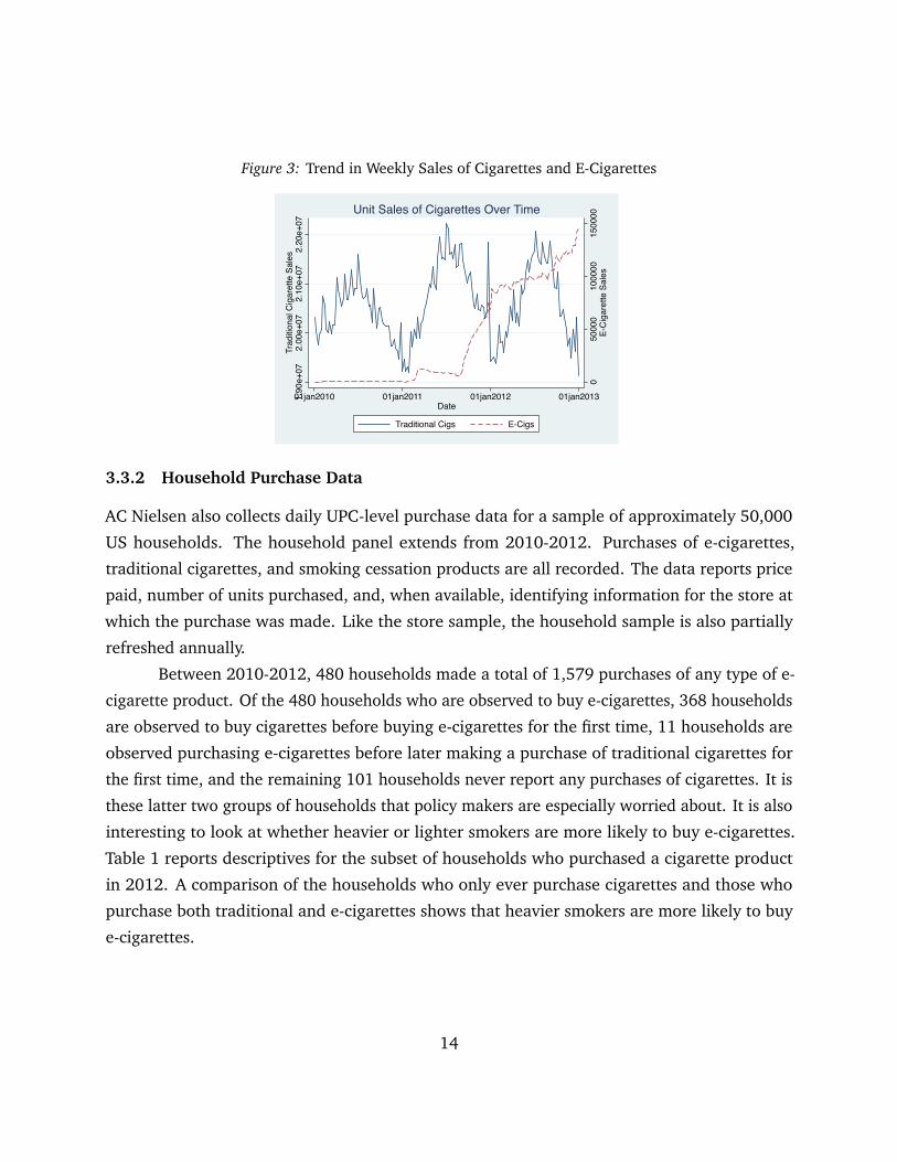
Figure 3: Trend in Weekly Sales of Cigarettes and E-Cigarettes
050
000
1000
0015
0000
E-Ci
gare
tte S
ales
1.90
e+07
2.00
e+07
2.10
e+07
2.20
e+07
Trad
itiona
l Cig
aret
te S
ales
01jan2010 01jan2011 01jan2012 01jan2013Date
Traditional Cigs E-Cigs
Unit Sales of Cigarettes Over Time
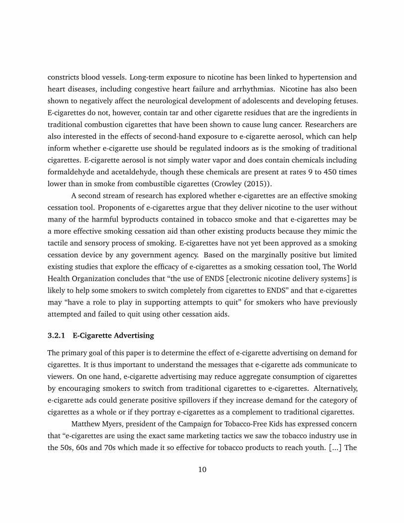
3.3.2 Household Purchase Data
AC Nielsen also collects daily UPC-level purchase data for a sample of approximately 50,000
US households. The household panel extends from 2010-2012. Purchases of e-cigarettes,
traditional cigarettes, and smoking cessation products are all recorded. The data reports price
paid, number of units purchased, and, when available, identifying information for the store at
which the purchase was made. Like the store sample, the household sample is also partially
refreshed annually.
Between 2010-2012, 480 households made a total of 1,579 purchases of any type of e-
cigarette product. Of the 480 households who are observed to buy e-cigarettes, 368 households
are observed to buy cigarettes before buying e-cigarettes for the first time, 11 households are
observed purchasing e-cigarettes before later making a purchase of traditional cigarettes for
the first time, and the remaining 101 households never report any purchases of cigarettes. It is
these latter two groups of households that policy makers are especially worried about. It is also
interesting to look at whether heavier or lighter smokers are more likely to buy e-cigarettes.
Table 1 reports descriptives for the subset of households who purchased a cigarette product
in 2012. A comparison of the households who only ever purchase cigarettes and those who
purchase both traditional and e-cigarettes shows that heavier smokers are more likely to buy
e-cigarettes.
14
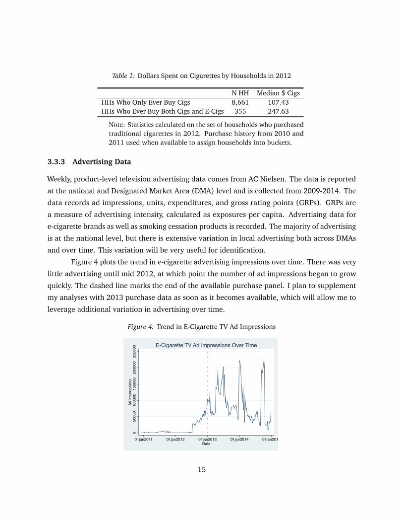
Table 1: Dollars Spent on Cigarettes by Households in 2012
N HH Median $ CigsHHs Who Only Ever Buy Cigs 8,661 107.43HHs Who Ever Buy Both Cigs and E-Cigs 355 247.63
Note: Statistics calculated on the set of households who purchasedtraditional cigarettes in 2012. Purchase history from 2010 and2011 used when available to assign households into buckets.
3.3.3 Advertising Data
Weekly, product-level television advertising data comes from AC Nielsen. The data is reported
at the national and Designated Market Area (DMA) level and is collected from 2009-2014. The
data records ad impressions, units, expenditures, and gross rating points (GRPs). GRPs are
a measure of advertising intensity, calculated as exposures per capita. Advertising data for
e-cigarette brands as well as smoking cessation products is recorded. The majority of advertising
is at the national level, but there is extensive variation in local advertising both across DMAs
and over time. This variation will be very useful for identification.
Figure 4 plots the trend in e-cigarette advertising impressions over time. There was very
little advertising until mid 2012, at which point the number of ad impressions began to grow
quickly. The dashed line marks the end of the available purchase panel. I plan to supplement
my analyses with 2013 purchase data as soon as it becomes available, which will allow me to
leverage additional variation in advertising over time.
Figure 4: Trend in E-Cigarette TV Ad Impressions
050
000
1000
0015
0000
2000
0025
0000
Ad Im
pres
sions
01jan2011 01jan2012 01jan2013 01jan2014 01jan2015Date
E-Cigarette TV Ad Impressions Over Time
15
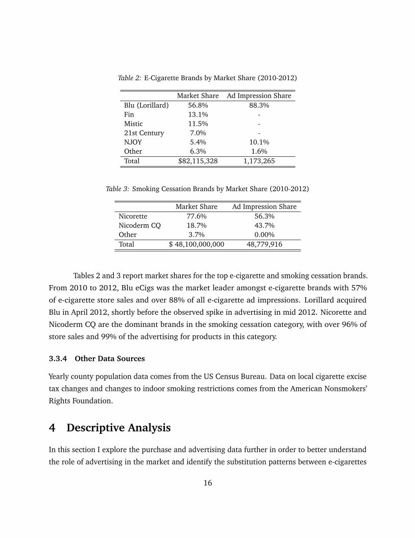
Table 2: E-Cigarette Brands by Market Share (2010-2012)
Market Share Ad Impression ShareBlu (Lorillard) 56.8% 88.3%Fin 13.1% -Mistic 11.5% -21st Century 7.0% -NJOY 5.4% 10.1%Other 6.3% 1.6%Total $82,115,328 1,173,265
Table 3: Smoking Cessation Brands by Market Share (2010-2012)
Market Share Ad Impression ShareNicorette 77.6% 56.3%Nicoderm CQ 18.7% 43.7%Other 3.7% 0.00%Total $ 48,100,000,000 48,779,916
Tables 2 and 3 report market shares for the top e-cigarette and smoking cessation brands.
From 2010 to 2012, Blu eCigs was the market leader amongst e-cigarette brands with 57%
of e-cigarette store sales and over 88% of all e-cigarette ad impressions. Lorillard acquired
Blu in April 2012, shortly before the observed spike in advertising in mid 2012. Nicorette and
Nicoderm CQ are the dominant brands in the smoking cessation category, with over 96% of
store sales and 99% of the advertising for products in this category.
3.3.4 Other Data Sources
Yearly county population data comes from the US Census Bureau. Data on local cigarette excise
tax changes and changes to indoor smoking restrictions comes from the American Nonsmokers’
Rights Foundation.
4 Descriptive Analysis
In this section I explore the purchase and advertising data further in order to better understand
the role of advertising in the market and identify the substitution patterns between e-cigarettes
16
and traditional cigarettes. First, using market-level data I show that e-cigarette advertising
increases demand for e-cigarettes and decreases demand for traditional cigarettes. Next, I
illustrate the substitution patterns between traditional and e-cigarettes and show evidence of
addiction using the household purchase data.
4.1 Identifying Advertising Effects with Aggregate Data
4.1.1 Identification Strategy
I am ultimately interested in measuring the causal effect of e-cigarette advertising on cigarette
demand. Identifying the causal effect of advertising is complicated by the fact that local
advertising is not assigned randomly. The concern is that firms are targeting higher levels of
advertising to markets with higher demand. If not accounted for, this endogeneity would lead
to biased estimates of the effects of e-cigarette advertising.
I address this endogeneity concern by exploiting a discontinuity in local advertising
markets that was first pointed out by Shapiro (2014). AC Nielsen delineates local television
markets or Designated Market Areas (DMAs) by grouping counties based on their predicted
interest in TV program content and quality of over-the-air TV signal. All households residing in
a given DMA will see the same television programming and ad content. Although nearly all
households now use cable or satellite dish as opposed to watching over-the-air, it is still the
case that television providers show households within a given DMA the same television content.
Thus, if advertisers don’t uniformly buy advertising across DMAs, households on opposite sides
of a DMA border can be exposed to different levels of advertising. I refer the reader to Shapiro
(2014) for a thorough discussion of television advertising markets.
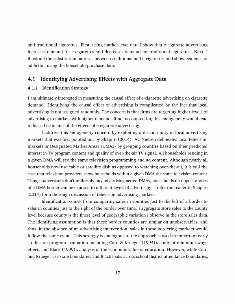
Identification comes from comparing sales in counties just to the left of a border to
sales in counties just to the right of the border over time. I aggregate store sales to the county
level because county is the finest level of geographic variation I observe in the store sales data.
The identifying assumption is that these border counties are similar on unobservables, and
thus, in the absence of an advertising intervention, sales in these bordering markets would
follow the same trend. This strategy is analogous to the approaches used in important early
studies on program evaluation including Card & Krueger (1994)’s study of minimum wage
effects and Black (1999)’s analysis of the economic value of education. However, while Card
and Krueger use state boundaries and Black looks across school district attendance boundaries,
17

Figure 5: Top 100 DMAs14:15 Saturday, May 23, 2015 114:15 Saturday, May 23, 2015 1
DMA boundaries do not necessarily coincide with state or other geo-political boundaries that
we worry would likely be correlated with advertising and demand for cigarettes. A map of the
top 100 DMAs ranked by viewership is shown in Figure 5.
DMAs tend to be centered around cities, while the borders between DMAs tend to fall in
more rural areas. Firms tend to set advertising for a given DMA based on the urban center of the
DMA, where the majority of the population resides. This suggests that we might see different
levels of advertising at the border between two DMAs, but that these differences are not being
driven by differences in the characteristics of households in these rural border areas. If sales in
bordering markets follow the same trend in the absence of an advertising intervention, we can
think of each border as an experiment with two treatment groups.
Take, for example, the border between the Louisville, KY and Lexington, KY DMAs shown
in Figure 6. There are 8 counties in the Louisville DMA that share a border with a county in the
Lexington DMA and 6 counties in the Lexington DMA that share a border with a county in the
Louisville DMA. The population of these border counties makes up a small share of the total
population of their corresponding DMAs; the border county population share of the Louisville
and Lexington DMAs are 9% and 12% respectively. I focus on borders between the top 100
DMAs, resulting in 151 borders and 302 border-markets. The mean and median border county
population shares across these border-markets are 9.4% and 16.7% respectively.
18
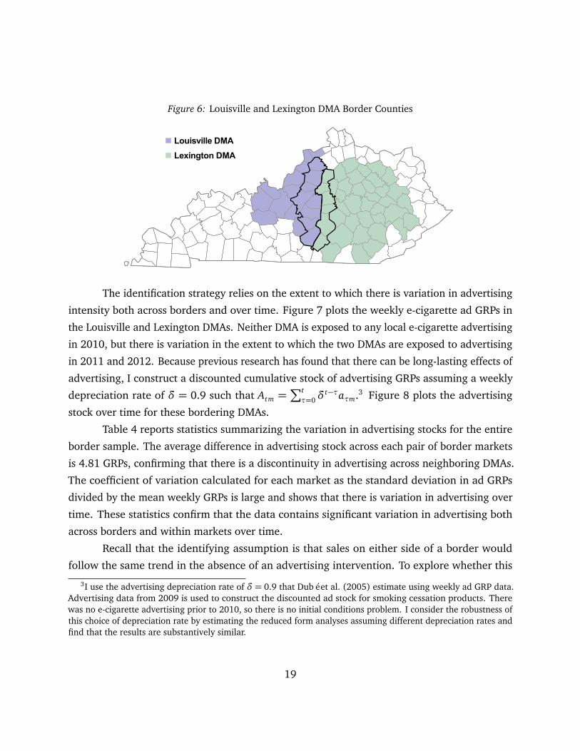
Figure 6: Louisville and Lexington DMA Border Counties
14:15 Saturday, May 23, 2015 114:15 Saturday, May 23, 2015 1
Louisville DMA
Lexington DMA
The identification strategy relies on the extent to which there is variation in advertising
intensity both across borders and over time. Figure 7 plots the weekly e-cigarette ad GRPs in
the Louisville and Lexington DMAs. Neither DMA is exposed to any local e-cigarette advertising
in 2010, but there is variation in the extent to which the two DMAs are exposed to advertising
in 2011 and 2012. Because previous research has found that there can be long-lasting effects of
advertising, I construct a discounted cumulative stock of advertising GRPs assuming a weekly
depreciation rate of δ = 0.9 such that Atm =∑tτ=0δ
t−τaτm.3 Figure 8 plots the advertising
stock over time for these bordering DMAs.
Table 4 reports statistics summarizing the variation in advertising stocks for the entire
border sample. The average difference in advertising stock across each pair of border markets
is 4.81 GRPs, confirming that there is a discontinuity in advertising across neighboring DMAs.
The coefficient of variation calculated for each market as the standard deviation in ad GRPs
divided by the mean weekly GRPs is large and shows that there is variation in advertising over
time. These statistics confirm that the data contains significant variation in advertising both
across borders and within markets over time.
Recall that the identifying assumption is that sales on either side of a border would
follow the same trend in the absence of an advertising intervention. To explore whether this
3I use the advertising depreciation rate of δ = 0.9 that Dubé et al. (2005) estimate using weekly ad GRP data.Advertising data from 2009 is used to construct the discounted ad stock for smoking cessation products. Therewas no e-cigarette advertising prior to 2010, so there is no initial conditions problem. I consider the robustness ofthis choice of depreciation rate by estimating the reduced form analyses assuming different depreciation rates andfind that the results are substantively similar.
19
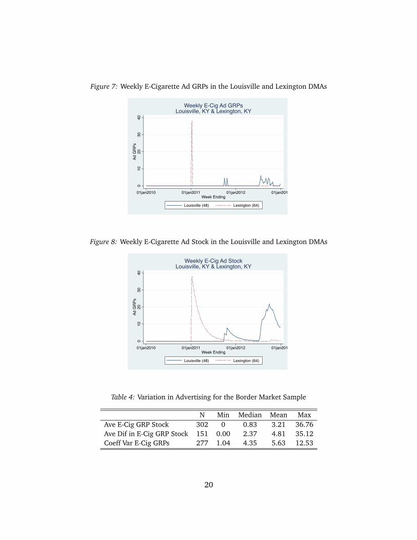
Figure 7: Weekly E-Cigarette Ad GRPs in the Louisville and Lexington DMAs
010
2030
40Ad
GR
Ps
01jan2010 01jan2011 01jan2012 01jan2013Week Ending
Louisville (48) Lexington (64)
Weekly E-Cig Ad GRPsLouisville, KY & Lexington, KY
Figure 8: Weekly E-Cigarette Ad Stock in the Louisville and Lexington DMAs
010
2030
40Ad
GR
Ps
01jan2010 01jan2011 01jan2012 01jan2013Week Ending
Louisville (48) Lexington (64)
Weekly E-Cig Ad StockLouisville, KY & Lexington, KY
Table 4: Variation in Advertising for the Border Market Sample
N Min Median Mean MaxAve E-Cig GRP Stock 302 0 0.83 3.21 36.76Ave Dif in E-Cig GRP Stock 151 0.00 2.37 4.81 35.12Coeff Var E-Cig GRPs 277 1.04 4.35 5.63 12.53
20
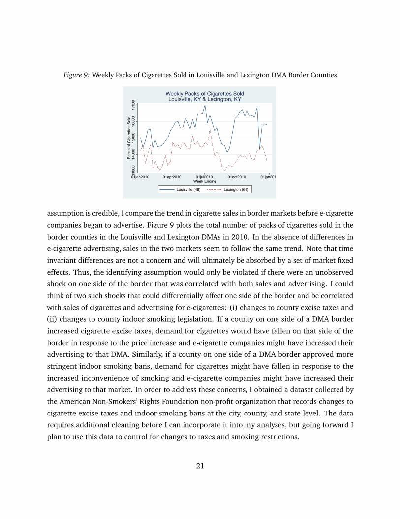
Figure 9: Weekly Packs of Cigarettes Sold in Louisville and Lexington DMA Border Counties
1300
014
000
1500
016
000
1700
0Pa
cks
of C
igar
ette
s So
ld
01jan2010 01apr2010 01jul2010 01oct2010 01jan2011Week Ending
Louisville (48) Lexington (64)
Weekly Packs of Cigarettes SoldLouisville, KY & Lexington, KY
assumption is credible, I compare the trend in cigarette sales in border markets before e-cigarette
companies began to advertise. Figure 9 plots the total number of packs of cigarettes sold in the
border counties in the Louisville and Lexington DMAs in 2010. In the absence of differences in
e-cigarette advertising, sales in the two markets seem to follow the same trend. Note that time
invariant differences are not a concern and will ultimately be absorbed by a set of market fixed
effects. Thus, the identifying assumption would only be violated if there were an unobserved
shock on one side of the border that was correlated with both sales and advertising. I could
think of two such shocks that could differentially affect one side of the border and be correlated
with sales of cigarettes and advertising for e-cigarettes: (i) changes to county excise taxes and
(ii) changes to county indoor smoking legislation. If a county on one side of a DMA border
increased cigarette excise taxes, demand for cigarettes would have fallen on that side of the
border in response to the price increase and e-cigarette companies might have increased their
advertising to that DMA. Similarly, if a county on one side of a DMA border approved more
stringent indoor smoking bans, demand for cigarettes might have fallen in response to the
increased inconvenience of smoking and e-cigarette companies might have increased their
advertising to that market. In order to address these concerns, I obtained a dataset collected by
the American Non-Smokers’ Rights Foundation non-profit organization that records changes to
cigarette excise taxes and indoor smoking bans at the city, county, and state level. The data
requires additional cleaning before I can incorporate it into my analyses, but going forward I
plan to use this data to control for changes to taxes and smoking restrictions.
21

Another impediment to the identification strategy could arise if cigarette companies
are strategically responding with their own marketing spending. According to the FTC, the
majority (85%) of marketing spending by cigarette companies in 2012 came in the form of price
discounts that were passed on to consumers. These discounts will be reflected in the prices in
my dataset and will thus be controlled for in the empirical analysis. The Nielsen advertising
database records print advertising expenditures for cigarette companies, but the vast majority
of this spending is at the national level. I expect its effects to be uniform on either side of DMA
borders and unlikely to be a problem for my identification strategy.
4.1.2 Fixed Effects Regression Results
In this section I discuss the implementation of the identification strategy and then present
the estimation results. At a high level, the approach is to only use data for border markets
and to include a rich set of market and border-time fixed effects that allow markets to have
different levels of sales and border-specific flexible time trends. I describe these steps below
in the context of the descriptive analysis. I later describe in Section 6 how to implement this
regression discontinuity approach within the context of my more complex non-linear model.
First, the sample is restricted to the set of stores who were active in the full panel from
2010-2012 and are located in a border county. All counties in a given DMA on a given border
are grouped together into a market. For example, the 8 counties in the Louisville DMA that
border the Lexington DMA form a market and sales in stores in these counties will be aggregated
to form total market sales. The 6 counties in the Lexington DMA that share a border with a
county in the Louisville DMA make up the comparison market. The dependent variables of
interest are total number of units of e-cigarettes sold, total number of packs of cigarettes sold,
and total number of nicotine patches sold by stores in each market each week. I focus on sales
of refill cartridges and disposable e-cigarettes because these products have similar prices and
are a better measure of e-cigarette consumption. To construct price series for each market from
the store sales data, I calculate the weighted average price for a pack of cigarettes and price of
a refill or disposable e-cigarette product. I construct the price series for the nicotine patch and
nicotine gum as the average price per unit paid for a patch and piece of gum.
I implement the identification strategy by including a set of market fixed effects and a
set of border-month fixed effects. The market fixed effects control for time invariant differences
across markets and allow each market to have its own average level of sales. Border-month
22

fixed effects allow each border to have its own flexible trend in sales that will, for example,
capture the observed seasonality in cigarette sales.
The differences in differences specification is shown in Equation 1. The unit of observation
is a market-border-week where m denotes market, b denotes border, and t denotes week. The
advertising stocks for e-cigarettes and smoking cessation products are denoted by Aemt and Aq
mt .
Equation 1 is estimated separately for e-cigarettes, cigarettes, and nicotine patches via OLS.
Standard errors are clustered at the market level. Table 5 presents the estimation results.
Qmt = βm + βbt +φeAemt +φqAq
mt +α~pmt + εmt (1)
First, looking at the first column in Table 5, there is a positive and significant effect of
e-cigarette advertising on e-cigarette sales. Advertising for the Nicorette and Nicoderm CQ
smoking cessation products generates positive spillovers that increase demand for e-cigarettes.
The own-price coefficient is negative and significant, while the cigarette and nicotine patch
cross-price coefficients are not statistically significant. The nicotine gum price coefficient is
estimated to be positive and statistically significant, suggesting that e-cigarettes and nicotine
gum are substitutes.
Columns 2 and 3 of Table 5 regress the number of packs of cigarettes sold in each market
on the set of independent regressors and fixed effects.4 The regression in column 2 does not
include e-cigarette price as a covariate while column 3 does. Thus, column 3 is estimated on a
smaller sample that only includes observations for the period after e-cigarettes entered each
market. In column 2 there is a negative and significant effect of e-cigarette advertising on
demand for traditional cigarettes. In column 3, the coefficient on e-cigarette advertising remains
negative but is no longer statistically significant after restricting to the sample with observed
e-cigarette prices. In both regressions the coefficient on smoking cessation advertising is not
statistically significant. I calculate own-price elasticities between -0.5 and -1.0 for traditional
cigarettes, which are similar to the range of cigarette price elasticities of -0.4 and -0.8 that have
been found in previous work (Gordon & Sun (2014)). The coefficient of e-cigarette price on
cigarette packs is not significant.
Finally, column 4 presents the results for the nicotine patch regression. The coefficient
on e-cigarette advertising is negative and highly statistically significant and the e-cigarette price
coefficient is positive and highly significant. These results are consistent with e-cigarettes and
4A carton counts as 10 packs.
23

Table 5: Difference in Differences Regression Results
(1) (2) (3) (4)Units E-Cigs Packs Cigs Packs Cigs Nicotine Patches
E-Cig Ad GRPs 0.240*** -27.719** -5.813 -0.281***(0.082) (11.600) (6.556) (0.088)
Smoking Cessation GRPs 0.017** 0.112 0.241 0.008(0.009) (0.481) (0.746) (0.010)
Price E-Cig -2.000*** - -8.438 2.242***(0.579) - (15.295) (0.533)
Price Pack Cigs -5.427 -2300.3*** -1020.3* 12.545(23.692) (545.1) (602.4) (14.079)
Price Nicotine Patch 0.801 -41.97 -17.17 -56.79***(1.053) (32.48) (46.20) (7.962)
Price Nicotine Gum 12.790** -499.7 -764.8** -212.8***(5.508) (491.5) (310.0) (37.60)
DMA-Border FE Y Y Y YMonth-Border FE Y Y Y YN Obs 21,960 44,920 22,923 22,923Own Price Elasticity -1.40 -0.97 -0.54 -5.44E-Cig Ad Elasticity 0.0076 -0.0014 -0.0004 -0.0026
Robust standard errors in parentheses*** p<0.01, ** p<0.05, * p<0.1
24

the nicotine patch being substitutes. The coefficient on the price of nicotine gum is negative,
suggesting that nicotine patches and gum may be complements. In their clinical practice
guidelines on treating tobacco use and dependence, the U.S. Department of Health and Human
Services (2008) reports that using nicotine gum and patches together leads to higher long-term
abstinence rates relative to other treatments. Surprisingly, in this specification the smoking
cessation advertising coefficient is not statistically significant.5
Together these results lead to the following conclusions. (1) E-cigarette advertising
increases demand for e-cigarettes and reduces demand for traditional cigarettes. (2) Consumers
treat e-cigarettes and smoking cessation products as substitutes. (3) Advertising for smoking
cessation products generates positive spillovers and increases demand for e-cigarettes. In the
next section, I further explore the substitution patterns between products using household
purchase panel data.
4.2 Substitution Patterns and Addiction in Household Data
Thus far, the aggregate data indicates that e-cigarette advertising increases demand for e-
cigarettes and reduces demand for traditional cigarettes. In this section, I examine household
panel data to determine whether households increase or decrease their consumption of cigarettes
after buying e-cigarettes, and whether there is evidence of cigarette addiction. Relative to the
aggregate data, the household data is more transparent in revealing these substitution patterns
over time.
To test for addiction, I analyze the weekly purchases of cigarettes for the 480 households
who ever buy an e-cigarette. Specifically, I analyze how recent cigarette purchases affect
whether the household purchases any cigarettes at all, denoted by the binary variable ci t , and
the number of packs of cigarettes the household purchases in that week, ci t . This test for
addiction is consistent with the Becker & Murphy (1988) model of addiction, in which past
consumption is complementary to current consumption. Because previous research has also
found evidence of stockpiling of cigarettes, a force that works in opposition to addiction, I
include three different variables related to past purchases to disentangle the effects of addiction
and stockpiling. First, I include ci t−1, a binary variable indicating whether the household
purchased any cigarettes last week. Then, I also separately include the quantity of cigarettes
5With ad stock depreciation rates smaller than δ = .6, the coefficient on smoking cessation advertising ispositive and significant.
25

purchased last week, ci t−1, and a stock variable that represents the total number of packs of
cigarettes purchased in the three weeks before that, Ci t . Separating the choice to purchase
last week from the quantity purchased last week, and the quantity of very recent purchases
(last week) from other recent purchases (the three preceding weeks) allows me to separate
addiction from stockpiling. I also include dummy variables indicating whether the individual
purchased an e-cigarette product in the preceding 4 weeks and whether they purchased a
smoking cessation product in the preceding 4 weeks, denoted by Ei t and Q i t respectively. Finally,
the regression includes household fixed effects, such that the coefficients are identified off of
within-household variation over time, and week fixed effects, which capture aggregate trends
and seasonality in cigarette sales. Standard errors are clustered at the household level.
ci t = αi +αt + β1 ci t−1 + β2ci t−1 + β3Ci t + γ1Ei t + γ2Q i t + εi t (2)
I use the same estimation equation when analyzing the number of packs of cigarettes households
purchase, ci t .
The first column of Table 6 presents the regression results when the binary choice to
purchase any cigarettes is the left hand side variable. The coefficient on purchasing cigarettes
in the previous week is positive and significant, which is consistent with addiction. However,
purchasing more packs in the previous week is less likely to be associated with a purchase
this week, which is consistent with stockpiling. More purchases over the previous 4 weeks,
which are less likely to have stock carry-over in the current week, are associated with a higher
purchase incidence this week, again consistent with addiction. These patterns provide evidence
that, setting stockpiling aside, households are more likely to buy in the current period if they
have purchased more in the past.
The second column presents the regression results when the number of cigarette packs
purchased is the left hand side variable. The coefficient on purchases in the previous week is
negative and significant, consistent with stockpiling. The coefficient on the e-cigarette dummy
variable is negative and significant, indicating that households reduce their purchase quantity
of cigarettes when they have recently purchased an e-cigarette product. The coefficient on
the smoking cessation dummy is also negative but is not statistically significant. Although we
cannot interpret these results as causal, the substitution patterns are consistent with e-cigarettes
and traditional cigarettes being substitutes.
In the preceding sections, I presented reduced form evidence that e-cigarette advertising
26

Table 6: Household Addiction and Substitution Patterns Between Cigarettes and E-Cigarettes
Cig Purchase Cig PacksIncidence Purchased
Cig Purchase in Previous Week 0.039*** 0.237(0.013) (0.342)
Cig Packs in Previous Week -0.002*** -0.165***(3.62e-04) (0.025)
Cig Packs in Previous 4 Weeks 6.42e-04** 0.020(2.48e-04) (0.018)
E-Cig in Previous 4 Weeks -0.006 -0.494***(0.007) (0.175)
Smoking Cessation in Previous 4 Weeks 0.004 -1.084(0.024) (0.949)
N Obs 23,040 23,040HH FE Y YWeek FE Y YMean DV 0.388 6.421Last Week Cig as % of DV 10.03% -Post E-Cig as % of DV - -7.70%
Robust standard errors in parentheses*** p<0.01, ** p<0.05, * p<0.1
27

increases demand for e-cigarettes and reduces demand for cigarettes. Analysis of household
panel data further showed that households tend to reduce their consumption of cigarettes after
they purchase e-cigarettes and that addiction is an important force at play in this market. In
the following section, I present a structural model of demand for cigarettes that is motivated by
these empirical findings. The model will allow me to (i) simultaneously account for advertising
effects and addiction, (ii) implement more efficient joint estimation using both aggregate and
household data, (iii) control for unobserved heterogeneity in preferences, and (iv) evaluate
counterfactual scenarios that predict the response in cigarette demand to a proposed ban of
e-cigarette TV advertising.
5 An Integrated Micro-Macro Model of Demand
5.1 Overview
My descriptive analysis of market-level sales and advertising data indicates that e-cigarette
advertising reduces demand for traditional cigarettes. These results suggest that banning
e-cigarette advertising may have unintended consequences and actually lead to an increase
in aggregate cigarette consumption. The magnitude of this effect is of great importance to
policy makers as they consider whether to impose a ban on advertising for e-cigarettes. In the
following sections, I develop a structural model of demand for cigarettes and use the estimated
preference parameters to predict the counterfactual demand for cigarettes that would have
been observed in the absence of e-cigarette advertising.
I specify a structural model that (i) harnesses the information content of both individual
and aggregate data in an efficient and internally consistent way, (ii) incorporates dynamic
dependences that arise as a result of nicotine addiction, and (iii) identifies advertising effects
accounting for endogeneity using the border strategy approach. The existing literature has
addressed each of these individually, but I believe my paper is the first to unify these objectives
within a single cohesive framework. I discuss each of these aspects of the model in turn below.
In theory, I could use either the aggregate or household-level data to estimate demand
for cigarettes. However, each dataset has its relative merits and limitations. The aggregate data
measures advertising effects with less noise and can be used to recover unobserved aggregate
demand shocks, while the household data is more transparent in revealing patterns of addiction
and heterogeneity in the population. For these reasons, I leverage both datasets to estimate
28
demand for cigarettes. Specifically, I propose an individual-level demand model that aggregates
in an internally consistent way, such that the equations that govern household and aggregate
demand are functions of the same parameters. In order to estimate the model, I adapt an
integrated estimation procedure developed by Chintagunta & Dubé (2005), who illustrate how
to combine household and aggregate store level data to estimate the parameters of a discrete
choice random coefficients model of demand. The intuition behind their estimation approach
is to take advantage of the relative merits of each dataset to simultaneously (i) estimate the
mean effects of marketing activities, (ii) account for endogeneity in prices, and (iii) allow for
heterogeneity across households. As Chintagunta and Dubé point out, although heterogeneity
in the population can be identified using only aggregate data (Berry et al. (1995)), household
panel data is more informative about heterogeneity than store level data. At the same time,
there is usually little to no information in household panel data that can be used to account for
the endogeneity of prices, but aggregate data can be used to account for the endogeneity of
prices (Berry et al. (1995)).6 Motivated by these facts, Chintagunta and Dubé propose a method
to use aggregate data to estimate mean preference parameters and address the endogeneity
problem and household-level data to estimate the distribution of heterogeneity.
I extend this micro-macro demand model to account for dynamic dependencies that
arise as a result of nicotine addiction. State-dependence is not incorporated in the Chintagunta
and Dubé approach, but it is key to the analysis of addiction. The incorporation of state
dependence, however, complicates the aggregate demand system considerably, since demand is
no longer independent across time. In order to capture this persistence across time, I adapt a
formulation due to Caves (2004). Caves presents an aggregate structural model of demand
for cigarettes that incorporates addiction as a form of category-level state dependence where a
consumer’s utility from buying a cigarette product in the current period is higher if he purchased
a cigarette product in the previous period. He allows for heterogeneity in the form of discrete
types, estimating his model with high and low types in ad responsiveness.7 I combine Caves’
model, which was developed originally for only aggregate data, with Chintagunta and Dubé’s
estimation strategy, while extending Caves’ algorithm significantly to allow for a continuous
distribution of heterogeneous preferences in price and ad responsiveness. I find that allowing for
6Subsequent work has shown that supplementing the model with household moments can generate morerealistic model-predicted substitution patterns (Petrin (2002) and Berry et al. (2004)).
7In another category, Horsky et al. (2012) also estimates an aggregate structural model with state dependence,though the model does not allow for unobserved heterogeneity.
29

a rich continuous distribution of heterogeneity is important to correctly separate the impact of
addiction – a form of state dependence – from persistent unobserved tastes, an observation well
known to econometricians at least since Heckman (1981). The incorporation of a continuous
distribution of heterogeneity increases the computational cost of the estimator significantly.
The final modeling challenge I face is how to incorporate the identification of advertising
effects within the structural model, an element that has not always been a focus of the existing
literature on nicotine addiction. The same intuition behind identification in the reduced form
setting holds in the structural model as well. I estimate the model only using data for stores
and individuals located within border markets, and I include market-border and border-time
fixed effects. In Section 6 I explain in further detail how the structural model accommodates
these fixed effects.
Ultimately, I contribute to the literature by combining these separate streams of research
to carefully identify advertising effects in a model with addiction using both individual and
aggregate data within a unified framework. While in theory Caves’ model is identified using
only aggregate data, in this paper I show how to incorporate individual level data to improve
the efficiency of estimation and the flexibility of the heterogeneity specification. I extend the
estimation procedure developed by Chintagunta & Dubé to a model with state dependence, and
I illustrate how regression discontinuity identification can be ported into the structural model.
In the sections below, I first lay out the equations characterizing individual-level demand
and then show how the model aggregates and accommodates unobserved heterogeneity. Next,
I describe the estimation procedure in more detail. Finally, I present the estimation results
and use the model estimates to consider the implications of a proposed ban on e-cigarette
advertising.8
5.2 Individual Level Model
I specify an individual-level discrete choice model where consumers choose whether to buy a
pack of cigarettes, a carton of cigarettes, or not to make a purchase. To incorporate addiction,
an important characteristic of the cigarette market, I allow utility from consuming in the current
period to be increasing in consumption in the previous period. This simple model of addiction
is consistent with the Becker & Murphy (1988) model of addiction in which past consumption
8In Appendix A I use model simulations to show that the model is well identified and that combining aggregateand household data leads to increased estimation efficiency.
30

is complementary to current consumption.
Denote an individual’s indirect utility function from consuming product j by equation 3.
The indirect utility is a function of observed variables and unobserved product characteristics.
Observed variables include current prices p and e-cigarette and smoking-cessation advertising~A. These variables, together with a set of product intercepts, are grouped into the matrix X .
Also observed is an indicator ci t−1 denoting whether the individual consumed any of the inside
goods in the previous period. Note that addiction operates at the category level and ci t−1 is not
product specific; ci t−1 takes on a value of 1 if the individual purchased either a pack or a carton
of cigarettes in the previous period and a 0 otherwise. The unobserved (to the econometrician)
components of the indirect utility function include ξ jmt which captures systematic shocks to
aggregate demand including, for example, unobserved marketing activity, and εi j t , a stochastic
error term which is assumed to be distributed type I extreme value. The deterministic part of
utility from consuming the outside good is normalized to 0.
ui j t = β j +αp j t +φ~Amt + γci t−1 + ξ jmt + εi j t (3)
ui0t = εi0t (4)
Integrating out the distribution of stochastic errors εi j t , the probability that an individual
will purchase product j is given by equation 5.
Pi j t(X i t , ci t−1) =eX j tθ+ξ j t+γci t−1
1+∑
k eXktθ+ξkt+γci t−1(5)
5.3 Aggregate Model
Conditional on past consumption status, the probability of buying a product is just the logit
probability given by equation 5. Let s jmt denote the market share of product j in market m in
week t and s0mt denote the market share of the outside good. I calculate aggregate market shares
by weighting the purchase probabilities conditional on consumption status by the probability of
having that consumption status, which in this case is just the combined market shares of the
inside goods in the previous period.
s jmt = Pr( j|X jmt , ct−1 = 1)Pr(ct−1 = 1) + Pr( j|X jmt , ct−1 = 0)Pr(ct−1 = 0) (6)
=eX jmtθ+ξ jmt+γ
1+∑
k eXkmtθ+ξkmt+γ(1− s0mt−1) +
eX jmtθ+ξ jmt
1+∑
k eXkmtθ+ξkmts0mt−1 (7)
31
5.4 Incorporating Unobserved Heterogeneity
Thus far, I have shown how to derive aggregate demand from a homogenous demand model
with state dependence. In this section I extend the model to include unobserved heterogeneity
in consumer types. The key insight is that the joint distribution of heterogeneity and state
dependence is not stationary; rather, it evolves over time. For example, if consumers vary in their
sensitivity to price, then an increase in price will decrease the probability that price-sensitive
consumers buy today, which affects the joint distribution of consumer types and consumption
states in the next period. In particular, prices in the current period affect the joint distribution
of state dependence and heterogeneity in all subsequent periods. I allow the coefficients on
price and advertising to vary across the population, as shown in equation 8.
ui j t = β j +αi p j t +φi~Amt + γci t−1 + ξ jmt + εi j t (8)
As in the previous section, in order to obtain aggregate market shares I integrate out
unobserved heterogeneity and the stochastic demand shocks. In the model with heterogeneity,
I calculate aggregate market shares by integrating the purchase probabilities conditional on
consumption status and consumer type against the joint distribution of consumption status and
consumer heterogeneity.
s j t =
∫
Θ×0,1Pr( j|θi, ct−1)dFθi×c (9)
The discussion above does not assume any particular joint distribution between unobserved het-
erogeneity and state dependence. In the estimation section below, I make specific assumptions
about that distribution and show how to numerically evaluate the above integral.
Discussion
Before moving on to the estimation procedure, I first discuss some of my modeling assumptions.
First is the decision to use a discrete choice model instead of explicitly modeling purchase
quantities. Past work on addiction has assumed that addiction operates through the effect of
past purchase quantities on current purchase quantity (Becker & Murphy (1988), Gordon & Sun
(2014)). The household panel data would in theory allow me to model quantities; however, the
panel is thin. The aggregate data is richer and allows me to identify advertising effects with
32

more precision, but it limits my ability to model purchase quantities.9 In order to be able to
harness the richness of the aggregate data, I choose to model purchase incidence in a discrete
choice framework. Within this framework, I am able to accommodate purchase quantities by
allowing consumers to make a discrete choice over pack sizes. Cigarettes are primarily sold in
uniform packages of packs (20 cigarettes) and cartons (10 packs), so the pack size proliferation
that is often observed in CPG categories is not binding in this case.
A separate but related assumption is that only the previous week’s purchase decision
affects current period consumption and that consumers are not forward looking. An assumption
closer to observed consumer behavior and patterns of addiction might allow additional lags of
purchase decisions to affect current choices. I choose to work with the simpler one period lag
because the model with state dependence can be estimated using aggregate data. Although this
may be a strong restriction on consumer behavior, my econometric specification is still flexible.
My estimation allows for heterogeneity across households and includes market and time fixed
effects, which allow me to capture a variety of observed data patterns.
6 Estimation and Results
6.1 Estimation with Unobserved Heterogeneity
The model discussion above did not rely on any specific assumptions about the distribution
of unobserved heterogeneity. In my model implementation, I assume that unobserved hetero-
geneity follows a normal distribution, but to facilitate exposition, I first introduce the model
with R discrete types. Specifically, suppose individuals are drawn from a distribution with R
latent types such that an individual’s preference parameter vector is θr ∈ Θ. For each type, the
probability of purchasing product j is again the familiar logit probability Pr( j|θr , ct−1 = 1) if
the individual purchased in the previous period and Pr( j|θr , ct−1 = 0) if they did not.
In the initial period, the population of consumers is distributed across these types
and consumption states according to some joint distribution Pr(θr , ct=0).10 In subsequent
periods, the marginal probability of being a certain type Pr(θr) remains constant, but the joint
9Hendel & Nevo (2013) model purchase quantities using aggregate data, but need to impose other simplifyingassumptions in order to make their model tractable with aggregate data.
10Equation 10 relies on an initial condition prc = Pr(θr , ct=0) that pins down the initial joint distribution. Idiscuss how I resolve this initial conditions problem in more detail in the estimation section below.
33

distribution of consumer types and consumption status Pr(θr , ct) evolves as the heterogeneous
population responds to variation in prices and advertising. The joint distribution updates each
period according to the recursion in equation 10.
Pr(θr , ct = 1) = Pr(ct = 1|θr , ct−1 = 1)× Pr(θr , ct−1 = 1)
+ Pr(ct = 1|θr , ct−1 = 0)× Pr(θr , ct−1 = 0)(10)
The recursion shows that the probability of being a specific type r and smoking in the current
period ct = 1 is equal to the probability that a smoker of type r continues smoking in the current
period plus the probability that a non-smoker of type r begins smoking in the current period.
Finally, aggregate market shares are obtained in the model with R latent types by
weighting the logit probability of purchase for each individual type by the joint distribution of
types and consumption status in the population. Specifically, the integral describing market
shares in equation 9 becomes a summation over discrete types, as shown in equation 11.
s j t =R∑
r=1
[Pr( j|θr , ct−1 = 1)× Pr(θr , ct−1 = 1) + Pr( j|θr , ct−1 = 0)× Pr(θr , ct−1 = 0)] (11)
Now, I discuss how to extend the model to allow for a continuous heterogeneity dis-
tribution. I assume that the distribution of random coefficients follows a normal distribution,
and I estimate the mean θ and variance Σ of the distribution. Let νi ∼ N(0,1) and Λ be the
Cholesky decomposition of Σ s.t. θi = θ + Λνi ∼ N(θ ,Σ). The indirect utility function in
equation 8 can be decomposed into common and individual-specific components, as shown
in equation 12, where δ jmt = X jmt θ + ξ jmt captures the mean aggregate utility level and
µi j t(X jmt , ci t−1;Σ,γ) = X jmtΛνi + γci t−1 represents heteroskedastic deviations from the mean
utility level. Note that δ is the mean utility level for those who did not consume in the previous
period, and addiction, or the increase in utility coming from having consumed in the previous
period, is captured in µ.
ui j t = β j +αi p j t +φi~Amt + γci t−1 + ξ jmt + εi j t
= δ jmt(X jmt ,ξ jmt; θ ) +µi j t(X jmt , ci t−1;Σ,γ) + εi j t
(12)
The additional layer of complication in incorporating a continuous distribution of unobserved
heterogeneity is in how to evaluate the integral in equation 9 and how to update the joint
distribution of unobserved heterogeneity and state dependence each period. In a standard
random coefficients model, the typical approach to integrating out unobserved heterogeneity
34

is to take draws from the latent distribution and approximate the integral using Monte Carlo
integration. The key insight to implementation of a continuous distribution of unobserved
heterogeneity in the aggregate model with state dependence is that once R draws are taken
from the latent normal, we are basically back in the world of an R-type latent class model.
Equation 10 approximates the joint distribution of heterogeneity and state dependence and
equation 11 can be used to obtain the model-predicted aggregate market shares.
6.2 Estimation Procedure
At a high level, I estimate the mean utility parameters θ and recover unobserved demand
shocks ξ jmt from aggregate data and estimate the heterogeneity distribution Σ and addiction
parameter γ from household panel data. The estimation steps are described in detail below.
1. Aggregate Data Step: Given a guess of the heterogeneity and addiction parameters (Σ, γ),for each market m, product j, and time period t, I compute δ jmt = X jmt θ + ξ jmt that
equates the model predicted market share to the observed market share in the aggregate
data. I calculate observed market shares by dividing total store sales in each market by
the adult population of that market. The model-predicted market share s(X ,δ;Σ,γ) is
given by equation 9. In practice, I approximate the integral over the joint distribution
of consumer heterogeneity and state dependence using Monte Carlo integration. I take
R draws νr ∼ N(0,1) and for the given guess of Σ calculate θr = θ + Λνr ∼ N(θ , Σ).Then I use equations 10 and 11 to calculate the model-predicted aggregate market shares.
Conditional on Σ and γ, the model predicted share is given by
s jmt =R∑
r=1
eδ jmt+X jmt Λνr+γ
1+∑
k eδkmt+Xkmt Λνr+γ× Pr(θr , ct−1 = 1)
+eδ jmt+X jmt Λνr
1+∑
k eδkmt+Xkmt Λνr× Pr(θr , ct−1 = 0)
(13)
and the joint distribution of heterogeneity and state dependence is given by
Pr(θr , ct = 1) =
∑
k eδkmt+Xkmt Λνr+γ
1+∑
k eδkmt+Xkmt Λνr+γ× Pr(θr , ct−1 = 1)
+
∑
k eδkmt+Xkmt Λνr
1+∑
k eδkmt+Xkmt Λνr× Pr(θr , ct−1 = 0)
(14)
35

The recursion in equation 14 relies on knowing the joint distribution of heterogeneity and
consumption status, pr1 = Pr(θr , ct=0 = 1) and pr0 = Pr(θr , ct=0 = 0), in the initial period.
The literature has typically resolved this type of initial conditions problem by either treating
the initial probability distribution as parameters of the model to estimate, or by using an
initial period of data as a burn-in period to forward simulate the distribution (Erdem et al.
(2003)). I take the second approach and use the first quarter of data for each market to
forward simulate the joint distribution. For each guess of the parameters, I re-calculate
the series of probabilities governing the evolving joint distribution of heterogeneity and
state dependence for the initial burn-in period and obtain pr1 and pr0.11 I then use the
remaining data for each market, starting in the second available quarter, as the initial
period in estimation.
With the equations describing model-predicted shares in hand, I calculate the δs that
equate observed and model-predicted shares using the BLP contraction mapping algorithm
described in equation 15 (Berry et al. (1995)). The values of δ jmt must be calculated
iteratively each period because state dependence causes the current period share to
depend on the previous unobserved demand shock ξ jmt−1.
δh+1m·t = δ
hm·t + ln Sm·t − ln s(Xm·t ,δ
hm·t; Σ, γ) (15)
2. Household Data Step: Given the current guess of δ, I estimate Σ and γ via maximum
likelihood with household data. Each household is matched to its aggregate data counter-
part. Substituting the appropriate δ into the household’s indirect utility function,12 the
probability that a household buys a given product in a given period is given by equation
11I assume equal probabilities of smoking and not smoking for each type in the first week of the burn-in period,such that the probability of having a given type and smoking consumption status at the beginning of the burn-inperiod is equal to 1
2R . I have tried a variety of different starting values and found that the joint distribution convergesto the same steady state within the burn-in period.
12In model simulations in Appendix A, I assume that households face the same prices as those used to generatethe aggregate data. Then the δ that equates the model-predicted aggregate market shares to the observed marketshares can just be plugged into the household ML model. In the actual dataset used for estimation, the householdprice series records the prices actually paid by households while the aggregate price series records the average priceof cigarettes in that market, which will not be the same. In order to resolve this inconsistency, on each iteration Icalculate a household-specific δi . For each iteration or guess of θ2, I use the BLP contraction to solve for δm. Ithen estimate θOLS
1 = (β , α, φ) and back out ξm = δm − X1θ1 which is used to construct the household-specificδim = βm + αpi + φAm + ξm using the household price series pi . These household-specific δi ’s are then pluggedinto the likelihood function for the household ML estimation.
36

16. Integrating out the distribution of unobserved heterogeneity, the likelihood for each
individual is then given by equation 17. In practice, I approximate the integral using a
Monte Carlo simulation using the same R draws from the standard normal, and I esti-
mate the parameters Σ and γ by maximizing the likelihood in equation 18 via maximum
simulated likelihood.
Pi j t(X imt , δimt , ci t−1,Σ,γ) =exp[δim jt + X im jtΛνi + γci t−1]
1+∑K
k=1 exp[δimkt + X imktΛνi + γci t−1](16)
Li(Yi|X i, δi;Σ,γ) =
∫ Ti∏
t=1
J∏
j=1
Pi j t(X i, δi, ci t−1,Σ,γ)Yi j t dFν (17)
L (Y |X , δ;Σ,γ) =N∑
i=1
log[Li(Yi|X i, δi;Σ,γ)] (18)
3. Iterate Until Convergence: I iterate steps 1 and 2 until the estimated parameters (δ,Σ,γ)do not differ by more than a threshold of 10−6.
4. Estimate Linear Parameters from Aggregate Data: After the model parameters have
converged, I then use the fact that δmjt = Xmjt θ + ξmjt to estimate the linear parameters
θ . For now, I estimate ˆθ = (X ′X )−1X ′δ via OLS. In future work I hope to account for the
potential endogeneity of prices by instrumenting for price in a linear IV regression.
I calculate standard errors for Σ and γ, the model parameters identified off of the
household data, by inverting the hessian at the optimum of the likelihood function. Standard
errors for the remaining linear parameters are calculated using a parametric bootstrap. I take
draws from the asymptotic distribution of Ω = (Σ,γ), and for each draw ωn I calculate the
implied vector δ(ωn) that equates observed and model-predicted shares. Then for each δ(ωn)vector, I estimate the linear parameters θn. The standard errors are inferred from the variance
of the distribution of the estimates of the linear parameters.
37

6.3 Identification
Before presenting the model estimates, I first discuss identification and highlight how I incorpo-
rate the border counties identification strategy into the estimation of the structural model. I
estimate the model using aggregated store data for only those stores in border county markets
and household data for only those households who reside within border counties. Thus, the
same regression discontinuity identification from the linear model applies here — the nonlinear
estimator is also only based on the behavior of marginal consumers at borders. In total I have
data for 272 markets and 150 households. The fact that the linear parameters are estimated
in a simple linear regression allows me to continue to include border-market and border-time
fixed effects. Specifically, I include a set of 1,587 border-market and border-quarter fixed effects
in the structural estimation. It would be impossible to include this many parameters in a typical
non-linear optimization routine. The linear regression stage is thus an important component
of the model that allows me to incorporate regression discontinuity identification into the
structural model.
Finally, the household purchase data identifies the parameters pinning down the hetero-
geneity distribution and state dependence, while the aggregate data identifies the mean utility
parameters. Although state dependence can be identified using aggregate data based on the
co-movement of current market shares and variation in past prices, household data allows us
to explicitly observe the dependence across a given household’s purchases over time. Similar
intuition applies regarding the identification of unobserved heterogeneity.
6.4 Estimation Results
Table 7 presents the estimated model parameters. The first column reports estimates for
the homogeneous model. The second column reports estimates for the model with random
coefficients on price and advertising. Focusing on the estimates for the model with heterogeneity,
the mean coefficients on price and advertising for e-cigarettes and smoking cessation products
are all estimated to be negative. The estimated standard deviations of the heterogeneity
distribution are large relative to the means, especially for e-cigarette advertising, implying that
advertising will increase demand for cigarettes for some individuals. The difference in product
intercepts βp − βc gives the estimated relative preference for packs over cartons of cigarettes.
Once heterogeneity is included in the model, the magnitude of the addiction parameter γ
38

decreases. In the absence of heterogeneity, any serial correlation generated by unobserved
heterogeneity is absorbed into γ. This result is consistent with the findings of Dubé et al. (2010).
Table 7: Model Estimation Results
Homogeneous Heterogeneousθ σθ
α -0.7920 -0.6701 0.5678(0.0099) (0.0246) (0.0077)
φe 0.0003 -0.0242 0.0255(0.0002) (0.0005) (0.0009)
φq 0.0002 -0.1866 0.1199(0.0002) (0.0004) (0.0005)
βp − βc 3.5708 3.6025(0.0045) (0.0115)
γ 3.2576 0.5409(0.0345) (0.0530)
Market FEs Y YBorder-Quarter FEs Y Y
In order to build intuition around the estimation results, I calculate the implied short-
and long-run demand elasticities for each market. The short run elasticity captures the re-
sponsiveness of demand to a one-time price increase in the same week. I calculate short-run
elasticities using equation 19. The distribution across markets of the average short-run demand
elasticity of a pack of cigarettes is shown in Figure 10. The mean short-run demand elasticity
across markets is -0.75.
η jmt =p jmt
s jmt
∂ s jmt
∂ p jmt
=p jmt
s jmt
∫
Θ×0,1αisi jmt|c(1− si jmt|c)dFi×c
=p jmt
s jmt
∑
(θr×ct−1)∈θ1,...,θR×0,1
αrsr jmt|ct−1(1− si jmt|ct−1
)Pr(θr , ct−1)
(19)
Since the effect of addiction creates dynamic dependencies in demand over time, I also
plan to look at the long run elasticity of demand to see how a price increase in one week affects
demand in future periods. The long-run elasticity requires forward simulating demand.
39
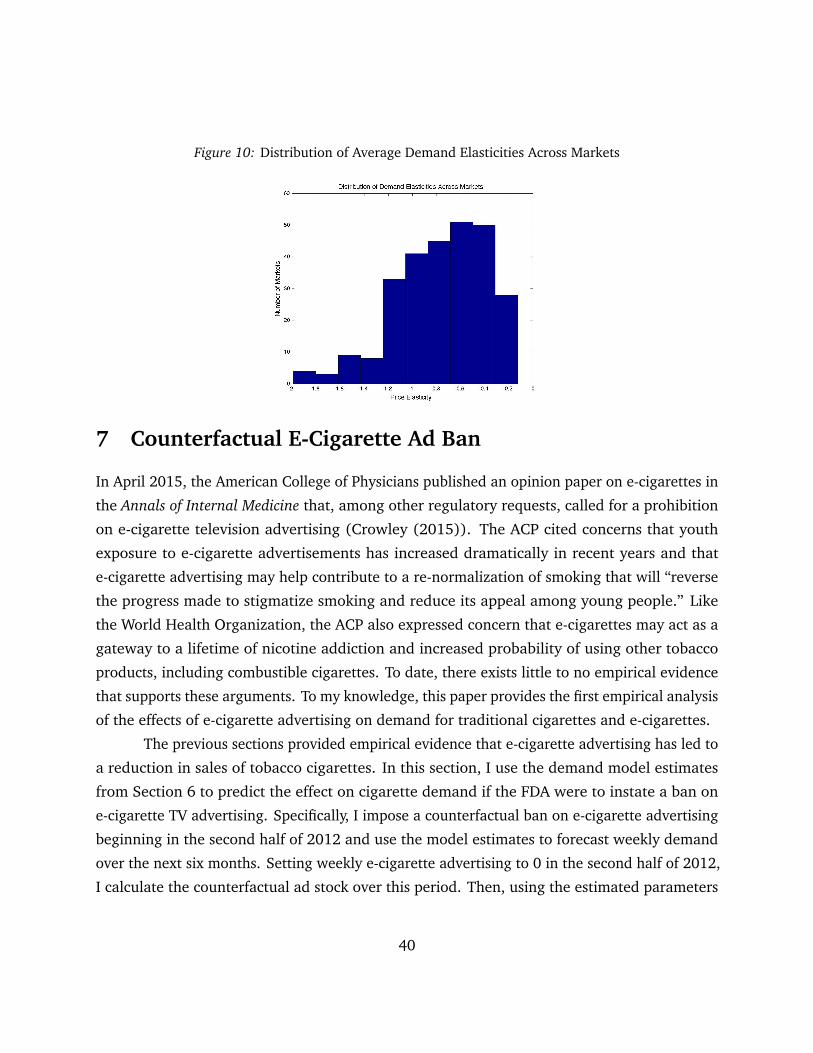
Figure 10: Distribution of Average Demand Elasticities Across Markets
7 Counterfactual E-Cigarette Ad Ban
In April 2015, the American College of Physicians published an opinion paper on e-cigarettes in
the Annals of Internal Medicine that, among other regulatory requests, called for a prohibition
on e-cigarette television advertising (Crowley (2015)). The ACP cited concerns that youth
exposure to e-cigarette advertisements has increased dramatically in recent years and that
e-cigarette advertising may help contribute to a re-normalization of smoking that will “reverse
the progress made to stigmatize smoking and reduce its appeal among young people.” Like
the World Health Organization, the ACP also expressed concern that e-cigarettes may act as a
gateway to a lifetime of nicotine addiction and increased probability of using other tobacco
products, including combustible cigarettes. To date, there exists little to no empirical evidence
that supports these arguments. To my knowledge, this paper provides the first empirical analysis
of the effects of e-cigarette advertising on demand for traditional cigarettes and e-cigarettes.
The previous sections provided empirical evidence that e-cigarette advertising has led to
a reduction in sales of tobacco cigarettes. In this section, I use the demand model estimates
from Section 6 to predict the effect on cigarette demand if the FDA were to instate a ban on
e-cigarette TV advertising. Specifically, I impose a counterfactual ban on e-cigarette advertising
beginning in the second half of 2012 and use the model estimates to forecast weekly demand
over the next six months. Setting weekly e-cigarette advertising to 0 in the second half of 2012,
I calculate the counterfactual ad stock over this period. Then, using the estimated parameters
40
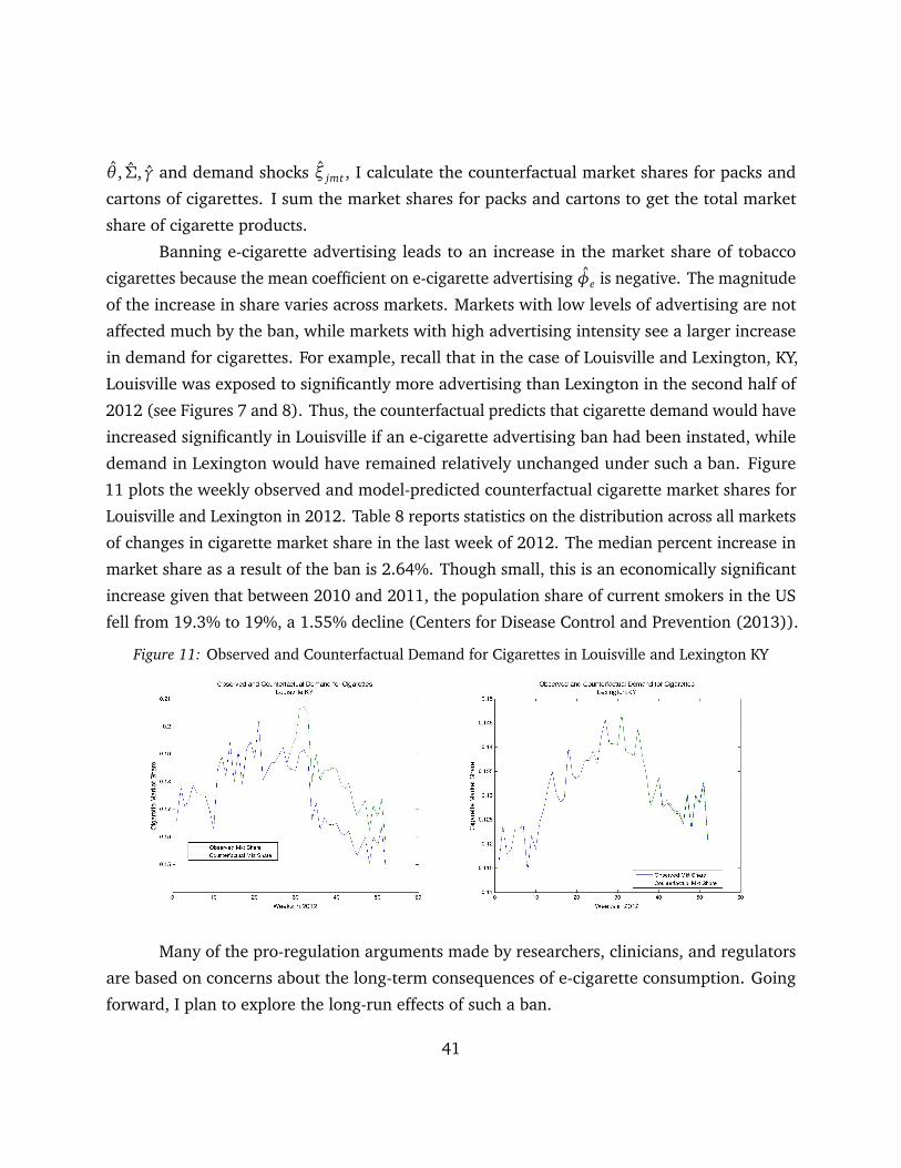
θ , Σ, γ and demand shocks ξ jmt , I calculate the counterfactual market shares for packs and
cartons of cigarettes. I sum the market shares for packs and cartons to get the total market
share of cigarette products.
Banning e-cigarette advertising leads to an increase in the market share of tobacco
cigarettes because the mean coefficient on e-cigarette advertising φe is negative. The magnitude
of the increase in share varies across markets. Markets with low levels of advertising are not
affected much by the ban, while markets with high advertising intensity see a larger increase
in demand for cigarettes. For example, recall that in the case of Louisville and Lexington, KY,
Louisville was exposed to significantly more advertising than Lexington in the second half of
2012 (see Figures 7 and 8). Thus, the counterfactual predicts that cigarette demand would have
increased significantly in Louisville if an e-cigarette advertising ban had been instated, while
demand in Lexington would have remained relatively unchanged under such a ban. Figure
11 plots the weekly observed and model-predicted counterfactual cigarette market shares for
Louisville and Lexington in 2012. Table 8 reports statistics on the distribution across all markets
of changes in cigarette market share in the last week of 2012. The median percent increase in
market share as a result of the ban is 2.64%. Though small, this is an economically significant
increase given that between 2010 and 2011, the population share of current smokers in the US
fell from 19.3% to 19%, a 1.55% decline (Centers for Disease Control and Prevention (2013)).
Figure 11: Observed and Counterfactual Demand for Cigarettes in Louisville and Lexington KY
Many of the pro-regulation arguments made by researchers, clinicians, and regulators
are based on concerns about the long-term consequences of e-cigarette consumption. Going
forward, I plan to explore the long-run effects of such a ban.
41

Table 8: Counterfactual Increase in Cigarette Demand Across Markets
Min 25% Median 75% MaxIncrease in Mkt Share 0.00 0.00 0.10 0.49 7.50Pct Increase in Mkt Share 0.00% 0.29% 2.64% 12.06% 151.49%
8 Conclusions and Future Work
To my knowledge, this paper is the first to empirically analyze the effects of e-cigarette ad-
vertising on demand for traditional cigarettes and e-cigarettes. Using both descriptive and
structural methods, I show that e-cigarette advertising decreases demand for cigarettes. My
research contributes to the ongoing policy debate as to whether e-cigarette TV advertising
should be banned and suggests that a ban on e-cigarette advertising may have unintended
consequences. More generally, my approach contributes to the study of advertising in categories
with state dependence and to the analysis of substitution and complementarities in demand
across categories.
Although this paper takes an important first step towards better understanding the role
of e-cigarette advertising in the market, my analysis thus far is limited by the availability of
data that would allow me to study additional questions that are of considerable interest to
academics and policy makers. First, my current analysis only makes use of sales data from
2010-2012, but industry reports show that the e-cigarette market has grown considerably
since then. In the coming months, I plan to extend my analyses to include data for 2013 as
soon as this data becomes available to me. With an additional year of data, I will be able to
exploit additional variation in advertising over time, leverage a longer purchase history for the
household panel, and generally observe changes in the market as e-cigarette adoption grows.
Even with an additional year of data, I will not be able to address the impact of e-cigarette
advertising on teenagers’ long-run demand for cigarettes and other nicotine products. This is an
important area for future research that requires both data on youth consumption, which is not
well covered in my dataset, as well as a long panel to track long-run consumption patterns. As
individual states begin to pass new legislation concerning e-cigarette use indoors, tax policies,
minimum purchase ages, and restrictions on e-cigarette advertising, new opportunities to study
across-market variation in demand will likely arise.
Future work could also address the supply side of the market. In the absence of regulatory
42
intervention, the future of e-cigarettes will be largely shaped by industry manufacturers and
vendors. Initially the industry was composed of many small, independent producers who
had no interest in perpetuating tobacco consumption. However, with the entry of the Big
Tobacco companies into the arena in recent years, the incentives for producers have changed.
The industry has been growing more concentrated with the largest emerging players being
the big cigarette manufacturers. The FDA has also recently proposed regulation that would
require manufacturers to submit their products for approval in order to ensure health and
safety standards. This regulation could serve as a a barrier to entry to small independent
manufacturers and effectively work in Big Tobacco’s favor. Rather than encourage users to quit
smoking, cigarette companies are incentivized to maintain smoking as the status quo and invest
in e-cigarettes as a long-term hedge in the event that the market for tobacco cigarettes dissolves
in the future. With the rapid growth of e-cigarette sales in the market, Solomon (2014) even
argues that the recently approved merger between Reynolds and Lorillard, the second and third
largest cigarette companies in the US, is partially motivated by fear of the rapidly growing
e-cigarette market and the disruption this new technology will cause going forward.
References
Akerlof, G. A. (1991). Procrastination and obedience. American Economic Review, 81, 1–19.
Baltagi, B. H., & Levin, D. (1986). Estimating dynamic demand for cigarettes using panel data:
The effects of bootlegging, taxation, and advertising reconsidered. Review of Economics and
Statistics, 68(1), 148–155.
Becker, G., & Murphy, K. (1988). A rational model of addiction. Journal of Political Economy,
96(4), 675–700.
Becker, G. S., Grossman, M., & Murphy, K. M. (1994). An empirical analysis of cigarette
addiction. The American Economic Review, 84(3), 396–418.
Berry, S., Levinsohn, J., & Pakes, A. (1995). Automobile prices in market equilibrium. Econo-
metrica, 63(4), 841–890.
Berry, S., Levinsohn, J., & Pakes, A. (2004). Differentiated products demand systems from a
43

combination of micro and macro data: The new car market. Journal of Political Economy,
112(1), 68–105.
Black, S. E. (1999). Do better schools matter? Parental valuation of elementary education. The
Quarterly Journal of Economics, 114(2), 577–599.
Card, D., & Krueger, A. B. (1994). Minimum wages and employment: A case study of the
fast-food industry in New Jersey and Pennsylvania. The American Economic Review, 84(4),
772–793.
Caves, K. (2004). State dependence and heterogeneity in aggregated discrete choice demand
systems: An example from the cigarette industry. Working Paper.
Centers for Disease Control and Prevention (2013). Trends in current cigarette smoking among
high school students and adults, United States, 1965-2011.
Chaloupka, F. J. (1991). Rational addictive behavior and cigarette smoking. Journal of Political
Economy, 99(4), 722–742.
Chaloupka, F. J., & Warner, K. E. (1999). The economics of smoking. In J. Newhouse, &
A. Culyer (Eds.) The Handbook of Health Economics.
Chintagunta, P., & Dubé, J. (2005). Estimating a stockkeeping-unit-level brand choice model
that combines household panel data and store data. Journal of Marketing Research, 42(3),
368–379.
Crowley, R. (2015). Electronic nicotine delivery systems: Executive summary of a policy position
paper from the American College of Physicians. Annals of Internal Medicine, 162(8), 583–4.
Dubé, J., Hitsch, G., & Rossi, P. (2010). State dependence and alternative explanations for
consumer inertia. RAND Journal of Economics, 41(3), 417–445.
Dubé, J. P., Hitsch, G. H., & Manchanda, P. (2005). An empirical model of advertising dynamics.
Quantitative Marketing and Economics, 3, 107–144.
Duke, J. C., Lee, Y. O., Kim, A. E., Watson, K. A., Arnold, K. Y., Nonnemaker, J. M., & Porter, L.
(2014). Exposure to electronic cigarette television advertisements amoung youth and young
adults. Pediatrics, 134(1), 1–7.
44

Eckard, E. W. (1991). Competition and the cigarette TV advertising ban. Economic Inquiry,
29(1), 119–133.
Erdem, T., Imai, S., & Keane, M. P. (2003). Brand and quantity choice dynamics under price
uncertainty. Quantitative Marketing and Economics, 1, 5–64.
Franke, G. R. (1994). U.S. cigarette demand, 1961-90: Econometric issues, evidence, and
implications. Journal of Business Research, 30, 33–41.
FTC (2015). Federal Trade Commission cigarette report for 2012.
Giovenco, D. P., Lewis, M. J., & Delnevo, C. D. (2014). Factors associated with e-cigarette use:
A national population survey of current and former smokers. American Journal of Preventive
Medicine, 47(4), 476–480.
Gordon, B., & Sun, B. (2014). A dynamic model of rational addiction: Evaluating cigarette
taxes. Marketing Science, Articles in Advance, 1–19.
Heckman, J. J. (1981). Heterogeneity and state dependence. In S. Rosen (Ed.) Studies in Labor
Markets, (pp. 91–140). University of Chicago Press.
Hendel, I., & Nevo, A. (2013). Intertemporal price discrimination in storable goods markets.
American Economic Review, 103(7), 2722–2751.
Horsky, D., Pavlidis, P., & Song, M. (2012). Incorporating state dependence in aggregate
brand-level demand models. Working Paper.
Houthakker, H., & Taylor, L. (1970). Consumer Demand in the United States, 1929-1970: Analyses
and Projections. Cambridge (MA): Harvard University Press, 2nd ed.
Huang, J., Tauras, J., & Chaloupka, F. J. (2014). The impact of price and tobacco control policies
on the demand for electronic nicotine delivery systems. Tobacco Control, 0, 1–7.
Ippolito, R. A., Murphy, R. D., & Sant, D. (1979). Staff Report on Consumer Responses to Cigarette
Health Information. Washington: Federal Trade Commission.
Jones, A. M. (1989). A systems approach to the demand for alcohol and tobacco. Bulletin of
Economic Research, 41, 85–105.
45

Kantar Media (2014). The impact of electronic cigarettes on the smoking cessation industry:
What pharma marketers need to know.
Kao, K., & Tremblay, V. J. (1998). Cigarette “health scare,” excise taxes, and advertising ban:
Comment. Southern Economic Journal, 54(3), 770–776.
Maloney, E. K., & Cappella, J. N. (2015). Does vaping in e-cigarette advertisements affect
tobacco smoking urge, intentions, and perceptions in daily, intermittent, and former smokers?
Health Communications, (pp. 1–10).
McAuliffe, A. (1988). The FTC and the effectiveness of cigarette advertising regulations. Journal
of Public Policy and Marketing, 7, 49–64.
Mullahy, J. (1985). Cigarette Smoking: Habits, Health Concerns, and Heterogeneous Unobservables
in a Micro-Econometric Analysis of Consumer Demand. Ph.D. thesis, University of Virginia,
Charlottesville (VA).
Orphanides, A., & Zervos, D. (1995). Rational addiction with learning and regret. Journal of
Political Economy, 103, 739–758.
Pashardes, P. (1986). Myopic and forward looking behavior in a dynamic demand system.
International Economic Review, 27, 387–397.
Petrin, A. (2002). Quantifying the benefits of new products: The case of the minivan. Journal
of Political Economy, 110(4), 705–729.
Porter, R. H. (1986). The impact of government policy on the U.S. cigarette industry. In P. M.
Ippolito, & D. T. Scheffman (Eds.) Empirical Approaches to Consumer Protection Economics.
Washington: US Government Printing Offices.
Qi, S. (2013). The impact of advertising regulation on industry: The cigarette advertising ban
of 1971. RAND Journal of Economics, 44(2), 215–248.
Saffer, H. (1998). Economic issues in cigarette and alcohol advertising. Journal of Drug Issues,
28(3), 781–793.
Schneider, L., Klein, B., & Murphy, K. (1981). Government regulation of cigarette health
information. Journal of Law and Economics, 24, 575–612.
46

Seldon, B. J., & Doroodian, K. (1989). A simultaneous model of cigarette advertising: Effects
on demand and industry response to public policy. Review of Economics and Statistics, 71,
673–7.
Shapiro, B. T. (2014). Positive spillovers and free riding in advertising of pharmaceuticals: The
case of antidepressants. Working Paper.
Solomon, S. D. (2014). With merger, tobacco takes on technology. The New York Times.
Stewart, M. J. (1993). The effect on tobacco consumption of advertising bans in OECD countries.
International Journal of Advertising, 12, 155–180.
Suranovic, S. M., Goldfarb, R. S., & Leonard, T. C. (1999). An economic theory of cigarette
addiction. Journal of Health Economics, 18, 1–29.
Tremblay, C. H., & Tremblay, V. J. (1995). The impact of cigarette advertising on consumer
surplus, profit, and social welfare. Contemporary Economic Policy, 13(1), 113–124.
U.S. Department of Health and Human Services (2008). Treating tobacco use and dependence:
2008 update. Clinical Practice Guideline.
Wang, Y., Lewis, M., & Singh, V. (2015). The unintended consequences of countermarketing
strategies: How particular antismoking measures may shift consumers to more dangerous
cigarettes. Marketing Science, Articles in Advance, 1–18.
WHO (2014). Electronic nicotine delivery systems.
Winston, G. C. (1980). Addiction and backsliding: A theory of compulsive consumption. Journal
of Economic Behavior and Organization, 1(4), 295–324.
47

A Model Simulations
I carry out a simulation exercise to illustrate the model’s ability to recover the parameters of
interest. The steps of the simulation are described below.
In each period consumers decide whether to smoke cigarettes (c = 1) or not (c = 0).
Addiction is captured by allowing today’s consumption decision to be related to the consumption
state in the previous period through the parameter γ. I assume the following data generating
process at the individual level.
uic t = β +αi pt + γ1(ci t−1 = 1) + ξt + εic t (20)
ui0t = 0+ εi0t (21)
Consumers are assumed to be heterogenous in their sensitivity to price. The distribution of
price coefficients αi is assumed to be normal, with mean α and variance σ2. The parameters
of interest are the “linear” parameters θ1 = (β , α) and “non-linear” parameters θ2 = (σ,
γ). Consistent with the full model, I include unobserved aggregate demand shocks ξt in the
simulation and assume the ε shocks are distributed type 1 extreme value. The model-predicted
aggregate market share of cigarettes is given by equation 22.
sc t =
∫
Θ×0,1Pr(c = 1|θi, ct−1)dFθi×c (22)
In estimation, I approximate the distribution of heterogeneity with R = 100 draws from the
standard normal distribution νr ∼ N(0,1) s.t. αr = α+σνr ∼ N(α,σ2). Using Monte Carlo
integration, equation 22 becomes:
sc t =R∑
r=1
[Pr(ct = 1|θr , ct−1 = 1)× Pr(θr , ct−1 = 1) + Pr(ct = 1|θr , ct−1 = 0)× Pr(θr , ct−1 = 0)]
=exp[β +αr pt + γ+ ξt]
1+ exp[β +αr pt + γ+ ξt]Pr(θr , ct−1 = 1) +
exp[β +αr pt + ξt]1+ exp[β +αr pt + ξt]
Pr(θr , ct−1 = 0)
I simulate purchase decisions for 10,000 consumers in each of T = 150 periods. Aggre-
gate market shares in each period are calculated using the full set of households. A 1% random
sample of households makes up the household-level dataset used for estimation. I estimate the
model parameters (i) via maximum likelihood using only the household data and (ii) using
48
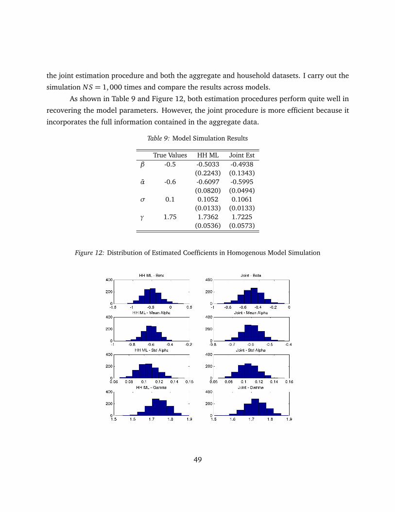
the joint estimation procedure and both the aggregate and household datasets. I carry out the
simulation NS = 1,000 times and compare the results across models.
As shown in Table 9 and Figure 12, both estimation procedures perform quite well in
recovering the model parameters. However, the joint procedure is more efficient because it
incorporates the full information contained in the aggregate data.
Table 9: Model Simulation Results
True Values HH ML Joint Estβ -0.5 -0.5033 -0.4938
(0.2243) (0.1343)α -0.6 -0.6097 -0.5995
(0.0820) (0.0494)σ 0.1 0.1052 0.1061
(0.0133) (0.0133)γ 1.75 1.7362 1.7225
(0.0536) (0.0573)
Figure 12: Distribution of Estimated Coefficients in Homogenous Model Simulation
49

B Data Appendix
B.1 Household Sample Construction
All households who buy at least one of the inside goods should be included in the household
sample. For the initial model estimation, I restrict to only the set of households who ever bought
an e-cigarette product.
B.2 Rationalizing Multiple Purchases with Discrete Choice
In some cases a household will buy multiple units of a given product or multiple different
products from the choice set in a given day (or week after aggregation). This observed behavior
is inconsistent with the discrete choice assumption of the model. For the former, I ignore
quantity and focus only on whether at least one unit was purchased. Looking at weekly HH
data, a single carton (pack) is purchased in 57% (18%) of weeks in which at least one carton
(pack) was purchased. In the latter case, I create duplicate entries for that day, and ensure that
the addiction dummy variable takes a value of 1 if at least one purchase from the previous day
is for a cigarette product.
B.3 Household Price Series Construction
In order to estimate the model, I need to fill in missing prices for days in which households
did not make a purchase and products that were not purchased. Rather than use the same
price series as the aggregate data (average price across all stores in the market), I fill in missing
prices using the last price paid by the household. Average price will capture variations in
prices that last price paid wouldn’t capture, but last price paid by a household is consistent if
households tend to buy different products. I.e. a $6 pack of expensive cigs relative to a $5
average price/pack. For days before the first purchase was made, I fill in the price of the first
purchase. If a household never purchased the product, I use the average price in stores in the
household’s county. Some households report a price per pack larger than $20+. I drop all
observations for purchases of packs over $17.
50

B.4 Aggregate Price Series Construction
A market-level price series is constructed for packs of cigarettes, cartons of cigarettes, and refill
cartridges and disposable e-cigarettes. The price series is calculated as the quantity-weighted
price of products sold in each week across all stores in a given market.
51