Advertising, Consumer Awareness and Choice:

Evidence from the U.S. Banking Industry

⇤

PRELIMINARY AND INCOMPLETE.

DO NOT CITE OR CIRCULATE WITHOUT THE AUTHORS’ PERMISSION.

Current version: July 2014

Elisabeth Honka† Ali Hortacsu‡ Maria Ana Vitorino§

Abstract

Does advertising serve to (i) increase awareness of a product, (ii) increase the likelihood thatthe product is considered carefully, or (iii) does it shift consumer utility conditional on havingconsidered it? We utilize a detailed data set on consumers’ shopping behavior and choices overretail bank accounts to investigate advertising’s e↵ect on product awareness, consideration, andchoice. Our data set has information regarding the entire “purchase funnel,” i.e., we observethe set of retail banks that the consumers are aware of, which banks they considered, andwhich banks they chose to open accounts with. We formulate a structural model that accountsfor each of the three stages of the shopping process: awareness, consideration, and choice.Advertising is allowed to a↵ect each of these separate stages of decision-making. Our modelalso endogenizes the choice of consideration set by positing that consumers undertake costlysearch. Our results indicate that advertising in this market is primarily a shifter of awareness,as opposed to consideration or choice. We view this result as evidence that advertising serves aprimarily informative role in the U.S. retail banking industry.

Keywords: advertising, banking industry, consumer search, demand estimation

JEL Classification: D43, D83, L13

⇤We thank the participants of the 2013 Marketing Science conference (Istanbul), the 2014 UT Dallas FORMSconference, the 2014 IIOC conference (Chicago) the 2014 Yale Customer Insights conference (New Haven), and seminarparticipants at Brown University for their comments. We specifically thank the discussants Sridhar Narayanan andLawrence White for the detailed comments on our paper. We are grateful to RateWatch and to an anonymousmarket research company for providing us with the data. Mark Egan provided excellent research assistance. MariaAna Vitorino gratefully acknowledges support from the Dean’s Small Grants Program at the University of MinnesotaCarlson School of Management. All errors are our own.

†University of Texas at Dallas, elisabeth.honka@utdallas.edu.‡University of Chicago and NBER, hortacsu@uchicago.edu.§University of Minnesota, vitorino@umn.edu.

1 Introduction

In his classic book, Chamberlin (1933) argued that advertising a↵ects demand because (i) it con-

veys information to consumers with regard to the existence of sellers and the prices and qualities of

products in the marketplace and (ii) it alters consumers’ wants or tastes. This led to the distinction

between the “informative” and the “persuasive” e↵ects of advertising in the economics literature

(as surveyed, for example, in Bagwell 2007). The marketing literature refines the Chamberlinian

framework by positing the “purchase funnel” framework for the consumer’s shopping process: con-

sumers first become “aware” of the existence of products; then they can choose to “consider” certain

products investigating their price and non-price characteristics carefully; and, finally, they decide

to choose one of the considered alternatives. In this framework, advertising can a↵ect each of these

three stages: “awareness,” “consideration,” and, finally, “choice.”

This paper uses detailed survey data to empirically disentangle the roles of advertising on the

di↵erent stages (awareness, consideration, and choice) of the consumer’s purchase process when

opening a bank account. More specifically, we measure how much advertising influences consumer

behavior directly as a utility shifter vs. as a way of increasing consumers’ awareness of the brand or

of inducing the consumer to consider a bank. We conduct our measurement through a fully-specified

structural model that contains the awareness-consideration-choice stages and, in particular, endoge-

nizes the “choice” of consideration set by each consumer using a costly-search framework. The value

of the structural approach is that it allows us to consider the impact of various (counterfactual)

managerial policies in a logically consistent fashion.

Our paper also contributes to our understanding of demand for retail banking products and

services, a very large and growing sector of the economy. With its $14 trillion of assets, 7,000 banks,

and more than 80,000 bank branches, the U.S. banking sector comprises a very important portion

of the “retail” economy with significant attention from regulators and policy-makers. Despite the

importance of the banking sector, structural demand analyses to date (e.g. Dick 2008, Molnar, Violi,

and Zhou 2013, Wang 2010) have only utilized aggregated market share data on deposits. There has

been very little research using detailed consumer level data to characterize consumers’ heterogeneous

response to drivers of demand. Moreover, although the banking and financial industry spends more

than $8 billion per year on advertising,1 there is little academic research that investigates the precise

way through which advertising a↵ects consumer demand in this important industry. Some recent

exceptions in the literature are Gurun, Matvos, and Seru (2013) on the marketing of mortgages and

Hastings, Hortacsu, and Syverson (2013) on retirement savings products; however, neither of these

studies can di↵erentiate between the awareness and the utility-shifting functions of advertising.

Our study is based on individual-level survey data on consumers’ (aided) awareness for banks,

the set of banks the consumer considered, and the identity of the bank the consumer decided to

open one or more new bank accounts with. In addition, we observe a nearly complete customer

profile containing information on demographics and reasons for opening a new bank account (with

1http://kantarmediana.com/intelligence/press/us-advertising-expenditures-increased-second-quarter-2013

1

their current primary bank or with a new bank) or for switching banks. We complement this data

with three additional sets of data on the retail banking industry. Data provided by RateWatch

contain information on interest rates for the most common account types for all banks over the

same time period as the first set of data. Advertising data were gathered from Kantar Media’s

Ad$pender database. Kantar tracks the number of advertisements and advertising expenditures

in national media as well as both measures of advertising in local media at the Designated Media

Area (DMA) level. Lastly, we collected information on the location of bank branches from the

Federal Deposit Insurance Corporation (FDIC).These data give us a detailed picture of consumers’

shopping and purchase processes and of the main variables a↵ecting them.

Our data show that consumers are, on average, aware of 6.8 banks and consider 2.5 banks and

that there is large variation in the size of consumers’ awareness and consideration sets. Further,

the correlation between the size of consumers’ awareness and consideration sets is low indicating a

distinct di↵erence between the two stages. This di↵erence is further reflected in the large variation

across consumers in what concerns which banks enter consumers’ awareness and consideration

sets. There are also large di↵erences in the conversion rates from awareness to consideration and

from consideration to purchase across banks. Looking at the consumers’ decision process, the

most common account types consumers shop for are checking accounts (85 percent of consumers),

savings accounts (98 percent) and credit cards (26 percent). Finally, our data also show the crucial

importance of local bank presence – i.e., bank branches – in the consumer decision process: given

that a consumer decides to consider or purchase from a bank, we find that the probability that a

bank has a local branch within 5 miles of the consumer’s home lies between 42 and 90 percent or

47 and 93 percent, respectively.

We develop a structural model of the three stages of the consumer’s purchase process: awareness,

consideration, and choice. Our model reflects the consumer’s decision process to add one or more

bank accounts to his existing portfolio and includes his costly search for information about interest

rates. Awareness is the result of bank advertising, local bank presence, and demographic factors.

A consumer searches among the banks he is aware of. Searching for information is costly for the

consumer since it takes time and e↵ort to contact financial institutions and is not viewed as pleasant

by most consumers. Thus a consumer only investigates a few banks that together represent his

consideration set and makes the final decision to open one or more new accounts with a bank from

among the ones in the considered set. Our utility-maximizing modeling approach contains all three

outcome variables: the set of banks the consumer is aware of, the consumer’s decision of which

banks to include in his consideration set given his awareness set, and the decision of which bank to

open one or more accounts with given his consideration set. To estimate our structural model we

enhance the approach developed by Honka (2014) by including the awareness stage.

We are able to disentangle the e↵ects of advertising from the e↵ects of local bank presence, as

our advertising measure does not include in-branch advertising. As expected, we find a positive

e↵ect of local bank presence on consumers’ awareness of a bank. Our results show that advertising

has a large e↵ect on consumer awareness for a bank but a↵ects consumers’ consideration and final

2

choice decisions only marginally. This suggests that, in the retail banking industry, advertising’s

primary role is to inform the consumer about the existence and availability of retail banks and

their o↵erings. This finding stands in contrast to other recent research that has also investigated

consumers’ demand for financial products. For example, Gurun, Matvos, and Seru (2013) and

Hastings, Hortacsu, and Syverson (2013) suggest a persuasive e↵ect of advertising for mortgages

and retirement savings products, respectively.

The estimates from the consideration and choice stages indicate that the average consumer

search cost rationalizing the amount of search conducted by consumers within their awareness

sets is about 9 basis points (0.09%). Our results also show that convenience is the major driver

in the consumers’ shopping and account-opening process. Convenience is captured by the fact

that consumers are more likely to open bank accounts with banks with which they already have

a relationship and that have branches located in proximity to their place of residence. Inertia

towards the consumer’s primary bank supports the convenience factor of one-stop-shopping – i.e.,

consumers only having to deal with one bank for all of their financial matters. The positive e↵ect

of local bank presence shows that, in spite of the widespread availability and convenience of online

banking, consumers still value having the possibility of talking to a bank employee in person.

The main positive result of our empirical analysis is that the role played by advertising in

the retail banking sector is largely informative as opposed to persuasive. Beyond this finding,

we will use our detailed demand side results to conduct two counterfactuals: In the first one, we

will quantify the socially optimal amount of informative advertising. In the second one, we will

investigate the e↵ects of free interest rate comparisons provided by an internet bank.

The remainder of the paper is organized as follows: In the next section, we discuss the relevant

literature. In Section 3, we describe our data. Then we introduce our model and discuss identifi-

cation in the following two sections. We present our estimation approach in Section 6 and show

our results in Section 7. In Section 8, we consider two counterfactual scenarios, the first investigat-

ing how much the observed amount of informative advertising deviates from the socially optimal

amount of informative advertising. The second counterfactual considers the scenario where one of

the banks allows consumers to compare the interest rates o↵ered by competitors. Next, we present

robustness checks and discuss limitations of our work and suggest opportunities for future work.

Finally, we conclude by summarizing our findings in the last section.

2 Relevant Literature

This paper is related to four streams of literature, namely, on advertising, multi-stage models of

consumer demand, consumer search and consumer purchase behavior for financial services.

Since Chamberlin’s (1933) seminal paper in which he described the informative and persuasive

e↵ects of advertising, several empirical researchers have tried to distinguish between these two

e↵ects of advertising in a variety of industries. For example, Ackerberg (2001) and Ackerberg (2003)

investigate the roles of advertising in the yogurt market. Narayanan, Manchanda, and Chintagunta

3

(2005), Chan, Narasimhan, and Xie (2013) and Ching and Ishihara (2012) study the pharmaceutical

market and Lovett and Staelin (2012) investigate entertainment (TV) choices. Clark, Doraszelski,

and Draganska (2009) use data on over three hundred brands and find advertising to have a positive

e↵ect on awareness but no significant e↵ect on perceived quality. Our focus is on financial products

and, more specifically, retail banking. There is little academic research that investigates the precise

way through which advertising a↵ects consumer demand for financial products. Gurun, Matvos,

and Seru (2013) and Hastings, Hortacsu, and Syverson (2013) explore the e↵ects of advertising in

the mortgage and social security markets but neither of these studies can di↵erentiate between the

awareness and the utility-shifting functions of advertising. Because we observe consumers’ (aided)

awareness of, consideration of and purchase from individual banks, we can distinguish between

advertising a↵ecting consumer’s information and advertising shifting consumer’s utility.

While it is well-known that consumers go through several stages (awareness, consideration and

choice) in their shopping process before making a purchase decision (as discussed, for example, in

Winer and Dhar 2011, p. 111), most demand side models maintain the full information assumption

that consumers are aware of and consider all available alternatives. This assumption is mostly

driven by data restrictions as information going beyond the purchase decision is rarely available to

researchers. Among the set of papers that explicitly acknowledge and model the di↵erent stages of

the consumer’s shopping process a crucial distinction relates to the data and identification strategy

used. A first group of papers models at least two stages, usually consideration and choice, and

uses purchase data for estimation purposes (e.g., Allenby and Ginter 1995, Siddarth, Bucklin, and

Morrison 1995, Chiang, Chib, and Narasimhan 1998, Zhang 2006, van Nierop et al. 2010, Terui,

Ban, and Allenby 2011). A second, smaller group of papers, also models at least two stages, but

makes use of available data on each of the shopping stages by incorporating it directly in the

estimation (e.g., Franses and Vriens 2004, Lee et al. 2005, Abhishek, Fader, and Hosanagar 2012,

De los Santos, Hortacsu, and Wildenbeest 2012 and Honka 2014).

Further distinction should be made between papers that have estimated consumers’ considera-

tion sets and papers that have also modeled how consumers form their consideration sets. Examples

of the former set of papers include Allenby and Ginter (1995), Siddarth, Bucklin, and Morrison

(1995), Chiang, Chib, and Narasimhan (1998), Zhang (2006), Goeree (2008), van Nierop et al.

(2010), while examples of the latter include Mehta, Rajiv, and Srinivasan (2003), Kim, Albu-

querque, and Bronnenberg (2010), Muir, Seim, and Vitorino (2013), Honka (2014), Honka and

Chintagunta (2014). The latter set of papers is also part of a growing body of literature on con-

sumer search. While earlier literature developed search models without actually observing search

in the data (e.g., Mehta, Rajiv, and Srinivasan 2003, Hong and Shum 2006), in the most recent

search literature, search is observed in the data either directly through data on the consumers’

consideration sets (e.g. De los Santos, Hortacsu, and Wildenbeest 2012, Honka 2014) or indirectly

through other variables (e.g., Kim, Albuquerque, and Bronnenberg 2010). In this paper, we de-

velop a structural model of all three stages of the consumer’s purchase process where consumers

form their consideration sets through search and we estimate the model using data on awareness,

4

consideration and choice.

And finally, our paper is also related to the literature examining consumer purchase behavior

for financial services and products. Hortacsu and Syverson (2004) study consumer purchase be-

havior for S&P 500 index funds and Allen, Clark, and Houde (2012) look at consumer behavior

when buying mortgages. There is also a stream of literature on consumer adoption and usage of

payment cards (e.g. Rysman 2007, Cohen and Rysman 2013, Koulayev et al. 2012, see Rysman

and Wright 2012 for an overview). Somewhat surprisingly, and despite its size and importance for

both consumers and the economy, the literature on consumer demand for retail banks and their

products is very sparse. Dick (2008) and Wang (2010) develop aggregate-level, structural models

of consumer demand for retail banks. Dick (2007) and Hirtle (2007) investigate branching struc-

tures and Dick (2007) and Molnar, Violi, and Zhou (2013) study competition in retail banking.

Similar to Dick (2008) and Wang (2010), we estimate demand for retail banks, but in contrast to

the before mentioned papers, our model describes consumer shopping and purchase behavior using

consumer-level data.

3 Data

To conduct our analysis we combine several data sets. We describe these data sets below before

turning to the presentation of our model and to the empirical results.

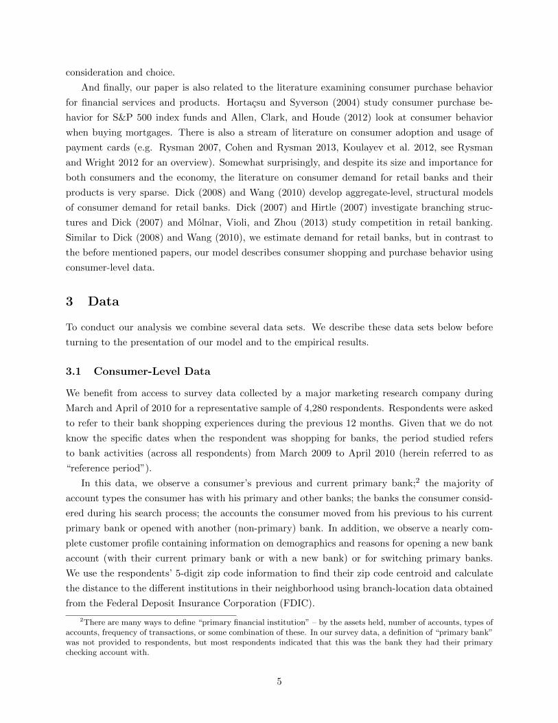
3.1 Consumer-Level Data

We benefit from access to survey data collected by a major marketing research company during

March and April of 2010 for a representative sample of 4,280 respondents. Respondents were asked

to refer to their bank shopping experiences during the previous 12 months. Given that we do not

know the specific dates when the respondent was shopping for banks, the period studied refers

to bank activities (across all respondents) from March 2009 to April 2010 (herein referred to as

“reference period”).

In this data, we observe a consumer’s previous and current primary bank;2 the majority of

account types the consumer has with his primary and other banks; the banks the consumer consid-

ered during his search process; the accounts the consumer moved from his previous to his current

primary bank or opened with another (non-primary) bank. In addition, we observe a nearly com-

plete customer profile containing information on demographics and reasons for opening a new bank

account (with their current primary bank or with a new bank) or for switching primary banks.

We use the respondents’ 5-digit zip code information to find their zip code centroid and calculate

the distance to the di↵erent institutions in their neighborhood using branch-location data obtained

from the Federal Deposit Insurance Corporation (FDIC).

2There are many ways to define “primary financial institution” – by the assets held, number of accounts, types ofaccounts, frequency of transactions, or some combination of these. In our survey data, a definition of “primary bank”was not provided to respondents, but most respondents indicated that this was the bank they had their primarychecking account with.

5

For tractability reasons, we focus on the 18 largest financial institutions in the United States

which had a combined national market share of 56 percent (measured in total deposits) in 2010.

The leftmost column in Table 1 shows the list of included banks. We drop all respondents that

have at least one institution in their consideration sets that is not among the 18 institutions listed.

Further, we also remove all respondents with invalid zip codes. This resulted in a final sample of

2, 076 consumers. To ensure that dropping consumers did not introduce a selection problem, we

compare the demographics of the initial and final set of respondents in Table 2. The descriptives

show that the final data set contains consumers with similar demographics to those in the initial

data.

=========================

Insert Table 1 about here

=========================

=========================

Insert Table 2 about here

=========================

Table 3 shows descriptive statistics for all respondents in our final sample as well as for the two

subgroups of respondents: “shoppers” (1, 832 consumers) and “non-shoppers” (244 consumers).

Shoppers are consumers who shopped and opened one or more new accounts, and non-shoppers

are consumers who neither shopped nor opened new accounts during the reference period. We

see that 61 percent of respondents are female; 65 percent are between 30 and 59 years old; 78

percent are white; 33 percent are single/divorced and 64 percent are married/with partner. With

respect to income, households are almost equally distributed among the three categories “Under

$49,999,” “$50,000 – $99,999” and “$100,000 and over” with the last category having a slightly

smaller percentage of respondents than the other two. And, finally, regarding education, 7 percent

of respondents have a high school degree or less, while the remaining 93 percent of respondents

are evenly split among the “Some College,” “College Graduate” and “Postgraduate” categories.

Looking at shoppers and non-shoppers separately, we find non-shoppers to be older and to have

lower income and less education.

=========================

Insert Table 3 about here

=========================

We also observe the number and type(s)3 of bank account(s) the consumer opened during the

reference period. Figure 1 shows the distribution of the number of account types shoppers opened

3The types of accounts considered in the survey fall into 3 groups. “Deposit accounts” include Checking, Savings,CD and Money Market Accounts. “Borrowing accounts” include credit cards, mortgages, home equity loans or homeequity lines of credit and personal loans (including auto loans and student loans). Lastly, “Investment accounts”include Mutual funds/annuities and Stocks/bonds.

6

within 2 months of switching. On average, shoppers opened 2.25 di↵erent types of accounts with a

minimum of 1 and a maximum of 10 account types. Table 4 contains the percentages of shoppers

that opened di↵erent types of accounts. The most common account types consumers shop for are

checking accounts (85 percent of consumers) followed by savings accounts (55 percent) and credit

cards (26 percent).

=========================

Insert Figure 1 about here

=========================

=========================

Insert Table 4 about here

=========================

Table 1 displays the percentages of respondents who are aware of, consider or choose a bank. The

percentage of consumers aware of a given bank ranges from around 90 percent for the largest banks

such as Bank of America and Wells Fargo/ Wachovia to around 10 percent for the smaller banks in

our data such as M&T, and Comerica Bank. Similarly, the percentage of consumers considering a

given bank varies from around 40 percent for the larger banks to around 1–2 percent for the smaller

banks. And finally, the rightmost column in Table 1 shows the percentage of consumers who chose

to open an account with each of the banks listed in the table. The purchase shares range from less

than 1 percent to more than 13 percent.

Figures 2 and 3 show histograms of the awareness and consideration set sizes, respectively.

Consumers are aware, on average, of 6.8 banks and consider 2.5 banks. There is a large variation

in the sizes of consumers’ awareness and consideration sets which range from 2 to 15 and 2 to 9,

respectively. Further, the relationship between the size of consumers’ awareness and consideration

sets is weak (see Figures 3 and 4). This suggests that there are distinct di↵erences between how the

sets are formed and that looking at one of the stages may not be enough to understand consumers’

choices.

=========================

Insert Figure 3 about here

=========================

=========================

Insert Figure 4 about here

=========================

The di↵erences between the awareness and consideration stages are further reflected in the

large variation across consumers in what concerns which specific banks enter consumers’ awareness

7

and consideration sets. There are also large di↵erences in the conversion rates from awareness to

consideration and from consideration to purchase across banks (see Table 1). For example, while

Bank of America, Chase/WaMu, M&T and TD Bank can get about 40 to 50 percent of consumers

who are aware of these banks to consider them, Capital One, Keybank and Sovereign Bank can only

get 20 to 30 percent of consumers who are aware of these banks to consider them. Similarly, while

U.S. Bank, Suntrust Bank and Citizens Bank have conversion rates between 60 and 75 percent

from consideration to purchase, the conversion rates for Bank of America, Chase/WaMu, HSBC

and WellsFargo/Wachovia lie between 30 to 40 percent. Interestingly, it is not true that banks with

the largest conversion rates from awareness to consideration also have the largest conversion rates

from consideration to purchase. For example, Bank of America has a very high convertion rate

from awareness to consideration and a very low conversion rate from consideration to purchase.

We see that the opposite is true for Comerica Bank and Keybank, for example. This holds true

even when we compare banks with similar market shares. The market shares of HSBC, Keybank,

M&T and Sovereign Bank all lie between 2 and 3 percent. But the awareness probabilities for this

set of banks range from 8 to 23 percent indicating that predicting awareness from choice (and vice

versa) is hard.

Finally, our data also show the crucial importance of local bank presence – i.e., bank branches

location – in the consumer’s decision process: given that a consumer decides to consider or purchase

from a bank, we find that the probability that that bank has a local branch within 5 miles of the

consumer’s home lies between 42 and 90 percent or 47 and 93 percent, respectively (Table 5).

=========================

Insert Table 5 about here

=========================

3.1.1 Sample Representativeness

The focus of the shopping study conducted by the marketing research company were shoppers,

i.e. consumers that opened new accounts. We correct for the over-sampling of shoppers by using

weights in the model estimation so that the results are representative and accurately reflect the

search and switching behavior of the overall U.S. population of retail banking consumers.

We re-weigh shoppers and non-shoppers in our data using information from another survey

conducted by the marketing research company. This last survey does not contain the same level of

detail as the data described in section 3.1 but has a much larger scale (around 100, 000 respondents)

and a sampling design that ensures population representativeness. This allows us to calculate the

representative weights needed for the model estimation.

3.2 Price Data

Previous papers (e.g. Dick 2008) have imputed price data from deposit revenues (in the case of

checking accounts) and from deposit expenses (in the case of savings deposits) given that data

8

on actual interest rates is typically only available from small-sample surveys. We benefit from

access to a comprehensive database with branch-level deposit product prices. These data, provided

by RateWatch, track the rates and fees o↵ered on various deposit products at the branch level.

The data are in panel format,; i.e., for the same branch and account type there are multiple

measurements over time. We focus on the data that were collected during the reference period.

We combine the price data with the individual-level data to obtain a measure of the interest

rates that each consumer faced while shopping for a bank account. From the survey data we know

which respondents have checking and savings accounts with each bank and which banks were part

of the respondents’ consideration sets. Since we do not observe what types of checking or savings

accounts respondents have, we use information on the most popular type of 2.5K savings account4

for each bank to calculate the median (over time) interest rate for each bank in each respondent’s

zip code.5 We believe that the rates calculated using this method are a good proxy for the rates

that each respondent obtained upon searching over the banks in his consideration set. Table 6

reports summary statistics for the interest rates associated with the most popular 2.5K savings

account for each bank. We also use the RateWatch information to estimate the distribution of

prices expected by the consumer prior to searching.

=========================

Insert Table 6 about here

=========================

3.3 Advertising Data

Advertising data were gathered from Kantar Media’s “Ad$pender” database. Kantar tracks adver-

tising expenditures and number of advertisements (also called “units” or “placements”6) placed in

national media (e.g., network TV and national newspapers) as well as in local media (e.g., spot TV

and local newspapers) at the Designated Media Area (DMA) level. A DMA is a geographic region

where the population can receive the same (or similar) television and radio station o↵erings.

We calculate total advertising expenditure and placements by institution and DMA over the

period from March 2009 until April 2010 (the reference period). Respondents’ locations are iden-

tified by zip code and not DMA, so we match each respondent’s zip code to a specific DMA to

find how much each bank spent on advertising in each respondent’s DMA. We add the advertising

spending at the national level to the DMA–level advertising for each bank. Table 7 reports aver-

age advertising expenditures and placements at the DMA level for each bank during the reference

period. In the estimation we focus on placements as a measure of advertising intensity. This is so

4A 2.5K savings account is a type of savings account that requires a minimum balance of $2,500 average monthlyto avoid any fees associated with the account.

5Whenever zip code data for a specific bank in a respondent’s consideration set were not available, we used datafrom branches located in adjacent zip codes.

6According to Kantar, “units” are simply the number of advertisements placed. These data are reported byKantar without any weighting (based on spot length, size, etc.).

9

that we have a measure of advertising that is independent of the cost of advertising and that thus

can be more easily compared across DMAs and banks.

In Figures 7 and 8 we display the geographic distribution of DMA-level advertising expenditures

and placements for all the banks in our sample in the reference period and across the 206 DMAs in

the U.S. The maps clearly shows that there is significant variation in advertising spending across

DMAs. This regional variation will be useful to identify the e↵ects of advertising on bank awareness

and choice.

=========================

Insert Table 7 about here

=========================

=========================

Insert Figure 7 about here

=========================

=========================

Insert Figure 8 about here

=========================

3.4 Data Limitations

While our data are well suited to study consumers’ shopping and purchase process for retail bank

accounts because we observed (aided) awareness, consideration and choice, the data have a few lim-

itations. First, our data are cross-sectional. As a consequence, our ability to control for consumer-

level unobserved heterogeneity, beyond the factors that are observable and that we use in the

estimation, is limited. Second, our data do not contain information on credit unions, which have

a significant share of the retail banking sector in the U.S. Third, our data on interest rates/prices

relies on assumptions regarding the consumer’s account size, and the timing of the account open-

ing. Hence our interest rate/price data is a proxy for the actual interest rate/price observed by the

consumers.

4 Model

Our model describes the three stages of the purchase process: awareness, consideration, and choice.

We view awareness as a passive occurrence; i.e., the consumer does not exert any costly e↵ort to

become aware of a bank. A consumer can become aware of a bank by, for example, seeing an ad

or driving by a bank branch. We model awareness as a function of banks’ advertising intensity,

local bank presence, and consumers’ demographic variables. Consideration is an active occurrence;

10

i.e., the consumer exerts e↵ort and incurs costs to learn about the interest rates and fees o↵ered

and charged by a bank, respectively. The consumer’s consideration set is thus modeled as the

outcome of a simultaneous search model given the consumer’s awareness set. And finally, purchase

is an active, but e↵ortless occurrence in which the consumer chooses the bank which gives him the

highest utility. The consumer’s purchase decision is modeled as a choice model given the consumer’s

consideration set.

4.1 Awareness

There are N consumers indexed by i = 1, . . . , N who open (an) account(s) with one of J banks

indexed by j = 1, . . . , J . Consumer i’s awareness of bank j is a function of bank fixed e↵ects &0j ,

advertising advij , demographic variables Di, local bank branch presence bij and an error term ⇠ij

and can be written as

aij = &0j + &1jadvij +Di&2 + bij&3j + ⇠ij , 8j 6= jPB, (1)

where aij is a latent awareness score. We assume that consumer i is aware of bank j if his

awareness score for bank j is larger than 0 and unaware otherwise. advij denotes consumer- and

company-specific advertising because this variable is measured using DMA-level advertising (with

the DMA being dependent on where the consumer resides). Di are observed demographic variables

(age, gender, etc.) and bij are dummy variables indicating whether there is a branch of bank j

within 5 miles of consumer i’s zip code’s centroid. ✓1 = (&0, &1j , &2, &3j) are the parameters to be

estimated. We assume that the error term ⇠ij follows an EV Type I distribution.

Note that we exclude the consumer’s primary bank jPB from the model since we assume that

consumers are aware of their primary bank. By this logic we should also exclude any other banks

the consumer has accounts with since the consumer should be aware of those banks as well. Unfor-

tunately, although the survey data contain information on whether a consumer has other accounts

other than those with his primary bank it does not have information on the identities of the banks

the consumer has (an) account(s) with.

And, lastly, note that we are not including interest rates when modeling consumers’ awareness

sets. The reason is that a consumer logically cannot have interest rate beliefs for banks he is not

aware of.

4.2 Utility Function

Consumer i0s indirect utility for company j is given by

uij = ↵j + �1pij + �2IijPB + �3advij + �4jbij + ✏ij (2)

where ✏ij is observed by the consumer, but not by the researcher. We assume ✏ij follows an EV

Type I distribution. ↵j are company-specific brand intercepts and pij denotes prices. One of the

challenges of modeling the consumers’ shopping process for retail bank accounts stems from the

11

definition of “price”. In most retail settings, price is the posted amount the consumer has to pay to

acquire a product. When it comes to retail banking, the definition of price is not as straightforward

as price can have multiple components such as fees and interest rates and consumers can have

multiple account types. For the purpose of this paper, we define “price” as the interest rate on

2.5K savings accounts.7 IijPB is a dummy variable indicating whether bank j is consumer i0s

primary bank and bij is a dummy variable indicating whether there is a branch of bank j within

5 miles of consumer i0s zip code’s centroid. ✓2 = (↵j ,�1,�2,�3,�4j) are the parameters to be

estimated.

4.3 Consideration

We model consumers’ search as in Honka (2014). Search is simultaneous, and interest rates follow

an EV Type I distribution with location parameter ⌘ and scale parameter µ. Consumers know the

distribution of interest rates in the market, but search to learn the specific interest rate a bank will

o↵er them. Given these assumptions, utility (from the consumer’s perspective) uij is an EV Type I

distributed random variable with location parameter aij = ↵j+�1⌘+�2IijPB +�3advij+�4jbij+✏ij

and scale parameter g = µ�1. A consumer’s search decision under simultaneous search depends on the

expected indirect utilities (EIU; Chade and Smith 2005). Consumer i0s EIU, where the expectation

is taken with respect to price, is then given by

E [uij ] = ↵j + �1E [p] + �2IijPB + �3advij + �4jbij + ✏ij 8j 2 Ai. (3)

Consumer i observes the EIUs for every brand he is aware of (including ✏ij). To decide which

companies to search over, consumer i ranks all companies according to their EIUs (Chade and

Smith 2005) and then picks the top k companies to search. The theory developed by Chade and

Smith (2005) on the optimality of the ranking according to EIUs only holds under the assumption

of first-order stochastic dominance among the interest rate distributions. Since we assume that

interest rates follow a market-wide distribution, the assumption is automatically fulfilled. Further,

we also need to impose a second restriction on the simultaneous search model to be able to use

Chade and Smith (2005): search costs cannot be bank-specific.

To decide on the number of companies k for which to obtain interest rate information, the

consumer calculates the net benefit of all possible search sets given the ranking of the EIUs. A

consumer’s benefit of a searched set Si is then given by the expected maximum utility among the

searched banks. Rik denotes the set of top k banks consumer i ranked highest according to their

EIUs. For example, Ri1 contains the company with the highest expected utility for consumer i, Ri2

contains the companies with the two highest expected utilities for consumer i, etc. The consumer

picks the size of his searched set Si which maximizes his net benefit of searching denoted by �ik,

i.e. expected maximum utility among the searched companies minus the cost of search

�ik = E

maxj2Rik

uij

�� kci (4)

7Henceforth we will use the terms “price” and “interest rate” interchangeably.

12

where ci denotes consumer i0s search costs. We model search costs ci as a function of a con-

stant c0, demographics and the number of account types the consumer is planning to open.8 The

consumer picks the number of searches k which maximizes his net benefit of search.

4.4 Choice

After a consumer has formed his consideration set and learned the interest rates of the considered

banks, all uncertainty is resolved. At this stage, both the consumer and the researcher observe

interest rates. The consumer then picks the company with the highest utility among the searched

companies, i.e.

j = argmaxj2Si

uij (5)

where uij now contains the actual interest rate for consumer i by bank j and Si is the set of

searched banks.

5 Identification

The identification strategy of the search model parameters follows closely Honka (2014). The

identification of the parameters capturing di↵erences in brand intercepts, the e↵ects of advertising,

price and bank branches that vary across companies is standard as in a conditional choice model.

These parameters also play a role in consumers’ consideration set decisions.

The size of a consumer’s consideration set helps pin down search costs. We can only identify a

range of search costs as it is utility-maximizing for all consumers with search costs in that range

to search a specific number of times. Beyond the fact that a consumer’s search cost lies within a

range which rationalizes searching a specific number of times, the variation in our data does not

identify a point estimate for search costs. The search cost point estimate will be identified by the

functional form of the utility function and the distributional assumption on the unobserved part of

the utility.

The base brand intercept is identified from the consumer’s decision to search or not to search.

Intuitively speaking, the option not to search and not to open (an) account(s) is the outside option

and allows us to identify the base brand intercept. So while the search cost estimate is pinned

down by the average number of searches, the base brand intercept is identified by the consumer’s

decision to search or not.

6 Estimation

The unconditional purchase probability is given by

Pij = PiAi · PiSi|Ai· Pij|Si

(6)

8The results when search costs vary with observed heterogeneity will be added to the next version of this paper.

13

where Ai is a vector of awareness probabilities for consumer i for all 18 banks. In the fol-

lowing three subsections, we discuss how each of these probabilities are estimated. Note that the

awareness probability does not have any parameters or error terms in common with the conditional

consideration and conditional purchase probabilities. Thus it can be estimated separately.

6.1 Awareness

Given our assumption on the error term ⇠ij , we estimate Equation 1 as a binary logit regression

for each bank j separately. The probability that consumer i is aware of bank j is given by

P (aij > 0) =exp (&0j + &1jadvij +Di&2 + bij&3j)

1 + exp (&0j + &1jadvij +Di&2 + bij&3j)(7)

and the probability that consumer i is aware of the J banks is denoted by

PiAi =JY

j=1

P (aij > 0) (8)

6.2 Consideration Given Awareness

We start by pointing out the crucial di↵erences between what the consumer observes and what the

researcher observes:

1. While the consumer knows the distributions of prices in the market, the researcher does not.

2. While the consumer knows the sequence of searches, the researcher only partially observes

the sequence of searches by observing which banks are being searched and which ones are not

being searched.

3. In contrast to the consumer, the researcher does not observe ✏ij .

Since the researcher does not observe the price distributions, these distributions need to be inferred

from the data. In other words, the typical assumption of rational expectations (e.g. Mehta, Rajiv,

and Srinivasan 2003, Hong and Shum 2006, Moraga-Gonzalez and Wildenbeest 2008, Honka 2014,

Honka and Chintagunta 2014) is that these distributions can be estimated from the prices observed

in the data. Given that the parameters of the price distributions are estimated, we need to account

for sampling error when estimating the other parameters of the model (see McFadden 1986).

To address the second issue, we point out that partially observing the sequence of searches

contains information that allows us to estimate the composition of consideration sets. Honka

(2014) has shown that the following condition has to hold for any searched set

minj2Si

(E [uij ]) � maxj0 /2Si

�E⇥uij0

⇤�\ �ik � �ik0 8k 6= k0 (9)

i.e. the minimum EIU among the searched brands is larger than the maximum EIU among the

non-searched brands and the net benefit of the chosen searched set of size k is larger than the net

benefit of any other search set of size k0.

14

We account for the fact that the researcher does not observe ✏ij (point 3 above) by assuming that

✏j has an EV Type I distribution with location parameter 0 and scale parameter 1 and integrating

over its distribution to obtain the corresponding probabilities with which we can compute the

likelihood function. Then the probability that a consumer picks a consideration set Si = ⌥ is

PiSi|✏ = Pr

✓minj2Si

(E [uij ]) � maxj0 /2Si

�E⇥uij0

⇤�\ �ik � �ik0 8k 6= k0

◆(10)

6.3 Purchase Given Consideration

We now turn to the purchase decision stage given consideration. The consumer’s choice probability

conditional on his consideration set is

Pij|Si,✏ =�uij � uij0 8j 6= j0, j, j0 2 Si

�(11)

where we now include the actual prices in the utility function. Note that there is a selection

issue: given a consumer’s search decision, the ✏ij do not follow an EV Type I distribution and the

conditional choice probabilities do not have a logit form. We solve this selection issue by using

SMLE when we estimate the conditional purchase probabilities.

In summary, the researcher estimates the price distributions, observes only partially the utility

rankings, and does neither observe ⇠ij in the consumer’s awareness nor ✏ij in the consumer’s utility

function. Given this, our estimable model has awareness probability given by Equation 7, con-

ditional consideration set probability given by Equation 10, and conditional purchase probability

given by Equation 11.

We maximize the joint likelihood of awareness set, consideration set, and purchase. The likeli-

hood of our model is given by

L =NY

i=1

"HY

h=1

P �ihiAi

#·

2

4Z +1

�1

LY

l=1

JY

j=1

P #iliSi|Ai,✏

· P �ijij|Si,✏

f(✏) d✏

3

5 (12)

where �ih indicates the awareness set, #il indicates the chosen consideration set, and �ij the

bank with which the consumer chooses to open an account with. ✓ = {✓1, ✓2, ci} is the set of

parameters to be estimated. Neither the consideration set probability as shown is equation (10)

nor the purchase probability as shown in equation (11) have a closed-form solution. Honka (2014)

describes how to estimate this simultaneous search model in detail, and we follow her estimation

approach.

6.4 Advertising Endogeneity

One potential concern is advertising endogeneity. For example, banks may set advertising levels

according to their branches’ specific performance e.g. in terms of customer satisfaction. Since

customer satisfaction is not observed by the researcher, but may be observed by bank management,

this can give rise to advertising endogeneity concerns.

15

We collected data on the cost of advertisements at the DMA-level and will use these advertising

costs as exogenous shifters of advertising placement decisions. Since our model is highly nonlinear,

we are considering using the control function approach in the next version of the paper.

7 Results

7.1 Awareness

We start by discussing our results on consumer awareness for retail banks. Table 8 shows the

estimates from four multivariate logit regressions: Model (A1) includes bank fixed e↵ects and

demographics and Model (A2) also includes advertising intensity. In Model (A3), we subsequently

control for bank branch presence. And, finally in Model (A4), we let the e↵ects of advertising to

be bank-specific.9

In all four models, all bank fixed e↵ects other than Bank of America in Model (A4) are signif-

icant. As expected, the big-4 banks (Bank of America, Citi, Chase, Wells Fargo) have relatively

higher brand awareness when compared to their more regional counterparts. In Model (A2), we find

a small positive coe�cient of advertising (measured in 1, 000 units/placements) which decreases in

magnitude (but still remains significant) once we control for local bank branch dummies in Model

(A3). The e↵ects of local branch presence are large and positive. In Model (A4), we see that even

after allowing for bank-specific coe�cients on advertising the e↵ects of local bank branch dummies

remain similar to the ones found in Model (A3). Further, we also see quite a bit of heterogeneity

in the e↵ects of advertising across banks. The e↵ects of advertising vary considerably in magni-

tude ranging from 0.0113 for Capital One to 1.4796 for Comerica Bank. Most interestingly, the

advertising coe�cients for the big-4 banks (Bank of America, Citi, Chase, Wells Fargo) are all

insignificant. At this point in time, we speculate that the insignificant e↵ects of advertising might

be due to diminishing returns of advertising as we observe banks which advertise more to have

smaller coe�cient estimates. We will test this hypothesis in the next version of the paper by also

including squared advertising in the awareness function.

To quantify the e↵ect of advertising, note that the average probability (across all banks and

consumers) of a consumer being aware of a bank is 32.46 percent. When advertising (measured in

1, 000 units/placements) is increased by 1 percent, the average probability (across all banks and

consumers) of a consumer being aware of a bank increases by 32.51 percent, i.e. an increase of 5 basis

points. These estimates also allow us to quantify the “brand awareness” value of the banks in terms

of advertising quantity. For example, in Model (A2), we find that Chase’s brand fixed e↵ect is 2.2458

points above Citibank’s. Using the estimated advertising coe�cient of 0.1624, this means the “brand

value gap” between Citi and BofA consists of 13, 829 advertisements (2.2458/0.1624 multiplied by

1,000). Moreover, note that the “branch presence” indicator coe�cients are between 1 to 16

9In Table 8, we show the estimation results for the awareness stage after shoppers and non-shoppers have been re-weighted to our data to be representative of the population. We also estimated our model with the non-representativesample and our results are similar.

16

times the advertising coe�cient (based on Model A4 estimates, focusing on significant coe�cients),

suggesting that the presence of a branch is worth around 1,000 to 16,000 advertisements (assuming,

of course, that the advertising e↵ect is linear throughout its domain).

=========================

Insert Table 8 about here

=========================

Finally, we also control for consumer demographics and find that the more thoroughly we control

for advertising and local bank presence, the fewer parameters associated with demographic variables

are significant. In Model (A4), only three demographics are significant: Asians and Hispanics are

aware of fewer banks than Whites and single/ divorced consumers have smaller awareness sets.

7.2 Consideration and Purchase

Models (LI-1) and (LI-2) in Table 9 show the estimates for the consideration and purchase parts

of the model. In Model (LI-2), we allow the e↵ects of local bank branches to be bank-specific.10

Similarly to the results on awareness, we find all brand intercepts and bank branch dummies to

be significant. As expected, local bank presence increases consumers’ utility for a bank with the

e↵ects ranging from 0.3839 for US Bank to 1.2999 for Keybank. Among the variables entering

consumers’ utility function, local bank presence is the second-largest utility shifter after interest

rates. Also, the estimated coe�cients for local bank presence are much larger in magnitude than

the advertising coe�cient and the coe�cient on inertia (i.e. whether the consumer switches his

primary bank). Being a consumer’s primary bank, having high interest rates on savings accounts

and local bank presence increase consumer’s utility for a bank. While significant, the coe�cient

for advertising is small and advertising is by far the smallest utility shifter. Thus we conclude that

advertising for retail banks only shifts consumer utility marginally.

=========================

Insert Table 9 about here

=========================

We find consumer search costs for retail banks (measured in interest-rate percentage points) to

be 0.09 percentage points (9 basis points) per bank searched, which translates to about $2.25 for a

2.5K account. Interestingly, this amount of search cost is comparable to other search cost estimates

in the financial products industry. For example, Hortacsu and Syverson (2004) found median search

costs to be between 7 and 21 basis points for S&P 500 index funds, which are typically purchased

by more financially sophisticated and higher-income individuals.

10In Table 9, we show the estimation results for the consideration and purchase stages after shoppers and non-shoppers have been re-weighted to our data to be representative of the population. We also estimated our modelwith the non-representative sample and our results are similar.

17

Based on the estimated coe�cient for the “Primary Bank” dummy variable, switching costs

with regard to a consumer changing his primary bank appear to be an important factor of demand

in this market. The coe�cient estimate on Primary Bank is about half of the coe�cient estimates

for local bank presence which implies that branch closures have the potential to lead to consumers

switching their primary bank.

7.3 Does Advertising have an “Informative” or a “Persuasive” Role?

To compare the magnitudes of the e↵ects of advertising across the di↵erent stages in the purchase

process, we calculate advertising elasticities for awareness and choice. Table 11 shows the results.

The average advertising elasticities for awareness and choice are 0.89 and 0.27, respectively. This

finding indicates that advertising rather a↵ects consumer awareness than choice conditional on

awareness and that the role of advertising in the U.S. retail banking industry is primarily informa-

tive. Our results are similar to those found by previous literature albeit in di↵erent categories. For

example, Ackerberg (2001) and Ackerberg (2003) find that advertising has a primarily informative

role in the Yogurt market and Clark, Doraszelski, and Draganska (2009) also show that advertising

has stronger informative e↵ects in a study of over 300 brands.

=========================

Insert Table 11 about here

=========================

Looking at the bank-specific advertising elasticities for awareness and choice, we find that the

advertising elasticities for awareness vary from 0.02 to 7.89, while the advertising elasticities for

choice conditional on awareness range from 0.00 to 1.15. For most banks, the advertising elasticity

for awareness is larger than that for choice. One important exception is Bank of America. Its

advertising elasticity for choice is about five times larger than that on awareness.11 Thus, for Bank

of America, the role of advertising is primarily persuasive.

7.4 Comparison with a Model under Full Information

In the previous sections, we developed and estimated a complete three-stage model of the consumer’s

shopping and account opening process that accounts for a consumer’s limited information. Doing

so only makes sense when limited information is an important factor in the decision-making process

and significantly influences results. To show the importance of accounting for limited information

in the retail banking sector, we compare our estimates to those obtained from a model under full

information. In the full information model, we assume consumers are aware of and consider all

banks when deciding on the bank with which they would like to open (an) account(s) with (we

also allow for an outside option). Further, consumers know the actual interest rate any bank in the

11For Keybank and Capital One, the advertising elasticity for choice is also larger than that for awareness. Butthe di↵erence in magnitudes is much smaller: In both cases, the advertising elasticity for choice is about twice aslarge as the advertising elasticity for awareness.

18

data will o↵er them. Under these assumptions, the full information model can be estimated as a

multinomial logit model. The results are shown as Model (FI) in Table 9. Compared to the results

from the model under limited information, the coe�cient estimates for local bank presence are two

to five times larger, the coe�cient estimate for primary bank is negative and, most importantly,

the coe�cient estimate on interest rates is also negative, i.e. consumers prefer savings accounts

with lower than higher interest rates, under the full information assumption.

The reason for the negative interest rate coe�cient is the following: Recall that there are 18

banks in the retail banking sector and that consumers, on average, only consider 2.5 banks. When

demand is estimated under the full information assumption, in many cases consumers do not pick

the option with the highest or one of the highest interest rates among the 18 banks. Under full

information, this behavior is attributed to the consumer being insensitive to interest rates or, in this

specific case, even preferring lower to higher interest rates (holding everything else constant). Under

limited information, the model can distinguish between the consumer not picking a bank with a

high interest rate because he does not know about it (due to not being aware of or not considering

the bank) and the consumer being insensitive to interest rates. We conclude that it is essential to

account for consumers’ limited information in the retail banking sector to get meaningful demand

estimates.

7.5 Interest Rate Elasticities

Table 10 shows the own-interest rate elasticities implied by our limited information model. The

mean interest rate elasticity across all companies is 0.03 and the bank-specific interest rate elastici-

ties vary from 0.00 to 0.09. A strong contrast is found when the interest rate elasticities calculated

under limited information are compared to those estimated under full information. The average

own-interest rate elasticity under full information is -0.01. The negative sign of the interest rate

elasticity is counterintuitive and comes from the negative interest rate coe�cient reported in Table

9 and discussed in the previous section.

=========================

Insert Table 10 about here

=========================

8 Counterfactuals

Note: We are currently working on the counterfactuals and results will be available in the next

version of the paper.

Note that our model is a partial equilibrium model. Thus any counterfactuals only capture

consequences on the demand side, i.e. we do not model interest rates or advertising spending

adjustments on the supply side. The results can be interpreted as short-run market e↵ects.

19

8.1 Welfare Analysis

While informative advertising is viewed as “good,” there is some debate about whether persuasive

advertising actually provides consumers with any “real” utility. If persuasive advertising does not

yield any real utility, then we may ask what the socially optimal amount of informative advertising is

given that there are costs to advertising. In this counterfactual, we will study three scenarios: First,

we investigate what happens to market shares if either persuasive and/or informative advertising is

shut down and interest rates are fixed. Next, we allow interest rates to adjust in the same scenarios.

And finally, assuming that persuasive advertising does not yield any real utility to consumers, we

quantify the socially optimal amount of informative advertising. We then compare this with the

observed amount of informative advertising in the U.S. retail banking industry.

8.2 Free Interest Rates Comparison

Online price comparison sites such as pricegrabber.com or pricewatch.com where consumers can

costlessly see and compare product prices from di↵erent sellers are common for many products such

as groceries, appliances, electronics, toys, furniture and many more. Price comparison sites are less

common for financial services due to their complexity. Nevertheless, some innovative and largely

internet-based companies in other financial services areas such as Progressive and Esurance for

auto insurance are showing potential customers competitive price quotes on their own website thus

allowing them to costlessly see and compare prices. In this counterfactual, we investigate the e↵ects

of the only internet bank, Capital One, newly introducing free local interest rate comparisons to

all potential customers visiting its website or bank branch, i.e. all customers who consider Capital

One.12

We investigate three di↵erent scenarios. First, we study the e↵ects of the interest rate com-

parison tool introduction by itself, i.e. without any changes to the other variables. Next, suppose

Capital One accompanied the interest rate comparison tool introduction by doubling the number

of advertisements they are showing. And finally, we investigate what the necessary increase in

advertisements would be to triple Capital One’s market share to 10 percent.

9 Robustness Checks

We conduct a variety of checks to test the robustness of our results. First, we change the radius

for the local bank branch variable in the estimation. Currently, we control for local bank presence

by including an indicator variable that reflects whether there is at least one bank branch within

5 miles of the consumer’s zip code’s centroid. We also estimated our model using an alternative

radius of 10 miles from the consumer’s zip code’s centroid for local bank presence. The results are

shown in Tables 12 for awareness and Table 13 for consideration and choice. For both awareness

and consideration and choice, we find very similar and for most significant bank branch dummies

12Capital One only had 854 bank branches in the U.S. (in 2010), with over 70 percent of them being located inthe states of New York, Texas and Louisiana.

20

slightly larger coe�cients using the 10-miles radius compared to the 5-miles radius. The estimates

for the other variables remain very similar. Thus we conclude that our results are robust to di↵erent

definitions of local bank presence.

=========================

Insert Table 12 about here

=========================

=========================

Insert Table 13 about here

=========================

Second, we also verified the robustness of our results to an alternative definition of interest

rates. The current reported results are based on interest rate data calculated using information

on the top 2.5K savings account for each bank. But we also experimented using data on all 2.5K

savings accounts that each bank has, and the results did not change significantly.

And lastly, we check the robustness of our results with respect to a di↵erent measure of ad-

vertising. In our model, we operationalize advertising as the sum of national and DMA-level

advertisements. In this robustness check, we only use the DMA-level advertising quantity in the

estimation. We find that our results are qualitatively and largely also quantitatively robust to this

alternative measure of advertising.

10 Limitations and Future Research

There are several limitations to our research. First, our model describes the consumer’s shopping

and account opening process given the consumer’s decision on account types he is considering

adding or moving, i.e. we do not model jointly the consumer’s choice of account types and the

search among banks. Our model assumes that consumers first decide which account types to

add/move and then begin the shopping process. It is left for future research to develop a model

where consumers choose several products and search at the same time that they evaluate those

products. Second, we use the interest rates for 2.5K savings account as a proxy for price. While

this is a reasonable assumption, a more precise price measure potentially self-reported by consumers

would further advance our understanding of consumers’ shopping process for bank accounts.

Third, we assume consumers have rational expectations about the distribution of interest rates

for all banks that they are aware of. A model that has information on consumer expectations for

interest rates or is able to recover them would enable researchers to test the hypothesis of rational

expectations. And lastly, more work is needed to enhance our understanding of the e↵ectiveness

of price promotions versus advertising in the retail banking industry. Advertisements stating, for

example, that consumers can get $200 for opening a new checking account as advertised by Chase,

are e↵ectively price promotions and their e↵ectiveness as compared to brand advertising is an open

question. We leave it to future research to find the answer to this question.

21

11 Conclusion

In this paper, we utilize a unique data set with detailed info on consumers’ shopping process for

banking services. Using data on awareness and consideration sets and the purchase decision, we

attempt to disentangle the informative and persuasive e↵ects of advertising in the retail banking

sector. We find advertising primarily informs consumers about the existence of banks and their

products and does not shift consumers’ utility for retail banking products. We also find that branch

presence is a very e↵ective driver of awareness and choice (upon consideration), reflecting the local

nature of banking (consistent with the fact that banks that operate mostly through the internet

have had very little penetration in the U.S.). Consumers face nontrivial search costs in this market,

equivalent to 0.09 percentage points in interest rate terms. Switching costs away from the primary

bank also appear to be an important factor of demand in this market, though with a similar order

of magnitude to local bank presence – i.e. (multiple) branch closures would easily lead to switching

to a di↵erent bank. We hope that our (still preliminary) results shed light on the drivers of demand

in this very important sector of the economy, and we hope to seek further managerial and policy

implications of our demand estimates in the near future.

22

References

Abhishek, Vibhanshu, Peter Fader, and Kartik Hosanagar (2012), “The Long Road to Online

Conversion: A Model of Multi-Channel Attribution,” Working paper, Carnegie Mellon University.

Ackerberg, Daniel A (2001), “Empirically distinguishing informative and prestige e↵ects of adver-

tising,” RAND Journal of Economics, 316–333.

Ackerberg, Daniel A. (2003), “Advertising, learning, and consumer choice in experience good mar-

kets: an empirical examination*,” International Economic Review, 44 (3), 1007–1040.

Allen, Jason, Robert Clark, and Jean-Francois Houde (2012), “Price Negotiation in Di↵erentiated

Products Markets: Evidence from the Canadian Mortgage Market,” Working Papers 12-30, Bank

of Canada.

Allenby, Greg M. and James L. Ginter (1995), “The e↵ects of in-store displays and feature ad-

vertising on consideration sets,” International Journal of Research in Marketing, 12 (1), 67 –

80.

Bagwell, Kyle (2007), The Economic Analysis of Advertising, volume 3 of Handbook of Industrial

Organization, Elsevier.

Chade, Hector and Lones Smith (2005), “Simultaneous Search,” Working paper.

Chamberlin, Edward (1933), The Theory of Monopolistic Competition: A Re-orientation of the

Theory of Value, Harvard University Press.

Chan, Tat, Chakravarthi Narasimhan, and Ying Xie (2013), “Treatment E↵ectiveness and Side

E↵ects: A Model of Physician Learning,” Management Science, 59 (6), 1309–1325.

Chiang, Jeongwen, Siddhartha Chib, and Chakravarthi Narasimhan (1998), “Markov chain Monte

Carlo and models of consideration set and parameter heterogeneity,” Journal of Econometrics,

89, 223 – 248.

Ching, Andrew T. and Masakazu Ishihara (2012), “Measuring the Informative and Persuasive Roles

of Detailing on Prescribing Decisions,” Management Science, 58 (7), 1374–1387.

Clark, C.Robert, Ulrich Doraszelski, and Michaela Draganska (2009), “The e↵ect of advertis-

ing on brand awareness and perceived quality: An empirical investigation using panel data,”

Quantitative Marketing and Economics, 7 (2), 207–236.

Cohen, Michael and Marc Rysman (2013), “Payment choice with consumer panel data,” Working

Papers 13-6, Federal Reserve Bank of Boston.

De los Santos, Babur I., Ali Hortacsu, and Matthijs R. Wildenbeest (2012), “Testing Models of

Consumer Search Using Data on Web Browsing and Purchasing Behavior,” American Economic

Review, 102 (6), 2955–80.

23

Dick, Astrid A. (2007), “Market Size, Service Quality, and Competition in Banking,” Journal of

Money, Credit and Banking, 39 (1), 49–81.

— (2008), “Demand estimation and consumer welfare in the banking industry,” Journal of Banking

& Finance, 32 (8), 1661–1676.

Franses, Philip H. and Marco Vriens (2004), “Advertising e↵ects on awareness, consideration and

brand choice using tracking data,” Working paper, Erasmus Research Institute of Management

(ERIM).

Goeree, Michelle Sovinsky (2008), “Limited information and advertising in the US personal com-

puter industry,” Econometrica, 76 (5), 1017–1074.

Gurun, Umit G., Gregor Matvos, and Amit Seru (2013), “Advertising Expensive Mortgages,”

Working paper, National Bureau of Economic Research.

Hastings, Justine S., Ali Hortacsu, and Chad Syverson (2013), “Advertising and Competition in

Privatized Social Security: The Case of Mexico,” Working paper, National Bureau of Economic

Research.

Hirtle, Beverly (2007), “The impact of network size on bank branch performance,” Journal of

Banking & Finance, 31 (12), 3782–3805.

Hong, Han and Matthew Shum (2006), “Using price distributions to estimate search costs,” The

RAND Journal of Economics, 37 (2), 257–275.

Honka, Elisabeth (2014), “Quantifying Search and Switching Costs in the U.S. Auto Insurance

Industry,” The RAND Journal of Economics, Forthcoming.

Honka, Elisabeth and Pradeep K. Chintagunta (2014), “Simultaneous or Sequential? Search Strate-

gies in the U.S. Auto Insurance Industry,” Working paper.

Hortacsu, Ali and Chad Syverson (2004), “Product Di↵erentiation, Search Costs, and Competition

in the Mutual Fund Industry: A Case Study of S&P 500 Index Funds,” The Quarterly Journal

of Economics, 119 (2), 403–456.

Kim, Jun B., Paulo Albuquerque, and Bart J. Bronnenberg (2010), “Online Demand Under Limited

Consumer Search,” Marketing Science, 29 (6), 1001–1023.

Koulayev, Sergei, Marc Rysman, Scott Schuh, and Joanna Stavins (2012), “Explaining adoption

and use of payment instruments by U.S. consumers,” Working paper, Federal Reserve Bank of

Boston.

Lee, Jonathan, J. Han, C. Park, and Pradeep K. Chintagunta (2005), “Modeling pre-di↵usion

process with attitudinal trackings and expert ratings: trackings and expert ratings: Forecasting

opening weekend box-o�ce,” Working paper.

24

Lovett, Mitchell J. and Richard Staelin (2012), “The Role of Paid and Earned Media in Building

Entertainment Brands: Reminding, Informing, and Enhancing Enjoyment,” Working paper,

Simon School of Business – University of Rochester.

McFadden, Daniel (1986), “The Choice Theory Approach to Market Research,” Marketing Science,

5 (4), 275–297.

Mehta, Nitin, Surendra Rajiv, and Kannan Srinivasan (2003), “Price Uncertainty and Consumer

Search: A Structural Model of Consideration Set Formation,” Marketing Science, 22 (1), 58–84.

Molnar, Jozsef, Roberto Violi, and Xiaolan Zhou (2013), “Multimarket contact in Italian retail

banking: Competition and welfare,” International Journal of Industrial Organization, 31 (5),

368 – 381.

Moraga-Gonzalez, Jose L. and Matthijs R. Wildenbeest (2008), “Maximum likelihood estimation

of search costs,” European Economic Review, 52 (5), 820–848.

Muir, David M., Katja Seim, and Maria Ana Vitorino (2013), “Price Obfuscation and Consumer

Search: An Empirical Analysis,” Working paper.

Narayanan, Sridhar, Puneet Manchanda, and Pradeep K. Chintagunta (2005), “Temporal Di↵er-

ences in the Role of Marketing Communication in New Product Categories,” Journal of Marketing

Research, 42 (3), 278–290.

Rysman, Marc (2007), “An Empirical Analysis of Payment Card Usage,” The Journal of Industrial

Economics, 55 (1), 1–36.

Rysman, Marc and Julian Wright (2012), “The Economics of Payment Cards,” Working paper,

Boston University.

Siddarth, S., Randolph E. Bucklin, and Donald G. Morrison (1995), “Making the Cut: Modeling

and Analyzing Choice Set Restriction in Scanner Panel Data,” Journal of Marketing Research,

32 (3), pp. 255–266.

Terui, Nobuhiko, Masataka Ban, and Greg M. Allenby (2011), “The E↵ect of Media Advertising

on Brand Consideration and Choice,” Marketing Science, 30 (1), 74–91.

van Nierop, Erjen, Bart J. Bronnenberg, Richard Paap, Michel Wedel, and Philip Hans Franses

(2010), “Retrieving Unobserved Consideration Sets from Household Panel Data,” Journal of

Marketing Research, 47 (1), pp. 63–74.

Wang, Hui (2010), “Consumer Valuation of Retail Networks: Evidence from the Banking Industry,”

Working paper, Peking University.

Winer, Russel S. and Ravi Dhar (2011), Marketing Management, Upper Saddle River, NJ: Prentice

Hall, 4th edition edition.

25

Zhang, Jie (2006), “An Integrated Choice Model Incorporating Alternative Mechanisms for Con-

sumers’ Reactions to In-Store Display and Feature Advertising,” Marketing Science, 25 (3), pp.

278–290.

26

Tables and Figures

Figure 1: Number of Accounts Opened

Figure 2: Size of awareness sets

27

Figure 3: Size of shoppers’ consideration sets

Figure 4: Awareness vs Consideration (Shoppers only)

28

Figure 5: Size of awareness sets

Figure 6: Awareness vs Consideration (Shoppers only)

29

Figure 7: Geographic Distribution of Banks’ DMA-level Advertising (Expenditures)

This map displays the spatial distribution of DMA-level advertising expenditure by banks in the 206 DMAs across

the U.S. over the reference period. Areas in white correspond to DMAs for which Kantar Media does not collect

data. Advertising numbers in the legend are represented in thousands.

Figure 8: Geographic Distribution of Banks’ DMA-level Advertising (Placements)

This map displays the spatial distribution of DMA-level number of advertising placements by banks in the 206 DMAs

across the U.S. over the reference period. Areas in white correspond to DMAs for which Kantar Media does not

collect data.

30

Table 1: Share of respondents that were Aware/Considered/Chose each Bank (%)

This table presents the percentage of respondents in the sample that were Aware, Considered or Chose each of the

institutions listed.

Institution Aware Considered Chose

BB&T 17.15 5.44 3.13Bank Of America 95.18 44.27 12.52Capital One 31.89 6.55 3.32Chase/WaMu 73.94 32.18 12.62Citibank 63.87 17.92 7.27Citizens Bank 25.24 7.71 4.53Comerica Bank 10.98 1.93 0.87Fifth Third Bank 25.39 7.80 3.71HSBC 21.53 7.56 3.03Keybank 24.18 6.12 2.99M&T 8.62 4.19 2.31PNC/National City Bank 34.92 11.03 4.67Regions Bank 21.10 5.97 3.08Sovereign Bank 17.68 4.82 2.26Suntrust Bank 31.12 11.66 7.61TD Bank 21.48 8.96 4.05U.S. Bank 31.21 13.01 8.33Wells Fargo/Wachovia 87.24 34.39 13.68

31

Table 2: Demographics for full and selected samples

This table compares the demographics of the respondents in the selected sample with all of the survey respondents.

Columns “All Respondents” and “Selected Sample” report the percentage of respondents in each of the demographic

groups for all of the survey respondents and for the selected sample respectively.

Data setAll Respondents Selected Sample

(n = 4, 246) (n = 2, 076)% %

GenderFemale 60.0 60.8Male 40.0 39.2Age19-29 17.0 17.930-44 30.4 32.345-59 34.0 32.460+ 18.7 17.4Household IncomeUnder $49,999 36.5 35.5$50,000-$99,999 38.0 38.2$100,000 and over 25.5 26.3RaceWhite 81.3 78.1Black 5.0 5.6Asian 7.5 9.3Hispanic 3.9 5.0Other 2.3 2.0EducationHigh school or less 8.5 7.2Some College 32.2 31.0College graduate 29.4 31.4Postgraduate 29.9 30.4Marital StatusSingle/Divorced 33.4 33.3Married/Partner 63.7 64.5Widowed 2.9 2.2RegionNew England 5.6 6.5MidAtlantic 22.9 28.3Midwest 10.5 6.7North Central 10.9 8.8Southeast 8.1 8.0South Central 4.1 3.1Texas 4.1 4.6Florida 8.8 10.8Southwest 6.3 5.9Northwest 4.3 4.5California 12.8 12.7Other 1.6 0.132

Table 3: Demographics by Respondent Type

This table reports descriptive statistics for all respondents in our final sample as well as for the two subgroups

of respondents: “shoppers” (1,832 consumers) and “non-shoppers” (244 consumers). Shoppers are consumers who

opened one or more new accounts and non-shoppers are consumers who did not open new accounts during the

reference period.

Respondent TypeShopper Non Shopper All

% % %GenderFemale 60.9 59.8 60.8Male 39.1 40.2 39.2Age19-29 19.6 5.3 17.930-44 34.2 17.6 32.345-59 30.8 43.9 32.460+ 15.3 33.2 17.4Household IncomeUnder $49,999 34.0 47.1 35.5$50,000-$99,999 38.9 32.8 38.2$100,000 and over 27.1 20.1 26.3RaceWhite 76.9 86.9 78.1Black 5.8 3.7 5.6Asian 10.0 3.7 9.3Hispanic 5.4 2.0 5.0Other 1.8 3.7 2.0EducationHigh school or less 6.4 12.7 7.2Some College 30.5 35.2 31.0College graduate 32.0 26.2 31.4Postgraduate 31.1 25.8 30.4Marital StatusSingle/Divorced 33.7 30.7 33.3Married/Partner 64.3 65.6 64.5Widowed 2.0 3.7 2.2RegionRegionNew England 6.8 4.1 6.5MidAtlantic 29.3 20.5 28.3Midwest 5.6 15.6 6.7North Central 8.2 12.7 8.8Southeast 8.2 6.6 8.0South Central 2.8 5.7 3.1Texas 4.5 5.3 4.6Florida 11.2 7.8 10.8Southwest 5.8 6.6 5.9Northwest 4.5 4.5 4.5California 12.9 10.7 12.7Other 0.2 0.0 0.1

33

Table 4: Account types opened (Shoppers only)

This table shows, for the subsample of shoppers, the types of new accounts opened during the reference period.

% Respondents % RespondentsAccount type Opening Account type Opening

Deposit Accounts Borrowing AccountsChecking 85.10 Credit Card 25.87Savings 57.86 Mortgage 9.01Certificate of Deposit 11.74 Home Equity Loan 6.28Money Market Account 12.45 Personal Loan 8.02Investment AccountsMutual Funds 4.69Stocks/Bonds 4.26

Table 5: Respondents with bank branches within 5 miles of their home (Shoppersonly)

This table reports the percentage of shoppers in the sample with bank branches within 5 miles of their home conditional

on them having Considered/Chosen each of the institutions listed.

Institution Considered Chosen

BB&T 84.82 82.81Bank Of America 85.52 86.26Capital One 69.63 67.65Chase/WaMu 88.08 90.58Citibank 69.92 78.38Citizens Bank 60.00 60.71Comerica Bank 86.84 87.50Fifth Third Bank 80.39 85.29HSBC 42.38 47.37Keybank 85.25 91.23M&T 84.81 85.00PNC/National City Bank 86.18 88.24Regions Bank 88.33 91.67Sovereign Bank 78.95 80.95Suntrust Bank 86.02 87.50TD Bank 90.76 92.68U.S. Bank 82.00 88.24Wells Fargo/Wachovia 88.65 91.44

34

Table 6: Interest Rates by Institution

This table reports summary statistics for the interest rates associated with the most popular 2.5K savings accounts

for each bank. These rates proxy for the actual rates that each respondent obtained upon searching over the banks in

his consideration set. Interest rates statistics are calculated using banks in respondents consideration sets and based

on respondents’ zip codes. N is the number of respondents that considered a given bank.

Institution mean sd min max N

BB&T 0.050 0.000 0.050 0.050 113Bank Of America 0.100 0.000 0.100 0.100 919Capital One 1.101 0.439 0.050 1.290 136Chase/WaMu 0.010 0.000 0.010 0.010 668Citibank 0.290 0.169 0.250 1.000 372Citizens Bank 0.050 0.000 0.050 0.050 160Comerica Bank 0.050 0.000 0.050 0.050 40Fifth Third Bank 0.200 0.000 0.200 0.200 162HSBC 0.050 0.000 0.050 0.050 157Keybank 0.050 0.000 0.050 0.050 127M&T 0.050 0.000 0.050 0.050 87PNC/National City Bank 0.050 0.000 0.050 0.050 136Regions Bank 0.100 0.000 0.100 0.100 124Sovereign Bank 0.100 0.000 0.100 0.100 100Suntrust Bank 0.050 0.000 0.050 0.050 242TD Bank 0.100 0.000 0.100 0.100 186U.S. Bank 0.100 0.000 0.100 0.100 270Wells Fargo/Wachovia 0.046 0.007 0.030 0.050 345

35

Table 7: DMA-Level Advertising Expenditures (dols000) and Placements by Bank

This table shows average advertising expenditures and average number of placements (also called “units”) by bank.

It includes Spot TV, Newspapers, National Spot Radio, Internet Display, Outdoor at DMA-level. The averages are

taken by dividing the total advertising expenditures/placements at the DMA-level over the entire reference period

by the number of DMAs in which each bank had some advertising activity.

Institution Average per DMA Number of DMAsExpenditure Units

BB&T 207.0 188.9 23Bank Of America 424.0 1859.0 101Capital One 432.2 895.9 97Chase/WaMu 1039.7 1376.0 98Citibank 654.4 333.2 99Citizens Bank 258.2 234.5 99Comerica Bank 336.2 271.2 16Fifth Third Bank 797.7 1526.3 30HSBC 209.5 286.0 97Keybank 415.6 1464.2 29M&T 390.2 615.4 14PNC/National City Bank 525.6 770.6 99Regions Bank 254.2 353.4 43Sovereign Bank 117.0 154.4 65Suntrust Bank 336.3 501.7 83TD Bank 848.5 810.2 43U.S. Bank 154.1 183.2 79Wells Fargo/Wachovia 433.2 1084.7 101

36

Table 8: Results from Awareness Stage

This table reports the results from four di↵erent model specifications for the Awareness stage. Panel A reports the

Brand, Branches and Advertising Parameters and Panel B reports the parameters associated with the demographic

variables. All four models include bank-specific fixed e↵ects.“Branch presence” is operationalized as a dummy variable

that captures whether there is a branch of a given bank present within 5-miles of each respondent zip-code centroid.

Advertising corresponds to the number of DMA placements. Advertising is not included in model (A1) and in Model

(A4) is allowed to have coe�cients that are bank-specific. The omitted demographic categories are Married/Partner,

White, Income below 50k and High school or less for the variables Marital Status, Race, Income and Education,

respectively. Standard-errors are reported in parentheses under coe�cient estimates. (**) and (*) denote statistical

significance for 5% and 10% levels respectively.

Panel A: Brand, Branches and Advertising Parameters

(A1) (A2) (A3) (A4)Brand Brand Brand Branch Brand Branch Advert

presence presence

Bank of America -1.530** -23.109** -9.997** 0.385 -11.726 0.076 0.355(0.257) (1.201) (1.005) (0.301) (7.216) (0.055) (0.315)

BB&T -5.141** -5.363** -5.475** 1.149** -5.424** 0.300 1.147**(0.488) (0.498) (0.512) (0.201) (0.512) (0.540) (0.227)

Citibank -2.399** -7.171** -4.709** 1.620** -4.755** 0.064 1.615**(0.249) (0.364) (0.340) (0.165) (1.244) (0.040) (0.175)

Citizens Bank -3.806** -6.846** -5.687** 1.732** -15.985** 0.666** 1.434**(0.350) (0.398) (0.403) (0.215) (2.295) (0.132) (0.225)

Comerica -5.010** -4.882** -5.817** 2.472** -6.821** 1.480** 1.522**(0.556) (0.545) (0.581) (0.206) (0.632) (0.198) (0.238)

Fifth Third -3.640** -4.130** -5.031** 2.919** -5.321** 0.453** 2.198**(0.339) (0.349) (0.399) (0.213) (0.413) (0.078) (0.240)

HSBC -4.028** -9.118** -6.022** 1.400** -17.702** 0.392** 0.953**(0.380) (0.472) (0.453) (0.228) (3.160) (0.089) (0.268)

Chase -3.525** -4.925** -4.209** 0.602** -4.078** 0.046 0.654**(0.257) (0.273) (0.282) (0.136) (0.377) (0.034) (0.167)

Keybank -3.083** -3.457** -4.225** 2.742** -4.389** 0.222** 2.429**(0.311) (0.319) (0.347) (0.179) (0.354) (0.050) (0.202)

M&T -7.354** -8.218** -8.540** 0.841** -9.246** 0.822** 0.677**(0.711) (0.753) (0.785) (0.260) (0.827) (0.171) (0.267)

PNC/N. City Bank -3.955** -19.999** -10.709** 1.582** -8.330** 0.039 1.630**(0.295) (0.930) (0.774) (0.147) (2.677) (0.027) (0.153)

Regions -4.266** -5.041** -5.516** 2.360** -6.475** 0.300** 1.554**(0.398) (0.406) (0.438) (0.199) (0.482) (0.035) (0.225)

Sovereign -4.693** -4.891** -5.468** 1.912** -5.529** 0.108* 1.832**(0.422) (0.415) (0.450) (0.216) (0.484) (0.065) (0.230)

SunTrust -3.401** -3.907** -5.131** 4.048** -6.484** 0.898** 2.613**(0.329) (0.338) (0.393) (0.267) (0.476) (0.134) (0.334)

TD -4.662** -5.809** -6.556** 2.406** -6.964** 0.131** 2.077**(0.406) (0.408) (0.467) (0.236) (0.554) (0.038) (0.283)

US Bank -2.491** -3.013** -4.596** 2.871** -5.525** 0.366** 2.819**(0.306) (0.311) (0.363) (0.183) (0.512) (0.123) (0.192)

Wells Fargo/Wachovia -3.314** -7.087** -5.288** 0.933** -5.707** 0.081** 0.918**(0.260) (0.335) (0.339) (0.190) (0.732) (0.032) (0.202)

Capital One -3.694** -10.427** -6.839** 1.586** -4.781** 0.011 2.446**(0.310) (0.491) (0.456) (0.264) (0.465) (0.008) (0.279)

Advertising 0.162** 0.063**(0.009) (0.007)

37

Table 8: Results from Awareness Stage (cont.)

Panel B: Demographics’ Parameters

(A1) (A2) (A3) (A4)

Gender – Male 0.002 -0.004 -0.044 -0.045(0.038) (0.038) (0.041) (0.041)

Age -0.001 0.000 0.001 0.001(0.001) (0.001) (0.002) (0.002)

Marital Status

Single/ Divorced 0.004 -0.033 -0.090* -0.094**(0.043) (0.043) (0.046) (0.047)

Widow -0.110 -0.167 -0.163 -0.154(0.123) (0.126) (0.133) (0.135)

Race

Black -0.059 -0.063 -0.086 -0.103(0.080) (0.081) (0.087) (0.088)

Asian -0.101 -0.166** -0.235** -0.235**(0.067) (0.069) (0.073) (0.074)

Hispanic -0.140 -0.213** -0.275** -0.279**(0.088) (0.091) (0.097) (0.097)

Other -0.062 -0.096 -0.197 -0.188(0.130) (0.133) (0.141) (0.142)

Income

Income 50k - 100k 0.110** 0.050 0.040 0.029(0.044) (0.045) (0.048) (0.048)

Income above 100k 0.163** 0.093* 0.030 0.027(0.052) (0.053) (0.056) (0.057)

Education

Some College 0.072 0.082 0.033 0.059(0.075) (0.076) (0.080) (0.081)

College Degree 0.138* 0.141* 0.005 0.027(0.076) (0.077) (0.082) (0.083)

Adv. Degree 0.133* 0.130* -0.022 -0.002(0.077) (0.078) (0.083) (0.083)

* p < 0.10; ** p < 0.05

38

Table 9: Results from Consideration and Purchase Stages

This table reports the results from three di↵erent model specifications for the Consideration and Purchase stages.

Specification (FI) corresponds to a Full Information Model, equivalent to a traditional multinomial logit model, in

which consumers are assumed to be aware and consider all banks and know what are banks’ actual interest rates

without engaging in search. Specifications (LI) correspond to models that account for consumers’ Limited Information.

In model (LI-1) branch presence is operationalized as a dummy variable that captures whether there is a branch of

a given bank present within 5-miles of each respondent zip-code centroid and in model (LI-2) branch coe�cients are

allowed to be bank-specific. Standard-errors are reported in parentheses under coe�cient estimates. (**) and (*)

denote statistical significance for 5% and 10% levels respectively.

(FI) (LI-1) (LI-2)Brand Branches Brand Brand Branches

Bank of America -2.266** 1.661** -3.259** -3.668** 0.682**(0.583) (0.212) (0.121) (0.056) (0.169)

BB&T -2.694** 3.339** -1.914** -1.926** 0.920**(0.311) (0.339) (0.064) (0.244) (0.278)

Citibank -1.793** 2.612** -2.316** -2.608** 1.133**(0.230) (0.209) (0.072) (0.160) (0.175)

Citizens Bank -1.731** 2.271** -1.801** -1.826** 0.797**(0.197) (0.236) (0.070) (0.197) (0.246)

Comerica -4.436** 4.091** -2.712** -3.191* 1.435(0.706) (0.755) (0.153) (1.707) (1.710)

Fifth Third -2.760** 3.494** -2.209** -2.034** 0.685**(0.329) (0.349) (0.083) (0.265) (0.284)

HSBC -2.038** 2.115** -1.848** -1.781** 0.462*(0.233) (0.274) (0.066) (0.215) (0.258)

Chase -1.657** 2.503** -1.951** -2.261** 1.237**(0.234) (0.237) (0.061) (0.189) (0.191)

Keybank -3.468** 4.001** -2.215** -2.563** 1.300**(0.453) (0.473) (0.080) (0.271) (0.301)

M&T -3.321** 3.685** -1.567** -1.475** 0.826(0.415) (0.449) (0.167) (0.684) (0.725)

PNC/N. City Bank -3.373** 2.828** -3.028** -3.526** 0.976**(0.475) (0.342) (0.060) (0.198) (0.230)

Regions -3.509** 4.248** -2.183** -2.409** 1.110**(0.454) (0.474) (0.089) (0.339) (0.359)

Sovereign -3.037** 3.329** -2.101** -1.819** 0.469(0.362) (0.400) (0.084) (0.370) (0.392)

SunTrust -2.177** 3.884** -1.688** -1.861** 1.126**(0.241) (0.256) (0.096) (0.397) (0.404)

TD -3.258** 3.859** -1.819** -1.687** 0.685*(0.416) (0.429) (0.111) (0.349) (0.358)

US Bank -2.073** 3.039** -1.910** -1.445** 0.384(0.250) (0.259) (0.086) (0.265) (0.277)

Wells Fargo/Wachovia -1.803** 2.439** -2.263** -2.680** 1.298**(0.261) (0.248) (0.069) (0.184) (0.188)

Capital One -2.222** 2.706** -2.622** -2.672** 0.538**(0.407) (0.298) (0.119) (0.201) (0.228)

Other parameters

Primary Bank -0.763** 0.422** 0.415**(0.090) (0.038) (0.060)

Interest Rates -0.107 0.950** 0.982**(0.276) (0.163) (0.230)

Advertising 0.009** 0.009** 0.014**(0.004) (0.001) (0.006)

Bank Branches 0.924**(0.045)

Search Cost Constant 0.001** 0.001**(0.000) (0.000)

39

Table 10: Interest Rate Elasticities

This table reports the price (i.e. interest rate) elasticities that correspond to the model estimates reported in Table

9. Specification (FI) corresponds to a Full Information Model, equivalent to a traditional multinomial logit model,

in which consumers are assumed to be aware and consider all banks and know what are banks’ actual interest

rates without engaging in search. Specification (LI-2) corresponds to a model that account for consumers’ Limited

Information in which branch presence is operationalized as a dummy variable that captures whether there is a branch

of a given bank present within 5-miles of each respondent zip-code centroid. Elasticities are calculated for each

respondent and bank and then averaged across respondents.

(FI) (LI-2)Brand

Bank of America -0.01 0.06BB&T 0.00 0.03Citibank -0.03 0.18Citizens Bank 0.00 0.03Comerica -0.01 0.04Fifth Third -0.02 0.12HSBC -0.01 0.03Chase 0.00 0.01Keybank 0.00 0.03M&T 0.00 0.03PNC/N. City Bank 0.00 0.02Regions -0.01 0.06Sovereign -0.01 0.07SunTrust 0.00 0.03TD -0.01 0.06US Bank -0.01 0.06Wells Fargo/Wachovia 0.00 0.02Capital One -0.10 0.48Average -0.01 0.07

40

Table 11: Advertising Elasticities

This table reports the advertising elasticities that correspond to the model estimates reported in Tables 8 and 9.

Elasticities are calculated for each respondent and bank and then averaged across respondents.

Awareness Choice

(4) (LI-2)Brand

Bank of America 0.22 1.15BB&T 0.02 0.00Citibank 0.73 0.28Citizens Bank 2.69 0.15Comerica 0.14 0.02Fifth Third 0.04 0.03HSBC 7.89 0.34Chase 0.14 0.08Keybank 0.02 0.04M&T 0.06 0.01PNC/N. City Bank 0.85 0.84Regions 0.27 0.08Sovereign 0.10 0.04SunTrust 0.52 0.03TD 0.22 0.09US Bank 1.45 0.03Wells Fargo/Wachovia 0.23 0.20Capital One 0.17 0.36Average 0.89 0.27

41

Table 12: Results from Awareness Stage - Robustness

This table reports the results of robustness checks for two of the Awareness stage model results shown in table 8.

Here “Branch presence” is operationalized as a dummy variable that captures whether there is a branch of a given

bank present within 10-miles (as opposed to 5-miles) of each respondent zip-code centroid. Panel A reports the

Brand, Branches and Advertising Parameters and Panel B reports the parameters associated with the demographic

variables. Standard-errors are reported in parentheses under coe�cient estimates. (**) and (*) denote statistical

significance for 5% and 10% levels respectively.

Panel A: Brand, Branches and Advertising Parameters

(A3-R) (A4-R)Brand Branch Brand Branch Advert

presence presence

Bank of America -8.024** 0.150 -13.291* 0.068 0.090(0.998) (0.328) (7.169) (0.341) (0.054)

BB&T -5.560** 1.297** -5.567** 1.304** 0.265(0.518) (0.224) (0.518) (0.249) (0.534)

Citibank -4.464** 1.753** -4.620** 1.731** 0.055(0.341) (0.161) (1.203) (0.169) (0.039)

Citizens Bank -5.588** 1.709** -15.958** 1.398** 0.658**(0.407) (0.205) (2.293) (0.215) (0.132)

Comerica -6.202** 2.575** -6.929** 1.365** 1.492**(0.594) (0.224) (0.629) (0.273) (0.214)

Fifth Third -4.966** 2.812** -5.310** 2.079** 0.476**(0.394) (0.200) (0.410) (0.227) (0.078)

HSBC -5.685** 1.381** -17.160** 0.991** 0.373**(0.453) (0.212) (3.174) (0.248) (0.089)

Chase -4.143** 0.629** -4.203** 0.609** 0.058*(0.285) (0.138) (0.374) (0.164) (0.033)

Keybank -4.414** 2.541** -4.557** 2.205** 0.218**(0.350) (0.163) (0.357) (0.189) (0.050)

M&T -8.659** 0.995** -9.533** 0.870** 0.873**(0.803) (0.317) (0.851) (0.324) (0.172)

PNC/N. City Bank -9.666** 1.881** -5.298** 1.990** 0.006(0.764) (0.158) (2.395) (0.166) (0.024)

Regions -5.846** 2.801** -6.588** 1.943** 0.256**(0.447) (0.218) (0.485) (0.258) (0.037)

Sovereign -5.701** 2.136** -5.672** 2.134** 0.055(0.457) (0.223) (0.488) (0.247) (0.068)

SunTrust -5.337** 4.295** -6.492** 2.959** 0.778**(0.404) (0.271) (0.480) (0.355) (0.141)

TD -6.549** 2.596** -6.788** 2.335** 0.097**(0.471) (0.247) (0.546) (0.314) (0.040)

US Bank -5.078** 3.280** -5.897** 3.220** 0.321**(0.384) (0.204) (0.529) (0.213) (0.126)

Wells Fargo/Wachovia -5.128** 1.053** -5.789** 1.029** 0.079**(0.347) (0.200) (0.722) (0.214) (0.031)

Capital One -6.405** 1.956** -4.684** 2.618** 0.007(0.453) (0.242) (0.463) (0.257) (0.008)

Advertising 0.049**(0.007)

42

Table 12: Results from Awareness Stage - Robustness (cont.)

Panel B: Demographics’ Parameters

(A3-R) (A4-R)

Gender – Male -0.036 -0.037(0.041) (0.041)

Age 0.001 0.000(0.002) (0.002)

Marital Status

Single/ Divorced -0.095** -0.101**(0.047) (0.047)

Widow -0.179 -0.162(0.136) (0.137)

Race

Black -0.142 -0.155*(0.088) (0.088)

Asian -0.260** -0.258**(0.073) (0.074)

Hispanic -0.334** -0.326**(0.097) (0.098)

Other -0.224 -0.207(0.141) (0.142)

Income

Income 50k - 100k 0.005 -0.002(0.048) (0.048)

Income above 100k 0.020 0.024(0.057) (0.057)

Education

Some College 0.084 0.107(0.081) (0.082)

College Degree 0.069 0.088(0.083) (0.083)

Adv. Degree 0.040 0.052(0.083) (0.084)

* p < 0.10; ** p < 0.05

43

Table 13: Results from Consideration and Purchase Stages - Robustness

This table reports the results of robustness checks for three of the Consideration and Purchase stages model results

shown in table 9. Here, “Branch presence” is operationalized as a dummy variable that captures whether there

is a branch of a given bank present within 10-miles (as opposed to 5-miles) of each respondent zip-code centroid.

Standard-errors are reported in parentheses under coe�cient estimates. (**) and (*) denote statistical significance

for 5% and 10% levels respectively.

(FI-R) (LI-1-R) (LI-2-R)Brand Branches Brand Brand Branches

Bank of America -2.213** 1.754** -3.724** -3.107** 0.749**(0.595) (0.240) (0.199) (0.146) (0.126)

BB&T -3.130** 3.724** -2.072** -2.236** 1.171**(0.385) (0.406) (0.198) (0.158) (0.184)

Citibank -1.849** 2.489** -2.470** -2.406** 0.955**(0.239) (0.218) (0.096) (0.118) (0.122)

Citizens Bank -1.768** 2.184** -1.997** -1.784** 0.694**(0.203) (0.239) (0.149) (0.125) (0.153)

Comerica -4.412** 3.744** -2.812** -2.474** 0.579*(0.711) (0.759) (0.135) (0.304) (0.342)

Fifth Third -3.454** 4.101** -2.315** -1.988** 0.584(0.456) (0.469) (0.128) (0.386) (0.398)

HSBC -1.988** 1.712** -2.085** -1.619** 0.352*(0.235) (0.272) (0.158) (0.164) (0.208)

Chase -2.080** 2.849** -2.075** -2.355** 1.298**(0.301) (0.304) (0.096) (0.151) (0.153)

Keybank -5.027** 5.385** -2.355** -3.247** 1.960**(1.002) (1.010) (0.131) (0.143) (0.165)

M&T -5.082** 5.344** -1.774** -2.161* 1.456(1.003) (1.015) (0.562) (1.254) (1.262)

PNC/N. City Bank -3.669** 3.209** -3.394** -3.029** 0.873**(0.527) (0.429) (0.258) (0.284) (0.284)

Regions -15.837 16.500 -2.356** -2.895** 1.540**(212.959) (212.959) (0.162) (0.199) (0.208)

Sovereign -3.997** 4.224** -2.254** -2.005** 0.589*(0.582) (0.603) (0.095) (0.298) (0.306)

SunTrust -2.926** 4.680** -1.810** -2.205** 1.471**(0.341) (0.351) (0.182) (0.365) (0.370)

TD -4.331** 4.877** -1.917** -1.616** 0.636(0.711) (0.719) (0.123) (0.452) (0.469)

US Bank -2.716** 3.599** -2.023** -1.581** 0.491**(0.343) (0.349) (0.086) (0.236) (0.237)

Wells Fargo/Wachovia -2.203** 2.804** -2.405** -2.917** 1.602**(0.327) (0.316) (0.113) (0.152) (0.154)

Capital One -2.592** 2.943** -2.849** -2.423** 0.571**(0.418) (0.315) (0.101) (0.146) (0.195)

Other parameters

Primary Bank -0.784** 0.460** 0.461**(0.090) (0.046) (0.042)

Interest Rates 0.047 0.872** 0.920**(0.268) (0.294) (0.194)

Advertising 0.008* 0.012** 0.008**(0.004) (0.001) (0.001)

Bank Branches 0.963**(0.082)

Search Cost Constant 0.001** 0.001(0.000) (0.000)

44