1

Economic Valuation of Storm Protection Function: A case Study of Mangrove Forest of Orissa and 1999 Super Cyclone.

Saudamini Das

Institute of Economic Growth, Delhi.

Supervisor: - Prof. Kanchan Chopra.

Sponsoring Organization: - South Asian Network foe Development and

Environmental Economics (SANDEE).

Advisor at SANDEE: - Prof. Jeffery R. Vincent.

BACK GROUND OF THE STUDY

• Super Cyclone of Oct,1999 in state of Orissa of India.

• Tremendous loss of lives and properties.

• Wide reporting in national and international press that mangrove forest areas witnessed little damage compared to other areas.

Sequence of the presentation

•Introduce the objectives of the study.

•Describe the study area and its special physical features.

•Describe the methodology used to value the storm protection service.

•Present some estimates and predictions (preliminary) for the human casualty function.

Broad Aim of the Research

• Quantifying the Protection Provided by the Mangrove Forest from the Wind Damagesand Storm Surge Damages due to the Super Cyclone of October 29,1999.

• Protection from only 3 types of damages i.e Loss of Human life, Livestockand Damages to Residential structureswill be quantified.

2

Specific Objectives of ResearchPrimary: -• Calculating the Storm Protection Values of Mangrove

Forest in terms of Reducing human death, residential house damages and loss of livestock.

Subsidiary: -• Verifying Whether Mangrove forests provide better

protection from cyclones than the non-mangrove forest, particularly, the Casuarinas trees.

• Verifying whether non-mangrove Indigenous Forests (Native Forests) are better cyclone buffers than the Casuarinas Trees.

ORISSA STATE (cyclone affected area)

Study Area for human casualties function

Kendrapada District

Location: - (86014’ to 870 3’ east & 200 21’ to 200 47’ north)

Why Kendrapada?

•Entire district lies to the north of cyclone landfall.

•Wind direction was uniform (sea to land) throughout the affected days.

•Has only mangrove forest on the coast line.

•Mangroves are found in different non-uniform discontinuous patches. 46

00

20

38

188

35

44

67

12

DEATH IN CYCLONE

4226624516715145260RAJNAGAR

4895915618634128947RAJKANIKA

5775913820822147196PATTAMUNDAI

7396010617666116508MARSAGHAI

4085119025996191663MAHAKALPADA

5384213119178131454KENDRAPADA

680631331504496978GARADPUR

7406717218902135571DERABIS

5985111819421134158AUL

POP DENSITY

% OF BPLVILLAGESHOUSEHOLDPOPULATION

BLOCKS/TAHASILS

District Kendrapada

3

Cyclone path

Casurina Dense

Casurina Open

Mangrove

Mix Jungle(Kaju)

District Boundary

River

LEGENDS

Present Mangrove, Rivers and Cyclone path

Mangrove

District Boundary

River

LEGENDS

Mangroves of 1950, Rivers and cyclone pathKendrapada district villages with present mangrove, road, railway and river network

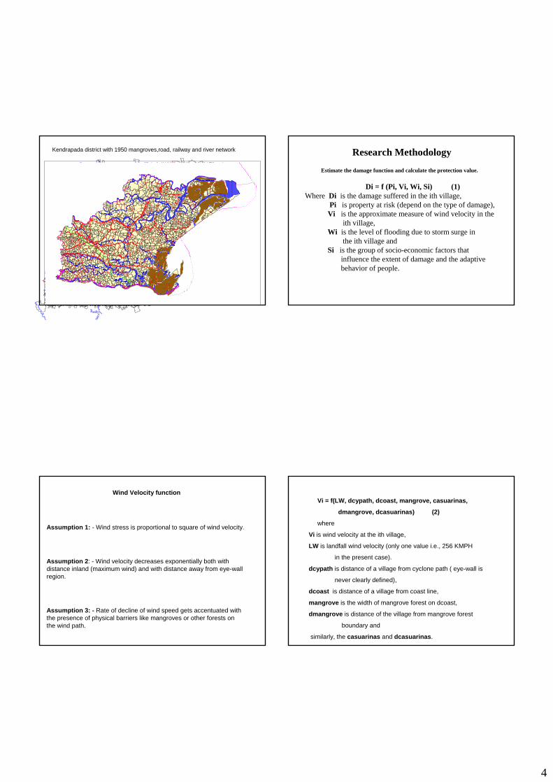
4

Kendrapada district with 1950 mangroves,road, railway and river network

Di = f (Pi, Vi, Wi, Si) (1)Where Di is the damage suffered in the ith village,

Pi is property at risk (depend on the type of damage),Vi is the approximate measure of wind velocity in the

ith village,Wi is the level of flooding due to storm surge in

the ith village andSi is the group of socio-economic factors that

influence the extent of damage and the adaptivebehavior of people.

Estimate the damage function and calculate the protection value.

Research Methodology

Wind Velocity function

Assumption 1: - Wind stress is proportional to square of wind velocity.

Assumption 2: - Wind velocity decreases exponentially both with distance inland (maximum wind) and with distance away from eye-wall region.

Assumption 3: - Rate of decline of wind speed gets accentuated with the presence of physical barriers like mangroves or other forests on the wind path.

Vi = f(LW, dcypath, dcoast, mangrove, casuarinas,

dmangrove, dcasuarinas) (2)

where

Vi is wind velocity at the ith village,

LW is landfall wind velocity (only one value i.e., 256 KMPH

in the present case).

dcypath is distance of a village from cyclone path ( eye-wall is

never clearly defined),

dcoast is distance of a village from coast line,

mangrove is the width of mangrove forest on dcoast,

dmangrove is distance of the village from mangrove forest

boundary and

similarly, the casuarinas and dcasuarinas.

5

Storm Surge Velocity function

Assumption 1: - Surge Velocity at any Village will depend on the level of Sea Elevation (height of water) at the coastal point lying at a minimum distance from the village.

Assumption 2: - Level of flooding and velocity of surge water goes down exponentially with distance inland and presence of barriers at the coast.

Assumption 3: -Sea Elevation at different places on the coast doesn’t depend only on the wind velocity at those places, but also on other factors like:

contd……

Contd…

(1) The direction of the place vis-à-vis the landfall,

(2) The bathymetry of the place,

(3) The radius of the maximum wind,

(4) The angle that cyclone path forms with the coast line,

(5) Pressure drop

(6) Speed of cyclone,

(7) Density of sea water,

(8) Period of astronomical tide etc. Assumption 4: -Simulated Surge envelop provided by the meteorologists

after taking into account the above mentioned factors is a near approximate measure of the sea elevation.

6

Wi = w(surge, dcoast, mangrove, casuarinas,

dmangrove, dcasuarinas, elevation, dmajriver,

dminriver) (3)

Where, Wi is the velocity of water (that is proportional to level of flooding) in a village due to surge,

surge is the level of sea elevation (in meter)at the coast facing the village,

elevation is the height of the village compared to sea,

dmajriver is the distance of the village from a major river,

dminriver is the distance from a minor river and others have already been explained.

Socio Economic Factors

Si = s(pop99, literate, schedulecaste, worker, nonworker, droad, roadumy) (4)pop99 is total population of a place in 1999, literate is the percentage of literate people( proxy for adaptive behavior to cyclone warning), schedulecaste is the percentage of scheduled caste and scheduledtribes in total population (economically most backward),

worker is the percentage of workers(earning members) in total population,nonworker is the percentage of dependants (not exposed to cyclone) in total population,

droad is minimum distance of the village from state highway(better scope to prosper) and

roadumy is a dummy variable for the presence of village road (easy connection to metal road).

Estimating Equation (putting eq2, 3 and 4 in eq1)

Di = f (LW, dcoast, dcypath, mangrove, casuarinas, dmangrove, dcasuarinas, surge, elevation, dmajriver, dminriver, tpop, literate, schedulecaste, worker, nonworker, droad, roadumy ) (5)where Di is the damage suffered in the ith village (no of human casualties, no of houses damaged or no of different types of livestock lost) and the explanatory variables have already been explained.

Non-linear regression estimates (tobit, poisson and nonlinear least squares) will be used to estimate the damage equation in accordance with the meteorological and fluid dynamics hypothesis.

Data Sources

. Emergency offices and Tahasildar offices of the Government of Orissa(Different types of damages).

• Digitized village map,coastal forest map,road network and river network map and GIS ARCVIEW software (different distances and width of forest) .

•P.W.D. dept, Govt of Orissa(elevation of villages; could get only 44 observations for 900 villages. Hence replaced elevation by topography dummy).

•Meteorology Dept of Govt of India (surge or the surge envelop).

7

Human Casualties Equation

sucydeathi = f( LW, dcoast, dcypath, mangrove, casuarinas, dmangrove, dcasuarinas, surge, elevation,dmajriver, dminriver,pop99, literate, schedulecaste, worker, nonworker, droad, roadumy)

sucydeathi is no of human death in a village during cyclone.

Variables dropped: - LW (one observation), casuarinas and dcasuarinas (very limited presence), dmangrove (captured same effect as dcoast) elevation (few observations).

Additional variables included: -

topodumy (based on 1950 mangrove and present mangrove to capture vulnerability; = 1if has mangrove today or in 1950, = 0 otherwise). block dummies ( efficiency of local administration) and percentage of different categories of workers

This equation has been estimated over four different areas to see the robustness of the results.

Area A: - Mahakalpada and Rajnagar block of Kendrapada (428 villages).

Area B: - Mahakalpada and Rajnagar blocks without the 32 villages that were habitated in between 1991 and 2001 census (396 villages).

Area C: - Makakalpada and Rajnagar blocks of Kendrapada and coastal villages of Chandbali block of Bhadrakh district (these villages are immediately after the mangrove forest) (513 villages).

Area D: - Mahakalpada, Rajnagar, Rajkanika, Aul and Patamundai blocks of Kendrapada district and Chandbali block of Bhadrakh district (898 villages).

0.800.530.72428nonworker

100.070.04428Otworker

0.07800.0070.002428Hhworker

100.090.26428Worker

100.170.12428Schedulecaste

100.130.56428Literate

60.982767.28745.28428Pop99

100.490.60428Roadumy

18.170.12.753.61428Droad

11.820.082.212.63428Dminriver

9.210.051.771.9428dmajriver

1002.141428mangrove

22.490.35.689.37428Dcoast

4.70.71.281.544284.7Surge

72.827.417.7140.58428dcypath

100.500.49428Topodummy

100.490.41428B5

100.490.58428B4

2101.780.54428Sucydeath

maxminStd.devmeanobsvariables

Summary statistics- Area A (death-234)

0.800.230.73396nonworker

100.070.04396Otworker

0.07800.0070.002396Hhworker

100.980.26396Worker

100.150.11396Schedulecaste

100.120.56396Literate

60.986780.36778.18396Pop99

100.490.60396Roadumy

13.550.12.543.46396Droad

11.820.082.172.59396Dminriver

9.210.051.771.9396dmajriver

1002.040.93396mangrove

22.490.345.719.57396Dcoast

4.70.71.261.593964.7Surge

72.827.417.6439.58396dcypath

100.500.48396Topodummy

100.490.44396B5

100.490.55396B4

2101.770.57396Sucydeath

maxminStd.devmeanobsvariables

Summary statistics- Area B (death =234)

8

Variable| Obs Mean Std. Dev. Min Max

sucydeath 513 .48 1.62 0 21

b4 513 .48 .50 0 1

b5 513 .34 .47 0 1

b6 513 .16 .37 0 1

topodumy 513 .41 .49 0 1

dcypath 513 45.46 19.71 7.4 83

surge1 513 1.38 1.18 .6 4.7

dcoast 513 10.09 6.1 .3 30.67

mangrove 513 1.24 2.61 0 10

dmajriver 513 2.47 2.76 .05 26.48

dminriver 513 3.22 3.04 .08 19.1

droad 513 3.76 2.79 .06 18.17

roadumy 513 .62 .48 0 1

pop99 513 746.23 739.28 2 6098

literate 513 .56 .14 0 1.85

scheduleca~e 513 .13 .19 0 1.08

worker 513 .26 .11 0 1.34

hhworker 513 .002 .007 0 .07

otworker 513 .04 .06 0 1.2

nonworker 513 .72 1.00 0 0.8

Summry statistics Area C ( death=244)

0.800.720.72897nonworker

100.050.05897Otworker

0.07800.0070.003897Hhworker

100.090.24897Worker

100.190.16897Schedulecaste

100.130.60897Literate

60982789.98851.3897Pop99

100.470.68897Roadumy

18.170.063.363.66897Droad

19.10.012.612.82897Dminriver

6.80.054.253.28897Dmajriver

1002.361.29897Mangrove

38.740.38.815.1897Dcoast

4.70.60.9281.26897Surge

837.416.643.67897Dcypath

100.4260.237897Topodumy

100.3080.106897B6

100.390.198897B5

100.450.279897B4

100.360.158897B3

100.340.132897B2

100.330.129897B1

2101.260.315897Sucydeath

minmaxStd.devmeanobsvariables

Summary Statistics – Area D (death=284)

-0.84 (-1.15)-0.22 (-0.31)-0.68 (-0.95)-1.08 (-1.46)constant

-0.46** (-1.95)-0.57** (-2.2)--------------Nonworker

-3.60** (-2.16)-3.02* (-1.87)---------------Otworker

26.99*** (2.82)24.99*** (2.71)---------------Hhworker

--------------0.233 (-0.25)-0.64 (-0.67)Worker

-2.00*** (-3.17)-2.14*** (-3.37)-1.84*** (-3.08)-1.76*** (-2.98)Schedulecaste

-0.96 (-1.44)-1.18* (-1.78)-1.18* (-1.79)-0.95 (-1.41)Literate

0.0005***(10.6)0.0006*** (10.9)0.0005***(11.5)0.0005*** (10.8)Pop99

-0.159 (-1.01)-0.117 (-0.76)-0.144 (-0.92)-0.194 (-1.22)Roadumy

-0.016 (-0.52)0.011 (0.37)0.02 (0.66)-0.008 (-0.26)Droad

-0.122** (-2.32)-0.13** (-2.48)-0.111** (-2.1)-0.1.8** (-2.03)Dminriver

0.0001 (00)-0.024 (-0.50)-0.017 (-0.36)0.007 (0.15)Dmajriver

-0.84*** (-5.12)-0.79*** (-5.12)-0.745*** (-5.0)-0.81*** (-5.02)Mangrove

0.028 (1.24)0.021 (0.92)0.028 (1.23)0.034(1.5)Dcoast

0.12* (1.83)0.119** (1.86)0.116* (1.76)0.12*(1.81)Surge

0.027** (2.15)-0.3 (-0.31)-0.003 (-0.33)0.03**(2.15)Dcypath

0.77*** (3.43)1.01***(4.82)0.97*** (4.61)0.71***(3.14)Topodumy

-----------------------------B5

-1.16*** (-2.99)----------------1.18*** (-3.06)B4

Equation 4Equation 3Equation 2Equation 1Inde. Variable

Poisson Results- Area A: Dependant Variable = sucydeath, 428 villages

*** is significant at 1%, ** is significant at 5 % and * is significant at 10 %. Bracketed figures are the z values.

-0.24 (-0.33)0.19 (0.27)-0.21 (-0.27)-0.37 (-0.47)constant

-0.48** (-2.04)-0.57** (-2.23)-----------Nonworker

-3.43** (-2.07)-2.79* (-1.76)-----------Otworker

25.01*** (2.65)23.54** (2.57)------------Hhworker

---------------0.63 (-0.56)-1.29 (-1.6)Worker

-1.67*** (-2.7)-1.83*** (-2.98)-1.54*** (-2.62)-1.43** (-2.44)Schedulecaste

-1.21* (-1.69)-1.53** (-2.18)-1.52** (-2.23)-1.22* (-1.74)Literate

0.0005*** (9.8)0.0005*** (10.1)0.0005*** (10.5)0.0005*** (9.9)Pop99

-0.25 * (-1.6)-0.235 (-1.48)-0.25 (-1.58)-0.287* (-1.77)Roadumy

-0.39 (1.10)-0.003 (-0.11)0.005 (0.14)-0.034 (-0.48)Droad

-0.088* (-1.65)-0.102 ** (-1.92)-0.083 (-1.53)-0.07 (-1.28)Dminriver

0.024 (0.49)-0.002 (-0.04)0.007 (0.14)0.33 (0.68)dmajriver

-1.24*** (-5.65)-1.13*** (-5.69)-1.07*** (-5.54)-1.201*** (-5.55)Mangrove

0.016 (0.68)0.015 (0.63)0.23 (0.97)0.023 (0.97)Dcoast

0.106* (1.57)0.111 (1.64)0.104 (1.56)0.098 (1.47)Surge

0.018 (1.37)-0.007 (-0.87)-0.007 (-0.84)0.018 (1.47)Dcypath

0.99*** (3.98)1.26*** (5.56)1.23*** (5.45)0.96*** (3.89)Topodumy

---------------------B5

-1.09*** (-2.58)------------1.14*** (-2.70)B4

Equation 4Equation 3 Equation 2Equation 1Inde.variable

Poisson Results – Area B ; Dependant Variable = sucydeath, 396 villages

*** is significant at 1 %, ** is significant at 5 % and * is significant at 10 %. Bracfketed values are the z values.

9

-1.98* (-1.68)-0.59 (-0.97)-0.99 (-1.56)-2.45* (-2.07)constant

-0.47** (-2.01)-0.55** (2.16)----------Nonworker

-2.07 (-1.24)-1.72 (-1.19)--------Otworker

24.36*** (2.62)21.35** (2.38)--------Hhworker

----------0.103 (-0.12)-0.56 (-0.59)Worker

-1.67*** (-2.99)-1.71*** (-3.08)-1.46*** (-2.78)-1.41** (2.67)Sche.caste

-1.15* (-1.82)-1.34** (-2.11)-1.31** (-2.12)-1.08* (-1.72)Literate

0.0005*** (10.3)0.0005*** (10.9)0.0005*** (11.8)0.0005***(10.9)Pop99

-0.15 (-0.99)-0.103 (-0.68)-0.123 (-0.82)-0.176 (-1.15)Roadumy

-0.02 (-0.56)0.007 (0.26)0.015 (0.52)-0.01 (-0.30)Droad

-0.111*** (-2.65)-0.107** (-2.50)-0.096** (-2.24)-0.102** (-2.41)Dminriver

0.028 (0.85)0.027 (0.85)0.027 (0.86)0.033 (0.99)Dmajriver

-0.66*** (-4.67)-0.639*** (-4.4)-0.619*** (-4.85)-0.645*** (-4.68)Mangrove

0.03 (1.44)0.033* (1.68)0.035* (1.83)0.034 (1.6)Dcoast

0.132** (2.03)0.138** (2.13)0.132** (2.05)0.129** (2.01)Surge

0.23* (1.88)0.0005 (0.08)-0.0002 (-0.03)0.024** (1.99)Dcypath

0.78*** (3.49)0.99*** (4.82)0.97*** (4.73)0.74*** (3.31)Topodumy

---------------------B5

1.14 (1.58)----------1.30* (1.85)B5

0.08 (0.18)-----------0.21 (0.44)B4

Equation4Equation 3Equation 2Equation 1Depe.variable

Poisson Results –Area C; Dependant variable = sucydeath, 513 villages.

-1.72 (-1.54)0.19 (0.36)-0.34 (-0.61)-2.12** (-1.99)constant

-0.45** (-1.94)-0.62** (-2.3)-------Nonworker

-1.81 (-1.25)-2.54* (-1.75)--------Otworker

20.46** (2.26)18.87** (2.15)---------Hhworker

---------0.48 (0.64)-0.47 (-0.54)Worker

-1.22** (-2.56)-1.42*** (-2.95)-1.3*** (-2.83)-1.03** (2.24)Sche.caste

-0.98* (-1.61)-1.80*** (-3.05)-1.91*** (-3.3)-0.91 (-1.5)Literare

0.0005*** (11.0)0.0005*** (11.4)0.0005*** (12.15)0.0005*** (11.4)Pop99

-0.166 (-1.17)-0.153 (-1.09)-0.16 (-1.13)-0.18 (-1.29)Roadumy

-0.034 (-1.33)-0.02 (-0.98)-0.017 (-0.76)-0.03 (-1.18)Droad

-0.098*** (-2.53)-0.077** (-1.97)-0.064* (-1.65)-0.089** (-2.29)Dminriver

0.034 (1.44)0.034** (1.97)0.03** (1.92)0.036 (1.53)Dmajriver

-0.639*** (4.62)-0.723*** (-5.69)-0.684*** (-5.5)-0.626*** (-4.57)Mangrove

0.013 (0.86)-0.014 (-1.11)-0.013 (-1.04)0.014 (0.91)Dcoast

0.133*** (2.08)0.22*** (3.63)0.222*** (3.68)0.13** (2.07)Surge

0.019 (1.59)-0.005 (-0.94)-0.006 (-1.07)0.019* (1.68)Dcypath

0.75*** (3.6)1.09*** (5.72)1.03*** (5.41)0.70*** (3.42)Topodumy

---------------------B6

1.13* (1.69)---------1.27* (1.88)B5

0.09 (0.2)----------0.18 (0.41)B4

-15.38 (-0.02)-----------15.9 (-0.01)B3

-0.06 (-0.12)-----------0.05 (-0.09)B2

-0.83 (-1.56)--------------0.84 (-1.59)B1

Equation 4Equation 3Equation 2Equation 1Inde. variable

Poisson Result – Area D; Dependant variable = sucydeath, 897 villages

Prediction based on Equation 3 of Area D results.

Predicted human death without and with the mangrove forest = 387-283 = 104

Combined marginal effect of topography dummy and mangrove vegetation = 0.1154.

Conclusion: -

1. Mangrove forest seems to have played a strong protective role in averting human death during the super cyclone of Oct. 1999.

2. The result is robust and independent of the sample size.

3. Without the forest, it seems, another 104 persons would have died in area D or in those 897 villages.

4. The combined effect of topography dummy and mangrove vegetation being positive, it seems, even if we grow mangrove in all low lying vulnerable areas where mangrove existed historically, human casualties can’t be averted 100 %. Few casualties will still occur. But there could be substantial reduction in death.

GRAM PANCHYATS– PURI (Casuarinas areas)

10

0.54690.17390.13550.3159391worker100.23320.2189391Sche.caste

0.8300.29630.6687391Literate

727011860.3337820.4629391Pop-1999

10.650.062.09352.4634391Droad

2.200.45290.1339391Native forest

2.800.95390.9904391Casuarinas

45254.108433.8929391Dcypath

180.374.35248.7009391Dcoast

1001.18490.4808391sucydeath

maxminStd.devmeanobsvariables

Summary Statistics- Casuarinas areas (Death=188, only wind)

0.0003.845.62582_cons |

0.857-0.18-.2593642marworker

0.4580.74.0646499Nonworker

0.7880.27.4702554Worker

0.3840.87.3295678Sche.caste

0.0222.292.972111Literate

0.0007.79.0003825pop_1999

0.9320.09.0054494Driver

0.4000.84.0426315Droad

0.171-1.37-.3028221Native forest

0.095-1.67-.1773471Casuarinas

0.000-6.92-.2214735Dcypath

0.000-5.44-.1489863Dcoast

0.013-2.49-.4774582rddmy

P>|z|zCoefInde.var

Poisson Result (casuarinas areas), Dept.var = sucydeath

Forest type Obs Mean Std. Dev. Min Max

Casuarinas 391 -.085 .142 -1.687 -.0061

Native forest 391 -.146 .243 -2.881 -.0105

Mangroves 427 -.615 1.208 -11.414 -1.26e-0

Comparison of Marginal effect

Conclusion•Casuarinas forest, the shelterbelt plantation of government, have low protective capacity for human life compared to other forests.

•Mixed indigenous forests seems to be having better protective capacity than casuarinas.

11

-1.72 (-1.54)0.19 (0.36)-0.34 (-0.61)-2.12** (-1.99)constant

-0.45** (-1.94)-0.62** (-2.3)-------Nonworker

-1.81 (-1.25)-2.54* (-1.75)--------Otworker

20.46** (2.26)18.87** (2.15)---------Hhworker

---------0.48 (0.64)-0.47 (-0.54)Worker

-1.22** (-2.56)-1.42*** (-2.95)-1.3*** (-2.83)-1.03** (2.24)Sche.caste

-0.98* (-1.61)-1.80*** (-3.05)-1.91*** (-3.3)-0.91 (-1.5)Literare

0.0005*** (11.0)0.0005*** (11.4)0.0005*** (12.15)0.0005*** (11.4)Pop99

-0.166 (-1.17)-0.153 (-1.09)-0.16 (-1.13)-0.18 (-1.29)Roadumy

-0.034 (-1.33)-0.02 (-0.98)-0.017 (-0.76)-0.03 (-1.18)Droad

-0.098*** (-2.53)-0.077** (-1.97)-0.064* (-1.65)-0.089** (-2.29)Dminriver

0.034 (1.44)0.034** (1.97)0.03** (1.92)0.036 (1.53)Dmajriver

-0.639*** (4.62)-0.723*** (-5.69)-0.684*** (-5.5)-0.626*** (-4.57)Mangrove

0.013 (0.86)-0.014 (-1.11)-0.013 (-1.04)0.014 (0.91)Dcoast

0.133*** (2.08)0.22*** (3.63)0.222*** (3.68)0.13** (2.07)Surge

0.019 (1.59)-0.005 (-0.94)-0.006 (-1.07)0.019* (1.68)Dcypath

0.75*** (3.6)1.09*** (5.72)1.03*** (5.41)0.70*** (3.42)Topodumy

---------------------B6

1.13* (1.69)---------1.27* (1.88)B5

0.09 (0.2)----------0.18 (0.41)B4

-15.38 (-0.02)-----------15.9 (-0.01)B3

-0.06 (-0.12)-----------0.05 (-0.09)B2

-0.83 (-1.56)--------------0.84 (-1.59)B1

Equation 4Equation 3Equation 2Equation 1Inde. variable

Poisson Result – Area D; Dependant variable = sucydeath, 897 villages

-1.62 (-1.39)0.72 (1.29)0.25 (0.43)-1.93* (-1.70)constant

-0.46 ** (-2.07)-0.66** (-2.45)-------Nonworker

-1.18 (-0.85)-1.52 (-1.13)--------Otworker

18.88 ** (2.04)17.6** (1.98)---------Hhworker

----------0.01 (-0.01)-1.57 (-1.47)Worker

-0.61 (-1.34)-0.90** (-1.97)-0.75 * (-1.72)-0.36 (-0.83)Sche.caste

-1.08 * (-1.74)-2.06*** (-3.39)-2.06*** (-3.48)-0.86 (-1.35)Literare

0.0004*** (9.9)0.0004*** (10.36)0.0004*** (11.2)0.0004*** (10.75)Pop99

-0.16 (-1.14)-0.129 (-0.91)-0.15 (-1.03)-0.21 (-1.45)Roadumy

-0.06 ** (-2.33)-0.031 (-1.30)-0.02 (-1.02)-0.06** (-2.28)Droad

-0.11*** (-2.77)-0.09** (-2.37)-0.08** (-2.09)-0.102** (2.57)Dminriver

0.06 ** (2.53)0.051** (2.49)0.051** (2.43) 0.069 *** (2.82)Dmajriver

-1.28*** (-5.40)-1.02*** (-4.57)-0.96*** (-4.36)-1.31*** (-5.49)mi

-0.004 (-0.29) * -0.025(-1.87)-0.03** (-1.97)-0.007 (-0.46)Dcoast

0.08 (1.31)0.197*** (3.21)0.20*** (3.28)0.081 (1.25)Surge

0.02* (1.71)0.0009 (-1.5)-0.01 (1.56)0.02** (1.95)Dcypath

0.60*** (2.80)1.03*** (5.35)0.99*** (5.21)0.56*** (2.66)Topodumy

---------------------B6

1.68** (2.30)---------1.97*** (2.72)B5

0.19 (0.41)----------0.325 (0.64)B4

-10.91 (-0.02)-----------11.26 (-0.02)B3

0.23 (0.40)----------0.29 (0.52)B2

-0.47 (-0.85)--------------0.42 (-0.74)B1

Equation 4Equation 3Equation 2Equation 1Inde. variable

Poisson Result – Area D; mi ≤ 1.5 km; No of villages = 626.

-1.83 (-1.59)0.12 (0.20)0.32 (0.49)-1.58 (-1.33)constant

-0.19 (-0.67)-0.29 (-0.86)-------Nonworker

-1.01 (-0.75)-1.96 (-1.37)--------Otworker

17.5 ** (2.0)16.37 * (1.87)---------Hhworker

-------------0.31 (-0.37)-2.02 ** (-1.89)Worker

-0.40 (-0.86)-0.59 (-1.20)-0.60 (-1.27)-0.19 (-0.42)Sche.caste

-0.57 (-0.87)-1.48 ** (-2.27)-1.8 *** (-2.83)-0.38 (-0.55))Literare

0.0005 *** (10.2)0.0005 *** (10.4)0.0005*** (10.9)0.0005*** (10.7)Pop99

-0.17 (-1.1)-0.12 (-0.79)-0.17 (-1.15)-0.22 (-1.44)Roadumy

-0.06 ** (-2.13)-0.02 (-0.85)-0.02 (-0.72)-0.07 ** (2.24)Droad

-0.09 ** (-2.29)-0.09 ** (-2.12)-0.07 * (-1.79)-0.09 ** (-2.20)Dminriver

0.05 * (1.79)0.04 * (1.83)0.04 * (1.61)0.05 **(2.03)Dmajriver

-0.68 *(-1.83)-0.83 ** (-2.23)-0.65 ** (-1.76)-0.72 ** (-1.96)Mi

-0.008 (-0.43)-0.03 ** (-2.56)-0.03 ** (-2.39)-0.01 (-0.66)Dcoast

0.04 (0.65)0.20 *** (3.22)0.18 *** (2.87)0.03 (.40)Surge

0.017 (1.43)-0.01 * (-1.84)-0.01 * (-1.74)0.02 (1.50)Dcypath

0.56 ** (2.54)0.86 *** (4.26)0.93* ** (4.62)0.54 ** (2.47)Topodumy

---------------------B6

1.55 ** (2.08)---------1.78 ** (2.41)B5

0.03 (0.07)----------0.09 (0.18)B4

-----------------------B3

-0.05 (-0.09)-----------0.07 (-0.14)B2

-0.69 (-1.25)--------------0.71 (-1.32)B1

Equation 4Equation 3Equation 2Equation 1Inde. variable

Poisson Result – Area D; Mi ≤ 0.8 (0 to 0.76); 567 villages