Embed Size (px)
Citation preview

1
Ph.D. in Electronic and Computer Engineering
Dept. of Electrical and Electronic Engineering
University of Cagliari
Title: Wavelet Spectrum Sensing and Transmission
System (WS-SaT-System) based on WPDM
Author: Valeria Orani
Advisor: Daniele Giusto
Curriculum: ING-INF/ 03 (Telecomunicazioni)
Dottorato in Ingegneria Elettronica e Informatica
Dipartimento di Ingegneria Elettrica ed Elettronica
Università degli Studi di Cagliari
Titolo: Wavelet Spectrum Sensing and Transmission
System based on WPDM (WS-SaT-System)
Autore: Valeria Orani
Tutor: Daniele Giusto
Settore: ING-INF/03 (Telecomunicazioni)
XXI Ciclo

2
Table of Contents
List of Figures.................................................................... 5
Introduction....................................................................... 8
Chapter I.......................................................................... 15
State of the art of spectrum sensing techniques for
dynamical and distributed radio access ........................ 15
1. Signal processing techniques for spectrum sensing ...............................................................16
1.1 Matched Filter ..........................................................................................................................16
1.2 Energy Detector........................................................................................................................17
1.2.1 Parallel MRSS Sensing ....................................................................................................18
1.2.2 MRSS Sensing with wavelet generators ..........................................................................20
1.3 Cyclostationary Feature Detector............................................................................................22
1.4 Mixed mode sensing schemes ..................................................................................................25
1.5 Cooperative Spectrum Sensing ................................................................................................26
1.6 Cooperative techniques ............................................................................................................27
1.6.1 Decentralized Uncoordinated Techniques .......................................................................27
1.6.2 Centralized Coordinated Techniques ...............................................................................27
1.6.3 Decentralized Coordinated Techniques ...........................................................................28
1.7 Benefits of cooperation ............................................................................................................29
1.8 Disadvantages of cooperation..................................................................................................30
1.9 Sensor networks for spectrum sensing ....................................................................................32
1.10 Design of a Spectrum Sensing System using the DWPT transformation............................33
Chapter II ........................................................................ 34
State of the art on cognitive radio transmission ........... 34
2.1 Modulation formats..................................................................................................................36
2.1.1 OFDM ..............................................................................................................................36
2.1.2 Adaptive modulation........................................................................................................38

3
2.2 Power Scaling...........................................................................................................................41
2.3 Radio design architectures.......................................................................................................44
2.3.1 Antenna issues..................................................................................................................44
2.3.2 Multi-transmission methods.............................................................................................47
2.3.3 High performance, multi – band implementation ............................................................48
2.4 Design of a transmission system using the WPDM ................................................................51
2.4.1 Theoretical background....................................................................................................51
Chapter III....................................................................... 55
Wavelet Filter Bank........................................................ 55
3.1 Introduction..............................................................................................................................55
3.2 Continuous wavelet transform.................................................................................................56
3.3 Discrete wavelet transform ......................................................................................................58
Chapter IV....................................................................... 64
Design of a spectrum sensing system using the Discrete
Wavelet Packet Transformation (DWPT) and WPDM
transmission system ........................................................ 64
4.1 Wavelet multiresolution analysis and DWPT .........................................................................64
4.2 Spectrum Sensing Algorithms .................................................................................................68
4.2.1 Power Analysis ................................................................................................................68
4.2.2 Histograms Analysis ........................................................................................................69
4.2.3 Simulation results.............................................................................................................71
4.3 Transmitting and receiving data..............................................................................................76
4.3.1 System Architecture.........................................................................................................76
4.3.2 Simulation results and performance tests.........................................................................78
BER – without channel equalization.........................................................................................78
Sampling phase offset ...............................................................................................................79
Presence of a narrow band interferer ........................................................................................81
4.4 Possible schemes of simulation and different configuration of the system ...........................84
4.4.1 Communication based on a Coordinator..........................................................................84
4.4.2 Communication without a Coordinator............................................................................85

4
4.5 Simulink transmission model ..................................................................................................88
Chapter V ........................................................................ 97
A case of study: “A cognitive radio system for home
theatre 5+1 audio surround applications” .................... 97
5.1 AC-3 ..........................................................................................................................................97
5.1.1 Encoding .......................................................................................................................100
5.1.2 Decoding ........................................................................................................................101
5.2 Communication architecture .................................................................................................103
Conclusions.................................................................... 104
Bibliography .................................................................. 106
REFERENCES............................................................................................................................106

5
List of Figures
Figure 1. Spectrum usage measurements averaged over six locations.
Figure 2. A generic architecture of a cognitive radio transceiver.
Figure 3. Traditional radio, software radio, and cognitive radio.
Figure 4. Block diagram of a matched filter detector.
Figure 5. Parallel, multi-resolution system configured for the coarse resolution, and fine resolution
sensing modes.
Figure 6. MRSS with analog wideband spectrum sensing.
Figure 7. Block diagram of a cyclostationary feature detector.
Figure 8. Combined decision scheme based on wideband energy detection with feature detection
for a single channel.
Figure 9. Cooperation Techniques among CR. Decentralized coordination technique and
centralized coordinated techniques as partial or total cooperative.
Figure 10. Schematic of an NC – OFDM transceiver.
Figure 11. Basic block diagram of an adaptive modulation - based cognitive radio system.
Figure 12. Network configuration for a method for robust transmission power and position
estimation in cognitive radio.
Figure 13. Typical hardware architecture of a cognitive radio.
Figure 14. Radio architectures with parallel (a) and combined sensing and communication (b).
Figure 15. Multi – transmission architecture.
Figure 16. Architecture of the cognitive radio platform.
Figure 17. Baseband processor architecture – block structure.
Figure 18. Wavelet packet elementary block decomposition and reconstruction.
Figure 19. The steps of an easy recipe for creating a CWT.
Figure 20. Wavelet filter bank.

6
Figure 21. Uniform wavelet packet decomposition.
Figure 22. Asymmetric wavelet packet decomposition.
Figure 23. Wavelet families (a) Haar (b) Daubechies4 (c) Coiflet1 (d) Symlet2 (e) Meyer (f) Morlet
(g) Mexican Hat.
Figure 24. Transmitter and receiver for two level WPDM system.
Figure 25. (a) Wavelet tree structure (b) Corresponding symbolic subband structure.
Figure 26. Spectrum sensing algorithm based on power estimation.
Figure 27. Spectrum sensing algorithm based on histogram analysis.
Figure 28. Spectrum of a generic signal.
Figure 29. Separation of the input bandwidth in 16 sub bands using 4-level DWPT
Figure 30. Sub-channel 15: a histogram of a free subband
Figure 31. Sub-channel 3: a histogram of an occupied subband
Figure 32. A generic signal at a CPE.
Figure 33. Sub-channel 6: a histogram of a free subband.
Figure 34. Sub-channel 3: a histogram of an occupied subband.
Figure 35. Architecture of the transmission system using WPM technology.
Figure 36. Architecture of the receiver using WPM technology.
Figure 37. Performance of WPM versus OFDM in a 2-path time-invariant channel. BER is plotted
as a function of the delay of arrival of the second path. The delayed path relative power of −3 dBc
and the SNR is 20 dB.
Figure 38. Sensitivity of different WPM schemes versus OFDM schemes to sampling phase error,
expressed as the link BER versus the normalized sampling phase error.
Figure 39. Link BER in the presence of a single tone disturber as a function of the disturber
frequency, for WPM(coif1), WPM(coif5), WPM(dmey), and OFDM schemes.
Figure 40. Link BER in the presence of a single tone disturber as a function of the disturber power,
for WPM(coif1), WPM(coif5), WPM(dmey), and OFDM schemes.
7
Figure 41. Configuration based on a coordinator.
Figure 42. Spectrum sensing using WPDM with e.g. 5 levels.
Figure 43. Communication sequence between two secondary users: Step 1
Figure 44. Communication sequence between two secondary users: Step 2
Figure 45. Communication sequence between two secondary users: Step 3
Figure 46. Example application of AC-3 to satellite audio transmission.
Figure 47. The AC-3 encoder.
Figure 48. The AC-3 decoder.
Figure 49. System configuration with a coordinator.

8
Introduction
Today’s wireless networks are characterized by fixed spectrum assignment policy. With ever
increasing demand for frequency spectrum and limited resource availability FCC decided to make a
paradigm shift by allowing more and more number of unlicensed users to transmit their signals in
licensed bands so as to efficiently utilize the available spectrum. The motivating factor behind this
decision was the findings in a report by Spectrum Policy Task Force, in which vast temporal and
geographic variations in spectrum usage were found ranging from 15% to 85%. Most of the allotted
channels are not in use most of the time; some are partially occupied while others are heavily used.
Figure 1 shows spectrum utilization in the frequency bands between 30 MHz and 3 GHz averaged
over six different locations. The relatively low utilization of the licensed spectrum suggests that
spectrum scarcity, as perceived today, is largely due to inefficient fixed frequency allocations rather
than any physical shortage of spectrum.
In May 2004, FCC released a report [1] in which it took an initiative which allows the use of this
underutilized spectrum to unlicensed users (users that are not been served by the primary license
holders) to operate in television spectrum in areas where the spectrum is not in use. However, these
unlicensed users should not create interference to the licensed user and at times the licensed user
wants to transmit its signal while the unlicensed user should vacate the spectrum and should look
for some other free space.
At the present time there is much research and investigation by many industrial organizations and
national administrations on the closely related topics of dynamic spectrum management, flexible
spectrum management, advanced spectrum management, dynamic spectrum allocation, flexible
spectrum use, dynamic channel assignment, and opportunistic spectrum management.
Cognitive radio (CR) and the closely related technologies of policy-based adaptive radio, software
defined radio, software controlled radio, and reconfigurable radio are enabling technologies to

9
implement these new spectrum management and usage paradigms. These concepts are equally
applicable to a wide variety of mobile communications systems including public protection and
disaster relief (PPDR), military, and commercial wireless networks.
Figure 1. Spectrum usage measurements averaged over six locations
There are many definitions of CR and definitions are still being developed both in academia and
through standards bodies, such as IEEE-1900 and the Software Defined Radio Forum.

10
The cognitive radio concept was first introduced by Mitola, in his PhD thesis, where he explains:
“the term cognitive radio identifies the point in which wireless personal digital assistants (PDAs)
and the related networks are sufficiently computationally intelligent about radio resources and
related computer-to-computer communications to detect user communications needs as a function
of use context, and to provide radio resources and wire less services most appropriate to those
needs”.
Cognitive radio refers to wireless architectures in which a communication system does not operate
in a fixed band, but rather searches and finds an appropriate band in which to operate.
This means that wherever the user goes, cognitive device will adapt to new environment allowing
user to be always connected.
Cognitive radio will lead to a revolution in wireless communication with significant impacts on
technology as well as regulation of spectrum usage to overcome existing barriers.
The term cognitive radio is derived from “cognition”.
According to Wikipedia cognition is referred to as
� Mental processes of an individual, with particular relation.
� Mental states such as beliefs, desires and intentions.
� Information processing involving learning and knowledge.
� Description of the emergent development of knowledge and concepts within a group.
Resulting from this definition, the cognitive radio is a self-aware communication system that
efficiently uses spectrum in an intelligent way. It autonomously coordinates the usage of spectrum
in identifying unused radio spectrum on the basis of observing spectrum usage. The classification of
spectrum as being unused and the way it is used involves regulation, as this spectrum might be
originally assigned to a licensed communication system. This secondary usage of spectrum is
referred to as vertical spectrum sharing. To enable transparency to the consumer, cognitive radios
provide besides cognition in radio resource management also cognition in services and applications.

11
Cognition is illustrated at the example of flexible radio spectrum usage and the consideration of
user preferences. In observing the environment, the cognitive radio decides about its action. An
initial switching on may lead to an immediate action, while usual operation implies a decision
making based on learning from observation history and the consideration of the actual state of the
environment.
The Federal Communications Commission (FCC) has identified in the following (less
revolutionary) features that cognitive radios can incorporate to enable a more efficient and flexible
usage of spectrum:
� Frequency Agility – The radio is able to change its operating frequency to optimize its use
in adapting to the environment.
� Dynamic Frequency Selection (DFS) – The radio senses signals from nearby transmitters
to choose an optimal operation environment.
� Adaptive Modulation – The transmission characteristics and waveforms can be
reconfigured to exploit all opportunities for the usage of spectrum
� Transmit Power Control (TPC) – The transmission power is adapted to full power limits
when necessary on the one hand and to lower levels on the other hand to allow greater
sharing of spectrum.
� Location Awareness – The radio is able to determine its location and the location of other
devices operating in the same spectrum to optimize transmission parameters for increasing
spectrum re-use.
� Negotiated Use – The cognitive radio may have algorithms enabling the sharing of
spectrum in terms of prearranged agreements between a licensee and a third party or on an
ad-hoc/real-time basis.
The limited available spectrum and the inefficiency in the spectrum usage require a new
communication method to exploit the existing wireless spectrum opportunistically. This new

12
networking method is called the cognitive radio network and is referred by Ian F. Akyildiz as the
NeXt Generation (xG) Networks as well as Dynamic Spectrum Access (DSA).
The cognitive radio enables the usage of temporally unused spectrum, which is referred to as
spectrum hole or white space. If the band is further used by a licensed user, the cognitive radio
moves to another spectrum hole or stays in the same band, altering its transmission power level or
modulation scheme to avoid interference
A generic architecture of a cognitive radio transceiver is shown in the following figure.
Radio
Frequency
(RF)
Analog-to-
Digital
Converter
(A/D)
Baseband
Processing
Figure 2. A generic architecture of a cognitive radio transceiver
The main components of a cognitive radio transceiver are the radio front-end and the baseband
processing unit. In this architecture, a wideband signal is received through the RF front-end,
sampled by the high speed analog-to-digital (A/D) converter, and measurements are performed for
the detection of the licensed user signal.
The components of the cognitive radio network architecture can be classified in two groups as the
primary network and the cognitive network. Primary network is referred to as the legacy network
that has an exclusive right to a certain spectrum band. On the contrary, cognitive network does not
have a license to operate in the desired band.

13
Figure 3. Traditional radio, software radio, and cognitive radio
Figure 3 graphically contrasts traditional radio, software radio, and cognitive radio.
This thesis develops a new wavelet approach using the Wavelet Packet Decomposition (WPD) for
sensing the spectrum and also for information transmission by unlicensed users in licensed bands;
the approach is justified by flexible properties of wavelets, which offer the possibility of taking into
account variable channel conditions by decomposing recursively the spectrum into different
subbands.
The information about the transmission opportunities offered by the spectrum could be exploited by
a secondary user without causing interference to the primary one. Once transmission parameters are
defined, the transmitter uses the wavelet modulation scheme to send information.
The thesis is structured as follows.
In chapter I and II an overview of the state of art of sensing and transmitting techniques is given.
Chapter III gives a brief overview of wavelet filter bank and the wavelet packet decomposition
(WPD).
RF Modulation Coding Framing Processing
RF Modulation Coding Framing Processing
RF Modulation Coding Framing Processing
Hardware
Hardware
Hardware
Software
Software
Software
Intelligence (Sense, Learn, Optimize)
Traditional
Radio
Software
Radio
Cognitive
Radio

14
In chapter IV, a new method to sense the spectrum and individuate possibilities for transmission by
unlicensed users, using a Wavelet Packet Decomposition Multiplexing (WPDM) system, is
presented. In chapter V, the AC-3 system is described and a scenario of application of our technique
is given as an example to highlight the possibilities of the proposed method.
All simulations are done in MATLAB.

15
Chapter I
State of the art of spectrum sensing techniques for
dynamical and distributed radio access
The increased demand for mobile communications and new wireless applications raises the need for
a new approach to efficiently use the available spectrum resources. The current static assignment of
spectrum to specific users by regulatory bodies, the actual demand for transmission resources often
exceeds the available bandwidth. Promising approaches to overcome static spectrum assignments
are given by dynamic spectrum sharing systems. Important examples of these technologies are
overlay systems in which the spectral resources left idle by the primary (licensed) users are offered
to secondary users. Obviously, the terminals in the secondary systems must be able to detect an
emerging primary user immediately as well as reliably. These types of terminals are known as
Cognitive Radios (CR), which can be defined as self-learning, adaptive and intelligent radios with
the capacity to sense the radio environment and to adapt to the current conditions like available
frequencies and channel properties [13]. The spectrum sensing capacities of the CR rely on
advanced signal processing techniques, detailed in the following paragraphs.

16
1. Signal processing techniques for spectrum sensing
1.1 Matched Filter
The optimal way for any signal detection is a matched filter, since it maximizes received signal-to-
noise ratio. However, a matched filter effectively requires demodulation of a primary user signal.
This means that cognitive radio has a priori knowledge of primary user signal at both PHY and
MAC layers, e.g. modulation type and order, pulse shaping, packet format. Such information might
be pre-stored in CR memory, but the cumbersome part is that for demodulation it has to achieve
coherency with primary user signal by performing timing and carrier synchronization, even channel
equalization. This is still possible since most primary users have pilots, preambles, synchronization
words or spreading codes that can be used for coherent detection. For example: TV signal has
narrowband pilot for audio and video carriers; CDMA systems have dedicated spreading codes for
pilot and synchronization channels; OFDM packets have preambles for packet acquisition and so on
[1].
If X[n] is completely known to the receiver then the optimal detector for this case is
γ1
0
1
0
][][)( H
H
N
n
nXnYYT ∑−
=
<>= (I.1)
If γ is the detection threshold, then the number of samples required for optimal detection is
11211 )()()](([ −−−− =−= SNROSNRPQPQN FDD (I.2)
where PD and PFD are the probabilities of detection and false detection respectively [2].

17
Hence, the main advantage of matched filter is that due to coherency it requires less time to achieve
high processing gain since only O(SNR)-1
samples are needed to meet a given probability of
detection constraint. However, a significant drawback of a matched filter is that a cognitive radio
would need a dedicated receiver for every primary user class.
1.2 Energy Detector
One approach to simplify matched filtering approach is to perform non-coherent detection through
energy detection. This sub-optimal technique has been extensively used in radiometry. An energy
detector can be implemented similar to a spectrum analyzer by averaging frequency bins of a Fast
Fourier Transform (FFT), as outlined in Figure 4 [2]. Processing gain is proportional to FFT size N
and observation/averaging time T. Increasing N improves frequency resolution which helps
narrowband signal detection. Also, longer averaging time reduces the noise power thus improves
SNR.
γ1
0
1
0
2 ][)( H
H
N
n
nYYT ∑−
=
<>= (I.3)
21111 )()]()))((([(2 −−−−− =−−= SNROPQSNRPQPQN DDFd (I.4)
Based on the above formula [1], due to non-coherent processing O(SNR)-2
samples are required to
meet a probability of detection constraint. There are several drawbacks of energy detectors that
might diminish their simplicity in implementation. First, a threshold used for primary user detection
is highly susceptible to unknown or changing noise levels. Even if the threshold would be set
adaptively, presence of any in-band interference would confuse the energy detector. Furthermore, in
frequency selective fading it is not clear how to set the threshold with respect to channel notches.

18
Second, energy detector does not differentiate between modulated signals, noise and interference.
Since, it cannot recognize the interference, it cannot benefit from adaptive signal processing for
cancelling the interferer. Furthermore, spectrum policy for using the band is constrained only to
primary users, so a cognitive user should treat noise and other secondary users differently. Lastly,
an energy detector does not work for spread spectrum signals: direct sequence and frequency
hopping signals, for which more sophisticated signal processing algorithms need to be devised. In
general, we could increase detector robustness by looking into a primary signal footprint such as
modulation type, data rate, or other signal feature.
Figure 4. Block diagram of a matched filter detector
1.2.1 Parallel MRSS Sensing
Another drawback of the classical energy detection method is the long sensing times and,
consequently, a lower average data throughput. The average throughput is further degraded if the
system bandwidth is large (e.g., 3-10GHz) or if the necessary sensing resolution must be very fine.
The total sensing time can be reduced using a multi-resolution spectrum sensing (MRSS) technique
wherein the total system bandwidth is first sensed using a coarse resolution. A fine resolution
sensing is then performed over a small range of frequencies. This technique not only reduces the
total number of blocks that must be sensed, it also allows the cognitive radio to avoid sensing the
entire system bandwidth at the maximum resolution.
A/D
Average
over T
N pt. FFT
Energy
detect
Threshold
x(t)
19
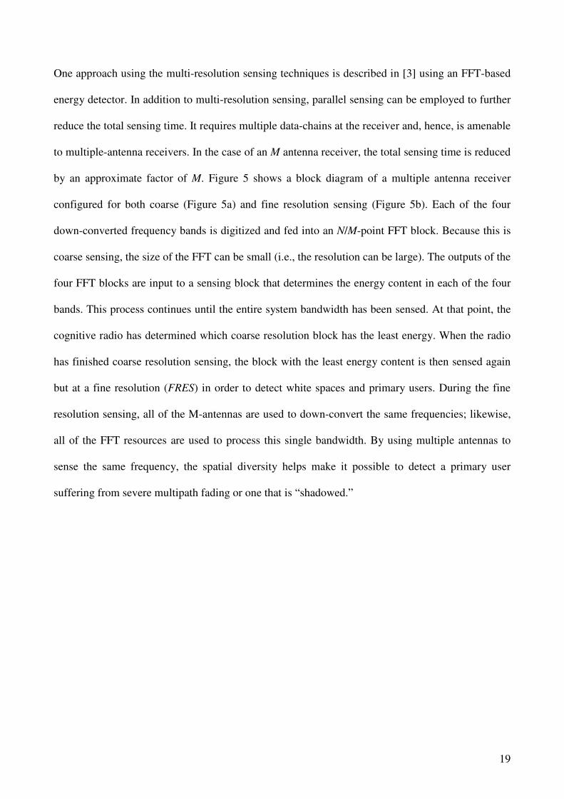
One approach using the multi-resolution sensing techniques is described in [3] using an FFT-based
energy detector. In addition to multi-resolution sensing, parallel sensing can be employed to further
reduce the total sensing time. It requires multiple data-chains at the receiver and, hence, is amenable
to multiple-antenna receivers. In the case of an M antenna receiver, the total sensing time is reduced
by an approximate factor of M. Figure 5 shows a block diagram of a multiple antenna receiver
configured for both coarse (Figure 5a) and fine resolution sensing (Figure 5b). Each of the four
down-converted frequency bands is digitized and fed into an N/M-point FFT block. Because this is
coarse sensing, the size of the FFT can be small (i.e., the resolution can be large). The outputs of the
four FFT blocks are input to a sensing block that determines the energy content in each of the four
bands. This process continues until the entire system bandwidth has been sensed. At that point, the
cognitive radio has determined which coarse resolution block has the least energy. When the radio
has finished coarse resolution sensing, the block with the least energy content is then sensed again
but at a fine resolution (FRES) in order to detect white spaces and primary users. During the fine
resolution sensing, all of the M-antennas are used to down-convert the same frequencies; likewise,
all of the FFT resources are used to process this single bandwidth. By using multiple antennas to
sense the same frequency, the spatial diversity helps make it possible to detect a primary user
suffering from severe multipath fading or one that is “shadowed.”
20
Figure 5. Parallel, multi-resolution system configured for the (a) coarse resolution, and (b) fine
resolution sensing modes
This parallel approach to multiple resolution sensing has shown that for a large number of antennas
(i.e., parallel paths), a smaller coarse resolution sensing bandwidth results in faster sensing times,
whereas for a small number of antennas, a larger coarse resolution sensing bandwidth is preferred.
Furthermore, while the number of points in the FFT gives more flexibility for an OFDM
transceiver, it is better for sensing purposes to have fewer points in the FFT.
1.2.2 MRSS Sensing with wavelet generators
Another MRSS approach with less hardware efforts to implement (antennas and ADC blocks) relies
on analog wideband spectrum sensing and reconfigurable RF front end [4]. In order to provide the
multi-resolution sensing feature the wavelet transform was adopted. This type of transformation is
applied to the input signal and the resulting coefficient values stand for the representation of the
input signal’s spectral contents with the given detection resolution. The spectral components of the
incoming signal are then detected by the Fourier Transform performed in the analog domain. In this
21
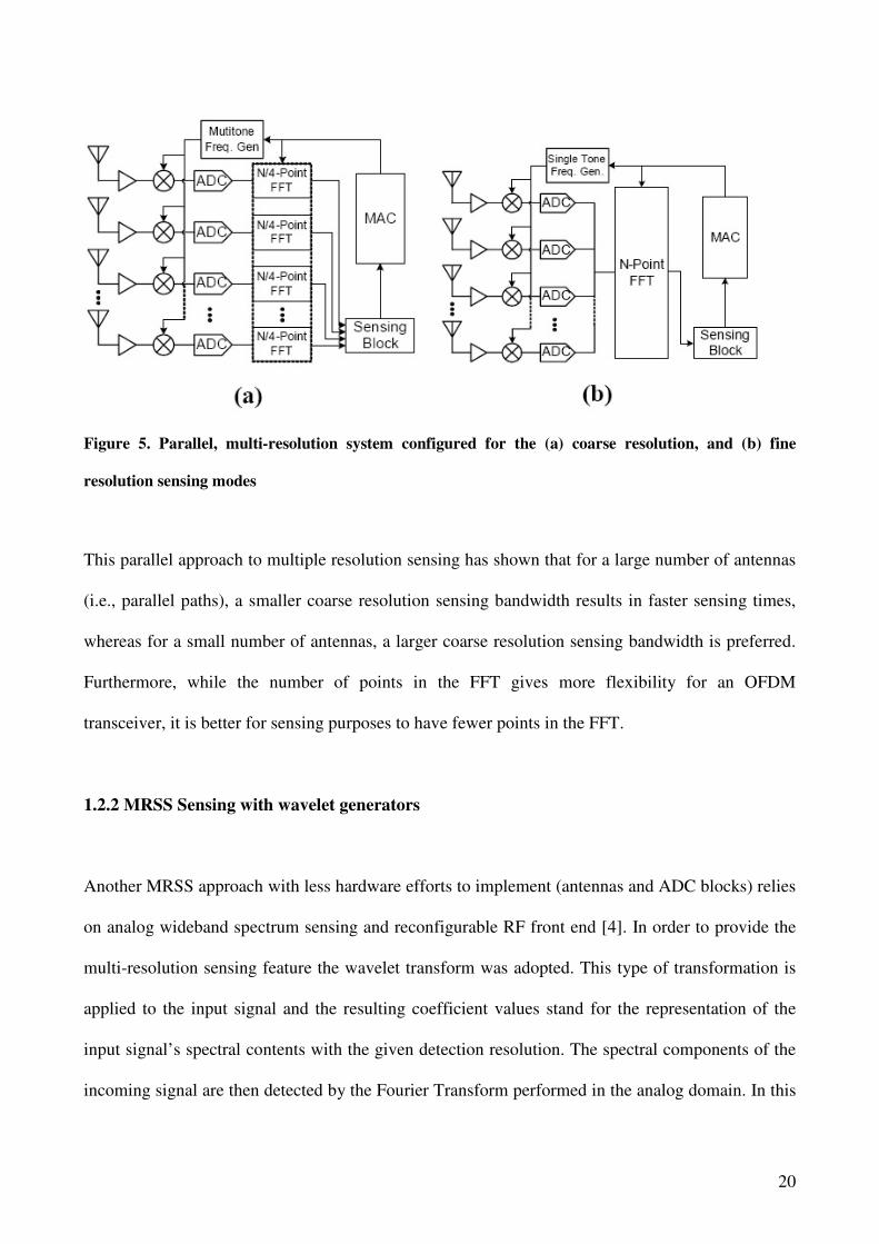
way, bandwidth, resolution and centre frequency can be controlled by wavelet function. A block
diagram of this sensing method is presented in Figure 6.
Figure 6. MRSS with analog wideband spectrum sensing
The building components of this type of MRSS approach consist, as depicted in Figure 6, of an
analog wavelet waveform generator where the wavelet pulse is generated and modulated with I and
Q sinusoidal carrier with the given frequency and a Hann window with 5 MHz bandwidth is
selected as the wavelet. The received signal and the wavelet are multiplied using an analog
multiplier. The frequency of the local oscillator (LO) can sweep within a certain interval for detect
the signal power and the frequency values over the spectrum range of interest. The analog integrator
computes the correlation of the wavelet waveform with the given spectral width, i.e. the spectral
sensing resolution and the resulting correlation with I and Q components of the wavelet waveforms
are inputted to ADC where the values are digitized and recorded. If the correlation values are
greater than the certain threshold level, the sensing scheme determines the meaningful interferer
reception.
Since the analysis is performed in the analog domain, the high speed operation and low power
consumption can be achieved. Furthermore, by applying the narrow wavelet pulse and a large
tuning step size of the frequency of the local oscillator, the MRSS is able to examine a very wide
X ∫ ADC
v(t)*fLO(t)
Driver Amp CLK#2
MAC Timing Clock
Wavelet Generator
CLK#1
x(t)
w(t)
z(t) y(t)

22
spectrum span in the fast and sparse manner. On the contrary, very precise spectrum searching is
realized with the wide wavelet pulse and the delicate adjusting of the local oscillator frequency. In
this manner, by virtue of the scalable feature of the wavelet transform, multi-resolution is achieved
without any additional digital hardware burdens. In addition, unlike the heterodyne based spectrum
analysis techniques, the MRSS does not need any physical filters for image rejection due to the
band pass filtering effect of the window signal.
The disadvantages of this sensing method consist in the difficulty of knowing the frequency
information of received signals which imply relatively complicated hardware comparing to FFT
method. Another disadvantage, still concerning the hardware implementation is the need to generate
wavelet waveform which needs much more complex circuitry than simple oscillator.
1.3 Cyclostationary Feature Detector
Another method for the detection of primary signals is Cyclostationary Feature Detection [2] in
which modulated signals are coupled with sine wave carriers, pulse trains, repeated spreading,
hopping sequences, or cyclic prefixes. This results in built-in periodicity. These modulated signals
are characterized as cyclostationary because their mean and autocorrelation exhibit periodicity. This
periodicity is introduced in the signal format at the receiver so as to exploit it for parameter
estimation such as carrier phase, timing or direction of arrival. These features are detected by
analyzing a spectral correlation function. The main advantage of this function is that it differentiates
the noise from the modulated signal energy. This is due to the fact that noise is a wide-sense
stationary signal with no correlation however modulated signals are cyclostationary due to
embedded redundancy of signal periodicity.
Analogous to autocorrelation function spectral correlation function (SCF) can be defined as:

23
∫∆
∆−∞→∆∞→
−+∆
=2/
2/
* )2/,()2/,(11
limlim)(
t
t
tx dtftXftXt
fS αατ
τττ
α (I.5)
Where the finite time Fourier transform is given by:
∫+
−
−=2
2
2)(),(
τ
τ
πτ
t
t
vujdueuxvtX
(I.6)
Spectral correlation function is also known as cyclic spectrum. While power spectral density (PSD)
is a real valued one dimensional transform, SCF is a complex valued two dimensional transform.
The parameter α is called the cycle frequency. If α = 0 then SCF gives the PSD of the signal.
Because of the inherent spectral redundancy signal selectivity becomes possible. Analysis of signal
in this domain retains its phase and frequency information related to timing parameters of
modulated signals. Due to this, overlapping features in power spectral density are non overlapping
features in cyclic spectrum. Hence different types of modulated signals that have identical power
spectral density can have different cyclic spectrum.
Figure 7. Block diagram of a cyclostationary feature detector
Implementation of a spectrum correlation function for cyclostationary feature detection is depicted
in Figure 7. It can be designed as augmentation of the energy detector from Figure 4 with a single
correlator block. Detected features are number of signals, their modulation types, symbol rates and
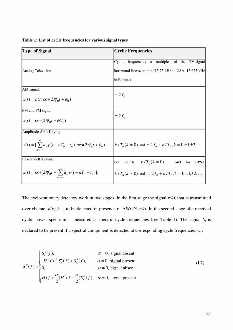
presence of interferers. Table 1 presents examples of the cyclic frequencies adequate for the most
common types of radio signals [4].
A/D
Correlate
X(f+a)X*(f-a)
N pt. FFT
Feature
detect
x(t) Average
over T
24
Table 1: List of cyclic frequencies for various signal types
Type of Signal Cyclic Frequencies
Analog Television
Cyclic frequencies at multiples of the TV-signal
horizontal line-scan rate (15.75 kHz in USA, 15.625 kHz
in Europe)
AM signal:
)2cos()()( 00 φπ += tftatx 02 f±
PM and FM signal:
))(2cos()( 0 ttftx φπ += 02 f±
Amplitude-Shift Keying:
)2cos(])([)( 0000 φπ +−−= ∑∞
−∞=
tftnTtpatxn
n
)0(/ 0 ≠kTk and K,2,1,0,/2 00 ±±=+± kTkf
Phase-Shift Keying:
].)(2cos[)( 000 ∑∞
−∞=
−−+=n
n tnTtpatftx π
For QPSK, )0(/ 0 ≠kTk , and for BPSK
)0(/ 0 ≠kTk and K,2,1,0,/2 00 ±±=+± kTkf
The cyclostationary detectors work in two stages. In the first stage the signal x(k), that is transmitted
over channel h(k), has to be detected in presence of AWGN n(k). In the second stage, the received
cyclic power spectrum is measured at specific cycle frequencies (see Table 1). The signal Sj is
declared to be present if a spectral component is detected at corresponding cycle frequencies αj .
(I.7)
0
2 0 0
*
( ), 0, signal absent
| ( ) | ( ) ( ), 0, signal present
( ) 0, 0, signal absent
( ) ( )2 2
n
s n
x
s
S f
H f S f S f
S f
H f H f S
α
α
α
α
α α
=
+ =
≠
+ −
=
( ), 0, signal presentfα α
≠

25
Among the advantages of the cyclostationary feature detection we can enumerate the robustness to
noise because stationary noise exhibits no cyclic correlations, better detector performance even in
low SNR regions, the signal classification ability and the flexibility of operation because it can be
used as an energy detector in α = 0 mode.
The disadvantages are a more complex processing needed than energy detection and therefore high
speed sensing can not be achieved. The method cannot be applied for unknown signals because an a
priori knowledge of target signal characteristics is needed. Finally, at one time, only one signal can
be detected: for multiple signal detection, multiple detectors have to be implemented or slow
detection has been allowed.
1.4 Mixed mode sensing schemes
Since cyclostationary feature detection is somehow complementary to the energy detection,
performing better for narrow bands, a combined approach is suggested in [4], where energy
detection could be used for wideband sensing and then, for each detected single channel, a feature
detection could be applied in order to make the final decision whether the channel is occupied or
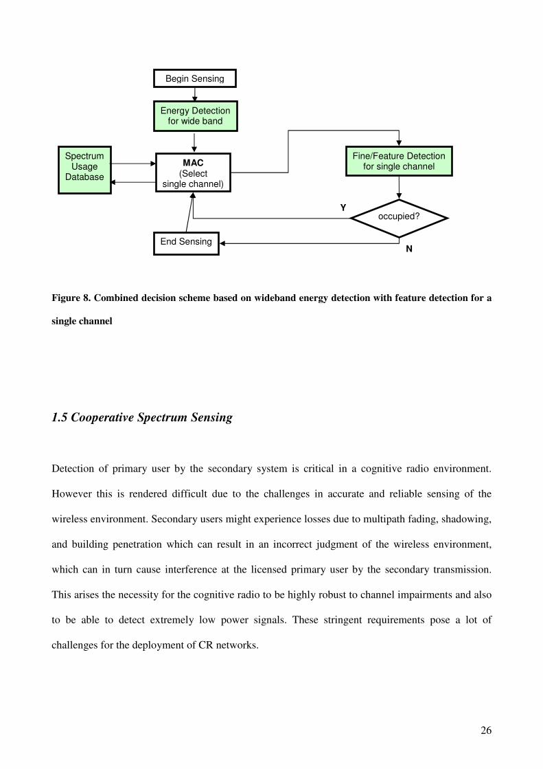
not. Such a decisional architecture is presented in Figure 8. First a coarse energy detection stage is
performed over a wider frequency. Subsequently the presumed free channel is analyzed with the
feature detector in order to take the decision.
26
Figure 8. Combined decision scheme based on wideband energy detection with feature detection for a
single channel
1.5 Cooperative Spectrum Sensing
Detection of primary user by the secondary system is critical in a cognitive radio environment.
However this is rendered difficult due to the challenges in accurate and reliable sensing of the
wireless environment. Secondary users might experience losses due to multipath fading, shadowing,
and building penetration which can result in an incorrect judgment of the wireless environment,
which can in turn cause interference at the licensed primary user by the secondary transmission.
This arises the necessity for the cognitive radio to be highly robust to channel impairments and also
to be able to detect extremely low power signals. These stringent requirements pose a lot of
challenges for the deployment of CR networks.
Energy Detection for wide band
Begin Sensing
Fine/Feature Detection for single channel
End Sensing
occupied? Y
N
MAC (Select
single channel)
Spectrum Usage
Database

27
1.6 Cooperative techniques
High sensitivity requirements on the cognitive user caused by various channel impairments and low
power detection problems in CR can be alleviated if multiple CR users cooperate in sensing the
channel. [5] suggests different cooperative topologies which can be broadly classified into three
regimes according to their level of cooperation.
1.6.1 Decentralized Uncoordinated Techniques
The cognitive users in the network don’t have any kind of cooperation which means that each CR
user will independently detect the channel, and if a CR user detects the primary user it would vacate
the channel without informing the other users. Uncoordinated techniques are fallible in comparison
with coordinated techniques. Therefore, CR users that experience bad channel realizations
(shadowed regions) detect the channel incorrectly thereby causing interference at the primary
receiver.
1.6.2 Centralized Coordinated Techniques
In these kinds of networks, an infrastructure deployment is assumed for the CR users. CR user that
detects the presence of a primary transmitter or receiver informs a CR controller. The CR controller
can be a wired immobile device or another CR user. The CR controller notifies all the CR users in
its range by means of a broadcast control message. Centralized schemes can be further classified in
according to their level of cooperation into (a) Partially Cooperative: in partially cooperative
networks nodes cooperate only in sensing the channel. CR users independently detect the channel
inform the CR controller which then notifies all the CR users. One such partially cooperative
scheme was considered by [6] where a centralized Access Point (CR controller) collected the
sensory information from the CR users in its range and allocated spectrum accordingly; (b) Totally
Cooperative Schemes: in totally cooperative networks nodes cooperate in relaying each others

28
information in addition to cooperatively sensing the channel. For example, the cognitive users D1
and D2 are assumed to be transmitting to a common receiver and in the first half of the time slot
assigned to D1, D1 transmits and in the second half D2 relays D1’s transmission. Similarly, in the
first half of the second time slot assigned to D2, D2 transmits its information and in the second half
D1 relays it.
1.6.3 Decentralized Coordinated Techniques
Various algorithms have been proposed for the decentralized techniques, among which the
gossiping algorithms [7], which do cooperative sensing with a significant lower overhead. Other
decentralized techniques rely on clustering schemes [8] where cognitive users form in to clusters
and these clusters coordinate amongst themselves, similar to other already known sensor network
architecture (i.e. ZigBee).
Figure 9. Cooperation Techniques among CR. (a) decentralized coordination technique and
centralized coordinated techniques as (b) partial or (c) total cooperative
All these techniques for cooperative spectrum sensing, graphically illustrated in Figure 9, raise the
need for a control channel [8] which can be either implemented as a dedicated frequency channel or
as an underlay UWB channel. Wideband RF front-end tuners/filters can be shared between the

29
UWB control channel and normal cognitive radio reception/transmission. Furthermore, with
multiple cognitive radio groups active simultaneously, the control channel bandwidth needs to be
shared. With a dedicated frequency band, a CSMA scheme may be desirable. For a spread spectrum
UWB control channel, different spreading sequencing could be allocated to different groups of
users.
1.7 Benefits of cooperation
Cognitive users selflessly cooperating to sense the channel has a lot of benefits among which we
can mention:
Plummeting Sensitivity Requirements: Channel impairments like multipath fading, shadowing
and building penetration losses impose high sensitivity requirements on cognitive radios. However
sensitivity of cognitive radio is inherently limited by cost and power requirements. Also due to the
statistical uncertainties in noise and signal characteristics there is a lower bound on the minimum
power that a CR user can detect, called the SNR wall. It has been shown that the sensitivity
requirement can be drastically reduced by employing cooperation between nodes. All the
cooperative topologies that we considered in the earlier section provide sensitivity benefits. For
example, in [10] the sensitivity benefits obtained from a partially cooperative coordinated
centralized scheme showed a -25 dBm reduction in sensitivity threshold obtained by using this
scheme.
Agility Improvement Using Totally Cooperative Centralized Coordinated Scheme: One of the
biggest challenge in cognitive radio is reduction of the overall detection time. All topologies of
cooperative networks in general reduce detection time compared to uncoordinated networks.

30
However the totally cooperative centralized schemes have been shown to be highly agile of all the
cooperative schemes. They have been shown to be over 35 % more agile compared tot the partially
cooperative schemes. Totally cooperative schemes achieve high agility by pairing up “weak users”
with “strong ones”. For example [10] if an user U1 hears very low primary signal as it’s close to the
boundary of decidability then it increases the detection time for U1. If an U2 user is much closer to
the primary user, it will hear a strong primary user signal, and when it relays U1’s transmission the
CR controller detects the presence of the primary user thereby reducing detection time when
compared to ordinary cooperative networks. Even though the benefits don’t seem significant, it
should be remembered that cooperative sensing has to be performed frequently and even small
benefits will have a large impact on system performance.
Cognitive Relaying: With the number of CR users going up, the probability of finding spectrum
holes will reduce drastically with time. CR users would have to scan a wider range of spectrum to
find a hole resulting in undesirable overhead and system requirements. An alternative solution to
this is Cognitive Relaying proposed by [10]. In cognitive relaying the secondary user selflessly
relays the primary users transmission thereby diminishing the primary users transmission time.
Thus cognitive relaying in effect creates “spectrum holes”. However this method might not be
practical due to many reasons. The primary user wouldn’t let the secondary user decode its
transmission due to security related issues. Also since the cognitive users are generally ad hoc
energy constrained devices, they might not relay primary users transmission. Even though cognitive
relaying has the following disadvantages it is a very good way of creating transmission
opportunities when spectrum gets scarce.
1.8 Disadvantages of cooperation
Cooperative sensing in the aforementioned schemes is not trivial due to the following factors:

31
Limited Bandwidth: CR users are low cost low power devices that might not have dedicated
hardware for cooperation. Therefore data and cooperation information have to be multiplexed
causing degradation of throughput for the cognitive user.
Short Timescales: The CR user have to do sensing at periodic intervals as sensed information
become obsolete fast due to factors like mobility, channel impairments etc.. This considerably
increases the data overhead.
Large Sensory Data: Since the cognitive radio can potentially use any unused spectrum hole, it
will have to scan a wide range of spectrum, resulting in large amounts of data. This is inefficient in
terms of data throughput, delay sensitivity requirements and energy consumption for the cognitive
users.
Scalability: Scalability is a big issue in cooperation. Even though cooperation has its benefits, too
many users cooperating can have adverse effects. It was shown in [10] that partially cooperative
centralized coordinated schemes follow the law of diminishing returns as the number of users goes
up. In [12] a totally cooperative centralized coordinated scheme was considered where benefits of
cooperation increased with the number of nodes participating. In this scheme a “weaker user” was
always paired with a “stronger user” using a decentralized algorithm making the scheme scalable.
Even though this network has been shown to be scalable, the algorithm makes a lot of assumptions
which might not be true in any wireless network. For example, this scheme assumes a “distance
symmetric” distribution of nodes to make pairing possible.
Even though cooperatively sensing data poses a lot of challenges, it could be carried out without
incurring much overhead. This is mainly because only an approximate sensing information is

32
required thereby eliminating the need for complex signal processing schemes at the receiver and
reducing the data load. Also even though a wide channel has to be scanned, only a portion of it
changes at a time, requiring updating only the changed information and not the details of the entire
scanned spectrum. Scalability issues in cooperative sensing can be resolved by considering more
distributed cooperative algorithms. This is an extensively researched area in general ad hoc
networks and also sensor networks.
1.9 Sensor networks for spectrum sensing
A different approach for cooperative spectrum sensing involves a sensor network based sensor
architecture [9]. The idea behind this sensor network based sensing architecture is to have a separate
sensor network fully dedicated to perform spectrum sensing. In this architecture, at least two types
of networks are identified: the sensing network and one or more operational net works. The sensing
network would be comprised of a set of sensors deployed in the desired target area and which
would sense the spectrum (either continuously or periodically) and communicate the results (which
may be subjected to some processing such as data fusion, etc.) to a well-known sink node. The sink
node may, in turn, further process the collected data and will eventually make the information about
the spectrum occupancy in the sensed target area available to all operational net-works. The
operational networks, on the other hand, are responsible for traditional data transmission and
opportunistic use of the spectrum, and would accept the information about the spectrum occupancy
map in order to determine which channel to use, when to use, and for how long.
This architecture offers some benefits, mainly consisting in the fact that the measurements made in
a network provide the needed diversity to cope with multipath fading and other signal loss
problems. By separating the sensing and operational functions, using this architecture, no lost
transmit opportunity costs are incurred. Finally, since operational networks need to be mobile and
may be power limited, whereas the sensing function does not need to be mobile, this architecture
33
brings unique power advantages, especially to low power portable/mobile applications. Of course,
the main disadvantage of this approach is the need of deploying this architecture in some manner,
which raises some questions about sustainability and is limiting, at least for now, the application
domain of the approach.
1.10 Design of a Spectrum Sensing System using the DWPT transformation
An initial algorithm for spectrum sensing and communication using DWPT was developed for the
IEEE SCC41-P19006 Meeting in Chicago, October 2008.
In chapter IV is described a new algorithm for sensing spectrum trough DWPT.

34
Chapter II
State of the art on cognitive radio transmission
With the demand for additional bandwidth increasing due to existing and new services, new
solutions are sought for this apparent spectrum scarcity. Although measurement studies have shown
that licensed spectrum is relatively unused across time and frequency, current government
regulatory requirements prohibit unlicensed transmissions in these bands, constraining them instead
to several heavily populated, interference-prone frequency bands. To provide the necessary
bandwidth required by current and future wireless services and applications, a new concept of
unlicensed users ”borrowing” spectrum from spectrum licensees, known as dynamic spectrum
access (DSA) is born.
Simultaneously, the development of software, defined radio (SDR) technology, where the radio
transceivers perform the baseband processing entirely in software, which made them a prime
candidate for DSA networks due to their ease and speed of programming baseband operations. SDR
units that can rapidly reconfigure operating parameters due to changing requirements and
conditions1 are known as cognitive radios (CR).
In a CR environment, there are two types of terminals [1]: primary (or licensed) terminals, which
have the right to access the spectral resources any time, including GPRS, UMTS, emergency
services, broadcast TV; and secondary (or CR) terminals, which seek transmission opportunities by
exploiting the idle periods or unused spectrum of the primary system.
Primary users take up most of the spectrum, and CR users can use their unused spectrum
opportunistically. The CR terminals are assumed to be able to detect any unoccupied frequencies

35
and to estimate the strength of the received signal of nearby primary users by spectrum sensing so
that they can infer the signal to noise ratio (SNR) of the primary users. The CR terminals are also
assumed to be equipped with extra RF circuits only for sensing, so they can communicate using a
carrier frequency and sense adjacent frequencies at the same time. The CR user is assumed to be
able to sense the reappearance of a primary user in the frequency in use by monitoring the
degradation of his SNR in the downlink. Once a CR user detects free frequency spectrum within the
licensed frequency range, he may negotiate with the primary system, or begin data transmission
without extra permission, depending on the CR system structure. If any primary users become
active in the same frequency band later on, the CR user has to clear this band as soon as possible,
giving priority to the primary users. Also, CR users should quit their communication if the
estimated SNR levels of the primary users are below an acceptable level. When a CR user operates
in a channel adjacent to any active primary users’ spectrums, ACI occurs between the two parties.
However, the performance of the primary system should be maintained, whether spectrum sharing
is allowed or not. We assume that a minimum SNR requirement is predefined for the primary
system so that the maximum allowable ACI at each location can be evaluated by the CR user. The
CR user can then determine whether he may use the frequency band or not. At the same time, the
CR user needs to avoid the influence of interference from primary users in order to maximize its
own data throughput.
Other properties of his type of radio are the ability to operate at variable symbol rates, modulation
formats (e.g. low to high order QAM), different channel coding schemes, power levels and the use
of multiple antennas for interference nulling, capacity increase or range extension (beam forming).
The most likely basic strategy will be based on OFDM-like modulation across the entire bandwidth
in order to most easily resolve the frequency dimension with subsequent spatial and temporal
processing.

36
2.1 Modulation formats
The choice of a physical layer data transmission scheme is a very important design decision when
implementing a cognitive radio. Specifically, the technique must be sufficiently agile to enable
unlicensed users the ability to transmit in a licensed band while not interfering with the incumbent
users. Moreover, to support throughput-intensive applications, the technique should be capable of
handling high data rates.
2.1.1 OFDM
The modulation scheme based on orthogonal frequency division multiplexing (OFDM) is a natural
approach that might satisfy desired properties [1]. OFDM has become the modulation of choice in
many broadband systems due to its inherent multiple access mechanism and simplicity in channel
equalization, plus benefits of frequency diversity and coding. The transmitted OFDM waveform is
generated by applying an inverse fast Fourier transform (IFFT) on a vector of data, where number
of points N determines the number of sub-carriers for independent channel use, and minimum
resolution channel bandwidth is determined by W/N, where W is the entire frequency band
accessible by any cognitive user.
The frequency domain characteristics of the transmitted signal are determined by the assignment of
non-zero data to IFFT inputs corresponding to sub-carriers to be used by a particular cognitive user.
Similarly, the assignment of zeros corresponds to channels not permitted to use due to primary user
presence or channels used by other cognitive users. The output of the IFFT processor contains N
samples that are passed through a digital-to-analog converter producing the wideband waveform of
bandwidth W. A great advantage of this approach is that the entire wideband signal generation is

37
performed in the digital domain, instead of multiple filters and synthesizers required for the signal
processing in analog domain.
From the cognitive network perspective, OFDM spectrum access is scalable while keeping users
orthogonal and non-interfering, provided the synchronized channel access. However, this
conventional OFDM scheme does not provide truly band-limited signals due to spectral leakage
caused by sinc-pulse shaped transmission resulted from the IFFT operation. The slow decay of the
sinc-pulse waveform, with first side lobe attenuated by only 13.6dB, produces interference to the
adjacent band primary users which is proportional to the power allocated to the cognitive user on
the corresponding adjacent sub-carrier. Therefore, a conventional OFDM access scheme is not an
acceptable candidate for wideband cognitive radio transmission.
[2] suggests non contiguous OFDM, NC-OFDM as an alternative, a schematic of an NC-OFDM
transceiver being shown in Figure 10. The transceiver splits a high data rate input, x(n), into N
lower data rate streams. Unlike conventional OFDM, not all the sub carriers are active in order to
avoid transmission unoccupied frequency bands. The remaining active sub carriers can either be
modulated using M-ary phase shift keying (MPSK), as shown in the figure, or M-ary quadrature
amplitude modulation (MQAM). The inverse fast Fourier transform (IFFT) is then used to
transform these modulated sub carrier signals into the time domain. Prior to transmission, a guard
interval, with a length greater than the channel delay spread, is added to each OFDM symbol using
the cyclic prefix (CP) block in order to mitigate the effects of inter-symbol interference (ISI).
Following the parallel-to-serial (P/S) conversion, the base band NC-OFDM signal, s(n), is then
passed through the transmitter radiofrequency (RF) chain, which amplifies the signal and
upconverts it to the desired centre frequency. The receiver performs the reverse operation of the
transmitter, mixing the RF signal to base band for processing, yielding the signal r(n). Then the
signal is converted into parallel streams, the cyclic prefix is discarded, and the fast Fourier
transform (FFT) is applied to transform the time domain data into the frequency domain. After the
distortion from the channel has been compensated via per sub carrier equalization, the data on the

38
sub carriers is demodulated and multiplexed into a reconstructed version of the original high-speed
input, )(nx)
.
NC-OFDM was evaluated and compared, both qualitatively and quantitatively with other candidate
transmission technologies, such as MC-CDMA and the classic OFDM scheme. The results show
that NC-OFDM is sufficiently agile to avoid spectrum occupied by incumbent user transmissions,
while not sacrificing its error robustness.
Figure 10. Schematic of an NC – OFDM transceiver
2.1.2 Adaptive modulation
Adaptive modulation is only appropriate for duplex communication between two or more stations
because the transmission parameters have to be adapted using some form of a two-way transmission
in order to allow channel measurements and signalling to take place. Transmission parameter
adaptation is a response of the transmitter to the time-varying channel conditions. In order to
efficiently react to the changes in channel quality, the following steps need to be taken:

39
1) Channel quality estimation: To appropriately select the transmission parameters to be
employed for the next transmission, a reliable estimation of the channel transfer function
during the next active transmit slot is necessary. This is done at the receiver and the
information about the channel quality is sent to the transmitter for next transmission through
a feedback channel.
2) Choice of the appropriate parameters for the next transmission: Based on the prediction of
the channel conditions for the next time slot, the transmitter has to select the appropriate
modulation modes for the sub-carriers.
3) Signalling or blind detection of the employed parameters: The receiver has to be informed,
as to which demodulator parameters to employ for the received packet.
In a scenario where channel conditions fluctuate dynamically, systems based on fixed modulation
schemes do not perform well, as they cannot take into account the difference in channel conditions.
In such a situation, a system that adapts to the worst case scenario would have to be built to offer an
acceptable bit-error rate. To achieve a robust and a spectrally efficient communication over multi-
path fading channels, adaptive modulation is used, which adapts the transmission scheme to the
current channel characteristics. Taking advantage of the time-varying nature of the wireless
channels, adaptive modulation based systems alter transmission parameters like power, data rate,
coding, and modulation schemes, or any combination of these in accordance with the state of the
channel. If the channel can be estimated properly, the transmitter can be easily made to adapt to the
current channel conditions by altering the modulation schemes while maintaining a constant BER.
This can be typically done by estimating the channel at the receiver and transmitting this estimate
back to the transmitter. Thus, with adaptive modulation, high spectral efficiency can be attained at a
given BER in good channel conditions, while a reduction in the throughput is experienced in
degrading channel conditions [3]. The basic block diagram of an adaptive modulation based

40
cognitive radio system is shown in Figure 11. The block diagram provides a detail view of the
whole adaptive modulation system with all the necessary feedback paths.
Figure 11. Basic block diagram of an adaptive modulation - based cognitive radio system
It is assumed that the transmitter has a perfect knowledge of the channel and the channel estimator
at the receiver is error-free and there is no time delay. The receiver uses coherent detection methods
to detect signal envelopes. The adaptive modulation, M-ary PSK, M-QAM, and M-ary AM schemes
with different modes are provided at the transmitter. With the assumption that the estimation of the
channel is perfect, for each transmission, the mode is adjusted to maximize the data throughput
under average BER constraint, based on the instantaneous channel SNR. Based on the perfect
knowledge about the channel state information (CSI), at all instants of time, the modes are adjusted
to maximize the data throughput under average BER constraint.
The data stream, b(t)is modulated using a modulation scheme given by )(γ)
kP , the probability of
selecting kth
modulation mode from K possible modulation schemes available at the transmitter,
TRANSMITTER
BER
CALCULATOR
MODULATION
SELECTION
RECEIVER DETECTION
MODULATOR
CHANNEL
ESTIMATOR
x +
Data Input b x
γ
y
h
b
h(t) AWGN,w(t)
P(γ)

41
which is a function of the estimated SNR of the channel. Here, h(t) is the fading channel and w(t) is
the AWGN channel. At the receiver, the signal can be modelled as:
y(t) = h(t) x(t) + w(t) (II.1)
where y(t) is the received signal, h(t) is the fading channel impulse response, and w(t) is the
Additive White Gaussian Noise (AWGN). The estimated current channel information is returned to
the transmitter to decide the next modulation scheme. The channel state information, )(th)
is also
sent to the detection unit to get the detected stream of data, )(tb)
2.2 Power Scaling
One of the most challenging problems of cognitive radio is the interference, which occurs when a
cognitive radio accesses a licensed band but fails to notice the presence of the licensed user. To
address this problem, the cognitive radio should be designed to co-exist with the licensed user
without creating harmful interference. Recently, several interference mitigation techniques have
been presented for cognitive radio systems. An orthogonal frequency division multiplexing
(OFDM) was considered as a candidate for cognitive radio to avoid the interference by leaving a set
of sub channels unused. Thus, it can provide a flexible spectral shape that fills the spectral gaps
without interfering with the licensed users. A transform domain communication system (TDCS)
was proposed to mitigate the interference by not putting the waveform energy at corrupted spectral
locations. A power control rule was presented to allow cognitive radios to adjust their transmit
powers in order to guarantee a quality of service to the primary system. To avoid the interference to
the licensed users, the transmit power of the cognitive radio should be limited based on the
locations of the licensed users. However, it is difficult to locate the licensed users for the cognitive

42
radio in practice because the channels between the cognitive radio and the licensed users are usually
unknown. Furthermore, the environment where the system is in operation may have large delay
spread and hence the channel model is complicated by fading, shadowing and path loss effects. In
[4], the local oscillator (LO) leakage power was exploited to locate the primary receivers. But it is
still not easy to apply this in practice because the approach requires a sensor node mounted close to
the primary receivers to detect the LO leakage power.
Another power control approach in cognitive radio systems is based on spectrum sensing side
information in order to mitigate the interference to the primary user due to the presence of cognitive
radios [5]. This approach consists of two steps. Firstly, the shortest distance between a licensed
receiver and a cognitive radio is derived from the spectrum sensing side information. Then, the
transmit power of the cognitive radio is determined based on this shortest distance to guarantee a
quality of service for the licensed user. Because the worst case is considered in this approach where
the cognitive radio is the closest to the licensed user, this power control approach can be applied to
the licensed user in any location.
In [6], the transmission power and position of the primary user in CR is considered due to the fact
that information of the primary user determines the spatial resource. To find position of the primary
user, various attempts try to use existing positioning or localization schemes based on ranging
techniques but those schemes require the primary user’s transmission. Since most primary users in
CR are legacy system, and there are no beacon protocol to advertise useful information such as
transmission power. [6] proposes the constrained optimization method to estimate transmission
power and position without the prior information of the transmission power. The proposed scheme
use the linearization technique to approximate relationship between RSS measurements and
unknown power and coordinates of the primary user to set weighting factor that considers the
differences of the quality of measurements, and then applies the constrained optimization method
containing appropriate weighting factor.

43
The system model used for this method is illustrated in Figure 12, which represents the network
configuration for position and transmission power estimation in CR. Primary users are emitting the
signal through air, and the secondary users are receiving the signal from the primary users. A bold
dotted line denotes the primary user’s signal. Secondary users share the information of measured
RSS values at each user and position of users. Dotted lines are secondary user’s communications to
share the information.
Figure 12. Network configuration for a method for robust transmission power and position estimation
in cognitive radio
The method implies some assumptions under which secondary users can estimate the unknown
primary users’ position and transmission power. These assumptions are:
� primary users’ transmission powers are unknown
� secondary users’ positions are known
� secondary users measure the RSS values from primary users
44
� there are at least 4 secondary users receiving the signal from the primary user
� a shadowing effect to each secondary user is independent
2.3 Radio design architectures
2.3.1 Antenna issues
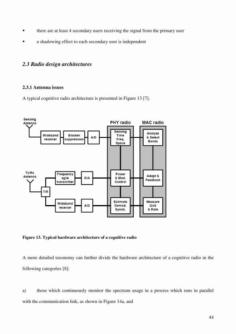
A typical cognitive radio architecture is presented in Figure 13 [7].
Figure 13. Typical hardware architecture of a cognitive radio
A more detailed taxonomy can further divide the hardware architecture of a cognitive radio in the
following categories [8]:
a) those which continuously monitor the spectrum usage in a process which runs in parallel
with the communication link, as shown in Figure 14a, and

45
b) those which use a single channel for both spectrum sensing and communication, as shown in
Figure 14b
In category (a), systems have been proposed that use two antennas. One antenna is wideband and
omni-directional, feeding a receiver capable of both coarse and fine spectrum sensing over a broad
bandwidth. The second antenna is directional and feeds a frequency agile transmitter that can be
tuned to the selected band. Category (a) also includes single antenna systems, where a single
wideband antenna feeds both the spectrum sensing modules and the frequency agile front end.
Figure 14. Radio architectures with parallel (a) and combined sensing and communication (b).
In category (b), spectrum sensing and radio reconfiguration are performed when the communication
link quality falls below defined thresholds. In [8], two thresholds are used. Link quality falling
below the first threshold triggers spectrum sensing, so that a better system configuration can be
identified that will meet the link quality requirements. When the quality degrades below a second
lower threshold, the system is reconfigured.
An important issue in the front-end architecture is to limit the instantaneous dynamic range to avoid
non-linear distortion of signals in the wanted channel. Many authors envisage the use of tunable
filters to reduce interference and therefore limit the dynamic range. Interference can also be limited

46
by the use of directional antenna properties. In [9], a simple switched pattern technique was
described which could limit interference from primary sources whilst maintaining communications
between users in the local network, enhanced by a multi-hop approach. In addition, the use of a
switched wide band directional antenna, combining spatial and spectral discrimination may also be
useful.
Whether both of these techniques are used depends on available space. In the case of a base station
both spatial and spectral sensing may be used, but in the case of handheld terminals it is likely that
only spectral sensing may be possible. There are significant antenna challenges in such systems.
� in general wideband antennas are bigger than narrowband ones, which will be a significant
problem for handsets;
� the design of wideband arrays for base stations gives great difficulties in element spacing;
� narrowband antennas provide a degree of pass band filtering, which, by supplementing the
filtering in the RF stages, provides control of the noise level, which is mainly determined by
interference;
� the fundamental limits of electrically small antennas, in terms of bounds on Q factor and
gain, also limit the instantaneous coverage that can be achieved. Combining these two
bounds implies that an antenna with an extremely wide band will be very inefficient, if it is
small compared to the wavelength. This will limit the sensitivity for search.
From the system considerations discussed above, some novel antenna configurations are
investigated for their feasibility [8]. It has been examined how a narrow band and a wideband
antenna may be integrated into the same volume, and then demonstrated how external tuning
circuits can be used to tune the narrow band antenna over the wide bandwidth and also to switch
between wideband and narrowband operation.

47
2.3.2 Multi-transmission methods
For implementation of cognitive radio, multi-transmission methods based on packet communication
is one of the most promising alternatives because it considers the shift of the all IP network
architecture. The multi-transmission method [10] can be realized within the current wireless
regulations and improves the efficiency of frequency utilization. An example of this type of
transmission is presented in Figure 15.
Figure 15. Multi – transmission architecture
The wireless modules of 3G cellular, mobile Wi-MAX and WLAN supporting the MAC sub-layer
to the LLC sub-layer are accommodated in a single base station and connected to each other with a
Layer 2 switch. With the Layer 2 switch, a processor bundles the multiple MACs of the wireless
modules into a single virtual MAC. The MAC convergence processor, installed in the base station
and in the user terminal, connected to the I/F modules of the base station router and the I/F modules
of the host, respectively.

48
The MAC convergence processor has two functions. When it sends a packet to the peer, it adds a
cognitive header to the packets coming from the router or host, in order to establish an inter-
wireless system session with the other node. It also adds the header to feed the packets to the proper
wireless module physically linked to the peer. The Layer 2 switch directs the large number of
packets to the proper wireless module immediately after detecting the MAC address of the receiving
packets. When receiving the packets, the processor removes the cognitive header from the receiving
packets from the Layer 2 switch, aligns the packets in the right order without reversion in
accordance with the sequence number in the header, and sends them to the router or the host I/F.
The advantages of this approach are low cost and scalability. The following five functions are
required to enable cognitive radio with the multi-transmission scheme:
� integration scheme for wireless media inside the wireless station;
� numerical recognition of wireless capacity;
� long term and short term prediction method for wireless traffic changes;
� packet switch to select the optimum wireless media;
� optimization protocol between wireless nodes within the wireless area.
The multi-transmission link method together with virtual MACs and the radio environment
recognition method were verified by an experiment using a WLAN system as wireless sensors to
detect the wireless available capacities. The proposed system is composed of existing technologies
and does not require the development of special devices. Therefore, this system can be deployed for
cognitive radio architectures and is applicable to wireless traffic congested metropolitan areas [10].
2.3.3 High performance, multi – band implementation
An interesting cognitive radio architecture presented in [11] is aimed at providing a high-
performance platform with various adaptive wireless network protocols ranging from simple

49
etiquettes to more complex ad-hoc collaboration. Particular emphasis has been placed on high
performance in a networked environment where each node may be required to carry out high
throughput packet forwarding functions between multiple physical layers. Key design objectives for
the cognitive radio platform include:
� multi-band operation, fast frequency scanning and agility;
� software-defined modem including waveforms such as DSSS/QPSK and OFDM operating
at speeds up to 50 Mbps;
� packet processor capable of ad-hoc packet routing with aggregate throughput ~100 Mbps;
� spectrum policy processor that implements etiquette protocols and algorithms for dynamic
spectrum sharing.
The radio architecture is based on four major elements: (1) MEMS-based tri-band agile RF front-
end; (2) FPGA-based software defined radio (SDR); (3) FPGA-based packet processing engine; and
(4) embedded CPU core for control and management. The basic design, illustrated in Figure 16
provides for fast RF scanning capability, an agile RF transceiver working over a range of frequency
bands, a software-defined radio modem capable of supporting a variety of waveforms including
OFDM and DSSS/QPSK, a packet processing engine for protocol and routing functionality, and a
general purpose processor for implementation of spectrum etiquette policies and algorithms. The
presented implementation was equipped with 3 radio front-end blocks, working in the 900 MHz, 2.4
GHz and the 5.2 GHz radio bands.
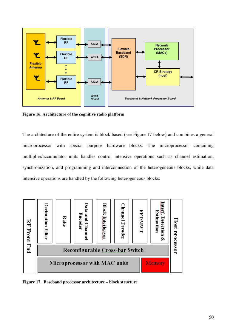
50
Figure 16. Architecture of the cognitive radio platform
The architecture of the entire system is block based (see Figure 17 below) and combines a general
microprocessor with special purpose hardware blocks. The microprocessor containing
multiplier/accumulator units handles control intensive operations such as channel estimation,
synchronization, and programming and interconnection of the heterogeneous blocks, while data
intensive operations are handled by the following heterogeneous blocks:
Figure 17. Baseband processor architecture – block structure
Flexible RF
Flexible RF
Flexible RF
Flexible Baseband
(SDR)
Network Processor
(MAC+)
CR Strategy (host)
Flexible Antenna
A/D/A
A
Baseband & Network Processor Board
Antenna & RF Board
A/D/A
Board
A/D/A
A
A/D/A
A

51
1. Channelization Block: A configurable multi-stage filter used to select a sub-band and/or
decimate the input signal for different standards.
2. FFT/MWT Block: A configurable architecture, which can handle FFT operations used in
OFDM and also handle, the modifier Walsh transform used in 802.11b.
3. Rake Block: A generic four finger Rake accelerator for channel estimation, de-spreading in
DSSS and CDMA.
4. Interleaver Block: Using a block-based memory and multiplexer-based address handler, a
multi-mode architecture can handle de-interleaving for different standards.
5. Data and Channel Encoding /Decoding Block: A configurable architecture can handle both
Viterbi (for 802.11a) and Encoder/Turbo Decoder (for WCDMA). Both the Data and
Channel Encoder have a similar connection pattern, but only the Data Encoder needs
feedback. A common block is proposed which can be configured in one clock cycle to
perform either of the two functionalities.
6. Detection and Estimation Block: Common interference detection block.
2.4 Design of a transmission system using the WPDM
After reviewing the modulations presented in chapter 2.1, we focused on using the Wavelet Packet
Division Multiplex technique, combined with Binary Phase Shift Keying (BPSK) and Pulse-
Amplitude Modulation (PAM).
2.4.1 Theoretical background
The theoretical background relies on the synthesis of the discrete wavelet packet transform that
constructs a signal as the sum of M = 2J waveforms. Those waveforms can be built by J successive
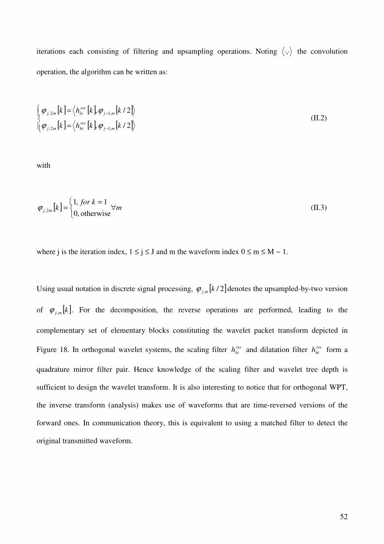
52
iterations each consisting of filtering and upsampling operations. Noting ⋅⋅, the convolution
operation, the algorithm can be written as:
[ ] [ ] [ ]
[ ] [ ] [ ]
=
=
−
−
2/,
2/,
,12,
,12,
kkhk
kkhk
mj
rec
himj
mj
rec
lomj
ϕϕ
ϕϕ (II.2)
with
[ ] mkfor
kmj ∀ =
=otherwise ,0
1 ,12,ϕ (II.3)
where j is the iteration index, 1 ≤ j ≤ J and m the waveform index 0 ≤ m ≤ M − 1.
Using usual notation in discrete signal processing, [ ]2/, kmjϕ denotes the upsampled-by-two version
of [ ]kmj ,ϕ . For the decomposition, the reverse operations are performed, leading to the
complementary set of elementary blocks constituting the wavelet packet transform depicted in
Figure 18. In orthogonal wavelet systems, the scaling filter rec
loh and dilatation filter rec
hih form a
quadrature mirror filter pair. Hence knowledge of the scaling filter and wavelet tree depth is
sufficient to design the wavelet transform. It is also interesting to notice that for orthogonal WPT,
the inverse transform (analysis) makes use of waveforms that are time-reversed versions of the
forward ones. In communication theory, this is equivalent to using a matched filter to detect the
original transmitted waveform.
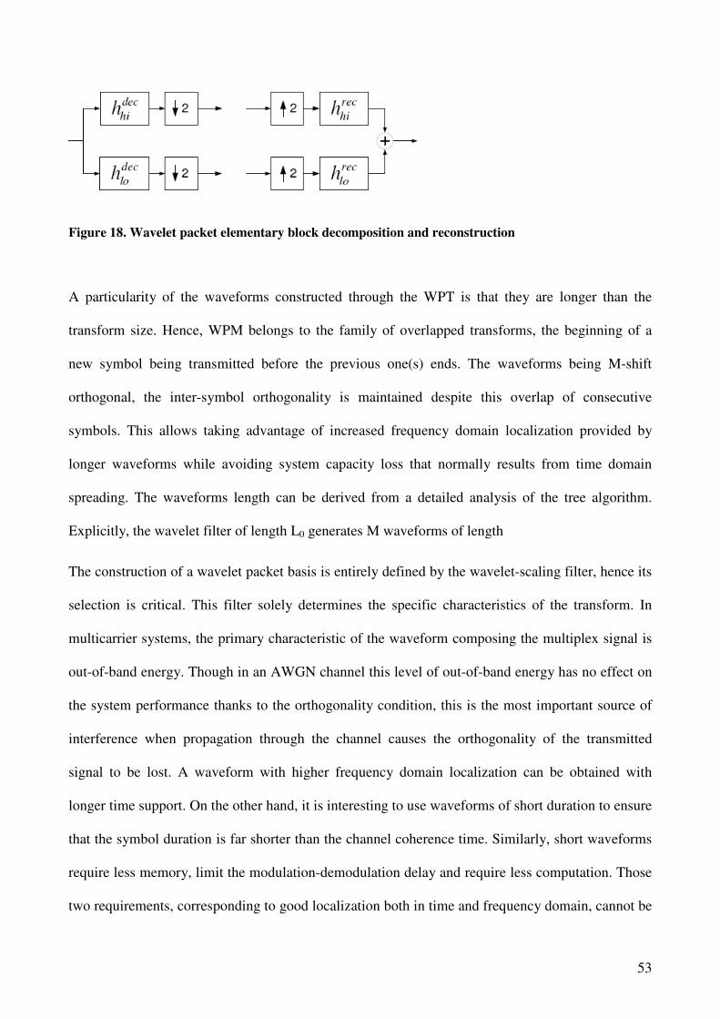
53
Figure 18. Wavelet packet elementary block decomposition and reconstruction
A particularity of the waveforms constructed through the WPT is that they are longer than the
transform size. Hence, WPM belongs to the family of overlapped transforms, the beginning of a
new symbol being transmitted before the previous one(s) ends. The waveforms being M-shift
orthogonal, the inter-symbol orthogonality is maintained despite this overlap of consecutive
symbols. This allows taking advantage of increased frequency domain localization provided by
longer waveforms while avoiding system capacity loss that normally results from time domain
spreading. The waveforms length can be derived from a detailed analysis of the tree algorithm.
Explicitly, the wavelet filter of length L0 generates M waveforms of length
The construction of a wavelet packet basis is entirely defined by the wavelet-scaling filter, hence its
selection is critical. This filter solely determines the specific characteristics of the transform. In
multicarrier systems, the primary characteristic of the waveform composing the multiplex signal is
out-of-band energy. Though in an AWGN channel this level of out-of-band energy has no effect on
the system performance thanks to the orthogonality condition, this is the most important source of
interference when propagation through the channel causes the orthogonality of the transmitted
signal to be lost. A waveform with higher frequency domain localization can be obtained with
longer time support. On the other hand, it is interesting to use waveforms of short duration to ensure
that the symbol duration is far shorter than the channel coherence time. Similarly, short waveforms
require less memory, limit the modulation-demodulation delay and require less computation. Those
two requirements, corresponding to good localization both in time and frequency domain, cannot be

54
chosen independently. In fact, it has been shown that in the case of wavelets, the bandwidth-
duration product is constant. This is usually referred to as the uncertainty principle.
Finally, a minor difference between OFDM and WPM remains to be emphasized. In the former, the
set of waveforms is by nature defined in the complex domain. WPM, on the other hand, is generally
defined in the real domain but can be also defined in the complex domain, solely depending of the
scaling and dilatation filter coefficients. Since the most commonly encountered WPT are defined in
the real domain, it has naturally led the authors to use PAM. It is nevertheless possible to translate
the M real waveform directly in the complex domain. The resulting complex WPT is then
composed of 2M waveforms forming an orthogonal set.

55
Chapter III
Wavelet Filter Bank
3.1 Introduction
A wavelet is a waveform of effectively limited duration that has an average value of zero. Fourier
analysis represents signals as linear combinations of sine and cosine waves, and therefore the
representations are localized in frequency, not in time.
The wavelet analysis uses linear combinations of basis functions (wavelet), localized both in time
and frequency.
f (t) = Linear combination of basis functions (wavelets)
( ) ( )twbtf kj
kj
kj ,
,
,∑= (III.1)
where j and k are dilation (or scale) and translation indices respectively, and wj,k denotes a wavelet
basis which is a collection of functions obtained by dilating and translating a scaling function φ and
a mother wavelet ψ.
By combining the scaling and wavelet functions, we can represent any class of signal as:
( )∑∑∑∞
−∞=
∞
=
∞
−∞=
−+−=k j
j
kj
k
k ktdktctf0
, 2)()( ψφ (III.2)
where the indices j and k are stated as above, and ck and dj,k denote the scaling and details
coefficients respectively.

56
Comparing wavelets with sine waves, which are the basis of Fourier analysis, it has been observed
that sinusoids do not have limited duration, they extend from minus to plus infinity. And where
sinusoids are smooth and predictable, wavelets tend to be irregular and asymmetric.
Signals with sharp changes might be better analyzed with an irregular wavelet than with a smooth
sinusoid.
Wavelet analysis is a windowing technique with variable sized regions. It allows the use of long
time intervals where more precise low-frequency information is required, and shorter regions where
high-frequency information is desired.
Wavelet analysis is capable of revealing aspects of data that other signal analysis techniques miss;
aspects such as trends, breakdown points, discontinuities in higher derivatives, and self similarity.
Furthermore, because it affords a different view of data than those presented by traditional
techniques, wavelet analysis can often compress or denoise a signal without appreciable
degradation.
There exist many different types of wavelet transforms all starting from the basic formulas.
� The continuous wavelet transform (CWT)
� The discrete wavelet transform (DWT)
The distinction among the various types of WT depends on the way in which the scale and shift
parameters are discretized.
3.2 Continuous wavelet transform
For CWT the parameters vary in a continuous fashion. This representation offers the maximum
freedom in the choice of the analysis wavelet. The only requirement is that the wavelet satisfies an
admissibility condition, in particular it must have zero mean. The condition is also crucial to be
CWT invertible on its range. The inverse transform is given by relation (Burrus97):

57
2),(),(
1)(
a
dadbbabaC
Kxf ψ
ψ∫∞
∞−
= (III.3)
and ψ satisfies the admissibility condition:
∞<= ∫∞
∞−
dww
wK
)(ψ̂ψ (III.4)
where ψ̂ is the FT of ψ.
From an intuitive point of view, the CWT consists of calculating a “resemblance index” between
the signal and the wavelet (recall the definition of autocorrelation function).
The continuous wavelet transform is the sum over all time of the signal multiplied by scaled, shifted
versions of the wavelet. This process produces wavelet coefficients that are a function of scale and
position.
The steps of an easy recipe for creating a CWT are (Figure 19):
1) Take a wavelet and compare it to a section at the start of the original signal.
2) Calculate a number, C, that represents how closely correlated the wavelet is with this section
of the signal. The higher C is, the more the similarity. More precisely, if the signal energy
and the wavelet energy are equal to one, C may be interpreted as a correlation coefficient.
(Note that the results will depend on the shape of the wavelet you choose).
3) Shift the wavelet to the right and repeat steps 1 and 2 until you've covered the whole signal.
Choosing scales and positions based on powers of two (so-called dyadic scales and positions) our
analysis will be much more efficient and just as accurate. We obtain such an analysis from the
discrete wavelet transform (DWT). An interesting feature of wavelet analysis is that all of these
time domain signals have the same general shape, and that in fact, they only differ by compressions
and expansions by powers of two.
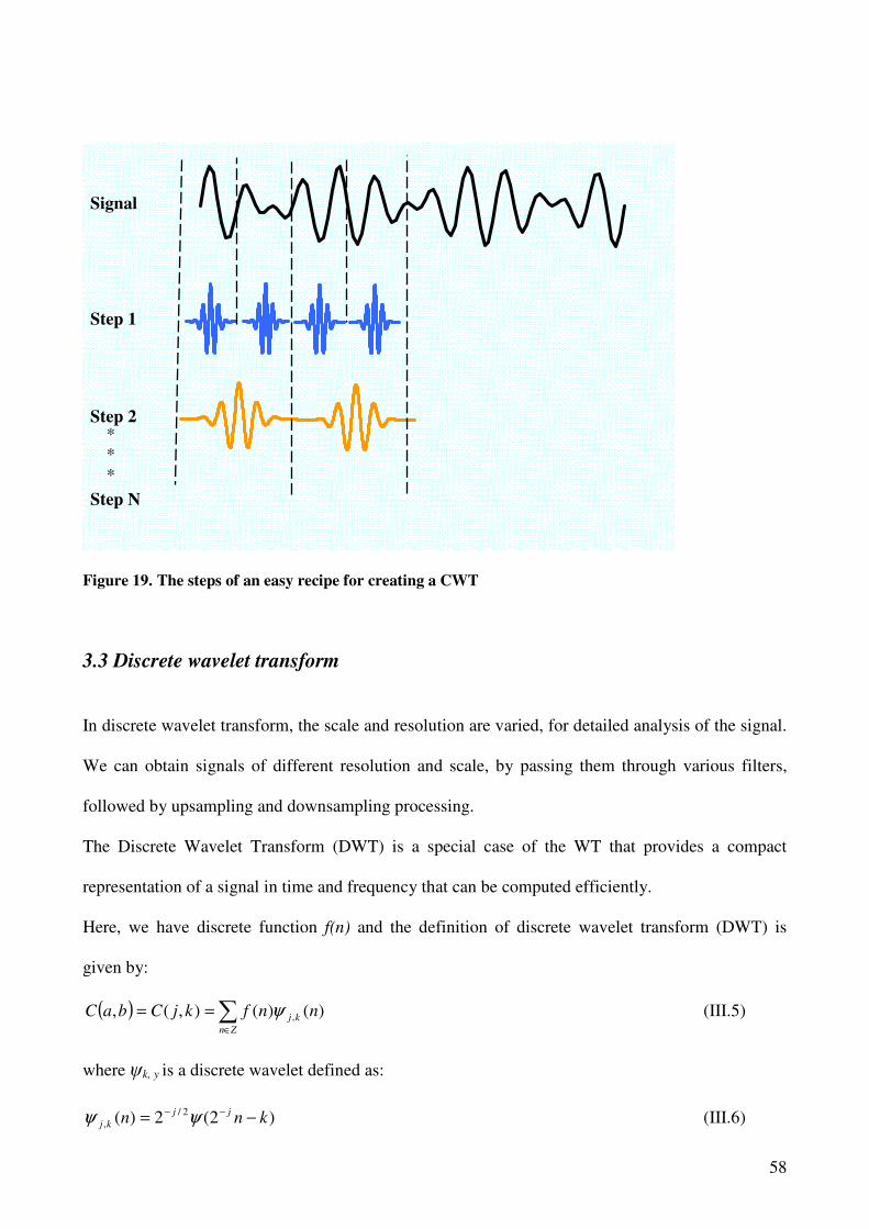
58
Figure 19. The steps of an easy recipe for creating a CWT
3.3 Discrete wavelet transform
In discrete wavelet transform, the scale and resolution are varied, for detailed analysis of the signal.
We can obtain signals of different resolution and scale, by passing them through various filters,
followed by upsampling and downsampling processing.
The Discrete Wavelet Transform (DWT) is a special case of the WT that provides a compact
representation of a signal in time and frequency that can be computed efficiently.
Here, we have discrete function f(n) and the definition of discrete wavelet transform (DWT) is
given by:
( ) ∑∈
==Zn
kj nnfkjCbaC )()(),(, ,ψ (III.5)
where ψk, y is a discrete wavelet defined as:
)2(2)( 2/
, knnjj
kj −= −− ψψ (III.6)
Signal
Step 1
Step 2
Step N
*
*
*

59
The parameters a,b are defined in such a way that a = 2 j ,b = 2
jk. Sometimes the analysis is called
dyadic as well. The inverse transform is defined in a similar way like:
)(),()( , nkjCnf kj
Zj Zk
ψ∑∑∈ ∈
= (III.7)
If the framebounds are such that A=B=1, then the transformation is orthogonal.
Such wavelets can be constructed by starting from a multiresolution analysis that is discussed in
next section.
The DWT is computed by successive lowpass and highpass filtering of the discrete time-domain
signal as shown in Figure 20. This is called the Mallat algorithm or Mallat-tree decomposition. Its
significance is in the manner it connects the continuous-time mutiresolution to discrete-time filters.
In the Figure 20, the signal is denoted by the sequence x[n], where n is an integer.
The low pass filter is denoted by G0 while the high pass filter is denoted by H0. At each level, the
high pass filter produces detail information, d[n], while the low pass filter associated with scaling
function produces coarse approximations, a[n].
At each decomposition level, the half band filters produce signals spanning only half the frequency
band. This doubles the frequency resolution as the uncertainty in frequency is reduced by half. In
accordance with Nyquist’s rule if the original signal has a highest frequency of ω, which requires a
sampling frequency of 2ω radians, then it now has a highest frequency of ω/2 radians. It can now be
sampled at a frequency of ω radians thus discarding half the samples with no loss of information.
This decimation by 2 halves the time resolution as the entire signal is now represented by only half
the number of samples. Thus, while the half band low pass filtering removes half of the frequencies
and thus halves the resolution, the decimation by 2 doubles the scale.
With this approach, the time resolution becomes arbitrarily good at high frequencies, while the
frequency resolution becomes arbitrarily good at low frequencies. The filtering and decimation
process is continued until the desired level is reached. The maximum number of levels depends on

60
the length of the signal. The DWT of the original signal is then obtained by concatenating all the
coefficients, a[n] and d[n], starting from the last level of decomposition.
Figure 20. Wavelet filter bank
Figure 21. Uniform wavelet packet decomposition.
x[n]
LPF
HPF
↓2
↓2
LPF
HPF
↓2
↓2
a’’[n]
d’’[n]
LPF
HPF
↓2
↓2
a’[n]
d’[n]
x[n]
LPF
HPF
↓2
↓2
a[n]
d[n]
G0
H0
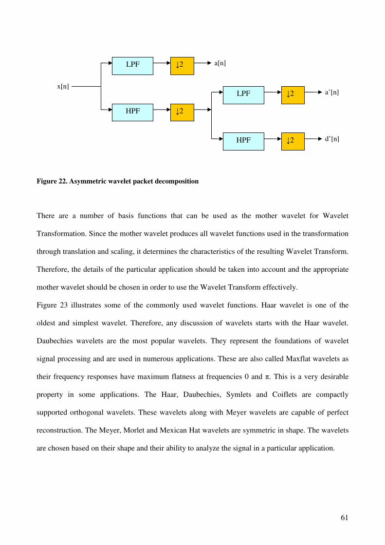
61
Figure 22. Asymmetric wavelet packet decomposition
There are a number of basis functions that can be used as the mother wavelet for Wavelet
Transformation. Since the mother wavelet produces all wavelet functions used in the transformation
through translation and scaling, it determines the characteristics of the resulting Wavelet Transform.
Therefore, the details of the particular application should be taken into account and the appropriate
mother wavelet should be chosen in order to use the Wavelet Transform effectively.
Figure 23 illustrates some of the commonly used wavelet functions. Haar wavelet is one of the
oldest and simplest wavelet. Therefore, any discussion of wavelets starts with the Haar wavelet.
Daubechies wavelets are the most popular wavelets. They represent the foundations of wavelet
signal processing and are used in numerous applications. These are also called Maxflat wavelets as
their frequency responses have maximum flatness at frequencies 0 and π. This is a very desirable
property in some applications. The Haar, Daubechies, Symlets and Coiflets are compactly
supported orthogonal wavelets. These wavelets along with Meyer wavelets are capable of perfect
reconstruction. The Meyer, Morlet and Mexican Hat wavelets are symmetric in shape. The wavelets
are chosen based on their shape and their ability to analyze the signal in a particular application.
x[n]
LPF
HPF
↓2
↓2
a[n]
LPF
HPF
↓2
↓2
a’[n]
d’[n]

62
Figure 23. Wavelet families (a) Haar (b) Daubechies4 (c) Coiflet1 (d) Symlet2 (e) Meyer (f) Morlet (g)
Mexican Hat.
There is a wide range of applications for Wavelet Transforms. They are applied in different fields
ranging from signal processing to biometrics, and the list is still growing. One of the prominent
applications is in the FBI fingerprint compression standard. Wavelet Transforms are used to
compress the fingerprint pictures for storage in their data bank. The previously chosen Discrete
Cosine Transform (DCT) did not perform well at high compression ratios. It produced severe
blocking effects which made it impossible to follow the ridge lines in the fingerprints after
reconstruction. This did not happen with Wavelet Transform due to its property of retaining the
details present in the data.
In DWT, the most prominent information in the signal appears in high amplitudes and the less
prominent information appears in very low amplitudes. Data compression can be achieved by
discarding these low amplitudes. The wavelet transforms enables high compression ratios with good
quality of reconstruction. At present, the application of wavelets for image compression is one the

63
hottest areas of research. Recently, the Wavelet Transforms have been chosen for the JPEG 2000
compression standard.
Wavelets also find application in speech compression, which reduces transmission time in mobile
applications. They are used in denoising, edge detection, feature extraction, speech recognition,
echo cancellation and others. They are very promising for real time audio and video compression
applications. Wavelets also have numerous applications in digital communications. Orthogonal
Frequency Division Multiplexing (OFDM) is one of them. Wavelets are used in biomedical
imaging. For example, the ECG signals, measured from the heart, are analyzed using wavelets or
compressed for storage. The popularity of Wavelet Transform is growing because of its ability to
reduce distortion in the reconstructed signal while retaining all the significant features present in the
signal.

64
Chapter IV
Design of a spectrum sensing system using the Discrete Wavelet
Packet Transformation (DWPT) and WPDM transmission system
This thesis proposes a new method based on the wavelet transformation and its discrete application,
the Discrete Wavelet Packet Transformation (DWPT). We develop a wavelet based method to
efficiently estimate the spectrum and utilize its non-interference zones for secondary users
transmission. We use the wavelet packet decomposition to detect frequency holes through power
estimation of the subbands.
Moreover this method uses a common architecture based on WPDM for transmitting and receiving
signals. WPDM is a multiple signal transmission technique in which the message signals are
waveform coded onto wavelet packet basis functions for transmission. To define the wavelet packet
basis functions we refer to wavelet multiresolution analysis (MRA), the details of which can be
found in a number of textbooks [1]–[2] and tutorial articles [3]–[4].
4.1 Wavelet multiresolution analysis and DWPT
Multiple transmission of heterogeneous services is a central aspect of broadcasting technology.
Often, in this framework, the design of efficient communication systems is complicated by stringent
bandwidth constraint. In wavelet packet division multiplexing (WPDM) the message signals are
waveform coded onto wavelet packet basis functions. The overlapping nature of such waveforms in

65
both time and frequency allows improving the performance over the commonly used FDM and
TDM schemes, while their orthogonality properties permits to extract the message signals by a
simple correlator receiver. Furthermore, the scalable structure of WPDM makes it suitable for
broadcasting heterogeneous services. To define the wavelet packet basis functions we refer to
wavelet multiresolution analysis (WMRA) [2].
Let [ ]ng0 be a unit-energy real causal FIR filter of length N which is orthogonal to its even
translates; i.e., [ ] [ ] [ ]mmngngn
δ=−∑ 200 , where [ ]mδ is the Kroneker delta, and let [ ]ng1 be the
(conjugate) quadrature mirror filter (QMF), [ ] ( ) [ ]1 01 1
ng n g N n= − − − . If [ ]ng0 satisfies some mild
technical conditions [1]-[4], we can use an iterative algorithm to find the function
( ) [ ] ( )01 0 01 02 2n
t g n t nTφ φ= −∑ for an arbitrary interval 0T . Subsequently, we can define the family of
functions lm
φ , 0≥l , lm 21 ≤≤ in the following (binary) tree-structured manner:
( ) [ ] ( )
( ) [ ] ( )1,2 1 0
1,2 1
l m lm ln
l m lm ln
t g n t nT
t g n t nT
φ φ
φ φ
+ −
+
= −
= −
∑∑ (IV.1)
where 02 TT ll = . For any given tree structure, the function at the leafs of the tree form a wavelet
packet.
Wavelet packets have a finite duration, ( )1l
N T− and are self- and mutually-orthogonal at integer
multiples of dyadic intervals.
In WPDM binary messages [ ]lmx n have polar representation (i.e., [ ] 1
lmx n = ± ), waveform coded by
pulse amplitude modulation (PAM) of ( )lm l
t nTφ − and then added together to form the composite
signal ( )s t . WPDM can be implemented using a transmultiplexer and a single modulator [14].
For a two level decomposition
( ) [ ] ( )01 01 0ks t x k t kTφ= −∑ (IV.2)
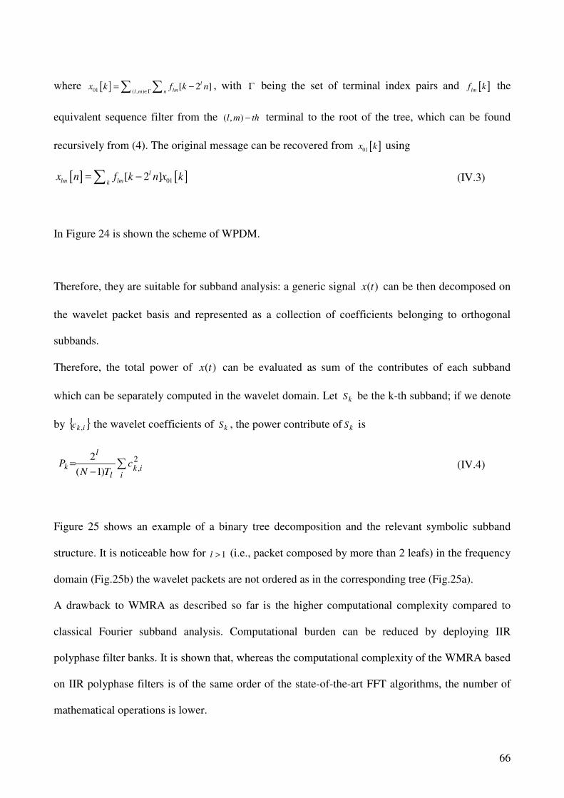
66
where [ ]01 ( , )[ 2 ]
l
lml m nx k f k n
∈Γ= −∑ ∑ , with Γ being the set of terminal index pairs and [ ]lm
f k the
equivalent sequence filter from the ( , )l m th− terminal to the root of the tree, which can be found
recursively from (4). The original message can be recovered from [ ]01x k using
[ ] [ ]01[ 2 ]l
lm lmkx n f k n x k= −∑ (IV.3)
In Figure 24 is shown the scheme of WPDM.
Therefore, they are suitable for subband analysis: a generic signal )(tx can be then decomposed on
the wavelet packet basis and represented as a collection of coefficients belonging to orthogonal
subbands.
Therefore, the total power of )(tx can be evaluated as sum of the contributes of each subband
which can be separately computed in the wavelet domain. Let kS be the k-th subband; if we denote
by { }ikc , the wavelet coefficients of kS , the power contribute of kS is
∑−
=i
ikl
l
k cTN
P2,)1(
2 (IV.4)
Figure 25 shows an example of a binary tree decomposition and the relevant symbolic subband
structure. It is noticeable how for 1>l (i.e., packet composed by more than 2 leafs) in the frequency
domain (Fig.25b) the wavelet packets are not ordered as in the corresponding tree (Fig.25a).
A drawback to WMRA as described so far is the higher computational complexity compared to
classical Fourier subband analysis. Computational burden can be reduced by deploying IIR
polyphase filter banks. It is shown that, whereas the computational complexity of the WMRA based
on IIR polyphase filters is of the same order of the state-of-the-art FFT algorithms, the number of
mathematical operations is lower.

67
01
φ
11φ
12φ
21φ
22φ
31φ
32φ
33φ 34
φ
23φ
24φ
0[ ]g n
1[ ]g n
0[ ]g n
0[ ]g n
0[ ]g n
0[ ]g n
1[ ]g n
1[ ]g n 1
[ ]g n
(a)
f
31φ
32φ
33φ
34φ
23φ 24
φ
Bw / 2Bw
/ 4Bw
/ 8Bw
(b)
Figure 25. (a) Wavelet tree structure (b) Corresponding symbolic subband structure.
0[ ]g i− 0[ ]g i
1[ ]g i
0[ ]g i
1[ ]g i 1[ ]g i−
1[ ]g i−
0[ ]g i− 2
2
2
2
2
2
2
2
21[ ]x n
( )01 0t kTφ −
22[ ]x n
23[ ]x n
24[ ]x n
Channel
$21[ ]x n
$22[ ]x n
$23[ ]x n
$24[ ]x n
Matched
Filter
01( )tφ −
01[ ]x k
01ˆ [ ]x k
2
0T KT=2
2
0[ ]g i
1[ ]g i
2
2
0[ ]g i−
1[ ]g i−
( )s t ( )r t
Level 1 Level 2
Figure 24. Transmitter and receiver for two level WPDM system.

68
4.2 Spectrum Sensing Algorithms
4.2.1 Power Analysis
The sensing of spectrum is accomplished in according to the following algorithm, briefly sketched
in Figure 26.
Its goal is to automatically define a feature set to identify spectrum opportunities or holes.
The main tasks of the sensing process are:
1) Performing a wavelet decomposition of the signal to obtain a plurality of wavelet coefficients
into a plurality of subbands.
2) Computing the power of each channel.
3) For each subband, verifying if the calculated power is less than a fixed power threshold.
4) Identification of white spaces.
For each subband P > Thp
Mark the band as being free
Discard the subband
N Y
List of free subbands
(white spaces)
SPECTRUM
Figure 26. Spectrum sensing algorithm based on power estimation
We calculate the power of the signal according to [1], as explained in the following section.
If a received signal, s(t) is periodic signal with period T, then, the power of this signal is computed
by
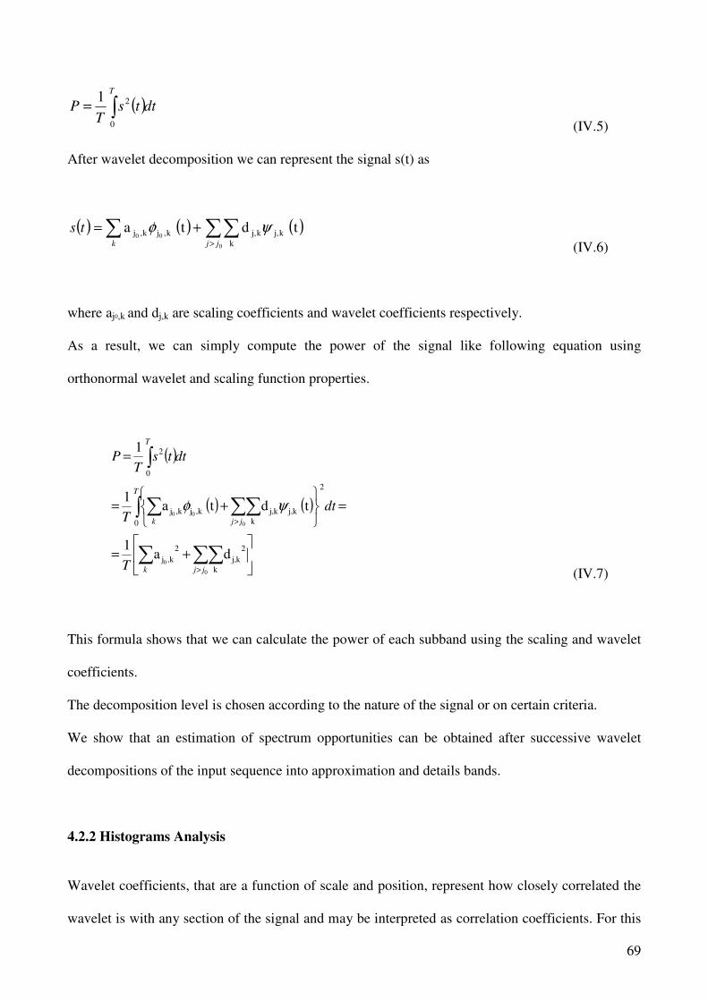
69
( )dttsT
P
T
∫=0
21
(IV.5)
After wavelet decomposition we can represent the signal s(t) as
( ) ( ) ( )∑∑∑>
+=0
00
k
kj,kj,k,jk,j t dt ajjk
ts ψφ
(IV.6)
where aj0,k and dj,k are scaling coefficients and wavelet coefficients respectively.
As a result, we can simply compute the power of the signal like following equation using
orthonormal wavelet and scaling function properties.
( )
( ) ( )
+=
=
+=
=
∑∑∑
∫ ∑∑∑
∫
>
>
0
0
0
00
k
2
kj,
2
k,j
2
0 k
kj,kj,k,jk,j
0
2
da1
t dt a1
1
jjk
T
jjk
T
T
dtT
dttsT
P
ψφ
(IV.7)
This formula shows that we can calculate the power of each subband using the scaling and wavelet
coefficients.
The decomposition level is chosen according to the nature of the signal or on certain criteria.
We show that an estimation of spectrum opportunities can be obtained after successive wavelet
decompositions of the input sequence into approximation and details bands.
4.2.2 Histograms Analysis
Wavelet coefficients, that are a function of scale and position, represent how closely correlated the
wavelet is with any section of the signal and may be interpreted as correlation coefficients. For this

70
reason the distribution of coefficients over different values may give us information about the
presence or not of the signal in a subband of the spectrum.
To study the spectrum occupancy we form histograms of coefficients for different subbands.
The following algorithm for automatically forming a feature set to identify spectrum opportunities
or holes, comprises: (a) performing a wavelet decomposition of the signal to obtain a plurality of
wavelet coefficients in a plurality of subbands; (b) forming a histogram of the wavelet coefficients
in each subband; (c) if the value of the coefficients for a determined portion of spectrum tend to
zero so less the wavelet is correlated to the signal. It means that in this subband is a hole (Figure
30); (d) if instead the coefficients are distributed over different values (Figure 31), it needs to
subsequently decompose the signal. A scheme of the proposed algorithm in shown in the next figure
(Figure 27).
Figure 27. Spectrum sensing algorithm based on histogram analysis
Wavelet decomposition
Histogram of coefficients for each
subband
All coefficients
=0
Spectrum hole
yes
no
Vector of coefficients for each subband
Frequency description
of the subbands

71
Let Bn be the n-th subband; we denote by zjn the wavelet coefficients of a Bn. Plotting the histogram
of zjn we obtain the distribution of wavelet coefficient p
n(z).
We can distinguish two possible situations:
a) If the 95% of coefficient is assembled in zero, but there is also another peak in the histogram
we have to decide if the peak is a noise or interference. We define a threshold value T that
plays an essential role. We define T as the ratio between the nonzero coefficient where the
peak is located and the total range of coefficient in this subband: n
n
j
Z
zT = . If T<Th we can
consider the peak as a noise and stop the decomposition process for this subband. T is a
global threshold to be applied to all nonzero wavelet coefficient at different scales. Th is
chosen according to the signal, channel conditions and SNR.
b) If few nonzero wavelet coefficients are located in the neighbourhood of zero we can suppose
a Gaussian distribution. In p n
(z), starting from the maximum and moving to the tails of the
distribution two thresholds are identified, that are: nn aa 21 , . If ( )
= ∑∫
max
min
2
1
95,0 n
j
a
a
n zdxxp and
the ratio of the range between these values and the total range of coefficient in this subband
is less than a constant value the decomposition process can be stopped. These thresholds
identify the wavelet coefficients constituting the critic zone for Bn, that is:
{ } [ ]{ }nnn
j
cr
n aazzzB 21 ,, ∉∈∀= . In other words, a critic zone is composed by those
coefficients located on the distribution's tails identified by the above thresholds.
4.2.3 Simulation results
This section reports some simulation results in order to illustrate the behaviour of our algorithm
based on histograms analysis.
Two distinct cases with different centre frequency and SNR were considered.
Case 1: Figure 28 shows a generic signal using the FFT scheme.

72
Figure 28. Spectrum of a generic signal
Performing a 4-level DWPT (or RI = 4) we obtain 16 channels of 200 kHz.
For simplicity we put indexes to channels in the ascending order.
SPECTRUM
1 2 3 4 5 6 7 8 9 10 11 12 13 14 15 16
Figure 29. Separation of the input bandwidth in 16 subbands using 4-level DWPT

73
From the wavelet decomposition of the signal we have obtained a plurality of wavelet coefficients
in 16 subbands (Figure 29). We have used this set of data to obtain the histograms of subbands. For
the Channel 15 we obtained the Histogram in Figure 30.
Figure 30. Sub-channel 15: a histogram of a free subband
Most of wavelet coefficients for this part of spectrum are zero. It means that in this subband is a
hole.
For the Channel 3 we obtained the Histogram in Figure 31. The coefficients are distributed over
different values. It means that in this subband is the signal.

74
Figure 31. Sub-channel 3: a histogram of an occupied subband
Case 2: Figure 32 shows a generic signal at a CPE using the FFT scheme
Figure 32. A generic signal at a CPE

75
Performing a 4-level DWPT (or RI = 4) we obtain 16 channels as before
For the Channel 6 we obtained the Histogram in Figure 33.
Figure 33. Sub-channel 6: a histogram of a free subband
For the Channel 3 we obtained the Histogram in Figure 34.
Figure 34. Sub-channel 3: a histogram of an occupied subband
76
Using the scaling and wavelet coefficients we calculated the power for each channel and resulted
that the channels 3, 8, 16 being significantly bigger than the others with respect to the algorithm
presented in 4.2.1.
4.3 Transmitting and receiving data
4.3.1 System Architecture
The architecture for the transmission using the WPM techniques is presented in figure 35
(transmitting) and 36 (receiving) as structured in the simulation built with Simulink. The system is
basically divided into the Wavelet Packet reconstruction block and the PAM Modulation block. In
the particular case of the simulation, the block is a wavelet filter bank on two levels, using
Daubechies filters.
The PAM Modulation block is responsible for modulating the multiplexed signal using as an
impulse function one of the Daubechies scale functions. The modulator is implemented with a FIR
having a certain interpolation coefficient.
The simulated architecture has, for test purposes, also a Bernoulli binary generator for pseudo-
random binary sequences, which are used for modulating the input channel in the Binary Phase
Shift Keying (BPSK) module.
The same blocks having the inverse function are present also in the architecture of the receiver
(Figure 36).

77
Figure 35. Architecture of the transmission system using WPM technology
Figure 36. Architecture of the receiver using WPM technology

78
A detailed description of the building blocks of the transmitting and receiving architecture, together
with the specific parameters, is presented at the end of this chapter.
4.3.2 Simulation results and performance tests
In the next section are presented results of the performance of WPM in diverse propagation
channels.
Tests proposed in [6] lead us to conclude that this new modulation scheme is a viable alternative to
OFDM to be considered for today’s communication systems.
BER – without channel equalization
In this paragraph we present on comparative results between WPM and OFDM schemes without
channel equalization. While the absence of equalization in a real system would yield a poor
performance in most channels, it is nevertheless of interest to consider this case. The main
motivation is to gain insight on the distortion caused by a given channel to the different modulated
signals. Moreover, since optimal equalization schemes for both are different, the definition of
equivalence between systems would require the choice of appropriate comparison criteria.
With the same concern of comparing equivalent systems, the OFDM reference system used in this
section has no cyclic prefix. The addition of a prefix is indeed a technique aiming at rendering the
multipath distortion easier to cancel and as such can be considered as a form of equalization. Since
no similar artefact is available for WPM, the comparison is fairer if no cyclic prefix is used. In
addition, the introduction of the cyclic prefix leads to a bandwidth efficiency loss and thus this
would add to the difference between modulation schemes.
We choose to assume here the simple case of a time invariant 2-path channel model. The first path
has unit power and the second path power is 3 dB lower. The relative delay of the second path τ is
a simulation parameter. The BER versus the second path delayτ curves of WPM(db2), WPM(db6),
and WPM(db10) schemes with 32 QPSK modulated subcarriers is shown in Figure 37. All curves
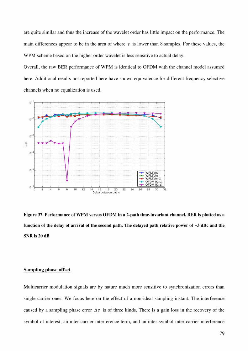
79
are quite similar and thus the increase of the wavelet order has little impact on the performance. The
main differences appear to be in the area of where τ is lower than 8 samples. For these values, the
WPM scheme based on the higher order wavelet is less sensitive to actual delay.
Overall, the raw BER performance of WPM is identical to OFDM with the channel model assumed
here. Additional results not reported here have shown equivalence for different frequency selective
channels when no equalization is used.
Figure 37. Performance of WPM versus OFDM in a 2-path time-invariant channel. BER is plotted as a
function of the delay of arrival of the second path. The delayed path relative power of −3 dBc and the
SNR is 20 dB
Sampling phase offset
Multicarrier modulation signals are by nature much more sensitive to synchronization errors than
single carrier ones. We focus here on the effect of a non-ideal sampling instant. The interference
caused by a sampling phase error τ∆ is of three kinds. There is a gain loss in the recovery of the
symbol of interest, an inter-carrier interference term, and an inter-symbol inter-carrier interference

80
contribution. This last term originates from the symbol overlapping and thus does not exist in
OFDM. Hence, the sensitivity of WPM is expected to be higher than for OFDM. In addition, the
BER degradation depends on the auto-correlation of each subcarrier waveform, which differs
between subcarriers. Overall, the BER of the multicarrier signal can be obtained as the average of
the BER over each individual subcarrier. Since no analytical closed form solution is available, the
sensitivity of each modulation scheme to sampling instant error has been obtained by simulation.
Figure 38 reports link BER as a function of the sampling phase offset normalized to the sampling
period. For this particular simulation, the channel is modelled as AWGN with 20 dB SNR. As it
was expected due to the overlapping of symbols, WPM is more sensitive than OFDM to an
imperfect sampling instant. A BER of 10−4 is achieved for OFDM at a normalized sampling error
of 27%, while WPM(db2) requires less than 21%. For the two other WPM schemes, the error
tolerated is slightly lower, with a maximum of about 18%.
Figure 38. Sensitivity of different WPM schemes versus OFDM schemes to sampling phase error,
expressed as the link BER versus the normalized sampling phase error.

81
Presence of a narrow band interferer
With today’s growing use of wireless systems, the radio-frequency spectrum is becoming more and
more congested by communication signals. In such a condition, future modulation schemes have to
cope not only with channel distortion, but also with interference originating from other sources as
well. Moreover, multicarrier modulation is very likely to encounter in-band interfering signal since
it is usually best suited for wideband communication systems.
We assume the case of a WPM link communication over an AWGN channel and exposed to an in-
band, unmodulated signal superimposed on the signal of interest at the receiver. We denote Pdist as
the power of the disturbing signal and fdist as its frequency. The amount of interference endowed by
each subcarrier k can thus be approximated as
∑−
=
Φ=1
0
2)(
M
k
distkdistI fPP (IV.8)
where kΦ is the Fourier transform of kϕ . In the case of waveforms with null out-of-band energy,
the disturbance will be limited to the subcarrier whose band includes the frequency fdist. With an
actual system, additional disturbance is caused by the side lobes of the adjacent subcarriers. The
side lobe energy level decreasing with the order of the wavelet, the sensitivity of WPM to a single
tone disturber can thus be reduced by increasing the order of the generating wavelet. Results
obtained through simulation are shown in Figure 39, where the BER performance of WPM(db2),
WPM(db8), and OFDM links are plotted as a function of the disturber normalized frequency Fdist.

82
Figure 39. Link BER in the presence of a single tone disturber as a function of the disturber
frequency, for WPM(coif1), WPM(coif5), WPM(dmey), and OFDM schemes.
A 16-subcarrier scheme with 16QAM-modulated symbols has been chosen to point out the effect of
the disturber. The disturber has power equal to the signal of interest, i.e. Pdist = 0 dBc. The curves
obtained for all modulation schemes show clearly that the level of interference is highly dependent
on the actual disturber frequency. Hence, the curve for OFDM shows clearly the higher BER when
the disturber frequency corresponds to the centre frequency of one subcarrier. The WPM schemes
show a similar effect but with a smoother curve. Considering the average over the whole frequency
band, WPM(coif5) and WPM(dmey) outperform OFDM. The WPM(coif1) scheme however shows
more degradation than OFDM.
Overall, the WPM schemes seem to be able to perform better than OFDM when a wavelet with
sufficiently low out-of-band energy is used. For a given wavelet, there appear to be a gain in
robustness with the increase in generating wavelet order. Additional results are presented in Figure
40 where the link BER of the same schemes as previously are given as a function of the disturber

83
relative power Pdist. Its normalized frequency has been arbitrary chosen to be 0.1666, which can be
verified from the previous figure to correspond to the case where WPM leads to an average gain in
comparison with OFDM. The WPM(coif1) scheme performs overall quite similarly to OFDM, but
with a robustness to disturber about 2 dB lower. The WPM(coif5) and WPM(dmey) schemes, on
the other hand, provide a much higher robustness than OFDM for a disturber power of up to -15 dB.
Past this threshold, it is noticeable that OFDM has instead a lower sensitivity, being undisturbed for
Pdist lower than −20dB while the two WPM schemes require about 2 dB less.
Figure 40. Link BER in the presence of a single tone disturber as a function of the disturber power, for
WPM(coif1), WPM(coif5), WPM(dmey), and OFDM schemes.
In general, the degradation in terms of BER of the WPM signal due to a single tone disturber is
highly dependent on both its frequency and power. The results obtained have nevertheless shown
that WPM schemes are capable of high immunity to disturbance when higher order wavelets are
selected.

84
4.4 Possible schemes of simulation and different configuration of the system
4.4.1 Communication based on a Coordinator
- communication architecture based on a local coordinator which broadcasts information
about free bands.
- the secondary users (SU) implement the same TX / RX WPDM -based blocks
- the SU don’t exchange spectrum occupation data among them
- the communication between coordinator and SU is unidirectional (coordinator broadcasts)
Figure 41. Configuration based on a coordinator
Parameters:
B – bandwidth = 200 kHz, Tp – power treshold = - 90 dBm
Secondary user:
- receives the broadcast from the coordinator which senses e.g. the first 32 channels of the
uplink P-GSM band (890 – 896.4 MHz )
- decodes the wavelet coefficients and reconstructs the wavelet tree
- calculates power in every subband and compares it with the Tp parameter
- validates the subbands (coloured once are detected as being free)
COORDINATOR
SECONDARY
USER 1
SECONDARY
USER 2
SECONDARY
USER 3
B1,Tn1
B2,Tn2
B3,Tn3

85
- the required bandwidth is 200 kHz therefore we look for two adjacent 100 MHz subbands
belonging to the same tree since the resulting subbands of the WPDM are not ordered in
frequency
- 1,2 and 29,30 match the criteria whereas 6,7 and 16,17 do not belong to the same tree
- based on the preferred band parameter, the SU begins transmission on the 1+2 subbands
- the algorithm is repeated after a certain amount of time based on the updated information
received by the coordinator. If the resulted free bands do not match with the current
situation the transmission is halted or moved to another subband if available or more
convenient.
Figure 42. Spectrum sensing using WPDM with e.g. 5 levels.
4.4.2 Communication without a Coordinator
The communication architecture between Secondary Users (SU) is based on local spectrum sensing
implemented by each SU, completed with communication (TX/RX), all based on WPDM
technology. The communication is direct, without the aid of a controller or supervisor.
Each SU performs its on spectrum sensing based on the above presented algorithm on 32 subbands
(Figure 42) and is afterwards in possession of a list with the spectrum holes suitable for
transmission. The SU who wants to initiate the communication, sends its own and the peers’ MAC
address as a broadcast on all frequencies found free. If the peer succeeds to receive the two MAC
addresses on one or more frequencies, he sends back, together with the same MACs his list of
1 2 3 4 5 6 7 8 9 10 11 12 13 14 15 16 17 18 19 20 21 22 23 24 25 26 27 28 29 30 31 32

86
available spectrum holes. The initiator receives the data and decides on which frequency
(frequencies) to transmit the actual data. Next figures illustrate the communication sequence.
- broadcast of the own MAC and the MAC of the peer in the white spaces
- wait for an answer from the peer (SU2)
Figure 43. Communication sequence between two secondary users: Step 1
- the peer has performed previously its own sensing and decides based on sensing and
incoming data which bands will be used
SECONDARY
USER 1
SECONDARY
USER 2
1
16
2
17
29
30
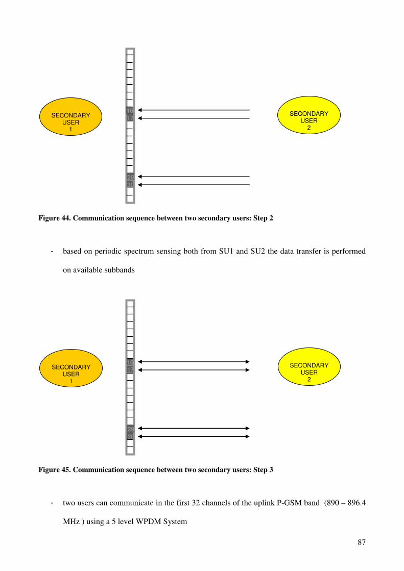
87
Figure 44. Communication sequence between two secondary users: Step 2
- based on periodic spectrum sensing both from SU1 and SU2 the data transfer is performed
on available subbands
Figure 45. Communication sequence between two secondary users: Step 3
- two users can communicate in the first 32 channels of the uplink P-GSM band (890 – 896.4
MHz ) using a 5 level WPDM System
SECONDARY
USER 1
SECONDARY
USER 2
16 17
29
30
SECONDARY
USER 1
SECONDARY
USER 2
16 17
29
30
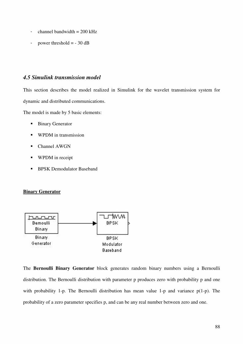
88
- channel bandwidth = 200 kHz
- power threshold = - 30 dB
4.5 Simulink transmission model
This section describes the model realized in Simulink for the wavelet transmission system for
dynamic and distributed communications.
The model is made by 5 basic elements:
� Binary Generator
� WPDM in transmission
� Channel AWGN
� WPDM in receipt
� BPSK Demodulator Baseband
Binary Generator
The Bernoulli Binary Generator block generates random binary numbers using a Bernoulli
distribution. The Bernoulli distribution with parameter p produces zero with probability p and one
with probability 1-p. The Bernoulli distribution has mean value 1-p and variance p(1-p). The
probability of a zero parameter specifies p, and can be any real number between zero and one.

89
The BPSK Modulator Baseband block modulates using the binary phase shift keying method. The
output is a baseband representation of the modulated signal. For both integer and bit inputs, this
block can accept the data types int8, uint8, int16, uint16, int32, uint32, boolean, single, and double.
The input must be a discrete-time binary-valued signal. If the input bit is 0 or 1, respectively, then
the modulated symbol is exp(jθ) or -exp(jθ) respectively, where θ is the Phase offset parameter.

90
WPDM in transmission
The Wavelet Packet Reconstruction block reconstructs a signal from its subbands with smaller
bandwidths and slower sample rates. Uses a filter bank with specified low-pass and high-pass FIR
filters, which can be user-defined or wavelet-base. Usually, the low-pass and high-pass filters
should be half-band filters designed to complement each other.
The reconstructed signal has a wider bandwidth and faster sample rate than the input subbands.

91
The FIR Interpolation block resamples the discrete-time input at a rate L times faster than the input
sample rate, where the integer L is specified by the Interpolation factor parameter. This process
consists of two steps:
� The block upsamples the input to a higher rate by inserting L-1 zeros between samples.
� The block filters the upsampled data with a direct-form FIR filter.
AWGN Channel
The AWGN Channel block adds white Gaussian noise to a real or complex input signal. When the
input signal is real, this block adds real Gaussian noise and produces a real output signal. When the
input signal is complex, this block adds complex Gaussian noise and produces a complex output
signal.
This block inherits its sample time from the input signal.
WPDM in receipt
This part is made by 3 blocks:
� Digital Filter
� Downsample
� Wavelet Packet Decomposition
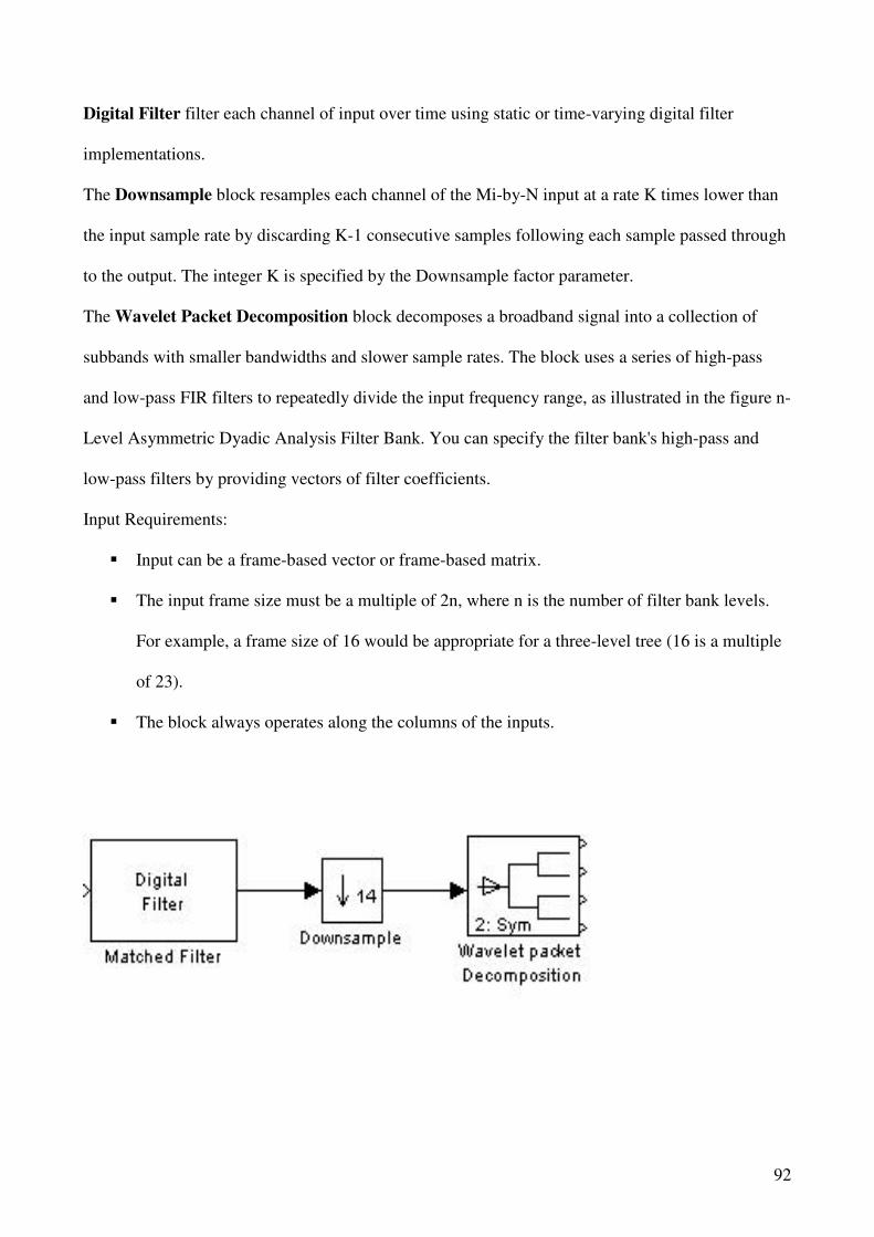
92
Digital Filter filter each channel of input over time using static or time-varying digital filter
implementations.
The Downsample block resamples each channel of the Mi-by-N input at a rate K times lower than
the input sample rate by discarding K-1 consecutive samples following each sample passed through
to the output. The integer K is specified by the Downsample factor parameter.
The Wavelet Packet Decomposition block decomposes a broadband signal into a collection of
subbands with smaller bandwidths and slower sample rates. The block uses a series of high-pass
and low-pass FIR filters to repeatedly divide the input frequency range, as illustrated in the figure n-
Level Asymmetric Dyadic Analysis Filter Bank. You can specify the filter bank's high-pass and
low-pass filters by providing vectors of filter coefficients.
Input Requirements:
� Input can be a frame-based vector or frame-based matrix.
� The input frame size must be a multiple of 2n, where n is the number of filter bank levels.
For example, a frame size of 16 would be appropriate for a three-level tree (16 is a multiple
of 23).
� The block always operates along the columns of the inputs.

93
BPSK Demodulator Baseband
BPSK Block demodulate BPSK-modulated data
The BPSK Demodulator Baseband block demodulates a signal that was modulated using the binary
phase shift keying method. The input is a baseband representation of the modulated signal. The
input can be either a scalar or a frame-based column vector. The block can accept the data types
single and double. The input must be a discrete-time complex signal. The block maps the points
exp(jθ) and -exp(jθ) to 0 and 1, respectively, where θ is the Phase offset parameter.
94
The model has also secondary blocks:
� Scatter Plot
� Error Rate
� Find Delay
Scatter Plot
The Discrete-Time Scatter Plot Scope block displays scatter plots of a modulated signal, to reveal
the modulation characteristics, such as pulse shaping or channel distortions of the signal. The
Discrete-Time Scatter Plot Scope block has one input port. The input signal must be complex. The
input signal must be complex. The block accepts signal of type double, single, base integer, and
fixed-point for input, but will cast it as double. The input signal must be a sample-based scalar in
sample-based mode. The input must be a frame-based column vector or a scalar in frame-based
mode.

95
Error Rate Calculation
The Error Rate Calculation block compares input data from a transmitter with input data from a
receiver. It calculates the error rate as a running statistic, by dividing the total number of unequal
pairs of data elements by the total number of input data elements from one source.
Find Delay
The Find Delay block finds the delay between a signal and a delayed, and possibly distorted,
version of itself. The block is particularly useful when you want to compare a transmitted and
received signal to find the bit error rate, but do not know the delay in the received signal.

96
97
Chapter V
A case of study: “A cognitive radio system for home
theatre 5+1 audio surround applications”
5.1 AC-3
The United States Advanced Television Systems Committee (ATSC), Inc., was formed by the
member organizations of the Joint Committee on InterSociety Coordination (JCIC)1, recognizing
that the prompt, efficient and effective development of a coordinated set of national standards is
essential to the future development of domestic television services.
One of the activities of the ATSC is exploring the need for and, where appropriate, coordinating the
development of voluntary national technical standards for Advanced Television Systems (ATV).
The ATSC Executive Committee assigned the work of documenting the U.S. ATV standard to a
number of specialist groups working under the Technology Group on Distribution (T3). The Audio
Specialist Group (T3/S7) was charged with documenting the ATV audio standard.
This document was prepared initially by the Audio Specialist Group as part of its efforts to
document the United States Advanced Television Broadcast Standard. It was approved by the
Technology Group on Distribution on 26 September 1994, and by the full ATSC membership as an
ATSC Standard on 10 November 1994. Annex A, “AC-3 Elementary Streams in an MPEG-2
Multiplex,” was approved by the Technology Group on Distribution on 23 February 1995, and by
the full ATSC membership on 12 April 1995. Annex B, “AC-3 Data Stream in IEC958 Interface,”
and Annex C, “AC-3 Karaoke Mode,” were approved by the Technology Group on Distribution on
24 October 1995 and by the full ATSC Membership on 20 December 1995.
98
Revision A of this standard was approved by the full ATSC membership on 20 August 2001.
Revision A corrected some errata in the detailed specifications, revised Annex A to include
additional information about the DVB standard, removed Annex B that described an interface
specification (superseeded by IEC and SMPTE standards), and added a new annex, “Alternate Bit
Stream Syntax,” which contributes (in a compatible fashion) some new features to the AC-3 bit
stream.
Revision B of this standard was approved by the full ATSC membership on 14 June 2005. Revision
B corrected some errata in the detailed specifications, and added a new annex, “Enhanced AC-3 Bit
Stream Syntax” which specifies a non-backwards compatible syntax that offers additional coding
tools and features. Informative references were removed from the body of the document and placed
in a new Annex B.
ATSC Standard A/53C, “Digital Television Standard”, references this document and describes
how the audio coding algorithm described herein is applied in the ATSC DTV standard. The ETSI
TR 101 154 document describes how AC-3 is applied in the DVB DTV standard.
In order to more efficiently broadcast or record audio signals, the amount of information required to
represent the audio signals may be reduced. In the case of digital audio signals, the amount of
digital information needed to accurately reproduce the original pulse code modulation (PCM)
samples may be reduced by applying a digital compression algorithm, resulting in a digitally
compressed representation of the original signal. (The term compression used in this context means
the compression of the amount of digital information which must be stored or recorded, and not the
compression of dynamic range of the audio signal.) The goal of the digital compression algorithm is
to produce a digital representation of an audio signal which, when decoded and reproduced, sounds
the same as the original signal, while using a minimum of digital information (bit-rate) for the
compressed (or encoded) representation. The AC-3 digital compression algorithm specified in this
document can encode from 1 to 5.1 channels of source audio from a PCM representation into a
serial bit stream at data rates ranging from 32 kbps to 640 kbps. The 0.1 channel refers to a

99
fractional bandwidth channel intended to convey only low frequency (subwoofer) signals. A typical
application of the algorithm is shown in Figure 46. In this example, a 5.1 channel audio program is
converted from a PCM representation requiring more than 5 Mbps (6 channels × 48 kHz × 18 bits =
5.184 Mbps) into a 384 kbps serial bit stream by the AC-3 encoder. Satellite transmission
equipment converts this bit stream to an RF transmission which is directed to a satellite
transponder. The amount of bandwidth and power required by the transmission has been reduced by
more than a factor of 13 by the AC-3 digital compression. The signal received from the satellite is
demodulated back into the 384 kbps serial bit stream, and decoded by the AC-3 decoder. The result
is the original 5.1 channel audio program. Digital compression of audio is useful wherever there is
an economic benefit to be obtained by reducing the amount of digital information required to
represent the audio. Typical applications are in satellite or terrestrial audio broadcasting, delivery of
audio over metallic or optical cables, or storage of audio on magnetic, optical, semiconductor, or
other storage media.
Figure 46. Example application of AC-3 to satellite audio transmission.
100
5.1.1 Encoding
The AC-3 encoder accepts PCM audio and produces an encoded bit stream consistent with this
standard. The specifics of the audio encoding process are not normative requirements of this
standard.
The encoding process is briefly described below.
The AC-3 algorithm achieves high coding gain (the ratio of the input bit-rate to the output bitrate)
by coarsely quantizing a frequency domain representation of the audio signal. A block diagram of
this process is shown in Figure 47. The first step in the encoding process is to transform the
representation of audio from a sequence of PCM time samples into a sequence of blocks of
frequency coefficients. This is done in the analysis filter bank. Overlapping blocks of 512 time
samples are multiplied by a time window and transformed into the frequency domain. Due to the
overlapping blocks, each PCM input sample is represented in two sequential transformed blocks.
The frequency domain representation may then be decimated by a factor of two so that each block
contains 256 frequency coefficients. The individual frequency coefficients are represented in binary
exponential notation as a binary exponent and a mantissa. The set of exponents is encoded into a
coarse representation of the signal spectrum which is referred to as the spectral envelope. This
spectral envelope is used by the core bit allocation routine, which determines how many bits to use
to encode each individual mantissa. The spectral envelope and the coarsely quantized mantissas for
six audio blocks (1536 audio samples per channel) are formatted into an AC-3 frame. The AC-3 bit
stream is a sequence of AC-3 frames.
The actual AC-3 encoder is more complex than indicated in Figure 1.2.
The following functions not shown above are also included:
1. A frame header is attached which contains information (bit-rate, sample rate, number of encoded
channels, etc.) required to synchronize to and decode the encoded bit stream.
2. Error detection codes are inserted in order to allow the decoder to verify that a received frame of
data is error free.

101
3. The analysis filterbank spectral resolution may be dynamically altered so as to better match the
time/frequency characteristic of each audio block.
4. The spectral envelope may be encoded with variable time/frequency resolution.
5. A more complex bit allocation may be performed, and parameters of the core bit allocation
routine modified so as to produce a more optimum bit allocation.
6. The channels may be coupled together at high frequencies in order to achieve higher coding gain
for operation at lower bit-rates.
7. In the two-channel mode, a rematrixing process may be selectively performed in order to provide
additional coding gain, and to allow improved results to be obtained in the event that the two-
channel signal is decoded with a matrix surround decoder.
Figure 47. The AC-3 encoder
5.1.2 Decoding
The decoding process is basically the inverse of the encoding process. The decoder, shown in
Figure 48, must synchronize to the encoded bit stream, check for errors, and de-format the various
types of data such as the encoded spectral envelope and the quantized mantissas. The bit allocation
Analysis
Filter Bank
Spectral
Envelope
Encoding
Mantissa
Quantization
AC-3 Frame Formatting
Bit
Allocation
PCM Time
Samples
Exponents
Mantissas
Quantized
Mantissas
Encoded
Spectral
Envelope
Bit Allocation Information

102
routine is run and the results used to unpack and de-quantize the mantissas. The spectral envelope is
decoded to produce the exponents. The exponents and mantissas are transformed back into the time
domain to produce the decoded PCM time samples.
The actual AC-3 decoder is more complex than indicated in Figure 1.3. The following functions not
shown above are included:
1) Error concealment or muting may be applied in case a data error is detected.
2) Channels which have had their high-frequency content coupled together must be de-coupled.
3) Dematrixing must be applied (in the 2-channel mode) whenever the channels have been
rematrixed.
4) The synthesis filterbank resolution must be dynamically altered in the same manner as the
encoder analysis filter bank had been during the encoding process.
The use of a band of spectrum by one system in the vicinity of a second system’s receiver (tuned to
the same band) will generally degrade the performance of that second system if the total
interference exceeds a critical value.
Spectral
Envelope
Decoding
Bit
Allocation
Synthesis
Filter Bank
PCM Time
Samples
Exponents
Mantissas
Quantized
Mantissas Encoded
Spectral
Envelope
Bit Allocation
Information
AC-3 Frame Synchronization, Error Detection
and Frame De-formatting
Mantissa
De-quantization
Encoded AC-
3 Bit-Stream
Figure 48. The AC-3 decoder.
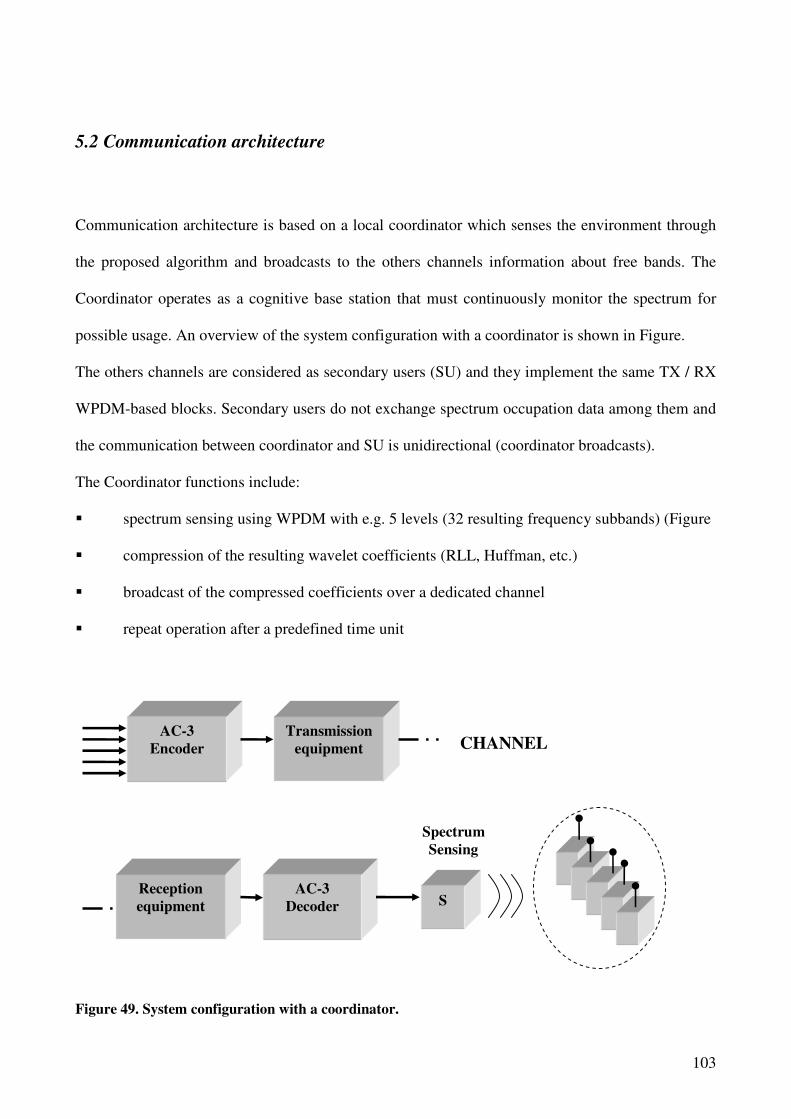
103
5.2 Communication architecture
Communication architecture is based on a local coordinator which senses the environment through
the proposed algorithm and broadcasts to the others channels information about free bands. The
Coordinator operates as a cognitive base station that must continuously monitor the spectrum for
possible usage. An overview of the system configuration with a coordinator is shown in Figure.
The others channels are considered as secondary users (SU) and they implement the same TX / RX
WPDM-based blocks. Secondary users do not exchange spectrum occupation data among them and
the communication between coordinator and SU is unidirectional (coordinator broadcasts).
The Coordinator functions include:
� spectrum sensing using WPDM with e.g. 5 levels (32 resulting frequency subbands) (Figure
� compression of the resulting wavelet coefficients (RLL, Huffman, etc.)
� broadcast of the compressed coefficients over a dedicated channel
� repeat operation after a predefined time unit
Reception
equipment
AC-3
Decoder S
AC-3
Encoder
Transmission
equipment CHANNEL
Spectrum
Sensing
Figure 49. System configuration with a coordinator.
104
Conclusions
With the demand for additional bandwidth increasing due to existing and new services, new
solutions are sought for this apparent spectrum scarcity. Although measurement studies have shown
that licensed spectrum is relatively unused across time and frequency, current government
regulatory requirements prohibit unlicensed transmissions in these bands, constraining them instead
to several heavily populated, interference-prone frequency bands. To provide the necessary
bandwidth required by current and future wireless services and applications, a new concept of
unlicensed users ”borrowing” spectrum from spectrum licensees, known as dynamic spectrum
access (DSA) is born. Simultaneously, the development of software defined radio (SDR)
technology, where the radio transceivers perform the baseband processing entirely in software,
which made them a prime candidate for DSA networks due to their ease and speed of programming
baseband operations. SDR units that can rapidly reconfigure operating parameters due to changing
requirements and conditions are known as cognitive radios (CR).
After reviewing various spectrum-sensing methods, the energy detection method was chosen to be
implemented in the design of a spectrum sensing system. Instead of using the FFT for analysing the
power content of the spectrum, we opted for an alternative method based on the wavelet
transformation and its discrete application, the Discrete Wavelet Packet Transformation (DWPT).
It is important to underline that wavelet theory is still developing. Since the use of wavelet packets
in telecommunications has been mainly studied by communications engineers, an important
potential for improvements is possible if some of the specific issues are addressed from a
mathematical point-of-view. Wavelet based communication systems have already shown a number
of advantages over conventional systems. It is expected that more is still to be pointed out as the
knowledge of this recently proposed scheme gains more interest within both the wireless
communication industry and research community.

105
Two algorithms were elaborated in this thesis: we used the wavelet packet decomposition to
efficiently estimate the spectrum and detect frequency holes through power estimation of the
subbands. The second algorithm uses histogram analysis to find non-interference zones for
secondary users transmission.
Simulation results show that the proposed algorithm can sense surrounding environment.
In chapter 4.2 a method that uses a common architecture based on WPDM for transmitting and
receiving signals was introduced. WPDM is a multiple signal transmission technique in which the
message signals are waveform coded onto wavelet packet basis functions for transmission.
Overall, the WPM schemes seem to be able to perform better than OFDM when a wavelet with
sufficiently low out-of-band energy is used. For a given wavelet, there appear to be a gain in
robustness with the increase in generating wavelet order.
In this thesis, a qualitative comparison between WPM and OFDM was presented. It was found that
WPM outperforms OFDM with respect to BER in a WLAN environment since perfect
reconstruction and orthogonality are always guaranteed. Thus, adaptive wavelet packet modulation
is a very attractive research area that will be addressed in the future.
Finally, we have presented an applicative scenario where audio information is coded by AC-3.
Therefore, we can conclude that the proposed scheme can be used as a valid cognitive system and
applied to different wireless scenarios.

106
Bibliography
REFERENCES
INTRODUCTION
[1] FCC, “Notice of Proposed Rulemaking, in the Matter of Unlicensed Operation in the TV
Broadcast Bands (ET Docket no. 04-186) and Additional Spectrum for Unlicensed Devices
below 900 MHz and in the 3 GHz Band (ET Docket no. 02-380), FCC 04-113,” May 2004.
[2] FCC, “Spectrum Policy Task Force Report (ET Docket no. 02-135),” Nov. 2002.
[3] J. Mitola and G. Q. Maguire, “Cognitive Radio: Making Software Radios More Personal,”
IEEE Pers. Commun., vol. 6, no. 4, Aug. 1999, pp. 13–18.
[4] FCC, “Notice of Proposed Rulemaking, in the Matter of Facilitating Opportunities for
Flexible, Efficient and Reliable Spectrum Use Employing Cognitive Radio Technologies
(ET Docket no. 03-108) and Authorization and Use of Software Defined Radios (ET Docket
no. 00-47), FCC 03-322,” Dec. 2003.
CAP. I
[1] D. Cabric, S. M. Mishra, and R. W. Brodersen, ``Implementation issues in spectrum sensing
for cognitive radios,'' in Proc. Asilomar Conf. on Signals, Systems, and Computers, Nov. 7-
10, 2004, vol. 1, pp. 772-776.
[2] Amit Kataria, “Cognitive Radios – Spectrum Sensing Issues”. A Thesis presented to the
Faculty of the Graduate School at the University of Missouri-Columbia, December 2007.

107
[3] N.M. Neihart, S. Roy, and D.J. Allstot, "A parallel multi-resolution sensing technique for
multiple antenna cognitive radios ", IEEE International Symposium on Circuits and
Systems, May 2007, pp. 2530-2533.
[4] Soo-Young Chang, “Analysis of Proposed Sensing Schemes: IEEE 802.22-06/0032r0”,
February 2006.
[5] Lakshmi Thanayankizil, and Aravind Kailas, “Spectrum Sensing Techniques (II): Receiver
Detection and Interference Management”, 2008.
[6] X. Liu and S. Shankar, “Sensing-based opportunistic channel access,” ACM Journal on
Mobile Networks and Applications (MONET), Vol. 11, No. 1, Feb. 2006, p. 577-591.
[7] Nabeel Ahmed, David Hadaller, and Srinivasan Keshav, “GUESS: Gossiping Updates for
Efficient Spectrum Sensing,” ACM MobiCom Workshop on Decentralized Resource
Sharing in Mobile Computing and Networking (MobiShare-06), Los Angeles, USA, Sep.
2006.
[8] Robert Brodersen, Adam Wolisz, Danijela Cabric, Shridhar Mubaraq Mishra, and Daniel
Willkomm, “CORVUS: A Cognitive Radio Approach for Usage of Virtual Unlicensed
Spectrum,” Berkeley Wireless Research Center (BWRC) White paper, 2004.
[9] Shankar, N.S. Cordeiro, C. Challapali, K. “Spectrum agile radios: utilization and
sensing architectures “, DySPAN 2005 Philips Res. USA, Briarcliff Manor, CA.
[10] S. M. Mishra, A. Sahai, and R. W. Brodersen, “Cooperative sensing among cognitive
radios,” Proc. IEEE 2006 Intl. Conf. on Communications (ICC ’06), Vol. 4, Piscataway, NJ:
IEEE Press, 2006, pp. 1658–1663.
[11] O. Simeone, J. Gambini, U. Spagnolini and Y. Bar-Ness, “Cooperation and cognitive radio,”
Proc. IEEE CogNet Workshop, 2007.
[12] G. Ghurumuruhan and Y. (G.) Li, “Cooperative spectrum sensing in cognitive radio: Part II:
multiuser networks,” accepted by IEEE Transactions on Wireless Communications, Nov.
2006.
108
[13] Ivan Cosovic, Friedrich K. Jondral, Milind M. Buddhikot, and Ryuji Kohno, “Cognitive
Radio and Dynamic Spectrum Sharing Systems”. In EURASIP Journal on Wireless
Communications and Networking, 2008.
[14] N. Sai Shankar, C. Cordeiro and K. Challapali, ``Spectrum agile radios: utilization and
sensing architectures,'' Proc. DySPAN'05, Baltimore, USA, Nov. 8-11, 2005, pp. 160-169.
CAP. II
[1] D. Čabrić, R. Brodersen, “Physical Layer Design Issues Unique to Cognitive Radio
Systems”. 16th IEEE International Symposium on Personal Indoor and Mobile Radio
Communications, (PIMRC 2005), September 11-14, 2005.
[2] R. Rajbanshi, Q. Chen, A. M. Wyglinski, J.B. Evans and G. J. Minden. “Comparative Study
of Frequency Agile Data Transmission Schemes for Cognitive Radio Transceivers”. In
ACM International Conference Proceeding Series; Vol. 222, Proceedings of the first
international workshop on Technology and policy for accessing spectrum Boston, 2006.
[3] Sorour Falahati, Arne Svensson “Adaptive Modulation Systems for Predicted Wireless
Channels,” From IEEE Transactions on Communications, Vol. 52, No. 2, Feb. 2004.
[4] B. Wild and K. Ramchandran, “Detecting primary receivers for cognitive radio
applications”. In Proc. 1st IEEE Symp. New Frontiers in Dynamic Spectrum Access
Networks (DySPAN’05), Baltimore, USA, Nov. 8–11, 2005, pp. 124–130.
[5] K. Hamdi, W. Zhang, and K. B. Letaief, “Power Control in Cognitive Radio Systems Based
on Spectrum Sensing Side Information”. In: IEEE International Conference 24-28 June
2007, pp. 5161 – 5165.
[6] S. Kim, H. Jeon, H. Lee, and J. S. Ma, "Robust Transmission Power and Position Estimation
in Cognitive Radio," International Conference on Information Networking (ICOIN'07),
2007.

109
[7] D. Cabric; M.S.W. Chen; D.A. Sobel; Jing Yang; R.W. Brodersen, “Future wireless
systems: UWB, 60GHz, and cognitive radios," In: Custom Integrated Circuits Conference,
2005. Proceedings of the IEEE 2005, 21-21 Sept. 2005, pp. 793-796.
[8] P.S. Hall, P. Gardner, J. Kelly, E. Ebrahimi, M.R. Hamid, and F. Ghanem “Antenna
Challenges in Cognitive Radio”. In: Proc. ISAP 08, Taiwan, Oct. 2008.
[9] Di Taranto, R. Nishimori, K. Popovski, P. Yomo, Takatori, Y. Prasad, R. Kubota “Simple
Antenna Pattern Switching and Interference-Induced Multi-Hop Transmissions for
Cognitive Radio Networks“, DySPAN 2007, 2nd IEEE International Symposium on New
Frontiers in Dynamic Spectrum Access Networks. 17- 20 April 2007, pp 543 – 546.
[10] K. Takeuchi, T. Fukuhara, S. Nomura, S. Yamamoto, “Cognitive Radio Using Multi-
transmission Links - a Novel Approach Effective in Metropolitan Areas”. In: Cognitive
Radio Oriented Wireless Networks and Communications, 2007. CrownCom 2007. , 1-3
Aug. 2007, pp. 291-297.
[11] B. Ackland, D. Raychaudhuri, M. Bushnell, C. Rose, I. Seskar, T. Sizer, D. Samardzija, J.
Pastalan, A. Siegel, J. Laskar, S. Pinel and K. Lim, “High Performance Cognitive Radio
Platform with Integrated Physical and Network Layer Capabilities”, Interim Technical
Report for the NeTS-ProWiN Project, Rutgers University, July 2005.
CAP. III
[1] J.N. Bradley and C.M. Brislawn. The wavelet/scalar quantization compression standard for
digital fingerprint images. IEEE Circuits and Systems, 3:208–208, May 1994.
[2] C.M. Chang and T.S. Liu. Application of discrete wavelet transform to repetitive control.
Proceedings of the ACC, pages 4560–4565, May 2002.
[3] P.F. Craigmile and D.B. Percival. Wavelet-based trend detection and estimation. Technical
report, University of Washington, Seattle, December 2000.

110
[4] P. Cruz, A. Mendes, and F.D. Magalh aes. Using wavelets for solving PDEs: and adaptive
collocation method. Chemical Engineering Science, 56:3305–3309, 2001.
[5] I. Daubechies. Ten Lectures on Wavelets. Society for Industrial and Applied Mathematics,
1992. ISBN 0-89871-274-2.
[6] L. Daudet, P. Guileemain, R. Kronland-Martinet, and B. Torr´esani. Low bit-rate audio
coding with hybrid representations, pages 1–4, January 2000.
[7] B. de Kraker. A numerical-experimental approach in structural dynamics. Technical report,
Eindhoven University of Technology, Department of Mechanical Engineering, 2000.
[8] D.L. Donoho and I.M. Johnstone. Threshold selection for wavelet shrinkage of noisy data.
IEEE, pages 24a–25a, 1994.
[9] H. Du and S.S. Nair. Identification of friction at low velocities using wavelet basis function
network. Proceedings of the American Control Conference, pages 1918–1922, June 1998.
[10] R.M.L. Ellenbroek. Time-frequency adaptive iterative learning control. Master thesis,
Eindhoven University of Technology, February 2003.
[11] R.F. Favero. Compound wavelets: wavelets for speech recognition. IEEE, pages 600–603,
1994.
[12] S. Grgic, M. Grgic, and B. Zovko-Cihlar. Performance analysis of image compression using
wavelets. IEEE Transactions on Industrial Electronics, 48(3):682–695, June 2001.
[13] D. Huang and Y. Jin. The application of wavelet neural networks to nonlinear predictive
control. IEEE, pages 724–727, 1997.
[14] J.F. James. A student’s guide to Fourier transforms. Cambridge University Press, first
edition, 1995. ISBN 0-521-46829-9.
[15] J.J. Kok and M.J.G. van de Molengraft. Signal analysis. Technical report, Eindhoven
University of Technology, Department of Mechanical Engineering, 2002.
[16] M. Misiti, Y. Misiti, G. Oppenheim, and J-M Poggi. Wavelets Toolbox Users Guide. The
MathWorks, 2000. Wavelet Toolbox, for use with MATLAB.

111
[17] L. Pasti, B. Walczak, D.L. Massart, and P. Reschiglian. Optimization of signal denoising in
discrete wavelet transform. Chemometrics and intelligent laboratory systems, 48:21–34,
1999.
[18] T.A. Ridsdill-Smith. Wavelet design of time-varying filters. February 2002.
[19] P. Rieder and J.A. Nossek. Implementation of orthogonal wavelet transforms and their
applications. IEEE, pages 489–498, 1997.
[20] O. Rioul and M. Vetterli. Wavelets and signal processing. IEEE SP Magazine, pages 14–38,
October 1991.
[21] M.G.E. Schneiders. Wavelets in control engineering. Master’s thesis, Eindhoven University
of Technology, August 2001. DCT nr. 2001.38.
[22] C. Schremmer, T. Haenselmann, and F. B¨omers. A wavelet based audio denoiser. January
2001.
[23] A. Skodras, C. Christopoulos, and T. Ebrahimi. The JPEG 2000 still image compression
standard. IEEE Signal Processing Magazine, pages 36–58, September 2001.
[24] G. Strang and T. Nguyen. Wavelets and Filter Banks. Wellesley-Cambridge Press, second
edition, 1997. ISBN 0-9614088-7-1.
[25] K. Subramaniam, S.S. Dlay, and F.C. Rind. Wavelet transforms for use in motion detection
and tracking application. IEEE Image processing and its Applications, pages 711–715, 1999.
[26] N. Sureshbabu and J.A. Farrell. Wavelet-based system identification for nonlinear control
IEEE Transactions on Automatic Control, 44(2):412–417, February 1999.
[27] W. Sweldens. Construction and Applications of Wavelets in Numerical Analysis. Phd thesis,
Department of Computer Science, Catholic University of Leuven, Belgium, May 1995.
[28] M. Tico, P. Kuosmanen, and J. Saarinen. Wavelet domain features for fingerprint
recognition IEEE Electronic Letters, 37(1):21–22, January 2001.
[29] B.E. Usevitch. A tutorial on modern lossy wavelet image compression: Foundations of
JPEG 2000. IEEE Signal Processing Magazine, pages 22–35, September 2001.
112
[30] A. van Nevel. Texture classification using wavelet frame decomposition. IEEE Signals,
Systems and Computers, 1997.
[31] E. Visser, T. Lee, and M. Otsuka. Speech enhancement in a noisy car environment. pages
272–276, December 2001.
[32] J. Walter, B. Arnrich, and C. Scheering. Learning fine positioning of a robot manipulator
based on Gabor wavelets. IEEE, pages 137–142, 2000.
[33] Y. Wang, S. Kwon, A. Rgan, and T. Rohlev. System identification of the linac RF system
using a wavelet method and its applications in the SNS LLRF control system. Proceedings
of the Particle Accelerator Conference, Chicago, pages 1613–1615, 2001.
[34] J. Xu and Y. Tan. Nonlinear adaptive wavelet control using constructive wavelet networks.
ACC, pages 624–629, 2001.
[35] B. Zhang, D. Wang, and Y. Ye. Wavelet transform-based frequency tuning ILC. IEEE
Transactions on systems, man and Cybernetics - Part B, 35(1), 2005.
CAP. IV
[1] I. Daubechies, Ten Lectures on Wavelets. Philadelphia, PA: SIAM,1992.
[2] G. Strang and T. Nguyen, Wavelet and Filter Banks. Wellesley, MA: Wellesley-Cambridge
Univ. Press, 1996.
[3] G. Strang, “Wavelets and dilation equations: A brief introduction,” SIAM Rev., vol. 31, pp.
614–627, Dec. 1989.
[4] D. Čabrić, R. Brodersen, “Physical Layer Design Issues Unique to Cognitive Radio
Systems”. 16th IEEE International Symposium on Personal Indoor and Mobile Radio
Communications, (PIMRC 2005), September 11-14, 2005.
[5] R. Rajbanshi, Q. Chen, A. M. Wyglinski, J.B. Evans and G. J. Minden. “Comparative Study
of Frequency Agile Data Transmission Schemes for Cognitive RadioTransceivers”. In ACM
113
International Conference Proceeding Series; Vol. 222, Proceedings of the first international
workshop on Technology and policy for accessing spectrum Boston, 2006.
[6] Sorour Falahati, Arne Svensson “Adaptive Modulation Systems for Predicted Wireless
Channels,” From IEEE Transactions on Communications, Vol. 52, No. 2, Feb. 2004.
[7] B. Wild and K. Ramchandran, “Detecting primary receivers for cognitive radio
applications”. In Proc. 1st IEEE Symp. New Frontiers in Dynamic Spectrum Access
Networks (DySPAN’05), Baltimore, USA, Nov. 8–11, 2005, pp. 124–130.
[8] K. Hamdi, W. Zhang, and K. B. Letaief, “Power Control in Cognitive Radio Systems Based
on Spectrum Sensing Side Information”. In: IEEE International Conference 24-28 June
2007, pp. 5161 – 5165.
[9] A. Jamin, P. Mähönen, “Wavelet Packet Modulation for Wireless Communications”. In:
Wireless Communications & Mobile Computing Journal, March 2005, Vol. 5, Issue 2.
[10] P. Siohan, C. Siclet, and N. Lacaille, “Analysis and design of ofdm/oqam systems based on
filterbank theory,” IEEE Trans. Signal Processing, vol. 50, no. 5, May 2002.
[11] I. Daubechies, “Orthonormal bases of compactly supported wavelets,” Commun. Pure
Applied Math., vol. XLI, no. 7, pp. 909–996, Oct. 1988.
CAP. V
[1] Digital Audio Compression Standard (AC-3, E-AC-3) Revision B, 14 June 2005.
[2] G. Davidson, L. Fielder, and M. Antill, "Low-Complexity Transform Coder for Satellite
Link Applications," AES 89th Convention, Los Angeles, Sept. 1990, Preprint 2966.
[3] Advanced Television System Committee, Digital Audio Compression Standard (AC-3), 20
Dec. 95.
[4] L. Fielder and G. Davidson, "AC-2: A Family of Low-Complexity Transform-Based Music
Coders," 1991 AES Workshop on Digital Audio, London, Oct. 1991.

114
[5] ATSC N52, “Digital Audio Compression (AC-3) Standard” United States Advanced
Television Systems Committee.


![Compendium [G.marciani] - Telecomunicazioni](https://img.pdfslide.net/doc/110x75/55cf860f550346484b93db4a/compendium-gmarciani-telecomunicazioni.jpg)