Aerodynamic and heat transfer studies in a combustor-fired

Louisiana State UniversityLSU Digital Commons

LSU Master's Theses Graduate School

2009

Aerodynamic and heat transfer studies in acombustor-fired, fixed-vane cascade with filmcoolingJames William PostLouisiana State University and Agricultural and Mechanical College, [email protected]

Follow this and additional works at: https://digitalcommons.lsu.edu/gradschool_theses

Part of the Mechanical Engineering Commons

This Thesis is brought to you for free and open access by the Graduate School at LSU Digital Commons. It has been accepted for inclusion in LSUMaster's Theses by an authorized graduate school editor of LSU Digital Commons. For more information, please contact [email protected].

Recommended CitationPost, James William, "Aerodynamic and heat transfer studies in a combustor-fired, fixed-vane cascade with film cooling" (2009). LSUMaster's Theses. 2497.https://digitalcommons.lsu.edu/gradschool_theses/2497

https://digitalcommons.lsu.edu?utm_source=digitalcommons.lsu.edu%2Fgradschool_theses%2F2497&utm_medium=PDF&utm_campaign=PDFCoverPages

https://digitalcommons.lsu.edu/gradschool_theses?utm_source=digitalcommons.lsu.edu%2Fgradschool_theses%2F2497&utm_medium=PDF&utm_campaign=PDFCoverPages

https://digitalcommons.lsu.edu/gradschool?utm_source=digitalcommons.lsu.edu%2Fgradschool_theses%2F2497&utm_medium=PDF&utm_campaign=PDFCoverPages

https://digitalcommons.lsu.edu/gradschool_theses?utm_source=digitalcommons.lsu.edu%2Fgradschool_theses%2F2497&utm_medium=PDF&utm_campaign=PDFCoverPages

http://network.bepress.com/hgg/discipline/293?utm_source=digitalcommons.lsu.edu%2Fgradschool_theses%2F2497&utm_medium=PDF&utm_campaign=PDFCoverPages

https://digitalcommons.lsu.edu/gradschool_theses/2497?utm_source=digitalcommons.lsu.edu%2Fgradschool_theses%2F2497&utm_medium=PDF&utm_campaign=PDFCoverPages

mailto:[email protected]

AERODYNAMIC AND HEAT TRANSFER STUDIES IN A COMBUSTOR-FIRED, FIXED-VANE CASCADE WITH FILM

COOLING

A Thesis

Submitted to the Graduate Faculty of the Louisiana State University and

Agricultural and Mechanical College in partial fulfillment of the

requirements for the degree of Master of Science in Mechanical Engineering

in

The Department of Mechanical Engineering

By James William Post

B.S.M.E., Louisiana State University, 2006 May 2009

ii

ACKNOWLEDGEMENTS

First and foremost, I would like to thank my parents, Jim and Amelie Post. Without their

support and guidance, I could have never gotten this far in my education. Secondly, I would like

to thank my major professor, Dr. Sumanta Acharya. Had he not offered me a student worker

position back in 2004, I might not have chosen this path. Deepest thanks go to Dr. Janice C.

Crosby, who has motivated me to do better and to try harder in all aspects of life. Her affection

and moral support have helped me realize some of my true potential. I thank Nathan Branch and

Jeff Wilbanks, all my engineering friends, and any friends I have met through playing music.

I would also like to acknowledge all my fellow graduate students who have had some

impact on my journey. Tony Giglio, Curtis Hebert, Pritish Parida, Ben Rawls, and Del Segura

have all helped me through small stumbling points in some way. Many thanks go to Mr. Jim

Layton, Mr. Ed Martin, Mr. Barry Savoy, Mr. Paul Rodriguez, and Mr. Don Colvin for assisting

me with everything I have fabricated in the ME and ChemE shops. Thanks also go to Mr.

Charles Smith for always allowing me use of his forklift. Mr. Tony Lombardo and Mr. Jim

Mayne have both been key to the safe construction and operation of the high-pressure N.G. line.

I am grateful for the efforts of many parties outside of the university. Mr. Tommy

Blanchard of Trade Construction Co. selflessly worked with me when the time came to fabricate

pipelines. He also provided insights and guidance at crucial junctures in this lab’s design. Mr.

Bob Graybill of Stahl Inc., Mr. Scott Ralston of ATK, Dr. Rudy Martinez of Farmer’s Marine

Copperworks, and, finally, Dr. Ronald S. Bunker of GE Energy have all contributed considerable

time and effort in this facility’s evolution. The US Department of Energy (DOE) through the

University Turbine Systems Research (USTR) Program has provided additional funding for this

project. I would finally like to acknowledge the Louisiana Board of Regents (BoR) and the Clean

Power and Energy Research Consortium (CPERC) for their local monetary support.

iii

TABLE OF CONTENTS

ACKNOWLEDGEMENTS ii

LIST OF TABLES v

LIST OF FIGURES vi

ABSTRACT xiii

CHAPTER 1: INTRODUCTION 1

CHAPTER 2: LITERATURE REVIEW 5 2.1: Endwall Contouring 5 2.2: Endwall Contouring with Computational Aids 12

CHAPTER 3: FACILITY DESIGN AND SETUP 20 3.1: Main Equipment 20 3.1.1 Test Sections 20 3.1.2 Pressure Vessel 24 3.1.3 Combustor and Fuel Control System 31 3.2: Facility Design and Layout 37 3.2.1 Inlet Air 38 3.2.2 Natural Gas 49 3.2.3 Exhaust 51 3.3: Film Cooling Line Design 58 3.4: Current Facility Layout and Operation 67 3.5: Instrumentation and Experimental Uncertainty 76

CHAPTER 4: EXPERIMENTAL RESULTS 92 4.1: Pressure Data 92 4.2: Normalized Metal Temperature (NMT) Data 95 4.3: Heat Transfer Coefficient (HTC) Data 110

CHAPTER 5: CONCLUSIONS AND RECOMMENDATIONS 127

REFERENCES 131

APPENDIX A: CONAX SEALING GLAND INFORMATION 133

APPENDIX B: STAHL COMBUSTOR DRAWINGS 134

APPENDIX C: LABVIEW PROGAMS 137

iv

APPENDIX D: HF GAGE CALIBRATION CURVE 140

APPENDIX E: MATLAB PROGRAMS 141

APPENDIX F: AUXILIARY NMT DATA 142

VITA 155

v

LIST OF TABLES

Table 3.1: Total Errors for DSA 3217 and cFP Modules 81

Table 3.2: Total Error for Film Cooling Air Flow Instrumentation 87

Table 3.3: Theoretical Blowing Ratio Uncertainty Summary 90

Table 4.1: Interrelationship of TR, M, and DR 109

vi

LIST OF FIGURES

Figure 3.1.1: Test Section Solid Model 21

Figure 3.1.2: Picture of Test Section after Running Heated Flow Tests 22

Figure 3.1.3: Test Section Top View with Sapphire Windows 23

Figure 3.1.4: Pressure Vessel Inlet Transition Piece 24

Figure 3.1.5: Schematic of Pressure Vessel Internals 25

Figure 3.1.6: Large Sapphire Window Assembly 26

Figure 3.1.7: Cover Plate, Supply Box, and Conax Glands 27

Figure 3.1.8: Improved Bellows Assembly Parts 28

Figure 3.1.9: Installed Bellows Assemblies before Retrofit 28

Figure 3.1.10: New Bellows Assemblies 29

Figure 3.1.11: Adapter Piece Close-up 29

Figure 3.1.12: Third Section of the Pressure Vessel with Fike Burst Disk Assembly 30

Figure 3.1.13: Installed Burst Disk Assembly 30

Figure 3.1.14: Real Life Combustor Fabricated by Stahl Inc. 31

Figure 3.1.15: Combustor Inlet Shell (view from above) 33

Figure 3.1.16: Bottom Section of Fuel Control System 34

Figure 3.1.17: Upper Section of Fuel Control System 35

Figure 3.1.18: NEMA-4x Rated Combustor Control Box and Controls 36

Figure 3.2.1: Compressors, Dryers, and Tank Behind the Lab 38

Figure 3.2.2: Atlas CopCo Model GA-315 Internals 39

Figure 3.2.3: Zander Model KN-32 Air Dryers and Their Control Panels 40

Figure 3.2.4: Inlet Fisher Globe Valve with Diaphragm Actuator and Valve Controller 41

Figure 3.2.5: Flowmetrics Model FM-64F1T1ALDT Flow Meter 42

vii

Figure 3.2.6: Early Floor Plan Schematic 43

Figure 3.2.7: Another Schematic of an Early Floor Plan 44

Figure 3.2.8: Schematic of Third Floor Plan 44

Figure 3.2.9: Final Inlet Air Line Design Schematic 45

Figure 3.2.10: Inlet Air Pipeline 46

Figure 3.2.11: Stainless Steel Tube Window Cooling Assembly inside Pressure Vessel 47

Figure 3.2.12: Outside Sapphire Window Cooling Air Supply Pipelines 48

Figure 3.2.13: Natural Gas Pipeline outside the Lab 49

Figure 3.2.14: Fuel Control System Standing beside Combustor 50

Figure 3.2.15: Natural Gas Pipeline inside Lab and Connected to Fuel Control System 51

Figure 3.2.16: Fisher Exhaust Control Valve 52

Figure 3.2.17: Schematic of Main Exhaust Line with Valve 53

Figure 3.2.18: A Fike Burst Disk 54

Figure 3.2.19: Early Floor Plan Schematic with Short Emergency Line 55

Figure 3.2.20: Schematic of Fabricated Exhaust Lines 56

Figure 3.2.21: Exhaust Pipelines Installed in the Lab 57

Figure 3.3.1: Schematic of Film Cooling Line Design 58

Figure 3.3.2: Actual Film Cooling Line with Fisher Globe Valve 59

Figure 3.3.3: Estimated Film Cooling Requirements for Endwall and Vane 62

Figure 3.3.4: Estimated Film Cooling Requirements for the Upstream Contour Section 62

Figure 3.3.5: Upstream Contour Supply Line inside Pressure Vessel 63

Figure 3.3.6: Upstream Contour Needle Valve 64

Figure 3.3.7: Power Estimates for Film Cooling Air Heater 66

Figure 3.4.1: Schematic of Current Lab Layout 67

viii

Figure 3.4.2: Fisher DPR950 Controllers and Flowmetrics 924-ST2 Flow Computer 68

Figure 3.4.3: Actual Lab Picture Taken from Control Room 69

Figure 3.4.4: Close-up View of Endwall and Vane Supply Lines 71

Figure 3.4.5: Transition Piece Utilized for Collecting Upstream Data 72

Figure 3.4.6: Scanivalve Model 3217 DSA and NI cFP System 74

Figure 3.5.1: A Medtherm Model 4H-50-36-36-20753 Heat Flux Gage 77

Figure 3.5.2: Heat Transfer Endwall Inner Plenum with Thermal Sealant 78

Figure 3.5.3: Absolute Accuracy Chart for the cFP-TC-120 Input Module [14] 80

Figure 4.1.1: Endwall CF PR Contour Plot 92

Figure 4.1.2: Endwall HF PR Contour Plot 92

Figure 4.1.3: Vane Midspan Pressure Ratio Data 94

Figure 4.2.1: EW NMT: M = 0.5, TR = 1.6 96

Figure 4.2.2: EW NMT: M = 1.0, TR = 1.6 96

Figure 4.2.3: EW NMT: M = 1.5, TR = 1.6 96

Figure 4.2.4: EW NMT: M = 2.0, TR = 1.6 96

Figure 4.2.5: EW NMT: M = 2.75, TR = 1.6 97

Figure 4.2.6: EW NMT: M = 3.0, TR = 1.6 97

Figure 4.2.7: Vane NMT Line Plots for Nominal TR of 1.55 98

Figure 4.2.8: EW NMT: M = 0.75, TR = 1.9 99

Figure 4.2.9: EW NMT: M = 1.0, TR = 1.9 99

Figure 4.2.10: EW NMT: M = 1.5, TR = 1.9 100

Figure 4.2.11: EW NMT: M = 2.0, TR = 1.9 100

Figure 4.2.12: EW NMT: M = 2.2, TR = 1.9 101

Figure 4.2.13: EW NMT: M = 2.4, TR = 1.9 101

ix

Figure 4.2.14: EW NMT: M = 2.7, TR = 1.9 101

Figure 4.2.15: EW NMT: M = 2.9, TR = 1.9 101


Figure 4.2.17: EW NMT: M = 0.25, TR = 1.1 104

Figure 4.2.18: EW NMT: M = 0.5, TR = 1.1 104

Figure 4.2.19: EW NMT: M = 1.0, TR = 1.1 104

Figure 4.2.20: EW NMT: M = 1.5, TR = 1.1 104

Figure 4.2.21: EW NMT: M = 2.0, TR = 1.1 105

Figure 4.2.22: EW NMT: M = 2.5, TR = 1.1 105

Figure 4.2.23: EW NMT: M = 2.75, TR = 1.1 106

Figure 4.2.24: EW NMT: M = 3.0, TR = 1.1 106


Figure 4.2.26: EW Overall NMT for Different M at Nominal TR of 1.1, 1.6, and 1.9 108

Figure 4.2.27: Vane Overall NMT for Different M at Nominal TR of 1.1, 1.5, and 1.8 109

Figure 4.3.1: EW HTC: M = 0.5, TR = 1.55 111

Figure 4.3.2: EW HTC: M = 1.0, TR = 1.55 111

Figure 4.3.3: EW HTC: M = 1.5, TR = 1.55 112

Figure 4.3.4: EW HTC: M = 2.0, TR = 1.55 112

Figure 4.3.5: EW HTC: M = 2.7, TR = 1.55 113

Figure 4.3.6: EW HTC: M at 3.0, TR = 1.55 113

Figure 4.3.7: Vane HTC Line Plots for Nominal TR of 1.5 114

Figure 4.3.8: Expanded Vane HTC Line Plots for Nominal TR of 1.5 114

Figure 4.3.9: EW HTC: M = 0.75, TR = 1.9 116

Figure 4.3.10: EW HTC: M = 1.0, TR = 1.9 116

x

Figure 4.3.11: EW HTC: M = 1.5, TR = 1.9 116

Figure 4.3.12: EW HTC: M = 2.0, TR = 1.9 116

Figure 4.3.13: EW HTC: M = 2.2, TR = 1.9 117

Figure 4.3.14: EW HTC: M = 2.4, TR = 1.9 117

Figure 4.3.15: EW HTC: M = 2.7, TR = 1.9 118

Figure 4.3.16: EW HTC: M = 2.9, TR = 1.9 118



Figure 4.3.19: EW HTC: M = 0.25, TR = 1.1 120

Figure 4.3.20: EW HTC: M = 0.5, TR = 1.1 120

Figure 4.3.21: EW HTC: M = 1.0, TR = 1.1 121

Figure 4.3.22: EW HTC: M = 1.5, TR = 1.1 121

Figure 4.3.23: EW HTC: M = 2.0, TR = 1.1 121

Figure 4.3.24: EW HTC: M = 2.5, TR = 1.1 121

Figure 4.3.25: EW HTC: M = 2.7, TR = 1.1 122

Figure 4.3.26: EW HTC: M = 3.0, TR = 1.1 122



Figure 4.3.29: EW Overall HTC for Different M at Nominal TR of 1.1, 1.6, and 1.9 125

Figure 4.3.30: Vane Overall HTC for Different M at Nominal TR of 1.1, 1.5, and 1.8 126

Figure A.1: Conax PGS, SPG, and DSPG Sealing Gland Information 133

Figure B.1: Stahl Combustor Drawing 33763 134



xi

Figure C.1: LabVIEW Program Front Panel Controlling Scanivalve and cFP Systems 137

Figure C.2: State Machine Structure of LabVIEW Program with Main States Shown 138

Figure C.3: LabVIEW Program "Initialize" State 139

Figure C.4: LabVIEW Program "Close Connections" State 139

Figure D.1: Typical Medtherm HF Gage Responsivity Curve 140

Figure F.1: EW NMT: M at 0.75, TR of 1.3 142








Figure F.9: EW NMT: M at 2.0,TR of 1.35 145








Figure F.17: EW Overall NMT for Different M at Nominal TR of 1.3, 1.5, and 1.8 148

Figure F.18: Vane NMT Line Plots for Nominal TR of 1.3 149

Figure F.19: Expanded Vane NMT Line Plots for Nominal TR of 1.3 150

xii

Figure F.20: Vane NMT Line Plots for Nominal TR of 1.4 151

Figure F.21: Expanded Vane NMT Line Plots for Nominal TR of 1.4 152

Figure F.22: Vane Line Plots for Nominal TR of 1.6 153

Figure F.23: Vane Overall NMT for Different M at Nominal TR of 1.3, 1.4, and 1.6 154

xiii

ABSTRACT

Pressure and heat transfer data has been generated in a high-pressure, high-temperature

vane cascade. This cascade differs from many others seen in typical low-pressure facilities using

room temperature air. Primarily, a natural gas-fired combustor generates realistic turbulence

profiles in the high-temperature exhaust gases that pass through the vane cascade. The fixed-

vane cascade test sections have film cooling holes machined into the surfaces in arrangements

that closely model configurations seen in real-life first-row nozzle guide vanes (NGV).

Theoretical coolant jet-to-crossflow blowing ratios (M) range from 0.5 to 3.0. Coolant jet-to-

crossflow theoretical density ratios (DR) used for typical tests vary between 1.0 and 2.5. A

strong relationship has been observed between blowing ratio and density ratio. Mostly due to

increased mass associated with the addition of combustion gases, pressure data for heated

crossflows shows slight decreases in crossflow-to-surface pressure ratios (PR) when compared to

non-heated data. Heat transfer data consists of normalized metal temperatures (NMT) and heat

transfer coefficients (HTC). All sets of NMT and HTC data at different crossflow-to-coolant

temperature ratios (TR) show general increases with rising blowing ratio. Temperature ratios can

be altered with the combustor’s integrated fuel control system. NMT data typically indicates

better coolant performance for lower temperature ratios. Averaged overall endwall NMT values

go through regions dependent on blowing ratio where varying the temperature ratio gives best

performance. Higher blowing ratios cause lower NMT generally due to reduced coolant coverage

along the vane suction surface (SS). HTC data reflects similar trends as the NMT data. At low

blowing ratios, high HTC values near the passage throat on the endwall signify defined flow

acceleration toward the throat. Higher HTCs evolve on the endwall in the region upstream of the

throat with increases in coolant associated with higher blowing ratios. Vane HTC data shows

xiv

best performance near the leading edge of the midspan plane where many film cooling holes

have been located.

1

CHAPTER 1: INTRODUCTION

Ever since the days of Archimedes and Hero of Alexandria, great philosophers and

scientists have laboriously searched for ways to convert naturally occurring fluid energy into

usable forms. From the sails of seafaring vessels of early civilizations to the modern supersonic

jets, methods for extracting fluid power constantly evolve as growing insights into the visible

and invisible world breed newer technologies. A certain class of machines commonly called

turbomachinery demonstrates a very intuitive process for the conversion of fluid energy.

Compressors, turbines, and other turbomachines all rely on some mode of exchange between

fluid energy and rotational energy. Typically, interactions between the fluid and shaft-mounted

objects, known as blades or vanes, require some form of rotation about the shaft axis.

Compressors and pumps impart energy to the fluid by raising pressure through velocity changes

governed by Bernoulli’s principle. Turbines extract rotational energy from fluid expansion.

For many centuries, complete steam engines usually consisting of pumps and turbines

have had wide application since water acts as the working fluid. In the late eighteenth century,

Englishman John Barber took out the first patent for a concept later to become the gas-based

turbine engine. A few decades later, American George Brayton developed the ideas of Barber to

create a continuous combustion engine that operated on the now famous Brayton cycle. Serving

as the foundation for modern gas turbines, this air-based thermodynamic cycle consists of an

adiabatic compression, an isochoric heat addition process, an adiabatic expansion through a

turbine, and an isochoric heat rejection process that completes the cycle. Heat addition usually

comes from the combustion of a fuel added to the compressed air while heat rejection can take

many forms such as exhausting the expanded gases to the atmosphere.

In the early twentieth century, further development allowed Norwegian Ægidius Elling to

construct the first modern gas turbine engine that produced more power than its components

2

required. This technological milestone resulted in an explosion of research resulting in General

Electric’s formation of a gas turbine division. Even famed Serbian engineer Nikola Tesla

developed a blade-less gas turbine operating on boundary layer drag. Still the most important

contribution came in the 1930’s from Englishman Sir Frank Whittle who explored the

application of gas turbines to enable jet propulsion. Whittle’s engine had its first successful use

in 1937.

Ever since these inventors revolutionized power generation, electricity plants, aircraft,

and any other machines that require high output power devices often meet their needs through

use of a gas turbine engine. Even though the hot gas expansion concept seems rather

straightforward in nature, such a simple idea does not nearly completely describe the intricate

fluid flow problems associated with the gas expansion. Fluid energy imperfectly creates

rotational torque via the lift force on the turbine blades. Some of this energy becomes lost when

it dissipates through non-axial circulation within passages between blades. Driven by adverse

blade passage pressure gradients, so-called secondary flows contribute very little to the primary

bulk motion through the passage or channel. These structures create unrecoverable aerodynamic

losses that considerably reduce turbine efficiency. Furthermore, the turbine can extract increased

amounts of work if the gas enters at a higher temperature. As experienced by Elling and Whittle,

materials able to withstand higher operating temperatures would allow hotter fluids to expand

through the turbine and thereby raise efficiency.

In an age of exponentially rising fuel costs and experimental fuel sources, inefficient

turbine designs can increase fuel consumption and overall cost of operation. With this in mind, a

few generations of researchers have tirelessly searched for ways to improve design efficiency

through studying methods that have the potential to reduce secondary circulations and to raise

inlet temperatures. To date, the most promising schemes appear to be contouring endwalls,

3

which join the cascaded blades to the rotating shaft, and film cooling by the injection of air jets

through holes machined on the endwall and blade surfaces. Inlet blade passage boundary layers

increase freestream turbulence and favor secondary circulation as these layers grow. Secondary

flows appear mostly driven by the radial pressure gradient inherent in a turbine design consisting

of angularly cascaded blades. Higher pressure acting on a blade’s pressure surface (PS) creates

lift by desiring to meet the lower pressure on the blade’s suction surface (SS). A cascaded

configuration positions a pressure surface across the passage from a suction surface resulting in

some flow migration occurring in the radial direction. Endwall shaping/contouring regimes

become most effective when this pressure gradient can be reduced. Attempts to raise inlet

temperatures have resulted in many a turbine failure. The most catastrophic of these occur when

blades melt away from the endwalls. Small secondary flows at the blade-endwall interface bring

higher temperature mainstream fluid to this area. Increased heat transfer shortens the lifespan of

the blades. External surface film cooling has been developed as a means for reducing

temperatures near the blade-endwall interface. This method coats the blade and endwall surfaces

with thin “films” of cooler air, which not only reduces surface temperatures but also disrupts

secondary flow structures bringing hotter fluid to these surfaces. Endwall contouring and film

cooling form the basis for the research presented in this thesis.

In chapter two, a literature review describes the early investigations into endwall

contouring from simple inlet-to-exit area reduction to complex modern profiles obtained through

extensive computer modeling. The third chapter formally introduces the major parts of a facility

used to conduct the above-mentioned research. This chapter’s second section holds extensive

details of this facility’s design and assembly. All pertinent information on the film cooling air

supply system has been thoroughly discussed in the third section of the third chapter. After that,

another section describes this facility’s current setup as well as how one can operate it. This

4

chapter concludes with a section presenting the key instrumentation and a detailed uncertainty

analysis of all applicable parameters such as pressure ratio (PR) and blowing ratio (M). Pressure

and heat transfer data can be found in the fourth chapter. Contour plots show endwall

distributions of pressure ratios (PR), normalized metal temperatures (NMT), and heat transfer

coefficients (HTC). Line plots have been chosen to represent distributions of those parameters

along the vane surfaces. Separate plots of spatially averaged overall quantities summarize

normalized metal temperature (NMT) and heat transfer coefficient (HTC) data for the endwall

and vane surfaces. Commentary on these data sets indicates the author’s interpretation of these

results and speculations about their meaning. A summary of key findings and recommendations

for future study comprise the last chapter. References and appendices follow, and a vita

presented on the author concludes this thesis.

5

CHAPTER 2: LITERATURE REVIEW

2.1: Endwall Contouring

An experiment by Sieverding, Van Hove, and Boletis (1984) investigated the flow field

in a low-speed, low aspect ratio turbine nozzle by collecting pressure data using a four-hole

pressure probe. [1] Much study at the time of the paper’s publication involved validation of

boundary layer theories that attempted to predict the flow field through the vane cascade.

Sieverding, et al. even admit that the age of solving equations using elegant mathematics has met

its decline through raw data collection that can be used to fit an applicable correlation.

The experimental apparatus consisted of a blade cascade with guidevanes and a collateral

inlet endwall. An untwisted profile from tip to endwall was chosen for the 21 blades. The

measurement probe took data in 12 x/Cax (pitch/axial chord) planes along three stream profiles at

varying heights (y/H’s). Smoke visualization through a laser light sheet technique displayed

passage side and suction side legs of “horseshoe”-shaped vortex structures in the pitchwise

direction. [1] Most curiously, the passage vortex and pressure side leg of the horseshoe vortex

rotated in the same direction, which made the two indiscernible to the experimenters.

Sieverding, et al. presented further data that documented boundary layer “evolution”

along the three stream profiles (positioned at ~ ¼, ½, and ¾ the distance of the channel from the

pressure surface). The flow angles (’s), which give direction to the stream, were calculated

using a two-dimensional singularity method found in publications from Martensen. Radial

pressure gradients expectedly affected boundary layer structures. Inherent to a vane/blade

cascade’s design, these radial pressure gradients cause the velocity gradient needed for the

vane’s lift function. As observed, radial pressure gradients increase from pressure side to suction

side. Both the passage and the horseshoe vortices delivered low momentum boundary layer fluid

6

toward the surface along the tangential and radial directions, which caused the formation of a

low energy region near the trailing edge of the vane suction side. [1]

Crossflow data attempted to assign intensity to these vortex structures. This data was

mainly used to validate a boundary layer approach to modeling the vortex profiles. Sieverding, et

al. further state that this method’s complexity and variance call for other methods to be sought.

Radial flow angle data (’s) indicated a “radial migration” of low momentum fluid from tip to

hub. This radial pressure gradient, combined with passage vortices, caused significant losses. [1]

The authors finally concluded that boundary layer methods should be replaced by numerical

solutions to the Navier-Stokes equations.

Boletis (1985) claimed that low-aspect ratio turbine cascades allow for efficient fuel

consumption at high pressure at the cost of aerodynamic efficiency. Since the 1960’s, tip (outer)

endwall contouring was thought to hold the key to regaining losses. A plot of an early correlation

showed percent losses as a function of the endwall contraction ratio. Understanding the 3-D flow

field appears to be the only way to optimize an endwall contour. At the time of Boletis’

publication, none of the previous documented experiments measured the 3-D flow velocity

vector. The facility in Boletis’ experiment used a cubic function to dictate a meridional endwall

contour:

3 2Y X X X= a + b + c + dH C C Cax ax ax

[2]

Pitchwise pressure gradients drive secondary flow while streamwise gradients cause

endwall and blade boundary layer growth. The experimental results confirmed that contouring

had the greatest effect at the tip region when compared with theoretical results obtained through

computation. [2] A shift of maximum suction side velocity to the trailing edge significantly

altered blade boundary layer development. Data plots for two axial locations presented local total

and static pressure coefficients, axial flow angles, and radial flow angles. As expected, the

7

contoured endwall reduced pressure loss coefficients. Wall curvature, however, did increase

axial flow angles because of the dominant irrotational effects due to the curvature. Downstream

of the cascade, exit total and static pressures as well as exit radial flow angle measurements all

confirmed a decrease in exit wake size due to reduced radial migration of low energy fluid. Axial

evolutions of spanwise static pressure distributions and of pitchwise average flow angles

illustrated the moderate gains from endwall contouring. [2] At positions slightly downstream and

completely downstream of the cascade, static pressure actually rose at the blade tip when

compared with a cylindrical/plane endwall. In real life, the next stage of the cascade would be at

the position completely downstream, so data suggesting the flow angle does not improve at this

position becomes rather irrelevant. Spanwise-averaged pressure loss data showed a reduction

toward the hub (inner endwall), equality in the middle, and an increase at the tip (outer endwall)

due to contouring.

Many nozzle designs at the time of Moustapha and Williamson’s publication (1986)

included features such as low aspect ratios and high exit Mach numbers, which favor the

development of secondary flows. Once again, endwall contouring has been considered for its

potential to reduce changes in the exit flow profile and to reduce cross-channel and radial

pressure gradients. [3] Contouring primarily at the blade tip potentially eliminates radial pressure

gradients, which bring low momentum fluid to the endwall as evidenced by others in this

literature review. The experiment covered in Moustapha, et al. studied the effects of contouring

in highly loaded cascades since most previous experiments were conducted in rigs with lower

blade loading.

The experimental rig tested 14 vanes stacked such that the trailing edge was radial in

meridional and axial views. These vanes had a turning angle of 76 relative to the horizontal. The

two simple endwalls tested had shapes cataloged as C for conical (flat) and S for the S-shaped

8

contour starting around the throat. Both endwalls reduced the tip height from inlet to exit by 15%

as suggested by Deich, et al. [3] Isentropic exit Mach numbers were predicted through solving

the three-dimensional inviscid Euler flow equations presumably using a computer. These

predictions showed nozzle C to possess higher peak Mach numbers. Static pressure computations

showed similar distributions for both S and C endwalls at tip (outer endwall) and hub (inner

endwall) positions. Also, the vanes were scaled up to allow relevant measurements for a less

extreme Reynolds number. [3]

Moustapha, et al. instrumented the S endwall with rows of surface pressure taps. Data

obtained from these taps showed little variation in static pressure distributions between both

nozzle designs. On the vane suction side, static pressure measurements indicated the presence of

a shock wave, which was confirmed with flow visualization. The highest Mach numbers

appeared near the hub (inner endwall) suction surface with maximized shock strength. When the

shock and boundary layer interacted, more losses occurred when this interface shifted toward the

trailing edge through an increase in the channel pressure ratio. However, strict boundary layer

disturbance caused the better percentage of the total losses. [3] At the nozzle exit, total pressure

losses took on a more symmetric distribution in the S nozzle due to reduced radial and cross-

channel pressure gradients. Nozzle S showed greater flow turning near the tip, which indicated

increased secondary flow in this region. Also, as exit Mach number increased, area-weighted

overall mean flow angles decreased for both nozzle types. Mean total pressure losses increased

with rising Mach number until transonic conditions were reached; this possibly could be

attributed to boundary layer/shock wave interaction at the hub walls. Nozzle S had losses that

increased even after this stage while losses in nozzle C appeared to decrease slightly. Decreased

radial pressure gradient kept lower momentum fluid close to the tip and also minimized hub

losses in nozzle S. [3] The key result from Moustapha, et al. showed increasing aerodynamic

9

losses due to a hub boundary layer that grew with increasing exit Mach number. Nozzle C

possessed the greater amount of losses over the entire range of Mach numbers studied.

An experiment by Kang and Thole (1999) produced extensive data on flow velocity,

endwall heat transfer, secondary flow kinetic energy (SKE), etc. in order to obtain “benchmark”

quality data to which numerical models can be compared. The deceleration deficiencies at the

endwall allow for a transverse pressure gradient that drives the formation of the horseshoe

vortex. The suction side of this vortex does not have a clear model for its evolution through the

channel. Advantageous results obtained in Kang and Thole’s experiment relate surface heat

transfer measurements to flowfield data. Also, compared to other publications, this experiment

studied the turbulent flowfield in more depth. Desired data provides links between secondary

flow structure and heat transfer.

A fiber optic “collection” probe took Laser Doppler Velocimetry (LDV) measurements

of pitchwise (v), streamwise (u), and spanwise (w) components of the main flow velocity vector.

The flow field was measured along two pressure side (PS) planes, three suction side (SS) planes,

and the stagnation surface plane. Velocity data was then transformed into local (streamwise and

normal) coordinates through the computation of turning angles. A flat constant heat flux plate

situated on the bottom (hub) endwall made heat transfer measurements possible. [4]

A contour plot at PS-1 showed a clear downward rotational motion within the channel

toward the endwall. Secondary kinetic energy (SKE) contour data confirmed the exact location

of a vortex’s center. Other velocity contour plots indicated nearly the same location of velocity

fluctuations. Also, a measure of turbulent energy illustrated that this location of velocity

fluctuation corresponds to a higher turbulence level. As indicated in pitch angle plots, the

transformation from positive to negative values from the pressure side to the suction side

occurred due to the pitchwise pressure gradient. [4] Further downstream on the pressure surface

10

at PS-2, the vortex grew in strength, but its core did not migrate appreciably away from the

endwall. This growing size became apparent in a higher span location where the vortex pulled

mainstream fluid. Suction side data at SS-1 illustrated the passage vortex and the suction side leg

of the horseshoe vortex. Turbulent kinetic energy (TKE) plots confirmed two vortices with the

suction side leg vortex being larger in magnitude. At a downstream plane, SS-2, the suction side

vortex diminished greatly while the passage vortex seemed to dominate. Also, this passage

vortex noticeably migrated toward the endwall. In this location, the vortices overlapped each

other as evidenced by the turbulent energy plots. At SS-3, where minimum static pressure was

observed, velocity and turbulent energy contours showed a rather intense passage vortex moving

away from the endwall. This vortex’s intensity had no equal in any of the previous plots. Also,

yaw angle plots confirmed the passage vortex lifting from the endwall surface. [4]

Convective heat transfer data in the form of nondimensional Stanton number contour

plots showed the highest Stanton numbers closest to the vane surface. Stanton numbers increased

when the vortex section of the adjacent blade began to influence flow. Of interesting note was

the merging of passage and horseshoe vortices along the suction surface, which caused a

minimum in heat transfer. Despite the passage vortex’s intensity along SS-3, Stanton numbers

were lower than those in both of the pressure planes and in the stagnation plane. [4] In general,

as one moved along the blade surface, vortex structures moved toward the endwall except for the

case of SS-3 where vortices lifted from the endwall.

Burd and Simon (2000) presented another experiment to test endwall-contouring

effectiveness. Their rig produced data promising secondary flows suppression. The experiments

tested a contoured and flat endwall side by side in this cascade of three blades. Aerodynamic

losses created by viscosity cause boundary layer growth. Secondary flows account for one-third

to two-thirds of the total aerodynamic losses. As early as 1960, endwall contouring has been

11

recognized to have the potential for secondary flow control. Contouring produces fluid

acceleration results in a non-distorted flow profile since the boundary layer growth is reduced.

[5]

The experimental rig of Burd and Simon was based on designs from Ames (1994) and

Wang (1996). 48 holes supplied jets that increased turbulence while maintaining uniform inlet

velocity. The scaled-up airfoils were made from silicon-reinforced phenolic. Such a larger scale

apparatus allowed for high-resolution measurements but increased static pressures, so suction-

region stagnation bleeds became necessary. Hot-wire sensors (single-wire and three-sensor, hot

film) measured the velocity field and turbulence levels. A standard pitot-static probe measured

pressures. To determine inlet flow conditions, data was taken at three places upstream of the

vertically oriented cascade. The data clearly indicated acceleration around the leading edges. [5]

Pressure taps parallel to the flat endwall measured static pressure in upper and lower passages for

comparison. As expected, static pressures did not agree in both channels because of gravity’s

influence.

The vortex structure positioned close to the suction surface appeared to be smaller in

physical size compared to the structure occurring about midchannel, which indicated fluid

acceleration due to endwall contouring. Cross-stream and turbulence/velocity fluctuation

measurements also showed fluid rotation. Velocity fluctuations decreased when compared to the

data collected upstream. [5] Turbulent Reynolds shear stresses indicate secondary flow structures

since these stresses accompany regions of high shear common of vortices. The collected data

illustrated small passage vortices occurring near the corners of the airfoil’s suction surface.

Consistently observed vortices were not as large as vortices resulting from a flat endwall. Total

pressure losses at the cascade exit appeared to be smaller when the trailing edge possessed a flat

endwall. Burd and Simon’s main conclusion states that contouring only one endwall produced

12

very asymmetric secondary flow patterns that were very difficult to characterize. Also, near

corners, the flat endwall had lower losses than the contoured endwall. [5] However, the purpose

of this experiment did not revolve around evaluations of endwall contouring effectiveness.

2.2: Endwall Contouring with Computational Aids

Kopper, Milano, and Vanco (1981) produced data showing a 17% reduction in full

passage mass-averaged losses through the usage of a profiled endwall. This work closely

followed previous research done by Morris and Hoare. The data obtained was also used for

experimental validation of three computational methods: a 2-D potential flow method (for airfoil

and endwall static pressures) presented by Caspar, a 3-D time-marching method (for static

pressures) using Euler equations offered by Denton, and boundary layer mixing methods

presented by various others. Collected data agreed well with the correlations and other methods

mentioned in that paper. [6]

The experimental rig of Kopper, et al. was instrumented with endwall static pressure taps.

Also, a turbulence-intensifying grid placed upstream the cascade helped validate a correlation

proposed by Baines and Peterson. A five-hole pressure probe was used to measure static and

total pressures and exit yaw angles. Flow visualizations indicated the separation of boundary

layers from the airfoil/vane pressure surface thus forming a characteristic “horseshoe” vortex.

The “counter vortex” developed when one leg of the horseshoe wrapped around the suction

surface of the airfoil. [6] The other leg drifted toward the suction surface of the adjacent airfoil

forming the so-called “passage vortex.”

In an experimental facility presented by Duden, Raab, and Fottner (1999), a reduction in

secondary losses was attained at the cost of higher profile and inlet losses. A computerized

13

model obtained by solving the three-dimensional Navier-Stokes equation verified these trade-

offs.

While three-dimensional in nature, secondary flow patterns become strongly influenced

by an airfoil’s two-dimensional profile. According to previous study, rear-loaded (pressure

distributions) turbine blades see smaller secondary losses than front-loaded ones. First described

by Fillippow and Wang in1964, tangential lean was found to control losses in the spanwise

direction. Wang and Han (1995) found that in a low-turning angle cascade, positive compound

lean (pressure side facing endwalls at airfoil inlet and exit) reduced losses by weakening

secondary flows. Also, in higher tuning angle cascades, a negative compound lean (suction side

facing endwalls) reduced losses through lessening the axial pressure gradient at the inlet, which

delayed inlet boundary layer separation. Despite both of these promising techniques, endwall

losses were increased due to increased pitchwise pressure gradients. [7] Low-pressure turbines

showed a meridional divergence of flow through the channel. Meridional shaping where the

inlet-to-outlet area ratio does not equal one, caused flow convergence as first proposed in 1960

by Deich et al. This has led to the inclusion of the term “nozzle” when referring to cascades.

Simple contouring such as this did not reduce the secondary losses but did affect the radial

movement of this flow occurrence. [7]

The facility tested in Duden, et al. used diverging endwalls. Cascade blades were

designed to have a large aspect ratio, which ensured two-dimensional flow at the midspan. Two-

dimensional symmetrical flow allowed the computation time to be decreased because only the

half-cascade needed to be considered. The following principles became important factors in the

facility design:

14

- lower inlet endwall pressure gradients result in a controlled passage vortex

- increasing suction-side pressure gradients or decreasing pressure-side gradients

both minimize radial displacement of the passage vortices.

- cross-channel pressure gradients should not be increased, so the right option

appears to be lowering the pressure-side gradients. [7]

To complete the facility design, three calculations found the endwall contour/blade design

combination that satisfied the criterion of minimum deviation from midspan flow angle and

secondary flow area with the smallest possible distance from the endwall. Less deviation in exit

flow angle presumably reduced downstream stage losses. A two-dimensional computation and a

quasi-three-dimensional computation required the least amount of time while the full-blown,

three-dimensional Navier-Stokes algorithm took 25 hours. The three-dimensional Euler code

provided results through an explicit time marching finite volume method. The three-dimensional

Navier-Stokes method used a time marching finite volume form with an explicit Runge-Kutta

method. [7]

Next, desired pressure distributions at the endwall motivated the design of a three-

dimensional airfoil profile. Computations of Mach numbers for two airfoil designs (the straight

T106D and the profiled T106Cp) showed little variation between the two designs, but pitchwise

mass-averaged flow angles indicated the radial location of the secondary flow occurring closer to

the endwall. Streamwise vorticity (the component of the vortex vector parallel to the velocity

vector at the same circumferential position) plots were made for three different stacking

configurations: T106Cp – obtuse angle between most of the airfoil and the endwall, T106Cple –

stacked along leading edge resulting in obtuse angle between the suction side and endwall, and

T106Cpcn – (negative curvature) acute angle between suction surface and endwall. [7] Each

stacking method produced different orientations of the secondary vortices. The T106Cpcn

15

produced the weakest trailing edge shed vortex. Also, this method of blade stacking produced the

most uniform exit flow angle data.

The prismatic T106D blade became the basis for an endwall contour scheme. Contouring

noticeably reduced radial pressure gradients on the blade suction surface from the endwall to the

midspan. Also, reduced secondary flow shifted closer to the endwall as indicated by the

maximum position and location of the underturning relative to the uncontoured case. Pressure

distribution data was then taken using both endwall contouring and airfoil profiling. The

resulting blade designs, named T106Cc and T106Cc1, both produced pressure side Mach

numbers higher than those seen in the T106Cp. Flow exit angle deviation was reduced and

shifted the most in the T106Cc1 design. Computation predicted the resulting design to increase

velocity along the pressure side by airfoil thickening and by endwall contouring and also to

eliminate deceleration along the suction side by a convex endwall contour. [7]

Duden, et al. shifted focus from computational design to experimental data obtained

through the use of a cascade carrying manufactured blades based on the T106D, T106Cp, and

T106Cc designs. For all three designs, previously discussed symmetry about the midspan

allowed all three to be included in the same cascade. A noteworthy result showed a decrease in

loss coefficient in the T106Cc design. Also, the T106Cc reduced the deviation in exit flow angle.

[7] Increasing pressure side velocity with unchanged suction side pressure reduced airfoil

loading, which drives the secondary flow; however, lowering suction side velocity should be

avoided since this increases the pressure gradient toward the midspan.

In keeping with reduced nozzle height theory presented by Moustapha et al., Dossena,

Perichizzi, and Savini (1999) took pressure measurements on two cascades – one with a pair of

straight endwalls and one with a straight endwall mixed with a profiled endwall. The experiment

produced results confirming reduced secondary and profile losses. Hopeful results included

16

increases in fluid acceleration through channel convergence, which inhibited secondary structure

development. In the past, so-called “tip contouring” has shown both reductions in the radial

pressure gradient present due to cascade configuration and constrictions of the wake region of

the exiting fluid, which provides uniform flow to later stages of the turbine. [8] However, in

order to optimize a vane design, one must understand the 3-D flow field moving past the surfaces

of the vane as echoed by numerous other researchers.

Instrumentation used in this investigation seemed highly advanced with a five-hole

pressure probe possessing four degrees of freedom, which allowed continuous displacements in

spanwise, pitchwise, and axial directions. An entire flow field investigation could occur within a

single test run. Flow field computation through a 3-D Navier-Stokes equation solver used an

explicit finite volume Runge-Kutta routine. [8]

By the time of Dossena, et al.’s publication, the notion of a “properly” designed endwall

had been established. A decent endwall should modify the pitchwise pressure gradient in order to

reduce secondary flows. Also, the streamwise distribution should reduce inlet flow velocity, and

increase flow acceleration, which minimizes inlet boundary layers. Contrary to Duden et al.,

lower isentropic Mach numbers were found on the suction side of the blade designed by

Dossena, et al. Also, the contoured endwall reduced blade loading, which causes flow turning

that leads to the development of secondary flows. Vorticity measurements in six axial planes

tracked the growth of an uncommon vortex structure near the tip brought about by a streamwise

pressure gradient on the suction surface. [8] Comparisons with a planar endwall showed the

uncommon passage vortex increasing in strength in the plane endwall. Also, a trailing edge shed

vortex along the suction surface developed closer to the endwall with lesser magnitude for the

contoured case. Contour plots of loss coefficients illustrated a reduction in downstream losses;

the profile was said to resemble a developing boundary layer at the exit. Smaller wake width also

17

became observable in the contoured case. Pitchwise pressure loss data confirmed the idea that

stronger flow acceleration creates lower secondary losses. As proven before, the flat side of the

endwall in the profiled case performed better with flow acceleration at the hub and deceleration

at the tip. Exit flow angle data showed the usual symmetric distribution in the planar case, but

the contoured data indicated no overturning in the region well within the endwalls. A quasi-

linear distribution, which improves engine performance by providing a better inlet condition for

downstream stages, took the symmetric profile’s place as confirmed by experiment and

computation. [8]

In an experiment by Hartland, Gregory-Smith, et al. (2000), 3-D data was compared with

computational fluid dynamics (CFD) data to evaluate cascade performance. Overall turbine

efficiency depends strongly on exit flow uniformity produced by the first stage vanes since losses

in this first stage may cause further losses downstream. Secondary structures caused by low

momentum material swirling from pressure surface to suction surface result in undesirable

random flow directions at the cascade exit. Hartland, et al. claim that recent developments in

CFD allow for endwall optimization because these exit conditions can be predicted.

The experimental rig consisted of a profiled polyurethane endwall with an upstream

turbulence grid. Three slots positioned at one chord length upstream allowed acquisition of inlet

flow conditions. Eleven traverse slots also machined into the apparatus gave pressure

measurements spanning the passage. [9]

Collected static pressure coefficient data showed an increase in static pressure near the

suction surface and a decrease near the pressure surface. Total pressure loss coefficients

indicated a weaker, very loose vortex and a decrease in boundary layer migration to the suction

surface. Closer to the trailing edge, the weak vortex seen on the profiled endwall appeared to

divide into two structures: the larger and weaker occurred toward the pressure surface, and the

18

smaller, more intense one developed at the suction surface, further away from the endwall. CFD

and experiment showed discrepancy when the weak passage vortex moved closer to the endwall

for CFD, which was mentioned to be caused by modeling turbulence in CFD when transitional

flow conditions actually existed. Both CFD and experiment agreed in overall secondary kinetic

energy (SKE) reduction for the profiled endwall. [9] However, the pitch-averaged overall

pressure loss data showed disagreement. Of interesting note was the higher loss coefficients due

to a counter vortex caused by the large, weak passage vortex found toward the beginning of the

cascade for the profiled endwall. Hartland, et al. concluded by stating that CFD and experiment

agreed well when inviscid flow could be easily modeled, but CFD could not accurately model

turbulent boundary layer separation. [9] Turbulence levels and exit angle variation decreased at

the cascade exit when reductions of the secondary flow structure size diminished mixing.

Zess and Thole (2001) collected both experimental and computational data that studied

the effectiveness of fillets at the endwall-leading edge junction, which attempt to eliminate the

horseshoe vortex caused by radial pressure gradients at guide vane’s leading edge. Noted in other

publications, the vortex structure moves hot fluid toward the endwall, which causes reductions in

the lifetime of turbine components. Typically near the leading edge, high heat transfer

coefficients on the endwall surface show increased vortex activity. Consistent with viscous

boundary-layer theory, the fluid velocity along a flat surface, such as an endwall, approaches

zero. This results in a very favorable static pressure gradient developing along the blade span and

becoming smaller as one approaches the endwall. The more blunt an airfoil is, the stronger the

horseshoe vortex becomes. [10]

Zess and Thole’s experimental apparatus consisted of a linear turbine vane cascade with

leading edge fillets. Through CFD programming via Fluent, a tetrahedral mesh aided design of

such fillets. To impose similar operating conditions, the inlet air velocity yielded an inlet

19

Reynolds number of 2.3e5. Spalding’s law used for turbulent boundary layer flows had constants

of 5.0 and 0.41. [10] Velocity measurements along five planes (four orthagonal to blade) were

done using LDV.

Nine leading edge fillets were constructed. Design specifications called for the length of

the fillet to be greater than the height as proposed by Sung and Lin. Various other literature

suggested that fillet height be at minimum equal to one boundary layer thickness. [10] A fillet

with a length equal to the thickness of two boundary layers and a height equal to the thickness of

one boundary layer eliminated the horseshoe vortex but caused another vortex as the flow

separated from the fillet suction side. Results along the leading edge plane clearly indicated

elimination of the horseshoe vortex. This comes obviously since the vortex core “lies within the

space that the fillet encompasses.” Also, an acceleration of fluid occurred up the fillet, which

prevented migration of fluid toward the endwall. The secondary and turbulent kinetic energy

levels showed no presence of a vortex. Zess and Thole claim that the turbulent kinetic energy

level decreased by as much as 80%. Turbulent kinetic energy exacerbates aerodynamic losses

due to vortex unsteadiness. Pressure side planes (PS0 and PS1) indicated a rather weak passage

vortex further downstream at PS1; furthermore, the data suggested a reduction in turbulent

kinetic energy levels by a factor of ten. This delayed pressure side vortex leg did not make one

full revolution with a fillet present. While not as drastic as on the pressure side, vortex strength

was reduced also on the suction side planes, SS1 and SS2. [10]

Researchers agree that endwall contouring offers a promising means for aerodynamically

reducing secondary flow structures/vortices. However, many presented experiments do not study

conjugate heat transfer effects associated with hot combustion gas paths that would be seen in a

real turbine engine. In combustible flow mixtures, these interactions between flow structures and

metal vane/endwall surfaces offer a rather complex problem needing thoroughly investigation.

20

CHAPTER 3: FACILITY DESIGN AND SETUP

Building on the many years of research only partially represented in the above literature

survey, aerodynamics and heat transfer have both been studied in a vane cascade with a real

combustion process typical of real life turbine engines. This cascade also has a film cooled vane

and endwall similar to those seen in real life first-row nozzle guide vanes (NGV) at the inlet of

an engine’s turbine section. Many low-speed wind tunnel facilities push room temperature air

across their vane cascades; some of these also test film cooling with air coming from the same

room temperature supply. These tests, therefore, can only be done at mainstream-to-coolant jet

density ratios of about one. In order to produce higher density ratios, some facilities have

explored lowering the coolant temperature by using various refrigeration techniques. Coolant air

in a real life engine never reaches near ambient temperatures or any temperatures below zero

degrees Fahrenheit or Celsius. Combustion gases usually have a lower pressure and a higher

temperature than the film cooling air because the cooling air comes from the compressor. This

air, therefore, forms a density gradient when fed into the mainstream combustion gases via film

cooling holes located on the turbine endwall and vane surfaces. The combustor in the so-called

“hot cascade” facility can produce density ratios between one and three. This thesis’ next few

sections document and explore the capabilities possessed by this unique facility located on the

first floor of LSU’s Engineering and Research Development (ERAD) building.

3.1: Main Equipment

3.1.1 Test Sections

Two vane and endwall test sections form the heart of the hot cascade facility. One test

section has pressure taps, and the other one has Medtherm heat flux sensors with embedded

thermocouples. The so-called “pressure” test section can be used mainly for aerodynamic studies

21

involving mapping of pressure distributions on the test section surfaces. A total of eighteen,

0.02” diameter pressure tap holes have been drilled in the pressure endwall. At different pitch

locations, three rows with six taps each span the full chordwise extent of interest along the

endwall. The pressure vane has 33, 0.02” diameter pressure tap holes that give measurements at

three spanwise locations (eleven for each “span plane” of measurement). However, data

produced using the “heat transfer” test section holds greater appeal to many involved in gas

turbine research. Heat transfer data paints a more complete picture of the mainstream to film

cooling air interactions along the test section surfaces. Furthermore, this data can be combined

with infrared data to shed even more light on these interactions. Flush-mounted Medtherm heat

flux sensors have been arranged on the heat transfer endwall in the exact same manner as the

taps on the pressure endwall. Sixteen, flush-mounted heat flux sensors on the heat transfer vane

have been located at two “span planes” with each “plane” consisting of eight sensors each.

Figure 3.1.1 – Test Section Solid Model

The physical geometry characteristic of both test sections also makes this facility

somewhat unique. Both endwalls feature a fully three-dimensional contour. Both vanes have a

three-dimensional profile with a slight twist at the trailing edge. The vane profile used appears in

Fixed Vane Contoured Endwall

Tap/TC Locations

Film Cooling Holes

Upstream Contour Section

22

some modern GE engine designs. This profile has been scaled up so that a minimum Reynolds

number of one million (1x106) can be achieved. It should be noted that two vane passages

actually exist, one each for the vane pressure and suction surfaces. Blanks that match suction and

pressure surfaces give the appearance of three vanes. However, these blanks have no

instrumentation but do complete the two passages. Since symmetry in the two passages has been

assumed, endwall instrumentation has been located along only one of these passages.

Figure 3.1.2 – Picture of Test Section after Running Heated Flow Tests

As another added feature, an area-reducing contoured section comes immediately upstream of

the vane and endwall. As seen in figures 3.1.1 and 3.1.2, this piece provides a smooth transition

to the endwall contour and also serves as the point where one attaches/removes test sections.

Locating film cooling holes on these test section parts allows the most important aspect

of this research to be conducted. The holes have been drilled at specific angles with respect to the

contoured surfaces. All film cooling holes found on both test sections have been slightly shaped

where they open onto the surface. Because of the shaping onto a contoured surface, the actual

area of each film cooling hole with respect to the surface equals a value slightly greater than the

Fixed Vane

Contoured Endwall

PS Blank

Film Cooling Holes

Upstream Contour Section

SS Blank

Instrumented EW Passage

23

area simply computed by using the drill diameter used to make the holes. The endwalls of both

the pressure and heat transfer test sections have 44, 0.03” (0.762 mm) diameter film cooling

holes. On the vane surface, 114, 0.03” (0.762 mm) diameter film cooling holes have been drilled

only on the heat transfer test section. The upstream contoured section has 52, 0.03” (0.762 mm)

diameter film cooling holes located at the end of the contour right before the first pitchwise

group of endwall instrumentation.

As a final embellishment, the test section assembly’s outer endwall has provisions for

small sapphire windows to be installed. These sapphire windows allow optical access to the

instrumented inner endwalls. Sapphire has been specified for these windows because it transmits

infrared (IR) radiation quite well and stands up to high temperature.

Figure 3.1.3 – Test Section Top View with Sapphire Windows

Cooling the windows increases their life spans; however, too much cooling produces high

thermal gradients that make the windows susceptible to damage from thermal cycling.

A real life combustor feeding high temperature air through these test sections requires

that the test sections themselves be constructed from stainless steel, which offers an acceptable

24

compromise of cost, strength, and temperature resilience. This presents a great difficulty in

manufacturing the quite complex shapes from solid stainless steel. Fortunately, modern

machining techniques make it possible to make such parts. ATK GASL fabricated all test section

pieces using 5-axis computer numerically controlled (CNC) milling machines. They also

attached all instrumentation to the test sections.

3.1.1 Pressure Vessel

A main pressure vessel houses the test section assembly and makes a path for the hot

combustion gases to exit the facility. This vessel’s fabricators, Farmers Marine Copperworks,

meticulously ensured that it would meet all ASME regulations for pressure vessels. Weighing in

at nearly 7000 pounds of 304/316-grade stainless steel, this vessel consists of three sections.

Figure 3.1.4 – Pressure Vessel Inlet Transition Piece

The inlet transition piece converts the quasi-annular vane passage profile shown in figure 3.1.4

into a circular duct. A 6” NPS, class 300 flange on this transition piece allows the pressure vessel

to be connected inline with the combustor. Five holes with ¼” NPT threads on a bolting flange

25

welded to the transition piece have been drilled at different angles so that temperature profiles

upstream of the test section can be measured. Two ¼” NPT threaded outlets on the bottom of the

transition piece provide places for pressure measurements. At the present, one of these ¼” outlets

seals a custom-made pitot probe that measures total pressure in the transition piece upstream of

the test section. The other outlet has been utilized for upstream static pressure measurements.

Figure 3.1.5 – Schematic of Pressure Vessel Internals

The inlet transition piece assembly bolts to a custom-machined, 24” NPS, class 300 flange. The

test section assembly connects to the opposite side of this flange via a separate transition piece

hidden inside the middle part of the vessel. This small transition piece acts essentially as a spacer

to make connecting the test section a little easier.

The middle section of the vessel consists of two custom-machined, 24” NPS, class 300

flanges attached to a 24” by 18” by 24” box. These flanges allow the middle section to be easily

connected to the transition piece assembly. Constructed from 2” thick stainless steel plate, the

box creates a housing for the test section and also provides inlets and outlets for the test section.

Two 1 ½” NPT holes have been drilled into the bottom of the box for various functions requiring

access to the test section from the outside. An 18” diameter hole has been machined into one side

Pressure Vessel

Test Section

Instrumentation and Film Supply Routing Bellows

Cover Plate

Sapphire Window Assembly

Small Transition

26

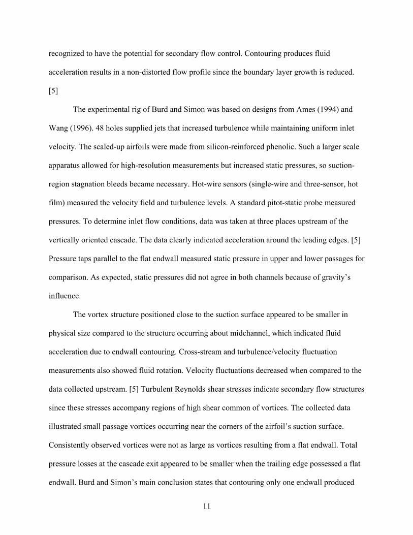
of the box in order to allow optical access of the test section. Over this hole, a large window

flange that houses a 6” diameter, 1” thick sapphire window bolts to the outside of the vessel. A

PresSure Products brand window-mounting assembly welded to the window flange houses this

big sapphire window. The window housing provides a ¼” NPT cooling air supply connection

since the sapphire window should be cooled to prolong life.

Figure 3.1.6 – Large Sapphire Window Assembly

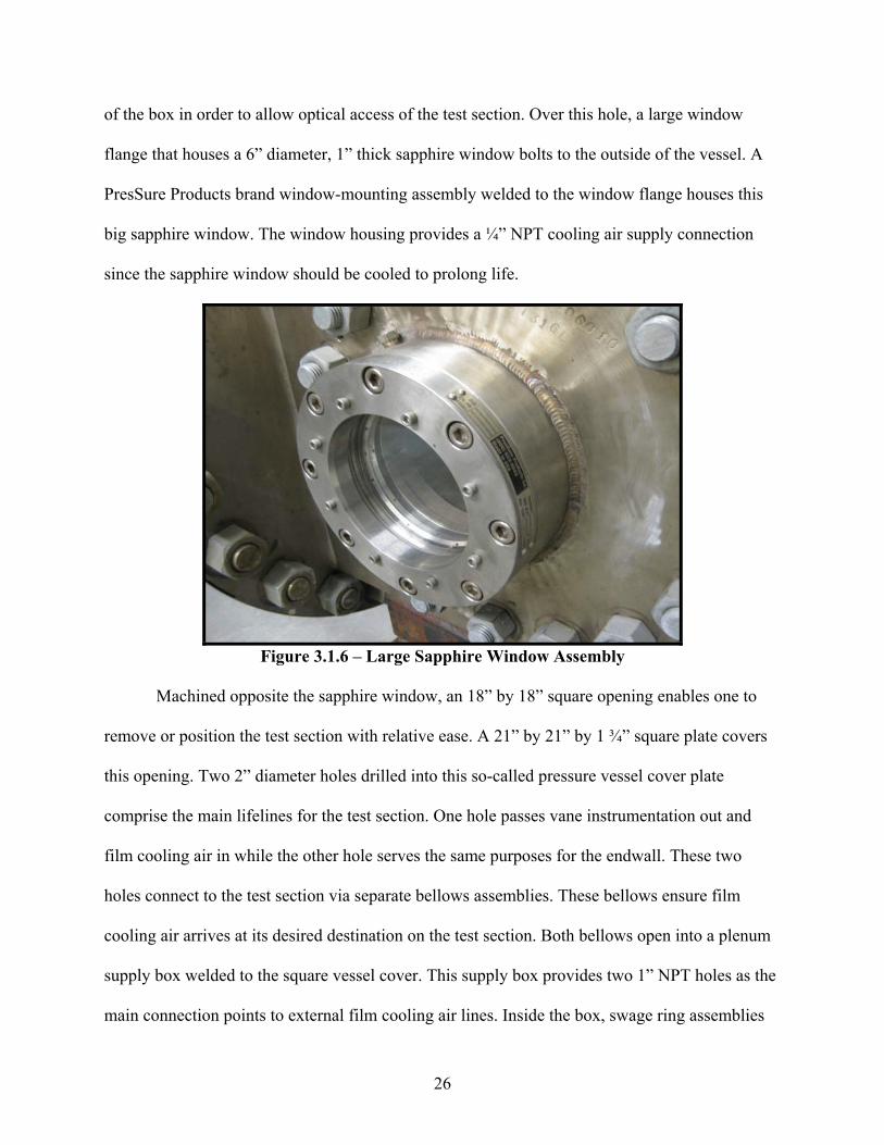
Machined opposite the sapphire window, an 18” by 18” square opening enables one to

remove or position the test section with relative ease. A 21” by 21” by 1 ¾” square plate covers

this opening. Two 2” diameter holes drilled into this so-called pressure vessel cover plate

comprise the main lifelines for the test section. One hole passes vane instrumentation out and

film cooling air in while the other hole serves the same purposes for the endwall. These two

holes connect to the test section via separate bellows assemblies. These bellows ensure film

cooling air arrives at its desired destination on the test section. Both bellows open into a plenum

supply box welded to the square vessel cover. This supply box provides two 1” NPT holes as the

main connection points to external film cooling air lines. Inside the box, swage ring assemblies

27

seal the bellows. Since the film cooling air must be pressurized, the supply box must be sealed

while still passing all instrumentation outside the vessel. A 12” by 12” by ¾” plate with six, 1”

NPT holes bolts to and seals the plenum supply box. Conax DSPG sealing gland assemblies

connect to some of the 1” NPT holes via some stainless steel pipe fittings.

Figure 3.1.7 – Cover Plate, Supply Box, and Conax Glands

These glands seal the 1/16” outer diameter stainless steel tubes housing each piece of test section

instrumentation. Further information on these sealing glands may be found in Appendix A.

However, no instrumentation initially existed to measure film cooling air temperature and

pressure close to the test section, a deficiency that called many early results into question.

To meet this need, the bellows assemblies shown in figures 3.1.9 through 3.1.11 have

been redesigned so that pressure taps and thermocouples can be located inside the test section.

This design models the functionality of a standard mechanical union used in pipe fitting.

Fabricated from 304 grade stainless steel, the two assemblies each have three pieces: an adapter

with a pocket for a bellows flange and external threads, the bellows flange, and the outer

coupling with internal threads. The adapter and coupling pieces have grooves machined in them

such that ⅛” square graphite packing seals the components. These assemblies connect to the test

Vane Plenum FC Supply

Conax DSPG Sealing Glands

Cover Plate

Plenum Supply Box with Sealing Plate

EW Plenum FC Supply

28

section in the same manner that the bellows did. Separate film cooling instrumentation fixtures

appear on the adapter pieces. Mounted via the fixtures, thermocouples have been located inside

the vane and endwall cavities, and pressure taps appear just inches away from this same area.

Figure 3.1.8 – Improved Bellows Assembly Parts

Figure 3.1.9 – Installed Bellows Assemblies before Retrofit

Outer Couplings Adapters

Bellows Flanges

⅛” Square Graphite Packing

29

Figure 3.1.10 – New Bellows Assemblies

Figure 3.1.11 – Adapter Piece Close-up

The final part of the vessel has been fabricated from a section of 24” NPS stainless steel

pipe welded to a 24” NPS cap. This third part bolts to the middle section via a matching 24”

NPS, class 300 flange welded to the pipe. Two, 4 ½” diameter exhaust holes have been machined

into the cap. After passing through the test section, exhaust gases flow out of the pressure vessel

through one of the 4” NPS pipes welded to the cap at its aforementioned openings. Like all other

flanges on this vessel, the main exhaust pipe flange has a pressure rating of 300 psig. Another 4”

exhaust pipe with a class 300 flange has been welded to the other hole in the cap at an angle of

60 degrees with the horizontal. Together with a Fike burst disk assembly, this secondary exhaust

functions as an emergency pressure relief system. Typically made from thin sheet metal pressed

into a hemispherical form, burst disks rupture in the event of excessive pressure. This assembly

simply sandwiches between two class 300 flanges even though the disks used here have a burst

pressure at just around 100 psig. Initially, water quenching would cool exhaust gases to an

acceptable temperature. A spray ring had been designed and fabricated for this very purpose. A

Thermocouple

⅛” Pressure Tap

Bellows

30

2” NPT threaded outlet on the side of the vessel provided the connection point between the water

supply and the spray ring. A 1” NPT threaded outlet on the bottom of this part of the vessel had

Figure 3.1.12 – Third Section of the Pressure Vessel with Fike Burst Disk Assembly

Figure 3.1.13 – Installed Burst Disk Assembly

the function of draining excess water. However, water quenching has since been deemed

superfluous, so the 2” and 1” NPT outlets can be utilized to pass more instrumentation out of the

vessel. This concludes all of the pressure vessel ins and outs.

31

3.1.2 Combustor and Fuel Control System

The combustor and its fuel control system round out the major equipment category.

Designed and fabricated by Stahl-Farrier Inc., this nearly nine foot long, 304-grade stainless steel

vessel can heat air to a maximum temperature of around 1000 ºF (538 ºC). A Zephyr model 4988

burner acts as core of the combustor. This burner has a maximum heat rate of 4x106 BTU/hr,

which translates into maximum fuel consumption between 3500 and 4500 SCFH (99.109 m3/hr

and 113.267 m3/hr) with natural gas as the fuel. [11]

Figure 3.1.14 – Real Life Combustor Fabricated by Stahl Inc.

32

The simple diffusion flame, nozzle-mix design of this burner creates realistic turbulence

levels. Fuel enters the burner perpendicularly to the main air that flows coaxially with the

combustor’s centerline.

A few inlets and outlets exist on this combustor. As shown in figure 3.1.14, three vessel

sections comprise this piece of equipment. All combustor vessel parts have been designed and

fabricated to meet ASME pressure vessel requirements for 150 psig of air pressure. Appendix B

gives a detailed engineering drawing (33768). Main air enters the combustor at a 6” NPS, class

150 flange welded to a pipe attached to the so-called inlet head, which consists of nothing more

than a 24” NPS ellipsoidal cap welded to a short pipe section with a 24” NPS, class 150 flange.

A deflector plate welded to the inside of cap focuses the main air flow.

The second section houses the burner as well as provides all connections to it. This so-

called inlet shell has a flat ¼” thick, 304 grade stainless steel plate rolled into a 24” diameter and

then welded to two 24” NPS, class 150 flanges. Support bars welded inside brace and secure the

burner in the combustor. A 1 ½” NPT outlet at the top supplies the main fuel to the burner

through a customized 1” NPS pipe welded to a 1 ½” NPT bushing. Next to this outlet, a ⅜” NPT

outlet gives pressure feedback from the burner. Similar to the main gas supply, the pilot flame

supply assembly connects to a 1” NPT outlet located on the side. A small sightglass has been

connected to another 1” NPT outlet found right next to the pilot flame supply. The other side of

the inlet shell has a 1 ½” NPT outlet used to connect a spark plug to the burner. Right next to

that, a 1” NPT outlet gives optical access needed for a flame scanner system.

The final section of the combustor, called the outlet shell, comprises a majority of the

combustor’s length. This long section has been fabricated from ¼” thick, 304 stainless steel plate

rolled into a 24” outer diameter tube. One end of this tube has a 24” NPS, class 150 flange

33

welded to it while a 24” NPS ellipsoidal head has been welded to the other end. A 6 ⅝” diameter

hole has been machined into the head so that a short length of 6” NPS pipe can be welded to it.

Figure 3.1.15 – Combustor Inlet Shell (view from above)

In order to make the connection to the test section’s pressure vessel discussed in the previous

section, a 6” NPS, class 300 flange has been welded to the short length of 6” NPS pipe. A shell

lining encloses ceramic blanket insulation inside the outer shell, which allows one to touch the

combustor during operation and also minimizes heat loss along the length. Mounted on a ¼”

NPT outlet welded to the exhaust 6” NPS pipe, a single type-K thermocouple measures exhaust

gas temperature. A setpoint temperature can be enacted by the control system, which can operate

in closed-loop mode using this thermocouple as an input. However, most tests do not require this

amount of control since the main air flow rate can be reliably maintained.

Appendix B shows a schematic (33767) of the fuel control system drawn by Stahl.

Natural gas enters the fuel control system via a ¾” NPT bronze ball valve. Next, a Fisher type

34

627R regulator reduces the gas pressure to 90 psig. This regulator connects to a ¾” NPS vent

line that exhausts gas in the event of overpressure. An Ashcroft pressure switch prevents system

operation in the event of high gas pressure. Made from ½” outer diameter tubing, a bleed line

located on the stem of this pressure switch sends gas downstream that lights the pilot flame. An

ASCO solenoid valve on this bleed line must open in order to light the pilot. The pilot flame gas

can be switched off by closing a leak check ball valve. Pilot flame gas undergoes one last

throttling at a ball-cock valve located right outside the combustor.

Figure 3.1.16 – Bottom Section of Fuel Control System

Next for the main gas, a set of Inline brand pneumatically actuated fuel shut-off valves trap a

certain volume of gas. These valves get pneumatic actuation from ASCO solenoid coils. The gas

in the small section should not trip another Ashcroft pressure switch set to protect the system

from a low fire condition. If gas arrives at too low a pressure, it exhausts through another ¾”

NPS vent line opened by an ASCO solenoid valve. Next, the main gas undergoes automatic

35

pressure regulation via two Jordan differential pressure regulators (Mark 63 and Mark 64). These

regulators have been set to maintain certain differential pressures across their diaphragms. The

first regulator maintains about 8 psid between the main gas and pressure in the burner supplied

by the ⅜” NPT outlet on the combustor. After the first regulator, the pipe size increases from ¾”

NPS to 1” NPS. The second regulator keeps about 1 psid between the inlet and outlet of the main

fuel control valve located a little further downstream. A Siemens 7MF4433 differential pressure

transmitter can be set up to read the gas pressure differential between the burner and before or

after the second Jordan valve. Finally and most importantly comes the main fuel control valve.

This Samson model 3522 pneumatically operated globe valve with proximity switches takes

current input to control open and close positions. After final control from this valve, main gas

enters the combustor through a 1” NPS flex hose.

Figure 3.1.17 – Upper Section of Fuel Control System

36

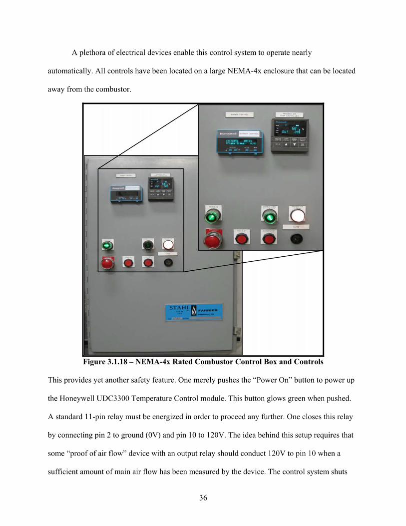
A plethora of electrical devices enable this control system to operate nearly

automatically. All controls have been located on a large NEMA-4x enclosure that can be located

away from the combustor.

Figure 3.1.18 – NEMA-4x Rated Combustor Control Box and Controls

This provides yet another safety feature. One merely pushes the “Power On” button to power up

the Honeywell UDC3300 Temperature Control module. This button glows green when pushed.

A standard 11-pin relay must be energized in order to proceed any further. One closes this relay

by connecting pin 2 to ground (0V) and pin 10 to 120V. The idea behind this setup requires that

some “proof of air flow” device with an output relay should conduct 120V to pin 10 when a

sufficient amount of main air flow has been measured by the device. The control system shuts

37

down when air flow drops below this “sufficient” level. A white “Process Air” light shines when

air flow reaches the predetermined acceptable level for combustion. The rest of the system can

operate after and only after this condition has been met. Next, one must push the “Burner

Start/System Reset” button, which also glows green when energized. This initializes

communication with a Honeywell RM7800 Burner Control unit. This unit accepts high-fire

switch, low-fire switch, and ultraviolet (UV) sensor inputs and outputs signals to an Allen-

Bradely Micrologix 1000 PLC controller. The PLC controller acts in conjunction with more 11-

pin relays to open and close the required ASCO solenoid valves located on the control system.

The burner control unit first enacts a low-fire purge that lasts for twenty seconds. Next, it does

the same for the high-fire purge. The unit then lights the pilot flame. Finally, the main flame

ignites and the unit goes into run mode. A stable 5.0V signal from a Honeywell C7035

Minipeeper UV flame scanner indicates a strong flame. This flame scanner has been located on

the previously mentioned 1” NPT outlet located on the combustor’s inlet shell. All tests should

be run once a stable flame has been achieved. Once all this equipment had been procured, the

next issue became how to adequately position a connect it all.

3.2: Facility Design and Layout

Installation of a natural gas-fired combustor requires the design and construction of

compressed air and natural gas pipelines capable of handling high pressures and flow rates.

High-temperature exhaust gases produced by the combustor need to pass through the vane

cascade. These combustion gases must then be safely vented from the lab via specially designed

and constructed exhaust pipelines. The following sections describe the main pipelines designed

and constructed to meet all these requirements.

38

3.2.1 Inlet Air

Just like a real gas turbine engine, this entire facility requires compressed air for

producing combustion gases that flow through the vane passages, for air flow through film

cooling holes on the vane and endwall, and for any air-powered devices such as control valves.

Two Atlas CopCo model GA-315 compressors have been installed outside of the lab in order to

supply enough air to cover the wide range of test conditions. Each compressor generates a

maximum of 1399 SCFM (39.6 m3/min) of air at 157 psig (10.8 barg). This means both

compressors can instantaneously together produce a maximum of 3.562 lbm/s (1.615 kg/s).

These compressors operate at 50 hp on 480V, three-phase power.

Figure 3.2.1 – Compressors, Dryers, and Tank Behind the Lab

Receiving Tank

Zander KN-32 Air Dryers

Atlas CopCo GA-315 Compressors

Main Air Pipeline to Lab

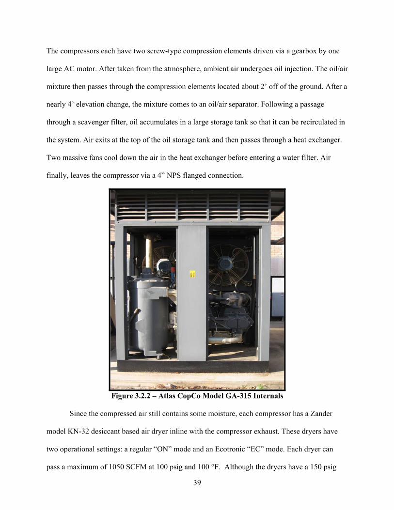
39

The compressors each have two screw-type compression elements driven via a gearbox by one

large AC motor. After taken from the atmosphere, ambient air undergoes oil injection. The oil/air

mixture then passes through the compression elements located about 2’ off of the ground. After a

nearly 4’ elevation change, the mixture comes to an oil/air separator. Following a passage

through a scavenger filter, oil accumulates in a large storage tank so that it can be recirculated in

the system. Air exits at the top of the oil storage tank and then passes through a heat exchanger.

Two massive fans cool down the air in the heat exchanger before entering a water filter. Air

finally, leaves the compressor via a 4” NPS flanged connection.

Figure 3.2.2 – Atlas CopCo Model GA-315 Internals

Since the compressed air still contains some moisture, each compressor has a Zander

model KN-32 desiccant based air dryer inline with the compressor exhaust. These dryers have

two operational settings: a regular “ON” mode and an Ecotronic “EC” mode. Each dryer can

pass a maximum of 1050 SCFM at 100 psig and 100 °F. Although the dryers have a 150 psig

40

maximum inlet pressure rating, a quoted 1590 SCFM of air can be passed through at 140 psig

and 100 °F. [12] This flow rating indicates that the compressors and dryers have been well

matched. The dryers feed both 4” NPS air lines to an accumulation tank. This massive upright

receiving tank has a capacity of 2560 gallons (11.3 m3). Air in the tank cools down to near

ambient temperature. Using a simple unsteady mass balance for air at 135 psig and 60°F, the

tank gives about four minutes of air at a flow rate of 4 lbm/s before the compressors must unload

into the tank. Two main 6” NPS ports with manual operated butterfly valves serve as this tank’s

exhausts. One of these pipelines exclusively connects the receiving tank to the hot cascade lab

because of the high flow rate requirements needed for tests.

Figure 3.2.3 – Zander Model KN-32 Air Dryers and Their Control Panels

The single 6” NPS compressed air pipeline entering the lab terminates with another

manual butterfly valve. Numerous pipeline designs have been considered in order to connect

41

downstream equipment to the main pipeline while recognizing constraints imposed by the

physical lab space. One design had even been fabricated and later determined not to be

compatible with lab equipment. All inlet air pipeline designs call for flanges and fittings adherent

to ASME B16.9 and for pipe runs to be constructed from standard A36 seam-welded carbon steel

pipe. The combustor inlet has a matching 6” NPS flange rated for 150 psig, which might cause

one to desire a straight 6” NPS pipe run from the butterfly valve to the combustor inlet.

However, the air line must be reduced to 3” NPS with class 150 flanges so that a Fisher

model ED globe valve can be connected inline in order to control main air flow. A Fisher type

667 diaphragm actuator drives this globe valve. As with all diaphragm style actuators, air must

be fed into the actuator casing to overcome the internal spring force acting on the diaphragm.

Figure 3.2.4 – Inlet Fisher Globe Valve with Diaphragm Actuator and Valve Controller

The spring inside the casing closes the valve when air has evacuated the casing. Supply air can

come from any source not downstream on the same pipeline as the valve since this would always

keep the valve closed. To control how much air enters the actuator casing, a Fisher FIELDVUE

DVC6000 series digital valve controller has been affixed to the valve. This controller requires an

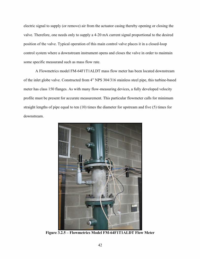
42

electric signal to supply (or remove) air from the actuator casing thereby opening or closing the

valve. Therefore, one needs only to supply a 4-20 mA current signal proportional to the desired

position of the valve. Typical operation of this main control valve places it in a closed-loop

control system where a downstream instrument opens and closes the valve in order to maintain

some specific measurand such as mass flow rate.

A Flowmetrics model FM-64F1T1ALDT mass flow meter has been located downstream

of the inlet globe valve. Constructed from 4” NPS 304/316 stainless steel pipe, this turbine-based

meter has class 150 flanges. As with many flow-measuring devices, a fully developed velocity

profile must be present for accurate measurement. This particular flowmeter calls for minimum

straight lengths of pipe equal to ten (10) times the diameter for upstream and five (5) times for

downstream.

Figure 3.2.5 – Flowmetrics Model FM-64F1T1ALDT Flow Meter

43

The above constraint severely limited pipeline design options given the amount of floor space

present to fit all equipment. Some 1” NPT outlets immediately upstream and downstream of the

flow meter can be used as measuring points for temperature and pressure For a 4” NPS inner

diameter of 4.026”, the total straight length of upstream pipe required becomes 40” or about 3.5’.

Running the straight length in plane and at right angles with the combustor/pressure vessel

centerline would not fit in the lab as some of the presented designs show. A 6” NPS long radius

(LR) elbow had been shipped with all other equipment so that the straight length could

potentially be made up still horizontal but perpendicular to the rest of the equipment.. This

configuration still did not leave much maneuvering room on the lab floor. The third design gave

more total floor space at a number of bends cost.

Figure 3.2.6 – Early Floor Plan Schematic

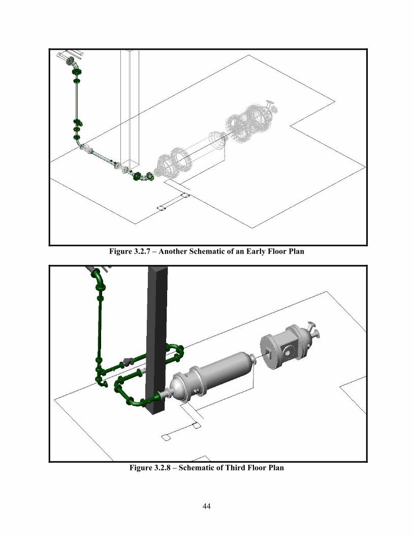
44

Figure 3.2.7 – Another Schematic of an Early Floor Plan

Figure 3.2.8 – Schematic of Third Floor Plan

45

After fabrication, errors in specifying class 300 flanges rendered this third pipeline design

unusable. A colleague finally suggested completely clearing the floor space and running the inlet

air pipeline close to the ceiling. Assembly concerns such as globe valve positioning originally

put the pipeline close to the floor. If one must service the valve inline or take it out of line, he or

she would have an easier job if the valve were located closer to the ground. At the cost of

locating the valve nearly 13’ in the air, the final pipeline design minimizes the bend count to four

and, most importantly, clears the floor space for plenty of movement around the lab.

Figure 3.2.9 – Final Inlet Air Line Design Schematic

Even though the pipe section entering the lab can safely support more than 500 lbf of weight

without yielding and without even deflecting, a couple of pipe sections and the inlet globe valve

have been anchored to the ceiling for added safety.

46

Figure 3.2.10 – Inlet Air Pipeline

A stainless steel expansion joint further embellishes the pipeline. The expansion joint

handles pipeline movement due to vibrations, thermal expansion, or equipment movement.

Positioning of this joint underwent a couple iterations. Originally, the joint had been put inline

47

with the combustor. This position has been deemed unacceptable since a misaligned expansion

joint under direct axial compression could fail due to fatigue cycling. Therefore, the 4” NPS joint

has been located perpendicular to the combustor centerline so that any movement causes a more

tolerable tensile rotational moment on the joint.

The ability to supply film cooling air imposes the final constraint on the inlet air pipeline.

Shown in the picture of the fabricated pipeline, a 6” NPS tee appears directly upstream of the

inlet Fisher globe valve. Thoroughly discussed later on in this chapter, the film cooling air line

has been designed to make use of this tee. As a final note, a few threaded outlets appear on the

main inlet air pipeline. A ½” NPT outlet goes to the combustor fuel control system to power its

control valve and regulators. One of two 1” NPT outlets has been used to supply air to the inlet

globe valve actuator. The other outlet connects to an “auxiliary” 1” NPS pipeline that runs across

the length of the lab.

Figure 3.2.11 – Stainless Steel Tube Window Cooling Assembly inside Pressure Vessel

This line has a couple of necessary functions including providing a ½” NPS air line close to the

pressure vessel. At the present, this ½” line has been setup mainly for sapphire window cooling

needs. Cooling the sapphire windows increases the life of these windows, which, in turn,

48

maximizes window life and minimizes costs. One of the 1 ½” NPT holes in the middle section of

the pressure vessel has been chosen as the connection point for a ½” outer diameter stainless

steel tube assembly with impingement holes fabricated for supplying cooling air to the sapphire

windows located on the test section as shown in section 3.1.1.

Figure 3.2.12 – Outside Sapphire Window Cooling Air Supply Pipelines

This design consists of a ½” NPS pipe welded to a 1 ½” NPT bushing that connects to the

corresponding aforementioned hole in the pressure vessel. The ½” pipe terminates inside the

vessel with a Swagelok NPT to tube union fitting connecting to the fabricated ½” tube assembly.

This ½” pipe connects to the outside auxiliary ½” NPS pipeline through a couple of Apollo ball

and check valves. The 6” diameter sapphire window on the outside of the vessel also benefits

from cooling. Embedded in the window mounting flange, an impingement ring gets its air supply

from a ¼” NPT hole on the mounting flange. A series of ¼” NPS pipe fittings connects this ring

to the same auxiliary ½” NPS pipeline used for the internal windows.

49

3.2.2 Natural Gas

As previously stated, natural gas has been designated as the combustor’s current

operating fuel. However, some initial confusion existed as to the actual natural gas requirements

for this lab. The natural gas line supplying the lab comes directly from a tie-in point located at

the LSU power plant. The university’s supplier delivers gas at 450 psig, which far exceeds the

needs of this lab and possesses many safety concerns. Running a 100’ long section of pipe

containing 450 psig of natural gas from the power plant to the connection point outside the lab

can potentially be very hazardous. ASME has many regulations regarding this type of gas

transmission. LSU facility has observed these regulations in the fabricated pipeline that delivers

the high-pressure natural gas over the long distance to the location outside of the lab.

Figure 3.2.13 – Natural Gas Pipeline outside the Lab

At the beginning of the outside equipment, a manual on-off globe valve connects to the

gas line coming out of the ground. To give a rough measure of gas consumption, a volumetric

flow meter comes right after the globe valve. Next, a Fisher BigJoe regulator reduces gas

pressure from 450 psig to around 200 psig. Finally, a Fisher Type 627R regulator with 3/16”

50

diameter orifice and internal relief reduces gas pressure from 200 psig to around a desired 95

psig needed for the combustor. The 1 ½” NPS gas pipeline runs a distance before terminating at

an Apollo ball valve located inside the lab.

Figure 3.2.14 – Fuel Control System Standing beside Combustor

Per Stahl-Farrier’s specifications of 5000 SCFH at 90 psig, a pipeline had to be designed

in order to connect the combustor control system to the main 1 ½” NPS supply line ending with

the aforementioned ball valve. A ¾” NPS brass ball valve makes up the gas inlet to the

combustor control system. The installed pipeline that connects these two ball valves reduces the

pipe sizes from 1 ½” to 1” and finally to ¾”. One spatial constraint came in the form of a

drainage pipe hung near the ceiling of the lab. This drainage pipe prevented a simple straight

horizontal run from the 1 ½” ball valve. Two 45° elbow fittings elevate the natural gas pipeline

sufficiently so it clears the drainage pipe. To minimize errors and conflicts in positioning near

the control system, a 3’ long ¾” NPS stainless steel flex hose connects the control system to the

51

pipeline. Most all fittings used here have been made from cast malleable iron (M.I.) and rated for

300 psig. All pipe runs meet ASME standards for schedule 40 seam-welded piping. Furthermore,

LSU Facility Services performed the actual installation of this pipeline because of safety

concerns associated with high-pressure gas pipelines. Facility Services also ran a couple ¾”

copper vent lines that connect two vents on the control system to the ambient air outside the lab.

Figure 3.2.15 – Natural Gas Pipeline inside Lab and Connected to Fuel Control System

3.2.3 Exhaust

Following the design and installation of the inlet air pipeline, the exhaust lines underwent

a few design iterations. Accurate exhaust line design could occur only after the pressure vessel

Drainage Pipe Obstruction

Gas Line to Fuel Control System

Gas Line Inlet to Lab

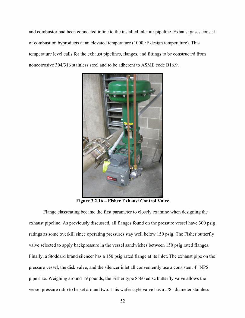
52

and combustor had been connected inline to the installed inlet air pipeline. Exhaust gases consist

of combustion byproducts at an elevated temperature (1000 °F design temperature). This

temperature level calls for the exhaust pipelines, flanges, and fittings to be constructed from

noncorrosive 304/316 stainless steel and to be adherent to ASME code B16.9.

Figure 3.2.16 – Fisher Exhaust Control Valve

Flange class/rating became the first parameter to closely examine when designing the

exhaust pipeline. As previously discussed, all flanges found on the pressure vessel have 300 psig

ratings as some overkill since operating pressures stay well below 150 psig. The Fisher butterfly

valve selected to apply backpressure in the vessel sandwiches between 150 psig rated flanges.

Finally, a Stoddard brand silencer has a 150 psig rated flange at its inlet. The exhaust pipe on the

pressure vessel, the disk valve, and the silencer inlet all conveniently use a consistent 4” NPS

pipe size. Weighing around 19 pounds, the Fisher type 8560 edisc butterfly valve allows the

vessel pressure ratio to be set around two. This wafer style valve has a 5/8” diameter stainless

53

steel shaft driven by a Fisher type 1051, size 40 rotary actuator. This actuator weighs around 95

pounds, so manually lifting the entire valve assembly does not come very easily. Like the type

667 actuators, the 1051 actuator requires pneumatic input since it possesses a diaphragm. The

same Fisher FIELDVUE DVC6000 series digital valve controller as found on the inlet valve may

be seen attached to the 1051 actuator. Again, some air source with consistent positive pressure

must be present to control this valve. The previously discussed auxiliary air line spanning the

lab’s length gives this valve its pneumatic supply. Although not yet enacted, the exhaust valve

can be part of a closed-loop control system that maintains a specific vessel/vane passage pressure

ratio by outputting a 4-20 mA current signal to the DVC6000 unit.

Figure 3.2.17 – Schematic of Main Exhaust Line with Valve

The main exhaust pipeline serves strictly to route combustion gases from the pressure

vessel to the Stoddard silencer to exit the lab. No elaborate design has been incorporated here.

The only concerns to location came in where to position the exhaust valve and in dropping the

elevation so that one can easily step over the pipeline in order get to the vessel’s instrumentation

side. The current design places the exit valve about 2’ from the pressure vessel exit flange.

54

Locating this valve too far away results in slower system response when trying to set a desired

backpressure.

As mentioned in section 3.1.2, the pressure vessel has an emergency exhaust that must

also be vented outside the lab. Design of this pipeline started with considerations to the Fike

burst assembly. A typical burst disk consists of nothing more than a piece of hemispherical-

formed metal made from very thin stock (~ 0.03125” thick). When a sufficient pressure

difference develops across this “membrane,” it ruptures analogously to an electric fuse melting

under sufficient voltage difference. The hemispherical profile gives a somewhat reliable

differential pressure rating due to minimal stress concentrations. A Fike burst disk used in this

lab has a rupture pressure differential of 100 psid.

Figure 3.2.18 – A Fike Burst Disk

This assembly must be located at the immediate exit of the 60° line coming out of the

pressure vessel to avoid any lag in pressure relief. The design question then became how to route

a pipeline that vents this line to the exhaust leaving the lab while maintaining a pressure

difference below the burst pressure during normal operation. As seen below, the first design ran

55

this emergency pipeline to a tee coming off of the main exhaust line. Benefits of this design

included easier assembly and lower cost for running a shorter pipeline.

Figure 3.2.19 – Early Floor Plan Schematic with Short Emergency Line

When analyzed closer, this idea did not seem to meet the required response time. In the event of

a failed exhaust valve, pressure may still be present at the proposed branch point since the

exhaust gases still must pass through the silencer before coming roughly to atmospheric pressure.

This would probably take an unacceptable amount of time to occur.

The fabricated emergency pipeline design connects the pressure vessel directly to the 10”

NPS silencer exit pipe. Pressure should be at or around atmospheric when exiting the silencer.

For the required burst pressure of 100 psid, this design gives a safe means for emergency

pressure relief. However, no tie-in point initially existed on the pipeline ran from the silencer to

the outside of the lab. This 10” NPS schedule 10 pipeline had to be taken down and have a 4”

NPS flanged connection point attached.

56

Figure 3.2.20 – Schematic of Fabricated Exhaust Lines

The final fabricated exhaust pipeline provides three drains via 1” NPT threaded outlets to

remove condensed water from the pipelines. These outlets may be found on the “bottoms” of

certain pipeline sections. A 1” NPT threaded outlet located on the emergency pipeline may be

used to insert some flow detection sensor that can feed a signal to an alarm or to a controller to

shut off the system when exhaust gases flow in this line due to an open burst disk. Because this

pipe section becomes quite unwieldy due to its size and weight, the threaded outlet also doubles

as a lifting point at this section’s center of gravity. On the main pipeline section immediately

exiting the pressure vessel, ½” and 1” NPT threaded outlets can be used to insert a thermocouple

and/or a pressure sensor in order to measure the exhaust conditions. At the present, a pitot-static

probe has been inserted into the 1” outlet. Via an attached pressure gage, this probe gives a

visual measurement of exhaust gas total pressure. Comparing this pressure reading to that at the

vessel inlet yields the vessel pressure ratio.

57

Figure 3.2.21 – Exhaust Pipelines Installed in the Lab

A fully functional, natural gas burning flow loop had been adequately achieved after all three of

the pipelines discussed in this section had been installed. However, this facility’s design did not

end there.

58

3.3: Film Cooling Line Design

The focus next fell on setting up some sort of film cooling air supply pipeline. Inclusion

of this pipeline’s connection point provided a necessary constraint on the early inlet air pipeline

designs. After the inlet pipeline had been designed, fabricated, and assembled, the vertical

branch of the 6” NPS tee immediately upstream of the inlet control valve had been chosen as the

most logical tie in point for the film cooling line. Just like the main air line, 6” reduces to 3” on

the film cooling line leaving the tee. Some previously fabricated 3” NPS pipe sections utilizing

class 300 flanges from the failed inlet air pipeline design gave some preexisting materials from

which one could work. Beginning with a 3” NPS tee fitted with class 300 flanges, the film

cooling line runs perpendicular to the main air line.

Figure 3.3.1 – Schematic of Film Cooling Line Design

After a reduction in the pipe size from 3” to 2” NPS and a change in flange class to 150, a

refurbished Fisher type ED globe valve with 2”, class 150 flanges acts as this line’s main

regulator. This particular valve offered a great price for the unbeatable functionality of a Fisher

control valve just like the main inlet valve. Currently, the film cooling valve operates in a strictly

open or closed mode since more precise flow throttling occurs further downstream. After the

59

pipe size increases again to 3”NPS, a previously fabricated long pipe section terminates with a

6”, class 300 flange This pipe’s length conveniently brings the film cooling air pipeline close

enough to the pressure vessel. A 6”, class 300 blind flange with a 1 ½” NPT hole completes this

long pipe section.

Figure 3.3.2 – Actual Film Cooling Line with Fisher Globe Valve

Before any further pipelines had been designed from this 1 ½” hole, film cooling air flow

requirements had to be calculated so that the film cooling pipeline would confidently supply

sufficient air flow. Early discussions indicated that required film cooling flow requirements

would not be near the 4 to 5 lbm/s needed for the main air. The 2” pipe sections could reliably be

used knowing this information, but using any pipe sizes under 2” became a concern. However,

1” NPT holes already exist as the main film cooling air supply connection points on the pressure

vessel’s plenum supply box as detailed in section 3.1.2. The design problem then became finding

an adequate means for splitting the 1 ½” hole into pipelines that terminate with 1” NPT

connections at the pressure vessel. A parameter known as the blowing ratio became the basis for

60

calculations since knowledge of flow requirements enables one to specify film cooling pipeline

instrumentation and hardware.

Blowing ratio, M, appears almost exclusively in discussions involving film cooling. In

gas turbine applications, a singular film cooling hole pushes a small diameter jet of air into the

bulk mainstream fluid consisting of combustion gases flowing crosswise (non-parallel) to that

jet. This parameter expresses the ratio of mass rate flux of the jet to the mass rate flux of

crossflow.

ρ V jetM =ρ V cross

For convenience, many in the gas turbine field also use a momentum flux ratio, I, defined in

much the same way:

2ρ VjetI =

2ρ Vcross

One can clearly see that a velocity ratio, VR, relates the two parameters:

VjetI = M VR where VR =Vcross

However, only the blowing ratio has been considered for these rough calculations.

One can calculate how much film cooling air needs to be supplied by using the blowing

ratio definition. A range of blowing ratios from around 0.5 to around 2 has been specified as a

desired test condition set. Also, the test sections used in this facility have been designed for use

with about 4 to 5 lbm/s of mainstream air. By using the definition of mass flow rate, one can find

61

the mass rate flux of crossflow by dividing the operating mass flow rate by an appropriate area

term designated as Across:

&mcrossρ V =cross Across

An accurate Across used for this estimation has been selected as the cross-sectional area of the

passage immediately upstream of the test section. The numerical value of this area has been

taken from solid models used to fabricate the test sections. The mass flow rate of film cooling air

can be found in a similar way with a few simplifying assumptions. If one assumes that film

cooling air flows equally through each film cooling hole, then the total film cooling mass flow

rate equals the summation of all jet mass flows:

& & &nh

m = m = n mjetFC, total jet, i hi

Now assuming equal cross-sectional area of each hole (all film cooling holes get their shape

from a 0.03” diameter dill bit):

&m = n A ρ VFC, total h h jet

All of these equations can be combined to form one expression for estimating total film cooling

air required:

& &Ahm = n m McrossFC, total h Across

Since the number of film cooling holes varies between the vane and endwalls as discussed in

section 3.1.1, different amounts of film cooling air require two separate pipelines in order to

maintain similar a blowing ratio between vane and endwall. The following plot summarizes the

requirements.

62

Figure 3.3.3 – Estimated Film Cooling Requirements for Endwall and Vane

These estimates show that in order to test blowing ratios up to three at a crossflow mass flow of

5 lbm/s, the vane film cooling line should be able to supply about 0.05 lbm/s of room

temperature air while the endwall line should supply about 0.02 lbm/s.

Figure 3.3.4 – Estimated Film Cooling Requirements for the Upstream Contour Section

Not to be forgotten, the 52 film cooling holes located on the upstream contour of the test section

must also be supplied with film cooling air. Using the same equation as above, film cooling air

requirements for the upstream contour section has the graph shown in figure 3.3.4. One can

63

observe that these requirements nearly equal those for the endwall. This upstream contour

section has a sealed plenum under the holes much like the inner endwall. The plenum has a

37/64” diameter hole drilled through the side for ⅜” NPS threads to be formed. However, a ⅜”

NPS line cannot be run through the same space occupied by the instrumentation/main film

cooling bellows. One of the few feasible options left routes the ⅜” line through one of the two 1

½” NPT holes located on the bottom of the pressure vessel. Some thought must be put into

physical assembly of this pipeline since the inside of the pressure vessel does not leave much

room to adequately tighten pipelines with large pipe wrenches. Keeping this air line at ⅜” creates

negligible pressure drop as long as its main connection point does not lie too far away.

Figure 3.3.5 – Upstream Contour Supply Line inside Pressure Vessel

As shown in figure 3.3.5, the enacted design uses a couple ⅜” NPS mechanical unions rated for

150 psig since they fit inside the 1.610” inner diameter of 1 ½” NPS sch40 pipes. This solution

runs the ⅜” line (with unions) out of the vessel via a specially fabricated 1 ½” NPT bushing

fitted with a ⅜” NPS nipple connecting to a reducer that increases pipe size to ½”. Seen in figure

64

3.3.6, the now ½” NPS line terminates with a manual needle valve that gives precision flow

control through this line.

Figure 3.3.6 – Upstream Contour Needle Valve

Via a tee on the endwall film cooling line, incorporation of the upstream contour air line into this

line makes film cooling air requirements near equal for the vane and endwall lines. Both cooling

lines, therefore, must be capable of supplying about 0.05 lbm/s of air. According to these rough

calculations, running experiments up to a blowing ratio of about three requires only 0.1 lbm/s of

cooling air from the main air line. With this in mind, two nearly identical 1” NPS cooling air

lines can confidently be designed and installed for this application. If a 4” pipeline can

comfortably pass 5 lbm/s of air, then a 1” line must be able to pass a hundredth of that flow.

These two lines should originate from a split shortly downstream of the 1 ½” NPT hole

mentioned earlier. The experimenter should have the means to finely tune flow in the two lines

via 1” NPS precision needle valves. In addition, these cooling lines should posses accurate and

65

reliable flow instrumentation since knowing how much air flows through the film cooling holes

allows one to compute a blowing ratio. Numerous designs for these lines have been constructed,

but the final configuration appearing in section 3.4 gives the best functionality.

Another desired experimental embellishment presents even more issues. Heating the film

cooling air changes the system’s density ratio (density of cooling air jet divided by density of

crossflow). Using the ideal gas law, density ratio has the following definition:

Pjet

ρ R T P RTjet jet cgasairjet crossDR = = =ρcross Pcross P T Rcross jet airR Tcgas cross

The gas constant for combustion gases, Rcgas, cannot exactly be provided numerically, so this

value should be assumed to be very close to the gas constant for air, Rar. Although the static

pressure of the jet must be slightly higher than that of the surrounding crossflow, one can assume

here that the two static pressures nearly equal each other, which produces an absolute pressure

ratio typically between 1.0 and 1.1. The temperature ratio, therefore, provides the true driving

factor in the density ratio equation. Since combustion gases pass through the cascade at a design

temperature of 1000 °F, a temperature range for film cooling air between room temperature and

500 °F yields a temperature ratio (and density ratio) range from 2.75 to around 1.5. The next

issue becomes how to adequately incorporate this flexibility in the two main film cooling lines.

A few air-heating methods such as circulating hot combustion gases in a heat exchanger

have been considered for this application. However, a simple electric heater seems to beat all

other options when feasibility becomes paramount. A control volume analysis gives an

expression for the amount of power input required to heat room temperature air to 500 °F.

66

& && &2 2V Vinlet exitQ +m h + =W +m h +loss inlet inlet in exit exit2 2

Assuming steady state with negligible heat loss to the environment, this equation reduces to:

&& &

m R T1 2 2 airW =m h - h + V - V and V=ein i i e2 A P

Finally, substituting an expression for enthalpy of air and an expression for velocity derived from

the continuity equation and ideal gas law gives:

&& &

222R TT3m air eiW =m c T - c T + -in p, i i p,e e A P P2 i e

This equation can be simplified if pressure loss across the heating length can be neglected, but

this formula contains enough known variables to assign nominal values. The internal area, A, has

been taken as the area of a circle with diameter equal to 1.049” (the internal diameter of 1” NPS,

schedule 40 pipe). The following graph shows the power required to heat room temperature air to

500 °F at a constant nominal pressure of 100 psig.

Figure 3.3.7 – Power Estimates for Film Cooling Air Heater

67

The nearly 12kW of power needed to heat 0.1 lbm/s of air should not be taken lightly.

Many commercial or industrial electric heaters capable of supplying this power need 240V or

480V (3 phase) circuits. Voltages in this range can be hazardous and even fatal if one does not

exercise discretion. Since exit temperature must be varied, some safe control over input voltage

must be present. Finally, location of the heater dictates what material pipe fittings can be used on

the main film cooling lines. Stainless steel pipe fittings can handle higher temperatures than

regular carbon steel fittings. Precautions must be taken so that pipelines downstream of the

heater arrangement do not burn people running the experiments. The 500 °F exit temperature

also limits many options for flow regulation and instrumentation. New ideas and considerations

alter the approach used in designing these pipelines. The next section presents the end solution.

3.4: Current Facility Layout and Operation

Figure 3.4.1 – Schematic of Current Lab Layout

This lab’s current layout pictured above maximizes floor space by running nearly every

pipeline off of the ground. Most of the electrical equipment has been connected to a “control

room” partition located in the lab. From here, two Fisher-Rosemount DPR950 controllers operate

Combustor

Main Film Cooling Line and Valve

Inlet Valve Film Cooling Lines

Pressure Vessel Exhaust Valve

Main Air Line

Silencer

Exhaust Lines

68

all three Fisher control valves. The Flowmetrics turbine-based mass flow meter came with its

own 924-ST2 flow computer that provides an interface for the flow meter. This flow computer

takes inputs from the flow meter’s sensors, which consist of a pressure sensor and a magnetic

pickup with embedded RTD. Pulses produced by the rotating turbine element register in the

magnetic pickup as voltage pulses that translate into a volumetric flow rate. Flow computations

convert static pressure, static temperature, and volumetric flow rate into a mass flow rate. The

flow computer also provides alarm relays as well as current outputs proportional to the measured

mass flow rate. A simple control loop takes one of these 4-20 mA current outputs from the flow

computer and sends the signal to one DPR950 that uses PID parameters to output a proportional

4-20 mA current signal to the DVC6000 controller attached to the main inlet valve.

Figure 3.4.2 – Fisher DPR950 Controllers and Flowmetrics 924-ST2 Flow Computer

The system acts in typical closed loop fashion where one only needs to input the desired mass

flow rate setpoint into the DPR950. At the present, a mass flow rate of 4 lbm/s (1.81 kg/s) can be

maintained with little variation (+/- 0.1 lbm/s or +/- 0.045 kg/s) for as long one desires to run the

69

flow loop. The film cooling line globe valve shares a DPR950 with the main inlet valve. A

control loop need not be enacted with this valve because of the film cooling line’s complexity

downstream of the globe valve. Instead, the DPR950 simply outputs a constant current signal

that opens this valve. The exhaust valve gets its own DPR950 controller. Operating this

controller in “manual” mode allows one to set the vessel pressure ratio, PR, anywhere from one

to about five. As repeatedly stated, a pressure ratio of around two has been selected for most all

tests run in this facility. This particular pressure ratio produces the desired Mach number

distribution along the endwall and vane surfaces.

As discussed in section 3.3, the film cooling lines supplying air to the endwall and vane

plenums have undergone a couple of design iterations before deciding on their current

configurations.

Figure 3.4.3 – Actual Lab Picture Taken from Control Room

70

Coming right out of the 1 ½” NPT hole and before the pipeline splits into the two 1”

lines, a short section has been designed to provide future functionality with film cooling tests

(that include pulsed studies). The two 1” NPS lines have been built from 304 stainless steel pipe

fittings rated for 150 psig of pressure. This decision came as a result of uncertainty on where

some density ratio altering heater(s) would be positioned along these pipelines. Each of the two

lines has a Sierra 640S Thermal Mass Flow Meter. These meters offer excellent accuracy for this

particular flow metering application as discussed later on in this chapter.

After the 640S flow meters, two NOSHOK model 408 FFS 1” NPT needle valves give

precise control over the amount of air entering the endwall and vane plenums. Constructed with

EPDM o-rings and parts made from 316 stainless steel, these valves can handle temperatures up

to about 400 °F, which also became a requirement due to the confusion over heater location.

Fortunately, the needle valves cost about as much money as most bronze needle valves of the

same size and flow capacity. The final location for the heater(s) became obvious once the

Farnam-Custom HeatTorch™ 200 inline heaters had been discovered. Two units have been

procured since one heater costs only $500. Each heater can output 7kW of power and pass up to

100 SCFM of heated air. Since each heater measures only about 14” long, the best location

places them close to the pressure vessel and downstream of the needle valves. This position

eliminates concerns for potential abuse of needle valves due to excessive temperatures, possible

interference with the thermal mass flow metering process, and certain heat loss along long

lengths of uninsulated stainless steel pipe. As detailed in section 3.3, film cooling air delivered to

the upstream contour section can be regulated by a ½” NPT needle valve that connects to a tee in

the endwall supply line downstream of its heater. This film cooling line design offers a reliable

and fully functional means of measuring how much film cooling air flows into all parts of the

test section, which becomes a necessity when accurately computing a blowing ratio.

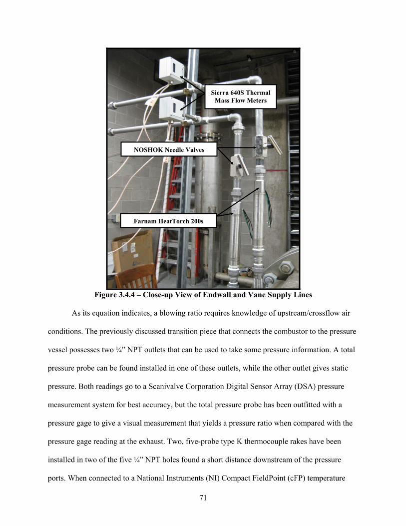
71

Figure 3.4.4 – Close-up View of Endwall and Vane Supply Lines

As its equation indicates, a blowing ratio requires knowledge of upstream/crossflow air

conditions. The previously discussed transition piece that connects the combustor to the pressure

vessel possesses two ¼” NPT outlets that can be used to take some pressure information. A total

pressure probe can be found installed in one of these outlets, while the other outlet gives static

pressure. Both readings go to a Scanivalve Corporation Digital Sensor Array (DSA) pressure

measurement system for best accuracy, but the total pressure probe has been outfitted with a

pressure gage to give a visual measurement that yields a pressure ratio when compared with the

pressure gage reading at the exhaust. Two, five-probe type K thermocouple rakes have been

installed in two of the five ¼” NPT holes found a short distance downstream of the pressure

ports. When connected to a National Instruments (NI) Compact FieldPoint (cFP) temperature

Sierra 640S Thermal Mass Flow Meters

Farnam HeatTorch 200s

NOSHOK Needle Valves

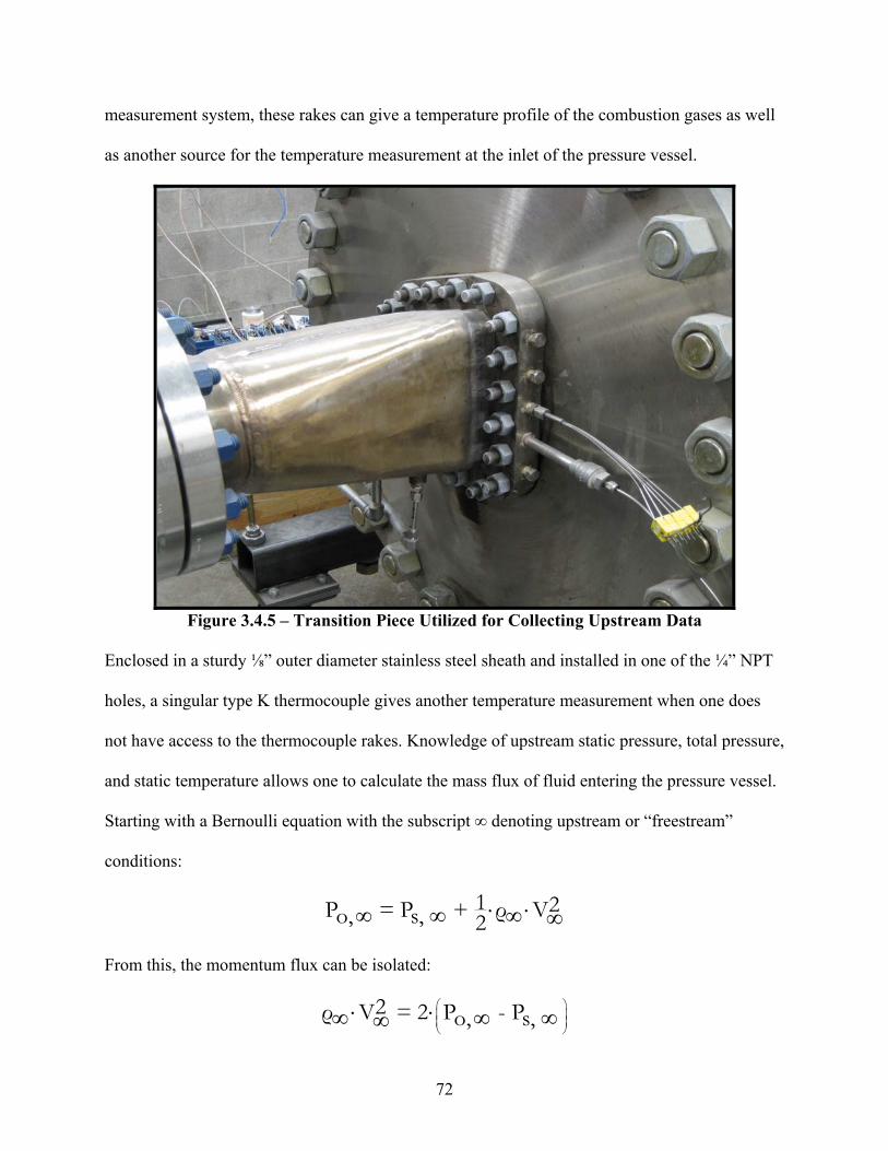
72

measurement system, these rakes can give a temperature profile of the combustion gases as well

as another source for the temperature measurement at the inlet of the pressure vessel.

Figure 3.4.5 – Transition Piece Utilized for Collecting Upstream Data

Enclosed in a sturdy ⅛” outer diameter stainless steel sheath and installed in one of the ¼” NPT

holes, a singular type K thermocouple gives another temperature measurement when one does

not have access to the thermocouple rakes. Knowledge of upstream static pressure, total pressure,

and static temperature allows one to calculate the mass flux of fluid entering the pressure vessel.

Starting with a Bernoulli equation with the subscript ∞ denoting upstream or “freestream”

conditions:

1 2P = P + ρ Vo, s, 2

From this, the momentum flux can be isolated:

2ρ V = 2 P - Po, s,

73

Multiplying both sides by the freestream density allows one to solve for the mass flux:

ρ V = 2 P - P ρo, s,

Using the conservation of mass, multiplication of this mass flux in the freestream transition piece

by an area ratio to correct for the area variation between the freestream and the test section gives

the mass flux of fluid entering the test section passages just after the upstream contoured section.

P As,2ρ V = P - Po, s,cross R AT crosss,air

The standard expression for freestream density has been substituted in the above equation, and

the technical gas constant should be that for combustion gases, Rcombustion. Presumably, Rcombustion

and Rair have nearly the same value since no other data exists. As specified by test section

drawings, values for A∞ and Across equal 40.93 in2 (264.1 cm2) and 25.51 in2 (164.6 cm2),

respectively.

A previous discussion in section 3.3 gives a guideline for finding the other component in

the blowing ratio equation. For obtaining the mass flux of the jet, one chiefly assumes that all of

the film cooling air flows equally through each film cooling hole. No instrumentation exists on

the test section that measures mass flux through each film cooling hole in order to validate or

discredit this claim. The film cooling supply lines’ accurate mass flow instrumentation allows the

jet mass flux to be expressed as:

&mFC, totalρ V =jet n Ah h

Because local flow conditions on the test section cannot be directly measured, a nominal blowing

ratio can now be defined as:

74

&ρ V mjet FC,total A1 crossM= =n A Aρ V Ps, h h2cross P -Po, s,R Ts,air

All of the instrumentation embedded in the test sections described in section 3.1.1 has

absolutely no significance without measurement systems to collect the raw data. Pressure data

coming from the 52 pressure taps found on the pressure test section enters the digital domain

through two Scanivalve Corporation model 3217 DSAs. Other DSA models can measure

absolute pressure, but these DSA 3217 units offer sixteen channels of differential pressure

measurement at +/- 100 psid (+/- 6.89 bar) full range scale. [13] Each system can be interfaced to

computer via an Ethernet connection. The DSA 3217 has a few other features such as a zero-

calibration (CALZ) command to zero out the pressure readings and an option for enabling

temperature data collection. Combined with the point pressure data, these temperatures allow the

DSA to act somewhat as a local density-measuring device.

Figure 3.4.6 – Scanivalve Model 3217 DSA and NI cFP System

A single 64-channel National Instruments (NI) Compact FieldPoint (cFP) system collects

all of the raw temperature and voltage data produced by the Medtherm heat flux gages with

75

embedded thermocouples. The cFP system consists of a cFP-BP-8 backplane that interfaces eight

input/output modules to a cFP-2000 real-time (RT) controller that allows Ethernet and serial

connectivity. This particular setup has five cFP-TC-120 thermocouple input modules and three

cFP-AI-112 analog input modules. The TC-120 module provides eight channels of thermocouple

or millivolt input; however, thermocouples must be physically wired to a cFP-CB-3 isothermal

connector block corresponding to each TC-120 module. Isothermal connector blocks minimize

thermal gradients at connection points that may affect temperature readings produced by the

thermocouples. Each TC-120 offers built-in linearization and cold-junction compensation (CJC)

for eight different thermocouple types. [14] The AI-112 modules have sixteen channels that

accept varying voltage input ranges. Other configurable settings make these modules a great

choice for measuring the small voltages produced by the Medtherm heat flux gages. [15] Similar

to the TC-120 modules, physical connections must be made to cFP-CB-1 connector blocks in

order to pass information to the AI-112 modules.

The cFP system comes with the NI Measurement and Automation Explorer (MAX)

software, which allows the user to see the system’s operation and collected data on the computer

screen. However, this program lacks a degree of flexibility when one needs to write data to a

readable file that can be processed and analyzed. The NI-developed programming language

LabVIEW expands the capabilities of many instrumentation systems including the cFP system.

The LabVIEW program written for the cFP system achieves the main objective of outputting

data to Comma Separated Variable (*.csv) files that can be read and processed by programs such

as MATLAB and Microsoft Excel. The Scanivalve system comes with its own computer

program that allows a data output file to be written in *.csv format. A LabVIEW program written

for the Scanivalve system performs the same function but makes controlling data collection

easier. Appearing in appendix C, a master LabVIEW program has been written to provide a

76

singular interface from which the cFP and Scanivalve systems can both be controlled. This

program provides real-time viewing of certain temperatures and pressures as well as a master

“Acquire Data” control when one needs to write the incoming data to a *.csv file. NI

manufactures a slew of input and output equipment that could make the entire lab controllable

essentially from one computer program written with LabVIEW.

3.5: Instrumentation and Experimental Uncertainty

Before any experimental results can be presented, a detailed uncertainty analysis must be

performed in order to inspire confidence in the data. Any geometric information (i.e. chord

length, camber length, test section inlet area) has been obtained from the original solid models

used to fabricate the test sections. Geometric errors can be assumed to be near negligible since

the fabrication processes has very tight tolerances. Therefore, the main sources of error in all

calculations come from instrumentation and their associated measurement systems. Before

continuing any further, some background information on the heat flux gages must be presented.

The Medtherm model 4H-50-36-36-20753 heat flux transducers present on the heat

transfer test section can be classified as thin-foil type sensors. Designed to operate in high

temperature environments, these sensors (also known as Gardon gages) produce a linear EMF

(voltage) output proportional to an incident heat flux at a constant foil edge temperature. [16]

The produced EMF results from the thermal gradient across the copper lead attached to the foil

edge where the foil acts as the sensor “head” exposed to the high temperature media. This

gradient enables a flow of thermal energy and a flux of electricity. Another copper lead in the

rear of the sensor head produces another measurable EMF, which when combined with the foil

edge lead EMF, generates a voltage differential proportional to the net heat flux absorbed by the

gage. A type K thermocouple attached to the foil edge allows for correction of heat flux output

77

responsivity, but more importantly, it gives the temperature of the media in contact with the

sensor.

Figure 3.5.1 – A Medtherm Model 4H-50-36-36-20753 Heat Flux Gage

The gages have a 36” long cable sheathed in 1/16” outer diameter, grade 304 stainless

steel tubing packed with Magnesium Oxide (MgO) insulation. This can withstand temperatures

up to 2100 °F, but a maximum foil edge temperature of 1600 °F should not be exceeded.

However, the sheath should be insulated from high heat fluxes. [16] Also, a more accurate and

correct heat flux reading can be obtained when the rear of the sensor head has been immersed in

some insulating material such as Cotronics’ Resbond™ 940 ceramic sealant used to bond the

gages to the heat transfer test section. Ensuring a well-insulated and well-sealed gage seems to

mitigate heat flux errors resulting from flow of hot gases past the entire gage body instead of just

to the sensing area where the hot gases need to contact. Despite many precautions, all possible

heat flux measurement errors cannot be avoided. Because stainless steel conducts heat, the gage

absorbs some heat flux coming from the test section into the sensor head through a multi-

dimensional transfer. The sensor head possesses a very small mass, so the gage becomes subject

to low thermal capacitance. No cure seems to exist for this possible fault.

78

Figure 3.5.2 – Heat Transfer Endwall Inner Plenum with Thermal Sealant

Each heat flux gage has a responsivity correction factor used when the foil edge

temperature falls between 850 and 1600 °F, but nearly all data collected here falls below this

range and does not require such a correction. Because of this, voltage readings can simply be

converted to heat fluxes, q”, by multiplication of the responsivity, k.

q" = k v

In the documentation provided, responsivity has the units of 2BTU ft s mV . [16] Appendix D

shows a typical response curve supplied by Medtherm. The error in heat flux measurement

produced by the gage, uq”, comes from this conversion.

q" q"u = u where = k fcn vvq" v vvu = k uvq"

Knowing whether one measures V or mV becomes quite important since the responsivity has

units of mV in the denominator. A similar uncertainty analysis might be extended to the

79

thermocouples, but this does not really need to be done since all thermocouples connect to the NI

cFP system, which recognizes the voltage input and automatically converts it into a temperature

using preprogrammed linearization algorithms. The error in temperature reporting comes from

the errors associated with the cFP system. To finish off this error analysis the basic

instrumentation, a pressure tap does not need any sort of error analysis because pressure comes

out of the tap without any conversion.

The basic errors associated with the main measurement systems stem mainly from

linearity and accuracy errors. The DSA 3217 has an accuracy of +/- 0.05% of the full-scale +/-

100 psid range. This unit must operate in an ambient temperature of 0 to 60 °C (32 to 140 °F) in

order to maintain a total thermal error of less than +/- 0.001% of the full scale. [13] Errors with

the cFP system come solely from the representative input modules. Documentation on the cFP-

2000 controller does not indicate any error propagation associated with this device. The cFP-CB-

1 and cFP-CB-3 connector blocks utilize cold junction compensation through a thermistor with a

typical accuracy of +/- 0.15 °C (0.3 °C maximum). [17] All cFP-TC-120 modules read this cold

junction temperature and, therefore, have the same cold junction accuracy error. In order to make

thermocouple measurements easy, the cFP-TC-120 input modules use NIST-175 linearization

algorithms that give accuracies of +/- 0.05 °C (+/- 0.03 °F) for many types of thermocouples.

[14] The chart pictured in figure 3.5.3 shows the absolute accuracy of a typical cFP-TC-120

module measuring a type J, K, N, T, or E thermocouple. Absolute accuracy consists of gain and

offset errors, differential and integral nonlinearity, quantization and noise errors, linearization

algorithm errors, and cold junction temperature measurement errors. [14]. As one can see, typical

operation produces an error at around 0.5 °C (0.9 °F). Tests in this facility can go up to a

maximum of 1000 °F (538 °C) where the maximum error does not even exceed 1.5 °C (2.7 °F).

As mentioned in section 3.4, the cFP-AI-112 modules offer eight nominal input ranges at high

80

and low filter settings. In order to most accurately measure the millivolt outputs from the heat

flux gages, the modules need to be set to the smallest nominal input range of +/- 60 mV.

Figure 3.5.3 - Absolute Accuracy Chart for the cFP-TC-120 Input Module [14]

Although these modules offer a 500 Hz filter setting, normal measurements only require a 50-60

Hz setting, which produces an effective resolution of 3 μV in the +/- 60 mV nominal input range.

[15] For this same input range, the cFP-AI-112 has a typical accuracy under normal operating

conditions (15 to 35 °C ambient temperature) of +/- 0.03% of the reading with +/- 0.05% of the

full scale (the maximum value of the nominal input range). [15] These two percentages can be

combined when considering that the maximum reading equals the maximum value of the

nominal input range. Therefore, the maximum normal typical accuracy should be +/- 0.08% of

60mV. A few other negligible errors exist with the cFP-AI-112 module that do not need to be

included due to their lack of magnitude. [15] Table 3.1 summarizes the total error for each

measurement system where this error can be computed using the standard root-sum-squares

(RSS) method applied to elementary error components provided. The cFP-AI-112 modules also

have warranted accuracies at normal conditions (15 to 35 °C ambient temperature) of +/- 0.05%

of the reading with +/- 0.3% of the full scale. [15] The total error associated with these

81

accuracies becomes +/- 0.210 mV for the +/- 60 mV nominal input range; however, the typical

accuracies presented in table 3.1 can be used instead since these modules operate in a fairly

typical environment. Some basic uncertainties in some key test parameters can now be calculated

using the above table.

Table 3.1 – Total Errors for DSA 3217 and cFP Modules

Accuracy Thermal Resolution Total Error

Scanivalve DSA 3217 0.050 psid 0.001psid --- 0.050 psid

NI cFP (TC-120 modules) 0.900 F --- --- 0.900 F

NI cFP (AI-112 modules) 60 mV; 50-60 HZ

0.048 mV --- 0.003 mV 0.048 mV

The reported quantities of pressure ratio, PR, nondimensional temperature, θ, normalized

metal temperature, φ, and heat transfer coefficient, h, all have propagated error associated with

the respective systems used to measure them. A pressure ratio of total pressure, Po, and static

pressure, Ps, has the definition:

PoPR =Ps

Both pressures must be in absolute units (psia) in order to properly define this ratio. Using the

RSS method, an expression for the uncertainty in pressure ratio can be formulated.

2 2PR PRu = u + uPR P PP Po so sP Po s

Since the Scanivalve system measures both the static pressures on the pressure test section

surfaces and the total pressure at the inlet of the vessel, the elementary errors uPo and uPs have the

same value uP, which equals the Scanivalve total error found in table 3.1. After evaluating the

82

partial derivatives, the total error in pressure ratio at any pressure tap on the test section surface

may be given by:

22 P1 ou = u + -pPR P 2s Ps

Finally, this expression simplifies to:

u 2pu = 1+ PRPR Ps

The above equation shows an obvious dependence on static pressure; lower static pressures drive

up the pressure ratio and its corresponding uncertainty. For the following data presented in

chapter 4, a maximum pressure ratio of 2.13 occurs at a static/surface pressure of around 8.7 psig

(0.6 bar). This produces a maximum uncertainty in pressure ratio of about +/- 0.014.

Similarly, an expression for the total uncertainty in nondimensional temperature, θ, starts

with the equation:

2 2Tθ θ ou = u + u where θ =θ T TT To so sT T To s s

As with all ratios, these temperatures must have absolute units (°R or K). The elementary errors

uTo and uTs both equal the error uT associated with the cFP-TC-120 input module’s total error of

0.9 °F (0.5 °C). Error in nondimensional temperature can be compacted to:

u 2Tu = 1+ θθ Ts

The maximum temperature ratio reported for heat transfer tests equals 1.17 at a static/surface

temperature of 564.75 °F (296 °C) for a maximum total uncertainty in nondimensional

temperature of about +/- 0.0037.

83

Next, normalized metal temperature, φ, quantifies how efficiently a certain amount of

film cooling air lowers the temperature of the vane/endwall surfaces thereby reducing heat

transfer into these surfaces. It has the definition:

T - Ts=T - Tc

This parameter essentially compares the difference in freestream, T∞, to static/surface, Ts,

temperatures to the difference in freestream to film cooling air, Tc, temperatures. Uncertainty in

φ can be expressed as:

2 2 2

u = u + u + uT T TT T Tc sc sT TT c s

Because the cFP-TC-120 modules measure all temperature data, each elementary error uT∞, uTc,

and uTs equals the error uT found in table 3.1. After evaluating partial derivatives and some

rearranging, the uncertainty becomes:

2 22T - T T - T-1c s su = u + +T 2 2

T - TT - T T - Tcc c

Bringing the common denominator outside the square root simplifies this to:

2u 2 T - Tc sTu = 1+ +T - T T - Tc c

One can observe a strong dependence on the difference between freestream and coolant

temperatures. This seems to indicate some dependency on density ratio. As the difference

between coolant and freestream temperatures becomes smaller, the uncertainty in φ increases.

84

This condition corresponds to density ratios approaching one. For test cases conducted, the

thermocouples at the leading edge of the heat transfer vane produced the maximum uncertainty

in φ of +/- 0.003.

Finally and most importantly, the concept of a heat transfer coefficient, h, comes from

Newton’s Law of Cooling. Such a coefficient has the definition:

q"h =

T - Ts

Uncertainty for this key parameter can be found by starting with:

2 2 2h h hu = u + u + uh T T q"T T q"ss T q"T s

Again, the elementary errors uT∞ and uTs both equal the error uT because the cFP-TC-120

modules measure all temperatures. As derived earlier, the error in heat flux measurement, uq”,

equals the error in voltage reading, uv, times a gage static sensitivity, k. The error in voltage

reading, uv, comes from the cFP-AI-112 modules used to take these measurements; this value

may be found in table 3.1. After some rearranging, substitution, and simplification, the

uncertainty in h looks like:

221u = k u + 2 h uvh TT - Ts

This function has a definite relationship to the difference in freestream to static/surface

temperatures. Decreasing this difference increases its reciprocal and also raises the heat transfer

coefficient. A heat flux gage with very high static sensitivity presumably also increases this

uncertainty. This chapter now concludes with discussions on uncertainty in theoretical blowing

ratio and in theoretical density ratio.

85

Theoretical blowing ratio has been defined in section 3.2 where the theoretical part

evolves from the assumption that air flows equally through all film cooling holes. Accurate

reporting of this parameter increases the credibility of the results. Denoting subscripts j and c for

jet and crossflow, respectively, this uncertainty takes the form:

2 2

M Mu = u + uM ρV ρVρ V ρ Vj cj c ρVρV cj

Evaluating the partial derivatives gives something quite familiar:

21 2u = u + -M uM ρVρ Vρ V cjc

The above equation indicates functional dependence on the component uncertainties, which may

or may not also be functions. Defining the component uncertainty for mass flux of the jet

requires a little more information on what measures this parameter.

As detailed in section 3.4, two Sierra 640S thermal mass flow meters measure film

cooling air flow rates. These meters have point velocity accuracies equal to +/- 1% of reading

plus 0.5% of the full scale. Additionally, they have a repeatability error of +/- 0.2% of the full

scale, a temperature coefficient error of +/- 0.02% of the reading per °F within +/- 50 °F of

specifications, and a pressure coefficient error of +/- 0.02% of the reading per psi for air. [18]

The company website claims a +/- 2% of reading accuracy with a +/- 0.2% full scale

repeatability. [19] These uncertainty numbers should be used since they appear to be larger than

the values presented in the manual. Equating the reading to the full scale upper bound should

give the maximum accuracy error. Therefore, a full scale of 0 to 50 SCFM (0 to 0.064 lbm/s)

86

produces the total error of +/- 0.0013 lbm/s as shown in table 3.2. The 640S meter have digital

displays that show the flow rates in SCFM, but these flow rates must be recorded in order to

make calculations more streamlined. Proportional current outputs (4-20 mA) come as an option

on the 640S meters. These could be converted to proportional voltage outputs wired to the cFP-

AI-112 input modules. However, this facility’s instrumentation underwent an expansion so that

the NI cFP system could be put away or loaned out when not used to take heat transfer data.

A separate NI cFP system has been procured to act as a general measurement interface

that acquires data always being generated regardless of the types of tests run. In the near future,

this general system will be used to measure all flow rates (film cooling air, natural gas, main air,

etc) as well as both vane and endwall plenum temperatures and all upstream temperatures

including those from the two thermocouple rakes mentioned in section 3.4. This new system

currently consists of three cFP-TC-120 input modules and one cFP-AIO-600 input/output

modules connected to a cFP-1804 four-slot Ethernet expansion interface. While appearing to be a

backplane with embedded controller, the expansion interface basically provides the cFP-2000

controller on the main cFP system with four more modules to oversee. The expansion interface

must be in the same network as the cFP-2000 controller. In theory, this interface produces no

errors just like the controller.

The cFP-AIO-600 input/output module gives four channels of analog voltage or current

input and four channels of analog current output. Current outputs can be utilized for

manipulating devices such as the Fisher control valves. These modules have been selected

because of this capability to control devices as well as the ability to measure input current

common to many sensors specifically the 640S meters. Uncertainty in the cFP-AIO-600 module

needs to be addressed since it measures key film cooling air mass flow rates via the current

outputs on the 640S meters. At 15 to 35 °C, the cFP-AIO-600 has accuracy errors of +/- 0.07%

87

of reading and +/- 0.10% of full scale for the current input range of 4-20 mA. These values

increase to +/- 0.29% of reading and +/- 0.10% of full scale at ambient temperatures of –40 to 70

°C. [20] Using the full scale of 20 mA as the maximum reading, the maximum typical accuracy

equals +/- 0.17% of this full scale, which comes out to 0.034 mA. Even at extreme conditions the

maximum accuracy equals only 0.078 mA. Table 3.2 summarizes this total error.

Table 3.2 – Total Error for Film Cooling Air Flow Instrumentation

Accuracy Repeatability Total Error

Sierra 640S Thermal Mass Flow Meter 0.0013 lbm/s 0.0001 lbm/s 0.0013 lbm/s

NI cFP (AI-610 modules) 4-20 mA range 0.034 mA --- 0.034 mA

The above information allows one to compute a total error in reported film cooling air

mass flow rate. First, current input into the cFP-AIO-600 module needs to be converted to flow

rate units. This can easily be done when remembering that the 640S produces a current

proportional to the measured flow rate. A straight line results from the following formulation:

&

&

m = a i + bFC,AIO-600lbm lbm lbm0.064 - 0s s sa = = 0.004

20mA - 4mA mAlbmb = -a 4mA = -0.016 s

m = 0.004 i - 0.016FC,AIO-600

Using some basic algebra, the slope intercept, b, can be found by setting the mass flow rate to

zero, which should correspond to a 4 mA output from the flow meter. Using the RSS method,

uncertainty in film cooling air mass flow rate looks like:

& & &2 2u = u + um m mFC, total FC,640SFC,AIO-600

88

A simple substitution for the uncertainty in current measurement from the cFP-AIO-600 module

yields:

&

& &

2mFC,AIO-600 2u = u + uim mFC, total i FC,640S

i

The partial derivative in this equation becomes the slope of the line relating flow rate to current

presented in the above formulation. With all quantities having some numeric value, the total

uncertainty in film cooling air mass flow rate equals a quite acceptable +/- 0.001 lbm/s.

Recalling the definition for jet mass flux, an expression for uncertainty in this parameter can now

be obtained.

&&&

&

ρ V j 1u = u where ρ V = mFC,totalm jρV n Am FC,total h hj FC,total1u = umρV n A FC,totalh hj

For the 52, 96, and 114 film cooling holes associated with the endwall, endwall with upstream

contoured section, and vane, the total uncertainty in jet mass flux equals +/- 0.027 lbm/s/in2, +/-

0.015 lbm/s/in2, and +/- 0.012 lbm/s/in2, respectively.

Evaluating uncertainty in crossflow mass flux comes a little easier. This parameter

depends on uncertainties due to measuring upstream total pressure, Po, ∞, upstream static

pressure, Ps, ∞, and upstream static temperature, Ts, ∞. Total uncertainty can be expressed as:

s,s,s,

22 2ρ V ρ V ρ Vc c cu = u + u + uP P Tρ V o, s,Po, P Ts,c P P To, s,

89

Evaluating partial derivatives and some rearranging leads to:

1

2

gc

2

P u +s, Po,2

P - 2 Po, s,constu = u +Pρ V Pc s,s,T P - Ps, o, s,2

P - Po, s, P us, TT s,s,A2where const =

R Aair c

Both pressure uncertainties equal the Scanivalve total error uP given in table 3.1 because the

Scanivalve system measures all pressure data. The same applies to the upstream static

temperature measured by a cFP-TC-120 module. Bringing some terms out of the square root and

substituting the definition for crossflow mass flux for the constant leads to a more compact form:

1

2

2 2P - P P - Pρ V o, s, o, s,cu = u + u

ρ V P TP TP - Pc s, s,o, s,

With these two uncertainties now defined, error in theoretical blowing ratio can be computed

using values seen in typical tests. Fortunately, this error seems to be most dependent on upstream

conditions dictated by the vessel pressure ratio. Maintaining this ratio around two somewhat

fixes these upstream conditions. The following table shows the variance of total error in

theoretical blowing ratio with different blowing ratios for the three film cooling hole

arrangements.

90

Table 3.3 – Theoretical Blowing Ratio Uncertainty Summary

uM

Endwall Endwall + Upstream Contour Vane

0.75 0.162 0.088 0.074

1.0 0.160 0.087 0.073

1.5 0.161 0.087 0.074

1.75 0.160 0.087 0.073

2.0 0.160 0.087 0.073

2.25 0.160 0.087 0.073

2.5 0.159 0.086 0.073

M

3.0 0.161 0.087 0.073

Finally, finding uncertainty in theoretical density ratio can have two approaches. The

technical definition for this parameter has already been presented in section 3.3 where subscripts

j and c denote jet and crossflow, respectively. Noting that no uncertainty exists in specific gas

constants, setting up an RSS equation gives:

22

DR DRu + u +P PP Pc jc jP Pc ju =DR 22

DR DRu + uT TT Tc jc jT Tc j

Since the cFP-TC-120 modules measure all temperatures and the Scanivalve system collects all

pressure data, some elementary uncertainties can be combined. A further simplification of the

above equation yields a final form:

91

22P 2T2jDR cu = 1+ T u + 1+ P uDR c P j TP TP T c jj c

However, an even simpler form to all of this exists if one considers the jet and crossflow static

pressures to be very close to each other. Jet pressure must always be greater than crossflow

pressure for the jet to impinge, but the jet usually does not create a pressure ratio much greater

than one. This assumption transforms the density ratio into a temperature ratio because the gas

constant ratio presumably also nearly equals one. Uncertainty in this temperature ratio becomes:

22

TDR DR cu = u + u where DR =DR T TT T Tc jc j jT Tc j

Evaluating derivatives and simplifying gives this final form: u 2Tu = 1+DRDR Tj

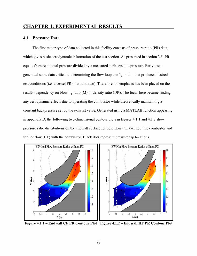
92

CHAPTER 4: EXPERIMENTAL RESULTS

4.1 Pressure Data

The first major type of data collected in this facility consists of pressure ratio (PR) data,

which gives basic aerodynamic information of the test section. As presented in section 3.5, PR

equals freestream total pressure divided by a measured surface/static pressure. Early tests

generated some data critical to determining the flow loop configuration that produced desired

test conditions (i.e. a vessel PR of around two). Therefore, no emphasis has been placed on the

results’ dependency on blowing ratio (M) or density ratio (DR). The focus here became finding

any aerodynamic effects due to operating the combustor while theoretically maintaining a

constant backpressure set by the exhaust valve. Generated using a MATLAB function appearing

in appendix D, the following two-dimensional contour plots in figures 4.1.1 and 4.1.2 show

pressure ratio distributions on the endwall surface for cold flow (CF) without the combustor and

for hot flow (HF) with the combustor. Black dots represent pressure tap locations.

Figure 4.1.1 – Endwall CF PR Contour Plot

Figure 4.1.2 – Endwall HF PR Contour Plot

93

Both plots indicate little variation in pressure ratio near the test section inlet at the left. Pressure

ratios of around one can be expected here since stagnation conditions usually occur toward the

vane’s leading edge (LE). When compared to distributions toward the pressure surface (PS),

greater PR along the vane suction surface (SS) indicates some flow adherence to this surface.

Flow through the passage toward the throat (the smallest area normal to the streamwise direction

along the passage) then accelerates thereby reducing static pressures. Hot flow introduces a slight

increase in static pressure toward the front of the vane’s suction surface (SS), which registers as

a small decrease in pressure ratio in this area. These two cases begin to noticeably vary from

around the throat region to the passage exhaust. Pressure ratios along the SS decrease more in the

hot flow case. As indicated by larger pressure ratios, low static pressures show some flow

separation occurring at the passage exhaust consistent with a sudden drastic increase in area.

Even the presence of a vortex structure at the exhaust can possibly be suggested. One can argue

that the hot exhaust gases simply increase overall flow pressure relative to a non-heated case. A

combination of the three effects should be considered when observing the hot flow’s pressure

ratio decrease of nearly 0.1 along the SS at the exhaust.

The next figure illustrates pressure ratio distribution along the vane surface at the

midspan plane (MP). Pressure ratios can be transformed into Mach numbers using simple

isentropic flow relations typically found in undergraduate thermodynamics textbooks. Mach

numbers reported in the figure legend have been computed at the leading edge, which has

pressure ratios of around one. Also, a hot flow case with film cooling can be seen in the plot.

While the reported blowing ratio of 5.57 falls outside the typical test conditions and may not be

an accurate calculation, this case does illustrate the fact that any film cooling air usually

increases static pressures along the surfaces. The film cooled case shows lower pressure ratios

across the entire vane surface than for the plain hot flow case. However, no film cooling holes

94

exist on the pressure vane as described in section 3.1.1. The logical conclusion for this

observable effect must be that air from the endwall film cooling holes impinges on the vane

surfaces to at least the midspan plane (MP).

Figure 4.1.3 – Vane Midspan Pressure Ratio Data

The other trends found in figure 4.1.3 can be seen in countless other presentations of

airfoil PR data. Low static pressures along the suction surface (SS) indicate flow acceleration,

which may be interpreted as higher PR along this surface denoted by negative s/c (arclength

divided by chord) locations. Once again, hot flow data suggests that the presence of combustion

gases reduces PR relative to the cold case. All cases have PR values converging to one at the

leading edge (s/c near 0), as expected since the stagnation point typically matches the vane LE.

Pressure recovery occurs along the pressure surface (PS) denoted by positive s/c locations.

Lower PR along this surface mean more lift force on the vane. The cold flow case has the lowest

PRs in the vicinity of s/c from 0.25 to 0.5. Hot flow decreases surface pressures possibly due to

some flow separation effects. Adding film cooling air seems to drive PR down to the cold flow

values in this small region. All three cases converge again slightly at around s/c of 0.6. Past this

95

point, PRS begin to match the trend of s/c around –1 on the SS. Such symmetry typically occurs

at the vane trailing edge (TE).

4.2 Normalized Metal Temperature (NMT) Data

Normalized metal temperatures (NMT) comprise the next type of data acquired in this lab.

Emphasis has been placed on blowing ratio (M), temperature ratio (TR), and/or density ratio

(DR) since effects of these parameters become more evident for heat transfer data. Each

presented data set tested only one TR for a day’s worth of data acquisition. Reasons for this

appear in section 4.3. The first data set of TR equal to 1.55 employed a test procedure that

experimented with maintaining the same TR at each M. This required minor adjustments to the

combustor exit temperature for each new M. At the present, only this mode of TR control exists,

but heaters mentioned in section 3.4 will allow more precise TR control in the future. Tested M

values range from about 0.5 to about 3.0 in increments of 0.25. Subsequent endwall (EW)

contour plots present the trends for key M cases.

These contours have diamond-shaped markers for film cooling hole locations and black

dots for heat flux gage/thermocouple positions. Figure 4.2.1 shows the majority of NMT values

staying within 0.1 to 0.2. This lowest M case of 0.5 expectedly has the smallest overall

performance since little film cooling air impinges on the EW surface. A small section of NMT

approaching 0.4 exists in the throat region near the PS, which may result from flow acceleration

toward the passage throat. Crossflow entering film cooling holes could be responsible for NMTs

of 0.1 near the test section inlet toward the LE. The next case of M equal to 1.0 sees a region of

higher NMT values starting to nucleate in figure 4.2.2. The region of highest NMT has migrated

from the throat toward the LE between the cases of M equal to 1.0 and 1.5. Increased coverage

from the first and second columns of film cooling holes causes NMT to approach 0.5 at M equal

96

to 1.5. Figure 4.2.3 also shows slightly lower NMT toward the PS at the test section inlet. Further

NMT improvement happens near the LE for the case of M equal to 2.0 in figure 4.2.4.

Figure 4.2.1 – EW NMT: M = 0.5, TR = 1.6

Figure 4.2.2 – EW NMT: M = 1.0, TR = 1.6

All of these low M cases do not exhibit any NMT improvement downstream of the throat.

Figure 4.2.3 – EW NMT: M = 1.5, TR = 1.6

Figure 4.2.4 – EW NMT: M = 2.0, TR = 1.6

A definite boundary has formed in figure 4.2.4 along the vane SS toward the LE as indicated by

NMT close to 0.55 in this area. This boundary forms a sharp NMT distribution near the inlet of

97

the passage when cross-passage flow migration that drives coolant away from the PS becomes

stronger at higher M. Marginal increases in NMT begin to manifest toward the TE at M equal to

2.0. Reduced performance in the region of highest NMT close to the test section inlet becomes

evident in figures 4.2.5 and 4.2.6. However, some benefits in NMT associated with more coolant

coverage occur along the SS toward the TE and along the PS toward the LE. Noticeable features

such as the “corner” near the PS at the test section inlet and the chordwise NMT spike close to

the vane SS remain in the two plots, but figure 4.2.6 shows these geometries becoming less

defined with even less NMT magnitude. Presumably, ideal performance exists somewhere

between M equal to 2.0 and 2.75 since some film separation possibly occurs at the higher M.

Figure 4.2.5 – EW NMT: M = 2.75, TR = 1.6

Figure 4.2.6 – EW NMT: M = 3.0, TR = 1.6

Vane line plots in figure 4.2.7 illustrate a spike in performance near the LE of the endwall

plane (EWP). Seemingly inconsistent trends exist in NMT distribution at the lowest M. For this

case of M equal to 0.5, the vane coolant supply plenum absorbs enough heat to give little benefit

in NMT especially near the LE for both endwall plane (EWP) and midspan plane (MP). NMT

performance in the EWP behaves expectedly as larger M values yield higher NMT.

98

Figure 4.2.7 – Vane NMT Line Plots for Nominal TR of 1.55

Performance drops accordingly with decreasing M. MP NMTs behave similarly at the LE and

along the PS, but two complete inversions occur in the NMT distribution along the SS. The first

of these two happens immediately upstream of the SS’s second column of film cooling holes,

which could indicate some flow blowing off of the SS at higher M. Another explanation could be

a passage vortex. Flow adheres again at an s/c around –0.55 where distributions invert once

more. Typical performance increases or decreases in roughly 0.015 increments for all M cases.

In an effort to determine what effect reducing run times would have, the next set of NMT

data applied the same experimental procedure a few days after collection of the previous data set

had taken place. A higher TR of 1.9 became the set point for this test. Some revision of the

LabVIEW program allowed reporting of coolant-to-freestream density ratios (DR). Evident in

the definition, density ratio depends on static pressures as well as temperatures. At low M, DR

equals TR, but coolant pressures rise with increasing M and, therefore, cause divergence between

99

DR and TR. Table 4.1 at the end of this section summarizes M, TR, and DR. In their titles, the

following endwall contour plots show DR spanning a range of 1.805 to 2.106 for the selected M

cases. Target M values began at around 0.75 and ended at around 3.0 in 0.25 increments. A

couple of contour plots have been omitted in order to better illustrate overall trends.

Quickly becoming a regular habit of low M, a small region of NMT close to 0.4

associated with undiluted flow acceleration begins to develop near the short column of film

cooling holes located in the passage’s throat area. NMT values around 0.2 surround this space in

figure 4.2.8. Darker blues toward the test section inlet indicate miniscule coolant coverage. The

region of NMT close to 0.4 grows in figure 4.2.9. This case of M close to 1.0 sees roughly the

same low NMT distribution near the test section inlet. Compared to a nominal TR of 1.55,

migration of the highest NMT values lags for M of 1.0 at TR of 1.9.

Figure 4.2.8 – EW NMT: M = 0.75, TR = 1.9

Figure 4.2.9 – EW NMT: M = 1.0, TR = 1.9

NMT distributions grow in figure 4.2.10 where coolant coverage improves downstream of the

second column of film cooling holes. This expanding area begins to engulf the entire passage

upstream of the throat and does not appear discriminatory to the SS. Slight PS to SS flow

100

migration possibly explains NMT values of 0.3 near the PS at the passage entrance. NMT

approaches 0.6 in the chordwise strip seen in figure 4.2.11. Even though this area’s location

appears somewhat stationary relative to the case of M equal to 1.5, NMT generally increases by

about 0.1 over the passage up to the throat. Once again, NMT improvements become negligible

at the TE for an M of 2.0.

Figure 4.2.10 – EW NMT: M = 1.5, TR = 1.9

Figure 4.2.11 – EW NMT: M = 2.0, TR = 1.9

Figure 4.2.12 shows small growth in and around the strip of highest NMT. Not much variation

exists between this case of M equal to 2.2 and the case of M equal to 2.4 pictured in figure

4.2.13. The latter case indicates some expansion of higher NMT values more toward the test

section inlet. These nearly invisible improvements could result from a lack of sufficient film

cooling air needed to incrementally lower metal temperatures at such a high TR.

101

Figure 4.2.12 – EW NMT: M = 2.2, TR = 1.9

Figure 4.2.13 – EW NMT: M = 2.4, TR = 1.9

Performance noticeably jumps at an M equal to 2.7. All of the familiar higher M features

presented in the previous case of TR equal to 1.55 appear in figure 4.2.14. The highest NMT

values occur at the front of the passage near the test section inlet.

Figure 4.2.14 – EW NMT: M = 2.7, TR = 1.9

Figure 4.2.15 – EW NMT: M = 2.9, TR = 1.9

However, sharpness in NMT distribution has lessened at the “corner” near the test section inlet

along the PS and at the third film cooling hole column. Hotter film layers in motion due to PS to

102

SS flow movement may explain this observation. This NMT distribution also seems to adhere to

the vane SS a little better over the entire surface. For the case of M equal to 2.9, NMT values at

the test section inlet undergo a small reduction, which might cause one to conclude that overall

performance decreases. Despite this reduction, NMT distributions finally exceed 0.5 across the

entire passage up to the throat. Figure 4.2.15 shows further NMT increases past the throat toward

the TE especially along the SS, which attracts flow. This indicates somewhat uniform coolant

coverage over the entire endwall and a decreased sensitivity to cross-passage flow migrations.


Predictable vane NMT trends appear in the line plots of figure 4.2.16. Just like figure

4.2.7, the lowest M of 0.7 produces the worst performance especially around the LE for both

planes. The increased TR causes NMT to be at its lowest closest to the LE on the EWP. An M of

1.3 bridges performance gap between the lowest two M cases and the rest of the cases. Except at

the inversion section of the MP, the case of M equal to 2.9 clearly possesses the best NMT

103

distribution. NMT performance falls with decreasing M in the EWP and in the MP from the LE

to the TE along the PS. The inversion beginning slightly downstream of the second column of

film cooling holes becomes rather jumbled. Although better than the case of M at 1.3, higher M

cases appear on the bottom due to flow separating from the SS. An s/c of around –0.55 sees a

restoration of order. Figure 4.2.16 most notably develops a peak in NMT near the LE in the MP.

This high TR case becomes the first to show mildly similar NMT distributions between EWP

and MP. In both planes, possible flow separations somewhat adversely affect NMTs downstream

of film cooling holes near the TE of the PS an SS.

Following an identical test procedure, the final NMT data set continues where the

previous set stopped. TR cases studied now include high (1.9) and intermediate (1.5) values, so

the next question became what effect a low TR has on NMT. Target M values started at 0.25

since the low TR allowed it. Eleven increments of 0.25 bring the maximum M tested to the

standard 3.0. At this constant TR of 1.1, reported DR values range between 1.092 and 1.371.

Once again, some endwall contour plots have been left out so that general trends become more

apparent.

An M equal to 0.25 had never been tested before mainly because the film cooling air

supply plenum absorbs significant amount of heat at the lower M. Higher TR cases pour even

more heat into the plenum, so those results potentially model no film cooling at all. Figure 4.2.17

shows NMT values of 0.2 and less. At the front of the test section, an area of NMT at around 0.1

seems to indicate some degree of sensitivity of the air exiting or potentially entering film cooling

holes in the proximity. This exact same region has the highest NMTs for high M cases seen at

other TRs. A form of symmetry obviously exists in this area. At M equal to 0.5, the typical

higher NMT zone driven by flow acceleration begins at the film cooling holes near the throat.

104

Depicted in figure 4.2.18, overall NMT seems to increase rapidly at all other places upstream of

the throat. Such an observation might indicate that NMT will rise very rapidly with M.

Figure 4.2.17 – EW NMT: M = 0.25, TR = 1.1

Figure 4.2.18 – EW NMT: M = 0.5, TR = 1.1

Figure 4.2.19 – EW NMT: M = 1.0, TR = 1.1

Figure 4.2.20 – EW NMT: M = 1.5, TR = 1.1

The NMT distribution in figure 4.2.19 confirms suspicions of rapid growth. Instead of a

migration of a region with higher NMT, an explosion of NMT centered on 0.4 fills the passage

up to the throat. Performance near the PS does seem to slightly lag behind. Further increases in

105

NMT occur in the upstream part of the passage in figure 4.2.20. This area now appears to be

rather uniform. Even the area immediately downstream of the throat starts to see some benefit.

Such distributions point to desirable uniform coolant coverage in the passage upstream of the

throat. This coverage most efficiently cools the surface for a lower TR.

Figure 4.2.21 – EW NMT: M = 2.0, TR = 1.1

Figure 4.2.22 – EW NMT: M = 2.5, TR = 1.1

Overall NMT improvements continue in figure 4.2.21, but the development of a higher NMT

region at the front of the test section shows a new mechanism by which this area appears. Unlike

previous TR cases, no migration occurred; this area sprang up somewhat spontaneously. Figure

4.2.22 illustrates a common evolution most likely driven by PS to SS flow migration, which may

be responsible for the higher NMT area’s sudden appearance in the case of M equal to 2.0. A

reduced TR possibly promotes better coolant-to-surface adhesion for lower M. Better adhered

coolant might be less susceptible to the PS to SS flow migration. Passage pressure gradients can

more easily drive thicker and less adhered coolant flow structures for M between 1.5 and 2.0.

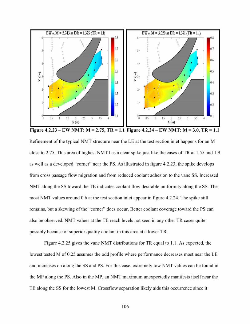
106

Figure 4.2.23 – EW NMT: M = 2.75, TR = 1.1

Figure 4.2.24 – EW NMT: M = 3.0, TR = 1.1

Refinement of the typical NMT structure near the LE at the test section inlet happens for an M

close to 2.75. This area of highest NMT has a clear spike just like the cases of TR at 1.55 and 1.9

as well as a developed “corner” near the PS. As illustrated in figure 4.2.23, the spike develops

from cross passage flow migration and from reduced coolant adhesion to the vane SS. Increased

NMT along the SS toward the TE indicates coolant flow desirable uniformity along the SS. The

most NMT values around 0.6 at the test section inlet appear in figure 4.2.24. The spike still

remains, but a skewing of the “corner” does occur. Better coolant coverage toward the PS can

also be observed. NMT values at the TE reach levels not seen in any other TR cases quite

possibly because of superior quality coolant in this area at a lower TR.

Figure 4.2.25 gives the vane NMT distributions for TR equal to 1.1. As expected, the

lowest tested M of 0.25 assumes the odd profile where performance decreases most near the LE

and increases on along the SS and PS. For this case, extremely low NMT values can be found in

the MP along the PS. Also in the MP, an NMT maximum unexpectedly manifests itself near the

TE along the SS for the lowest M. Crossflow separation likely aids this occurrence since it

107

requires little or no coolant coverage, or conduction effects heat up the plenum significantly. The

NMT spike near the LE of the EWP offers the highest values seen for all TR cases.


An M of 3.0 produces the best overall performance, which aptly falls off with decreasing M in

the EWP. Once again, this holds true along the PS in the MP. Performance in the MP along the

SS has a quasi-inversion shortly upstream of the second film cooling hole column. For s/c from

around –0.2 to –0.55, the cases of M equal to 0.5 and 0.8 as well as 0.25 give higher NMT values

than those of the highest M. An M of 3.0 does not appear to undergo any separation of film

cooling air, but the flow separation at lower M proves to be a dominant effect. All other cases

seem to jumble along the SS such that no noticeable benefit exists.

108

Figure 4.2.26 – EW Overall NMT for Different M at Nominal TR of 1.1, 1.6, and 1.9

All endwall NMT data from the previous three TR cases has been summarized in figure

4.2.26, which presents overall averaged NMT as a function of M. A general upward trend

confirms that NMT improves with increasing M. However, each TR case takes turns giving the

highest overall NMT values. At lower M, a TR of 1.1 gives coolant coverage that grows

uniformly up to an M of around 1.25. For M values between 1.25 and 2.5, strong PS to SS flow

migration causes the region of high NMT to develop quickly for the case of TR at 1.55. This

process happens faster for this case than it does for a TR of 1.9. Highly effective coolant

coverage near the test section inlet gives the highest TR an advantage for M above 2.5. At a TR

of 1.9 and an M around 3.0, more uniform coverage drops the highest NMT. Uniform coverage

for a TR at 1.1 causes a convergence in performance around an M of 3.0.

Vane overall NMT distributions pictured in figure 4.2.27 appear to take the exact same

shape between EWP and MP. A performance difference of about 0.05 exists between the two

planes. Both TR of 1.1 graphs increase virtually linearly with M and also give the best NMT

values for all M especially in the higher range.

109

Figure 4.2.27 – Vane Overall NMT for Different M at Nominal TR of 1.1, 1.5, and 1.8

As shown in the endwall contour plots, coolant coverage becomes most uniform at lower TR,

which might offer an explanation for why overall performance drops with increasing TR over the

vane surface. The graphs for TR equal to 1.8 seem to take an exponential form with NMT values

shooting up when vane plenum heat absorption ceases. This initial flow effect translates into a

knee shape for TR at 1.5. Overall NMT takes a nearly linear increase with M past about 0.75 at

this TR. The overall NMT plots of figures 4.2.26 and 4.2.27 confidently show the effects that M

and TR have on NMTs. This assurance stems from keeping each TR case isolated from each

other, which decouples any potential latent heat transfer effects associated with long test runs.

The following table summarizes the interrelationships between TR, M, and DR:

Table 4.1 – Interrelationship of TR, M, and DR DR / M

1.092 1.103 1.109 1.122 1.138 1.165 1.182 1.214 1.247 1.292 1.325 1.3711.1 0.255 0.506 0.745 1.023 1.260 1.563 1.716 1.997 2.227 2.528 2.743 3.020

--- --- --- --- --- --- --- --- --- --- --- --- 1.55 --- 0.505 0.741 0.988 1.260 1.511 1.731 2.010 --- 2.512 2.722 2.978--- --- 1.805 1.840 1.867 1.920 1.939 1.960 1.979 1.997 2.035 2.106

TR

1.9 --- --- 0.757 1.026 1.258 1.524 1.765 1.998 2.182 2.431 2.693 2.927

110

4.3 Heat Transfer Coefficient (HTC) Data

To continue the above discussion, the NMT data sets appearing in appendix F consisted

of three nominal TR cases all collected at the same time, which consumed a total time between

three and four hours. During one of those lengthy tests, the pressure vessel appreciably heats up

as a result of exhaust gases circulating inside the vessel after exiting the test section. Longer test

runs supply the pressure vessel with sufficient amounts of heat that then conducts through the

walls to the outside ambient air. This can significantly raise the overall temperature of the lab,

which indicates the magnitude of heat passing through the pressure vessel walls. However, the

amount of heat absorbed by the test section inside the pressure vessel becomes the real concern.

Adequate qualitative comparisons of heat transfer coefficients really cannot be made if the test

section releases heat left over from a previous TR test or from a lengthy test run. The

experimental procedure should focus on one TR at a time so that all heat fluxes start as close to

zero as possible for each TR case. The real information sought in these tests should be how heat

transfer to/from the test section surfaces according to some baseline conditions (i.e. all heat

fluxes zero). However, heat transfer coefficient (HTC) data must be corrected to account for non-

zero heat fluxes at ambient conditions with no flow. Such zero offsets should be obtained with

all valves closed. Presented HTC data has been corrected for such zero offsets

Because such a thing makes no physical sense, reported negative HTCs indicate that

negative heat fluxes have been measured by a particular heat flux gage. A negative measured

heat flux does not at all mean that the surface temperature exceeds the bulk crossflow

temperature. NMT values would also be negative if this were true. Instead, negative heat fluxes

result from hotter surfaces conducting heat to adjoining film layers. Typical film cooling

produces a cooler surface that absorbs heat from the film layer undergoing heating by the

crossflow. The results presented do offer some qualitative trends.

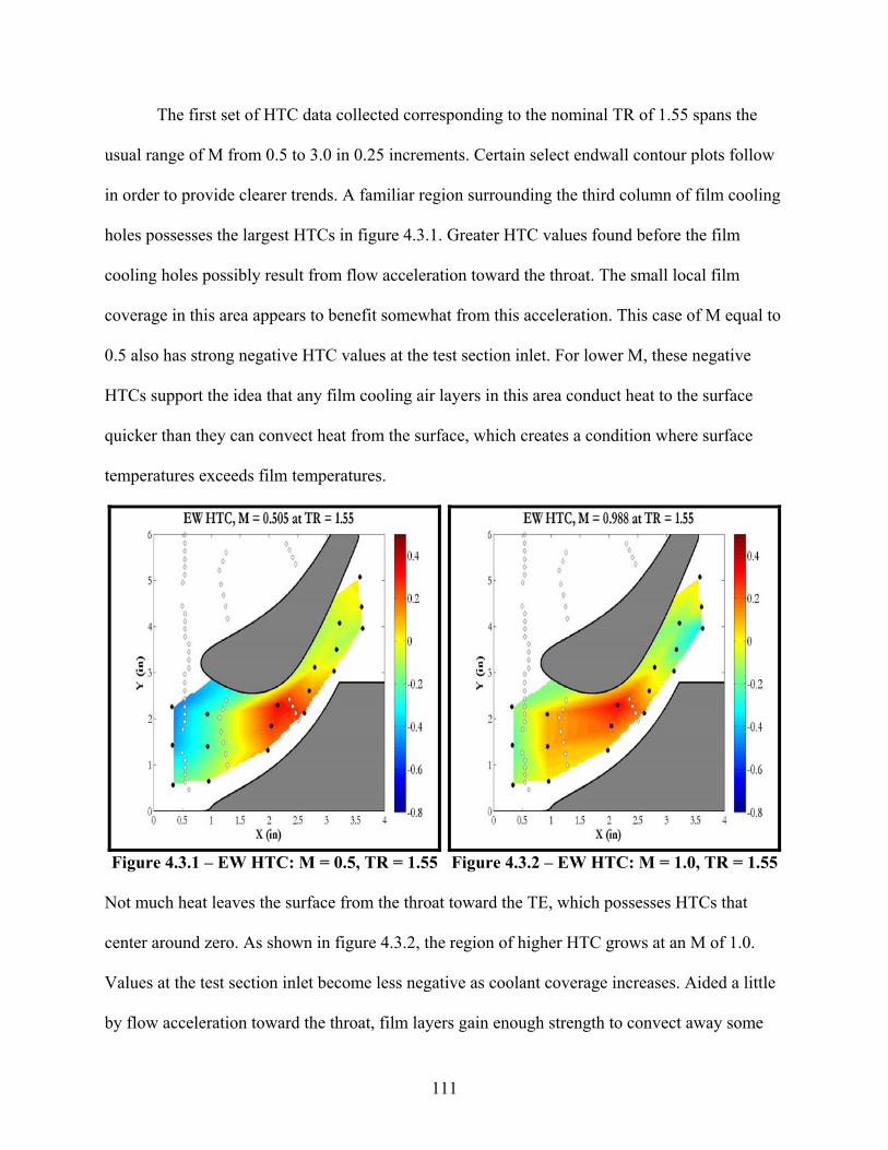
111

The first set of HTC data collected corresponding to the nominal TR of 1.55 spans the

usual range of M from 0.5 to 3.0 in 0.25 increments. Certain select endwall contour plots follow

in order to provide clearer trends. A familiar region surrounding the third column of film cooling

holes possesses the largest HTCs in figure 4.3.1. Greater HTC values found before the film

cooling holes possibly result from flow acceleration toward the throat. The small local film

coverage in this area appears to benefit somewhat from this acceleration. This case of M equal to

0.5 also has strong negative HTC values at the test section inlet. For lower M, these negative

HTCs support the idea that any film cooling air layers in this area conduct heat to the surface

quicker than they can convect heat from the surface, which creates a condition where surface

temperatures exceeds film temperatures.

Figure 4.3.1 – EW HTC: M = 0.5, TR = 1.55

Figure 4.3.2 – EW HTC: M = 1.0, TR = 1.55

Not much heat leaves the surface from the throat toward the TE, which possesses HTCs that

center around zero. As shown in figure 4.3.2, the region of higher HTC grows at an M of 1.0.

Values at the test section inlet become less negative as coolant coverage increases. Aided a little

by flow acceleration toward the throat, film layers gain enough strength to convect away some

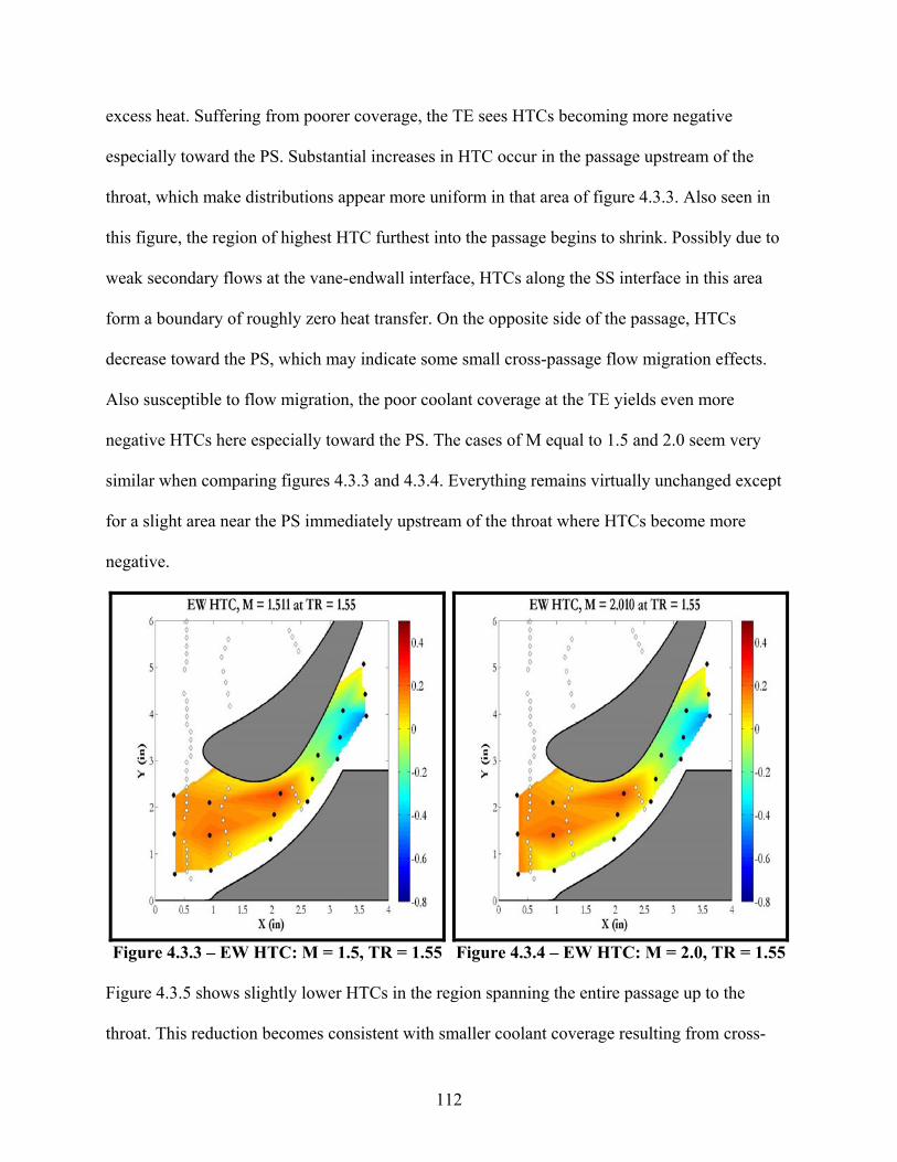
112

excess heat. Suffering from poorer coverage, the TE sees HTCs becoming more negative

especially toward the PS. Substantial increases in HTC occur in the passage upstream of the

throat, which make distributions appear more uniform in that area of figure 4.3.3. Also seen in

this figure, the region of highest HTC furthest into the passage begins to shrink. Possibly due to

weak secondary flows at the vane-endwall interface, HTCs along the SS interface in this area

form a boundary of roughly zero heat transfer. On the opposite side of the passage, HTCs

decrease toward the PS, which may indicate some small cross-passage flow migration effects.

Also susceptible to flow migration, the poor coolant coverage at the TE yields even more

negative HTCs here especially toward the PS. The cases of M equal to 1.5 and 2.0 seem very

similar when comparing figures 4.3.3 and 4.3.4. Everything remains virtually unchanged except

for a slight area near the PS immediately upstream of the throat where HTCs become more

negative.

Figure 4.3.3 – EW HTC: M = 1.5, TR = 1.55

Figure 4.3.4 – EW HTC: M = 2.0, TR = 1.55

Figure 4.3.5 shows slightly lower HTCs in the region spanning the entire passage up to the

throat. This reduction becomes consistent with smaller coolant coverage resulting from cross-

113

passage flow migration. HTC’s along the vane SS also undergo some reduction as that boundary

of zero HTC grows near the LE. An M equal to 2.7 offers increasing HTCs at the TE even

toward the PS. Despite any weak flow migrations, coolant coverage usually increases toward the

TE at higher M. Not many noticeable improvements can be seen in figure 4.3.6. As secondary

flow structures strengthen due to thicker coolant layers present for an M of 3.0, the boundary of

close to zero HTCs around the vane SS grows. Further reduction in HTC occurs near the test

section inlet toward the PS.

Figure 4.3.5 – EW HTC: M = 2.7, TR = 1.55

Figure 4.3.6 – EW HTC: M at 3.0, TR = 1.55

For the vane plots in figures 4.3.7 and 4.3.8, the lowest M of 0.5 exhibits a trend

reminiscent of the NMT plots in the previous section. Poor coolant coverage near the LE gives

way to unexpected benefits along the PS and SS for both EWP and MP. Flow acceleration

through the passage may help explain these benefits. For s/c from about –0.3 to about 0.4, EWP

HTCs improve with increasing M. Good quality coolant coverage comes from the film cooling

hole columns near the LE. This same trend happens in the MP over a smaller area centered about

the LE.

114

Figure 4.3.7 – Vane HTC Line Plots for Nominal TR of 1.5

Figure 4.3.8 – Expanded Vane HTC Line Plots for Nominal TR of 1.5

115

In the MP, HTCs for the highest M values drop after an s/c of 0.1 but then recover downstream

of the film cooling holes near the TE along the PS. A dip in HTC performance might indicate

some localized flow separation at higher M. MP HTC values show a familiar inversion at around

s/c equal to –0.1.Surface temperatures along the MP SS exceed film temperatures, which signify

poor quality coolant coverage. Two HTC distribution inversions can be seen along the SS on the

EWP graph. However, good HTC values occur in the EWP at s/c near –0.5, an area where

endwall contours reflect increases in HTC. For the higher M, coolant could be blowing off the

surface in this area, but some benefit can be observed from the third column of SS film cooling

holes. A lack of a LE HTC peak becomes most obvious in EWP graph, but this peak appears to

have migrated to the MP. This maximum’s presence at the MP could indicate uniform coolant

impingement from the film cooling holes along the vane surface.

Taken at a TR of 1.9, the next HTC data set followed the same experimental procedure

outlined for this TR in the NMT data section. Because of the high TR, M values only as low as

0.75 could be targeted. For the following endwall contour plots, a somewhat consistent trend

begins to develop at the test section inlet of figure 4.3.9. Strong negative HTCs result from the

poor coolant coverage effect being exacerbated by the higher TR. Coolant plenum temperature

sensitivity at lower M becomes more evident for a higher TR. Aided by flow acceleration toward

the throat in figure 4.3.9, a region of high HTC begins again around the throat but noticeably

shrinks toward the throat in figure 4.3.10. Along with this shrink comes a decrease in HTC

toward the test section inlet, which now has a sharp, corner-like distribution. The endwall

surfaces close to the first column of film cooling holes appear to be experiencing strong

conduction effects that reduce HTCs a little further downstream. A chordwise spike of HTCs

around zero begins to grow past the throat toward the TE.

116

Figure 4.3.9 – EW HTC: M = 0.75, TR = 1.9

Figure 4.3.10 – EW HTC: M = 1.0, TR = 1.9

A still visible corner with higher HTC exists at the test section inlet in figure 4.3.11. Better

coolant coverage significantly lowers surface temperatures everywhere in the passage into the

throat.

Figure 4.3.11 – EW HTC: M = 1.5, TR = 1.9

Figure 4.3.12 – EW HTC: M = 2.0, TR = 1.9

Flow acceleration and convergence carry increased coolant mass flow to the region upstream of

the throat. Lack of adequate coolant coverage causes HTCs to decrease toward the TE in figure

117

4.3.11 and in figure 4.3.12. The case of M equal to 2.0 sees complete dissipation of the

chordwise spike in the throat. HTC values at the test section inlet undergo further improvements

with increased coolant coverage.

Figure 4.3.13 – EW HTC: M = 2.2, TR = 1.9

Figure 4.3.14 – EW HTC: M = 2.4, TR = 1.9

Previously lagging areas at the test section inlet slowly approach HTC levels a little downstream

in figure 4.3.13. Overall, HTC values seem to thin out in the region dominated by larger HTCs.

The “corner” seen for previous M has been fully divided into two parts. One of these parts now

forms a small area of HTCs approaching zero along the vane SS near the LE. Figures 4.3.13 and

4.3.14 both show typical increasingly negative HTCs near the TE especially toward the PS. The

case of M equal to 2.4 sees further HTC benefits along the test section inlet fringes. However,

values begin to decrease along the PS here. Figure 4.3.15 shows the complete HTC evolution at

the test section inlet. Good quality film coverage finally occurs somewhat uniformly in this area.

HTC decreases may be seen along the PS toward the TE and toward the test section inlet. Lack

of coverage once again explains the former, and PS to SS flow migration offers some reason for

the other. The vane SS boundary becomes more well-defined at an M of 2.7.

118

Figure 4.3.15 – EW HTC: M = 2.7, TR = 1.9

Figure 4.3.16 – EW HTC: M = 2.9, TR = 1.9

At the highest M tested, that boundary of zero HTCs takes a more pronounced shape. Cross-

passage migration becomes a stronger effect along the PS toward the test section inlet in figure

4.3.16. Small increases in HTC finally reach downstream of the throat along the PS.

Along the vane surface, the cases of M equal to 0.75 and 1.0 both produce the HTC/NMT

profile characteristic of lower M. Figure 4.3.17 illustrates an extreme nadir near the LE in the

EWP. Better behavior of the EWP cases can be seen in figure 4.3.18, which shows HTCs

growing with increasing M from an s/c of about –0.3 to an s/c of about 0.4. The MP once again

has a small area of expected behavior centered on the LE. Some slight inversion of the highest M

cases along the PS results in a recovery toward the TE in figure 4.3.18. The typical MP inversion

occurs immediately upstream of the second column of film cooling holes. Both the EWP and MP

graphs appear quite similar to those of a TR at 1.5 and at 1.8. Once again, the LE peak in MP

replaces that seen in the EWP for the NMT data.

119



120

In the final set of HTC data, a TR of 1.1 allowed for target M values to begin at 0.25 and

end with 3.0. The experimental procedure for this TR stayed the same as the previous TR case.

Figure 4.3.19 clearly illustrates what effect TR has on HTC. Less negative values appear at the

test section inlet for this lowest TR and M. A smaller crossflow-to-coolant plenum temperature

gradient decreases surface temperatures relative to higher TR counterparts. For this lowest M,

only the flow acceleration toward the throat drives the region of highest HTC. Near the TE, HTC

values stay around zero over the entire passage. Slight overall reductions occur in this same area

in figure 4.3.20. Increasing HTCs upstream of the throat begin to create a familiar sharp, corner-

like geometry of slightly lower HTC at the test section inlet. All areas in this passage inlet

experience some benefits due to more film cooling air.

Figure 4.3.19 – EW HTC: M = 0.25, TR = 1.1

Figure 4.3.20 – EW HTC: M = 0.5, TR = 1.1

The case of M equal to 1.0 sees higher HTC values filling the passage inlet upstream of the

throat. Areas in this region along the PS seem to experience slower improvements. However,

figure 4.3.21 shows HTC decreases along the PS near the TE. Some cross-passage flow

migration of marginal amounts of coolant air might help explain this.

121

Figure 4.3.21 – EW HTC: M = 1.0, TR = 1.1

Figure 4.3.22 – EW HTC: M = 1.5, TR = 1.1

The area downstream of the throat remains virtually identical in figure 4.3.22, which signifies

little benefit of increased M here. Toward the test section inlet, increases in HTC values make

this region a bit more uniform. Larger amounts of coolant cause the boundary of zero HTC to

develop along the SS near the LE for an M of 1.5.

Figure 4.3.23 – EW HTC: M = 2.0, TR = 1.1

Figure 4.3.24 – EW HTC: M = 2.5, TR = 1.1

122

Negligible improvements in HTC occur at the test section/passage inlet for figures 4.3.23 and

4.3.24. At these M values equal to 2.0 and 2.5, more film cooling air possibly becomes inertially

limited in its ability to convect heat away from the surface. The two figures look quite similar

except for the minute increase of HTC along the PS near the TE, which begins to see some

benefit from slightly increased coolant coverage that resists cross-passage migration. A small

growth of the zero HTC boundary can be observed for the higher M.

Figure 4.3.25 – EW HTC: M = 2.7, TR = 1.1

Figure 4.3.26 – EW HTC: M = 3.0, TR = 1.1

Reduced HTCs at the test section inlet appear in figure 4.3.25. This area may be

experiencing some separation of film cooling air or reduced benefits associated with a lower TR.

Along the PS, cross-passage flow migration possibly decrease HTCs in that region. Toward the

TE, coolant coverage further increases due to greater amounts of film cooling air at the higher M.

All trends present in the case of M at 2.7 intensify for the final case of M equal to 3.0. HTCs

noticeably decrease at the passage inlet upstream of the throat, which possibly experiences

slightly more coolant separation at the highest M. Both added coolant and growing secondary

123

flow structures augment the size of the zero HTC boundary along the vane SS near the LE. The

TE HTC distribution appears unchanged by the increase in coolant.

Vane plots in figure 4.3.27 expectedly show the typical HTC distribution in the EWP for

the low M of 0.25. This same case surprisingly has decent performance near the LE in the MP.

HTC distributions become more familiar along the MP PS and SS. The expanded plots of figure

4.3.28 illustrate HTCs that improve with increasing M for the majority of the EWP. The highest

HTC values occur near the LE in the EWP but more along the PS possibly because of better

adhered coolant layers from the LE holes. Most likely due to some flow separation, some slight

inversion and convergence occurs in the EWP immediately upstream of the last SS film cooling

hole column.


Coolant rejoins the surface at an s/c around –0.5. HTC values in the MP undergo three inversions

as seen in figure 4.3.28. Complete inversion along the SS begins immediately upstream of the

124

second film cooling hole column. Flow separation effects first indicated in the EWP intensify in

the MP where an M of 0.5 gives some of the best coverage along the SS. The second MP HTC

inversion happens right next to the LE. In this area, a lower TR provides a smaller range of

surface and film temperatures that result in higher HTC. Recovery shortly upstream of the last

PS column of film cooling holes indicates some benefit from increased coolant through these

holes.


The somewhat jagged line plots of figure 4.3.29 illustrate overall averaged endwall

HTCs. Even though only negative values appear, the plots indicate that the lowest TR of 1.1

performs the best at lower M from 0.25 to 0.75. Lower crossflow-to-coolant temperature

gradients for this lowest TR increase HTCs through a strong coupling with flow acceleration

toward the throat. From M around 1.0 to M around 1.5, the case of TR at 1.6 has HTC values

that match those of the lowest TR case. Performance converges at around an M of 1.5 at which

125

some form of HTC balance exists for all three cases. The highest and lowest TR cases give better

HTC than the middle case, which drops off for larger M. For the case of TR equal to 1.6, strong

cross-passage flow migration effects appear along the PS at the test section inlet and near the TE.

These effects promote slightly higher HTC with an increase in TR. PS to SS flow migrations at

the test section inlet and at the exhaust weaken at the lowest TR most likely because of better

adhered coolant layers. Past an M of 2.5, overall HTCs drop for TR of 1.9. Cross-passage

migration strengthens as more flow blows off the surface at higher M.

Figure 4.3.29 – EW Overall HTC for Different M at Nominal TR of 1.1, 1.6, and 1.9

In the vane EWP, HTC performance seems largely unaffected by TR. After the odd HTC

distributions for lowest M, a general upward trend with M becomes noticeable in figure 4.3.30.

Growth of the boundary of zero HTC on the endwall surface loses ground to improvements with

increasing M everywhere else along the vane PS and SS. The case of TR equal to 1.5 gives a tiny

advantage over the entire range of M from 0.75 onward. Parabolic shaped curves replace the

general upward trends for the MP line plots. Each TR case has low HTCs at low M but then

shoots up to some maximum at a higher M. For the MP, overall HTC appears best at a low TR

and a lower M of around 1.0. After an M of around 1.5, a TR of 1.5 offers the best HTC values

126

relative to the other two cases. Performance for all three cases worsens with increasing M

possibly due to coolant flow separation along the SS in the vane MP.

Figure 4.3.30 – Vane Overall HTC for Different M at Nominal TR of 1.1, 1.5, and 1.8

127

CHAPTER 5: CONCLUSIONS AND RECOMMENDATIONS

Pressure data collected for both hot and cold flow without film cooling show rising

pressure ratios along the endwall near the passage throat. These increasing pressure ratios signify

flow acceleration through the throat. The highest pressure ratios occur toward the TE, which

indicates some flow separation in this area. Heated reacting flow raises surface pressures as

evident in the lower pressure ratios from the throat inlet to the exhaust in the hot flow case.

Pressure ratio distributions along the vane surface show flow separation along the SS and

pressure recovery along the PS. Cases with hot flow have slightly lower pressure ratios over the

majority of the vane surface. The presence of film cooling air from the endwall drives pressure

ratios along the vane surfaces even lower than plain hot flow alone, which results from increased

static pressure accompanying film cooling impingement on the vane surface.

All NMT data illustrates rises in performance with increasing M. At each separate case of

TR targeted for 1.1, 1.5, and 1.9, NMT performance decreases drastically toward the lower M

values. Two processes appear to drive this. First, smaller amounts of film cooling air actually

conduct heat into coolant plenums due to reduced heat capacity. At M around 0.25 to 0.75,

coolant coverage becomes hotter than the endwall or vane surfaces in the initial impingement

onto these surfaces, which impedes the coolant’s ability of convecting heat as coolant layers

grow on the surface. This effect appears most visibly near the vane LE and near the test section

inlet on the endwall. Both of these areas coincidentally have the most film cooling holes. On the

endwall, regions of high NMT appear to migrate from the passage throat to the test section inlet

as M increases for the two higher TRs of 1.55 and 1.9. Similar well-defined geometries of high

NMT seem to pop up at higher M for the case of TR equal to 1.1. On the endwall, overall NMT

plots show net increase of 0.25 over the entire tested span of M with each TR case giving the

best performance in specific M intervals. These divisions occur due to increases in coolant

128

coverage uniformity. A definite peak in NMT performance along the vane surface occurs near

the LE in the EWP where film cooling air from both the vane and the endwall impinges on the

surface. For all three TR cases, EWP NMT distributions improve by about 0.025 with increasing

M over the entire tested range. Smaller NMT values around the vane TE indicate thinning or

separation of film cooling layers. The MP exhibits no dominant peak around the LE. In general,

improvements to MP NMT have smaller magnitudes than their EWP counterparts. A curious

performance inversion occurs in the MP along the beginning of the SS. Higher M yields lower

NMT at this juncture, which might indicate flow separation. The inversion reverses itself for all

three TR cases at around an s/c of –0.55. Overall vane NMT line plots clearly illustrate

performance dropping off with increasing TR. The lowest TR of 1.1 gave net NMT increases of

about 0.12 and 0.07 on the EWP and MP, respectively. Each TR case graph takes on different

shapes that seem to evolve from a near exponential at a TR of 1.8 to the line for the case of TR at

1.1.

Even though HTC data reports negative values, significant consistent trends can still be

extracted. Negative HTCs indicate negative measured heat fluxes, q”, which stem from test

section surfaces losing heat to film cooling air layers in the steady state. Positive local HTCs

assuredly exist along the interface between the metal surfaces and the film layers. HTCs

presented in the preceding chapter have been defined for heat transfer between the metal surfaces

and the bulk crossflow. Along the endwall surfaces, all three targeted TRs tested show most

negative HTC values near the test section inlet at low M. This observation becomes consistent

with the explanation for small NMT values in this same area at low M. A TR of 1.9 produces the

most negative HTCs in the area near the test section inlet since required elevated combustor

temperatures heat up that area significantly. Also in these cases of low M, high HTCs toward the

throat area indicate simple flow acceleration of the crossflow along the endwall. As M rises in all

129

TR cases, HTCs increase in the passage upstream of the throat. Increased coolant coverage

produces more uniform HTC distributions in this region. A TR of 1.1 develops these more

uniform HTC’s the quickest and maintains them over a large range of M. HTCs downstream of

the throat become slightly more negative with increasing M due to a smaller amount of film

cooling holes as well as growing cross-passage flow migrations of thicker film layers. At high

M, all TR cases exhibit cross-passage flow migration near the PS at the test section inlet. HTC

data near the LE on the vane surface reflect endwall trends at low M. Increasing M results in a

HTC peak in the MP. More observable changes in HTC occur in the MP than for the EWP.

However, increasing M does generally increase HTCs. The vane SS provides an exception to this

in both vane planes for all TR cases. Thinning coolant layers along the SS may be the culprit for

diminishing benefits with increasing M. Vane overall HTC plots expectedly show little variation

between TR cases in the EWP. Distributions in the MP indicate a specific M for each TR where

HTC reaches a maximum. In the MP, the largest overall HTC of about 0.02 R2BTU ft s o occurs

at a TR of 1.1 and an M of around 1.0.

The test procedure used to obtain the above results consisted of maintaining certain target

TR values. Amongst other observations, DR intuitively rises with M. The pressure ratio between

coolant and crossflow becomes larger at high M. DR depends directly on the coolant-to-

crossflow pressure ratio and expectedly increases. Further experiments could have some means

to better control TR and possibly even DR. More pertinent pressure ratio data should give an

increased understanding of how M and DR vary over test section surfaces. For future work,

negative measured heat fluxes must be studied in greater detail. No instrumentation exists to

measure film temperatures very close to the test section surfaces, so an extremely accurate

representation of HTC cannot be provided at this point. A complete set of infrared (IR)

130

measurements could offer more insight. The current HTC definition should most certainly be

reconsidered and expanded to give some account for film temperatures.

131

REFERENCES

[1] Sieverding, C.H., W. Van Hove, and E. Boletis. “Experimental Study of the Three-Dimensional Flow Field in an Annular Turbine Nozzle Guidevane.” ASME Journal of Engineering for Gas Turbines and Power 106 (1984): 437-444.

[2] Boletis, E. “Effects of Tip Endwall Contouring on the Three-Dimensional Flow Field in an

Annular Turbine Nozzle Guide Vane: Part I – Experimental Investigation.” ASME Journal of Engineering for Gas Turbines and Power 107 (1985): 983-990.

[3] Moustapha, S.H., and R.G. Williamson. “Effect of Two Endwall Contours on the

Performance of an Annular Nozzle Cascade.” AIAA Paper No. 85-1218 (1985). [4] Kang, M.B., and K.A. Thole. “Flowfield Measurements in the Endwall Region of a Stator

Vane.” ASME Journal of Turbomachinery 122 (1999): 458-466. [5] Burd, S.W., and T.W. Simon. “Flow Measurement in a Nozzle Guide Vane Passage with a

Low Aspect Ratio and Endwall Contouring.” ASME Journal of Turbomachinery 122 (2000): 659-666.

[6] Kopper, F.C., R. Milano, and M. Vanco. “An Experimental Invetigation of Endwall

Profiling in a Turbine Vane Cascade.” AIAA Paper No. 80-1089 (1980). [7] Duden, A., I. Raab, and L. Fottner. “Controlling the Secondary Flow in a Turbine Cascade

by Three-Dimensional Airfoil Design and Endwall Contouring.” ASME Journal of Turbomachinery 121 (1999): 191-199.

[8] Dossena, V., A. Perdichizzi, and M. Savini. “The Influence of Endwall Contouring on the

Performance of a Turbine Nozzle Guide.” ASME Journal of Turbomachinery 121 (1999): 200-208.

[9] Hartland, J.C., D.G. Gregory-Smith, N.W. Harvey, and M.G. Rose. “Nonaxisymmetric

Turbine Endwall Design: Part II – Experimental Validation.” ASME Journal of Turbomachinery 122 (2000): 286-293.

[10] Zess, G.A., and K.A. Thole. “Computational Design and Experimental Evaluation of Using

a Leading Edge Fillet on a Gas Turbine Vane.” IGTI Conference Paper No. 2001-GT0404, New Orleans 2001.

[11] North American Manufacturing Company: “Zephyr™ Integral Blower, Gas Burners.” N.A.

Manufacturing Company Bulletin 4988 (2006). [12] Zander, Inc.: "Series KN: KN Heatless Desiccant Compressed Air Dryers." Zander, Inc

(2004). [13] Scanivalve Corp.: “Digital Sensor Array: DSA 3000 Series Modules & DSA 3200 Series

Modules Instruction and Service Manual.” Scanivalve Corporation (2001).

132

[14] National Instruments: “FieldPoint™ Operating Instructions: FP-TC-120 and cFP-TC-120

(8-Channel Thermocouple Input Modules).” National Instruments Corporation (2002). [15] National Instruments: “FieldPoint™ Operating Instructions: FP-AI-112 and cFP-AI-112

(16-Channel, 16-Bit Analog Input Modules).” National Instruments Corporation (2004). [16] Medtherm Corporation: “Description, Method, and Interpretation of Calibration of Heat

Flux Transducers P/N 4H-50-36-36-20753.” Correspondence sent to General Electric Power Systems Company, P.O. No. 41002130 & Job No. 20-13663 (2004).

[17] National Instruments: “FieldPoint™ Operating Instructions: cFP-CB-1 and cFP-CB-3

(Compact FieldPoint™ Connector Blocks).” National Instruments Corporation (2003). [18] Sierra Instruments: “640S Series Steel-Mass™: Smart Insertion, Thermal Gas, Mass Flow

Meter.” Sierra Instruments Inc. (2004). [19] Sierra Instruments: <http://www.sierrainstruments.com/products/640.html> (2009). [20] National Instruments: “FieldPoint™ Operating Instructions: FP-AIO-600 and cFP-AIO-

600 (4-Channel Analog Input & 4-Channel Analog Output, 12-Bit Module).” National Instruments Corporation (2006).

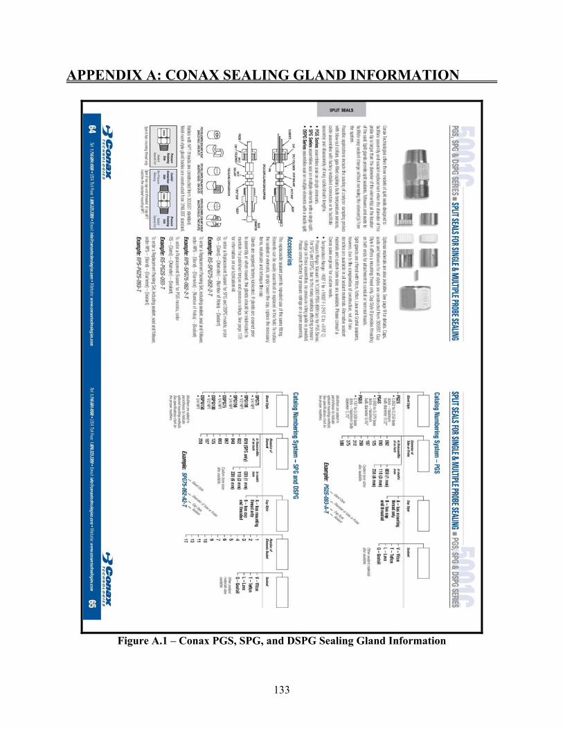
133

APPENDIX A: CONAX SEALING GLAND INFORMATION

Figure A.1 – Conax PGS, SPG, and DSPG Sealing Gland Information

134

APPENDIX B: STAHL COMBUSTOR DRAWINGS

Figure B.1 – Stahl Combustor Drawing 33763

135


136


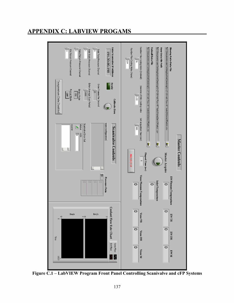
137

APPENDIX C: LABVIEW PROGAMS

Figure C.1 – LabVIEW Program Front Panel Controlling Scanivalve and cFP Systems

138

Figure C. 2 – State Machine Structure of LabVIEW Program with Main States Shown

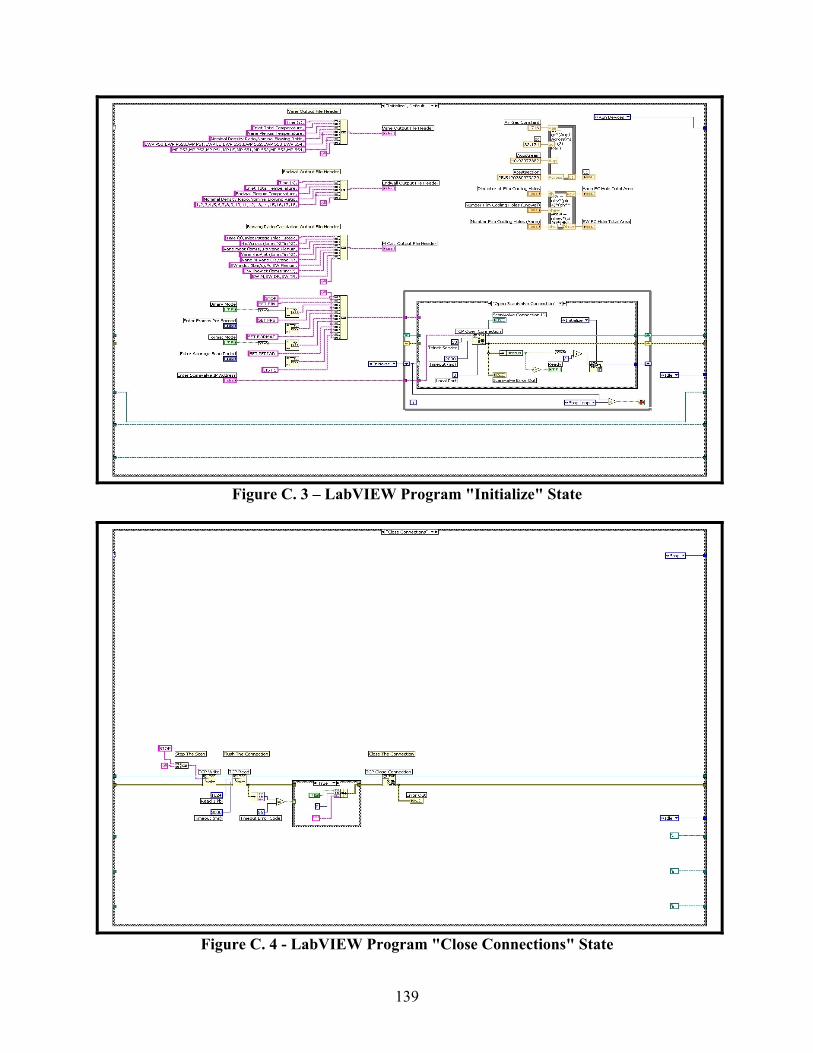
139

Figure C. 3 – LabVIEW Program "Initialize" State

Figure C. 4 - LabVIEW Program "Close Connections" State

140

APPENDIX D: HF GAGE CALIBRATION CURVE

Figure D.1 – Typical Medtherm HF Gage Responsivity Curve

141

APPENDIX E: MATLAB PROGRAMS

This MATLAB program acts as a separate function called from other programs in order

to produce contour plots.

function [] = EWContourPlot(z,contourplottitle,contourlimits,filename) clear plots FCHoles = xlsread('TestSectionInfo.xls', 'EWFCLocations', 'B5:E56'); InstLocs = xlsread('TestSectionInfo.xls', 'TapLocations', 'B3:D20'); FlatVaneProf = xlsread('TestSectionInfo.xls', 'FlatVaneProfile', 'A3:C495'); FlatEWProf = xlsread('TestSectionInfo.xls', 'FlatEWProfile', 'A3:C215'); [X,Y] = meshgrid(0:0.05:4,0:0.05:6); Z = griddata(InstLocs(:,1),InstLocs(:,3),z,X,Y,'linear'); fig = figure('Color','w','PaperUnits','inches','PaperSize',[4 5.5]); axes('Box','on','Color',[0.82 0.82 0.82],'XLim',[0 4],'YLim',[0 6],'FontName','Garamond','FontSize',12); title(contourplottitle,'FontName','Garamond','FontSize',16,'FontWeight','bold'); xlabel('X (in)','FontName','Garamond','FontSize',14,'FontWeight','bold'); ylabel('Y (in)','FontName','Garamond','FontSize',14,'FontWeight','bold'); hold on [C,c1] = contourf(X,Y,Z,200); set(c1,'LevelList',contourlimits,'LineStyle','none'); colorbar('FontName','Garamond','FontSize',14); caxis([min(contourlimits) max(contourlimits)]); s1 = scatter(FCHoles(:,1),FCHoles(:,4)); set(s1,'Marker','d','MarkerEdgeColor','k','MarkerFaceColor','w'); s2 = scatter(InstLocs(:,1),InstLocs(:,3)); set(s2,'Marker','o','MarkerEdgeColor','k','MarkerFaceColor','k'); f1 = fill(FlatVaneProf(:,1),FlatVaneProf(:,3),[0.5 0.5 0.5],FlatEWProf(:,1),FlatEWProf(:,3),[0.5 0.5 0.5]); set(f1,'EdgeColor','k','LineWidth',2); saveas(fig,filename); close

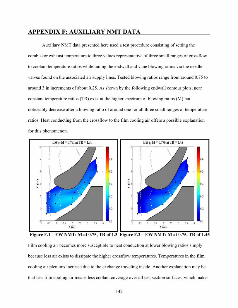
142

APPENDIX F: AUXILIARY NMT DATA

Auxiliary NMT data presented here used a test procedure consisting of setting the

combustor exhaust temperature to three values representative of three small ranges of crossflow

to coolant temperature ratios while tuning the endwall and vane blowing ratios via the needle

valves found on the associated air supply lines. Tested blowing ratios range from around 0.75 to

around 3 in increments of about 0.25. As shown by the following endwall contour plots, near

constant temperature ratios (TR) exist at the higher spectrum of blowing ratios (M) but

noticeably decrease after a blowing ratio of around one for all three small ranges of temperature

ratios. Heat conducting from the crossflow to the film cooling air offers a possible explanation

for this phenomenon.

Figure F.1 – EW NMT: M at 0.75, TR of 1.3


Film cooling air becomes more susceptible to heat conduction at lower blowing ratios simply

because less air exists to dissipate the higher crossflow temperatures. Temperatures in the film

cooling air plenums increase due to the exchange traveling inside. Another explanation may be

that less film cooling air means less coolant coverage over all test section surfaces, which makes

143

these surfaces conduct heat into the plenums more easily. Zero can be considered the theoretical

lower limit for NMT while an NMT closer to one shows better film cooling performance.

Figures F.1 and F.2 show NMT values staying in the 0.1 to 0.3 range for the cases of M at about

0.75.The highest NMT appears to exist shortly upstream of the throat region, which might be

experiencing some coolant coverage from the second “column” of film cooling holes. Also,

NMT seems to improve as TR decreases as observed by the obvious color change from dark blue

to light blue toward the leading edge. The contour plots in figures F.3 to F.5 reflect the same

trend for M around 1.0. A large region of NMT at about 0.35 can be found toward the LE

concentrated in the middle of the passage in the lowest TR case.



This probably occurs from increased coolant coverage from the first two “columns” of film

cooling holes. A particularly interesting similarity exists between M at 0.75 for the lowest TR

and M at 1.0 for the other two TRs. This perfectly illustrates the functional interdependence of M

on TR that physically manifests itself in the changing heat capacity of the film cooling jet. Little

NMT variation occurs between TR of 1.49 and TR of 1.63 at M around 1.0. Some contour plots

144

of in between M cases have been omitted in order to present more general trends. Considerable

increases in NMT can be seen at M around 1.5. Nearly negligible increases in NMT still exist

near the TE, but a strong region of higher NMT begins to develop downstream of the first

column of film cooling holes. Illustrated in figure F.6, this area appears to lie closer to the SS.

Figure F.7 somewhat mirrors figure F.3 with a depiction of this area’s migration toward the LE.





145

Figure F.8 shows reduced NMT values at M equal to 1.5, but this case’s highest values appear

concentrated more to the PS. The next case of M close to 2.0 indicates a further migration of the

higher NMT area toward the LE. As presented in figure F.9, better coolant coverage comes from

the first column of film cooling holes. Higher M expectedly increases effectiveness across the

board. However, the smallest NMT values remain near the TE, which most probably results from

an absence of film cooling holes in this area. An interesting trend begins to develop between the

cases of TR equal to 1.35 and TR equal to 1.56. Evidenced by figures F.9 and F.10, NMT

distributions appear to be near identical downstream of the second column of film cooling holes.

Figure F.11 illustrates performance lagging at higher TR, but the familiar migration process

noticeably starts around M equal to 2.0 for this TR.

Figure F.9 – EW NMT: M at 2.0,TR of 1.35


At M close to 2.5, the original trend of performance decreasing with increasing TR begins to

reverse. NMT values of around 0.6 and above can be seen in figure F.13 near the LE for the case

of TR equal to 1.57. The same region in figure F.12 has obviously smaller values.

146



Just like the previous M case, similarity after the second film cooling hole column exists in

figures F.12 and F.13. Once can also observe the development of a sharp divide in NMT

distribution around the first column of film cooling holes near the PS. This indicates a migration

of film cooling air from the PS toward the SS as it enters the passage.



147

The observed evolution of high NMT values toward the LE could come as a result of this flow

migration. At a TR of 1.83, NMT values finally reach a level of 0.5 as seen in figure F.14. This

case reflects the trend of figure F.10 except toward the TE where performance increases in the

case of M close to 2.5. Although having the best overall performance near the TE, figure F.15

shows noticeably decreased NMT values downstream of the second film cooling hole column

when compared to figure F.13. This establishes TR of 1.57 as giving the best performance at

higher blowing ratios.



The best coolant coverage can be seen in figure F.16 where NMT values reach around 0.7.

However, performance stays nearly the same at the TE for M between 2.5 and 3.0 at a TR of

1.57. All of the above trends become apparent in figure F.17, which summarizes averaged NMT

values as a function of M for the three nominal TR cases studied. Nominal TR has been

computed as the average of all the TR values associated with each case. The general upward

trend expectedly appears with NMT increasing from 0.1 to 0.4. An intersection occurs between

the nominal TRs of 1.3 and 1.5 at an M slightly greater than two. Performance seems to level off

148

with increasing M, but a definite maximum can be seen at M around 2.75 for a nominal TR of

1.5. The case of nominal TR equal to 1.8 gives the worst overall performance even though at

around an M of 2.5 it begins a trend that presumably would exceed the other two cases. For this

TR case, maintaining stable M from 3.0 to 2.75 proved somewhat unusually difficult, so data

presented in this range may not be exactly trustworthy.

Figure F.17 – EW Overall NMT for Different M at Nominal TR of 1.3, 1.5, and 1.8

The next few plots present NMT data generated for the vane at nominal TR of 1.3, 1.4,

and 1.6. Again, actual TR varies between M cases; a nominal TR averages of this distribution.

Vertical dashed lines on the figures represent film cooling hole “columns” drilled over the entire

span of the heat transfer vane depicted in section 3.1. Also discussed in that section, the

instrumentation found on the heat transfer vane has been located at two “planes” appropriately

deemed “EWP” and “MP” for endwall plane and midspan plane, respectively. Vane plot legends

indicate the target M values.

149

Prominently featured in figure F.18, wide NMT variation exists between EWP and MP

for all M cases. Further comparison focuses this difference mainly to the LE (s/c of 0), which has

a definite peak on the EWP. This region of NMT at around 0.9 has a couple of possible

explanations. Film cooling air could be impinging on the vane surface from the endwall film

cooling holes as evidenced by the vane pressure ratio data in the previous section. The EWP sees

more film cooling air simply because it lies right next to the endwall. Localized uneven film

cooling air flow distribution might offer another reason. More air flows at the EWP, which lies

closer to the film cooling air supply plenum. However, this unlikely possibility overtly

contradicts assumptions made when developing methods for calculating M.

Figure F.18 – Vane NMT Line Plots for Nominal TR of 1.3

Also, the MP has larger NMT off of the LE along the SS and PS (negative and positive s/c). In

this area, the roughly 0.05 increase gives an inconsistency to the uneven flow idea since NMT

values exist the same neighborhood of 0.4 to 0.6. The next observable trait in this figure

150

expectedly shows the lowest NMT distribution for the lowest M, but the highest M of 3.1 has a

performance right next to the lowest M. This holds true for the entire MP and for the majority of

the EWP, which has been expanded in figure F.19. At this M, flow most likely blows off the

vane surface. The rest of the MP cases undergo somewhat of an inversion at around the LE.

Higher M cases have lower performance on the SS then show improvements at the LE before

converging with other M cases along the PS. Combined with the EWP NMT spike, this effect

indicates some benefit from the film cooling hole arrangement near the LE. Comparatively, film

cooling holes near the TE on the PS show smaller improvements even though these holes point

toward the TE. Similarly, one would expect the last film cooling hole column on the SS to

increase NMT downstream toward the TE. Coolant flow most likely has not been distributed

along the PS and SS by the same mechanism that apparently drives coolant flow over the LE

surface from film cooling holes parallel to the span direction.

Figure F.19 – Expanded Vane NMT Line Plots for Nominal TR of 1.3

151

Lower NMT values become the first noticeable feature of figure F.20 when compared to

figure F.18. Still present in this case of nominal TR equal to 1.4, the EWP spike has a slightly

smaller in magnitude. A feature also illustrated in this figure becomes characteristic of tests at

higher TR. M values close to 0.75 provide the vane surface with very small coverage layers that

conduct heat more than dissipate it. Extremely low NMT values at the LE point to appreciable

heat conducting to the vane supply plenum through the film cooling air. Also, some hot

crossflow air quite possibly flows into the plenum through the film cooling holes since jet

pressure falls with decreasing M. Slightly higher that those for M equal to 0.75, NMT values for

M close to 2.8 and 2.7 mirror the distribution of M equal to 1.0. A clear divide exists in figure

F.21 with the middle M cases getting better performance than the highest and lowest M cases.

These middle M cases have nearly the same NMT distributions. However, an M between 1.6 and

1.8 performs the best of the middle cases even though not much variance exists in the MP curve.

Figure F.20 – Vane NMT Line Plots for Nominal TR of 1.4

152

Figure F.21 – Expanded Vane NMT Line Plots for Nominal TR of 1.4

The final nominal TR case of 1.6 maintains many of the general trends of the other two

cases including very low NMT values at lower M. Figure F.22 presents more intuitive data than

the previous nominal TR case. In general, higher M values yield better performance with an M of

3.9 giving the best at the LE of the EWP. Previously stated, this M case might not have reliably

“steady state” data even though it follows the same trends. The M equal to 1.0 case takes a rather

odd form. Performance along the SS and PS where less film cooling holes exist exceeds

performance near the LE as quite evident on the EWP. These NMT values most surprisingly beat

all other cases for the EWP. Crossflow separation possibly offers an explanation. All other cases

behave nicely. Film cooling air likely blows off the LE surface for the MP at M cases of 3.9, 2.5,

and 2.4. Figure F.22 shows a dip in performance around this area.

153

Figure F.22 – Vane Line Plots for Nominal TR of 1.6

The two plots of overall NMT presented in figure F.23 look nearly identical, but a closer

inspection shows that the EWP has NMT values greater than those for the MP by about 0.05.

Overall NMT has been averaged over the whole s/c range. A nominal TR of 1.3 gives the best

performance consistently. The next nominal TR case appears more dynamic with M while a

nominal TR of 1.6 seems to lack an overall cohesive trend. For this case, the odd M equal to 1.0

mismatches the upward trend beginning at M around 1.25. Performance levels off around an M

of 2.5, but nothing more can be said after that. Although a 0.2 increase in nominal TR may seem

insignificant, combustor exit temperatures must be set at about 300 ºF greater in order to get the

higher TR. Such an increase obviously affects heat transfer dynamics possibly in a manner that

makes the case of nominal TR at 1.6 a little more understandable.

154

Figure F.23 – Vane Overall NMT for Different M at Nominal TR of 1.3, 1.4, and 1.6

155

VITA

James William Post was born in Baton Rouge, Louisiana. His parents Jim and Amelie

Post raised him and older sister Alison in this same city. Both siblings were educated in private

schools from preschool through high school. After completing Catholic High School with honors

in 2002, James enrolled at Louisiana State University with a desire to major in mechanical

engineering. Academic achievements including acceptance into the engineering honors society

Tau Beta Pi followed in the next four years. In the summer of 2004, James began undergraduate

research under Dr. Sumanta Acharya. James won the 2005 Donald W. Clayton award for

undergraduate excellence in engineering. Shortly thereafter, he accepted an offer from the

Mechanical Engineering department to join the 3-2 Accelerated Masters program, which

promised a master’s degree one year after graduating with a bachelor’s. While beginning work

on his post-undergraduate study, James received his bachelor’s degree cum laude in May of

2006. His graduate work under Dr. Acharya began full time in summer 2006 with funding from

the Louisiana Board of Regents. James decided to pursue a doctoral degree at LSU in September

2008. He finally received his Master’s Degree in Mechanical Engineering magna cum laude in

May of 2009. His other interests include music and anything involving creativity. He currently

plays co-lead guitar in the Baton Rouge heavy metal band The Axes of Evil, who have just

released their debut EP “By This Axe I Rule”.

Documents

Aerodynamic and heat transfer studies in a combustor-fired