Embed Size (px)
Citation preview
15
Aerodynamic Disturbance Force and Torque Estimation For Spacecraft and Simple Shapes
Using Finite Plate Elements – Part I: Drag Coefficient
Charles Reynerson The Phoenix Index Inc,
United States of America
1. Introduction
Aerodynamic properties, such as the drag and lift coefficients (CD & CL), are key parameters for Low Earth Orbiting (LEO) spacecraft when determining lifetime propellant consumption, predicting deorbit maneuvers, and determining aerodynamic disturbance torque. The drag and lift coefficients for complex shapes is difficult to compute analytically, so a method was developed to determine values these coefficients using a finite plate element method. By superimposing the effect of individual elements, the drag and lift coefficients for a complex object can be determined. Characteristics of the flat plate element are modeled using either experimental data or theoretical models based on hypersonic gas-surface interactions. It is the goal of this chapter to show examples of how the satellite drag coefficient can be determined using a finite plate element model. This information can then be used to help determine spacecraft trajectories and aerodynamic disturbance torques as a function of the spacecraft attitude. The internal workings of the modeling tools are not addressed here but instead example results for simple satellite shapes are presented 1. A separate chapter will address results for the lift coefficient and aerodynamic force vector in the future. This chapter describes a method for determining the drag coefficient of spacecraft in orbits significantly affected by aerodynamic forces. A spacecraft configuration and mission orbit is required for this method to be useful. An effective drag coefficient is determined that is useful for both attitude control disturbance torque and orbital mechanics perturbation force modeling. By using finite plate elements, used to approximate the shape of spacecraft in three dimensions, complex shapes can be readily modeled for high-accuracy computations. The net force created on the shape at any attitude can be readily computed along with the disturbance torque if the mass properties of the shape are also known. This model is validated using experimental data for hypersonic molecular beams and Direct Simulation Monte Carlo (DSMC) methods. Examples of spacecraft drag coefficient mapping in three dimensions are included for both simple shapes and a hypothesized spacecraft. It is the goal of this chapter to show examples of how the satellite drag coefficient can be determined using a finite plate element model and to demonstrate some results using simple shapes.
1Reference 12 has some information on equations used for this model.
www.intechopen.com

Advances in Spacecraft Technologies
334
2. ThreeD, a model to determine drag and lift coefficients for complex shapes
For the results presented here in, a computer program was developed to address the drag and lift coefficients at any desired attitude for three dimensional complex shapes. Written in the Python version 2.4 language, the program uses equations within this chapter to account for a wide range of environmental conditions, allowing the user to change the plate model to use either the DSMC2 method at specularities of 0%, 50%, or 100%, or the Experimental Superpositioned Molecular (ESM) model3. By changing the altitude within the ESM model, the percentage of molecular constituents in the atmosphere is calculated. The ESM model currently uses experimental data for oxygen, nitrogen, and helium. At altitudes above 1000 km there will be some errors due to the growing percentage of hydrogen by weight. The data in the following sections has been created using the ThreeD program. Perspective views in the following figures have also been created using ThreeD4.
3. Drag coefficients for common shapes
Using both the DSMC and ESM methods, the drag coefficient for some common shapes are explored. These shapes include a cube, a cylinder, and a cone. Each shape is first rotated about the x axis 180 degrees in 10 degree increments then rotated about the z axis 360 degrees in 10 degree increments. The view vector (velocity) is down the x axis. The altitude is assumed to be at 300 km for these computations. For the DSMC method, two data sets are determined for 0% and 50% specularity. A third specularity value of 25% is presented since it correlates well with the ESM model. This third data set is determined by interpolating the data sets for 0% and 50% specularity. The following drag coefficient analyses assume an altitude of 300 km (except where noted).
3.1 Drag coefficients for a cube
The drag coefficient profile for a cube is determined below. The side length of the cube is assumed to be 1 unit of length. The reference axes (x, y, and z) are normal to the faces of the cube. Figure 1 shows projected area of a cube based upon perspective over 2-pi steradians. Figures 2 through 7 show drag coefficient data for a cube. Figure 2, 6, and 7 display the data using the experimental plate model. Figures 3 through 5 uses DSMC data for specularity of 0%, 25%, and 50% respectively. The maximum drag coefficient occurs when perspective views are normal to the cube faces (z – rotations of 0, 90, 180, and 270 degrees when x – rotation is 0 or 90 degrees). Notice that the data for x-rotation of 0 and 90 degrees overlap. Therefore, there are 6 potential directions in which the drag coefficient can be maximized for a cube. This projected view is shown in Figure 8. The minimum drag coefficient depends on the model assumptions. Using the DSMC method with a specularity of 0%, the minimum drag coefficient occurs when the z – rotations are at 45, 135, 225, and 315 degrees with x –rotations of 10 and 80 degrees. This projected view is shown in Figure 9. This result is counter-intuitive and occurs due to the high skin friction assumption inherent with a diffuse plate model. The remaining models have the minimum drag coefficient at the same z – rotation angles but with the x – rotation
2 The DSMC plate models formulated were produced using G. Bird’s software “Visual Wind Tunnel”. 3 Reference 12 provides details the ESM model. 4 For more information on the ThreeD program, see reference 11.
www.intechopen.com

Aerodynamic Disturbance Force and Torque Estimation For Spacecraft and Simple Shapes Using Finite Plate Elements – Part I: Drag Coefficient
335
at 45 degrees. If another 2-pi steradians were plotted, the minimum also occurs at an x – rotation of 135 degrees (this can be seen in Figures 6 and 7). This view corresponds to a view axis that intersects 2 corners and the geometric center of mass. Therefore, there are 8 directions at which the drag coefficient can be minimized for a cube. This projected view is shown in Figure 10.
Projected Area for a Cube with Side
Length = 1 unit
1
1.1
1.2
1.3
1.4
1.5
1.6
1.7
1.8
0 100 200 300 400
Z - Rotation, Degrees
Pro
jecte
d A
rea
sq
. u
nit
s
X = 0
X = 10
X = 20
X = 30
X = 40
X = 50
X = 60
X = 70
X = 80
X = 90
Fig. 1. Projected Area For A Cube, Side Length = 1 Unit (2-Pi Steradians)
Drag Profile for a Cube
Experiment Plate Model
1.5
2
2.5
3
0 100 200 300 400
Z - Rotation, Degrees
Dra
g C
oe
ffic
ien
t, C
d
X = 0
X = 10
X = 20
X = 30
X = 40
X = 50
X = 60
X = 70
X = 80
X = 90
Fig. 2. Drag Profile For A Cube Using Experimental Plate Model Data (2-Pi Steradians)
www.intechopen.com

Advances in Spacecraft Technologies
336
Drag Profile for a Cube, DSMC
Specularity = 0%
2
2.05
2.1
2.15
2.2
2.25
0 100 200 300 400
Z - Rotation, Degrees
Dra
g C
oe
ffic
ien
t, C
d
X = 0
X = 10
X = 20
X = 30
X = 40
X = 50
X = 60
X = 70
X = 80
X = 90
Fig. 3. Drag Profile For A Cube Using DSMC Method Data, Specularity = 0 % (2-Pi Steradians)
Drag Profile for a Cube, DSMC
Specularity = 25%
1.5
1.7
1.9
2.1
2.3
2.5
2.7
2.9
0 100 200 300 400
Z - Rotation, Degrees
Dra
g C
oe
ffic
ien
t, C
d
X = 0
X = 10
X = 20
X = 30
X = 40
X = 50
X = 60
X = 70
X = 80
X = 90
Fig. 4. Drag Profile For A Cube Using DSMC Method Data, Specularity = 25 % (2-Pi Steradians)
www.intechopen.com

Aerodynamic Disturbance Force and Torque Estimation For Spacecraft and Simple Shapes Using Finite Plate Elements – Part I: Drag Coefficient
337
Drag Profile for a Cube, DSMC
Specularity = 50%
1
1.5
2
2.5
3
3.5
0 100 200 300 400
Z - Rotation, Degrees
Dra
g C
oe
ffic
ien
t, C
d
X = 0
X = 10
X = 20
X = 30
X = 40
X = 50
X = 60
X = 70
X = 80
X = 90
Fig. 5. Drag Profile For A Cube Using DSMC Method Data, Specularity = 50 % (2-Pi Steradians)
Fig. 6. Drag Profile For A Cube Using Experimental Plate Model Data – at 400 km, 3D Plot (4-Pi Steradians)
www.intechopen.com
Advances in Spacecraft Technologies
338
DSMC 0 DSMC 25 DSMC 50 Experiment
Average 2.096182 2.089747 2.083312 2.1045439
Max 2.202087 2.698921 3.195754 2.842236
Min 2.031157 1.809315 1.477173 1.781762
Range 0.17093 0.889606 1.718581 1.060474
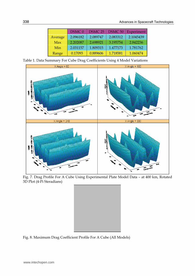
Table 1. Data Summary For Cube Drag Coefficients Using 4 Model Variations
Fig. 7. Drag Profile For A Cube Using Experimental Plate Model Data – at 400 km, Rotated 3D Plot (4-Pi Steradians)
Fig. 8. Maximum Drag Coefficient Profile For A Cube (All Models)
www.intechopen.com

Aerodynamic Disturbance Force and Torque Estimation For Spacecraft and Simple Shapes Using Finite Plate Elements – Part I: Drag Coefficient
339
Fig. 9. Minimum Drag Coefficient Profile For A Cube (DSMC Specularity of 0%)
Fig. 10. Minimum Drag Coefficient Profile For A Cube (Experimental Data; DSMC Specularities 25% and 50%)
3.2 Drag coefficient profile for a cylinder
Using a length to diameter ratio of 2, the drag coefficient profile for a cylinder is determined. The z-axis is aligned with the axis of the cylinder (normal to the circular ends). Figure 11 shows the projected area of the cylinder based upon perspective over 2-pi steradians. Figures 12 through 17 show the drag coefficient data for the cylinder. Figure 12, 16, and 17 display the data using the experimental plate model. Figures 13 through 15 uses DSMC data for specularities of 0%, 25%, and 50% respectively. The maximum drag coefficient occurs with an perspective views are normal to the cylinder ends (z – rotations of 90 and 270 degrees when x – rotation 90 degrees). Therefore, there are 2 potential directions in which the drag coefficient can be maximized for a cylinder. This projected view is shown in Figure 18. Notice that for an x-rotation of 0 degrees the drag coefficient stays constant. This corresponds to the velocity vector being perpendicular to the cylinder’s axis, showing it will be same from any direction perpendicular to this axis, as expected.
www.intechopen.com
Advances in Spacecraft Technologies
340
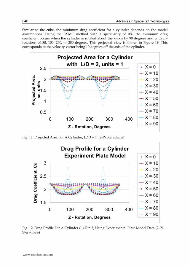
Similar to the cube, the minimum drag coefficient for a cylinder depends on the model assumptions. Using the DSMC method with a specularity of 0%, the minimum drag coefficient occurs when the cylinder is rotated about the x-axis by 90 degrees and with z – rotations of 80, 100, 260, or 280 degrees. This projected view is shown in Figure 19. This corresponds to the velocity vector being 10 degrees off the axis of the cylinder.
Projected Area for a Cylinder
with L/D = 2, units = 1
0.5
1
1.5
2
2.5
0 100 200 300 400
Z - Rotation, Degrees
Pro
jecte
d A
rea,
sq
. u
nit
s
X = 0
X = 10
X = 20
X = 30
X = 40
X = 50
X = 60
X = 70
X = 80
X = 90
Fig. 11. Projected Area For A Cylinder, L/D = 1 (2-Pi Steradians)
Drag Profile for a Cylinder
Experiment Plate Model
1.5
2
2.5
3
0 100 200 300 400
Z - Rotation, Degrees
Dra
g C
oeff
icie
nt,
Cd
X = 0
X = 10
X = 20
X = 30
X = 40
X = 50
X = 60
X = 70
X = 80
X = 90
Fig. 12. Drag Profile For A Cylinder (L/D = 2) Using Experimental Plate Model Data (2-Pi Steradians)
www.intechopen.com
Aerodynamic Disturbance Force and Torque Estimation For Spacecraft and Simple Shapes Using Finite Plate Elements – Part I: Drag Coefficient
341
Drag Profile for a Cylinder
DSMC Method, Specularity = 0%
1.9
1.95
2
2.05
2.1
2.15
2.2
2.25
0 100 200 300 400
Z - Rotation, Degrees
Dra
g C
oe
ffic
ien
t, C
d
X = 0
X = 10
X = 20
X = 30
X = 40
X = 50
X = 60
X = 70
X = 80
X = 90
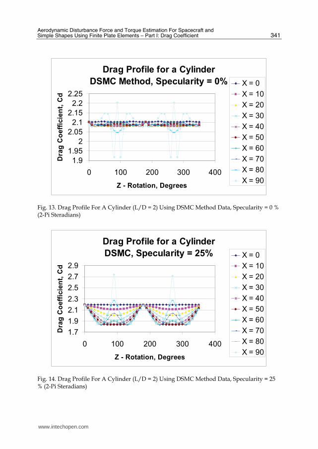
Fig. 13. Drag Profile For A Cylinder (L/D = 2) Using DSMC Method Data, Specularity = 0 % (2-Pi Steradians)
Drag Profile for a Cylinder
DSMC, Specularity = 25%
1.7
1.9
2.1
2.3
2.5
2.7
2.9
0 100 200 300 400
Z - Rotation, Degrees
Dra
g C
oe
ffic
ien
t, C
d
X = 0
X = 10
X = 20
X = 30
X = 40
X = 50
X = 60
X = 70
X = 80
X = 90
Fig. 14. Drag Profile For A Cylinder (L/D = 2) Using DSMC Method Data, Specularity = 25 % (2-Pi Steradians)
www.intechopen.com

Advances in Spacecraft Technologies
342
Drag Profile for a Cylinder
DSMC, Specularity = 50%
1.5
2
2.5
3
3.5
0 100 200 300 400
Z - Rotation, Degrees
Dra
g C
oe
ffic
ien
t, C
d
X = 0
X = 10
X = 20
X = 30
X = 40
X = 50
X = 60
X = 70
X = 80
X = 90
Fig. 15. Drag Profile For A Cylinder (L/D = 2) Using DSMC Method Data, Specularity = 50 % (2-Pi Steradians)
Fig. 16. Drag Profile For A Cylinder (L/D = 2) Using Experimental Plate Model Data, 3D Plot (4-Pi Steradians)
www.intechopen.com
Aerodynamic Disturbance Force and Torque Estimation For Spacecraft and Simple Shapes Using Finite Plate Elements – Part I: Drag Coefficient
343
X Angle = 240 X Angle = 330
X Angle = 60 X Angle = 150
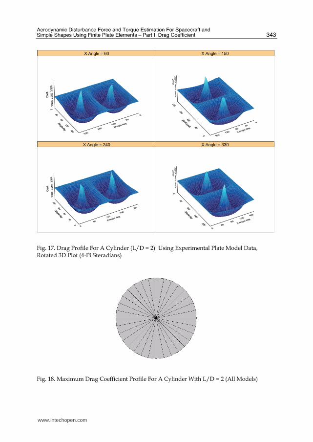
Fig. 17. Drag Profile For A Cylinder (L/D = 2) Using Experimental Plate Model Data, Rotated 3D Plot (4-Pi Steradians)
Fig. 18. Maximum Drag Coefficient Profile For A Cylinder With L/D = 2 (All Models)
www.intechopen.com
Advances in Spacecraft Technologies
344
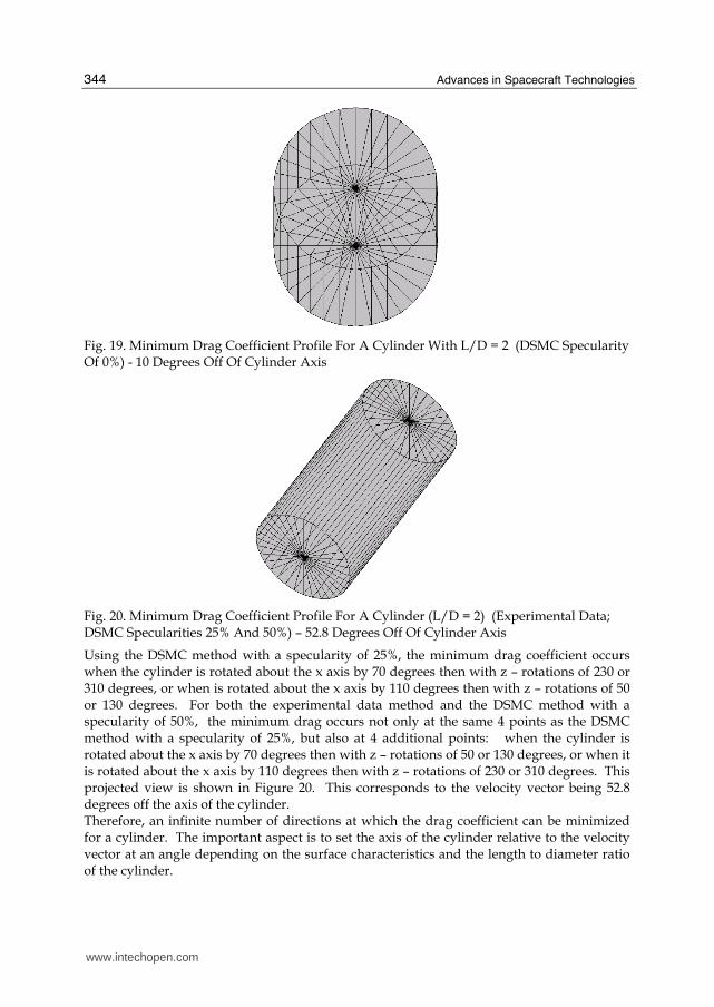
Fig. 19. Minimum Drag Coefficient Profile For A Cylinder With L/D = 2 (DSMC Specularity Of 0%) - 10 Degrees Off Of Cylinder Axis
Fig. 20. Minimum Drag Coefficient Profile For A Cylinder (L/D = 2) (Experimental Data; DSMC Specularities 25% And 50%) – 52.8 Degrees Off Of Cylinder Axis
Using the DSMC method with a specularity of 25%, the minimum drag coefficient occurs when the cylinder is rotated about the x axis by 70 degrees then with z – rotations of 230 or 310 degrees, or when is rotated about the x axis by 110 degrees then with z – rotations of 50 or 130 degrees. For both the experimental data method and the DSMC method with a specularity of 50%, the minimum drag occurs not only at the same 4 points as the DSMC method with a specularity of 25%, but also at 4 additional points: when the cylinder is rotated about the x axis by 70 degrees then with z – rotations of 50 or 130 degrees, or when it is rotated about the x axis by 110 degrees then with z – rotations of 230 or 310 degrees. This projected view is shown in Figure 20. This corresponds to the velocity vector being 52.8 degrees off the axis of the cylinder. Therefore, an infinite number of directions at which the drag coefficient can be minimized for a cylinder. The important aspect is to set the axis of the cylinder relative to the velocity vector at an angle depending on the surface characteristics and the length to diameter ratio of the cylinder.
www.intechopen.com
Aerodynamic Disturbance Force and Torque Estimation For Spacecraft and Simple Shapes Using Finite Plate Elements – Part I: Drag Coefficient
345
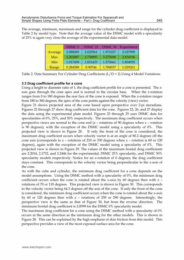
The average, minimum, maximum and range for the cylinder drag coefficient is displayed in Table 2 by model type. Note that the average value of the DSMC model with a specularity of 25% is again very close the average of the experimental data model.
DSMC 0 DSMC 25 DSMC 50 Experiment
Average 2.088085 2.029561 1.971037 2.027999
Max 2.202087 2.738893 3.275698 2.834196
Min 1.917499 1.831433 1.575661 1.804935
Range 0.284588 0.90746 1.700037 1.029261
Table 2. Data Summary For Cylinder Drag Coefficients (L/D = 2) Using 4 Model Variations
3.3 Drag coefficient profile for a cone
Using a height to diameter ratio of 1, the drag coefficient profile for a cone is presented. The z-
axis goes through the cone apex and is normal to the circular base. When the z-rotation
ranges from 0 to 180 degrees the rear face of the cone is exposed. When the z-rotation ranges
from 180 to 360 degrees, the apex of the cone points against the velocity (view) vector.
Figure 21 shows projected area of the cone based upon perspective over 2-pi steradians.
Figures 22 through 27 show drag coefficient data for the cone. Figures 22, 26, and 27 display
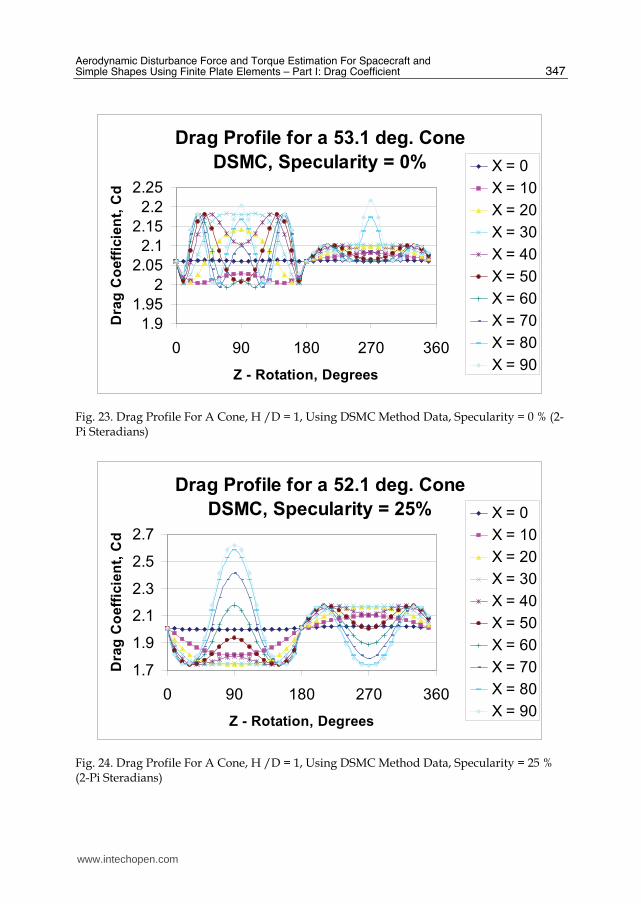
the data using the experimental plate model. Figures 23 through 25 uses DSMC data for
specularities of 0%, 25%, and 50% respectively. The maximum drag coefficient occurs when
perspective views are normal to the cone end (z – rotations of 90 degrees when x – rotation
is 90 degrees), with the exception of the DSMC model using a specularity of 0%. This
projected view is shown in Figure 28. If only the front of the cone is considered, the
maximum drag coefficient occurs when velocity vector is at an angle of 80.2 degrees off the
cone axis (corresponds to z – rotations of 210 or 330 degrees when x – rotation is 60 or 120
degrees), again with the exception of the DSMC model using a specularity of 0%. This
projected view is shown in Figure 29. The values of the maximum frontal drag coefficients
are 2.2014, 2.1732, and 2.2446 for the experimental, DSMC 25% specularity, and DSMC 50%
specularity models respectively. Notice for an x-rotation of 0 degrees, the drag coefficient
stays constant. This corresponds to the velocity vector being perpendicular to the z-axis of
the cone.
As with the cube and cylinder, the minimum drag coefficient for a cone depends on the
model assumptions. Using the DSMC method with a specularity of 0%, the minimum drag
coefficient occurs when the cone is rotated about the x-axis by 60 degrees then with z –
rotations of 70 or 110 degrees. This projected view is shown in Figure 30. This corresponds
to the velocity vector being 64.3 degrees off the axis of the cone. If only the front of the cone
is considered, the minimum drag coefficient occurs when the cone is rotated about the x-axis
by 60 or 120 degrees then with z – rotations of 250 or 290 degrees. Interestingly, the
perspective view is the same as that of Figure 30, but from the reverse direction. The
minimum frontal drag coefficient is 2.0599 for the DSMC 0% specularity model.
The maximum drag coefficient for a cone using the DSMC method with a specularity of 0%
occurs at the same direction as the minimum drag for the other models. This is shown in
Figure 28. This can be explained by the high emphasis of skin friction from this model. This
perspective provides a view of the most exposed surface area for the cone.
www.intechopen.com

Advances in Spacecraft Technologies
346
Projected Area for a 52.1 deg. Cone
(H/D = 1)
0.5
0.55
0.6
0.65
0.7
0.75
0.8
0 90 180 270 360
Z - Rotation, Degrees
Pro
jecte
d A
rea
,
sq
. u
nit
s
X = 0
X = 10
X = 20
X = 30
X = 40
X = 50
X = 60
X = 70
X = 80
X = 90
Fig. 21. Projected Area For A Cone, H/D = 1 (2-Pi Steradians)
Drag Profile for a 53.1 deg. Cone
Experiment Plate Model
1.5
2
2.5
3
0 90 180 270 360
Z - Rotation, Degrees
Dra
g C
oe
ffic
ien
t, C
d
X = 0
X = 10
X = 20
X = 30
X = 40
X = 50
X = 60
X = 70
X = 80
X = 90
Fig. 22. Drag Profile For A Cone, H/D = 1, Using Experimental Plate Model Data (2-Pi Steradians)
www.intechopen.com
Aerodynamic Disturbance Force and Torque Estimation For Spacecraft and Simple Shapes Using Finite Plate Elements – Part I: Drag Coefficient
347
Drag Profile for a 53.1 deg. Cone
DSMC, Specularity = 0%
1.9
1.95
2
2.05
2.1
2.15
2.2
2.25
0 90 180 270 360
Z - Rotation, Degrees
Dra
g C
oe
ffic
ien
t, C
d
X = 0
X = 10
X = 20
X = 30
X = 40
X = 50
X = 60
X = 70
X = 80
X = 90
Fig. 23. Drag Profile For A Cone, H /D = 1, Using DSMC Method Data, Specularity = 0 % (2-Pi Steradians)
Drag Profile for a 52.1 deg. Cone
DSMC, Specularity = 25%
1.7
1.9
2.1
2.3
2.5
2.7
0 90 180 270 360
Z - Rotation, Degrees
Dra
g C
oe
ffic
ien
t, C
d
X = 0
X = 10
X = 20
X = 30
X = 40
X = 50
X = 60
X = 70
X = 80
X = 90
Fig. 24. Drag Profile For A Cone, H /D = 1, Using DSMC Method Data, Specularity = 25 % (2-Pi Steradians)
www.intechopen.com
Advances in Spacecraft Technologies
348
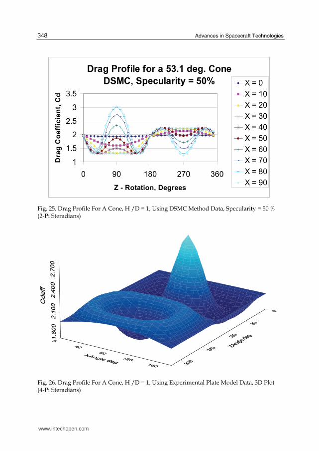
Drag Profile for a 53.1 deg. Cone
DSMC, Specularity = 50%
1
1.5
2
2.5
3
3.5
0 90 180 270 360
Z - Rotation, Degrees
Dra
g C
oe
ffic
ien
t, C
d
X = 0
X = 10
X = 20
X = 30
X = 40
X = 50
X = 60
X = 70
X = 80
X = 90
Fig. 25. Drag Profile For A Cone, H /D = 1, Using DSMC Method Data, Specularity = 50 % (2-Pi Steradians)
Fig. 26. Drag Profile For A Cone, H /D = 1, Using Experimental Plate Model Data, 3D Plot (4-Pi Steradians)
www.intechopen.com

Aerodynamic Disturbance Force and Torque Estimation For Spacecraft and Simple Shapes Using Finite Plate Elements – Part I: Drag Coefficient
349
X Angle = 313 X Angle = 43
X Angle = 133 X Angle = 223
Fig. 27. Drag Profile For A Cone, (H /D = 1) Using Experimental Plate Model Data, Rotated 3D Plot (4-Pi Steradians)
Fig. 28. Minimum And Maximum Drag Coefficient Profile For A Cone With H/D = 1 (All Models Except DSMC Specularity 0% For Minimum Drag Coefficient)
Fig. 29. Maximum Drag Coefficient Profile (Frontal Direction Only) For A Cone With H/D = 1 (Experimental Data; DSMC Specularities 25% And 50%) – 80.2 Degrees Off Of Cone Axis
www.intechopen.com
Advances in Spacecraft Technologies
350
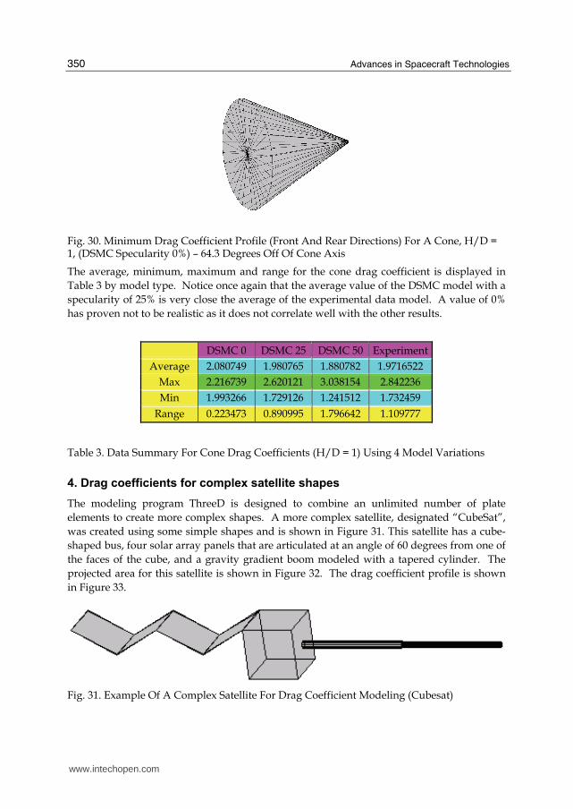
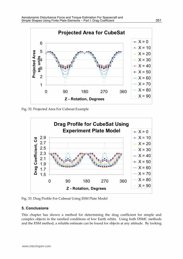
Fig. 30. Minimum Drag Coefficient Profile (Front And Rear Directions) For A Cone, H/D = 1, (DSMC Specularity 0%) – 64.3 Degrees Off Of Cone Axis
The average, minimum, maximum and range for the cone drag coefficient is displayed in
Table 3 by model type. Notice once again that the average value of the DSMC model with a
specularity of 25% is very close the average of the experimental data model. A value of 0%
has proven not to be realistic as it does not correlate well with the other results.
DSMC 0 DSMC 25 DSMC 50 Experiment
Average 2.080749 1.980765 1.880782 1.9716522
Max 2.216739 2.620121 3.038154 2.842236
Min 1.993266 1.729126 1.241512 1.732459
Range 0.223473 0.890995 1.796642 1.109777
Table 3. Data Summary For Cone Drag Coefficients (H/D = 1) Using 4 Model Variations
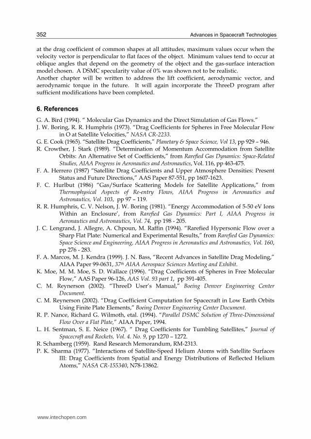
4. Drag coefficients for complex satellite shapes
The modeling program ThreeD is designed to combine an unlimited number of plate
elements to create more complex shapes. A more complex satellite, designated “CubeSat”,
was created using some simple shapes and is shown in Figure 31. This satellite has a cube-
shaped bus, four solar array panels that are articulated at an angle of 60 degrees from one of
the faces of the cube, and a gravity gradient boom modeled with a tapered cylinder. The
projected area for this satellite is shown in Figure 32. The drag coefficient profile is shown
in Figure 33.
Fig. 31. Example Of A Complex Satellite For Drag Coefficient Modeling (Cubesat)
www.intechopen.com
Aerodynamic Disturbance Force and Torque Estimation For Spacecraft and Simple Shapes Using Finite Plate Elements – Part I: Drag Coefficient
351
Projected Area for CubeSat
1
2
3
4
5
6
0 90 180 270 360
Z - Rotation, Degrees
Pro
jec
ted
Are
a
sq
. u
nit
sX = 0
X = 10
X = 20
X = 30
X = 40
X = 50
X = 60
X = 70
X = 80
X = 90
Fig. 32. Projected Area For Cubesat Example
Drag Profile for CubeSat Using
Experiment Plate Model
1.5
1.7
1.9
2.1
2.3
2.5
2.7
2.9
0 90 180 270 360
Z - Rotation, Degrees
Dra
g C
oeff
icie
nt,
Cd
X = 0
X = 10
X = 20
X = 30
X = 40
X = 50
X = 60
X = 70
X = 80
X = 90
Fig. 33. Drag Profile For Cubesat Using ESM Plate Model
5. Conclusions
This chapter has shown a method for determining the drag coefficient for simple and complex objects in the rarefied conditions of low Earth orbits. Using both DSMC methods and the ESM method, a reliable estimate can be found for objects at any attitude. By looking
www.intechopen.com
Advances in Spacecraft Technologies
352
at the drag coefficient of common shapes at all attitudes, maximum values occur when the velocity vector is perpendicular to flat faces of the object. Minimum values tend to occur at oblique angles that depend on the geometry of the object and the gas-surface interaction model chosen. A DSMC specularity value of 0% was shown not to be realistic. Another chapter will be written to address the lift coefficient, aerodynamic vector, and aerodynamic torque in the future. It will again incorporate the ThreeD program after sufficient modifications have been completed.
6. References
G. A. Bird (1994). “ Molecular Gas Dynamics and the Direct Simulation of Gas Flows.” J. W. Boring, R. R. Humphris (1973). “Drag Coefficients for Spheres in Free Molecular Flow
in O at Satellite Velocities,” NASA CR-2233. G. E. Cook (1965). “Satellite Drag Coefficients,” Planetary & Space Science, Vol 13, pp 929 – 946. R. Crowther, J. Stark (1989). “Determination of Momentum Accommodation from Satellite
Orbits: An Alternative Set of Coefficients,” from Rarefied Gas Dynamics: Space-Related Studies, AIAA Progress in Aeronautics and Astronautics, Vol. 116, pp 463-475.
F. A. Herrero (1987) “Satellite Drag Coefficients and Upper Atmosphere Densities: Present Status and Future Directions,” AAS Paper 87-551, pp 1607-1623.
F. C. Hurlbut (1986) “Gas/Surface Scattering Models for Satellite Applications,” from Thermophysical Aspects of Re-entry Flows, AIAA Progress in Aeronautics and Astronautics, Vol. 103, pp 97 – 119.
R. R. Humphris, C. V. Nelson, J. W. Boring (1981). “Energy Accommodation of 5-50 eV Ions Within an Enclosure’, from Rarefied Gas Dynamics: Part I, AIAA Progress in Aeronautics and Astronautics, Vol. 74, pp 198 - 205.
J. C. Lengrand, J. Allegre, A. Chpoun, M. Raffin (1994). “Rarefied Hypersonic Flow over a Sharp Flat Plate: Numerical and Experimental Results,” from Rarefied Gas Dynamics: Space Science and Engineering, AIAA Progress in Aeronautics and Astronautics, Vol. 160, pp 276 - 283.
F. A. Marcos, M. J. Kendra (1999). J. N. Bass, “Recent Advances in Satellite Drag Modeling,” AIAA Paper 99-0631, 37th AIAA Aerospace Sciences Meeting and Exhibit.
K. Moe, M. M. Moe, S. D. Wallace (1996). “Drag Coefficients of Spheres in Free Molecular Flow,” AAS Paper 96-126, AAS Vol. 93 part 1, pp 391-405.
C. M. Reynerson (2002). “ThreeD User’s Manual,” Boeing Denver Engineering Center Document.
C. M. Reynerson (2002). “Drag Coefficient Computation for Spacecraft in Low Earth Orbits Using Finite Plate Elements,” Boeing Denver Engineering Center Document.
R. P. Nance, Richard G. Wilmoth, etal. (1994). “Parallel DSMC Solution of Three-Dimensional Flow Over a Flat Plate,” AIAA Paper, 1994.
L. H. Sentman, S. E. Neice (1967). “ Drag Coefficients for Tumbling Satellites,” Journal of Spacecraft and Rockets, Vol. 4. No. 9, pp 1270 – 1272.
R. Schamberg (1959). Rand Research Memorandum, RM-2313. P. K. Sharma (1977). “Interactions of Satellite-Speed Helium Atoms with Satellite Surfaces
III: Drag Coefficients from Spatial and Energy Distributions of Reflected Helium Atoms,” NASA CR-155340, N78-13862.
www.intechopen.com

Advances in Spacecraft TechnologiesEdited by Dr Jason Hall
ISBN 978-953-307-551-8Hard cover, 596 pagesPublisher InTechPublished online 14, February, 2011Published in print edition February, 2011
InTech EuropeUniversity Campus STeP Ri Slavka Krautzeka 83/A 51000 Rijeka, Croatia Phone: +385 (51) 770 447 Fax: +385 (51) 686 166www.intechopen.com
InTech ChinaUnit 405, Office Block, Hotel Equatorial Shanghai No.65, Yan An Road (West), Shanghai, 200040, China
Phone: +86-21-62489820 Fax: +86-21-62489821
The development and launch of the first artificial satellite Sputnik more than five decades ago propelled boththe scientific and engineering communities to new heights as they worked together to develop novel solutionsto the challenges of spacecraft system design. This symbiotic relationship has brought significant technologicaladvances that have enabled the design of systems that can withstand the rigors of space while providingvaluable space-based services. With its 26 chapters divided into three sections, this book brings togethercritical contributions from renowned international researchers to provide an outstanding survey of recentadvances in spacecraft technologies. The first section includes nine chapters that focus on innovativehardware technologies while the next section is comprised of seven chapters that center on cutting-edge stateestimation techniques. The final section contains eleven chapters that present a series of novel controlmethods for spacecraft orbit and attitude control.
How to referenceIn order to correctly reference this scholarly work, feel free to copy and paste the following:
Charles Reynerson (2011). Aerodynamic Disturbance Force and Torque Estimation for Spacecraft and SimpleShapes Using Finite Plate Elements – Part I: Drag Coefficient, Advances in Spacecraft Technologies, Dr JasonHall (Ed.), ISBN: 978-953-307-551-8, InTech, Available from: http://www.intechopen.com/books/advances-in-spacecraft-technologies/aerodynamic-disturbance-force-and-torque-estimation-for-spacecraft-and-simple-shapes-using-finite-pl

© 2011 The Author(s). Licensee IntechOpen. This chapter is distributedunder the terms of the Creative Commons Attribution-NonCommercial-ShareAlike-3.0 License, which permits use, distribution and reproduction fornon-commercial purposes, provided the original is properly cited andderivative works building on this content are distributed under the samelicense.