Aerodynamic Shape Optimization of a Blended-Wing …oddjob.utias.utoronto.ca/dwz/Miscellaneous/Reist2013-2414.pdfBlended-Wing-Body Regional Transport ... system on the top of the aircraft

Aerodynamic Shape Optimization of a

Blended-Wing-Body Regional Transport

for a Short Range Mission

Thomas A. Reist∗ and David W. Zingg†

Institute for Aerospace Studies, University of Toronto

4925 Dufferin St., Toronto, Ontario, M3H 5T6, Canada

The blended-wing-body represents a potential revolution in efficient aircraft design. Alift-constrained drag-minimization optimization problem is solved for the optimal shapeof a blended-wing-body transonic regional jet. A Newton-Krylov solver for the Eulerand Reynolds-Averaged Navier-Stokes (RANS) equations is coupled with a gradient-basedoptimizer, where gradients are calculated via the discrete adjoint method. A 98-passengerregional jet is optimized for a 500nmi mission at 40,000ft and Mach 0.8. A series ofsingle and multipoint optimization problems using both the Euler and RANS equations areconsidered in order to examine the trade-offs between the imposition of different constraintsincluding trim and longitudinal static stability. Drag reductions of up to 55% and 38%are achieved for the Euler and RANS-based optimizations respectively. In each case anelliptical lift distribution is attained on the wing, shocks are eliminated, and in the RANS-based optimization the large regions of highly separated flow on the baseline design aregreatly reduced. These drag reductions are achieved while both trimming and stabilizingthe baseline design.

Nomenclature

x, y, z Stream-wise, span-wise and vertical coordinatesb Total aircraft semi-spanc Local chord lengthcroot Chord length at the aircraft center-lineMAC Mean aerodynamic chordS Reference planform areat/c Section thickness normalized with local chord lengthCL, CD, CM Lift, drag and pitching moment coefficients of the entire aircraftAoA Angle-of-attackM Freestream Mach numberq∞ Freestream dynamic pressurea Sound speed at cruise conditionsW Aircraft weightMTOW Maximum take-off weightOEW Operating empty weightcT Thrust specific fuel consumptionKn Static margin as percent of the MAC∆CG Center of gravity perturbation design variable

∗Ph.D. Candidate, AIAA Student member, [email protected]†Professor and Director, Canada Research Chair in Computational Aerodynamics and Environmentally Friendly Aircraft

Design, J. Armand Bombardier Foundation Chair in Aerospace Flight, Associate Fellow AIAA, [email protected]

1 of 14

American Institute of Aeronautics and Astronautics

Dow

nloa

ded

by D

avid

Zin

gg o

n Ju

ly 2

, 201

3 | h

ttp://

arc.

aiaa

.org

| D

OI:

10.

2514

/6.2

013-

2414

31st AIAA Applied Aerodynamics Conference

June 24-27, 2013, San Diego, CA

AIAA 2013-2414

Copyright © 2013 by Thomas A. Reist and David W. Zingg. Published by the American Institute of Aeronautics and Astronautics, Inc., with permission.

I. Introduction

With increasing oil prices and concern about both the exhaustion of fossil fuels and their contribution toclimate change, the need for more fuel efficient aircraft is becoming more pronounced for both economic

and environmental reasons. Although there have been great advances in transport aircraft efficiency sincethe introduction of the de Havilland Comet in 1952, the conventional tube-wing configuration remains tothis day. Performance improvements have come from modifications to aerodynamic design, such as the useof winglets and supercritical airfoils, as well as high performance materials and increasingly fuel efficientengines. However a step change in fuel efficiency may be realized through novel configurations. One suchconfiguration that has received much attention in recent years is the blended-wing-body (BWB). This designcombines the aircraft fuselage and wings into one tightly integrated airframe with improved aerodynamic,structural, propulsive, and acoustic efficiency.

The BWB has the potential to be more aerodynamically efficient than conventional configurations forseveral reasons. For a given internal volume, the BWB has less wetted surface area, leading to a betterlift-to-drag ratio.1 It has also been shown to be more area-ruled than conventional designs, which allows forreduced wave drag and potentially higher cruise speeds.1 The overall shape of the BWB is also cleaner thana conventional design, leading to reduced interference drag. Structurally, the aerodynamic lifting loads aremore closely aligned with the weight of the aircraft due to the lifting fuselage, leading to reduced bending loadsin the main wing structure and therefore lower structural weight.1 The use of a well integrated propulsionsystem, such as boundary-layer-ingestion or distributed propulsion, can lead to propulsive efficiencies. Awell integrated propulsion system on the top of the aircraft can also provide significant noise reductions dueto the acoustic shielding provided by the aerodynamic surfaces.2 The highly integrated nature of the designallows for efficiency improvements; however this also increases the design challenges stemming from such ahighly coupled configuration.

One of the main structural challenges associated with the BWB is the lack of the efficient cylindricalpressure vessel present in conventional designs. Much work has been dedicated to the design of efficientcomposite structures tailored for handling these pressure loads.3–5 Due to its tailless nature, stability andcontrol can be challenging with this design. Work has been done on addressing some of these issues.6,7 Withsuch a radically different design, certification and customer acceptance must also be addressed. Finally,perhaps the biggest obstacle to the development of the BWB is the financial risk associated with pursuingsuch a novel design. However, as rising fuel prices continue to reduce operating profits, the potential benefitsof this unconventional design may justify its development.

Several large projects around the world have focused on the development of the BWB design. In theUnited States, Boeing and NASA have been involved in the identification and development of enabling tech-nologies required for the BWB design,1,3, 6, 8–10 with contributions leading to the X-48 flight demonstrators.A BWB design focused on noise reduction has been developed as part of Cambridge and MIT’s ‘Silent’Aircraft Initiative.2,11 In Europe, two of the main projects relating to BWB design are the MultidisciplinaryOptimization of a Blended Wing Body (MOB)12 and the Very Efficient Large Aircraft (VELA)13 projects.

Aerodynamic shape optimization (ASO) has been applied to the BWB design at a variety of fidelitylevels. Peigin and Epstein14 used a Navier-Stokes solver and genetic optimizer for the optimization of theMOB configuration for multiple operating points with airfoil, dihedral and twist design variables. Qin etal.15 performed spanload optimization through twist modification as well as 3D surface optimization usingboth Euler and Navier-Stokes solvers. Both airfoil and sweep optimization were performed by Le Moigneand Qin16 using a discrete adjoint method with an Euler solver. They demonstrated that the imposition ofpitching moment constraints has a large impact on the optimal shape yet only a small performance penaltymust be paid. The performance improvements obtained using Euler-based optimization are also realizedwhen evaluated with a Navier-Stokes solver. A small BWB was optimized by Kuntawala et al.17 using alarge number of geometric design variables for full 3D surface optimization.

Historically, the focus of BWB design investigations has been on large capacity aircraft in the 400-1000passenger range. The BWB’s intrinsic design features lend themselves well to large aircraft. However thisdesign may also offer advantages in the regional jet segment. Nickol examined a series of BWB aircraftranging from 98-400 passengers.9 As expected, the fuel burn benefit was most significant for the largeraircraft, with the 98 passenger aircraft burning more fuel than a comparable tube-wing aircraft. However,the fuel burn disadvantage of the small BWB was highly sensitive to drag. Thus, if a suitable drag reductioncan be achieved through aerodynamic shape optimization, the BWB could potentially be more fuel efficientthan the tube-wing aircraft for a variety of aircraft classes.

2 of 14


Dow

nloa

ded

by D

avid

Zin

gg o

n Ju

ly 2

, 201

3 | h

ttp://

arc.

aiaa

.org

| D

OI:

10.

2514

/6.2

013-

2414


II. Optimization Methodology

The aerodynamic shape optimization algorithm used comprises three main components: 1) a multiblockNewton-Krylov solver for the Euler and Reynolds-Averaged Navier-Stokes (RANS) equations, 2) a B-splinegeometry parameterization which is coupled with a linear elasticity mesh movement strategy, and 3) thegradient-based optimizer SNOPT with gradients calculated using the discrete adjoint method.

The flow solver is a multiblock finite-difference solver which uses summation-by-parts operators for spatialdiscretization and simultaneous approximation terms for the imposition of boundary conditions and blockinterface conditions. The Krylov subspace method Generalized Minimum Residual (GMRES) is used withapproximate Schur preconditioning for the solution of the discrete equations. The one-equation Spalart-Allmaras turbulence model is used for the modeling of turbulent flows. Details of the flow solver can befound in Hicken and Zingg18 and Osusky and Zingg.19

At each optimization iteration for which a geometric shape change occurs, the computational grid mustbe moved to reflect this change. To accomplish this, each block of the computational grid is fitted with aB-spline volume. As the B-spline control points on the aerodynamic surface are moved by the optimizer, eachB-spline volume block is treated as a linear elastic solid, for which a finite-element solution is obtained todefine the new shape of the B-spline volume. The computational grid is then recovered from this new B-splinevolume. This method has been found to be very robust for large shape changes while being computationallyinexpensive. Details can be found in Hicken and Zingg.20

Due to the high cost of evaluating the flow equations, a gradient-based optimizer is used for optimization,as gradient-based optimizers typically require fewer function evaluations than genetic algorithms.21 Thepenalty paid is that for multimodal optimization problems only a local optimum may be found. This canbe addressed using the gradient-based global optimization techniques proposed by Chernukhin and Zingg.22

The gradients of the objective and constraints are evaluated using the discrete adjoint method. This methodis advantageous for problems with many design variables, as the cost of the gradient evaluation is nearlyindependent of the number of design variables. The gradient-based optimizer SNOPT is used, as it allows forthe solution of large-scale constrained problems. Details of the adjoint method and its integration with theflow solver and mesh movement are given by Hicken and Zingg20 while the details of SNOPT are describedby Gill et al.23

The above algorithm has been used extensively for ASO of various wing geometries including induceddrag minimization of non-planar wings,24 optimization of wings in turbulent flows,25 the investigation of themultimodality of ASO problems22 and the optimization of BWB aircraft.17

III. Baseline Design

The aircraft considered in this work is intended to serve as a regional jet with a single-class capacityof approximately 100 passengers and four crew, while having a maximum range capability of 2000nmi with100nmi reserves. The first step in generating a geometric shape is to size the cabin such that it fits allpassengers, crew, aisles and monuments (such as lavatories and galleys) so as to produce a shape that canbe well integrated into the rest of the airframe in order to avoid unnecessary structural weight, while at thesame time providing a pressure vessel shape that is as efficient as possible. As in many BWB concepts1,2, 9, 26

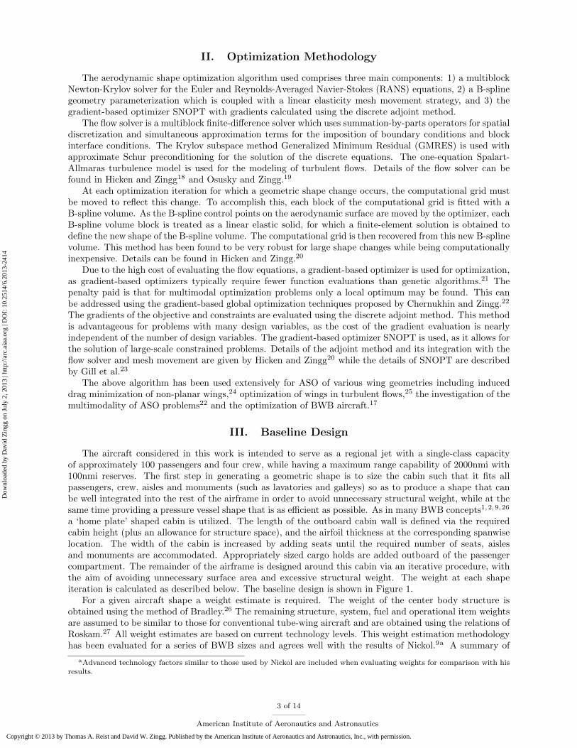
a ‘home plate’ shaped cabin is utilized. The length of the outboard cabin wall is defined via the requiredcabin height (plus an allowance for structure space), and the airfoil thickness at the corresponding spanwiselocation. The width of the cabin is increased by adding seats until the required number of seats, aislesand monuments are accommodated. Appropriately sized cargo holds are added outboard of the passengercompartment. The remainder of the airframe is designed around this cabin via an iterative procedure, withthe aim of avoiding unnecessary surface area and excessive structural weight. The weight at each shapeiteration is calculated as described below. The baseline design is shown in Figure 1.

For a given aircraft shape a weight estimate is required. The weight of the center body structure isobtained using the method of Bradley.26 The remaining structure, system, fuel and operational item weightsare assumed to be similar to those for conventional tube-wing aircraft and are obtained using the relations ofRoskam.27 All weight estimates are based on current technology levels. This weight estimation methodologyhas been evaluated for a series of BWB sizes and agrees well with the results of Nickol.9a A summary of

aAdvanced technology factors similar to those used by Nickol are included when evaluating weights for comparison with hisresults.

3 of 14


Dow

nloa

ded

by D

avid

Zin

gg o

n Ju

ly 2

, 201

3 | h

ttp://

arc.

aiaa

.org

| D

OI:

10.

2514

/6.2

013-

2414


Car

go

Car

go

M M

C.G. location

M

Wing box

Monument

Figure 1: Baseline design with passenger layout andwingbox structure.

CapacityPassengers 98Crew 4Cabin floor area 593 ft2

Cargo volume 685 ft3

GeometryPlanform area 2177 ft2

Total span 90 ftLength 74 ftMAC 44 ftAspect ratio 3.7

WeightMTOW 96,760 lbOEW 54,710 lbPayload 23,380 lbWing load at MTOW 44 lb/ft2

Cruise conditionsDesign range 500 nmiAltitude 40,000 ftReynolds number* 70 ×106

Mach number 0.80xCG/croot 0.65

* Based on full aircraft MAC.

Table 1: Baseline design summary.

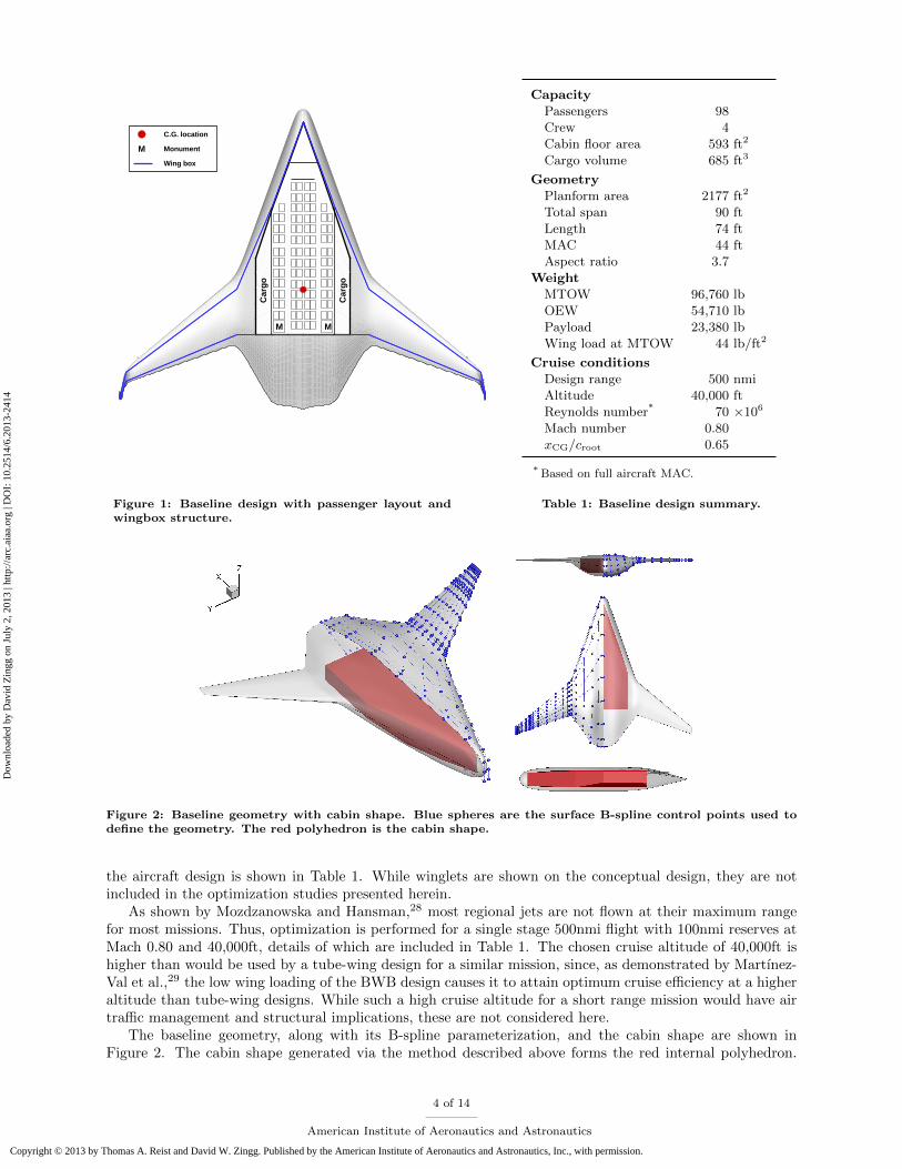
Figure 2: Baseline geometry with cabin shape. Blue spheres are the surface B-spline control points used todefine the geometry. The red polyhedron is the cabin shape.

the aircraft design is shown in Table 1. While winglets are shown on the conceptual design, they are notincluded in the optimization studies presented herein.

As shown by Mozdzanowska and Hansman,28 most regional jets are not flown at their maximum rangefor most missions. Thus, optimization is performed for a single stage 500nmi flight with 100nmi reserves atMach 0.80 and 40,000ft, details of which are included in Table 1. The chosen cruise altitude of 40,000ft ishigher than would be used by a tube-wing design for a similar mission, since, as demonstrated by Martınez-Val et al.,29 the low wing loading of the BWB design causes it to attain optimum cruise efficiency at a higheraltitude than tube-wing designs. While such a high cruise altitude for a short range mission would have airtraffic management and structural implications, these are not considered here.

The baseline geometry, along with its B-spline parameterization, and the cabin shape are shown inFigure 2. The cabin shape generated via the method described above forms the red internal polyhedron.

4 of 14


Dow

nloa

ded

by D

avid

Zin

gg o

n Ju

ly 2

, 201

3 | h

ttp://

arc.

aiaa

.org

| D

OI:

10.

2514

/6.2

013-

2414


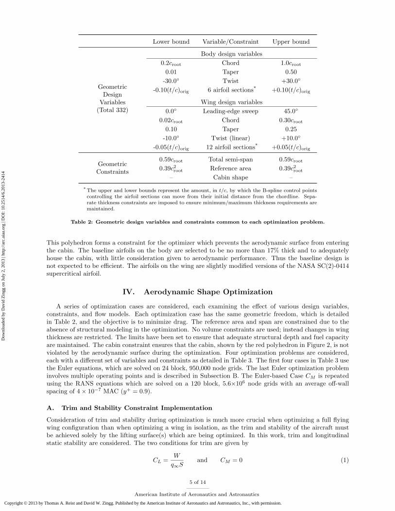
Lower bound Variable/Constraint Upper bound

GeometricDesign

Variables(Total 332)

Body design variables

0.2croot Chord 1.0croot

0.01 Taper 0.50

-30.0◦ Twist +30.0◦

-0.10(t/c)orig 6 airfoil sections* +0.10(t/c)orig

Wing design variables

0.0◦ Leading-edge sweep 45.0◦

0.02croot Chord 0.30croot

0.10 Taper 0.25

-10.0◦ Twist (linear) +10.0◦

-0.05(t/c)orig 12 airfoil sections* +0.05(t/c)orig

GeometricConstraints

0.59croot Total semi-span 0.59croot

0.39c2root Reference area 0.39c2

root

– Cabin shape –

* The upper and lower bounds represent the amount, in t/c, by which the B-spline control pointscontrolling the airfoil sections can move from their initial distance from the chordline. Sepa-rate thickness constraints are imposed to ensure minimum/maximum thickness requirements aremaintained.

Table 2: Geometric design variables and constraints common to each optimization problem.

This polyhedron forms a constraint for the optimizer which prevents the aerodynamic surface from enteringthe cabin. The baseline airfoils on the body are selected to be no more than 17% thick and to adequatelyhouse the cabin, with little consideration given to aerodynamic performance. Thus the baseline design isnot expected to be efficient. The airfoils on the wing are slightly modified versions of the NASA SC(2)-0414supercritical airfoil.

IV. Aerodynamic Shape Optimization

A series of optimization cases are considered, each examining the effect of various design variables,constraints, and flow models. Each optimization case has the same geometric freedom, which is detailedin Table 2, and the objective is to minimize drag. The reference area and span are constrained due to theabsence of structural modeling in the optimization. No volume constraints are used; instead changes in wingthickness are restricted. The limits have been set to ensure that adequate structural depth and fuel capacityare maintained. The cabin constraint ensures that the cabin, shown by the red polyhedron in Figure 2, is notviolated by the aerodynamic surface during the optimization. Four optimization problems are considered,each with a different set of variables and constraints as detailed in Table 3. The first four cases in Table 3 usethe Euler equations, which are solved on 24 block, 950,000 node grids. The last Euler optimization probleminvolves multiple operating points and is described in Subsection B. The Euler-based Case CM is repeatedusing the RANS equations which are solved on a 120 block, 5.6×106 node grids with an average off-wallspacing of 4 × 10−7 MAC (y+ = 0.9).

A. Trim and Stability Constraint Implementation

Consideration of trim and stability during optimization is much more crucial when optimizing a full flyingwing configuration than when optimizing a wing in isolation, as the trim and stability of the aircraft mustbe achieved solely by the lifting surface(s) which are being optimized. In this work, trim and longitudinalstatic stability are considered. The two conditions for trim are given by

CL =W

q∞Sand CM = 0 (1)

5 of 14


Dow

nloa

ded

by D

avid

Zin

gg o

n Ju

ly 2

, 201

3 | h

ttp://

arc.

aiaa

.org

| D

OI:

10.

2514

/6.2

013-

2414


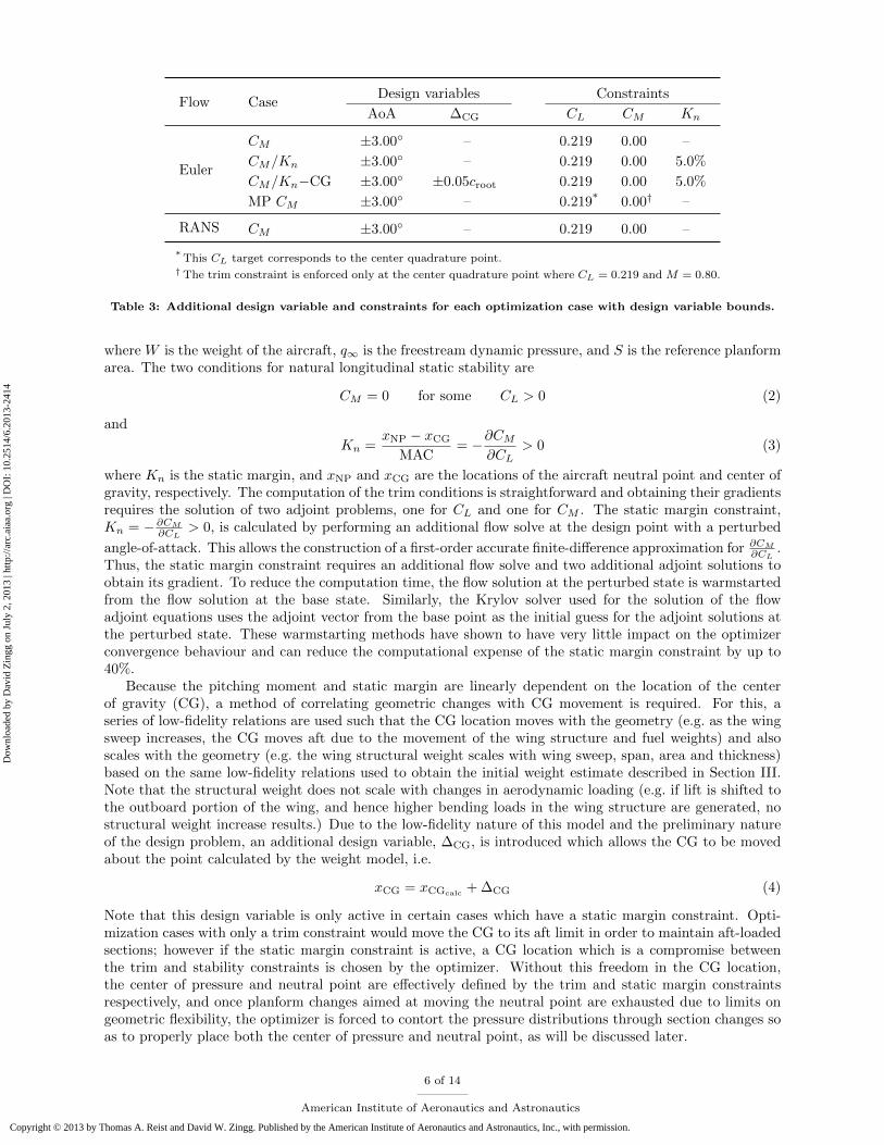
Flow CaseDesign variables Constraints

AoA ∆CG CL CM Kn

Euler

CM ±3.00◦ – 0.219 0.00 –

CM/Kn ±3.00◦ – 0.219 0.00 5.0%

CM/Kn−CG ±3.00◦ ±0.05croot 0.219 0.00 5.0%

MP CM ±3.00◦ – 0.219* 0.00† –

RANS CM ±3.00◦ – 0.219 0.00 –

* This CL target corresponds to the center quadrature point.†The trim constraint is enforced only at the center quadrature point where CL = 0.219 and M = 0.80.

Table 3: Additional design variable and constraints for each optimization case with design variable bounds.

where W is the weight of the aircraft, q∞ is the freestream dynamic pressure, and S is the reference planformarea. The two conditions for natural longitudinal static stability are

CM = 0 for some CL > 0 (2)

and

Kn =xNP − xCG

MAC= −∂CM

∂CL> 0 (3)

where Kn is the static margin, and xNP and xCG are the locations of the aircraft neutral point and center ofgravity, respectively. The computation of the trim conditions is straightforward and obtaining their gradientsrequires the solution of two adjoint problems, one for CL and one for CM . The static margin constraint,Kn = −∂CM

∂CL> 0, is calculated by performing an additional flow solve at the design point with a perturbed

angle-of-attack. This allows the construction of a first-order accurate finite-difference approximation for ∂CM

∂CL.

Thus, the static margin constraint requires an additional flow solve and two additional adjoint solutions toobtain its gradient. To reduce the computation time, the flow solution at the perturbed state is warmstartedfrom the flow solution at the base state. Similarly, the Krylov solver used for the solution of the flowadjoint equations uses the adjoint vector from the base point as the initial guess for the adjoint solutions atthe perturbed state. These warmstarting methods have shown to have very little impact on the optimizerconvergence behaviour and can reduce the computational expense of the static margin constraint by up to40%.

Because the pitching moment and static margin are linearly dependent on the location of the centerof gravity (CG), a method of correlating geometric changes with CG movement is required. For this, aseries of low-fidelity relations are used such that the CG location moves with the geometry (e.g. as the wingsweep increases, the CG moves aft due to the movement of the wing structure and fuel weights) and alsoscales with the geometry (e.g. the wing structural weight scales with wing sweep, span, area and thickness)based on the same low-fidelity relations used to obtain the initial weight estimate described in Section III.Note that the structural weight does not scale with changes in aerodynamic loading (e.g. if lift is shifted tothe outboard portion of the wing, and hence higher bending loads in the wing structure are generated, nostructural weight increase results.) Due to the low-fidelity nature of this model and the preliminary natureof the design problem, an additional design variable, ∆CG, is introduced which allows the CG to be movedabout the point calculated by the weight model, i.e.

xCG = xCGcalc+ ∆CG (4)

Note that this design variable is only active in certain cases which have a static margin constraint. Opti-mization cases with only a trim constraint would move the CG to its aft limit in order to maintain aft-loadedsections; however if the static margin constraint is active, a CG location which is a compromise betweenthe trim and stability constraints is chosen by the optimizer. Without this freedom in the CG location,the center of pressure and neutral point are effectively defined by the trim and static margin constraintsrespectively, and once planform changes aimed at moving the neutral point are exhausted due to limits ongeometric flexibility, the optimizer is forced to contort the pressure distributions through section changes soas to properly place both the center of pressure and neutral point, as will be discussed later.

6 of 14


Dow

nloa

ded

by D

avid

Zin

gg o

n Ju

ly 2

, 201

3 | h

ttp://

arc.

aiaa

.org

| D

OI:

10.

2514

/6.2

013-

2414


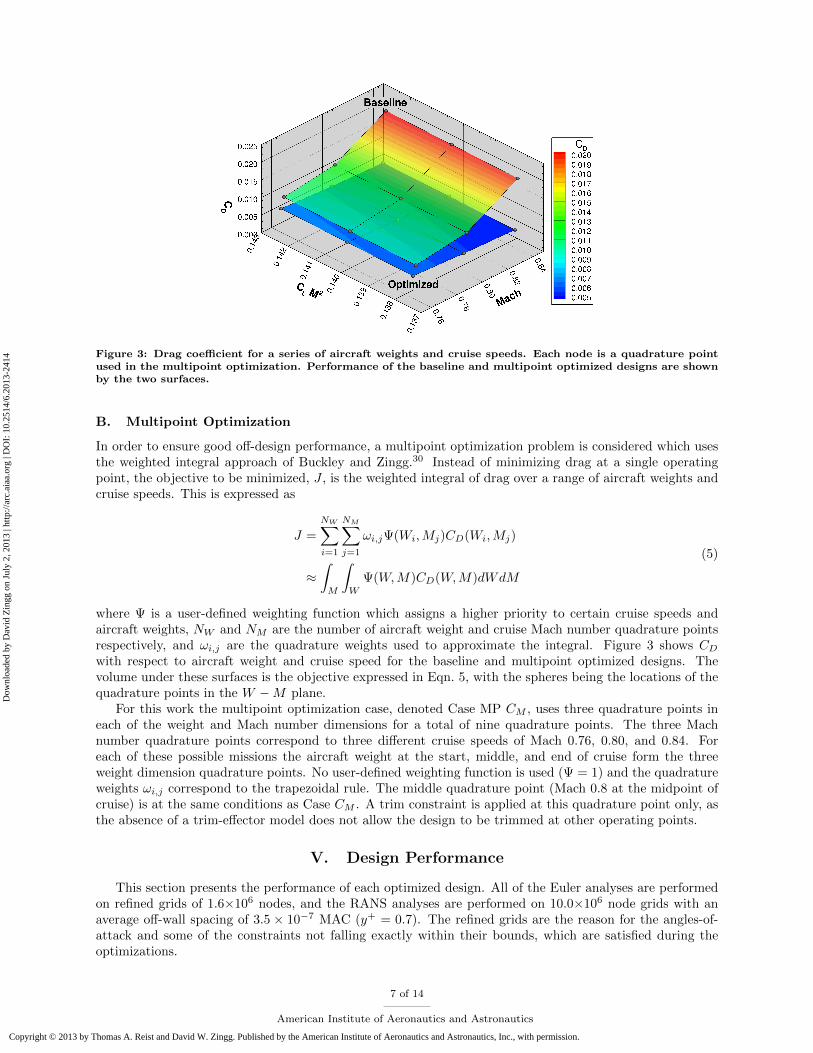
Figure 3: Drag coefficient for a series of aircraft weights and cruise speeds. Each node is a quadrature pointused in the multipoint optimization. Performance of the baseline and multipoint optimized designs are shownby the two surfaces.

B. Multipoint Optimization

In order to ensure good off-design performance, a multipoint optimization problem is considered which usesthe weighted integral approach of Buckley and Zingg.30 Instead of minimizing drag at a single operatingpoint, the objective to be minimized, J , is the weighted integral of drag over a range of aircraft weights andcruise speeds. This is expressed as

J =

NW∑i=1

NM∑j=1

ωi,jΨ(Wi,Mj)CD(Wi,Mj)

≈∫M

∫W

Ψ(W,M)CD(W,M)dWdM

(5)

where Ψ is a user-defined weighting function which assigns a higher priority to certain cruise speeds andaircraft weights, NW and NM are the number of aircraft weight and cruise Mach number quadrature pointsrespectively, and ωi,j are the quadrature weights used to approximate the integral. Figure 3 shows CD

with respect to aircraft weight and cruise speed for the baseline and multipoint optimized designs. Thevolume under these surfaces is the objective expressed in Eqn. 5, with the spheres being the locations of thequadrature points in the W −M plane.

For this work the multipoint optimization case, denoted Case MP CM , uses three quadrature points ineach of the weight and Mach number dimensions for a total of nine quadrature points. The three Machnumber quadrature points correspond to three different cruise speeds of Mach 0.76, 0.80, and 0.84. Foreach of these possible missions the aircraft weight at the start, middle, and end of cruise form the threeweight dimension quadrature points. No user-defined weighting function is used (Ψ = 1) and the quadratureweights ωi,j correspond to the trapezoidal rule. The middle quadrature point (Mach 0.8 at the midpoint ofcruise) is at the same conditions as Case CM . A trim constraint is applied at this quadrature point only, asthe absence of a trim-effector model does not allow the design to be trimmed at other operating points.

V. Design Performance

This section presents the performance of each optimized design. All of the Euler analyses are performedon refined grids of 1.6×106 nodes, and the RANS analyses are performed on 10.0×106 node grids with anaverage off-wall spacing of 3.5 × 10−7 MAC (y+ = 0.7). The refined grids are the reason for the angles-of-attack and some of the constraints not falling exactly within their bounds, which are satisfied during theoptimizations.

7 of 14


Dow

nloa

ded

by D

avid

Zin

gg o

n Ju

ly 2

, 201

3 | h

ttp://

arc.

aiaa

.org

| D

OI:

10.

2514

/6.2

013-

2414


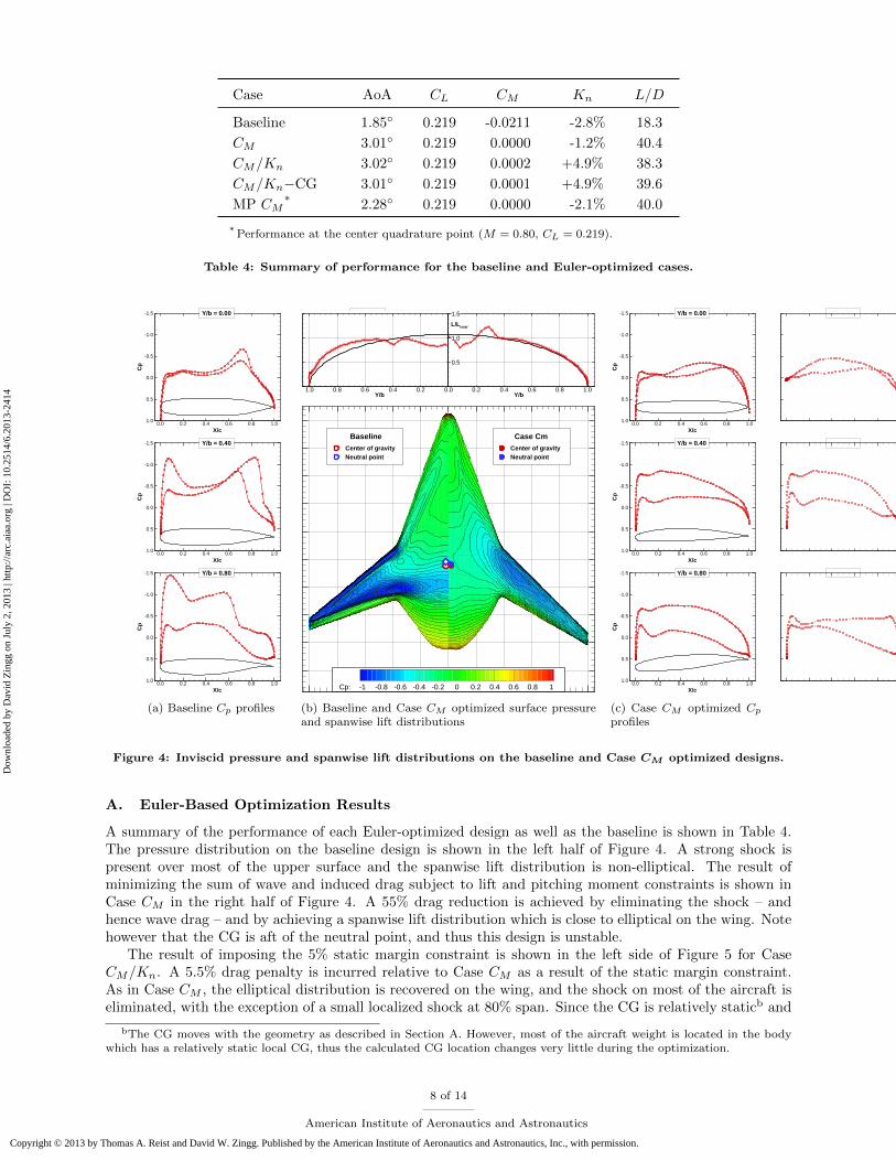
Case AoA CL CM Kn L/D

Baseline 1.85◦ 0.219 -0.0211 -2.8% 18.3

CM 3.01◦ 0.219 0.0000 -1.2% 40.4

CM/Kn 3.02◦ 0.219 0.0002 +4.9% 38.3

CM/Kn−CG 3.01◦ 0.219 0.0001 +4.9% 39.6

MP CM* 2.28◦ 0.219 0.0000 -2.1% 40.0

* Performance at the center quadrature point (M = 0.80, CL = 0.219).

Table 4: Summary of performance for the baseline and Euler-optimized cases.

X/c

Cp

0.0 0.2 0.4 0.6 0.8 1.0

-1.5

-1.0

-0.5

0.0

0.5

1.0

Y/b = 0.20

X/c

Cp

0.0 0.2 0.4 0.6 0.8 1.0

-1.5

-1.0

-0.5

0.0

0.5

1.0

Y/b = 0.40

X/c

Cp

0.0 0.2 0.4 0.6 0.8 1.0

-1.5

-1.0

-0.5

0.0

0.5

1.0

Y/b = 0.80

X/c

Cp

0.0 0.2 0.4 0.6 0.8 1.0

-1.5

-1.0

-0.5

0.0

0.5

1.0

Y/b = 0.00

X/c

Cp

0.0 0.2 0.4 0.6 0.8 1.0

-1.5

-1.0

-0.5

0.0

0.5

1.0

Y/b = 0.60

X/c

Cp

0.0 0.2 0.4 0.6 0.8 1.0

-1.5

-1.0

-0.5

0.0

0.5

1.0

Y/b = 0.98

(a) Baseline Cp profiles

Y/b0.00.20.40.60.81.0

Y/b0.0 0.2 0.4 0.6 0.8 1.0

0.5

1.0

1.5

L/Ltotal

Cp: -1 -0.8 -0.6 -0.4 -0.2 0 0.2 0.4 0.6 0.8 1

Center of gravityNeutral point

Case CmCenter of gravityNeutral point

Baseline

(b) Baseline and Case CM optimized surface pressureand spanwise lift distributions

X/c

Cp

0.0 0.2 0.4 0.6 0.8 1.0

-1.5

-1.0

-0.5

0.0

0.5

1.0

Y/b = 0.20

X/c

Cp

0.0 0.2 0.4 0.6 0.8 1.0

-1.5

-1.0

-0.5

0.0

0.5

1.0

Y/b = 0.40

X/c

Cp

0.0 0.2 0.4 0.6 0.8 1.0

-1.5

-1.0

-0.5

0.0

0.5

1.0

Y/b = 0.80

X/c

Cp

0.0 0.2 0.4 0.6 0.8 1.0

-1.5

-1.0

-0.5

0.0

0.5

1.0

Y/b = 0.00

X/c

Cp

0.0 0.2 0.4 0.6 0.8 1.0

-1.5

-1.0

-0.5

0.0

0.5

1.0

Y/b = 0.60

X/c

Cp

0.0 0.2 0.4 0.6 0.8 1.0

-1.5

-1.0

-0.5

0.0

0.5

1.0

Y/b = 0.98

(c) Case CM optimized Cp

profiles

Figure 4: Inviscid pressure and spanwise lift distributions on the baseline and Case CM optimized designs.

A. Euler-Based Optimization Results

A summary of the performance of each Euler-optimized design as well as the baseline is shown in Table 4.The pressure distribution on the baseline design is shown in the left half of Figure 4. A strong shock ispresent over most of the upper surface and the spanwise lift distribution is non-elliptical. The result ofminimizing the sum of wave and induced drag subject to lift and pitching moment constraints is shown inCase CM in the right half of Figure 4. A 55% drag reduction is achieved by eliminating the shock – andhence wave drag – and by achieving a spanwise lift distribution which is close to elliptical on the wing. Notehowever that the CG is aft of the neutral point, and thus this design is unstable.

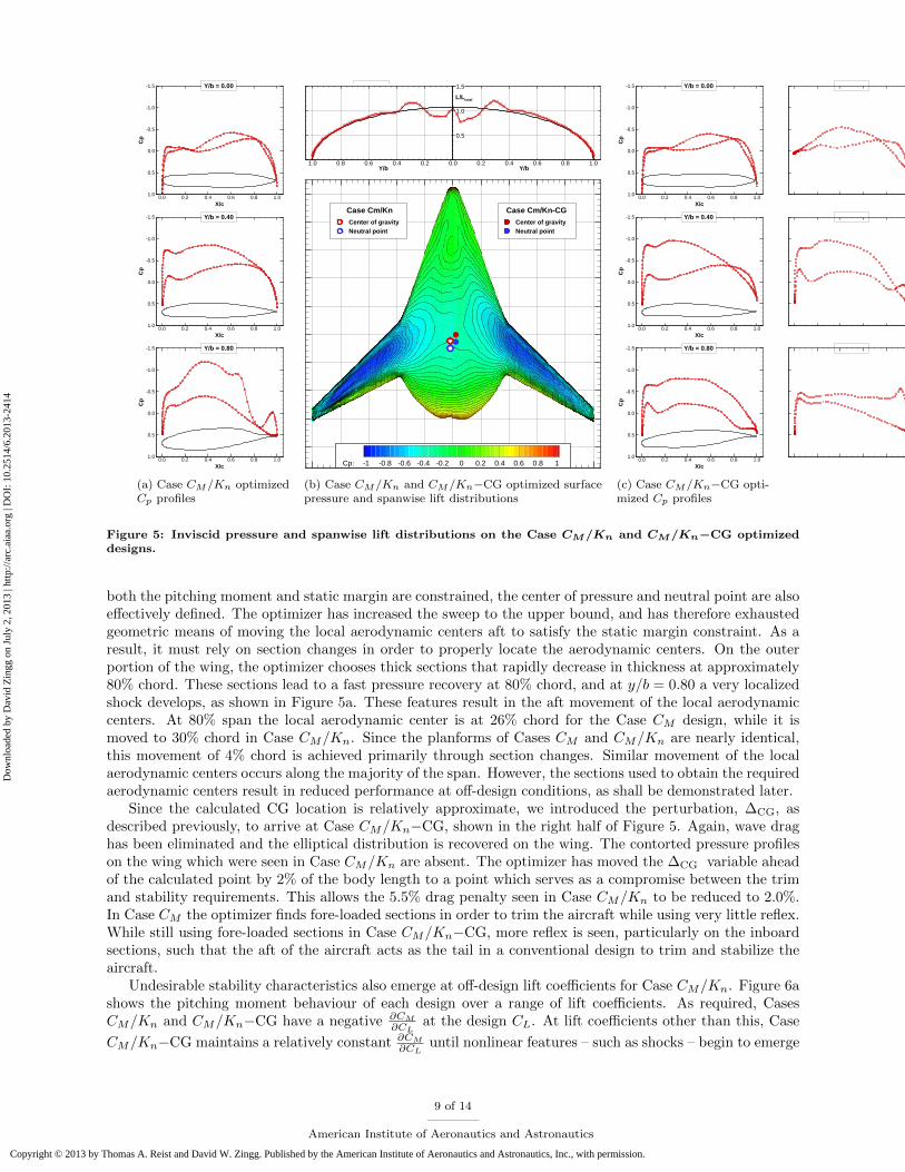
The result of imposing the 5% static margin constraint is shown in the left side of Figure 5 for CaseCM/Kn. A 5.5% drag penalty is incurred relative to Case CM as a result of the static margin constraint.As in Case CM , the elliptical distribution is recovered on the wing, and the shock on most of the aircraft iseliminated, with the exception of a small localized shock at 80% span. Since the CG is relatively staticb and

bThe CG moves with the geometry as described in Section A. However, most of the aircraft weight is located in the bodywhich has a relatively static local CG, thus the calculated CG location changes very little during the optimization.

8 of 14


Dow

nloa

ded

by D

avid

Zin

gg o

n Ju

ly 2

, 201

3 | h

ttp://

arc.

aiaa

.org

| D

OI:

10.

2514

/6.2

013-

2414


X/c

Cp

0.0 0.2 0.4 0.6 0.8 1.0

-1.5

-1.0

-0.5

0.0

0.5

1.0

Y/b = 0.20

X/c

Cp

0.0 0.2 0.4 0.6 0.8 1.0

-1.5

-1.0

-0.5

0.0

0.5

1.0

Y/b = 0.40

X/c

Cp

0.0 0.2 0.4 0.6 0.8 1.0

-1.5

-1.0

-0.5

0.0

0.5

1.0

Y/b = 0.80

X/c

Cp

0.0 0.2 0.4 0.6 0.8 1.0

-1.5

-1.0

-0.5

0.0

0.5

1.0

Y/b = 0.00

X/c

Cp

0.0 0.2 0.4 0.6 0.8 1.0

-1.5

-1.0

-0.5

0.0

0.5

1.0

Y/b = 0.60

X/c

Cp

0.0 0.2 0.4 0.6 0.8 1.0

-1.5

-1.0

-0.5

0.0

0.5

1.0

Y/b = 0.98

(a) Case CM/Kn optimizedCp profiles

Y/b0.00.20.40.60.81.0

Y/b0.0 0.2 0.4 0.6 0.8 1.0

0.5

1.0

1.5

L/L total

Cp: -1 -0.8 -0.6 -0.4 -0.2 0 0.2 0.4 0.6 0.8 1


Case Cm/Kn-CGCenter of gravityNeutral point

Case Cm/Kn

(b) Case CM/Kn and CM/Kn−CG optimized surfacepressure and spanwise lift distributions

X/c

Cp

0.0 0.2 0.4 0.6 0.8 1.0

-1.5

-1.0

-0.5

0.0

0.5

1.0

Y/b = 0.20

X/c

Cp

0.0 0.2 0.4 0.6 0.8 1.0

-1.5

-1.0

-0.5

0.0

0.5

1.0

Y/b = 0.40

X/c

Cp

0.0 0.2 0.4 0.6 0.8 1.0

-1.5

-1.0

-0.5

0.0

0.5

1.0

Y/b = 0.80

X/c

Cp

0.0 0.2 0.4 0.6 0.8 1.0

-1.5

-1.0

-0.5

0.0

0.5

1.0

Y/b = 0.00

X/c

Cp

0.0 0.2 0.4 0.6 0.8 1.0

-1.5

-1.0

-0.5

0.0

0.5

1.0

Y/b = 0.60

X/c

Cp

0.0 0.2 0.4 0.6 0.8 1.0

-1.5

-1.0

-0.5

0.0

0.5

1.0

Y/b = 0.98

(c) Case CM/Kn−CG opti-mized Cp profiles

Figure 5: Inviscid pressure and spanwise lift distributions on the Case CM/Kn and CM/Kn−CG optimizeddesigns.

both the pitching moment and static margin are constrained, the center of pressure and neutral point are alsoeffectively defined. The optimizer has increased the sweep to the upper bound, and has therefore exhaustedgeometric means of moving the local aerodynamic centers aft to satisfy the static margin constraint. As aresult, it must rely on section changes in order to properly locate the aerodynamic centers. On the outerportion of the wing, the optimizer chooses thick sections that rapidly decrease in thickness at approximately80% chord. These sections lead to a fast pressure recovery at 80% chord, and at y/b = 0.80 a very localizedshock develops, as shown in Figure 5a. These features result in the aft movement of the local aerodynamiccenters. At 80% span the local aerodynamic center is at 26% chord for the Case CM design, while it ismoved to 30% chord in Case CM/Kn. Since the planforms of Cases CM and CM/Kn are nearly identical,this movement of 4% chord is achieved primarily through section changes. Similar movement of the localaerodynamic centers occurs along the majority of the span. However, the sections used to obtain the requiredaerodynamic centers result in reduced performance at off-design conditions, as shall be demonstrated later.

Since the calculated CG location is relatively approximate, we introduced the perturbation, ∆CG, asdescribed previously, to arrive at Case CM/Kn−CG, shown in the right half of Figure 5. Again, wave draghas been eliminated and the elliptical distribution is recovered on the wing. The contorted pressure profileson the wing which were seen in Case CM/Kn are absent. The optimizer has moved the ∆CG variable aheadof the calculated point by 2% of the body length to a point which serves as a compromise between the trimand stability requirements. This allows the 5.5% drag penalty seen in Case CM/Kn to be reduced to 2.0%.In Case CM the optimizer finds fore-loaded sections in order to trim the aircraft while using very little reflex.While still using fore-loaded sections in Case CM/Kn−CG, more reflex is seen, particularly on the inboardsections, such that the aft of the aircraft acts as the tail in a conventional design to trim and stabilize theaircraft.

Undesirable stability characteristics also emerge at off-design lift coefficients for Case CM/Kn. Figure 6ashows the pitching moment behaviour of each design over a range of lift coefficients. As required, CasesCM/Kn and CM/Kn−CG have a negative ∂CM

∂CLat the design CL. At lift coefficients other than this, Case

CM/Kn−CG maintains a relatively constant ∂CM

∂CLuntil nonlinear features – such as shocks – begin to emerge

9 of 14


Dow

nloa

ded

by D

avid

Zin

gg o

n Ju

ly 2

, 201

3 | h

ttp://

arc.

aiaa

.org

| D

OI:

10.

2514

/6.2

013-

2414


Trim

CL

CL

CD

-0.2 -0.1 0.0 0.1 0.2 0.3 0.4 0.50.000

0.005

0.010

0.015

0.020

0.025

0.030 BaselineCmCm/KnCm-CGCm/Kn-CGCm MP

Trim C M

Trim

CL

CL

CM

-0.2 -0.1 0.0 0.1 0.2 0.3 0.4 0.5-0.030

-0.025

-0.020

-0.015

-0.010

-0.005

0.000

0.005

0.010

0.015

0.020

0.025

0.030 BaselineCmCm/KnCm/Kn-CGMP Cm

AoA

CL

-3 -2 -1 0 1 2 3 4 5 6 7-0.10

-0.05

0.00

0.05

0.10

0.15

0.20

0.25

0.30

0.35

0.40

0.45


Trim C M

AoA

CM

-3 -2 -1 0 1 2 3 4 5 6 7-0.030

-0.025

-0.020

-0.015

-0.010

-0.005

0.000

0.005

0.010

0.015

0.020

0.025


(a) Pitching moment behaviour over a range of lifts

Mach number

ML/

D

0.70 0.75 0.80 0.85 0.900

5

10

15

20

25

30

35

40BaselineCmCm/KnCm/Kn-CGMP Cm

Mach number

CD

0.70 0.75 0.80 0.85 0.900.000

0.005

0.010

0.015

0.020

0.025

0.030

0.035

0.040

0.045

0.050BaselineCmCm/KnCm-CGCm/Kn-CGCm MP

Mach number

CD M

2

0.70 0.75 0.80 0.85 0.900.000

0.005

0.010

0.015

0.020

0.025

0.030

0.035

0.040BaselineCmCm/KnCm-CGCm/Kn-CGCm MP

Mach number

Ran

ge F

acto

r

0.70 0.75 0.80 0.85 0.900

5

10

15

20

25

30

35

40

45BaselineCmCm/KnCm-CGCm/Kn-CGCm MP

(b) ML/D parameter over a range of cruise speeds

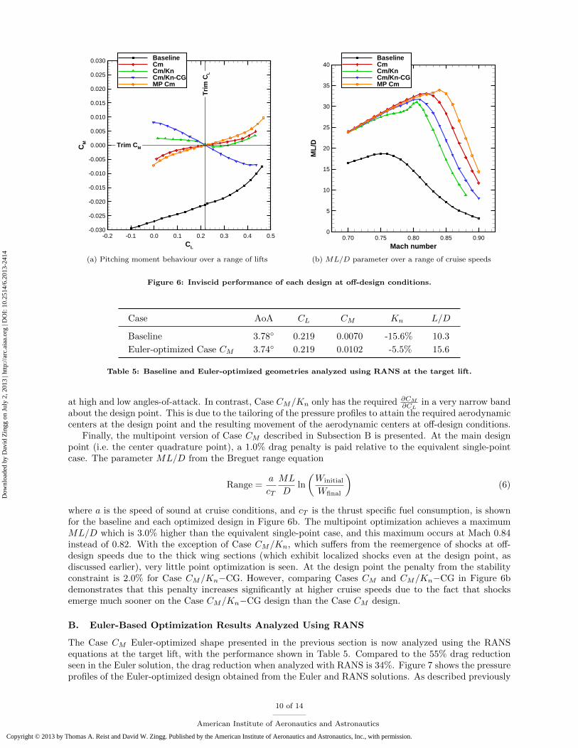
Figure 6: Inviscid performance of each design at off-design conditions.


Baseline 3.78◦ 0.219 0.0070 -15.6% 10.3

Euler-optimized Case CM 3.74◦ 0.219 0.0102 -5.5% 15.6

Table 5: Baseline and Euler-optimized geometries analyzed using RANS at the target lift.

at high and low angles-of-attack. In contrast, Case CM/Kn only has the required ∂CM

∂CLin a very narrow band

about the design point. This is due to the tailoring of the pressure profiles to attain the required aerodynamiccenters at the design point and the resulting movement of the aerodynamic centers at off-design conditions.

Finally, the multipoint version of Case CM described in Subsection B is presented. At the main designpoint (i.e. the center quadrature point), a 1.0% drag penalty is paid relative to the equivalent single-pointcase. The parameter ML/D from the Breguet range equation

Range =a

cT

ML

Dln

(Winitial

Wfinal

)(6)

where a is the speed of sound at cruise conditions, and cT is the thrust specific fuel consumption, is shownfor the baseline and each optimized design in Figure 6b. The multipoint optimization achieves a maximumML/D which is 3.0% higher than the equivalent single-point case, and this maximum occurs at Mach 0.84instead of 0.82. With the exception of Case CM/Kn, which suffers from the reemergence of shocks at off-design speeds due to the thick wing sections (which exhibit localized shocks even at the design point, asdiscussed earlier), very little point optimization is seen. At the design point the penalty from the stabilityconstraint is 2.0% for Case CM/Kn−CG. However, comparing Cases CM and CM/Kn−CG in Figure 6bdemonstrates that this penalty increases significantly at higher cruise speeds due to the fact that shocksemerge much sooner on the Case CM/Kn−CG design than the Case CM design.

B. Euler-Based Optimization Results Analyzed Using RANS

The Case CM Euler-optimized shape presented in the previous section is now analyzed using the RANSequations at the target lift, with the performance shown in Table 5. Compared to the 55% drag reductionseen in the Euler solution, the drag reduction when analyzed with RANS is 34%. Figure 7 shows the pressureprofiles of the Euler-optimized design obtained from the Euler and RANS solutions. As described previously

10 of 14


Dow

nloa

ded

by D

avid

Zin

gg o

n Ju

ly 2

, 201

3 | h

ttp://

arc.

aiaa

.org

| D

OI:

10.

2514

/6.2

013-

2414


X/c

Cp

0.0 0.2 0.4 0.6 0.8 1.0

-1.0

-0.5

0.0

0.5

1.0

Y/b = 0.20

X/c

Cp

0.0 0.2 0.4 0.6 0.8 1.0

-1.0

-0.5

0.0

0.5

1.0

Y/b = 0.40

X/c

Cp

0.0 0.2 0.4 0.6 0.8 1.0

-1.0

-0.5

0.0

0.5

1.0

Y/b = 0.80

X/c

Cp

0.0 0.2 0.4 0.6 0.8 1.0

-1.0

-0.5

0.0

0.5

1.0

Y/b = 0.60

X/c

Cp

0.0 0.2 0.4 0.6 0.8 1.0

-1.0

-0.5

0.0

0.5

1.0

Y/b = 0.98

X/c

Cp

0.0 0.2 0.4 0.6 0.8 1.0

-1.0

-0.5

0.0

0.5

1.0

Y/b = 0.00

Euler solution RANS solution

X/c

Cp

0.0 0.2 0.4 0.6 0.8 1.0

-1.0

-0.5

0.0

0.5

1.0

Y/b = 0.20

X/c

Cp

0.0 0.2 0.4 0.6 0.8 1.0

-1.0

-0.5

0.0

0.5

1.0

Y/b = 0.40

X/c

Cp

0.0 0.2 0.4 0.6 0.8 1.0

-1.0

-0.5

0.0

0.5

1.0

Y/b = 0.80

X/c

Cp

0.0 0.2 0.4 0.6 0.8 1.0

-1.0

-0.5

0.0

0.5

1.0

Y/b = 0.60

X/c

Cp

0.0 0.2 0.4 0.6 0.8 1.0

-1.0

-0.5

0.0

0.5

1.0

Y/b = 0.98

X/c

Cp

0.0 0.2 0.4 0.6 0.8 1.0

-1.0

-0.5

0.0

0.5

1.0

Y/b = 0.00


X/c

Cp

0.0 0.2 0.4 0.6 0.8 1.0

-1.0

-0.5

0.0

0.5

1.0

Y/b = 0.20

X/c

Cp

0.0 0.2 0.4 0.6 0.8 1.0

-1.0

-0.5

0.0

0.5

1.0

Y/b = 0.40

X/c

Cp

0.0 0.2 0.4 0.6 0.8 1.0

-1.0

-0.5

0.0

0.5

1.0

Y/b = 0.80

X/c

Cp

0.0 0.2 0.4 0.6 0.8 1.0

-1.0

-0.5

0.0

0.5

1.0

Y/b = 0.60

X/c

Cp

0.0 0.2 0.4 0.6 0.8 1.0

-1.0

-0.5

0.0

0.5

1.0

Y/b = 0.98

X/c

Cp

0.0 0.2 0.4 0.6 0.8 1.0

-1.0

-0.5

0.0

0.5

1.0

Y/b = 0.00

Euler solution RANS solutionX/c

Cp

0.0 0.2 0.4 0.6 0.8 1.0

-1.0

-0.5

0.0

0.5

1.0

Y/b = 0.20

X/c

Cp

0.0 0.2 0.4 0.6 0.8 1.0

-1.0

-0.5

0.0

0.5

1.0

Y/b = 0.40

X/c

Cp

0.0 0.2 0.4 0.6 0.8 1.0

-1.0

-0.5

0.0

0.5

1.0

Y/b = 0.80

X/c

Cp

0.0 0.2 0.4 0.6 0.8 1.0

-1.0

-0.5

0.0

0.5

1.0

Y/b = 0.60

X/c

Cp

0.0 0.2 0.4 0.6 0.8 1.0

-1.0

-0.5

0.0

0.5

1.0

Y/b = 0.98

X/c

Cp

0.0 0.2 0.4 0.6 0.8 1.0

-1.0

-0.5

0.0

0.5

1.0

Y/b = 0.00


X/c

Cp

0.0 0.2 0.4 0.6 0.8 1.0

-1.0

-0.5

0.0

0.5

1.0

Y/b = 0.20

X/c

Cp

0.0 0.2 0.4 0.6 0.8 1.0

-1.0

-0.5

0.0

0.5

1.0

Y/b = 0.40

X/c

Cp

0.0 0.2 0.4 0.6 0.8 1.0

-1.0

-0.5

0.0

0.5

1.0

Y/b = 0.80

X/c

Cp

0.0 0.2 0.4 0.6 0.8 1.0

-1.0

-0.5

0.0

0.5

1.0

Y/b = 0.60

X/c

Cp

0.0 0.2 0.4 0.6 0.8 1.0

-1.0

-0.5

0.0

0.5

1.0

Y/b = 0.98

X/c

Cp

0.0 0.2 0.4 0.6 0.8 1.0

-1.0

-0.5

0.0

0.5

1.0

Y/b = 0.00

Euler solution RANS solutionX/c

Cp

0.0 0.2 0.4 0.6 0.8 1.0

-1.0

-0.5

0.0

0.5

1.0

Y/b = 0.20

X/c

Cp

0.0 0.2 0.4 0.6 0.8 1.0

-1.0

-0.5

0.0

0.5

1.0

Y/b = 0.40

X/c

Cp

0.0 0.2 0.4 0.6 0.8 1.0

-1.0

-0.5

0.0

0.5

1.0

Y/b = 0.80

X/c

Cp

0.0 0.2 0.4 0.6 0.8 1.0

-1.0

-0.5

0.0

0.5

1.0

Y/b = 0.60

X/c

Cp

0.0 0.2 0.4 0.6 0.8 1.0

-1.0

-0.5

0.0

0.5

1.0

Y/b = 0.98

X/c

Cp

0.0 0.2 0.4 0.6 0.8 1.0

-1.0

-0.5

0.0

0.5

1.0

Y/b = 0.00


X/c

Cp

0.0 0.2 0.4 0.6 0.8 1.0

-1.0

-0.5

0.0

0.5

1.0

Y/b = 0.20

X/c

Cp

0.0 0.2 0.4 0.6 0.8 1.0

-1.0

-0.5

0.0

0.5

1.0

Y/b = 0.40

X/c

Cp

0.0 0.2 0.4 0.6 0.8 1.0

-1.0

-0.5

0.0

0.5

1.0

Y/b = 0.80

X/c

Cp

0.0 0.2 0.4 0.6 0.8 1.0

-1.0

-0.5

0.0

0.5

1.0

Y/b = 0.60

X/c

Cp

0.0 0.2 0.4 0.6 0.8 1.0

-1.0

-0.5

0.0

0.5

1.0

Y/b = 0.98

X/c

Cp

0.0 0.2 0.4 0.6 0.8 1.0

-1.0

-0.5

0.0

0.5

1.0

Y/b = 0.00


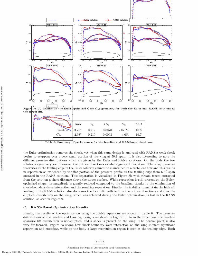
Figure 7: Cp profiles on the Euler-optimized Case CM geometry for both the Euler and RANS solutions atthe target lift.


Baseline 3.78◦ 0.219 0.0070 -15.6% 10.3

CM 2.98◦ 0.219 0.0003 -4.0% 16.7

Table 6: Summary of performance for the baseline and RANS-optimized case.

the Euler-optimization removes the shock, yet when this same design is analyzed with RANS a weak shockbegins to reappear over a very small portion of the wing at 50% span. It is also interesting to note thedifferent pressure distributions which are given by the Euler and RANS solutions. On the body the twosolutions agree very well; however the outboard sections exhibit significant deviation. The sharp pressurerecoveries at the trailing edge in the Euler solution cannot be maintained in a turbulent flow and this resultsin separation as evidenced by the flat portion of the pressure profile at the trailing edge from 60% spanoutward in the RANS solution. This separation is visualized in Figure 8b with stream traces extractedfrom the solution a short distance above the upper surface. While separation is still present on the Euler-optimized shape, its magnitude is greatly reduced compared to the baseline, thanks to the elimination ofshock-boundary-layer interaction and the resulting separation. Finally, the inability to maintain the high aftloading in the RANS solution also decreases the local lift coefficient on the outboard sections and thus theelliptical distribution on the wing, which was achieved during the Euler optimization, is lost in the RANSsolution, as seen in Figure 9.

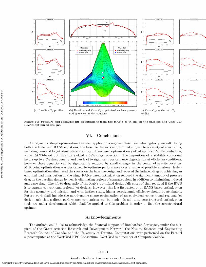
C. RANS-Based Optimization Results

Finally, the results of the optimization using the RANS equations are shown in Table 6. The pressuredistributions on the baseline and Case CM designs are shown in Figure 10. As in the Euler case, the baselinespanwise lift distribution is non-elliptical and a shock is present on the wing. The neutral point is alsovery far forward. Figure 8a shows how shock-boundary-layer interaction on the wing induces significantseparation and crossflow, while on the body a large recirculation region is seen at the trailing edge. Both

11 of 14


Dow

nloa

ded

by D

avid

Zin

gg o

n Ju

ly 2

, 201

3 | h

ttp://

arc.

aiaa

.org

| D

OI:

10.

2514

/6.2

013-

2414


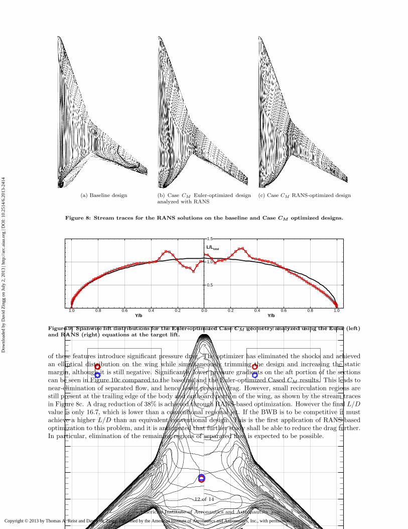
(a) Baseline design (b) Case CM Euler-optimized designanalyzed with RANS

(c) Case CM RANS-optimized design

Figure 8: Stream traces for the RANS solutions on the baseline and Case CM optimized designs.

Y/b0.00.20.40.60.81.0

Y/b0.0 0.2 0.4 0.6 0.8 1.0

0.5

1.0

1.5

L/Ltotal

Cp: -1 -0.8 -0.6 -0.4 -0.2 0 0.2 0.4 0.6 0.8 1


RANS analyzedCenter of gravityNeutral point

Euler analyzed

Figure 9: Spanwise lift distributions for the Euler-optimized Case CM geometry analyzed using the Euler (left)and RANS (right) equations at the target lift.

of these features introduce significant pressure drag. The optimizer has eliminated the shocks and achievedan elliptical distribution on the wing while simultaneously trimming the design and increasing the staticmargin, although it is still negative. Significantly lower pressure gradients on the aft portion of the sectionscan be seen in Figure 10c compared to the baseline and the Euler-optimized Cased CM results. This leads tonear-elimination of separated flow, and hence lower pressure drag. However, small recirculation regions arestill present at the trailing edge of the body and outboard portion of the wing, as shown by the stream tracesin Figure 8c. A drag reduction of 38% is achieved through RANS-based optimization. However the final L/Dvalue is only 16.7, which is lower than a conventional regional jet. If the BWB is to be competitive it mustachieve a higher L/D than an equivalent conventional design. This is the first application of RANS-basedoptimization to this problem, and it is anticipated that further study shall be able to reduce the drag further.In particular, elimination of the remaining regions of separated flow is expected to be possible.

12 of 14


Dow

nloa

ded

by D

avid

Zin

gg o

n Ju

ly 2

, 201

3 | h

ttp://

arc.

aiaa

.org

| D

OI:

10.

2514

/6.2

013-

2414


X/c

Cp

0.0 0.2 0.4 0.6 0.8 1.0

-2.0

-1.5

-1.0

-0.5

0.0

0.5

1.0

Y/b = 0.20

X/c

Cp

0.0 0.2 0.4 0.6 0.8 1.0

-2.0

-1.5

-1.0

-0.5

0.0

0.5

1.0

Y/b = 0.40

X/c

Cp

0.0 0.2 0.4 0.6 0.8 1.0

-2.0

-1.5

-1.0

-0.5

0.0

0.5

1.0

Y/b = 0.80

X/c

Cp

0.0 0.2 0.4 0.6 0.8 1.0

-2.0

-1.5

-1.0

-0.5

0.0

0.5

1.0

Y/b = 0.00

X/c

Cp

0.0 0.2 0.4 0.6 0.8 1.0

-2.0

-1.5

-1.0

-0.5

0.0

0.5

1.0

Y/b = 0.60

X/c

Cp

0.0 0.2 0.4 0.6 0.8 1.0

-2.0

-1.5

-1.0

-0.5

0.0

0.5

1.0

Y/b = 0.98

(a) Baseline Cp profiles

Y/b0.00.20.40.60.81.0

Y/b0.0 0.2 0.4 0.6 0.8 1.0

0.5

1.0

1.5

L/Ltotal

Cp: -1 -0.8 -0.6 -0.4 -0.2 0 0.2 0.4 0.6 0.8 1


Case CmCenter of gravityNeutral point

Baseline

(b) Baseline and Case CM optimized surface pressureand spanwise lift distributions

X/c

Cp

0.0 0.2 0.4 0.6 0.8 1.0

-2.0

-1.5

-1.0

-0.5

0.0

0.5

1.0

Y/b = 0.20

X/c

Cp

0.0 0.2 0.4 0.6 0.8 1.0

-2.0

-1.5

-1.0

-0.5

0.0

0.5

1.0

Y/b = 0.40

X/c

Cp

0.0 0.2 0.4 0.6 0.8 1.0

-2.0

-1.5

-1.0

-0.5

0.0

0.5

1.0

Y/b = 0.80

X/c

Cp

0.0 0.2 0.4 0.6 0.8 1.0

-2.0

-1.5

-1.0

-0.5

0.0

0.5

1.0

Y/b = 0.00

X/c

Cp

0.0 0.2 0.4 0.6 0.8 1.0

-2.0

-1.5

-1.0

-0.5

0.0

0.5

1.0

Y/b = 0.60

X/c

Cp

0.0 0.2 0.4 0.6 0.8 1.0

-2.0

-1.5

-1.0

-0.5

0.0

0.5

1.0

Y/b = 0.98

(c) Case CM optimized Cp

profiles

Figure 10: Pressure and spanwise lift distributions from the RANS solutions on the baseline and Case CM

RANS-optimized designs.

VI. Conclusions

Aerodynamic shape optimization has been applied to a regional class blended-wing-body aircraft. Usingboth the Euler and RANS equations, the baseline design was optimized subject to a variety of constraints;including trim and longitudinal static stability. Euler-based optimization yielded up to a 55% drag reduction,while RANS-based optimization yielded a 38% drag reduction. The imposition of a stability constraintincurs up to a 5% drag penalty and can lead to significant performance degradation at off-design conditions;however these penalties can be significantly reduced by small changes in the center of gravity location.Multipoint optimization was performed to optimize performance over a range of possible missions. Euler-based optimization eliminated the shocks on the baseline design and reduced the induced drag by achieving anelliptical load distribution on the wing. RANS-based optimization reduced the significant amount of pressuredrag on the baseline design by nearly eliminating regions of separated flow, in addition to minimizing inducedand wave drag. The lift-to-drag ratio of the RANS-optimized design falls short of that required if the BWBis to surpass conventional regional jet designs. However, this is a first attempt at RANS-based optimizationfor this geometry and mission, and with further study, higher aerodynamic efficiency should be attainable.Future work shall include the aerodynamic shape optimization of an equivalent conventional regional jetdesign such that a direct performance comparison can be made. In addition, aerostructural optimizationtools are under development which shall be applied to this problem in order to find the aerostructuraloptimum.

Acknowledgments

The authors would like to acknowledge the financial support of Bombardier Aerospace, under the aus-pices of the Green Aviation Research and Development Network, the Natural Sciences and EngineeringResearch Council of Canada, and the University of Toronto. Computations were performed on the Parallelsupercomputer at the WestGrid HPC Consortium. WestGrid is a member of Compute Canada.

13 of 14


Dow

nloa

ded

by D

avid

Zin

gg o

n Ju

ly 2

, 201

3 | h

ttp://

arc.

aiaa

.org

| D

OI:

10.

2514

/6.2

013-

2414


References

1Liebeck, R., “Design of the Blended Wing Body Subsonic Transport,” Journal of Aircraft , Vol. 41, No. 1, 2004, pp. 10–25.2Hileman, J. I., Spakovszky, Z. S., Drela, M., Sargeant, M. A., and Jones, A., “Airframe Design for Silent Fuel-Efficient

Aircraft,” Journal of Aircraft , Vol. 47, No. 3, 2010, pp. 956–969.3Li, V. and Velicki, A., “Advanced PRSEUS Structural Concept Design and Optimization,” 12th AIAA/ISSMO Multi-

disciplinary Analysis and Optimization Conference, AIAA-2008-5840, Victoria, BC, September 2008.4Mukhopadhyay, V., “Blended-Wing-Body Fuselage Structural Design for Weight Reduction,” 46th Structures, Structural

Dynamics and Materials Conference, AIAA-2005-2349, Austin, TX, April 2005.5Hansen, L. U., Heinze, W., and Horst, P., “Blended Wing Body Structures in Multidisciplinary Pre-Design,” Structural

and Multidisciplinary Optimization, Vol. 38, No. 1, 2008, pp. 93–106.6Vicroy, D. D., “Blended-Wing-Body Low-Speed Flight Dynamics: Summary of Ground Tests and Sample Results,” 47th

AIAA Aerospace Sciences Meeting and Exhibit , AIAA-2009-0933, Orlando, FL, January 2009.7Voskuijl, M., La Rocca, G., and Dircken, F., “Controllability of Blended Wing Body Aircraft,” 26th International

Congress of the Aeronautical Sciences, Anchorage, AL, September 2008.8Gern, F. H., “Improved Aerodynamic Analysis for Hybrid Wing Body Conceptual Design Optimization,” 50th AIAA

Aerospace Sciences Meeting and Exhibit , AIAA-2012-0249, Nashville, TN, January 2012.9Nickol, C. L., “Hybrid Wing Body Configuration Scaling Study,” 50th AIAA Aerospace Sciences Meeting and Exhibit ,

AIAA-2012-0337, Nashville, TN, January 2012.10Wakayama, S., “Blended-Wing-Body Optimization Problem Setup,” 8th AIAA/USAF/NASA/ISSMO Symposium on

Multidisciplinary Analysis and Optimization, AIAA-2000-4740, Long Beach, CA, September 2000.11Hileman, J. I., Spakovszky, Z. S., Drela, M., and Sargeant, M. A., “Airframe Design for “Silent Aircraft”,” 45th AIAA

Aerospace Sciences Meeting and Exhibit , AIAA-2007-0453, Reno, NV, January 2007.12Morris, A. J., “MOB: A European Distributed Multi-Disciplinary Design and Optimisation Project,” 9th AIAA/ISSMO

Symposium on Multidisciplinary Analysis and Optimization, AIAA-2002-5444, Atlanta, GA, September 2002.13Meheut, M., Grenon, R., Carrier, G., Defos, M., and Duffau, M., “Aerodynamic Design of Transonic Flying Wing

Configurations,” CEAS Katnet II Conference on Key Aerodynamic Technologies, Breme, Germany, May 2009.14Peigin, S. and Epstein, B., “Computational Fluid Dynamics Driven Optimization of Blended Wing Body Aircraft,” AIAA

Journal , Vol. 44, No. 11, 2006, pp. 2736–2745.15Qin, N., Vavalle, A., Le Moigne, A., Laban, M., Hackett, K., and Weinerfelt, P., “Aerodynamic Considerations of Blended

Wing Body Aircraft,” Progress in Aerospace Sciences, Vol. 40, No. 6, 2004, pp. 321–343.16Le Moigne, A. and Qin, N., “Aerofoil Profile and Sweep Optimisation for a Blended Wing-Body Aircraft Using A Discrete

Adjoint Method,” The Aeronautical Journal , Vol. 110, No. 1111, 2006, pp. 589–604.17Kuntawala, N. B., Hicken, J. E., and Zingg, D. W., “Preliminary Aerodynamic Shape Optimization Of A Blended-Wing-

Body Aircraft Configuration,” 49th AIAA Aerospace Sciences Meeting, AIAA-2011-0642, Orlando, FL, January 2011.18Hicken, J. E. and Zingg, D. W., “A Parallel Newton-Krylov Solver for the Euler Equations Discretized Using Simultaneous

Approximation Terms,” AIAA Journal , Vol. 46, No. 11, 2008, pp. 2773–2786.19Osusky, M. and Zingg, D. W., “A Parallel Newton-Krylov-Schur Flow Solver for the Reynolds-Averaged Navier-Stokes

Equations,” 50th AIAA Aerospace Sciences Meeting and Exhibit , AIAA-2012-0442, Nashville, TN, January 2012.20Hicken, J. E. and Zingg, D. W., “Aerodynamic Optimization Algorithm with Integrated Geometry Parameterization and

Mesh Movement,” AIAA Journal , Vol. 48, No. 2, 2010, pp. 401–413.21Zingg, D. W., Nemec, M., and Pulliam, T. H., “A Comparative Evaluation of Genetic and Gradient-Based Algorithms

Applied to Aerodynamic Optimization,” REMN , Vol. 17, No. 1, 2008, pp. 103–126.22Chernukhin, O. and Zingg, D. W., “Multimodality and Global Optimization in Aerodynamic Design,” AIAA Journal ,

Vol. 51, No. 6, 2013, pp. 1342–1354.23Gill, P. E., Murray, W., and Saunders, M. A., “SNOPT: An SQP Algorithm for Large-Scale Constrained Optimization,”

Society for Industrial Applied Mathematics Review , Vol. 47, No. 1, 2005, pp. 99–131.24Hicken, J. E. and Zingg, D. W., “Induced Drag Minimization of Nonplanar Geometries Based on the Euler Equations,”

AIAA Journal , Vol. 48, No. 11, 2010, pp. 2564–2575.25Osusky, L. and Zingg, D. W., “A Novel Aerodynamic Shape Optimization Approach for Three-Dimensional Turbulent

Flows,” 50th AIAA Aerospace Sciences Meeting and Exhibit , AIAA-2012-0058, Nashville, TN, January 2012.26Bradley, K. R., “A Sizing Methodology for the Conceptual Design of Blended-Wing-Body Transports,” Tech. Rep.

NASA/CR-2004-213016, NASA/Langley Research Center: Joint Institute for Advancement of Flight Sciences, 2004.27Roskam, J., Airplane Design Part V: Component Weight Estimation, Aviation and Engineering Corporation, 1989.28Mozdzanowska, A. and Hansman, R. J., “Evaluation of Regional Jet Operating Patterns in the Continental United

States,” Tech. Rep. ICAT-2004-1, International Center for Air Transportation, 2004.29Martınez-Val, R., Perez, E., Alfaro, P., and Perez, J., “Conceptual Design of a Medium Size Flying Wing,” Journal of

Aerospace Engineering, Vol. 221, No. 1, 2007, pp. 57–66.30Buckley, H. P. and Zingg, D. W., “An Approach to Aerodynamic Design Through Numerical Optimization,” AIAA

Journal , in press, 2013.

14 of 14


Dow

nloa

ded

by D

avid

Zin

gg o

n Ju

ly 2

, 201

3 | h

ttp://

arc.

aiaa

.org

| D

OI:

10.

2514

/6.2

013-

2414


Documents

Aerodynamic Shape Optimization of a Blended-Wing …oddjob.utias.utoronto.ca/dwz/Miscellaneous/Reist2013-2414.pdfBlended-Wing-Body Regional Transport ... system on the top of the aircraft